LYAPUNOV-BASED ROBUST AND ADAPTIVE CONTROL OF NONLINEARSYSTEMS USING A NOVEL FEEDBACK STRUCTURE

By

PARAG PATRE

A DISSERTATION PRESENTED TO THE GRADUATE SCHOOLOF THE UNIVERSITY OF FLORIDA IN PARTIAL FULFILLMENT

OF THE REQUIREMENTS FOR THE DEGREE OFDOCTOR OF PHILOSOPHY

UNIVERSITY OF FLORIDA

2009

1

c© 2009 Parag Patre

2

To my parents, Madhukar and Surekha Patre, and my sister, Aparna

3

ACKNOWLEDGMENTS

I would like to express sincere gratitude to my advisor, Dr. Warren E. Dixon, whose

experience and motivation were instrumental in successful completion of my PhD. I

appreciate his patience towards me and allowing me the freedom to work independently.

I would also like to extend my gratitude to my committee members Dr. Norman

Fitz-Coy, Dr. Rick Lind, Dr. Pramod Khargonekar, and Dr. Frank Lewis for the time and

help they provided.

I would like to thank my coworkers, family, and friends for their support and

encouragement.

4

TABLE OF CONTENTS

page

ACKNOWLEDGMENTS . . . . . . . . . . . . . . . . . . . . . . . . . . . . . . . . . 4

LIST OF TABLES . . . . . . . . . . . . . . . . . . . . . . . . . . . . . . . . . . . . . 8

LIST OF FIGURES . . . . . . . . . . . . . . . . . . . . . . . . . . . . . . . . . . . . 9

ABSTRACT . . . . . . . . . . . . . . . . . . . . . . . . . . . . . . . . . . . . . . . . 11

CHAPTER

1 INTRODUCTION . . . . . . . . . . . . . . . . . . . . . . . . . . . . . . . . . . 13

1.1 Motivation and Problem Statement . . . . . . . . . . . . . . . . . . . . . . 131.2 Contributions . . . . . . . . . . . . . . . . . . . . . . . . . . . . . . . . . . 18

2 ASYMPTOTIC TRACKING FOR SYSTEMS WITH STRUCTURED ANDUNSTRUCTURED UNCERTAINTIES . . . . . . . . . . . . . . . . . . . . . . . 22

2.1 Introduction . . . . . . . . . . . . . . . . . . . . . . . . . . . . . . . . . . . 222.2 Dynamic Model . . . . . . . . . . . . . . . . . . . . . . . . . . . . . . . . . 222.3 Error System Development . . . . . . . . . . . . . . . . . . . . . . . . . . . 242.4 Stability Analysis . . . . . . . . . . . . . . . . . . . . . . . . . . . . . . . . 282.5 Experimental Results . . . . . . . . . . . . . . . . . . . . . . . . . . . . . . 322.6 Discussion . . . . . . . . . . . . . . . . . . . . . . . . . . . . . . . . . . . . 392.7 Conclusions . . . . . . . . . . . . . . . . . . . . . . . . . . . . . . . . . . . 40

3 ASYMPTOTIC TRACKING FOR UNCERTAIN DYNAMIC SYSTEMS VIAA MULTILAYER NEURAL NETWORK FEEDFORWARD AND RISE FEEDBACKCONTROL STRUCTURE . . . . . . . . . . . . . . . . . . . . . . . . . . . . . . 43

3.1 Introduction . . . . . . . . . . . . . . . . . . . . . . . . . . . . . . . . . . . 433.2 Dynamic Model . . . . . . . . . . . . . . . . . . . . . . . . . . . . . . . . . 463.3 Control Objective . . . . . . . . . . . . . . . . . . . . . . . . . . . . . . . . 463.4 Feedforward NN Estimation . . . . . . . . . . . . . . . . . . . . . . . . . . 463.5 RISE Feedback Control Development . . . . . . . . . . . . . . . . . . . . . 49

3.5.1 Open-Loop Error System . . . . . . . . . . . . . . . . . . . . . . . . 493.5.2 Closed-Loop Error System . . . . . . . . . . . . . . . . . . . . . . . 50

3.6 Stability Analysis . . . . . . . . . . . . . . . . . . . . . . . . . . . . . . . . 543.7 Experiment . . . . . . . . . . . . . . . . . . . . . . . . . . . . . . . . . . . 58

3.7.1 Discussion . . . . . . . . . . . . . . . . . . . . . . . . . . . . . . . . 593.8 Conclusions . . . . . . . . . . . . . . . . . . . . . . . . . . . . . . . . . . . 61

4 A NEW CLASS OF MODULAR ADAPTIVE CONTROLLERS . . . . . . . . . 63

4.1 Introduction . . . . . . . . . . . . . . . . . . . . . . . . . . . . . . . . . . . 634.2 Dynamic System . . . . . . . . . . . . . . . . . . . . . . . . . . . . . . . . 65

5

4.3 Control Objective . . . . . . . . . . . . . . . . . . . . . . . . . . . . . . . . 664.4 Control Development . . . . . . . . . . . . . . . . . . . . . . . . . . . . . . 674.5 Modular Adaptive Update Law Development . . . . . . . . . . . . . . . . . 694.6 Stability Analysis . . . . . . . . . . . . . . . . . . . . . . . . . . . . . . . . 734.7 Neural Network Extension to Non-LP Systems . . . . . . . . . . . . . . . . 77

4.7.1 RISE Feedback Control Development . . . . . . . . . . . . . . . . . 774.7.2 Modular Tuning Law Development . . . . . . . . . . . . . . . . . . 79

4.8 Stability Analysis . . . . . . . . . . . . . . . . . . . . . . . . . . . . . . . . 824.9 Application to Euler-Lagrange Systems . . . . . . . . . . . . . . . . . . . . 824.10 Experiment . . . . . . . . . . . . . . . . . . . . . . . . . . . . . . . . . . . 83

4.10.1 Modular Adaptive Update Law . . . . . . . . . . . . . . . . . . . . 854.10.2 Modular Neural Network Update Law . . . . . . . . . . . . . . . . . 864.10.3 Discussion . . . . . . . . . . . . . . . . . . . . . . . . . . . . . . . . 92

4.11 Conclusion . . . . . . . . . . . . . . . . . . . . . . . . . . . . . . . . . . . . 94

5 COMPOSITE ADAPTIVE CONTROL FOR SYSTEMS WITH ADDITIVEDISTURBANCES . . . . . . . . . . . . . . . . . . . . . . . . . . . . . . . . . . 95

5.1 Introduction . . . . . . . . . . . . . . . . . . . . . . . . . . . . . . . . . . . 955.2 Dynamic System . . . . . . . . . . . . . . . . . . . . . . . . . . . . . . . . 965.3 Control Objective . . . . . . . . . . . . . . . . . . . . . . . . . . . . . . . . 975.4 Control Development . . . . . . . . . . . . . . . . . . . . . . . . . . . . . . 98

5.4.1 RISE-based Swapping . . . . . . . . . . . . . . . . . . . . . . . . . . 1005.4.2 Composite Adaptation . . . . . . . . . . . . . . . . . . . . . . . . . 1035.4.3 Closed-Loop Prediction Error System . . . . . . . . . . . . . . . . . 1035.4.4 Closed-Loop Tracking Error System . . . . . . . . . . . . . . . . . . 105

5.5 Stability Analysis . . . . . . . . . . . . . . . . . . . . . . . . . . . . . . . 1085.6 Experiment . . . . . . . . . . . . . . . . . . . . . . . . . . . . . . . . . . . 113

5.6.1 Discussion . . . . . . . . . . . . . . . . . . . . . . . . . . . . . . . . 1175.7 Conclusion . . . . . . . . . . . . . . . . . . . . . . . . . . . . . . . . . . . . 118

6 COMPOSITE ADAPTATION FOR NN-BASED CONTROLLERS . . . . . . . 119

6.1 Introduction . . . . . . . . . . . . . . . . . . . . . . . . . . . . . . . . . . . 1196.2 Dynamic System . . . . . . . . . . . . . . . . . . . . . . . . . . . . . . . . 1206.3 Control Objective . . . . . . . . . . . . . . . . . . . . . . . . . . . . . . . . 1216.4 Control Development . . . . . . . . . . . . . . . . . . . . . . . . . . . . . . 122

6.4.1 Swapping . . . . . . . . . . . . . . . . . . . . . . . . . . . . . . . . . 1246.4.2 Composite Adaptation . . . . . . . . . . . . . . . . . . . . . . . . . 1306.4.3 Closed-Loop Error System . . . . . . . . . . . . . . . . . . . . . . . 131

6.5 Stability Analysis . . . . . . . . . . . . . . . . . . . . . . . . . . . . . . . . 1356.6 Experiment . . . . . . . . . . . . . . . . . . . . . . . . . . . . . . . . . . . 139

6.6.1 Discussion . . . . . . . . . . . . . . . . . . . . . . . . . . . . . . . . 1406.7 Conclusion . . . . . . . . . . . . . . . . . . . . . . . . . . . . . . . . . . . . 142

6

7 CONCLUSIONS AND FUTURE WORK . . . . . . . . . . . . . . . . . . . . . . 144

7.1 Conclusions . . . . . . . . . . . . . . . . . . . . . . . . . . . . . . . . . . . 1447.2 Future Work . . . . . . . . . . . . . . . . . . . . . . . . . . . . . . . . . . . 146

APPENDIX . . . . . . . . . . . . . . . . . . . . . . . . . . . . . . . . . . . . . . . . . 147

REFERENCES . . . . . . . . . . . . . . . . . . . . . . . . . . . . . . . . . . . . . . . 157

BIOGRAPHICAL SKETCH . . . . . . . . . . . . . . . . . . . . . . . . . . . . . . . . 163

7

LIST OF TABLES

Table page

2-1 t-test: two samples assuming equal variances for RMS error . . . . . . . . . . . 41

2-2 t-test: two samples assuming equal variances for RMS torque . . . . . . . . . . . 42

4-1 LP case: Average RMS values for 10 trials . . . . . . . . . . . . . . . . . . . . . 86

4-2 Non-LP case: Average RMS values for 10 trials . . . . . . . . . . . . . . . . . . 90

8

LIST OF FIGURES

Figure page

2-1 The experimental testbed consists of a circular disk mounted on a NSK direct-driveswitched reluctance motor. . . . . . . . . . . . . . . . . . . . . . . . . . . . . . . 33

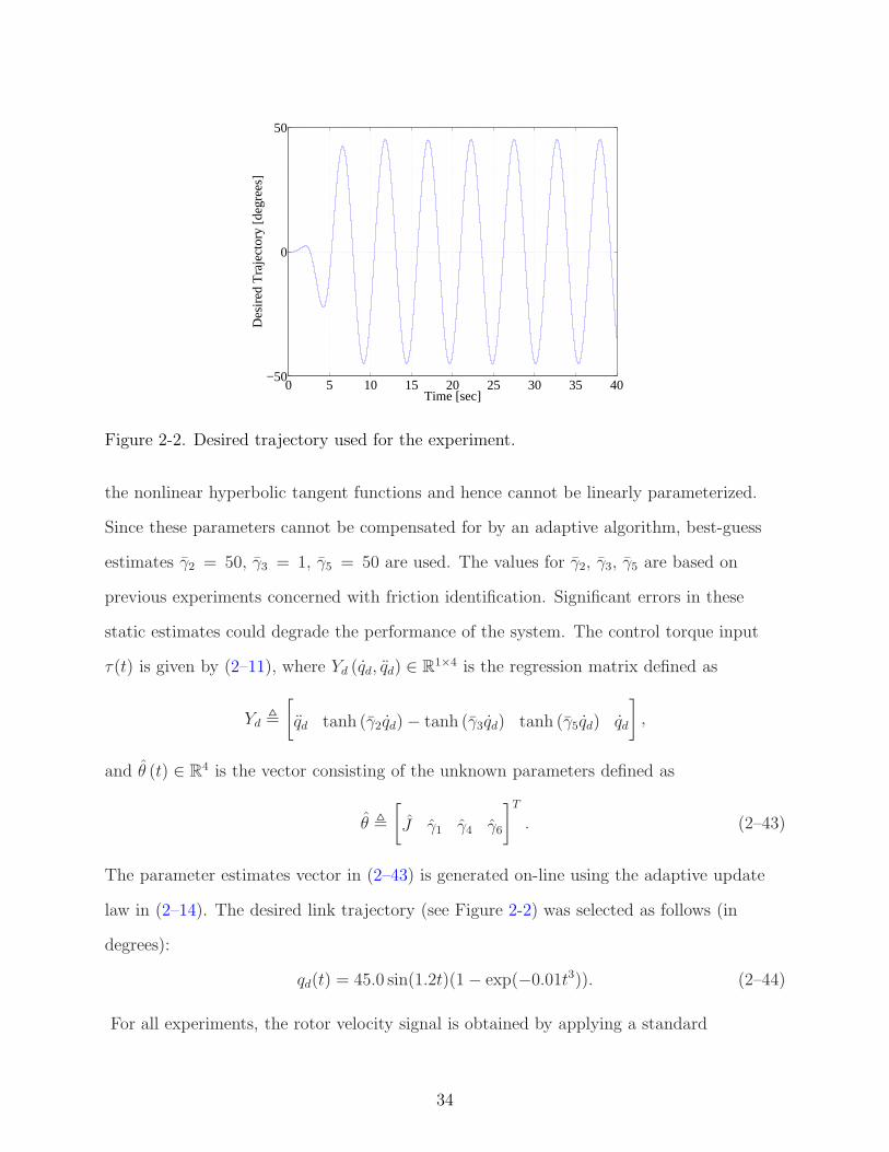
2-2 Desired trajectory used for the experiment. . . . . . . . . . . . . . . . . . . . . . 34

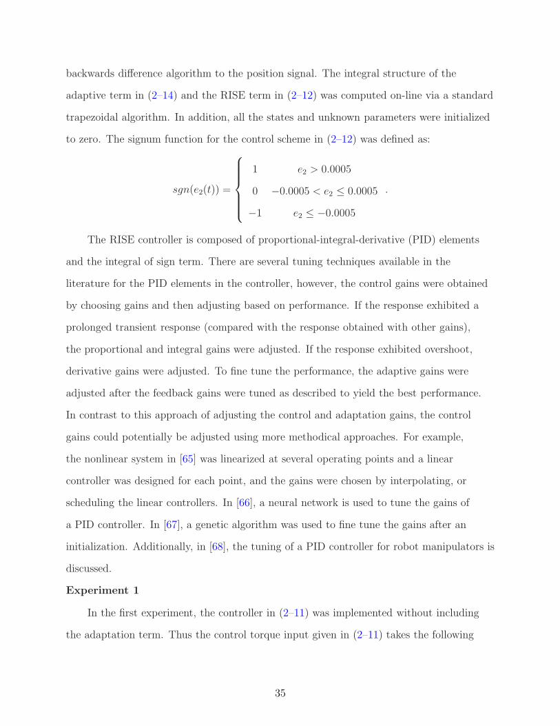
2-3 Position tracking error without the adaptive feedforward term. . . . . . . . . . . 36

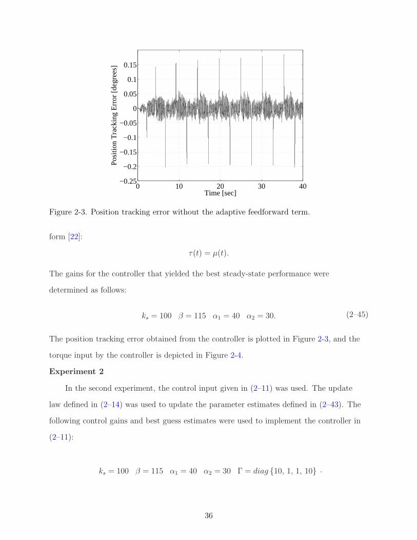
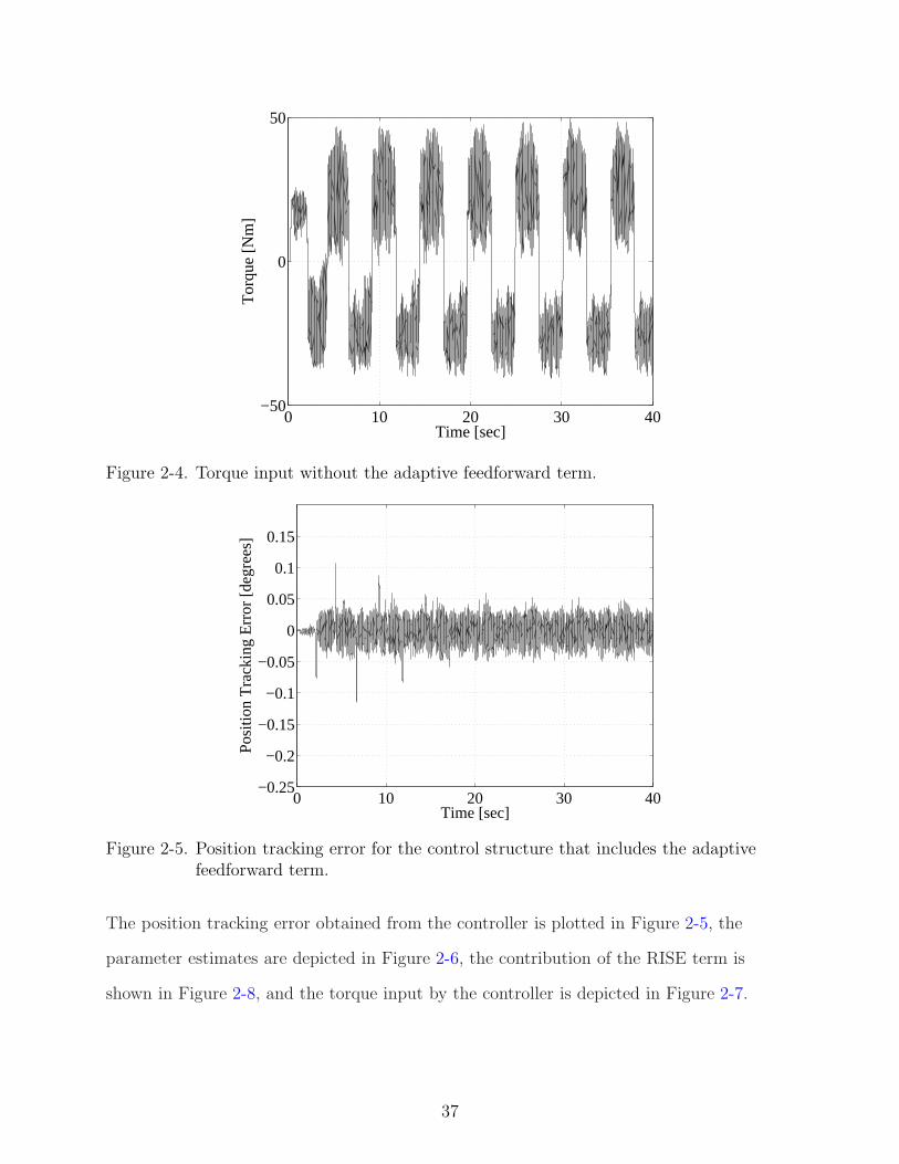
2-4 Torque input without the adaptive feedforward term. . . . . . . . . . . . . . . . 37

2-5 Position tracking error for the control structure that includes the adaptive feedforwardterm. . . . . . . . . . . . . . . . . . . . . . . . . . . . . . . . . . . . . . . . . . . 37

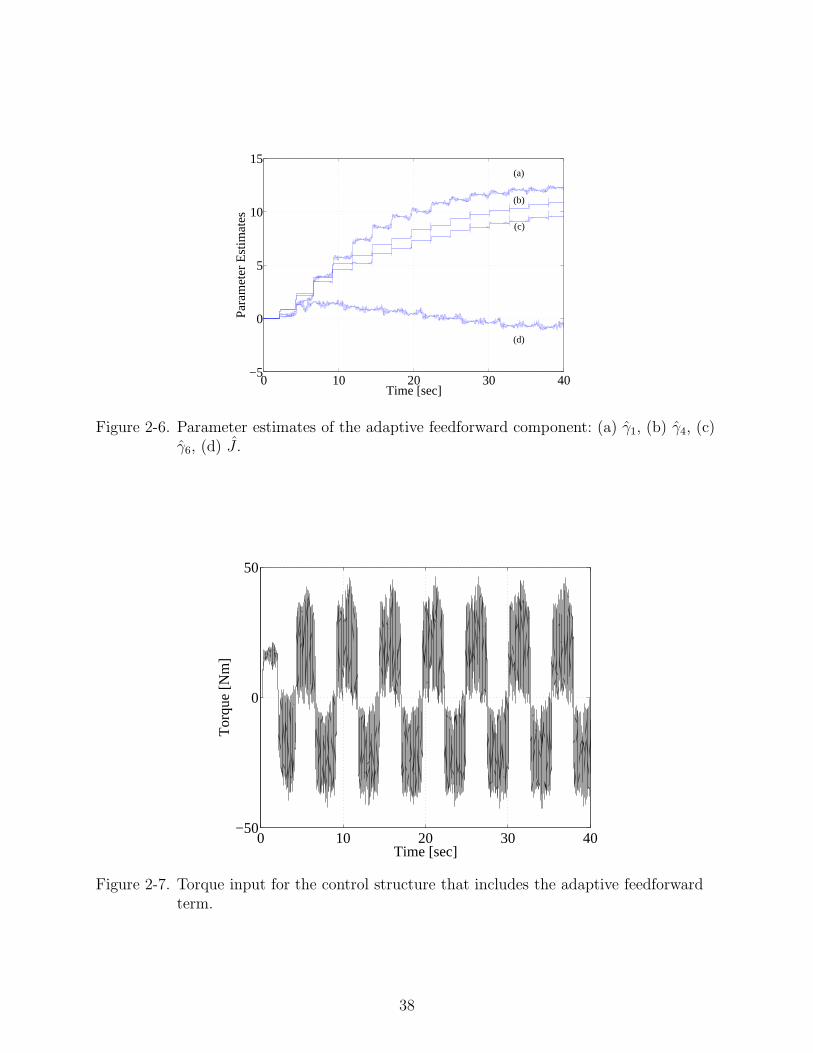
2-6 Parameter estimates of the adaptive feedforward component: (a) γ1, (b) γ4, (c)γ6, (d) J . . . . . . . . . . . . . . . . . . . . . . . . . . . . . . . . . . . . . . . . 38

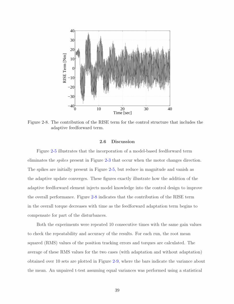
2-7 Torque input for the control structure that includes the adaptive feedforwardterm. . . . . . . . . . . . . . . . . . . . . . . . . . . . . . . . . . . . . . . . . . . 38

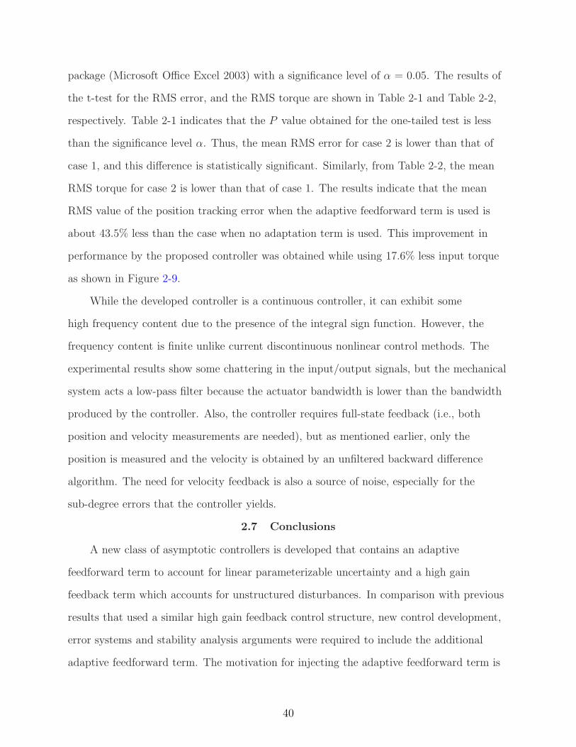
2-8 The contribution of the RISE term for the control structure that includes theadaptive feedforward term. . . . . . . . . . . . . . . . . . . . . . . . . . . . . . . 39

2-9 RMS position tracking errors and torques for the two cases - (1) without theadaptation term in the control input, (2) with the adaptation term in the controlinput. . . . . . . . . . . . . . . . . . . . . . . . . . . . . . . . . . . . . . . . . . 41

3-1 Tracking error for the RISE control law with no NN adaptation. . . . . . . . . . 59

3-2 Control torque for the RISE control law with no NN adaptation. . . . . . . . . . 60

3-3 Tracking error for the proposed RISE+NN control law. . . . . . . . . . . . . . . 60

3-4 Control torque for the proposed RISE+NN control law. . . . . . . . . . . . . . . 61

3-5 Average RMS errors (degrees) and torques (N-m). 1- RISE, 2- RISE+NN (proposed). 61

4-1 The experimental testbed consists of a two-link robot. The links are mountedon two NSK direct-drive switched reluctance motors. . . . . . . . . . . . . . . . 83

4-2 Link position tracking error with a gradient-based adaptive update law. . . . . . 87

4-3 Torque input for the modular adaptive controller with a gradient-based adaptiveupdate law. . . . . . . . . . . . . . . . . . . . . . . . . . . . . . . . . . . . . . . 87

4-4 Adaptive estimates for the gradient update law. . . . . . . . . . . . . . . . . . . 88

4-5 Link position tracking error with a least-squares adaptive update law. . . . . . . 88

9

4-6 Torque input for the modular adaptive controller with a least-squares adaptiveupdate law. . . . . . . . . . . . . . . . . . . . . . . . . . . . . . . . . . . . . . . 89

4-7 Adaptive estimates for the least squares update law. . . . . . . . . . . . . . . . 89

4-8 Link position tracking error for the modular NN controller with a gradient-basedtuning law. . . . . . . . . . . . . . . . . . . . . . . . . . . . . . . . . . . . . . . 91

4-9 Torque input for the modular NN controller with a gradient-based tuning law. . 91

4-10 Link position tracking error for the modular NN controller with a Hebbian tuninglaw. . . . . . . . . . . . . . . . . . . . . . . . . . . . . . . . . . . . . . . . . . . 92

4-11 Torque input for the modular NN controller with a Hebbian tuning law. . . . . . 92

5-1 Block diagram of the proposed RISE-based composite adaptive controller . . . . 106

5-2 Actual and desired trajectories for the proposed composite adaptive control law(RISE+CFF). . . . . . . . . . . . . . . . . . . . . . . . . . . . . . . . . . . . . . 114

5-3 Tracking error for the proposed composite adaptive control law (RISE+CFF). . 114

5-4 Prediction error for the proposed composite adaptive control law (RISE+CFF). 115

5-5 Control torque for the proposed composite adaptive control law (RISE+CFF). . 115

5-6 Contribution of the RISE term in the proposed composite adaptive control law(RISE+CFF). . . . . . . . . . . . . . . . . . . . . . . . . . . . . . . . . . . . . . 116

5-7 Adaptive estimates for the proposed composite adaptive control law (RISE+CFF).116

5-8 Average RMS errors (degrees) and torques (N-m). 1- RISE, 2- RISE+FF, 3-RISE+CFF (proposed). . . . . . . . . . . . . . . . . . . . . . . . . . . . . . . . 117

6-1 Block diagram of the proposed RISE-based composite NN controller. . . . . . . 128

6-2 Tracking error for the proposed composite adaptive control law (RISE+CNN). . 140

6-3 Prediction error for the proposed composite adaptive control law (RISE+CNN). 141

6-4 Control torque for the proposed composite adaptive control law (RISE+CNN). . 141

6-5 Average RMS errors (degrees) and torques (N-m). 1- RISE, 2- RISE+NN, 3-RISE+CNN (proposed). . . . . . . . . . . . . . . . . . . . . . . . . . . . . . . . 142

10

Abstract of Dissertation Presented to the Graduate Schoolof the University of Florida in Partial Fulfillment of theRequirements for the Degree of Doctor of Philosophy

LYAPUNOV-BASED ROBUST AND ADAPTIVE CONTROL OF NONLINEARSYSTEMS USING A NOVEL FEEDBACK STRUCTURE

By

Parag Patre

August 2009

Chair: Warren E. DixonMajor: Mechanical Engineering

The focus of this research is an examination of the interplay between different

intelligent feedforward mechanisms with a recently developed continuous robust feedback

mechanism, coined Robust Integral of the Sign of the Error (RISE), to yield asymptotic

tracking in the presence of generic disturbances. This result solves a decades long

open problem of how to obtain asymptotic stability of nonlinear systems with general

sufficiently smooth disturbances with a continuous control method. Further, it is shown

that the developed technique can be fused with other feedforward methods such as

function approximation and adaptive control methods. The addition of feedforward

elements adds system knowledge in the control structure, which heuristically, yields better

performance and reduces control effort. This heuristic notion is supported by experimental

results in this research.

One key element in the development of the novel feedforward mechanisms presented

in this dissertation is the modularity between the controller and update law. This

modularity provides flexibility in the selection of different update laws that could be

easier to implement or help to achieve faster parameter convergence and better tracking

performance.

The efficacy of the feedforward mechanisms is further enhanced by including a

prediction error in the learning process. The prediction error, which directly relates to

11

the actual function mismatch, is used along with the system tracking errors to develop a

composite adaptation law.

Each result is supported through rigorous Lyapunov-based stability proofs and

experimental demonstrations.

12

CHAPTER 1INTRODUCTION

1.1 Motivation and Problem Statement

The control of systems with uncertain nonlinear dynamics has been a decades

long mainstream area of focus. For systems with uncertainties that can be linear

parameterized, a variety of adaptive (e.g., [1–3]) feedforward controllers can be utilized

to achieve an asymptotic result. Some recent results have also targeted the application

of adaptive controllers for systems that are not linear in the parameters [4]. Learning

controllers have been developed for systems with periodic disturbances [5–7], and recent

research has focused on the use of exosystems [8–11] to compensate for disturbances

that are the solution of a linear time-invariant system with unknown coefficients. A

variety of methods have also been proposed to compensate for systems with unstructured

uncertainty including: various sliding mode controllers (e.g., [3, 12]), robust control

schemes [13], and neural network and fuzzy logic controllers [14–18]. From a review of

these approaches, a general trend is that controllers developed for systems with more

unstructured uncertainty will require more control effort (i.e., high gain or high frequency

feedback) and yield reduced performance (e.g., uniformly ultimately bounded stability).

Recently a new robust control strategy, coined Robust Integral of the Sign of the

Error (RISE) in [19, 20], was developed in [21, 22] that can accommodate for sufficiently

smooth bounded disturbances. A significant outcome of this new control structure is

that asymptotic stability is obtained despite a fairly general uncertain disturbance. This

technique was used in [23] to develop a tracking controller for nonlinear systems in the

presence of additive disturbances and parametric uncertainties under the assumption

that the disturbances are C2 with bounded time derivatives. In [24], Xian et al. utilized

this strategy to propose a new output feedback discontinuous tracking controller for a

general class of second-order nonlinear systems whose uncertain dynamics are first-order

differentiable. In [25], Zhang et al. combined the high gain feedback structure with a

13

high gain observer at the sacrifice of yielding a semi-global uniformly ultimately bounded

result. This particular high gain feedback method has also been used as an identification

technique. For example, the method has been applied to identify friction (e.g., [26]),

for range identification in perspective and paracatadioptric vision systems (e.g., [27],

[28]), and for fault detection and identification (e.g., [29]). The development in Chapter

2 is motivated by the desire to include some knowledge of the dynamics in the control

design as a means to improve the performance and reduce the control effort. Specifically,

for systems that include some dynamics that can be segregated into structured (i.e.,

linear parameterizable) and unstructured uncertainty, this chapter illustrates how a new

controller, error system, and stability analysis can be crafted to include a model-based

adaptive feedforward term in conjunction with the high gain RISE feedback technique to

yield an asymptotic tracking result.

Another learning method that has been extensively investigated by control researchers

over the last fifteen years is the use of neural networks (NNs) as a feedforward element

in the control structure. The focus on NN-based control methods is spawned from the

ramification of the fact that NNs are universal approximators [30]. That is, NNs can be

used as a black-box estimator for a general class of systems. Examples include: nonlinear

systems with parametric uncertainty that do not satisfy the linear-in-the-parameters

assumption required in most adaptive control methods; systems with deadzones or

discontinuities; and systems with backlash. Typically, NN-based controllers yield global

uniformly ultimately bounded (UUB) stability results (e.g., see [15, 31, 32] for examples

and reviews of literature) due to residual functional reconstruction inaccuracies and

an inability to compensate for some system disturbances. Motivated by the desire to

eliminate the residual steady-state errors, several researchers have obtained asymptotic

tracking results by combining the NN feedforward element with discontinuous feedback

methods such as variable structure controllers (VSC) (e.g., [33, 34]) or sliding mode (SM)

controllers (e.g., [34, 35]). A clever VSC-like controller was also proposed in [36] where

14

the controller is not initially discontinuous, but exponentially becomes discontinuous as

an exogenous control element exponentially vanishes. Well known limitations of VSC

and SM controllers include a requirement for infinite control bandwidth and chattering.

Unfortunately, ad hoc fixes for these effects result in a loss of asymptotic stability (i.e.,

UUB typically results). Motivated by issues associated with discontinuous controllers

and the typical UUB stability result, an innovative continuous NN-based controller was

recently developed in [37] to achieve partial asymptotic stability for a particular class of

systems. The result in Chapter 3 is motivated by the question: Can a NN feedforward

controller be modified by a continuous feedback element to achieve an asymptotic tracking

result for a general class of systems? Despite the pervasive development of NN controllers

in literature and the widespread use of NNs in industrial applications, the answer to

this fundamental question has remained an open problem. To provide an answer to

the fundamental motivating question, the result in Chapter 3 focuses on augmenting a

multi-layer NN-based feedforward method with the RISE control strategy

Like most of the research in adaptive control, the results in Chapter 2 and 3 exploit

Lyapunov-based techniques (i.e., the controller and the adaptive update law are designed

based on a Lyapunov analysis); however, Lyapunov-based methods restrict the design

of the adaptive update law. For example, many of the previous adaptive controllers are

restricted to utilizing gradient update laws to cancel cross terms in a Lyapunov-based

stability analysis. Gradient update laws can potentially exhibit slower parameter

convergence which could lead to a degraded transient performance of the tracking error in

comparison to other possible adaptive update laws (e.g., least-squares update law). Several

results have been developed in literature that aim to augment the typical position/velocity

tracking error-based gradient update law including: composite adaptive update laws

[3, 38, 39]; prediction error-based update laws [1, 40–43]; and various least-squares

update laws [44–46]. The adaptive update law in these results are all still designed to

cancel cross terms in the Lyapunov-based stability analysis. In contrast to these results,

15

researchers have also developed a class of modular adaptive controllers (cf. [1, 40, 42, 43])

where a feedback mechanism is used to stabilize the error dynamics provided certain

conditions are satisfied on the adaptive update law. For example, nonlinear damping

[41, 47] is typically used to yield an input-to-state stability (ISS) result with respect to

the parameter estimation error where it is assumed a priori that the update law yields

bounded parameter estimates. Often the modular adaptive control development exploits a

prediction error in the update law (e.g., see [3, 40–43]), where the prediction error is often

required to be square integrable (e.g., [40, 42, 43]). A brief survey of modular adaptive

control results is provided in [40]. Since the RISE feedback mechanism alone can yield an

asymptotic result without a feedforward component to cancel cross terms in the stability

analysis, the research in Chapter 4 is motivated by the following question: Can the RISE

control method be used to yield a new class of modular adaptive controllers?

Typical adaptive, robust adaptive, and function approximation methods and the

ones used in Chapters 2-4 use tracking error feedback to update the adaptive estimates.

As mentioned earlier, the use of the tracking error is motivated by the need for the

adaptive update law to cancel cross-terms in the closed-loop tracking error system within

a Lyapunov-based analysis. As the tracking error converges, the rate of the update

law also converges, but drawing conclusions about the convergent value (if any) of the

parameter update law is problematic. Ideally, the adaptive update law would include

some estimate of the parameter estimation error as a means to prove the parameter

estimates converge to the actual values; however, the parameter estimate error is

unknown. The desire to include some measurable form of the parameter estimation

error in the adaptation law resulted in the development of adaptive update laws that

are driven, in part, by a prediction error [3, 42, 48–50]. The prediction error is defined

as the difference between the predicted parameter estimate value and the actual system

uncertainty. Including feedback of the estimation error in the adaptive update law enables

improved parameter estimation. For example, some classic results [1, 3, 41] have proven

16

the parameter estimation error is square integrable and that the parameter estimates

may converge to the actual uncertain parameters. Since the prediction error depends

on the unmeasurable system uncertainty, the swapping lemma [3, 42, 48–50] is central

to the prediction error formulation. The swapping technique (also described as input or

torque filtering in some literature) transforms a dynamic parametric model into a static

form where standard parameter estimation techniques can be applied. In [1] and [41], a

nonlinear extension of the swapping lemma was derived, which was used to develop the

modular z-swapping and x-swapping identifiers via an input-to-state stable (ISS) controller

for systems in parametric strict feedback form. The advantages provided by prediction

error based adaptive update laws led to several results that use either the prediction

error or a composite of the prediction error and the tracking error (cf. [43, 51–56] and the

references within). Although prediction error based adaptive update laws have existed

for approximately two decades, no stability result has been developed for systems with

additive bounded disturbances. In general, the inclusion of disturbances reduces the

steady-state performance of continuous controllers to a uniformly ultimately bounded

(UUB) result. In addition to a UUB result, the inclusion of disturbances may cause

unbounded growth of the parameter estimates [57] for tracking error-based adaptive

update laws without the use of projection algorithms or other update law modifications

such as σ-modification [58]. Problems associated with the inclusion of disturbances are

magnified for control methods based on prediction error-based update laws because the

formulation of the prediction error requires the swapping (or control filtering) method.

Applying the swapping approach to dynamics with additive disturbances is problematic

because the unknown disturbance terms also get filtered and included in the filtered

control input. This problem motivates the question of how can a prediction error-based

adaptive update law be developed for systems with additive disturbances. To address this

motivating question, a general Euler-Lagrange-like MIMO system is considered in Chapter

17

5 with structured and unstructured uncertainties, and a gradient-based composite adaptive

update law is developed that is driven by both the tracking error and the prediction error.

The swapping procedure used in standard adaptive control cannot be extended to

NN controllers directly. The presence of a NN reconstruction error has impeded the

development of composite adaptation laws for NNs. Specifically, the reconstruction

error gets filtered and included in the prediction error destroying the typical prediction

error formulation. Using the techniques developed in Chapter 5, the result in Chapter 6

presents the first ever attempt to develop a prediction error-based composite adaptive NN

controller for an Euler-Lagrange second-order dynamic system using the RISE feedback.

A usual concern about the RISE feedback is the presence of high-gain and high-frequency

components in the control structure. However, in contrast to a typical widely used

discontinuous high-gain sliding mode controller, the RISE feedback offers a continuous

alternative. Moreover, the proposed control designs are not purely high gain as an

adaptive element is used as a feedforward component that learns and incorporates the

knowledge of system dynamics in the control structure.

1.2 Contributions

This research focuses on combining various feedforward terms with the RISE feedback

method for the control of uncertain nonlinear dynamic systems. The contributions of

Chapters 2-6 are as follows.

Chapter 2: Asymptotic Tracking for Systems with Structured and Unstructured

Uncertainties: The development in this chapter is motivated by the desire to include some

knowledge of the dynamics in the control design as a means to improve the performance

and reduce the control effort. Specifically, for systems that include some dynamics

that can be segregated into structured (i.e., linear parameterizable) and unstructured

uncertainty, this chapter illustrates how a new controller, error system, and stability

analysis can be crafted to include a model-based adaptive feedforward term in conjunction

with the RISE feedback technique to yield an asymptotic tracking result. This chapter

18

presents the first result that illustrates how the amalgamation of these compensation

methods can be used to yield an asymptotic result.

Chapter 3: Asymptotic Tracking for Uncertain Dynamic Systems via a Multilayer

Neural Network Feedforward and RISE Feedback Control Structure: The use of a NN as

a feedforward control element to compensate for nonlinear system uncertainties has been

investigated for over a decade. Typical NN-based controllers yield uniformly ultimately

bounded (UUB) stability results due to residual functional reconstruction inaccuracies

and an inability to compensate for some system disturbances. Several researchers have

proposed discontinuous feedback controllers (e.g., variable structure or sliding mode

controllers) to reject the residual errors and yield asymptotic results. The research in

this chapter describes how the RISE feedback term can be incorporated with a NN-based

feedforward term to achieve the first ever asymptotic tracking result. To achieve this

result, the typical stability analysis for the RISE method is modified to enable the

incorporation of the NN-based feedforward terms, and a projection algorithm is developed

to guarantee bounded NN weight estimates. Experimental results are presented to

demonstrate the performance of the proposed controller.

Chapter 4: A New Class of Modular Adaptive Controllers: A novel adaptive nonlinear

control design is developed which achieves modularity between the controller and the

adaptive update law. Modularity between the controller/update law design provides

flexibility in the selection of different update laws that could potentially be easier

to implement or used to obtain faster parameter convergence and/or better tracking

performance. For a general class of linear-in-the-parameters (LP) uncertain multi-input

multi-output systems subject to additive bounded non-LP disturbances, the developed

controller uses a model-based feedforward adaptive term in conjunction with the

RISE feedback term. Modularity in the adaptive feedforward term is made possible

by considering a generic form of the adaptive update law and its corresponding parameter

estimate. This generic form of the update law is used to develop a new closed-loop error

19

system and stability analysis that does not depend on nonlinear damping to yield the

modular adaptive control result. The result is then extended by considering uncertain

dynamic systems that are not necessarily LP, and have additive non-LP bounded

disturbances. A multilayer NN structure is used in the non-LP extension as a feedforward

element to compensate for the non-LP dynamics in conjunction with the RISE feedback

term. A NN-based controller is developed with modularity in NN weight tuning laws and

the control law. An extension is provided that describes how the control development

for the general class of systems can be applied to a class of dynamic systems modeled by

Euler-Lagrange formulation. Experimental results on a two-link robot are included to

illustrate the concept.

Chapter 5: Composite Adaptive Control for Systems with Additive Disturbances: In

a typical adaptive update law, the rate of adaptation is generally a function of the state

feedback error. Ideally, the adaptive update law would also include some feedback of the

parameter estimation error. The desire to include some measurable form of the parameter

estimation error in the adaptation law resulted in the development of composite adaptive

update laws that are functions of a prediction error and the state feedback. In all previous

composite adaptive controllers, the formulation of the prediction error is predicated on

the critical assumption that the system uncertainty is linear in the uncertain parameters

(LP uncertainty). The presence of additive disturbances that are not LP would destroy

the prediction error formulation and stability analysis arguments in previous results. In

this chapter, a new prediction error formulation is constructed through the use of the

RISE technique. The contribution of this design and associated stability analysis is that

the prediction error can be developed even with disturbances that do not satisfy the

LP assumption (e.g., additive bounded disturbances). A composite adaptive controller

is developed for a general MIMO Euler-Lagrange system with mixed structured (i.e.,

LP) and unstructured uncertainties. A Lyapunov-based stability analysis is used to

20

derive sufficient gain conditions under which the proposed controller yields semi-global

asymptotic tracking. Experimental results are presented to illustrate the approach.

Chapter 6: Composite Adaptation for NN-Based Controllers: With the motivation

of using more information to update the parameter estimates, composite adaptation

that uses both the system tracking errors and a prediction error containing parametric

information to drive the update laws, has become widespread in adaptive control

literature. However, despite its obvious benefits, composite adaptation has not been

implemented in NN-based control, primarily due to the NN reconstruction error that

destroys a typical prediction error formulation required for the composite adaptation.

This chapter presents the first ever attempt to design a composite adaptation law for

NNs by devising an innovative swapping procedure that uses the RISE feedback method.

Semi-global asymptotic tracking for the system errors is proved, while all other signals and

control input are shown to be bounded.

21

CHAPTER 2ASYMPTOTIC TRACKING FOR SYSTEMS WITH STRUCTURED AND

UNSTRUCTURED UNCERTAINTIES

2.1 Introduction

The development in this chapter is motivated by the desire to include some knowledge

of the dynamics in the control design as a means to improve the performance and reduce

the control effort. Specifically, for systems that include some dynamics that can be

segregated into structured (i.e., linear parameterizable) and unstructured uncertainty, this

chapter illustrates how a new controller and error system can be crafted to include

a model-based adaptive feedforward term in conjunction with the RISE feedback

technique to yield an asymptotic tracking result. This chapter presents the first result

that illustrates how the amalgamation of these compensation methods can be used

to yield an asymptotic result. Heuristically, the addition of the model-based adaptive

feedforward term should reduce the overall control effort because some of the disturbance

has been isolated and compensated for by a non-high gain feedforward element. Moreover,

the addition of the adaptive feedforward term injects some knowledge of the dynamics

in the control structure, which leads to improved performance. Experimental results

are presented to reinforce these heuristic notions. Specifically, the presented controller

was implemented on a simple rotating circular disk testbed and demonstrated reduced

tracking error and control effort. For this testbed, the dynamics that were included in the

feedforward term included the inertia of the linkage assembly, and the friction present in

the system.

2.2 Dynamic Model

The class of nonlinear dynamic systems considered in this manuscript is assumed to

be modeled by the following Euler-Lagrange formulation that describes the behavior of a

large class of engineering systems:

M(q)q + Vm(q, q)q +G(q) + f(q) + τd(t) = τ(t). (2–1)

22

In (2–1), M(q) ∈ Rn×n denotes a generalized inertia matrix, Vm(q, q) ∈ R

n×n denotes a

generalized centripetal-Coriolis matrix, G(q) ∈ Rn denotes a generalized gravity vector,

f(q) ∈ Rn denotes a generalized friction vector, τd (t) ∈ Rn denotes a generalized nonlinear

disturbance (e.g., unmodeled effects), τ(t) ∈ Rn represents the generalized torque input

control vector, and q(t), q(t), q(t) ∈ Rn denote the generalized link position, velocity, and

acceleration vectors, respectively. The friction term f(q) in (2–1) is assumed to have the

following form [26] and [59]:

f(q) = γ1(tanh(γ2q) − tanh(γ3q)) + γ4 tanh(γ5q) + γ6q, (2–2)

where γi ∈ R ∀i = 1, 2, ..., 6 denote unknown positive constants. The friction model

in (2–2) has the following properties: 1) it is symmetric about the origin, 2) it has a

static coefficient of friction, 3) it exhibits the Stribeck effect where the friction coefficient

decreases from the static coefficient of friction with increasing slip velocity near the origin,

4) it includes a viscous dissipation term, and 5) it has a Coulombic friction coefficient in

the absence of viscous dissipation. To a good approximation, the static friction coefficient

is given by γ1 + γ4, and the Stribeck effect is captured by tanh(γ2q) − tanh(γ3q). The

Coulombic friction coefficient is given by γ4 tanh(γ5q), and the viscous dissipation is given

by γ6q. For further details regarding the friction model, see [26] and [59]. The subsequent

development is based on the assumption that q(t) and q(t) are measurable and that M(q),

Vm(q, q), G(q), f(q), and τd(t) are unknown. The error system systems utilized in this

manuscript assume that the generalized coordinates, q (t), of the Euler-Lagrange dynamics

in (2–1) allow additive and not multiplicative errors. Moreover, the following assumptions

will be exploited in the subsequent development:

Assumption 2-1: Symmetric and Positive-Definite Inertia Matrix

The inertia matrix M(q) is symmetric, positive definite, and satisfies the following

inequality ∀ξ(t) ∈ Rn:

m1 ‖ξ‖2 ≤ ξTM(q)ξ ≤ m(q) ‖ξ‖2 (2–3)

23

where m1 ∈ R is a known positive constant, m(q) ∈ R is a known positive function, and

‖·‖ denotes the standard Euclidean norm.

Assumption 2-2: If q(t), q(t) ∈ L∞, then Vm(q, q), F (q) and G(q) are bounded.

Moreover, if q(t), q(t) ∈ L∞, then the first and second partial derivatives of the elements of

M(q), Vm(q, q), G(q) with respect to q (t) exist and are bounded, and the first and second

partial derivatives of the elements of Vm(q, q), F (q) with respect to q(t) exist and are

bounded.

Assumption 2-3: The nonlinear disturbance term and its first two time derivatives, i.e.

τd (t) , τd (t) , τd (t) are bounded by known constants.

Assumption 2-4: The desired trajectory is designed such that q(i)d (t) ∈ Rn (i = 0, 1, ..., 4)

exist and are bounded.

2.3 Error System Development

The control objective is to ensure that the system tracks a desired time-varying

trajectory despite structured and unstructured uncertainties in the dynamic model. To

quantify this objective, a position tracking error, denoted by e1(t) ∈ Rn, is defined as

e1 = qd − q. (2–4)

To facilitate the subsequent analysis, filtered tracking errors, denoted by e2(t), r(t) ∈ Rn,

are also defined as

e2 = e1 + α1e1 (2–5)

r = e2 + α2e2, (2–6)

where α1, α2 ∈ R denote positive constants. The subsequent development is based on the

assumption that q (t) and q (t) are measurable, so the filtered tracking error r(t) is not

measurable since the expression in (2–6) depends on q(t).

24

The open-loop tracking error system can be developed by premultiplying (2–6) by

M(q) and utilizing the expressions in (2–1)-(2–5) to obtain the following expression:

M(q)r = Ydθ + S +Wd + τd(t) − τ(t), (2–7)

where Yd (qd, qd, qd) θ ∈ Rn is defined as

Ydθ , M(qd)qd + Vm(qd, qd)qd +G(qd) + γ1 (tanh (γ2qd) − tanh (γ3qd)) (2–8)

+ γ4 tanh (γ5qd) + γ6qd.

In (2–8), θ ∈ Rp contains the constant unknown system parameters, Yd (qd, qd, qd) ∈ Rn×p

is the desired regression matrix that contains known functions of the desired link position,

velocity, and acceleration, qd (t) , qd (t) , qd (t) ∈ Rn, respectively, and γ2, γ3, γ5 ∈ R are

the best guess estimates for γ2, γ3, and γ5, respectively. In (2–7), the auxiliary function

S (q, q, qd, qd, qd) ∈ Rn is defined as

S , M (q) (α1e1 + α2e2) +M (q) qd −M(qd)qd + Vm(q, q)q − Vm(qd, qd)qd +G(q) −G(qd)

+ γ6q − γ6qd + γ4 tanh (γ5q) − γ4 tanh (γ5qd) + γ1 (tanh (γ2q) − tanh (γ3q)) (2–9)

− γ1 (tanh (γ2qd) − tanh (γ3qd)) ,

and the auxiliary function Wd(qd) ∈ Rn is defined as

Wd , γ4 tanh (γ5qd) − γ4 tanh (γ5qd) + γ1 (tanh (γ2qd) − tanh (γ3qd)) (2–10)

− γ1 (tanh (γ2qd) − tanh (γ3qd)) .

Based on the expression in (2–7), the control torque input is designed as

τ = Ydθ + µ. (2–11)

In (2–11), µ(t) ∈ Rn denotes the RISE term defined as

µ(t) , (ks + 1)e2(t) − (ks + 1)e2(0) +

∫ t

0

[(ks + 1)α2e2(σ) + βsgn(e2(σ))]dσ, (2–12)

25

where ks, β ∈ R are positive, constant control gains, and θ(t) ∈ Rp denotes a parameter

estimate vector generated on-line according to the following update law:

·

θ = ΓY Td r (2–13)

with Γ ∈ Rp×p being a known, constant, diagonal, positive-definite adaptation gain matrix.

Since Yd(t) is only a function of the known desired time varying trajectory, (2–13) can be

integrated by parts as follows:

θ(t) = θ(0) + ΓY Td e2(σ)

∣

∣

∣

t

0− Γ

∫ t

0

Y Td e2(σ) − α2Y

Td e2(σ)

dσ (2–14)

so that the parameter estimate vector θ(t) implemented in (2–11) does not depend on the

unmeasurable signal r(t).

Remark 2.1. The control design in (2–11) is similar to the results in [22]. However,

previous designs based on [22] could only compensate for uncertainty in the system through

the high gain RISE feedback term µ(t). Through the new development presented in the

current result, an adaptive feedforward term can also be used to compensate for system

uncertainty. This flexibility presents a significant advantage because it allows more system

dynamics to be incorporated in the control design. Specifically, if some of the system

uncertainty can be segregated into a linear parameterizable form, then the model-based

adaptive feedforward term can be injected to compensate for the uncertainty instead of

just relying on the non-model based high gain RISE feedback term. Heuristically, this

contribution should improve the tracking performance and reduce the control effort.

Experimental results on a simple one-link robot manipulator provide some validation of this

heuristic idea.

The closed-loop tracking error system can be developed by substituting (2–11) into

(2–7) as

M(q)r = Ydθ + S +Wd + τd − µ(t), (2–15)

26

where θ(t) ∈ Rp represents the parameter estimation error vector defined as

θ = θ − θ. (2–16)

To facilitate the subsequent stability analysis (and to illustrate some insight into the

structure of the design for µ(t)), the time derivative of (2–15) is determined as

M(q)r = −1

2M(q)r + Ydθ + N (t) +Nd (t) − µ(t) − e2, (2–17)

where the unmeasurable auxiliary term N(e1, e2, r) ∈ Rn is defined as

N(t) , −YdΓYTd r + S −

1

2M(q)r + e2, (2–18)

where (2–13) was used. In (2–17), the unmeasurable auxiliary term Nd(qd, qd, qd) ∈ Rn is

defined as

Nd (t) , Wd + τd. (2–19)

The time derivative of (2–12) is given as

µ(t) = (ks + 1)r + βsgn(e2). (2–20)

In a similar manner as in [60], the Mean Value Theorem can be used to develop the

following upper bound1

∥

∥

∥N(t)

∥

∥

∥≤ ρ (‖z‖) ‖z‖ , (2–21)

where z(t) ∈ R3n is defined as

z(t) ,[

eT1 eT

2 rT]T. (2–22)

The following inequalities can be developed based on the expression in (2–19) and its time

derivative:

‖Nd(t)‖ ≤ ζNd

∥

∥

∥Nd(t)

∥

∥

∥≤ ζNd2

, (2–23)

1 See Lemma 1 of the Appendix for the proof of the inequality in (2–21).

27

where ζNd, ζNd2

∈ R are known positive constants.

2.4 Stability Analysis

Theorem 2-1: The controller given in (2–11), (2–12), and (2–14) ensures that all

system signals are bounded under closed-loop operation and that the position tracking

error is regulated in the sense that

‖e1(t)‖ → 0 as t→ ∞

provided the control gain ks introduced in (2–12) is selected sufficiently large based on the

initial conditions of the system (see the subsequent proof for details), α1, α2 are selected

according to the following sufficient condition

α1 >1

2, α2 > 1 (2–24)

and β is selected according to the following sufficient condition

β > ζNd+

1

α2ζNd2

(2–25)

where ζNdand ζNd2

are introduced in (2–23).

Proof: Let D ⊂ R3n+p+1 be a domain containing y(t) = 0, where y(t) ∈ R3n+p+1 is

defined as

y(t) ,

[

zT (t) θT (t)√

P (t)]T

(2–26)

and the auxiliary function P (t) ∈ R is defined as

P (t) , βn∑

i=1

|e2i(0)| − e2(0)TNd(0) −

∫ t

0

L(τ)dτ (2–27)

where the subscript i = 1, 2, .., n denotes the ith element of the vector. In (2–27), the

auxiliary function L(t) ∈ R is defined as

L(t) , rT (Nd(t) − βsgn(e2)) . (2–28)

28

The derivative P (t) ∈ R can be expressed as

P (t) = −L(t) = −rT (Nd(t) − βsgn(e2)). (2–29)

Provided the sufficient condition introduced in (2–25) is satisfied, the following inequality

can be obtained2 :∫ t

0

L(τ)dτ ≤ βn∑

i=1

|e2i(0)| − e2(0)TNd(0). (2–30)

Hence, (2–30) can be used to conclude that P (t) ≥ 0.

Let V (y, t) : D× [0,∞) → R be a continuously differentiable, positive definite function

defined as

V (y, t) , eT1 e1 +

1

2eT2 e2 +

1

2rTM(q)r + P +

1

2θT Γ−1θ (2–31)

which satisfies the following inequalities:

U1(y) ≤ V (y, t) ≤ U2(y) (2–32)

provided the sufficient condition introduced in (2–25) is satisfied. In (2–32), the

continuous, positive definite functions U1(y), U2(y) ∈ R are defined as

U1(y) , η1 ‖y‖2 U2(y) , η2(q) ‖y‖

2 (2–33)

where η1, η2(q) ∈ R are defined as

η1 ,1

2min

1, m1, λmin

Γ−1

η2(q) , max

1

2m(q),

1

2λmax

Γ−1

, 1

where m1, m(q) are introduced in (2–3) and λmin · , λmax · denote the minimum and

maximum eigenvalues, respectively, of the argument. After taking the time derivative of

2 The inequality in (2–30) can be obtained in a similar manner as in Lemma 2 of theAppendix.

29

(2–31), V (y, t) can be expressed as

V (y, t) = rTM(q)r +1

2rTM(q)r + eT

2 e2 + 2eT1 e1 + P − θT Γ−1

·

θ.

Remark 2.2. From (2–17), (2–27) and (2–28), some of the differential equations de-

scribing the closed-loop system for which the stability analysis is being performed have

discontinuous right-hand sides as

Mr = −1

2M(q)r + Ydθ + N (t) +Nd (t) − (ks + 1)r − β1sgn(e2) − e2 (2–34)

P (t) = −L(t) = −rT (Nd(t) − βsgn(e2)) (2–35)

Let f (y, t) ∈ Rn+1 denote the right-hand side of (2–34)–(2–35). Since the subsequent

analysis requires that a solution exists for y = f (y, t), it is important to show the existence

and uniqueness of the solution to (2–34)–(2–35). As described in [13, 61], the existence

of Filippov’s generalized solution can be established for (2–34)–(2–35). First, note that

f (y, t) is continuous except in the set (y, t) |e2 = 0. Let F (y, t) be a compact, convex,

upper semicontinuous set-valued map that embeds the differential equation y = f (y, t)

into the differential inclusions y ∈ F (y, t). From Theorem 27 of [13], an absolute

continuous solution exists to y ∈ F (y, t) that is a generalized solution to y = f (y, t).

A common choice for F (y, t) that satisfies the above conditions is the closed convex hull

of f (y, t) [13, 61]. A proof that this choice for F (y, t) is upper semicontinuous is given

in [62]. Moreover, note that the differential equation describing the original closed-loop

system (i.e., after substituting (2–11) into (2–1)) has a continuous right-hand side; thus,

satisfying the condition for existence of classical solutions. Similar arguments are used for

all the results in this dissertation.

After utilizing (2–5), (2–6), (2–13), (2–17), (2–20), and (2–29), V (y, t) can be

simplified as

V (y, t) = rT N(t) − (ks + 1) ‖r‖2 − α2 ‖e2‖2 − 2α1 ‖e1‖

2 + 2eT2 e1. (2–36)

30

Because eT2 (t)e1(t) can be upper bounded as

eT2 e1 ≤

1

2‖e1‖

2 +1

2‖e2‖

2

V (y, t) can be upper bounded using the squares of the components of z(t) as follows:

V (y, t) ≤ rT N(t) − (ks + 1) ‖r‖2 − α2 ‖e2‖2 − 2α1 ‖e1‖

2 + ‖e1‖2 + ‖e2‖

2 .

By using (2–21), the expression in (2–36) can be rewritten as follows:

V (y, t) ≤ −η3 ‖z‖2 −

(

ks ‖r‖2 − ρ(‖z‖) ‖r‖ ‖z‖

)

(2–37)

where η3 , min2α1 − 1, α2 − 1, 1, and the bounding function ρ(‖z‖) ∈ R is a positive,

globally invertible, nondecreasing function; hence, α1, and α2 must be chosen according to

the sufficient conditions in (2–24). After completing the squares for the parenthetic terms

in (2–37), the following expression can be obtained:

V (y, t) ≤ −η3 ‖z‖2 +

ρ2(‖z‖) ‖z‖2

4ks

. (2–38)

The expression in (2–38) can be further upper bounded by a continuous, positive

semi-definite function

V (y, t) ≤ −U(y) = −c ‖z‖2 ∀y ∈ D (2–39)

for some positive constant c ∈ R, where

D ,

y ∈ R3n+p+1 | ‖y‖ ≤ ρ−1

(

2√

η3ks

)

.

Larger values of k will expand the size of the domain D. The inequalities in (2–32) and

(2–39) can be used to show that V (y, t) ∈ L∞ in D; hence, e1(t), e2(t), r(t), and θ(t) ∈ L∞

in D. Given that e1(t), e2(t), and r(t) ∈ L∞ in D, standard linear analysis methods can

be used to prove that e1(t), e2(t) ∈ L∞ in D from (2–5) and (2–6). Since θ ∈ Rp contains

the constant unknown system parameters and θ(t) ∈ L∞ in D, (2–16) can be used to

31

prove that θ(t) ∈ L∞ in D. Since e1(t), e2(t), r(t) ∈ L∞ in D, the assumption that qd(t),

qd(t), qd(t) exist and are bounded can be used along with (2–4)-(2–6) to conclude that

q(t), q(t), q(t) ∈ L∞ in D. The assumption that qd(t), qd(t), qd(t),...q d(t),

....q d(t) exist and

are bounded along with (2–8) can be used to show that Yd (qd, qd, qd), Yd (qd, qd, qd,...q d),

and Yd (qd, qd, qd,...q d,

....q d) ∈ L∞ in D. Since q(t), q(t) ∈ L∞ in D, Assumption 2-2 can be

used to conclude that M(q), Vm(q, q), G(q), and F (q) ∈ L∞ in D. Thus from (2–1) and

Assumption 2-3, we can show that τ(t) ∈ L∞ in D. Given that r(t) ∈ L∞ in D, (2–20) can

be used to show that µ(t) ∈ L∞ in D. Since q(t), q(t) ∈ L∞ in D, Assumption 2-2 can be

used to show that Vm(q, q), G(q), F (q) and M(q) ∈ L∞ in D; hence, (2–17) can be used to

show that r(t) ∈ L∞ in D. Since e1(t), e2(t), r(t) ∈ L∞ in D, the definitions for U(y) and

z(t) can be used to prove that U(y) is uniformly continuous in D.

Let S ⊂ D denote a set defined as follows:3

S ,

y(t) ∈ D | U (y(t)) < η1

(

ρ−1(

2√

η3ks

))2

. (2–40)

Theorem 8.4 of [63] can now be invoked to state that

c ‖z(t)‖2 → 0 as t→ ∞ ∀y(0) ∈ S. (2–41)

Based on the definition of z(t), (2–41) can be used to show that

‖e1(t)‖ → 0 as t→ ∞ ∀y(0) ∈ S.

2.5 Experimental Results

The testbed depicted in Figure 2-1 was used to implement the developed controller.

The testbed consists of a circular disc of unknown inertia mounted on a NSK direct-drive

3 The region of attraction in (2–40) can be made arbitrarily large to include any initialconditions by increasing the control gain ks (i.e., a semi-global type of stability result) [22].

32

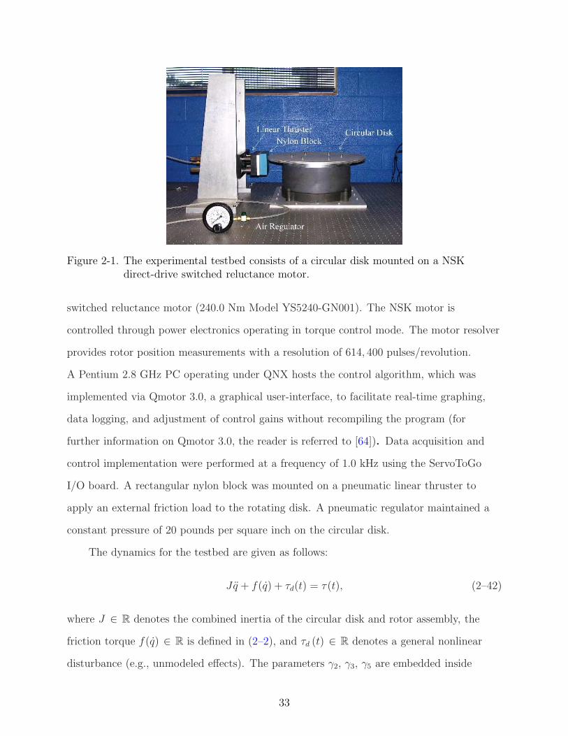
Figure 2-1. The experimental testbed consists of a circular disk mounted on a NSKdirect-drive switched reluctance motor.

switched reluctance motor (240.0 Nm Model YS5240-GN001). The NSK motor is

controlled through power electronics operating in torque control mode. The motor resolver

provides rotor position measurements with a resolution of 614, 400 pulses/revolution.

A Pentium 2.8 GHz PC operating under QNX hosts the control algorithm, which was

implemented via Qmotor 3.0, a graphical user-interface, to facilitate real-time graphing,

data logging, and adjustment of control gains without recompiling the program (for

further information on Qmotor 3.0, the reader is referred to [64]). Data acquisition and

control implementation were performed at a frequency of 1.0 kHz using the ServoToGo

I/O board. A rectangular nylon block was mounted on a pneumatic linear thruster to

apply an external friction load to the rotating disk. A pneumatic regulator maintained a

constant pressure of 20 pounds per square inch on the circular disk.

The dynamics for the testbed are given as follows:

Jq + f(q) + τd(t) = τ(t), (2–42)

where J ∈ R denotes the combined inertia of the circular disk and rotor assembly, the

friction torque f(q) ∈ R is defined in (2–2), and τd (t) ∈ R denotes a general nonlinear

disturbance (e.g., unmodeled effects). The parameters γ2, γ3, γ5 are embedded inside

33

0 5 10 15 20 25 30 35 40−50

0

50

Time [sec]

Des

ired

Tra

ject

ory

[deg

rees

]

Figure 2-2. Desired trajectory used for the experiment.

the nonlinear hyperbolic tangent functions and hence cannot be linearly parameterized.

Since these parameters cannot be compensated for by an adaptive algorithm, best-guess

estimates γ2 = 50, γ3 = 1, γ5 = 50 are used. The values for γ2, γ3, γ5 are based on

previous experiments concerned with friction identification. Significant errors in these

static estimates could degrade the performance of the system. The control torque input

τ(t) is given by (2–11), where Yd (qd, qd) ∈ R1×4 is the regression matrix defined as

Yd ,

[

qd tanh (γ2qd) − tanh (γ3qd) tanh (γ5qd) qd

]

,

and θ (t) ∈ R4 is the vector consisting of the unknown parameters defined as

θ ,

[

J γ1 γ4 γ6

]T

. (2–43)

The parameter estimates vector in (2–43) is generated on-line using the adaptive update

law in (2–14). The desired link trajectory (see Figure 2-2) was selected as follows (in

degrees):

qd(t) = 45.0 sin(1.2t)(1 − exp(−0.01t3)). (2–44)

For all experiments, the rotor velocity signal is obtained by applying a standard

34

backwards difference algorithm to the position signal. The integral structure of the

adaptive term in (2–14) and the RISE term in (2–12) was computed on-line via a standard

trapezoidal algorithm. In addition, all the states and unknown parameters were initialized

to zero. The signum function for the control scheme in (2–12) was defined as:

sgn(e2(t)) =

1 e2 > 0.0005

0 −0.0005 < e2 ≤ 0.0005

−1 e2 ≤ −0.0005

.

The RISE controller is composed of proportional-integral-derivative (PID) elements

and the integral of sign term. There are several tuning techniques available in the

literature for the PID elements in the controller, however, the control gains were obtained

by choosing gains and then adjusting based on performance. If the response exhibited a

prolonged transient response (compared with the response obtained with other gains),

the proportional and integral gains were adjusted. If the response exhibited overshoot,

derivative gains were adjusted. To fine tune the performance, the adaptive gains were

adjusted after the feedback gains were tuned as described to yield the best performance.

In contrast to this approach of adjusting the control and adaptation gains, the control

gains could potentially be adjusted using more methodical approaches. For example,

the nonlinear system in [65] was linearized at several operating points and a linear

controller was designed for each point, and the gains were chosen by interpolating, or

scheduling the linear controllers. In [66], a neural network is used to tune the gains of

a PID controller. In [67], a genetic algorithm was used to fine tune the gains after an

initialization. Additionally, in [68], the tuning of a PID controller for robot manipulators is

discussed.

Experiment 1

In the first experiment, the controller in (2–11) was implemented without including

the adaptation term. Thus the control torque input given in (2–11) takes the following

35

0 10 20 30 40−0.25

−0.2

−0.15

−0.1

−0.05

0

0.05

0.1

0.15

Pos

ition

Tra

ckin

g E

rror

[deg

rees

]

Time [sec]

Figure 2-3. Position tracking error without the adaptive feedforward term.

form [22]:

τ(t) = µ(t).

The gains for the controller that yielded the best steady-state performance were

determined as follows:

ks = 100 β = 115 α1 = 40 α2 = 30. (2–45)

The position tracking error obtained from the controller is plotted in Figure 2-3, and the

torque input by the controller is depicted in Figure 2-4.

Experiment 2

In the second experiment, the control input given in (2–11) was used. The update

law defined in (2–14) was used to update the parameter estimates defined in (2–43). The

following control gains and best guess estimates were used to implement the controller in

(2–11):

ks = 100 β = 115 α1 = 40 α2 = 30 Γ = diag 10, 1, 1, 10 .

36

0 10 20 30 40−50

0

50

Tor

que

[Nm

]

Time [sec]

Figure 2-4. Torque input without the adaptive feedforward term.

0 10 20 30 40−0.25

−0.2

−0.15

−0.1

−0.05

0

0.05

0.1

0.15

Pos

ition

Tra

ckin

g E

rror

[deg

rees

]

Time [sec]

Figure 2-5. Position tracking error for the control structure that includes the adaptivefeedforward term.

The position tracking error obtained from the controller is plotted in Figure 2-5, the

parameter estimates are depicted in Figure 2-6, the contribution of the RISE term is

shown in Figure 2-8, and the torque input by the controller is depicted in Figure 2-7.

37

0 10 20 30 40−5

0

5

10

15

Par

amet

er E

stim

ates

Time [sec]

(d)

(c)

(b)

(a)

Figure 2-6. Parameter estimates of the adaptive feedforward component: (a) γ1, (b) γ4, (c)γ6, (d) J .

0 10 20 30 40−50

0

50

Tor

que

[Nm

]

Time [sec]

Figure 2-7. Torque input for the control structure that includes the adaptive feedforwardterm.

38

0 10 20 30 40−40

−30

−20

−10

0

10

20

30

40

RIS

E T

erm

[Nm

]

Time [sec]

Figure 2-8. The contribution of the RISE term for the control structure that includes theadaptive feedforward term.

2.6 Discussion

Figure 2-5 illustrates that the incorporation of a model-based feedforward term

eliminates the spikes present in Figure 2-3 that occur when the motor changes direction.

The spikes are initially present in Figure 2-5, but reduce in magnitude and vanish as

the adaptive update converges. These figures exactly illustrate how the addition of the

adaptive feedforward element injects model knowledge into the control design to improve

the overall performance. Figure 2-8 indicates that the contribution of the RISE term

in the overall torque decreases with time as the feedforward adaptation term begins to

compensate for part of the disturbances.

Both the experiments were repeated 10 consecutive times with the same gain values

to check the repeatability and accuracy of the results. For each run, the root mean

squared (RMS) values of the position tracking errors and torques are calculated. The

average of these RMS values for the two cases (with adaptation and without adaptation)

obtained over 10 sets are plotted in Figure 2-9, where the bars indicate the variance about

the mean. An unpaired t-test assuming equal variances was performed using a statistical

39

package (Microsoft Office Excel 2003) with a significance level of α = 0.05. The results of

the t-test for the RMS error, and the RMS torque are shown in Table 2-1 and Table 2-2,

respectively. Table 2-1 indicates that the P value obtained for the one-tailed test is less

than the significance level α. Thus, the mean RMS error for case 2 is lower than that of

case 1, and this difference is statistically significant. Similarly, from Table 2-2, the mean

RMS torque for case 2 is lower than that of case 1. The results indicate that the mean

RMS value of the position tracking error when the adaptive feedforward term is used is

about 43.5% less than the case when no adaptation term is used. This improvement in

performance by the proposed controller was obtained while using 17.6% less input torque

as shown in Figure 2-9.

While the developed controller is a continuous controller, it can exhibit some

high frequency content due to the presence of the integral sign function. However, the

frequency content is finite unlike current discontinuous nonlinear control methods. The

experimental results show some chattering in the input/output signals, but the mechanical

system acts a low-pass filter because the actuator bandwidth is lower than the bandwidth

produced by the controller. Also, the controller requires full-state feedback (i.e., both

position and velocity measurements are needed), but as mentioned earlier, only the

position is measured and the velocity is obtained by an unfiltered backward difference

algorithm. The need for velocity feedback is also a source of noise, especially for the

sub-degree errors that the controller yields.

2.7 Conclusions

A new class of asymptotic controllers is developed that contains an adaptive

feedforward term to account for linear parameterizable uncertainty and a high gain

feedback term which accounts for unstructured disturbances. In comparison with previous

results that used a similar high gain feedback control structure, new control development,

error systems and stability analysis arguments were required to include the additional

adaptive feedforward term. The motivation for injecting the adaptive feedforward term is

40

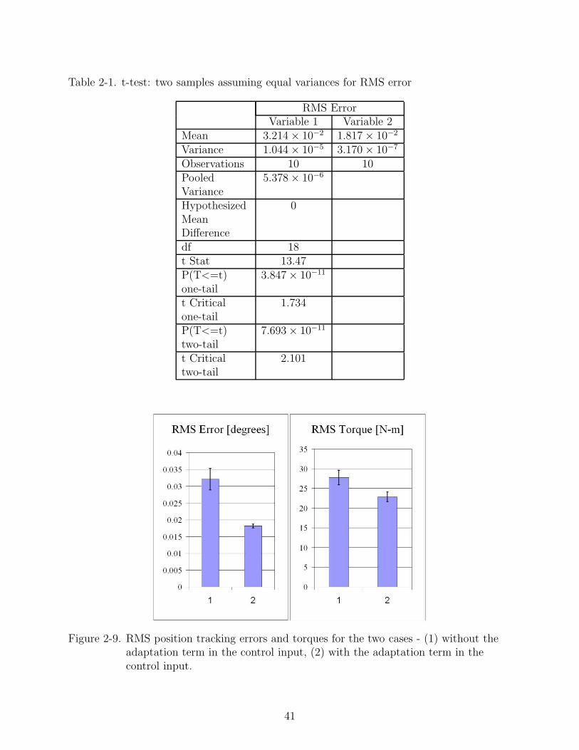
Table 2-1. t-test: two samples assuming equal variances for RMS error

RMS ErrorVariable 1 Variable 2

Mean 3.214 × 10−2 1.817 × 10−2

Variance 1.044 × 10−5 3.170 × 10−7

Observations 10 10PooledVariance

5.378 × 10−6

HypothesizedMeanDifference

0

df 18t Stat 13.47P(T<=t)one-tail

3.847 × 10−11

t Criticalone-tail

1.734

P(T<=t)two-tail

7.693 × 10−11

t Criticaltwo-tail

2.101

Figure 2-9. RMS position tracking errors and torques for the two cases - (1) without theadaptation term in the control input, (2) with the adaptation term in thecontrol input.

41

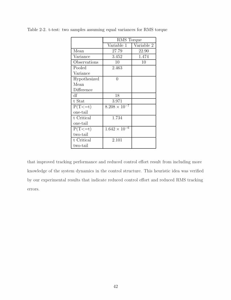
Table 2-2. t-test: two samples assuming equal variances for RMS torque

RMS TorqueVariable 1 Variable 2

Mean 27.79 22.90Variance 3.452 1.474Observations 10 10PooledVariance

2.463

HypothesizedMeanDifference

0

df 18t Stat 3.971P(T<=t)one-tail

8.208 × 10−7

t Criticalone-tail

1.734

P(T<=t)two-tail

1.642 × 10−6

t Criticaltwo-tail

2.101

that improved tracking performance and reduced control effort result from including more

knowledge of the system dynamics in the control structure. This heuristic idea was verified

by our experimental results that indicate reduced control effort and reduced RMS tracking

errors.

42

CHAPTER 3ASYMPTOTIC TRACKING FOR UNCERTAIN DYNAMIC SYSTEMS VIA A

MULTILAYER NEURAL NETWORK FEEDFORWARD AND RISE FEEDBACKCONTROL STRUCTURE

3.1 Introduction

The contribution in this chapter is motivated by the question: Can a NN feedforward

controller be modified by a continuous feedback element to achieve an asymptotic tracking

result for a general class of systems? Despite the pervasive development of NN controllers

in literature and the widespread use of NNs in industrial applications, the answer to this

fundamental question has remained an open problem.

To provide an answer to the fundamental motivating question, the result in this

chapter focuses on augmenting a multi-layer NN-based feedforward method with a recently

developed [21] high gain control strategy coined the Robust Integral of the Sign of the

Error (RISE) in [19, 20]. The RISE control structure is advantageous because it is a

differentiable control method that can compensate for additive system disturbances and

parametric uncertainties under the assumption that the disturbances are C2 with bounded

time derivatives. Due to the advantages of the RISE control structure a flurry of results

have recently been developed (e.g., [22, 23, 25–27]).

A RISE feedback controller can be directly applied to yield asymptotic stability for

the class of systems described in this chapter. However, the RISE method is a high-gain

feedback tool, and hence, clear motivation exists (as with any other feedback controller)

to combine a feedforward control element with the feedback controller for potential gains

such as improved transient and steady-state performance, and reduced control effort.

That is, it is well accepted that a feedforward component can be used to cancel out some

dynamic effects without relying on high-gain feedback. Given this motivation, some results

have already been developed that combine the RISE feedback element with feedforward

terms. In [60], a remark is provided regarding the use of a constant best-guess feedforward

component in conjunction with the RISE method to yield a UUB result. In [19, 20], the

43

RISE feedback controller was combined with a standard gradient feedforward term for

systems that satisfy the linear-in-the-parameters assumption. The experimental results

in [19] illustrate significant improvement in the root-mean-squared tracking error with

reduced root-mean-squared control effort. However, for systems that do not satisfy the

linear-in-the-parameters assumption, motivation exists to combine the RISE controller

with a new feedforward method such as the NN.

To blend the NN and RISE methods, several technical challenges must be addressed.

One (lesser) challenge is that the NN must be constructed in terms of the desired

trajectory instead of the actual trajectory (i.e., a DCAL-based NN structure [36]) to

remove the dependence on acceleration. The development of a DCAL-based NN structure

is challenging for a multi-layer NN because the adaptation law for the weights is required

to be state-dependent. Straightforward application of the RISE method would yield an

acceleration dependent adaptation law. One method to resolve this issue is to use a “dirty

derivative” (as in the UUB result in [69]; see also [25]). In lieu of a dirty derivative, the

result in this chapter uses a Lyapunov-based stability analysis approach for the design

of an adaptation law that is only velocity dependent. In comparison with the efforts in

[19, 20], a more significant challenge arises from the fact that since a multi-layer NN

includes the first layer weight estimate inside of a nonlinear activation function, the

previous methods (e.g., [19, 20]) can not be applied. That is, because of the unique

manner in which the NN weight estimates appear, the stability analysis and sufficient

conditions developed in previous works are violated. Previous RISE methods have

a restriction (encapsulated by a sufficient gain condition) that terms in the stability

analysis that are upper bounded by a constant must also have time derivatives that are

upper bounded by a constant (these terms are usually denoted by Nd (t) in RISE control

literature, see [60]). The norm of the NN weight estimates can be bounded by a constant

(due to a projection algorithm) but the time derivative is state-dependent (i.e., the norm

of Nd (t) can be bounded by a constant but the norm of Nd (t) is state dependent). To

44

address this issue, modified RISE stability analysis techniques are developed that result

in modified (but not more restrictive) sufficient gain conditions. By addressing this issue

through stability analysis methods, the standard NN weight adaptation law does not need

to be modified. Through unique modifications to the stability analysis that enable the

RISE feedback controller to be combined with the NN feedforward term, the result in this

chapter provides an affirmative answer for the first time to the aforementioned motivating

question.

Since the NN and the RISE control structures are model independent (black box)

methods, the resulting controller is a universal reusable controller [36] for continuous

systems. Because of the manner in which the RISE technique is blended with the

NN-based feedforward method, the structure of the NN is not altered from textbook

examples [15] and can be considered a somewhat modular element in the control structure.

Hence, the NN weights and thresholds are automatically adjusted on-line, with no

off-line learning phase required. Compared to standard adaptive controllers, the current

asymptotic result does not require linearity in the parameters or the development and

evaluation of a regression matrix.

For systems with linear-in-the-parameters uncertainty, an adaptive feedforward

controller has the desirable characteristics that the controller is continuous, can be

proven to yield global asymptotic tracking, and includes the specific dynamics of the

system in the feedforward path. Continuous feedback NN controllers don’t include the

specific dynamics in a regression matrix and have a degraded steady-state stability

result (i.e., UUB tracking); however, they can be applied when the uncertainty in

the system is unmodeled, can not be linearly parameterized, or the development and

implementation of a regression matrix is impractical. Sliding mode feedback NN

controllers have the advantage that they can achieve global asymptotic tracking at the

expense of implementing a discontinuous feedback controller (i.e., infinite bandwidth,

exciting structural modes, etc.). In comparison to these controllers, the development

45

in this chapter has the advantage of asymptotic tracking with a continuos feedback

controller for a general class of uncertainty; however, these advantages are at the expense

of semi-global tracking instead of the typical global tracking results.

3.2 Dynamic Model

The dynamic model and its properties are the same as in Chapter 2; however, the

dynamics are not assumed to satisfy the linear-in-the-parameters assumption.

3.3 Control Objective

The control objective is to ensure that the system tracks a desired time-varying

trajectory, denoted by qd(t) ∈ Rn, despite uncertainties in the dynamic model. To quantify

this objective, a position tracking error, denoted by e1(t) ∈ Rn, is defined as

e1 , qd − q. (3–1)

To facilitate the subsequent analysis, filtered tracking errors, denoted by e2(t), r(t) ∈ Rn,

are also defined as

e2 , e1 + α1e1 (3–2)

r , e2 + α2e2 (3–3)

where α1, α2 ∈ R denote positive constants. The filtered tracking error r(t) is not

measurable since the expression in (3–3) depends on q(t).

3.4 Feedforward NN Estimation

NN-based estimation methods are well suited for control systems where the dynamic

model contains unstructured nonlinear disturbances as in (2–1). The main feature that

empowers NN-based controllers is the universal approximation property. Let S be a

compact simply connected set of RN1+1. With map f : S → R

n, define Cn (S) as the

space where f is continuous. There exist weights and thresholds such that some function

f(x) ∈ Cn (S) can be represented by a three-layer NN as [15, 32]

f (x) = W Tσ(

V Tx)

+ ε (x) (3–4)

46

for some given input x(t) ∈ RN1+1. In (3–4), V ∈ R

(N1+1)×N2 and W ∈ R(N2+1)×n are

bounded constant ideal weight matrices for the first-to-second and second-to-third layers

respectively, where N1 is the number of neurons in the input layer, N2 is the number

of neurons in the hidden layer, and n is the number of neurons in the third layer. The

activation function1 in (3–4) is denoted by σ (·) ∈ RN2+1, and ε (x) ∈ R

n is the functional

reconstruction error. Note that, augmenting the input vector x(t) and activation function

σ (·) by “1” allows us to have thresholds as the first columns of the weight matrices

[15, 32]. Thus, any tuning of W and V then includes tuning of thresholds as well. If

ε (x) = 0, then f (x) is in the functional range of the NN. In general for any positive

constant real number εN > 0, f (x) is within εN of the NN range if there exist finite

hidden neurons N2, and constant weights so that for all inputs in the compact set, the

approximation holds with ‖ε‖ < εN . For various activation functions, results such as

the Stone-Weierstrass theorem indicate that any sufficiently smooth function can be

approximated by a suitable large network. Therefore, the fact that the approximation

error ε (x) is bounded follows from the Universal Approximation Property of the NNs [30].

Based on (3–4), the typical three-layer NN approximation for f(x) is given as [15, 32]

f (x) , W Tσ(V Tx) (3–5)

where V (t) ∈ R(N1+1)×N2 and W (t) ∈ R(N2+1)×n are subsequently designed estimates of the

ideal weight matrices. The estimate mismatch for the ideal weight matrices, denoted by

V (t) ∈ R(N1+1)×N2 and W (t) ∈ R(N2+1)×n, are defined as

V , V − V , W , W − W

1 A variety of activation functions (e.g., sigmoid, hyperbolic tangent or radial basis)could be used for the control development in this dissertation.

47

and the mismatch for the hidden-layer output error for a given x(t), denoted by σ(x) ∈

RN2+1, is defined as

σ , σ − σ = σ(V Tx) − σ(V Tx). (3–6)

The NN estimate has several properties that facilitate the subsequent development. These

properties are described as follows.

Assumption 3-1: (Boundedness of the Ideal Weights) The ideal weights are assumed to

exist and be bounded by known positive values so that

‖V ‖2F = tr

(

V TV)

= vec (V )T vec (V ) ≤ VB (3–7)

‖W‖2F = tr

(

W TW)

= vec (W )T vec (W ) ≤ WB, (3–8)

where ‖·‖F is the Frobenius norm of a matrix, tr (·) is the trace of a matrix, and the

operator vec (·) stacks the columns of a matrix A ∈ Rm×n to form a vector vec(A) ∈ Rmn

as

vec(A) ,

[

A11 A21... Am1 A12 A22... A1n... Amn

]T

.

Assumption 3-2: (Convex Regions) Based on (3–7) and (3–8), convex regions (e.g., see

Section 4.3 of [70]) can be defined. Specifically, the convex region ΛV can be defined as2

ΛV ,

v : vTv ≤ VB

, (3–9)

where VB was given in (3–7). In addition, the following definitions concerning the region

ΛV and the parameter estimate vector vec(

V)

∈ R(N1+1)N2 (i.e., the dynamic estimate

of vec (V ) ∈ ΛV ) are provided as follows: int(ΛV ) denotes the interior of the region ΛV ,

∂(ΛV ) denotes the boundary for the region ΛV , vec(

V)⊥

∈ R(N1+1)N2 is a unit vector

normal to ∂(ΛV ) at the point of intersection of the boundary surface ∂(ΛV ) and vec(

V)

where the positive direction for vec(

V)⊥

is defined as pointing away from int(ΛV ) (note

2 See Lemma 3 of the Appendix for the proof of convexity.

48

that vec(

V)⊥

is only defined for vec(

V)

∈ ∂(ΛV )), P tr(ψ) is the component of the vector

ψ ∈ R(N1+1)N2 that is tangent to ∂(ΛV ) at the point of intersection of the boundary surface

∂(ΛV ) and the vector vec(

V)

, and

P⊥

r (ψ) = ψ − P tr(ψ) ∈ R

(N1+1)N2 (3–10)

is the component of the vector ψ ∈ R(N1+1)N2 that is perpendicular to ∂(ΛV ) at the point

of intersection of the boundary surface ∂(ΛV ) and the vector vec(

V)

. Similar to (3–9),

the convex region ΛW is defined as

ΛW ,

v : vTv ≤ WB

, (3–11)

where WB was given in (3–8).

3.5 RISE Feedback Control Development

The contribution of this chapter is the control development and stability analysis

that illustrates how the aforementioned textbook (e.g., [15]) NN feedforward estimation

strategy can be fused with a RISE feedback control method as a means to achieve an

asymptotic stability result for general Euler-Lagrange systems described by (2–1). In this

section, the open-loop and closed-loop tracking error is developed for the combined control

system.

3.5.1 Open-Loop Error System

The open-loop tracking error system can be developed by premultiplying (3–3) by

M(q) and utilizing the expressions in (2–1), (3–1), and (3–2) to obtain the following

expression:

M(q)r = fd + S + τd − τ (3–12)

where the auxiliary function fd (qd, qd, qd) ∈ Rn is defined as

fd , M(qd)qd + Vm(qd, qd)qd +G(qd) + F (qd) (3–13)

49

and the auxiliary function S (q, q, qd, qd, qd) ∈ Rn is defined as

S , M (q) (α1e1 + α2e2) +M (q) qd −M(qd)qd + Vm(q, q)q − Vm(qd, qd)qd (3–14)

+G(q) −G(qd) + F (q) − F (qd) .

The expression in (3–13) can be represented by a three-layer NN as

fd = W Tσ(V Txd) + ε (xd) . (3–15)

In (3–15), the input xd(t) ∈ R3n+1 is defined as xd(t) , [1 qTd (t) qT

d (t) qTd (t)]T so that

N1 = 3n where N1 was introduced in (3–4). Based on the assumption that the desired

trajectory is bounded, the following inequalities hold

‖ε (xd)‖ ≤ εb1 , ‖ε (xd, xd)‖ ≤ εb2 , ‖ε (xd, xd, xd)‖ ≤ εb3 (3–16)

where εb1 , εb2, εb3 ∈ R are known positive constants.

3.5.2 Closed-Loop Error System

Based on the open-loop error system in (3–12), the control torque input is composed

of a three-layer NN feedforward term plus the RISE feedback terms as

τ , fd + µ. (3–17)

Specifically, the RISE feedback control term µ(t) ∈ Rn is defined as [22]

µ(t) , (ks + 1)e2(t) − (ks + 1)e2(0) +

∫ t

0

[(ks + 1)α2e2(σ) + β1sgn(e2(σ))]dσ (3–18)

where ks, β1 ∈ R are positive constant control gains. The feedforward NN component in

(3–17), denoted by fd(t) ∈ Rn, is generated as

fd , W Tσ(V Txd). (3–19)

50

The estimates for the NN weights in (3–19) are generated on-line (there is no off-line

learning phase) using a smooth projection algorithm (e.g., see Section 4.3 of [70]) as

·

W = proj (µ1) =

µ1 if vec(

W)

∈ int (ΛW )

µ1

if vec(

W)

∈ ∂ (ΛW ) and vec (µ1)T vec

(

W)⊥

≤ 0

P tMr (µ1)

if vec(

W)

∈ ∂ (ΛW ) and vec (µ1)T vec

(

W)⊥

> 0

(3–20)

·

V = proj (µ2) =

µ2 if vec(

V)

∈ int (ΛV )

µ2

if vec(

V)

∈ ∂ (ΛV ) and vec (µ2)T vec

(

V)⊥

≤ 0

P tMr (µ2)

if vec(

V)

∈ ∂ (ΛV ) and vec (µ2)T vec

(

V)⊥

> 0

(3–21)

where

vec(

W (0))

∈ int (ΛW ) , vec(

V (0))

∈ int (ΛV )

and the auxiliary terms µ1(t) ∈ R(N2+1)×n, µ2(t) ∈ R(N1+1)×N2 are defined as

µ1 , Γ1σ′

V T xdeT2 , µ2 , Γ2xd(σ

′T We2)T (3–22)

where Γ1 ∈ R(N2+1)×(N2+1), Γ2 ∈ R(N1+1)×(N1+1) are constant, positive definite, symmetric

matrices. In (3–20) and (3–21), P tMr (A) = devec (P t

r (vec (A))) for a matrix A, where the

operation devec (·) is the reverse of vec (·).

Remark 3.1. The use of the projection algorithm in (3–20) and (3–21) is to ensure that

W (t) and V (t) remain bounded inside the convex regions defined in (3–9), and (3–11).

This fact will be exploited in the subsequent stability analysis.

The closed-loop tracking error system can be developed by substituting (3–17) into

(3–12) as

M(q)r = fd − fd + S + τd − µ. (3–23)

To facilitate the subsequent stability analysis, the time derivative of (3–23) is determined

as

M(q)r = −M(q)r + fd −·

fd + S + τd − µ. (3–24)

51

Taking the time derivative of the closed-loop error system is typical of the RISE stability

analysis. In our case, the time differentiation also facilitates the design of NN weight

adaptation laws instead of using the typical (as in [15, 32]) Taylor series approximation

method to obtain a linear form for the estimation error V . Using (3–15) and (3–19), the

closed-loop error system in (3–24) can be expressed as

M(q)r = −M(q)r +W Tσ′(

V Txd

)

V T xd −·

W Tσ(V Txd) (3–25)

− W Tσ′

(V Txd)·

V Txd − W Tσ′

(V Txd)VT xd + ε+ S + τd − µ

where σ′

(V Tx) ≡ dσ(

V Tx)

/d(

V Tx)

|V T x=V T x. After adding and subtracting the terms

W T σ′

V T xd + W T σ′

V T xd to (3–25), the following expression can be obtained:

M(q)r = −M(q)r + W T σ′

V T xd + W T σ′

V T xd +W Tσ′

V T xd −W T σ′

V T xd (3–26)

− W T σ′

V T xd + S −·

W T σ − W T σ′

·

V Txd + τd + ε− µ

where the notations σ and σ are introduced in (3–6). Using the NN weight tuning laws in

(3–20), (3–21), the expression in (3–26) can be rewritten as

M(q)r = −1

2M(q)r + N +N − e2 − (ks + 1)r − β1sgn(e2) (3–27)

where the fact that the time derivative of (3–18) is given as

µ(t) = (ks + 1)r + β1sgn(e2) (3–28)

was utilized, and where the unmeasurable auxiliary terms N(e1, e2, r, t), N(W , V , xd, xd, t) ∈

Rn are defined as

N(t) , −1

2M(q)r − proj(Γ1σ

′

V T xdeT2 )T σ (3–29)

− W T σ′

proj(Γ2xd(σ′T W e2)

T )Txd + S + e2

52

and

N , Nd +NB. (3–30)

In (3–30), Nd (xd, xd, t) ∈ Rn is defined as

Nd , W Tσ′

V T xd + ε+ τd (3–31)

while NB(W , V , xd, xd, t) ∈ Rn is further segregated as

NB , NB1 +NB2 (3–32)

where NB1(W , V , xd, xd, t) ∈ Rn is defined as

NB1 , −W T σ′

V T xd − W T σ′

V T xd (3–33)

and the term NB2(W , V , xd, xd, t) ∈ Rn is defined as

NB2 , W T σ′

V T xd + W T σ′

V T xd. (3–34)

Motivation for segregating the terms in (3–30) is derived from the fact that the

different components in (3–30) have different bounds. Segregating the terms as in

(3–30)-(3–34) facilitates the development of the NN weight update laws and the

subsequent stability analysis. For example, the terms in (3–31) are grouped together

because the terms and their time derivatives can be upper bounded by a constant and

rejected by the RISE feedback, whereas the terms grouped in (3–32) can be upper

bounded by a constant but their derivatives are state dependent. The state dependency

of the time derivatives of the terms in (3–32) violates the assumptions given in previous

RISE-based controllers (e.g., [19, 20, 22, 23, 25–27]), and requires additional consideration

in the adaptation law design and stability analysis. The terms in (3–32) are further

segregated because NB1(W , V , xd) will be rejected by the RISE feedback, whereas

NB2(W , V , xd) will be partially rejected by the RISE feedback and partially canceled

by the adaptive update law for the NN weight estimates.

53

In a similar manner as in Chapter 2, the Mean Value Theorem can be used to develop

the following upper bound∥

∥

∥N(t)

∥

∥

∥≤ ρ (‖z‖) ‖z‖ (3–35)

where z(t) ∈ R3n is defined as

z(t) , [eT1 eT

2 rT ]T (3–36)

and the bounding function ρ(‖z‖) ∈ R is a positive globally invertible nondecreasing

function. The following inequalities can be developed based on Assumption 2-3, (3–7),

(3–8), (3–16), (3–32)-(3–34):

‖Nd‖ ≤ ζ1, ‖NB1‖ ≤ ζ2, ‖NB2‖ ≤ ζ3,∥

∥

∥Nd

∥

∥

∥≤ ζ4. (3–37)

From (3–30), (3–32) and (3–37), the following bound can be developed

‖N1‖ ≤ ‖Nd‖ + ‖N1B‖ ≤ ‖Nd‖ + ‖N1Ba‖ + ‖N1Bb

‖ ≤ ζ1 + ζ2 + ζ3. (3–38)

By using (3–20), (3–21), the time derivative of NB(W , V , xd) can be bounded as

∥

∥

∥NB

∥

∥

∥≤ ζ5 + ζ6 ‖e2‖ . (3–39)

In (3–37) and (3–39), ζi ∈ R, (i = 1, 2, ..., 6) are known positive constants.

3.6 Stability Analysis

Theorem 3-1: The combined NN and RISE controller given in (3–17)-(3–21) ensures

that all system signals are bounded under closed-loop operation and that the position

tracking error is regulated in the sense that

‖e1(t)‖ → 0 as t→ ∞

provided the control gain ks introduced in (3–18) is selected sufficiently large (see the

subsequent proof), α1, α2 are selected according to the following sufficient condition

α1 >1

2, α2 > β2 + 1, (3–40)

54

and β1 and β2 are selected according to the following sufficient conditions:

β1 > max

ζ1 + ζ2 + ζ3, ζ1 + ζ2 +ζ4α2

+ζ5α2

, β3 > ζ6 (3–41)

where ζi ∈ R, i = 1, 2,..., 5 are introduced in (3–37)-(3–39) and β2 is introduced in (3–44).

Proof: Let D ⊂ R3n+2 be a domain containing y(t) = 0, where y(t) ∈ R

3n+2 is defined

as

y(t) , [zT (t)√

P (t)√

Q(t)]T . (3–42)

In (3–42), the auxiliary function P (t) ∈ R is defined as

P (t) , β1

n∑

i=1

|e2i(0)| − e2(0)TN(0) −

∫ t

0

L(τ)dτ (3–43)

where the subscript i = 1, 2, .., n denotes the ith element of the vector, and the auxiliary

function L(t) ∈ R is defined as

L(t) , rT (NB1(t) +Nd (t) − β1sgn(e2)) + e2(t)TNB2(t) − β2 ‖e2(t)‖

2 (3–44)

where β2 ∈ R is a positive constant chosen according to the second sufficient condition in

(3–41). The derivative P (t) ∈ R can be expressed as

P (t) = −L(t) = −rT (NB1(t) +Nd (t) − β1sgn(e2)) − e2(t)TNB2(t) + β2 ‖e2(t)‖

2 . (3–45)

Provided the sufficient conditions introduced in (3–41) are satisfied, the following

inequality can be obtained in a similar fashion as in Lemma 2 of the Appendix

∫ t

0

L(τ)dτ ≤ β1

n∑

i=1

|e2i(0)| − e2(0)TN(0). (3–46)

Hence, (3–46) can be used to conclude that P (t) ≥ 0. The auxiliary function Q(t) ∈ R in

(3–42) is defined as

Q(t) ,α2

2tr(W TΓ−1

1 W ) +α2

2tr(V T Γ−1

2 V ). (3–47)

Since Γ1 and Γ2 are constant, symmetric, and positive definite matrices and α2 > 0, it is

straightforward that Q(t) ≥ 0.

55

Let VL(y, t) : D× [0,∞) → R be a continuously differentiable positive definite function

defined as

VL(y, t) , eT1 e1 +

1

2eT2 e2 +

1

2rTM(q)r + P +Q (3–48)

which satisfies the following inequalities:

U1(y) ≤ VL(y, t) ≤ U2(y) (3–49)

provided the sufficient conditions introduced in (3–41) are satisfied. In (3–49), the

continuous positive definite functions U1(y), U2(y) ∈ R are defined as

U1(y) , λ1 ‖y‖2 , U2(y) , λ2(q) ‖y‖

2 (3–50)

where λ1, λ2(q) ∈ R are defined as

λ1 ,1

2min 1, m1 , λ2(q) , max

1

2m(q), 1

where m1, m(q) are introduced in (2–3). After utilizing (3–2), (3–3), (3–27), (3–28), the

time derivative of (3–48) can be expressed as

VL(y, t) = −2α1 ‖e1‖2 + 2eT

2 e1 + rT N(t) − (ks + 1) ‖r‖2 − α2 ‖e2‖2 (3–51)

+ β2 ‖e2‖2 + α2e

T2

[

W T σ′

V T xd + W T σ′

V T xd

]

+ tr(α2WTΓ−1

1

·

W ) + tr(α2VT Γ−1

2

·

V ).

Based on the fact that

eT2 e1 ≤

1

2‖e1‖

2 +1

2‖e2‖

2

and using (3–20), (3–21), the expression in (3–51) can be simplified as3

VL(y, t) ≤ rT N(t) − (ks + 1) ‖r‖2 − (2α1 − 1) ‖e1‖2 − (α2 − β2 − 1) ‖e2‖

2 . (3–52)

3 See Lemma 4 of the Appendix for the details of obtaining the inequality in (3–52).

56

By using (3–35), the expression in (3–52) can be further bounded as

VL(y, t) ≤ −λ3 ‖z‖2 −

(

ks ‖r‖2 − ρ(‖z‖) ‖r‖ ‖z‖

)

(3–53)

where λ3 , min2α1 − 1, α2 − β2 − 1, 1; hence, λ3 is positive if α1, α2 are chosen according

to the sufficient conditions in (3–40). After completing the squares for the second and

third term in (3–53), the following expression can be obtained:

VL(y, t) ≤ −λ3 ‖z‖2 +

ρ2(z) ‖z‖2

4ks

. (3–54)

The expression in (3–54) can be further upper bounded by a continuous, positive

semi-definite function

VL(y, t) ≤ −U(y) = −c ‖z‖2 ∀y ∈ D (3–55)

for some positive constant c ∈ R, where

D ,

y ∈ R3n+2 | ‖y‖ ≤ ρ−1

(

2√

λ3ks

)

.

Larger values of k will expand the size of the domain D. The inequalities in (3–49) and

(3–55) can be used to show that VL(y, t) ∈ L∞ in D; hence, e1(t), e2(t), r(t), P (t), and

Q(t) ∈ L∞ in D. Given that e1(t), e2(t), and r(t) ∈ L∞ in D, standard linear analysis

methods can be used to prove that e1(t), e2(t) ∈ L∞ in D from (3–2) and (3–3). Since

e1(t), e2(t), r(t) ∈ L∞ in D, the assumption that qd(t), qd(t), qd(t) exist and are bounded

can be used along with (3–1)-(3–3) to conclude that q(t), q(t), q(t) ∈ L∞ in D. Since q(t),

q(t) ∈ L∞ in D, Assumption 2-2 can be used to conclude that M(q), Vm(q, q), G(q), and

F (q) ∈ L∞ in D. Therefore, from (2–1) and Assumption 2-3, we can show that τ(t) ∈ L∞

in D. Given that r(t) ∈ L∞ in D, (3–28) can be used to show that µ(t) ∈ L∞ in D. Since

q(t), q(t) ∈ L∞ in D, Assumption 2-2 can be used to show that Vm(q, q), G(q), F (q) and

M(q) ∈ L∞ in D; hence, (3–24) can be used to show that r(t) ∈ L∞ in D. Since e1(t),

57

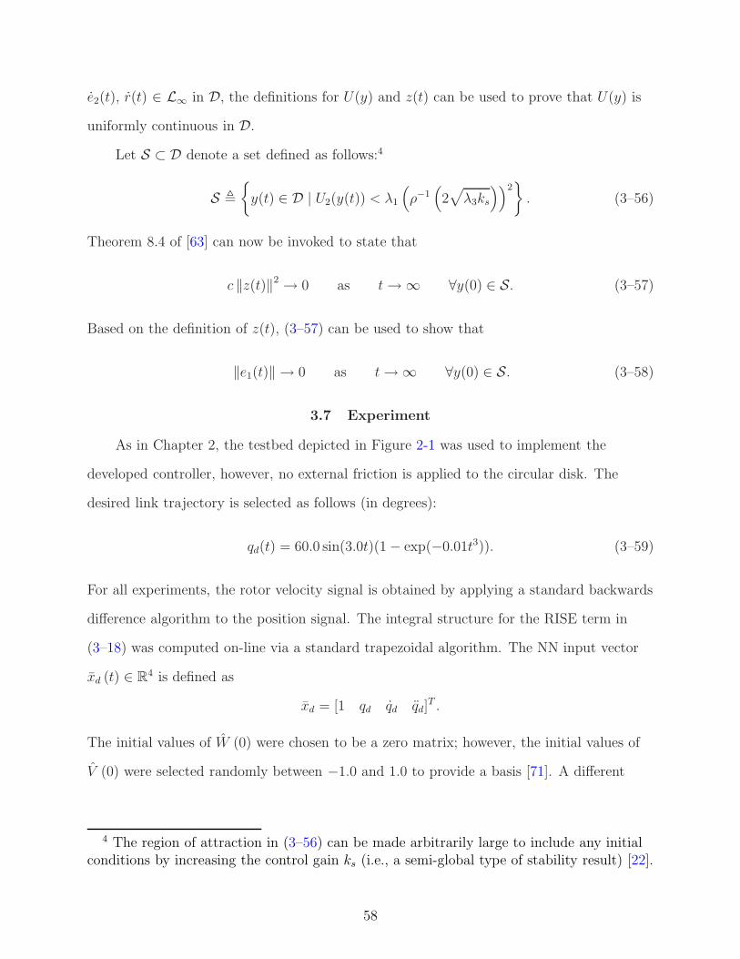
e2(t), r(t) ∈ L∞ in D, the definitions for U(y) and z(t) can be used to prove that U(y) is

uniformly continuous in D.

Let S ⊂ D denote a set defined as follows:4

S ,

y(t) ∈ D | U2(y(t)) < λ1

(

ρ−1(

2√

λ3ks

))2

. (3–56)

Theorem 8.4 of [63] can now be invoked to state that

c ‖z(t)‖2 → 0 as t→ ∞ ∀y(0) ∈ S. (3–57)

Based on the definition of z(t), (3–57) can be used to show that

‖e1(t)‖ → 0 as t→ ∞ ∀y(0) ∈ S. (3–58)

3.7 Experiment

As in Chapter 2, the testbed depicted in Figure 2-1 was used to implement the

developed controller, however, no external friction is applied to the circular disk. The

desired link trajectory is selected as follows (in degrees):

qd(t) = 60.0 sin(3.0t)(1 − exp(−0.01t3)). (3–59)

For all experiments, the rotor velocity signal is obtained by applying a standard backwards

difference algorithm to the position signal. The integral structure for the RISE term in

(3–18) was computed on-line via a standard trapezoidal algorithm. The NN input vector

xd (t) ∈ R4 is defined as

xd = [1 qd qd qd]T .

The initial values of W (0) were chosen to be a zero matrix; however, the initial values of

V (0) were selected randomly between −1.0 and 1.0 to provide a basis [71]. A different

4 The region of attraction in (3–56) can be made arbitrarily large to include any initialconditions by increasing the control gain ks (i.e., a semi-global type of stability result) [22].

58

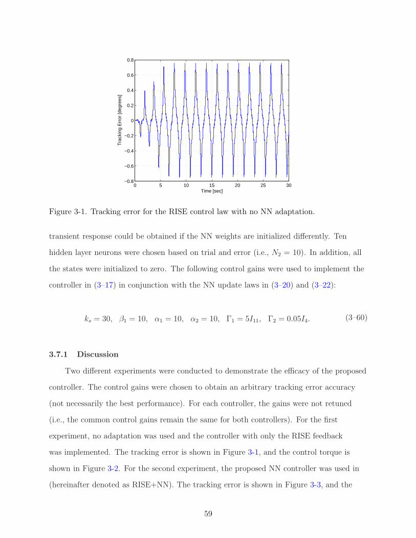
0 5 10 15 20 25 30−0.8

−0.6

−0.4

−0.2

0

0.2

0.4

0.6

0.8

Tra

ckin

g E

rror

[deg

rees

]

Time [sec]

Figure 3-1. Tracking error for the RISE control law with no NN adaptation.

transient response could be obtained if the NN weights are initialized differently. Ten

hidden layer neurons were chosen based on trial and error (i.e., N2 = 10). In addition, all

the states were initialized to zero. The following control gains were used to implement the

controller in (3–17) in conjunction with the NN update laws in (3–20) and (3–22):

ks = 30, β1 = 10, α1 = 10, α2 = 10, Γ1 = 5I11, Γ2 = 0.05I4. (3–60)

3.7.1 Discussion

Two different experiments were conducted to demonstrate the efficacy of the proposed

controller. The control gains were chosen to obtain an arbitrary tracking error accuracy

(not necessarily the best performance). For each controller, the gains were not retuned

(i.e., the common control gains remain the same for both controllers). For the first

experiment, no adaptation was used and the controller with only the RISE feedback

was implemented. The tracking error is shown in Figure 3-1, and the control torque is

shown in Figure 3-2. For the second experiment, the proposed NN controller was used in

(hereinafter denoted as RISE+NN). The tracking error is shown in Figure 3-3, and the

59

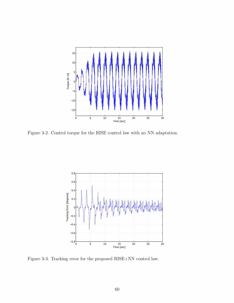
0 5 10 15 20 25 30

−15

−10

−5

0

5

10

15

Tor

que

[N−

m]

Time [sec]

Figure 3-2. Control torque for the RISE control law with no NN adaptation.

0 5 10 15 20 25 30−0.8

−0.6

−0.4

−0.2

0

0.2

0.4

0.6

0.8

Tra

ckin

g E

rror

[deg

rees

]

Time [sec]

Figure 3-3. Tracking error for the proposed RISE+NN control law.

60

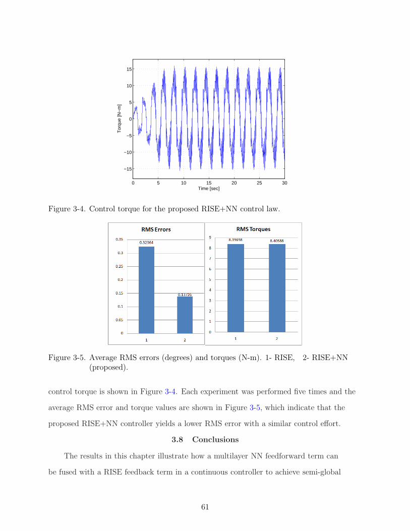
0 5 10 15 20 25 30

−15

−10

−5

0

5

10

15

Tor

que

[N−

m]

Time [sec]

Figure 3-4. Control torque for the proposed RISE+NN control law.

Figure 3-5. Average RMS errors (degrees) and torques (N-m). 1- RISE, 2- RISE+NN(proposed).

control torque is shown in Figure 3-4. Each experiment was performed five times and the

average RMS error and torque values are shown in Figure 3-5, which indicate that the

proposed RISE+NN controller yields a lower RMS error with a similar control effort.

3.8 Conclusions

The results in this chapter illustrate how a multilayer NN feedforward term can

be fused with a RISE feedback term in a continuous controller to achieve semi-global

61

asymptotic tracking. Improved weight tuning laws are presented which guarantee

boundedness of NN weights. To blend the NN and RISE methods, several technical

challenges were addressed through Lyapunov-based techniques. These challenges include

developing adaptive update laws for the NN weight estimates that do not depend on

acceleration, and developing new RISE stability analysis methods and sufficient gain

conditions to accommodate the incorporation of the NN adaptive updates in the RISE

structure. Experimental results are presented that indicate reduced RMS tracking errors

while requiring slightly higher RMS control effort.

62

CHAPTER 4A NEW CLASS OF MODULAR ADAPTIVE CONTROLLERS

4.1 Introduction

The results in this chapter provide the first investigation of the ability to yield

controller/update law modularity using the RISE feedback. First, we consider a general

class of multi-input multi-output (MIMO) dynamic systems with structured (i.e., LP)

and unstructured uncertainties and develop a controller with modularity between

the controller/update law, where a model-based adaptive feedforward term is used

in conjunction with the RISE feedback term [19]. The RISE-based modular adaptive

approach is different than previous work (cf. [40, 41, 43]) in the sense that it does not

rely on nonlinear damping. The use of the RISE method in lieu of nonlinear damping

has several advantages that motivate this investigation including: an asymptotic modular

adaptive tracking result can be obtained for nonlinear systems with non-LP additive

bounded disturbances; the dual objectives of asymptotic tracking and controller/update

law modularity are achieved in a single step unlike the two stage analysis required in some

results (cf., [40, 43]); the development does not require that the adaptive estimates are

a priori bounded; and the development does not require a positive definite estimate of

the inertia matrix or a square integrable prediction error as in [40, 43]. Modularity in the

adaptive feedforward term is made possible by considering a generic form of the adaptive

update law and its corresponding parameter estimate. The general form of the adaptive

update law includes examples such as gradient, least-squares, and etc. This generic form

of the update law is used to develop a new closed-loop error system, and the typical RISE

stability analysis is modified to accommodate the generic update law. New sufficient gain

conditions are derived to prove an asymptotic tracking result.

The class of RISE-based modular adaptive controllers is then extended to include

uncertain dynamic systems that do not satisfy the LP assumption. Neural networks (NNs)

have gained popularity as a feedforward adaptive control method that can compensate

63

for non-LP uncertainty in nonlinear systems. A limiting factor in previous NN-based

feedforward control results is that a residual function approximation error exists that

limits the steady-state performance to a uniformly ultimately bounded result, rather

than an asymptotic result. Some results (cf. [33–36, 72–74]) have been developed to

augment the NN feedforward component with a discontinuous feedback element to achieve

asymptotic tracking. Motivated by the practical limitations of discontinuous feedback,

a multilayer NN-based controller was augmented by RISE feedback in [75] to yield the

first asymptotic tracking result using a continuous controller. However, in most NN-based

controllers, the NN adaptation is governed by a gradient update law to facilitate the

Lyapunov-based stability analysis.

Since multilayer NNs are nonlinear in the weights, a challenge is to derive weight

tuning laws in closed-loop feedback control systems that yield stability as well as bounded

weights. The development in the current chapter illustrates how to extend the class of

modular adaptive controllers for NNs. Specifically, the result allows the NN weight tuning

laws to be determined from a developed generic update law (rather than be restricted to

a gradient update law). We are not aware of any modular multilayer NN-based controller

in literature with modularity in the tuning laws/controller. The NN feedforward structure

adaptively compensates for the non-LP uncertain dynamics. For the tuning laws that

could be used in this result, the NN weights can be initialized randomly, and no off-line

training is required.

The modular adaptive control development for the general class of multi-input

systems is then applied to a class of dynamic systems modeled by the Euler-Lagrange

formulation. The Euler-Lagrange formulation describes the behavior of a large class

of engineering systems (e.g., robot manipulators, satellites, vehicular systems). An

experimental section is included that illustrates that different adaptation laws can be

included with the feedback controller through examples including a gradient update law

and a least squares update law for the LP dynamics case, and a common gradient weight

64

tuning law based on backpropagated error [76] and a simplified tuning law based on the

Hebbian algorithm [77] for the non-LP dynamics case.

While the current result encompasses a large variety of adaptive update laws, an

update law design based on the prediction error is not possible because the formulation of

a prediction error requires the system dynamics to be completely LP. Future efforts can

focus on developing a RISE-based adaptive controller for a completely LP system that

could also use a prediction error/torque filtering approach. Also, one of the shortcomings

of current work is that only a semi-global asymptotic stability is achieved, and further

investigation is needed to achieve a global stability result. Inroads to solve the global

tracking problem are provided in [78] under a set of assumptions.

4.2 Dynamic System

Consider a class of MIMO nonlinear systems of the following form:

x(m) = f(x, x, ..., x(m−1)) +G(x, x, ..., x(m−1))u+ h (t) , (4–1)

where (·)(i) (t) denotes the ith derivative with respect to time, x(i) (t) ∈ Rn, i = 0, ..., m− 1

are the system states, u (t) ∈ Rn is the control input, f (·) ∈ Rn and G (·) ∈ Rn×n are

unknown nonlinear C2 functions, and h (t) ∈ Rn denotes a general nonlinear disturbance

(e.g., unmodeled effects). The outputs of the system are the system states. Throughout

the chapter |·| denotes the absolute value of the scalar argument, ‖·‖ denotes the standard

Euclidean norm for a vector or the induced infinity norm for a matrix, and ‖·‖F denotes

the Frobenius norm of a matrix.

The subsequent development is based on the assumption that all the system states are

measurable. Moreover, the following properties and assumptions will be exploited in the

subsequent development.

Assumption 4-1: G (·) is symmetric positive definite, and satisfies the following

inequality ∀y(t) ∈ Rn:

g ‖y‖2 ≤ yTG−1(·)y ≤ g(x, x, ..., x(m−1)) ‖y‖2 , (4–2)

65

where g ∈ R is a known positive constant, g(x, x, ..., x(m−1)) ∈ R is a known positive

function.

Assumption 4-2: The functions G−1(·) and f(·) are second order differentiable such that

G−1(·), G−1(·), G−1(·), f(·), f(·), f(·) ∈ L∞ if x(i) (t) ∈ L∞, i = 0, 1, ..., m+ 1.

Assumption 4-3: The nonlinear disturbance term and its first two time derivatives (i.e.,

h (t) , h (t) , h (t)) are bounded by known constants.

Assumption 4-4: The unknown nonlinearities G−1(·) and f(·) are linear in terms of

unknown constant system parameters (i.e., LP).

Assumption 4-5: The desired trajectory xd(t) ∈ Rn is assumed to be designed such that

x(i)d (t) ∈ L∞, i = 0, 1, ..., m+ 2.

4.3 Control Objective

The objective is to design a continuous modular adaptive controller which ensures

that the system tracks a desired time-varying trajectory xd(t) despite uncertainties and

bounded disturbances in the dynamic model. To quantify this objective, a tracking error,

denoted by e1(t) ∈ Rn, is defined as

e1 , xd − x. (4–3)

To facilitate a compact presentation of the subsequent control development and stability

analysis, auxiliary error signals denoted by ei (t) ∈ Rn, i = 2, 3, ..., m are defined as

e2 , e1 + α1e1

e3 , e2 + α2e2 + e1

e4 , e3 + α3e3 + e2

...

ei , ei−1 + αi−1ei−1 + ei−2 (4–4)

...

66

em , em−1 + αm−1em−1 + em−2,

where αi ∈ R, i = 1, 2, ..., m − 1 denote constant positive control gains. The error signals

ei (t) , i = 2, 3, ..., m can be expressed in terms of e1 (t) and its time derivatives as

ei =i−1∑

j=0

ai,je(j)1 , (4–5)

where the constant coefficients ai,j ∈ R can be evaluated by substituting (4–5) in (4–4),

and comparing coefficients [79]. A filtered tracking error [57], denoted by r(t) ∈ Rn, is also

defined as

r , em + αmem, (4–6)

where αm ∈ R is a positive, constant control gain. The filtered tracking error r(t) is not

measurable since the expression in (4–6) depends on x(m)(t).

4.4 Control Development

The open-loop tracking error system is developed by premultiplying (4–6) by

G−1(

x, x, ..., x(m−1))

and utilizing the expressions in (4–1), (4–4), (4–5) as

G−1r = Ydθ + S −G−1d h− u (4–7)

where the fact that am,m−1 = 1, was used. In (4–7), Ydθ ∈ Rn is defined as

Ydθ , G−1d x

(m)d −G−1

d fd, (4–8)

where Yd(xd, xd, ..., x(m)d ) ∈ Rn×p is a desired regression matrix, and θ ∈ Rp contains the

constant unknown system parameters. In (4–8), the functions G−1d (xd, xd, ..., x

(m−1)d ) ∈

Rn×n, fd(xd, xd, ..., x(m−1)d ) ∈ Rn are defined as

G−1d , G−1(xd, xd, ..., x

(m−1)d ) (4–9)

fd , f(xd, xd, ..., x(m−1)d ).

67

Also in (4–7), the auxiliary function S(

x, x, ..., x(m−1), t)

∈ Rn is defined as

S , G−1

(

m−2∑

j=0

am,je(j+1)1 + αmem

)

+G−1x(m)d −G−1

d x(m)d −G−1f +G−1

d fd −G−1h+G−1d h.

(4–10)

Based on the open-loop error system in (4–7), the control input is composed of an

adaptive feedforward term plus the RISE feedback term as

u , Ydθ + µ. (4–11)

In (4–11), µ(t) ∈ Rn denotes the RISE feedback term defined as [19, 22]

µ (t) , (ks + 1)em(t) − (ks + 1)em(0) +

∫ t

0

[(ks + 1)αmem(σ) + β1sgn(em(σ))]dσ, (4–12)

where ks, β1 ∈ R are positive constant control gains, and αm ∈ R was introduced in (4–6).

In (4–11), θ (t) ∈ Rp denotes a subsequently designed parameter estimate vector. The

closed-loop tracking error system is developed by substituting (4–11) into (4–7) as

G−1r = Yd

(

θ − θ)

+ S −G−1d h− µ. (4–13)

To facilitate the subsequent modular adaptive control development and stability analysis,

the time derivative of (4–13) is expressed as

G−1r = −1

2G−1r + N(t) +NB (t) − (ks + 1)r − β1sgn(em) − em, (4–14)

where the fact that the time derivative of (4–12) is given as

µ(t) = (ks + 1)r + β1sgn(em) (4–15)

was utilized. In (4–14), the unmeasurable/unknown auxiliary terms N(e1, e2, ..., em, r, t),

NB (t) ∈ Rn are defined as

N(t) , −1

2G−1r + S + em + N0 (4–16)

68

NB (t) , NB1 (t) +NB2 (t) , (4–17)

where NB1 (t) ∈ Rn is given by

NB1 , Ydθ − G−1d h−G−1

d h, (4–18)

and the sum of the auxiliary terms N0(t), NB2 (t) ∈ Rn is given by

NB2 (t) + N0 = −Ydθ − Yd

·

θ. (4–19)

Specific definitions for N0(t), NB2 (t) are provided subsequently based on the definition

of the adaptive update law for θ (t). The structure of (4–14) and the introduction of the

auxiliary terms in (4–16)-(4–19) is motivated by the desire to segregate terms that can

be upper bounded by state-dependent terms and terms that can be upper bounded by

constants. Specifically, depending on how the adaptive update law is designed, analysis is

provided in the next section to upper bound N(t) by state-dependent terms and NB (t) by

a constant. The need to further segregate NB (t) is that some terms in NB (t) have time

derivatives that are upper bounded by a constant, while other terms have time-derivatives

that are upper-bounded by state dependent terms. The segregation of these terms based

on the structure of the adaptive update law (see (4–19)) is key for the development of a

stability analysis for the modular RISE-based adaptive update law/controller.

4.5 Modular Adaptive Update Law Development

A key difference between the traditional modular adaptive controllers that use

nonlinear damping (cf., [1, 41, 63]) and the current RISE-based approach is that the

RISE-based method does not exploit the ISS property with respect to the parameter

estimation error. The current approach does not rely on nonlinear damping, but instead

uses the ability of the RISE technique to compensate for smooth bounded disturbances.

In general, previous nonlinear damping-based modular adaptive controllers first prove an

ISS stability result provided the adaptive update law yields bounded parameter estimates

(e.g., θ (t) ∈ L∞ via a projection algorithm), and then use additional analysis along with

69

assumptions (PD estimate of the inertia matrix, square integrable prediction error, etc.)

to conclude asymptotic convergence. In contrast, since the RISE-based modular adaptive

control approach in this chapter does not exploit an ISS analysis, the assumptions

regarding the parameter estimate are modified. The following development requires some

general bounds on the structure of the adaptive update law·

θ (t) and the corresponding

parameter estimate θ (t) to segregate the components of the auxiliary terms introduced

in (4–16)-(4–19). Specifically, instead of assuming that θ (t) ∈ L∞, the subsequent

development is based on the less restrictive assumption that the parameter estimate θ (t)

can be described as

θ (t) = f1 (t) + Φ(x, x, ..., x(m−1), e1, e2, ..., em, t). (4–20)

In (4–20), f1 (t) ∈ Rp is a known function such that

‖f1 (t)‖ ≤ γ1 (4–21)

∥

∥

∥f1 (t)

∥

∥

∥≤ γ2 +

m∑

i=1

γi+2 ‖ei‖ + γm+3 ‖r‖ ,

where γi ∈ R, i = 1, 2, ..., m+ 3 are known non-negative constants (i.e., the constants can

be set to zero for different update laws), and Φ(

x, x, ..., x(m−1), e1, e2, ..., em, t)

∈ Rp is a

known function that satisfies the following bound:

‖Φ (t)‖ ≤ ρ1 (‖e‖) ‖e‖ , (4–22)

where the bounding function ρ1(·) ∈ R is a positive, globally invertible, nondecreasing

function, and e(t) ∈ Rnm is defined as

e(t) ,[

eT1 eT

2 ... eTm

]T. (4–23)

70

The estimate in (4–20) is assumed to be generated according to an update law of the

following general form

·

θ (t) = g1 (t) + Ω(x, x, ..., x(m−1), e1, e2, ..., em, r, t). (4–24)

In (4–24), g1 (t) ∈ Rp is a known function such that

‖g1 (t)‖ ≤ δ1 (4–25)

‖g1 (t)‖ ≤ δ2 +m∑

i=1

δi+2 ‖ei‖ + δm+3 ‖r‖ ,

where δi ∈ R, i = 1, 2, ..., m+ 3 are known non-negative constants, and Ω(x, x, ..., x(m−1),

e1, e2, ..., em, r, t) ∈ Rp satisfies the following bound:

‖Ω (t)‖ ≤ ρ2 (‖z‖) ‖z‖ , (4–26)

where the bounding function ρ2(·) ∈ R is a positive, globally invertible, nondecreasing

function, and z(t) ∈ Rn(m+1) is defined as

z(t) ,[

eT1 eT

2 ... eTm rT

]T. (4–27)

Remark 4.1. The update law in (4–24) depends on the unmeasurable signal r(t). But it

is assumed that the update law in (4–24) is of the form which upon integration yields an

estimate θ (t) that is independent of r(t). Thus the controller needs only the measurable

signals for implementation.

The structure of the adaptive estimate and the adaptive update law is flexible in the

sense that any of the terms in (4–20) and (4–24) can be removed for any specific update

law and estimate. For example if all the error-dependent terms in (4–20) are removed,

then the condition on θ (t) is the same as in the standard nonlinear damping-based

modular adaptive methods (i.e., θ (t) ∈ L∞). In this sense, the ISS property with

respect to the parameter estimation error is automatically proven by considering this

special case of θ (t). The results in this chapter are not proven for estimates or update

71

laws with additional terms that are not included in the generic structure in (4–20) and

(4–24). For example, a standard gradient-based update law is of the form (4–24), but the

corresponding estimate (obtained via integration by parts) is not of the form (4–20) due to

the presence of some terms that are bounded by the integral of the error instead of being

bounded by the error. However, the same gradient-based update law and its corresponding

estimate can be used in (4–11) if a smooth projection algorithm is used that keeps the

estimates bounded. As shown in [19], the standard gradient-based update law can be

used in (4–11) without a projection algorithm, yet including this structure in the modular

adaptive analysis is problematic because the integral of the error could be unbounded

(so this update law could not be used in nonlinear damping-based modular adaptive laws

without a projection either). Since the goal in this chapter is to develop a modular update

law, a specific update law cannot be used to inject terms in the stability analysis to cancel

the terms containing the parameter mismatch error. Instead, the terms containing the

parameter mismatch error are segregated depending on whether they are state-dependent

or bounded by a constant (see (4–19)).

Based on the development given in (4–20)-(4–25), the terms N0(t) and NB2 (t)

introduced in (4–16)-(4–19) are defined as

N0(t) , −YdΦ − YdΩ (4–28)

NB2 (t) , −Ydf1 − Ydg1. (4–29)

In a similar manner as in Lemma 1 of the Appendix, by applying the Mean Value

Theorem along with the inequalities in (4–22) and (4–26) yields an upper bound for

the expression in (4–16) as∥

∥

∥N(t)

∥

∥

∥≤ ρ (‖z‖) ‖z‖ , (4–30)

where the bounding function ρ(·) ∈ R is a positive, globally invertible, nondecreasing

function, and z(t) ∈ Rn(m+1) is defined in (4–27). The following inequalities are

developed based on the expressions in (4–17), (4–18), (4–29), their time derivatives,

72

and the inequalities in (4–21) and (4–25):

‖NB(t)‖ ≤ ζ1

∥

∥

∥NB1(t)

∥

∥

∥≤ ζ2 (4–31)

∥

∥

∥NB2(t)

∥

∥

∥≤ ζ3 +

m∑

i=1

ζi+3 ‖ei‖ + ζm+4 ‖r‖ ,

where ζi ∈ R, i = 1, 2, ..., m+ 4 are known positive constants.

4.6 Stability Analysis

Theorem 4-1: The controller given in (4–11), (4–12), (4–20), and (4–24) ensures

that all system signals are bounded under closed-loop operation and that the position

tracking error is regulated in the sense that

‖e1(t)‖ → 0 as t→ ∞

provided the control gain ks introduced in (4–12) is selected sufficiently large (see the

subsequent proof), αi, i = 1, 2, ..., m are selected according to the following conditions

αi >1

2βi+1, i = 1, 2, ..., m− 2 αm−1 >

1

2βm +

1

2(4–32)

αm > βm+1 +1

2βm+2 +

1

2

m−1∑

i=1

βi+1 +1

2,

and βi, i = 1, 2, ..., m+ 2 are selected according to the following sufficient conditions:

β1 > ζ1 +1

αm

ζ2 +1

αm

ζ3 (4–33)

βi+1 > ζi+3, i = 1, 2, ..., m+ 1,

where β1 was introduced in (4–12), and β2, ..., βm+2 are introduced in (4–36).

Proof: Let D ⊂ Rn(m+1)+1 be a domain containing y(t) = 0, where y(t) ∈ Rn(m+1)+1 is

defined as

y(t) , [zT (t)√

P (t)]T . (4–34)

73

In (4–34), the auxiliary function P (t) ∈ R is defined as

P (t) , β1

n∑

i=1

|emi(0)| − em(0)TNB(0) −

∫ t

0

L(τ)dτ, (4–35)

where emi (0) denotes the ith element of the vector em (0), and the auxiliary function

L(t) ∈ R is defined as

L(t) , rT (NB(t) − β1sgn(em)) −m∑

i=1

βi+1 ‖ei(t)‖ ‖em(t)‖ − βm+2 ‖em(t)‖ ‖r(t)‖ , (4–36)

where βi ∈ R, i = 2, 3, ..., m + 2 are positive constants chosen according to the sufficient

conditions in (4–33). Provided the sufficient conditions introduced in (4–33) are satisfied,

the following inequality is obtained1 :

∫ t

0

L(τ)dτ ≤ β1

n∑

i=1

|emi(0)| − em(0)TNB(0). (4–37)

Hence, (4–37) indicates that P (t) ≥ 0.

Let VL(y, t) : D × [0,∞) → R be a continuously differentiable, positive definite

function defined as

VL(y, t) ,1

2

m∑

i=1

eTi ei +

1

2rTG−1r + P, (4–38)

which satisfies the following inequalities:

U1(y) ≤ VL(y, t) ≤ U2(y) (4–39)

provided the sufficient conditions introduced in (4–32)-(4–33) are satisfied. The Rayleigh-Ritz

theorem was used to develop the inequalities in (4–39), where the continuous positive

definite functions U1(y),U2(y) ∈ R are defined as U1(y) , λ1 ‖y‖2 and U2(y) ,

λ2(x, x, ..., x(m−1)) ‖y‖2, where λ1, λ2(x, x, ..., x

(m−1)) ∈ R are defined as

λ1 ,1

2min

1, g

λ2(x, x, ..., x(m−1)) , max

1

2g(x, x, ..., x(m−1)), 1, (4–40)

1 Details of the bound in (4–37) are provided in the Lemma 1 of the Appendix.

74

where g, g(x, x, ..., x(m−1)) are introduced in (4–2). After taking the time derivative of

(4–38), V (y, t) is expressed as

VL(y, t) = rTG−1r +1

2rT G−1r +

m∑

i=1

eTi ei + P .

The derivative P (t) ∈ R is given by

P (t) = −L(t) = −rT (NB(t) − β1sgn(em)) +m∑

i=1

βi+1 ‖ei(t)‖ ‖em(t)‖ + βm+2 ‖em(t)‖ ‖r(t)‖ .

(4–41)

After utilizing (4–4), (4–6), (4–14), (4–15), and (4–41), V (y, t) is expressed as

VL(y, t) =1

2rT G−1r −

m∑

i=1

αieTi ei + eT

m−1em −1

2rT G−1r

+ rT N + rTNB − rT r − ksrT r − β1r

T sgn(em)

− rT (NB − β1sgn(em)) +m∑

i=1

βi+1 ‖ei‖ ‖em‖ + βm+2 ‖em‖ ‖r‖ .

After canceling similar terms, V (y, t) is simplified as

VL(y, t) = −

m∑

i=1

αieTi ei + eT

m−1em − rT r − ksrT r + rT N

+m∑

i=1

βi+1 ‖ei‖ ‖em‖ + βm+2 ‖em‖ ‖r‖ .

Based on the fact that aT b ≤ 12(‖a‖2 + ‖b‖2) for some a, b ∈ Rn, VL(y, t) is upper bounded

using the squares of the components of z(t) as

VL(y, t) ≤ −m−2∑

i=1

(αi −1

2βi+1) ‖ei‖

2 − (αm−1 −1

2βm −

1

2) ‖em−1‖

2

− (αm − βm+1 −1

2βm+2 −

1

2

m−1∑

i=1

βi+1 −1

2) ‖em‖

2 − ‖r‖2 (4–42)

− (ks −1

2βm+2) ‖r‖

2 + rT N.

75

By using (4–30), the expression in (4–42) is rewritten as

VL(y, t) ≤ −λ3 ‖z‖2 −

[

(ks −βm+2

2) ‖r‖2 − ρ(‖z‖) ‖r‖ ‖z‖

]

, (4–43)

where

λ3 , minα1 −1

2β2, α2 −

1

2β3, ..., αm−2 −

1

2βm−1,

αm−1 −1

2βm −

1

2, αm − βm+1 −

1

2βm+2 −

1

2

m−1∑

i=1

βi+1 −1

2, 1.

After completing the squares for the terms inside the brackets in (4–43), the following

expression can be obtained, provided the sufficient gain conditions in (4–32) and (4–33)

are satisfied:

VL(y, t) ≤ −λ3 ‖z‖2 +

ρ2(‖z‖) ‖z‖2

4(

ks −βm+2

2

) . (4–44)

The expression in (4–44) can be further upper bounded by a continuous, positive

semi-definite function

VL(y, t) ≤ −U(y) = −c ‖z‖2 ∀y ∈ D (4–45)

for some positive constant c ∈ R, where

D ,

y ∈ Rn(m+1)+1 | ‖y‖ ≤ ρ−1

(

2

√

λ3

(

ks −βm+2

2

)

)

.

Larger values of k will expand the size of the domain D. The inequalities in (4–39) and

(4–45) indicate that VL(y, t) ∈ L∞ in D; hence, ei(t) ∈ L∞, and r(t) ∈ L∞ in D. Given

that ei(t) ∈ L∞, and r(t) ∈ L∞ in D, then ei(t) ∈ L∞ in D from (4–4) and (4–6). Since

ei(t) ∈ L∞, and r(t) ∈ L∞ in D, the assumption that x(i)d (t) exist and are bounded and

(4–3)-(4–6) indicate that x(i)(t) ∈ L∞ in D. Since x(i)(t) ∈ L∞ in D, (4–20)-(4–25) indicate

that θ(t),·

θ(t) ∈ L∞ in D, and G−1(·) and f(·) ∈ L∞ in D from Property 2. Thus, from

(4–1) and Property 3, we can show that u(t) ∈ L∞ in D. Given that r(t) ∈ L∞ in D,

(4–15) indicates that µ(t) ∈ L∞ in D. Since x(i)(t) ∈ L∞ in D, then G−1(·) and f(·) ∈ L∞

76

in D based on Property 2; hence, (4–14) indicates that r(t) ∈ L∞ in D. Since ei(t) ∈ L∞

and r(t) ∈ L∞ in D, then U(y) is uniformly continuous in D based on the definitions for

U(y) and z(t).

Let S ⊂ D denote a set defined as

S ,

y(t) ∈ D | U2(y(t)) < λ1

(

ρ−1

(

2

√

λ3

(

ks −βm+2

2

)

))2

. (4–46)

The region of attraction in (4–46) is arbitrarily large and can include any initial condition

by increasing the control gain ks (i.e., a semi-global stability result). By invoking Theorem

8.4 of [63]

c ‖z(t)‖2 → 0 as t→ ∞ ∀y(0) ∈ S. (4–47)

Based on the definition of z(t), (4–47) indicates that

‖e1(t)‖ → 0 as t→ ∞ ∀y(0) ∈ S. (4–48)

4.7 Neural Network Extension to Non-LP Systems

The class of RISE-based modular adaptive controllers developed in the preceding

sections are extended to include uncertain dynamic systems that do not satisfy the LP

assumption (i.e., Assumption 4-4 is not satisfied). NN-based estimation methods are well

suited for control systems where the dynamic model contains unstructured nonlinear

disturbances as in (4–1). The main feature that empowers NN-based controllers is the

universal approximation property as described in Section 3.4 of Chapter 3.

4.7.1 RISE Feedback Control Development

The modular control development and stability analysis is provided to illustrate

how the aforementioned textbook (e.g., [15]) NN feedforward estimation strategy can be

fused with a RISE feedback control method as a means to achieve asymptotic stability for

general class of MIMO systems described by (4–1) while using generic NN weight update

laws. The open-loop and closed-loop tracking error is developed for the combined control

system.

77

Similar to (4–7), the open-loop tracking error system is developed by premultiplying

(4–6) by G−1 and utilizing the expressions in (4–1) and (4–4) to obtain:

G−1r = fNN + S −G−1d h− u, (4–49)

where the auxiliary function fNN (xd, xd, ..., x(m)d ) ∈ R

n is defined as

fNN , G−1d x

(m)d −G−1

d fd, (4–50)

where G−1d (xd, xd, ..., x

(m−1)d ) ∈ Rn×n and fd(xd, xd, ..., x

(m−1)d ) ∈ Rn are defined in (4–9). In

(4–49), the auxiliary function S(

x, x, ..., x(m−1), t)

∈ Rn is defined similar to (4–10). The

expression in (4–50) can be represented by a three-layer NN as

fNN = W Tσ(

V T xd

)

+ ε (xd) . (4–51)

In (4–51), the input xd(t) ∈ R(m+1)n+1 is defined as xd(t) , [1 xTd (t) xT

d (t) ... x(m)Td (t)]T

so that N1 = (m+ 1)n where N1 was introduced in (3–4). Based on the assumption

that the desired trajectory is bounded, the inequalities in (3–16) hold. Based on the

open-loop error system in (4–49), the control torque input is composed of a three-layer NN

feedforward term plus the RISE feedback term as

u , fNN + µ (4–52)

where the RISE feedback term µ ∈ Rn is defined in (4–12), and the feedforward NN

component denoted by fNN(t) ∈ Rn, is defined as

fNN , W Tσ(V T xd). (4–53)

78

4.7.2 Modular Tuning Law Development

The estimates for the NN weights in (4–53) are generated on-line (there is no off-line

learning phase) using a smooth projection algorithm as

·

W , proj (%1) =

%1 if vec(W ) ∈ int(ΛW )

%1 if vec(W ) ∈ ∂(ΛW ) and vec (%1)T vec(W )⊥ ≤ 0

P tMr (%1) if vec(W ) ∈ ∂(ΛW ) and vec (%1)

T vec(W )⊥ > 0

(4–54)

·

V , proj (%2) =

%2 if vec(V ) ∈ int(ΛV )

%2 if vec(V ) ∈ ∂(ΛV ) and vec (%2)T vec(V )⊥ ≤ 0

P tMr (%2) if vec(V ) ∈ ∂(ΛV ) and vec (%2)

T vec(V )⊥ > 0,

(4–55)

where proj (·) is the projection operator and

vec(W (0)) ∈ int (ΛW ) , vec(V (0)) ∈ int (ΛV ) .

In (4–54) and (4–55), the auxiliary terms %1(t) ∈ R(N2+1)×n and %2(t) ∈ R(N1+1)×N2 denote

adaptation rules of the following general form:

proj (%1) = w1 (t) + ΞW (x, x, ..., x(m−1), e1, e2, ..., em, r, t) (4–56)

proj (%2) = v1 (t) + ΞV (x, x, ..., x(m−1), e1, e2, ..., em, r, t).

In (4–56), w1 (t) ∈ R(N2+1)×n and v1 (t) ∈ R(N1+1)×N2 are known functions such that

‖w1 (t)‖ ≤ γ1 (4–57)

‖w1 (t)‖ ≤ γ2 +m∑

i=1

γi+2 ‖ei‖ + γm+3 ‖r‖

‖v1 (t)‖ ≤ δ1 (4–58)

‖v1 (t)‖ ≤ δ2 +

m∑

i=1

δi+2 ‖ei‖ + δm+3 ‖r‖ ,

79

and ΞW ∈ R(N2+1)×n and ΞV ∈ R

(N1+1)×N2 satisfy the following bounds:

‖ΞW (t)‖ ≤m∑

i=1

γi+m+3 ‖ei‖ + γ2m+4 ‖r‖ (4–59)

‖ΞV (t)‖ ≤

m∑

i=1

δi+m+3 ‖ei‖ + δ2m+4 ‖r‖ ,

where γi, δi ∈ R, i = 1, 2, ..., 2m + 4 are known non-negative constants (i.e., the

constants can be set to zero for different update laws). In (4–54) and (4–55), P tMr (A) =

devec (P tr (vec (A))) for a matrix A, where the operation devec (·) is the reverse of vec (·).

The use of the projection algorithm in (4–54) and (4–55) is to ensure that W (t) and

V (t) remain bounded inside the convex regions defined in (3–9) and (3–11). This fact

will be exploited in the subsequent stability analysis. Thus, unlike the general form for

parameter estimate θ (t) in (4–20) for the LP case, the NN weight estimates are bounded

by constants. The NN weight adaptation laws are restrictive compared to the adaptive

laws for the parameter estimates in the LP case. This is because the first layer weight

estimates V (t) are embedded inside the nonlinear activation function σ (·) (i.e., σ(V T xd)).

Typically the NN activation functions are bounded over the entire domain; however, their

time derivatives depend on the adaptation law·

V (t), which could be state-dependent.

Similar to the LP case, it is assumed that only the NN adaptation rules depend on the

unmeasurable signal r (t) but the corresponding weight estimate obtained after integration

is independent of r (t).

The closed-loop tracking error system can be developed by substituting (4–52) into

(4–49) as

G−1r = fNN − fNN + S −G−1d h− µ. (4–60)

To facilitate the subsequent stability analysis, the time derivative of (4–60) is determined

as

G−1r = −G−1r + fNN −·

fNN + S − G−1d h−G−1

d h− µ. (4–61)

80

Using (4–51), (4–53), the closed-loop error system in (4–61) can be expressed as

G−1r = −G−1r +W Tσ′(

V T xd

)

V T·

xd −·

W Tσ(V T xd) (4–62)

− W Tσ′

(V T xd)(·

V T xd + V T·

xd) + ε+ S − G−1d h−G−1

d h− µ,

where σ′

(V T x) ≡ dσ(

V T x)

/d(

V T x)

|V T x=V T x. After adding and subtracting the term

W T σ′

V T·

xd + W T σ′

V T·

xd to (4–62), the following expression can be obtained:

G−1r = −G−1r + W T σ′

V T·

xd + W T σ′

V T·

xd +W Tσ′

V T·

xd −W T σ′

V T·

xd (4–63)

− W T σ′

V T·

xd −·

W T σ − W T σ′

·

V T xd + ε+ S − G−1d h−G−1

d h− µ,

where the notations σ and σ are introduced in (3–6). Substituting the NN weight

adaptation laws in (4–54), (4–55) in (4–63) yields

G−1r = −1

2G−1r + N +NB − em − (ks + 1)r − β1sgn(em), (4–64)

where (4–15) was utilized, and the unmeasurable auxiliary terms N(e1, e2, ..., em, r, t),

NB(W , V , xd,·

xd, t) ∈ Rn are defined as

N , −1

2G−1r − ΞT

W σ − W T σ′

ΞTV xd + S + em (4–65)

NB , NB1 +NB2 . (4–66)

In (4–66), NB1(xd,·

xd, t), NB2(W , V , xd,·

xd, t) ∈ Rn are given by

NB1 = W Tσ′

V T·

xd + ε− G−1d h−G−1

d h (4–67)

NB2 = W T σ′

V T·

xd + W T σ′

V T·

xd − wT1 σ − W T σ

′

vT1 xd (4–68)

In a similar manner as before, application of the Mean Value Theorem will yield an

upper bound for N (t) as in (4–30). The following inequalities are developed based on

Assumptions 4-2 and 4-3, (3–7), (3–8), (3–16), (4–56)-(4–59), and (4–66)-(4–68):

‖NB‖ ≤ ζ1

∥

∥

∥NB1

∥

∥

∥≤ ζ2 (4–69)

81

∥

∥

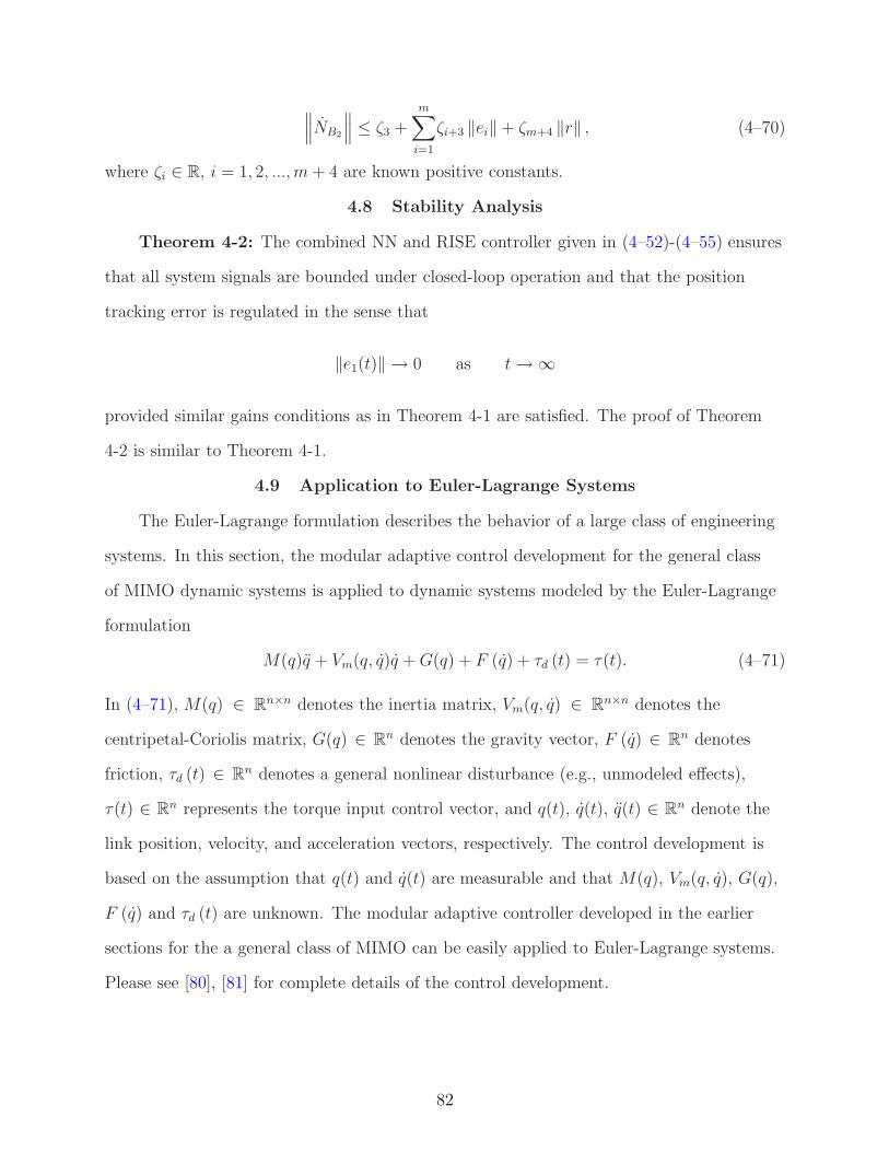
∥NB2

∥

∥

∥≤ ζ3 +

m∑

i=1

ζi+3 ‖ei‖ + ζm+4 ‖r‖ , (4–70)

where ζi ∈ R, i = 1, 2, ..., m+ 4 are known positive constants.

4.8 Stability Analysis

Theorem 4-2: The combined NN and RISE controller given in (4–52)-(4–55) ensures

that all system signals are bounded under closed-loop operation and that the position

tracking error is regulated in the sense that

‖e1(t)‖ → 0 as t→ ∞

provided similar gains conditions as in Theorem 4-1 are satisfied. The proof of Theorem

4-2 is similar to Theorem 4-1.

4.9 Application to Euler-Lagrange Systems

The Euler-Lagrange formulation describes the behavior of a large class of engineering

systems. In this section, the modular adaptive control development for the general class

of MIMO dynamic systems is applied to dynamic systems modeled by the Euler-Lagrange

formulation

M(q)q + Vm(q, q)q +G(q) + F (q) + τd (t) = τ(t). (4–71)

In (4–71), M(q) ∈ Rn×n denotes the inertia matrix, Vm(q, q) ∈ Rn×n denotes the

centripetal-Coriolis matrix, G(q) ∈ Rn denotes the gravity vector, F (q) ∈ R

n denotes

friction, τd (t) ∈ Rn denotes a general nonlinear disturbance (e.g., unmodeled effects),

τ(t) ∈ Rn represents the torque input control vector, and q(t), q(t), q(t) ∈ Rn denote the

link position, velocity, and acceleration vectors, respectively. The control development is

based on the assumption that q(t) and q(t) are measurable and that M(q), Vm(q, q), G(q),

F (q) and τd (t) are unknown. The modular adaptive controller developed in the earlier

sections for the a general class of MIMO can be easily applied to Euler-Lagrange systems.

Please see [80], [81] for complete details of the control development.

82

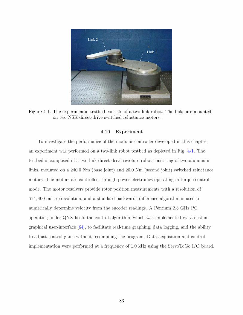
Figure 4-1. The experimental testbed consists of a two-link robot. The links are mountedon two NSK direct-drive switched reluctance motors.

4.10 Experiment

To investigate the performance of the modular controller developed in this chapter,

an experiment was performed on a two-link robot testbed as depicted in Fig. 4-1. The

testbed is composed of a two-link direct drive revolute robot consisting of two aluminum

links, mounted on a 240.0 Nm (base joint) and 20.0 Nm (second joint) switched reluctance

motors. The motors are controlled through power electronics operating in torque control

mode. The motor resolvers provide rotor position measurements with a resolution of

614, 400 pulses/revolution, and a standard backwards difference algorithm is used to

numerically determine velocity from the encoder readings. A Pentium 2.8 GHz PC

operating under QNX hosts the control algorithm, which was implemented via a custom

graphical user-interface [64], to facilitate real-time graphing, data logging, and the ability

to adjust control gains without recompiling the program. Data acquisition and control

implementation were performed at a frequency of 1.0 kHz using the ServoToGo I/O board.

83

The dynamics for the testbed are

τ1

τ2

=

p1 + 2p3c2 p2 + p3c2

p2 + p3c2 p2

q1

q2

+

−p3s2q2 −p3s2 (q1 + q2)

p3s2q2 0

q1

q2

(4–72)

+ f (q) +

τd1

τd2

,

where the nonlinear friction term is assumed to be modeled as [19, 26]

f (q) =

γ1 (tanh (γ2q1) − tanh (γ3q1))

γ1 (tanh (γ2q2) − tanh (γ3q2))

+

γ4 tanh (γ5q1) + γ6q1

γ4 tanh (γ5q2) + γ6q2

. (4–73)

In (4–72) and (4–73), p1, p2, p3, γi ∈ R, (i = 1, 2, ..., 6) are unknown positive constant

parameters, c2 denotes cos(q2), s2 denotes sin(q2), and τd1 , τd2 ∈ R denote general

nonlinear disturbances (e.g., unmodeled effects). Part of the dynamics in (4–72) and

(4–73) is linear in the following parameters:

θ = [p1 p2 p3 γ1 γ4 γ6]T .

The parameters γ2, γ3, γ5 are embedded inside the nonlinear hyperbolic tangent

functions and hence cannot be linearly parameterized. Since these parameters cannot

be compensated for by an adaptive algorithm, best-guess estimates γ2 = 50, γ3 = 1,

γ5 = 50 are used. The values for γ2, γ3, γ5 are based on our previous experiments

concerned with friction identification. Significant errors in these static estimates could

degrade the performance of the system. An advantage of using the NN-based controller

developed in non-LP extension section is that the NN can compensate for the non-LP

dynamics. Specifically, for the NN-based controllers tested in this section, the NN is used

to estimate the friction model, and the best guess values for γ2, γ3, γ5 are not required.

The control objective is to track the desired time-varying trajectory by using the proposed

84

modular adaptive control law. Two different update laws were chosen for both the LP

and non-LP cases. To achieve this control objective, the control gains α1, α2, ks, and β1,

defined as scalars in (4–4), (4–6), and (4–12), were implemented (with non-consequential

implications to the stability result) as diagonal gain matrices. Specifically, the control

gains for both adaptive update laws for both the LP and non-LP cases were selected as

α1 = diag 70, 70 α2 = diag 25, 25

β1 = diag 10, 0.1 ks = diag 100, 20 .

(4–74)

4.10.1 Modular Adaptive Update Law

The desired trajectories for this experiment were chosen as

qd1 = −qd2 = 60 sin(2.0t)(

1 − exp(

−0.01t3))

. (4–75)

To test the modularity of the controller, two separate adaptive update laws were tested

including a standard gradient update law defined as

·

θ = proj(

ΓY Td r)

,

where Γ ∈ R6×6 is a diagonal positive-definite gain matrix, and a least squares update law

defined as·

θ = proj(

PY Td r)

, P = −PY Td YdP

where P (t) ∈ R6×6 is a time-varying symmetric matrix. The parameter estimates were all

initialized to zero. In practice, the adaptive estimates would be initialized to a best-guess

estimate of the values. Initializing the estimates to zero was done to test a scenario of no

parameter knowledge. For the gradient and least squares update laws the adaptation gains

and the initial value of P (t) were selected as

Γ = P (0) = diag ([0.15, 0.01, 0.01, 0.01, 0.01, 0.2]) . (4–76)

85

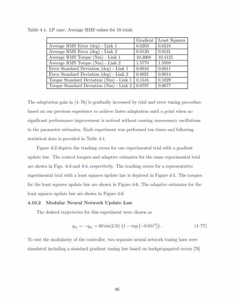
Table 4-1. LP case: Average RMS values for 10 trials

Gradient Least SquaresAverage RMS Error (deg) - Link 1 0.0203 0.0218Average RMS Error (deg) - Link 2 0.0120 0.0131Average RMS Torque (Nm) - Link 1 10.3068 10.4125Average RMS Torque (Nm) - Link 2 1.5770 1.5959Error Standard Deviation (deg) - Link 1 0.0016 0.0011Error Standard Deviation (deg) - Link 2 0.0021 0.0014Torque Standard Deviation (Nm) - Link 1 0.1545 0.1029Torque Standard Deviation (Nm) - Link 2 0.0797 0.0677

The adaptation gain in (4–76) is gradually increased by trial and error tuning procedure

based on our previous experience to achieve faster adaptation until a point when no

significant performance improvement is noticed without causing unnecessary oscillations

in the parameter estimates. Each experiment was performed ten times and following

statistical data is provided in Table 4-1.

Figure 4-2 depicts the tracking errors for one experimental trial with a gradient

update law. The control torques and adaptive estimates for the same experimental trial

are shown in Figs. 4-3 and 4-4, respectively. The tracking errors for a representative

experimental trial with a least squares update law is depicted in Figure 4-5. The torques

for the least squares update law are shown in Figure 4-6. The adaptive estimates for the

least squares update law are shown in Figure 4-6.

4.10.2 Modular Neural Network Update Law

The desired trajectories for this experiment were chosen as

qd1 = −qd2 = 60 sin(2.5t)(

1 − exp(

−0.01t3))

. (4–77)

To test the modularity of the controller, two separate neural network tuning laws were

simulated including a standard gradient tuning law based on backpropagated errors [76]

86

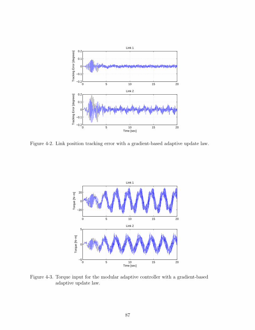
0 5 10 15 20−0.2

−0.1

0

0.1

0.2

Tra

ckin

g E

rror

[deg

rees

]

Link 1

0 5 10 15 20−0.2

−0.1

0

0.1

0.2

Time [sec]

Tra

ckin

g E

rror

[deg

rees

]

Link 2

Figure 4-2. Link position tracking error with a gradient-based adaptive update law.

0 5 10 15 20

−20

0

20

Tor

que

[N−

m]

Link 1

0 5 10 15 20−5

0

5

Time [sec]

Tor

que

[N−

m]

Link 2

Figure 4-3. Torque input for the modular adaptive controller with a gradient-basedadaptive update law.

87

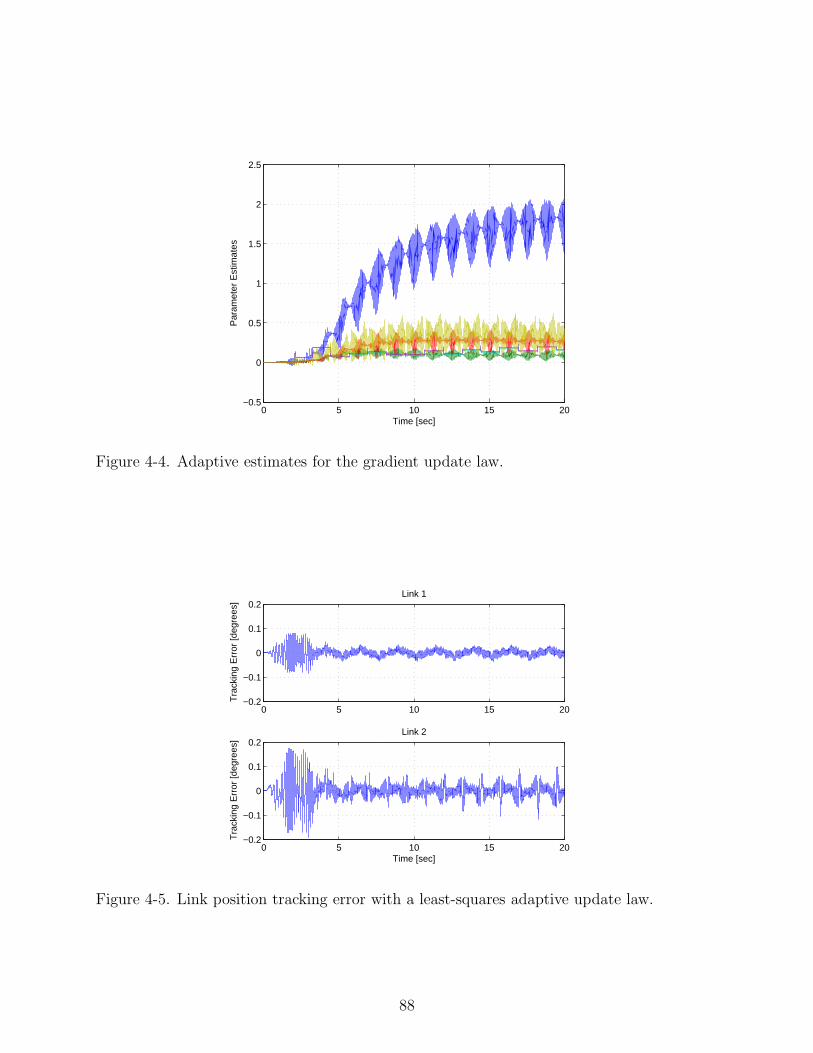
0 5 10 15 20−0.5

0

0.5

1

1.5

2

2.5

Par

amet

er E

stim

ates

Time [sec]

Figure 4-4. Adaptive estimates for the gradient update law.

0 5 10 15 20−0.2

−0.1

0

0.1

0.2

Tra

ckin

g E

rror

[deg

rees

]

Link 1

0 5 10 15 20−0.2

−0.1

0

0.1

0.2

Time [sec]

Tra

ckin

g E

rror

[deg

rees

]

Link 2

Figure 4-5. Link position tracking error with a least-squares adaptive update law.

88

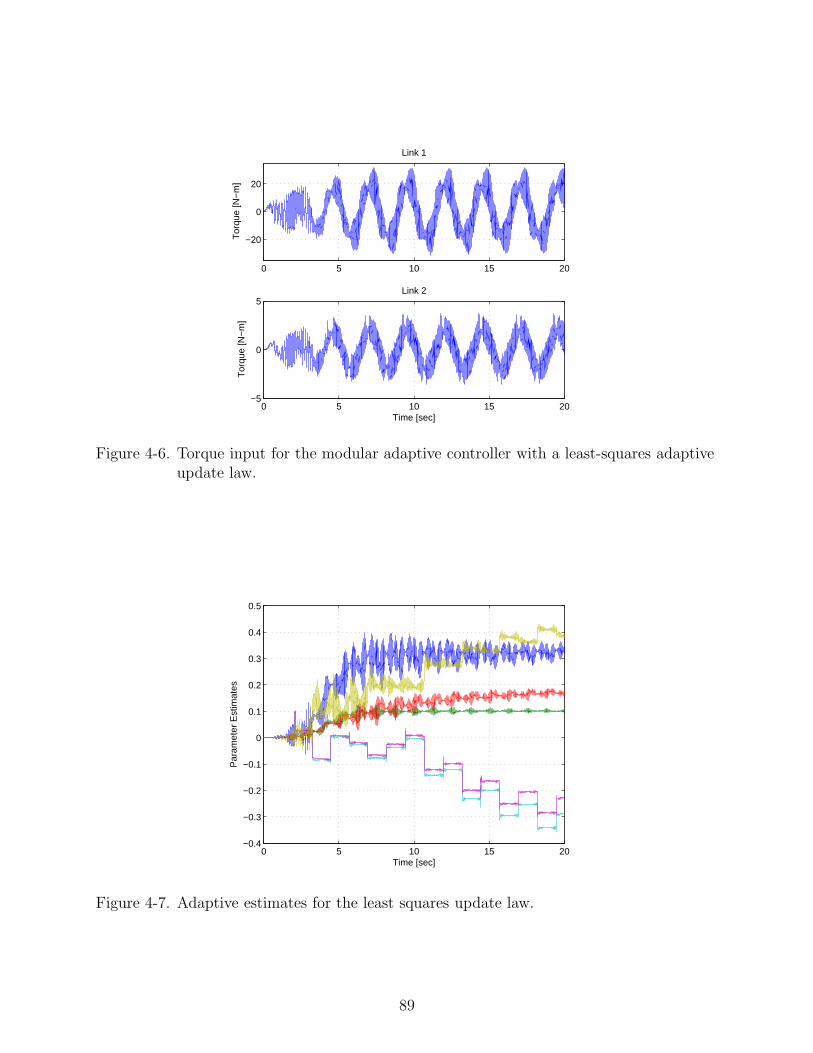
0 5 10 15 20

−20

0

20

Tor

que

[N−

m]

Link 1

0 5 10 15 20−5

0

5

Time [sec]

Tor

que

[N−

m]

Link 2

Figure 4-6. Torque input for the modular adaptive controller with a least-squares adaptiveupdate law.

0 5 10 15 20−0.4

−0.3

−0.2

−0.1

0

0.1

0.2

0.3

0.4

0.5

Par

amet

er E

stim

ates

Time [sec]

Figure 4-7. Adaptive estimates for the least squares update law.

89

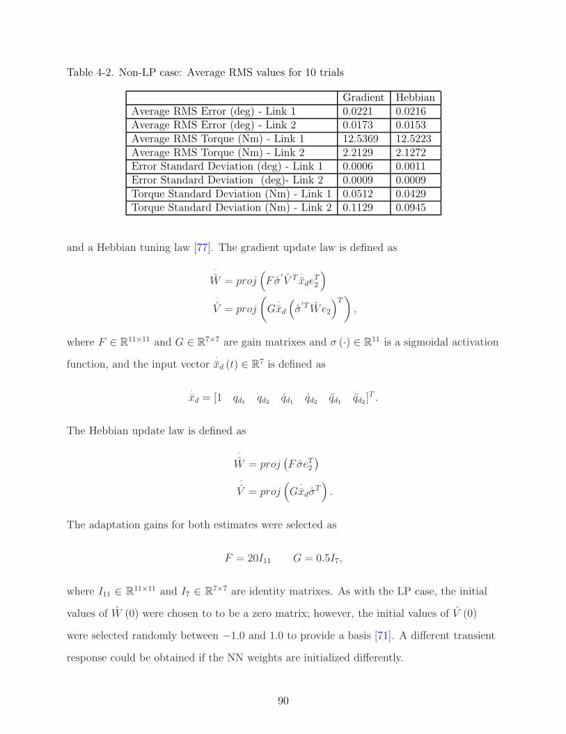
Table 4-2. Non-LP case: Average RMS values for 10 trials

Gradient HebbianAverage RMS Error (deg) - Link 1 0.0221 0.0216Average RMS Error (deg) - Link 2 0.0173 0.0153Average RMS Torque (Nm) - Link 1 12.5369 12.5223Average RMS Torque (Nm) - Link 2 2.2129 2.1272Error Standard Deviation (deg) - Link 1 0.0006 0.0011Error Standard Deviation (deg)- Link 2 0.0009 0.0009Torque Standard Deviation (Nm) - Link 1 0.0512 0.0429Torque Standard Deviation (Nm) - Link 2 0.1129 0.0945

and a Hebbian tuning law [77]. The gradient update law is defined as

·

W = proj(

F σ′

V T·

xdeT2

)

·

V = proj

(

G·

xd

(

σ′T W e2

)T)

,

where F ∈ R11×11 and G ∈ R7×7 are gain matrixes and σ (·) ∈ R11 is a sigmoidal activation

function, and the input vector·

xd (t) ∈ R7 is defined as

·

xd = [1 qd1 qd2 qd1 qd2 qd1 qd2 ]T .

The Hebbian update law is defined as

·

W = proj(

F σeT2

)

·

V = proj(

G·

xdσT)

.

The adaptation gains for both estimates were selected as

F = 20I11 G = 0.5I7,

where I11 ∈ R11×11 and I7 ∈ R7×7 are identity matrixes. As with the LP case, the initial

values of W (0) were chosen to to be a zero matrix; however, the initial values of V (0)

were selected randomly between −1.0 and 1.0 to provide a basis [71]. A different transient

response could be obtained if the NN weights are initialized differently.

90

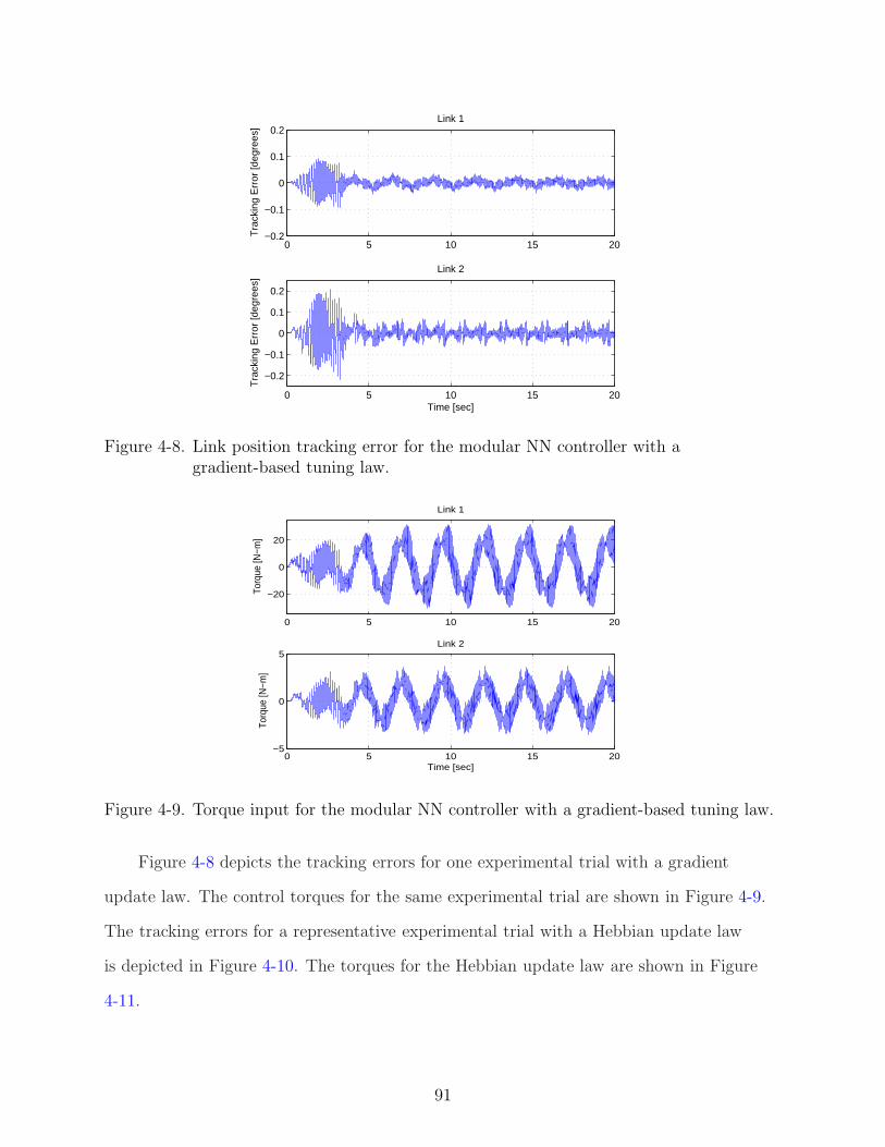
0 5 10 15 20−0.2

−0.1

0

0.1

0.2

Tra

ckin

g E

rror

[deg

rees

]

Link 1

0 5 10 15 20

−0.2

−0.1

0

0.1

0.2

Time [sec]

Tra

ckin

g E

rror

[deg

rees

]

Link 2

Figure 4-8. Link position tracking error for the modular NN controller with agradient-based tuning law.

0 5 10 15 20

−20

0

20

Torq

ue [N

−m]

Link 1

0 5 10 15 20−5

0

5

Time [sec]

Torq

ue [N

−m]

Link 2

Figure 4-9. Torque input for the modular NN controller with a gradient-based tuning law.

Figure 4-8 depicts the tracking errors for one experimental trial with a gradient

update law. The control torques for the same experimental trial are shown in Figure 4-9.

The tracking errors for a representative experimental trial with a Hebbian update law

is depicted in Figure 4-10. The torques for the Hebbian update law are shown in Figure

4-11.

91

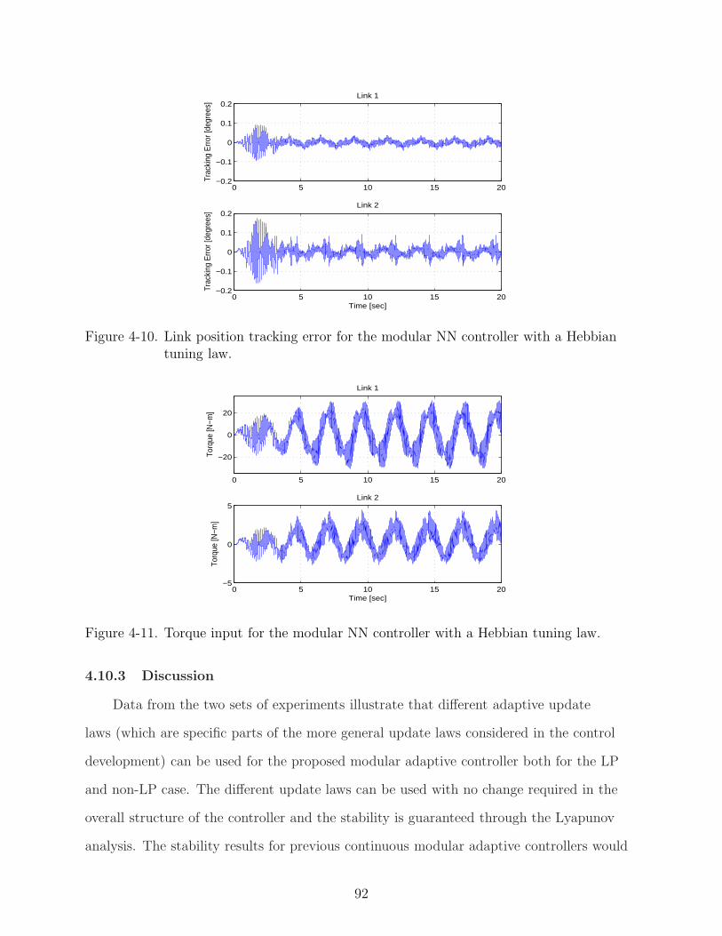
0 5 10 15 20−0.2

−0.1

0

0.1

0.2

Trac

king

Err

or [d

egre

es]

Link 1

0 5 10 15 20−0.2

−0.1

0

0.1

0.2

Time [sec]

Trac

king

Err

or [d

egre

es]

Link 2

Figure 4-10. Link position tracking error for the modular NN controller with a Hebbiantuning law.

0 5 10 15 20

−20

0

20

Torq

ue [N

−m]

Link 1

0 5 10 15 20−5

0

5

Time [sec]

Torq

ue [N

−m]

Link 2

Figure 4-11. Torque input for the modular NN controller with a Hebbian tuning law.

4.10.3 Discussion

Data from the two sets of experiments illustrate that different adaptive update

laws (which are specific parts of the more general update laws considered in the control

development) can be used for the proposed modular adaptive controller both for the LP

and non-LP case. The different update laws can be used with no change required in the

overall structure of the controller and the stability is guaranteed through the Lyapunov

analysis. The stability results for previous continuous modular adaptive controllers would

92

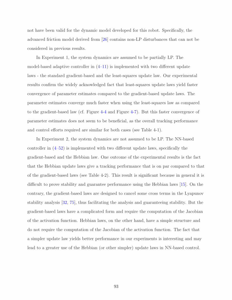
not have been valid for the dynamic model developed for this robot. Specifically, the

advanced friction model derived from [26] contains non-LP disturbances that can not be

considered in previous results.

In Experiment 1, the system dynamics are assumed to be partially LP. The

model-based adaptive controller in (4–11) is implemented with two different update

laws - the standard gradient-based and the least-squares update law. Our experimental

results confirm the widely acknowledged fact that least-squares update laws yield faster

convergence of parameter estimates compared to the gradient-based update laws. The

parameter estimates converge much faster when using the least-squares law as compared

to the gradient-based law (cf. Figure 4-4 and Figure 4-7). But this faster convergence of

parameter estimates does not seem to be beneficial, as the overall tracking performance

and control efforts required are similar for both cases (see Table 4-1).

In Experiment 2, the system dynamics are not assumed to be LP. The NN-based

controller in (4–52) is implemented with two different update laws, specifically the

gradient-based and the Hebbian law. One outcome of the experimental results is the fact

that the Hebbian update laws give a tracking performance that is on par compared to that

of the gradient-based laws (see Table 4-2). This result is significant because in general it is

difficult to prove stability and guarantee performance using the Hebbian laws [15]. On the

contrary, the gradient-based laws are designed to cancel some cross terms in the Lyapunov

stability analysis [32, 75], thus facilitating the analysis and guaranteeing stability. But the

gradient-based laws have a complicated form and require the computation of the Jacobian

of the activation function. Hebbian laws, on the other hand, have a simple structure and

do not require the computation of the Jacobian of the activation function. The fact that

a simpler update law yields better performance in our experiments is interesting and may

lead to a greater use of the Hebbian (or other simpler) update laws in NN-based control.

93

4.11 Conclusion

A RISE-based approach was presented to achieve modularity in the controller/update

law for a general class of multi-input systems. Specifically, for systems with structured

and unstructured uncertainties, a controller was employed that uses a model-based

feedforward adaptive term in conjunction with the RISE feedback term (see [19]). The

adaptive feedforward term was made modular by considering a generic form of the

adaptive update law and its corresponding parameter estimate. This generic form of

the update law was used to develop a new closed-loop error system, and the typical

RISE stability analysis was modified. New sufficient gain conditions were derived to

show asymptotic tracking of the desired link position. The class of RISE-based modular

adaptive controllers is then extended to include uncertain dynamic systems that do not

satisfy the LP assumption. Specifically, the result allows the NN weight tuning laws

to be determined from a developed generic update law (rather than being restricted to

a gradient update law). The modular adaptive control development is then applied to

Euler-Lagrange dynamic systems. An experimental section is included that illustrates the

concept.

94

CHAPTER 5COMPOSITE ADAPTIVE CONTROL FOR SYSTEMS WITH ADDITIVE

DISTURBANCES

5.1 Introduction

Applying the swapping approach to dynamics with additive disturbances is

problematic because the unknown disturbance terms also get filtered and included in

the filtered control input. This problem motivates the question of how can a prediction

error-based adaptive update law be developed for systems with additive disturbances.

To address this motivating question, a general Euler-Lagrange-like MIMO system

is considered with structured and unstructured uncertainties, and a gradient-based

composite adaptive update law is developed that is driven by both the tracking error and

the prediction error. The control development is based on the recent continuous Robust

Integral of the Sign of the Error (RISE) [19] technique that was originally developed in

[21] and [22]. The RISE architecture is adopted since this method can accommodate for

C2 disturbances and yield asymptotic stability. For example, the RISE technique was used

in [23] to develop a tracking controller for nonlinear systems in the presence of additive

disturbances and parametric uncertainties. Based on the well accepted heuristic notion

that the addition of system knowledge in the control structure yields better performance

and reduces control effort, model-based adaptive and neural network feedforward elements

were added to the RISE controller in [19] and [75], respectively. In comparison to these

approaches that used the RISE method in the feedback component of the controller, the

RISE structure is used in both the feedback and feedforward elements of the control

structure to enable, for the first time, the construction of a prediction error in the

presence of additive disturbances. Specifically, since the swapping method will result

in disturbances in the prediction error (the main obstacle that has previously limited this

development), an innovative use of the RISE structure is also employed in the prediction

error update (i.e., the filtered control input estimate). A block diagram indicating the

unique use of the RISE method in the control and the prediction error formulation is

95

provided in Figure 5-1. Sufficient gain conditions are developed under which this unique

double RISE controller guarantees semi-global asymptotic tracking. Experimental results

are presented to illustrate the performance of the proposed approach.

The asymptotic stability for the proposed RISE-based composite adaptive controller

comes at the expense of achieving semi-global stability which requires the initial condition

to be within a specified region of attraction that can be made larger by increasing

certain gains as subsequently discussed in Section 5.5. Development is also provided

that proves the prediction error is square integrable; yet, no conclusion can be drawn

about the convergence of the parameter estimation error due to the presence of filtered

additive disturbances in the prediction error. The proposed method uses a gradient-based

composite adaptive law with a fixed adaptation gain. Future efforts could also focus on

designing a composite law with least-squares estimation with time-varying adaptation gain

for the considered class of systems.

5.2 Dynamic System

Consider a class of MIMO nonlinear Euler-Lagrange systems of the following form:

x(m) = f(x, x, ..., x(m−1)) +G(x, x, ..., x(m−2))u+ h (t) (5–1)

where (·)(i) (t) denotes the ith derivative with respect to time, x(i) (t) ∈ Rn, i = 0, ..., m− 1

are the system states, u (t) ∈ Rn is the control input, f(

x, x, ..., x(m−1))

∈ Rn and

G(

x, x, ..., x(m−2))

∈ Rn×n are unknown nonlinear C2 functions, and h (t) ∈ Rn denotes

a general nonlinear disturbance (e.g., unmodeled effects). Throughout the chapter, |·|

denotes the absolute value of the scalar argument, ‖·‖ denotes the standard Euclidean

norm for a vector or the induced infinity norm for a matrix.

The subsequent development is based on the assumption that all the system states

are measurable outputs. Moreover, the following assumptions will be exploited in the

subsequent development.

96

Assumption 5-1: G (·) is symmetric positive definite, and satisfies the following

inequality ∀y(t) ∈ Rn:

g ‖y‖2 ≤ yTG−1y ≤ g(x, x, ..., x(m−2)) ‖y‖2 (5–2)

where g ∈ R is a known positive constant, and g(x, x, ..., x(m−2)) ∈ R is a known positive

function.

Assumption 5-2: The functions G−1(·) and f(·) are second order differentiable such that

G−1, G−1, G−1, f, f , f ∈ L∞ if x(i) (t) ∈ L∞, i = 0, 1, ..., m+ 1.

Assumption 5-3: The nonlinear disturbance term and its first two time derivatives (i.e.,

h, h, h) are bounded by known constants.

Assumption 5-4: The unknown nonlinearities G−1(·) and f(·) are linear in terms of

unknown constant system parameters (i.e., LP).

Assumption 5-5: The desired trajectory xd(t) ∈ Rn is assumed to be designed such that

x(i)d (t) ∈ L∞, i = 0, 1, ..., m + 2. The desired trajectory xd(t) need not be persistently

exciting and can be set to a constant value for the regulation problem.

5.3 Control Objective

The objective is to design a continuous composite adaptive controller which

ensures that the system state x (t) tracks a desired time-varying trajectory xd(t) despite

uncertainties and bounded disturbances in the dynamic model. To quantify this objective,

a tracking error, denoted by e1(t) ∈ Rn, is defined as

e1 , xd − x. (5–3)

97

To facilitate a compact presentation of the subsequent control development and stability

analysis, auxiliary error signals denoted by ei (t) ∈ Rn, i = 2, 3, ..., m are defined as

e2 , e1 + α1e1

e3 , e2 + α2e2 + e1

e4 , e3 + α3e3 + e2

...

ei , ei−1 + αi−1ei−1 + ei−2 (5–4)

...

em , em−1 + αm−1em−1 + em−2

where αi ∈ R, i = 1, 2, ..., m − 1 denote constant positive control gains. The error signals

ei (t) , i = 2, 3, ..., m can be expressed in terms of e1 (t) and its time derivatives as

ei =i−1∑

j=0

bi,je(j)1 , bi,i−1 = 1 (5–5)

where the constant coefficients bi,j ∈ R can be evaluated by substituting (5–5) in (5–4),

and comparing coefficients. A filtered tracking error [57], denoted by r(t) ∈ Rn, is also

defined as

r , em + αmem (5–6)

where αm ∈ R is a positive, constant control gain. The filtered tracking error r (t) is not

measurable since the expression in (5–6) depends on x(m).

5.4 Control Development

To develop the open-loop tracking error system, the filtered tracking error in (5–6) is

premultiplied by G−1 (·) to yield

G−1r = G−1em +G−1αmem. (5–7)

98

Substituting (5–5) in to (5–7) for em (t) yields

G−1r = G−1

m−1∑

j=0

bm,je(j+1)1 +G−1αmem. (5–8)

By separating the last term from the summation, (5–8) can also be expressed as

G−1r = G−1bm,m−1e(m)1 +G−1

m−2∑

j=0

bm,je(j+1)1 +G−1αmem. (5–9)

Using the fact that bm,m−1 = 1 and making substitutions from (5–1) and (5–3), the

expression in (5–9) is rewritten as

G−1r = G−1x(m)d −G−1f −G−1h− u+G−1

m−2∑

j=0

bm,je(j+1)1 +G−1αmem

which can be rearranged as

G−1r = Ydθ + S1 −G−1d h− u. (5–10)

In (5–10), the auxiliary function S1

(

x, x, ..., x(m−1), t)

∈ Rn is defined as

S1 , G−1

(

m−2∑

j=0

bm,je(j+1)1 + αmem

)

+G−1x(m)d −G−1

d x(m)d −G−1f +G−1

d fd −G−1h+G−1d h.

(5–11)

Also in (5–10), Ydθ ∈ Rn is defined as

Ydθ , G−1d x

(m)d −G−1

d fd (5–12)

where Yd(xd, xd, ..., x(m)d ) ∈ Rn×p is a desired regression matrix, and θ ∈ Rp contains the

constant unknown system parameters. In (5–12), the functions G−1d (xd, xd, ..., x

(m−2)d ) ∈

Rn×n and fd(xd, xd, ..., x(m−1)d ) ∈ Rn are defined as

G−1d , G−1(xd, xd, ..., x

(m−2)d ) (5–13)

fd , f(xd, xd, ..., x(m−1)d ).

99

The open-loop error system in (5–10) is typically written in a form similar to

G−1em = Ydθ + S1 −G−1αmem −G−1d h− u (5–14)

which can be obtained by substituting (5–6) into (5–10) for the filtered tracking error.

Although (5–10) and (5–14) are equivalent, the atypical form in (5–10) is used to facilitate

the subsequent closed-loop error system development and stability analysis. Specifically,

the subsequent RISE control method is designed based on the time derivative of the

control input. The design of the filtered tracking error in (5–6) is not necessary, but it

simplifies the subsequent development by allowing the closed-loop error system to be

expressed in terms of r(t) rather than em(t).

5.4.1 RISE-based Swapping

A measurable form of the prediction error ε (t) ∈ Rn is defined as the difference

between the filtered control input uf (t) ∈ Rn and the estimated filtered control input

uf (t) ∈ Rn as

ε , uf − uf (5–15)

where the filtered control input uf (t) ∈ Rn is generated by [3]

uf + ωuf = ωu , uf (0) = 0 (5–16)

where ω ∈ R is a known positive constant, and uf (t) ∈ Rn is subsequently designed. The

differential equation in (5–16) can be directly solved to yield

uf = v ∗ u (5–17)

where ∗ is used to denote the standard convolution operation, and the scalar function v (t)

is defined as

v , ωe−ωt. (5–18)

100

Using (5–1), the expression in (5–17) can be rewritten as

uf = v ∗(

G−1x(m) −G−1f −G−1h)

. (5–19)

Since the system dynamics in (5–1) include non-LP bounded disturbances h (t), they

also get filtered and included in the filtered control input in (5–19). To compensate for

the effects of these disturbances, the typical prediction error formulation is modified to

include a RISE-like structure in the design of the estimated filtered control input. With

this motivation, the structure of the open-loop prediction error system is engineered to

facilitate the RISE-based design of the estimated filtered control input.

Adding and subtracting the term G−1d x

(m)d +G−1

d fd +G−1d h to the expression in (5–19)

yields

uf = v∗(G−1d x

(m)d +G−1

d fd+G−1x(m)−G−1

d x(m)d −G−1f−G−1

d fd−G−1h+G−1

d h−G−1d h). (5–20)

Using (5–12), the expression in (5–20) is simplified as

uf = v ∗(

Ydθ + S − Sd −G−1d h)

(5–21)

where S(x, x, ..., x(m)), Sd(xd, xd, ..., x(m)d ) ∈ Rn are defined as

S , G−1x(m) −G−1f −G−1h (5–22)

Sd , G−1d x

(m)d −G−1

d fd −G−1d h. (5–23)

The expression in (5–21) is further simplified as

uf = Ydfθ + v ∗ S − v ∗ Sd + hf (5–24)

where the filtered regressor matrix Ydf(xd, xd, ..., x(m)d ) ∈ Rn×p is defined as

Ydf , v ∗ Yd (5–25)

101

and the disturbance hf (t) ∈ Rn is defined as

hf , −v ∗G−1d h.

The term v ∗ S(x, x, ..., x(m)) ∈ Rn in (5–24) depends on x(m). Using the following property

of convolution [57]:

g1 ∗ g2 = g1 ∗ g2 + g1 (0) g2 − g1g2 (0) (5–26)

an expression independent of x(m) can be obtained. Consider

v ∗ S = v ∗(

G−1x(m) −G−1f −G−1h)

which can be rewritten as

v ∗ S = v ∗ (d

dt(G−1x(m−1)) − G−1x(m−1) −G−1f −G−1h). (5–27)

Applying the property in (5–26) to the first term of (5–27) yields

v ∗ S = Sf +W (5–28)

where the state-dependent terms are included in the auxiliary function Sf(x, x, ..., x(m−1)) ∈

Rn, defined as

Sf , v ∗(

G−1x(m−1))

+ v (0)G−1x(m−1) − v ∗ G−1x(m−1) − v ∗G−1f − v ∗G−1h (5–29)

and the terms that depend on the initial states are included in W (t) ∈ Rn, defined as

W , −vG−1(

x (0) , x (0) , ..., x(m−2) (0))

x(m−1) (0) . (5–30)

Similarly, following the procedure in (5–27)-(5–30), the expression v ∗ Sd in (5–24) is

evaluated as

v ∗ Sd = Sdf +Wd (5–31)

102

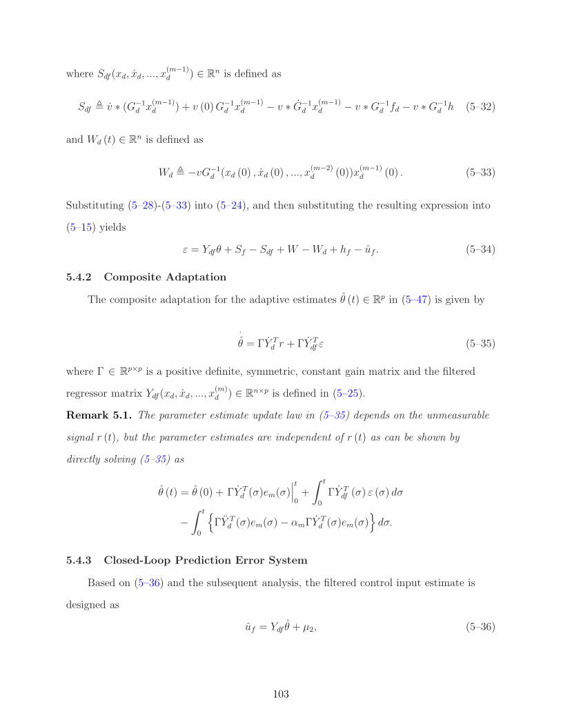
where Sdf (xd, xd, ..., x(m−1)d ) ∈ Rn is defined as

Sdf , v ∗ (G−1d x

(m−1)d ) + v (0)G−1

d x(m−1)d − v ∗ G−1

d x(m−1)d − v ∗G−1

d fd − v ∗G−1d h (5–32)

and Wd (t) ∈ Rn is defined as

Wd , −vG−1d (xd (0) , xd (0) , ..., x

(m−2)d (0))x

(m−1)d (0) . (5–33)

Substituting (5–28)-(5–33) into (5–24), and then substituting the resulting expression into

(5–15) yields

ε = Ydfθ + Sf − Sdf +W −Wd + hf − uf . (5–34)

5.4.2 Composite Adaptation

The composite adaptation for the adaptive estimates θ (t) ∈ Rp in (5–47) is given by

·

θ = ΓY Td r + ΓY T

df ε (5–35)

where Γ ∈ Rp×p is a positive definite, symmetric, constant gain matrix and the filtered

regressor matrix Ydf(xd, xd, ..., x(m)d ) ∈ Rn×p is defined in (5–25).

Remark 5.1. The parameter estimate update law in (5–35) depends on the unmeasurable

signal r (t), but the parameter estimates are independent of r (t) as can be shown by

directly solving (5–35) as

θ (t) = θ (0) + ΓY Td (σ)em(σ)

∣

∣

∣

t

0+

∫ t

0

ΓY Tdf (σ) ε (σ) dσ

−

∫ t

0

ΓY Td (σ)em(σ) − αmΓY T

d (σ)em(σ)

dσ.

5.4.3 Closed-Loop Prediction Error System

Based on (5–36) and the subsequent analysis, the filtered control input estimate is

designed as

uf = Ydf θ + µ2, (5–36)

103

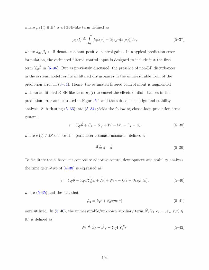
where µ2 (t) ∈ Rn is a RISE-like term defined as

µ2 (t) ,

∫ t

0

[k2ε(σ) + β2sgn(ε(σ))]dσ, (5–37)

where k2, β2 ∈ R denote constant positive control gains. In a typical prediction error

formulation, the estimated filtered control input is designed to include just the first

term Ydf θ in (5–36). But as previously discussed, the presence of non-LP disturbances

in the system model results in filtered disturbances in the unmeasurable form of the

prediction error in (5–34). Hence, the estimated filtered control input is augmented

with an additional RISE-like term µ2 (t) to cancel the effects of disturbances in the

prediction error as illustrated in Figure 5-1 and the subsequent design and stability

analysis. Substituting (5–36) into (5–34) yields the following closed-loop prediction error

system:

ε = Ydf θ + Sf − Sdf +W −Wd + hf − µ2 (5–38)

where θ (t) ∈ Rp denotes the parameter estimate mismatch defined as

θ , θ − θ. (5–39)

To facilitate the subsequent composite adaptive control development and stability analysis,

the time derivative of (5–38) is expressed as

ε = Ydf θ − YdfΓYTdf ε+ N2 +N2B − k2ε− β2sgn(ε), (5–40)

where (5–35) and the fact that

µ2 = k2ε+ β2sgn(ε) (5–41)

were utilized. In (5–40), the unmeasurable/unknown auxiliary term N2(e1, e2, ..., em, r, t) ∈

Rn is defined as

N2 , Sf − Sdf − YdfΓYTd r, (5–42)

104

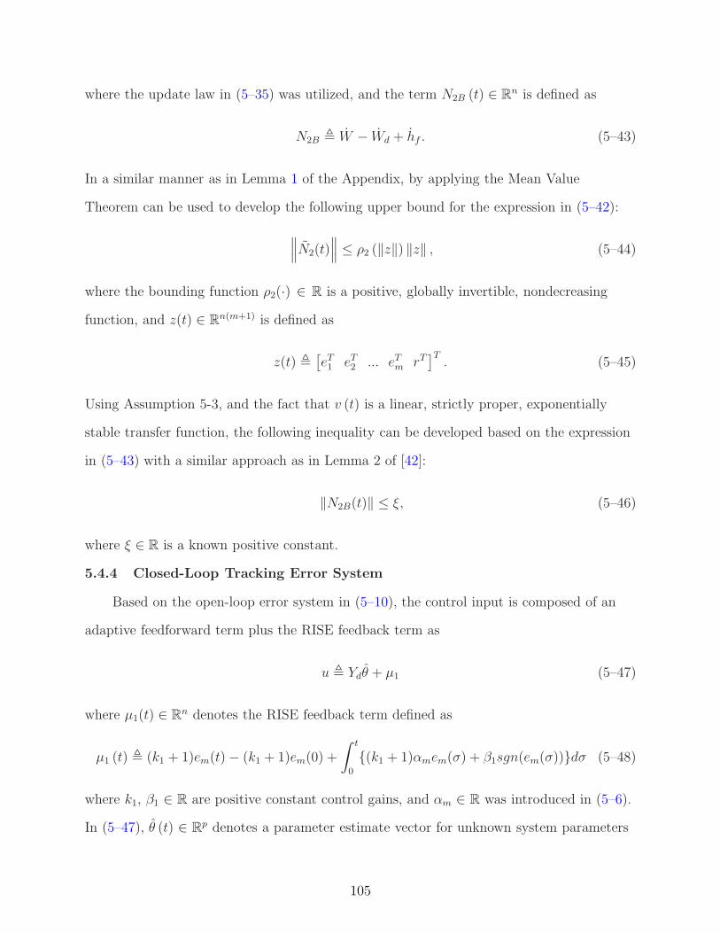
where the update law in (5–35) was utilized, and the term N2B (t) ∈ Rn is defined as

N2B , W − Wd + hf . (5–43)

In a similar manner as in Lemma 1 of the Appendix, by applying the Mean Value

Theorem can be used to develop the following upper bound for the expression in (5–42):

∥

∥

∥N2(t)

∥

∥

∥≤ ρ2 (‖z‖) ‖z‖ , (5–44)

where the bounding function ρ2(·) ∈ R is a positive, globally invertible, nondecreasing

function, and z(t) ∈ Rn(m+1) is defined as

z(t) ,[

eT1 eT

2 ... eTm rT

]T. (5–45)

Using Assumption 5-3, and the fact that v (t) is a linear, strictly proper, exponentially

stable transfer function, the following inequality can be developed based on the expression

in (5–43) with a similar approach as in Lemma 2 of [42]:

‖N2B(t)‖ ≤ ξ, (5–46)

where ξ ∈ R is a known positive constant.

5.4.4 Closed-Loop Tracking Error System

Based on the open-loop error system in (5–10), the control input is composed of an

adaptive feedforward term plus the RISE feedback term as

u , Ydθ + µ1 (5–47)

where µ1(t) ∈ Rn denotes the RISE feedback term defined as

µ1 (t) , (k1 + 1)em(t) − (k1 + 1)em(0) +

∫ t

0

(k1 + 1)αmem(σ) + β1sgn(em(σ))dσ (5–48)

where k1, β1 ∈ R are positive constant control gains, and αm ∈ R was introduced in (5–6).

In (5–47), θ (t) ∈ Rp denotes a parameter estimate vector for unknown system parameters

105

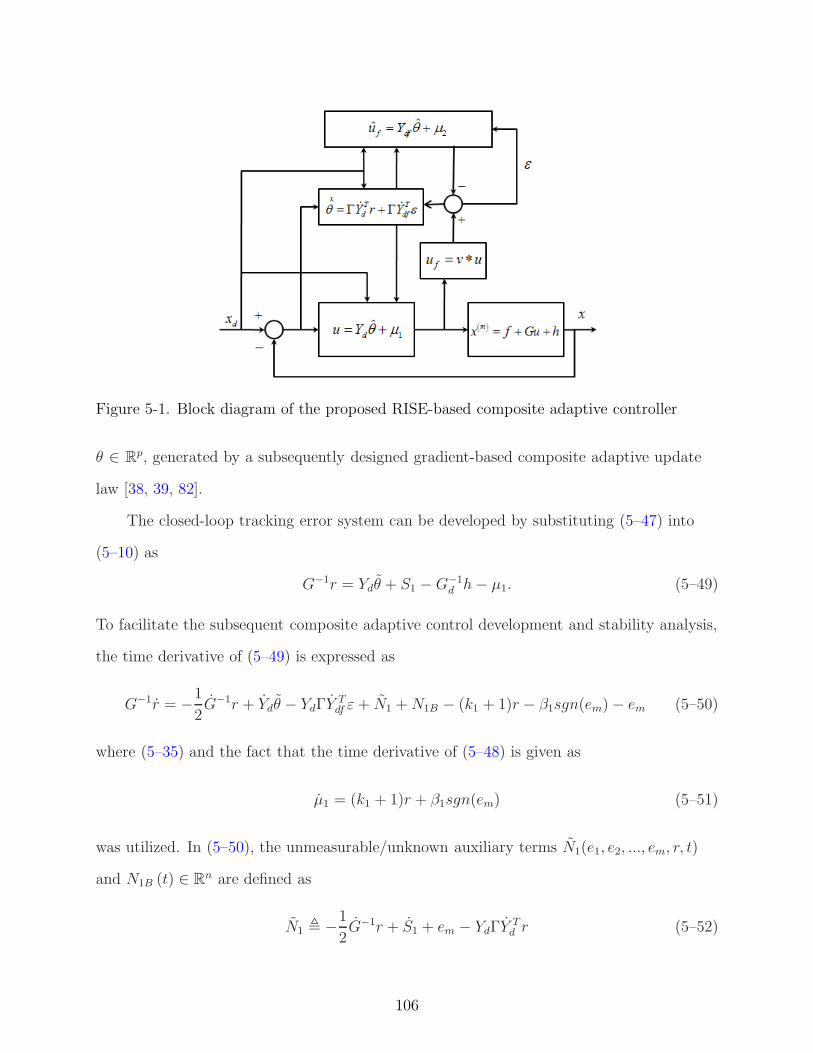
Figure 5-1. Block diagram of the proposed RISE-based composite adaptive controller

θ ∈ Rp, generated by a subsequently designed gradient-based composite adaptive update

law [38, 39, 82].

The closed-loop tracking error system can be developed by substituting (5–47) into

(5–10) as

G−1r = Ydθ + S1 −G−1d h− µ1. (5–49)

To facilitate the subsequent composite adaptive control development and stability analysis,

the time derivative of (5–49) is expressed as

G−1r = −1

2G−1r + Ydθ − YdΓY

Tdf ε+ N1 +N1B − (k1 + 1)r − β1sgn(em) − em (5–50)

where (5–35) and the fact that the time derivative of (5–48) is given as

µ1 = (k1 + 1)r + β1sgn(em) (5–51)

was utilized. In (5–50), the unmeasurable/unknown auxiliary terms N1(e1, e2, ..., em, r, t)

and N1B (t) ∈ Rn are defined as

N1 , −1

2G−1r + S1 + em − YdΓY

Td r (5–52)

106

where (5–35) was used, and

N1B , −G−1d h−G−1

d h. (5–53)

The structure of (5–50) and the introduction of the auxiliary terms in (5–52) and (5–53) is

motivated by the desire to segregate terms that can be upper bounded by state-dependent

terms and terms that can be upper bounded by constants. In a similar fashion as in

(5–44), the following upper bound can be developed for the expression in (5–52):

∥

∥

∥N1(t)

∥

∥

∥≤ ρ1 (‖z‖) ‖z‖ (5–54)

where the bounding function ρ1(·) ∈ R is a positive, globally invertible, nondecreasing

function, and z(t) ∈ Rn(m+1) was defined in (5–45). Using Assumptions 5-2 and 5-3, the

following inequalities can be developed based on the expression in (5–53) and its time

derivative:

‖N1B(t)‖ ≤ ζ1 ,∥

∥

∥N1B(t)

∥

∥

∥≤ ζ2 (5–55)

where ζi ∈ R, i = 1, 2 are known positive constants.

The RISE controller in (5–47) and (5–48), and sliding mode controllers (SMCs)

(e.g., see the classic results in [3, 12]) are the only methods that have been proven to

yield an asymptotic tracking result for an open-loop error system such as (5–10) where

additive bounded disturbances are present that are upper bounded by a constant. Other

approaches lack a mechanism to cancel the disturbance terms (these terms are typically

eliminated through nonlinear damping and yield a uniformly ultimately bounded (UUB)

result). SMC is a discontinuous control method that requires infinite control bandwidth

and a known upper bound on the disturbance term. Continuous modifications of SMC

reduce the stability result to UUB. The RISE control method in (5–47) and (5–48) is

continuous/differentiable (i.e., finite bandwidth) and requires a known upper bound on the

disturbance and the time derivative of the disturbance. Despite which feedback control

method is selected, the control challenge is that the disturbance term h(t) in (5–1) will be

included in the swapping (or torque filtering) method in the prediction error formulation

107

as shown in (5–34). This technical obstacle has prevented the development of any previous

composite adaptive controller for a dynamic system with added disturbances such as h(t).

The contribution of the current result is the development of the RISE-based swapping

method to enable the development of composite adaptive controllers for systems such as

(5–1). Specifically, the RISE-based swapping technique provides a means to cancel the

filtered disturbance terms in (5–34).

5.5 Stability Analysis

Theorem 5-1: The controller given in (5–47) and (5–48) in conjunction with the

composite adaptive update law in (5–35), where the prediction error is generated from

(5–15), (5–16), (5–36), and (5–37), ensures that all system signals are bounded under

closed-loop operation and that the position tracking error and the prediction error are

regulated in the sense that

‖e1(t)‖ → 0 and ‖ε(t)‖ → 0 as t→ ∞

provided the control gains k1 and k2 introduced in (5–48) and (5–37) are selected

sufficiently large based on the initial conditions of the system (see the subsequent proof),

and the following conditions are satisfied:

αm−1 >1

2, αm >

1

2, (5–56)

β1 > ζ1 +1

αm

ζ2 , β2 > ξ, (5–57)

where the gains αm−1 and αm were introduced in (5–4), β1 was introduced in (5–48), β2

was introduced in (5–37), ζ1 and ζ2 were introduced in (5–55), and ξ was introduced in

(5–46).

Proof: Let D ⊂ Rn(m+2)+p+2 be a domain containing y(t) = 0, where y(t) ∈

Rn(m+2)+p+2 is defined as

y , [zT εT√

P1

√

P2 θT ]T . (5–58)

108

In (5–58), the auxiliary function P1(t) ∈ R is defined as

P1 (t) , β1

n∑

i=1

|emi(0)| − em(0)TN1B(0) −

∫ t

0

L1(τ)dτ, (5–59)

where emi (0) ∈ R denotes the ith element of the vector em (0), and the auxiliary function

L1(t) ∈ R is defined as

L1 , rT (N1B − β1sgn(em)), (5–60)

where β1 ∈ R is a positive constant chosen according to the sufficient condition in (5–57).

Provided the sufficient condition introduced in (5–57) is satisfied, the following inequality

is obtained [22]:∫ t

0

L1(τ)dτ ≤ β1

n∑

i=1

|emi(0)| − em(0)TN1B(0). (5–61)

Hence, (5–61) can be used to conclude that P1(t) ≥ 0. Also in (5–58), the auxiliary

function P2(t) ∈ R is defined as

P2 (t) , −

∫ t

0

L2(τ)dτ, (5–62)

where the auxiliary function L2(t) ∈ R is defined as

L2 , εT (N2B − β2sgn(ε)), (5–63)

where β2 ∈ R is a positive constant chosen according to the sufficient condition in (5–57).

Provided the sufficient condition introduced in (5–57) is satisfied, then P2(t) ≥ 0.

Let VL(y, t) : D × [0,∞) → R be a continuously differentiable, positive definite

function defined as

VL(y, t) ,1

2

m∑

i=1

eTi ei +

1

2rTG−1r +

1

2εT ε+ P1 + P2 +

1

2θT Γ−1θ (5–64)

which satisfies the inequalities

U1(y) ≤ VL(y, t) ≤ U2(y) (5–65)

109

provided the sufficient conditions introduced in (5–57) are satisfied. In (5–65), the

continuous positive definite functions U1(y), U2(y) ∈ R are defined as U1(y) , λ1 ‖y‖2 and

U2(y) , λ2(x, x, ..., x(m−2)) ‖y‖2, where λ1, λ2(x, x, ..., x

(m−2)) ∈ R are defined as

λ1 ,1

2min

1, g, λmin

Γ−1

(5–66)

λ2 , max1

2g(x, x, ..., x(m−2)),

1

2λmax

Γ−1

, 1

where g, g(x, x, ..., x(m−2)) are introduced in (5–2), and λmin · and λmax · denote the

minimum and maximum eigenvalue of the arguments, respectively.

After using (5–4), (5–6), (5–35), (5–40), (5–50), (5–59), (5–60), (5–62) and (5–63), the

time derivative of (5–64) can be expressed as

VL(y, t) = −m∑

i=1

αieTi ei + eT

m−1em − rTr − k1rT r + rT Ydθ + rT N1

+ rTN1B − rTYdΓYTdf ε− β1r

T sgn(em) + εT Ydf θ (5–67)

+ εT N2 + εTN2B − k2εTε− εTYdfΓY

Tdf ε− β2ε

T sgn(ε)

− rT (N1B − β1sgn(em)) − εTN2B + εTβ2sgn(ε) − θT Γ−1(ΓY Td r + ΓY T

df ε).

After canceling the similar terms and using the fact that aT b ≤ 12(‖a‖2 + ‖b‖2) for some

a, b ∈ Rn, the expression in (5–67) is upper bounded as

VL(y, t) ≤ −

m∑

i=1

αieTi ei +

1

2‖em−1‖

2 +1

2‖em‖

2 − ‖r‖2

− k1 ‖r‖2 + rT N1 − rTYdΓY

Tdf ε+ εT N2 − k2ε

Tε− εTYdfΓYTdf ε.

Using the following upper bounds:

∥

∥

∥YdΓY

Tdf

∥

∥

∥≤ c1,

∥

∥

∥YdfΓY

Tdf

∥

∥

∥≤ c2,

110

where c1, c2 ∈ R are positive constants, VL(y, t) is upper bounded using the squares of the

components of z(t) as

VL(y, t) ≤ −λ3 ‖z‖2 − k1 ‖r‖

2 + ‖r‖∥

∥

∥N1

∥

∥

∥+ c1 ‖ε‖ ‖r‖ + ‖ε‖

∥

∥

∥N2

∥

∥

∥− (k2 − c2) ‖ε‖

2 , (5–68)

where

λ3 , minα1, α2, ..., αm−2, αm−1 −1

2, αm −

1

2, 1.

Letting

k2 = k2a + k2b

where k2a, k2b ∈ R are positive constants, and using the inequalities in (5–54) and (5–44),

the expression in (5–68) is upper bounded as

VL(y, t) ≤ −λ3 ‖z‖2 − k2b ‖ε‖

2 −[

k1 ‖r‖2 − ρ1(‖z‖) ‖r‖ ‖z‖

]

(5–69)

−[

(k2a − c2) ‖ε‖2 − (ρ2(‖z‖) + c1) ‖ε‖ ‖z‖

]

.

Completing the squares for the terms inside the brackets in (5–69) yields

VL(y, t) ≤ −λ3 ‖z‖2 − k2b ‖ε‖

2 +ρ2

1(‖z‖) ‖z‖2

4k1

+(ρ2(‖z‖) + c1)

2 ‖z‖2

4 (k2a − c2)

≤ −λ3 ‖z‖2 +

ρ2(‖z‖) ‖z‖2

4k− k2b ‖ε‖

2 , (5–70)

where k ∈ R is defined as

k ,k1 (k2a − c2)

max k1, (k2a − c2), k2a > c2 (5–71)

and ρ(·) ∈ R is a positive, globally invertible, nondecreasing function defined as

ρ2(‖z‖) , ρ21(‖z‖) + (ρ2(‖z‖) + c1)

2 .

111

The expression in (5–70) can be further upper bounded by a continuous, positive

semi-definite function

VL(y, t) ≤ −U(y) = −c∥

∥

∥

[

zT εT]T∥

∥

∥

2

∀y ∈ D (5–72)

for some positive constant c, where

D ,

y (t) ∈ Rn(m+2)+p+2 | ‖y‖ ≤ ρ−1

(

2√

λ3k)

.

Larger values of k will expand the size of the domain D. The inequalities in (5–65)

and (5–70) can be used to show that VL(y, t) ∈ L∞ in D; hence, ei(t) ∈ L∞ and

ε (t) , r(t), θ (t) ∈ L∞ in D. Given that ei(t) ∈ L∞ and r(t) ∈ L∞ in D, standard linear

analysis methods can be used to prove that ei(t) ∈ L∞ in D from (5–4) and (5–6). Since

ei(t) ∈ L∞, and r(t) ∈ L∞ in D, Assumption 5-5 can be used along with (5–3)-(5–6) to

conclude that x(i)(t) ∈ L∞, i = 0, 1, ..., m in D. Since θ (t) ∈ L∞ in D, (5–39) can be used

to prove that θ(t) ∈ L∞ in D. Since x(i)(t) ∈ L∞, i = 0, 1, ..., m in D, Assumption 5-2 can

be used to conclude that G−1(·) and f(·) ∈ L∞ in D. Thus, from (5–1) and Assumption

5-3, we can show that u(t) ∈ L∞ in D. Therefore, uf(t) ∈ L∞ in D, and hence, from

(5–15), uf(t) ∈ L∞ in D. Given that r(t) ∈ L∞ in D, (5–51) can be used to show that

µ1(t) ∈ L∞ in D, and since G−1(·) and f(·) ∈ L∞ in D, (5–50) can be used to show that

r(t) ∈ L∞ in D, and (5–40) can be used to show that ε(t) ∈ L∞ in D. Since ei(t) ∈ L∞,

r(t), and ε (t) ∈ L∞ in D, the definitions for U(y) and z(t) can be used to prove that U(y)

is uniformly continuous in D.

Let S ⊂ D denote a set defined as

S ,

y(t) ∈ D | U2(y(t)) < λ1

(

ρ−1(

2√

λ3k))2

. (5–73)

The region of attraction in (5–73) can be made arbitrarily large to include any initial

conditions by increasing the control gain k (i.e., a semi-global stability result). Theorem

112

8.4 of [63] can now be invoked to state that

c∥

∥

∥

[

zT εT]T∥

∥

∥

2

→ 0 as t→ ∞ ∀y(0) ∈ S. (5–74)

Based on the definition of z(t), (5–74) can be used to show that

‖e1(t)‖ → 0 as t→ ∞ ∀y(0) ∈ S (5–75)

‖ε(t)‖ → 0 as t→ ∞ ∀y(0) ∈ S.

5.6 Experiment

As in Chapter 2, the testbed depicted in Figure 2-1 was used to implement the

developed controller. The desired link trajectory is selected as follows (in degrees):

qd(t) = 60.0 sin(1.2t)(1 − exp(−0.01t3)). (5–76)

For all experiments, the rotor velocity signal is obtained by applying a standard backwards

difference algorithm to the position signal. The integral structure for the RISE term

in (5–48) was computed on-line via a standard trapezoidal algorithm. The parameter

estimates were all initialized to zero. In practice, the adaptive estimates would be

initialized to a best-guess estimate of the values. Initializing the estimates to zero was

done to test a scenario of no parameter knowledge. In addition, all the states were

initialized to zero. The following control gains and best guess estimates were used to

implement the controller in (5–47) and (5–48) in conjunction with the composite adaptive

update law in (5–35), where the prediction error is generated from (5–15), (5–16), (5–36),

and (5–37):

k1 = 70, β1 = 50, α1 = 20, α2 = 10, Γ = diag 4, 0.9, 0.9, 2

k2 = 400, β2 = 1, ω = 10, γ2 = 50, γ3 = 1, γ5 = 50. (5–77)

113

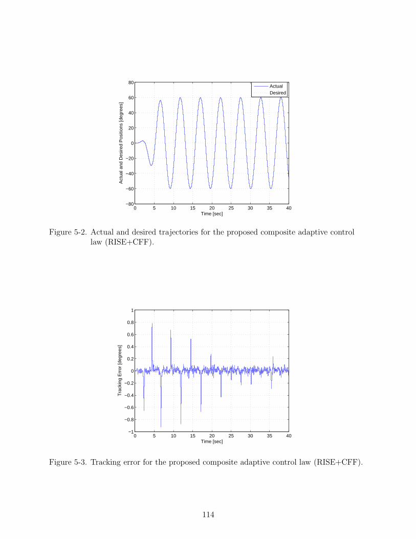
0 5 10 15 20 25 30 35 40−80

−60

−40

−20

0

20

40

60

80

Act

ual a

nd D

esire

d P

ositi

ons

[deg

rees

]

Time [sec]

ActualDesired

Figure 5-2. Actual and desired trajectories for the proposed composite adaptive controllaw (RISE+CFF).

0 5 10 15 20 25 30 35 40−1

−0.8

−0.6

−0.4

−0.2

0

0.2

0.4

0.6

0.8

1

Tra

ckin

g E

rror

[deg

rees

]

Time [sec]

Figure 5-3. Tracking error for the proposed composite adaptive control law (RISE+CFF).

114

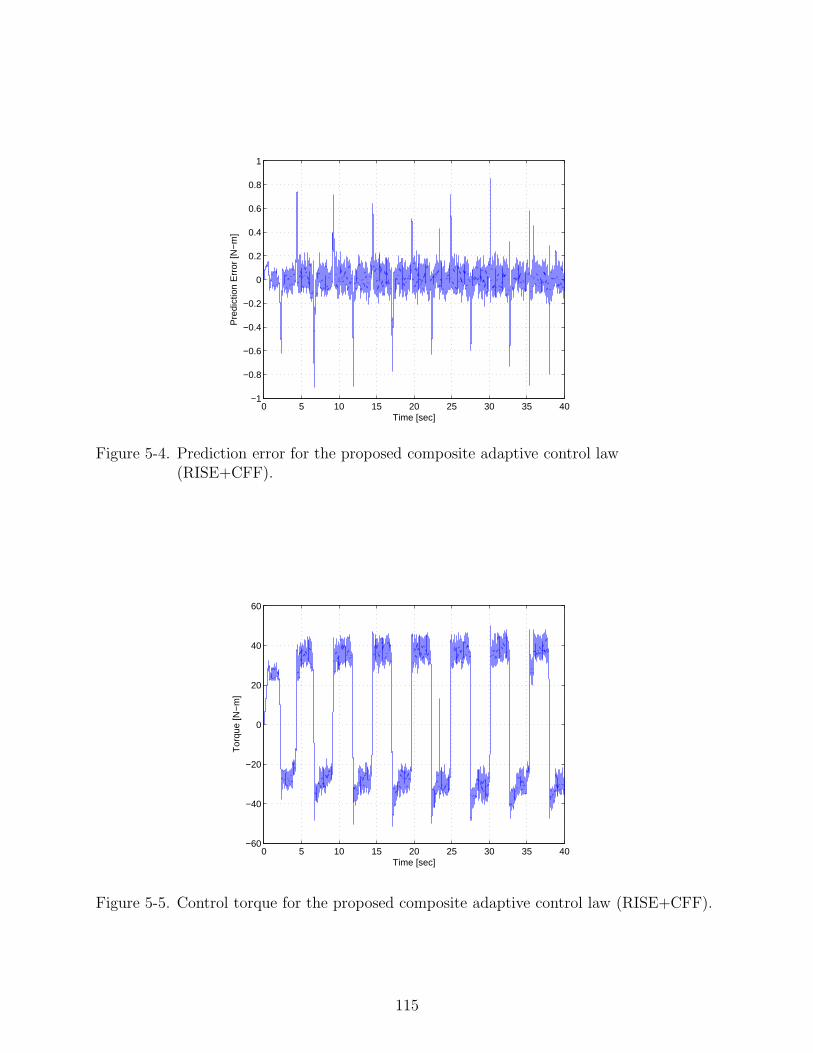
0 5 10 15 20 25 30 35 40−1

−0.8

−0.6

−0.4

−0.2

0

0.2

0.4

0.6

0.8

1

Pre

dict

ion

Err

or [N

−m

]

Time [sec]

Figure 5-4. Prediction error for the proposed composite adaptive control law(RISE+CFF).

0 5 10 15 20 25 30 35 40−60

−40

−20

0

20

40

60

Tor

que

[N−

m]

Time [sec]

Figure 5-5. Control torque for the proposed composite adaptive control law (RISE+CFF).

115

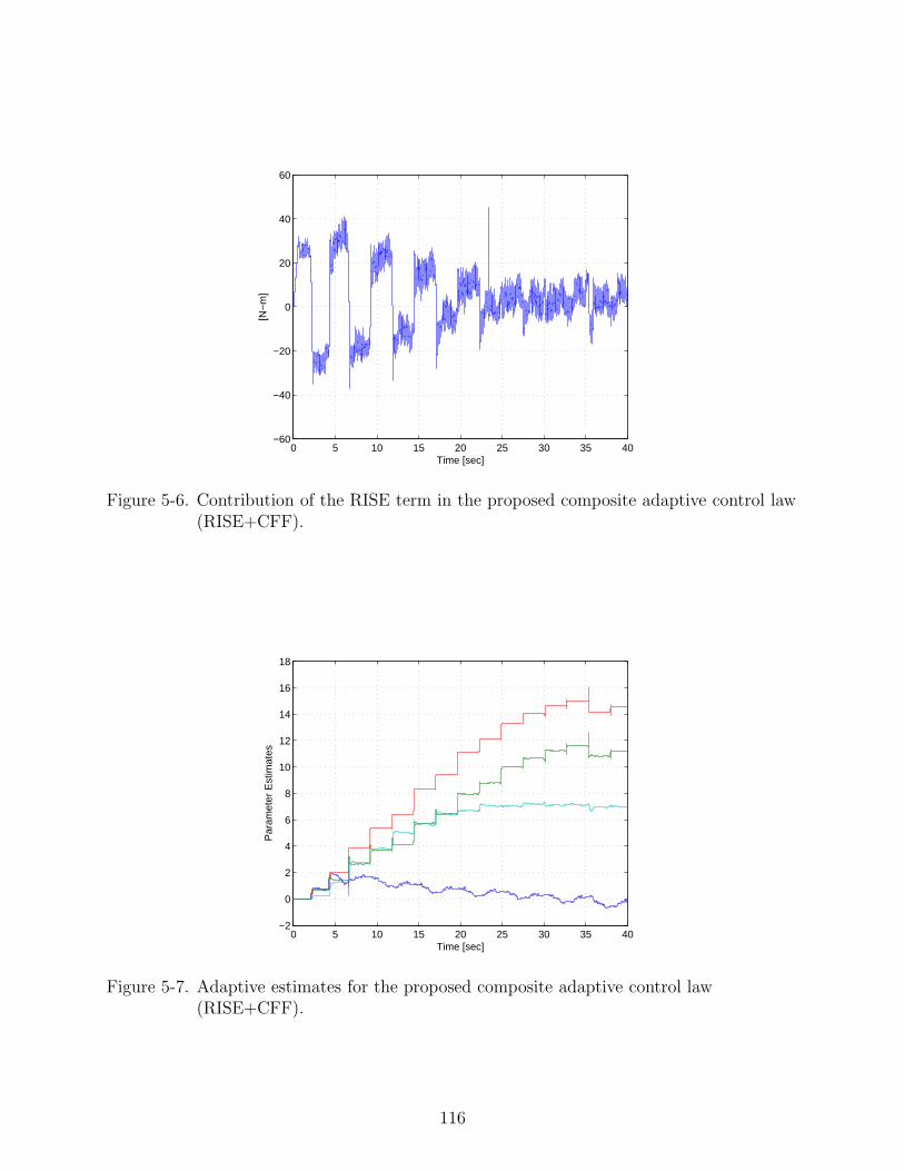
0 5 10 15 20 25 30 35 40−60

−40

−20

0

20

40

60

[N−

m]

Time [sec]

Figure 5-6. Contribution of the RISE term in the proposed composite adaptive control law(RISE+CFF).

0 5 10 15 20 25 30 35 40−2

0

2

4

6

8

10

12

14

16

18

Par

amet

er E

stim

ates

Time [sec]

Figure 5-7. Adaptive estimates for the proposed composite adaptive control law(RISE+CFF).

116

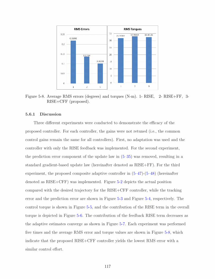
Figure 5-8. Average RMS errors (degrees) and torques (N-m). 1- RISE, 2- RISE+FF, 3-RISE+CFF (proposed).

5.6.1 Discussion

Three different experiments were conducted to demonstrate the efficacy of the

proposed controller. For each controller, the gains were not retuned (i.e., the common

control gains remain the same for all controllers). First, no adaptation was used and the

controller with only the RISE feedback was implemented. For the second experiment,

the prediction error component of the update law in (5–35) was removed, resulting in a

standard gradient-based update law (hereinafter denoted as RISE+FF). For the third

experiment, the proposed composite adaptive controller in (5–47)-(5–48) (hereinafter

denoted as RISE+CFF) was implemented. Figure 5-2 depicts the actual position

compared with the desired trajectory for the RISE+CFF controller, while the tracking

error and the prediction error are shown in Figure 5-3 and Figure 5-4, respectively. The

control torque is shown in Figure 5-5, and the contribution of the RISE term in the overall

torque is depicted in Figure 5-6. The contribution of the feedback RISE term decreases as

the adaptive estimates converge as shown in Figure 5-7. Each experiment was performed

five times and the average RMS error and torque values are shown in Figure 5-8, which

indicate that the proposed RISE+CFF controller yields the lowest RMS error with a

similar control effort.

117

5.7 Conclusion

A novel approach for the design of a gradient-based composite adaptive controller was

proposed for generic MIMO systems subjected to bounded disturbances. A model-based

feedforward adaptive component was used in conjunction with the RISE feedback, where

the adaptive estimates were generated using a composite update law driven by both

the tracking and prediction error with the motivation of using more information in the

adaptive update law. To account for the effects of non-LP disturbances, the typical

prediction error formulation was modified to include a second RISE-like term in the

estimated filtered control input design. Using a Lyapunov stability analysis, sufficient

gain conditions were derived under which the proposed controller yields semi-global

asymptotic stability. The current development, as well as all previous RISE controllers,

require full-state feedback. The development of an output feedback result remains an open

problem. Experiments on a rotating disk with externally applied friction indicate that the

proposed method yields better tracking performance with a similar control effort.

118

CHAPTER 6COMPOSITE ADAPTATION FOR NN-BASED CONTROLLERS

6.1 Introduction

This chapter presents the first ever attempt to develop a prediction error-based

composite adaptive NN controller for an Euler-Lagrange second-order dynamic system

using the recent continuous Robust Integral of the Sign of the Error (RISE) [19] technique

that was originally developed in [21] and [22]. The RISE architecture is adopted since

this method can accommodate for C2 disturbances and yield asymptotic stability.

The RISE technique was used in [75] to prove the first ever asymptotic result for a

NN-based controller using a continuous feedback. In this chapter, the RISE feedback is

used in conjunction with a NN feedfoward element similar to [75], however, unlike the

typical tracking error-based gradient update law used in [75], the result in this chapter

uses a composite update law driven by both the tracking and the prediction error. In

order to compensate for the effect of NN reconstruction error, an innovative use of the

RISE structure is also employed in the prediction error update (i.e., the filtered control

input estimate). A block diagram indicating the unique use of the RISE method in

the control and the prediction error formulation is provided in Figure 6-1. Sufficient

gain conditions are derived using a Lyapunov-based stability analysis under which this

unique double-RISE control strategy yields a semi-global asymptotic stability for the

system tracking errors and the prediction error, while all other signals and the control

input are shown to be bounded. Since a multi-layer NN includes the first layer weight

estimate inside of a nonlinear activation function, proving that the NN weight estimates

are bounded is a challenging task. A projection algorithm is used to guarantee the

boundedness of the weight estimates. However, if instead a single-layer NN is used,

projection is not required and the weight estimates can be shown bounded via the stability

analysis. The control development in this chapter can be easily simplified for a single-layer

NN by choosing fixed first layer weights.

119

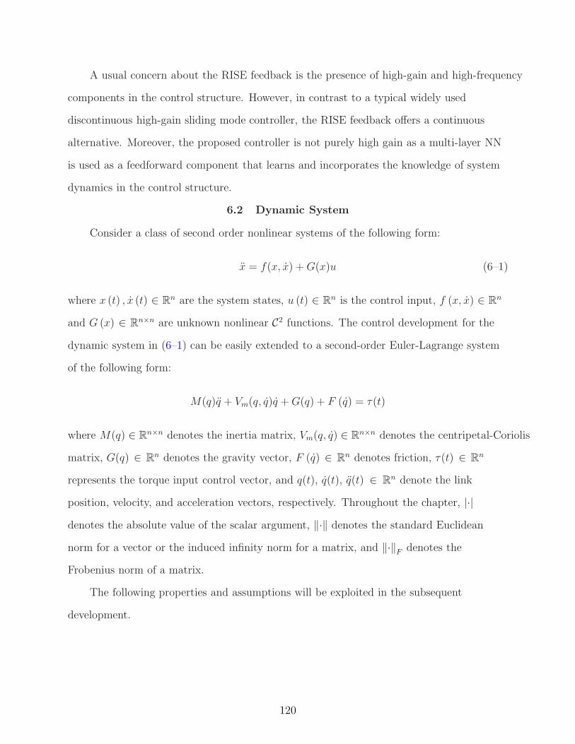
A usual concern about the RISE feedback is the presence of high-gain and high-frequency

components in the control structure. However, in contrast to a typical widely used

discontinuous high-gain sliding mode controller, the RISE feedback offers a continuous

alternative. Moreover, the proposed controller is not purely high gain as a multi-layer NN

is used as a feedforward component that learns and incorporates the knowledge of system

dynamics in the control structure.

6.2 Dynamic System

Consider a class of second order nonlinear systems of the following form:

x = f(x, x) +G(x)u (6–1)

where x (t) , x (t) ∈ Rn are the system states, u (t) ∈ Rn is the control input, f (x, x) ∈ Rn

and G (x) ∈ Rn×n are unknown nonlinear C2 functions. The control development for the

dynamic system in (6–1) can be easily extended to a second-order Euler-Lagrange system

of the following form:

M(q)q + Vm(q, q)q +G(q) + F (q) = τ(t)

where M(q) ∈ Rn×n denotes the inertia matrix, Vm(q, q) ∈ Rn×n denotes the centripetal-Coriolis

matrix, G(q) ∈ Rn denotes the gravity vector, F (q) ∈ Rn denotes friction, τ(t) ∈ Rn

represents the torque input control vector, and q(t), q(t), q(t) ∈ Rn denote the link

position, velocity, and acceleration vectors, respectively. Throughout the chapter, |·|

denotes the absolute value of the scalar argument, ‖·‖ denotes the standard Euclidean

norm for a vector or the induced infinity norm for a matrix, and ‖·‖F denotes the

Frobenius norm of a matrix.

The following properties and assumptions will be exploited in the subsequent

development.

120

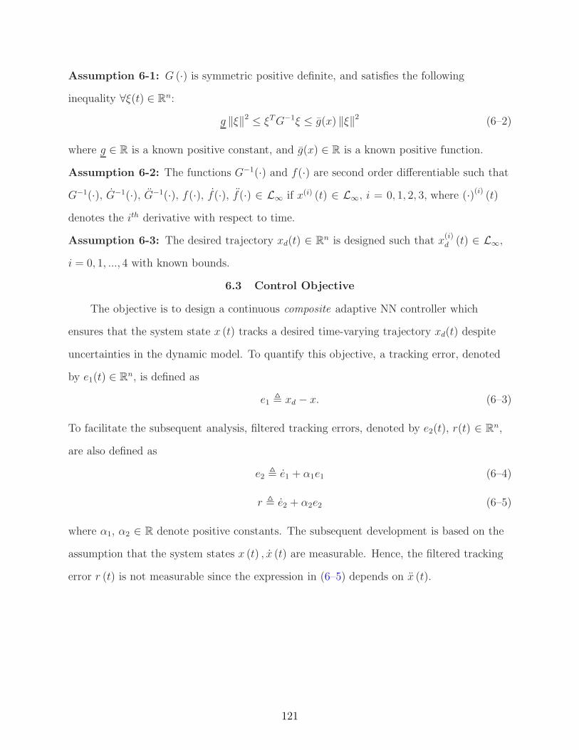
Assumption 6-1: G (·) is symmetric positive definite, and satisfies the following

inequality ∀ξ(t) ∈ Rn:

g ‖ξ‖2 ≤ ξTG−1ξ ≤ g(x) ‖ξ‖2 (6–2)

where g ∈ R is a known positive constant, and g(x) ∈ R is a known positive function.

Assumption 6-2: The functions G−1(·) and f(·) are second order differentiable such that

G−1(·), G−1(·), G−1(·), f(·), f(·), f(·) ∈ L∞ if x(i) (t) ∈ L∞, i = 0, 1, 2, 3, where (·)(i) (t)

denotes the ith derivative with respect to time.

Assumption 6-3: The desired trajectory xd(t) ∈ Rn is designed such that x(i)d (t) ∈ L∞,

i = 0, 1, ..., 4 with known bounds.

6.3 Control Objective

The objective is to design a continuous composite adaptive NN controller which

ensures that the system state x (t) tracks a desired time-varying trajectory xd(t) despite

uncertainties in the dynamic model. To quantify this objective, a tracking error, denoted

by e1(t) ∈ Rn, is defined as

e1 , xd − x. (6–3)

To facilitate the subsequent analysis, filtered tracking errors, denoted by e2(t), r(t) ∈ Rn,

are also defined as

e2 , e1 + α1e1 (6–4)

r , e2 + α2e2 (6–5)

where α1, α2 ∈ R denote positive constants. The subsequent development is based on the

assumption that the system states x (t) , x (t) are measurable. Hence, the filtered tracking

error r (t) is not measurable since the expression in (6–5) depends on x (t).

121

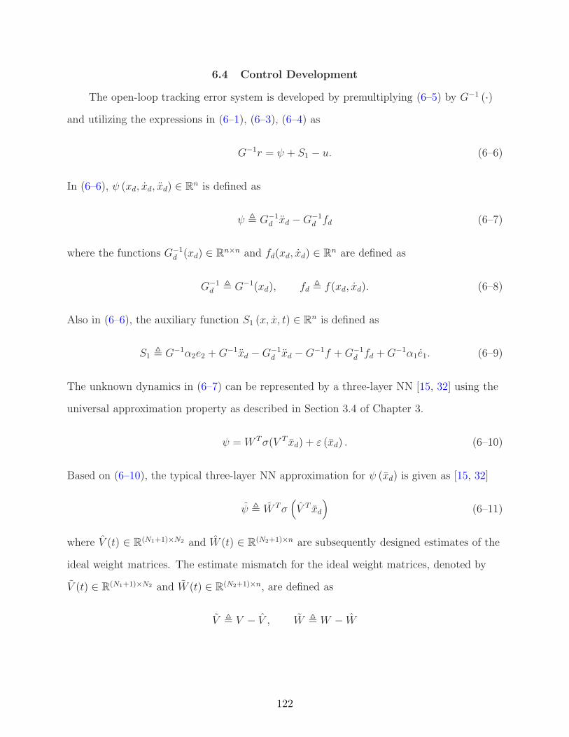
6.4 Control Development

The open-loop tracking error system is developed by premultiplying (6–5) by G−1 (·)

and utilizing the expressions in (6–1), (6–3), (6–4) as

G−1r = ψ + S1 − u. (6–6)

In (6–6), ψ (xd, xd, xd) ∈ Rn is defined as

ψ , G−1d xd −G−1

d fd (6–7)

where the functions G−1d (xd) ∈ Rn×n and fd(xd, xd) ∈ Rn are defined as

G−1d , G−1(xd), fd , f(xd, xd). (6–8)

Also in (6–6), the auxiliary function S1 (x, x, t) ∈ Rn is defined as

S1 , G−1α2e2 +G−1xd −G−1d xd −G−1f +G−1

d fd +G−1α1e1. (6–9)

The unknown dynamics in (6–7) can be represented by a three-layer NN [15, 32] using the

universal approximation property as described in Section 3.4 of Chapter 3.

ψ = W Tσ(V T xd) + ε (xd) . (6–10)

Based on (6–10), the typical three-layer NN approximation for ψ (xd) is given as [15, 32]

ψ , W Tσ(

V T xd

)

(6–11)

where V (t) ∈ R(N1+1)×N2 and W (t) ∈ R(N2+1)×n are subsequently designed estimates of the

ideal weight matrices. The estimate mismatch for the ideal weight matrices, denoted by

V (t) ∈ R(N1+1)×N2 and W (t) ∈ R(N2+1)×n, are defined as

V , V − V , W , W − W

122

and the mismatch for the hidden-layer output error for a given xd(t), denoted by σ(xd) ∈

RN2+1, is defined as

σ , σ − σ = σ(

V T xd

)

− σ(

V T xd

)

. (6–12)

Property 6-1: (Taylor Series Approximation) The Taylor series expansion for σ(

V T xd

)

for a given xd (t) may be written as [15, 32]

σ(

V T xd

)

= σ(

V T xd

)

+ σ′

(

V T xd

)

V T xd +O(

V T xd

)2

(6–13)

where σ′

(

V T xd

)

≡ dσ(

V T xd

)

/d(

V T xd

)

|V T xd=V T xd, and O

(

V T xd

)2

denotes the

higher order terms. After substituting (6–13) into (6–12), the following expression can be

obtained

σ = σ′

V T xd +O(

V T xd

)2

(6–14)

where σ′

, σ′

(

V T xd

)

.

Based on the open-loop error system in (6–6), the control input is composed of a NN

estimate term plus the RISE feedback term as [75]

u , ψ + µ1 (6–15)

where ψ(t) ∈ Rn denotes a first ever, subsequently designed, prediction-error based

NN feedfoward term. In (6–15), µ1(t) ∈ Rn denotes the RISE feedback term defined as

[21, 22, 75]

µ1 (t) , (k1 + 1)e2(t) − (k1 + 1)e2(0) +

∫ t

0

(k1 + 1)α2e2(σ) + β1sgn(e2(σ))dσ (6–16)

where k1, β1 ∈ R are positive constant control gains, α2 ∈ R was introduced in (6–5), and

sgn (·) denotes the signum function defined as

sgn(e2) , [sgn(e21) sgn(e22) ... sgn(e2i) ... sgn(e2n

)]T .

123

The closed-loop tracking error system can be developed by substituting (6–15) into (6–6)

as

G−1r = ψ − ψ + S1 − µ1. (6–17)

To facilitate the subsequent composite adaptive control development and stability analysis,

(6–10) and (6–11) are used to express the time derivative of (6–17) as

G−1r = −G−1r +W Tσ′(

V T xd

)

V T·

xd −·

W Tσ(V T xd) − W Tσ′

(V T xd)·

V T xd (6–18)

− W Tσ′

(V T xd)VT

·

xd + ε+ S1 − µ1.

After adding and subtracting the terms W T σ′

V T·

xd + W T σ′

V T·

xd to (6–18), the following

expression can be obtained:

G−1r = −G−1r + W T σ′

V T·

xd + W T σ′

V T·

xd +W Tσ′

V T·

xd −W T σ′

V T·

xd (6–19)

− W T σ′

V T·

xd + S1 −·

W T σ − W T σ′

·

V T xd + ε− µ1

where the notations σ(

V T xd

)

and σ′

(

V T xd

)

are introduced in (6–12) and (6–14),

respectively.

6.4.1 Swapping

In this section, the swapping procedure is used to generate a measurable form of

a prediction error that relates to the function mismatch error (i.e., ψ (t) − ψ (t)). A

measurable form of the prediction error η (t) ∈ Rn is defined as the difference between a

filtered control input uf (t) ∈ Rn and an estimated filtered control input uf (t) ∈ R

n as

η , uf − uf (6–20)

where the filtered control input is generated from the stable first order differential

equation

uf + ωuf = ωu , uf (0) = 0 (6–21)

124

where ω ∈ R is a known positive constant. The differential equation in (6–21) can be

expressed as a convolution as

uf = v ∗ u (6–22)

where ∗ is used to denote the standard convolution operation, and the scalar function v (t)

is defined as

v , ωe−ωt. (6–23)

Using (6–1), the expression in (6–22) can be rewritten as

uf = v ∗(

G−1x−G−1f)

. (6–24)

The construction of a NN-based controller to approximate the unknown system dynamics

in (6–24) will inherently result in a residual function reconstruction error ε (xd). The

presence of the reconstruction error has been the technical obstacle that has prevented

the development of composite adaptation laws for NNs. To compensate for the effects

of the reconstruction error, the typical prediction error formulation is modified to

include a RISE-like structure in the design of the estimated filtered control input. With

this motivation, the open-loop prediction error system is engineered to facilitate the

RISE-based design of the estimated filtered control input.

Adding and subtracting the term v ∗(

G−1d xd +G−1

d fd

)

to the expression in (6–24),

and using (6–7) yields

uf = v ∗ (ψ + S − Sd) (6–25)

where S(x, x, x), Sd(xd, xd, xd) ∈ Rn are defined as

S , G−1x−G−1f (6–26)

Sd , G−1d xd −G−1

d fd. (6–27)

The expression in (6–25) is further simplified as

uf = v ∗ ψ + v ∗ S − v ∗ Sd. (6–28)

125

The term v ∗ S(x, x, x) ∈ Rn in (6–28) depends on x (t). Using the following property of

convolution [57]:

g1 ∗ g2 = g1 ∗ g2 + g1 (0) g2 − g1g2 (0) (6–29)

an expression independent of x (t) can be obtained as

v ∗ S = Sf +D (6–30)

where the state-dependent terms are included in the auxiliary function Sf(x, x) ∈ Rn,

defined as

Sf , v ∗(

G−1x)

+ v (0)G−1x− v ∗ G−1x− v ∗G−1f (6–31)

and the terms that depend on the initial states are included in D (t) ∈ Rn, defined as

D , −vG−1 (x (0)) x (0) . (6–32)

Similarly, the expression v ∗ Sd (xd, xd, xd) in (6–28) is evaluated as

v ∗ Sd = Sdf +Dd (6–33)

where Sdf (xd, xd) ∈ Rn is defined as

Sdf , v ∗ (G−1d xd) + v (0)G−1

d xd − v ∗ G−1d xd − v ∗G−1

d fd (6–34)

and Dd (t) ∈ Rn is defined as

Dd , −vG−1d (xd (0))xd (0) . (6–35)

Substituting (6–30)-(6–35) into (6–28), and then substituting the resulting expression into

(6–20) yields

η = v ∗ ψ + Sf − Sdf +D −Dd − uf . (6–36)

126

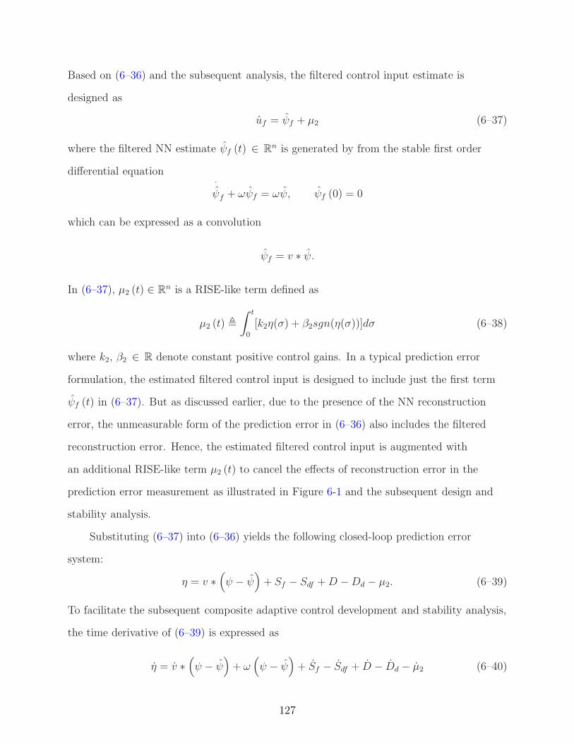
Based on (6–36) and the subsequent analysis, the filtered control input estimate is

designed as

uf = ψf + µ2 (6–37)

where the filtered NN estimate ψf (t) ∈ Rn is generated by from the stable first order

differential equation·

ψf + ωψf = ωψ, ψf (0) = 0

which can be expressed as a convolution

ψf = v ∗ ψ.

In (6–37), µ2 (t) ∈ Rn is a RISE-like term defined as

µ2 (t) ,

∫ t

0

[k2η(σ) + β2sgn(η(σ))]dσ (6–38)

where k2, β2 ∈ R denote constant positive control gains. In a typical prediction error

formulation, the estimated filtered control input is designed to include just the first term

ψf (t) in (6–37). But as discussed earlier, due to the presence of the NN reconstruction

error, the unmeasurable form of the prediction error in (6–36) also includes the filtered

reconstruction error. Hence, the estimated filtered control input is augmented with

an additional RISE-like term µ2 (t) to cancel the effects of reconstruction error in the

prediction error measurement as illustrated in Figure 6-1 and the subsequent design and

stability analysis.

Substituting (6–37) into (6–36) yields the following closed-loop prediction error

system:

η = v ∗(

ψ − ψ)

+ Sf − Sdf +D −Dd − µ2. (6–39)

To facilitate the subsequent composite adaptive control development and stability analysis,

the time derivative of (6–39) is expressed as

η = v ∗(

ψ − ψ)

+ ω(

ψ − ψ)

+ Sf − Sdf + D − Dd − µ2 (6–40)

127

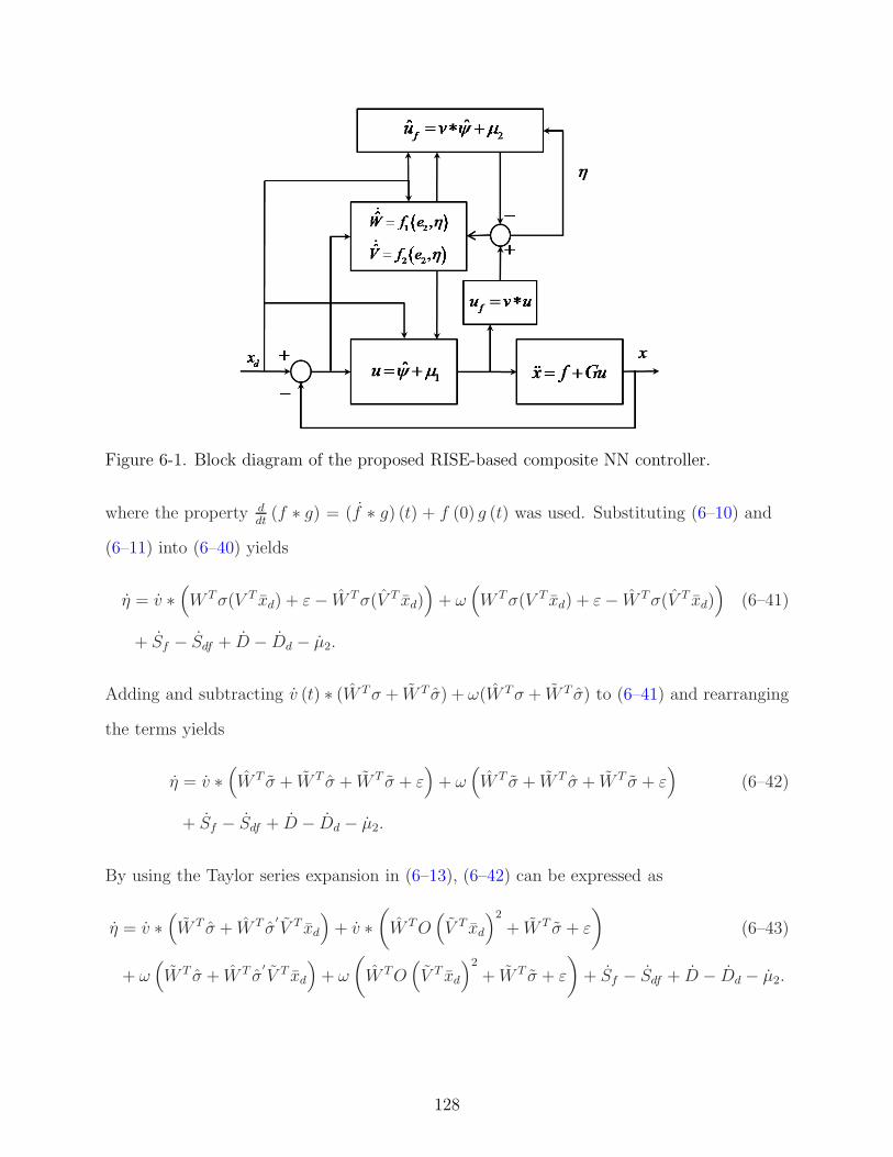
Figure 6-1. Block diagram of the proposed RISE-based composite NN controller.

where the property ddt

(f ∗ g) = (f ∗ g) (t) + f (0) g (t) was used. Substituting (6–10) and

(6–11) into (6–40) yields

η = v ∗(

W Tσ(V T xd) + ε− W Tσ(V T xd))

+ ω(

W Tσ(V T xd) + ε− W Tσ(V T xd))

(6–41)

+ Sf − Sdf + D − Dd − µ2.

Adding and subtracting v (t) ∗ (W Tσ + W T σ) + ω(W Tσ + W T σ) to (6–41) and rearranging

the terms yields

η = v ∗(

W T σ + W T σ + W T σ + ε)

+ ω(

W T σ + W T σ + W T σ + ε)

(6–42)

+ Sf − Sdf + D − Dd − µ2.

By using the Taylor series expansion in (6–13), (6–42) can be expressed as

η = v ∗(

W T σ + W T σ′

V T xd

)

+ v ∗

(

W TO(

V T xd

)2

+ W T σ + ε

)

(6–43)

+ ω(

W T σ + W T σ′

V T xd

)

+ ω

(

W TO(

V T xd

)2

+ W T σ + ε

)

+ Sf − Sdf + D − Dd − µ2.

128

Using the commutativity and distributivity property of the convolution, and rearranging

the terms in (6–43) yields

η = W T (σ ∗ v + ωσ) + W T σ′

V T (xd ∗ v + ωxd) + N2 +N2B − k2η − β2sgn(η) (6–44)

where the fact that

µ2 = k2η + β2sgn(η) (6–45)

was utilized. In (6–44), the unmeasurable/unknown auxiliary term N2(e1, e2, r, t) ∈ Rn is

defined as

N2 , Sf − Sdf (6–46)

and the term N2B (t) ∈ Rn is defined as

N2B , D − Dd + v ∗

(

W TO(

V T xd

)2

+ W T σ + ε

)

+ ω

(

W TO(

V T xd

)2

+ W T σ + ε

)

.

(6–47)

In a similar manner as in Lemma 1 of the Appendix, by applying the Mean Value

Theorem can be used to develop the following upper bound for the expression in (6–46):

∥

∥

∥N2(t)

∥

∥

∥≤ ρ2 (‖z‖) ‖z‖ (6–48)

where the bounding function ρ2(·) ∈ R is a positive, globally invertible, nondecreasing

function, and z(t) ∈ R3n is defined as

z(t) ,[

eT1 eT

2 rT]T. (6–49)

Using Assumption 6-3, and the fact that v (t) is a linear, strictly proper, exponentially

stable transfer function, the following inequality can be developed based on the expression

in (6–47) with a similar approach as in Lemma 2 of [42]:

‖N2B(t)‖ ≤ ξ (6–50)

where ξ ∈ R is a known positive constant.

129

6.4.2 Composite Adaptation

The composite adaptation for the NN weight estimates is given by

·

W , Γ1proj(α2σ′

V T·

xdeT2 +

·

σfηT ) (6–51)

·

V , Γ2proj(α2

·

xdeT2 W

T σ′

+·

xdfηT W T σ

′

) (6–52)

where Γ1 ∈ R(N2+1)×(N2+1), Γ2 ∈ R(N1+1)×(N1+1) are constant, positive definite, symmetric

control gain matrices, proj (·) denotes a smooth projection operator (see [70, 75]) that

is used to ensure that W (t) and V (t) remain inside the bounded convex region. Also,

η (t) ∈ Rn denotes the measurable prediction error defined in (6–20), and the scalar

function v (t) was defined in (6–23). The filtered activation function σf (t) ∈ RN2+1 is

generated from the stable first order differential equation

·

σf + ωσf = ωσ, σf (0) = 0 (6–53)

while the filtered NN input vector xdf (t) ∈ R3n+1 is generated by

·

xdf + ωxdf = ωxd, xdf (0) = 0. (6–54)

In a typical NN weight adaptation law, only the system tracking errors are used

to update the weights and no information about the actual estimate mismatch (i.e.,

ψ (t) − ψ (t)) is utilized as it is unmeasurable, and hence cannot be used in control

implementation. The proposed method uses the swapping procedure in Section 6.4.1

to generate a measurable prediction error η (t) that contains information related to the

estimate mismatch error.

130

The projection used in the NN weight adaptation laws in (6–51) and (6–52) can be

decomposed into two terms as1

·

W = χWη + χW

e2,

·

V = χVη + χV

e2(6–55)

such that the auxiliary functions χWη (σf , η) , χ

We2

(

V , xd,·

xd, e2

)

∈ R(N2+1)×n and

χVη

(

xdf , W , V , η)

, χVe2

(

W , V , xd,·

xd, e2

)

∈ R(N1+1)×N2 satisfy the following bounds

∥

∥χWη

∥

∥ ≤ b1 ‖η‖ ,∥

∥χWe2

∥

∥ ≤ b2 ‖e2‖ (6–56)

∥

∥χVη

∥

∥ ≤ b′

1 ‖η‖ ,∥

∥χVe2

∥

∥ ≤ b′

2 ‖e2‖

where b1, b2, b′

1, and b′

2 ∈ R are known positive constants. To facilitate the subsequent

stability analysis, the following inequality is developed based on (6–56) and the fact that

the NN weight estimates are bounded by the smooth projection algorithm:

∥

∥

∥χW

η σ + W T σ′

χVη xd

∥

∥

∥≤ c1 ‖η‖ (6–57)

where c1 ∈ R is a positive constant.

6.4.3 Closed-Loop Error System

Substituting for·

W (t) and·

V (t) from (6–55), the expression in (6–19) can be

rewritten as

G−1r = −1

2G−1r − χW

η σ − W T σ′

χVη xd + N1 +N1 − (k1 + 1)r − β1sgn(e2) − e2 (6–58)

where the fact that the time derivative of (6–16) is given as

µ1 = (k1 + 1)r + β1sgn(e2) (6–59)

1 See Lemma 5 of the Appendix for the proof of the decomposition in (6–55) and theinequalities in (6–56).

131

was utilized. In (6–58), the unmeasurable/unknown auxiliary terms N1(e1, e2, r, t) and

N1 (t) ∈ Rn are defined as

N1 , −1

2G−1r + S1 + e2 − χW

e2σ − W T σ

′

χVe2xd (6–60)

N1 , Nd +N1B. (6–61)

In (6–61), Nd(xd,·

xd, t) ∈ Rn is defined as

Nd , W Tσ′

V T·

xd + ε (6–62)

while N1B(W , V , xd,·

xd, t) ∈ Rn is further segregated as

N1B , N1Ba+N1Bb

(6–63)

where N1Ba(W , V , xd,

·

xd, t) ∈ Rn is defined as

N1Ba, −W T σ

′

V T·

xd − W T σ′

V T·

xd (6–64)

and the term N1Bb(W , V , xd,

·

xd, t) ∈ Rn is defined as

N1Bb, W T σ

′

V T·

xd + W T σ′

V T·

xd. (6–65)

Motivation for segregating the terms in (6–61) is derived from the fact that the different

components in (6–61) have different bounds. Segregating the terms as in (6–61)-(6–65)

facilitates the development of the NN weight update laws and the subsequent stability

analysis. For example, the terms in (6–62) are grouped together because the terms and

their time derivatives can be upper bounded by a constant and rejected by the RISE

feedback, whereas the terms grouped in (6–63) can be upper bounded by a constant but

their derivatives are state dependent. The state dependency of the time derivatives of

the terms in (6–63) violates the assumptions given in previous RISE-based controllers

(e.g., [19, 20, 22, 23, 25–27]), and requires additional consideration in the adaptation

law design and stability analysis. The terms in (6–63) are further segregated because

132

N1Ba(W , V , xd,

·

xd) will be rejected by the RISE feedback, whereas N1Bb(W , V , xd,

·

xd) will

be partially rejected by the RISE feedback and partially canceled by the adaptive update

law for the NN weight estimates. In a similar manner as in (6–48), the following upper

bound is developed for the expression in (6–60):

∥

∥

∥N1(t)

∥

∥

∥≤ ρ1 (‖z‖) ‖z‖ (6–66)

where the bounding function ρ1(·) ∈ R is a positive, globally invertible, nondecreasing

function, and z(t) ∈ R3n was defined in (6–49). The following inequalities can be

developed based on Assumption 6-3, (3–7), (3–8), (3–16), (6–63)-(6–65):

‖Nd‖ ≤ ζ1, ‖N1Ba‖ ≤ ζ2, ‖N1Bb

‖ ≤ ζ3,∥

∥

∥Nd

∥

∥

∥≤ ζ4. (6–67)

From (6–61), (6–63) and (6–67), the following bound can be developed

‖N1‖ ≤ ‖Nd‖ + ‖N1B‖ ≤ ‖Nd‖ + ‖N1Ba‖ + ‖N1Bb

‖ ≤ ζ1 + ζ2 + ζ3. (6–68)

By using (6–51) and (6–52), the time derivative of N1B(W , V , xd) can be bounded as

∥

∥

∥N1B

∥

∥

∥≤ ζ5 + ζ6 ‖e2‖ + ζ7 ‖η‖ . (6–69)

In (6–67) and (6–69), ζi ∈ R, (i = 1, 2, ..., 7) are known positive constants.

For the subsequent stability analysis, let D ⊂ R4n+3 be a domain containing y(t) = 0,

where y(t) ∈ R4n+3 is defined as

y , [zT ηT√

P1

√

P2

√

Q]T . (6–70)

In (6–70), the auxiliary function P1(t) ∈ R is defined as

P1 (t) , β1

n∑

i=1

|e2i(0)| − e2(0)TN1(0) −

∫ t

0

L1(τ)dτ (6–71)

133

where e2i (0) ∈ R denotes the ith element of the vector e2 (0), and the auxiliary function

L1(t) ∈ R is defined as

L1 , rT (N1Ba+Nd − β1sgn(e2)) + eT

2N1Bb− β3 ‖e2‖

2 − β4 ‖η‖2 (6–72)

where β1, β3, β4 ∈ R are positive constants chosen according to the sufficient conditions

β1 > max

ζ1 + ζ2 + ζ3, ζ1 + ζ2 +ζ4α2

+ζ5α2

, β3 > ζ6 +ζ72

, β4 >ζ72

(6–73)

where ζ1 − ζ7 were introduced in (6–67) and (6–69). Provided the sufficient conditions

introduced in (6–73) are satisfied, the following inequality is obtained [22], [20]:

∫ t

0

L1(τ)dτ ≤ β1

n∑

i=1

|e2i(0)| − e2(0)TN1(0). (6–74)

Hence, (6–74) can be used to conclude that P1(t) ≥ 0. Also in (6–70), the auxiliary

function P2(t) ∈ R is defined as

P2 (t) , −

∫ t

0

L2(τ)dτ (6–75)

where the auxiliary function L2(t) ∈ R is defined as

L2 , ηT (N2B − β2sgn(η)) (6–76)

where β2 ∈ R is a positive constant chosen according to the sufficient condition

β2 > ξ (6–77)

where ξ was introduced in (6–50). Provided the sufficient condition introduced in (6–77) is

satisfied, then P2(t) ≥ 0. The auxiliary function Q(t) ∈ R in (6–70) is defined as

Q(t) ,1

2tr(

W TΓ−11 W

)

+1

2tr(

V T Γ−12 V

)

. (6–78)

Since Γ1 and Γ2 are constant, symmetric, and positive definite matrices, it is straightforward

that Q(t) ≥ 0.

134

6.5 Stability Analysis

Theorem 6-1: The controller given in (6–15) and (6–16) in conjunction with

the composite NN adaptation laws in (6–51) and (6–52), where the prediction error

is generated from (6–20), (6–21), (6–37), and (6–38), ensures that all system signals

are bounded under closed-loop operation and that the position tracking error and the

prediction error are regulated in the sense that

‖e1(t)‖ → 0 and ‖η(t)‖ → 0 as t→ ∞

provided the control gains k1 and k2 introduced in (6–16) and (6–38) are selected

sufficiently large based on the initial conditions of the systems states (see the subsequent

semi-global stability proof), the sufficient conditions in (6–73) and (6–77) are satisfied, and

the following conditions are satisfied:

α1 >1

2, α2 > β3 +

1

2(6–79)

where the gains α1 and α2 were introduced in (6–4) and (6–5).

Proof: Let VL(y, t) : D× [0,∞) → R be a continuously differentiable, positive definite

function defined as

VL ,1

2eT1 e1 +

1

2eT2 e2 +

1

2rTG−1r +

1

2ηTη + P1 + P2 +Q (6–80)

which satisfies the inequalities

U1(y) ≤ VL(y, t) ≤ U2(y) (6–81)

provided the sufficient conditions introduced in (6–73) and (6–77) are satisfied. In (6–81),

the continuous positive definite functions U1(y), U2(y) ∈ R are defined as U1(y) , λ1 ‖y‖2

135

and U2(y) , λ2(x) ‖y‖2, where λ1, λ2(x) ∈ R are defined as

λ1 ,1

2min

1, g

(6–82)

λ2 , max1

2g(x), 1

where g, g(x) are introduced in (6–2). Using (6–4), (6–5), (6–44), (6–58), (6–71), (6–72),

(6–75) and (6–76), the time derivative of (6–80) can be expressed as

VL = eT1 (e2 − α1e1) + eT

2 (r − α2e2) + rT (−1

2G−1r − χW

η σ − W T σ′

χVη xd + N1 (6–83)

+N1 − (k1 + 1)r − β1sgn(e2) − e2) +1

2rT G−1r + ηT (W T

·

σf + W T σ′

V T·

xdf

+ N2 +N2B − k2η − β2sgn(η)) − rT (N1Ba+Nd − β1sgn(e2)) − eT

2N1Bb

+ β3 ‖e2‖2 + β4 ‖η‖

2 − ηT (N2B − β2sgn(η)) − tr(W TΓ−11

·

W ) − tr(V T Γ−12

·

V ).

Expanding the terms in (6–83) and using (6–61) and (6–63) yields

VL = eT1 e2 − α1e

T1 e1 + eT

2 r − α2eT2 e2 + rT N1 −

1

2rT G−1r − rTχW

η σ − rTW T σ′

χVη xd (6–84)

+ rT (Nd +N1Ba) + (e2 + α2e2)

T N1Bb− (k1 + 1)rTr − β1r

T sgn(e2) − rT e2

+ ηT W T·

σf + ηTW T σ′

V T·

xdf − ηTN2B + ηT N2 + ηTN2B − k2ηTη − β2η

T sgn(η)

− rT (N1Ba+Nd − β1sgn(e2)) − e2(t)

TN1Bb+ β3 ‖e2‖

2 + β4 ‖η‖2 + β2η

T sgn(η))

+1

2rT G−1r − tr(W TΓ−1

1

·

W ) − tr(V T Γ−12

·

V ).

Canceling the common terms in (6–84), and substituting for N1Bbfrom (6–65), and using

the fact that aT b = tr(

baT)

, VL(y, t) is expressed as

VL = eT1 e2 − α1e

T1 e1 − α2e

T2 e2 − k2η

Tη − rTχWη σ − rT W T σ

′

χVη xd + rT N1 (6–85)

− (k1 + 1)rT r + β3 ‖e2‖2 + β4 ‖η‖

2 + ηT N2 + tr(

α2WT σ

′

V T·

xdeT2

)

+ tr

(

W T·

σfηT

)

+ tr(

α2VT

·

xd(σ′T W e2)

T)

+ tr

(

V T·

xdf

(

σ′T Wη

)T)

− tr(W T Γ−11

·

W ) − tr(V T Γ−12

·

V ).

136

Substituting the update laws from (6–51) and (6–52) in (6–85), canceling the similar

terms, and using the fact that eT1 e2 ≤ 1

2(‖e1‖

2 + ‖e2‖2), the expression in (6–85) is upper

bounded as

VL ≤ −

(

α1 −1

2

)

‖e1‖2 −

(

α2 −1

2− β3

)

‖e2‖2 − ‖r‖2 + c1 ‖η‖ ‖r‖ + ‖r‖

∥

∥

∥N1

∥

∥

∥− k1 ‖r‖

2

+ ‖η‖∥

∥

∥N2

∥

∥

∥− (k2 − β4) ‖η‖

2

where (6–57) was used. Using the squares of the components of z(t), VL(y, t) is upper

bounded as

VL ≤ −λ3 ‖z‖2 − k1 ‖r‖

2 + ‖r‖∥

∥

∥N1

∥

∥

∥+ c1 ‖η‖ ‖z‖ + ‖η‖

∥

∥

∥N2

∥

∥

∥− k2 ‖η‖

2 (6–86)

where

λ3 , minα1 −1

2, α2 −

1

2− β3, 1.

Letting

k2 = k2a + k2b

where k2a, k2b ∈ R are positive constants, and using the inequalities in (6–48) and (6–66),

the expression in (6–86) is upper bounded as

VL ≤ −λ3 ‖z‖2 − (k2b − β4) ‖η‖

2 −[

k1 ‖r‖2 − ρ1(‖z‖) ‖r‖ ‖z‖

]

(6–87)

−[

k2a ‖η‖2 − (ρ2(‖z‖) + c1) ‖η‖ ‖z‖

]

.

Completing the squares for the terms inside the brackets in (6–87) yields

VL ≤ −λ3 ‖z‖2 − (k2b − β4) ‖η‖

2 +ρ2

1(‖z‖) ‖z‖2

4k1+

(ρ2(‖z‖) + c1)2 ‖z‖2

4k2a

≤ −λ3 ‖z‖2 +

ρ2(‖z‖) ‖z‖2

4k− (k2b − β4) ‖η‖

2 (6–88)

where k ∈ R is defined as

k , min k1, k2a (6–89)

137

and ρ(·) ∈ R is a positive, globally invertible, nondecreasing function defined as

ρ2(‖z‖) , ρ21(‖z‖) + (ρ2(‖z‖) + c1)

2 .

The expression in (6–88) can be further upper bounded by a continuous, positive

semi-definite function

VL(y, t) ≤ −U(y) = −c∥

∥

∥

[

zT ηT]T∥

∥

∥

2

∀y ∈ D (6–90)

for some positive constant c ∈ R, where

D ,

y (t) ∈ R4n+3 | ‖y‖ ≤ ρ−1

(

2√

λ3k)

.

Larger values of k will expand the size of the domain D. The inequalities in (6–81)

and (6–90) can be used to show that VL(y, t) ∈ L∞ in D; hence, e1(t), e2(t), r(t), and

η (t) ∈ L∞ in D. Given that e1(t), e2(t), and r(t) ∈ L∞ in D, standard linear analysis

methods can be used to prove that e1(t), and e2(t) ∈ L∞ in D from (6–4) and (6–5). Since

e1(t), e2(t), and r(t) ∈ L∞ in D, Assumption 6-3 can be used along with (6–3)-(6–5) to

conclude that x(i)(t) ∈ L∞, in D. Since x(i)(t) ∈ L∞, in D, Assumption 6-2 can be used to

conclude that G−1(·) and f(·) ∈ L∞ in D. Thus, from (6–1) we can show that u(t) ∈ L∞

in D. Therefore, uf(t) ∈ L∞ in D, and hence, from (6–20), uf(t) ∈ L∞ in D. Given that

r(t) ∈ L∞ in D, (6–59) can be used to show that µ1(t) ∈ L∞ in D, and since G−1(·) and

f(·) ∈ L∞ in D, (6–58) can be used to show that r(t) ∈ L∞ in D, and (6–44) can be used

to show that η(t) ∈ L∞ in D. Since e1(t), e2(t), r(t), and η (t) ∈ L∞ in D, the definitions

for U(y) and z(t) can be used to prove that U(y) is uniformly continuous in D.

Let S ⊂ D denote a set defined as

S ,

y(t) ∈ D | U2(y(t)) < λ1

(

ρ−1(

2√

λ3k))2

. (6–91)

The region of attraction in (6–91) can be made arbitrarily large to include any initial

conditions by increasing the control gain k (i.e., a semi-global stability result). Theorem

138

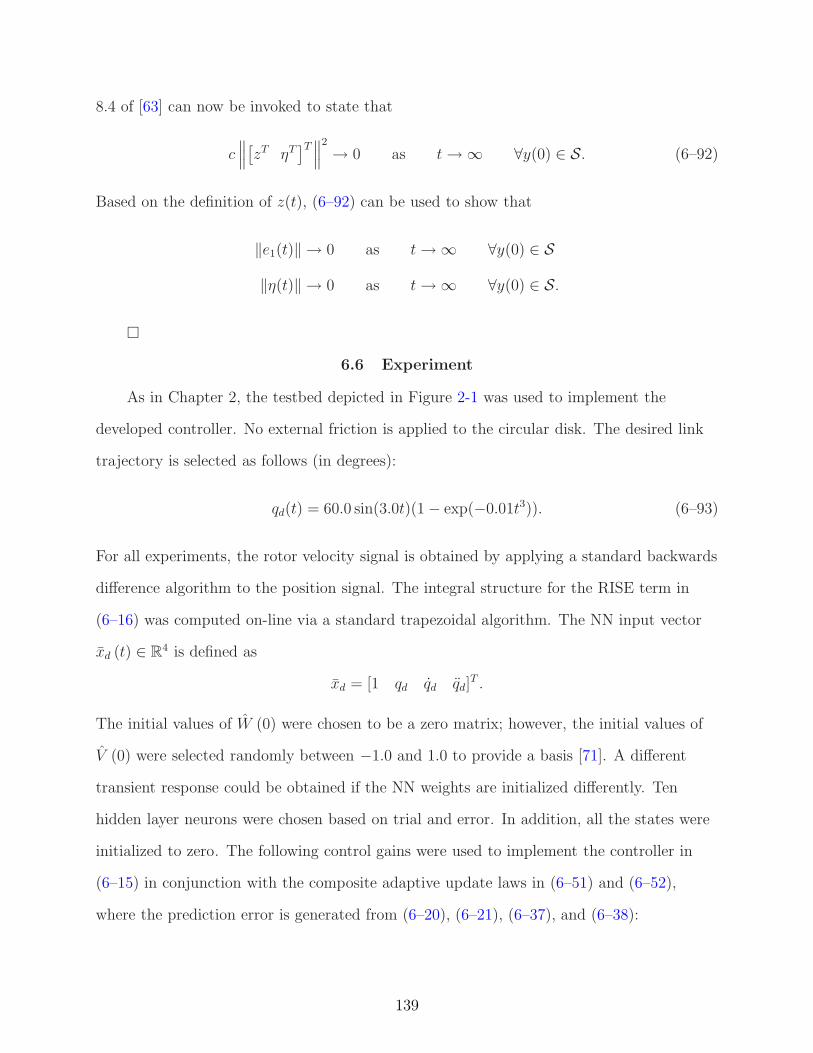
8.4 of [63] can now be invoked to state that

c∥

∥

∥

[

zT ηT]T∥

∥

∥

2

→ 0 as t→ ∞ ∀y(0) ∈ S. (6–92)

Based on the definition of z(t), (6–92) can be used to show that

‖e1(t)‖ → 0 as t→ ∞ ∀y(0) ∈ S

‖η(t)‖ → 0 as t→ ∞ ∀y(0) ∈ S.

6.6 Experiment

As in Chapter 2, the testbed depicted in Figure 2-1 was used to implement the

developed controller. No external friction is applied to the circular disk. The desired link

trajectory is selected as follows (in degrees):

qd(t) = 60.0 sin(3.0t)(1 − exp(−0.01t3)). (6–93)

For all experiments, the rotor velocity signal is obtained by applying a standard backwards

difference algorithm to the position signal. The integral structure for the RISE term in

(6–16) was computed on-line via a standard trapezoidal algorithm. The NN input vector

xd (t) ∈ R4 is defined as

xd = [1 qd qd qd]T .

The initial values of W (0) were chosen to be a zero matrix; however, the initial values of

V (0) were selected randomly between −1.0 and 1.0 to provide a basis [71]. A different

transient response could be obtained if the NN weights are initialized differently. Ten

hidden layer neurons were chosen based on trial and error. In addition, all the states were

initialized to zero. The following control gains were used to implement the controller in

(6–15) in conjunction with the composite adaptive update laws in (6–51) and (6–52),

where the prediction error is generated from (6–20), (6–21), (6–37), and (6–38):

139

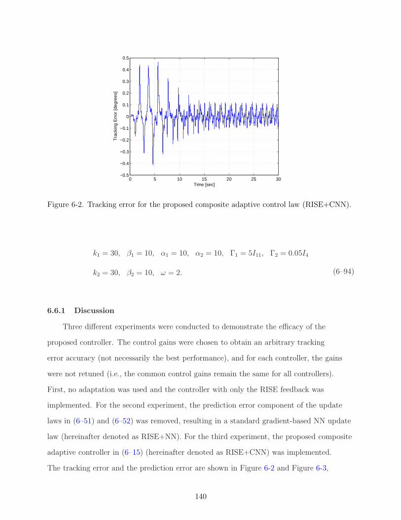
0 5 10 15 20 25 30−0.5

−0.4

−0.3

−0.2

−0.1

0

0.1

0.2

0.3

0.4

0.5

Tra

ckin

g E

rror

[deg

rees

]

Time [sec]

Figure 6-2. Tracking error for the proposed composite adaptive control law (RISE+CNN).

k1 = 30, β1 = 10, α1 = 10, α2 = 10, Γ1 = 5I11, Γ2 = 0.05I4

k2 = 30, β2 = 10, ω = 2. (6–94)

6.6.1 Discussion

Three different experiments were conducted to demonstrate the efficacy of the

proposed controller. The control gains were chosen to obtain an arbitrary tracking

error accuracy (not necessarily the best performance), and for each controller, the gains

were not retuned (i.e., the common control gains remain the same for all controllers).

First, no adaptation was used and the controller with only the RISE feedback was

implemented. For the second experiment, the prediction error component of the update

laws in (6–51) and (6–52) was removed, resulting in a standard gradient-based NN update

law (hereinafter denoted as RISE+NN). For the third experiment, the proposed composite

adaptive controller in (6–15) (hereinafter denoted as RISE+CNN) was implemented.

The tracking error and the prediction error are shown in Figure 6-2 and Figure 6-3,

140

0 5 10 15 20 25 30−0.2

−0.15

−0.1

−0.05

0

0.05

0.1

0.15

0.2

Pre

dict

ion

Err

or [N

−m

]

Time [sec]

Figure 6-3. Prediction error for the proposed composite adaptive control law(RISE+CNN).

0 5 10 15 20 25 30

−15

−10

−5

0

5

10

15

Tor

que

[N−

m]

Time [sec]

Figure 6-4. Control torque for the proposed composite adaptive control law (RISE+CNN).

141

Figure 6-5. Average RMS errors (degrees) and torques (N-m). 1- RISE, 2- RISE+NN, 3-RISE+CNN (proposed).

respectively. The control torque is shown in Figure 6-4. Each experiment was performed

five times and the average RMS error and torque values are shown in Figure 6-5, which

indicate that the proposed RISE+CNN controller yields the lowest RMS error with a

similar control effort.

6.7 Conclusion

A first ever gradient-based composite NN controller is developed for nonlinear

uncertain systems. A NN feedforward component is used in conjunction with the RISE

feedback, where the NN weight estimates are generated using a composite update law

driven by both the tracking and the prediction error with the motivation of using

more information in the NN update law. The construction of a NN-based controller to

approximate the unknown system dynamics inherently results in a residual function

reconstruction error. The presence of the reconstruction error has been the technical

obstacle that has prevented the development of composite adaptation laws for NNs.

To compensate for the effects of the reconstruction error, the typical prediction error

formulation is modified to include a RISE-like structure in the design of the estimated

filtered control input. Using a Lyapunov stability analysis, sufficient gain conditions

are derived under which the proposed controller yields semi-global asymptotic stability.

142

Experiments on a rotating disk indicate that the proposed method yields better tracking

performance with a similar control effort.

143

CHAPTER 7CONCLUSIONS AND FUTURE WORK

7.1 Conclusions

A new class of asymptotic controllers is developed that contains an adaptive

feedforward term to account for linear parameterizable uncertainty and a high gain RISE

feedback term which accounts for unstructured disturbances. In comparison with previous

results that used a similar high gain feedback control structure, new control development

was required to include the additional adaptive feedforward term. The motivation for

injecting the adaptive feedforward term is that improved tracking performance and

reduced control effort result from including more knowledge of the system dynamics in the

control structure. This heuristic idea was verified by our experimental results that indicate

reduced control effort and reduced RMS tracking errors.

The research further illustrates how a multilayer NN feedforward term can be fused

with a RISE feedback term in a continuous controller to achieve semi-global asymptotic

tracking. Improved weight tuning laws are presented which guarantee boundedness of NN

weights. To blend the NN and RISE methods, several technical challenges were addressed

through Lyapunov-based techniques. These challenges include developing adaptive update

laws for the NN weight estimates that do not depend on acceleration, and developing

new RISE stability analysis methods and sufficient gain conditions to accommodate the

incorporation of the NN adaptive updates in the RISE structure. Experimental results are

presented that indicate reduced RMS tracking errors.

Further, a RISE-based approach was presented to achieve modularity in the

controller/update law for a general class of multi-input systems. Specifically, for systems

with structured and unstructured uncertainties, a controller was employed that uses a

model-based feedforward adaptive term in conjunction with the RISE feedback term.

The adaptive feedforward term was made modular by considering a generic form of

the adaptive update law and its corresponding parameter estimate. This generic form

144

of the update law was used to develop a new closed-loop error system, and the typical

RISE stability analysis was modified. New sufficient gain conditions were derived to

show asymptotic tracking of the desired link position. The class of RISE-based modular

adaptive controllers is then extended to include uncertain dynamic systems that do not

satisfy the LP assumption. Specifically, the result allows the NN weight tuning laws

to be determined from a developed generic update law (rather than being restricted to

a gradient update law). The modular adaptive control development is then applied to

Euler-Lagrange dynamic systems. An experimental section is included that illustrates the

concept.

In addition, a novel approach for the design of a gradient-based composite adaptive

controller was proposed for generic MIMO systems subjected to bounded disturbances.

A model-based feedforward adaptive component was used in conjunction with the RISE

feedback, where the adaptive estimates were generated using a composite update law

driven by both the tracking and prediction error with the motivation of using more

information in the adaptive update law. To account for the effects of non-LP disturbances,

the typical prediction error formulation was modified to include a second RISE-like term

in the estimated filtered control input design. Using a Lyapunov stability analysis,

sufficient gain conditions were derived under which the proposed controller yields

semi-global asymptotic stability. Experiments on a rotating disk with externally applied

friction indicate that the proposed method yields better tracking performance with a

similar control effort.

This technique is then extended to develop a first ever gradient-based composite

NN controller for nonlinear uncertain systems. A NN feedforward component is used

in conjunction with the RISE feedback, where the NN weight estimates are generated

using a composite update law driven by both the tracking and the prediction error with

the motivation of using more information in the NN update law. The construction of a

NN-based controller to approximate the unknown system dynamics inherently results

145

in a residual function reconstruction error. The presence of the reconstruction error has

been the technical obstacle that has prevented the development of composite adaptation

laws for NNs. To compensate for the effects of the reconstruction error, the typical

prediction error formulation is modified to include a RISE-like structure in the design of

the estimated filtered control input. Using a Lyapunov stability analysis, sufficient gain

conditions are derived under which the proposed controller yields semi-global asymptotic

stability.

7.2 Future Work

• The results in this dissertation, as well as all previous RISE controllers, requirefull-state feedback. The development of an output feedback result remains an openproblem.

• Also, one of the shortcomings of current work is that only a semi-global asymptoticstability is achieved, and further investigation is needed to achieve a global stabilityresult. Inroads to solve the global tracking problem are provided in [78] under a setof assumptions.

• While the modular adaptive result in Chapter 4 encompasses a large variety ofadaptive update laws, an update law design based on the prediction error is notpossible because the formulation of a prediction error requires the system dynamicsto be completely LP. Future efforts can focus on developing a adaptive controllerthat could also use a prediction error in the modular adaptive update law.

• The composite adaptation presented in Chapters 5 and 6 utilize the gradient-basedupdate laws. Future efforts could focus on developing composite adaptation that useleast-squares estimation.

146

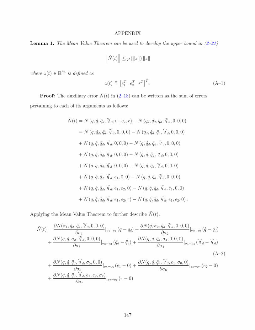
APPENDIX

Lemma 1. The Mean Value Theorem can be used to develop the upper bound in (2–21)

∥

∥

∥N(t)

∥

∥

∥≤ ρ (‖z‖) ‖z‖

where z(t) ∈ R3n is defined as

z(t) ,[

eT1 eT

2 rT]T. (A–1)

Proof: The auxiliary error N(t) in (2–18) can be written as the sum of errors

pertaining to each of its arguments as follows:

N(t) = N (q, q, qd,...q d, e1, e2, r) −N (qd, qd, qd,

...q d, 0, 0, 0)

= N (q, qd, qd,...q d, 0, 0, 0) −N (qd, qd, qd,

...q d, 0, 0, 0)

+N (q, q, qd,...q d, 0, 0, 0) −N (q, qd, qd,

...q d, 0, 0, 0)

+N (q, q, qd,...q d, 0, 0, 0) −N (q, q, qd,

...q d, 0, 0, 0)

+N (q, q, qd,...q d, 0, 0, 0) −N (q, q, qd,

...q d, 0, 0, 0)

+N (q, q, qd,...q d, e1, 0, 0) −N (q, q, qd,

...q d, 0, 0, 0)

+N (q, q, qd,...q d, e1, e2, 0) −N (q, q, qd,

...q d, e1, 0, 0)

+N (q, q, qd,...q d, e1, e2, r) −N (q, q, qd,

...q d, e1, e2, 0) .

Applying the Mean Value Theorem to further describe N(t),

N(t) =∂N(σ1, qd, qd,

...q d, 0, 0, 0)

∂σ1|σ1=v1 (q − qd) +

∂N(q, σ2, qd,...q d, 0, 0, 0)

∂σ2|σ2=v2 (q − qd)

+∂N(q, q, σ3,

...q d, 0, 0, 0)

∂σ3

|σ3=v3 (qd − qd) +∂N(q, q, qd, σ4, 0, 0, 0)

∂σ4

|σ4=v4 (...q d −

...q d)

(A–2)

+∂N(q, q, qd,

...q d, σ5, 0, 0)

∂σ5|σ5=v5 (e1 − 0) +

∂N(q, q, qd,...q d, e1, σ6, 0)

∂σ6|σ6=v6 (e2 − 0)

+∂N(q, q, qd,

...q d, e1, e2, σ7)

∂σ7|σ7=v7 (r − 0)

147

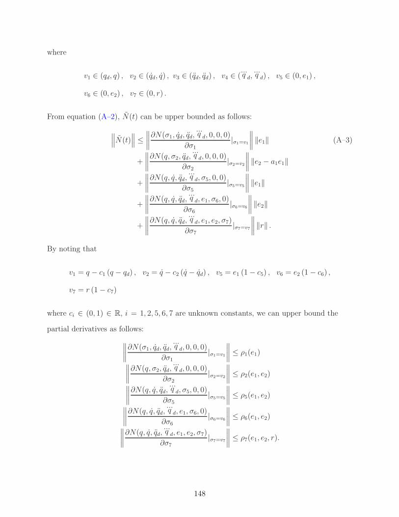
where

v1 ∈ (qd, q) , v2 ∈ (qd, q) , v3 ∈ (qd, qd) , v4 ∈ (...q d,

...q d) , v5 ∈ (0, e1) ,

v6 ∈ (0, e2) , v7 ∈ (0, r) .

From equation (A–2), N(t) can be upper bounded as follows:

∥

∥

∥N(t)

∥

∥

∥≤

∥

∥

∥

∥

∂N(σ1, qd, qd,...q d, 0, 0, 0)

∂σ1

|σ1=v1

∥

∥

∥

∥

‖e1‖ (A–3)

+

∥

∥

∥

∥

∂N(q, σ2, qd,...q d, 0, 0, 0)

∂σ2|σ2=v2

∥

∥

∥

∥

‖e2 − a1e1‖

+

∥

∥

∥

∥

∂N(q, q, qd,...q d, σ5, 0, 0)

∂σ5|σ5=v5

∥

∥

∥

∥

‖e1‖

+

∥

∥

∥

∥

∂N(q, q, qd,...q d, e1, σ6, 0)

∂σ6

|σ6=v6

∥

∥

∥

∥

‖e2‖

+

∥

∥

∥

∥

∂N(q, q, qd,...q d, e1, e2, σ7)

∂σ7|σ7=v7

∥

∥

∥

∥

‖r‖ .

By noting that

v1 = q − c1 (q − qd) , v2 = q − c2 (q − qd) , v5 = e1 (1 − c5) , v6 = e2 (1 − c6) ,

v7 = r (1 − c7)

where ci ∈ (0, 1) ∈ R, i = 1, 2, 5, 6, 7 are unknown constants, we can upper bound the

partial derivatives as follows:

∥

∥

∥

∥

∂N(σ1, qd, qd,...q d, 0, 0, 0)

∂σ1

|σ1=v1

∥

∥

∥

∥

≤ ρ1(e1)

∥

∥

∥

∥

∂N(q, σ2, qd,...q d, 0, 0, 0)

∂σ2|σ2=v2

∥

∥

∥

∥

≤ ρ2(e1, e2)

∥

∥

∥

∥

∂N(q, q, qd,...q d, σ5, 0, 0)

∂σ5|σ5=v5

∥

∥

∥

∥

≤ ρ5(e1, e2)

∥

∥

∥

∥

∂N(q, q, qd,...q d, e1, σ6, 0)

∂σ6

|σ6=v6

∥

∥

∥

∥

≤ ρ6(e1, e2)

∥

∥

∥

∥

∂N(q, q, qd,...q d, e1, e2, σ7)

∂σ7|σ7=v7

∥

∥

∥

∥

≤ ρ7(e1, e2, r).

148

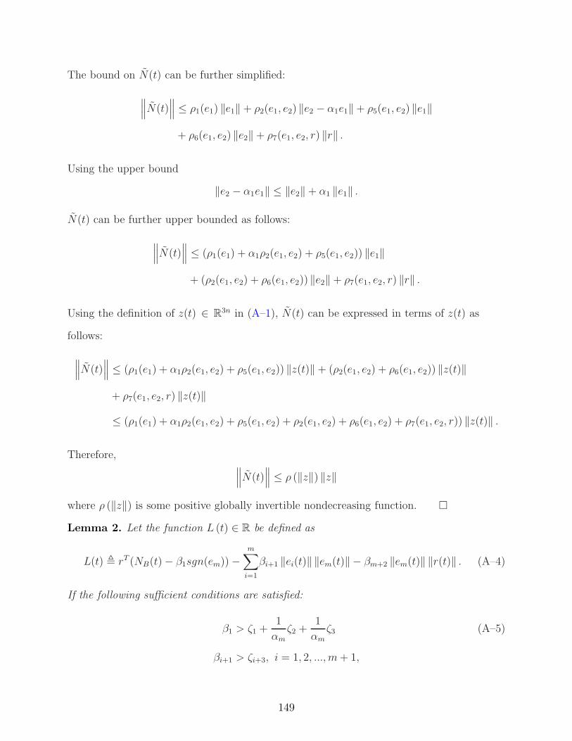
The bound on N(t) can be further simplified:

∥

∥

∥N(t)

∥

∥

∥≤ ρ1(e1) ‖e1‖ + ρ2(e1, e2) ‖e2 − α1e1‖ + ρ5(e1, e2) ‖e1‖

+ ρ6(e1, e2) ‖e2‖ + ρ7(e1, e2, r) ‖r‖ .

Using the upper bound

‖e2 − α1e1‖ ≤ ‖e2‖ + α1 ‖e1‖ .

N(t) can be further upper bounded as follows:

∥

∥

∥N(t)

∥

∥

∥≤ (ρ1(e1) + α1ρ2(e1, e2) + ρ5(e1, e2)) ‖e1‖

+ (ρ2(e1, e2) + ρ6(e1, e2)) ‖e2‖ + ρ7(e1, e2, r) ‖r‖ .

Using the definition of z(t) ∈ R3n in (A–1), N(t) can be expressed in terms of z(t) as

follows:

∥

∥

∥N(t)

∥

∥

∥≤ (ρ1(e1) + α1ρ2(e1, e2) + ρ5(e1, e2)) ‖z(t)‖ + (ρ2(e1, e2) + ρ6(e1, e2)) ‖z(t)‖

+ ρ7(e1, e2, r) ‖z(t)‖

≤ (ρ1(e1) + α1ρ2(e1, e2) + ρ5(e1, e2) + ρ2(e1, e2) + ρ6(e1, e2) + ρ7(e1, e2, r)) ‖z(t)‖ .

Therefore,∥

∥

∥N(t)

∥

∥

∥≤ ρ (‖z‖) ‖z‖

where ρ (‖z‖) is some positive globally invertible nondecreasing function.

Lemma 2. Let the function L (t) ∈ R be defined as

L(t) , rT (NB(t) − β1sgn(em)) −m∑

i=1

βi+1 ‖ei(t)‖ ‖em(t)‖ − βm+2 ‖em(t)‖ ‖r(t)‖ . (A–4)

If the following sufficient conditions are satisfied:

β1 > ζ1 +1

αm

ζ2 +1

αm

ζ3 (A–5)

βi+1 > ζi+3, i = 1, 2, ..., m+ 1,

149

then∫ t

0

L(τ)dτ ≤ β1

n∑

i=1

|emi(0)| − em(0)TNB(0). (A–6)

Proof: Integrating both sides of the equation in (A–6)

∫ t

0

L(τ)dτ =

∫ t

0

(r(τ)T (NB(τ) − β1sgn(em(τ)) −

m∑

i=1

βi+1 ‖ei(τ)‖ ‖em(τ)‖ (A–7)

− βm+2 ‖em(τ)‖ ‖r(τ)‖)dτ.

Substituting (4–6) into (A–7),

∫ t

0

L(τ)dτ =

∫ t

0

dem(τ)

dτ

T

NB(τ)dτ +

∫ t

0

αmem(τ)T (NB(τ) − β1sgn(em(τ)))dτ

−

∫ t

0

dem(τ)

dτ

T

β1sgn(em(τ))dτ −

∫ t

0

m∑

i=1

βi+1 ‖ei(τ)‖ ‖em(τ)‖ dτ (A–8)

−

∫ t

0

βm+2 ‖em(τ)‖ ‖r(τ)‖ dτ.

Integrating the first integral in (A–8) by parts yields

∫ t

0

L(τ)dτ = em(τ)TNB(τ)∣

∣

t

0−

∫ t

0

em(τ)T dNB(τ)

dτdτ (A–9)

+

∫ t

0

αmem(τ)T (NB(τ) − β1sgn(em(τ)))dτ

−

∫ t

0

dem(τ)

dτ

T

β1sgn(em(τ))dτ −

∫ t

0

m∑

i=1

βi+1 ‖ei(τ)‖ ‖em(τ)‖ dτ

−

∫ t

0

βm+2 ‖em(τ)‖ ‖r(τ)‖ dτ.

By using the fact that

dNB(τ)

dτ=d (NB1(τ) +NB2(τ))

dτ=dNB1(τ)

dτ+dNB2(τ)

dτ,

150

the expression in (A–9) is rewritten as

∫ t

0

L(τ)dτ =

∫ t

0

αmem(τ)T (NB(τ) −1

αm

dNB1(τ)

dτ− β1sgn(em(τ)))dτ (A–10)

−

∫ t

0

em(τ)T dNB2(τ)

dτdτ −

∫ t

0

m∑

i=1

βi+1 ‖ei(τ)‖ ‖em(τ)‖ dτ

−

∫ t

0

βm+2 ‖em(τ)‖ ‖r(τ)‖ dτ − β1

n∑

i=1

|emi(t)| + β1

n∑

i=1

|emi(0)|

+em(t)TNB(t) − em(0)TNB(0).

Rearranging terms in (A–10), yields

∫ t

0

L(τ)dτ ≤

∫ t

0

αm ‖em(τ)‖ (‖NB(τ)‖ +1

αm

∥

∥

∥

∥

dNB1(τ)

dτ

∥

∥

∥

∥

− β1)dτ

+

∫ t

0

‖em(τ)‖

∥

∥

∥

∥

dNB2(τ)

dτ

∥

∥

∥

∥

dτ −

∫ t

0

m∑

i=1

βi+1 ‖ei(τ)‖ ‖em(τ)‖ dτ −

∫ t

0

βm+2 ‖em(τ)‖ ‖r(τ)‖ dτ

(A–11)

−β1 ‖em(t)‖ + β1

n∑

i=1

|emi(0)| + ‖em(t)‖ ‖NB(t)‖ − em(0)TNB(0)

where the fact thatn∑

i=1

|emi(t)| ≥ ‖em(t)‖

was used. Using the inequalities (4–31) in (A–11) yields

∫ t

0

L(τ)dτ ≤

∫ t

0

αm ‖em(τ)‖ (ζ1 +1

αm

ζ2 +1

αm

ζ3 − β1)dτ (A–12)

+

∫ t

0

‖em(τ)‖ (m∑

i=1

‖ei(τ)‖ (ζi+3 − βi+1))dτ +

∫ t

0

‖em(τ)‖ ‖r(τ)‖ (ζm+4 − βm+2)dτ

+ ‖em(t)‖ (ζ1 − β1) + β1

n∑

i=1

|emi(0)| − em(0)TNB(0).

From (A–12), if the sufficient conditions in (A–5) are satisfied, then (A–6) holds.

Lemma 3. The regions ΛV and ΛW defined in (3–9) and (3–11), respectively, are convex

[83].

151

Proof: Let vec (V1) and vec (V2) ∈ ΛV , therefore vec (V1)T vec (V1) ≤ VB and

vec (V2)T vec (V2) ≤ VB.

Consider

vec (V ) = λvec (V1) + (1 − λ) vec (V2) , λ ∈ [0, 1] . (A–13)

Taking the transpose of (A–13) and multiplying by itself yields

vec (V )T vec (V ) = λ2vec (V1)T vec (V1) + (1 − λ)2 vec (V2)

T vec (V2)

+ 2λ (1 − λ) vec (V1)T vec (V2) .

Using (3–7), the following inequality can be developed:

vec (V )T vec (V ) ≤ λ2VB + (1 − λ)2 VB + 2λ (1 − λ) VB

≤ VB.

Therefore, ΛV is convex. The convexity of ΛW follows the same development.

Lemma 4. Given the composite NN and RISE controller in (3–17)-(3–21), if vec(W (0)) ∈

int (ΛW ) and vec(V (0)) ∈ int (ΛV ), then W (t) and V (t) never leave the regions ΛW and

ΛV described in Assumption 3-2, respectively, and an upper bound for the expression given

in (3–51) can be formulated as follows

VL(y, t) ≤ rT N(t) − (ks + 1) ‖r‖2 (A–14)

− (2α1 − 1) ‖e1‖2 − (α2 − β2 − 1) ‖e2‖

2 .

Proof: The following nine cases must be considered (see Appendix B.3.2 of [70]).

Case 1: vec(W (t)) ∈ int (ΛW ), vec(V (t)) ∈ int (ΛV )

In this case, (3–51) can be expressed as

VL(y, t) = −2α1 ‖e1‖2 + 2eT

2 e1 + rT N(t) − (ks + 1) ‖r‖2 − α2 ‖e2‖2 + β2 ‖e2‖

2 (A–15)

+ α2eT2

[

W T (σ) + W T σ′

V Txd

]

− tr(α2WT σeT

2 ) − tr(α2VTxd(σ

′T We2)T ),

152

Based on the fact that

aT b = tr(

baT)

∀ a, b ∈ Rn

(A–15) can be reduced to (A–14). In addition, the direction in which the estimates

vec(W ) and vec(V ) are updated for Case 1 is irrelevant, since the worst case scenario is

that vec(W ) and vec(V ) will move towards the boundaries of the convex regions denoted

by ∂ (ΛW ) and ∂ (ΛV ), respectively, which is addressed subsequently.

Case 2: vec(W (t)) ∈ int (ΛW ),

vec(V ) ∈ ∂ (ΛV ) and vec (µ2)T vec(V )⊥ ≤ 0

In this case, (3–51) can be expressed as (A–15), which can be reduced to (A–14).

In addition, the vector vec (µ2) has a zero or nonzero component perpendicular to

the boundary ∂ (ΛV ) at vec(V ) that points in the direction towards the int (ΛV ).

Geometrically, this means that vec(V ) is updated such that it either moves towards

the int (ΛV ) or remains on the boundary. Hence, vec(V ) never leaves ΛV .

Case 3: vec(W (t)) ∈ int (ΛW ),

vec(V ) ∈ ∂ (ΛV ) and vec (µ2)T vec(V )⊥ > 0

VL(y, t) = −2α1 ‖e1‖2 + 2eT

2 e1 + rT N(t) − (ks + 1) ‖r‖2 − α2 ‖e2‖2 + β2 ‖e2‖

2

+ α2eT2

[

W T (σ) + W T σ′

V Txd

]

− tr(

α2WT σeT

2

)

− tr(

α2VT Γ−1

2 devec(

P tr (vec (µ2))

)

)

,

VL(y, t) = −2α1 ‖e1‖2 + 2eT

2 e1 + rT N(t) − (ks + 1) ‖r‖2 − α2 ‖e2‖2 + β2 ‖e2‖

2

+ tr(

α2VT Γ−1

2 µ2

)

− tr(

α2VT Γ−1

2 devec(

P tr (vec (µ2))

)

)

,

VL(y, t) = −2α1 ‖e1‖2 + 2eT

2 e1 + rT N(t) − (ks + 1) ‖r‖2 − α2 ‖e2‖2 + β2 ‖e2‖

2

+ tr(

α2VT Γ−1

2

(

µ2 − devec(

P tr (vec (µ2))

))

)

,

153

Using (3–10), we get

VL(y, t) = −2α1 ‖e1‖2 + 2eT

2 e1 + rT N(t) − (ks + 1) ‖r‖2

− α2 ‖e2‖2 + β2 ‖e2‖

2 + tr(

α2VT Γ−1

2

(

devec(

P⊥

r (vec (µ2))))

)

,

VL(y, t) = −2α1 ‖e1‖2 + 2eT

2 e1 + rT N(t)

− (ks + 1) ‖r‖2 − α2 ‖e2‖2 + β2 ‖e2‖

2

+ α2vec(V )Tdiag

Γ−12 ,Γ−1

2 , ...N2 times

(A–16)

× P⊥

r (vec (µ2)) ,

where N2 was described in (3–4). Because vec(V ) ∈ ∂ (ΛV ), and vec (V ) must lie either on

the boundary or in the interior of ΛV , then the convexity of ΛV implies that vec(V ) will

either point tangent to ∂ (ΛV ) or towards int (ΛV ). That is, vec(V ) will have a component

in the direction of vec(V )⊥ that is either zero or negative. In addition, since P⊥

r (vec (µ2))

points away from int (ΛV ), the following inequality can be determined

α2vec(V )Tdiag

Γ−12 ,Γ−1

2 , ...N2 times

× P⊥

r (vec (µ2)) ≤ 0 (A–17)

The inequality given in (A–17) can now be used to simplify the expression given in (A–16)

as (A–14). Furthermore, since·

V = devec (P tr (vec (µ2))), the parameter estimate vec(V ) is

ensured to be updated such that it moves tangent to ∂ (ΛV ). Hence, vec(V ) never leaves

ΛV .

Case 4: vec(W ) ∈ ∂ (ΛW ) and vec (µ1)T vec(W )⊥ ≤ 0, vec(V ) ∈ int (ΛV )

Similar to Case 2.

Case 5: vec(W ) ∈ ∂ (ΛW ) and vec (µ1)T vec(W )⊥ > 0, vec(V ) ∈ int (ΛV )

Similar to Case 3.

Case 6: vec(W ) ∈ ∂ (ΛW ) and vec (µ1)T vec(W )⊥ ≤ 0,

vec(V ) ∈ ∂ (ΛV ) and vec (µ2)T vec(V )⊥ ≤ 0

Similar to Case 2.

154

Case 7: vec(W ) ∈ ∂ (ΛW ) and vec (µ1)T vec(W )⊥ > 0,

vec(V ) ∈ ∂ (ΛV ) and vec (µ2)T vec(V )⊥ ≤ 0

Similar to the arguments in Case 2 and Case 3.

Case 8: vec(W ) ∈ ∂ (ΛW ) and vec (µ1)T vec(W )⊥ ≤ 0,

vec(V ) ∈ ∂ (ΛV ) and vec (µ2)T vec(V )⊥ > 0

Similar to Case 2 and Case 3.

Case 9: vec(W ) ∈ ∂ (ΛW ) and vec (µ1)T vec(W )⊥ > 0,

vec(V ) ∈ ∂ (ΛV ) and vec (µ2)T vec(V )⊥ > 0

Similar to Case 3.

Lemma 5. Proof of the decomposition in (6–55) and the inequalities in (6–56)

Proof: The smooth projection used in (6–51) is of the form

·

W , proj (%1) =

%1 if vec(W ) ∈ int(ΛW )

%1 if vec(W ) ∈ ∂(ΛW ) and vec (%1)T vec(W )⊥ ≤ 0

P tMr (%1) if vec(W ) ∈ ∂(ΛW ) and vec (%1)

T vec(W )⊥ > 0

where

%1 = Γ1α2σ′

V T·

xdeT2 + Γ1

·

σfηT .

For the first two cases of the projection, we have proj (%1) = %1, and therefore,

·

W = χWη + χW

e2

such that

χWη = Γ1

·

σfηT , χW

e2= Γ1α2σ

′

V T·

xdeT2

which using the fact that the NN weight estimates and input vector are bounded, can be

upper bounded as∥

∥χWη

∥

∥ ≤ b1 ‖η‖ ,∥

∥χWe2

∥

∥ ≤ b2 ‖e2‖ .

155

For the third case of the projection, we have

·

W = P tMr

(

Γ1α2σ′

V T·

xdeT2 + Γ1

·

σfηT

)

.

Since the tangential component of the sum is the same as the sum of the tangential

components, we get

·

W = P tMr

(

Γ1α2σ′

V T·

xdeT2

)

+ P tMr

(

Γ1

·

σfηT

)

.

Therefore, choose

χWη = P t

Mr

(

Γ1

·

σfηT

)

, χWe2

= P tMr

(

Γ1α2σ′

V T·

xdeT2

)

and the following inequalities hold

∥

∥χWη

∥

∥ ≤ b1 ‖η‖ ,∥

∥χWe2

∥

∥ ≤ b2 ‖e2‖ .

156

REFERENCES

[1] M. Krstic, I. Kanellakopoulos, and P. Kokotovic, Nonlinear and Adaptive ControlDesign. New York: Wiley, 1995.

[2] S. Sastry and M. Bodson, Adaptive Control: Stability, Convergence, and Robustness.Upper Saddle River, NJ: Prentice-Hall, 1989.

[3] J. J. Slotine and W. Li, Applied Nonlinear Control. Upper Saddle River:Prentice-Hall, 1991.

[4] W. Lin and C. Qian, “Adaptive control of nonlinearly parameterized systems: anonsmooth feedback framework,” IEEE Trans. Automat. Contr., vol. 47, no. 5, pp.757–774, May 2002.

[5] R. Antsaklis and K. Passino, An Introduction to Intelligent and Autonomous Control.Kluwer Academic Publishers, 1993.

[6] R. Longman, “Iterative learning control and repetitive control for engineeringpractice,” Int. J. Control, vol. 73, no. 10, pp. 930–954, 2000.

[7] R. Horowitz, “Learning control of robot manipulators,” Trans. ASME J. Dyn.Systems Measurement and Control, vol. 115, pp. 402–402, 1993.

[8] Z. Ding, “Output regulation of uncertain nonlinear systems with nonlinearexosystems,” IEEE Trans. Automat. Contr., vol. 51, no. 3, pp. 498–503, 2006.

[9] L. Hunt, G. Meyer, and R. Su, “Noncausal inverses for linear systems,” IEEE Trans.Automat. Contr., vol. 41, no. 4, pp. 608–611, 1996.

[10] R. Marino and P. Tomei, “Robust adaptive regulation of linear time-varyingsystems,” IEEE Trans. Automat. Contr., vol. 45, no. 7, pp. 1301–1311, 2000.

[11] A. Serrani and A. Isidori, “Semiglobal nonlinear output regulation with adaptiveinternal model,” in Proc. IEEE Conf. on Decision and Control, vol. 2, 2000, pp.1649–1654.

[12] V. I. Utkin, Sliding Modes in Control and Optimization. New York: Springer-Verlag,1992.

[13] Z. Qu, Robust Control of Nonlinear Uncertain Systems. Wiley Inc., New-York, 1998.

[14] S. Ge, T. Lee, and C. Harris, Adaptive neural network control of robotic manipulators.World Scientific, 1998.

[15] F. Lewis, J. Campos, and R. Selmic, Neuro-Fuzzy Control of Industrial Systems withActuator Nonlinearities. SIAM, PA, 2002.

[16] C. Lin and C. Lee, “Neural-network-based fuzzy logic control and decision system,”IEEE Tran. on computers, vol. 40, no. 12, pp. 1320–1336, 1991.

157

[17] W. Miller III, R. Sutton, and P. Werbos, Neural networks for control, 1990.

[18] L. Wang, A course in fuzzy systems and control. Prentice-Hall, Inc. Upper SaddleRiver, NJ, USA, 1996.

[19] P. M. Patre, W. MacKunis, C. Makkar, and W. E. Dixon, “Asymptotic tracking forsystems with structured and unstructured uncertainties,” IEEE Trans. Contr. Syst.Technol., vol. 16, no. 2, pp. 373–379, 2008.

[20] ——, “Asymptotic tracking for systems with structured and unstructureduncertainties,” in Proc. IEEE Conf. on Decision and Control, San Diego, CA,2006, pp. 441–446.

[21] Z. Qu and J. Xu, “Model-based learning controls and their comparisons usingLyapunov direct method,” Asian Journal of Control, vol. 4, no. 1, pp. 99–110, Mar.2002.

[22] B. Xian, D. M. Dawson, M. S. de Queiroz, and J. Chen, “A continuous asymptotictracking control strategy for uncertain nonlinear systems,” IEEE Trans. Automat.Contr., vol. 49, no. 7, pp. 1206–1211, Jul. 2004.

[23] Z. Cai, M. S. de Queiroz, and D. M. Dawson, “Robust adaptive asymptotic trackingof nonlinear systems with additive disturbance,” IEEE Trans. Automat. Contr.,vol. 51, pp. 524–529, 2006.

[24] B. Xian, M. S. de Queiroz, D. M. Dawson, and M. McIntyre, “A discontinuousoutput feedback controller and velocity observer for nonlinear mechanical systems,”Automatica, vol. 40, pp. 695–700, 2004.

[25] X. Zhang, A. Behal, D. M. Dawson, and B. Xian, “Output feedback control for a classof uncertain MIMO nonlinear systems with non-symmetric input gain matrix,” inProc. IEEE Conf. on Decision and Control, and the European Control Conf., Spain,2005, pp. 7762–7767.

[26] C. Makkar, G. Hu, W. G. Sawyer, and W. E. Dixon, “Lyapunov-based trackingcontrol in the presence of uncertain nonlinear parameterizable friction,” IEEE Trans.Automat. Contr., vol. 52, no. 10, pp. 1988–1994, 2007.

[27] W. E. Dixon, Y. Fang, D. M. Dawson, and T. J. Flynn, “Range identification forperspective vision systems,” IEEE Trans. Automat. Contr., vol. 48, no. 12, pp.2232–2238, Dec. 2003.

[28] S. Gupta, D. Aiken, G. Hu, and W. E. Dixon, “Lyapunov-based range and motionidentification for a nonaffine perspective dynamic system,” in Proc. IEEE Amer.Control Conf., Minneapolis, MN, 2006, pp. 4471–4476.

[29] M. L. McIntyre, W. E. Dixon, D. M. Dawson, and I. D. Walker, “Fault identificationfor robot manipulators,” IEEE Trans. Robot., vol. 21, pp. 1028–1034, 2005.

158

[30] K. Hornik, M. Stinchcombe, and H. White, “Multilayer feedforward networks areuniversal approximators,” Neural Networks, vol. 2, pp. 359–366, 1985.

[31] F. Lewis, K. Liu, and A. Yesildirek, “Neural net robot controller with guaranteedtracking performance,” IEEE Trans. Neural Networks, vol. 6, no. 3, pp. 703–715,1995.

[32] F. L. Lewis, “Nonlinear network structures for feedback control,” Asian Journal ofControl, vol. 1, no. 4, pp. 205–228, 1999.

[33] S. S. Ge, C. C. Hang, and L. C. Woon, “Adaptive neural network control of robotmanipulators in task space,” IEEE Trans. on Industrial Electronics, vol. 44, no. 6, pp.746–752, 1997.

[34] D. Y. Meddah, A. Benallegue, and A. R. Cherif, “A neural network robust controllerfor a class of nonlinear MIMO systems,” in Proc. IEEE Intl. Conf. on Robotics andAutom., Albuquerque, New Mexico, 1997, pp. 2645–2650.

[35] M. B. Cheng and C. C. Tsai, “Hybrid robust tracking control for a mobilemanipulator via sliding-mode neural network,” in Proc. IEEE Intl. Conf. on Mecha-tronics, Taipei, Taiwan, 2005, pp. 537–542.

[36] C. M. Kwan, D. M. Dawson, and F. L. Lewis, “Robust adaptive control of robotsusing neural network: Global tracking stability,” in Proc. IEEE Conf. on Decisionand Control, New Orleans, Louisiana, 1995, pp. 1846–1851.

[37] T. Hayakawa, W. Haddad, and N. Hovakimyan, “Neural network adaptive controlfor a class of nonlinear uncertain dynamical systems with asymptotic stabilityguarantees,” IEEE Trans. Neural Networks, vol. 19, no. 1, pp. 80–89, Jan. 2008.

[38] Y. Tang and M. A. Arteaga, “Adaptive control of robot manipulators based onpassivity,” IEEE Trans. Automat. Contr., vol. 39, no. 9, pp. 1871–1875, Sept. 1994.

[39] J. J. Slotine and W. Li, “Composite adaptive control of robot manipulators,”Automatica, vol. 25, no. 4, pp. 509–519, Jul. 1989.

[40] W. E. Dixon, M. S. de Queiroz, D. M. Dawson, and T. J. Flynn, “Adaptive trackingand regulation of a wheeled mobile robot with controller/update law modularity,”IEEE Trans. Contr. Syst. Technol., vol. 12, no. 1, pp. 138–147, Jan. 2004.

[41] M. Krstic and P. V. Kokotovic, “Adaptive nonlinear design with controller-identifierseparation and swapping,” IEEE Trans. Automat. Contr., vol. 40, no. 3, pp. 426–440,Mar. 1995.

[42] R. H. Middleton and C. G. Goodwin, “Adaptive computed torque control for rigidlink manipulators,” System and Control Letters, vol. 10, pp. 9–16, 1988.

159

[43] M. S. de Queiroz, D. M. Dawson, and M. Agarwal, “Adaptive control of robotmanipulators with controller/update law modularity,” Automatica, vol. 35, pp.1379–1390, 1999.

[44] R. L. Leal and C. C. DeWit, “Passivity based adaptive control for mechanicalmanipulators using LS-type estimation,” IEEE Trans. Automat. Contr., vol. 35,no. 12, pp. 1363–1365, Dec. 1990.

[45] N. Sadegh and R. Horowitz, “An exponentially stable adaptive control law for robotmanipulators,” IEEE Trans. Robot. Automat., vol. 6, no. 4, pp. 491–496, Aug. 1990.

[46] R. H. Middleton, “Hybrid adaptive control of robot manipulators,” in Proc. IEEEConf. on Decision and Control, Austin, TX, 1988, pp. 1592–1597.

[47] P. V. Kokotovic, “The joy of feedback: nonlinear and adaptive,” IEEE Control Syst.Mag., vol. 12, no. 3, pp. 7–17, Jun. 1992.

[48] A. Morse, “Global stability of parameter-adaptive control systems,” IEEE Trans.Automat. Contr., vol. 25, no. 3, pp. 433–439, Jun 1980.

[49] J.-B. Pomet and L. Praly, “Indirect adaptive nonlinear control,” in Proc. IEEE Conf.on Decision and Control, 7–9 Dec. 1988, pp. 2414–2415.

[50] S. Sastry and A. Isidori, “Adaptive control of linearizable systems,” IEEE Trans.Automat. Contr., vol. 34, no. 11, pp. 1123–1131, Nov. 1989.

[51] F. Mrad and A. Majdalani, “Composite adaptive control of astable UUVs,” IEEE J.Oceanic Eng., vol. 28, no. 2, pp. 303–307, 2003.

[52] S. Abiko and G. Hirzinger, “An adaptive control for a free-floating space robot byusing inverted chain approach,” in Proc. IEEE/RSJ Int. Conf. on Intelligent Robotsand Systems, 2007, pp. 2236–2241.

[53] E. Christoforou, “On-line parameter identification and adaptive control of rigidrobots using base reaction forces/torques,” in Proc. IEEE Int. Conf. on Robotics andAutom., 2007, pp. 4956–4961.

[54] W.-J. Wang and J.-Y. Chen, “Composite adaptive position control of induction motorbased on passivity theory approach,” IEEE Power Eng. Rev., vol. 21, no. 6, pp.69–69, 2001.

[55] ——, “Compositive adaptive position control of induction motors based on passivitytheory,” IEEE Trans. on Energy Conversion, vol. 16, no. 2, pp. 180–185, 2001.

[56] E. Zergeroglu, W. Dixon, D. Haste, and D. Dawson, “A composite adaptive outputfeedback tracking controller for robotic manipulators,” in Proc. Amer. Control Conf.,1999, pp. 3013–3017.

160

[57] F. L. Lewis, C. Abdallah, and D. Dawson, Control of Robot Manipulators. New York:MacMillan Publishing Co., 1993.

[58] J. Reed and P. Ioannou, “Instability analysis and robust adaptive control of roboticmanipulators,” IEEE Trans. Robot. Automat., vol. 5, no. 3, pp. 381–386, Jun. 1989.

[59] C. Makkar, W. E. Dixon, W. G. Sawyer, and G. Hu, “A new continuouslydifferentiable friction model for control systems design,” in Proc. IEEE/ASMEIntl. Conf. on Advanced Intelligent Mechatronics, Monterey, CA, 2005, pp. 600–605.

[60] B. Xian, M. S. de Queiroz, and D. M. Dawson, A Continuous Control Mechanismfor Uncertain Nonlinear Systems in Optimal Control, Stabilization, and NonsmoothAnalysis. Heidelberg, Germany: Springer-Verlag, 2004.

[61] M. M. Polycarpou and P. A. Ioannou, “On the existence and uniqueness of solutionsin adaptive control systems,” IEEE Trans. Automat. Contr., vol. 38, no. 3, pp.474–479, Mar 1993.

[62] S. Gutman, “Uncertain dynamical systems–a Lyapunov min-max approach,” IEEETrans. Automat. Contr., vol. 24, no. 3, pp. 437–443, Jun 1979.

[63] H. K. Khalil, Nonlinear Systems, 3rd ed. New Jersey: Prentice-Hall, Inc., 2002.

[64] M. S. Loffler, N. P. Costescu, and D. M. Dawson, “QMotor 3.0 and the QMotorrobotic toolkit: a PC-based control platform,” IEEE Control Syst. Mag., vol. 22,no. 3, pp. 12–26, Jun. 2002.

[65] N. Stefanovic, M. Ding, and L. Pavel, “An application of L2 nonlinear control andgain scheduling to erbium doped fiber amplifiers,” Control Eng. Practice, vol. 15, pp.1107–1117, 2007.

[66] T. Fujinaka, Y. Kishida, M. Yoshioka, and S. Omatu, “Stabilization of doubleinverted pendulum with self-tuning neuro-PID,” in Proc. IEEE-INNS-ENNS Interna-tional Joint Conference on Neural Networks IJCNN 2000, vol. 4, 24–27 July 2000, pp.345–348.

[67] F. Nagata, K. Kuribayashi, K. Kiguchi, and K. Watanabe, “Simulation of fine gaintuning using genetic algorithms for model-based robotic servo controllers,” in Int.Sym. on Comput. Intell. in Robotics and Autom., June 2007, pp. 196–201.

[68] R. Kelly, V. Santibanez, and A. Loria, Control of Robot Manipulators in Joint Space.Springer, 2005.

[69] X. Zhang, D. M. Dawson, A. Behal, and B. Xian, “A modular controller for a class ofuncertain MIMO nonlinear systems with non-symmetric input gain matrix,” ClemsonUniversity, College of Engineering and Science, Control and Robotics (CRB), Tech.Rep. CU/CRB/9/10/04/1, 2004.

161

[70] W. E. Dixon, A. Behal, D. M. Dawson, and S. P. Nagarkatti, Nonlinear Control ofEngineering Systems: a Lyapunov-Based Approach. Boston: Birkhuser, 2003.

[71] B. Igelnik and Y. Pao, “Stochastic choice of basis functions in adaptive functionapproximation and the functional-link net,” IEEE Trans. Neural Networks, vol. 6,no. 6, pp. 1320–1329, 1995.

[72] H. D. Patino, R. Carelli, and B. R. Kuchen, “Stability analysis of neural networksbased adaptive controllers for robot manipulators,” in Proc. Amer. Control Conf.,Baltimore, Maryland, 1994, pp. 609–613.

[73] ——, “Neural networks for advanced control of robot manipulators,” IEEE Trans.Neural Networks, vol. 13, no. 2, pp. 343–354, 2002.

[74] S. S. Ge and T. H. Lee, “Robust model reference adaptive control of robots based onneural network parametrization,” in Proc. IEEE Amer. Control Conf., Albuquerque,New Mexico, 1997, pp. 2006–2010.

[75] P. M. Patre, W. MacKunis, K. Kaiser, and W. E. Dixon, “Asymptotic tracking foruncertain dynamic systems via a multilayer neural network feedforward and RISEfeedback control structure,” IEEE Trans. Automat. Contr., vol. 53, no. 9, pp. 2180–2185, Oct. 2008.

[76] P. J. Werbos, “Back propagation: past and future,” in Proc. Int. Conf. Neural Nets,vol. 1, 1989, pp. 1343–1353.

[77] D. O. Hebb, The organization of behavior. Wiley Inc., New-York, 1949.

[78] Z. Qu, R. A. Hull, and J. Wang, “Globally stabilizing adaptive control design fornonlinearly-parameterized systems,” IEEE Trans. Automat. Contr., vol. 51, no. 6, pp.1073–1079, Jun. 2006.

[79] B. Xian, D. Dawson, M. de Queiroz, and J. Chen, “A continuous asymptotic trackingcontrol strategy for uncertain multi-input nonlinear systems,” Dept. of MechanicalEngineering, Louisiana State University, Tech. Rep. ME-MS1-03, February 2003.

[80] P. Patre, W. MacKunis, K. Dupree, and W. Dixon, “A new class of modular adaptivecontrollers, part I: Systems with linear-in-the-parameters uncertainty,” in Proc. Amer.Control Conf., Seattle, WA., 2008, pp. 1208–1213.

[81] P. Patre, K. Dupree, W. MacKunis, and W. Dixon, “A new class of modular adaptivecontrollers, part II: Neural network extension for non-LP systems,” in Proc. Amer.Control Conf., Seattle, WA., 2008, pp. 1214–1219.

[82] J.-J. Slotine and W. Li, “Adaptive robot control: A new perspective,” in Proc. IEEEConf. on Decision and Control, Dec. 1987, pp. 192–198.

[83] R. Lozano and B. Brogliato, “Adaptive control of robot manipulators with flexiblejoints,” IEEE Trans. Automat. Contr., vol. 37, no. 2, pp. 174–181, 1992.

162

BIOGRAPHICAL SKETCH

Parag Patre was born in Nagpur, India. He received his Bachelor of Technology

degree in Mechanical Engineering from the Indian Institute of Technology Madras, India

in 2004. After this he worked for a year as a Graduate Engineer Trainee in Larsen &

Toubro Limited, Asia’s largest engineering conglomerate. He then joined the Nonlinear

Controls and Robotics (NCR) research group of the Department of Mechanical and

Aerospace Engineering, University of Florida in the Fall of 2005 to pursue his doctoral

research under the advisement of Dr. Warren E. Dixon.

163