Luminosity Functions of Lyman-Break Galaxies at z~ 4 and 5 in the ...

arX

iv:a

stro

-ph/

0608

512v

1 2

4 A

ug 2

006

Luminosity Functions of Lyman-Break Galaxies at z ∼ 4 and 5

in the Subaru Deep Field 1

Makiko Yoshida 2, Kazuhiro Shimasaku 2,3, Nobunari Kashikawa 4,5, Masami Ouchi 6,7,

Sadanori Okamura 2,3, Masaru Ajiki 8, Masayuki Akiyama 9, Hiroyasu Ando 4, Kentaro

Aoki 9, Mamoru Doi 10, Hisanori Furusawa 9, Tomoki Hayashino 11, Fumihide Iwamuro 12,

Masanori Iye 4,5, Hiroshi Karoji 12, Naoto Kobayashi 10, Keiichi Kodaira 13, Tadayuki

Kodama 4, Yutaka Komiyama 4, Matthew A. Malkan 14, Yuichi Matsuda 12, Satoshi

Miyazaki 9, Yoshihiko Mizumoto 4, Tomoki Morokuma 10, Kentaro Motohara 10, Takashi

Murayama 8, Tohru Nagao 4,15, Kyoji Nariai 16, Kouji Ohta 12, Toshiyuki Sasaki 9,

Yasunori Sato 4, Kazuhiro Sekiguchi 9, Yasuhiro Shioya 8, Hajime Tamura 11, Yoshiaki

Taniguchi 8, Masayuki Umemura 17, Toru Yamada 4, and Naoki Yasuda 18

[email protected]

ABSTRACT

We investigate the luminosity functions of Lyman-break galaxies (LBG) at z ∼ 4 and 5based on the optical imaging data obtained in the Subaru Deep Field (SDF) Project, a programconducted by Subaru Observatory to carry out a deep and wide survey of distant galaxies. Threesamples of LBGs in a contiguous 875 arcmin2 area are constructed. One consists of LBGs atz ∼ 4 down to i′ = 26.85 selected with the B−R vs R−i′ diagram (BRi′-LBGs). The other twoconsist of LBGs at z ∼ 5 down to z′ = 26.05 selected with two kinds of two-color diagrams: V −i′

vs i′−z′ (V i′z′-LBGs) and R−i′ vs i′−z′ (Ri′z′-LBGs). The number detected is 3, 808 for BRi′-LBGs, 539 for V i′z′-LBGs, and 240 for Ri′z′-LBGs. The adopted selection criteria are proved tobe fairly reliable by the spectroscopic observation of 63 LBG candidates, among which only 2 arefound to be foreground objects. We estimate the fraction of contamination and the completenessfor these three samples by Monte Carlo simulations, and derive the luminosity functions of theLBGs at rest-frame ultraviolet wavelengths down to MUV = −19.2 at z ∼ 4 and MUV = −20.3at z ∼ 5. We find clear evolution of the luminosity function over the redshift range of 0 ≤ z ≤ 6,which is accounted for by a sole change in the characteristic magnitude, M∗. The cosmic starformation rate (SFR) density at z ∼ 4 and z ∼ 5 is measured from the luminosity functions.The measurements of the integrated SFR density at these redshifts are largely improved, sincethe luminosity functions are derived down to very faint magnitudes. We examine the evolutionof the cosmic SFR density and its luminosity dependence over 0 ≤ z . 6. The SFR densitycontributed from brighter galaxies is found to change more drastically with cosmic time. Thecontribution from galaxies brighter than M∗

z=3 − 0.5 has a sharp peak around z = 3 – 4, whilethat from galaxies fainter than M∗

z=3 − 0.5 evolves relatively mildly with a broad peak at earlierepoch. Combining the observed SFR density with the standard Cold Dark Matter model, wecompute the cosmic SFR per unit baryon mass in dark haloes, i.e., the specific SFR. The specificSFR is found to scale with redshift as (1 + z)3 up to z ∼ 4, implying that the efficiency of starformation is on average higher at higher redshift in proportion to the cooling rate within darkhaloes, while this is not simply the case at z & 4.

Subject headings: cosmology: observations — galaxies: evolution — galaxies: high-redshift — galaxies:

luminosity function, mass function

1

http://arxiv.org/abs/astro-ph/0608512v1

1. INTRODUCTION

When and how galaxies formed is one of theprimary questions in astronomy today. Obser-vations of young galaxies at high redshifts are astraightforward approach to this problem. Overthe past decade, it has become feasible to under-take large surveys of galaxies at high redshifts.What made this possible is the progress in observ-ing technology including telescopes and detectors,and also sophistication of selection methods to lo-cate high-redshift galaxies. Probably the most ef-ficient method is the Lyman-break technique. It isa simple photometric technique based on the con-

1Based on data collected at the Subaru Telescope, whichis operated by the National Astronomical Observatory ofJapan.

2Department of Astronomy, Graduate School of Science,The University of Tokyo, Tokyo 113-0033, Japan

3Research Center for the Early Universe, GraduateSchool of Science, The University of Tokyo, Tokyo 113-0033, Japan

4Optical and Infrared Astronomy Division, National As-tronomical Observatory of Japan, Mitaka, Tokyo 181-8588,Japan

5Department of Astronomy, School of Science, GraduateUniversity for Advanced Studies, Mitaka, Tokyo 181-8588,Japan

6Space Telescope Science Institute, 3700, San MartinDrive, Baltimore, MD 21218, USA

7Hubble Fellow8Astronomical Institute, Graduate School of Science,

Tohoku University, Aramaki, Aoba, Sendai 980-8578,Japan

9Subaru Telescope, National Astronomical Observatoryof Japan, 650 N. A’ohoku Place, Hilo, HI 96720, USA

10Institute of Astronomy, Graduate School of Science,The University of Tokyo, Mitaka, Tokyo 181-8588, Japan

11Research Center for Neutrino Science, Graduate Schoolof Science, Tohoku University, Aramaki, Aoba, Sendai 980-8578, Japan

12Department of Astronomy, Graduate School of Science,Kyoto University, Kyoto 606-8502, Japan

13Graduate University for Advanced Studies, ShonanVillage, Hayama, Kanagawa 240-0193, Japan

14Department of Physics and Astronomy, University ofCalifornia, Los Angeles, CA 90095, USA

15INAF – Osservatorio Astrofisico di Arcetri, Largo En-rico Fermi 5, 50125 Firenze, Italy

16Department of Physics, Meisei University, 2-1-1Hodokubo, Hino, Tokyo 191-8506, Japan

17Center for Computational Physics, University ofTsukuba, 1-1-1 Tennodai, Tsukuba 305-8571, Japan

18Institute for Cosmic Ray Research, The University ofTokyo, Kashiwa, Chiba, 277-8582, Japan

tinuum features in rest-frame ultraviolet spectraredshifted into optical bandpasses, and requiresonly optical imaging in a few bandpasses. Pio-neered by Guhathakurta et al. (1990), this methodhas been successfully used to find many young,star-forming galaxies beyond z ∼ 2 (e.g., Steidel& Hamilton 1992; Steidel et al. 1999; Lehnert &Bremer 2003; Iwata et al. 2003; Ouchi et al. 2004;Dickinson et al. 2004; Sawicki & Thompson 2006).Steidel et al. (2003) made spectroscopic observa-tion for about 1000 photometrically selected z ∼ 3galaxies and verified the usefulness of this method.High-redshift galaxies selected by this method arecalled Lyman-break galaxies (LBGs).

Since their first discovery in the 1990s, variousproperties of LBGs have been extensively studied.One of the most fundamental measurements is theluminosity function (LF) at rest-frame ultravioletwavelengths (i.e., the number density of galaxiesas a function of ultraviolet luminosity). Besidesproviding information on the number density ofgalaxies, the LF can be used to probe the star for-mation activity in the universe, because ultravio-let luminosity is sensitive to star formation. Thusthe ultraviolet luminosity density derived by in-tegrating the LF is related to the star formationrate (SFR) density in the universe. By obtainingthe LF at various redshifts and examining its evo-lution, one can gain insights into the formationhistory of galaxies and the star formation historyin the universe.

Steidel et al. (1999) derived the LF at z ∼ 3from their large LBG sample, finding that theirdata are well fitted by a Schechter function with alow-luminosity slope α of −1.6 down to L ≃ 0.1L∗.They extended their LBG search to z ∼ 4, to de-tect no significant evolution of the LF at brightmagnitudes (M < −21.1) from z ∼ 4 to z ∼ 3.More recent observations have also derived the LFat z ∼ 4 and z ∼ 5 (Iwata et al. 2003; Ouchi etal. 2004; Gabasch et al. 2004; Sawicki & Thomp-son 2006). The frontier of LBG searches now ex-tends beyond z ∼ 5. (Yan et al. 2003; Stanway etal. 2003; Bunker et al. 2004; Bouwens et al. 2004,2005; Shimasaku et al. 2005).

However, it is not easy to construct a large sam-ple of LBGs beyond z ∼ 4 covering a wide rangeof absolute magnitude because of their apparentfaintness and low surface number density. In thefirst place, most of the studies to date are limited

2

to bright LBGs. Consequently, the shape of thefaint end of the LF has not been well determined.Thus, the estimation of the cosmic SFR densityhas a considerably large uncertainty (about a fac-tor of 3 – 10) due to the long extrapolation of theobserved LFs to faint magnitudes (see Ouchi et al.2004). Exploring LBGs down to faint luminositiesis necessary in order to determine the overall shapeof the LF, and to measure the cosmic SFR densityaccurately. Although some surveys are extremelydeep, they are restricted to very small areas (e.g.∼ 4 arcmin2 for the Hubble Deep Field, and ∼ 10arcmin2 for the Hubble Ultra Deep Field). Sur-veys based on such a small area probably sufferfrom cosmic variance, i.e., inhomogeneities in thespatial distribution of LBGs. Although deep andwide surveys of LBGs at z ∼ 4 have been made byGabasch et al. (2004) and Sawicki & Thompson(2006) very recently, large samples for z & 4 arestill very limited. It is therefore crucial to con-struct a new LBG sample from a survey of a sim-ilar depth and width and derive the LF and thecosmic SFR independently.

In this paper, we present a detailed study ofLBGs at z ∼ 4 – 5 based on the deep and wide-fieldimages obtained in the Subaru Deep Field (SDF)Project (Kashikawa et al. 2004). The SDF Projectis a program conducted by Subaru Observatory tocarry out a deep galaxy survey over a blank fieldas large as ≃ 0.2 square degree. Exploiting theseunique data, we make the largest samples of LBGsat z ∼ 4 and 5, and derive the LFs down to veryfaint magnitudes; MUV = −19.2 at z ∼ 4 andMUV = −20.3 at z ∼ 5. This extends the LBGsearch by Ouchi et al. (2004) based on shallowerand smaller area data of the same field some ∼

0.5 mag further and 1.5 times wider, leading to a∼ 3 times increase in number of LBGs detected.These samples enable us to examine the behaviorof the LF more accurately over a wide magnituderange and obtain more reliable measurements ofthe cosmic SFR density in the early universe. TheLFs of LBGs at z ∼ 4 and 5 we derive are foundto differ from those at the same redshift rangesobtained in some of the previous surveys.

Recently, the LF at ultraviolet wavelengths ofpresent-day galaxies (z ∼ 0) has been derived veryaccurately from a large galaxy survey by GalaxyEvolution Explorer (GALEX) (Wyder et al. 2005).Arnouts et al. (2005) have derived the LFs at

0.2 ≤ z ≤ 1.2 also based on GALEX observa-tions. Measurements at z ∼ 6 are now avail-able (Bouwens et al. 2005; Shimasaku et al. 2005).Combining the results at z ∼ 4 and 5 from thiswork with those at lower redshifts and z ∼ 6 fromthe literature, we investigate the evolutionary his-tory of galaxies in terms of the star formation ac-tivity over 0 ≤ z . 6.

The outline of this paper is as follows. Sec-tion 2 describes the data of the SDF Project usedin this study. Section 3 describes the selection ofLBGs at z ∼ 4 and 5 from the photometric data.The contamination by interlopers and the com-pleteness of the samples are also estimated. InSection 4, the rest-frame UV luminosity functionsof LBGs at z ∼ 4 and 5 are derived, and com-pared with those by other authors. In Section 5we discuss the evolution of the cosmic star forma-tion activity over the redshift range 0 ≤ z ≤ 6.The evolution of the luminosity function and thecosmic star formation rate density is examined.Section 6 summarizes this study.

Throughout this paper, the photometric systemis based on AB magnitude (Oke & Gunn 1983).The cosmology adopted is a flat universe withΩm = 0.3, ΩΛ = 0.7, and a Hubble constant ofH0 = 70 km s−1 Mpc−1. These values are con-sistent with those obtained from the latest CMBobservations (Spergel et al. 2003).

2. DATA

The data used in this study are obtained inthe SDF Project (Kashikawa et al. 2004). Theprogram consists of very deep multi-band opti-cal imaging, NIR imaging for smaller portions ofthe field, and follow-up optical spectroscopy. Thisstudy is based on the optical imaging data to-gether with additional information from the spec-troscopic data. Full details of the optical imagingobservations, data reduction, and object detectionand photometry are described in Kashikawa et al.(2004).

2.1. Imaging Data

The optical imaging observations in the SDFProject were carried out with the prime-focuscamera (Suprime-Cam: Miyazaki et al. 2002)mounted on the 8.2 m Subaru Telescope (Iye etal. 2004) in 2002 and 2003. The imaging was

3

made for a single field of view of the Suprime-Cam(34′ × 27′) toward the Subaru Deep Field (SDF:Maihara et al. 2001), centered on [13h24m38.s9,+2729′25.′′9 (J2000)]. The scale of the Suprime-Cam is 0.′′202 pixel−1. The images were takenin five standard broad-bands filters: B, V , R, i′,and z′, and two narrow-bands filters: NB816 andNB921. The central wavelengths of the broad-bands are 4458 A, 5478 A, 6533 A, 7684 A, and9037 A for B, V , R, i′, and z′, respectively. TheSDF was previously imaged during the commis-sioning runs of the Suprime-Cam in 2001 in fivebandpasses, B, V , R, i′, and z′, with 1 – 3 hoursexposure times. The work by Ouchi et al. (2004)is based on these data. They were co-added inconstructing the final images.

All individual CCD data with good qualitywere reduced and combined to make a single im-age for each band using a pipeline software pack-age (Ouchi 2003) whose core programs were takenfrom IRAF and mosaic-CCD data reduction soft-ware (Yagi et al. 2002). The combined images forall seven bands were aligned and smoothed withGaussian kernels so that all have the same see-ing size, a PSF FWHM of 0.′′98. The efficiencyand reliability of object detection and photome-try in regions near the edges of the images aresignificantly lower on account of low S/N ratioscaused by dithering. Regions around very brightstars are also degraded due to bright haloes andsaturation trails. We carefully defined these low-quality regions, and did not use objects locatedin these regions. The effective area of the finalimages after removal of the low-quality regions is875 arcmin2. Photometric calibration for the im-ages was made using standard stars taken duringthe observations. The total exposure time reaches∼ 10 hours for each band, and the limiting magni-tude (3σ within a 2′′ diameter aperture) is 28.45(B), 27.74 (V ), 27.80 (R), 27.43 (i′), 26.62 (z′),26.63 (NB816), and 26.54 (NB921).

Object detection and photometry were per-formed using SExtractor version 2.1.6 (Bertin &Arnouts 1996). A collection of at least 5 contigu-ous pixels above the 2σ sky noise was identified asan object. The object detection was made for allseven images independently. For each of the ob-jects detected in a given band image, photometrywas made in all the images at exactly the sameposition as in the detection-band image. Thus,

seven catalogs were constructed for respective de-tection bands. For the present study, we limit thecatalogs to objects whose detection-band magni-tudes are brighter than the 5σ limiting magnitude(5σ sky noise within a 2′′ diameter aperture) ofthat band, in order to provide a reasonable levelof photometric completeness. We use magnitudeswithin a 2′′ diameter aperture to derive the colorsof objects, and adopt MAG AUTO in SExtractorfor total magnitudes. The magnitudes of objectswere corrected for a small amount of foregroundGalactic extinction toward the SDF using the dustmap of Schlegel et al. (1998). Since the variationof E(B−V ) over the SDF of 875 arcmin2 is at most0.007, we adopt a single value, E(B−V ) = 0.017,for correction, which is the value at the center ofthe SDF. The value of E(B − V ) = 0.017 corre-sponds to an extinction of AB = 0.07, AV = 0.05,AR = 0.04, Ai′ = 0.03, Az′ = 0.02, ANB816 = 0.03,and ANB921 = 0.02.

2.2. Spectroscopic Data

We carried out spectroscopic follow-up obser-vations for some objects in our catalogs with theSubaru Faint Object Camera and Spectrograph(FOCAS: Kashikawa et al. 2002) on the SubaruTelescope during 2002 – 2004 and DEIMOS (Faberet al. 2003) on the Keck II Telescope in 2004. Thespectroscopic observations were made in the multi-object slit mode. For the FOCAS observations,we used a 300 line mm−1 grating with an O58order-cut filter and an Echelle with a z′ filter. Slitwidths on the masks were either 0.′′8 or 0.′′6 forthe 300 line configuration, resulting in a spectralresolution of 9.5 A and 7.1 A at 8150 A, respec-tively, and 0.′′8 for the Echelle. The integrationtimes of respective masks were 7000 – 9000 sec-onds. Flux calibration was made with spectra ofthe spectroscopic standard stars Hz 44 and Feige34. The data were reduced in a standard man-ner. For the observations with DEIMOS, we useda 830 line mm−1 grating with a GG495 order-cutfilter. Slit widths were 1.′′0, which gave a spec-tral resolution of 3.97 A. The integration timeswere 6300 – 19800 seconds. Spectra of the stan-dard stars BD+28d4211 and Feige 110 were takenfor flux calibration. The data were reduced with

4

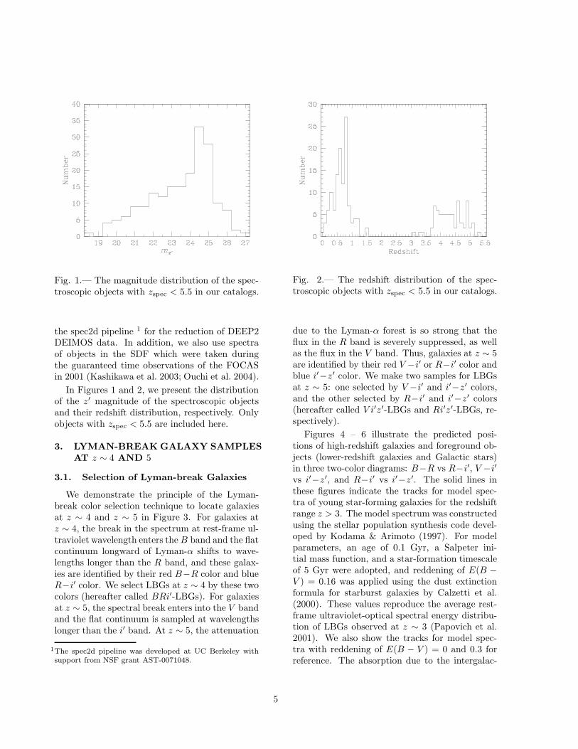
Fig. 1.— The magnitude distribution of the spec-troscopic objects with zspec < 5.5 in our catalogs.

the spec2d pipeline 1 for the reduction of DEEP2DEIMOS data. In addition, we also use spectraof objects in the SDF which were taken duringthe guaranteed time observations of the FOCASin 2001 (Kashikawa et al. 2003; Ouchi et al. 2004).

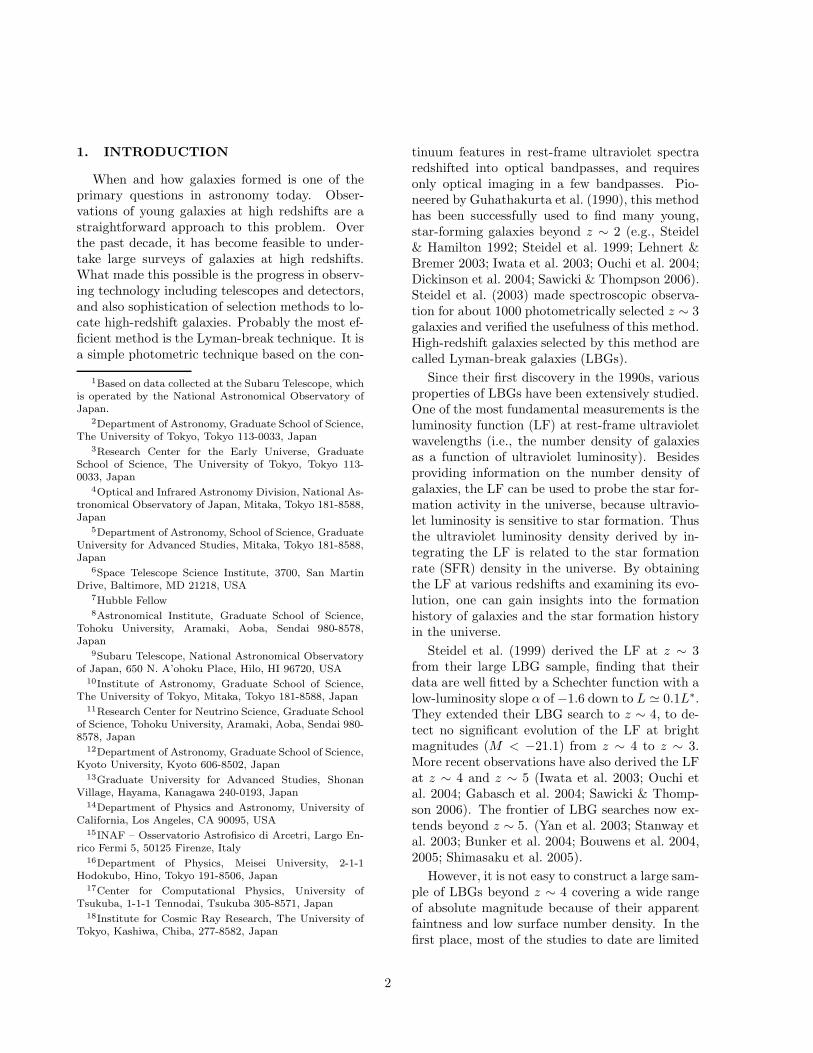
In Figures 1 and 2, we present the distributionof the z′ magnitude of the spectroscopic objectsand their redshift distribution, respectively. Onlyobjects with zspec < 5.5 are included here.

3. LYMAN-BREAKGALAXY SAMPLES

AT z ∼ 4 AND 5

3.1. Selection of Lyman-break Galaxies

We demonstrate the principle of the Lyman-break color selection technique to locate galaxiesat z ∼ 4 and z ∼ 5 in Figure 3. For galaxies atz ∼ 4, the break in the spectrum at rest-frame ul-traviolet wavelength enters the B band and the flatcontinuum longward of Lyman-α shifts to wave-lengths longer than the R band, and these galax-ies are identified by their red B−R color and blueR−i′ color. We select LBGs at z ∼ 4 by these twocolors (hereafter called BRi′-LBGs). For galaxiesat z ∼ 5, the spectral break enters into the V bandand the flat continuum is sampled at wavelengthslonger than the i′ band. At z ∼ 5, the attenuation

1The spec2d pipeline was developed at UC Berkeley withsupport from NSF grant AST-0071048.

Fig. 2.— The redshift distribution of the spec-troscopic objects with zspec < 5.5 in our catalogs.

due to the Lyman-α forest is so strong that theflux in the R band is severely suppressed, as wellas the flux in the V band. Thus, galaxies at z ∼ 5are identified by their red V −i′ or R−i′ color andblue i′−z′ color. We make two samples for LBGsat z ∼ 5: one selected by V −i′ and i′−z′ colors,and the other selected by R−i′ and i′−z′ colors(hereafter called V i′z′-LBGs and Ri′z′-LBGs, re-spectively).

Figures 4 – 6 illustrate the predicted posi-tions of high-redshift galaxies and foreground ob-jects (lower-redshift galaxies and Galactic stars)in three two-color diagrams: B−R vs R−i′, V −i′

vs i′−z′, and R−i′ vs i′−z′. The solid lines inthese figures indicate the tracks for model spec-tra of young star-forming galaxies for the redshiftrange z > 3. The model spectrum was constructedusing the stellar population synthesis code devel-oped by Kodama & Arimoto (1997). For modelparameters, an age of 0.1 Gyr, a Salpeter ini-tial mass function, and a star-formation timescaleof 5 Gyr were adopted, and reddening of E(B −

V ) = 0.16 was applied using the dust extinctionformula for starburst galaxies by Calzetti et al.(2000). These values reproduce the average rest-frame ultraviolet-optical spectral energy distribu-tion of LBGs observed at z ∼ 3 (Papovich et al.2001). We also show the tracks for model spec-tra with reddening of E(B − V ) = 0 and 0.3 forreference. The absorption due to the intergalac-

5

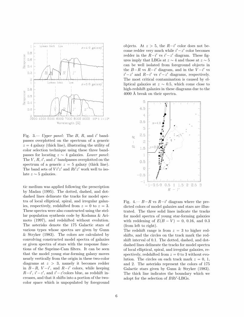
Fig. 3.— Upper panel : The B, R, and i′ band-passes overplotted on the spectrum of a genericz = 4 galaxy (thick line), illustrating the utility ofcolor selection technique using these three band-passes for locating z ∼ 4 galaxies. Lower panel :The V , R, i′, and z′ bandpasses overplotted on thespectrum of a generic z = 5 galaxy (thick line).The band sets of V i′z′ and Ri′z′ work well to iso-late z ∼ 5 galaxies.

tic medium was applied following the prescriptionby Madau (1995). The dotted, dashed, and dot-dashed lines delineate the tracks for model spec-tra of local elliptical, spiral, and irregular galax-ies, respectively, redshifted from z = 0 to z = 3.These spectra were also constructed using the stel-lar population synthesis code by Kodama & Ari-moto (1997), and redshifted without evolution.The asterisks denote the 175 Galactic stars ofvarious types whose spectra are given by Gunn& Stryker (1983). The colors are calculated byconvolving constructed model spectra of galaxiesor given spectra of stars with the response func-tions of the Suprime-Cam filters. It can be seenthat the model young star-forming galaxy movesnearly vertically from the origin in these two-colordiagrams at z > 3, namely it becomes redderin B−R, V −i′, and R−i′ colors, while keepingR−i′, i′−z′, and i′−z′colors blue, as redshift in-creases, and that it shifts into a portion of the two-color space which is unpopulated by foreground

objects. At z > 5, the R−i′ color does not be-come redder very much while i′−z′ color becomesredder in the R−i′ vs i′−z′ diagram. These fig-ures imply that LBGs at z ∼ 4 and those at z ∼ 5can be well isolated from foreground objects inthe B−R vs R−i′ diagram, and in the V −i′ vsi′−z′ and R−i′ vs i′−z′ diagrams, respectively.The most critical contamination is caused by el-liptical galaxies at z ∼ 0.5, which come close tohigh-redshift galaxies in these diagrams due to the4000 A break on their spectra.

Fig. 4.— B−R vs R−i′ diagram where the pre-dicted colors of model galaxies and stars are illus-trated. The three solid lines indicate the tracksfor model spectra of young star-forming galaxieswith reddening of E(B − V ) = 0, 0.16, and 0.3(from left to right).The redshift range is from z = 3 to higher red-shifts, and the circles on the track mark the red-shift interval of 0.1. The dotted, dashed, and dot-dashed lines delineate the tracks for model spectraof local elliptical, spiral, and irregular galaxies, re-spectively, redshifted from z = 0 to 3 without evo-lution. The circles on each track mark z = 0, 1,and 2. The asterisks represent the colors of 175Galactic stars given by Gunn & Stryker (1983).The thick line indicates the boundary which weadopt for the selection of BRi′-LBGs.

6

Fig. 5.— V −i′ vs i′−z′ diagram where the pre-dicted colors of model galaxies and stars are il-lustrated. Lines and symbols are the same as inFigure 4. The thick line indicates the boundarywhich we adopt for the selection of V i′z′-LBGs.

In Figures 7 – 9, we show the distribution ofall the objects contained in the catalogs in thetwo-color diagrams. When the magnitude of anobject in a non-detection band is fainter than the1σ magnitude of the band, the 1σ magnitude is as-signed to the object. Objects with spectroscopicredshifts are shown with colored symbols in thesefigures, where different colors mean different red-shift bins. It is found that the colors of spectro-scopically identified objects match fairly well withthose of model galaxies with corresponding red-shifts in Figures 4 – 6.

We adopt the same color criteria forBRi′-LBGsand V i′z′-LBGs as those of Ouchi et al. (2004).For Ri′z′-LBGs, we visually fine-tune their colorcriteria based on the increased redshift informa-tion. Specifically, we set the selection criteria forBRi′-LBGs as:

B −R > 1.2,

R − i′ < 0.7, (1)

B −R > 1.6(R− i′) + 1.9,

Fig. 6.— R−i′ vs i′−z′ diagram where the pre-dicted colors of model galaxies and stars are il-lustrated. Lines and symbols are the same as inFigure 4. The thick line indicates the boundarywhich we adopt for the selection of Ri′z′-LBGs.

for V i′z′-LBGs as:

V − i′ > 1.2,

i′ − z′ < 0.7, (2a)

V − i′ > 1.8(i′ − z′) + 1.7,

B > 3σ mag, (2b)

and for Ri′z′-LBGs as:

R− i′ > 1.0,

i′ − z′ < 0.7, (3a)

R− i′ > 1.2(i′ − z′) + 0.9,

B, V > 3σ mag. (3b)

The boundaries on the two-color diagrams definedby these color criteria are outlined with the thickorange lines in Figures 4 – 6 and 7 – 9. For thebands which are placed entirely shortward of theLyman break, we additionally require that LBGsshould be non-detected ((2b) and (3b)), which is

7

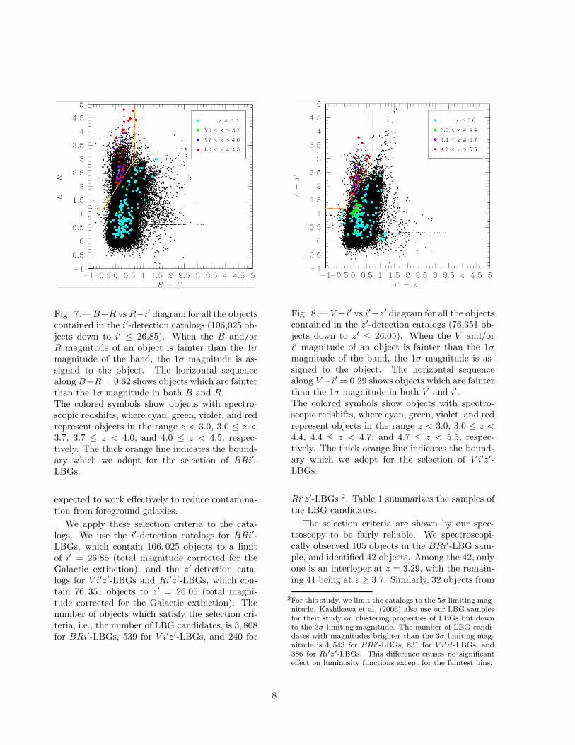
Fig. 7.—B−R vs R−i′ diagram for all the objectscontained in the i′-detection catalogs (106,025 ob-jects down to i′ ≤ 26.85). When the B and/orR magnitude of an object is fainter than the 1σmagnitude of the band, the 1σ magnitude is as-signed to the object. The horizontal sequencealong B−R = 0.62 shows objects which are fainterthan the 1σ magnitude in both B and R.The colored symbols show objects with spectro-scopic redshifts, where cyan, green, violet, and redrepresent objects in the range z < 3.0, 3.0 ≤ z <3.7, 3.7 ≤ z < 4.0, and 4.0 ≤ z < 4.5, respec-tively. The thick orange line indicates the bound-ary which we adopt for the selection of BRi′-LBGs.

expected to work effectively to reduce contamina-tion from foreground galaxies.

We apply these selection criteria to the cata-logs. We use the i′-detection catalogs for BRi′-LBGs, which contain 106, 025 objects to a limitof i′ = 26.85 (total magnitude corrected for theGalactic extinction), and the z′-detection cata-logs for V i′z′-LBGs and Ri′z′-LBGs, which con-tain 76, 351 objects to z′ = 26.05 (total magni-tude corrected for the Galactic extinction). Thenumber of objects which satisfy the selection cri-teria, i.e., the number of LBG candidates, is 3, 808for BRi′-LBGs, 539 for V i′z′-LBGs, and 240 for

Fig. 8.— V −i′ vs i′−z′ diagram for all the objectscontained in the z′-detection catalogs (76,351 ob-jects down to z′ ≤ 26.05). When the V and/ori′ magnitude of an object is fainter than the 1σmagnitude of the band, the 1σ magnitude is as-signed to the object. The horizontal sequencealong V −i′ = 0.29 shows objects which are fainterthan the 1σ magnitude in both V and i′.The colored symbols show objects with spectro-scopic redshifts, where cyan, green, violet, and redrepresent objects in the range z < 3.0, 3.0 ≤ z <4.4, 4.4 ≤ z < 4.7, and 4.7 ≤ z < 5.5, respec-tively. The thick orange line indicates the bound-ary which we adopt for the selection of V i′z′-LBGs.

Ri′z′-LBGs 2. Table 1 summarizes the samples ofthe LBG candidates.

The selection criteria are shown by our spec-troscopy to be fairly reliable. We spectroscopi-cally observed 105 objects in the BRi′-LBG sam-ple, and identified 42 objects. Among the 42, onlyone is an interloper at z = 3.29, with the remain-ing 41 being at z ≥ 3.7. Similarly, 32 objects from

2For this study, we limit the catalogs to the 5σ limiting mag-nitude. Kashikawa et al. (2006) also use our LBG samplesfor their study on clustering properties of LBGs but downto the 3σ limiting magnitude. The number of LBG candi-dates with magnitudes brighter than the 3σ limiting mag-nitude is 4, 543 for BRi′-LBGs, 831 for V i′z′-LBGs, and386 for Ri′z′-LBGs. This difference causes no significanteffect on luminosity functions except for the faintest bins.

8

Fig. 9.— R−i′ vs i′−z′ diagram for all the objectscontained in the z′-detection catalogs (76,351 ob-jects down to z′ ≤ 26.05). When the R and/ori′ magnitude of an object is fainter than the 1σmagnitude of the band, the 1σ magnitude is as-signed to the object. The horizontal sequencealong R−i′ = 0.35 shows objects which are fainterthan the 1σ magnitude in both R and i′.The colored symbols show objects with spectro-scopic redshifts, where cyan, green, violet, and redrepresent objects in the range z < 3.0, 3.0 ≤ z <4.7, 4.7 ≤ z < 4.9, and 4.9 ≤ z < 5.5, respec-tively. The thick orange line indicates the bound-ary which we adopt for the selection of Ri′z′-LBGs.

the V i′z′-LBG sample were spectroscopically ob-served, and 23 were identified. All but one of the23 objects are at z ≥ 4.4; the remaining one ap-pears to be a Galactic star. In the Ri′z′-LBG sam-ple, 12 objects were spectroscopically observed,and 9 were identified. All are found to be atz ≥ 4.5. Possible reasons for the low detectionrate for BRi′-LBGs are that the Lyα emission ofz ∼ 4 LBGs is on average weaker than that ofz ∼ 5 LBGs and that the Lyα line at z ∼ 4 falls inthe wavelength range where the sensitivity of ourspectroscopy is relatively low. The failed samplemay also include interlopers between z ∼ 2 and 3whose strong line features do not enter the wave-length coverage of our spectrograph. From the fol-

lowing simulation, however, we infer that the frac-tion of such interlopers is not so high in our LBGsample. First, we add noise to the colors of all ob-jects outside of the BRi′ selection criteria in ourphotometric catalog according to their measuredmagnitudes. We then count the objects whichnow meet the selection criteria due to the mod-ified colors, to find that they are less than 10% ofthe original LBG candidates even for the faintestmagnitude bin where photometric errors are thelargest. Note that this simulation gives an upperlimit to the fraction of interlopers, since the mea-sured colors already include photometric errors.In Figure 10, we present the apparent magnitudedistribution of the spectroscopically identified ob-jects in each LBG sample. Although the targetsof spectroscopy is biased toward bright objects,we emphasize here that the spectroscopic samplesalso include faint objects and there are no interlop-ers even among them. We cannot, however, ruleout the possibility that there may be interlopersfor which no redshift have been secured. Figure 11shows the redshift distribution of the spectroscopicsamples. The average redshift is < z >spec= 4.1for BRi′-LBGs, < z >spec= 4.8 for V i′z′-LBGs,and < z >spec= 4.9 for Ri′z′-LBGs. Examples ofspectra of z ∼ 4 LBGs and z ∼ 5 LBGs are shownin Figures 12 and 13, respectively.

9

Table 1

Samples of LBG candidates

Sample Name Number of Candidates Detection Band Magnitude Range∗

BRi′-LBG 3,808 i′ i′ = 22.85− 26.85V i′z′-LBG 539 z′ z′ = 23.55− 26.05Ri′z′-LBG 240 z′ z′ = 24.05− 26.05

∗ Total magnitudes corrected for the Galactic extinction.

Fig. 10.— The magnitude distribution of the spec-troscopically identified objects in each LBG sam-ple. Dotted histograms show the magnitude dis-tribution of all the objects in each LBG samplenormalized to the number of the spectroscopicallyidentified objects.

Fig. 11.— The redshift distribution of the spectro-scopically identified objects in each LBG sample.Dotted lines show the redshift distribution func-tions from the Monte Carlo simulation (see §3.3)normalized to the number of the spectroscopicallyidentified objects.

10

Fig. 12.— Examples of spectra of Lyman-breakgalaxies at z ∼ 4 with good quality that haveprominent spectral features such as a strong Lyαemission line and interstellar lines.The lowest panel shows a relative night-sky spec-trum.

3.2. Number Counts

The observed number counts of the LBG can-didates as a function of apparent magnitude areshown in Figures 14 – 16, along with those mea-sured by other authors who selected similar LBGs.None of the data is corrected for contamination orincompleteness. Previous LBG surveys includedin the figures are summarized in Table 2. Ouchiet al. (2004) used the same photometric systems tomake samples of LBGs at z ∼ 4 over a 543 arcmin2

Fig. 13.— Same as Figure 12, but for z ∼ 5.

area and LBGs at z ∼ 5 over a 616 arcmin2 area ofthe SDF. Steidel et al. (1999) carried out a searchfor LBGs at z ∼ 4 using G−R, R−I colors ina total of 828 arcmin2 area of 10 separate fields.Sawicki & Thompson (2006) undertake a survey ofLBGs at z ∼ 4 with the same photometric systemsand selection criteria that Steidel et al. (1999) usebut to a deeper magniude in the Keck Deep Fieldswhich cover a total area of 169 arcmin2 and consistof five fields. Iwata et al. (2003) found LBGs atz ∼ 5 using V −Ic, Ic−z′ colors in a 575 arcmin2

area including the Hubble Deep Field North. Ca-pak et al. (2004) obtained number counts of LBGsat z ∼ 4 selected by B−R, R−Ic colors and LBGsat z ∼ 5 selected by V −Ic, Ic−z′ colors from a 720arcmin2 area centered on the Hubble Deep FieldNorth. Our limiting magnitudes are among thefaintest ones in the LBG samples for z ∼ 4 and 5constructed to date.

In general, number counts measurements ofLBGs are dependent on detection completeness,photometric systems used, and selection crite-ria. It is found that our counts match very wellwith those of Ouchi et al. (2004) for all the sam-ples except for brightest bins. While we useMAG AUTO in SExtractor as total magnitudes ofobjects, Ouchi et al. (2004) calculate total magni-tudes from aperture magnitudes through a fixed

11

Table 2

LBG surveys in the literature

Sample Area [arcmin2] mlimit N Selection Fig. in this paper Ref.

z ∼ 4 875 i′ = 26.85 3, 808 B−R, R−i′ Fig. 14, 19, 21 This studyz ∼ 5 875 z′ = 26.05 539 V −i′, i′−z′ Fig. 15, 20, 21 This studyz ∼ 5 875 z′ = 26.05 240 R−i′, i′−z′ Fig. 16, 20, 21 This study

z ∼ 3 1046 R = 25.5 1, 270 Un−G, G−R Fig. 21 Steidel et al. (1999)z ∼ 4 828 I = 25.0 207 G−R, R−I Fig. 14, 19 Steidel et al. (1999)z ∼ 4 543 i′ = 26.3 1, 438 B−R, R−i′ Fig. 14, 19 Ouchi et al. (2004)z ∼ 4 720 Ic = 25.5 ? B−R, R−Ic Fig. 14 Capak et al. (2004)z ∼ 4 169 R = 27.0 427 G−R, R−I Fig. 19 Sawicki & Thompson (2006)z ∼ 5 575 Ic = 25.95 305 V −Ic, Ic−z′ Fig. 15, 20 Iwata et al. (2003)z ∼ 5 616 z′ = 25.8 246 V −i′, i′−z′ Fig. 15, 20 Ouchi et al. (2004)z ∼ 5 720 Ic = 25.5 ? V −Ic, Ic−z′ Fig. 15 Capak et al. (2004)z ∼ 5 616 z′ = 25.8 68 R−i′, i′−z′ Fig. 16, 20 Ouchi et al. (2004)z ∼ 6 12† z′ = 29.5 506 i−z, V −z Fig. 21 Bouwens et al. (2005)z ∼ 6 767 zR = 25.4 12 i′−zR, zB−zR Fig. 21 Shimasaku et al. (2005)

† Bouwens et al. (2005) incorporated the faint data from the Hubble Ultra Deep Field (12 arcmin2) with two other data sets ofshallower depths: the two GOODS fields (∼ 170 arcmin2 each) and the two Ultra Deep Field-Parallel fields (20 arcmin2 in total).

12

Fig. 14.— Observed number counts of LBGs atz ∼ 4 uncorrected for incompleteness or contami-nation. The filled circles represent the BRi′-LBGsin this study. Comparison is made with the previ-ous measurements obtained by Ouchi et al. (2004)(open circles), Steidel et al. (1999) (open squares),Sawicki & Thompson (2006) (open pentagons),and Capak et al. (2004) (crosses). The error barsfor this study, Ouchi et al. (2004), and Capak etal. (2004) reflect Poisson errors. The error barsfor Steidel et al. (1999) and Sawicki & Thompson(2006) include an estimate of cosmic variance fromtheir multiple fields as well as Poisson errors.

aperture correction of −0.2 mag. The correctionvalue, however, actually can range to as muchas −0.4 mag for bright LBGs. A shift of themagnitudes of Ouchi et al. (2004) by −0.2 mag(= −0.4− (−0.2)) can settle the disagreement be-tween Ouchi et al.’s (2004) and our counts. Thecounts of Capak et al. (2004) are lower than ourcounts for z ∼ 4 widely at faint magnitudes andfor z ∼ 5 at the faintest magnitude of Capak et al.(2004). The lower detection completeness of theirdata might be a major cause of this inconsistency;the 5σ limiting magnitude of their data is about 1mag brighter than that of the SDF Project data.For z ∼ 4 LBGs, our measurements agree withthose of Steidel et al. (1999), although Steidel etal.’s (1999) measurements are limited to objectsbrighter than 25 mag. At faint magnitudes, how-ever, our measurements are higher than those ofSawicki & Thompson (2006). For z ∼ 5 LBGs,over a wide range of bright magnitudes (m < 25),a discrepancy is found between the counts of Iwata

Fig. 15.— Observed number counts of V -dropoutLBGs at z ∼ 5 uncorrected for incompletenessor contamination. The filled circles representthe V i′z′-LBGs in this study. Comparison ismade with the previous measurements obtainedby Ouchi et al. (2004) (open circles), Iwata et al.(2003) (open triangles), and Capak et al. (2004)(crosses). The error bars reflect Poisson errors.

et al. (2003) and either ours or those of Capak etal. (2004) who surveyed almost the same field asIwata et al. (2003); Iwata et al.’s (2003) countsare higher about a factor of 3 – 10. The selec-tion criteria of Iwata et al. (2003) are somewhatlooser than ours. Therefore, as Ouchi et al. (2004)and Capak et al. (2004) claim, the LBG sample ofIwata et al. (2003) could be strongly contaminatedby foreground galaxies.

3.3. Completeness

The completeness at a given apparent magni-tude and redshift is defined as the ratio of LBGswhich are detected and also pass the selection cri-teria, to all the LBGs with the given apparentmagnitude and redshift actually present in theuniverse. In general, completeness decreases asapparent magnitude goes fainter and as redshiftgoes away from the central redshift of the sam-ple. The completeness of each LBG sample is es-timated as functions of apparent magnitude andredshift through a Monte Carlo simulation.

In the simulation, we generate artificial LBGsover an apparent magnitude range of 23.1 ≤ mi′ ≤

26.6 for BRi′-LBGs and 23.8 ≤ mz′ ≤ 25.8 for

13

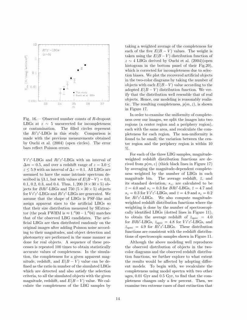
Fig. 16.— Observed number counts of R-dropoutLBGs at z ∼ 5 uncorrected for incompletenessor contamination. The filled circles representthe Ri′z′-LBGs in this study. Comparison ismade with the previous measurements obtainedby Ouchi et al. (2004) (open circles). The errorbars reflect Poisson errors.

V i′z′-LBGs and Ri′z′-LBGs with an interval of∆m = 0.5, and over a redshift range of z = 3.0 ≤

z ≤ 5.9 with an interval of ∆z = 0.1. All LBGs areassumed to have the same intrinsic spectrum de-scribed in §3.1, but with values of E(B−V ) = 0.0,0.1, 0.2, 0.3, and 0.4. Thus, 1, 200 (8× 30× 5) ob-jects for BRi′-LBGs and 750 (5 × 30× 5) objectsfor V i′z′-LBGs and Ri′z′-LBGs are generated. Weassume that the shape of LBGs is PSF-like andassign apparent sizes to the artificial LBGs sothat their size distribution measured by SExtrac-tor (the peak FWHM is ≈ 1.′′00− 1.′′04) matchesthat of the observed LBG candidates. The arti-ficial LBGs are then distributed randomly on theoriginal images after adding Poisson noise accord-ing to their magnitudes, and object detection andphotometry are performed in the same manner asdone for real objects. A sequence of these pro-cesses is repeated 100 times to obtain statisticallyaccurate values of completeness. In the simula-tion, the completeness for a given apparent mag-nitude, redshift, and E(B − V ) value can be de-fined as the ratio in number of the simulated LBGswhich are detected and also satisfy the selectioncriteria, to all the simulated objects with the givenmagnitude, redshift, and E(B−V ) value. We cal-culate the completeness of the LBG samples by

taking a weighted average of the completeness foreach of the five E(B − V ) values. The weight istaken using the E(B−V ) distribution function ofz ∼ 4 LBGs derived by Ouchi et al. (2004)(openhistogram in the bottom panel of their Fig.20),which is corrected for incompleteness due to selec-tion biases. We plot the recovered artificial objectsin the two-color diagrams by taking the number ofobjects with each E(B−V ) value according to theadopted E(B − V ) distribution function. We ver-ify that the distribution well resemble that of realobjects. Hence, our modeling is reasonably realis-tic. The resulting completeness, p(m, z), is shownin Figure 17.

In order to examine the uniformity of complete-ness over our images, we split the images into tworegions (a center region and a periphery region),each with the same area, and recalculate the com-pleteness for each region. The non-uniformity isfound to be small; the variation between the cen-ter region and the periphery region is within 10%.

For each of the three LBG samples, magnitude-weighted redshift distribution functions are de-rived from p(m, z) (thick black lines in Figure 17)by averaging the magnitude-dependent complete-ness weighted by the number of LBGs in eachmagnitude bin. The average redshift, z, andits standard deviation, sz, are calculated to bez = 4.0 and sz = 0.3 for BRi′-LBGs, z = 4.7 andsz = 0.3 for V i′z′-LBGs, and z = 4.9 and sz = 0.2for Ri′z′-LBGs. We also compute magnitude-weighted redshift distribution functions where theweighting is done by the number of spectroscopi-cally identified LBGs (dotted lines in Figure 11),to obtain the average redshift of zspec = 4.0for BRi′-LBGs, zspec = 4.8 for V i′z′-LBGs, andzspec = 4.9 for Ri′z′-LBGs. These distributionfunctions are consistent with the redshift distribu-tions of spectroscopic samples shown in Figure 11.

Although the above modeling well reproducesthe observed distribution of objects in the two-color diagrams and the observed redshift distribu-tion functions, we further explore to what extentthe results would be affected by adopting differ-ent models. To begin with, we recalculate thecompleteness using model spectra with two otherages, 0.01 Gyr and 0.5 Gyr, to find that the com-pleteness changes only a few percent. Then, weexamine two extreme cases of dust extinction that

14

all model spectra have E(B − V ) = 0.0 and 0.4.Changes in completeness are found to be negli-gibly small in either case except for Ri′z′-LBGs.Next, we examine the effect of changing the ab-sorption by the intergalactic medium. If we shiftthe amount of attenuation to ±1σ from the av-erage amount given in Madau (1995), we obtainquite different completeness values. However, theredshift distribution functions derived are unreal-istic, because they are strongly inconsistent withthe distributions of spectroscopic objects. We alsoadopt Meiksin (2006)’s prescription for absorptionby the intergalactic medium, to find completenessvalues similar to those based on Madau (1995)’s.

3.4. Contamination by Interlopers

We estimate the fraction of low-redshift inter-lopers in the LBG samples by a Monte Carlo sim-ulation as follows. For the boundary redshift, z0,between interlopers and LBGs, z0 = 3.5 is adoptedfor BRi′-LBGs, z0 = 4.0 for V i′z′-LBGs, andz0 = 4.5 for Ri′z′-LBGs.

We use objects in the Hubble Deep Field North(HDFN), for which best-fit spectra and photomet-ric redshifts are given by Furusawa et al. (2000),as a template of the color, magnitude, and redshiftdistribution of foreground galaxies, and generate929 artificial objects which mimic the HDFN ob-jects. The apparent sizes of the artificial objectsare adjusted so that the size distribution recov-ered from the simulation is similar to that of thereal objects in our catalogs. We distribute theartificial objects randomly on the original imagesafter adding Poisson noise according to their mag-nitudes, and perform object detection and pho-tometry in the same manner as employed for realobjects. A sequence of these processes is repeated100 times. In the simulation, the number of inter-lopers can be defined as the number of the sim-ulated objects with low redshift (z < z0) whichare detected and also satisfy the selection criteriafor LBGs. The number of interlopers expected inan LBG sample can then be calculated by multi-plying the raw number by a scaling factor whichcorresponds to the ratio of the area of the SDF(875 arcmin2) to the area of the HDFN multipliedby the repeated times (100 × 3.92 arcmin2). Fig-ure 18 shows the fraction of interlopers for ourLBG samples as a function of magnitude. For theBRi′-LBG and Ri′z′-LBG samples, the fraction

is found to be less than 5% at any magnitude.For the V i′z′-LBG sample, the contamination ishigher but at most ≃ 20%. Most of the interlop-ers are in the redshift range of 0.2 ≤ z ≤ 0.8, aspredicted from Figures 4 – 6. The rest are objectsat redshifts which are close to the boundary red-shift of each sample. The fraction of interlopersonly at low redshifts (i.e., not at near the bound-ary redshifts) for each whole sample is around 1%for the BRi′-LBG and Ri′z′-LBG samples, andaround 9% for the V i′z′-LBG sample.

The number density and the redshift distribu-tion of galaxies in the HDFN may be largely differ-ent from the cosmic averages because the HDFNis a very small field. However, the contaminationby interlopers for each of the three LBG samplescalculated above is very low. We therefore ex-pect that the uncertainty in contamination dueto a possible (large) cosmic variance in the HDFNgalaxies will not be a significant source of the er-ror in the luminosity functions of LBGs derived inthe next section.

15

Fig. 17.— Completeness against the redshift ofobjects with different apparent magnitude for ourLBG samples. In the panel of BRi′-LBGs, thered, magenta, green, cyan, blue, red, magenta, andgreen (from top to bottom) lines denote the com-pleteness for i′ = 23.45, 23.95, 24.45, 24.95, 25.45,25.95, 26.45, and 26.95, respectively. In the panelsof V i′z′-LBGs and Ri′z′-LBGs, the red, magenta,green, cyan, and blue lines denote the complete-ness for z′ = 24.15, 24.65, 25.15, 25.65, and 26.15,respectively. The thick black lines in all panelsindicate the magnitude-weighted completeness.

Fig. 18.— Fraction of interlopers as a function ofmagnitude for our LBG samples.

16

4. LUMINOSITY FUNCTIONS AT REST-

FRAMEULTRAVIOLET WAVELENGTHS

We derive the luminosity functions (LFs) ofLBGs at z ∼ 4 – 5 by applying the “effective vol-ume” method (Steidel et al. 1999). The MonteCarlo simulation in §3.3 yields the effective surveyvolume as a function of apparent magnitude,

Veff(m) =

∫ ∞

z0

p(m, z)dV (z)

dzdz, (4)

where p(m, z) is the probability that a galaxy ofapparent magnitude m at redshift z is detectedand passes the selection criteria (i.e., the com-pleteness in §3.3 for magnitude m and redshift z),dV (z)dz is the differential comoving volume at red-

shift z for a solid angle of the surveyed area (875arcmin2), and z0 is the boundary redshift betweenlow-redshift galaxies and LBGs. The effective vol-ume obtained for each magnitude bin is providedin Tables 3 – 5.

The number density of LBGs corrected for in-completeness and contamination is computed as:

φ(m) =Nraw(m)−Ninterloper(m)

Veff(m), (5)

where Nraw(m) and Ninterloper(m) are the numberof LBGs detected and the number of interloperswhich is estimated from the simulations, respec-tively, in an apparent magnitude bin of m. Tables3 – 5 also give Nraw(m) and Ninterloper(m).

The number densities of LBGs in faint bins, es-pecially the faintest bins, could be largely over-estimated owing to Eddington bias from objectsin fainter bins and/or beyond the limiting magni-tude of the sample which have very large photo-metric errors and probably have a larger numberdensity. We evaluate the effect of this bias foreach LBG sample as follows. First, we constructa deeper sample of LBGs down to a magnitudelimit fainter by 0.5 mag than the original value(for example, the new limit is i′ ≤ 27.35 for BRi′-LBGs). Then, using this deeper sample, we carryout Monte Carlo simulations similar to those madein §3.3, and derive Veff(m) to calculate φ(m) to adeeper magnitude. From the simulations, we com-pute for each magnitude bin the fractions of LBGswhich scatter out to other magnitude bins. Fi-nally, we recalculate φ(m) by correcting the origi-nal number densities for the scatter along the mag-

nitude axis. The number density of LBGs derivedin this way is found to be consistent with the orig-inal calculation within statistical errors, down tothe original limiting magnitude. This means thatEddington bias is negligibly small for our samples.

The LF in the rest-frame ultraviolet (≃ 1500 A)absolute magnitude, MUV, is obtained by convert-ing φ(m) into φ(MUV(m)). For each LBG sample,we calculate the absolute magnitude of LBGs fromtheir apparent magnitude using the average red-shift of the sample by

MUV = m+ 2.5 log(1 + z)− 5 log (dL(z)) + 5

+ (mUV −m), (6)

where dL is the luminosity distance in units ofpc. For apparent magnitude, m, we use i′ magni-tude for BRi′-LBGs, and z′ magnitude for V i′z′-LBGs and Ri′z′-LBGs. The last term of Eq.6,(mUV −m), is the difference between the magni-tude at rest-frame 1500A and the magnitude in thebandpass being considered in the rest-frame. Us-ing the representative galaxy models given in §3.1,we find (mUV − m) to be negligible, or no largerthan 0.03 mag, over the redshift ranges selected bythe color selection criteria we adopt. Thus we set(mUV −m) to zero in Eq. 6. We assume that allof the LBGs have the average redshift of the sam-ple. Indeed, for each of the three LBG samples,varying the redshift of an object over the standarddeviation of the redshift distribution of the samplechanges its absolute magnitude by not more than0.1 mag.

In Figures 19 and 20, the LFs at z ∼ 4 andz ∼ 5 are plotted respectively, along with thoseof other authors (See Table 2.). Note that Ca-pak et al. (2004) do not derive the LFs. Our LFsare in excellent agreement with those of Ouchiet al. (2004) up to their faintest magnitudes forboth redshifts. This agreement appears reason-able, since Ouchi et al. (2004) and this study arebased on the same field (the SDF) and adopt al-most the same selection criteria. Our LFs reachfainter magnitudes than theirs. However, thereis a discrepancy between our z ∼ 4 LF and thatof Sawicki & Thompson (2006) in the Keck DeepFields at the faint end; the faint-end slope of ourLF is steeper than that of Sawicki & Thompson(2006). Gabasch et al. (2004) also derived thegalaxy LFs at rest-frame ultraviolet wavelengthsin the FORS Deep Field using photometric red-

17

Table 3

Number of LBGs detected, number of interlopers, and effective survey volume for

BRi′-LBGs.

Magnitude Range (i′) Nrawa Ninterloper

b Veffc

22.85 – 23.35 . . . . . . . . . . . . . . . . . . . . . . 3 0 1.74× 106

23.35 – 23.85 . . . . . . . . . . . . . . . . . . . . . . 12 0 1.63× 106

23.85 – 24.35 . . . . . . . . . . . . . . . . . . . . . . 68 0 1.49× 106

24.35 – 24.85 . . . . . . . . . . . . . . . . . . . . . . 231 0 1.39× 106

24.85 – 25.35 . . . . . . . . . . . . . . . . . . . . . . 447 0 1.22× 106

25.35 – 25.85 . . . . . . . . . . . . . . . . . . . . . . 763 8.9 1.15× 106

25.85 – 26.35 . . . . . . . . . . . . . . . . . . . . . . 1093 24.6 8.77× 105

26.35 – 26.85 . . . . . . . . . . . . . . . . . . . . . . 1191 26.8 5.70× 105

a Number of LBGs detected.

b Number of interlopers estimated from our simulations (see §3.4).

c Effective survey volume for 875 arcmin2 in units of Mpc3.

Table 4


V i′z′-LBGs.

Magnitude Range (z′) Nrawa Ninterloper

b Veffc

23.55 – 24.05 . . . . . . . . . . . . . . . . . . . . . . 1 0 1.34× 106

24.05 – 24.55 . . . . . . . . . . . . . . . . . . . . . . 12 0 1.31× 106

24.55 – 25.05 . . . . . . . . . . . . . . . . . . . . . . 56 0 1.31× 106

25.05 – 25.55 . . . . . . . . . . . . . . . . . . . . . . 152 29.0 1.17× 106

25.55 – 26.05 . . . . . . . . . . . . . . . . . . . . . . 318 22.3 9.66× 105




18

Table 5


Ri′z′-LBGs.

Magnitude Range (z′) Nrawa Ninterloper

b Veffc

24.05 – 24.55 . . . . . . . . . . . . . . . . . . . . . . 3 0 3.32× 105

24.55 – 25.05 . . . . . . . . . . . . . . . . . . . . . . 18 0 4.60× 105

25.05 – 25.55 . . . . . . . . . . . . . . . . . . . . . . 66 2.2 5.54× 105

25.55 – 26.05 . . . . . . . . . . . . . . . . . . . . . . 153 2.2 5.69× 105




shifts and obtained a similar result to that of Saw-icki & Thompson (2006). The reason for this in-consistency is not clear. We note, however, thatour raw counts before the correction of incomplete-ness already exceed the Sawicki & Thompson’s(2006) corrected counts, and thus that our highervalues are not due to overcorrections. Addition-ally, our data have a sky coverage five times largerthan that of the total of the five Keck Deep Fields.Thus, our LF is more robust against a possible cos-mic variance on large scales, although the five sep-arate Keck Deep Fields are less affected by cosmicvariance than a single continuous field of the samesky coverage. At z ∼ 5, our LF is different fromthat of Iwata et al. (2003) at bright magnitudes.One possible explanation for this difference is thatIwata et al. (2003) may select a large number ofcontaminants as mentioned in §3.2, resulting inthe higher number density of bright LBGs.

We find a good agreement between our z ∼ 5LFs obtained from the V i′z′-LBG sample and theRi′z′-LBG sample. The redshift ranges of thesetwo samples are almost the same. This consistencyin the results from the two independent man-ners provides strong support for LFs we obtained.As the V i′z′-LBG sample contains a statisticallylarger number of objects and has higher complete-ness, we only use results from the V i′z′-LBG sam-ple in the following analysis for z ∼ 5. These LFsobtained at z ∼ 4 and 5 are found to be well re-produced by a semi-analytic model combined withhigh-resolution N-body simulations (Nagashima et

al. 2005) when the observational selection effectsare taken into account. We should, however, pointout that the Lyman-break technique cannot se-lect all star-forming galaxies at targeted redshifts.On the basis of spectroscopy of galaxies in anoptically-selected, flux-limited sample, Le Fevre etal. (2005) claim that a large fraction of galax-ies at z ∼ 3 – 4 lie outside the selection bound-aries for LBGs in two-color diagrams. In addition,submm-selected galaxies (e.g., Smail, Ivison, &Blain 1997) and NIR-selected star-forming galax-ies (e.g., Franx et al. 2003) are often too faint inoptical wavelengths to be selected as LBGs, be-cause of strong absorption by dust. Such dustystar-forming galaxies could contribute to the cos-mic SFR density as much as do LBGs (e.g., Chap-man et al. 2005). Therefore, the far UV luminos-ity function and the star formation rate densityderived in this paper are for galaxies with modestdust extinction and passing selection criteria forLBGs, and thus they may be greatly modified ifall star-forming galaxies are included.

We fit the LFs with the Schechter function(Schechter 1976):

φ(L)dL

= φ∗

(

L

L∗

)α

exp

(

−L

L∗

)

d

(

L

L∗

)

, (7)

or expressed in terms of absolute magnitude:

φ(MUV)dMUV

=

(

ln 10

2.5φ∗

)

(

10−0.4(MUV−M∗

UV))α+1

19

Fig. 19.— UV luminosity functions (LFs) of LBGsat z ∼ 4. Our data are shown by the filled circles.The open circles, open squares, and crosses arefrom Ouchi et al. (2004), Steidel et al. (1999), andSawicki & Thompson (2006), respectively. Theerror bars for our data and Ouchi et al.’s (2004)reflect Poisson errors, and those for the other twodata include both Poisson errors and an estimateof field-to-field variance from their multiple fields.

× exp(

−10−0.4(MUV−M∗

UV))

dMUV, (8)

where φ∗, L∗ (M∗UV), and α are parameters to be

determined from the data. The parameter φ∗ isa normalization factor which has a dimension ofnumber density, L∗ is a “characteristic luminos-ity” (with an equivalent “characteristic absolutemagnitude”, M∗

UV), and α gives the slope of theluminosity function at the faint end. For the z ∼ 5LF, whose α has a rather large uncertainty, weevaluate φ∗ and M∗

UV with α fixed to the best-fit value for the z ∼ 4 LF, besides fitting with allthree parameters left free. The best-fit parametersobtained are listed in Table 6.

5. EVOLUTION OF THE COSMIC STAR

FORMATION ACTIVITY OVER 0 ≤

z ≤ 6

5.1. Evolution of the Luminosity Function

We plot the LFs at z ∼ 4 and 5 obtained inthis study with those of LBGs at z ∼ 3 (Sawicki& Thompson 2006) and z ∼ 6 (Bouwens et al.

Fig. 20.— UV luminosity functions (LFs) of LBGsat z ∼ 5. Our data from V i′z′-LBG sample andRi′z′-LBG sample are shown by the filled circlesand filled triangles, respectively. The open circlesand open triangles are from Ouchi et al.’s (2004)V i′z′-LBG sample and Ri′z′-LBG sample, respec-tively. The crosses are from Iwata et al. (2003).The error bars reflect Poisson errors.

2004a; Shimasaku et al. 2005 from observationof the SDF in new filters sensitive to ≃ 1 µm)in Figure 21. The LFs of UV (1500A)-selectedgalaxies at z ∼ 0 (Wyder et al. 2005) and z ∼

1 (Arnouts et al. 2005) are presented as well forreference. Figure 21 reveals clear evolution of theLF beyond z ∼ 4. From z ∼ 4 to z ∼ 3, we findno significant evolution over the whole luminosityrange. Sawicki & Thompson (2006) and Gabaschet al. (2004) detect an increase in faint galaxiesacross this redshift interval, but such an increase isnot seen in our data. At lower redshifts, luminousgalaxies strongly decrease in number from z & 2to z ∼ 0, as has been found by previous studies.

It is unlikely that the evolution in LF seen inFigure 21 is caused by the differences in selectioncriteria among the different samples. We find, us-ing spectra of model galaxies, that the criteria forLBGs at z ∼ 3, 4, and 5 select galaxies over simi-lar ranges of age and E(B − V ). Since i′-dropoutgalaxies at z ∼ 6 are selected with i′ − z′ coloralone, they can have a wide range of E(B − V ).However, since no observation has reported a sig-nificant increase in dust extinction at z > 5, itis reasonable to assume that the i′-dropout galax-

20

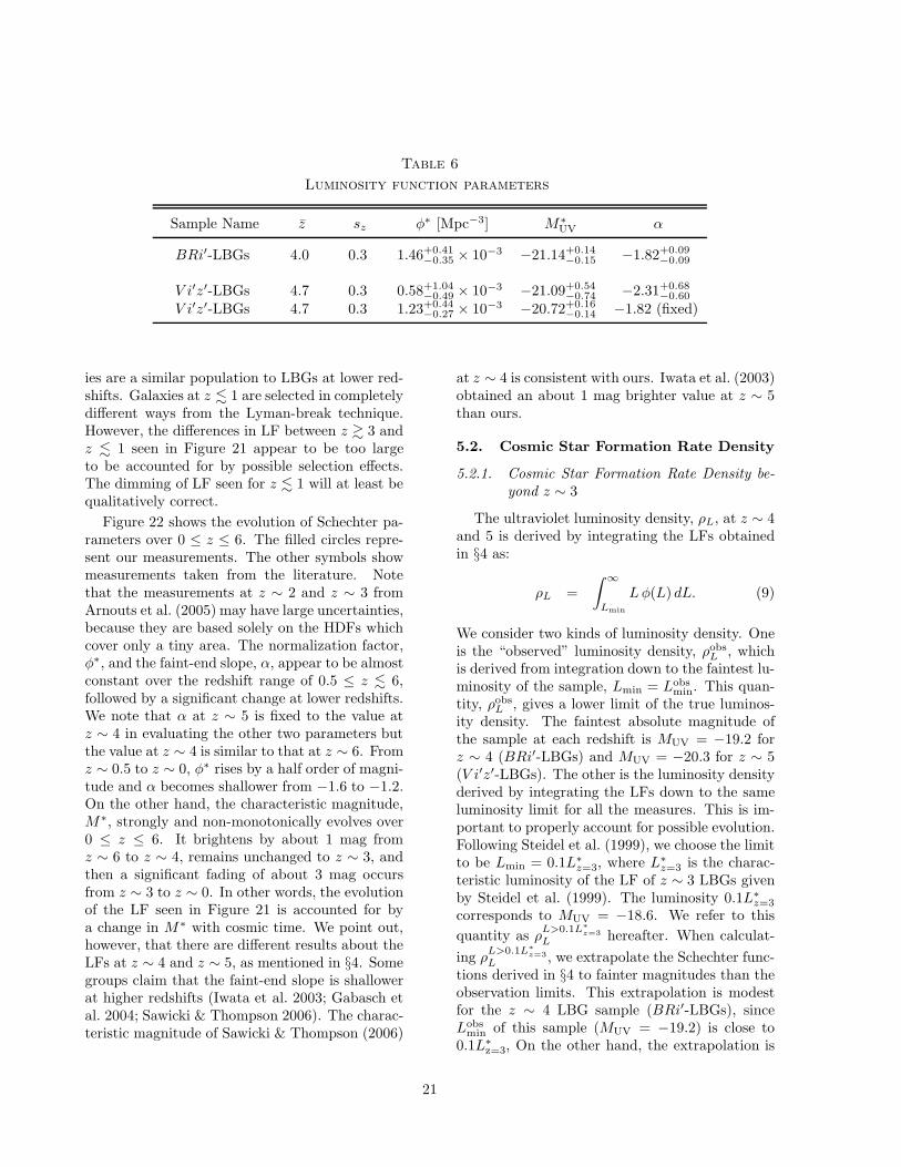
Table 6

Luminosity function parameters

Sample Name z sz φ∗ [Mpc−3] M∗UV α

BRi′-LBGs 4.0 0.3 1.46+0.41−0.35 × 10−3 −21.14+0.14

−0.15 −1.82+0.09−0.09

V i′z′-LBGs 4.7 0.3 0.58+1.04−0.49 × 10−3 −21.09+0.54

−0.74 −2.31+0.68−0.60

V i′z′-LBGs 4.7 0.3 1.23+0.44−0.27 × 10−3 −20.72+0.16

−0.14 −1.82 (fixed)

ies are a similar population to LBGs at lower red-shifts. Galaxies at z . 1 are selected in completelydifferent ways from the Lyman-break technique.However, the differences in LF between z & 3 andz . 1 seen in Figure 21 appear to be too largeto be accounted for by possible selection effects.The dimming of LF seen for z . 1 will at least bequalitatively correct.

Figure 22 shows the evolution of Schechter pa-rameters over 0 ≤ z ≤ 6. The filled circles repre-sent our measurements. The other symbols showmeasurements taken from the literature. Notethat the measurements at z ∼ 2 and z ∼ 3 fromArnouts et al. (2005) may have large uncertainties,because they are based solely on the HDFs whichcover only a tiny area. The normalization factor,φ∗, and the faint-end slope, α, appear to be almostconstant over the redshift range of 0.5 ≤ z . 6,followed by a significant change at lower redshifts.We note that α at z ∼ 5 is fixed to the value atz ∼ 4 in evaluating the other two parameters butthe value at z ∼ 4 is similar to that at z ∼ 6. Fromz ∼ 0.5 to z ∼ 0, φ∗ rises by a half order of magni-tude and α becomes shallower from −1.6 to −1.2.On the other hand, the characteristic magnitude,M∗, strongly and non-monotonically evolves over0 ≤ z ≤ 6. It brightens by about 1 mag fromz ∼ 6 to z ∼ 4, remains unchanged to z ∼ 3, andthen a significant fading of about 3 mag occursfrom z ∼ 3 to z ∼ 0. In other words, the evolutionof the LF seen in Figure 21 is accounted for bya change in M∗ with cosmic time. We point out,however, that there are different results about theLFs at z ∼ 4 and z ∼ 5, as mentioned in §4. Somegroups claim that the faint-end slope is shallowerat higher redshifts (Iwata et al. 2003; Gabasch etal. 2004; Sawicki & Thompson 2006). The charac-teristic magnitude of Sawicki & Thompson (2006)

at z ∼ 4 is consistent with ours. Iwata et al. (2003)obtained an about 1 mag brighter value at z ∼ 5than ours.

5.2. Cosmic Star Formation Rate Density

5.2.1. Cosmic Star Formation Rate Density be-

yond z ∼ 3

The ultraviolet luminosity density, ρL, at z ∼ 4and 5 is derived by integrating the LFs obtainedin §4 as:

ρL =

∫ ∞

Lmin

Lφ(L) dL. (9)

We consider two kinds of luminosity density. Oneis the “observed” luminosity density, ρobsL , whichis derived from integration down to the faintest lu-minosity of the sample, Lmin = Lobs

min. This quan-tity, ρobsL , gives a lower limit of the true luminos-ity density. The faintest absolute magnitude ofthe sample at each redshift is MUV = −19.2 forz ∼ 4 (BRi′-LBGs) and MUV = −20.3 for z ∼ 5(V i′z′-LBGs). The other is the luminosity densityderived by integrating the LFs down to the sameluminosity limit for all the measures. This is im-portant to properly account for possible evolution.Following Steidel et al. (1999), we choose the limitto be Lmin = 0.1L∗

z=3, where L∗z=3 is the charac-

teristic luminosity of the LF of z ∼ 3 LBGs givenby Steidel et al. (1999). The luminosity 0.1L∗

z=3

corresponds to MUV = −18.6. We refer to this

quantity as ρL>0.1L∗

z=3

L hereafter. When calculat-

ing ρL>0.1L∗

z=3

L , we extrapolate the Schechter func-tions derived in §4 to fainter magnitudes than theobservation limits. This extrapolation is modestfor the z ∼ 4 LBG sample (BRi′-LBGs), sinceLobsmin of this sample (MUV = −19.2) is close to

0.1L∗z=3, On the other hand, the extrapolation is

21

Fig. 21.— UV luminosity functions (LFs) of LBGsat z ∼ 3 (blue open circles: Sawicki & Thompson2006),z ∼ 4 (green filled circles: this study [BRi′-LBGs]), z ∼ 5 (red filled circles: this study [V i′z′-LBGs]), and z ∼ 6 (cyan crosses: Bouwens et al.2005; cyan filled triangle: Shimasaku et al. 2005).The error bars reflect Poisson errors. The best-fitSchechter function is also shown with the solid linefor each data set except for that of Shimasaku etal. (2005). The black dashed line and the blackdotted line indicate the LFs of UV-selected galax-ies at z ∼ 0 (Wyder et al. 2005), and z ∼ 1(Arnouts et al. 2005), respectively.

large for the z ∼ 5 LBG sample (V i′z′-LBGs);MUV = −18.6 is fainter than the limiting magni-tude of this sample by 1.7 mag. Table 7 presents

ρobsL and ρL>0.1L∗

z=3

L .

The ultraviolet luminosity density can be usedto measure the star formation rate (SFR) densityin the universe. We compute the cosmic SFR den-sity using the relationship between SFR and ultra-violet luminosity, LUV, given by Kennicutt (1998):

SFR [M⊙ yr−1]

= 1.4× 10−28LUV [ergs s−1 Hz−1]. (10)

This formula assumes a Salpeter initial mass func-tion with 0.1 M⊙ < M < 100 M⊙. The SFRdensity is corrected for dust extinction follow-ing Hopkins (2004), who used the dust extinc-tion formula by Calzetti et al. (2000) and assumedE(B − V ) = 0.128 at all redshifts.

In Figure 23, we show the cosmic SFR densities

Fig. 22.— Evolution of the luminosity functionparameters with time. The filled circles repre-sent the measurements from this study. The othersymbols show measurements taken from the lit-erature: open squares from Wyder et al. (2005),filled squares from Arnouts et al. (2005; GALEX),filled triangles from Arnouts et al. (2005; HDF),open circles from Sawicki & Thompson (2006), andcrosses from Bouwens et al. (2005). For z ∼ 5, wefixed α to the value at z ∼ 4 (α = −1.82) in eval-uating the other two parameters.

obtained in this study as a function of redshift(filled circles), comparing with those calculatedfrom LFs of LBGs at 3 ≤ z ≤ 6 in the literature(other kinds of symbols). We similarly integratetheir LFs down to their observed limiting lumi-nosities to obtain ρobsL and down to L = 0.1L∗

z=3

to obtain ρL>0.1L∗

z=3

L , convert them to the SFRdensities using Eq.(10), and correct for the sameamount of dust extinction to provide a fair com-

parison. The black symbols indicate ρL>0.1L∗

z=3

L ,while the cyan symbols are for the lower limit,ρobsL . Note that the limiting luminosity of the LFat z ∼ 6 by Bouwens et al. (2005) is fainter than

0.1L∗z=3, resulting in ρobsL > ρ

L>0.1L∗

z=3

L . It can

be seen that ρL>0.1L∗

z=3

L is almost constant over3 . z . 5, and perhaps turns to decrease at acertain point between z ∼ 5 and 6. It should

22

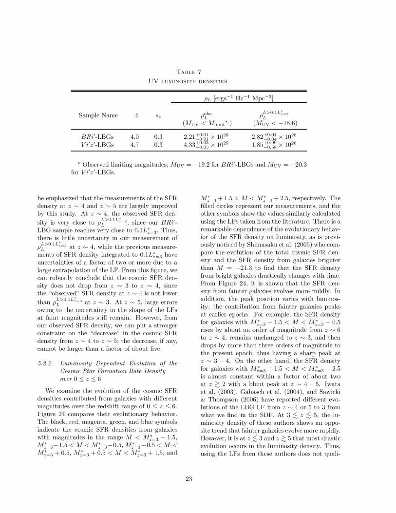
Table 7

UV luminosity densities

ρL [ergs−1 Hz−1 Mpc−3]

Sample Name z sz ρobsL ρL>0.1L∗

z=3

L

(MUV < Mlimit∗ ) (MUV < −18.6)

BRi′-LBGs 4.0 0.3 2.21+0.01−0.01 × 1026 2.82+0.04

−0.04 × 1026

V i′z′-LBGs 4.7 0.3 4.33+0.03−0.05 × 1025 1.85+0.99

−0.58 × 1026

∗ Observed limiting magnitudes; MUV = −19.2 for BRi′-LBGs and MUV = −20.3for V i′z′-LBGs.

be emphasized that the measurements of the SFRdensity at z ∼ 4 and z ∼ 5 are largely improvedby this study. At z ∼ 4, the observed SFR den-

sity is very close to ρL>0.1L∗

z=3

L , since our BRi′-LBG sample reaches very close to 0.1L∗

z=3. Thus,there is little uncertainty in our measurement of

ρL>0.1L∗

z=3

L at z ∼ 4, while the previous measure-ments of SFR density integrated to 0.1L∗

z=3 haveuncertainties of a factor of two or more due to alarge extrapolation of the LF. From this figure, wecan robustly conclude that the cosmic SFR den-sity does not drop from z ∼ 3 to z ∼ 4, sincethe “observed” SFR density at z ∼ 4 is not lower

than ρL>0.1L∗

z=3

L at z ∼ 3. At z ∼ 5, large errorsowing to the uncertainty in the shape of the LFsat faint magnitudes still remain. However, fromour observed SFR density, we can put a strongerconstraint on the “decrease” in the cosmic SFRdensity from z ∼ 4 to z ∼ 5; the decrease, if any,cannot be larger than a factor of about five.

5.2.2. Luminosity Dependent Evolution of the

Cosmic Star Formation Rate Density

over 0 ≤ z ≤ 6

We examine the evolution of the cosmic SFRdensities contributed from galaxies with differentmagnitudes over the redshift range of 0 ≤ z ≤ 6.Figure 24 compares their evolutionary behavior.The black, red, magenta, green, and blue symbolsindicate the cosmic SFR densities from galaxieswith magnitudes in the range M < M∗

z=3 − 1.5,M∗

z=3−1.5 < M < M∗z=3−0.5, M∗

z=3−0.5 < M <M∗

z=3 + 0.5, M∗z=3 + 0.5 < M < M∗

z=3 + 1.5, and

M∗z=3 + 1.5 < M < M∗

z=3 + 2.5, respectively. Thefilled circles represent our measurements, and theother symbols show the values similarly calculatedusing the LFs taken from the literature. There is aremarkable dependence of the evolutionary behav-ior of the SFR density on luminosity, as is previ-ously noticed by Shimasaku et al. (2005) who com-pare the evolution of the total cosmic SFR den-sity and the SFR density from galaxies brighterthan M = −21.3 to find that the SFR densityfrom bright galaxies drastically changes with time.From Figure 24, it is shown that the SFR den-sity from fainter galaxies evolves more mildly. Inaddition, the peak position varies with luminos-ity; the contribution from fainter galaxies peaksat earlier epochs. For example, the SFR densityfor galaxies with M∗

z=3 − 1.5 < M < M∗z=3 − 0.5

rises by about an order of magnitude from z ∼ 6to z ∼ 4, remains unchanged to z ∼ 3, and thendrops by more than three orders of magnitude tothe present epoch, thus having a sharp peak atz ∼ 3 – 4. On the other hand, the SFR densityfor galaxies with M∗

z=3 + 1.5 < M < M∗z=3 + 2.5

is almost constant within a factor of about twoat z & 2 with a blunt peak at z ∼ 4 – 5. Iwataet al. (2003), Gabasch et al. (2004), and Sawicki& Thompson (2006) have reported different evo-lutions of the LBG LF from z ∼ 4 or 5 to 3 fromwhat we find in the SDF. At 3 . z . 5, the lu-minosity density of these authors shows an oppo-site trend that fainter galaxies evolve more rapidly.However, it is at z . 3 and z & 5 that most drasticevolution occurs in the luminosity density. Thus,using the LFs from these authors does not quali-

23

Fig. 23.— Cosmic star formation rate (SFR) den-sity as a function of redshift. The black sym-bols indicate the SFR densities calculated by inte-grating the luminosity functions down to MUV =−18.6 (equivalent to L = 0.1L∗

z=3 from Stei-del et al. 1999), while the cyan symbols showthe lower limits, i.e., the contribution from ac-tually observed galaxies only. The filled circlesrepresent the measurements from this study; theother points come from Steidel et al. (1999) (opensquares), Iwata et al. (2003) (open triangles),Ouchi et al. (2004) (open circles), Gabasch etal. (2004) (open hexagons), Sawicki & Thomp-son (2006) (open pentagons), and Bouwens et al.(2005) (crosses).

tatively change the results on the overall evolutionover 0 . z . 6 obtained here.

This luminosity-dependent evolution of the cos-mic SFR density reflects the evolution of the LFdiscussed in §5.1. The strong increase in the SFRdensity for galaxies brighter than M∗

z=3−0.5 fromz ∼ 6 to z ∼ 3 is due to the brightening ofM∗ withtime. The SFR densities for these bright galaxiesthen drop to the present epoch, as M∗ fades dur-ing the same period. The evolution of the SFRdensities for galaxies fainter than M∗

z=3 − 0.5 ismild, since they are less sensitive to the change inM∗. The earlier peak position of the SFR densityof fainter galaxies suggests that faint galaxies aremore dominant in terms of the cosmic SFR densityat earlier epochs.

We cannot completely rule out the possibilitythat the luminosity-dependent evolution in the

Fig. 24.— Cosmic star formation rate (SFR) den-sity as a function of redshift over the redshiftrange of 0 ≤ z ≤ 6, demonstrating its luminos-ity dependent evolution. The black, red, magenta,green,and blue symbols indicate the SFR densityfrom galaxies with M < M∗

z=3, M∗z=3 − 1.5 <

M < M∗z=3 − 0.5, M∗

z=3 − 0.5 < M < M∗z=3 + 0.5,

M∗z=3+0.5 < M < M∗

z=3+1.5, and M∗z=3+1.5 <

M < M∗z=3 + 2.5, respectively. The filled circles

represent the measurements from this study. Theopen squares comes from Wyder et al. (2005), thefilled squares from Arnouts et al. (2005; GALEX),the filled triangles from Arnouts et al. (2005;HDF), the open circles from Sawicki & Thomp-son (2006),and the crosses from Bouwens et al. (2005).

cosmic SFR density seen above is not real butreflects luminosity-dependent evolution of someother properties such as dust extinction. If, forinstance, galaxies have the smallest dust extinc-tion at z ∼ 3 – 4, then the observed M⋆ will bethe brightest at these redshifts, as seen in Fig-ure 22, even if the intrinsic, dust-corrected M⋆

does not change with redshift. In this case, thebehavior of the luminosity-dependent SFR den-sity will be qualitatively similar to that found inFigure 24. However, no observation has reportedstrong evolution of E(B − V ) at least for LBGs.The E(B − V ) distribution of LBGs appears tobe unchanged over z ∼ 5 and 3 (Iwata et al. 2003;Ouchi et al. 2004). In addition, E(B−V ) is known

24

to be independent of apparent M (Adelberger &Steidel 2000; Ouchi et al. 2004).

5.3. Specific Star Formation Rate

We explore the evolution of what we define asthe specific SFR here, i.e., the cosmic SFR perunit baryon mass in dark haloes. The specificSFR means the efficiency of star formation aver-aged over the all dark haloes present at a givenredshift. The specific SFR is computed by divid-

ing the cosmic SFR density, ρL>0.1L∗

z=3

L , by theaverage mass density of baryons confined in darkhaloes, ρb. Here, ρb is calculated by

ρb(z) =Ωb

Ωm

∫ ∞

Mmin(z)

n(M, z)M dM, (11)

where Ωb = 0.05 is the density parameter ofbaryons, n(M, z) is the mass function of darkhaloes at redshift z predicted by the standard ColdDark Matter model with σ8 = 0.9, Mmin(z) isthe halo mass corresponding to a virial temper-ature of 1× 104 K. We assume here that gas doesnot cool (and thus stars are not formed) in darkhaloes with T < 1 × 104 K. Note that Mmin(z) ismuch smaller than the estimated mass of haloeswhich host the faintest galaxies we account here,i.e., galaxies with 0.1L∗

z=3.

Figure 25 shows the evolution of the specificSFR over 0 ≤ z ≤ 6. The filled circles representour measurements and the other symbols show thevalues from the literature. The dotted line in thefigure shows (1 + z)3 evolution. We find that thespecific SFR increases in proportion to (1 + z)3

up to z ∼ 4. In other words, the star formationefficiency in the universe rises with redshift. Atz & 4, on the other hand, the specific SFR appearsto decrease.

Here, according to the standard Cold DarkMatter model, the average internal density inphysical units of baryons in dark haloes virializedat a given redshift,

⟨

ρDHb

⟩

, is known to be approx-imately proportional to the average mass densityof the universe at that time, and the average massdensity of the universe changes as (1+z)3. There-fore, it implies that the specific SFR increases ap-proximately in proportion to

⟨

ρDHb

⟩

up to z ∼ 4.To put it another way, since the specific SFR isthe internal density of SFR in dark haloes,

⟨

ρDHSFR

⟩

,

divided by⟨

ρDHb

⟩

, this result can be expressed in

Fig. 25.— Specific star formation rate (SFR) ver-sus (1 + z) over 0 ≤ z ≤ 6. Symbols are the sameas in Figure 24. The dotted line shows evolutionin power-law, specific SFR ∝ (1 + z)3.

terms of⟨

ρDHSFR

⟩

and⟨

ρDHb

⟩

as:

⟨

ρDHSFR

⟩

∝⟨

ρDHb

⟩2. (12)

It is surprising that the star formation in galaxiesobeys such a simple power law over 90% of thecosmic history (0 < z . 4). Equation (12) resem-bles the Schmidt law (Schmidt 1959) of nearbydisk galaxies, a relationship between the disk-averaged SFR and cold gas surface densities ofΣSFR = const. × ΣN

gas with N ∼ 1.4 (Kennicutt1998).

We present here one possible explanation of theobserved behavior of the specific SFR. The ana-lytical modeling of galaxy formation based on theCDMmodel by Hernquist & Springel (2003) showsthat the gas cooling rate, Mcool/MDH, of darkhaloes roughly scales with H(z)2, or equivalentlywith (1 + z)3 as H(z) is approximately propor-tional to (1 + z)3/2 in our cosmology. They alsofind that the star formation rate in dark haloesscales with the cooling rate at low and interme-diate redshifts, while it becomes to be no longerdependent on the cooling rate at redshifts largerthan a certain limit, where the internal density ofhaloes is so high that the cooling time is shorterthan the consumption rate of cooled gas into stars.If we adopt this modeling, then our result impliesthat the cosmic SFR is primarily determined bythe gas cooling rate at z . 4, while it is governed

25

by the conversion rate of cooled gas into stars atlarger redshifts.

Of course, the cooling rate may not be the ma-jor factor determining the cosmic star formationrate. There are many other factors on which thestar formation in galaxies can largely depends,such as the feedback by galactic winds, the UVbackground radiation field, and environmental ef-fects like galaxy merging and interactions. Sincethe relative importance of these factors will varywith the mass of dark haloes, it will be interestingto measure the specific SFR as a function of halomass.

6. SUMMARY AND CONCLUSIONS

We investigated the luminosity functions andstar formation rates of Lyman-break galaxies(LBGs) at z ∼ 4 and 5 based on the optical imag-ing data obtained in the Subaru Deep Field (SDF)Project. The SDF Project is a program conductedby Subaru Observatory to carry out a deep andwide galaxy survey in the SDF.

Three samples of LBGs in a contiguous 875arcmin2 area are constructed. One consists ofLBGs at z ∼ 4 selected with the B−R vs R−i′

diagram (BRi′-LBGs). The other two consist ofLBGs at z ∼ 5 selected with two kinds of two-color diagrams: V −i′ vs i′−z′ (V i′z′-LBGs) andR−i′ vs i′−z′ (Ri′z′-LBGs). The number of LBGsdetected is 3, 808 for BRi′-LBGs, 539 for V i′z′-LBGs, and 240 for Ri′z′-LBGs. The adopted se-lection criteria are proved to be fairly reliable bythe spectroscopic data. We use Monte Carlo simu-lations to estimate the completeness and the frac-tion of contamination by interlopers. The redshiftdistribution functions obtained by the simulationsare well consistent with the redshift distributionsof spectroscopically identified objects in the LBGsamples.

We derived the luminosity functions at rest-frame ultraviolet wavelengths down to as faint asMUV = −19.2 at z ∼ 4 and MUV = −20.3 atz ∼ 5. The cosmic star formation rate (SFR) den-sity was measured from the ultraviolet luminositydensity derived by integrating the luminosity func-tions. On the basis of the observed SFR densityand the standard Cold Dark Matter model, thecosmic SFR per unit baryon mass in dark haloes,i.e., the specific SFR, is computed. Combining

the results obtained in this work with those takenfrom the literature, we reached the following con-clusions:

(i) Clear evolution of the luminosity function isdetected. The characteristic magnitude M∗

changes strongly over the redshift range of0 ≤ z ≤ 6. It brightens by about 1 mag fromz ∼ 6 to z ∼ 4, remains unchanged to z ∼ 3and then fades by about 3 mag from z ∼ 3 toz ∼ 0. On the other hand, the normalizationfactor, φ∗, and the faint-end slope, α, arealmost constant over 0.5 . z . 6.

(ii) The measurements of the SFR density atz ∼ 4 and z ∼ 5 are greatly improved, sincethe luminosity functions are derived downto very faint magnitudes. Hence, the evolu-tionary behavior of the SFR density is moreconstrained. The cosmic SFR density doesnot drop from z ∼ 3 to z ∼ 4, and the de-crease from z ∼ 4 to z ∼ 5, if any, cannot belarger than a factor of about five.

(iii) The SFR density contributed from brightergalaxies changes more drastically with cos-mic time. The contribution from galaxiesbrighter than M∗

z=3 − 0.5 has a sharp peakaround z = 3 – 4, while that from galax-ies fainter than M∗

z=3−0.5 evolves relativelymildly with a broad peak at earlier epoch.This luminosity-dependent evolution of thecosmic SFR density suggests that the galaxypopulation that contributes to the total SFRdensity in the universe varies with time, re-flecting the evolution of the luminosity func-tion.

(iv) The specific SFR is found to scale with red-shift as (1 + z)3 up to z ∼ 4, implying thatthe efficiency of star formation is on aver-age higher at higher redshift in proportion tothe cooling rate within dark haloes. It seemsthat this is not simply the case at z & 4.

We would like to thank the referee for valuablecomments and suggestions. We are deeply grate-ful to the Subaru Telescope staff for their devotedsupport in this project.

26

REFERENCES

Adelberger, K. L. & Steidel, C. C. 2000, ApJ, 544,218

Arnouts, S., et al. 2005, ApJ, 619, L43

Bertin, E. & Arnouts, S. 1996, A&AS, 117, 393

Bouwens, R. J., et al. 2004, ApJ, 616, L79

Bouwens, R. J., Illingworth, G. D., Blakeslee, J.P., & Franx, M. 2005, ApJ, in press (astro-ph/0509641)

Bunker, A. J., Stanway, E. R., Ellis, R. S., &McMahon, R. G. 2004, MNRAS, 355, 374

Calzetti, D., Armus, L., Bohlin, R. C., Kinney,A. L., Koornneef, J., & Storchi-Bergmann, T.2000, ApJ, 533, 682

Capak, P., et al. 2004, AJ, 127, 180

Chapman, S. C., Blain, A. W., Smail, I., & Ivison,R. J. 2005, ApJ, 622, 772

Dickinson, M., et al. 2004, ApJ, 600, L99

Faber, S. M., et al. 2003, Proc. SPIE, 4841, 1657

Franx, M., et al. 2003, ApJ, 587, L79

Furusawa, H., Shimasaku, K., Doi, M., & Oka-mura, S. 2000, ApJ, 534, 624

Gabasch, A., et al. 2004, A&A, 421, 41

Guhathakurta, P., Tyson, J. A., & Majewski, S.R. 1990, ApJ, 357, L9

Gunn, J. E. & Stryker, L. L. 1983, ApJS, 52, 121

Hernquist, L. & Springel, V. 2003, MNRAS, 341,1253

Hopkins, A. M. 2004, ApJ, 615, 209

Iwata, I., Ohta, K., Tamura, N., Ando, M., Wada,S., Watanabe, C., Akiyama, M., & Aoki, K.2003, PASJ, 55, 415

Iye, M., et al. 2004, PASJ, 56, 381

Kashikawa, N., et al. 2002, PASJ, 54, 819

Kashikawa, N., et al. 2003, AJ, 125, 53

Kashikawa, N., et al. 2004, PASJ, 56, 1011

Kashikawa, N., et al. 2006, ApJ, in press (astro-ph/0509564)

Kennicutt, R. C., Jr. 1998, ARA&A, 36, 189

Kodama, T. & Arimoto, N. 1997, A&A, 320, 41

Le Fevre, O., et al. 2005, Nature, 437, 519

Lehnert, M. D. & Bremer, M. 2003, ApJ, 593, 630

Madau, P. 1995, ApJ, 441, 18

Maihara, T., et al. 2001, PASJ, 53, 25

Meiksin, A. 2006, MNRAS, 365, 807

Nagashima, M., Yahagi, H., Enoki, M., Yoshii,Y., & Gouda, N. 2005, ApJ, in press (astro-ph/0508085)

Miyazaki, S., et al. 2002, PASJ, 54, 833

Oke, J. B. & Gunn, J. E. 1983, ApJ, 266, 713

Ouchi, M. 2003, Ph.D. Thesis, The University ofTokyo

Ouchi, M., et al. 2004, ApJ, 611, 660

Papovich, C., Dickinson, M., & Ferguson, H. C.2001, ApJ, 559, 620

Sawicki, M. & Thompson, D. 2006, ApJ, 642, 653

Shimasaku, K., Ouchi, M., Furusawa, H., Yoshida,M., Kashikawa, N., & Okamura, S. 2005, PASJ,57, 447

Schechter, P. 1976, ApJ, 203, 297

Schlegel, D. J., Finkbeiner, D. P., & Davis, M.1998, ApJ, 500, 525

Schmidt, M. 1959, ApJ, 129, 243

Smail, I., Ivison, R. J., & Blain, A. W. 1997, ApJ,490, L5

Spergel, D. N., et al. 2003, ApJS, 148, 175

Stanway, E. R., Bunker A. J., & McMahon, R. G.2003, MNRAS, 342, 439

Steidel, C. C. & Hamilton, D. 1992, AJ, 104, 941

Steidel, C. C., Adelberger, K. L., Giavalisco, M.,Dickinson, M., & Pettini, M. 1999, ApJ, 519, 1

27

Steidel, C. C., Adelberger, K. L., Shapley, A. E.,Pettini, M., Dickinson, M., & Giavalisco, M.2003, 592, 728

Wyder, T. K., et al. 2005, ApJ, 619, L15

Yagi, M., Kashikawa, N., Sekiguchi, M., Doi, M.,Yasuda, N., Shimasaku, K., & Okamura, S.2002, AJ, 123, 66

Yan, H., Windhorst, R. A., & Cohen, S. H. 2003,ApJ, 585, L93

This 2-column preprint was prepared with the AAS LATEXmacros v5.2.

28

Luminosity Functions of Lyman-Break Galaxies at z~ 4 and 5 in the ...

Documents

Transcript of Luminosity Functions of Lyman-Break Galaxies at z~ 4 and 5 in the ...