The Luminosity Function of Cluster Galaxies. III. I. Parolin et al.: The Luminosity Function of...

arX

iv:a

stro

-ph/

0306

508v

1 2

4 Ju

n 20

03Astronomy & Astrophysicsmanuscript no. paper June 1, 2018(DOI: will be inserted by hand later)

The Luminosity Function of Cluster Galaxies. III.

I. Parolin1, E. Molinari1, and G. Chincarini1,2

1 INAF - Osservatorio Astronomico di Brera, Via Bianchi 46, 23807 Merate (LC), Italy2 Universita degli Studi di Milano-Bicocca, Piazza dell’Ateneo Nuovo 1, 20126, Milano, Italy

Received March 12, 2003; accepted June 09, 2003

Abstract. We investigated the optical properties of 7 clusters of galaxies observed in three colors over the range of absolutemagnitudes−24 ≤ M ≤ −12. Our aim is to estimate the Luminosity Function and the total cluster luminosity of our samplein order to have information about the formation and the evolution of galaxies in clusters. In this paper, we present the mainpoints of our analysis and give the formal parameters obtained by fitting the data using the maximum likelihood algorithm. Wefind consistency between our results and other works in literature confirming the bimodal nature of the luminosity function ofcluster galaxies. More important, we find that the relation Lopt/LX versus LX is color dependent: Low X ray Luminosity clustershave a bluer galaxy population.

Key words. Galaxies: luminosity function, mass function – Galaxies: clusters, general

1. Introduction

The estimate of the total cluster luminosity in different colors,the estimate of its Luminosity Function (LF) and the compar-ison with the LF of field galaxies (see also Chincarini (1988))are powerful tools to gather information on how a cluster ofgalaxies forms, evolves and accretes from the field.

Currently, we have at least two determinations of the formof the local field LF (Binggeli et al. 1988) which are in excel-lent agreement: Zucca et al. (1997) and Blanton et al. (2001).Blanton et al. (2001) estimate the local field LF in differentcolors down to an absolute magnitude M∼ −16 (Petrosianmagnitudes) using the Sloan Digital Sky Survey (SDSS)commissioning data. The very large sample they used al-lowed them to have very good statistics and they estimated:φ = (1.46± 0.12) · 10−2h3Mpc−3, M∗(r) = −20.83± 0.03,α = −1.20± 0.03. These values are comparable with theones found by Zucca et al. (1997), who analysed the localfield LF down to magnitudes M∼ −12 through the ESOSlice Project (ESP) survey:φ = (0.020± 0.004)h3Mpc−3,M∗(Bj) = −19.61± 0.07, α = −1.22± 0.06. The data fromthe ESP survey, four magnitudes deeper than SDSS, showeda steepening of the faint-end slope starting at magnitudeMBj ∼ −17 that Zucca et al. fitted with a power law withslopeβ = −1.6. In spite of the small number of objects withMBj ≥ −16, this is a very important result, as it is in line withthe value found by Driver et al. (1994), and it is in contrastwith the value that Loveday & al. (1992), obtained from a

Send offprint requests to: I. Parolin, e-mail:[email protected]

shallower survey, and highlights the need for further studies ofthe faint-end slope, at least down to magnitudes M∼ −12.

We believe that we have a fair knowledge of the local fieldLF, even though future surveys will provide better details,es-pecially at faint luminosities. Naturally, the number of lowsurface-brightness galaxies (LSB) we miss and the number ofcompact galaxies that could be confused with stars are stillun-known.According to Caldwell & Bothun (1987), LSB galaxies aredestroyed near the cluster center more likely than normalgalaxies, and form a diffuse stellar background followingthe cluster potential. The compact galaxies, thanks to theirstrong density gradient, will survive also if their number isvery high in a cluster, as found by Chincarini & Rood (1972),Gavazzi et al. (2002) and Sakai et al. (2002). Undoubtedly, theanalysis of the complete SDSS will give an important step for-ward in solving these problems.

For clusters of galaxies the situation is more com-plex. A milestone in the study of the LF is the cata-logue by Binggeli et al. (1985 a,b) and the related analysis bySandage et al. (1985). For the first time, they understood therole that the different types of galaxies play in the LF. Theyfound that the faint end, clearly dominated by dwarf galaxies,had a rather high slope ofα ∼ −1.4.Because of the closeness of the Virgo cluster, these worksshould be taken as a firm reference point, and every study of theLF of cluster galaxies must be aware of the difficulties in de-tecting and measuring LSB galaxies (Impey & Bothun (1997)).

A large amount of work has been published on the LF ofcluster galaxies and we will discuss the recent literature in a

http://arxiv.org/abs/astro-ph/0306508v1

2 I. Parolin et al.: The Luminosity Function of Cluster Galaxies. III.

comparative way in a forthcoming paper. To give a short surveyof the situation, we refer here to a few works.

Studying A 963 (z∼ 0.2), Driver et al. (1994) find a re-sult that coincides very well with the early work on Coma(z ∼ 0.02) by Godwin & Peach (1977), and with the LF func-tion derived for A 2554 (z∼ 0.01, Smith et al. (1997)). Theiranalysis on the sample, that reaches MR = −16.5, shows a LFthat could be fit by a composition of two Schechter functions,or by a Schechter plus a power law, with slope−1 and−1.8respectively (in reasonable agreement with the findings fromthe Virgo cluster and by the ESP in the field). Also, this workoutlines the uncertanties related to the background subtraction(Driver et al. (1994 Fig. 5a); see also Bernstein et al. (1995)).As also shown by Abell et al. (1989), the background densityof galaxies is uncertain by a factor of the order of the effectwe measure and shows changes from region to region. Frompublished studies and from our own work, this seems to be themain source of bias in determining the slope of the LF faintend.

To better distinguish between the probable cluster mem-bers and the background, Biviano et al. (1995), used the red-shift data in their work on Coma. Obviously, this would bethe way to go, but generally redshifts are not available forthe faintest objects. The spectroscopic sample used by Bivianoet al., reaches magnitude Mb = −16.9 (assuming for Comam−M = 34.9 with Ho= 75km/s/Mpc), with a completenessof about 95%. To extend the analysis to fainter magnitudes,M ∼ 15.5, they added 205 galaxies selected by photometric cri-teria and the faint end slope they measure is aboutα ∼ −1.3.

Further confirmation of those results was obtained byBernstein et al. (1995), who used the deepest observationsavailable of the Coma cluster (down to MR = −9.4). Theywere not able to measure a detailed LF on the bright end,but found a slopeα = −1.42± 0.05 in the magnitude range−19.4 < MR < −11.4, and a sharp steepening of the LF be-yond that range. This probably recalls the old problem posedby Zwicky (1972 - private communication) about the faint endof the LF: where does it end and what kind of objects populateit.At faint magnitudes, it’s indeed hard to distinguish the faint-magnitude objects of the cluster from background objects with-out high resolution imaging and spectra.

Another interesting result has been pointed out byBarkhouse et al. (2002). They analyzed a very large sample ofcluster galaxies with the same purpose as ours, that is to de-termine if the faint-end slope is a function of the cluster mor-phology and if there is a gradient in the faint end slope of theLF moving from the central cluster regions toward the out-skirt. They seem to have reached some positive evidence onthose effects even if they do not go very deep in magnitudes(MR < −16). Finally, analysing the LF of the first cluster of oursample, A496, Molinari et al. (1998), found a clear evidenceofbimodal LF and a quite high faint end slope (α = −1.65).

2. The luminosity Function

The detailed description of the observations, the data analy-sis and the algorithms we used can be found in the papers by

Molinari et al. (1998), Moretti et al. (1999), and the laureathe-sis by Moretti (1997), Ratti (1998), and Parolin (2002). As wewant to present the results from the analysis of 7 clusters oftheoriginal sample, we give here just few informations to ease thereading (see Table 1).

We carried out the observations at ESO, La Silla, atthe Danish 1.54 m Telescope using the Danish Faint ObjectSpectrograph and Camera (DFOSC) and theg, r and i col-ors of the Gunn’s photometric system (Thuan & Gunn 1976;Wade et al. 1979).

After a standard reduction of the data, for each clusterwe created a catalogue of sources by merging the photo-metrical catalogue of the bright and extensive galaxies ob-tained through a program specifically developed by Moretti etal.(1999) with the photometrical catalogue of small and faintobjects obtained using the MIDAS Inventory package. Infact,as Inventory was developed to detect sources in distant clus-ters (point-like sources), we first extracted and analysed all thebright and extended galaxies through the program by Morettiet al. (1999), that reproduces the image of a galaxy through theFourier analysis of its isophotes and subtracts it to the mainframe, then applied Inventory.The catalogs thus created were tested through a series of sim-ulations, briefly described below, to evaluate their complete-ness: using one of the galaxies reproduced with the programby Moretti et al. divided by coefficients ad hoc, we created asample of artificial galaxies with a known distribution of mag-nitudes. We partitioned the field to be tested in circular annuliin which we added the artificial sample with known randomcoordinates; by running Inventory on the added fields we wereable to estimate the selection function as a function of the dis-tance of the cluster center.

After that, we carried out our analysis.

2.1. The standard analysis

To sharpen the contrast between the counts in the cluster andthe counts in the field, we selected those galaxies that in thecolor magnitude plot are placed in between the 68% confidencecurves defined by the line fitting ther versus(g-r) distribu-tion of bright galaxies (the equivalent of the E/S0 sequence asdefined by Visvanatan & Sandage (1977)) and its rms (Fig. 1).These galaxies, mostly ellipticals, have indeed a higher proba-bility to be cluster members.

This area is defined by the curves:

C = a ·m+ q± (k · σfit + σ0) (1)

Where the term a·m+ q represents the fit of the color-magnitude relation for galaxies brighter than r= 19 andσ0 =

√(σ2

g + σ2r ) is the color index error derived using the

magnitude error estimated on the fields overlapping in the dif-ferent frames.Non-members may perturb the fit to derive the coefficientsaandq, also in view of the small number of stars which belongsto the bright sequence, so we coupled the regression solutionwith the best fit as estimated by eye.

We assumed that all the galaxies which in the color-magnitude diagram belong to this region form what we will

I. Parolin et al.: The Luminosity Function of Cluster Galaxies. III. 3

Cluster α2000 δ2000 Redshift B.M. type Abell type

Abell 0085 00h41m50.11s -09d18m17.5s 0.05560 I 2Abell 0133 01h02m42.21s -21d52m43.5s 0.05660 I 2EXO 0422-086 04h25m51.02s -08d33m38.5s 0.03971 I-II -Abell 3667 20h12m35.08s -56d50m30.5s 0.05560 II 2Abell 3695 20h34m46.86s -35d49m07.5s 0.08930 I 2Abell 4038 23h47m41.78s -28d08m26.5s 0.02920 I-II 2Abell 4059 23h57m00.02s -34d45m24.5s 0.04600 I 1

Table 1. The 7 clusters analized in this paper.

12 14 16 18 20 22 2410

0

101

102

103

104

105

106

magnitude

coun

ts

r bkgi bkgg magr magi mag

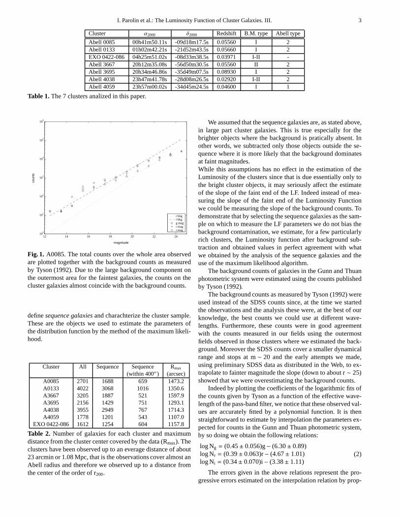
Fig. 1. A0085. The total counts over the whole area observedare plotted together with the background counts as measuredby Tyson (1992). Due to the large background component onthe outermost area for the faintest galaxies, the counts on thecluster galaxies almost coincide with the background counts.

definesequence galaxies and charachterize the cluster sample.These are the objects we used to estimate the parameters ofthe distribution function by the method of the maximum likeli-hood.

Cluster All Sequence Sequence Rmax

(within 400′′) (arcsec)A0085 2701 1688 659 1473.2A0133 4022 3068 1016 1350.6A3667 3205 1887 521 1597.9A3695 2156 1429 751 1293.1A4038 3955 2949 767 1714.3A4059 1778 1201 543 1107.0

EXO 0422-086 1612 1254 604 1157.8

Table 2. Number of galaxies for each cluster and maximumdistance from the cluster center covered by the data (Rmax). Theclusters have been observed up to an everage distance of about23 arcmin or 1.08 Mpc, that is the observations cover almost anAbell radius and therefore we observed up to a distance fromthe center of the order of r200.

We assumed that the sequence galaxies are, as stated above,in large part cluster galaxies. This is true especially for thebrighter objects where the background is pratically absent. Inother words, we subtracted only those objects outside the se-quence where it is more likely that the background dominatesat faint magnitudes.While this assumptions has no effect in the estimation of theLuminosity of the clusters since that is due essentially only tothe bright cluster objects, it may seriously affect the estimateof the slope of the faint end of the LF. Indeed instead of mea-suring the slope of the faint end of the Luminosity Functionwe could be measuring the slope of the background counts. Todemonstrate that by selecting the sequence galaxies as the sam-ple on which to measure the LF parameters we do not bias thebackground contamination, we estimate, for a few particularlyrich clusters, the Luminosity function after background sub-traction and obtained values in perfect agreement with whatwe obtained by the analysis of the sequence galaxies and theuse of the maximum likelihood algorithm.

The background counts of galaxies in the Gunn and Thuanphotometric system were estimated using the counts publishedby Tyson (1992).

The background counts as measured by Tyson (1992) wereused instead of the SDSS counts since, at the time we startedthe observations and the analysis these were, at the best of ourknowledge, the best counts we could use at different wave-lengths. Furthermore, these counts were in good agreementwith the counts measured in our fields using the outermostfields observed in those clusters where we estimated the back-ground. Moreover the SDSS counts cover a smaller dynamicalrange and stops at m∼ 20 and the early attempts we made,using preliminary SDSS data as distributed in the Web, to ex-trapolate to fainter magnitude the slope (down to about r∼ 25)showed that we were overestimating the background counts.

Indeed by plotting the coefficients of the logarithmic fits ofthe counts given by Tyson as a function of the effective wave-length of the pass-band filter, we notice that these observedval-ues are accurately fitted by a polynomial function. It is thenstraightforward to estimate by interpolation the parameters ex-pected for counts in the Gunn and Thuan photometric system,by so doing we obtain the following relations:

log Ng = (0.45± 0.056)g− (6.30± 0.89)log Nr = (0.39± 0.063)r− (4.67± 1.01)log Ni = (0.34± 0.070)i− (3.38± 1.11)

(2)

The errors given in the above relations represent the pro-gressive errors estimated on the interpolation relation byprop-


agating the errors of the fits relating the parameters to the ef-fective wavelength of the filters used by Tyson.

14 15 16 17 18 19 20 21 22 2310

0

101

102

103

104

105

mr

coun

ts/d

egre

e2

r bkgr mag

Fig. 2. A0085. Counts in the r filter limited to the central framecompared to the background counts as given by Tyson (1992).The cluster signal is well visible over the background.

We modeled the distribution in luminosity by using a bi-variate LF that is the sum of a Gaussian and a Schechter.The choice is the most reasonable one following the work bySandage et al. (1985) on the Virgo cluster; it is evident fromthedata of the present analysis, Fig. 1 and Fig.2 and as indicatedalso in Molinari et al. (1998) and references therein. In a clus-ter, as it is very evident also from our data, the bright galaxiesare located in the central region and these are the galaxies thatare fitted by the Gaussian component of the LF. That is the twocomponent fit is valid only for the central region, in the out-skirts of the cluster the luminosity of the galaxies is distributedaccording only to the Schechter function (Fig. 8).

We are aware that not all of the published analysis on the LFof clusters of galaxies, such as the one of Goto et al. (2002),ev-idence the bimodal distribution. While it is hard to answer whywithout remaking the analysis and eventually the data reduc-tion, it seems to us that the main reasons reside on the statistics,accuracy of the magnitudes and background subtraction and,inpart, from the binning. Indeed from a practical point of view,and looking at it in a slightly different way, the main evidencedepends from the small “gaps” in the observed distributionwhich is evidenced in the point where the composite functionsare both somewhat weaker. In our cluster sample this occurs atther mag which is in the range 17−18. Obviously in a redshiftsample the signal vs. noise ratio is large due to a better selec-tion of cluster members detaching the cluster galaxies almostcompletely from the background. Indeed this is clearly shownalso by the Coma sample selected by Biviano et al. (1995) andby the sample in Moretti et al. (1999). On the other hand theanalysis of Goto et al. (2002) based on the SDSS survey clearlyshows that a) the analysis is consistent with the distribution oftwo underlying populations, b) the analysis deals with the com-posite LF so that details are smoothed out adding the contribu-

tion of different clusters and c) the limiting magnitude is notfaint enough (the sample stops at M∼ −18) to clearly definethe faint end.

For the Maximum Likelihood fitting we used only objectsbrighter than the 14th magnitude. This means that we excludedthe cD (in two clusters this cut off excludes 2 or 3 galaxies)from the fitting. The cD does not necessarily conform to a dis-tribution function as the other galaxies and its luminositymaybe a function not only of the cluster mass distribution at thetime of formation but, above all, may reflect the characteris-tics of evolution. While it is easy to account for its luminosity,it is a perturbing factor in the fitting. The cD galaxies will bediscussed in detail in a forthcoming paper.

We analyzed all the clusters in a similar way to have inter-nal consistency. In most cases, two of the authors analyzed theclusters and compared the results to have an estimate of howmuch the result could depend from our method of analysis andhave, at the same time, an estimate for the uncertainties. The re-sults of the standard analysis are listed in Tables 3 and 4. Usingthese values and the master photometric catalogues we derivedthe Luminosities listed in Table 5.

3. Checking our analysis, a few test cases

In this section, we illustrate part of the data and our analysisalso evidencing some weak points. While the standard analy-sis was done in a very homogeneous and systematic way, formost of the clusters we used alternative analysis, that is a)weestimated the luminosity function subtracting from the centralframe the counts as given by Tyson (1992); b) we subtractedthe background using the outermost field we observed wherethe cluster galaxies contamination is known to be negligible.In all these cases, after the subtraction of the background,theLF parameters were estimated after binning the derived his-togram, assumed to represent statistically the counts of thecluster galaxies, and using aχ2 minimizaton program.

As it is explained below, it makes a difference whether ornot the cD galaxy is part of the sample. Furthermore, and asexpected, if the analysis is not limited to the central region, ofthe order of a core radius, the contrast cluster vs. backgroundis largely washed out. But, as described in the following text,the best evidence that the bimodal distribution is a real fact isillustrated in the lower panel of Fig. 5. Here the contaminationof the background galaxies brighter than the 21st magnitudeis negligible and the maximum of the Gaussian distribution isreadily visible at r∼ 16 while it is also clearly visible the brightend of the LF and to the low number of galaxies expected to-ward the faint end of the Gaussian distribution.

Since all the set of clusters used to test the method weretreated in a similar way, for each cluster we discuss only partof it in order to give a complete view of the tests we made inoder to develop a feeling for the robustness of our results. Bydoing so we also avoid useless duplications. We also definitelythink that the standard analysis and the results we give in Tables3 and 4 represent the consistent results, with their errors,thatare the output of this work and that is why we prefer not toconfuse the issue by listing the derivation of the parameters by


other methods that while in agreement within errors with thestandard analysis are less homogeneous and rigorous.

3.1. A0085

In Fig. 1 we plot the total counts, that is the counts made overthe whole observed area of our sample, for the 3 colors used(g, r and i), as a function of the magnitudes. Moreover, weplot the counts for the field as derived using the analysis byTyson (1992), in the filterr andi.Our counts do not differ much from the background from onefilter to the other. The larger discrepancy is with thei filter inwhich we count more than 30% of galaxies less than in theother filters. A probable cause for this is the high sky back-ground and the lower quality of these frames. However, wewant to evidence the excess of counts (bump) compared to thebackground at magnitude∼ 15 that is due to the cluster we ob-served.If we plot only the central field, the contrast cluster/backgroundincerases considerably and it evidences indeed the fact that thecluster galaxy counts can be clearly separated. This is naturallywhat we expect. Assuming a King’s density profile the percent-age of cluster galaxies we would expect on the outermost fieldwe observed in the different clusters is of about 10% so thathere the backgrounds dominates. Indeed, and always to checkout procedures, we also estimated the cluster galaxies countsby subtracting the outermost field from the central once assum-ing that the small cluster contamination on the background sodefined would not bias the estimate od the cluster LF. We gota good agreement, for those clusters which were analysed alsoin this way, with the standard analysis.

The bright end is most highly dominated by cluster galaxiesas we expect a small number of field galaxies in such a limitedvolume of space.

After the correction for completeness, it is straightforwardto estimate the cluster contribution by subtracting the fieldcounts. However, by doing so, we are more sensitive to thefluctuations of the background and to an eventual uncontrolledincompleteness introduced by our analysis. Furthermore, at thebright end we are dealing with a few objects, and the low statis-tics make things more uncertain. That is why we decided to useonly relative measurements and, to further increase the contrastcluster versus field, to use only a selected subsample of galaxiesfor each cluster delimited by the fitting of the bright sequencegalaxies and the 1σ error.

As we explained earlier, we define a color-magnitude se-quence via the color magnitude diagram for each filter and foreach cluster. In the case of ther observations for the clusterA0085, Fig. 1, the lines delimiting the sequence galaxies areaare defined by:

(g− r)seq= −0.0180· r + 0.802σerr−cur = (g− r)seq± (0.117+ 0.675· 0.217)

For this cluster, we used a factor 0.675 to reduce to 50% theprobability that a galaxy belongs to the sequence with the com-puted rms. We also extended the sequence multiplying by a fac-tor 3 the value ofσfit to increase the number of sources at thefaint end and to ease the comparison with the other clusters (in

−1.5 −1 −0.5 0 0.5 1 1.5 2

12

14

16

18

20

22

24

26

g−r

mr

Fig. 3. The color magnitude plot for the central area of the clus-ter A0085. The plot illustrates the fit, shown here as a dashedblack line, that determines the sequence galaxies as describedin the text. The solid lines, as described in the text, define 68%probability that the objects has a color-magnitude as defined bythe sequence.

particular A4059). These minor adjustments do not affect thederivations of the parameter in which we are interested. On theother hand, they are selected during the analysis to optimize thestatistics and the homogeneity of the solution. Two membersof our group derived the luminosity function both using the se-quence we just defined and all of the central field objects. Thischecking analysis was also carried out using theχ2 method andsubtracting the background. For the faint end of the LF, the re-sulting slopes were all very similar to that obtained with thestandard analysis. In all cases, we obtained similar and consis-tent results within the errors, an evidence that the resultsaregood and practically unaffected by the method of the analysis.

3.2. A0133

With this cluster we had some difficulties in getting a reason-able fit of the observed LF in spite of the large number of mea-surements. As we did for most of the clusters, we carried outthe fits in the different wavelengths deriving the parameters ofthe LF:

a) for all the galaxies in the central field after subtractingthebackground;

b) for the sequence galaxies of the cluster after backgroundsubtraction;

c) for the counts derived as the difference between the centralfield and the outermost field (for the clusters for which wecould use the latter as a background).

In spite of the large uncertainties, we derived the same parame-ters within errors with all methods. Finally, the various sampleswere tested for solution in a semi-empirical way. The countsas a function of the magnitudes, were fitted by modifying theparameters derived statistically and estimating the best fit, or


0 0.5 1 1.5 2 2.5 3

0

0.5

1

1.5

2

2.5

g−i

g−r

color−color model (without evolution)galaxies with m

r<19

Fig. 4. Color-color plot of A0085. The bright sequence galaxieslays exactly on the color-color curve generated by the modelsof synthesis. Naturally, the sub-sample sequence fits as wellwith a broader dispersion and reflects the color-color cuts weimposed in the definition of the sequence.

the different fits, also by eye. This procedure, that we describeonly for A0133, was indeed carried out for most of the sampleclusters. The reason is that in some cases the parameters wederived formally using the Maximum Likelihood have large er-rors. This is especially true for the magnitude of the knee oftheSchechter function or for the ratio of the Gauss to the Schechternormalization factor. By doing so we hoped to avoid flukes dueto the analysis and to the small counts and to make sure whichparameters must be taken with caution. What remains certain,however, is that the LF is in all cases dominated by a ratherbroad Gaussian defined by the brightest galaxies and dominat-ing over the Schechter function which is essentially definedbythe fainter galaxies. The cD galaxy does not fit the LuminosityFunction.

3.3. A4038

With a completeness down to the 22nd magnitude in the centralregion and down to the 23rd magnitude in the outskirts (upperpanel of Fig. 5), A4038 is a clear example of the bimodal dis-tribution function.

The lower panel of Fig. 5 shows the color-magnitude plotof the sequence galaxies. We see quite clearly the increase firstand the decrease later of the number density of galaxies alongthe sequence going from brighter to fainter magnitudes, andthis effect has been observed in all clusters and in all the col-ors. At about r= 19, we find the so calledgap, that is the regionin the LF where the Gauss distribution dominating at brightmagnitudes merges with, and is taken over, by the Schechterdistribution.In the outermost field of this cluster the background, as esti-mated by Tyson (1992), is somewhat higher than our counts forr ≥ 21.5. This outlines that at faint magnitudes we are strongly

200

400

600

r

23.25

23.5

23.75

Magnitude

0.99

0.995

1

% Detec.

200

400

600

r

0.99

0.995

−1.5 −1 −0.5 0 0.5 1

12

14

16

18

20

22

24

26

g−r

mr

Fig. 5. Abell 4038. Upper panel: the completeness Function forthe r filter as a function of the distance from the cluster cen-ter (in seconds of arc). Lower panel: the distribution of these-quence galaxies shows that the number density, and thereforethe distribution function we derived, is composed by a con-densation of bright objects and by a multitude of faints objectswhose number increases with the magnitude.

affected by the fluctuations of the background and by incom-pleteness.

3.4. A4059

We use of this cluster to discuss in more detail the fit and relateduncertainties on the study of the LF of clusters. These uncer-tainties are not due to pure statistics, but rather to the selectedprocedures. As usual, we illustrate ther filter observations foruniformity with the previous, and following,discussion. Asim-ilar analysis has been done and checked in all colors on vari-ous clusters obtaining consistent results. That is to say that thegoodness of the parameters values obtained and the proceduresdiscussed is robust.

In Fig. 6, we plot both the data obtained by subtracting thebackground as estimated by Tyson (1992) and that derived byour data using the outermost field observed (as we stated earlierhere we have a cluster galaxies contamination of about 50%).


12 14 16 18 20 2210

0

101

102

103

r mag

coun

ts

Fig. 6. A4059. The black filled diamonds refer to the countsin the central 400” frame after subtracting the counts byTyson (1992), while the empty dots refer to the same countsafter subtraction of the outermost field we observed for thiscluster. The solid line reflects the values derived from a semiempirical fit of the data. The dash line show the Gaussian dis-tribution selected and the fit of the faint end by a straight (dot)line. The fit has been obtained using the following values forthe LF parameters: G/S= 350.0/150.0, mG = 16.3, σG = 1.0,mS = 18.0 andα = −1.5. The cD galaxy does not fit the LF.

The Tyson Background is somewhat higher, the difference be-ing probably due to fluctuations. Contrary to what has beendone for standard solution, in the distribution in Fig. 6 we alsoincluded the cD galaxy that, being too bright, does not fit theLF, no matter which parameters we select.

At the faint end we obtain a fit of the counts that is in ex-cellent agreement with the value obtained using the MaximumLikelihood method applied to the sequence galaxies. This jus-tifies the method once more and underlines that we derive re-liable values also for the faint end in spite of correcting onlypartially for the background galaxies.

However, to stress the subtleness of the faint end fittingin presence of a background contamination, we point out thatthis slope can easily be estimated by a linear fit of the faintgalaxies. The faint end of the Schechter function expressedin magnitude and on a logarithmic scale is given by the re-lation −0.4 · (m−m∗) · (α + 1) so thatα can be derived by asimple linear fit of the faint end of the observed distributionusing the relation:α = − (1+ (observed slope/0.4)). The back-ground can also readily checked and subtracted since we sim-ply make the difference between two straight lines. Assumingthe counts are dominated by background objects, we wouldhaveobserved slope = 0.39 and deriveα > −1.5 and closer to−2.

4. The cluster luminosity: the contributions of thebright and the faint end

An estimate of the luminosity of a cluster is given by simplyintegrating the Cluster LF, in absolute magnitudes, using thefollowing expressions:

LS = −1.086·∫

L2L∗

L1L∗

(

LL∗

)α+1· e

−LL∗ d(

LL∗

)

LG = −2.5 ·∫ log L2

log L1L · ρ · e

−0.5·(

−2.5(log L−log LG)σG

)2

d(log L)(3)

where L1 > L2 and wherermρ is the Gaussian/Schechter nor-malization ratio.

As we said before, in the expression of the LF the faint endis the greater source of uncertainties because of the backgroundfluctuations and of the uncertainties in the estimate of the com-pleteness (the estimate of the selection function remains oftenuncertain in spite of the Monte Carlo approach which is less ro-bust when applied near the core area where many bright galax-ies are located).

−2.2 −2 −1.8 −1.6 −1.4 −1.2 −1 −0.80.3

0.4

0.5

0.6

0.7

0.8

0.9

1

α

Lum

inos

ity R

atio

(G

auss

/Tot

al)

ρ = 2.0ρ = 1.0ρ = 0.7ρ = 0.4ρ = 0.2

Fig. 7. The Ratio between the luminosity contained in brightgalaxies fitted by a Gaussian LF and the total luminosity(Gaussian+ Schechter function) as a function of the param-eterα and the normalization ratio between the Gaussian andthe Schechter function,ρ in the equation. From top to bottomρ = 2.0, 1.0, 0.7, 0.4, 0.2 .

It seems that the cluster luminosity is dominated by thebright galaxies. In Fig. 7 for various values of the ratio be-tween the Gaussian and the Schechter normalization, we plotthe percentage of the total cluster luminosity which is due tothe bright galaxies as fitted by a Gaussian. We used a magni-tude difference< MGauss> −M∗Schechter= 1.5. This difference isclose to what we find in some of our clusters. In the Virgo clus-ter, Sandage et al. (1985), find< MGauss> −M∗Schechter= 0.9.However, the ratio is practically not affected very much by suchdifferences. As it can be seen from Fig. 7, what counts is mainlythe normalization ratio and the value of the faint end slopeα.Disregarding extreme values, that isρ > 1, which have beenhowever also observed in our clusters, we find that forα ∼ −1.4


the ratio varies between 0.6 and 0.85 while for α ∼ −1 theratio changes between 0.74 and 0.92. Clearly, in those caseswhereρ > 1, the Gaussian distribution function contributiondominates. In the Virgo cluster (Sandage et al. 1985) we esti-mateρ ∼ 0.14. However, in this clusterσG is rather large whileα ∼ −1.35 close to what has been found in the majority of theclusters.

Merging clusters, or more precisely clusters for which sub-structures are detected, do not affect the estimate of the totalluminosity and the LF. During the merging of substructures weexpect changes in luminosity of the galaxies due to inducedtides and therefore luminosities for the merging galaxies thatdiffer somewhat for the luminosities of the merged galaxies.On the other hand this effect, which likely result in a loss ofstars to the Intra-Cluster Medium (ICM) and at the same timebrightening and star formation due to the induced turbolence inthe Interstellar Medium (ISM), is a secondary, not detectableeffect to the analysis of this work.

We calculated that an estimate of the cluster luminosity us-ing only the bright galaxies as fitted by a Gaussian plus a stan-dard slope faint end luminosity function gives a mean error ofabout 10%. In all those cases in which there are uncertaintiesin the faint end fitting or we notice the presence of a greaterbackground contamination, we estimated, as a check, also thetotal luminosity by using mean parameters for the faint end ofthe LF.

In general, the procedure we followed is the following:

- We used the cluster parameters as derived from the standardanalysis

- We normalized the luminosity function by subtracting theluminosity derived by the counts of the background as es-timated by Tyson (1992) from the counts we have for eachcluster in a given range of magnitudes selected ad hoc (therange is not critical):g < 19.5, r < 19 andi < 19.

- We limited the normalization to the bright galaxies in orderto avoid further uncertainties due to the background and thesubtraction of large numbers at faint magnitudes.

- In most cases, we based the normalization on the Gaussiancomponent since the ratio of the Gaussian to Schechter wasestimated from the fit, albeit with large error in some cases.For the normalization, we used only the frame about thecluster center.

- For each cluster we also counted and selected the galaxiesin the range of apparent magnitude corresponding toMg <

−16.5, Mr < −17.0 andMi < −17.0 and we simply addedup the relative luminosities.

We observe a clear difference between the central part ofthe cluster, where the bright galaxies dominate, and the out-skirts, where the central part of the cluster bright galaxies aregenerally absent. This is a strong evidence of segregation in lu-minosity and is consistent with the model of a fairly relaxedcluster of galaxies. That has been taken into account in com-puting the cluster luminosity.

To better account for this difference we adopted a model inwhich the number density distribution follows a King’s profileand the LF changes from a Gaussian plus a Schechter (where

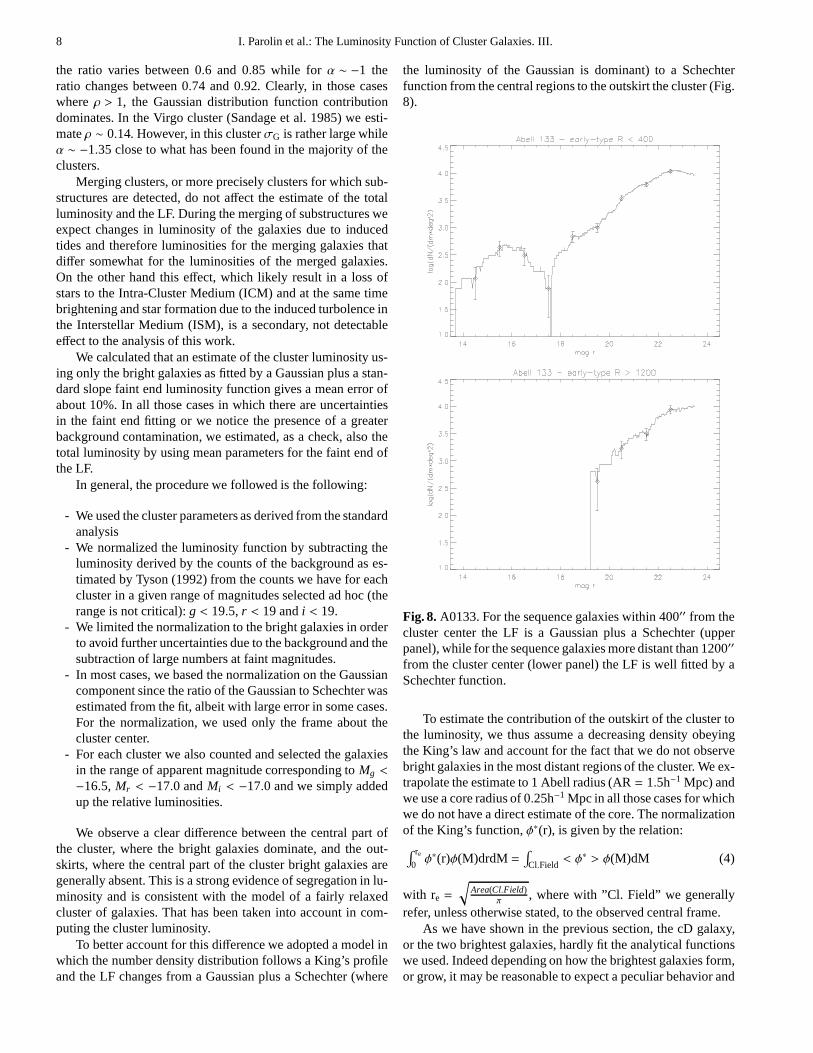
the luminosity of the Gaussian is dominant) to a Schechterfunction from the central regions to the outskirt the cluster (Fig.8).

Fig. 8. A0133. For the sequence galaxies within 400′′ from thecluster center the LF is a Gaussian plus a Schechter (upperpanel), while for the sequence galaxies more distant than 1200′′

from the cluster center (lower panel) the LF is well fitted by aSchechter function.

To estimate the contribution of the outskirt of the cluster tothe luminosity, we thus assume a decreasing density obeyingthe King’s law and account for the fact that we do not observebright galaxies in the most distant regions of the cluster. We ex-trapolate the estimate to 1 Abell radius (AR= 1.5h−1 Mpc) andwe use a core radius of 0.25h−1 Mpc in all those cases for whichwe do not have a direct estimate of the core. The normalizationof the King’s function,φ∗(r), is given by the relation:∫ re

0φ∗(r)φ(M)drdM =

∫

Cl.Field< φ∗ > φ(M)dM (4)

with re =

√

Area(Cl.Field)π

, where with ”Cl. Field” we generallyrefer, unless otherwise stated, to the observed central frame.

As we have shown in the previous section, the cD galaxy,or the two brightest galaxies, hardly fit the analytical functionswe used. Indeed depending on how the brightest galaxies form,or grow, it may be reasonable to expect a peculiar behavior and


disagreement with the analytical function. In other words theanalytical fit may underestimate the Luminosity because sucha bright galaxy is not expected by the distribution. To com-pute the luminosity, the LF has been considered in the rangebetween M= −12 and M= −24.

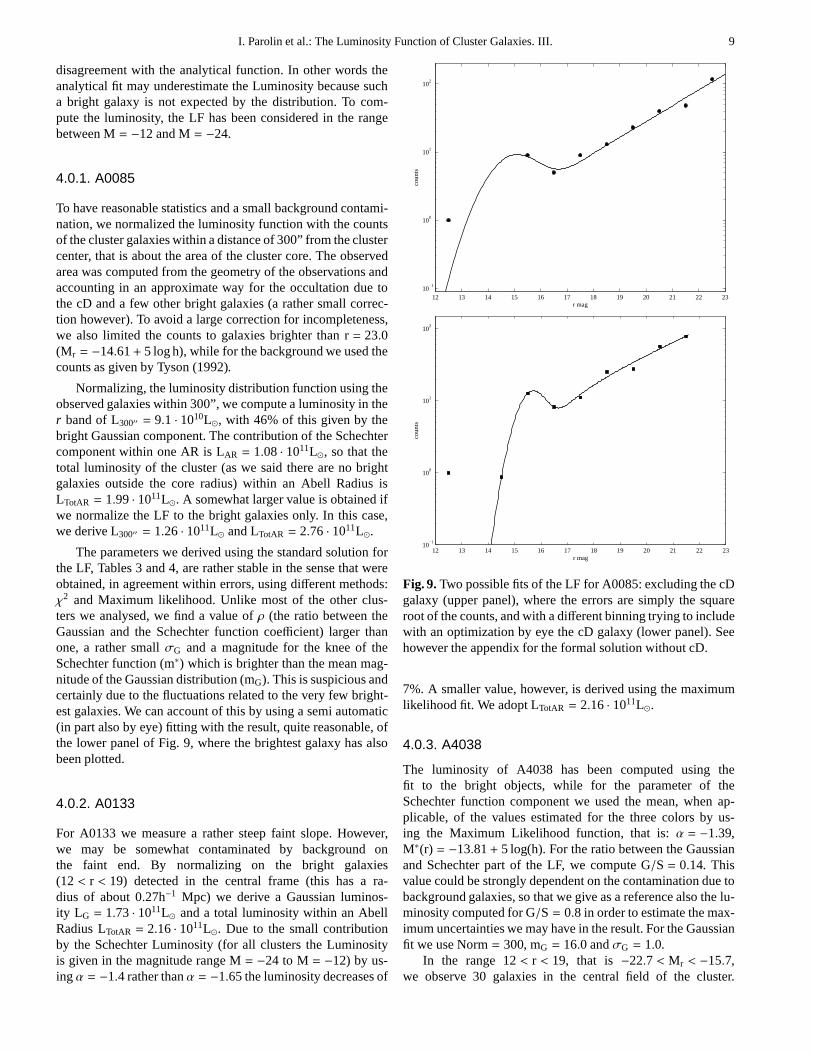
4.0.1. A0085

To have reasonable statistics and a small background contami-nation, we normalized the luminosity function with the countsof the cluster galaxies within a distance of 300” from the clustercenter, that is about the area of the cluster core. The observedarea was computed from the geometry of the observations andaccounting in an approximate way for the occultation due tothe cD and a few other bright galaxies (a rather small correc-tion however). To avoid a large correction for incompleteness,we also limited the counts to galaxies brighter than r= 23.0(Mr = −14.61+ 5 log h), while for the background we used thecounts as given by Tyson (1992).

Normalizing, the luminosity distribution function using theobserved galaxies within 300”, we compute a luminosity in ther band of L300′′ = 9.1 · 1010L⊙, with 46% of this given by thebright Gaussian component. The contribution of the Schechtercomponent within one AR is LAR = 1.08 · 1011L⊙, so that thetotal luminosity of the cluster (as we said there are no brightgalaxies outside the core radius) within an Abell Radius isLTotAR = 1.99 · 1011L⊙. A somewhat larger value is obtained ifwe normalize the LF to the bright galaxies only. In this case,we derive L300′′ = 1.26 · 1011L⊙ and LTotAR = 2.76 · 1011L⊙.

The parameters we derived using the standard solution forthe LF, Tables 3 and 4, are rather stable in the sense that wereobtained, in agreement within errors, using different methods:χ2 and Maximum likelihood. Unlike most of the other clus-ters we analysed, we find a value ofρ (the ratio between theGaussian and the Schechter function coefficient) larger thanone, a rather smallσG and a magnitude for the knee of theSchechter function (m∗) which is brighter than the mean mag-nitude of the Gaussian distribution (mG). This is suspicious andcertainly due to the fluctuations related to the very few bright-est galaxies. We can account of this by using a semi automatic(in part also by eye) fitting with the result, quite reasonable, ofthe lower panel of Fig. 9, where the brightest galaxy has alsobeen plotted.

4.0.2. A0133

For A0133 we measure a rather steep faint slope. However,we may be somewhat contaminated by background onthe faint end. By normalizing on the bright galaxies(12< r < 19) detected in the central frame (this has a ra-dius of about 0.27h−1 Mpc) we derive a Gaussian luminos-ity LG = 1.73 · 1011L⊙ and a total luminosity within an AbellRadius LTotAR = 2.16 · 1011L⊙. Due to the small contributionby the Schechter Luminosity (for all clusters the Luminosityis given in the magnitude range M= −24 to M= −12) by us-ingα = −1.4 rather thanα = −1.65 the luminosity decreases of

12 13 14 15 16 17 18 19 20 21 22 2310

−1

100

101

102

r mag

coun

ts

12 13 14 15 16 17 18 19 20 21 22 2310

−1

100

101

102

r mag

coun

ts

Fig. 9. Two possible fits of the LF for A0085: excluding the cDgalaxy (upper panel), where the errors are simply the squareroot of the counts, and with a different binning trying to includewith an optimization by eye the cD galaxy (lower panel). Seehowever the appendix for the formal solution without cD.

7%. A smaller value, however, is derived using the maximumlikelihood fit. We adopt LTotAR = 2.16 · 1011L⊙.

4.0.3. A4038

The luminosity of A4038 has been computed using thefit to the bright objects, while for the parameter of theSchechter function component we used the mean, when ap-plicable, of the values estimated for the three colors by us-ing the Maximum Likelihood function, that is:α = −1.39,M∗(r) = −13.81+ 5 log(h). For the ratio between the Gaussianand Schechter part of the LF, we compute G/S= 0.14. Thisvalue could be strongly dependent on the contamination due tobackground galaxies, so that we give as a reference also the lu-minosity computed for G/S= 0.8 in order to estimate the max-imum uncertainties we may have in the result. For the Gaussianfit we use Norm= 300, mG = 16.0 andσG = 1.0.

In the range 12< r < 19, that is −22.7 < Mr < −15.7,we observe 30 galaxies in the central field of the cluster.


14 16 18 20 22 2410

−1

100

101

102

r mag

coun

ts/b

in

Fig. 10. A0133. Black dots show that the separation betweenthe Gaussian and the Schechter is not that clear and even-tually could also be fitted, with similar uncertainties, with aSchechter.

Subtracting the galaxies in the outskirt of the cluster we havea total of 26, while subtracting the background counts as esti-mate by Tyson (1992) we are left with 20 galaxies. These dif-ferences are minors and affect the computation of the clusterluminosity in the central field of only a few percent, so thatthey could be easily disregarded with respect to other uncer-tainties. For normalization, we use Nobs= 26. We also testedfor uncertainties due to the estimate of the magnitude of M∗

in the Schechter LF. Field contamination would indeed makethis estimate uncertain and favor fainter magnitudes. The to-tal luminosity changes by at most 5% by brightening M∗ ofabout 2 magnitudes, these value are given below in parenthe-sis. We conclude that the estimate of the cluster luminosity,dominated by the bright galaxies, is rather robust. The estimategives: Lcluster= 6.7 · 1010 (7.8 · 1010) L⊙ with a contribution bythe bright galaxies of 98% (84%). If we change the ratio the twoLuminosity Functions, that is making G/S= 0.5 for instance,the contribution of the Schechter part is reduced to about 5%while the contribution of the bright galaxies remains constant.

For this cluster we normalized on the number of objectsthat have a distance from the cluster center that is smallerthan 400”. Using the adopted parameters, we estimate that theluminosity due to faint galaxies within an Hubble radius isLfaint = 3.7 · 109L⊙. Since there is no additional contributionby bright galaxies, the toatal luminosity of the cluster wouldbe LTotal = 7.0 · 1010L⊙. Assuming the knee of the SchechterLF to be 2 magnitudes brighter, we derive a somewhat brighterluminosity, LTotal = 9.8 · 1010L⊙. In this case, however, thenumber of expected galaxies would have been larger (525rather than 139) and we would have detected this larger overdensity. We adopt LTotAR = 7.0 · 1010L⊙.The cluster shows three galaxies brighter than apparentmagnitude 14.0 which do not differ much in luminosity.The brightest galaxy has a luminosity Lg = 0.67 · 1011L⊙,Lr = 0.51 · 1011L⊙, Li = 0.39 · 1011L⊙. By adding thethree brightest galaxies we have: Lg = 2.12 · 1011L⊙,

13 14 15 16 17 18

0

50

100

150

200

250

300

350

r mag

coun

ts norm. = 300

norm. = 340

Fig. 11. A4038. The fit using the counts (black dots) obtainedsubtracting the outskirt cluster region from the central regiongives a normalization value of 350 counts per magnitude persquare degree. The counts obtained by subtracting the back-ground as estimated by Tyson (1992), diamonds, give a some-what smaller value. We adopt a normalization factor equal to300.

Lr = 1.68 · 1011L⊙, Li = 1.56 · 1011L⊙. And this clearlyshows:

a) that most of the light is contained in the central brightgalaxies;

b) that sometimes we can not measure the cluster luminositysimply by fitting the counts.

4.0.4. A4059

As discussed in Sec. 3.4, the different estimates of the param-eters of the LF for A4059 are not in perfect agreement and de-pend somewhat of the method of analysis. We adopted those,as we illustrated there, which better satisfy the visual inspec-tion and, in spite of smaller statistics, have been derived aftercareful sky subtraction. Also in this case the cD does not tofit properly the luminosity distribution function: its luminosityindeed is larger than the whole Gaussian contribution so thatwe should correct for this later on. The luminosity of the cDis Lg = 1.72 · 1011L⊙, Lr = 1.88 · 1011L⊙, Li = 1.56 · 1011L⊙.The total cluster luminosity isLTotAR ∼ 1.0 · 1011L/L⊙ andLTotAR = 1.9 · 1011L/L⊙ applying a correction for the cD.

The luminosity of the core without accounting for thecD galaxy and using both the adopted distribution func-tion and the others as derived in the respective the-sis work are: Lcore= 7.5 · 1010L⊙; LRattiK.

core = 4.9 · 1010L⊙;LParolinI.

core = 4.4 · 1010L⊙.

4.1. The luminosity within 400′′ from the cluster center

To check for consistency with the total luminosity computedusing the parameters of the LF and the King’s profile, we alsomeasured the luminosity of the central field of each cluster,


that is within 400′′ from the cluster center of the observedarea, due to galaxies brighter than Mg = −16.5, Mr = −17.0,and Mi = −17.0 by simply adding up the luminosity of the sin-gle galaxies. To the luminosity so computed, we subtracted thecontribution of the background, Eq. 2, with:

Ng = 5128 , Nr = 6680 , Ni = 7920 (5)

and the luminosity of the background computed as:

∫ m(Mg=−16.5,Mr,i=−17)

m=11.5N(m)L(m)dm (6)

since we did not detect cluster galaxies brighter thatm =11.5 in any filter.

Only for the cluster EXO 0422-086 we used magnitude cor-rected for galactic extinction. The cluster magnitudes estimatedin this way are not affected by any bias due to the analysis.However, more distant clusters (as for instance A3695) willappear brighter since a larger cluster area has been accountedfor. The effect is however rather small, and we can account forit anyway, for we are considering only fairly bright galaxies.Trying to have results as robust as possible, we computed alsothe Cluster Luminosity as follows: using the estimate of theLFderived by the Maximum Likelihood method we computed theluminosity of the central region observed, Field 1, normaliz-ing to the number of galaxies observed in this Field. The Fieldcovers the observed galaxies within R< 400 arcs and, exceptfor the cluster A3695, is of the order of the core radius. Weadd the contribution of the brightest galaxies excluded fromthe fit: only one with m< 14.0 for all the clusters but A3695,for which the fit was carried out for galaxiesm > 15.5. To com-pute the cluster luminosity to the Abell radius (1.5h−1 Mpc), aswe indicated before, we add the contribution of the Schechterfunction component weighted by a King’s profile for account-ing of the density distribution. We used a core radius of about0.25 Mpc except in the case of A0085 and A4059, clusters forwhich we were able to measure a core radius, albeit with ratherlarge errors. For each cluster, we subtracted from the galaxycounts the background interpolating for the filters we used thecounts given by Tyson (1992) in different colors.

As it was mentioned before, the Maximun likelihood fituses the galaxy sequence and assumes that here the clus-ter members dominate, because we use the sequence galaxieswithin the central 400′′. In other words, we do not subtract thebackground and have enough statistics for a reasonable analy-sis.

5. Summary and conclusions

For the sample of clusters we discussed in this paper, the opti-cal luminosity we estimated, Tab. 5, correlates reasonablywellwith the luminosity observed in the X-ray band (data fromStrubel & Rood, 1999). This is a well known result and wealso observe that there is a tendency for the cluster luminosityto correlate with the redshift. Indeed by going at large distancesany sample tend to pick up brighter objects. The cluster X-rayluminosity of the sample correlates as well with the redshiftand that is also expected for the reason we just said.

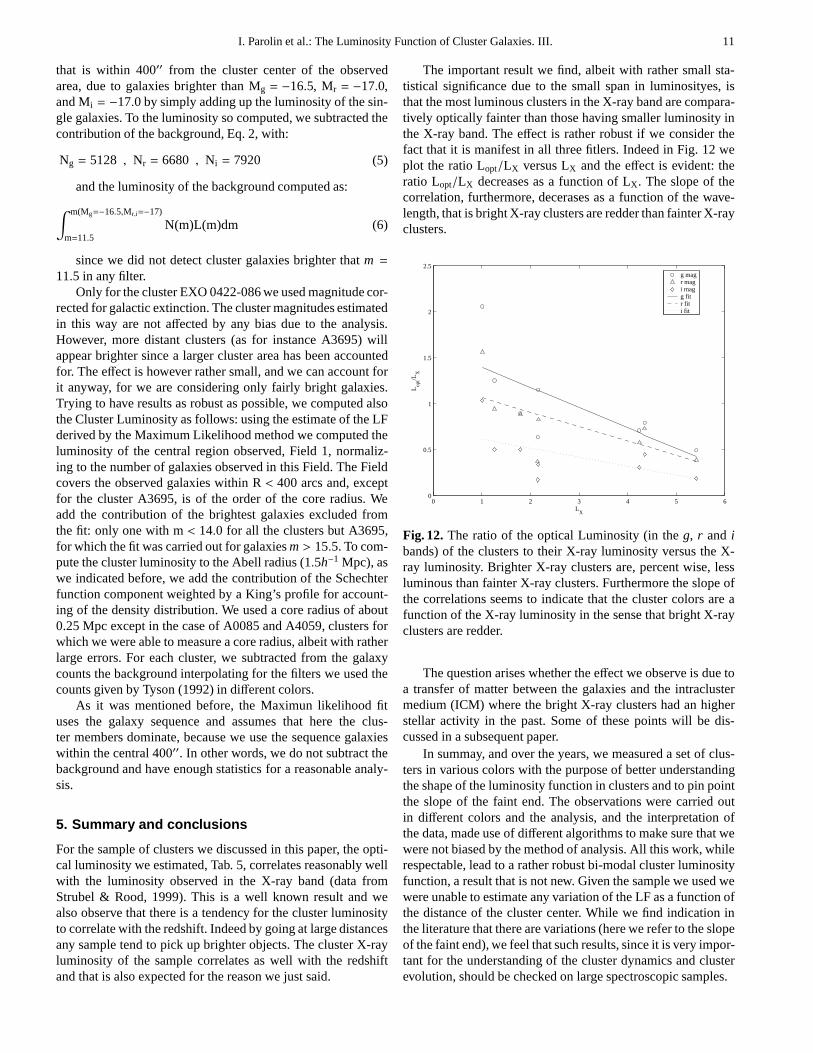
The important result we find, albeit with rather small sta-tistical significance due to the small span in luminosityes,isthat the most luminous clusters in the X-ray band are compara-tively optically fainter than those having smaller luminosity inthe X-ray band. The effect is rather robust if we consider thefact that it is manifest in all three fitlers. Indeed in Fig. 12weplot the ratio Lopt/LX versus LX and the effect is evident: theratio Lopt/LX decreases as a function of LX . The slope of thecorrelation, furthermore, decerases as a function of the wave-length, that is bright X-ray clusters are redder than fainter X-rayclusters.

0 1 2 3 4 5 60

0.5

1

1.5

2

2.5

LX

Lop

t/LX

g magr magi magg fitr fiti fit

Fig. 12. The ratio of the optical Luminosity (in theg, r and ibands) of the clusters to their X-ray luminosity versus the X-ray luminosity. Brighter X-ray clusters are, percent wise,lessluminous than fainter X-ray clusters. Furthermore the slope ofthe correlations seems to indicate that the cluster colors are afunction of the X-ray luminosity in the sense that bright X-rayclusters are redder.

The question arises whether the effect we observe is due toa transfer of matter between the galaxies and the intraclustermedium (ICM) where the bright X-ray clusters had an higherstellar activity in the past. Some of these points will be dis-cussed in a subsequent paper.

In summay, and over the years, we measured a set of clus-ters in various colors with the purpose of better understandingthe shape of the luminosity function in clusters and to pin pointthe slope of the faint end. The observations were carried outin different colors and the analysis, and the interpretation ofthe data, made use of different algorithms to make sure that wewere not biased by the method of analysis. All this work, whilerespectable, lead to a rather robust bi-modal cluster luminosityfunction, a result that is not new. Given the sample we used wewere unable to estimate any variation of the LF as a function ofthe distance of the cluster center. While we find indication inthe literature that there are variations (here we refer to the slopeof the faint end), we feel that such results, since it is very impor-tant for the understanding of the cluster dynamics and clusterevolution, should be checked on large spectroscopic samples.


The important result of this work, however, consists in theestimate of the total luminosity in different optical color and itscorrelation with the X-ray luminosity. Indeed we believe that itis the estimate of the luminosity and colors of clusters thatwillgive the opportunity, when compared to the X-ray luminosity,to better pin point some of the characteristics of the cluster andICM evolution.

Acknowledgements. We thank Alberto Moretti for the many discus-sions in the course of this work and the referee, P. Schuecker, for thehelpful suggestions.

References

Abell G. O., Corwin H. G., Olowin R. P., 1989, ApJS, 70,1Barkhouse W. A., Yee H. K. C., Lopez-Cruz O., 2002, in ASP Conf.

Ser. 268, “Tracing cosmic evolution with galaxy clusters”,ed.Borgani S., Mezzetti M., Valdarnini R., 289

Bernstein G. M., Nichol R. C., Tyson J. A., Ulmer M. P., WittmanD.,1995, AJ, 110, 1507

Binggeli B., Sandage A., Tamman G. A., 1985a, AJ, 90, 1681Binggeli B., Sandage A., Tamman G. A., 1985b,AJ, 90, 1759Binggeli B., Sandage A., Tamman G. A., 1988, ARA&A, 26, 509Biviano A., Durret F., Gerbal D. et al., 1995, A&A, 297, 610Blanton M. R., Dalcanton J., Eisenstein J., Loveday J., et al., 2001,

ApJ, 121, 2358Caldwell N., Bothun, G. D., 1987, AJ, 94, 1126Chincarini G., Rood H. J., 1972, PASP, 84, 589Chincarini G., 1988, in “Origin, structure and evolution ofgalax-

ies”, Proceedings of the Guo Shoujing School of Astrophysics,Publisher World Scientific, ed. Fang Li Zhi

Driver S. P., Phillips S., Davies J. I., Morgan I., Disney M. J., 1994,MNRAS, 268, 393

Gavazzi G., Cortese L., Boselli A. et al., 2002, submitted ApJGodwin J. G., Peach J. V., 1977, MNRAS, 181, 323Goto T., Okamura S., McKay T. A. et al., 2002, PASJ, 54, 515GImpey C., Bothun G., 1997, ARA&A, 35, 267King I. R., 1962, AJ, 67, 471Loveday J., Peterson B. A., Efstathiou G., Maddox S. J., 1992, ApJ,

390, 338Molinari E., Chincarini G., Moretti A., De Grandi S., 1998, A&A,

338,874Moretti A., 1997, Laurea Thesis, Universita degli studi diMilano, ItalyMoretti A., Molinari E., Chincarini G., De Grandi S., 1999, A&AS,

140, 155Parolin I., 2002, Laurea Thesis, Universita degli studi diMilano, ItalyRatti K., 1998, Laurea Thesis, Universita degli studi di Milano, ItalySakai S., Kennicutt R. C., van der Hulst J. M., Moss C., 2002, ApJ,

578, 842Sandage A., Binggeli B., Tamman G. A., 1985, ApJ, 90, 1759Smith R. M., Driver S. P., Phillips S., 1997, MNRAS, 287, 415SStruble M. F., Rood H. J., 1999, ApJ, 125, 35Thuan T. X.,Gunn J. E., 1976, PASP, 88, 543Tyson J. A., 1992, in “Extragalactic Background Radiation”, ed.

Calzetti D., Livio M., Madau P., Space Telescope ScienceInstitute, Symposium Series Vol 7

Visvanatan N., Sandage A., 1977, ApJ, 216, 214Wade R. A., Hoessel J.G., Elias J.H.,Huchra J.P., 1979, PASP, 91, 35Zucca et al., 1997, A&A, 326, 477


Cluster Filter G/S mG σG m∗ α

g 3.50+3.50−1.50 16.01+0.24

−0.24 0.29+0.16−0.16 15.30+0.90

−1.80 −1.59+0.04−0.04

A0085 r 3.70+4.30−2.10 15.63+0.27

−0.27 0.34+0.14−0.14 15.05+0.97

−2.80 −1.59+0.04−0.04

i 3.67+4.30−2.03 15.37+0.20

−0.20 0.33+0.16−0.16 14.44+0.60

−3.20 −1.55+0.04−0.04

g 0.81+0.27−0.27 17.07+0.18

−0.18 0.82+0.19−0.19 19.25+0.36

−0.36 −1.71+0.07−0.07

A0133 r 0.29+0.8−0.1 16.84+0.31

−0.31 0.85+0.5−0.2 19.69+0.9

−0.2 −1.34+0.17−0.17

i 0.34+0.16−0.16 16.69+0.26

−0.26 0.88+0.27−0.27 19.28+0.5

−0.2 −1.59+0.07−0.07

g 0.34+0.1−0.1 17.22+0.24

−0.24 1.04+0.23−0.23 19.23+0.30

−0.30 −1.42+0.08−0.08

A3667 r 0.16+0.04−0.04 16.66+0.31

−0.31 0.97+0.27−0.27 18.67+0.48

−0.48 −1.39+0.09−0.09

i 0.5+0.15−0.15 16.32+0.48

−0.48 1.03+0.59−0.18 18.22+0.56

−1.0 −1.52+0.07−0.07

g 0.8+0.27−0.5 18.52+0.3

−0.3 1.03+0.23−0.23 19.69+0.89

−0.89 −1.63+0.14−0.14

A3695 r 0.95+0.86−0.12 17.90+0.28

−0.28 0.93+0.20−0.20 19.16+0.62

−0.62 −1.68+0.10−0.10

i 0.38+0.09−0.09 17.88+0.32

−0.32 0.90+0.22−0.22 19.93+0.33

−0.33 −1.54+0.06−0.06

Table 3. Parameters obtained with Maximum Likelihood method and thestandard analysis


Cluster Filter G/S mG σG m∗ α

g 0.14+0.05−0.05 17.14+0.40

−0.40 1.72+0.31−0.31 21.12+0.20

−0.20 −1.39+0.07−0.07

A4038 r 0.14+0.05−0.05 16.54+0.58

−0.58 2.02+0.59−0.59 20.88+0.23

−0.23 −1.38+0.07−0.07

i 0.14+0.04−0.04 16.47+0.53

−0.53 1.86+0.49−0.49 20.86+0.19

−0.19 −1.41+0.06−0.06

g 1.16+0.70−0.70 18.20+0.84

−0.84 1.34+0.80−0.40 19.06+1.30

−1.50 −1.74+0.12−0.12

A4059 r 0.76+4.20−0.30 17.22+0.95

−0.95 1.35+1.40−0.60 18.07+1.00

−3.10 −1.65+0.70−0.10

i 1.79+4.20−0.30 16.54+3.00

−0.40 1.08+4.20−0.30 17.87+2.20

−3.50 −1.67+0.11−0.11

g 0.55+0.27−0.16 17.82+4.2

−0.76 1.64+2.13−.65 19.26+1.53

−0.42 −1.66+0.06−0.06

EXO 0422-086 r 0.43+0.20−0.20 17.46+0.24

−0.24 0.86+0.20−0.20 18.98+0.36

−0.36 −1.47+0.06−0.06

i 0.38+0.13−0.13 17.26+0.28

−0.28 0.89+0.20−0.20 18.39+0.53

−0.53 −1.40+0.07−0.07

g 0.21+0.85−0.06 17.21+0.28

−0.28 0.91+0.32−0.32 18.97+0.9

−2.0 −1.34+0.17−0.17

A0496 r 0.22+0.06−0.06 16.80+0.33

−0.33 0.98+0.31−0.31 18.31+0.6

−0.6 −1.68+0.08−0.08

i 0.78+0.71−0.36 16.46+0.21

−0.21 0.86+0.20−0.20 18.38+0.6

−1.1 −1.43+0.16−0.93

Table 4. Parameters obtained with Maximum Likelihood method and thestandard analysis


Cluster z LX Filter L0/L⊙ L0/L⊙ L0/L⊙ L0/L⊙ L/LX L/LX

1044h−2erg/s 1011h−2erg/s 1011h−2erg/s 1011h−2erg/s 1011h−2erg/s F1obs A.R.F1obs F1com 0.3Mpc A.R.

g 2.68 2.81 2.94 3.68 0.4954 0.6802A0085 0.0556 5.41 r 2.11 2.59 2.69 3.22 0.3900 0.5952

i 1.02 1.69 1.94 1.94 0.1885 0.3586g 2.49 2.84 2.86 3.01 1.1528 1.3935

A0133 0.0566 2.16 r 1.79 1.92 1.93 2.03 0.8287 0.9398i 0.74 1.13 1.14 1.18 0.326 0.5463g 3.46 3.67 3.72 3.89 0.7954 0.8943

A3667 0.0556 4.35 r 3.17 3.25 3.32 3.58 0.7287 0.8230i 1.96 2.26 2.27 2.36 0.4506 0.5425g 3.01 5.63 5.54 5.97 0.7099 1.4080

A3695 0.0893 4.24 r 2.44 6.06 5.97 6.35 0.5755 1.4976i 1.30 3.86 3.8 4.04 0.3066 0.9528g 2.08 2.83 2.84 2.86 2.0594 2.8317

A4038 0.0292 1.01 r 1.58 2.93 2.94 2.95 1.5644 2.9208i 1.05 1.09 1.09 1.09 1.0396 1.0792g 1.61 1.64 1.66 1.72 0.8994 0.9609

A4059 0.0460 1.79 r 1.59 1.75 1.76 1.80 0.8883 1.0056i 0.90 1.03 1.03 1.03 0.5028 0.5754g 1.58 1.83 1.86 1.91 1.2540 1.5159

EXO 0422-086 0.0397 1.26 r 1.19 0.91 0.92 0.96 0.9444 0.7619i 0.63 0.85 0.87 0.92 0.5000 0.7302g 1.37 1.28 1.37 1.51 0.6372 0.7023

A0496 0.0328 2.15 r 0.80 0.99 1.1 1.25 0.3721 0.5814i 0.37 0.60 0.61 0.63 0.1721 0.2930

Table 5. Luminosities obtained with the parameters of the standard analysis. X-ray luminosity computed in the 0.5− 2.0 keVband assuming a power-law spectrum with energy indexγ = 0.4 (data from Strubel & Rood 1999). NOTE: thei luminosityof A0133, A3695, A4059 and EXO 0422-086 after background correction resulted to be slightly smaller than the luminosityof the few brightest galaxies, due to a sky background overcorrection and uncertainties in the cluster counts. In these cases,the luminosity was corrected assuming that brightest galaxies are cluster members as indicated by the morphology and bytheredshift.


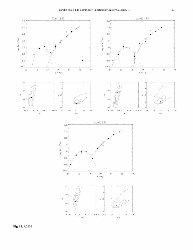
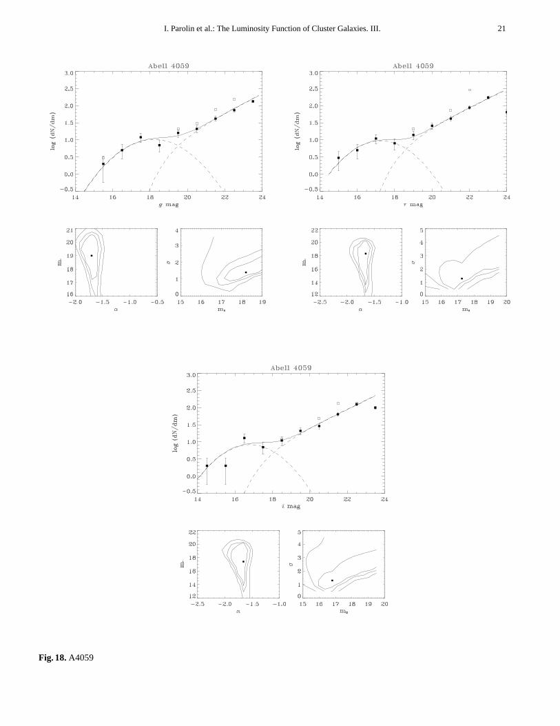
Fig. 13. Hereafter we show, for each cluster and for each filter used inthis work, the fit of our model obtained with the maximumlikelihood method and two boxes with the 1σ, 2σ and 3σ confidence contours for the parameters of the Schechter (α vs. m∗) andthe Gaussian (m0 vs.σ). In this page: A0085.


Fig. 14. A0133


Fig. 15. A3667


Fig. 16. A3695


Fig. 17. A4038


Fig. 18. A4059


Fig. 19. EXO 0422-086

The Luminosity Function of Cluster Galaxies. III. I. Parolin et al.: The Luminosity Function of...

Documents

Transcript of The Luminosity Function of Cluster Galaxies. III. I. Parolin et al.: The Luminosity Function of...