NBER WORKING PAPER SERIES

LIQUIDITY REGULATION AND UNINTENDED FINANCIAL TRANSFORMATIONIN CHINA

Kinda Cheryl HachemZheng Michael Song

Working Paper 21880http://www.nber.org/papers/w21880

NATIONAL BUREAU OF ECONOMIC RESEARCH1050 Massachusetts Avenue

Cambridge, MA 02138January 2016

An earlier draft of this paper circulated under the title "The Rise of China�s Shadow Banking System."We thank Anil Kashyap for several helpful conversations. We also thank Jeff Campbell, Doug Diamond,Chang-Tai Hsieh, John Huizinga, Randy Kroszner, Mark Kruger, Rich Rosen, Ben Sawatzky, MartinSchneider, and Harald Uhlig. Special thanks as well to Mingkang Liu and the other bankers and regulatorswe interviewed. We are also grateful to seminar and conference participants at Minnesota Carlson,CUHK, Queen�s University, Bank of Canada, Chicago Booth, Nankai, HKU, HKUST, Tsinghua, FudanUniversity, FRB Minneapolis, NUS, the 2015 Symposium on Emerging Financial Markets, SED 2015,NBER Summer Institute 2015 (Monetary Economics Workshop), FRB Chicago, and the IMF-Princeton-CUHKShenzhen Conference. Financial support from Chicago Booth and CUHK is gratefully acknowledged.The views expressed herein are those of the authors and do not necessarily reflect the views of theNational Bureau of Economic Research.

NBER working papers are circulated for discussion and comment purposes. They have not been peer-reviewed or been subject to the review by the NBER Board of Directors that accompanies officialNBER publications.

© 2016 by Kinda Cheryl Hachem and Zheng Michael Song. All rights reserved. Short sections oftext, not to exceed two paragraphs, may be quoted without explicit permission provided that full credit,including © notice, is given to the source.

Liquidity Regulation and Unintended Financial Transformation in ChinaKinda Cheryl Hachem and Zheng Michael SongNBER Working Paper No. 21880January 2016, Revised February 2016JEL No. E44,G28

ABSTRACT

China increased bank liquidity standards in the late 2000s. The interbank market became tighter andmore volatile and credit soared, contrary to expectations. To explain this, we argue that shadow bankingdeveloped among China�s small and medium-sized banks to evade the higher liquidity standards. Theshadow banks, which were not subject to interest rate ceilings on traditional bank deposits, then poacheddeposits from big commercial banks. In response, big banks used their substantial interbank marketpower to restrict credit to the shadow banks and increased their lending to non-financials. A calibrationof our unified framework generates a quantitatively important credit boom and higher and more volatileinterbank interest rates as unintended consequences of higher liquidity standards.

Kinda Cheryl HachemUniversity of ChicagoBooth School of Business5807 South Woodlawn AvenueChicago, IL 60637and NBERkinda.hachem@chicagobooth.edu

Zheng Michael SongDepartment of EconomicsChinese University of Hong KongShatin, N.T., Hong Kongzheng.michael.song@gmail.com

1 Introduction

Regulation can have unintended consequences. The challenge for economists is identifying

the channels through which these consequences arise. China’s recent experience with liq-

uidity regulation provides a puzzle and hence an opportunity to better understand some of

these channels. China began setting higher bank liquidity standards in the late 2000s. The

anticipated consequence was a more liquid interbank market and a moderation in credit.

Neither of these things happened. Instead, the interbank market became tighter and more

volatile and credit soared. This paper provides a novel explanation for what happened in

China and, in the process, sheds light on the origins of shadow banking and the unintended

consequences of financial regulation.

We start by establishing a new and comprehensive set of facts about the Chinese finan-

cial system. We then show that liquidity regulation was made counter-productive by two

economic forces: regulatory arbitrage by small banks and a response by big banks using

their interbank market power. Together, these forces generate a quantitatively important

credit boom and a tighter and more volatile interbank market as outcomes of higher liquidity

standards. Along with highlighting the importance of using micro-founded models to predict

the effect of regulation, our analysis shows that interbank market structure can re-orient the

monetary transmission mechanism, particularly in transitioning economies.

To explain the forces in our paper and how they interact, let us first explain the co-

existence of big and small banks in China’s financial system. One job of any financial system

is to connect savings with investment opportunities. In a well-functioning system, interme-

diaries identify suitable borrowers and attract enough savings to finance these borrowers by

offering savers suffi ciently high interest rates. China’s government has a long history of inter-

fering with this process by regulating interest rates. Most notably, the government imposed

an uncompetitive ceiling on deposit rates which favors banks with deep/entrenched retail

networks. State-owned banks have such networks so they have been kept big while other

banks have been kept small. Until recently, some of the distortions that could come from

this size wedge were smoothed over by the interbank market: small banks channeled almost

all of their existing deposits into non-financial loans then borrowed from big banks when in

need of extra/emergency liquidity. The big banks, flush with deposits, were willing to lend

to small banks at an appropriate rate rather than load up on additional loans to their usual

borrowers.

Things changed around 2008 when the government began enforcing a loan-to-deposit cap

which forbids banks from lending more than 75% of their deposits to non-financial firms.

2

Enforcement was complemented by a large increase in reserve requirements, making the 75%

cap akin to a liquidity standard. Big banks had loan-to-deposit ratios well below 75% so the

stricter rules were essentially aimed at small banks.

The first part of our paper shows that small banks responded by engaging in regulatory

arbitrage. In particular, small banks began offering a new savings instrument called a “wealth

management product”(WMP for short) that could be used to circumvent the regulation. As

long as the WMP does not come with an explicit principal guarantee from the issuing bank,

it does not need to be reported on the bank’s balance sheet. Instead, the savings attracted

by the WMP are funneled into a less regulated financial institution (e.g., a trust company)

which makes the loans that small banks cannot make without violating liquidity rules.1

The bank-trust cooperation just described constitutes shadow banking: it achieves the

same type of credit intermediation as a regular bank without appearing on a regulated

balance sheet. It also achieves the same type of maturity transformation as a regular bank,

with long-term assets financed by short-term liabilities (e.g., the average trust loan matures

in about two years while the average WMP matures in three months). As per Diamond and

Dybvig (1983), this mismatch creates a liquidity service for savers but is highly runnable

without government insurance.2

Among industry analysts, there is a sense that stricter liquidity rules have contributed to

shadow banking in China. However, the discussion lacks identification and exact mechanisms

have not been clearly established. Our paper exploits cross-sectional differences in WMP

issuance along with time-varying WMP characteristics to show that stricter liquidity rules

were the trigger for China’s shadow banking system. We then present a simple model which

is able to generate shadow banking as an endogenous response to regulation, corroborating

the empirical evidence.

The second part of our paper shows how to get from the shadow banking activities of

small banks to tighter interbank conditions and higher credit. To build some intuition about1That smaller banks are the driving force behind regulatory arbitrage in China stands in contrast to

other regions. In the U.S. and Europe, big banks are generally seen as the main drivers (e.g., Cetorelli andPeristiani (2012) and Acharya et al (2013)). This underscores the importance of understanding the natureof the regulations being arbitraged.

2In this regard, there is a notable similarity between unguaranteed WMPs and the asset-backed commer-cial paper vehicles that collapsed during the 2007-09 financial crisis. Another similarity is the use of implicitguarantees and/or back-up credit lines by the sponsoring bank to allay investor concerns about the riskinessof off-balance-sheet products. As a result, the products are only off-balance-sheet for accounting purposes.For more on the 2007-09 crisis, see Brunnermeier (2009), Gorton and Metrick (2012), Covitz et al (2013),Kacperczyk and Schnabl (2013), Gennaioli et al (2013), Krishnamurthy et al (2014), and the referencestherein.

3

the necessary ingredients, we start with a Walrasian interbank market where banks hit by

high liquidity shocks can borrow from banks hit by low liquidity shocks. These shocks

stem from the maturity mismatch between bank assets and liabilities. In the Walrasian

environment, the interest rate that clears the interbank market is highest when there is no

liquidity regulation. This result is the market mechanism at work. All else constant, a lower

interbank rate would prompt each individual bank to lend more outside of the interbank

market, leading to insuffi cient liquidity within the interbank market. However, once the

government introduces a liquidity minimum, banks are forced to reduce lending to meet the

minimum and, with more liquidity in the system, the interbank market clears at a lower

interest rate.3

A single yet powerful modification overturns these predictions to explain the broader

financial trends in China: introducing a big player on the interbank market. Each individual

small bank remains an interbank price-taker while the big bank is effectively a price-setter.

Liquidity regulation still leads to shadow banking by small banks but now there is competi-

tion between shadow banking and the big bank: by virtue of being off-balance-sheet, WMPs

can breach the uncompetitive ceiling on deposit rates and poach a lot of funds from the

big bank. As part of its equilibrium response, the big bank changes its interbank behavior.

Given the maturity mismatch between WMPs and trust loans, the interbank market remains

an important source of emergency liquidity for small banks. Therefore, by cutting such liq-

uidity, the big bank can make small banks less aggressive in WMP issuance and lessen the

extent to which small banks poach funds. This strategy makes the interbank market tighter

and more volatile, consistent with the data. In the interbank repo market, for example, the

weighted average interest rate increased by 50 basis points between 2007 and 2014 despite

increasing monetary injections by the central bank. The maximum daily rate also increased

by 150 basis points after 2007, reaching an unprecedented 11.6% in mid-2013. We study the

mid-2013 event using high frequency data and show that big banks as a group are indeed

manipulating the interbank market against small banks.

To recap, we argue that stricter liquidity rules pushed small banks into shadow banking

which then pushed big banks to tighten the interbank market. Our paper thus provides a

novel explanation for why China’s interbank markets became more volatile at a time when

regulatory policies were designed to increase bank liquidity. Our paper also speaks to the

large credit boom that has taken place in China. First, the reallocation of savings from

deposits at the big banks to higher-return WMPs at the small banks increases total credit

3See Farhi et al (2009) for a different environment in which a liquidity floor decreases interest rates.

4

because the small banks (and their off-balance-sheet trusts) typically lend more per unit

of savings than the big banks. Second, the strategic interbank response of the big banks

increases credit through traditional lending: rather than sitting idle on the liquidity that

they intend to withhold from the interbank market, the big banks lend more to non-financial

borrowers. Stricter liquidity rules can thus lead to more credit, not less, when one takes into

account interactions between heterogeneous banks.4

A calibration of our model generates one-third of the increase in China’s aggregate credit-

to-savings ratio between 2007 and 2014 and over one-half of the increase in interbank rates

over the same period. These are sizeable magnitudes which challenge the conventional wis-

dom that most of China’s credit boom was caused by a bank-funded fiscal stimulus package

undertaken by the central government in 2009 and 2010. A money multiplier calculation

shows that stimulus alone explains roughly the same fraction of the boom as the mecha-

nisms in our model.

The rest of the paper proceeds as follows. Section 2 describes the basic features of

China’s banking system, Section 3 presents the new empirical facts, Section 4 builds a model

to rationalize the facts, Section 5 calibrates the model, and Section 6 concludes. All proofs

are in the appendix.

2 Institutional Background

We begin with the institutional features that surround the recent transformation of China’s

financial system. We first describe the main players in the regulated banking sector (Section

2.1) and the banking regulations they face (Section 2.2). We then document how these

regulations are being circumvented (Section 2.3) and how large the resulting shadow sector

has become (Section 2.4).

2.1 Traditional Banking in China

Until the late 1970s, China had a Soviet-style financial system where the central bank was

the only bank. The Chinese government moved away from this system in the late 1970s

and early 1980s by establishing four state-owned commercial banks (the Big Four). Market-

oriented reforms initiated in the 1990s then led to two additional changes to the banking

4In this regard, our paper also contributes to the literature on the industrial organization of banking (e.g.,Corbae and D’Erasmo (2013) and the references therein).

5

system.5

First, the Big Four became much more profit-driven. All went through a major restruc-

turing in the mid-2000s and are now publicly listed. The government and the Big Four still

have close ties which limit how intensely the Big Four compete against each other (e.g., the

government holds controlling interest and appoints bank executives). However, the govern-

ment is no longer involved in decisions at the operational level. The effect of the reforms

has been striking. The average non-performing loan ratio of the Big Four fell from 30% in

2000 to roughly 2% in recent years. Combined profits also grew 19% annually from 2007 to

2014 to reach an unprecedented USD 184 billion in 2014. Individually, the banks in China’s

Big Four now constitute the first, second, fourth, and seventh largest banks in the world as

measured by total assets.6

The second notable change was entry of small and medium-sized commercial banks.

China now has twelve joint-stock commercial banks (JSCBs) operating nationally and over

two hundred city banks operating in specific regions. Many rural banks have also emerged.

The JSCBs are typically larger than the city and rural banks but all of these banks are

individually small when compared to the Big Four. For example, average deposits for the

JSCBs were only 17% of average deposits for the Big Four in 2013. As a group though,

small and medium-sized banks have chipped away at the Big Four’s deposit share. In 1995,

the Big Four held 80% of deposits in China. By 2005, they held 60%. The Big Four now

account for roughly 50% of traditional deposits.7

2.2 Banking Regulations

China’s banks are regulated by two agencies: the China Banking Regulatory Commission

(CBRC) and the People’s Bank of China (central bank). CBRC was established in 2003 to

take over banking supervision from the central bank. One part of China’s regulatory envi-

ronment, capital regulation, has been shaped by the international Basel Accords.8 However,

5These market-oriented reforms also paved the way for China’s rising private sector. For more on theprivate sector, see Hsieh and Klenow (2009), Song et al (2011), Brandt et al (2012), Lardy (2014), Hsieh andSong (2015), and the references therein.

6http://www.relbanks.com/worlds-top-banks/assets7Big state-owned firms in the industrial sector did not experience a similar post-restructuring decline in

market share.8After CBRC was established, it introduced an 8% minimum capital adequacy ratio as per Basel I.

The higher requirements of Basel III are currently being phased in. CBRC will require a minimum capitaladequacy ratio of 11.5% for systemically important banks and 10.5% for all other banks by the end of 2018.The requirements were 9.5% and 8.5% respectively at the end of 2013. For comparison, the Big Four had anaverage capital ratio of 12.7% in 2013 while the average across all Chinese banks in Bankscope was 14.7%.

6

two historically important regulations —a ceiling on bank deposit rates and a cap on bank

loan-to-deposit ratios —did not stem from similar international standards.

China has a long history of regulating deposit rates. Prior to 2004, deposit rates were

simply set by the central bank. In 2004, downward flexibility was introduced and deposit

rates were allowed to fall below the central bank’s benchmark rate. All banks stayed at the

benchmark, revealing it as a binding ceiling. Some upward flexibility was then introduced

in 2012 when the central bank allowed deposit rates of up to 1.1 times the benchmark rate.

Almost all banks for which we have systematic data responded by setting the maximum

allowable deposit rate so, once again, the central bank’s ceiling proved binding.9

The next historically important regulation, a 75% loan-to-deposit cap, was written into

China’s Law on Commercial Banks in 1995. Enforcement of the cap was loose until 2008

when CBRC moved to rein in loan growth at small and medium-sized banks. At first, CBRC

policed end-of-year loan-to-deposit ratios. It switched to end-of-quarter ratios in late 2009,

end-of-month ratios in late 2010, and average daily ratios in mid-2011. Stricter loan-to-

deposit rules were also complemented by a rapid increase in the reserve requirements set by

the central bank. Offi cial requirements were 7.5% in 2005. There was a modest increase to

9.5% by early 2007 then a rapid climb to 15.5% by February 2010. Reserve requirements

were subsequently increased twelve times to reach 21.5% by December 2011.10

2.3 Bank-Trust Cooperation as Regulatory Arbitrage

With the main banking regulations in hand, we now discuss how regulation has been circum-

vented. Wealth management products (WMPs) are the centerpiece of regulatory arbitrage in

China. A WMP is a savings instrument that is typically sold at bank counters. WMPs have

9In October 2015, China announced the removal of the deposit rate ceiling. The response of depositrates has been modest. This is consistent with (i) most interest-sensitive savings having already migrated tothe high-yielding WMPs discussed in Section 2.3 and/or (ii) on-balance-sheet deposits still entailing otherregulatory costs for banks.10We make three comments here. First, the increase in reserve requirements in 2007 was part of a policy

to sterilize the accumulation of foreign reserves without issuing central bank bills. Outstanding central bankbills peaked in 2008 and have since shrunk (Song et al (2014)). Second, the increasing frequency of CBRC’sloan-to-deposit checks between 2009 and 2011 and the complementary hikes in reserve requirements mayhave been responses to other government policies (e.g., a bank-funded stimulus package undertaken by thecentral government in 2009 and 2010). Section 3.2 (with Appendix D) will show that the stimulus alone wasnot large enough to generate a credit boom the size of China’s so we are ultimately interested in how muchof the boom can be explained by changes in bank regulation, controlling for all other government policies.The model we build in Section 4 and its calibration will help produce this counterfactual. Third, althoughChina lifted the offi cial loan-to-deposit component of its liquidity rules in late 2015, reserve requirementsremain high and loan-to-deposit restrictions can still technically be imposed via loan quotas.

7

two features which help get around the regulations discussed above. First, WMP returns

are not subject to a deposit rate ceiling. Figure 1 plots data on annualized WMP returns.

The spread relative to the one-year deposit rate has averaged 1 percentage point since 2008

and nearly 2 percentage points since 2012.11 Second, WMPs do not have to be principal-

guaranteed by the issuing bank. Without a guarantee, the WMP and the assets it invests in

are not consolidated into the bank’s balance sheet and thus not subject to loan-to-deposit

rules (or capital requirements). According to CBRC, non-guaranteed products were 70% of

total WMP issuance in 2012 and 65% of total WMP issuance in 2013.

Where do the funds from unconsolidated WMPs end up? Figure 2 shows the potential

channels. Stock, bond, and money markets are all investment options. However, at least

three pieces of evidence suggest that the key recipients of non-guaranteed WMPs are lightly-

regulated financial institutions called trust companies. First, there has been a near lockstep

evolution of trust company assets under management and WMPs outstanding (Figure 3).

Second, the funding for roughly 70% of trust assets comes from money that has already been

pooled together by other institutions, sometimes referred to as money raised through single

trust products (Figure 4). This is remarkably close to the proportion of WMPs that are not

guaranteed. Third, trust companies have responded to recent attempts at WMP regulation.

In August 2010, for example, CBRC announced that WMPs could invest at most 30% in

trust loans. The composition of trust assets then changed from 63% loans at the end of

2010Q2 to 42% loans by the end of 2011Q3.12

Another example comes in March 2013 when CBRC went even further and announced

that WMPs could invest at most 35% in non-standard debt assets (e.g., all trust assets).

Banks and trusts responded by developing the counterpart business illustrated in Figure 5.

In short, money is channeled from WMPs to trusts in two individually compliant steps. The

WMP issuer first places WMP money in another bank (or bank-affi liated off-balance-sheet

vehicle). The WMP’s return is tied to interest earned on this placement so the WMP is said

to be backed by interest rate products, not trust assets. However, trust companies appear in

the next step. In particular, they issue beneficiary rights to the recipient of the placement

who then uses the cash flows from those rights to pay the placement interest.13 We will

see in Section 3.1 that trust beneficiary rights became popular exactly when CBRC began

cracking down on direct bank-trust cooperation.

11To date, almost all WMPs have delivered above or equal to their promised returns.12Based on data from the China Trustee Association.13The recipient of the placement can acquire trust beneficiary rights either as an investment receivable or

through an “offl ine”reverse repo. Offl ine transactions are ones which do not go through the China ForeignExchange Trade System.

8

Whether direct or indirect, cooperation between banks and trust companies is important

for at least two reasons. First, it allows banks to make loans that might have otherwise vi-

olated banking regulations. Second, it involves a strong maturity mismatch. The mismatch

can be gleaned by returning to Figures 1 and 4. Figure 1 shows that WMPs are predom-

inantly short-term products. The median maturity has been around 3 months since 2008

and roughly 25% of WMPs have a maturity of 1 month or less. In contrast, Figure 4 shows

that trust companies hold the majority of their assets as loans and long-term investments.14

Further support for the long-term nature of trust company assets comes from the fact that

trusts issued products with an average maturity of 1.7 years when trying to pool money on

their own during the first half of 2013.15

2.4 Measuring the Shadow Sector

The Financial Stability Board defines shadow banking as “credit intermediation [that] takes

place in an environment where prudential regulatory standards ... are applied to a materially

lesser or different degree than is the case for regular banks engaged in similar activities”(FSB

(2011)). The cooperation between banks and trusts discussed in Section 2.3 satisfies this

definition. First, it involves maturity transformation and thus constitutes banking in the

sense of Diamond and Dybvig (1983). Second, it is funded by non-guaranteed WMPs which

are booked off-balance-sheet and away from regulatory standards. We can therefore use

non-guaranteed WMPs to get a conservative estimate of shadow banking in China. WMPs

outstanding ballooned from 2% of GDP in 2007 to nearly 25% of GDP in 2014 (Figure 3).

Also recall that roughly two-thirds of WMP issuance in 2012 and 2013 was non-guaranteed

(CBRC). We thus estimate that China’s shadow banking system grew from a negligible

fraction of GDP in 2007 to 16% of GDP in 2014.

To get a broader estimate of shadow banking, one can use the widely-cited data on total

social financing constructed by China’s National Bureau of Statistics.16 Social financing

includes bank loans, corporate bonds, equity, and other financing not accounted for by

traditional channels. Roughly one-third of other financing takes the form of undiscounted

banker’s acceptances.17 Removing these acceptances then leaves the most shadowy part of

other financing, namely loans by trust companies and entrusted firm-to-firm loans. It is an

14The sectorial composition of trust company assets has become more even over time, with infrastructureand real estate projects losing ground to industrial and commercial enterprises.15Annual Report of the Trust Industry in China (2013).16See, for example, Elliott et al (2015).17A banker’s acceptance is basically a guarantee by a bank on behalf of a depositor. More precisely, the

bank guarantees that the depositor will repay a third-party at a later date.

9

open question how much entrusted lending also involves trust companies so we group trust

and entrusted loans into one measure of shadow banking.18 By this measure, shadow banking

grew from 5% of GDP in 2007 to 24% of GDP in 2014. Notice that our conservative estimate

of shadow banking based only on bank-trust cooperation still accounts for a sizeable amount

of the broader measure.

3 Empirical Facts

This section establishes the core empirical facts that motivate our paper. Section 3.1 shows

that loan-to-deposit rules triggered shadow banking among China’s small and medium-sized

banks (henceforth SMBs). Section 3.2 documents an increase in total credit and shows

that China’s four biggest banks (the Big Four) have become more aggressive in traditional

lending. Section 3.3 shows that the Big Four are also manipulating interbank markets. Our

primary dataset is the Wind Financial Terminal which provides information about individual

wealth management products. It also provides some information about interbank conditions.

In cases where Wind is insuffi cient, we collect data from bank annual reports, regulatory

agencies, and financial association websites.

3.1 Loan-to-Deposit Ratio as Regulatory Trigger

The raw loan-to-deposit ratio across all commercial banks averaged 67% between 2007 and

2013 so the 75% cap described in Section 2 appears slack at the aggregate level. A different

story emerges from the cross-section. Figure 6 plots the loan-to-deposit ratios of the Big

Four and the joint-stock commercial banks (JSCBs).19 As a group, the JSCBs are just

satisfying the 75% cap, averaging an end-of-year loan-to-deposit ratio of 74% between 2007

and 2013. That the 75% cap is a binding constraint for the JSCBs is evidenced by the fact

that these banks have a noticeably higher loan-to-deposit ratio when the ratio is calculated

using average balances during the year rather than end-of-year balances. It is not until CBRC

increases its monitoring frequency (see Section 2.2) that the difference between the end-of-

year and average balance ratios for JSCBs begins to disappear. In contrast, the Big Four are

not constrained by the 75% cap: their loan-to-deposit ratio has been comfortably below 75%

for the past decade and there is virtually no difference between their average balance and

18Allen et al (2015) study entrusted loans made by publicly traded firms. These firms are required todisclose the loans. The authors find that public firms accounted for 10% of the total amount of entrustedloans reported by the central bank in 2013.19Historical balance sheet data for city and rural banks is spotty (particularly when it comes to average

daily balances) so these banks are excluded from Figure 6.

10

end-of-year ratios.20 We exploit this cross-sectional difference in Subsection 3.1.1. We will

then present a case study in Subsection 3.1.2 which connects changes in WMP characteristics

with changes in CBRC’s monitoring frequency to provide some time-varying evidence on the

role of loan-to-deposit rules.

3.1.1 Big Four versus Small and Medium-Sized Banks

Heterogeneity in the bindingness of the 75% cap suggests a natural test: if enforcement

of the cap did indeed trigger shadow banking, then we should see small and medium-sized

banks moving much more heavily into WMPs (and in particular off-balance-sheet WMPs)

than the Big Four. We should also see much higher holdings of trust beneficiary rights by

SMBs once CBRC restricts direct cooperation between banks and trusts. We confirm these

predictions here.

Between 2008 and 2014, SMBs accounted for 73% of all new WMP batches. The SMBs

are thus disproportionately more involved in WMP issuance than the Big Four. The SMBs

are also disproportionately more involved in non-guaranteedWMPs. Between 2008 and 2014,

SMBs issued 57% of their WMP batches without a guarantee while the Big Four issued 46%

of their WMP batches without a guarantee. The gap widens to 62% for SMBs versus 43%

for the Big Four in the second half of our sample. These estimates are based on product

counts since Wind does not yet have complete data on the total funds raised by each product.

However, using data from CBRC and the annual reports of the Big Four, we estimate that

SMBs accounted for roughly 64% of non-guaranteed WMP balances outstanding at the end

of 2013.21

Turning to trust beneficiary rights (TBRs), Figure 7 shows a dramatic rise in TBR

holdings among joint-stock banks when CBRC cracked down on bank-trust cooperation in

2013. There was no similar rise in TBR holdings among the Big Four. Figure 7 also shows

that the joint-stock banks accommodated their increase in TBR holdings by keeping fewer

balances at banks and other financial institutions (dashed black line). In other words, the

JSCBs did not sacrifice loans in order to hold TBRs. The JSCBs’substitution away from

balances at banks is also visible in the blue bars in Figure 7: both the JSCBs and the Big

20A common story is that the government uses individual loan quotas to impose even stricter limits on bigbanks. In practice though, quotas are negotiable, particularly for the Big Four who have more bargainingpower than SMBs.21The entire WMP balance in Bank of China’s annual report is described as an unconsolidated balance

yet the micro data includes several guaranteed batches for this bank that would not have matured by theend of 2013. We therefore remove Bank of China and rescale the other banks in the Big Four to back outour 64% estimate for SMBs.

11

Four have experienced decreases in balances owed to banks. However, unlike the Big Four,

the JSCBs have attracted suffi ciently more balances from non-bank financial institutions

(red bars). Off-balance-sheet vehicles that hold unguaranteed WMPs would be classified as

non-bank financial institutions. Effectively, the off-balance-sheet vehicle of one JSCB places

money with another JSCB. The other JSCB then uses returns from its TBR holdings to

pay interest on the placement. This is exactly the counterpart business discussed in Section

2.3. In principle, even more counterpart business could be occurring between the vehicles

themselves (e.g., vehicles can hold TBRs and placements can occur between vehicles).

We have now documented that shadow banking activities are dominated by SMBs.

Granger causality tests bolster this result. Using monthly detrended data on WMP batches

between January 2007 and September 2014, the null hypothesis that WMP issuance by

SMBs does not Granger-cause WMP issuance by the Big Four is rejected at 1% significance,

regardless of the detrending method or the number of lags. The opposite hypothesis that

WMP issuance by the Big Four does not Granger-cause WMP issuance by the SMBs cannot

be rejected at 10% significance. Therefore, the impetus for WMPs is indeed coming from

small and medium-sized banks. The intuition goes back to the nature of China’s banking

regulations. Recall from Section 2.2 that China has historically had a binding ceiling on

deposit rates. Such a ceiling stifles deposit rate competition and favors banks with deeper

and better-established retail networks (i.e., the Big Four). Also recall that China tightened

loan-to-deposit rules just as SMB lending was picking up. Unable to comply with the tighter

loan-to-deposit rules by attracting more deposits and unwilling to forgo profitable lending

opportunities, SMBs had the most to gain from shadow banking.

In principle, SMBs could also be using off-balance-sheet WMPs to skirt capital require-

ments. However, data from Bankscope suggests that the average SMB held more than the

minimum capital requirement even before CBRC adopted the Basel framework in 2004.

This is consistent with our discussion. In principle, banks should only want to skirt capital

requirements that force them to switch from cheap funding (deposits) to more expensive

funding (capital). However, precisely because cheap deposits are diffi cult for the average

SMB to attract, it makes sense that SMBs have traditionally had high capital ratios.

3.1.2 Case Study of China Merchants Bank

Among small and medium-sized banks, China Merchants Bank (CMB) is an important issuer

of wealth management products. In 2012, it accounted for only 3% of total banking assets

but 5.2% of WMPs outstanding at year-end and 17.7% of all WMPs issued during the

12

year.22 The time-variation in CMB’s product characteristics will provide further evidence

that WMPs are a response to loan-to-deposit rules.

It is useful to note that CMB’s loan-to-deposit ratio exhibits much the same patterns as

the aggregate JSCB ratios in Figure 6. CMB is one of the twelve joint-stock banks. CMB

averaged an end-of-year loan-to-deposit ratio of 74% between 2007 and 2013, just satisfying

the 75% cap. When calculated using average balances during the year rather than end-of-

year balances, CMB’s loan-to-deposit ratio averaged 82% over the same period. The growth

in CMB’s wealth management products has been dramatic. Annual issuance increased from

RMB 0.1 trillion in 2007 to RMB 0.7 trillion in 2008 before reaching almost RMB 5 trillion

in 2013. At the end of both 2012 and 2013, CMB had about 83% of its outstanding WMP

balances booked off-balance-sheet. Based on notes to the financial statements, figures for

earlier years were likely higher.

Count data from Wind indicates that 44% of new WMP batches issued by CMB in 2008

were backed by credit assets and notes. This figure rose to 63% in 2009, consistent with our

argument that WMPs were driven by stricter enforcement of loan-to-deposit caps.23 The

use of credit and notes as backing assets has since fallen due to CBRC’s rules on (direct)

bank-trust cooperation. CMB now backs most of its WMPs with interest rate products,

engaging in the counterpart business discussed in Section 2.3.

Further evidence on the importance of loan-to-deposit rules comes from changes in WMP

maturity. Figure 8 reveals a sizeable drop in the median maturity of CMB’s non-guaranteed

products, from just over 4 months in late 2009 to just under 1 month by mid-2011. This

drop does not occur for guaranteed WMPs nor is it matched by a drop in the promised

annualized yield on non-guaranteed products. Instead, the drop in CMB’s non-guaranteed

maturity coincides with changes in CBRC’s monitoring of loan-to-deposit ratios. Recall from

Section 2.2 that CBRC focused on the end-of-year ratio until late 2009, the end-of-quarter

ratio until late 2010, and the end-of-month ratio until mid-2011. CMB thus shortened the

maturity of its non-guaranteed products as the frequency of CBRC exams increased.

How can maturity be used to thwart more frequent exams? Upon maturity, the principal

and interest from a non-guaranteed (off-balance-sheet) WMP are automatically transferred

to the buyer’s deposit account. A buyer who wants to roll-over his investment then contacts

his bank to have the transfer reversed. In the time between the transfer and the reversal22Based on data from KPMG, CBRC, and China Merchants Bank.23The rise in credit and notes as backing assets between 2008 and 2009 also appears for small and medium-

sized banks as a whole (32% to 41%) but not for the Big Four (41% to 37%).

13

though, reserves and deposits rise, lowering the loan-to-deposit ratio observed by CBRC.24 In

the first half of 2011, CMB’s non-guaranteed products had a median maturity of just under

1 month which enables the window dressing that thwarts the end-of-month exams. To make

this point more concrete, we look at the maturity of each non-guaranteed batch relative to

its issue date. Approximately 15% of the non-guaranteed batches issued by CMB between

January 2008 and December 2010 would have matured near a month-end. This fraction

jumped to 40% in early 2011. Arbitraging on maturity became harder in mid-2011 as CBRC

began monitoring average daily ratios. Accordingly, Figure 8 shows that CMB’s median

non-guaranteed maturity has returned to roughly 3 months. The fraction of non-guaranteed

batches set to mature near a month-end has also fallen back below 20%.25

3.2 Evolution of Total Credit

We have now established that small and medium-sized banks use WMPs to get around

stricter loan-to-deposit rules. WMP issuance has grown substantially and, given the high

fraction of non-guaranteed WMPs, shadow lending by trust companies has also been able to

grow. At the same time, lending by traditional banks has grown too. Commercial banks for

which Bankscope has complete data collectively added RMB 40 trillion of new loans between

2007 and 2014, pushing the ratio of traditional lending to GDP from 75% in 2007 to 95% in

2014. Adding this to the growth of the shadow sector estimated in Section 2.4, we get a 35

percentage point increase in the ratio of total credit to GDP. This translates into a roughly

10 percentage point increase in China’s credit-to-savings ratio, which we estimate rose from

65% in 2007 to 75% in 2014.

Let us now take a closer look at the Big Four. Section 3.1 showed them to be fairly

passive in shadow banking so we are interested to see how, if at all, they have contributed to

traditional lending. One indication that the Big Four have become increasingly aggressive

in traditional lending comes from Figure 6: their loan-to-deposit ratio was falling prior to

2008 but has been rising ever since. This rise reflects both higher loan growth and lower

deposit growth. From 2005 to 2008, loans and deposits at the Big Four grew at annualized

rates of 10.9% and 14.1% respectively. From 2008 to 2014, these rates were 16.7% and 12.3%

respectively.

Why did big banks lend more aggressively against weaker deposit growth exactly when

24Keeping the automatic deposits as reserves is one approach. Another is to bring loans back on balancesheet in the form of trust beneficiary rights. The data suggest that CMB just recorded reserves between2009 and 2011.25We see similar trends for SMBs as a whole but not for the Big Four.

14

regulators began enforcing loan-to-deposit caps? A common explanation is the two-year

RMB 4 trillion stimulus package announced by China’s State Council in late 2008. Appendix

D shows that, absent the stimulus, the Big Four’s loan-to-deposit ratio would have still

increased markedly, from 0.57 in 2008 to 0.67 in 2014. This is around three-quarters of the

increase that actually happened (see Figure 6) so stimulus is an incomplete explanation of

why big banks have become less liquid. China’s overall credit boom is also not fully explained

by the stimulus package: as shown in Appendix D, stimulus explains around 40% of the 10

percentage point increase in the aggregate credit-to-savings ratio since 2007.

3.3 Price Manipulation on Interbank Markets

We argue that the main reason the Big Four have become less liquid is to tighten interbank

conditions and put pressure on the shadow banking activities of SMBs. Before formalizing

our argument, this section provides evidence that big banks can and do manipulate the

interbank market against SMBs, leading to higher and more volatile interbank interest rates.

We first document the importance of big banks on the interbank repo market.26 Wind

reports daily net positions by bank type starting in July 2009 and ending in September 2010.

We find the primary liquidity providers in this sample to be the big banks. The secondary

liquidity providers are China’s three policy banks.27 Specifically, on the 285 (out of 309)

trading days where big banks and policy banks were both net lenders, big banks were the

main net lender 93% of the time. Moreover, when big banks were the main net lender, their

net lending was 4.2 times that of policy banks. In contrast, when policy banks were the

main net lender, their net lending was only 1.6 times that of big banks. Another potentially

useful way to summarize the importance of big banks is to report the correlation between

the interbank interest rate and interbank lending by big banks versus policy banks. Figure 9

shows an upward trend in monthly average interbank interest rates since 2009 despite fairly

large monetary injections by China’s central bank. Figure 9 also shows that June 2013 was

a particularly dramatic month for interbank markets in China. We obtain transaction-level

data for June 2013 and use it in the remainder of this section.

The correlation between the overnight repo rate (ONR) and the amount lent by big banks

to JSCBs in June 2013 was -0.38. In contrast, the correlation between the ONR and the

amount lent by policy banks to JSCBs was 0.13. A similar pattern emerges for lending to

26We focus on the interbank repo market rather than the uncollateralized money market since the formeris much bigger than the latter.27The policy banks typically raise money in bond markets to fund economic development projects approved

by the central government.

15

other SMBs: the correlation between the ONR and the amount lent by big banks to other

SMBs was -0.62 while the correlation between the ONR and the amount lent by policy banks

to other SMBs was only -0.22. The much stronger (negative) correlation between interbank

lending by big banks and the interbank rate repo rate is consistent with big banks affecting

interbank conditions.

We now dig deeper into the June 2013 data to present more causal evidence about the role

played by big banks in the interbank market. Banks in general experienced some liquidity

pressure in early June 2013 as companies withdrew deposits to pay taxes and households

withdrew ahead of a statutory holiday.28 Accordingly, the weighted average interbank repo

rate rose from 4.64% on June 3 to 9.33% on June 8 before falling back down to 5.37% on

June 17. Most of the seasonal pressures seemed to have subsided yet interbank rates rose

again on June 20 after the central bank indicated it would not inject extra liquidity. The

weighted average repo rate hit 11.57%, with minimum and maximum rates of 4.1% and 30%

respectively. For comparison, the minimum and maximum rates on June 3 were 3.87% and

5.32% respectively.

The main net lenders in the interbank repo market on June 20 were the policy banks.

As discussed above, policy banks are usually not the main net lenders. The situation was

very different on June 20. Big banks were reluctant to lend (Figure 10(a)) and eager to

borrow, amassing RMB 50 billion of net borrowing by the end of the trading day. This left

policy banks as the main source of interbank liquidity. Figure 10(b) shows a sharp increase

in policy bank lending, much of which was absorbed by the big banks. This behavior by

the big banks crowded out small and medium-sized banks. For example, as shown in Figure

11, JSCBs paid a lot more for non-policy bank loans on June 20 than they did for policy

bank loans. It then stands to reason that JSCBs would have liked a higher share of policy

bank lending. Instead, they received 20% of what policy banks lent on June 20, down from

an average of 28% over the rest of the month.29 City and rural banks also faced large price

differentials between policy and non-policy bank loans. However, their share of policy bank

lending on June 20 was 22%, well below an average of 47% over the rest of the month.

Were big banks borrowing on June 20 because they really needed liquidity? Two pieces

of evidence suggest no. First, their ratio of repo lending to repo borrowing was 0.7, with

71% of the loans not directed towards other big banks or policy banks. If the Big Four were

28The Economist, “The Shibor Shock,”June 22, 2013.29For completeness, the overnight and 7 day maturities shown in Figure 11 were almost 94% of JSCB

borrowing on June 20. They were also 100% of JSCB borrowing from policy banks on this date. There wereno major differences in the haircuts imposed by policy banks versus other lenders.

16

in dire need of liquidity on June 20, we would expect to see very little outflow. Second, the

repo activities of big banks involved a maturity mismatch. Excluding transactions within

the Big Four, overnight trades accounted for 96% of big bank borrowing but only 83% of

big bank lending to non-policy banks. Roughly 80% of policy bank lending to banks outside

the Big Four was also at the overnight maturity. If big banks really needed liquidity on

June 20, we would expect the maturity of their lending to be closer to the maturity of their

borrowing. Instead, it was closer to the maturity offered by policy banks to borrower groups

that policy banks and big banks had in common.

Figure 12 shows that big banks also commanded an abnormally high interest rate spread

on June 20. In particular, their weighted average lending rate was 266 basis points above

their weighted average borrowing rate. This is high relative to other banks: city banks and

JSCBs commanded spreads of 46 and 113 basis points respectively. It is also high relative

to other days in the sample: on any other day in June 2013, the spread commanded by big

banks was between -40 and 58 basis points.

Finally, we look at dispersion in the lending rates charged by the Big Four and find

evidence of collusive pricing.30 In June 2013, the average daily coeffi cient of variation for

overnight lending rates offered by big banks was 62% of the average coeffi cient for JSCBs and

29% of the average coeffi cient for city banks. These figures were 61% and 21% respectively

on June 20. The data thus reveals more uniform pricing among big banks than among SMBs.

A common narrative is that China’s interbank market tightened on June 20 because the

central bank wanted to shock and discipline it. Our evidence challenges this narrative in

two ways. First, the policy banks were lending a lot of money at fairly low interest rates.

Given their political nature, they would not have behaved this way had the central bank

really wanted to shock the market. Second, the Big Four were manipulating the interbank

market by absorbing liquidity and intermediating it to SMBs at much higher interest rates.

This evidence also shows that the Big Four deviate from the line of the state in significant

ways. It will thus be fruitful to approach their behavior as a privately optimal choice rather

than dictum from the government.

4 A Unifying Theory of the Facts

The previous section established a set of facts about China’s banking system: (1) stricter

loan-to-deposit rules triggered shadow banking among small and medium-sized banks; (2)

30We exclude lending rates charged to policy banks given the proximity of policy banks to the government.

17

big banks have become less liquid and are manipulating the interbank market; (3) total

credit and interbank interest rates have both increased. We now build a banking model that

connects all the facts. In particular, we connect interbank manipulation by the Big Four

with shadow banking by the SMBs and show that the net effect of a tighter loan-to-deposit

cap is indeed more credit and a higher interbank rate. In other words, stricter regulation

has been entirely counter-productive.

Our model has three main ingredients: liquidity shocks, an interbank market for reserves,

and heterogeneity in interbank market power. The last ingredient is motivated by the evi-

dence in Section 3.3, namely the fact that the Big Four can change interbank prices if they so

choose. To isolate the contribution of this ingredient and expound the mechanisms behind

our quantitative results in Section 5, we proceed in steps. Section 4.1 begins by describing

an environment without heterogeneity. Section 4.2 then shows that this environment only

delivers some of the facts, namely the rise of shadow banking after stricter loan-to-deposit

rules but not the increase in total credit or the increase in interbank interest rates. Hetero-

geneity in interbank market power is introduced in Section 4.3 and shown to deliver a much

more comprehensive picture in Section 4.4.

4.1 Benchmark Model

There are three periods, t ∈ {0, 1, 2}, and a unit mass of risk neutral banks, j ∈ [0, 1]. The

economy is endowed with X > 0 units of funding. Let Xj denote the amount of funding

obtained by bank j at t = 0, where∫Xjdj = X.

Each bank can invest in a project which returns (1 + iA)2 per unit invested. Projects are

long-term, meaning that they run from t = 0 to t = 2 without the possibility of liquidation

at t = 1. However, banks are subject to short-term idiosyncratic liquidity shocks which must

be paid off at t = 1. More precisely, bank j must pay θjXj at t = 1 in order to continue

operation. The exact value of θj is drawn from a two-point distribution:

θj =

{θ` prob. π

θh prob. 1− π

where 0 < θ` < θh < 1 and π ∈ (0, 1). Each bank learns the realization of its shock in t = 1.

Prior to that, only the distribution is known.

To make the model more concrete, we can interpret the liquidity shocks through the lens

of Diamond and Dybvig (1983). In particular, banks attract funding at t = 0 by offering

18

liquidity services (e.g., deposits and/or WMPs) to owners of the funding endowment (e.g.,

households). The shock θj then represents the fraction of households that withdraw their

deposits and WMPs from bank j at t = 1.

Let us now spell out the liquidity services provided by banks. A dollar deposited at t = 0

becomes 1 + iB if withdrawn at t = 1 and (1 + iD)2 if withdrawn at t = 2. A WMP involves

the same returns plus an additional return ξj. To ease the exposition, suppose ξj only accrues

if the WMP is held until t = 2. In Diamond and Dybvig (1983), banks choose deposit rates to

achieve optimal risk-sharing for households. In China, the government essentially set deposit

rates through binding ceilings (Section 2.2). We therefore treat iB and iD as exogenous.31

Without loss of generality for the analytical results, we can then normalize iB = iD = 0 and

interpret the other interest rates in the model as spreads relative to this normalization.

Let Dj denote the funding attracted by bank j in the form of traditional deposits. The

funding attracted in the form of WMPs is Wj, with Xj ≡ Dj + Wj. In the data, deposits

and WMPs co-exist despite the fact that WMPs pay higher returns (even after potential risk

adjustments). This suggests that deposits have a convenience value which stops households

from switching entirely to WMPs. We will thus model Dj and Wj as continuous functions.

Consider for example:

Wj = ωξj (1)

Dj = X − ρ1ξj − ρ2ξ (2)

where ξ denotes the average WMP return and ω, ρ1, and ρ2 are non-negative constants. Each

individual bank takes ξ as given. A symmetric equilibrium requires ξj = ξ and Xj = X for

all j so we must impose:

ω = ρ1 + ρ2

This then allows us to write bank j’s funding share as:

Xj = X + ρ2

(ξj − ξ

)(3)

The key feature of (1) and (2) is that higher WMP returns prompt a partial substitution

from deposits to WMPs. A simple microfoundation for the specific functional forms used is

sketched in Appendix B.

31See Diamond and Kashyap (2015) for another Diamond-Dybvig environment with exogenously givendeposit rates. They motivate by saying that households have an exogenous outside option which puts a flooron deposit rates and, without competition between banks, the floor binds. In our model, the governmentjust sets the ceiling equal to the outside option.

19

We now describe how banks use their funds. The maturity mismatch between investment

projects and liquidity shocks introduces a role for reserves (i.e., savings which can be used

to pay realized liquidity shocks). The division of Xj into investment and reserves is chosen

at t = 0. Let Rj ∈ [0, Xj] denote the reserve holdings of bank j. If θj <RjXj, then bank j has

a reserve surplus at t = 1. Otherwise (θj >RjXj), it has a reserve shortage.

An interbank market exists at t = 1 to redistribute reserves across banks. The interest

rate in this market is iL. Banks are atomistic so they take iL as given when making decisions.

However, iL adjusts to clear the interbank market. Interbank lenders (borrowers) are banks

with reserve surpluses (shortages) at t = 1. Some lending may also be done by the central

bank so we introduce a supply of external funds Ψ (iL) ≡ ψiL, where ψ > 0. We focus on

symmetric equilibrium, in which case Rj and Xj are the same across banks. The condition

for interbank market clearing is then:

Rj + ψiL = θX (4)

where θ ≡ πθ` + (1− π) θh is the average liquidity shock. Total credit in this economy is the

total amount of funding invested in projects (i.e., 1−Rj).

We now allow for the possibility of a government-imposed loan limit on each bank. This

limit can also be viewed as a liquidity rule which says the ratio of reserves to on-balance-sheet

funding must be at least α ∈ (0, 1). Given the structure of our model, reserves are meant to

be used at t = 1 so enforcement of the liquidity rule is confined to t = 0. If the government

does not enforce a liquidity rule, then α = 0.

Whereas deposits must be booked on-balance-sheet, banks can choose where to manage

WMPs and the projects financed by those WMPs. If fraction τ j ∈ [0, 1] is managed in an

off-balance-sheet vehicle, then bank j’s reserve holdings only need to satisfy:

Rj ≥ α (Xj − τ jWj) (5)

The use of off-balance-sheet vehicles constitutes regulatory arbitrage.32 We can now employ

our model to study whether regulatory arbitrage is an equilibrium response to changes in

liquidity rules. To make the policy experiment concrete, suppose the government moves from

32See, for example, Adrian et al (2013) who define regulatory arbitrage as “a change in structure of activitywhich does not change the risk profile of that activity, but increases the net cash flows to the sponsor byreducing the costs of regulation.”

20

α = 0 to α = θ. Our goal here is to build intuition; Section 5 will fit the starting and ending

values of α to data.

4.2 Results for Benchmark Model

The expected profit of bank j at t = 0 is:

Υj ≡ (1 + iA)2 (Xj −Rj) + (1 + iL)Rj −[Xj + iLθXj +

(1− θ

)ξjWj

]− φ

2X2j (6)

where Wj and Xj are given by (1) and (3) respectively. The first term in (6) is revenue

from investment. The second term is potential revenue from reserves. The third term is the

bank’s expected funding cost. The fourth term is a quadratic operating cost (with φ > 0)

which will play a minimal role until Section 4.3.

The representative bank chooses the attractiveness of its WMPs ξj, the intensity of its

off-balance-sheet activities τ j ∈ [0, 1], and its reserve holdings Rj to maximize Υj subject to

the liquidity rule in (5). The Lagrange multiplier on (5) is the shadow cost of reserves. We

denote it by µj. The multipliers on τ j ≥ 0 and τ j ≤ 1 are denoted by η0j and η

1j respectively.

The first order conditions with respect to Rj, τ j, and ξj are then:

µj = (1 + iA)2 − (1 + iL) (7)

η1j = η0

j + αµjWj (8)

ξj =

(1− θ

)iL + (1− α)µj − φXj

2(1− θ

) × ρ2

ω+

αµjτ j

2(1− θ

) (9)

The first term in equation (9) captures what we will call the competitive motive for WMP

issuance. If this term is positive, then bank j wants to offer higher WMP returns in order

to attract more funding. Recall that bank j’s total funding, Xj, is given by equation (3).

Each bank takes ξ as given so increasing ξj relative to ξ increases Xj. The second term in

equation (9) captures what we will call the regulatory arbitrage motive for WMP issuance.

In the absence of a liquidity rule (α = 0), there is no regulatory arbitrage motive. There

is also no such motive when the interbank rate is high enough to make the shadow cost of

reserves (µj) zero.33

33The competitive motive can also be interpreted as a type of regulatory arbitrage, where the regulationbeing circumvented is the uncompetitive ceiling on deposit rates. Using the term “regulatory arbitrage”withreference to both liquidity rules and deposit rate rules is confusing. Since Section 3.1 showed that liquidityrules were the trigger for China’s shadow banking, we reserve the term for liquidity rules.

21

Proposition 1 Suppose φ < φ where φ is a positive threshold. If α = 0, then ξj = 0 if and

only if ρ2 = 0.

Proposition 1 establishes that there is always a competitive motive for WMP issuance

when ρ2 > 0 and operation costs are modest (φ < φ). This is because each bank perceives its

WMPs as cutting at least partly into the funding share of other banks. If ρ2 = 0, then each

bank perceives its WMPs as cutting one-for-one into its own funding share. Therefore, with

ρ2 = 0, a regulatory arbitrage motive is both necessary and suffi cient for WMP issuance. The

data show that very few WMPs were issued before CBRC’s enforcement of loan-to-deposit

caps, making the appropriate starting point either ρ2 = 0 or the combination of ρ2 > 0 and

φ ≥ φ. We start with ρ2 = 0 since it is analytically more convenient but, as will be seen

later, ρ2 > 0 with φ suffi ciently high delivers the same intuition.34

Proposition 2 Suppose ρ2 = 0. There is a unique α ∈[0, θ)such that ξj = 0 if α ≤ α and

ξj > 0 with τ j = 1 otherwise.

In words, Proposition 2 says that suffi ciently strict liquidity regulation (i.e., increasing

α above α) triggers the issuance of off-balance-sheet WMPs. The benchmark model can

therefore account for the rise of shadow banking. The incentive to issue WMPs does not come

from competition: with ρ2 = 0, the bank is simply substituting within its own liabilities.

Instead, WMPs are issued because they can be booked off-balance-sheet, away from the

binding liquidity rule.

Proposition 3 For any ρ2 ≥ 0, the interbank rate in the benchmark model is highest at

α = 0. Moving from α = 0 and ρ2 = 0 to α > 0 and ρ2 > 0 will also not generate an

increase in the interbank rate or an increase in total credit.

While the benchmark model is useful for understanding the motives behind WMP is-

suance, Proposition 3 shows that introducing a liquidity rule into this model will always lead

to a decrease in the interbank rate. Total credit (1 − Rj) must then also fall given (4).35

Proposition 3 is basically the market mechanism at work. Suppose there is no government

intervention (α = 0). At low interbank rates, price-taking banks will rely on the interbank

market for liquidity instead of holding their own reserves. In a Walrasian market, all banks

are price-takers so there will be liquidity demand at t = 1 but no liquidity supply. This

cannot be an equilibrium. Therefore, the interbank rate must be high to substitute for

government intervention.

34See Proposition 3 and Section 5.35If ψ = 0, then total credit will be constant. Either way, there cannot be a credit boom.

22

4.3 Adding Heterogeneity in Market Power

We now extend the benchmark model to include a big bank. By definition of being big, the

big bank is not an interbank price-taker.

We keep the continuum of small banks, j ∈ [0, 1], and index the big bank by k. WMP

demands are Wj = ωξj and Wk = ωξk, similar to equation (1). The funding attracted by

each bank is an augmented version of equation (3), namely:

Xj = 1− δ0 + δ1

(ξj − ξk

)+ δ2

(ξj − ξj

)(10)

Xk = δ0 + δ1

(ξk − ξj

)(11)

where ξj is the average return on small bank WMPs and total funding in the economy has

been normalized to X = 1. Small banks take ξj and ξk as given, along with being interbank

price-takers. In a symmetric equilibrium, ξj = ξj. The big bank does not take ξj as given.

Since the big bank is effectively an interbank price-setter, the interbank rate will depend

on the big bank’s realized liquidity shock. This makes the big bank’s shock an aggregate

shock so Appendix C shows that adding aggregate shocks to the benchmark model with only

small banks does not change Proposition 3.

Let isL denote the interbank rate when the big bank realizes θs, where s ∈ {`, h}. Tomake our main points, it will be enough for the big bank to affect the expected interbank

rate, ieL ≡ πi`L + (1− π) ihL. We can therefore simplify the exposition by fixing i`L = 0 and

letting ieL move with ihL.36 In Sections 4.1 and 4.2, we used market clearing to pin down the

endogenous interbank rate. We will use a similar approach here. In particular, when the big

bank gets a high liquidity shock, the condition for interbank market clearing is:

Rj +Rk + ψihL = θXj + θhXk (12)

The left-hand side captures the supply of liquidity while the right-hand side captures the

demand for liquidity.

At t = 0, the big bank’s expected profit is:

Υk ≡ (1 + iA)2 (Xk −Rk)+[1 + (1− π) ihL

]Rk−

[Xk + (1− π) ihLθhXk +

(1− θ

)ωξ2

k

]− φ

2X2k

36The proofs will verify that i`L = 0 does not result in a liquidity shortage when the big bank realizes θ`.

23

The interpretation is similar to equation (6): the first term is revenue from investment, the

second term is the expected potential revenue from reserves, the third term is the big bank’s

expected funding cost, and the fourth term is an operating cost.37

The big bank chooses Rk, τ k, and ξk to maximize Υk subject to three sets of constraints.

First are the aggregate constraints, namely funding shares as per (10) and (11) and market

clearing as per (12). Note that the market clearing equation connects Rk and ihL. Therefore,

we can think of the big bank as choosing ihL with Rk determined by (12), rather than the

other way around.

The second set of constraints comes from the first order conditions of small banks. The

representative small bank solves essentially the same problem as before. Its objective function

is still given by (6) but with (1− π) ihL as the interbank rate and Xj as per equation (10).

In the benchmark model, we used ρ2 = 0 in equation (10) to capture the empirical fact that

small banks issued virtually no WMPs at low α. The counterpart here is δ1 + δ2 = 0 in

equation (10), making the small bank first order conditions:

µj[Rj − α

(Xj − ωξj

)]= 0 with complementary slackness (13)

µj = (1 + iA)2 −[1 + (1− π) ihL

](14)

ξj =αµj

2(1− θ

) (15)

Notice that equation (15) captures essentially the same regulatory arbitrage motive as equa-

tion (9). It will be useful to deviate from the benchmark model in small steps, hence the

use of δ1 + δ2 = 0 rather than δ1 + δ2 > 0. However, we will allow for δ1 + δ2 > 0 (with

appropriate φ) in the calibration and show that the qualitative results are unchanged.

The last set of constraints on the big bank’s problem are inequality constraints, namely

the liquidity rule and non-negativity conditions:

Rk ≥ α (Xk − τ kWk)

τ k ∈ [0, 1]

ξk ≥ 0

37We are assuming the same return iA for all banks. In practice, different banks can invest in differentsectors but the “risk-adjusted”returns are roughly comparable: while the private sector is more productivethan the state sector, lending to the private sector is, at least politically, riskier. Some anecdotal evidencecan be found in Dobson and Kashyap (2006).

24

µj ≥ 0

Each inequality constraint can be in one of two cases: binding or slack. In the data, big

banks are not constrained by the liquidity rule. They are also less involved in off-balance-

sheet activities than small banks. To capture this, we will look for a solution with Rk > αXk

and τ k = 0.38 We will also require ξk = 0 at α = 0 since very few WMPs were issued before

CBRC’s enforcement of loan-to-deposit caps. Finally, we will work with µj > 0 to capture

the fact that small banks are constrained by liquidity rules.

When the big bank is unconstrained by the liquidity rule, it has no regulatory arbitrage

motive for WMP issuance. Therefore, getting ξk = 0 at α = 0 just requires disciplining any

competitive motive the big bank may have. As was the case for small banks in Proposition

1, there are two ways to do this. The first is to shut down the competitive motive altogether

(i.e., δ1 = 0). The second is to allow for a suffi ciently high operating cost (i.e., δ1 > 0 but

with φ suffi ciently positive). We will consider both cases to better understand the role that

big banks can play in this economy. The first case, δ1 = 0, implies a fixed funding share for

the big bank (i.e., Xk = δ0). The second case, δ1 > 0, makes the big bank’s funding share

endogenous. For the second case, we will set φ so that the equilibrium ξk is exactly zero at

α = 0 (as opposed to ξk being constrained by zero). We will be interested to see how, if at

all, an endogenous funding share affects the big bank’s decision-making.

4.4 Results for Extended Model

An equilibrium is characterized by the first order conditions from the small bank problem,

the first order conditions from the big bank problem, and interbank market clearing.

Proposition 4 Suppose α = 0. Set δ1 + δ2 = 0 to get ξj = 0. Also set either δ1 = 0 or

δ1 > 0 with φ suffi ciently positive to get ξk = 0. If iA lies within an intermediate range, the

equilibrium at α = 0 involves µj > 0, Rj = 0, and Rk > 0.

As in the benchmark model, a liquidity rule is not needed for the banking system to be

liquid. In contrast to the benchmark though, liquidity is now held disproportionately by the

big bank: small banks invest all their funding in projects and rely on the interbank market

to honor short-term obligations. The big bank’s willingness to hold liquidity reflects its

status as an interbank price-setter. In particular, the big bank understands that not holding

enough liquidity will increase its funding costs should it experience a high liquidity shock.38The big bank is technically indifferent between any τk ∈ [0, 1] if its rule is slack. We consider τk = 0 for

analytical convenience and because finding an equilibrium with τ j = 1 and τk = 0 will be enough to capturethe empirical fact that SMBs have a higher intensity of non-guaranteed activity.

25

We now conduct the same policy experiment as we did in the benchmark model: the

government increases the liquidity rule from α = 0 to α = θ. As discussed in Section 2,

the government’s objective could be to stifle small banks by forcing them to hold some of

their own liquidity rather than expecting liquidity from big banks. Proposition 4 established

µj > 0 at α = 0 so forcing small banks to shift from investment projects to reserves is indeed

a tax on them. As shown next, the introduction of a big bank overcomes the shortcomings

of the benchmark model and accounts for the rise in interbank rates:

Proposition 5 Keep δ1 + δ2 = 0 as in Proposition 4. The following are suffi cient for α = θ

to generate a higher interbank rate than α = 0 while preserving slackness of the big bank’s

liquidity rule, bindingness of the small bank liquidity rule (µj > 0), and feasibility of i`L = 0:

1. Suppose δ1 = 0 so that the big bank’s funding share is fixed. The suffi cient conditions

are: π suffi ciently high, θ` andψωsuffi ciently low, and iA within an intermediate range.

2. Suppose δ1 = ω > 0 so that the big bank’s funding share is endogenous. Also set φ so

that ξk is exactly zero at α = 0. The suffi cient conditions are: π suffi ciently high, θ`and ψ

ωsuffi ciently low, and iA and δ0 within intermediate ranges.

There is a non-empty set of parameters satisfying the suffi cient conditions in both 1 and 2.

All else constant, the model with an endogenous funding share generates a larger increase in

the interbank rate than the model with a fixed funding share.

To explain the content of Proposition 5, it will be useful to summarize all the forces

behind the big bank’s choice of ihL. From the big bank’s objective function:

∂Υk

∂ihL∝ Rk − θhXk︸ ︷︷ ︸

direct motive

−[

(1 + iA)2 − 1

1− π − ihL

]∂Rk

∂ihL︸ ︷︷ ︸reallocation motive

+

[(1 + iA)2 − 1− φXk

1− π − θhihL

]∂Xk

∂ihL︸ ︷︷ ︸funding share motive

(16)

The equilibrium ihL solves∂Υk∂ihL

= 0. We will first explain the three motives identified in (16).

We will then explain how these motives vary with α in order to understand why moving

from α = 0 to α = θ generates a higher interbank rate.

The first motive is what we call the direct motive. The big bank has reserves Rk and

a funding share Xk. Its net reserve position when hit by a high liquidity shock is therefore

Rk−θhXk. Each unit of reserves is valued at an interest rate of ihL when the big bank’s shock

is high so, on the margin, an increase in ihL changes the big bank’s profits by Rk − θhXk.

26

The second motive is what we call the reallocation motive. The idea is that changes in ihLalso affect how many reserves the big bank needs to hold in a market clearing equilibrium.

If ∂Rk∂ihL

< 0, then an increase ihL elicits enough liquidity from other sources to let the big bank

reallocate funding from reserves to investment. On the margin, the value of this reallocation

is the shadow cost of reserves, hence the coeffi cient on ∂Rk∂ihL

in (16). The third motive is what

we call the funding share motive. The idea is that changes in ihL also affect how much funding

the big bank attracts when funding shares are endogenous. If ∂Xk∂ihL

> 0, then an increase in

ihL curtails the WMP activities of small banks by enough to boost the big bank’s funding

share. The coeffi cient on ∂Xk∂ihL

in (16) captures the marginal value of a higher funding share

for the big bank. We will discuss this coeffi cient in more detail below.

To gain some insight into how changes in α will affect the solution to ∂Υk∂ihL

= 0 through

each motive, let’s start with the case of fixed funding shares (δ1 = 0). From market clearing:

Rk − θhXkδ1=0= θ (1− δ0)− ψihL − α

(1− δ0 −

αω (1− π)

2(1− θ

) [(1 + iA)2 − 1

1− π − ihL

])︸ ︷︷ ︸

Rj as per small bank FOCs in (13) to (15)

(17)

For a given value of ihL, the magnitude of the direct motive in (17) depends on α through the

reserve holdings of small banks. There are two competing effects. On one hand, higher α

forces small banks to hold more reserves per unit of on-balance-sheet funding. On the other

hand, higher α compels small banks to engage in regulatory arbitrage (via ξj) and move

funding off-balance-sheet. The net effect is ambiguous so we must look beyond the direct

motive to explain Proposition 5.

With fixed funding shares, the only other motive is the reallocation motive:

∂Rk

∂ihL

∣∣∣∣δ1=0

= −ψ − α2ω (1− π)

2(1− θ

) < 0 (18)

This expression is negative for two reasons. First, a higher interbank rate will attract more

external liquidity, allowing the big bank to hold fewer reserves. This is captured by the

first term in (18). Second, small banks will increase their reserves when the interbank rate

increases, also allowing the big bank to hold fewer reserves. This is captured by the second

term in (18). The effect of ihL on Rj works through the regulatory arbitrage motive of small

banks: there is less incentive to circumvent a liquidity regulation when the price of liquidity

is expected to be high. We can also see that the effect of ihL on Rj strengthens with α. This

27

is both because Rj is more responsive to changes in ξj at high α (see equation (13)) and

because ξj is more responsive to changes in ihL at high α (see equations (14) and (15)). These

results help us understand the first bullet in Proposition 5: when funding shares are fixed,

high α makes it easier for the big bank to use high interbank rates to make small banks

share the burden of keeping the system liquid.

Does the same intuition extend to the case of endogenous funding shares? No because:

∂Rk

∂ihL

∣∣∣∣δ1=ω

= −ψ +αωπ (θh − θ`) (1− π)

2(1− θ

) (19)

Higher ihL still decreases ξj but now the decrease in ξj decreases how much funding small

banks attract (Xj) and therefore how many reserves they need to hold. This effect is strong

enough to make the second term in (19) positive, in contrast to (18). We must therefore

turn to the funding share motive to explain the second bullet in Proposition 5. Note:

∂Xk

∂ihL

∣∣∣∣δ1=ω

=αω (1− π)

2(1− θ

) > 0 (20)

We already know that an increase in ihL decreases ξj which then decreases Xj. Total funding

is normalized to one so the decrease in Xj implies an increase in Xk, culminating in (20)

being positive. We also know that ξj is more responsive to ihL at high α so the magnitude of

(20) increases with α. It is therefore easier for the big bank to increase its funding share by

increasing ihL when α is high. To complete the intuition, let us reconcile the big bank’s desire

to increase its funding share when α is high with the existence of convex operating costs.

Return to the coeffi cient on ∂Xk∂ihL

in (16). All else constant, moving from α = 0 to α = θ will

trigger regulatory arbitrage by small banks. The resulting increase in ξj will erode the big

bank’s funding share, thereby decreasing the marginal operating cost φXk.

We can now understand the second bullet in Proposition 5 as follows: when funding

shares are endogenous, high α makes it easier for the big bank to use high interbank rates

to stop small banks from encroaching on its funding share. The last part of Proposition 5

establishes that sizeable increases in the interbank rate are most consistent with this sort of

asymmetric competition, wherein the big bank uses its interbank market power to fend off

competition from small banks and their off-balance-sheet activities. The next proposition

shows that our model also delivers the other empirical facts:

Proposition 6 Invoke the parameter conditions from Proposition 5 and define the loan-to-

deposit ratio as the ratio of investment to on-balance-sheet funding. Total credit increases

28

and the loan-to-deposit ratios of big and small banks converge when we move from α = 0 to

α = θ. Moreover, ξj > ξk at α = θ with ξk > 0 if and only if funding share is endogenous.

This is in contrast to ξj = ξk = 0 at α = 0.

It may now be useful to recap the intuition for our results, highlighting along the way

the channels through which total credit increases. Small banks move into off-balance-sheet

WMPs after liquidity rules tighten. Once there, they can also offer interest rates well above

the rates permitted for traditional deposits. All else constant, this poaches funding from

the big bank. Recall that the big bank internalizes the effect of reserve holdings on the

interbank market. Therefore, compared to small banks, it invests less at t = 0 per unit of

funding attracted. The reallocation of funding from deposits at the big bank to high-return

WMPs at the small banks thus increases total credit. This is one of two channels.

The second channel stems from how the big bank responds to its loss of funding. One way

for the big bank to respond is by offering its own WMPs with high interest rates. Naturally,

this is costly because of the high rates. Another way for the big bank to respond is to use

the interbank market. Small banks have less incentive to skirt liquidity rules if they expect

the price of liquidity to be high. All else constant, the interbank market at t = 1 will be

less liquid and the expected interbank rate will rise if the big bank holds fewer reserves at

t = 0. The big bank can thus manipulate the interbank market to make small banks scale

back their issuance of WMPs. While this strategy by the big bank curbs some of the initial

increase in total credit, it also boosts credit directly because the big bank shifts from reserves

to investment at t = 0. Notice that the big bank’s strategy also contributes directly to the

rise in its loan-to-deposit ratio.

5 Calibration Results

This section presents a calibration to show that the forces in our model are quantitatively

important. The starting point is 2007, just prior to China’s adoption of stricter liquidity

rules. The ending point is 2014 which is the most recent year of complete data.

We take the time from t = 0 to t = 2 to be a quarter. The average benchmark interest

rate for three-month deposits in China was 2.6% annualized so we set (1 + iD)2 = 1.026.

The benchmark demand deposit rate averaged around 0.4% so we set (1 + iB)2 = 1.004.

The average benchmark interest rate for loans with a maturity of less than six months was

5.6%. Banks can offer a discount of up to 10% on the benchmark loan rate so we set

(1 + iA)2 = 1.05.

29

The initial liquidity rule is set to α = 0.14 to match the observed loan-to-deposit ratio

of JSCBs in 2007. We use the ratio based on average balances rather than end-of-year

balances, as per Figure 6. The policy experiment is then an increase from α = 0.14 to

α = 0.25, capturing CBRC’s stricter enforcement of the 75% loan-to-deposit cap and the

complementary increase in reserve requirements.

The Big Four accounted for around 55% of all deposits in China in 2007 so we set

δ0 = 0.55. To calibrate the remaining parameters, we target moments in 2014. We can then

use the model to predict the 2007 values of these moments along with the credit-to-savings

ratio in 2007 and 2014. The competition parameters (δ1 and δ2) and the WMP demand

parameter (ω) are calibrated to match funding outcomes in 2014. We saw in Section 2.4

that WMPs were around 25% of GDP at the end of 2014. This is equivalent to 15% of

total savings. Small and medium-sized banks accounted for roughly two-thirds of WMPs

so we will target Wj = 0.10 and Wk = 0.05 for 2014. We will also target a funding share

of Xk = 0.45 for 2014 since the Big Four accounted for roughly 45% of all savings (i.e.,

traditional deposits plus WMPs) in that year.

We allow big and small banks to have different operating cost parameters, φk and φj.

China has around 200 commercial banks so a big bank is on average 40 times as large as

a small bank (i.e., 0.454/0.55

196). In the context of our model, this size difference implies that

the big bank faces φk below φj. To match the observed size difference, we set φj = 40φk so

that marginal operating costs are the same across banks.39 We then calibrate φk to match

a loan-to-deposit ratio of 0.70 for the Big Four in 2014. We will check that the resulting

operating cost parameters are high enough to deliver negligible WMP issuance in 2007.

For the low liquidity shock, the analytical results in Proposition 5 point to a small

magnitude (θ`) and a high probability (π) so we use θ` = 0 and π = 0.75. Proposition 5

also points to a low external liquidity parameter (ψ) so we use ψ = 0.5. In words, a one

percentage point increase in the interbank rate prompts a monetary injection by the central

bank of 0.5% of total savings. This is a reasonable magnitude in light of the data in Figure

9 for the period where the central bank injected liquidity.40 We will allow i`L = iB > 0 in

the calibration since surplus reserves can earn a small interest rate from the central bank.

We then redefine Ψ (iL) ≡ ψ (iL − iB) to preserve Ψ(i`L)

= 0. Lastly, we calibrate the

average liquidity shock (θ ≡ πθ` + (1− π) θh) to get an average interbank rate of 3.6% when

39Differences in φ can be interpreted as differences in retail networks that stem from exogenous social orpolitical forces. In robustness checks, we found that cutting the

φjφkratio to five (based on the size difference

between the Big Four and only the JSCBs) and re-calibrating the model generates very similar results.40Increasing ψ slightly would strengthen our main quantitative results.

30

α = 0.25. The 3.6% target is the weighted average seven-day interbank repo rate in 2014.

The seven-day rate is the longest maturity for which there is significant trading volume. It

is diffi cult to target shorter-term (e.g., overnight) repo rates since we are working with a

two-period model and each period must be long enough to match reasonable data on loan

returns (iA). This is just a level effect though: the correlation between the overnight and

seven-day repo rates is around 0.95.

The results are summarized in Table 1.41 Our model generates most of the rise in WMPs

between 2007 and 2014. It also generates half of the increase in the average seven-day

interbank repo rate. Since yearly averages can mask some of the most severe events, it is also

useful to consider the peak interbank rates observed before and after CBRC’s enforcement

action (10.1% and 11.6% respectively, as measured by daily averages). Of this 150 basis point

increase in peak rates, our model delivers 90 basis points. Returning to Table 1, the model

also delivers more than half of the decrease in the Big Four’s funding share. We also obtain

a large increase in the Big Four’s loan-to-deposit ratio, although the increase is somewhat

larger than what we observe in the data. Finally, we obtain a sizeable 3.2 percentage point

increase in the aggregate credit-to-savings ratio. This is one-third of China’s overall credit

boom and, as per Appendix D, over one-half of what is unexplained by the government’s

stimulus package.

6 Conclusion

This paper has explored the unintended consequences of a liquidity regulation and the dy-

namics of China’s shadow banking sector. We argued that shadow banking arose among

small and medium-sized banks to evade stricter liquidity rules imposed by Chinese regula-

tors. We also argued that shadow banking competes with China’s Big Four banks, prompting

the Big Four to use their interbank market power to try to impede the shadow banks. The

end result has been an increase in total credit and an increase in interbank rates, making

the stricter liquidity rules entirely counter-productive.

41The calibrated parameters are: ω = 126.84, δ1 = 266.36, δ2 = 0.374, φk = 0.0335, and θ = 0.1325.

31

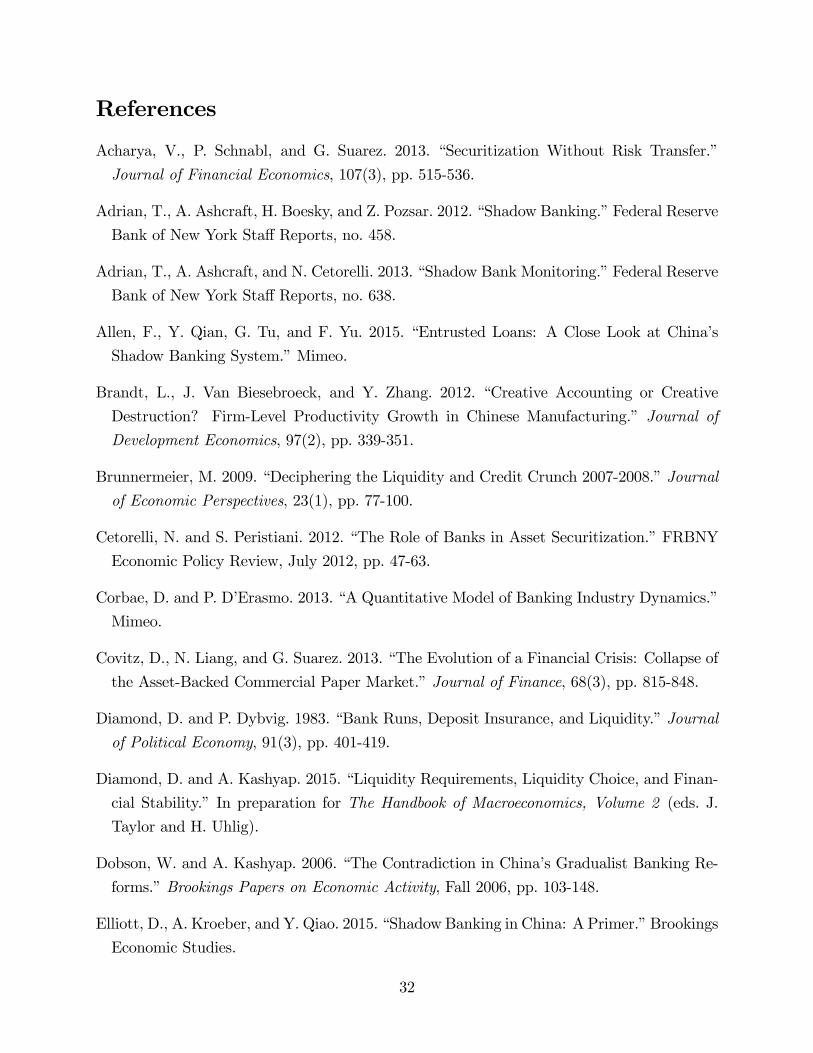
References

Acharya, V., P. Schnabl, and G. Suarez. 2013. “Securitization Without Risk Transfer.”

Journal of Financial Economics, 107(3), pp. 515-536.

Adrian, T., A. Ashcraft, H. Boesky, and Z. Pozsar. 2012. “Shadow Banking.”Federal Reserve

Bank of New York Staff Reports, no. 458.

Adrian, T., A. Ashcraft, and N. Cetorelli. 2013. “Shadow Bank Monitoring.”Federal Reserve

Bank of New York Staff Reports, no. 638.

Allen, F., Y. Qian, G. Tu, and F. Yu. 2015. “Entrusted Loans: A Close Look at China’s

Shadow Banking System.”Mimeo.

Brandt, L., J. Van Biesebroeck, and Y. Zhang. 2012. “Creative Accounting or Creative

Destruction? Firm-Level Productivity Growth in Chinese Manufacturing.” Journal of

Development Economics, 97(2), pp. 339-351.

Brunnermeier, M. 2009. “Deciphering the Liquidity and Credit Crunch 2007-2008.”Journal

of Economic Perspectives, 23(1), pp. 77-100.

Cetorelli, N. and S. Peristiani. 2012. “The Role of Banks in Asset Securitization.”FRBNY

Economic Policy Review, July 2012, pp. 47-63.

Corbae, D. and P. D’Erasmo. 2013. “A Quantitative Model of Banking Industry Dynamics.”

Mimeo.

Covitz, D., N. Liang, and G. Suarez. 2013. “The Evolution of a Financial Crisis: Collapse of

the Asset-Backed Commercial Paper Market.”Journal of Finance, 68(3), pp. 815-848.

Diamond, D. and P. Dybvig. 1983. “Bank Runs, Deposit Insurance, and Liquidity.”Journal

of Political Economy, 91(3), pp. 401-419.

Diamond, D. and A. Kashyap. 2015. “Liquidity Requirements, Liquidity Choice, and Finan-

cial Stability.” In preparation for The Handbook of Macroeconomics, Volume 2 (eds. J.

Taylor and H. Uhlig).

Dobson, W. and A. Kashyap. 2006. “The Contradiction in China’s Gradualist Banking Re-

forms.”Brookings Papers on Economic Activity, Fall 2006, pp. 103-148.

Elliott, D., A. Kroeber, and Y. Qiao. 2015. “Shadow Banking in China: A Primer.”Brookings

Economic Studies.

32

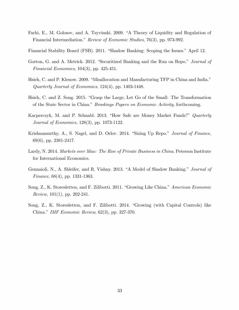
Farhi, E., M. Golosov, and A. Tsyvinski. 2009. “A Theory of Liquidity and Regulation of

Financial Intermediation.”Review of Economic Studies, 76(3), pp. 973-992.

Financial Stability Board (FSB). 2011. “Shadow Banking: Scoping the Issues.”April 12.

Gorton, G. and A. Metrick. 2012. “Securitized Banking and the Run on Repo.”Journal of

Financial Economics, 104(3), pp. 425-451.

Hsieh, C. and P. Klenow. 2009. “Misallocation and Manufacturing TFP in China and India.”

Quarterly Journal of Economics, 124(4), pp. 1403-1448.

Hsieh, C. and Z. Song. 2015. “Grasp the Large, Let Go of the Small: The Transformation

of the State Sector in China.”Brookings Papers on Economic Activity, forthcoming.

Kacperczyk, M. and P. Schnabl. 2013. “How Safe are Money Market Funds?”Quarterly

Journal of Economics, 128(3), pp. 1073-1122.

Krishnamurthy, A., S. Nagel, and D. Orlov. 2014. “Sizing Up Repo.” Journal of Finance,

69(6), pp. 2381-2417.

Lardy, N. 2014.Markets over Mao: The Rise of Private Business in China. Peterson Institute

for International Economics.

Gennaioli, N., A. Shleifer, and R. Vishny. 2013. “A Model of Shadow Banking.”Journal of

Finance, 68(4), pp. 1331-1363.

Song, Z., K. Storesletten, and F. Zilibotti. 2011. “Growing Like China.”American Economic

Review, 101(1), pp. 202-241.

Song, Z., K. Storesletten, and F. Zilibotti. 2014. “Growing (with Capital Controls) like

China.”IMF Economic Review, 62(3), pp. 327-370.

33

Figure 1

(a) Annualized WMP Returns (%, Maturity ≤ 1Yr)

Dec­07 Dec­08 Dec­09 Dec­10 Dec­11 Dec­12 Dec­130

1

2

3

4

5

6

7

8

25pmedian75pdeposit rate

(b) WMP Maturity in Months

Dec­07 Dec­08 Dec­09 Dec­10 Dec­11 Dec­12 Dec­13

mon

ths

0

5

10

15

20

25

25pmedian75p

Source: Wind Financial Terminal.

Note: Deposit rate in panel (a) is the benchmark rate for 3-month term deposits.

34

Figure 2

Anatomy of a Wealth Management Product

No GuaranteeGuaranteed

WMPBuyers

Off BalanceSheet Vehicle

Bond & MM

Stock MarketOn Balance

Sheet

TrustCompany

Property

Industry

Infrastructure

Other

Bank A

Figure 3

Source: PBOC, CBRC, IMF, China Trustee Association, KPMG China Trust Surveys

35

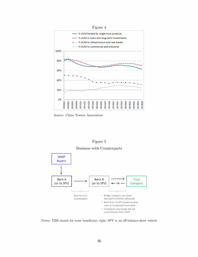
Figure 4

Source: China Trustee Association

Figure 5

Business with Counterparts

Notes: TBR stands for trust beneficiary right; SPV is an off-balance-sheet vehicle

36

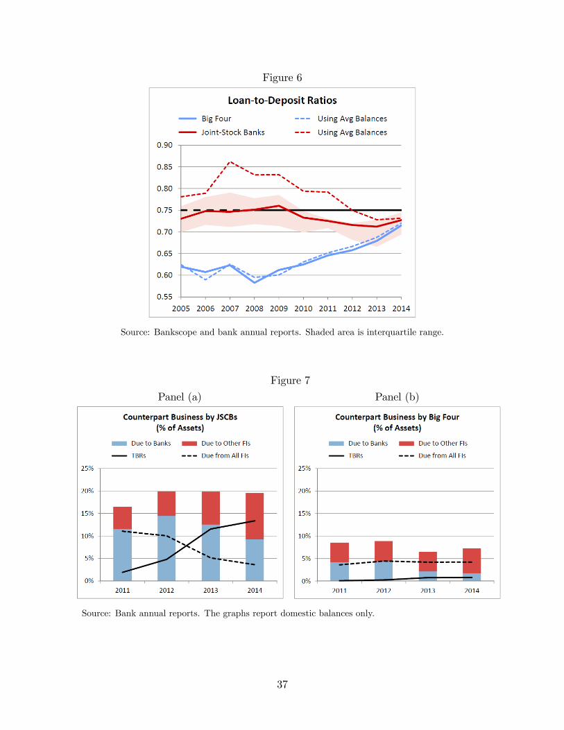
Figure 6

Source: Bankscope and bank annual reports. Shaded area is interquartile range.

Figure 7

Panel (a) Panel (b)

Source: Bank annual reports. The graphs report domestic balances only.

37

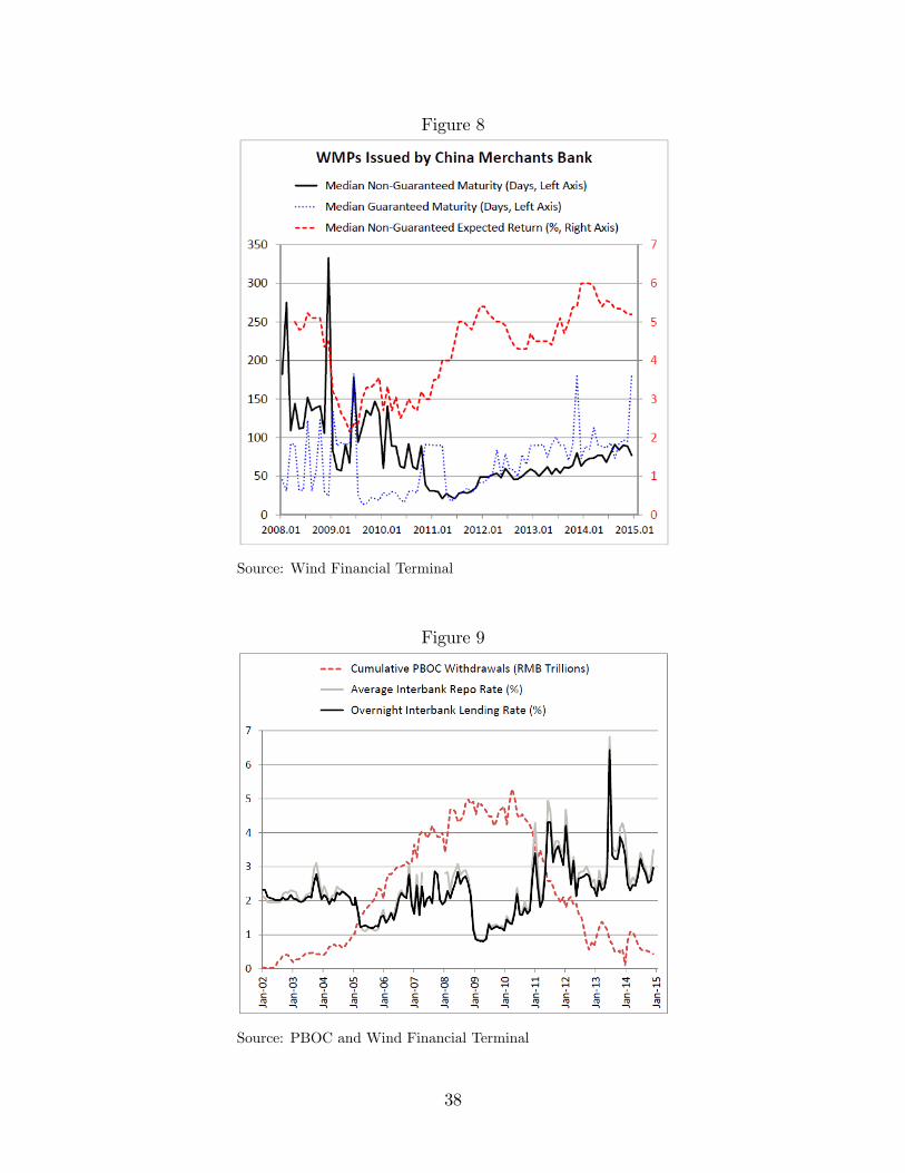
Figure 8

Source: Wind Financial Terminal

Figure 9

Source: PBOC and Wind Financial Terminal

38

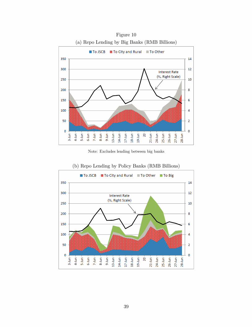
Figure 10

(a) Repo Lending by Big Banks (RMB Billions)

Note: Excludes lending between big banks

(b) Repo Lending by Policy Banks (RMB Billions)

39

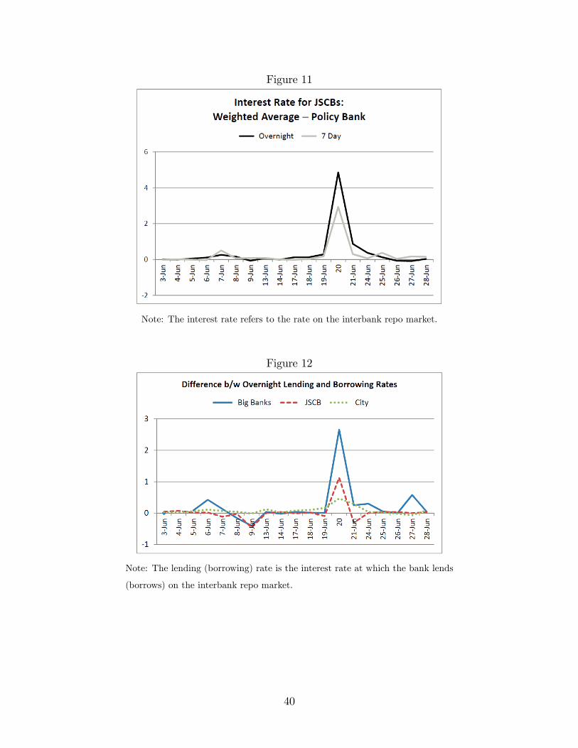
Figure 11

Note: The interest rate refers to the rate on the interbank repo market.

Figure 12

Note: The lending (borrowing) rate is the interest rate at which the bank lends

(borrows) on the interbank repo market.

40

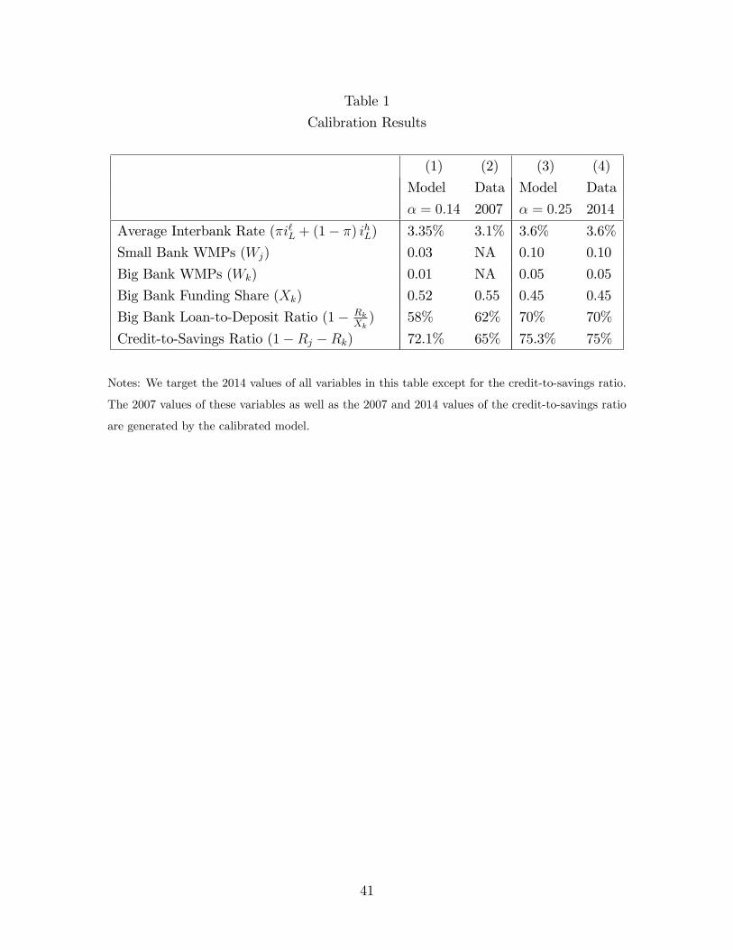
Table 1

Calibration Results

(1) (2) (3) (4)

Model Data Model Data

α = 0.14 2007 α = 0.25 2014

Average Interbank Rate (πi`L + (1− π) ihL) 3.35% 3.1% 3.6% 3.6%

Small Bank WMPs (Wj) 0.03 NA 0.10 0.10

Big Bank WMPs (Wk) 0.01 NA 0.05 0.05

Big Bank Funding Share (Xk) 0.52 0.55 0.45 0.45

Big Bank Loan-to-Deposit Ratio (1− RkXk) 58% 62% 70% 70%

Credit-to-Savings Ratio (1−Rj −Rk) 72.1% 65% 75.3% 75%

Notes: We target the 2014 values of all variables in this table except for the credit-to-savings ratio.

The 2007 values of these variables as well as the 2007 and 2014 values of the credit-to-savings ratio

are generated by the calibrated model.

41

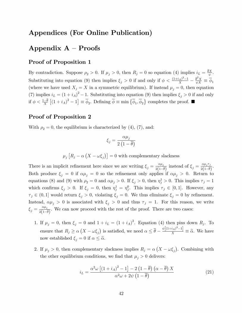
Appendices (For Online Publication)

Appendix A —Proofs

Proof of Proposition 1

By contradiction. Suppose ρ2 > 0. If µj > 0, then Rj = 0 so equation (4) implies iL = θXψ.

Substituting into equation (9) then implies ξj > 0 if and only if φ < (1+iA)2−1X

− θ2X

ψX≡ φ1

(where we have used Xj = X in a symmetric equilibrium). If instead µj = 0, then equation

(7) implies iL = (1 + iA)2− 1. Substituting into equation (9) then implies ξj > 0 if and only

if φ < 1−θX

[(1 + iA)2 − 1

]≡ φ2. Defining φ ≡ min

{φ1, φ2

}completes the proof. �

Proof of Proposition 2

With ρ2 = 0, the equilibrium is characterized by (4), (7), and:

ξj =αµj

2(1− θ

)µj[Rj − α

(X − ωξj

)]= 0 with complementary slackness

There is an implicit refinement here since we are writing ξj =αµj

2(1−θ)instead of ξj =

αµjτ j

2(1−θ).

Both produce ξj = 0 if αµj = 0 so the refinement only applies if αµj > 0. Return to

equations (8) and (9) with ρ2 = 0 and αµj > 0. If ξj > 0, then η1j > 0. This implies τ j = 1

which confirms ξj > 0. If ξj = 0, then η1j = η0

j . This implies τ j ∈ [0, 1]. However, any

τ j ∈ (0, 1] would return ξj > 0, violating ξj = 0. We thus eliminate ξj = 0 by refinement.

Instead, αµj > 0 is associated with ξj > 0 and thus τ j = 1. For this reason, we write

ξj =αµj

2(1−θ). We can now proceed with the rest of the proof. There are two cases:

1. If µj = 0, then ξj = 0 and 1 + iL = (1 + iA)2. Equation (4) then pins down Rj. To

ensure that Rj ≥ α(X − ωξj

)is satisfied, we need α ≤ θ − ψ[(1+iA)2−1]

X≡ α̃. We have

now established ξj = 0 if α ≤ α̃.

2. If µj > 0, then complementary slackness implies Rj = α(X − ωξj

). Combining with

the other equilibrium conditions, we find that µj > 0 delivers:

iL =α2ω

[(1 + iA)2 − 1

]− 2

(1− θ

) (α− θ

)X

α2ω + 2ψ(1− θ

) (21)

42

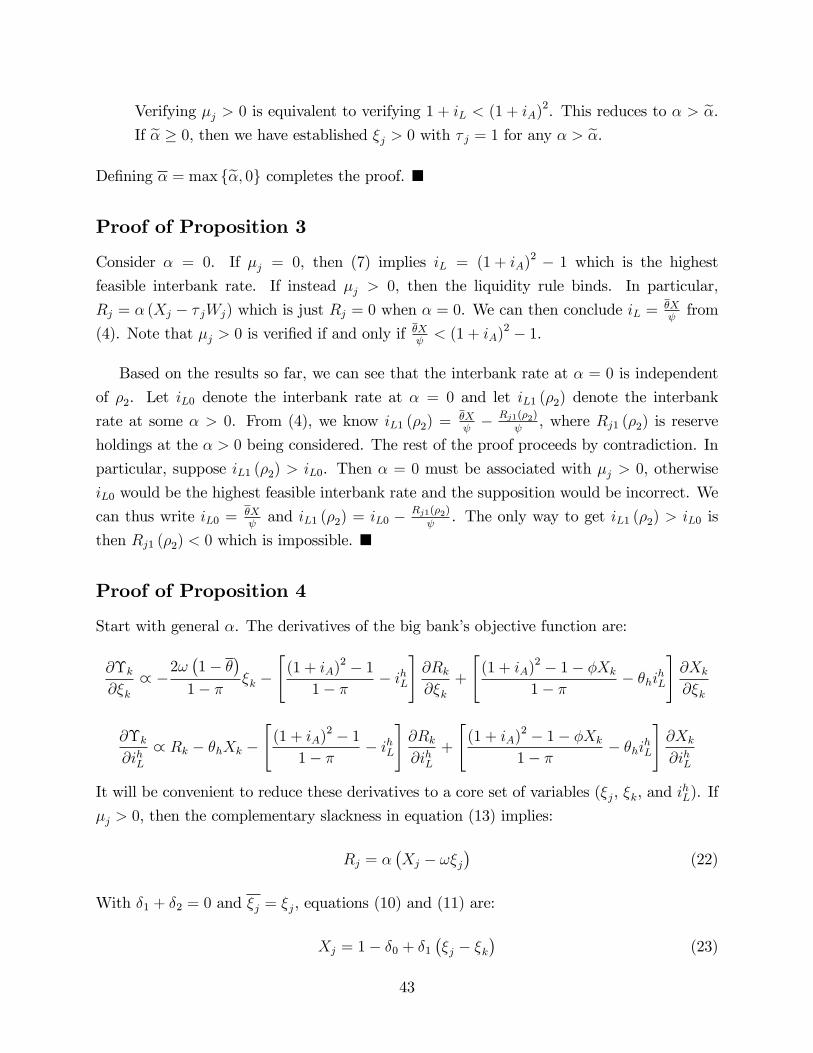
Verifying µj > 0 is equivalent to verifying 1 + iL < (1 + iA)2. This reduces to α > α̃.

If α̃ ≥ 0, then we have established ξj > 0 with τ j = 1 for any α > α̃.

Defining α = max {α̃, 0} completes the proof. �

Proof of Proposition 3

Consider α = 0. If µj = 0, then (7) implies iL = (1 + iA)2 − 1 which is the highest

feasible interbank rate. If instead µj > 0, then the liquidity rule binds. In particular,

Rj = α (Xj − τ jWj) which is just Rj = 0 when α = 0. We can then conclude iL = θXψfrom

(4). Note that µj > 0 is verified if and only if θXψ< (1 + iA)2 − 1.

Based on the results so far, we can see that the interbank rate at α = 0 is independent

of ρ2. Let iL0 denote the interbank rate at α = 0 and let iL1 (ρ2) denote the interbank

rate at some α > 0. From (4), we know iL1 (ρ2) = θXψ− Rj1(ρ2)

ψ, where Rj1 (ρ2) is reserve

holdings at the α > 0 being considered. The rest of the proof proceeds by contradiction. In

particular, suppose iL1 (ρ2) > iL0. Then α = 0 must be associated with µj > 0, otherwise

iL0 would be the highest feasible interbank rate and the supposition would be incorrect. We

can thus write iL0 = θXψand iL1 (ρ2) = iL0 − Rj1(ρ2)

ψ. The only way to get iL1 (ρ2) > iL0 is

then Rj1 (ρ2) < 0 which is impossible. �

Proof of Proposition 4

Start with general α. The derivatives of the big bank’s objective function are:

∂Υk

∂ξk∝ −

2ω(1− θ

)1− π ξk −

[(1 + iA)2 − 1

1− π − ihL

]∂Rk

∂ξk+

[(1 + iA)2 − 1− φXk

1− π − θhihL

]∂Xk

∂ξk

∂Υk

∂ihL∝ Rk − θhXk −

[(1 + iA)2 − 1

1− π − ihL

]∂Rk

∂ihL+

[(1 + iA)2 − 1− φXk

1− π − θhihL

]∂Xk

∂ihL

It will be convenient to reduce these derivatives to a core set of variables (ξj, ξk, and ihL). If

µj > 0, then the complementary slackness in equation (13) implies:

Rj = α(Xj − ωξj

)(22)

With δ1 + δ2 = 0 and ξj = ξj, equations (10) and (11) are:

Xj = 1− δ0 + δ1

(ξj − ξk

)(23)

43

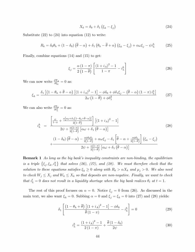
Xk = δ0 + δ1

(ξk − ξj

)(24)

Substitute (22) to (24) into equation (12) to write:

Rk = δ0θh + (1− δ0)(θ − α

)+ δ1

(θh − θ + α

) (ξk − ξj

)+ αωξj − ψihL (25)

Finally, combine equations (14) and (15) to get:

ξj =α (1− π)

2(1− θ

) [(1 + iA)2 − 1

1− π − ihL

](26)

We can now write ∂Υk∂ξk

= 0 as:

ξk =δ1

[(1− θh + θ − α

) [(1 + iA)2 − 1

]− φδ0 + φδ1ξj −

(θ − α

)(1− π) ihL

]2ω(1− θ

)+ φδ2

1

(27)

We can also write ∂Υk∂ihL

= 0 as:

ihL =

[ψ

1−π +α[αω+δ1(1−θh+θ−α)]

2(1−θ)

] [(1 + iA)2 − 1

]2ψ + α(1−π)

2(1−θ)

[αω + δ1

(θ − α

)] (28)

+

(1− δ0)(θ − α

)− αφδ0δ1

2(1−θ)+ αωξj − δ1

[θ − α + αφδ1

2(1−θ)

] (ξk − ξj

)2ψ + α(1−π)

2(1−θ)

[αω + δ1

(θ − α

)]Remark 1 As long as the big bank’s inequality constraints are non-binding, the equilibriumis a triple

{ξj, ξk, i

hL

}that solves (26), (27), and (28). We must therefore check that the

solution to these equations satisfies ξk ≥ 0 along with Rk > αXk and µj > 0. We also need

to check Wj ≤ Xj and Wk ≤ Xk so that deposits are non-negative. Finally, we want to check

that i`L = 0 does not result in a liquidity shortage when the big bank realizes θ` at t = 1.

The rest of this proof focuses on α = 0. Notice ξj = 0 from (26). As discussed in the

main text, we also want ξk = 0. Subbing α = 0 and ξj = ξk = 0 into (27) and (28) yields:

δ1

[(1− θh + θ

) [(1 + iA)2 − 1

]− φδ0

θ (1− π)− ihL

]= 0 (29)

ihL =(1 + iA)2 − 1

2 (1− π)+θ (1− δ0)

2ψ(30)

44

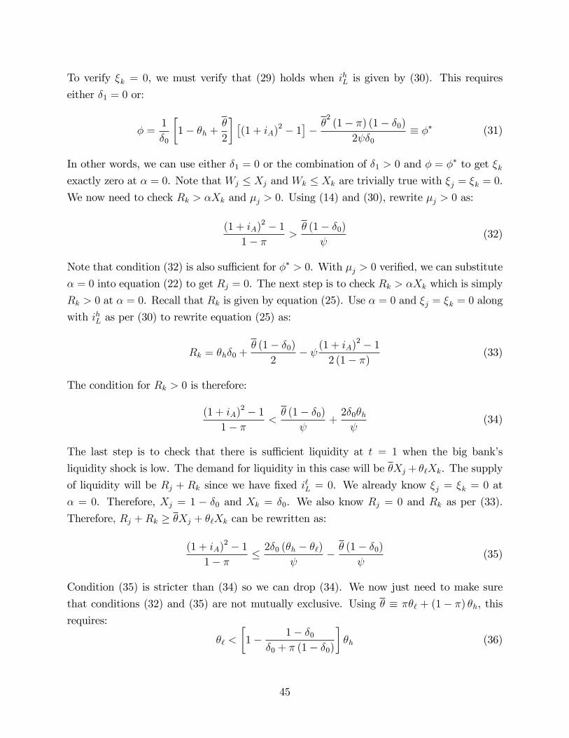
To verify ξk = 0, we must verify that (29) holds when ihL is given by (30). This requires

either δ1 = 0 or:

φ =1

δ0

[1− θh +

θ

2

] [(1 + iA)2 − 1

]− θ

2(1− π) (1− δ0)

2ψδ0

≡ φ∗ (31)

In other words, we can use either δ1 = 0 or the combination of δ1 > 0 and φ = φ∗ to get ξkexactly zero at α = 0. Note that Wj ≤ Xj and Wk ≤ Xk are trivially true with ξj = ξk = 0.

We now need to check Rk > αXk and µj > 0. Using (14) and (30), rewrite µj > 0 as:

(1 + iA)2 − 1

1− π >θ (1− δ0)

ψ(32)

Note that condition (32) is also suffi cient for φ∗ > 0. With µj > 0 verified, we can substitute

α = 0 into equation (22) to get Rj = 0. The next step is to check Rk > αXk which is simply

Rk > 0 at α = 0. Recall that Rk is given by equation (25). Use α = 0 and ξj = ξk = 0 along

with ihL as per (30) to rewrite equation (25) as:

Rk = θhδ0 +θ (1− δ0)

2− ψ (1 + iA)2 − 1

2 (1− π)(33)

The condition for Rk > 0 is therefore:

(1 + iA)2 − 1

1− π <θ (1− δ0)

ψ+

2δ0θhψ

(34)

The last step is to check that there is suffi cient liquidity at t = 1 when the big bank’s

liquidity shock is low. The demand for liquidity in this case will be θXj + θ`Xk. The supply

of liquidity will be Rj + Rk since we have fixed i`L = 0. We already know ξj = ξk = 0 at

α = 0. Therefore, Xj = 1 − δ0 and Xk = δ0. We also know Rj = 0 and Rk as per (33).

Therefore, Rj +Rk ≥ θXj + θ`Xk can be rewritten as:

(1 + iA)2 − 1

1− π ≤ 2δ0 (θh − θ`)ψ

− θ (1− δ0)

ψ(35)

Condition (35) is stricter than (34) so we can drop (34). We now just need to make sure

that conditions (32) and (35) are not mutually exclusive. Using θ ≡ πθ` + (1− π) θh, this

requires:

θ` <

[1− 1− δ0

δ0 + π (1− δ0)

]θh (36)

45

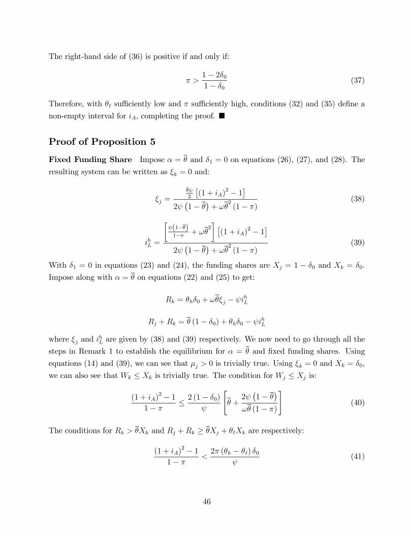
The right-hand side of (36) is positive if and only if:

π >1− 2δ0

1− δ0

(37)

Therefore, with θ` suffi ciently low and π suffi ciently high, conditions (32) and (35) define a

non-empty interval for iA, completing the proof. �

Proof of Proposition 5

Fixed Funding Share Impose α = θ and δ1 = 0 on equations (26), (27), and (28). The

resulting system can be written as ξk = 0 and:

ξj =θψ2

[(1 + iA)2 − 1

]2ψ(1− θ

)+ ωθ

2(1− π)

(38)

ihL =

[ψ(1−θ)

1−π + ωθ2] [

(1 + iA)2 − 1]

2ψ(1− θ

)+ ωθ

2(1− π)

(39)

With δ1 = 0 in equations (23) and (24), the funding shares are Xj = 1 − δ0 and Xk = δ0.

Impose along with α = θ on equations (22) and (25) to get:

Rk = θhδ0 + ωθξj − ψihL

Rj +Rk = θ (1− δ0) + θhδ0 − ψihL

where ξj and ihL are given by (38) and (39) respectively. We now need to go through all the

steps in Remark 1 to establish the equilibrium for α = θ and fixed funding shares. Using

equations (14) and (39), we can see that µj > 0 is trivially true. Using ξk = 0 and Xk = δ0,

we can also see that Wk ≤ Xk is trivially true. The condition for Wj ≤ Xj is:

(1 + iA)2 − 1

1− π ≤ 2 (1− δ0)

ψ

[θ +

2ψ(1− θ

)ωθ (1− π)

](40)

The conditions for Rk > θXk and Rj +Rk ≥ θXj + θ`Xk are respectively:

(1 + iA)2 − 1

1− π <2π (θh − θ`) δ0

ψ(41)

46

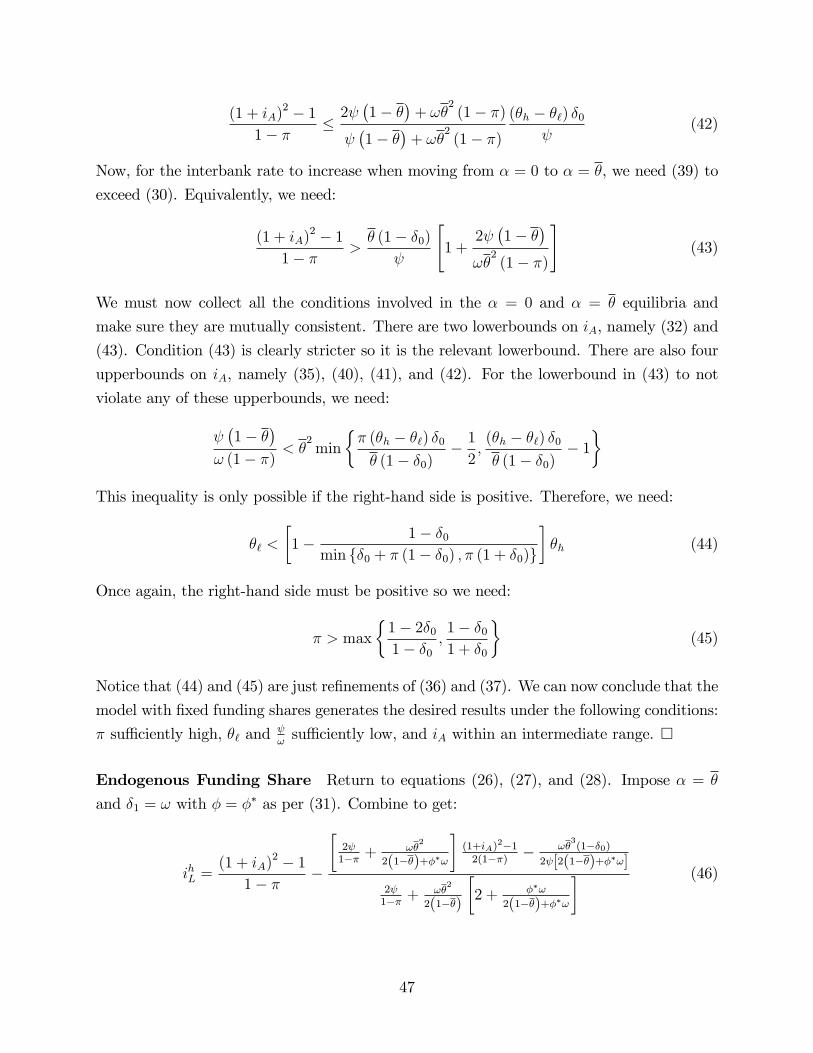
(1 + iA)2 − 1

1− π ≤2ψ(1− θ

)+ ωθ

2(1− π)

ψ(1− θ

)+ ωθ

2(1− π)

(θh − θ`) δ0

ψ(42)

Now, for the interbank rate to increase when moving from α = 0 to α = θ, we need (39) to

exceed (30). Equivalently, we need:

(1 + iA)2 − 1

1− π >θ (1− δ0)

ψ

[1 +

2ψ(1− θ

)ωθ

2(1− π)

](43)

We must now collect all the conditions involved in the α = 0 and α = θ equilibria and

make sure they are mutually consistent. There are two lowerbounds on iA, namely (32) and

(43). Condition (43) is clearly stricter so it is the relevant lowerbound. There are also four

upperbounds on iA, namely (35), (40), (41), and (42). For the lowerbound in (43) to not

violate any of these upperbounds, we need:

ψ(1− θ

)ω (1− π)

< θ2

min

{π (θh − θ`) δ0

θ (1− δ0)− 1

2,(θh − θ`) δ0

θ (1− δ0)− 1

}This inequality is only possible if the right-hand side is positive. Therefore, we need:

θ` <

[1− 1− δ0

min {δ0 + π (1− δ0) , π (1 + δ0)}

]θh (44)

Once again, the right-hand side must be positive so we need:

π > max

{1− 2δ0

1− δ0

,1− δ0

1 + δ0

}(45)

Notice that (44) and (45) are just refinements of (36) and (37). We can now conclude that the

model with fixed funding shares generates the desired results under the following conditions:

π suffi ciently high, θ` andψωsuffi ciently low, and iA within an intermediate range. �

Endogenous Funding Share Return to equations (26), (27), and (28). Impose α = θ

and δ1 = ω with φ = φ∗ as per (31). Combine to get:

ihL =(1 + iA)2 − 1

1− π −

[2ψ

1−π + ωθ2

2(1−θ)+φ∗ω

](1+iA)2−1

2(1−π)− ωθ

3(1−δ0)

2ψ[2(1−θ)+φ∗ω]

2ψ1−π + ωθ

2

2(1−θ)

[2 + φ∗ω

2(1−θ)+φ∗ω

] (46)

47

ξk =

θ(1−π)2

[θ(1−δ0)

ψ+(φ∗ω1−θ − 1

)(1+iA)2−1

1−π − φ∗ω1−θ i

hL

]2(1− θ

)+ φ∗ω

(47)

We now need to go through the steps in Remark 1 to establish the equilibrium for α = θ

and endogenous funding shares. The expressions here are more complicated so we proceed

by finding one value of iA that satisfies all the steps in Remark 1. A continuity argument

will then allow us to conclude that all the steps are satisfied for a non-empty range of iA.

Consider iA such that:(1 + iA)2 − 1

1− π =θ

ψ(48)

Substituting into (31) then pins down φ∗ as:

φ∗ =θ (1− π)

ψ

[1− θhδ0

+θ

2

](49)

From the proof of Proposition 4, we already have (32) and (35) as restrictions on iA. We

also have (36) as an upperbound on θ` and (37) as a lowerbound on π. It is easy to see that

iA as defined in (48) satisfies (32). For (48) to also satisfy (35), we need:

θ` <

[1− 2− δ0

2δ0 + π (2− δ0)

]θh (50)

π >2− 3δ0

2− δ0

(51)

Conditions (50) and (51) are stricter than (36) and (37). We can thus drop (36) and (37).

The first step is to verify µj > 0. Use (14) and (46) to write µj > 0 as:

(1 + iA)2 − 1

1− π

[1 +

2ψ[2(1− θ

)+ φ∗ω

]ωθ

2(1− π)

]>θ (1− δ0)

ψ

This is true by condition (32).

The second step is to verify ξk > 0. Substituting (46) into (47), we see that we need:

(1 + iA)2 − 1

1− π

1− φ∗

2(1−θ)ω

+ θ2(1−π)ψ

< θ (1− δ0)

ψ(52)

48

Using iA as per (48) and φ∗ as per (49):

ψ(1− θ

)ω (1− π)

<θ

2δ20

[1− θh − θδ0

(δ0 −

1

2

)]︸ ︷︷ ︸

call this Z1

(53)

If Z1 > 0, then (53) requires ψωsuffi ciently low. Note that Z1 > 0 can be made true for

any δ0 ∈ (0, 1) by assuming θ < 2 (1− θh) or, equivalently, θ` < 2−(3−π)θhπ

. This is another

positive ceiling on θ` provided π > 3− 2θh.

The third step is to verify Rk > θXk. Use α = θ and δ1 = ω to rewrite (24) and (25) as:

Xk = δ0 + ω(ξk − ξj

)(54)

Rk = δ0θh + ωθhξk − ω(θh − θ

)ξj − ψihL (55)

Therefore, Rk > θXk requires:

ihL <δ0

(θh − θ

)ψ

+ω(θh − θ

)ψ

(ξk − ξj

)+ωθ

ψξj

Use (47) to replace ξk and (26) with α = θ to replace ξj:[1 +

ωθ (1− π)

2ψ(1− θ

) [θ − 2(1− θ

) (θh − θ

)2(1− θ

)+ φ∗ω

]]ihL

<θh − θψ

[δ0 +

ωθ2

(1− π) (1− δ0)

2ψ[2(1− θ

)+ φ∗ω

]]− ωθ[(1 + iA)2 − 1

]2ψ

[3(θh − θ

)2(1− θ

)+ φ∗ω

− θ

1− θ

]

Now use (46) to replace ihL and rearrange to isolate iA:

(1 + iA)2 − 1

1− π

[2θh −

3θ

2+

2ψ(1− θ

)ωθ (1− π)

+ωθ

2(1− π)

4ψ(1− θ

) (3θh − 4θ)

+φ∗

θ

[ωθ

2

1− θ+

ψ

1− π

]]

<

[2δ0

(θh − θ

)1− π

2(1− θ

)+ φ∗ω

ωθ− θ

2(1− δ0)

2ψ

][1 +

θ2

2

ω (1− π)

ψ(1− θ

)]

+(θh − θ

) θψ

[ωφ∗δ0

2(1− θ

) + (1− δ0)

[1 +

3θ2

4

ω (1− π)

ψ(1− θ

)]]

We can simplify a bit further by using (31) to replace all instances of φ∗δ0 then grouping

49

like terms:

(1 + iA)2 − 1

1− π

θh − θ2

+2ψ(1−θ)ωθ(1−π)

− ωθ3(1−π)

4ψ(1−θ)+ φ∗

θ

[ωθ

2

1−θ + ψ1−π

]−(θh − θ

)(1− θh)

[2θ

+ 3θ2ω(1−π)

ψ(1−θ)

]

<

[4δ0

(1− θ

) (θh − θ

)ωθ (1− π)

− θ2

(1− δ0)

2ψ

][1 +

θ2

2

ω (1− π)

ψ(1− θ

)]

Substitute iA as per (48) and φ∗ as per (49) then rearrange:

ψ(1− θ

)ω (1− π)

[θh −

θ (1 + δ0)

2+

[θ +

1− θhδ0

+2

θ

ψ(1− θ

)ω (1− π)

][1−

2δ0

(θh − θ

)θ

]](56)

<θ

δ0

[θ

2δ2

0

4+δ0

2

[3(θh − θ

)(1− θh)− θ

2]− θ (1− θh)

]︸ ︷︷ ︸

call this Z2

Condition (56) will be true for ψωsuffi ciently low if Z2 > 0. Use θ ≡ πθ` + (1− π) θh to

rewrite Z2 > 0 as:

π2 (θh − θ`)2 − 2

[θh +

(2 + 3δ0) (1− θh)δ0 (2− δ0)

]π (θh − θ`) + θh

[θh +

4 (1− θh)δ0 (2− δ0)

]< 0

Based on the roots of this quadratic, we can conclude that Z2 > 0 requires:

π (θh − θ`) > θh +(2 + 3δ0) (1− θh)

δ0 (2− δ0)−

√√√√1− θh2− δ0

(6θh +

(2 + 3δ0)2 (1− θh)δ2

0 (2− δ0)

)(57)

Condition (57) is satisfied by θ` = 0 and π = 1. The left-hand side is decreasing in θ` and

increasing in π so it follows that Z2 > 0 requires θ` suffi ciently low and π suffi ciently high.

The fourth step is to verify Wj ≤ Xj. Use Wj = ωξj and (23) with δ1 = ω to rewrite

Wj ≤ Xj as:

ξk ≤1− δ0

ω

Now use (47) with ihL as per (46) to replace ξk. Substitute iA as per (48) and φ∗ as per (49).

50

Rearrange to isolate all terms withψ(1−θ)ω(1−π)

on one side. The condition for Wj ≤ Xj becomes:

ψ(1− θ

)ω (1− π)

[θ

2

2+ (1− δ0)

[θ

2+θ (1− θh)

δ0

+ 2ψ(1− θ

)ω (1− π)

]](58)

≥ θ3

4

[(1− θh)

(3− 2

δ0

)− θ

(1− δ0

2

)]︸ ︷︷ ︸

call this Z3

If Z3 < 0, then we can get Wj ≤ Xj without requiring a floor onψω. This is useful since our

other steps required ψωsuffi ciently low. A suffi cient condition for Z3 < 0 is δ0 ≤ 2

3.

The fifth step is to verify Wk ≤ Xk. Use Wk = ωξk and (54) to rewrite Wk ≤ Xk as:

ξj ≤δ0

ω

Now use (26) with α = θ and ihL as per (46) to replace ξj. Substitute iA as per (48) and

φ∗ as per (49). Rearrange to isolate all terms withψ(1−θ)ω(1−π)

on one side. The condition for

Wk ≤ Xk becomes:

ψ(1− θ

)ω (1− π)

[1− 3δ0 −

2δ0

θ

[1− θhδ0

+2

θ

ψ(1− θ

)ω (1− π)

]](59)

≤ θ

2

[(1− θh)

(3− 1

δ0

)− θ

(1

2− δ0

)]︸ ︷︷ ︸

call this Z4

Condition (59) will be true for ψωsuffi ciently low if Z4 > 0. Use the definition of θ to rewrite

Z4 > 0 as:

π (θh − θ`) δ0 (1− 2δ0) > θhδ0 (1− 2δ0)− 2 (1− θh) (3δ0 − 1) (60)

If δ0 ≥ 12, then (60) is always true. If δ0 <

12, then (60) reduces to:

θ` <1

π

[2 (1− θh) (3δ0 − 1)

δ0 (1− 2δ0)− θh (1− π)

]This is a positive ceiling on θ` provided π > 1 − 2(1−θh)(3δ0−1)

θhδ0(1−2δ0)with δ0 >

13. Therefore, (60)

is guaranteed by θ` suffi ciently low, π suffi ciently high, and δ0 >13.

The sixth step is to verify feasibility of i`L = 0. This requires Rj +Rk ≥ θXj + θ`Xk. Use

51

(22) with α = θ to replace Rj. The desired inequality becomes:

Rk ≥ θ`Xk + ωθξj

Substituting Xk and Rk as per equations (54) and (55):

ihL ≤θh − θ`ψ

[δ0 + ω

(ξk − ξj

)]Use (47) to replace ξk. Also use (26) with α = θ to replace ξj. Rearrange to isolate i

hL then

use (46) to replace ihL. Substitute iA as per (48) and φ∗ as per (49). Rearrange to isolate all

terms withψ(1−θ)ω(1−π)

on one side. The feasibility condition for i`L = 0 becomes:

ψ(1− θ

)ω (1− π)

θ(5−δ0)4− (θh − θ`)

[1−θhθ

+ 2δ0−12

]+1−θh

2δ0+[1− 2(θh−θ`)δ0

θ

]1θ

ψ(1−θ)ω(1−π)

≤ 3θ

4

[(1− θh)

[θh − θ` −

θ

δ0

]− θ

2

2

]︸ ︷︷ ︸

call this Z5

(61)

Condition (61) will be true for ψωsuffi ciently low if Z5 > 0. Use the definition of θ to rewrite

Z5 > 0 as:

π2 (θh − θ`)2 − 2

[πθh +

(π + δ0) (1− θh)δ0

](θh − θ`) + θh

[θh +

2 (1− θh)δ0

]< 0

Based on the roots of this quadratic, we can conclude that Z5 > 0 requires:

θ` <1

π2

√2πθh (1− θh) +(π + δ0)2 (1− θh)2

δ20

− (π + δ0) (1− θh)δ0

− θhπ (1− π)

This is a positive upperbound on θ` provided

θh(1−π)2

2(1−θh)+ 1−π

δ0< 1. Therefore, Z5 > 0 requires

θ` suffi ciently low and π suffi ciently high.

It now remains to check that the interbank rate increases when moving from α = 0 to

α = θ. This requires (46) to exceed (30) or, equivalently:

(1 + iA)2 − 1

1− π > (1− δ0)

[θ

ψ+

4(1− θ

)ωθ (1− π)

2(1− θ

)+ φ∗ω

2(1− θ

)+ 3φ∗ω

]

52

Using iA as per (48) and φ∗ as per (49):

ψ(1− θ

)ω (1− π)

[1− θhδ0

+θ (1− 2δ0)

2 (1− δ0)+

2

θ

ψ(1− θ

)ω (1− π)

]<

3θ2

4 (1− δ0)

[1− θh +

θδ0

2

](62)

The right-hand side is positive so (62) will be true for ψωsuffi ciently low.

Putting everything together, we have shown that the model with endogenous funding

shares generates the desired results under the following conditions: π suffi ciently high, θ`and ψ

ωsuffi ciently low, δ0 ∈

(13, 2

3

), and iA as per (48). The results then extend to a non-empty

range of iA by continuity. �

Comparison We now compare the interbank rate increases in the fixed share and endoge-

nous share models. Notice from the proof of Proposition 4 that the interbank rate at α = 0

is the same in both models. Therefore, we just need to show that the interbank rate in the

endogenous share model exceeds the interbank rate in the fixed share model at α = θ. In

other words, we need to show that (46) exceeds (39) for a given set of parameters. This

reduces to:

(1 + iA)2 − 1

1− π

1− φ∗

2(1−θ)ω

+ θ2(1−π)ψ

< θ (1− δ0)

ψ

which is exactly (52), where (52) was the condition for ξk > 0 at α = θ in the endogenous

share model. To complete the proof, we must now show that there are indeed parameters that

satisfy the conditions in both models. For α = 0, we imposed conditions (32) and (35) along

with π suffi ciently high and θ` suffi ciently low. These conditions applied to both models. For

α = θ in the fixed share model, we also imposed conditions (40), (41), (42), and (43) along

with ψωsuffi ciently low. For α = θ in the endogenous share model, we added δ0 ∈

(13, 2

3

)and

iA in the neighborhood of (48). In (50) and (51), we showed that π suffi ciently high and θ`suffi ciently low make (48) satisfy condition (35). We have also shown that condition (43) is

stricter than condition (32). Therefore, we just need to show that (48) satisfies conditions

(40), (41), (42), and (43). Substituting iA as per (48) into these conditions produces the

following inequalities which we must check:

ψ(1− θ

)ω (1− π)

>θ

2(2δ0 − 1)

4 (1− δ0)(63)

θ` <

[1− 1

π (1 + 2δ0)

]θh (64)

53

ψ(1− θ

)ω (1− π)

[1− 2 (θh − θ`) δ0

θ

]< θ

2[

(θh − θ`) δ0

θ− 1

](65)

ψ(1− θ

)ω (1− π)

<θ

2δ0

2 (1− δ0)(66)

A suffi cient condition for (63) is δ0 ≤ 12which is still consistent with δ0 ∈

(13, 2

3

). Condition

(64) is just another positive upperbound on θ` provided π > 11+2δ0

. In other words, (64)

is satisfied by θ` suffi ciently low and π suffi ciently high. Condition (65) will be true forψω

suffi ciently low if (θh − θ`) δ0 > θ or, equivalently, θ` <[1− 1

δ0+π

]θh with π > 1− δ0 which

again means θ` suffi ciently low and π suffi ciently high. Finally, condition (66) is clearly

satisfied by ψωsuffi ciently low. � �

Proof of Proposition 6

Evaluate (26) at α = θ then subtract (47) to get:

ξj − ξksign=

[(1 + iA)2 − 1

1− π − θ (1− δ0)

ψ

]+ 2

[(1 + iA)2 − 1

1− π − ihL

]

The expression in the first set of square brackets is positive by condition (32). The expression

in the second set of square brackets is proportional to µj. The proof of Proposition 5

established µj > 0. Therefore, ξj > ξk at α = θ.

Now consider total credit:

TC ≡ 1−Rj −Rk

Use market clearing as per (12) to replace Rj +Rk:

TC = 1− θXj − θhXk + ψihL

Use (23) and (24) to replace Xj and Xk:

TC = 1− θ −(θh − θ

)δ0 + δ1

(θh − θ

) (ξj − ξk

)+ ψihL

Proposition 5 showed ihL∣∣α=θ

> ihL∣∣α=0. We also know ξj = ξk = 0 at α = 0 and ξj > ξk at

α = θ. Therefore, we can conclude TC|α=θ > TC|α=0.

Finally, we want to show that the loan-to-deposit ratios of big and small banks converge.

The equilibrium has τ j = 1, meaning that small banks move all WMPs (and the associated

54

investments) off-balance-sheet. The loan-to-deposit ratio of the representative small bank is

then λj ≡ 1 − RjXj−Wj

. The equilibrium also has τ k = 0, meaning that the big bank records

everything on-balance-sheet. Its loan-to-deposit ratio is then λk ≡ 1 − RkXk. Proposition

4 established Rk > 0 = Rj at α = 0 so it follows that λk|α=0 < 1 = λj|α=0. To show

convergence, we just need to show λk|α=θ > λk|α=0 since λj|α=θ < λj|α=0 follows immediately

from equation (22). Use Xj +Xk = 1 along with the definition of λk to rewrite (12) as:

ψihL = θ +[θh − θ − (1− λk)

]Xk −Rj

We know ihL∣∣α=θ

> ihL∣∣α=0

so it must be the case that:

[θh − θ − (1− λk|α=θ)

]Xk|α=θ − Rj|α=θ >

[θh − θ − (1− λk|α=0)

]Xk|α=0

Proposition 4 also established ξj = ξk = 0 at α = 0. Substituting into equation (24) then

implies Xk = δ0 at α = 0 so:

λk|α=θ

Xk|α=θ

δ0

− λk|α=0 >Rj|α=θ

δ0

− [1− π (θh − θ`)][1− Xk|α=θ

δ0

]︸ ︷︷ ︸

call this Z6

We have shown ξj > ξk at α = θ so equation (24) also implies Xk|α=θδ0

≤ 1 for any δ1 ≥ 0.

Therefore, Z6 ≥ 0 will be suffi cient for λk|α=θ > λk|α=0. If δ1 = 0, then Z6 ∝ Rj|α=θ ≥ 0. If

δ1 = ω, then we can rewrite Z6 ≥ 0 as:

1− δ0 − ωξk ≥1− π (θh − θ`)

θω(ξj − ξk

)(67)

where ξj is given by (26) with α = θ and ξk is given by (47). Use these expressions to

substitute out ξj and ξk then use equation (46) to substitute out ihL. Evaluate iA at (48) and

φ∗ at (49) to rewrite (67) as:

4ψ(1− θ

)(1− δ0)

ωθ (1− π)+ θ (2− 3δ0) + (1− θh)

(2

δ0

− 3− δ0

)︸ ︷︷ ︸

call this ∆(δ0)

≥ −θ2

4

ω (1− π)

ψ(1− θ

)[2θ (1− 2δ0) + (1− θh)(

4

δ0

− 6− 3δ0

)]︸ ︷︷ ︸

call this ∆̃(δ0)

55

A suffi cient condition for this is min{

∆ (δ0) , ∆̃ (δ0)}≥ 0. Notice ∆′ (·) < 0 and ∆̃′ (·) < 0.

Also notice min{

∆(

12

), ∆̃(

12

)}> 0 and min

{∆(

23

), ∆̃(

23

)}< 0. Therefore, there is a

threshold δ0 ∈(

12, 2

3

)such that δ0 ≤ δ0 guarantees Z6 ≥ 0. �

Appendix B —Deposit and WMP Demands

Here we sketch a simple household maximization problem which generates the demands in

equations (1) and (2). There is a continuum of ex ante identical households indexed by

i ∈ [0, 1]. Each household is endowed with X units of funding. Let Dij and Wij denote the

deposits and WMPs purchased by household i from bank j, where:∑j

(Dij +Wij) ≤ X (68)

Assume that buying Wij entails a transaction cost of 12ω0W 2ij, where ω0 > 0. As per the

main text, the rate of return on the WMP is zero if withdrawn early and ξj otherwise. The

rate of return on deposits is always zero and the average probability of early withdrawal is

θ. The household requires subsistence consumption of X in each state, above which it is

risk neutral. If the household were to bypass the banking system and invest in long-term

projects directly, it would fall below subsistence in the state where it needs to liquidate early.

Therefore, the household does not invest directly. Instead, it chooses Dij and Wij for each j

to maximize: ∑j

(Dij +

[1 +

(1− θ

)ξj]Wij −

W 2ij

2ω0

)subject to (68) holding with equality.42 The first order condition with respect to Wij is:

Wij =(1− θ

)ω0ξj (69)

Substituting (69) into (68) when the latter holds with equality gives the household’s total

deposit demand, Di ≡∑

j Dij. The household is indifferent about the allocation of Di across

42Here is how to recover the two-point distribution of idiosyncratic bank shocks in Section 4.1 from thehousehold withdrawals. Each household has probability θ` of being hit by an idiosyncratic consumptionshock at t = 1 and having to withdraw all of its funding early. This results in each bank losing fraction θ`of its deposits and WMPs at t = 1. Then θh − θ` of the remaining 1− θ` households observe a sunspot andwithdraw all of their funding from 1− π banks at t = 1. The θh − θ` households and 1− π banks involvedin the sunspot are chosen at random. Note θ ≡ πθ` + (1− π) θh.

56

banks so we assume that it simply allocates Di uniformly. For J banks, this yields:

Dij =X

J−(1− θ

)ω0

Jξj −

(J − 1)(1− θ

)ω0

J

1

J − 1

∑x6=j

ξx (70)

With a unit mass of ex ante identical households,Wj = Wij andDj = Dij. As J approaches a

unit mass of equally-weighted banks, (69) and (70) belong to the family of functions specified

by (1) and (2).

Appendix C —Benchmark with Aggregate Shock

Consider the benchmark model (only price-taking banks) in Sections 4.1 and 4.2 but with

an aggregate interbank shock. In particular, the interbank rate is i`L with probability π and

ihL with probability 1 − π. The expected interbank rate is ieL ≡ πi`L + (1− π) ihL. We will

specify how i`L and ihL are determined shortly. In the meantime, banks take both as given.

The objective function of the representative bank simplifies to:

Υj = (1 + iA)2 (Xj −Rj) + (1 + ieL)Rj −[Xj + ieLθXj +

(1− θ

)ξjWj

]− φ

2X2j

This is identical to the benchmark model except with the expected interbank rate ieL instead

of the deterministic iL. Therefore, the first order conditions are still given by equations (7)

to (9) but with ieL in place of iL.

The goal is to show that ieL is always highest at α = 0. The proof follows Proposition 3

but, to proceed, we must replace the deterministic market clearing condition (equation (4))

with conditions for each realization of the aggregate shock. We model the shock as a shock

to the aggregate demand for liquidity at t = 1. In particular, aggregate liquidity demand is

θX − ε with probability π and θX with probability 1− π, where ε > 0. The interbank rates

are then i`L and ihL respectively. To avoid liquidity shortages, we need these rates to satisfy:

Rj + ψi`L ≥ θX − ε (71)

Rj + ψihL ≥ θX (72)

The equilibrium ihL solves (72) with equality. If ihL ≤ ε

ψ, then we can set i`L = 0. Otherwise,

the equilibrium i`L solves (71) with equality.

57

Let ieL0 denote the expected interbank rate at α = 0 and let ieL1 (ρ2) denote the expected

interbank rate at some α > 0. Using (71) and (72), we can write:

ieL1 (ρ2) =θX

ψ− Rj1 (ρ2)

ψ− π

ψmin

{θX −Rj1 (ρ2) , ε

}(73)

where Rj1 (ρ2) is reserve holdings at the α > 0 being considered. The proof of ieL1 (ρ2) ≤ ieL0

proceeds by contradiction. In particular, suppose ieL1 (ρ2) > ieL0. Then (7) implies µj > 0 at

α = 0. Complementary slackness then implies Rj = 0 at α = 0 so we can write:

ieL =θX

ψ− π

ψmin

{θX, ε

}(74)

Subtract (74) from (73) to get:

ieL1 (ρ2) = ieL0 −Rj1 (ρ2)

ψ+π

ψ

[min

{θX, ε

}−min

{θX −Rj1 (ρ2) , ε

}]There are three cases. If ε ≤ θX −Rj1 (ρ2), then:

ieL1 (ρ2) = ieL0 −Rj1 (ρ2)

ψ

If θX −Rj1 (ρ2) < ε < θX, then:

ieL1 (ρ2) = ieL0 −1− πψ

Rj1 (ρ2)− π

ψ

(θX − ε

)If θX ≤ ε, then:

ieL1 (ρ2) = ieL0 −1− πψ

Rj1 (ρ2)

In each case, ieL1 (ρ2) > ieL0 would require Rj1 (ρ2) < 0 which is impossible. �

Appendix D —Money Multiplier Calculation

A simple money multiplier calculation will help assess the contribution of China’s RMB 4

trillion fiscal stimulus package to (i) more aggressive lending by the Big Four and (ii) China’s

aggregate credit boom.

The size of the stimulus is S and the fraction to be financed by the Big Four is q. To

finance qS, the Big Four make a one-time transfer of qS from excess reserves to loans.

58

We will treat the Big Four as a closed system, meaning that their loans do not end up

in deposit accounts at the SMBs. With a currency ratio of c and a reserve ratio of r, the

multiplier process increases loans and deposits at the Big Four by qS1−(1−r)(1−c) and

(1−c)qS1−(1−r)(1−c)

respectively. We assume a conservative currency ratio (c = 0.05) so as not to understate

the effect of the stimulus package on Big Four loans. We then set r = 0.35, recalling from

Figure 6 that the loan-to-deposit ratio of big banks averaged just over 0.6 between 2005 and

2008. To parameterize q, we note that much of the stimulus package was to be borrowed by

local governments. The central government does not (and did not) pressure the Big Four

to finance a disproportionate amount of local government borrowing. The Big Four had a

deposit share of roughly 55% in 2007, making it unlikely that they would have been asked

to finance more than q = 0.65.

The results of our calculation suggest that China’s stimulus package can account for up

to RMB 6.8 trillion of new loans and up to RMB 6.5 trillion of new deposits at the Big Four

since the end of 2008. Taking these amounts out, loans and deposits at the Big Four would

have grown at annualized rates of 12.9% and 9.8% respectively from 2008 to 2014. The Big

Four’s loan-to-deposit ratio would have then increased from 0.57 in 2008 to 0.67 in 2014.

This counterfactual estimate of what would have happened to the Big Four’s loan-to-deposit

ratio absent stimulus is similar to what actually happened with the stimulus (an increase

from 0.57 in 2008 to 0.70 in 2014 as per Figure 6).

We now extend the calculation to estimate how much of the overall increase in China’s

credit-to-savings ratio can be reasonably explained by stimulus alone. Suppose the remaining

(1− q)S of stimulus was financed by SMBs. This amount will also go through the multiplierprocess, except with a lower reserve ratio (call it r̃) since SMBs have higher loan-to-deposit

ratios than the Big Four. We set r̃ = 0.15 based on the average balance data for 2007 in

Figure 6. Combining the calculations for the SMBs with the calculations for the Big Four,

we find that the stimulus package explains around 40% of the 10 percentage point increase

in China’s credit-to-savings ratio since 2007.

59