Mach Learn (2015) 99:287–325DOI 10.1007/s10994-014-5469-5

Linearized alternating direction method with parallelsplitting and adaptive penalty for separable convexprograms in machine learning

Zhouchen Lin · Risheng Liu · Huan Li

Received: 14 January 2014 / Accepted: 3 October 2014 / Published online: 20 November 2014© The Author(s) 2014

Abstract Many problems in machine learning and other fields can be (re)formulated aslinearly constrained separable convex programs. In most of the cases, there are multiple blocksof variables. However, the traditional alternating direction method (ADM) and its linearizedversion (LADM, obtained by linearizing the quadratic penalty term) are for the two-block caseand cannot be naively generalized to solve the multi-block case. So there is great demand onextending the ADM based methods for the multi-block case. In this paper, we propose LADMwith parallel splitting and adaptive penalty (LADMPSAP) to solve multi-block separableconvex programs efficiently. When all the component objective functions have boundedsubgradients, we obtain convergence results that are stronger than those of ADM and LADM,e.g., allowing the penalty parameter to be unbounded and proving the sufficient and necessaryconditions for global convergence. We further propose a simple optimality measure and revealthe convergence rate of LADMPSAP in an ergodic sense. For programs with extra convex setconstraints, with refined parameter estimation we devise a practical version of LADMPSAPfor faster convergence. Finally, we generalize LADMPSAP to handle programs with moredifficult objective functions by linearizing part of the objective function as well. LADMPSAPis particularly suitable for sparse representation and low-rank recovery problems because itssubproblems have closed form solutions and the sparsity and low-rankness of the iterates canbe preserved during the iteration. It is also highly parallelizable and hence fits for parallel or

Editors: Cheng Soon Ong, Tu Bao Ho, Wray Buntine, Bob Williamson, and Masashi Sugiyama.

Z. LinKey Laboratory of Machine Perception (MOE), School of EECS, Peking University, Beijing, Chinae-mail: zlin@pku.edu.cn

R. Liu (B)School of Software Technology, Dalian University of Technology, Dalian, Chinae-mail: rsliu@dlut.edu.cn

H. LiSchool of Software and Microelectronics, Peking University, Beijing, Chinae-mail: lihuan_ss@pku.edu.cn

123

288 Mach Learn (2015) 99:287–325

distributed computing. Numerical experiments testify to the advantages of LADMPSAP inspeed and numerical accuracy.

Keywords Convex programs · Alternating direction method · Linearized alternatingdirection method · Proximal alternating direction method · Parallel splitting · Adaptiverenalty

1 Introduction

In recent years, convex programs have become increasingly popular for solving a widerange of problems in machine learning and other fields, ranging from theoretical model-ing, e.g., latent variable graphical model selection (Chandrasekaran et al. 2012), low-rankfeature extraction [e.g., matrix decomposition (Candès et al. 2011) and matrix completion(Candès and Recht 2009)], subspace clustering (Liu et al. 2012), and kernel discriminantanalysis (Ye et al. 2008), to real-world applications, e.g., face recognition (Wright et al.2009), saliency detection (Shen and Wu 2012), and video denoising (Ji et al. 2010). Most ofthe problems can be (re)formulated as the following linearly constrained separable convexprogram1:

minx1,...,xn

n∑

i=1

fi (xi ), s.t.n∑

i=1

Ai (xi ) = b, (1)

where xi and b could be either vectors or matrices,2 fi is a closed proper convex function,and Ai : R

di → Rm is a linear mapping. Without loss of generality, we may assume that

none of the Ai ’s is a zero mapping, the solution to∑n

i=1 Ai (xi ) = b is non-unique, and themapping A(x1, . . . , xn) ≡ ∑n

i=1 Ai (xi ) is onto3.

1.1 Exemplar problems in machine learning

In this subsection, we present some examples of machine learning problems that can beformulated as the model problem (1).

1.1.1 Latent low-rank representation

Low-rank representation (LRR) (Liu et al. 2010, 2012) is a recently proposed technique forrobust subspace clustering and has been applied to many machine learning and computervision problems. However, LRR works well only when the number of samples is more thanthe dimension of the samples, which may not be satisfied when the data dimension is high.

1 If the objective function is not separable or there are extra convex set constraints, xi ∈ Xi , i = 1, . . . , n,where Xi ’s are convex sets, the program can be transformed into (1) by introducing auxiliary variables, c.f.(26)–(28).2 In this paper we call each xi a “block” of variables because it may consist of multiple scalar variables. Wewill use bold capital letters if a block is known to be a matrix.3 The last two assumptions are equivalent to that the matrix A ≡ (A1 . . . An) is not full column rank butfull row rank, where Ai is the matrix representation of Ai .

123

Mach Learn (2015) 99:287–325 289

So Liu and Yan (2011) proposed latent LRR to overcome this difficulty. The mathematicalmodel of latent LRR is as follows:

minZ,L,E

‖Z‖∗ + ‖L‖∗ + μ‖E‖1, s.t. X = XZ + LX + E, (2)

where X is the data matrix, each column being a sample vector, ‖·‖∗ is the nuclear norm (Fazel2002), i.e., the sum of singular values, and ‖ · ‖1 is the �1 norm (Candès et al. 2011), i.e., thesum of absolute values of all entries. Latent LRR is to decompose data into principal featureXZ and salient feature LX, up to sparse noise E.

1.1.2 Nonnegative matrix completion

Nonnegative matrix completion (NMC) (Xu et al. 2011) is a novel technique for dimension-ality reduction, text mining, collaborative filtering, and clustering, etc. It can be formulatedas:

minX,e

‖X‖∗ + 1

2μ‖e‖2, s.t. b = PΩ(X) + e, X ≥ 0, (3)

where b is the observed data in the matrix X contaminated by noise e,Ω is an index set,PΩ is a linear mapping that selects those elements whose indices are in Ω , and ‖ · ‖ is theFrobenius norm. NMC is to recover the nonnegative low-rank matrix X from the observednoisy data b.

To see that the NMC problem can be reformulated as (1), we introduce an auxiliary variableY and rewrite (3) as

minX,Y,e

‖X‖∗ + χ≥0(Y) + 1

2μ‖e‖2, s.t.

(PΩ(X)

X

)−(

0Y

)+(

e0

)=(

b0

), (4)

where

χ≥0(Y) ={

0, if Y ≥ 0,

+∞, otherwise,

is the characteristic function of the set of nonnegative matrices.

1.1.3 Group sparse logistic regression with overlap

Besides unsupervised learning models shown above, many supervised machine learningproblems can also be written in the form of (1). For example, using logistic function as theloss function in the group LASSO with overlap (Jacob et al. 2009; Deng et al. 2011), oneobtains the following model:

minw,b

1

s

s∑

i=1

log(

1 + exp(−yi (wT xi + b)

))+ μ

t∑

j=1

‖S j w‖, (5)

where xi and yi , i = 1, . . . , s, are the training data and labels, respectively, and w and bparameterize the linear classifier. S j , j = 1, . . . , t , are the selection matrices, with only one1 at each row and the rest entries are all zeros. The groups of entries, S j w, j = 1, . . . , t , mayoverlap each other. This model can also be considered as an extension of the group sparselogistic regression problem (Meier et al. 2008) to the case of overlapped groups.

123

290 Mach Learn (2015) 99:287–325

Introducing w = (wT , b)T , xi = (xTi , 1)T , z = (zT

1 , zT2 , . . . , zT

t )T , and S = (S, 0),where S = (ST

1 , . . . , STt )T , (5) can be rewritten as

minw,z

1

s

s∑

i=1

log(

1 + exp(−yi (wT xi )

))+ μ

t∑

j=1

‖z j‖, s.t. z = Sw, (6)

which is a special case of (1).

1.2 Related work

Although general theories on convex programs are fairly complete nowadays, e.g., most ofthem can be solved by the interior point method (Boyd and Vandenberghe 2004), when facedwith large scale problems, which are typical in machine learning, the general theory maynot lead to efficient algorithms. For example, when using CVX,4 an interior point basedtoolbox, to solve nuclear norm minimization problems [i.e., one of the fi ’s is the nuclearnorm of a matrix, e.g., (2) and (3)], such as matrix completion (Candès and Recht 2009),robust principal component analysis (Candès et al. 2011), and low-rank representation (Liuet al. 2010, 2012), the complexity of each iteration is O(q6), where q × q is the matrix size.Such a complexity is unbearable for large scale computing.

To address the scalability issue, first order methods are often preferred. The acceleratedproximal gradient (APG) algorithm (Beck and Teboulle 2009; Toh and Yun 2010) is populardue to its guaranteed O(K −2) convergence rate, where K is the iteration number. How-ever, APG is basically for unconstrained optimization. For constrained optimization, theconstraints have to be added to the objective function as penalties, resulting in approximatedsolutions only. The alternating direction method (ADM)5 (Fortin and Glowinski 1983; Boydet al. 2011; Lin et al. 2009a) has regained a lot of attention recently and is also widely used. Itis especially suitable for separable convex programs like (1) because it fully utilizes the sep-arable structure of the objective function. Unlike APG, ADM can solve (1) exactly. Anotherfirst order method is the split Bregman method (Goldstein and Osher 2008; Zhang et al.2011), which is closely related to ADM (Esser 2009) and is influential in image processing.

An important reason that first order methods are popular for solving large scale convexprograms in machine learning is that the convex functions fi ’s are often matrix or vectornorms or characteristic functions of convex sets, which enables the following subproblems[called the proximal operation of fi (Rockafellar 1970)]

prox fi ,σ(w) = argmin

xi

fi (xi ) + σ

2‖xi − w‖2 (7)

to have closed form solutions. For example, when fi is the �1 norm, prox fi ,σ(w) = Tσ−1(w),

where Tε(x) = sgn(x) max(|x |−ε, 0) is the soft-thresholding operator (Goldstein and Osher2008); when fi is the nuclear norm, the optimal solution is: prox fi ,σ

(W) = UTσ−1(�)VT ,where U�VT is the singular value decomposition (SVD) of W (Cai et al. 2010); and when fi

is the characteristic function of the nonnegative cone, the optimal solution is prox fi ,σ(w) =

max(w, 0). Since subproblems like (7) have to be solved in each iteration when using firstorder methods to solve separable convex programs, that they have closed form solutionsgreatly facilitates the optimization.

4 Available at http://stanford.edu/~boyd/cvx.5 Also called the alternating direction method of multipliers (ADMM) in some literatures, e.g., (Boyd et al.2011; Zhang et al. 2011; Deng and Yin 2012).

123

Mach Learn (2015) 99:287–325 291

However, when applying ADM to solve (1) with non-unitary linear mappings (i.e., A†i Ai

is not the identity mapping, where A†i is the adjoint operator of Ai ), the resulting subprob-

lems may not have closed form solutions,6 hence need to be solved iteratively, making theoptimization process awkward. Some work (Yang and Yuan 2013; Lin et al. 2011) has con-sidered this issue by linearizing the quadratic term ‖Ai (xi )−w‖2 in the subproblems, hencesuch a variant of ADM is called the linearized ADM (LADM). Deng and Yin (2012) furtherpropose the generalized ADM that makes both ADM and LADM as its special cases andprove its globally linear convergence by imposing strong convexity on the objective functionor full-rankness on some linear operators.

Nonetheless, most of the existing theories on ADM and LADM are for the two-block case,i.e., n = 2 in (1) (Fortin and Glowinski 1983; Boyd et al. 2011; Lin et al. 2011; Deng andYin 2012). The number of blocks is restricted to two because the proofs of convergence forthe two-block case are not applicable for the multi-block case, i.e., n > 2 in (1). Actually, anaive generalization of ADM or LADM to the multi-block case may diverge [see (15) andChen et al. 2013]. Unfortunately, in practice multi-block convex programs often occur, e.g.,robust principal component analysis with dense noise (Candès et al. 2011), latent low-rankrepresentation (Liu and Yan 2011) [see (2)], and when there are extra convex set constraints[see (3) and (26)–(27)]. So it is desirable to design practical algorithms for the multi-blockcase.

Recently He and Yuan (2013) and Tao (2014) considered the multi-block LADM andADM, respectively. To safeguard convergence, He and Yuan (2013) proposed LADM withGaussian back substitution (LADMGB), which destroys the sparsity or low-rankness of theiterates during iterations when dealing with sparse representation and low-rank recoveryproblems, while Tao (2014) proposed ADM with parallel splitting, whose subproblems maynot be easily solvable. Moreover, they all developed their theories with the penalty parameterbeing fixed, resulting in difficulty of tuning an optimal penalty parameter that fits for differentdata and data sizes. This has been identified as an important issue (Deng and Yin 2012).

1.3 Contributions and differences from prior work

To propose an algorithm that is more suitable for convex programs in machine learning, inthis paper we aim at combining the advantages of He and Yuan (2013), Tao (2014), and Lin etal. (2011), i.e., combining LADM, parallel splitting, and adaptive penalty. Hence we call ourmethod LADM with parallel splitting and adaptive penalty (LADMPSAP). With LADM, thesubproblems will have forms like (7) and hence can be easily solved. With parallel splitting,the sparsity and low-rankness of iterates can be preserved during iterations when dealingwith sparse representation and low-rank recovery problems, saving both the storage and thecomputation load. With adaptive penalty, the convergence can be faster and it is unnecessaryto tune an optimal penalty parameter. Parallel splitting also makes the algorithm highlyparallelizable, making LADMPSAP suitable for parallel or distributed computing, whichis important for large scale machine learning. When all the component objective functionshave bounded subgradients, we prove convergence results that are stronger than the existingtheories on ADM and LADM. For example, the penalty parameter can be unbounded andthe sufficient and necessary conditions of the global convergence of LADMPSAP can beobtained as well. We also propose a simple optimality measure and prove the convergencerate of LADMPSAP in an ergodic sense under this measure. Our proof is simpler than thosein He and Yuan (2012) and Tao (2014) which relied on a complex optimality measure. When

6 Because ‖xi − w‖2 in (7) becomes ‖Ai (xi ) − w‖2, which cannot be reduced to ‖xi − w‖2.

123

292 Mach Learn (2015) 99:287–325

a convex program has extra convex set constraints, we further devise a practical version ofLADMPSAP that converges faster thanks to better parameter analysis. Finally, we generalizeLADMPSAP to cope with more difficult fi ’s, whose proximal operation (7) is not easilysolvable, by further linearizing the smooth components of fi ’s. Experiments testify to theadvantage of LADMPSAP in speed and numerical accuracy.

Note that Goldfarb and Ma (2012) also proposed a multiple splitting algorithm for convexoptimization. However, they only considered a special case of our model problem (1), i.e.,all the linear mappings Ai ’s are identity mappings.7 With their simpler model problem,linearization is unnecessary and a faster convergence rate, O(K −2), can be achieved. Incontrast, in this paper we aim at proposing a practical algorithm for efficiently solving moregeneral problems like (1).

We also note that Hong and Luo (2012) used the same linearization technique for thesmooth components of fi ’s as well, but they only considered a special class of fi ’s. Namely,the non-smooth component of fi is a sum of �1 and �2 norms or its epigraph is polyhedral.Moreover, for parallel splitting (Jacobi update) Hong and Luo (2012) has to incorporate apostprocessing to guarantee convergence, by interpolating between an intermediate iterateand the previous iterate. Third, Hong and Luo (2012) still focused on a fixed penalty parameter.Again, our method can handle more general fi ’s, does not require postprocessing, and allowsfor an adaptive penalty parameter.

A more general splitting/linearization technique can be founded in Zhang et al. (2011).However, the authors only proved that any accumulation point of the iteration is a Kuhn–Karush–Tucker (KKT) point and did not investigate the convergence rate. There was noevidence that the iteration could converge to a unique point. Moreover, the authors onlystudied the case of fixed penalty parameter.

Although dual ascent with dual decomposition (Boyd et al. 2011) can also solve (1) in aparallel way, it may break down when some fi ’s are not strictly convex (Boyd et al. 2011),which typically happens in sparse or low-rank recovery problems where �1 norm or nuclearnorm are used. Even if it works, since fi is not strictly convex, dual ascent becomes dualsubgradient ascent (Boyd et al. 2011), which is known to converge at a rate of O(K −1/2)—slower than our O(K −1) rate. Moreover, dual ascent requires choosing a good step size foreach iteration, which is less convenient than ADM based methods.

1.4 Organization

The remainder of this paper is organized as follows. We first review LADM with adaptivepenalty (LADMAP) for the two-block case in Sect. 2. Then we present LADMPSAP for themulti-block case in Sect. 3. Next, we propose a practical version of LADMPSAP for separableconvex programs with convex set constraints in Sect. 4. We further extend LADMPSAP toproximal LADMPSAP for programs with more difficult objective functions in Sect. 5. Wecompare the advantage of LADMPSAP in speed and numerical accuracy with other firstorder methods in Sect. 6. Finally, we conclude the paper in Sect. 7.

This paper is an extension of our prior work Lin et al. (2011) and Liu et al. (2013).

2 Review of LADMAP for the two-block case

We first review LADMAP (Lin et al. 2011) for the two-block case of (1). It consists of foursteps:

7 The multi-block problems introduced in Boyd et al. (2011) also fall within this category.

123

Mach Learn (2015) 99:287–325 293

1. Update x1:

xk+11 = argmin

x1

f1(x1) + σ(k)1

2

∥∥∥x1 − xk1 + A†

1

(λ

k1

)/σ

(k)1

∥∥∥2, (8)

2. Update x2:

xk+12 = argmin

x2

f2(x2) + σ(k)2

2

∥∥∥x2 − xk2 + A†

2

(λ

k2

)/σ

(k)2

∥∥∥2, (9)

3. Update λ:

λk+1 = λk + βk

(2∑

i=1

Ai

(xk+1

i

)− b

), (10)

4. Update β:

βk+1 = min(βmax, ρβk), (11)

where λ is the Lagrange multiplier, βk is the penalty parameter, σ (k)i = ηiβk with ηi > ‖Ai‖2

(‖Ai‖ is the operator norm of Ai ),

λk1 = λk + βk

(A1

(xk

1

)+ A2

(xk

2

)− b

), (12)

λk2 = λk + βk

(A1

(xk+1

1

)+ A2

(xk

2

)− b

), (13)

and ρ is an adaptively updated parameter [see (20)]. Please refer to (Lin et al. 2011) fordetails. Note that the latest xk+1

1 is immediately used to compute xk+12 [see (13)]. So x1 and

x2 have to be updated alternately, hence the name alternating direction method.

3 LADMPSAP for the multi-block case

In this section, we extend LADMAP for multi-block separable convex programs (1). We alsoprovide the sufficient and necessary conditions for global convergence when subgradients ofthe objective functions are all bounded. We further prove the convergence rate in an ergodicsense.

3.1 LADM with parallel splitting and adaptive penalty

Contrary to our intuition, the multi-block case is actually fundamentally different from thetwo-block one. For the multi-block case, it is very natural to generalize LADMAP for thetwo-block case in a straightforward way, with

λki = λk + βk

⎛

⎝i−1∑

j=1

A j

(xk+1

j

)+

n∑

j=i

A j

(xk

j

)− b

⎞

⎠ , i = 1, . . . , n. (14)

Unfortunately, we were unable to prove the convergence of such a naive LADMAP usingthe same proof for the two-block case. This is because their Fejér monotone inequalities (seeRemark 4) cannot be the same. That is why He et al. has to introduce an extra Gaussianback substitution (He et al. 2012; He and Yuan 2013) for correcting the iterates. Actually,

123

294 Mach Learn (2015) 99:287–325

the above naive generalization of LADMAP may be divergent (which is even worse thanconverging to a wrong solution), e.g., when applied to the following problem:

minx1,...,xn

n∑

i=1

‖xi‖1, s.t.n∑

i=1

Ai xi = b, (15)

where n ≥ 5 and Ai and b are Gaussian random matrix and vector, respectively, whose entriesfulfil the standard Gaussian distribution independently. Chen et al. (2013) also analyzed thenaively generalized ADM for the multi-block case and showed that even for three blocks theiteration could still be divergent. They also provided sufficient conditions, which basicallyrequire that the linear mappings Ai should be orthogonal to each other (A†

i A j = 0, i = j),to ensure the convergence of naive ADM.

Fortunately, by modifying λki slightly we are able to prove the convergence of the corre-

sponding algorithm. More specifically, our algorithm for solving (1) consists of the followingsteps:

1. Update xi ’s in parallel:

xk+1i = argmin

xi

fi (xi ) + σ(k)i

2

∥∥∥xi − xki + A†

i

(λ

k)

/σ(k)i

∥∥∥2, i = 1, . . . , n, (16)

2. Update λ:

λk+1 = λk + βk

(n∑

i=1

Ai

(xk+1

i

)− b

), (17)

3. Update β:

βk+1 = min(βmax, ρβk), (18)

where σ(k)i = ηiβk ,

λk = λk + βk

(n∑

i=1

Ai

(xk

i

)− b

), (19)

and

ρ ={

ρ0, if βk max({√

ηi

∥∥∥xk+1i − xk

i

∥∥∥ , i = 1, . . . , n})

/ ‖b‖ < ε2,

1, otherwise,(20)

with ρ0 > 1 being a constant and 0 < ε2 � 1 being a threshold. Indeed, we replace λki with

λk

as (19), which is independent of i , and the rest procedures of the algorithm, includingthe scheme (18) and (20) to update the penalty parameter, are all inherited from Lin et al.(2011), except that ηi ’s have to be made larger (see Theorem 1). As now xi ’s are updated inparallel and βk changes adaptively, we call the new algorithm LADM with parallel splittingand adaptive penalty (LADMPSAP).

123

Mach Learn (2015) 99:287–325 295

Algorithm 1 LADMPSAP for Solving (1)

Initialize: Set ρ0 > 1, ε1 > 0, ε2 > 0, βmax � 1 � β0 > 0, λ0, ηi > n‖Ai ‖2, x0i , i = 1, . . . , n.

while (21) or (22) is not satisfied do

Step 1: Compute λk

as (19).Step 2: Update xi ’s in parallel by solving

xk+1i = argmin

xifi (xi ) + ηi βk

2

∥∥∥xi − xki + A†

i (λk)/(ηi βk )

∥∥∥2, i = 1, . . . , n. (23)

Step 3: Update λ by (17) and β by (18) and (20).end while

3.2 Stopping criteria

Some existing work (e.g., Liu et al. 2010; Favaro et al. 2011) proposed stopping criteria outof intuition only, which may not guarantee that the correct solution is approached. Recently,Lin et al. (2009a) and Boyd et al. (2011) suggested that the stopping criteria can be derivedfrom the KKT conditions of a problem. Here we also adopt such a strategy. Specifically, theiteration terminates when the following two conditions are met:

∥∥∥∥∥

n∑

i=1

Ai

(xk+1

i

)− b

∥∥∥∥∥ /‖b‖ < ε1, (21)

βk max({√

ηi

∥∥∥xk+1i − xk

i

∥∥∥ , i = 1, . . . , n})

/‖b‖ < ε2. (22)

The first condition measures the feasibility error. The second condition is derived by com-paring the KKT conditions of problem (1) and the optimality condition of subproblem (23).The rules (18) and (20) for updating β are actually hinted by the above stopping criteria suchthat the two errors are well balanced.

For better reference, we summarize the proposed LADMPSAP algorithm in Algorithm 1.For fast convergence, we suggest that β0 = αmε2 and α > 0 and ρ0 > 1 should be chosensuch that βk increases steadily along with iterations.

3.3 Global convergence

In the following, we always use (x∗1, . . . , x∗

n,λ∗) to denote the KKT point of problem (1). Forthe global convergence of LADMPSAP, we have the following theorem, where we denote{xk

i } = {xk1, . . . , xk

n} for simplicity.

Theorem 1 (Convergence of LADMPSAP)8 If {βk} is non-decreasing and upper bounded,ηi > n‖Ai‖2, i = 1, . . . , n, then {({xk

i },λk)} generated by LADMPSAP converge to a KKTpoint of problem (1).

3.4 Enhanced convergence results

Theorem 1 is a convergence result for general convex programs (1), where fi ’s are generalconvex functions and hence {βk} needs to be bounded. Actually, almost all the existingtheories on ADM and LADM even assumed a fixed β. For adaptive βk , it will be moreconvenient if a user needs not to specify an upper bound on {βk} because imposing a large

8 Please see “Appendix” for all the proofs of our theoretical results hereafter.

123

296 Mach Learn (2015) 99:287–325

upper bound essentially equals to allowing {βk} to be unbounded. Since many machinelearning problems choose fi ’s as matrix/vector norms, which result in bounded subgradients,we find that the boundedness assumption can be removed. Moreover, we can further provethe sufficient and necessary condition for global convergence.

Theorem 2 (Sufficient condition for global convergence) If {βk} is non-decreasing and∑+∞k=1 β−1

k = +∞, ηi > n‖Ai‖2, ∂ fi (x) is bounded, i = 1, . . . , n, then the sequence{xk

i } generated by LADMPSAP converges to an optimal solution to (1).

Remark 1 Theorem 2 does not claim that {λk} converges to a point λ∞. However, as we aremore interested in {xk

i }, such a weakening is harmless.

We also have the following result on the necessity of∑+∞

k=1 β−1k = +∞.

Theorem 3 (Necessary condition for global convergence) If {βk} is non-decreasing, ηi >

n‖Ai‖2, ∂ fi (x) is bounded, i = 1, . . . , n, then∑+∞

k=1 β−1k = +∞ is also a necessary condi-

tion for the global convergence of {xki } generated by LADMPSAP to an optimal solution to

(1).

With the above analysis, when all the subgradients of the component objective functionsare bounded we can remove βmax in Algorithm 1.

3.5 Convergence rate

The convergence rate of ADM and LADM in the traditional sense is an open problem (Gold-farb and Ma 2012). Although Hong and Luo (2012) claimed that they proved the linearconvergence rate of ADM, their assumptions are actually quite strong. They assumed thatthe non-smooth part of fi is a sum of �1 and �2 norms or its epigraph is polyhedral. Moreover,the convex constraint sets should all be polyhedral and bounded. So although their results areencouraging, for general convex programs the convergence rate is still a mystery. Recently,He and Yuan (2012) and Tao (2014) proved an O(1/K ) convergence rate of ADM andADM with parallel splitting in an ergodic sense, respectively. Namely 1

K

∑Kk=1 xi violates

an optimality measure in O(1/K ). Their proof is lengthy and is for fixed penalty parameteronly.

In this subsection, based on a simple optimality measure we give a simple proof forthe convergence rate of LADMPSAP. For simplicity, we denote x = (xT

1 , . . . , xTn )T , x∗ =

((x∗1)

T , . . . , (x∗2)

T )T , and f (x) = ∑ni=1 fi (xi ). We first have the following proposition.

Proposition 1 x is an optimal solution to (1) if and only if there exists α > 0, such that

f (x) − f (x∗) +n∑

i=1

⟨A†

i (λ∗), xi − x∗

i

⟩+ α

∥∥∥∥∥

n∑

i=1

Ai (xi ) − b

∥∥∥∥∥

2

= 0. (24)

Since the left hand side of (24) is always nonnegative and it becomes zero only when xis an optimal solution, we may use its magnitude to measure how far a point x is from anoptimal solution. Note that in the unconstrained case, as in APG (Beck and Teboulle 2009),one may simply use f (x) − f (x∗) to measure the optimality. But here we have to deal withthe constraints. Our criterion is simpler than that in (He and Yuan 2012; Tao 2014), whichhas to compare ({xk

i }, λk) with all (x1, . . . , xn,λ) ∈ Rd1 × . . . × R

dn × Rm .

Then we have the following convergence rate theorem for LADMPSAP in an ergodicsense.

123

Mach Learn (2015) 99:287–325 297

Theorem 4 (Convergence rate of LADMPSAP) Define xK = ∑Kk=0 γkxk+1, where γk =

β−1k /

∑Kj=0 β−1

j . Then the following inequality holds for xK :

f (xK ) − f (x∗) +n∑

i=1

⟨A†

i (λ∗), xK

i − x∗i

⟩+ αβ0

2

∥∥∥∥n∑

i=1Ai(xK

i

)− b

∥∥∥∥2

≤ C0/

(2

K∑k=0

β−1k

),

(25)

where

α−1 = (n + 1) max

(1,

{ ‖Ai‖2

ηi − n‖Ai‖2 , i = 1, . . . , n

})

and

C0 =n∑

i=1

ηi∥∥x0

i − x∗i

∥∥2 + β−20

∥∥λ0 − λ∗∥∥2.

Theorem 4 means that xK is by O(

1/∑K

k=0 β−1k

)from being an optimal solution. This

theorem holds for both bounded and unbounded {βk}. In the bounded case, O(

1/∑K

k=0 β−1k

)

is simply O(1/K ). Theorem 4 also hints that∑K

k=0 β−1k should approach infinity to guarantee

the convergence of LADMPSAP, which is consistent with Theorem 3.

4 Practical LADMPSAP for convex programs with convex set constraints

In real applications, we are often faced with convex programs with convex set constraints:

minx1,...,xn

n∑

i=1

fi (xi ), s.t.n∑

i=1

Ai (xi ) = b, xi ∈ Xi , i = 1, . . . , n, (26)

where Xi ⊆ Rdi is a closed convex set. In this section, we consider to extend LADMPSAP

to solve the more complex convex set constraint model (26). We assume that the projectionsonto Xi ’s are all easily computable. For many convex sets used in machine learning, such anassumption is valid, e.g., when Xi ’s are nonnegative cones or positive semi-definite cones.In the following, we discuss how to solve (26) efficiently. For simplicity, we assume Xi =R

di ,∀i . Finally, we assume that b is an interior point of∑n

i=1 Ai (Xi ).We introduce auxiliary variables xn+i to convert xi ∈ Xi into xi = xn+i and xn+i ∈

Xi , i = 1, . . . , n. Then (26) can be reformulated as:

minx1,...,x2n

2n∑

i=1

fi (xi ), s.t.2n∑

i=1

Ai (xi ) = b, (27)

where

fn+i (x) ≡ χXi (x) ={

0, if x ∈ Xi ,

+∞, otherwise,

123

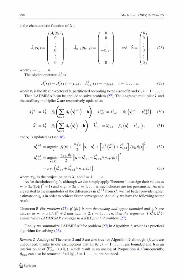
298 Mach Learn (2015) 99:287–325

is the characteristic function of Xi ,

Ai (xi ) =

⎛

⎜⎜⎜⎜⎜⎜⎜⎜⎝

Ai (xi )

0...

xi...

0

⎞

⎟⎟⎟⎟⎟⎟⎟⎟⎠

, An+i (xn+i ) =

⎛

⎜⎜⎜⎜⎜⎜⎜⎜⎝

00...

−xn+i...

0

⎞

⎟⎟⎟⎟⎟⎟⎟⎟⎠

, and b =

⎛

⎜⎜⎜⎜⎜⎜⎜⎜⎝

b0...

0...

0

⎞

⎟⎟⎟⎟⎟⎟⎟⎟⎠

, (28)

where i = 1, . . . , n.The adjoint operator A†

i is

A†i (y) = A†

i (y1) + yi+1, A†n+i (y) = −yi+1, i = 1, . . . , n, (29)

where yi is the i th sub-vector of y, partitioned according to the sizes of b and xi , i = 1, . . . , n.Then LADMPSAP can be applied to solve problem (27). The Lagrange multiplier λ and

the auxiliary multiplier λ are respectively updated as

λk+11 = λk

1 + βk

(n∑

i=1

Ai

(xk+1

i

)− b

), λk+1

i+1 = λki+1 + βk

(xk+1

i − xk+1n+i

), (30)

λk1 = λk

1 + βk

(n∑

i=1

Ai

(xk

i

)− b

), λ

ki+1 = λk

i+1 + βk

(xk

i − xkn+i

), (31)

and xi is updated as (see 16)

xk+1i = argmin

xfi (x) + ηiβk

2

∥∥∥x − xki +

[A†

i

(λ

k1

)+ λ

ki+1

]/(ηiβk)

∥∥∥2, (32)

xk+1n+i = argmin

x∈Xi

ηn+iβk

2

∥∥∥x − xkn+i − λ

ki+1/(ηn+iβk)

∥∥∥2

= πXi

(xk

n+i + λki+1/(ηn+iβk)

), (33)

where πXi is the projection onto Xi and i = 1, . . . , n.As for the choice of ηi ’s, although we can simply apply Theorem 1 to assign their values as

ηi > 2n(‖Ai‖2 + 1) and ηn+i > 2n, i = 1, . . . , n, such choices are too pessimistic. As ηi ’sare related to the magnitudes of the differences in xk+1

i from xki , we had better provide tighter

estimate on ηi ’s in order to achieve faster convergence. Actually, we have the following betterresult.

Theorem 5 For problem (27), if {βk} is non-decreasing and upper bounded and ηi ’s arechosen as ηi > n‖Ai‖2 + 2 and ηn+i > 2, i = 1, . . . , n, then the sequence {({xk

i },λk)}generated by LADMPSAP converge to a KKT point of problem (27).

Finally, we summarize LADMPSAP for problem (27) in Algorithm 2, which is a practicalalgorithm for solving (26).

Remark 2 Analogs of Theorems 2 and 3 are also true for Algorithm 2 although ∂ fn+i ’s areunbounded, thanks to our assumptions that all ∂ fi , i = 1, . . . , n, are bounded and b is aninterior point of

∑ni=1 Ai (Xi ), which result in an analog of Proposition 4. Consequently,

βmax can also be removed if all ∂ fi , i = 1, . . . , n, are bounded.

123

Mach Learn (2015) 99:287–325 299

Algorithm 2 LADMPSAP for (27), also a Practical Algorithm for (26).

Initialize: Set ρ0 > 1, ε1 > 0, ε2 > 0, βmax � 1 � β0 > 0, λ0 = ((λ01)T , . . . , (λ0

n+1)T )T , ηi >

n‖Ai ‖2 + 2, ηn+i > 2, x0i , x0

n+i = x0i , i = 1, . . . , n.

while (21) or (22) is not satisfied do

Step 1: Compute λk

as (31).Step 2: Update xi , i = 1, . . . , 2n, in parallel as (32)-(33).Step 3: Update λ by (30) and β by (18) and (20).

end while(Note that in (20), (21), and (22), n and Ai should be replaced by 2n and Ai , respectively.)

Remark 3 Since Algorithm 2 is an application of Algorithm 1 to problem (27), onlywith refined parameter estimation, its convergence rate in an ergodic sense is also

O(

1/∑K

k=0 β−1k

), where K is the number of iterations.

5 Proximal LADMPSAP for even more general convex programs

In LADMPSAP we have assumed that the subproblems (16) are easily solvable. In manymachine learning problems, the functions fi ’s are often matrix or vector norms or character-istic functions of convex sets. So this assumption often holds. Nonetheless, this assumptionis not always true, e.g., when fi is the logistic loss function [see (6)]. So in this section weaim at generalizing LADMPSAP to solve even more general convex programs (1).

We are interested in the case that fi can be decomposed into two components:

fi (xi ) = gi (xi ) + hi (xi ), (34)

where both gi and hi are convex, gi is C1,1:

‖∇gi (x) − ∇gi (y)‖ ≤ Li ‖x − y‖ , ∀x, y ∈ Rdi , (35)

and hi may not be differentiable but its proximal operation is easily solvable. For brevity, wecall Li the Lipschitz constant of ∇gi .

Recall that in each iteration of LADMPSAP, we have to solve subproblem (16). Sincenow we do not assume that the proximal operation of fi (7) is easily solvable, we may havedifficulty in solving subproblem (16). By (34), we write down (16) as

xk+1i = argmin

xi

hi (xi ) + gi (xi ) + σ(k)i

2

∥∥∥xi − xki + A†

i

(λ

k)

/σ(k)i

∥∥∥2, i = 1, . . . , n,

(36)

Since gi (xi ) + σ(k)i2

∥∥∥xi − xki + A†

i (λk)/σ

(k)i

∥∥∥2

is C1,1, we may also linearize it at xki and

add a proximal term. Such an idea leads to the following updating scheme of xi :

xk+1i = argmin

xi

hi (xi ) + gi

(xk

i

)+ σ

(k)i

2

∥∥∥A†i

(λ

k)

/σ(k)i

∥∥∥2

+⟨∇gi

(xk

i

)+ A†

i

(λ

k)

, xi − xki

⟩+ τ

(k)i

2

∥∥∥xi − xki

∥∥∥2

= argminxi

hi (xi ) + τ(k)i

2

∥∥∥∥∥xi − xki + 1

τ(k)i

[A†

i

(λ

k)

+ ∇gi

(xk

i

)]∥∥∥∥∥

2

, (37)

123

300 Mach Learn (2015) 99:287–325

Algorithm 3 Proximal LADMPSAP for Solving (1) with fi Satisfying (34).

Initialize: Set ρ0 > 1, β0 > 0, λ0, Ti ≥ Li , ηi > n‖Ai ‖2, x0i , i = 1, . . . , n.

while (39) or (40) is not satisfied do

Step 1: Compute λk

as (19).Step 2: Update xi ’s in parallel by solving

xk+1i = argmin

xihi (xi ) + τ

(k)i2

∥∥∥∥∥xi − xki + 1

τ(k)i

[A†

i (λk) + ∇gi

(xk

i

)]∥∥∥∥∥

2

, i = 1, . . . , n, (41)

where τ(k)i = Ti + βkηi .

Step 3: Update λ by (17) and β by (18) with ρ defined in (38).end while

where i = 1, . . . , n. The choice of τ(k)i is presented in Theorem 6, i.e. τ

(k)i = Ti + βkηi ,

where Ti ≥ Li and ηi > n‖Ai‖2 are both positive constants.By our assumption on hi , the above subproblems are easily solvable. The update of

Lagrange multiplier λ and β are still respectively goes as (17) and (18) but with

ρ =

⎧⎪⎪⎨

⎪⎪⎩

ρ0, if max({

‖Ai‖−1∥∥∥∇gi

(xk+1

i

)− ∇gi

(xk

i

)− τ(k)i

(xk+1

i − xki

)∥∥∥ ,

i = 1, . . . , n})

/‖b‖ < ε2,

1, otherwise.

(38)

The iteration terminates when the following two conditions are met:∥∥∥∥∥

n∑

i=1

Ai (xk+1i ) − b

∥∥∥∥∥ /‖b‖ < ε1, (39)

max({

‖Ai‖−1∥∥∥∇gi (x

k+1i ) − ∇gi (xk

i ) − τ(k)i (xk+1

i − xki )

∥∥∥ ,

i = 1, . . . , n})

/‖b‖ < ε2. (40)

These two conditions are also deduced from the KKT conditions.We call the above algorithm as proximal LADMPSAP and summarize it in Algorithm 3.As for the convergence of proximal LADMPSAP, we have the following theorem.

Theorem 6 (Convergence of proximal LADMPSAP) If βk is non-decreasing and upperbounded, τ

(k)i = Ti + βkηi , where Ti ≥ Li and ηi > n‖Ai‖2 are both positive constants,

i = 1, . . . , n, then {({xki },λk)} generated by proximal LADMPSAP converge to a KKT point

of problem (1).

We further have the following convergence rate theorem for proximal LADMPSAP in anergodic sense.

Theorem 7 (Convergence rate of proximal LADMPSAP) Define xKi = ∑K

k=0 γkxk+1i ,

where γk = β−1k /

∑Kj=0 β−1

j . Then the following inequality holds for xKi :

n∑

i=1

(fi

(xK

i

)− fi

(x∗

i

)+⟨A†

i (λ∗), xK

i − x∗i

⟩)+ αβ0

2

∥∥∥∥∥

n∑

i=1

Ai

(xK

i

)− b

∥∥∥∥∥

2

≤ C0/

K∑

k=0

2β−1k , (42)

123

Mach Learn (2015) 99:287–325 301

where

α−1 = (n + 1) max

(1,

{‖Ai‖2

ηi − n‖Ai‖2 , i = 1, . . . , n

})

and

C0 =n∑

i=1

β−10 τ

(0)i ‖x0

i − x∗i ‖2 + β−2

0 ‖λ0 − λ∗‖2.

When there are extra convex set constraints, xi ∈ Xi , i = 1, . . . , n, we can also introduceauxiliary variables as in Sect. 4 and have an analogy of Theorems 5 and 4.

Theorem 8 For problem (27), where fi is described at the beginning of Section 5, if βk

is non-decreasing and upper bounded and τ(k)i = Ti + ηiβk , where Ti ≥ Li , Tn+i =

0, ηi > n‖Ai‖2 + 2, and ηn+i > 2, i = 1, . . . , n, then {({xki },λk)} generated by proximal

LADMPSAP converge to a KKT point of problem (27). The convergence rate in an ergodic

sense is also O(

1/∑K

k=0 β−1k

), where K is the number of iterations.

6 Numerical results

In this section, we test the performance of LADMPSAP on three specific examples of problem(1), i.e., Latent low-rank representation [see (2)], nonnegative matrix completion [see (3)],and group sparse logistic regression with overlap [see (6)].

6.1 Solving latent low-rank representation

We first solve the latent LRR problem (Liu and Yan 2011) (2). In order to test LADMPSAPand related algorithms with data whose characteristics are controllable, we follow (Liu et al.2010) to generate synthetic data, which are parameterized as (s, p, d, r ), where s, p, d , and rare the number of independent subspaces, points in each subspace, and ambient and intrinsicdimensions, respectively. The number of scale variables and constraints is (sp) × d .

As first order methods are popular for solving convex programs in machine learning (Boydet al. 2011), here we compare LADMPSAP with several conceivable first order algorithms,including APG (Beck and Teboulle 2009), naive ADM, naive LADM, LADMGB, andLADMPS. Naive ADM and naive LADM are generalizations of ADM and LADM, respec-tively, which are straightforwardly generalized from two variables to multiple variables, asdiscussed in Sect. 3.1. Naive ADM is applied to solve (2) after rewriting the constraint of (2)as X = XP + QX + E, P = Z, Q = L. For LADMPS, βk is fixed in order to show the effec-tiveness of adaptive penalty. The parameters of APG and ADM are the same as those in (Linet al. 2009b) and (Liu and Yan 2011), respectively. For LADM, we follow the suggestions in(Yang and Yuan 2013) to fix its penalty parameter β at 2.5/ min(d, sp), where d × sp is thesize of X. For LADMGB, as there is no suggestion in He and Yuan (2013) on how to choosea fixed β, we simply set it the same as that in LADM. The rest of the parameters are the sameas those suggested in He et al. (2012). We fix β = σmax(X) min(d, sp)ε2 in LADMPS andset β0 = σmax(X) min(d, sp)ε2 and ρ0 = 10 in LADMPSAP. For LADMPSAP, we also setηZ = ηL = 1.02 × 3σ 2

max(X), where ηZ and ηL are the parameters ηi ’s in Algorithm 1 forZ and L, respectively. For the stopping criteria, ‖XZk + LkX + Ek − X‖/‖X‖ ≤ ε1 andmax(‖Zk − Zk−1‖, ‖Lk − Lk−1‖, ‖Ek − Ek−1‖)/‖X‖ ≤ ε2, with ε1 = 10−3 and ε2 = 10−4

123

302 Mach Learn (2015) 99:287–325

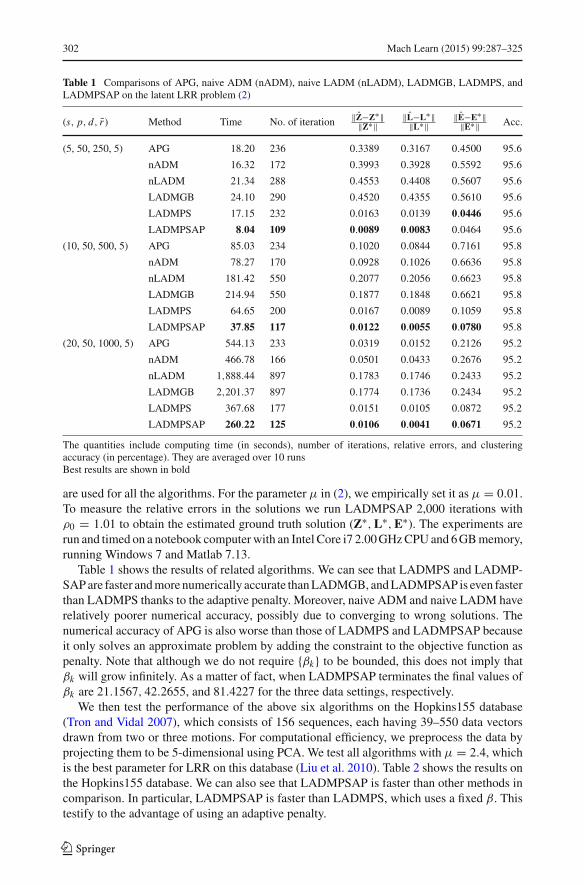
Table 1 Comparisons of APG, naive ADM (nADM), naive LADM (nLADM), LADMGB, LADMPS, andLADMPSAP on the latent LRR problem (2)

(s, p, d, r ) Method Time No. of iteration ‖Z−Z∗‖‖Z∗‖

‖L−L∗‖‖L∗‖

‖E−E∗‖‖E∗‖ Acc.

(5, 50, 250, 5) APG 18.20 236 0.3389 0.3167 0.4500 95.6

nADM 16.32 172 0.3993 0.3928 0.5592 95.6

nLADM 21.34 288 0.4553 0.4408 0.5607 95.6

LADMGB 24.10 290 0.4520 0.4355 0.5610 95.6

LADMPS 17.15 232 0.0163 0.0139 0.0446 95.6

LADMPSAP 8.04 109 0.0089 0.0083 0.0464 95.6

(10, 50, 500, 5) APG 85.03 234 0.1020 0.0844 0.7161 95.8

nADM 78.27 170 0.0928 0.1026 0.6636 95.8

nLADM 181.42 550 0.2077 0.2056 0.6623 95.8

LADMGB 214.94 550 0.1877 0.1848 0.6621 95.8

LADMPS 64.65 200 0.0167 0.0089 0.1059 95.8

LADMPSAP 37.85 117 0.0122 0.0055 0.0780 95.8

(20, 50, 1000, 5) APG 544.13 233 0.0319 0.0152 0.2126 95.2

nADM 466.78 166 0.0501 0.0433 0.2676 95.2

nLADM 1,888.44 897 0.1783 0.1746 0.2433 95.2

LADMGB 2,201.37 897 0.1774 0.1736 0.2434 95.2

LADMPS 367.68 177 0.0151 0.0105 0.0872 95.2

LADMPSAP 260.22 125 0.0106 0.0041 0.0671 95.2

The quantities include computing time (in seconds), number of iterations, relative errors, and clusteringaccuracy (in percentage). They are averaged over 10 runsBest results are shown in bold

are used for all the algorithms. For the parameter μ in (2), we empirically set it as μ = 0.01.To measure the relative errors in the solutions we run LADMPSAP 2,000 iterations withρ0 = 1.01 to obtain the estimated ground truth solution (Z∗, L∗, E∗). The experiments arerun and timed on a notebook computer with an Intel Core i7 2.00 GHz CPU and 6 GB memory,running Windows 7 and Matlab 7.13.

Table 1 shows the results of related algorithms. We can see that LADMPS and LADMP-SAP are faster and more numerically accurate than LADMGB, and LADMPSAP is even fasterthan LADMPS thanks to the adaptive penalty. Moreover, naive ADM and naive LADM haverelatively poorer numerical accuracy, possibly due to converging to wrong solutions. Thenumerical accuracy of APG is also worse than those of LADMPS and LADMPSAP becauseit only solves an approximate problem by adding the constraint to the objective function aspenalty. Note that although we do not require {βk} to be bounded, this does not imply thatβk will grow infinitely. As a matter of fact, when LADMPSAP terminates the final values ofβk are 21.1567, 42.2655, and 81.4227 for the three data settings, respectively.

We then test the performance of the above six algorithms on the Hopkins155 database(Tron and Vidal 2007), which consists of 156 sequences, each having 39–550 data vectorsdrawn from two or three motions. For computational efficiency, we preprocess the data byprojecting them to be 5-dimensional using PCA. We test all algorithms with μ = 2.4, whichis the best parameter for LRR on this database (Liu et al. 2010). Table 2 shows the results onthe Hopkins155 database. We can also see that LADMPSAP is faster than other methods incomparison. In particular, LADMPSAP is faster than LADMPS, which uses a fixed β. Thistestify to the advantage of using an adaptive penalty.

123

Mach Learn (2015) 99:287–325 303

Table 2 Comparisons of APG, naive ADM (nADM), naive LADM (nLADM), LADMGB, LADMPS, andLADMPSAP on the Hopkins155 database

Method Time (s) No. of iteration Error (%)

APG 10.37 67 8.33

nADM 24.76 144 8.33

nLADM 15.50 112 8.33

LADMGB 16.05 113 8.36

LADMPS 15.58 113 8.33

LADMPSAP 3.80 26 8.33

The quantities include average computing time, average number of iterations, and average classification errorson all 156 sequencesBest results are shown in bold

Table 3 Comparisons on the NMC problem (3) with synthetic data, averaged on 10 runs

X LADM LADMPSAP

n q (%) t/dr No. ofiteration

Time (s) RelErr FA No. ofiteration

Time (s) RelErr FA

1,000 20 10.05 375 177.92 1.35E−5 6.21E−4 58 24.94 9.67E−6 0

10 5.03 1,000 459.70 4.60E−5 6.50E−4 109 42.68 1.72E−5 0

5,000 20 50.05 229 1,613.68 1.08E−5 1.93E−4 49 369.96 9.05E−6 0

10 25.03 539 2,028.14 1.20E−5 7.70E−5 89 365.26 9.76E−6 0

10,000 10 50.03 463 6,679.59 1.11E−5 4.18E−5 89 1584.39 1.03E−5 0

q, t , and dr denote, respectively, the sample ratio, the number of measurements t = q(mn), and the “degreeof freedom” defined by dr = r(m + n − r) for an m × n matrix with rank r and q. Here we set m = n andfix r = 10 in all the testsBest results are shown in bold

6.2 Solving nonnegative matrix completion

This subsection evaluates the performance of the practical LADMPSAP proposed in Sect. 4for solving nonnegative matrix completion (Xu et al. 2011) (3).

We first evaluate the numerical performance on synthetic data to demonstrate the superi-ority of practical LADMPSAP over the conventional LADM9 (Yang and Yuan 2013). Thenonnegative low-rank matrix X0 is generated by truncating the singular values of a randomlygenerated matrix. As LADM cannot handle the nonnegativity constraint, it actually solvethe standard matrix completion problem, i.e., (3) without the nonnegativity constraint. ForLADMPSAP, we follow the conditions in Theorem 5 to set ηi ’s and set the rest of the para-meters the same as those in Sect. 6.1. The stopping tolerances are set as ε1 = ε2 = 10−5.The numerical comparison is shown in Table 3, where the relative nonnegative feasibility(FA) is defined as (Xu et al. 2011):

FA: = ‖ min(X, 0)‖/‖X0‖,in which X0 is the ground truth and X is the computed solution. It can be seen that thenumerical performance of LADMPSAP is much better than that of LADM, thus again verifies

9 Code available at http://math.nju.edu.cn/~jfyang/IADM_NNLS/index.html.

123

304 Mach Learn (2015) 99:287–325

(a) Original (b) Corrupted (c) FPCA (d) LADM (e) LADMPSAP

Fig. 1 Image inpainting by FPCA, LADM and LADMPSAP

Table 4 Comparisons on the image inpainting problem. “PSNR” stands for “Peak Signal to Noise Ratio”measured in decibel (dB)

Method No. of iteration Time (s) PSNR (dB) FA

FPCA 179 228.99 27.77 9.41E−4

LADM 228 207.95 26.98 2.92E−3

LADMPSAP 143 134.89 31.39 0

Best results are shown in bold

the efficiency of our proposed parallel splitting and adaptive penalty scheme for enhancingADM/LADM type algorithms.

We then consider the image inpainting problem, which is to fill in the missing pixel valuesof a corrupted image. As the pixel values are nonnegative, the image inpainting problemcan be formulated as the NMC problem. To prepare a low-rank image, we also truncate thesingular values of a 1,024 × 1,024 grayscale image “man”10 to obtain an image of rank 40,shown in Fig. 1a, b. The corrupted image is generated from the original image (all pixels havebeen normalized in the range of [0, 1]) by sampling 20 % of the pixels uniformly at randomand adding Gaussian noise with mean zero and standard deviation 0.1.

Besides LADM, here we also consider another recently proposed fixed point continuationwith approximate SVD [FPCA (Ma et al. 2011)] on this problem. Similar to LADM, the codeof FPCA11 can only solve the standard matrix completion problem without the nonnegativityconstraint. This time we set ε1 = 10−3 and ε2 = 10−1 as the thresholds for stopping criteria.The recovered images are shown in Fig. 1c–e and the quantitative results are in Table 4. Onecan see that on our test image both the qualitative and the quantitative results of LADMPSAPare better than those of FPCA and LADM. Note that LADMPSAP is faster than FPCA andLADM even though they do not handle the nonnegativity constraint.

6.3 Solving group sparse logistic regression with overlap

In this subsection, we apply proximal LADMPSAP to solve the problem of group sparselogistic regression with overlap (5).

The Lipschitz constant of the gradient of logistic function with respect to w can be provento be Lw ≤ 1

4s ‖X‖22, where X = (x1, x2, . . . , xs). Thus (5) can be directly solved by

Algorithm 3.

10 Available at http://sipi.usc.edu/database/.11 Code available at http://www1.se.cuhk.edu.hk/~sqma/softwares.html.

123

Mach Learn (2015) 99:287–325 305

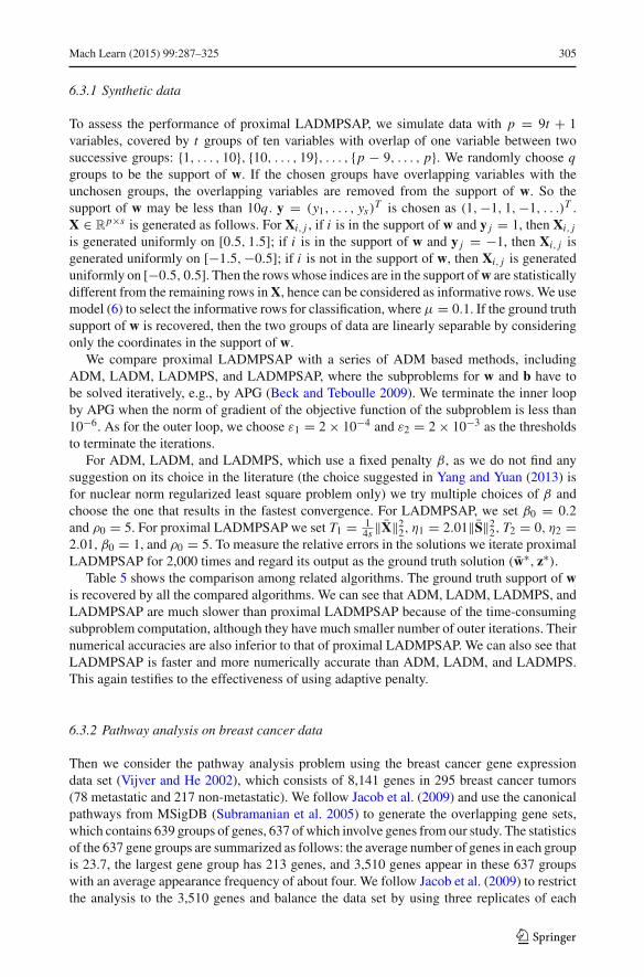
6.3.1 Synthetic data

To assess the performance of proximal LADMPSAP, we simulate data with p = 9t + 1variables, covered by t groups of ten variables with overlap of one variable between twosuccessive groups: {1, . . . , 10}, {10, . . . , 19}, . . . , {p − 9, . . . , p}. We randomly choose qgroups to be the support of w. If the chosen groups have overlapping variables with theunchosen groups, the overlapping variables are removed from the support of w. So thesupport of w may be less than 10q . y = (y1, . . . , ys)

T is chosen as (1,−1, 1,−1, . . .)T .X ∈ R

p×s is generated as follows. For Xi, j , if i is in the support of w and y j = 1, then Xi, j

is generated uniformly on [0.5, 1.5]; if i is in the support of w and y j = −1, then Xi, j isgenerated uniformly on [−1.5,−0.5]; if i is not in the support of w, then Xi, j is generateduniformly on [−0.5, 0.5]. Then the rows whose indices are in the support of w are statisticallydifferent from the remaining rows in X, hence can be considered as informative rows. We usemodel (6) to select the informative rows for classification, where μ = 0.1. If the ground truthsupport of w is recovered, then the two groups of data are linearly separable by consideringonly the coordinates in the support of w.

We compare proximal LADMPSAP with a series of ADM based methods, includingADM, LADM, LADMPS, and LADMPSAP, where the subproblems for w and b have tobe solved iteratively, e.g., by APG (Beck and Teboulle 2009). We terminate the inner loopby APG when the norm of gradient of the objective function of the subproblem is less than10−6. As for the outer loop, we choose ε1 = 2 × 10−4 and ε2 = 2 × 10−3 as the thresholdsto terminate the iterations.

For ADM, LADM, and LADMPS, which use a fixed penalty β, as we do not find anysuggestion on its choice in the literature (the choice suggested in Yang and Yuan (2013) isfor nuclear norm regularized least square problem only) we try multiple choices of β andchoose the one that results in the fastest convergence. For LADMPSAP, we set β0 = 0.2and ρ0 = 5. For proximal LADMPSAP we set T1 = 1

4s ‖X‖22, η1 = 2.01‖S‖2

2, T2 = 0, η2 =2.01, β0 = 1, and ρ0 = 5. To measure the relative errors in the solutions we iterate proximalLADMPSAP for 2,000 times and regard its output as the ground truth solution (w∗, z∗).

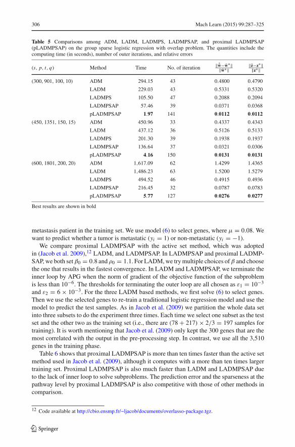
Table 5 shows the comparison among related algorithms. The ground truth support of wis recovered by all the compared algorithms. We can see that ADM, LADM, LADMPS, andLADMPSAP are much slower than proximal LADMPSAP because of the time-consumingsubproblem computation, although they have much smaller number of outer iterations. Theirnumerical accuracies are also inferior to that of proximal LADMPSAP. We can also see thatLADMPSAP is faster and more numerically accurate than ADM, LADM, and LADMPS.This again testifies to the effectiveness of using adaptive penalty.

6.3.2 Pathway analysis on breast cancer data

Then we consider the pathway analysis problem using the breast cancer gene expressiondata set (Vijver and He 2002), which consists of 8,141 genes in 295 breast cancer tumors(78 metastatic and 217 non-metastatic). We follow Jacob et al. (2009) and use the canonicalpathways from MSigDB (Subramanian et al. 2005) to generate the overlapping gene sets,which contains 639 groups of genes, 637 of which involve genes from our study. The statisticsof the 637 gene groups are summarized as follows: the average number of genes in each groupis 23.7, the largest gene group has 213 genes, and 3,510 genes appear in these 637 groupswith an average appearance frequency of about four. We follow Jacob et al. (2009) to restrictthe analysis to the 3,510 genes and balance the data set by using three replicates of each

123

306 Mach Learn (2015) 99:287–325

Table 5 Comparisons among ADM, LADM, LADMPS, LADMPSAP, and proximal LADMPSAP(pLADMPSAP) on the group sparse logistic regression with overlap problem. The quantities include thecomputing time (in seconds), number of outer iterations, and relative errors

(s, p, t, q) Method Time No. of iteration ‖ ˆw−w∗‖‖w∗‖

‖z−z∗‖‖z∗‖

(300, 901, 100, 10) ADM 294.15 43 0.4800 0.4790

LADM 229.03 43 0.5331 0.5320

LADMPS 105.50 47 0.2088 0.2094

LADMPSAP 57.46 39 0.0371 0.0368

pLADMPSAP 1.97 141 0.0112 0.0112

(450, 1351, 150, 15) ADM 450.96 33 0.4337 0.4343

LADM 437.12 36 0.5126 0.5133

LADMPS 201.30 39 0.1938 0.1937

LADMPSAP 136.64 37 0.0321 0.0306

pLADMPSAP 4.16 150 0.0131 0.0131

(600, 1801, 200, 20) ADM 1,617.09 62 1.4299 1.4365

LADM 1,486.23 63 1.5200 1.5279

LADMPS 494.52 46 0.4915 0.4936

LADMPSAP 216.45 32 0.0787 0.0783

pLADMPSAP 5.77 127 0.0276 0.0277

Best results are shown in bold

metastasis patient in the training set. We use model (6) to select genes, where μ = 0.08. Wewant to predict whether a tumor is metastatic (yi = 1) or non-metastatic (yi = −1).

We compare proximal LADMPSAP with the active set method, which was adoptedin (Jacob et al. 2009),12 LADM, and LADMPSAP. In LADMPSAP and proximal LADMP-SAP, we both set β0 = 0.8 and ρ0 = 1.1. For LADM, we try multiple choices of β and choosethe one that results in the fastest convergence. In LADM and LADMPSAP, we terminate theinner loop by APG when the norm of gradient of the objective function of the subproblemis less than 10−6. The thresholds for terminating the outer loop are all chosen as ε1 = 10−3

and ε2 = 6 × 10−3. For the three LADM based methods, we first solve (6) to select genes.Then we use the selected genes to re-train a traditional logistic regression model and use themodel to predict the test samples. As in Jacob et al. (2009) we partition the whole data setinto three subsets to do the experiment three times. Each time we select one subset as the testset and the other two as the training set (i.e., there are (78 + 217) × 2/3 = 197 samples fortraining). It is worth mentioning that Jacob et al. (2009) only kept the 300 genes that are themost correlated with the output in the pre-processing step. In contrast, we use all the 3,510genes in the training phase.

Table 6 shows that proximal LADMPSAP is more than ten times faster than the active setmethod used in Jacob et al. (2009), although it computes with a more than ten times largertraining set. Proximal LADMPSAP is also much faster than LADM and LADMPSAP dueto the lack of inner loop to solve subproblems. The prediction error and the sparseness at thepathway level by proximal LADMPSAP is also competitive with those of other methods incomparison.

12 Code available at http://cbio.ensmp.fr/~ljacob/documents/overlasso-package.tgz.

123

Mach Learn (2015) 99:287–325 307

Table 6 Comparisons among the Active Set method (Jacob et al. 2009), LADM, LADMPSAP, and proximalLADMPSAP (pLADMPSAP) on the pathway analysis

Method Time Error No. of pathway

Active set 2,179 0.36±0.03 6, 5, 78

LADM 2,433 0.315±0.049 7, 9, 10

LADMPSAP 1,593 0.329±0.011 7, 9, 9

pLADMPSAP 179 0.312±0.026 4, 6, 6

We present the CPU time (in seconds), classification error rate, and number of pathways. Results are estimatedby three-fold cross validation. No. of Pathway gives the number of pathways that the selected genes belongto in each of the cross validationBest results are shown in bold

7 Conclusions

In this paper, we propose linearized alternating direction method with parallel splitting andadaptive penalty (LADMPSAP) for efficiently solving linearly constrained multi-block sep-arable convex programs, which are abundant in machine learning. LADMPSAP fully utilizesthe properties that the proximal operations of the component objective functions and the pro-jections onto convex sets are easily solvable, which are usually satisfied by machine learningproblems, making each of its iterations cheap. It is also highly parallel, making it appealingfor parallel or distributed computing. Numerical experiments testify to the advantages ofLADMPSAP over other possible first order methods.

Although LADMPSAP is inherently parallel, when solving the proximal operations ofcomponent objective functions we will still face basic numerical algebraic computations.So for particular large scale machine learning problems, it will be interesting to integratethe existing distributed computing techniques [e.g., parallel incomplete Cholesky factoriza-tion (Chang et al. 2007; Chang 2011) and caching factorization techniques (Boyd et al. 2011)]with our LADMPSAP in order to effectively address the scalability issues.

Acknowledgments Z. Lin is supported by 973 Program of China (No. 2015CB3525), NSFC (Nos. 61272341and 61231002), and Microsoft Research Asia Collaborative Research Program. R. Liu is supported by NSFC(No. 61300086), the China Postdoctoral Science Foundation (Nos. 2013M530917 and 2014T70249), theFundamental Research Funds for the Central Universities (No. DUT12RC(3)67) and the Open Project Programof the State Key Lab of CAD&CG (No. A1404), Zhejiang University. Z. Lin also thanks Xiaoming Yuan,Wotao Yin, and Edward Chang for valuable discussions and HTC for financial support.

Appendix 1: Proof of Theorem 1

To prove this theorem, we first have the following lemmas and propositions.

Lemma 1 (KKT Condition) The Kuhn–Karush–Tucker (KKT) condition of problem (1) isthat there exists (x∗

1, . . . , x∗n,λ∗), such that

n∑

i=1

Ai(x∗

i

) = b, (43)

−A†i (λ

∗) ∈ ∂ fi(x∗

i

), i = 1, . . . , n, (44)

where ∂ fi is the subgradient of fi .

123

308 Mach Learn (2015) 99:287–325

The first is the feasibility condition and the second is the duality condition. Such(x∗

1, . . . , x∗n,λ∗) is called a KKT point of problem (1).

Lemma 2 For {(xk1, . . . , xk

n, λk)} generated by Algorithm 1, we have that

− σ(k)i

(xk+1

i − uki

)∈ ∂ fi

(xk+1

i

), i = 1, . . . , n, (45)

where uki = xk

i − A†i (λ

k)/σ

(k)i .

This can be easily proved by checking the optimality conditions of (16).

Lemma 3 For {(xk1, . . . , xk

n, λk)} generated by Algorithm 1 and a KKT point (x∗1, . . . , x∗

n,λ∗)of problem (1), the following inequality holds:

⟨−σ

(k)i

(xk+1

i − uki

)+ A†

i (λ∗), xk+1

i − x∗i

⟩≥ 0, i = 1, . . . , n. (46)

This can be deduced by the monotonicity of subgradient mapping (Rockafellar 1970).

Lemma 4 For {(xk1, . . . , xk

n, λk)} generated by Algorithm 1 and a KKT point (x∗1, . . . , x∗

n,λ∗)of problem (1), we have that

βk

n∑

i=1

σ(k)i

∥∥∥xk+1i − x∗

i

∥∥∥2 +

∥∥∥λk+1 − λ∗∥∥∥

2(47)

= βk

n∑

i=1

σ(k)i

∥∥∥xki − x∗

i

∥∥∥2 +

∥∥∥λk − λ∗∥∥∥

2(48)

−2βk

n∑

i=1

⟨xk+1

i − x∗i ,−σ

(k)i

(xk+1

i − uki

)+ A†

i (λ∗)⟩

(49)

−βk

n∑

i=1

σ(k)i

∥∥∥xk+1i − xk

i

∥∥∥2 −

∥∥∥λk+1 − λk∥∥∥

2(50)

− 2βk

n∑

i=1

σ(k)i

⟨xk+1

i − x∗i , xk

i − uki

⟩(51)

+ 2⟨λk+1 − λk,λk+1

⟩. (52)

Proof This can be easily checked. First, we add (49) and (51) to have

−2βk

n∑

i=1

⟨xk+1

i − x∗i ,−σ

(k)i

(xk+1

i − uki

)+ A†

i (λ∗)⟩

(53)

− 2βk

n∑

i=1

σ(k)i

⟨xk+1

i − x∗i , xk

i − uki

⟩(54)

= −2βk

n∑

i=1

⟨xk+1

i − x∗i , A†

i (λ∗)⟩+ 2βk

n∑

i=1

σ(k)i

⟨xk+1

i − x∗i , xk+1

i − xki

⟩(55)

= − 2βk

n∑

i=1

⟨Ai

(xk+1

i − x∗i

),λ∗⟩+ 2βk

n∑

i=1

σ(k)i

⟨xk+1

i − x∗i , xk+1

i − xki

⟩(56)

123

Mach Learn (2015) 99:287–325 309

= −2

⟨βk

n∑

i=1

Ai

(xk+1

i − x∗i

),λ∗

⟩+ 2βk

n∑

i=1

σ(k)i

⟨xk+1

i − x∗i , xk+1

i − xki

⟩(57)

= −2

⟨βk

(n∑

i=1

Ai

(xk+1

i

)− b

),λ∗

⟩(58)

+ 2βk

n∑

i=1

σ(k)i

⟨xk+1

i − x∗i , xk+1

i − xki

⟩(59)

= −2⟨λk+1 − λk,λ∗⟩+ 2βk

n∑

i=1

σ(k)i

⟨xk+1

i − x∗i , xk+1

i − xki

⟩, (60)

where we have used (43) in (57). Then we apply the identity

2⟨ak+1 − a∗, ak+1 − ak

⟩ = ‖ak+1 − a∗‖2 − ‖ak − a∗‖2 + ‖ak+1 − ak‖2 (61)

to see that (47)–(52) holds. ��Proposition 2 For {(xk

1, . . . , xkn, λk)}generated by Algorithm 1 and a KKT point (x∗

1, . . . , x∗n,

λ∗) of problem (1), the following inequality holds:

βk

n∑

i=1

σ(k)i

∥∥∥xk+1i − x∗

i

∥∥∥2 +

∥∥∥λk+1 − λ∗∥∥∥

2(62)

≤ βk

n∑

i=1

σ(k)i

∥∥∥xki − x∗

i

∥∥∥2 +

∥∥∥λk − λ∗∥∥∥

2(63)

− 2βk

n∑

i=1

⟨xk+1

i − x∗i ,−σ

(k)i

(xk+1

i − uki

)+ A†

i (λ∗)⟩

(64)

−βk

n∑

i=1

(σ

(k)i − nβk‖Ai‖2

) ∥∥∥xk+1i − xk

i

∥∥∥2 −

∥∥∥λk − λk∥∥∥

2. (65)

Proof We continue from (51)–(52). As σ(k)i (xk

i − uki ) = A†

i (λk), we have

−2βk

n∑

i=1

σ(k)i

⟨xk+1

i − x∗i , xk

i − uki

⟩+ 2

⟨λk+1 − λk,λk+1

⟩(66)

= −2βk

n∑

i=1

⟨Ai

(xk+1

i − x∗i

), λ

k⟩+ 2

⟨λk+1 − λk,λk+1

⟩(67)

= −2βk

⟨n∑

i=1

Ai

(xk+1

i

)−

n∑

i=1

Ai(x∗

i

), λ

k⟩

+ 2⟨λk+1 − λk,λk+1

⟩(68)

= −2⟨λk+1 − λk, λ

k⟩+ 2

⟨λk+1 − λk,λk+1

⟩(69)

= 2⟨λk+1 − λk,λk+1 − λ

k⟩

(70)

= ‖λk+1 − λk‖2 + ‖λk+1 − λk‖2 − ‖λk − λ

k‖2 (71)

= ‖λk+1 − λk‖2 + β2k

∥∥∥∥∥

n∑

i=1

Ai

(xk+1

i − xki

)∥∥∥∥∥

2

− ‖λk − λk‖2 (72)

123

310 Mach Learn (2015) 99:287–325

≤ ‖λk+1 − λk‖2 + β2k

(n∑

i=1

‖Ai‖∥∥∥xk+1

i − xki

∥∥∥

)2

− ‖λk − λk‖2 (73)

≤ ‖λk+1 − λk‖2 + nβ2k

n∑

i=1

‖Ai‖2∥∥∥xk+1

i − xki

∥∥∥2 − ‖λk − λ

k‖2 (74)

Plugging the above into (51)–(52), we have (62)–(65). ��Remark 4 Proposition 2 shows that the sequence {(xk

1, . . . , xkn, λk)} is Fejér monotone.

Proposition 2 is different from Lemma 1 in Supplementary Material of Lin et al. (2011)because for n > 2 we cannot obtain an (in)equality that is similar to Lemma 1 in Supple-mentary Material of Lin et al. (2011) such that each term with minus sign could be madenon-positive. Such Fejér monotone (in)equalities are the corner stones for proving the con-vergence of Lagrange multiplier based optimization algorithms. As a result, we cannot provethe convergence of the naively generalized LADM for the multi-block case.

Then we have the following proposition.

Proposition 3 Let σ(k)i = ηiβk, i = 1, . . . , n. If {βk} is non-decreasing, ηi > n‖Ai‖2, i =

1, . . . , n, {(xk1, . . . , xk

n, λk)} is generated by Algorithm 1, and (x∗1, . . . , x∗

n,λ∗) is any KKTpoint of problem (1), then

(1){∑n

i=1 ηi‖xki − x∗

i ‖2 + β−2k ‖λk − λ∗‖2

}is nonnegative and non-increasing.

(2) ‖xk+1i − xk

i ‖ → 0, i = 1, . . . , n, and β−1k ‖λk − λ

k‖ → 0.

(3)∑+∞

k=1 β−1k

⟨xk+1

i − x∗i ,−σ

(k)i (xk+1

i − uki ) + A†

i (λ∗)⟩< +∞, i = 1, . . . , n.

Proof We divide both sides of (62)–(65) by β2k to have

n∑

i=1

ηi

∥∥∥xk+1i − x∗

i

∥∥∥2 + β−2

k

∥∥∥λk+1 − λ∗∥∥∥

2(75)

≤n∑

i=1

ηi‖xki − x∗

i ‖2 + β−2k ‖λk − λ∗‖2 (76)

− 2β−1k

n∑

i=1

⟨xk+1

i − x∗i ,−σ

(k)i

(xk+1

i − uki

)+ A†

i (λ∗)⟩

(77)

−n∑

i=1

(ηi − n‖Ai‖2)

∥∥∥xk+1i − xk

i

∥∥∥2

(78)

−β−2k ‖λk − λ

k‖2. (79)

Then by (46), ηi > n‖Ai‖2 and the non-decrement of {βk}, we can easily obtain (1). Second,we sum both sides of (75)–(79) over k to have

2+∞∑

k=0

β−1k

n∑

i=1

⟨xk+1

i − x∗,−σ(k)i

(xk+1

i − uki

)+ A†

i (λ∗)⟩

(80)

+n∑

i=1

(ηi − n‖Ai‖2)

+∞∑

k=0

∥∥∥xk+1i − xk

i

∥∥∥2

(81)

123

Mach Learn (2015) 99:287–325 311

++∞∑

k=0

β−2k ‖λk − λ

k‖2 (82)

≤n∑

i=1

ηi∥∥x0

i − x∗∥∥2 + β−20 ‖λ0 − λ∗‖2. (83)

Then (2) and (3) can be easily deduced. ��Now we are ready to prove Theorem 1. The proof resembles that in (Lin et al. 2011).

Proof of Theorem 1 By Proposition 3-(1) and the boundedness of {βk}, {(xk1, . . . , xk

n,λk)} is

bounded, hence has an accumulation point, say (xk j1 , . . . , x

k jn ,λk j ) → (x∞

1 , . . . , x∞n ,λ∞).

We accomplish the proof in two steps.1. We first prove that (x∞

1 , . . . , x∞n ,λ∞) is a KKT point of problem (1).

By Proposition 3-(2),n∑

i=1

Ai

(xk

i

)− b = β−1

k

(λ

k − λk)

→ 0.

So any accumulation point of {(xk1, . . . , xk

n)} is a feasible solution.

Since −σ(k j −1)

i (xk ji − u

k j −1i ) ∈ ∂ fi (x

k ji ), we have

n∑

i=1

fi

(x

k ji

)≤

n∑

i=1

fi(x∗

i

)+n∑

i=1

⟨x

k ji − x∗

i ,−σ(k j −1)

i

(x

k ji − u

k j −1i

)⟩

=n∑

i=1

fi(x∗

i

)+n∑

i=1

⟨x

k ji − x∗

i ,−ηiβk j −1

(x

k ji − x

k j −1i

)− A†

i

(λ

k j −1)⟩

.

Let j → +∞. By observing Proposition 3-(2) and the boundedness of {βk}, we haven∑

i=1

fi(x∞

i

) ≤n∑

i=1

fi(x∗

i

)+n∑

i=1

⟨x∞

i − x∗i ,−A†

i (λ∞)⟩

=n∑

i=1

fi(x∗

i

)−n∑

i=1

⟨A(x∞

i − x∗i

),λ∞⟩

=n∑

i=1

fi(x∗

i

)−⟨

n∑

i=1

A(x∞

i

)− b,λ∞⟩

=n∑

i=1

fi(x∗

i

).

So we conclude that (x∞1 , . . . , x∞

n ) is an optimal solution to (1).

Again by −σ(k j −1)

i (xk ji − u

k j −1i ) ∈ ∂ fi (x

k ji ) we have

fi (x) ≥ fi

(x

k ji

)+⟨x − x

k ji ,−σ

(k j −1)

i (xk ji − u

k j −1i )

⟩

= fi

(x

k ji

)+⟨x − x

k ji ,−ηiβk j −1

(x

k ji − x

k j −1i

)− A†

i

(λ

k j −1)⟩

.

Fixing x and letting j → +∞, we see that

fi (x) ≥ fi (x∞i ) +

⟨x − x∞

i ,−A†i (λ

∞)⟩, ∀x.

123

312 Mach Learn (2015) 99:287–325

So −A†i (λ

∞) ∈ ∂ fi (x∞i ), i = 1, . . . , n. Thus (x∞

1 , . . . , x∞n ,λ∞) is a KKT point of problem

(1).2. We next prove that the whole sequence {(xk

1, . . . , xkn,λk)} converges to (x∞

1 , . . . , x∞n ,

λ∞).By choosing (x∗

1, . . . , x∗n,λ∗) = (x∞

1 , . . . , x∞n ,λ∞) in Proposition 3, we have

n∑

i=1

ηi

∥∥∥xk ji − x∞

i

∥∥∥2 + β−2

k j

∥∥∥λk j − λ∞∥∥∥

2 → 0.

By Proposition 3-(1), we readily have

n∑

i=1

ηi

∥∥∥xki − x∞

i

∥∥∥2 + β−2

k

∥∥∥λk − λ∞∥∥∥

2 → 0.

So (xk1, . . . , xk

n,λk) → (x∞1 , . . . , x∞

n ,λ∞).As (x∞

1 , . . . , x∞n ,λ∞) can be an arbitrary accumulation point of {(xk

1, . . . , xkn,λk)}, we

conclude that {(xk1, . . . , xk

n,λk)} converge to a KKT point of problem (1). ��

Appendix 2: Proof of Theorem 2

We first have the following proposition.

Proposition 4 If {βk} is non-decreasing and unbounded, ηi > n‖Ai‖2 and ∂ fi (x) is boundedfor i = 1, . . . , n, then Proposition 3 holds and

β−1k λk → 0. (84)

Proof As the conditions here are stricter than those in Proposition 3, Proposition 3 holds.Then we have that {β−1

k ‖λk − λ∗‖} is bounded due to Proposition 3-(1). So {β−1k λk} is

bounded due to β−1k ‖λk‖ ≤ β−1

k ‖λk − λ∗‖ + β−1k ‖λ∗‖. {β−1

k λk} is also bounded thanks to

Proposition 3-(2).We rewrite Lemma 2 as

− ηi

(xk+1

i − xki

)− A†

i

(β−1

k λk)

∈ β−1k ∂ fi

(xk+1

i

), i = 1, . . . , n. (85)

Then by the boundedness of ∂ fi (x), the unboundedness of {βk} and Proposition 3-(2), lettingk → +∞, we have that

A†i (λ

∞) = 0, i = 1, . . . , n. (86)

where λ∞

is any accumulation point of {β−1k λ

k}, which is the same as that of {β−1k λk} due

to Proposition 3-(2).Recall that we have assumed that the mapping A(x1, . . . , xn) ≡ ∑n

i=1 Ai (xi ) is onto. So

∩ni=1null(A†

i ) = 0. Therefore by (86), λ∞ = 0. ��

Based on Proposition 4, we can prove Theorem 2 as follows.

Proof of Theorem 2 When {βk} is bounded, the convergence has been proven in Theorem 1.In the following, we only focus on the case that {βk} is unbounded.

By Proposition 3-(1), {(xk1, . . . , xk

n)} is bounded, hence has at least one accumulation point(x∞

1 , . . . , x∞n ). By Proposition 3-(2), (x∞

1 , . . . , x∞n ) is a feasible solution.

123

Mach Learn (2015) 99:287–325 313

Since∑+∞

k=1 β−1k = +∞ and Proposition 3-(3), there exists a subsequence {(xk j

1 , . . . , xk jn )}

such that⟨x

k ji − x∗

i ,−σ(k j −1)

i

(x

k ji − u

k j −1i

)+ A†

i (λ∗)⟩→ 0, i = 1, . . . , n. (87)

As pk ji ≡ −σ

(k j −1)

i (xk ji − u

k j −1i ) ∈ ∂ fi (x

k ji ) and ∂ fi is bounded, we may assume that

xk ji → x∞

i and pk ji → p∞

i .

It can be easily proven that

p∞i ∈ ∂ fi (x∞

i ).

Then letting j → ∞ in (87), we have⟨x∞

i − x∗i , p∞

i + A†i (λ

∗)⟩= 0, i = 1, . . . , n. (88)

Then by pk ji ∈ ∂ fi (x

k ji ),

n∑

i=1

fi

(x

k ji

)≤

n∑

i=1

fi(x∗

i

)+n∑

i=1

⟨x

k ji − x∗

i , pk ji

⟩. (89)

Letting j → ∞ and making use of (88), we have

n∑

i=1

fi(x∞

i

) ≤n∑

i=1

fi(x∗

i

)+n∑

i=1

⟨x∞

i − x∗i , p∞

i

⟩

=n∑

i=1

fi(x∗

i

)−n∑

i=1

⟨x∞

i − x∗i , A†

i (λ∗)⟩

=n∑

i=1

fi(x∗

i

)−n∑

i=1

⟨Ai(x∞

i − x∗i

),λ∗⟩

=n∑

i=1

fi(x∗

i

). (90)

So together with the feasibility of {(x∞1 , . . . , x∞

n )} we have that {(xk j1 , . . . , x

k jn )} converges

to an optimal solution {(x∞1 , . . . , x∞

n )} to (1).Finally, we set x∗

i = x∞i and λ∗ be the corresponding Lagrange multiplier λ∞ in Propo-

sition 3. By Proposition 4, we have that

n∑

i=1

ηi

∥∥∥xk ji − x∞

i

∥∥∥2 + β−2

k j

∥∥∥λk j − λ∞∥∥∥

2 → 0.

By Proposition 3-(1), we readily have

n∑

i=1

ηi‖xki − x∞

i ‖2 + β−2k ‖λk − λ∞‖2 → 0.

So (xk1, . . . , xk

n) → (x∞1 , . . . , x∞

n ). ��

123

314 Mach Learn (2015) 99:287–325

Appendix 3: Proof of Theorem 3

Proof of Theorem 3 We first prove that there exist linear mappings Bi , i = 1, . . . , n, suchthat Bi ’s are not all zeros and

∑ni=1 Bi A†

i = 0. Indeed,∑n

i=1 Bi A†i = 0 is equivalent to

n∑

i=1

Bi ATi = 0, (91)

where Ai and Bi are the matrix representations of Ai and Bi , respectively. (91) can be furtherwritten as

(A1 . . . An)

⎛

⎜⎝BT

1...

BTn

⎞

⎟⎠ = 0. (92)

Recall that we have assumed that the solution to∑n

i=1 Ai (xi ) = b is non-unique. So(A1 . . . An) is not full column rank hence (92) has nonzero solutions. Thus there existBi ’s such that they are not all zeros and

∑ni=1 Bi A†

i = 0.By Lemma 2,

− σ(k)i

(xk+1

i − uki

)∈ ∂ fi

(xk+1

i

), i = 1, . . . , n. (93)

As ∂ fi is bounded, i = 1, . . . , n, so is

n∑

i=1

Bi

(σ

(k)i

(xk+1

i − uki

))= βk

(vk+1 − vk

), (94)

where vk = φ(xk1, . . . , xk

n) and

φ(x1, . . . , xn) =n∑

i=1

ηi Bi (xi ). (95)

In (94) we have utilized∑n

i=1 BiA†i = 0 to cancel λk , whose boundedness is uncertain.

Then we have that there exists a constant C > 0 such that

‖vk+1 − vk‖ ≤ Cβ−1k . (96)

If∑+∞

k=1 β−1k < +∞, then {vk} is a Cauchy sequence, hence has a limit v∞. Define

v∗ = φ(x∗1, . . . , x∗

n), where (x∗1, . . . , x∗

n) is any optimal solution. Then

‖v∞ − v∗‖ =∥∥∥∥∥v0 +

∞∑

k=0

(vk+1 − vk) − v∗∥∥∥∥∥ (97)

≥ ‖v0 − v∗‖ −∞∑

k=0

‖vk+1 − vk‖ (98)

≥ ‖v0 − v∗‖ − C∞∑

k=0

β−1k . (99)

123

Mach Learn (2015) 99:287–325 315

So if (x01, . . . , x0

n) is initialized badly such that

‖v0 − v∗‖ > C∞∑

k=0

β−1k , (100)

then ‖v∞ − v∗‖ > 0, which implies that (xk1, . . . , xk

n) cannot converge to (x∗1, . . . , x∗

n). Notethat (100) is possible because φ is not a zero mapping given the conditions on Bi . ��

Appendix 4: Proofs of Proposition 1 and Theorem 4

Proof of Proposition 1 If x is optimal, it is easy to check that (24) holds.Since −A†

i (λ∗) ∈ ∂ fi

(x∗

i

), we have

f (x) − f (x∗) +n∑

i=1

⟨A†

i (λ∗), xi − x∗

i

⟩≥ 0.

So if (24) holds, we have

f (x) − f (x∗) +n∑

i=1

⟨A†

i (λ∗), xi − x∗

i

⟩= 0, (101)

n∑

i=1

Ai (xi ) − b = 0. (102)

With (102), we have

n∑

i=1

⟨A†

i (λ∗), xi − x∗

i

⟩=

n∑

i=1

⟨λ∗, Ai

(xi − x∗

i

)⟩ =⟨λ∗,

n∑

i=1

Ai(xi − x∗

i

)⟩

= 0. (103)

So (101) reduces to f (x) = f (x∗). As x satisfies the feasibility condition, it is an optimalsolution to (1). ��Proof of Theorem 4 We first deduce

∥∥∥∥∥∥

n∑

i=1

Ai

(xk+1

i

)− b

∥∥∥∥∥∥

2

=∥∥∥∥∥∥

n∑

i=1

Ai

(xk

i

)− b +

n∑

i=1

Ai

(xk+1

i − xki

)∥∥∥∥∥∥

2

≤⎛

⎝

∥∥∥∥∥∥

n∑

i=1

Ai

(xk

i

)− b

∥∥∥∥∥∥+

n∑

i=1

∥∥∥Ai

(xk+1

i − xki

)∥∥∥

⎞

⎠2

≤ (n + 1)

⎛

⎜⎝

∥∥∥∥∥∥

n∑

i=1

Ai

(xk

i

)− b

∥∥∥∥∥∥

2

+n∑

i=1

‖Ai ‖2∥∥∥xk+1

i − xki

∥∥∥2

⎞

⎟⎠

≤ (n + 1)

⎛

⎝β−2k

∥∥∥λk − λk

∥∥∥2 + max

{‖Ai ‖2

ηi − n ‖Ai ‖2

} n∑

i=1

(ηi − n ‖Ai ‖2

) ∥∥∥xk+1i − xk

i

∥∥∥2⎞

⎠

123

316 Mach Learn (2015) 99:287–325

≤ (n + 1) max

{1,

{‖Ai ‖2

ηi − n ‖Ai ‖2

}}⎛

⎝β−2k

∥∥∥λk − λk

∥∥∥2 +

n∑

i=1

(ηi − n ‖Ai ‖2

) ∥∥∥xk+1i − xk

i

∥∥∥2⎞

⎠

= α−1

⎛

⎝β−2k

∥∥∥λk − λk

∥∥∥2 +

n∑

i=1

(ηi − n ‖Ai ‖2

) ∥∥∥xk+1i − xk

i

∥∥∥2⎞

⎠ . (104)

By Proposition 2, we have

β−1k

n∑

i=1

⟨xk+1

i − x∗i ,−σ

(k)i

(xk+1

i − uki

)+ A†

i (λ∗)⟩

+1

2

n∑

i=1

(ηi − n ‖Ai‖2)

∥∥∥xk+1i − xk

i

∥∥∥2 + 1

2β−2

k ‖λk − λk‖2

≤ 1

2

(n∑

i=1

ηi

∥∥∥xki − x∗

i

∥∥∥2 + β−2

k

∥∥∥λk − λ∗∥∥∥

2)

−1

2

(n∑

i=1

ηi

∥∥∥xk+1i − x∗

i

∥∥∥2 + β−2

k+1

∥∥∥λk+1 − λ∗∥∥∥

2)

. (105)

So by Lemma 2 and combining the above inequalities, we have

β−1k

⎛

⎝ f (xk+1) − f (x∗) +n∑

i=1

⟨xk+1

i − x∗i , A†

i (λ∗)⟩+ αβ0

2

∥∥∥∥∥

n∑

i=1

Ai

(xk+1

i

)− b

∥∥∥∥∥

2⎞

⎠

≤ β−1k

(n∑

i=1

⟨xk+1

i − x∗i ,−σ

(k)i

(xk+1

i − uki

)⟩+

n∑

i=1

⟨xk+1

i − x∗i , A†

i (λ∗)⟩)

+α

2

∥∥∥∥∥

n∑

i=1

Ai

(xk+1

i

)− b

∥∥∥∥∥

2

≤ β−1k

n∑

i=1

⟨xk+1

i − x∗i ,−σ

(k)i

(xk+1

i − uki

)+ A†

i (λ∗)⟩

+ 1

2β−2

k

∥∥∥λk − λk

∥∥∥2 + 1

2

n∑

i=1

(ηi − n ‖Ai‖2)

∥∥∥xk+1i − xk

i

∥∥∥2

≤ 1

2

(n∑

i=1

ηi

∥∥∥xki − x∗

i

∥∥∥2 + β−2

k

∥∥∥λk − λ∗∥∥∥

2)

− 1

2

(n∑

i=1

ηi

∥∥∥xk+1i − x∗

i

∥∥∥2 + β−2

k+1

∥∥∥λk+1 − λ∗∥∥∥

2)

. (106)

Here we use the fact that βk ≥ β0, which is guaranteed by (18) and (20). Summing the aboveinequalities from k = 0 to K , and dividing both sides with

∑Kk=0 β−1

k , we have

K∑

k=0

γk f (xk+1) − f (x∗) +n∑

i=1

⟨K∑

k=0

γkxk+1i − x∗

i , A†i (λ

∗)⟩

(107)

123

Mach Learn (2015) 99:287–325 317

+αβ0

2

K∑

k=0

γk

∥∥∥∥∥

n∑

i=1

Ai

(xk+1

i

)− b

∥∥∥∥∥

2

(108)

≤ 1

2∑K

k=0β−1

k

(n∑

i=1

ηi∥∥x0

i − x∗i

∥∥2 + β−20

∥∥λ0 − λ∗∥∥2

). (109)

Next, by the convexity of f and the squared Frobenius norm ‖ · ‖2, we have

f (xK ) − f (x∗) +n∑

i=1

⟨xK

i − x∗i , A†

i (λ∗)⟩+ αβ0

2

∥∥∥∥∥

n∑

i=1

Ai (xKi ) − b

∥∥∥∥∥

2

(110)

≤K∑

k=0

γk f (xk+1) − f (x∗) +n∑

i=1

⟨K∑

k=0

γkxk+1i − x∗

i , A†i (λ

∗)⟩

(111)

+ αβ0

2

K∑

k=0

γk

∥∥∥∥∥

n∑

i=1

Ai

(xk+1

i

)− b

∥∥∥∥∥

2

. (112)

Combining (107)–(109) and (110)–(112), we have

f (xK ) − f (x∗) +n∑

i=1

⟨xK

i − x∗i , A†

i (λ∗)⟩+ αβ0

2

∥∥∥∥∥

n∑

i=1

Ai

(xK

i

)− b

∥∥∥∥∥

2

(113)

≤ 1

2K∑

k=0

β−1k

(n∑

i=1

ηi∥∥x0

i − x∗i

∥∥2 + β−20

∥∥λ0 − λ∗∥∥2

). (114)

��

Appendix 5: Proof of Theorem 5

We only need to prove the following proposition. Then by the same technique for provingTheorem 1, we can prove Theorem 5.

Proposition 5 For {(xk1, . . . , xk

2n, λk)} generated by Algorithm 2 and a KKT point (x∗1, . . . ,

x∗2n,λ∗) of problem (27), we have that

βk

2n∑

i=1

σ(k)i

∥∥∥xk+1i − x∗

i

∥∥∥2 + ‖λk+1 − λ∗‖2 (115)

≤ βk

n∑

i=1

σ(k)i

∥∥∥xki − x∗

i

∥∥∥2 + ‖λk − λ∗‖2 (116)

− 2βk

2n∑

i=1

⟨xk+1

i − x∗i ,−σ

(k)i

(xk+1

i − uki

)+ A†

i (λ∗)⟩

(117)

−βk

n∑

i=1

(σ

(k)i − βk(n‖Ai‖2 + 2)

) ∥∥∥xk+1i − xk

i

∥∥∥2

(118)

123

318 Mach Learn (2015) 99:287–325

−βk

2n∑

i=n+1

(σ

(k)i − 2βk

) ∥∥∥xk+1i − xk

i

∥∥∥2

(119)

−‖λk − λk‖2. (120)

Proof We continue from (72):

−2βk

2n∑

i=1

σ(k)i

⟨xk+1

i − x∗i , xk

i − uki

⟩+ 2

⟨λk+1 − λk,λk+1

⟩(121)

= ‖λk+1 − λk‖2 + β2k

∥∥∥∥∥

2n∑

i=1

Ai

(xk+1

i − xki

)∥∥∥∥∥

2

− ‖λk − λk‖2 (122)

= ‖λk+1 − λk‖2 + β2k

∥∥∥∥∥

n∑

i=1

Ai

(xk+1

i − xki

)∥∥∥∥∥

2

(123)

+β2k

n∑

i=1

∥∥∥(

xk+1i − xk

i

)−(

xk+1n+i − xk

n+i

)∥∥∥2 − ‖λk − λ

k‖2 (124)

≤ ‖λk+1 − λk‖2 + nβ2k

n∑

i=1

‖Ai‖2∥∥∥xk+1

i − xki

∥∥∥2

(125)

+ 2β2k

n∑

i=1

(∥∥∥xk+1i − xk

i

∥∥∥2 +

∥∥∥xk+1n+i − xk

n+i

∥∥∥2)

− ‖λk − λk‖2. (126)

Then we can have (115)–(120). ��

Appendix 6: Proof of Theorem 6

To prove Theorem 6, we need the following proposition:

Proposition 6 For {(xk1, . . . , xk

n, λk)} generated by Algorithm 3 and a KKT point (x∗1, . . . ,

x∗n,λ∗) of problem (1) with fi described in Sect. 5, we have that

n∑

i=1

(fi

(xk+1

i

)− fi

(x∗

i

)+⟨A†

i (λ∗), xk+1

i − x∗i

⟩)(127)

≤ 1

2

n∑

i=1

τ(k)i

(∥∥∥xki − x∗

i

∥∥∥2 −

∥∥∥xk+1i − x∗

i

∥∥∥2)

+ 1

2βk

(‖λk − λ∗‖2 − ‖λk+1 − λ∗‖2

)(128)

− 1

2

n∑

i=1

(τ

(k)i − Li − nβk‖Ai‖2

) ∥∥∥xk+1i − xk

i

∥∥∥2 − 1

2βk‖λk − λk‖2 (129)

Proof It can be observed that

0 ∈ ∂hi

(xk+1

i

)+ ∇gi

(xk

i

)+ A†

i (λk) + τ

(k)i

(xk+1

i − xki

).

123

Mach Learn (2015) 99:287–325 319

So we have

hi (xi ) − hi

(xk+1

i

)≥⟨−∇gi

(xk

i

)− A†

i (λk) − τ

(k)i

(xk+1

i − xki

), xi − xk+1

i

⟩, ∀xi ,

andn∑

i=1

fi

(xk+1

i

)=

n∑

i=1

(hi

(xk+1

i

)+ gi

(xk+1

i

))

≤n∑

i=1

(hi

(xk+1

i

)+ gi

(xk

i

)+⟨∇gi

(xk

i

), xk+1

i − xki

⟩+ Li

2

∥∥∥xk+1i − xk

i

∥∥∥2)

=n∑

i=1

(hi

(xk+1

i

)+ gi

(xk

i

)+⟨∇gi

(xk

i

), xi − xk

i

⟩+⟨∇gi

(xk

i

), xk+1

i − xi

⟩

+ Li

2

∥∥∥xk+1i − xk

i

∥∥∥2 )

≤n∑

i=1

(gi (xi ) + hi (xi ) +

⟨A†

i (λk) + τ

(k)i

(xk+1

i − xki

), xi − xk+1

i

⟩+ Li

2

∥∥∥xk+1i − xk

i

∥∥∥2)

.

On the one hand,n∑

i=1

(fi

(xk+1

i

)− fi (xi ) +

⟨A†

i (λk), xk+1

i − xi

⟩)−⟨

n∑

i=1

Ai

(xk+1

i

)− b, λk − λ

⟩(130)

≤n∑

i=1

(−τ

(k)i

⟨xk+1

i − xki , xk+1

i − xi

⟩+ Li

2

∥∥∥xk+1i − xk

i

∥∥∥2)

−⟨

n∑

i=1

Ai

(xk+1

i

)− b, λk − λ

⟩

=n∑

i=1

(−τ

(k)i

⟨xk+1

i − xki , xk+1

i − xi

⟩+ Li

2

∥∥∥xk+1i − xk

i

∥∥∥2)

− 1

βk

⟨λk+1 − λk , λk − λ

⟩

=n∑

i=1

[τ

(k)i

2

(∥∥∥xki − xi

∥∥∥2 −

∥∥∥xk+1i − xi

∥∥∥2 −

∥∥∥xk+1i − xk

i

∥∥∥2)

+ Li

2

∥∥∥xk+1i − xk

i

∥∥∥2]

− 1

2βk

(‖λk+1 − λ‖2 − ‖λk − λ‖2 + ‖λk − λk‖2 − ‖λk+1 − λk‖2

)

=n∑

i=1

[τ

(k)i

2

(∥∥∥xki − xi

∥∥∥2 −

∥∥∥xk+1i − xi

∥∥∥2 −

∥∥∥xk+1i − xk

i

∥∥∥2)

+ Li

2

∥∥∥xk+1i − xk

i

∥∥∥2]

− 1

2βk

⎛

⎝‖λk+1 − λ‖2 − ‖λk − λ‖2 + ‖λk − λk‖2 − β2k

∥∥∥∥∥

n∑

i=1

Ai

(xk+1

i − xki

)∥∥∥∥∥

2⎞

⎠

≤ 1

2

n∑

i=1

τ(k)i

(∥∥∥xki − xi

∥∥∥2 −

∥∥∥xk+1i − xi

∥∥∥2)

− 1

2

n∑

i=1

(τ

(k)i − Li − nβk‖Ai ‖2

) ∥∥∥xk+1i − xk

i

∥∥∥2

+ 1

2βk

(‖λk − λ‖2 − ‖λk+1 − λ‖2 − ‖λk − λk‖2

). (131)

On the other hand,

n∑

i=1

(fi

(xk+1

i

)− fi (xi ) +

⟨A†

i (λ), xk+1i − xi

⟩)−⟨

n∑

i=1

Ai (xi ) − b, λk − λ

⟩

=n∑

i=1

(fi

(xk+1

i

)− fi (xi ) +

⟨A†

i (λk), xk+1

i − xi

⟩)−⟨

n∑

i=1

Ai

(xk+1

i

)− b, λk − λ

⟩.

123

320 Mach Learn (2015) 99:287–325

So we have

n∑

i=1

(fi

(xk+1

i

)− fi (xi ) +

⟨A†

i (λ), xk+1i − xi

⟩)−⟨

n∑

i=1

Ai (xi ) − b, λk − λ

⟩

≤ 1

2

n∑

i=1

τ(k)i

(∥∥∥xki − xi

∥∥∥2 −

∥∥∥xk+1i − xi

∥∥∥2)

− 1

2

n∑

i=1

(τ

(k)i − Li − nβk‖Ai‖2

) ∥∥∥xk+1i − xk

i

∥∥∥2

+ 1

2βk

(‖λk − λ‖2 − ‖λk+1 − λ‖2 − ‖λk − λk‖2

).

Let xi = x∗i and λ = λ∗, we have

n∑

i=1

(fi

(xk+1

i

)− fi

(x∗

i

)+⟨A†

i (λ∗), xk+1

i − x∗i

⟩)

≤ 1

2

n∑

i=1

τ(k)i

[∥∥∥xki − x∗

i

∥∥∥2 −

∥∥∥xk+1i − x∗

i

∥∥∥2]

+ 1

2βk

(‖λk − λ∗‖2 − ‖λk+1 − λ∗‖2

)

− 1

2

n∑

i=1

(τ

(k)i − Li − nβk‖Ai‖2

) ∥∥∥xk+1i − xk

i

∥∥∥2 − 1

2βk‖λk − λk‖2.

��Proof of Theorem 6 As x∗ minimizes

∑ni=1 f (xi ) + ⟨

λ∗,∑n

i=1 Ai (xi ) − b⟩, we have

0 ≤n∑

i=1

(fi

(xk+1

i

)− fi

(x∗

i

)+⟨A†

i (λ∗), xk+1

i − x∗i

⟩).

By Proposition 6, we have

n∑

i=1

1

2

(τ

(k)i − Li − nβk‖Ai‖2

) ∥∥∥xk+1i − xk

i

∥∥∥2 + 1

2βk‖λk − λk‖2

≤ 1

2

n∑

i=1

τ(k)i

(∥∥∥xki − x∗

i

∥∥∥2 −

∥∥∥xk+1i − x∗

i

∥∥∥2)

+ 1

2βk

(‖λk − λ∗‖2 − ‖λk+1 − λ∗‖2

).

Dividing both sides by βk and using τ(k)i − Li − nβk‖Ai‖2 ≥ βk(ηi − n‖Ai‖2), the non-

decrement of βk and the non-increment of β−1k τ

(k)i , we have

1

2

n∑

i=1

(ηi − n‖Ai‖2)

∥∥∥xk+1i − xk

i

∥∥∥2 + 1

2β2k

‖λk − λk‖2 (132)

≤ 1

2

n∑

i=1

(β−1

k τ(k)i

∥∥∥xki − x∗

i

∥∥∥2 − β−1

k+1τ(k+1)i

∥∥∥xk+1i − x∗

i

∥∥∥2)

+(

1

2β2k

‖λk − λ∗‖2 − 1

2β2k+1

‖λk+1 − λ∗‖2

). (133)

123

Mach Learn (2015) 99:287–325 321

It can be easily seen that (xk1, . . . , xk

n, λk) is bounded, hence has an accumulation point, say

(xk j1 , . . . , x

k jn ,λk j ) → (x∞

1 , . . . , x∞n ,λ∞).

Summing (132)–(133) over k = 0, . . . ,∞, we have

1

2

n∑

i=1

(ηi − n‖Ai‖2)

∞∑

k=0

∥∥∥xk+1i − xk

i

∥∥∥2 +

∞∑

k=0

1

2β2k

‖λk − λk‖2

≤ 1

2

n∑

i=1

β−10 τ

(0)i

∥∥x0i − x∗

i

∥∥2 + 1

2β20

‖λ0 − λ∗‖2.

So ‖xk+1i − xk

i ‖ → 0 and β−2k ‖λk − λk‖ → 0 as k → ∞. Hence

∥∥∑ni=1 Ai (xk

i ) − b∥∥ → 0,

which means that x∞1 , . . . , x∞

n is a feasible solution.From (130)–(131), we have

n∑

i=1

(fi

(x

k j +1i

)− fi (xi ) +

⟨A†

i (λk j ), x

k j +1i − xi

⟩)−⟨

n∑

i=1

Ai

(x

k j +1i

)− b, λk j − λ

⟩

≤ 1

2

n∑

i=1

τ(k j )

i

(∥∥∥xk ji − xi

∥∥∥2 −

∥∥∥xk j +1i − xi

∥∥∥2)

− 1

2

n∑

i=1

(τ

(k j )

i − Li − nβk j ‖Ai‖2) ∥∥∥x

k j +1i − x

k ji

∥∥∥2

+ 1

2βk j

(‖λk j − λ‖2 − ‖λk j +1 − λ‖2 − ‖λk j − λk j ‖2

).

Let j → ∞. By the boundedness of τ(k j )

i we have

n∑

i=1

(fi (x∞

i ) − fi (xi ) +⟨A†

i (λ∞), x∞

i − xi

⟩)≤ 0, ∀xi .

Together with the feasibility of (x∞1 , . . . , x∞

n ), we can see that (x∞1 , . . . , x∞

n , λ∞) is a KKTpoint.

By choosing (x∗1, . . . , x∗

n,λ∗) = (x∞1 , . . . , x∞

n ,λ∞) we have

n∑

i=1

ηi

∥∥∥xk ji − x∞

i

∥∥∥2 + 1

β2k j

∥∥∥λk j − λ∞∥∥∥

2 → 0.

Using (132)–(133), we have

n∑

i=1

ηi

∥∥∥xki − x∞

i

∥∥∥2 + 1

β2k

∥∥∥λk − λ∞∥∥∥

2 → 0.

So (xk1, . . . , xk

n,λk) → (x∞1 , . . . , x∞

n ,λ∞). ��

123

322 Mach Learn (2015) 99:287–325

Appendix 7: Proof of Theorem 7

Proof of Theorem 7 By the definition of α and τ(k)i ,

1

2

[n∑

i=1

(τ

(k)i − Li − nβk‖Ai‖2

) ∥∥∥xk+1i − xk

i

∥∥∥2 + 1

βk‖λk − λk‖2

](134)

≥ βk

2

[n∑

i=1

(ηi − n‖Ai‖2)

∥∥∥xk+1i − xk

i

∥∥∥2 + 1

β2k

‖λk − λk‖2

]

≥ αβk

2(n + 1)

(n∑

i=1

‖Ai‖2∥∥∥xk+1

i − xki

∥∥∥2 + 1

β2k

‖λk − λk‖2

)

≥ αβk

2(n + 1)

(n∑

i=1

‖Ai

(xk+1

i − xki

)‖2 + 1

β2k

‖λk − λk‖2

)

= αβk

2(n + 1)

⎛

⎝n∑

i=1

‖Ai

(xk+1

i − xki

)‖2 +

∥∥∥∥∥

n∑

i=1

Ai

(xk

i

)− b

∥∥∥∥∥

2⎞

⎠

≥ αβk

2

∥∥∥∥∥

n∑

i=1

Ai

(xk+1

i

)− b

∥∥∥∥∥

2

. (135)

So by (127)–(129) and the non-decrement of βk , we have

n∑

i=1

(fi

(xk+1

i

)− fi

(x∗

i

)+⟨A†

i (λ∗), xk+1

i − x∗i

⟩)+ αβ0

2

∥∥∥∥∥

n∑

i=1

Ai

(xk+1

i

)− b

∥∥∥∥∥

2

(136)

≤n∑

i=1

(fi

(xk+1

i

)− fi

(x∗

i

)+⟨A†

i (λ∗), xk+1

i − x∗i

⟩)+ αβk

2

∥∥∥∥∥

n∑

i=1

Ai

(xk+1

i

)− b

∥∥∥∥∥

2

(137)

≤ 1

2

n∑

i=1

τ(k)i

(∥∥∥xki − x∗

i

∥∥∥2 −

∥∥∥xk+1i − x∗

i

∥∥∥2)

+ 1

2βk

(‖λk − λ∗‖2 − ‖λk+1 − λ∗‖2

).

(138)

Dividing both sides by βk and using the non-decrement of βk and the non-increment ofβ−1

k τ(k)i , we have

1

βk

⎡

⎣n∑

i=1

(fi

(xk+1

i

)− fi

(x∗

i

)+⟨A†

i (λ∗), xk+1

i − x∗i

⟩)+ αβ0

2

∥∥∥∥∥

n∑

i=1

Ai

(xk+1

i

)− b

∥∥∥∥∥

2⎤

⎦

(139)

≤ 1

2

n∑

i=1

β−1k τ

(k)i

(∥∥∥xki −x∗

i

∥∥∥2 −

∥∥∥xk+1i −x∗

i

∥∥∥2)

+ 1

2β2k

(∥∥∥λk −λ∗∥∥∥

2−∥∥∥λk+1 − λ∗

∥∥∥2)

≤ 1

2

n∑

i=1

(β−1

k τ(k)i

∥∥∥xki − x∗

i

∥∥∥2 − β−1

k+1τ(k+1)i

∥∥∥xk+1i − x∗

i

∥∥∥2)

123

Mach Learn (2015) 99:287–325 323

+(

1

2β2k

∥∥∥λk − λ∗∥∥∥

2 − 1

2β2k+1

∥∥∥λk+1 − λ∗∥∥∥

2)

. (140)

Summing over k = 0, . . . , K and dividing both sides by∑K

k=0 β−1k , we have

n∑

i=1

(K∑

k=0

γ k fi

(xk+1

i

)− fi

(x∗

i

)+⟨A†

i (λ∗),

K∑

k=0

γ kxk+1i − x∗

i

⟩)(141)

+ αβ0

2

K∑

k=0

γ k

∥∥∥∥∥

n∑

i=1

Ai

(xk+1

i

)− b

∥∥∥∥∥

2

(142)

≤(

n∑

i=1

β−10 τ

(0)i

∥∥x0i − x∗

i

∥∥2 + β−20

∥∥λ0 − λ∗∥∥2

)/

K∑

k=0

2β−1k . (143)

Using the convexity of fi and ‖ · ‖2, we have

n∑

i=1

(fi

(xK

i

)− fi

(x∗

i

)+⟨A†

i (λ∗), xK

i − x∗i

⟩)+ αβ0

2

∥∥∥∥∥

n∑

i=1

Ai

(xK

i

)− b

∥∥∥∥∥

2

(144)

≤n∑

i=1

(K∑

k=0

γ k fi

(xk+1

i

)− fi

(x∗

i

)+⟨A†

i (λ∗),

K∑

k=0

γ kxk+1i − x∗

i

⟩)(145)

+ αβ0

2

K∑

k=0

γ k

∥∥∥∥∥

n∑

i=1

Ai

(xk+1

i

)− b

∥∥∥∥∥

2

. (146)

So we have

n∑

i=1

(fi

(xK

i

)− fi

(x∗

i

)+⟨A†

i (λ∗), xK

i − x∗i

⟩)+ αβ0

2

∥∥∥∥∥

n∑

i=1

Ai

(xK

i

)− b

∥∥∥∥∥

2

(147)

≤(

n∑

i=1

β−10 τ

(0)i ‖x0

i − x∗i ‖2 + β−2

0 ‖λ0 − λ∗‖2

)/

K∑

k=0

2β−1k . (148)

��

References

Beck, A., & Teboulle, M. (2009). A fast iterative shrinkage-thresholding algorithm for linear inverse problems.SIAM Journal of Imaging Sciences, 2(1), 183–202.

Boyd, S., Parikh, N., Chu, E., Peleato, B., & Eckstein, J. (2011) Distributed optimization and statistical learningvia the alternating direction method of multipliers. In M. Jordan (Ed.), Foundations and trends in machinelearning. Hanover, MA: Now Publishers Inc.

Boyd, S., & Vandenberghe, L. (2004). Convex optimization. Cambridge: Cambridge University Press.Cai, J., Candès, E., & Shen, Z. (2010). A singular value thresholding algorithm for matrix completion. SIAM

Journal of Optimization, 20(4), 1956–1982.Candès, E., & Recht, B. (2009). Exact matrix completion via convex optimization. Foundations of Computa-

tional Mathematics, 9(6), 717–772.Candès, E., Li, X., Ma, Y., & Wright, J. (2011). Robust principal component analysis? JACM, 58(3), 11.Chandrasekaran, V., Parrilo, P., & Willsky, A. (2012). Latent variable graphical model selection via convex

optimization. The Annals of Statistics, 40(4), 1935–1967.

123

324 Mach Learn (2015) 99:287–325

Chang, E., Zhu, K., Wang, H., Bai, H., Li, J., Qiu, Z., & Cui, H. (2007). Psvm: Parallelizing support vectormachines on distributed computers. In NIPS.

Chang, E. (2011). Foundations of large-scale multimedia information management and retrieval: Mathematicsof perception. Berlin: Springer.

Chen, C., He, B., Ye, Y., & Yuan, X. (2013). The direct extension of ADMM for multi-block convex mini-mization problems is not necessarily convergent. Preprint.

Deng, W., & Yin, W. (2012). On the global and linear convergence of the generalized alternating directionmethod of multipliers. DTIC Document: Tech. rep.

Deng, W., Yin, W., & Zhang, Y. (2011). Group sparse optimization by alternating direction method. TR11-06,Department of Computational and Applied Mathematics, Rice University.

Esser, E. (2009). Applications of Lagrangian-based alternating direction methods and connections to splitBregman. CAM Report 09-31, UCLA.

Favaro, P., Vidal, R., Ravichandran, A. (2011). A closed form solution to robust subspace estimation andclustering. In CVPR.

Fazel, M. (2002). Matrix rank minimization with applications. Ph.D. thesis.Fortin, M., & Glowinski, R. (1983). Augmented Lagrangian methods. Amsterdam: North-Holland.Goldfarb, D., & Ma, S. (2012). Fast multiple splitting algorithms for convex optimization. SIAM Journal of

Optimization, 22(2), 533–556.Goldstein, T., & Osher, S. (2008). The split Bregman method for �1 regularized problems. SIAM Journal of

Imaging Sciences, 2(2), 323–343.He, B., & Yuan, X. (2012). On the O(1/n) convergence rate of the Douglas–Rachford alternating direction

method. SIAM Journal of Numerical Analysus, 50(2), 700–709.He, B., Tao, M., & Yuan, X. (2012). Alternating direction method with Gaussian back substitution for separable

convex programming. SIAM Journal of Optimization, 22(2), 313–340.He, B., & Yuan, X. (2013). Linearized alternating direction method with Gaussian back substitution for

separable convex programming. Numerical Algebra, Control and Optimization, 3(2), 247–260.Hong, M., Luo, Z. Q. (2012). On the linear convergence of the alternating direction method of multipliers.

Preprint, arXiv:12083922.Jacob, L., Obozinski, G., & Vert, J. (2009). Group Lasso with overlap and graph Lasso. In ICML.Ji, H., Liu, C., Shen, Z., & Xu, Y. (2010). Robust video denoising using low rank matrix completion. In CVPR.Lin, Z., Chen, M., & Ma, Y. (2009a). The augmented Lagrange multiplier method for exact recovery of

corrupted low-rank matrices. UIUC Technical Report UILU-ENG-09-2215.Lin, Z., Ganesh, A., Wright, J., Wu, L., Chen, M., & Ma, Y. (2009b). Fast convex optimization algorithms for

exact recovery of a corrupted low-rank matrix. UIUC Technical Report UILU-ENG-09-2214.Lin, Z., Liu, R., & Su, Z. (2011). Linearized alternating direction method with adaptive penalty for low-rank

representation. In NIPS.Liu, G., & Yan, S. (2011). Latent low-rank representation for subspace segmentation and feature extraction.

In ICCV.Liu, R., Lin, Z., & Su, Z. (2013). Linearized alternating direction method with parallel splitting and adaptive

penalty for separable convex programs in machine learning. In ACML.Liu, G., Lin, Z., & Yu, Y. (2010). Robust subspace segmentation by low-rank representation. In ICML.Liu, G., Lin, Z., Yan, S., Sun, J., Yu, Y., & Ma, Y. (2012). Robust recovery of subspace structures by low-rank

representation. IEEE Transactions on PAMI, 35(1), 171–184.Ma, S., Goldfarb, D., & Chen, L. (2011). Fixed point and bregman iterative methods for matrix rank mini-

mization. Mathematical Programming, 128(1–2), 321–359.Meier, L., Geer, S. V. D., & Bühlmann, P. (2008). The group Lasso for logistic regression. Journal of the Royal

Statistical Society: Series B (Statistical Methodology), 70(1), 53–71.Rockafellar, R. (1970). Convex analysis. Princeton: Princeton University Press.Shen, X., & Wu, Y. (2012). A unified approach to salient object detection via low rank matrix recovery. In

CVPR.Subramanian, A., Tamayo, P., Mootha, V., Mukherjee, S., et al. (2005). Gene set enrichment analysis: A

knowledge-based approach for interpreting genome-wide expression profiles. Proceedings of the NationalAcademy of Sciences, 102(43), 267–288.

Tao, M. (2014). Some parallel splitting methods for separable convex programming with O(1/t) convergencerate. Pacific Journal of Optimization, 10(2), 359–384.

Toh, K., & Yun, S. (2010). An accelerated proximal gradient algorithm for nuclear norm regularized leastsquares problems. Pacific Journal of Optimization, 6(15), 615–640.

Tron, R., & Vidal, R. (2007). A benchmark for the comparison of 3D montion segmentation algorithms. InCVPR.

123

Mach Learn (2015) 99:287–325 325

van de Vijver, M., He, Y., van’t Veer, L., Dai, H., et al. (2002). A gene-expression signature as a predictor ofsurvival in breast cancer. The New England Journal of Medicine, 347(25), 1999–2009.

Wright, J., Yang, A., Ganesh, A., Sastry, S., & Ma, Y. (2009). Robust face recognition via sparse representation.IEEE Transactions on PAMI, 31(2), 210–227.

Xu, Y., Yin, W., & Wen, Z. (2011). An alternating direction algorithm for matrix completion with nonnegativefactors. CAAM Technical Report TR11-03.

Yang, J., & Yuan, X. (2013). Linearized augmented Lagrangian and alternating direction methods for nuclearnorm minimization. Mathematics of Computation, 82(281), 301–329.

Ye, J., Ji, S., & Chen, J. (2008). Multi-class discriminant kernel learning via convex programming. JMLR, 9,719–758.

Zhang, X., Burger, M., & Osher, S. (2011). A unified primal-dual algorithm framework based on Bregmaniteration. Journal of Scientific Computing, 46(1), 20–46.

123