AlternatingDirectionMethodofMultipliers(ADMM)

SummarizedandpresentedbyYuanZhongzhong.yu@husky.neu.edu

Slidescourtesy:Prof.RyanTibshirani

TheTibshiranisRyanTibshirani

Outline

• Roadmapofourseminar onconvexoptimization• Motivatingexamples• Sumofnormsregularization

• Dual(sub)gradientmethods• Dualdecomposition• AugmentedLagrangian• ADMM

Roadmapofourseminar

• Firstordermethods• Stochasticgradientdescent• Batchgradientdescent• Subgradient• Projectedgradientdescent

• Secondordermethods• Newton’smethod• ProximalNewtonmethod(BFGS)• Barriermethod

• Dualitytheory• Duality• KKT• ADMM

Motivatingexamples

• Goals• Anumberofavailabletools.Howtochoose?• Thenecessityofdualmethods• InspireADMM

• Howtochooseamethodinpractice• Assumptionsoncriterionfunction• Assumptionsonconstraintfunctions/set• Easeofimplementation(howtochooseparameters?)• Costofeachiteration• Numberofiterationsneeded

Sum of norms regularization

We will consider problems of the form

min

�f(�) + �

JX

j=1

kDj�kqj

where f : Rp ! R is a smooth, convex function, Dj 2 Rmj⇥p is apenalty matrix, qj � 1 is a norm parameter, for j = 1, . . . J . Also,� � 0 is a regularization parameter

An obvious special case: the lasso fits into this framework, with

f(�) = ky � X�k22

and J = 1, D = I, q = 1. To include an unpenalized intercept, wejust add a column of zeros to D

4

Fused lasso or total variation denoising, 1d

Special case: fused lasso or total variation denoising in 1d, whereJ = 1, q = 1, and

D =

2

6664

�1 1 0 . . . 0 0

0 �1 1 . . . 0 0

...0 0 0 . . . �1 1

3

7775, so kD�k1 =

n�1X

i=1

|�i � �i+1|

Now we obtain sparsity in adjacent di↵erences ˆ�i � ˆ�i+1, i.e., weobtain ˆ�i =

ˆ�i+1 at many locations i

Hence, plotted in order of the locations i = 1, . . . n, the solution ˆ�appears piecewise constant

6

Typically used in “signal approximator” settings, where ˆ� estimates(say) the mean of some observations y 2 Rn directly. Examples:

Gaussian loss Logistic lossf(�) =

12

Pni=1(yi � �i)

2 f(�) =

Pni=1(�yi�i + log(1 + e�i

))

●

●

●

●

●●●

●

●

●

●

●

●

●●

●●●

●●

●

●

●

●●

●

●

●

●

●

●

●

●

●●

●

●

●

●●

●●

●●

●

●

●

●

●

●

●

●

●

●

●

●

●

●

●

●

●

●

●

●

●

●

●

●

●

●

●

●

●

●

●

●●

●●

●

●

●

●●

●

●

●●

●

●●

●

●

●

●

●

●

●●

●

0 20 40 60 80 100

−2−1

01

2

●

●●●

●

●

●●

●●●●●●●●●●

●

●

●●●●●●●

●

●●●●●●●●●●●●●●●●●●●

●

●●●●●●

●●●●

●●

●●●●●●●●●●●●●●●●●●●●

●●●●●●●●●●●●

●

●●●●●●●

0 20 40 60 80 100

0.0

0.2

0.4

0.6

0.8

1.0

7

Fused lasso or total variation denoising, graphs

Special case: fused lasso or total variation denoising over a graph,G = ({1, . . . n}, E). Here D is |E| ⇥ n, and if e` = (i, j), then Dhas `th row

D` = (0, . . . �1

"i

, . . . 1"j

, . . . 0)

sokD�k1 =

X

(i,j)2E

|�i � �j |

Now at the solution, we get ˆ�i =

ˆ�j

across many edges (i, j) 2 E, so ˆ� ispiecewise constant over the graph G

8

Example: Gaussian loss, f(�) =

12

Pni=1(yi � �i)

2, 2d grid graph3

45

67

Data (noisy image) Solution (denoised image)

9

Example: Gaussian loss, f(�) =

12

Pni=1(yi � �i)

2, Chicago graph

Data (observed crime rates) Solution (estimated crime rates)

10

Fused lasso with a regressor matrix

Suppose X 2 Rn⇥p is a predictor matrix, with structure present inthe relationships between its columns. In particular, suppose thatthe columns have been measured over nodes of a graph

Consider J = 1, q = 1, fused lasso matrix D over graph, and

f(�) =

1

2

nX

i=1

(yi � xTi �)

2 or

f(�) =

nX

i=1

�� yix

Ti � + log(1 + exp(xT

i �)

�

(where xi, i = 1, . . . n are the rows of X). Here we are performinglinear or logistic regression with estimated coe�cients that will beconstant over regions of the graph (this reveals groups of relatedpredictors)

11

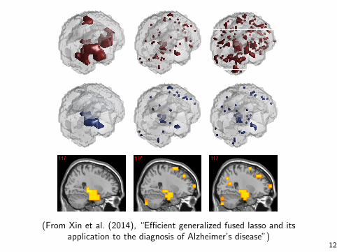
(a) fold 1 (b) fold 3 (c) fold 5 (d) fold 7 (e) fold 9 (f) overlap

Figure 4: Consistency of selected voxels in different trials of cross-validations. The results of 5 different folds of cross-validations are shownin (a)-(e) and the overlapping voxels in all 10 folds are shown in (f). The top row shows the results for GFL and the bottom row shows theresults for L1. The percentages of the overlapping voxels were: GFL(66%) vs. L1(22%).

Table 1: Comparison of the accuracy of AD classification.

Task LR SVM LR+L1 LR+GFLAD/NC 80.45% 82.71% 81.20% 84.21%

MCI 63.83% 67.38% 68.79% 70.92%

We compared GFL to logistic regression (LR), supportvector machine (SVM), and logistic regression with anL1 regularizer. The classification accuracies obtained basedon a 10-fold cross validation (CV) are shown in Table 1,which shows that GFL yields the highest accuracy in bothtasks. Furthermore, compared with other reported results,our performance are comparable with the state-of-the-art.In (Cheng, Zhang, and Shen 2012), the best performancewith MCI tasks is 69.4% but our method reached 70.92%.In (Chu et al. 2012), a similar sample size is used as in ourexperiments, the performance of our method with ADNCtasks is comparable to or better than their reported results(84.21% vs. 81-84%) whereas our performance with MCItasks is much better (70.92% vs. 65%).

We applied GFL to all the samples where the optimal pa-rameter settings were determined by cross-validation. Figure5 compares the selected voxels with non-structured sparsity(i.e. L1), which shows that the voxels selected by GFL clus-tered into several spatially connected regions, whereas thevoxels selected by L1 were more scattered. We consideredthe voxels that corresponded to the top 50 negative �i’s asthe most atrophied voxels and projected them onto a slice.The results show that the voxels selected by GFL were con-centrated in hippocampus, parahippocampal gyrus, whichare believed to be the regions with early damage that areassociated with AD. By contrast, L1 selected either less crit-ical voxels or noisy voxels, which were not in the regionswith early damage (see Figure 5(b) and 5(c) for details).The voxels selected by GFL were also much more consistentthan those selected by L1, where the percentages of overlap-ping voxels according to the 10-fold cross-validation were:

(a) (b) (c)

Figure 5: Comparison of GFL and L1. The top row shows theselected voxels in a 3D brain model, the middle row shows thetop 50 atrophied voxels, and the bottom row shows the projec-tion onto a brain slice. (a) GFL (accuracy=84.21%); (b) L1 (ac-curacy=81.20%); (c) L1 (similar number of voxels as in GFL).

GFL=66% vs. L1=22%, as shown in Figure 4.

ConclusionsIn this study, we proposed an efficient and scalable algo-rithm for GFL. We demonstrated that the proposed algo-rithm performs significantly better than existing algorithms.By exploiting the efficiency and scalability of the proposedalgorithm, we formulated the diagnosis of AD as GFL. Ourevaluations showed that GFL delivered state-of-the-art clas-sification accuracy and the selected critical voxels were wellstructured.

2168

(From Xin et al. (2014), “E�cient generalized fused lasso and itsapplication to the diagnosis of Alzheimer’s disease”)

12

Algorithms for the fused lasso

Let’s go through our toolset, to figure out how to solve

min

�f(�) + �kD�k1

Subgradient method: subgradient of criterion is

g = rf(�) + �DT�

where � 2 @kxk1 evaluated at x = D�, i.e.,

�i 2(

{sign

�(D�)i

�} if (D�)i 6= 0

[�1, 1] if (D�)i = 0

, i = 1, . . . m

Downside (as usual) is that convergence is slow. Upside is that g iseasy to compute (provided rf is): if S = supp(D�), then we let

g = rf(�) + �X

i2Ssign

�(D�)i

�· Di

13

Proximal gradient descent: prox operator is

proxt(�) = argmin

z

1

2tk� � zk22 + �kDzk1

This is not easy for a general di↵erence operator D (compare thisto soft-thresholding, if D = I). Prox itself is the fused lasso signalapproximator problem, with a Gaussian loss!

Could try reparametrizing the term kD�k1 to make it linear, whileintroducing inequality constraints. We could then apply an interiorpoint method

But we will have better luck going to the dual problem. (In fact, itis never a bad idea to look at the dual problem, even if you have agood approach for the primal problem!)

14

Fused lasso dual problem

Our problems are

Primal : min

�f(�) + �kD�k1

Dual : min

uf⇤

(�DTu) subject to kuk1 �

Here f⇤ is the conjugate of f . Note that u 2 Rm (where m is thenumber of rows of D) while � 2 Rn

The primal and dual solutions ˆ�, u are linked by KKT conditions:

rf(

ˆ�) + DT u = 0, and

ui 2

8><

>:

{�} if (D ˆ�)i > 0

{��} if (D ˆ�)i < 0

[��, �] if (D ˆ�)i = 0

, i = 1, . . . m

Second property implies that: ui 2 (��, �) =) (D ˆ�)i = 0

15

Let’s go through our toolset, to think about solving dual problem

min

uf⇤

(�DTu) subject to kuk1 �

Note the eventually we’ll need to solve rf(

ˆ�) = �DT u for primalsolution, and tractability of this depends on f

Proximal gradient descent: looks much better now, because prox is

proxt(u) = argmin

z

1

2tku � zk22 subject to kzk1 �

is easy. This is projection onto a box [��, �]

m, i.e., prox returns zwith

zi =

8><

>:

� if ui > �

�� if ui < ��

ui if ui 2 [��, �]

, i = 1, . . . m

16

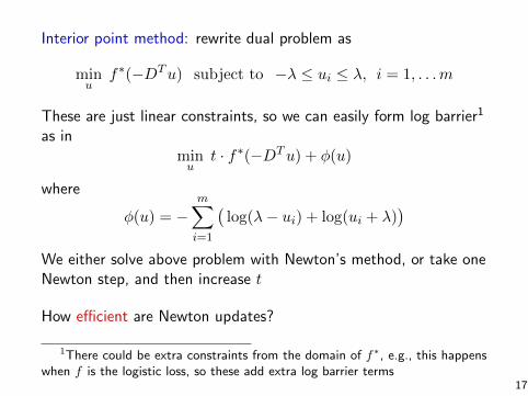
Interior point method: rewrite dual problem as

min

uf⇤

(�DTu) subject to �� ui �, i = 1, . . . m

These are just linear constraints, so we can easily form log barrier1

as inmin

ut · f⇤

(�DTu) + �(u)

where

�(u) = �mX

i=1

�log(� � ui) + log(ui + �)

�

We either solve above problem with Newton’s method, or take oneNewton step, and then increase t

How e�cient are Newton updates?

1There could be extra constraints from the domain of f⇤

, e.g., this happens

when f is the logistic loss, so these add extra log barrier terms

17

Define the barrier-smoothed dual criterion function

F (u) = tf⇤(�DTu) + �(u)

Newton updates follow direction H�1g, where

g = rF (u) = �t · D�rf⇤

(�DTu)

�+ r�(u)

H = r2F (u) = t · D�r2f⇤

(�DTu)

�DT

+ r2�(u)

How di�cult is it to solve a linear system in H?

• First term: if Hessian of the loss term r2f⇤(v) is structured,

and D is structured, then often Dr2f⇤(v)DT is structured

• Second term: Hessian of log barrier term r2�(u) is diagonal

So it really depends critically on first term, i.e., on conjugate lossf⇤ and penalty matrix D

18

Putting it all together:

• Primal subgradient method: iterations are cheap (we sum uprows of D over active set S), but convergence is slow

• Primal proximal gradient: iterations involve evaluating

proxt(�) = argmin

z

1

2tk� � zk22 + �kDzk1

which can be very expensive, convergence is medium

• Dual proximal gradient: iterations involve projecting onto abox, so very cheap, convergence is medium

• Dual interior point method: iterations involve a solving linearHx = g system in

H = t · D�r2f⇤

(�DTu)

�DT

+ r2�(u)

which may or may not be expensive, convergence is rapid

19

Reminder: conjugate functions

Recall that given f : Rn ! R, the function

f⇤(y) = max

x

yTx� f(x)

is called its conjugate

• Conjugates appear frequently in dual programs, since

�f⇤(y) = min

x

f(x)� yTx

• If f is closed and convex, then f⇤⇤= f . Also,

x 2 @f⇤(y) () y 2 @f(x) () x 2 argmin

z

f(z)� yT z

• If f is strictly convex f , then rf⇤(y) = argmin

z

f(z)� yT z

3

Dual (sub)gradient methods

What if we can’t derive dual (conjugate) in closed form, but wantto utilize dual relationship? Turns out we can still use dual-basedsubradient or gradient methods

Example: consider the problem

min

x

f(x) subject to Ax = b

Its dual problem is

max

u

�f⇤(�ATu)� bTu

where f⇤ is conjugate of f . Defining g(u) = f⇤(�ATu), note that

@g(u) = �A@f⇤(�ATu), and recall

x 2 @f⇤(�ATu) () x 2 argmin

z

f(z) + uTAz

5

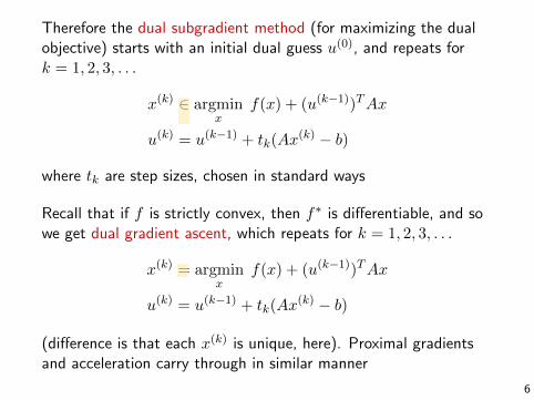
Therefore the dual subgradient method (for maximizing the dualobjective) starts with an initial dual guess u(0), and repeats fork = 1, 2, 3, . . .

x(k) 2 argmin

x

f(x) + (u(k�1))

TAx

u(k) = u(k�1)+ t

k

(Ax(k) � b)

where tk

are step sizes, chosen in standard ways

Recall that if f is strictly convex, then f⇤ is di↵erentiable, and sowe get dual gradient ascent, which repeats for k = 1, 2, 3, . . .

x(k) = argmin

x

f(x) + (u(k�1))

TAx

u(k) = u(k�1)+ t

k

(Ax(k) � b)

(di↵erence is that each x(k) is unique, here). Proximal gradientsand acceleration carry through in similar manner

6

Covergence analysis

First recall that if f strongly convex with parameter d, then rf⇤

Lipschitz with parameter 1/d

Proof: if f strongly convex and x is its minimizer, then

f(y) � f(x) +d

2

ky � xk2, for all y

Hence defining xu

= rf⇤(u), x

v

= rf⇤(v),

f(xv

)� uTxv

� f(xu

)� uTxu

+

d

2

kxu

� xv

k22

f(xu

)� vTxu

� f(xv

)� vTxv

+

d

2

kxu

� xv

k22

Adding these together, using Cauchy-Schwartz, and rearrangingshows that

kxu

� xv

k2 1

d· ku� vk2

7

Applying what we know about gradient descent: if f is stronglyconvex with parameter d, then dual gradient ascent with constantstep size t

k

d converges at rate O(1/✏)

Is this a slow or fast rate, compared to what we would get out ofprimal gradient descent? It’s actually essentially the same

• When f is strongly convex, primal gradient descent convergesat rate O(1/✏). But if we further assume that rf is Lipschitz,then we get the linear rate O(log(1/✏))

• Note: the converse of the statement on the last slide is alsotrue: rf⇤ being Lipschitz with parameter 1/d implies that fis strongly convex with parameter d

• Hence assume f⇤⇤= f . When f has Lipschitz gradient and is

strongly convex, the same is true about f⇤, and dual gradientascent also converges at the linear rate O(log(1/✏))

8

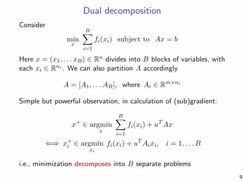
Dual decomposition

Consider

min

x

BX

i=1

fi

(xi

) subject to Ax = b

Here x = (x1, . . . xB) 2 Rn divides into B blocks of variables, witheach x

i

2 Rni . We can also partition A accordingly

A = [A1, . . . AB

], where Ai

2 Rm⇥ni

Simple but powerful observation, in calculation of (sub)gradient:

x+ 2 argmin

x

BX

i=1

fi

(xi

) + uTAx

() x+i

2 argmin

xi

fi

(xi

) + uTAi

xi

, i = 1, . . . B

i.e., minimization decomposes into B separate problems

9

Dual decomposition algorithm: repeat for k = 1, 2, 3, . . .

x(k)i

2 argmin

xi

fi

(xi

) + (u(k�1))

TAi

xi

, i = 1, . . . B

u(k) = u(k�1)+ t

k

⇣ BX

i=1

Ai

x(k)i

� b⌘

Can think of these steps as:

• Broadcast: send u to each ofthe B processors, eachoptimizes in parallel to find x

i

• Gather: collect Ai

xi

fromeach processor, update theglobal dual variable u

ux1

u x2 u x3

10

Example with inequality constraints:

min

x

BX

i=1

fi

(xi

) subject to

BX

i=1

Ai

xi

b

Dual decomposition (projected subgradient method) repeats fork = 1, 2, 3, . . .

x(k)i

2 argmin

xi

fi

(xi

) + (u(k�1))

TAi

xi

, i = 1, . . . B

v(k) = u(k�1)+ t

k

⇣ BX

i=1

Ai

x(k)i

� b⌘

u(k) = (v(k))+

where (·)+ is componentwise thresholding, (u+)i = max{0, ui

}

11

Augmented Lagrangian

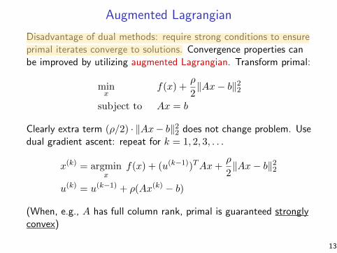
Disadvantage of dual methods: require strong conditions to ensureprimal iterates converge to solutions. Convergence properties canbe improved by utilizing augmented Lagrangian. Transform primal:

min

x

f(x) +⇢

2

kAx� bk22subject to Ax = b

Clearly extra term (⇢/2) · kAx� bk22 does not change problem. Usedual gradient ascent: repeat for k = 1, 2, 3, . . .

x(k) = argmin

x

f(x) + (u(k�1))

TAx+

⇢

2

kAx� bk22

u(k) = u(k�1)+ ⇢(Ax(k) � b)

(When, e.g., A has full column rank, primal is guaranteed stronglyconvex)

13

Notice step size choice tk

= ⇢, for all k, in dual gradient ascent.Why? Since x(k) minimizes f(x) + (u(k�1)

)

TAx+

⇢

2kAx� bk22over x, we have

0 2 @f(x(k)) +AT

⇣u(k�1)

+ ⇢(Ax(k) � b)⌘

= @f(x(k)) +ATu(k)

This is the stationarity condition for the original primal problem;can show under mild conditions that Ax(k) � b approaches zero(i.e., primal iterates approach feasibility), hence in the limit KKTconditions are satisfied and x(k), u(k) approach optimality

Advantage: much better convergence properties. Disadvantage:lose decomposability! (Separability is compromised by augmentedLagrangian ...)

14

Alternating direction method of multipliers

Alternating direction method of multipliers or ADMM: the best ofboth worlds!

I.e., good convergence properties of augmented Lagrangians, alongwith decomposability

Consider minimization problem

min

x

f1(x1) + f2(x2) subject to A1x1 +A2x2 = b

As before, we augment the objective

min

x

f1(x1) + f2(x2) +⇢

2

kA1x1 +A2x2 � bk22subject to A1x1 +A2x2 = b

15

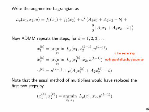
Write the augmented Lagrangian as

L⇢

(x1, x2, u) = f1(x1) + f2(x2) + uT (A1x1 +A2x2 � b) +⇢

2

kA1x1 +A2x2 � bk22

Now ADMM repeats the steps, for k = 1, 2, 3, . . .

x(k)1 = argmin

x1

L⇢

(x1, x(k�1)2 , u(k�1)

)

x(k)2 = argmin

x2

L⇢

(x(k)1 , x2, u

(k�1))

u(k) = u(k�1)+ ⇢(A1x

(k)1 +A2x

(k)2 � b)

Note that the usual method of multipliers would have replaced thefirst two steps by

(x(k)1 , x

(k)2 ) = argmin

x1,x2

L⇢

(x1, x2, u(k�1)

)

16

Convergence guarantees

Under modest assumptions on f1, f2 (these do not require A1, A2

to be full rank), the ADMM iterates satisfy, for any ⇢ > 0:

• Residual convergence: r(k) = A1x(k)1 �A2x

(k)2 � b ! 0 as

k ! 1, i.e., primal iterates approach feasibility

• Objective convergence: f1(x(k)1 ) + f2(x

(k)2 ) ! f?, where f? is

the optimal primal criterion value

• Dual convergence: u(k) ! u?, where u? is a dual solution

For details, see Boyd et al. (2010). Note that we do not genericallyget primal convergence, but this can be guaranteed under moreassumptions

Convergence rate: not known in general, theory is currently beingdeveloped, e.g., in Hong and Luo (2012), Nishihara et al. (2015).Roughly, it behaves like a first-order method (or a bit faster)

17

Scaled form

It is often easier to express the ADMM algorithm in a scaled form,where we replace the dual variable u by a scaled variable w = u/⇢.In this parametrization, the ADMM steps are

x(k)1 = argmin

x1

f1(x1) +⇢

2

kA1x1 +A2x(k�1)2 � b+ w(k�1)k22

x(k)2 = argmin

x2

f2(x2) +⇢

2

kA1x(k)1 +A2x2 � b+ w(k�1)k22

w(k)= w(k�1)

+A1x(k)1 +A2x

(k)2 � b

Note that here the kth iterate w(k) is just given by a running sumof residuals:

w(k)= w(0)

+

kX

i=1

�A1x

(i)1 +A2x

(i)2 � b

�

18

Practicalities and tricks

Practical experience shows that ADMM usually obtains a relativelyaccurate solution in a handful of iterations, but requires a verylarge number of iterations for a highly accurate solution. This ismore evidence that it behaves like a first-order method

Choice of ⇢ can greatly influence practical convergence of ADMM:

• ⇢ too large ! not enough emphasis on minimizing f1 + f2

• ⇢ too small ! not enough emphasis on feasibility

Boyd et al. (2010) give a strategy for varying ⇢ that can be usefulin practice (but does not have convergence guarantees)

Like deriving duals, transforming a problem into that ADMM canhandle often requires a bit of trickery (and di↵erent forms can leadto di↵erent algorithms)

19

Example: alternating projections

Consider finding a point in intersection of convex sets C,D ✓ Rn,i.e., solving

min

x

1

C

(x) + 1

D

(x)

To get this into ADMM form, we express it as

min

x,z

1

C

(x) + 1

D

(z) subject to x� z = 0

Each ADMM cycle involves two projections:

x(k) = argmin

x

PC

�z(k�1) � w(k�1)

�

z(k) = argmin

z

PD

�x(k) + w(k�1)

�

w(k)= w(k�1)

+ x(k) � z(k)

This is like the classical alternating projections method, but nowwith a dual variable w. It is more e�cient

20

Example: fused lasso regression

Given y 2 Rn, X 2 Rn⇥p, and a di↵erence operator D 2 Rm⇥p,the fused lasso regression problem solves

min

�2Rp

1

2

ky �X�k22 + �kD�k1

This computationally harder than the lasso problem (with D = I);recall our study on algorithms for this problem. We can rewrite as

min

�2Rp,↵2Rm

1

2

ky �X�k22 + �k↵k1 subject to D� � ↵ = 0

and ADMM gives us a simple algorithm for this problem:

�(k)= (XTX + ⇢DTD)

�1�XT y + ⇢DT

(↵(k�1) � w(k�1))

�

↵(k)= S

�/⇢

(D�(k)+ w(k�1)

)

w(k)= w(k�1)

+D�(k) � ↵(k)

21

Notes:

• The matrix XTX + ⇢DTD is assumed here to be invertible; ifnot, replace the inverse by a pseudoinverse

• If we take its factorization (say QR), in O(p3) flops, then eachsubsequent solve takes O(p2) flops

• The soft-thresolding operator St

recall is defined as

[St

(x)]j

=

8><

>:

xj

� t x > t

0 �t x t

xj

+ t x < �t

, j = 1, . . . p

• A di↵erent initial reparametrization, rather than D� = ↵, willlead to a di↵erent ADMM algorithm

• Sometimes it is more e�cient to make the substitution � = ↵in the penalty term; this is favorable when h(x) = kDxk1 hasa fast proximal operator

22

Consensus ADMM

Consider a problem of the form

min

x

BX

i=1

fi

(x)

The consensus ADMM approach begins by reparametrizing:

min

x1,...xB ,x

BX

i=1

fi

(xi

) subject to xi

= x, i = 1, . . . B

and this yields the decomposable ADMM updates:

x(k)i

= argmin

xi

fi

(xi

) +

⇢

2

kxi

� x(k�1)+ w

(k�1)i

k22, i = 1, . . . B

x(k) =1

B

BX

i=1

⇣x(k)i

+ w(k�1)i

⌘

w(k)i

= w(k�1)i

+ x(k)i

� x(k), i = 1, . . . B

25

Write x =

1B

PB

i=1 xi and similarly for other variables. Not hard to

see that w(k)= 0 for all iterations k � 1

Hence ADMM steps can be simplified, by taking x(k) = x(k):

x(k)i

= argmin

xi

fi

(xi

) +

⇢

2

kxi

� x(k�1)+ w

(k�1)i

k22, i = 1, . . . B

w(k)i

= w(k�1)i

+ x(k)i

� x(k), i = 1, . . . B

To reiterate, the xi

, i = 1, . . . B updates here are done in parallel

Intuition:

• We try to minimize each fi

(xi

), and use ridge regularizationto pull each x

i

towards the average x

• If a variable xi

is bigger than the average, then wi

is increased

• So the ridge regularization in the next step pulls xi

even closer

26

General consensus ADMM with regularization

Consider a problem of the form

min

x

BX

i=1

fi

(aTi

x+ bi

) + g(x)

For consensus ADMM, we again reparametrize:

min

x1,...xB ,x

BX

i=1

fi

(aTi

xi

+ bi

) + g(x) subject to xi

= x, i = 1, . . . B

and this yields the decomposable ADMM updates:

x(k)i

= argmin

xi

fi

(aTi

xi

+ bi

) +

⇢

2

kxi

� x(k�1)+ w

(k�1)i

k22,

i = 1, . . . B

x(k) = argmin

x

B⇢

2

kx� x(k) � w(k�1)k22 + g(x)

w(k)i

= w(k�1)i

+ x(k)i

� x(k), i = 1, . . . B

27

Notes:

• It is no longer true that w(k)= 0, so ADMM steps do not

simplify as before

• To reiterate, the xi

, i = 1, . . . B are done in parallel

• Each xi

, i = 1, . . . B can be thought of as a loss minimizationon part of the data, with ridge regularization

• The x update is a proximal operation in regularizer g

• The w update drives the individual variables into consensus

• A di↵erent initial reparametrization (i.e., changing xi

= x,i = 1, . . . B to say, aT

i

xi

+ bi

= x, i = 1, . . . B) will lead to adi↵erent ADMM algorithm

See Boyd et al. (2010) for more details about consensus ADMM,implementation tips, and more advanced strategies for splitting upinto di↵erent subproblems

28

Q&A!Thanks!