Understanding the Convergence of the AlternatingDirection Method of Multipliers: Theoretical and

Computational Perspectives ∗

Jonathan Eckstein† Wang Yao‡

October 20, 2015

Abstract

The alternating direction of multipliers (ADMM) is a form of augmented Lagrangianalgorithm that has experienced a renaissance in recent years due to its applicabilityto optimization problems arising from “big data” and image processing applications,and the relative ease with which it may be implemented in parallel and distributedcomputational environments. While it is easiest to describe the method as an ap-proximate version of the classical augmented Lagrangian algorithm, using one pass ofblock coordinate minimization to approximately minimize the augmented Lagrangianat each iteration, the known convergence proofs bear no discernible relationship to thisdescription. In this largely tutorial paper, we try to give an accessible version of the“operator splitting” version of the ADMM convergence proof, first developing someanalytical tools that we also use to analyze a simple variant of the classical augmentedLagrangian method. We assume relatively little prior knowledge of convex analysis.Using two dissimilar classes of application problems, we also computationally comparethe ADMM to some algorithms that do indeed work by approximately minimizing theaugmented Lagrangian. The results suggest that the ADMM is different from suchmethods not only in its convergence analysis but also in its computational behavior.

This paper is an expanded and revised version of Optimization Online working paper2012.12.3704. An abridged version is slated to appear in Pacific Journal of Optimization.

1 Introduction

The alternating direction method of multipliers (ADMM) is a convex optimization algorithmfirst proposed in 1975 [17, page 69] and first analyzed in the early 1980’s [15, 16]. It hasattracted renewed attention recently due to its applicability to various machine learning andimage processing problems. In particular,

∗This work was partially supported by National Science Foundation grant CCF-1115638.†Department of Management Science and Information Systems and RUTCOR, Rutgers University, 100

Rockafeller Road, Piscataway, NJ (jeckstei@rci.rutgers.edu).‡RUTCOR, Rutgers University, 100 Rockafeller Road, Piscataway, NJ (wang.yao09@rutgers.edu).

1

• It appears to perform reasonably well on these relatively recent applications, betterthan when applied to traditional operations research problems such as minimum-costnetwork flows.

• The ADMM can take advantage of the structure of these problems, which involveoptimizing sums of fairly simple but sometimes nonsmooth convex functions.

• Extremely high accuracy is not usually a requirement for these applications, reducingthe impact of the ADMM’s tendency toward slow “tail convergence”.

• Depending on the application, it is often relatively easy to implement the ADMMin a distributed-memory, parallel manner. This property is important for “big data”problems in which the entire problem dataset may not fit readily into the memory ofa single processor.

The recent survey article [6] describes the ADMM from the perspective of machine learningapplications; another, older survey is contained in the doctoral thesis [9].

Although it can be developed in a slightly more general form — see for example [6] —the following problem formulation is sufficient for most applications of the ADMM:

minx∈Rn

f(x) + g(Mx). (1)

Here, M is an m×n matrix, often assumed to have full column rank, and f and g are convexfunctions on Rn and Rm, respectively. We let f and g take not only values in R but also thevalue +∞, so that constraints may be “embedded” in them, in the sense that if f(x) = ∞or g(Mx) =∞, then the point x is considered to be infeasible for (1).

By appropriate use of infinite values for f or g, a very wide range of convex problems maybe modeled through (1). To make the discussion more concrete, however, we now describe asimple illustrative example that fits readily into the form (1) without use of infinite functionvalues, and resembles in basic structure of many of the applications responsible for theresurgence of interest in the ADMM: the “lasso” or “compressed sensing” problem. Thisproblem takes the form

minx∈Rn

12‖Ax− b‖2 + ν ‖x‖1 , (2)

where A is a p × n matrix, b ∈ Rp, and ν > 0 is a given scalar parameter. The idea of thismodel is find an approximate solution to the linear equations Ax = b, but with a preferencefor making the solution vector x ∈ Rn sparse; the larger the value of the parameter ν, themore the model prefers sparsity of the solution versus accuracy of solving Ax = b. While thismodel has some limitations in terms of finding sparse near-solutions to Ax = b, it serves as agood example application for the ADMM, simply by taking f(x) = 1

2‖Ax− b‖2, M = I, and

g(x) = ν ‖x‖1. Many other now-popular applications have a similar general form, but mayuse more complicated norms in place of ‖ · ‖1; for example, in some applications, x is treatedas a matrix, and one uses the nuclear norm (the sum of singular values) in the objective totry to induce x to have low rank.

We now describe the classical augmented Lagrangian method and the ADMM for (1).First, note that we can rewrite (1), introducing an additional decision variable vector z ∈ Rm,

2

as the following problem over x ∈ Rn and z ∈ Rm:

min f(x) + g(z)ST Mx = z.

(3)

For this formulation, the classical augmented Lagrangian algorithm, which we will discussin more depth in Section 3, takes the form

(xk+1, zk+1) ∈ Arg minx∈Rn,z∈Rm

{f(x) + g(z) + 〈λk,Mx− z〉+ ck

2‖Mx− z‖2} (4)

λk+1 = λk + ck(Mxk+1 − zk+1). (5)

Here, {λk} is a sequence of estimates of the Lagrange multipliers of the constraints Mx = z,while {(xk, zk)} is a sequence of estimates of the solution vectors x and z, and {ck} is asequence of positive scalar parameters bounded away from 0. Throughout this article, 〈a, b〉denotes the usual Euclidean inner product a>b.

In this setting, the standard augmented Lagrangian algorithm (4)-(5) is not very attrac-tive because the minimizations of f and g in the subproblem (4) are strongly coupled throughthe term ck

2‖Mx− z‖2, and hence the subproblems are not likely to be easier to solve than

the original problem (1).The alternating direction method of multipliers (ADMM) for (1) or (3) takes the following

form, for some scalar parameter c > 0:

xk+1 ∈ Arg minx∈Rn

{f(x) + g(zk) + 〈λk,Mx− zk〉+ c

2

∥∥Mx− zk∥∥2}

(6)

zk+1 ∈ Arg minz∈Rm

{f(xk+1) + g(z) + 〈λk,Mxk+1 − z〉+ c

2

∥∥Mxk+1 − z∥∥2}

(7)

λk+1 = λk + c(Mxk+1 − zk+1). (8)

Clearly, the constant terms g(zk) and f(xk+1), as well as some other constants, may bedropped from the respective minimands of (6) and (7). Unlike the classical augmentedLagrangian method, the ADMM essentially decouples the functions f and g, since (6) requiresonly minimization of a quadratic perturbation of f , and (7) requires only minimization of aquadratic perturbation of g. In many situations, this decoupling makes it possible to exploitthe individual structure of the f and g so that each of (6) and (7) may be computed in anefficient and perhaps highly parallel manner.

Given the form of the two algorithms, it is natural to view the ADMM (6)-(8) as anapproximate version of the classical augmented Lagrangian method (4)-(5) in which a singlepass of “Gauss-Seidel” block minimization substitutes for full minimization of the augmentedLagrangian Lc(x, z, λ

k), where we define

Lc(x, z, λ) = f(x) + g(z) + 〈λ,Mx− z〉+ c2‖Mx− z‖2. (9)

That is, we substitute minimization with respect to x followed by minimization with respectto z for the joint minimization with respect to x and z required by (4). This viewpoint wasin fact the motivation for the original proposal for the ADMM in [17]. Curiously, however,this interpretation does not seem to play a role in any known convergence proof for the

3

ADMM, and there is no known general way of quantifying how closely one iteration of thetwo calculations (6)-(7) approaches the joint minimization (4).

There are two fundamental approaches to proving the convergence of the ADMM, eachbased on a different form of two-way splitting, that is, expressing a mapping as the sumof two simpler mappings. One approach is at its core based on a splitting of the classicalLagrangian function

L(x, z, λk) = f(x) + g(z) + 〈λk,Mx− z〉 (10)

of the problem (3). This approach dates back to [15], and essentially equivalent analyseswere given later, for example, in the textbook [5] and the appendix to the survey article [6].The drawback of this approach is that the analysis is quite lengthy and its structure can behard to discern.

The second convergence proof approach for the ADMM dates back to [16], and is basedon combining a splitting of the dual functional of (3) with some operator splitting theoryoriginating in [27]. This approach is elaborated and expanded in the popular reference [11],and it can be made simpler and more intuitive using ideas from [26]. Once understood, theoperator-splitting perspective yields considerable insight into the convergence of the ADMM.Its existing presentations, however, require considerable background in convex analysis andcan thus be somewhat unapproachable.

This article has two goals: the first is to attempt to convey the understanding inher-ent in the second, operator-splitting approach to proving convergence of the ADMM, butassuming only basic knowledge of convex analysis. To this end, some mathematical rigorwill be sacrificed in the interest of clarifying the key concepts. The intention is to makemost of the benefits of a deeper understanding of the method available to a widest possibleaudience — in essence, the idea is to simplify the analysis of [16, 11] into a form that doesnot require extensive convex analysis background, developing the required concepts in thesimplest required form as the analysis proceeds.

The second goal of this article is to present some recent computational results whichillustrate that the convergence theory of the ADMM also seems to have a practical dimen-sion. In particular, these results suggest that, despite outward appearances and its originalmotivation, significant insight is missing if we primarily think of the ADMM as an approx-imate version of the the classical augmented Lagrangian algorithm using block coordinateminimization for the subproblems. In particular, using two different problems classes, wecomputationally compare the ADMM to methods that are in fact approximate augmentedLagrangian algorithms with block-coordinate-minimization subproblem solvers, and showthat they have significantly different behavior.

The remainder of this article is structured as follows: Section 2 summarizes some nec-essary background material, which may be largely skipped by readers familiar with convexanalysis. Section 3 presents the classic augmented Lagrangian method for convex problemsas an application of nonexpansive algorithmic mappings, and then Section 4 applies the sameanalytical techniqeus to the ADMM. Section 5 describes a simple way of adapting the ADMMto problems with more than just two objective components f and g. Section 6 presents thecomputational results, while Section 7 makes some concluding remarks and presents someavenues for future research. The material in Sections 2-4 is not fundamentally new, and canbe inferred from the references mentioned in each section; the only contribution is in the

4

manner of presentation. The new computational work underscores the ideas found in thetheory and raises some issues for future investigation. Finally, the algorithm of Section 5seems to be periodically forgotten and rediscovered; it is also described in Section 5.2 of thetextbook [4].

2 Background Material from Convex Analysis

This section summarizes some basic analytical results that will help to structure and clarifythe following analysis. Proofs are only included when they are simple and insightful. Morecomplicated proofs will be either sketched or omitted. Most of the material here can bereadily found (often in more general form) in [30] or in textbooks such as [2, 3]. Themain insight meant to be provided by this section is that there is a strong relationshipbetween convex functions and nonexpansive mappings, that is, functions N : Rn → Rn with‖N(x)−N(x′)‖ ≤ ‖x− x′‖ for all x, x′ ∈ Rn. Furthermore, in the case of particular kindsof convex functions d arising from dual formulations of optimization problems, there is arelatively simple way to evaluate the nonexpansive map N that corresponds to d.

Definition 1 Given any function f : Rn → R ∪ {+∞} a vector v ∈ Rn is said to be asubgradient of f at x ∈ Rn if

f(x′) ≥ f(x) + 〈v, x′ − x〉 ∀x′ ∈ Rn. (11)

The notation ∂f(x) denotes the set of all subgradients of f at x.

Essentially, v is a subgradient of f at x if the affine function a( · ) given by a(x′) =f(x) + 〈v, x′−x〉 underestimates f throughout Rn. Furthermore, it can be seen immediatelyfrom the definition that x∗ is a global minimizer of f if and only if 0 ∈ ∂f(x∗). If f isdifferentiable at x and convex, then ∂f(x) is the singleton set {∇f(x)} (this fact is intuitiveto visualize, but the proof is nontrivial; see for example [30, 3]). Convergence proofs forconvex optimization algorithms very frequently use the following property of the subgradient:

Lemma 2 The subgradient mapping of a function f : Rn → R ∪ {+∞} has the followingmonotonicity property: given any x, x′, v, v′ ∈ Rn such that v ∈ ∂f(x) and v′ ∈ ∂f(x′), wehave

〈x− x′, v − v′〉 ≥ 0. (12)

Proof. From the subgradient inequality (11), we have f(x′) ≥ f(x) + 〈v, x′ − x〉 and f(x) ≥f(x′) + 〈v′, x− x′〉, which we may add to obtain

f(x) + f(x′) ≥ f(x) + f(x′) + 〈v − v′, x′ − x〉.

Canceling the identical terms f(x)+f(x′) from both sides and rearranging yields (12). �

From this monotonicity property, it is simple to derive a basic “decomposition” propertyof subgradients, which is a basic building block of the ADMM convergence proof we willexplore in the next section:

5

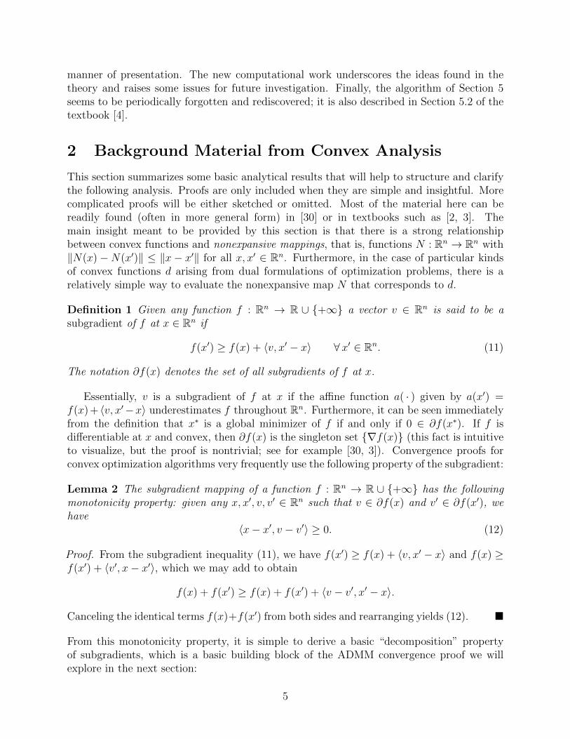
Lemma 3 Given any function f : Rn → R ∪ {+∞}, a vector z ∈ Rn, and a scalar c > 0there is at most one way to write z = x+ cv, where v ∈ ∂f(x).

Proof. Suppose that y = x + cv = x′ + cv′ where v ∈ ∂f(x) and v′ ∈ ∂f(x′). Then simplealgebra yields x−x′ = c(v′−v) and hence 〈x−x′, v−v′〉 = −c‖v − v′‖2. But since Lemma 2asserts that 〈x− x′, v − v′〉 ≥ 0, we must have v = v′ and hence x = x′. �

x cv z

1(0, )zc

( ,0)z

( , )x v

Figure 1: Graphical depiction of Lemmas 2 and 3 for dimension n = 1.

Figure 1 shows a simplified depiction of Lemmas 2 and 3 in R1. The solid line illustratesthe set of pairs (x, v) ∈ Rn × Rn for which v ∈ ∂f(x); by Lemma 2, connecting any twosuch pairs must result in a line segment that is either vertical or has nonnegative slope. Thedashed line represents the set of points (x, v) ∈ Rn×Rn satisfying x+ cv = z; since this linehas negative slope, it can intersect the solid line at most once, illustrating Lemma 3. Next,we give conditions under which a decomposition of any z ∈ Rn into x+ cv, v ∈ ∂f(x) mustexist, in addition to having to be unique. First, we state a necessary background result:

Lemma 4 Suppose f : Rn → R ∪ {+∞} and g : Rn → R are convex, and g is continuouslydifferentiable. Then, at any x ∈ Rn,

∂(f + g)(x) = ∂f(x) +∇g(x) = {y +∇g(x) | y ∈ ∂f(x)} .

The proof of this result is somewhat more involved than one might assume, so we omit it;see for example [30, Theorem 23.8 and 25.1] or [3, Propositions 4.2.2 and 4.2.4]. However,the result itself should be reasonably intuitive: adding a differentiable convex function g tothe convex function f simply translates the set of subgradients at each point x by ∇g(x).

Definition 5 A function f : Rn → R ∪ {+∞} is called proper if it is not everywhere +∞,that is, there exists x ∈ Rn such that f(x) ∈ R. Such a function is called closed if the set{(x, t) ∈ Rn × R | t ≥ f(x)} is closed.

6

By a straightforward argument, it may be seen that closedness of f is equivalent to the lowersemicontinuity condition that f(limk→∞ x

k) ≤ lim infk→∞ f(xk) for all convergent sequences{xk} ⊂ Rn; see [30, Theorem 7.1] or [3, Proposition 1.2.2]. We are now ready to state asimple condition guaranteeing that a decomposition of the form given in Lemma 3 must existfor every z ∈ Rn.

Proposition 6 If f : Rn → R ∪ {+∞} is closed, proper, and convex, then for any scalarc > 0, each point z ∈ Rn can be written in exactly one way as x+ cv, where v ∈ ∂f(x).

Sketch of proof. Let c > 0 and z ∈ Rn be given. Consider now the function f : Rn →R∪ {+∞} given by f(x) = f(x) + 1

2c‖x− z‖2. Using the equivalence of closedness to lower

semicontinuity, it is easily seen that f being closed and proper implies that f is closed andproper. The convex function f can decrease with at most a linear rate in any direction, so thepresence of the quadratic term 1

2c‖x− z‖2 guarantees that f is coercive, that is f(x)→ +∞

as ‖x‖ → ∞. Since f is proper, closed, and coercive, one can then invoke a version of theclassical Weirstrass theorem — see for example [3, Proposition 2.1.1] — to assert that fmust attain its minimum value at some point x, which implies that 0 ∈ ∂f(x). Since f andx 7→ 1

2c‖x− z‖2 are both convex, and the latter is differentiable, Lemma 4 asserts that there

must exist v ∈ ∂f(x) such that 0 = v + ∇x

(12c‖x− z‖2 ) = v + 1

c(x − z), which is easily

rearranged into z = x+cv. Lemma 3 asserts that this representation must be unique. �

This result is a special case of Minty’s theorem [29]. We now show that, because of themonotonicity of the subgradient map, we may construct a nonexpansive mapping on Rn

corresponding to any closed proper convex function:

Proposition 7 Given a closed proper convex function f : Rn → R ∪ {+∞} and a scalarc > 0, the mapping Ncf : Rn → Rn given by

Ncf (z) = x− cv where x, v ∈ Rn are such that v ∈ ∂f(x) and x+ cv = z (13)

is everywhere uniquely defined and nonexpansive. The fixed points of Ncf are precisely theminimizers of f .

Proof. From Proposition 6, there is exactly one way to express any z ∈ Rn as x + cv, soNcf (z) exists and is uniquely defined for all z ∈ Rn. To show that Ncf is nonxpansive,consider any any z, z′ ∈ Rn, respectively expressed as z = x + cv and z′ = x′ + cv′ withv ∈ ∂f(x) and v′ ∈ ∂f(x′). Then we write

‖z − z′‖2= ‖x+ cv − (x′ + cv′)‖2

= ‖x− x′‖2+ 2c〈x− x′, v − v′〉+ c2 ‖v − v′‖2

‖Ncf (z)−Ncf (z′)‖2

= ‖x− cv − (x′ − cv′)‖2

= ‖x− x′‖2 − 2c〈x− x′, v − v′〉+ c2 ‖v − v′‖2.

Therefore,‖Ncf (z)−Ncf (z

′)‖2= ‖z − z′‖2 − 4c〈x− x′, v − v′〉.

7

By monotonicity of the subgradient, the inner product in the last term is nonnegative, leadingto the conclusion that ‖Ncf (z)−Ncf (z

′)‖ ≤ ‖z − z′‖. With z, x, and v as above, we notethat

Ncf (z) = z ⇔ x− cv = x+ cv ⇔ v = 0 ⇔ x minimizes f and z = x.

This equivalence proves the assertion regarding fixed points. �

We now show one additional consequence of closedness which will be needed later.

Lemma 8 If f is a closed convex function and {xk}, {vk} ⊂ Rn are convergent sequencessuch that vk ∈ ∂f(xk) for all k, then limk→∞ v

k ∈ ∂f(limk→∞ x

k).

Proof. Let x∞ = limk→∞ xk and v∞ = limk→∞ v

k. For any x′ ∈ Rn we have

f(x′) ≥ f(xk) + 〈vk, x′ − xk〉.

Taking limits as k →∞, we obtain

f(x′) ≥ lim supk→∞

f(xk) + 〈v∞, x′ − x∞〉.

Since f is closed, lim infk→∞ f(xk) ≥ f(x∞). So, substituting f(x∞) ≤ lim infk→∞ f(xk) ≤lim supk→∞ f(xk) into the above inequality, we obtain

f(x′) ≥ f(x∞) + 〈v∞, x′ − x∞〉,

which, since the choice of x′ is arbitrary, implies that v∞ ∈ ∂f(x∞). �

3 The Classical Augmented Lagrangian Method and

Nonexpansiveness

We now review the theory of the classical augmented Lagrangian method from the standpointof nonexpansive mappings; although couched in slightly different language here, this analysisoriginated with [32, 33]. Consider an optimization problem

min h(x)ST Ax = b,

(14)

where h : Rn → R ∪ {+∞} is closed proper convex, and Ax = b represents an arbitraryset of linear inequality constraints. This formulation can subsume the problem (3) throughthe change of variables (x, z) → x, letting b = 0 ∈ Rm and A = [M − I], and defining happropriately.

Using standard Lagrangian duality1, the dual function of (14) is

q(λ) = minx∈Rn{h(x) + 〈λ,Ax− b〉} . (15)

1Rockafellar’s parametric conjugate duality framework [31] gives deeper insight into the material presentedhere, but in order to focus on the main topic at hand, we use a form of duality that should be more familiarto most readers.

8

The dual problem to (14) is to maximize q(λ) over λ ∈ Rm. Defining d(λ) = −q(λ), we mayequivalently formulate the dual problem as minimizing the function d over Rm. We nowconsider the properties of the negative dual function d:

Lemma 9 The function d is closed and convex. If the vector x∗ ∈ Rn attains the minimumin (15) for some given λ ∈ Rm, then b− Ax∗ ∈ ∂d(λ).

Proof. We have that d(λ) = maxx∈Rn{−h(x)− 〈λ,Ax− b〉}, that is, that d is the pointwisemaximum, over all x ∈ Rn, of the affine (and hence convex) functions of λ given by ax(λ) =−h(x)− 〈λ,Ax− b〉. Thus, d is convex, and

{(λ, t) ∈ Rm × R | t ≥ d(λ)} =⋂x∈Rn

{(λ, t) ∈ Rm × R | t ≥ −h(x)− 〈λ,Ax− b〉} .

Each of the sets on the right of this relation is defined by a single non-strict linear inequalityon (λ, t) and is thus closed. Since any intersection of closed sets is also closed, the set on theleft is also closed and therefore d is closed.

Next, suppose that x∗ attains the minimum in (15). Then, for any λ′ ∈ Rm,

q(λ′) = minx∈Rn{h(x) + 〈λ′, Ax− b〉}

≤ h(x∗) + 〈λ′, Ax∗ − b〉= h(x∗) + 〈λ,Ax∗ − b〉+ 〈λ′ − λ,Ax∗ − b〉= q(λ) + 〈Ax∗ − b, λ′ − λ〉.

Negating this relation yields d(λ′) ≥ d(λ) + 〈b− Ax∗, λ′ − λ〉 for all λ′ ∈ Rm, meaning thatb− Ax∗ ∈ ∂d(λ). �

Since d is closed, then if it is also proper, that is, it is finite for at least one choice ofλ ∈ Rm, Proposition 6 guarantees that any µ ∈ Rm can be decomposed into µ = λ + cv,where v ∈ ∂d(λ). A particularly interesting property of functions defined like d is that thisdecomposition may be computed in a manner not much more burdensome than evaluatingd itself:

Proposition 10 Given any µ ∈ Rm, consider the problem

minx∈Rn{h(x) + 〈µ,Ax− b〉+ c

2‖Ax− b‖2}. (16)

If x is an optimal solution to this problem, setting λ = µ+ c(Ax− b) and v = b−Ax yieldsλ, v ∈ Rm such that λ+ cv = µ and v ∈ ∂d(λ), where d = −q is as defined above.

Proof. Appealing to Lemma 4, x is optimal for (16) if there exists w ∈ ∂h(x) such that

0 = w + ∂∂x

[〈µ,Ax− b〉+ c

2‖Ax− b‖2]

x=x

= w + A>µ+ cA>(Ax− b)= w + A>

(µ+ c(Ax− b)

)= w + A>λ,

where λ = µ+ c(Ax− b) as above. Using Lemma 4 once again, this condition means that xattains the minimum in (15), and hence Lemma 9 implies that v = b−Ax ∈ ∂d(λ). Finally,we note that λ+ cv = µ+ c(Ax− b) + c(b− Ax) = µ. �

9

For a general closed proper convex function, computing the decomposition guaranteed toexist by Proposition 6 may be much more difficult than simply evaluating the function. Themain message of Proposition 10 is that for functions d obtained from the duals of convexprogramming problems like (14), this may not be the case — it may be possible to computethe decomposition by solving a minimization problem that could well be little more difficultthan required to evaluate d itself. To avoid getting bogged down in convex-analytic detailsthat would distract from our main goals, we will not directly address here exactly when it isguaranteed that an optimal solution to (16) exists; we will simply assume that the problemhas a solution. This situation is also easily verified in most applications.

Since the decomposition µ = λ + cv, v ∈ ∂d(λ), can be evaluated by solving (16), thesame calculation allows us to evaluate the nonexpansive mapping Ncd, using the notation ofSection 2: specifically, using the notation of Proposition 10, we have

Ncd(µ) = λ− cv = µ+ c(Ax− b)− c(b− Ax) = µ+ 2c(Ax− b).

We know that Ncd is a nonexpansive map, and that any fixed point of Ncd is a minimizer ofd, that is, an optimal solution to the dual problem of (14). It is thus tempting to considersimply iterating the map λk+1 = Ncd(λ

k) recursively starting from some arbitrary λ0 ∈ Rm

in the hope that {λk} would converge to a fixed point. Now, if we knew that the Lipschitzmodulus of Ncd were less than 1, linear convergence of λk+1 = Ncd(λ

k) to such a fixed pointwould be elementary to establish. However, we only know that the Lipschitz modulus ofNcd is at most 1. Thus, if we were to iterate the mapping λk+1 = Ncd(λ

k), it is possible theiterates could simply “orbit” at fixed distance from the set of fixed points without converging.

We now appeal to a long-established result from fixed point theory, which asserts thatif one “blends” a small amount of the identity with a nonexpansive map, convergence isguaranteed and such “orbiting” cannot occur:

Theorem 11 Let T : Rm → Rm be nonexpansive, that is, ‖T (y)− T (y′)‖ ≤ ‖y − y′‖ for ally, y′ ∈ Rm. Let the sequence {ρk} ⊂ (0, 2) be such that infk{ρk} > 0 and supk{ρk} < 2. Ifthe mapping T has any fixed points and {yk} conforms to the recursion

yk+1 = ρk2T (yk) + (1− ρk

2)yk, (17)

then {yk} converges to a fixed point of T .

Proof. This proof is a simplification of the one given for a slightly stronger result in Theorem5.14 of [2]. Suppose y∗ is any fixed point of T . Then, for any k ≥ 0,∥∥yk+1 − y∗

∥∥2=∥∥ρk

2T (yk) + (1− ρk

2)yk − y∗

∥∥2

=∥∥ρk

2(T (yk)− y∗) + (1− ρk

2)(yk − y∗)

∥∥2

=(ρk2

)2 ∥∥T (yk)− y∗∥∥2

+(1− ρk

2

)2 ∥∥yk − y∗∥∥2

+ 2(ρk2

) (1− ρk

2

)〈T (yk)− y∗, yk − y∗〉

10

=(ρk2

)2 ∥∥T (yk)− y∗∥∥2

+(1− ρk

2

)2 ∥∥yk − y∗∥∥2

+ 2(ρk2

) (1− ρk

2

)〈T (yk)− y∗, yk − y∗〉

+(ρk2

) (1− ρk

2

) ∥∥T (yk)− yk∥∥2

−(ρk2

) (1− ρk

2

) ∥∥T (yk)− yk∥∥2

=(ρk2

)2 ∥∥T (yk)− y∗∥∥2

+(1− ρk

2

)2 ∥∥yk − y∗∥∥2

+ 2(ρk2

) (1− ρk

2

)〈T (yk)− y∗, yk − y∗〉

+(ρk2

) (1− ρk

2

) (∥∥T (yk)− y∗∥∥2 − 2〈T (yk)− y∗, yk − y∗〉+

∥∥yk − y∗∥∥2)

−(ρk2

) (1− ρk

2

) ∥∥T (yk)− yk∥∥2

=(ρk2

) ∥∥T (yk)− y∗∥∥2

+(1− ρk

2

) ∥∥yk − y∗∥∥2 −(ρk2

) (1− ρk

2

) ∥∥T (yk)− yk∥∥2

=(ρk2

) ∥∥T (yk)− T (y∗)∥∥2

+(1− ρk

2

) ∥∥yk − y∗∥∥2 −(ρk2

) (1− ρk

2

) ∥∥T (yk)− yk∥∥2

≤(ρk2

) ∥∥yk − y∗∥∥2+(1− ρk

2

) ∥∥yk − y∗∥∥2 −(ρk2

) (1− ρk

2

) ∥∥T (yk)− yk∥∥2

=∥∥yk − y∗∥∥2 −

(ρk2

) (1− ρk

2

) ∥∥T (yk)− yk∥∥2

Here, the inequality follows from the nonexpansiveness of T , and the preceding equalityholds because y∗ is a fixed point of T . By the assumption on {ρk}, there exists some ε > 0such that

(ρk2

) (1− ρk

2

)≥ ε for all k, so∥∥yk+1 − y∗

∥∥2 ≤∥∥yk − y∗∥∥2 − ε

∥∥T (yk)− yk∥∥2

(18)

for all k. Adding this relation from k = 0 to k = K − 1, we obtain that for any K ≥ 0 wehave ∥∥yK − y∗∥∥2 ≤

∥∥y0 − y∗∥∥2 − ε

K−1∑k=0

∥∥T (yk)− yk∥∥2.

It follows that {yk} is a bounded sequence and {T (yk) − yk} must form a summable se-ries, hence T (yk) − yk → 0. Being bounded, {yk} must possess at least one limit point.Considering any such limit point y∞ and a corresponding subsequence of indices K withyk →K y∞, we note that by the (Lipschitz) continuity of T , we must have T (y∞) − y∞ =limk→∞,k∈K

{T (yk)− yk

}, which we know to be 0 since the entire sequence {T (yk) − yk}

converges to zero. Hence T (y∞) = y∞ and y∞ is a fixed point of T . This makes it possibleto substitute y∗ = y∞ into (18), from which we conclude that

∥∥yk+1 − y∞∥∥ ≤ ∥∥yk − y∞∥∥ for

all k. Since y∞ is a limit point of {yk}, it follows that yk → y∞, and we already know y∞ tobe a fixed point of T . �

The case ρk = 1 in the above result corresponds to taking the simple average 12T + 1

2I of T

with the identity map. The ρk ≡ 1 case of Theorem 11 was proven, in an infinite-dimensionalsetting, as long ago as 1955 [25].

Combining Proposition 10 and Theorem 11 yields a convergence proof for a form ofaugmented Lagrangian algorithm:

11

Proposition 12 Consider a problem of the form (14) and a scalar c > 0. Suppose, forsome scalar sequence {ρk} ⊂ (0, 2) with the property that infk{ρk} > 0 and supk{ρk} < 2,the sequences {xk} ⊂ Rn and {λk} ⊂ Rm evolve according to the recursions

xk+1 ∈ Arg minx∈Rm

{h(x) + 〈λk, Ax− b〉+ c

2‖Ax− b‖2} (19)

λk+1 = λk + ρkc(Axk+1 − b). (20)

If the dual problem to (14) possesses an optimal solution, then {λk} converges to one ofthem, and all limit points of {xk} are optimal solutions to (14).

Proof. The optimization problem solved in (19) is just the one in Proposition 10 with λk

substituted for µ. Therefore,

Ncd(λk) = λk + c(Axk+1 − b)− c(b− Axk+1) = λk + 2c(Axk+1 − b),

and consequently

ρk2Ncd(λ

k) + (1− ρk2

)λk = ρk2

(λk + 2c(Axk+1 − b)

)+ (1− ρk

2)λk

= λk + ρkc(Axk+1 − b),

meaning that λk+1 = ρk2Ncd(λ

k) + (1 − ρk2

)λk. An optimal solution to the dual of (14) is aminimizer of d, and hence a fixed point of Ncd by Proposition 7. Theorem 11 then impliesthat {λk} converges to such a fixed point.

Since λk is converging and {ρk} is bounded away from 0, we may infer from (20) thatAxk− b→ 0. If x∗ is any optimal solution to (14), we have from Ax∗ = b and the optimalityof xk+1 in (19) that

h(xk+1) + 〈λk+1, Axk+1 − b〉+ c2

∥∥Axk+1 − b∥∥2

≤ h(x∗) + 〈λk+1, Ax∗ − b〉+ c2‖Ax∗ − b‖2 = h(x∗),

that is, h(xk) + 〈λk−1, Axk − b〉+ c2‖Axk − b‖2 ≤ h(x∗) for all k. Let x∞ be any limit point

of {xk}, and K denote a sequence of indices such that xk →K x∞. Since Axk − b → 0, wehave Ax∞ = b. Since h is closed, it is lower semicontinuous, so

h(x∞) ≤ lim infk→∞k∈K

h(xk) = lim infk→∞k∈K

{h(xk) + 〈λk−1, Axk − b〉+ c

2‖Axk − b‖

}≤ h(x∗),

and so x∞ is also optimal for (14). �

There are two differences between (19)-(20) and the augmented Lagrangian method asit is typical presented for (14). First, many versions of the augmented Lagrangian methodomit the parameters {ρk}, and are thus equivalent to the special case ρk ≡ 1. Second, itis customary to let the parameter c vary from iteration to iteration, replacing it with asequence of parameters {ck}, with infk{ck} > 0. In this case, one cannot appeal directlyto the classical fixed-point result of Theorem 11 because the operators Nckd being used ateach iteration may be different. However, essentially the same convergence proof as forTheorem 11 may still be employed, because the operators Nckd all have exactly the samefixed points, namely the set of optimal dual solutions. This observation, in a more generalform, is the essence of the convergence analysis of the proximal point algorithm [32, 33]; seealso [11].

12

4 Analyzing the ADMM through Compositions of

Nonexpansive Mappings

We now describe the convergence theory of the ADMM (6)-(8) using the same basic toolsdescribed in the previous section. Essentially, this material is a combination and simplifiedoverview of analyses of the ADMM and related methods in such references as [27], [16], [26],[9], and [12, Section 1]; a similar treatment may be found in [11].

To begin, we consider the dual of the problem (3), namely to maximize the function

q(λ) = minx∈Rn

z∈Rm

{f(x) + g(z) + 〈λ,Mx− z〉} (21)

= minx∈Rn{f(x) + 〈λ,Mx〉}+ min

z∈Rm{g(z)− 〈λ, z〉} (22)

= q1(λ) + q2(λ), (23)

where we define

q1(λ) = minx∈Rn{f(x) + 〈λ,Mx〉} q2(λ) = min

z∈Rm{g(z)− 〈λ, z〉} . (24)

Defining d1(λ) = −q1(λ) and d2(λ) = −q2(λ), the dual of (3) is thus equivalent to minimizingthe sum of the two convex functions d1 and d2:

minλ∈Rm

d1(λ) + d2(λ) (25)

The functions d1 and d2 have the same general form as the dual function d of the previoussection; therefore, we can apply the same analysis:

Lemma 13 The functions d1 and d2 are closed and convex. Given some λ ∈ Rm, supposex∗ ∈ Rn attains the first minimum in (24). Then −Mx∗ ∈ ∂d1(λ). Similarly, if z∗ ∈ Rp

attains the second minimum in (24), then z∗ ∈ ∂d2(λ).

Proof. We simply apply Lemma 9 twice. In the case of d1, we set h = f , A = M , and b = 0,while in the case of d2, we set h = g, A = −I, and b = 0. �

We now consider some general properties of problems of the form (25), that is, minimizingthe sum of two convex functions.

Lemma 14 A sufficient condition for λ∗ ∈ Rm to solve (25) is that

there exists v∗ ∈ ∂d1(λ∗) such that − v∗ ∈ ∂d2(λ∗). (26)

Proof. For all λ ∈ Rm the subgradient inequality gives

d1(λ) ≥ d1(λ∗) + 〈v∗, λ− λ∗〉d2(λ) ≥ d2(λ∗) + 〈−v∗, λ− λ∗〉.

Adding these two inequalities produces the relation d1(λ) + d2(λ) ≥ d1(λ∗) + d2(λ∗) for allλ ∈ Rm, so λ∗ must be optimal for (25). �

13

Under some mild regularity conditions that are met in most practical applications, (26) isalso necessary for optimality; however, to avoid a detour into subdifferential calculus, we willsimply assume that this condition holds for at least one optimal solution λ∗ of (25).

Fix any constant c > 0 and assume that d1 and d2 are proper, that is, each is finite for atleast one value of the argument λ. Since d1 and d2 are closed and convex, we may concludethat they correspond to nonexpansive maps as shown in Section 2. These maps are given by

Ncd1(y) = λ− cv where λ, v ∈ Rm are such that v ∈ ∂d1(λ) and λ+ cv = y

Ncd2(y) = µ− cw where µ,w ∈ Rm are such that w ∈ ∂d2(µ) and µ+ cw = y.

Ncd1 and Ncd2 are both nonexpansive by the analysis given in Section 3. It follows that theirfunctional composition Ncd1 ◦Ncd2 is also nonexpansive, that is,∥∥Ncd1

(Ncd2(y)

)−Ncd1

(Ncd2(y

′))∥∥ ≤ ‖Ncd2(y)−Ncd2(y

′)‖ ≤ ‖y − y′‖

for all y, y′ ∈ Rm. We now consider the set of fixed points of this composed mapping:

Lemma 15 The set of fixed points of the map Ncd1 ◦Ncd2 is

fix(Ncd1 ◦Ncd2) = {λ+ cv | v ∈ ∂d2(λ),−v ∈ ∂d1(λ)} .

Proof. Take any y ∈ Rm and write it as y = λ + cv, where v ∈ ∂d2(λ); Lemma 13 andProposition 6 imply that this must be possible. Then Ncd2(y) = λ − cv. Now, again usingLemma 13 and Proposition 6, we know that Ncd2(y) = λ− cv can be written in exactly oneway as µ+ cw, where w ∈ ∂d1(µ). Then Ncd1(Ncd2(y)) = µ− cw, and thus y is a fixed pointof Ncd1 ◦Ncd2 if and only if

µ− cw = y = λ+ cv. (27)

Adding µ + cw = Ncd2(y) = λ− cv to (27), we obtain µ = λ. Substituting µ = λ into (27),we also obtain w = −v. �

Thus, finding a fixed point of Ncd1 ◦ Ncd2 is essentially the same as finding two vectorsλ, v ∈ Rm satisfying v ∈ ∂d2(λ), −v ∈ ∂d1(λ), and thus an optimal solution to the dualproblem (25). Finding such a point essentially results in finding a solution to the prob-lem (3), as we now show. We first make one standard definition regarding the solution,and a regularity assumption that will play the role of standard constraint qualification (acondition guaranteeing the existence of a Lagrange multiplier).

Definition 16 A KKT point for problem (3) is some((x∗, z∗), λ∗

)∈ (Rn ×Rn)×Rm such

that

1. x∗ minimizes f(x) + 〈λ∗,Mx〉 with respect to x

2. z∗ minimizes g(z)− 〈λ∗, z〉 with respect to z

3. Mx∗ = z∗.

Assumption 17 All subgradients of the function d1(λ) = minx∈Rn{f(x) + 〈λ,Mx〉} at eachpoint λ ∈ Rm take the form −Mx, where x attains the stated minimum over x in (24).

14

We note that Lemma 9 guarantees that −Mx is subgradient of d1 at λ whenever x minimizesf(x) + 〈λ∗,Mx〉 over x, so the assumption merely says that there are no other subgradients.This assumption is guaranteed by a variety of more standard regularity conditions that aremet in most practical applications. However, to avoid getting sidetracked in convex-analyticdetails, we keep the assumption as stated.

Lemma 18 If((x∗, z∗), λ∗

)is a KKT point, then (x∗, z∗) is an optimal solution of (3) and

x∗ is an optimal solution of (1). If Assumption 17 holds and z∗ ∈ ∂d2(λ∗) and −z∗ ∈ ∂d1(λ∗),then there exists x∗ ∈ Rn such that

((x∗, z∗), λ∗

)is a KKT point.

Proof. Consider the first statement. Conditions 1 and 2 of the KKT point definition im-ply that (x∗, z∗) minimize problem (3)’s classical Lagrangian L(x, z, λ∗) over (x, z). KKTcondition 3 states that (x∗, z∗) is also feasible for the problem constraints. Since the prob-lem is convex, (x∗, z∗) is an optimal solution. It immediately follows that x∗ is optimal forproblem (1). Now consider the second statement, and let (z, λ) be as hypothesized. If As-sumption 17 holds, there must exist some x∗ ∈ Rn minimizing f(x) + 〈λ∗,Mx〉 over x suchthat −Mx∗ = −z∗. �

At this point, an obvious strategy is to try to apply Theorem 11 to finding a fixed pointof Ncd1 ◦Ncd2 , leading essentially immediately to a solution of (25). That is, we perform theiteration

yk+1 = ρk2Ncd1

(Ncd2(y

k))

+ (1− ρk2

)yk (28)

for some sequence of parameters {ρk} with infk{ρk} > 0 and supk{ρk} < 2.We now show that this procedure turns out to be equivalent to the ADMM. We show

this equivalence in two stages, first by converting (28) into a more computationally explicitbut still generic form, and then specializing this form to our particular form of d1 and d2.To begin the first stage of this analysis, consider the point yk at the beginning of such aniteration, and express it as λk + cvk, for vk ∈ ∂d2(λk). Then, to apply the recursion (28), weproceed as follows:

1. Applying the map Ncd2 produces the point λk − cvk.

2. Next, we express λk − cvk as µk + cwk, for wk ∈ ∂d1(µk).

3. We then calculate

yk+1 = ρk2Ncd1(Ncd2(y

k)) + (1− ρk2

)yk

= ρk2Ncd1(µ

k + cwk) + (1− ρk2

)(λk + cvk)

= ρk2

(µk − cwk) + (1− ρk2

)(λk + cvk).

Finally, the last expression for yk+1 above may be simplified as follows: since we know

15

λk − cvk = µk + cwk, we have by simple rearrangement that λk − µk = c(vk + wk). Thus,

yk+1 = ρk2

(µk − cwk) + (1− ρk2

)(λk + cvk)

= ρk2

(µk − cwk − (λk + cvk)

)+ λk + cvk

= ρk2

(µk − λk − c(vk + wk)

)+ λk + cvk

= ρk2

(2(µk − λk)

)+ λk + cvk

= ρkµk + (1− ρk)λk + cvk,

where the second-to-last equality follows from λk − µk = c(vk + wk). Thus, in terms of thesequences {λk}, {µk}, {vk}, and {wk}, the algorithm may be expressed as follows, startingfrom some arbitrary λ0, v0 ∈ Rm:

1. Find µk, wk such that wk ∈ ∂d1(µk) and

µk + cwk = λk − cvk. (29)

2. Find λk+1, vk+1 such that vk+1 ∈ ∂d2(λk+1) and

λk+1 + cvk+1 = ρkµk + (1− ρk)λk + cvk. (30)

We know in this situation that the vectors yk = λk+1 + cvk+1 should converge to a point ofthe form y∗ = λ∗ + cv∗, where v∗ ∈ ∂d2(λ∗) and −v∗ ∈ ∂d1(λ), meaning that λ∗ solves (25).As an aside, this pattern of computations is an example of (generalized) Douglas-Rachfordsplitting [27, 9, 11], whose relationship to the ADMM was first shown in [16]. Douglas-Rachford splitting is the same basic “engine” behind the convergence of several other popularalgorithms, including the progressive hedging method for stochastic programming [34].

We now move to the second stage of our derivation, in which we specialize the scheme (29)-(30) above to the particular functions d1 = −q1 and d2 = −q2, where q1 and q2 are definedby (24). Conveniently, we can simply apply Proposition 10: in the case of (29) with d1 = −q1,applying Proposition 10 with h = f , A = M , b = 0, and µ = λk−cvk yields the computation

xk+1 ∈ Arg minx∈Rn

{f(x) + 〈λk − cvk,Mx〉+ c

2‖Mx‖2} (31)

µk = λk − cvk + cMxk+1 (32)

wk = −Mxk+1. (33)

Now let us consider (30), with d2 = −q2: again applying Proposition 10, but now with h = g,A = −I, b = 0, and µ = ρkµ

k + (1− ρk)λk + cvk, yields the computation

zk+1 ∈ Arg minx∈Rn

{g(z) + 〈ρkµk + (1− ρk)λk + cvk,−z〉+ c

2‖−z‖2} (34)

λk+1 = ρkµk + (1− ρk)λk + cvk − czk+1 (35)

vk+1 = zk+1. (36)

16

We now simplify the system of recursions (31)-(36). First, we note that the sequence {wk}does not appear explicitly except in (33), so we may simply eliminate it. Second, using (36),we may substitute vk = zk throughout, yielding

xk+1 ∈ Arg minx∈Rn

{f(x) + 〈λk − czk,Mx〉+ c

2‖Mx‖2} (37)

µk = λk − czk + cMxk+1 (38)

zk+1 ∈ Arg minx∈Rn

{g(z)− 〈ρkµk + (1− ρk)λk + czk, z〉+ c

2‖z‖2} (39)

λk+1 = ρkµk + (1− ρk)λk + czk − czk+1. (40)

Next, consider (37). Adding the constant c2‖zk‖2 to the minimand and completing the square

yields the equivalent computation

xk+1 ∈ Arg minx∈Rn

{f(x) + 〈λk,Mx〉+ c

2

∥∥Mx− zk∥∥2}

(41)

From (38), we have µk = λk + c(Mxk+1 − zk), hence

ρkµk + (1− ρk)λk + czk = ρk

(λk + c(Mxk+1 − zk)

)+ (1− ρk)λk + czk

= λk + ρkcMxk+1 + (1− ρk)czk

= λk + c(ρkMxk+1 + (1− ρk)zk

). (42)

Thus, the minimand in (39) may be written

g(z)− 〈λk + c(ρkMxk+1 + (1− ρk)zk

), z〉+ c

2‖z‖2 .

Similarly to the derivation of (41), adding the constant c2‖ρkMxk+1 + (1− ρk)zk‖2 and com-

pleting the square yields the equivalent minimand

g(z)− 〈λk, z〉+ c2

∥∥ρkMxk+1 + (1− ρk)zk − z∥∥2,

and substituting (42) into (40) produces

λk+1 = λk + c(ρkMxk+1 + (1− ρk)zk − zk+1

).

Summarizing, the recursions (31)-(36) collapse to

xk+1 ∈ Arg minx∈Rn

{f(x) + 〈λk,Mx〉+ c

2

∥∥Mx− zk∥∥2}

(43)

zk+1 ∈ Arg minz∈Rp

{g(z)− 〈λk, z〉+ c

2

∥∥ρkMxk+1 + (1− ρk)zk − z∥∥2}

(44)

λk+1 = λk + c(ρkMxk+1 + (1− ρk)zk − zk+1

). (45)

In the special case ρk ≡ 1, these recursions reduce exactly to the ADMM (6)-(8), except forsome immaterial constant terms in the minimands.

This derivation contains the essence of the operator-splitting convergence theory of theADMM method: it is an application of the fixed-point algorithm of Theorem 11 to thenonexpansive mapping Ncd1 ◦ Ncd2 . We take advantage of this observation in the followingproposition:

17

Proposition 19 Let the constant c > 0 be given and suppose that Assumption 17 holds andthere exists a KKT point for problem (3). Then if the sequences {xk} ⊂ Rn, {zk} ⊂ Rm,and {λk} ⊂ Rm conform to the recursions (43)-(45), where infk{ρk} > 0 and supk{ρk} < 2,we have that λk → λ∗, zk → z∗, and Mxk → Mx∗ = z∗, where

((x∗, z∗), λ∗

)is some KKT

point.

Proof. The development above shows that the recursions (43)-(45) are equivalent to thesequence yk = λk+cvk = λk+czk being produced by the recursion (28), which by Theorem 11converges to a fixed point of the operator Ncd1 ◦Ncd2 , if one exists. The existence of such afixed point is implied by Lemma 18 and the hypothesis that a KKT point exists. Thereforeyk is convergent to some fixed point y∞ of Ncd1 ◦ Ncd2 , which by Lemma 15 is of the formy∞ = λ∞ + cz∞, where z∞ ∈ ∂d2(λ∞) and −z∞ ∈ ∂d1(λ∞). By the assumption regardingd1, there exists some x∞ such that −Mx∞ = −z∞, that is, Mx∞ = z∞.

Consider the mapping Pcd2 = 12Ncd2 + 1

2I. Since Ncd2 is nonexpansive, Pcd2 is certainly

continuous. We have Pcd2(y∞) = 1

2(λ∞− cz∞) + 1

2(λ∞+ cz∞) = λ∞ and similarly Pcd2(y

k) =λk since zk = vk ∈ ∂d2(λk), and so by the continuity of Pcd2 we must have λk = Pcd2(y

k)→Pcd2(y

∞) = λ∞ and thus zk = 1c(yk − λk)→ 1

c(y∞− λ∞) = z∞. We may also rewrite (45) as

λk+1 − λk = cρk(Mxk+1 − zk) + c(zk − zk+1). (46)

The quantity on the left of (46) converges to 0 since {λk} is convergent, while the last termon the right converges to 0 since {zk} is convergent. Since ρk is bounded away from 0, itfollows that Mxk+1 → z∞ = Mx∞. �

There are a number of observations worth making at this point:

1. In most results regarding the convergence of the ADMM, Assumption 17 is typicallyreplaced by more natural, verifiable assumptions regarding f and M ; these assumptionsimply that Assumption 17 holds, and are met in almost all practical applications. Theversion of the analysis given above was chosen to minimize the amount of convex-analytical background required.

2. The ADMM’s convergence analysis is not based on approximating the nonexpansivemapping Ncd = Nc(d1+d2) underlying the classical method of multipliers as applied toproblem (3), but on exact evaluation of the related but fundamentally different nonex-pansive mapping Ncd1 ◦Ncd2 . From a theoretical standpoint, therefore, the ADMM isnot an approximate version of the classical augmented Lagrangian method. Note thatapproximate versions of the ADMM are possible, as described for example in [11].

3. Varying the parameter c from one iteration to another is more problematic for theADMM than for the classical augmented Lagrangian method, because changing c shiftsthe set of fixed points of the map Ncd1 ◦Ncd2 . This phenomenon makes proving the con-vergence of the ADMM with nonconstant c much more difficult, although some partialresults have been obtained; see for example [22] (or [1], for a specific application).

4. The technique of composing Ncd1 with Ncd2 to obtain a nonexpansive mapping whosefixed points are closely related to the minimizers of d1 + d2 does not have an obvious

18

extension to the case of more than two functions: for example, if we consider threeconvex functions d1, d2, d3, the fixed points of Ncd1 ◦Ncd2 ◦Ncd3 are not closely relatedto the minima of d1 + d2 + d3. This phenomenon helps explain the relative difficulty ofproving the convergence of the ADMM when extended in a direct manner to more thantwo blocks of variables. The beginning of Section 5 below discusses such extensions inmore detail.

5. Here, we are essentially following the operator splitting approach to analyzing the con-vergence of the ADMM, as first explored in [16]. When one follows this approach,the overrelaxation parameters ρk appear in a different way than in the classical aug-mented Lagrangian method. Applying the augmented Lagrangian method (19)-(20) tothe problem formulation (3) results in a version of the method (4)-(5) in which (5) isamended to

λk+1 = λk + ρkck(Mxk+1 − zk+1). (47)

On the other hand, ρk is used in a different way in (43)-(45): the overrelaxationparameter appears in the “target” value ρkMxk+1+(1−ρk)zk for z in (44) and similarlyin the following multiplier update (45).

6. As mentioned earlier, there is another approach to proving the convergence of theADMM, which dates back to [15] and is based on a splitting of the Lagrangian func-tion (10), rather than a splitting of the dual function. This path of analysis leadsto a convergence proof which, instead of being based on the Fejer monotonicity of{λk + czk} to the set fix(Ncd1 ◦ Ncd2) = {λ+ cv | v ∈ ∂d2(λ),−v ∈ ∂d1(λ)}, estab-lishes Fejer monotonicity of {(λk, czk)} to the set {(λ, cv) | v ∈ ∂d2(λ),−v ∈ ∂d1(λ)},which is a slightly different condition. When this approach is taken, the overrelax-ation parameters ρk naturally appear only in the multiplier update, and one obtains amethod consisting of (6), (7), and (47), that is,

xk+1 ∈ Arg minx∈Rn

{f(x) + 〈λk,Mx〉+ c

2

∥∥Mx− zk∥∥2}

(48)

zk+1 ∈ Arg minz∈Rm

{g(z)− 〈λk, z〉+ c

2

∥∥Mxk+1 − z∥∥2}

(49)

λk+1 = λk + ρkck(Mxk+1 − zk+1). (50)

The analysis in [15] proves convergence of this method, where ρk is constant andin the range

(0, (1 +

√5)/2

); the same proof can be easily generalized to the case

0 < lim infk→∞ ρk ≤ lim supk→∞ ρk < (1 +√

5)/2. This is a narrower range for {ρk}than one obtains for the operator-splitting-based analysis, and furthermore it does notappear that there is any way to derive the method (48)-(50) from the operator-splittingapproach presented in this paper.2 Technically, this result means there are actuallytwo distinct families of ADMM algorithms, one derived from the operator-splittingframework and the other derived from Lagrangian splitting. These two families co-incide in the case ρk ≡ 1, in which case (43)-(45) and (48)-(50) become identical

2Specifically, to derive (48) from the operator-splitting framework, one needs zk ∈ ∂d2(λk), but choosingρk 6= 1 in the previous iteration’s execution of (50) violates this condition.

19

sequences of calculations. Which form of overrelaxation is preferable in practice ap-pears to depend on the application. This paper has explored the operator-splittingframework, because its conceptual structure is easier to understand and yields moreintuition about the algorithm. However, some of the same insights can be gleanedfrom the Lagranian-splitting framework. For example, in the Lagrangian-splittingapproach, it is apparent that changing the value of c shifts the set of fixed points{(λ, cv) | v ∈ ∂d2(λ),−v ∈ ∂d1(λ)} that attracts the iterates, which helps explain thedifficulties of proving convergence for variable c. And again, the proof is not basedon one pass of the computations (6)-(7) measurably approximating overall minimiza-tion of the augmented Lagrangian, but on establishing Fejer monotonicity to some setrelated to the optimality conditions v ∈ ∂d2(λ), −v ∈ ∂d1(λ).

5 Adapting the ADMM to More than Two Blocks of

Variables

It is natural to consider adapting the ADMM to problems similar to (3), but involving morethan two functions. Consider the problem

min

p∑i=1

fi(xi)

ST

p∑i=1

Aixi = b,

(51)

where xi denotes a vector in Rni , each fi is a closed proper convex function Rni → R∪{+∞},each Ai is an ni ×m matrix, and b ∈ Rm.

One obvious extension of the ADMM to this problem form is to form the augmentedLagrangian of (51) and construct an algorithmic loop consisting of the following steps:

• Minimize the augmented Lagrangian with respect to x1, holding the remaining xiconstant

• Minimize the augmented Lagrangian with respect to x2, holding the remaining xiconstant

...

• Minimize the augmented Lagrangian with respect to xp, holding the remaining xiconstant

• Perform a standard Lagrange multiplier update.

Unfortunately, no convergence proof is known this algorithm for p > 2, and although itappears to to work well in many practical examples, the recent working paper [7] constructsa p = 3 example in which it diverges. The p > 2 case is an area of active research — see forexample [18, 19, 20, 21, 23]. Some authors augment the basic pattern above with “corrector”steps that permit proofs of convergence; the algorithm in [14] could also be used to derive

20

such a method. Others [23] impose additional strong assumptions and restrictions on themethod, such as a very small limit on ρk in (50).

An alternative approach to the pattern above is to reformulate (51) into the form (3),and then apply the ADMM directly. One way of doing so is to let

x = (x1, . . . , xp) ∈ Rn1 × · · · × Rnp = R(∑p

i=1 ni)

z = (z1, . . . , zp) ∈ Rm × · · · × Rm = Rpm

f(x) =

p∑i=1

fi(xi)

M =

A1

A2

. . .

Ap

g(z) =

{0, if

∑pi=1 zi = b,

+∞, otherwise.

With these choices of f , g, and M , problems (1) and (3) are easily seen to be equivalentto (51). In this case, the associated Lagrange multiplier vector λ is also in Rpm, so we willwrite it as (λ1, . . . , λp), where λ1, . . . , λp ∈ Rm (however, we will soon see that it is possibleto condense this representation).

Let us consider applying the ADMM to this choice of f , g, and M . First, the x-minimization step (6) takes the form

xk+1 ∈ Arg min

x∈R(∑pi=1

ni)

{p∑i=1

(fi(xi) + 〈λki , Aixi − zki 〉+ c

2

∥∥Aixi − zki ∥∥2)}

.

This minimization decomposes into p separate problems, one for each value of i, so we mayequivalently write

xk+1i ∈ Arg min

xi∈Rni

{fi(xi) + 〈λki , Aixi − zki 〉+ c

2

∥∥Aixi − zki ∥∥2}

i = 1, . . . , p. (52)

Next, we consider the z-minimization step (7), which does not decompose in the same man-ner. Instead, we have

zk+1 = (zk+11 , . . . , zk+1

p ) ∈ Arg min∑p

i=1

(〈λki , Aixk+1

i − zi〉+ c2

∥∥Aixk+1i − zi

∥∥2)

ST∑p

i=1 zi = b.

Completing the square in the objective function, an equivalent problem is

zk+1 = (zk+11 , . . . , zk+1

p ) ∈ Arg min∑p

i=1

(c2

∥∥1cλki + Aix

k+1i − zi

∥∥2)

ST∑p

i=1 zi = b.

In Rpm, this is simply the problem of projecting the point

uk = (uk1, . . . , ukp) =

(1cλk1 + A1x

k+11 , 1

cλk2 + A2x

k+12 , . . . , 1

cλkp + Apx

k+1p

)21

onto the affine subspace given by∑p

i=1 zi = b. A straightforward analysis of the form ofthe orthogonal linear subspace, or an equivalent Lagrange multiplier analysis, shows thatthis projection can be performed by simply subtracting the same vector dk ∈ R from eachuki = 1

cλki + Aix

k+1i in such a way that

∑pi=1(uki − dk) = b. The vector dk that has this

property is easily seen to be

dk = 1p

(p∑i=1

ui − b

)= 1

p

(p∑i=1

(1cλki + Aix

k+1i

)− b

). (53)

Finally, we consider the multiplier update (8). Using the definition of M , we note that theupdate λk+1 = λk + c(Mxk+1 − zk+1) takes the form, for each i = 1, . . . , p, of

λk+1i = λki + c(Aix

k+1i − zk+1

i )

= λki + c(Aix

k+1i − (uki − dk)

)= λki + c(Aix

k+1i − uki + dk)

= λki + c(Aix

k+1i −

(1cλki + Aix

k+1i

)+ dk

)= cdk

Thus, except possibly for their initial values for k = 0, the subvectors λki of the Lagrangemultiplier vector λk = (λk1, . . . , λ

kp) are all identical. If we constrain this to be the case for

k = 0 as well, we may thus write them as λk ∈ Rm and substitute λk for λki and dk = 1cλk+1 in

all the formulas above. Performing these substitutions in (53) and then multiplying throughby c yields the simplified multiplier update

λk+1 = λk +c

p

(p∑i=1

Aixk+1i − b

)= λk −

(c

p

)rk+1, (54)

where we define the constraint residual rk to be(∑p

i=1 Aixki

)− b for all k. Making the same

substitutions in the calculation of zk+1i , we have

zk+1i = uki − dk

=(

1cλki + Aix

k+1i

)− 1

cλk+1

=(

1cλk + Aix

k+1i

)− 1

cλk+1

= Aixk+1i − 1

c

(λk+1 − λk

)= Aix

k+1i − 1

c

((c

p

)rk+1

)[from (54)]

= Aixk+1i − (1

p)rk+1.

Combining this expression for zki with (52), (54), and the definition of rk, we conclude that

22

the ADMM takes the equivalent complete form

xk+1i ∈ Arg min

xi∈Rni

{fi(xi) + 〈λk, Aixi − zki 〉+ c

2

∥∥Aixi − zki ∥∥2}

i = 1, . . . , p (55)

rk+1 =

(p∑i=1

Aixki

)− b (56)

zk+1i = Aix

k+1i − (1

p)rk i = 1, . . . , p (57)

λk+1 = λk −(c

p

)rk+1, (58)

with the Lagrange multiplier estimates λk now in Rm. For large values of p, this algorithmhas the advantage of being almost completely parallel: one processor can be assigned toeach value of the index i, and if one replicates the vectors rk and λk on every processor,one can perform the computations (55), (57), and (58) completely simultaneously on allprocessors. The only interprocessor communication required at each step is the global sumoperation in the calculation of the residual (56). This kind of global vector summationis a very common operation in parallel computing, and can typically be performed veryefficiently. Thus, for large values of p, parallelism considerations may make this simplereformulation of the ADMM to handle problem (51) preferable to variants that process thevarious components fi of the objective function in a sequential manner. The only potentialproblem is that the presence of p in the denominator in the multiplier update (58) may makemultiplier adjustments slow for large p, but many more complicated ADMM-like methodsshare similar potential drawbacks. This algorithm could also be accelerated by incorporationof an overrelaxation factor ρ. For ρ = 1, as we have developed here, this algorithm isalso discussed in the upcoming textbook [4]; unfortunately, it was omitted from the widelyreferenced tutorial paper [6].

6 Computational Comparison of the ADMM and Ap-

proximate Augmented Lagrangian Methods

6.1 Comparison Algorithms

The preceding sections have attempted to give some theoretical insight into the the differencesbetween the classical augmented Lagrangian algorithm and the ADMM. Both may be viewedas applications of the same basic result about convergence of iterated nonexpansive mappings,but in significantly different ways: despite outward appearances, the ADMM is not from theexisting theoretical perspective an approximate version of the augmented Lagrangian methodusing a single pass of a block-minimization method to approximately minimize the augmentedLagrangian. We now explore the same topic from a computational perspective by comparingthe ADMM to methods that really do perform measurable approximate minimization of theaugmented Lagrangian.

One difficulty with approximate augmented Lagrangian algorithms is that they can in-volve approximation criteria — that is, conditions for deciding whether one is sufficiently

23

close to having found a minimum of subproblems such as (4) or (19) — that can be hard totest in practice. Notable exceptions are the methods proposed in [10, 13]. Here, we will focuson the “relative error” method of [13], which appears to have the best practical performancein the prior literature; we will not review or explain the analysis of these methods here.

In the context of problem (14), each iteration of the algorithmic template of [13] takesthe following general form, where σ ∈ [0, 1) is a fixed parameter:

1. Find xk+1, yk+1 ∈ Rn such that

yk ∈ ∂x[h(x) + 〈λk, Ax− b〉+ ck

2‖Ax− b‖2]

x=xk+1 (59)

2ck

∣∣〈wk − xk+1, yk〉∣∣+ ‖yk‖2 ≤ σ

∥∥Axk+1 − b∥∥2

(60)

2. Perform the updates

λk+1 = λk + ck(Axk+1 − b) (61)

wk+1 = wk − ckyk. (62)

In (59), ∂x denotes the set of subgradients with respect to x, with λ treated as a fixedparameter. The conditions (59)-(60) constitute an approximate minimization with respectto x, in the sense that if xk+1 exactly minimizes the augmented Lagrangian as in (19),then we can take yk = 0 and (60) is immediately satisfied because its left-hand side is zeroand its right-hand side must be nonnegative. However, (59)-(60) can tolerate a less exactminimization, with a subgradient that is not exactly 0. Note that {yk}, {wk} ⊂ Rn areauxiliary sequences that are not needed in the exact form of the algorithm.

Adapting this pattern to the specific problem (1), we split yk into (ykx, ykz ) ∈ Rn × Rm

and similarly split wk into (wkx, wkz ) ∈ Rn×Rm, obtaining the following recursive conditions,

where we use the augmented Lagrangian notation Lc defined in (9):

(ykx, ykz ) ∈ ∂(x,z)Lc(x

k+1, zk+1, λk) (63)

2ck

∣∣∣〈wkx − xk+1, ykx〉+ 〈wkz − zk+1, ykz 〉∣∣∣+ ‖ykx‖2 + ‖ykz‖2 ≤ σ

∥∥Mxk+1 − zk+1∥∥2

(64)

λk+1 = λk + ck(Mxk+1 − zk+1) (65)

wk+1x = wkx − ckykx (66)

wk+1z = wkz − ckykz . (67)

We now consider how to perform the approximate minimization embodied in (63)-(64),keeping in mind that f or g (or both) might be nonsmooth; for example, in the lassoproblem (2), the function f is smooth, but g is nonsmooth.

As suggested at least as long ago as in [17], one way to attempt to approximately mini-mize the augmented Lagrangian is to use a block Gauss-Seidel algorithm which alternatelyminimizes with respect to x and then with respect to z, that is (looping over i),

xk,i+1 ∈ Arg minx∈Rn

{Lck(x, zk,i, pk)

}(68)

zk,i+1 ∈ Arg minz∈Rm

{Lck(xk,i+1, z, pk)

}(69)

24

Repeat for i = 0, 1, . . .

xk,i+1 ∈ Arg minx∈Rn

{Lck(x, zk,i, λk)

}zk,i+1 ∈ Arg min

z∈Rm

{Lck(xk,i+1, z, λk)

}Until there exists yk ∈ ∂xLck(xk,i, zk,i, λk) with

2ck

∣∣〈wk − xk,i, yk〉∣∣+ ‖yk‖2 ≤ σ‖Mxk,i − zk,i‖2

λk+1 = λk + ρkck(Mxk,i − zk,i)wk+1 = wk − ckyk

xk+1,0 = xk,i

zk+1,0 = zk,i

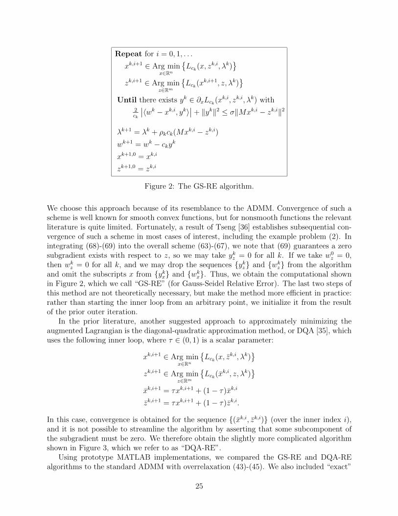
Figure 2: The GS-RE algorithm.

We choose this approach because of its resemblance to the ADMM. Convergence of such ascheme is well known for smooth convex functions, but for nonsmooth functions the relevantliterature is quite limited. Fortunately, a result of Tseng [36] establishes subsequential con-vergence of such a scheme in most cases of interest, including the example problem (2). Inintegrating (68)-(69) into the overall scheme (63)-(67), we note that (69) guarantees a zerosubgradient exists with respect to z, so we may take ykz = 0 for all k. If we take w0

z = 0,then wkz = 0 for all k, and we may drop the sequences {ykz} and {wkz} from the algorithmand omit the subscripts x from {ykx} and {wkx}. Thus, we obtain the computational shownin Figure 2, which we call “GS-RE” (for Gauss-Seidel Relative Error). The last two steps ofthis method are not theoretically necessary, but make the method more efficient in practice:rather than starting the inner loop from an arbitrary point, we initialize it from the resultof the prior outer iteration.

In the prior literature, another suggested approach to approximately minimizing theaugmented Lagrangian is the diagonal-quadratic approximation method, or DQA [35], whichuses the following inner loop, where τ ∈ (0, 1) is a scalar parameter:

xk,i+1 ∈ Arg minx∈Rn

{Lck(x, zk,i, λk)

}zk,i+1 ∈ Arg min

z∈Rm

{Lck(xk,i, z, λk)

}xk,i+1 = τxk,i+1 + (1− τ)xk,i

zk,i+1 = τxk,i+1 + (1− τ)zk,i.

In this case, convergence is obtained for the sequence {(xk,i, zk,i)} (over the inner index i),and it is not possible to streamline the algorithm by asserting that some subcomponent ofthe subgradient must be zero. We therefore obtain the slightly more complicated algorithmshown in Figure 3, which we refer to as “DQA-RE”.

Using prototype MATLAB implementations, we compared the GS-RE and DQA-REalgorithms to the standard ADMM with overrelaxation (43)-(45). We also included “exact”

25

Repeat for i = 0, 1, . . .

xk,i+1 ∈ Arg minx∈Rn

{Lck(x, zk,i, λk)

}zk,i+1 ∈ Arg min

z∈Rm

{Lck(xk,i, z, λk)

}xk,i+1 = τxk,i+1 + (1− τ)xk,i

zk,i+1 = τxk,i+1 + (1− τ)zk,i

Until there exists (ykx, ykz ) ∈ ∂(x,z)Lck(xk,i, zk,i, λk) with

2ck

∣∣∣〈wkx − xk,i, ykx〉+ 〈wkz − zk,i, ykz 〉∣∣∣+ ‖ykx‖2 + ‖ykz‖2 ≤ σ

∥∥Mxk,i − zk,i∥∥2

λk+1 = λk + ρkck(Mxk,i − zk,i)wk+1x = wkx − ckykx

wk+1z = wkz − ckykz

xk+1,0 = xk,i

zk+1,0 = zk,i.

Figure 3: The DQA-RE algorithm.

versions of the Gauss-Seidel and DQA methods in which the respective inner loops of GS-REand DQA-RE are iterated until they obtain a very small augmented Lagrangian subgradient(with norm not exceeding some small fixed parameter δ) or a large iteration limit is reached.We call these methods “GS” and “DQA”, respectively. The exact Gauss-Seidel approachwas described, along with the original proposal for the ADMM, in [17, pages 68-69], whilethe exact DQA method was proposed in [35].

6.2 Computational Tests for the Lasso Problem

We performed tests on two very different problem classes. The first class consisted of sixinstances of the lasso problem (2) derived from standard cancer DNA microarray datasets [8].These instances have very “wide” observation matrices A, with the number of rows p rangingfrom 42 to 102, but the number of columns n ranging from 2000 to 6033.

As mentioned in the introduction, the lasso problem (2) may be reduced to the form (1)by taking

f(x) = 12‖Ax− b‖2 g(z) = ν ‖z‖1 M = I.

The x-minimization step (43) of the ADMM — or equivalently the first minimization in theinner loop of GS-RE or DQA-RE — then reduces to solving a system of linear equationsinvolving the matrix A>A+ cI, namely (in the ADMM case)

xk+1 = (A>A+ cI)−1 (A>b+ czk − λk). (70)

As long as the parameter c remains constant throughout the algorithm, the matrix A>A+ cIneed only be factored once at the outset, and each iteration only involves backsolving the

26

system using this factorization. Furthermore, for “wide” matrices such as those in thedataset of [8], one may use the Sherman-Morrison-Woodbury inversion formula to substitutea factorization of the much smaller matrix I + 1

cAA> for the factorization of A>A+ cI; each

iteration then requires a much faster, lower-dimensional backsolve operation, along with someadditional matrix multiplications and simple vector arithmetic. The z-minimization (44) —or equivalently the second minimization in the inner loop of the GS-RE or DQA-RE —reduces to a very simple componentwise “vector shrinkage” operation. In the ADMM case,this shrinkage operation is

zk+1i = sgn(xk+1

i + 1cλki ) max

{0,∣∣xk+1i + 1

cλki∣∣− ν

c

}i = 1, . . . , n. (71)

Since M = I, the multiplier update (45) is also a very simple componentwise calculation,so the backsolves required to implement the x-minimization dominate the time required foreach ADMM iteration.

Applying the GS-RE and DQA-RE algorithms to the lasso problem results in x- and z-minimizations respectively very similar to (70) and (71), these algorithms’ multiplier updatesare nearly identical to the ADMM, and their inner-loop termination tests require only a fewinner-product calculations. Thus, the x-minimization step also dominates the per-iterationtime for all the algorithms tested. For a more detailed discussion of applying the ADMM tothe lasso problem (2), see for example [6].

Our computational tests used a standard method for normalizing the matrix A, scal-ing each column to have norm 1 and also scaling b to have norm 1; after performing thisnormalization, the problem scaling parameter ν was set to 0.1‖A>b‖∞.

After some experimentation, we settled on the following algorithm parameter settings,which seemed to work well for all the algorithms tested: regarding the penalty parameters,we chose c = 10 for the ADMM and ck ≡ 10 for the other algorithms. For overrelaxation,we chose ρk ≡ ρ = 1.95 for all the algorithms. For the DQA inner loop, we set τ = 0.5.

For all algorithms, the initial Lagrange muliplier estimate λ0 was the zero vector; allprimal variables were also initialized to zero. For all algorithms, the overall terminationcriterion was

dist∞(0, ∂x

[12‖Ax− b‖2 + ν ‖x‖1

]x=xk

)≤ ε, (72)

where dist∞(t, S) = inf {‖t− s‖∞ | s ∈ S }, and ε is a tolerance parameter we set 10−6. Inthe relative-error augmented Lagrangian methods, GS-RE and DQA-RE, we set the param-eter σ to 0.99. For the “exact” versions of these methods, GS and DQA respectively, weterminated the inner loop when

dist∞(0, ∂(x,z)

[Lck(x

k,i, zk,i, λk)])≤ ε

10, (73)

or after 20,000 inner loop iterations, whichever came first. Note that the overall terminationcondition (72) is in practice much stronger than the “relative error” termination conditionsdescribed in [6] (where the term “relative error” is used in a different sense than in this paperand [13]). Empirically, we found that using an “accuracy” of 10−4 with the relative errorconditions of [6] could still result in errors as great as 5% in the objective function, so weused the more stringent and stable condition (72) instead.

Table 1 and Figure 4 show the number of multiplier adjustment steps for each combinationof the six problem instance in the test set of [8] and each of the five algorithms tested; for

27

Table 1: Lasso problems: number of outer iterations / multiplier adjustments

Problem Instance ADMM GS-RE DQA-RE GS DQABrain 814 219 272 277 281Colon 1,889 213 237 237 211Leukemia 1,321 200 218 239 212Lymphoma 1,769 227 253 236 209Prostate 838 213 238 237 210SRBCT 2,244 216 232 254 226

0

500

1000

1500

2000

2500

Brain Colon Leukemia Lymphoma Prostate SRBCT

ADMM

GS-RE

DQA-RE

GS

DQA

Figure 4: Lasso problems: number of outer iterations / multiplier adjustments

the ADMM, the number of multiplier adjustments is simply the total number of iterations,whereas for the other algorithms it is the number of times the outer (over k) loop wasexecuted until the convergence criterion (72) was met.

Generally speaking, the ADMM method requires between 4 and 10 times as many mul-tiplier adjustments as the other algorithms. Note that even with highly approximate mini-mization of the augmented Lagrangian as implied by the choice of σ = 0.99 in the GS-REand DQA-RE methods, their number of multiplier adjustments is far smaller than for theADMM method. Comparing the four non-ADMM methods, there is very little variationin the number of multiplier adjustments, so there does not seem to be much penalty forminimizing the augmented Lagrangian approximately rather than almost exactly; however,there is a penalty in terms of outer iterations for the ADMM’s strategy of updating themultipliers as often as possible, regardless of how little progress may have been made towardminimizing the augmented Lagrangian.

A different picture emerges when we examine total number of inner iterations for each

28

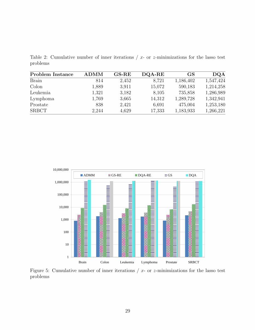
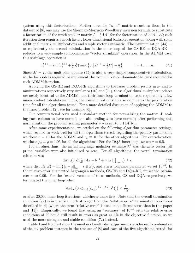
Table 2: Cumulative number of inner iterations / x- or z-minimizations for the lasso testproblems

Problem Instance ADMM GS-RE DQA-RE GS DQABrain 814 2,452 8,721 1,186,402 1,547,424Colon 1,889 3,911 15,072 590,183 1,214,258Leukemia 1,321 3,182 8,105 735,858 1,286,989Lymphoma 1,769 3,665 14,312 1,289,728 1,342,941Prostate 838 2,421 6,691 475,004 1,253,180SRBCT 2,244 4,629 17,333 1,183,933 1,266,221

1

10

100

1,000

10,000

100,000

1,000,000

10,000,000

Brain Colon Leukemia Lymphoma Prostate SRBCT

ADMM GS-RE DQA-RE GS DQA

Figure 5: Cumulative number of inner iterations / x- or z-minimizations for the lasso testproblems

29

0

2,000

4,000

6,000

8,000

10,000

12,000

14,000

16,000

18,000

Brain Colon Leukemia Lymphoma Prostate SRBCT

ADMM

GS-RE

DQA-RE

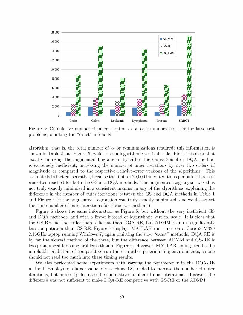
Figure 6: Cumulative number of inner iterations / x- or z-minimizations for the lasso testproblems, omitting the “exact” methods

algorithm, that is, the total number of x- or z-minimizations required; this information isshown in Table 2 and Figure 5, which uses a logarithmic vertical scale. First, it is clear thatexactly minizing the augmented Lagrangian by either the Gauss-Seidel or DQA methodis extremely inefficient, increasing the number of inner iterations by over two orders ofmagnitude as compared to the respective relative-error versions of the algorithms. Thisestimate is in fact conservative, because the limit of 20,000 inner iterations per outer iterationwas often reached for both the GS and DQA methods. The augmented Lagrangian was thusnot truly exactly minimized in a consistent manner in any of the algorithms, explaining thedifference in the number of outer iterations between the GS and DQA methods in Table 1and Figure 4 (if the augmented Lagrangian was truly exactly minimized, one would expectthe same number of outer iterations for these two methods).

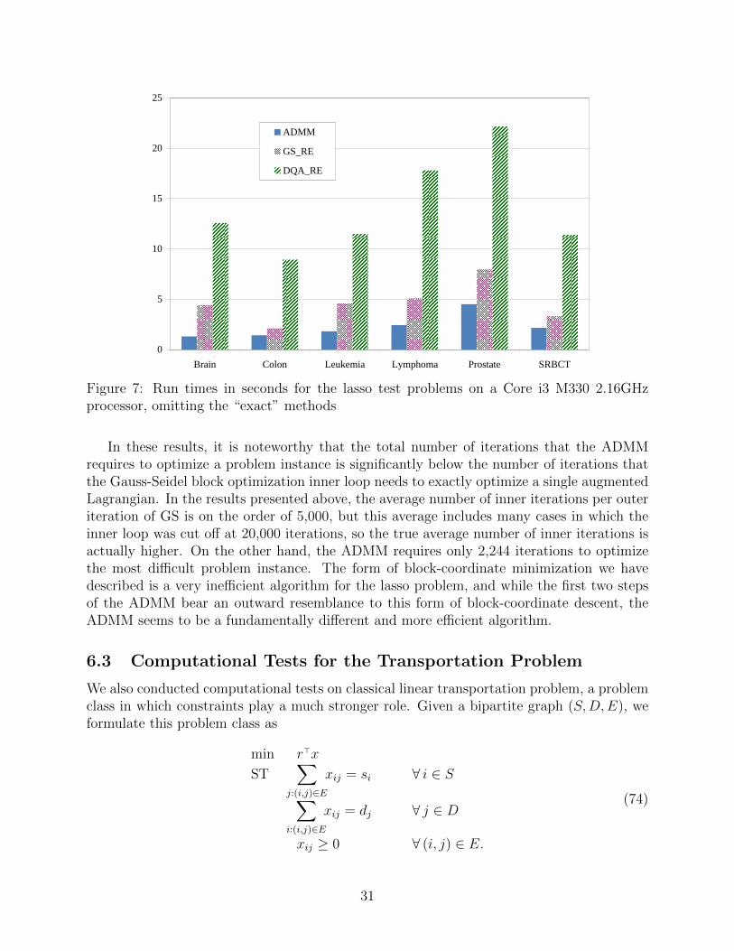
Figure 6 shows the same information as Figure 5, but without the very inefficient GSand DQA methods, and with a linear instead of logarithmic vertical scale. It is clear thatthe GS-RE method is far more efficient than DQA-RE, but ADMM requires significantlyless computation than GS-RE. Figure 7 displays MATLAB run times on a Core i3 M3302.16GHz laptop running Windows 7, again omitting the slow “exact” methods: DQA-RE isby far the slowest method of the three, but the difference between ADMM and GS-RE isless pronounced for some problems than in Figure 6. However, MATLAB timings tend to beunreliable predictors of comparative run times in other programming environments, so oneshould not read too much into these timing results.

We also performed some experiments with varying the parameter τ in the DQA-REmethod. Employing a larger value of τ , such as 0.8, tended to increase the number of outeriterations, but modestly decrease the cumulative number of inner iterations. However, thedifference was not sufficient to make DQA-RE competitive with GS-RE or the ADMM.

30

0

5

10

15

20

25

Brain Colon Leukemia Lymphoma Prostate SRBCT

ADMM

GS_RE

DQA_RE

Figure 7: Run times in seconds for the lasso test problems on a Core i3 M330 2.16GHzprocessor, omitting the “exact” methods

In these results, it is noteworthy that the total number of iterations that the ADMMrequires to optimize a problem instance is significantly below the number of iterations thatthe Gauss-Seidel block optimization inner loop needs to exactly optimize a single augmentedLagrangian. In the results presented above, the average number of inner iterations per outeriteration of GS is on the order of 5,000, but this average includes many cases in which theinner loop was cut off at 20,000 iterations, so the true average number of inner iterations isactually higher. On the other hand, the ADMM requires only 2,244 iterations to optimizethe most difficult problem instance. The form of block-coordinate minimization we havedescribed is a very inefficient algorithm for the lasso problem, and while the first two stepsof the ADMM bear an outward resemblance to this form of block-coordinate descent, theADMM seems to be a fundamentally different and more efficient algorithm.

6.3 Computational Tests for the Transportation Problem

We also conducted computational tests on classical linear transportation problem, a problemclass in which constraints play a much stronger role. Given a bipartite graph (S,D,E), weformulate this problem class as

min r>x

ST∑

j:(i,j)∈E

xij = si ∀ i ∈ S∑i:(i,j)∈E

xij = dj ∀ j ∈ D

xij ≥ 0 ∀ (i, j) ∈ E.

(74)

31

Here, xij is the flow on edge (i, j) ∈ E, si is the supply at source i ∈ S, and dj is thedemand at destination node j ∈ D. Also, x ∈ R|E| is the vector of all the flow variables xij,(i, j) ∈ E, and r ∈ R|E|, whose coefficients are similarly indexed as rij, is the vector of unittranportation costs on the edges.

One way this problem may be formulated in the form (1) or (3) is as follows: let m =n = |E| and define

f(x) =

12r>x, if x ≥ 0 and

∑j:(i,j)∈E

xij = si ∀ i ∈ S

+∞ otherwise

g(z) =

12r>z, if z ≥ 0 and

∑i:(i,j)∈E

zij = dj ∀ j ∈ D

+∞ otherwise.

Again taking M = I, problem (3) is now equivalent to (74). Essentially, the +∞ values inf enforce flow balance at all source nodes and the +∞ values in g enforce flow balance atthe destination nodes. Both f and g include the edge costs and the constraint that flows arenonnegative, and the constraints Mx = z, reducing to x = z, require that the flow into eachedge at its source is equal to the flow out of the edge at its destination.

Applying the ADMM (43)-(45) to this choice of f , g, and M results in a highly paral-lelizable algorithm. The x-minimization (43) reduces to solving the following optimizationproblem independently for each source node i ∈ S:

min 12

∑j: (i,j)∈E

rijxij +∑

j: (i,j)∈E

λijxij + c2

∑j: (i,j)∈E

(xij − zij)2

ST∑

j: (i,j)∈E

xij = si

xij ≥ 0 ∀ j : (i, j) ∈ E.

(75)

This problem is equivalent to projection onto a simplex, and a simple Lagrange multiplieranalysis shows that it may be solved by sorting the breakpoints and then finding a zerocrossing of a monotone piecewise-linear function. With careful use of linear-time median-finding techniques, the sorting operation may be eliminated, and the entire calculation maybe performed in linear time; see for example [28].

The z-minimization (44) reduces to a very similar set of |D| independent minimizations,one for each j ∈ D:

min 12

∑i: (i,j)∈E

rijzij −∑

i: (i,j)∈E

λijzij + c2

∑i: (i,j)∈E

(zij − (ρkx

k+1ij + (1− ρk)zkij)

)2

ST∑

i: (i,j)∈E

zij = dj

zij ≥ 0 ∀ i : (i, j) ∈ E.

(76)

Finally, because M = I, the multiplier update (45) decomposes into |E| independent tasks,one for each (i, j) ∈ E:

λk+1ij = λkij + c

(ρkx

k+1ij + (1− ρk)zkij − zk+1

ij

). (77)

32

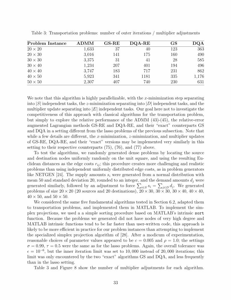
Table 3: Transportation problems: number of outer iterations / multiplier adjustments

Problem Instance ADMM GS-RE DQA-RE GS DQA20× 20 1,633 37 40 123 36320× 30 3,016 141 175 160 49030× 30 3,375 31 41 28 58530× 40 1,234 207 401 194 49640× 40 3,747 183 717 231 86240× 50 5,923 341 1181 335 1,17650× 50 2,307 407 740 230 631

We note that this algorithm is highly parallelizable, with the x-minimization step separatinginto |S| independent tasks, the z-minimization separating into |D| independent tasks, and themultiplier update separating into |E| independent tasks. Our goal here not to investigate thecompetitiveness of this approach with classical algorithms for the transportation problem,but simply to explore the relative performance of the ADMM (43)-(45), the relative-erroraugmented Lagrangian methods GS-RE and DQA-RE, and their “exact” counterparts GSand DQA in a setting different from the lasso problems of the previous subsection. Note thatwhile a few details are different, the x-minimization, z-minimization, and multiplier updatesof GS-RE, DQA-RE, and their “exact” versions may be implemented very similarly in thissetting to their respective counterparts (75), (76), and (77) above.

To test the algorithms, we randomly generated dense problems by locating the sourceand destination nodes uniformly randomly on the unit square, and using the resulting Eu-clidean distances as the edge costs rij; this procedure creates more challenging and realisticproblems than using independent uniformly distributed edge costs, as in problem generatorslike NETGEN [24]. The supply amounts si were generated from a normal distribution withmean 50 and standard deviation 20, rounded to an integer, and the demand amounts dj weregenerated similarly, followed by an adjustment to force

∑i∈S si =

∑j∈D dj. We generated

problems of size 20× 20 (20 sources and 20 destinations), 20× 30, 30× 30, 30× 40, 40× 40,40× 50, and 50× 50.

We considered the same five fundamental algorithms tested in Section 6.2, adapted themto transportation problems, and implemented them in MATLAB. To implement the sim-plex projections, we used a a simple sorting procedure based on MATLAB’s intrinsic sort

function. Because the problems we generated did not have nodes of very high degree andMATLAB intrinsic functions tend to be far faster than user-written code, this approach islikely to be more efficient in practice for our problem instances than attempting to implementthe specialized simplex projection algorithm of [28]. After a modicum of experimentation,reasonable choices of parameter values appeared to be c = 0.005 and ρ = 1.0; the settingsσ = 0.99, τ = 0.5 were the same as for the lasso problems. Again, the overall tolerance wasε = 10−6, but the inner iteration limit was set to 10, 000 instead of 20, 000 iterations; thislimit was only encountered by the two “exact” algorithms GS and DQA, and less frequentlythan in the lasso setting.

Table 3 and Figure 8 show the number of multiplier adjustments for each algorithm.

33

0

1000

2000

3000

4000

5000

6000

7000

20 x 20 20 x 30 30 x 30 30 x 40 40 x 40 40 x 50 50 x 50

ADMM

GS-RE

DQA-RE

GS

DQA

Figure 8: Transportation problems: number of outer iterations / multiplier adjustments

Table 4: Cumulative number of inner iterations / x- or z-minimizations for transportationproblems

Problem Instance ADMM GS-RE DQA-RE GS DQA20× 20 1,633 1,618 5,565 12,731 39,95120× 30 3,016 3,431 11,208 24,919 74,01030× 30 3,375 2,654 7,394 26,139 81,18730× 40 1,234 2,813 7,446 26,241 76,43340× 40 3,747 9,839 19,206 111,500 247,18740× 50 5,923 8,263 27,385 212,774 486,61750× 50 2,307 13,519 41,346 152,260 311,860

Qualitatively, the results are fairly similar to those for lasso problem, although there is morevariability between problem instances and between the the four non-ADMM methods. Asbefore, the ADMM methods requires by far the most outer iterations, but this phenomenonis even more pronounced. For example, for the 20 × 20 problem, the ADMM requires over40 times as many multiplier updates as GS-RE.

Table 4 and Figure 9 show the cumulative inner iteration counts, with Figure 9 employinga logarithmic vertical axis. Figure 10 showns the same data with a linear vertical axis,omitting the two slowest algorithms, GS and DQA. The results are quite similar to those forlasso problems, except that for the three smallest problems ADMM and GS-RE have nearlythe same performance, with GS-RE being faster for one problem. Finally, Figure 11 showscorresponding MATLAB run times on a Xeon X5472 3.00 GHz processor running UbuntuLinux 10.04. These run times closely track the inner iteration counts of Figure 10.

34

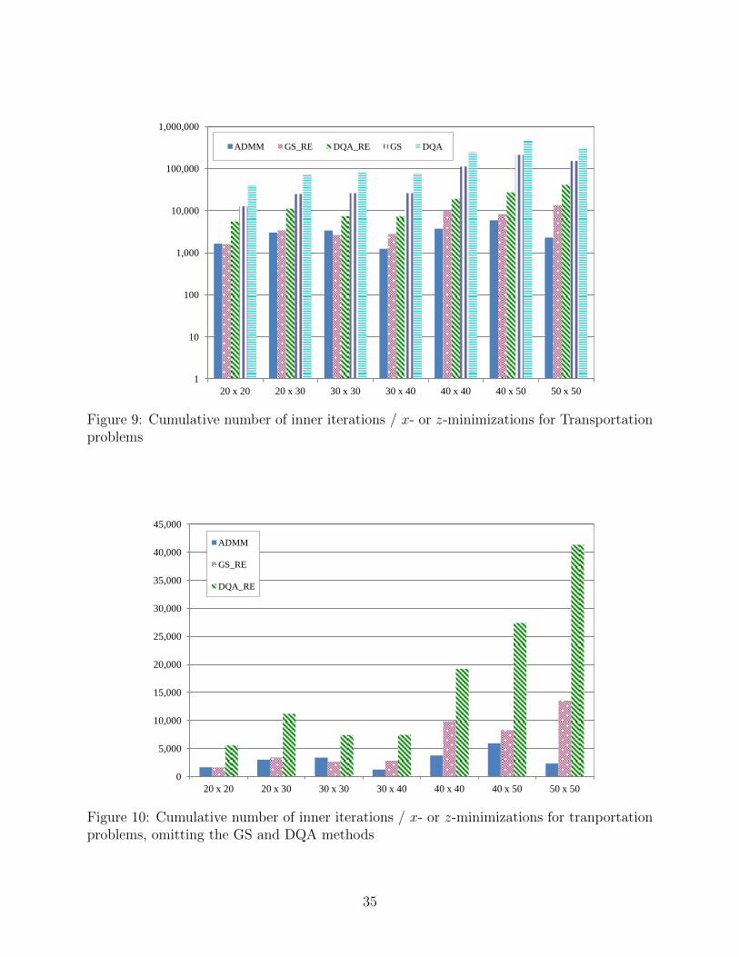
1

10

100

1,000

10,000

100,000

1,000,000

20 x 20 20 x 30 30 x 30 30 x 40 40 x 40 40 x 50 50 x 50

ADMM GS_RE DQA_RE GS DQA

Figure 9: Cumulative number of inner iterations / x- or z-minimizations for Transportationproblems

0

5,000

10,000

15,000

20,000

25,000

30,000

35,000

40,000

45,000

20 x 20 20 x 30 30 x 30 30 x 40 40 x 40 40 x 50 50 x 50

ADMM

GS_RE

DQA_RE

Figure 10: Cumulative number of inner iterations / x- or z-minimizations for tranportationproblems, omitting the GS and DQA methods

35

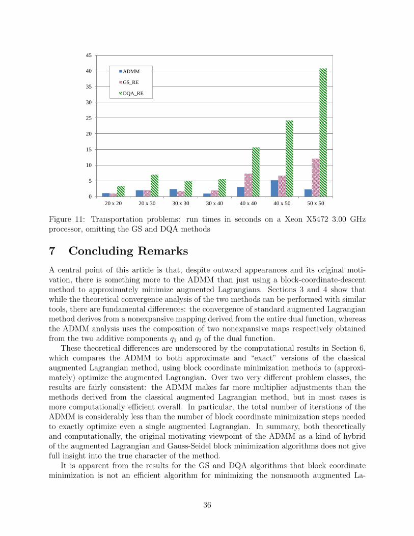
0

5

10

15

20

25

30

35

40

45

20 x 20 20 x 30 30 x 30 30 x 40 40 x 40 40 x 50 50 x 50

ADMM

GS_RE

DQA_RE

Figure 11: Transportation problems: run times in seconds on a Xeon X5472 3.00 GHzprocessor, omitting the GS and DQA methods

7 Concluding Remarks

A central point of this article is that, despite outward appearances and its original moti-vation, there is something more to the ADMM than just using a block-coordinate-descentmethod to approximately minimize augmented Lagrangians. Sections 3 and 4 show thatwhile the theoretical convergence analysis of the two methods can be performed with similartools, there are fundamental differences: the convergence of standard augmented Lagrangianmethod derives from a nonexpansive mapping derived from the entire dual function, whereasthe ADMM analysis uses the composition of two nonexpansive maps respectively obtainedfrom the two additive components q1 and q2 of the dual function.

These theoretical differences are underscored by the computational results in Section 6,which compares the ADMM to both approximate and “exact” versions of the classicalaugmented Lagrangian method, using block coordinate minimization methods to (approxi-mately) optimize the augmented Lagrangian. Over two very different problem classes, theresults are fairly consistent: the ADMM makes far more multiplier adjustments than themethods derived from the classical augmented Lagrangian method, but in most cases ismore computationally efficient overall. In particular, the total number of iterations of theADMM is considerably less than the number of block coordinate minimization steps neededto exactly optimize even a single augmented Lagrangian. In summary, both theoreticallyand computationally, the original motivating viewpoint of the ADMM as a kind of hybridof the augmented Lagrangian and Gauss-Seidel block minimization algorithms does not givefull insight into the true character of the method.

It is apparent from the results for the GS and DQA algorithms that block coordinateminimization is not an efficient algorithm for minimizing the nonsmooth augmented La-

36

grangian functions arising in either of the application classes discussed in Section 6, yet thisphenomenon does not seem to affect the performance of the ADMM. In general, the ADMMseems a superior algorithm to approximate minimization of augmented Lagrangians by blockcoordinate approaches; this conclusion was somewhat unexpected, in that the ADMM has areputation for fairly slow convergence, especially in the “tail”, whereas classical augmentedLagrangian method are generally considered competitive or near-competitive methods, andform the basis for a number of state-of-the-art nonlinear optimization codes. However, theresults here do not necessarily establish the superiority of the ADMM to classical augmentedLagrangian methods using more sophisticated methods to optimize the subproblems.

Acknowledgments

This material is based in part upon work supported by the National Science Foundationunder Grant CCF-1115638. This material was presented in abridged form as a plenarypresentation at the INFORMS Computing Society Conference in Santa Fe, NM in January2013. It is also intended as a more theoretically oriented companion to [6].

References

[1] N. S. Aybat and G. Iyengar. An alternating direction method with increasing penaltyfor stable principal component pursuit. Computational Optimization and Applications,61(3):632–668, 2015.

[2] H. H. Bauschke and P. L. Combettes. Convex Analysis and Monotone Operator Theoryin Hilbert Spaces. Springer, New York, 2011.

[3] D. P. Bertsekas. Convex Analysis and Optimization. Athena Scientific, Belmont, MA,2003. With A. Nedic and A. E. Ozdaglar.

[4] D. P. Bertsekas. Convex Optimization Algorithms. Athena Scientific, 2015.

[5] D. P. Bertsekas and J. N. Tsitsiklis. Parallel and Distributed Computation: NumericalMethods. Prentice Hall, 1989.

[6] S. Boyd, N. Parikh, E. Chu, B. Peleato, and J. Eckstein. Distributed optimization andstatistical learning via the alternating direction method of multipliers. Foundations andTrends in Machine Learning, 3(1):1–122, 2011.

[7] C. Chen, B. He, Y. Ye, and X. Yuan. The direct extension of ADMM for multi-blockconvex minimization problems is not necessarily convergent. Preprint 4059, Optimiza-tion Online, 2013.

[8] M. Dettling and P. Buhlmann. Finding predictive gene groups from microarray data.Journal of Multivariate Analysis, 90(1):106–131, 2004.

[9] J. Eckstein. Splitting methods for monotone operators with applications to parallel op-timization. PhD thesis, MIT, 1989.

37

[10] J. Eckstein. A practical general approximation criterion for methods of multipliers basedon Bregman distances. Mathematical Programming., 96(1):61–86, 2003.

[11] J. Eckstein and D. P. Bertsekas. On the Douglas-Rachford splitting method and theproximal point algorithm for maximal monotone operators. Mathematical Programming,55:293–318, 1992.

[12] J. Eckstein and M. C. Ferris. Operator-splitting methods for monotone affine varia-tional inequalities, with a parallel application to optimal control. INFORMS Journalon Computing, 10(2):218–235, 1998.

[13] J. Eckstein and P. J. S. Silva. A practical relative error criterion for augmented La-grangians. Mathematical Programming, 141(1-2):319–348, 2013.

[14] J. Eckstein and B. F. Svaiter. General projective splitting methods for sums of maximalmonotone operators. SIAM Journal on Control and Optimization, 48:787–811, 2009.

[15] M. Fortin and R. Glowinski. On decomposition-coordination methods using an aug-mented Lagrangian. In M. Fortin and R. Glowinski, editors, Augmented LagrangianMethods: Applications to the Solution of Boundary-Value Problems, pages 97–146.North-Holland: Amsterdam, 1983.

[16] D. Gabay. Applications of the method of multipliers to variational inequalities. InM. Fortin and R. Glowinski, editors, Augmented Lagrangian Methods: Applications tothe Solution of Boundary-Value Problems, pages 299–331. North-Holland: Amsterdam,1983.

[17] R. Glowinski and A. Marroco. Sur l’approximation, par elements finis d’ordre un,et la resolution, par penalisation-dualite, d’une classe de problems de Dirichlet nonlineares. Revue Francaise d’Automatique, Informatique, et Recherche Operationelle,9:41–76, 1975.

[18] B. He, M. Tao, and X. Yuan. Alternating direction method with Gaussian back substi-tution for separable convex programming. SIAM J. Optim., 22(2):313–340, 2012.

[19] B. He, M. Tao, and X. Yuan. Convergence rate and iteration complexity on the al-ternating direction method of multipliers with a substitution procedure for separableconvex programming. Preprint 3611, Optimization Online, 2012.

[20] B.-S. He. Parallel splitting augmented Lagrangian methods for monotone structuredvariational inequalities. Computational Optimization and Applications, 42(2):195–212,2009.

[21] B.-S. He, Z. Peng, and X.-F. Wang. Proximal alternating direction-based contractionmethods for separable linearly constrained convex optimization. Frontiers of Mathe-matics in China, 6(1):79–114, 2011.

38

[22] B.-S. He, H. Yang, and S.-L. Wang. Alternating direction method with self-adaptivepenalty parameters for monotone variational inequalities. Journal of Optimization The-ory and Applications, 106(2):337–356, 2000.

[23] M. Hong and Z.-Q. Luo. On the linear convergence of the alternating direction methodof multipliers. Preprint 1208.3922, arXiv, 2012.

[24] D. Klingman, A. Napier, and J. Stutz. NETGEN: A program for generating large-scale capacitated assignment, transportation, and minimum cost flow network problems.Management Science, 20(5):814–821, 1974.

[25] M. A. Krasnosel’skiı. Two remarks on the method of successive approximations. UspekhiMatematicheskikh Nauk, 10(1):123–127, 1955.

[26] J. Lawrence and J. E. Spingarn. On fixed points of non-expansive piecewise isometricmappings. Proceedings of the London Mathematical Society, 3(3):605, 1987.

[27] P. L. Lions and B. Mercier. Splitting algorithms for the sum of two nonlinear operators.SIAM Journal on Numerical Analysis, 16:964–979, 1979.

[28] N. Maculan and G. G. de Paula, Jr. A linear-time median-finding algorithm for pro-jecting a vector on the simplex of Rn. Operations Research Letters, 8(4):219–222, 1989.

[29] G. J. Minty. Monotone (nonlinear) operators in Hilbert space. Duke MathematicalJournal, 29:341–346, 1962.

[30] R. T. Rockafellar. Convex Analysis. Princeton University Press, 1970.

[31] R. T. Rockafellar. Conjugate Duality and Optimization. SIAM, Philadelphia, 1974.

[32] R. T. Rockafellar. Augmented Lagrangians and applications of the proximal pointalgorithm in convex programming. Mathematics of Operations Research, 1(2):97–116,1976.

[33] R. T. Rockafellar. Monotone operators and the proximal point algorithm. SIAM Journalon Control and Optimization, 14(5):877–898, 1976.

[34] R. T. Rockafellar and R. J.-B. Wets. Scenarios and policy aggregation in optimizationunder uncertainty. Mathematics of Operations Research, 16(1):119–147, 1991.

[35] A. Ruszczynski. On convergence of an augmented Lagrangian decomposition methodfor sparse convex optimization. Mathematics of Operations Research, 20(3):634–656,1995.

[36] P. Tseng. Convergence of a block coordinate descent method for nondifferentiable min-imization. Journal of Optimization Theory and Applications, 109(3):475–494, 2001.

39