Linear models for data science

Linear models for data science

Brad Klingenberg, Director of Styling Algorithms at Stitch [email protected] Insight Data Science, Oct 2015

A brief introduction

Linear models in data science

Goal: give a basic overview of linear modeling and some of its extensions

Linear models in data science

Goal: give a basic overview of linear modeling and some of its extensions

Secret goal: convince you to study linear models and to try simple things first

Linear regression? Really?

Wait... regression? That’s so 20th century!



What about deep learning? What about AI? What about Big Data™?




There are a lot of exciting new tools. But in many problems simple models can take you a long way.




There are a lot of exciting new tools. But in many problems simple models can take you a long way.

Regression is the workhorse of applied statistics

Occam was right!

Simple models have many virtues

Occam was right!


In industry

● Interpretability○ for the developer and the user

● Clear and confident understanding of what the model does● Communication to business partners

Occam was right!


In industry

● Interpretability○ for the developer and the user

● Clear and confident understanding of what the model does● Communication to business partners

As a data scientist

● Enables iteration: clarity on how to extend and improve● Computationally tractable● Often close to optimal in large or sparse problems

An excellent reference

Figures and examples liberally stolen from

[ESL]

Part I: Linear regression

The basic model

We observe N numbers Y = (y_1, …, y_N) from a model

How can we predict Y from X?

The basic model

response global intercept feature j of observation i

coefficient for feature j

noise termnumber of features

noise level

independence assumption

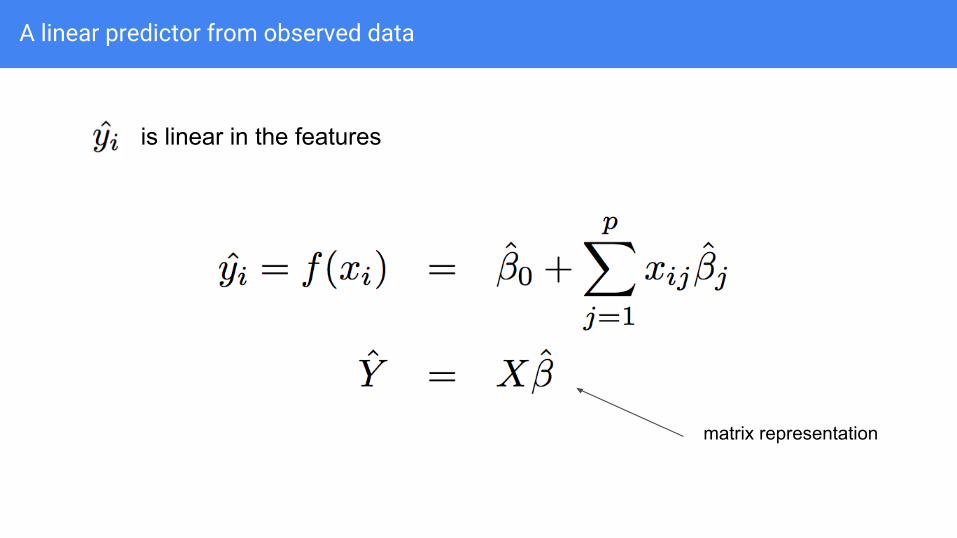
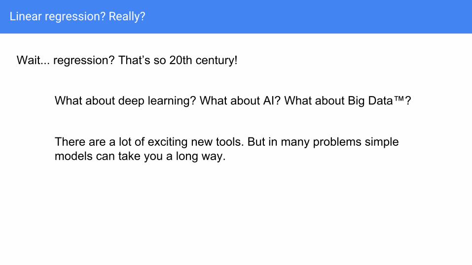
A linear predictor from observed data

matrix representation

is linear in the features

X: the data matrix

Rows are observations

N rows

X: the data matrix

Columns are features p columns

also called

● predictors● covariates● signals

Choosing β

Minimize a loss function to find the β giving the “best fit”

Then

Choosing β

Minimize a loss function to find the β giving the “best fit”

[ESL]

An analytical solution: univariate case

With squared-error loss the solution has a closed-form

An analytical solution: univariate case

“Regression to the mean”

sample correlation distance of predictor from its average

adjustment for scale of variables

A general analytical solution


A general analytical solution


“Hat matrix”

The hat matrix

The hat matrix

X^TX

= X^TX ≈ Σ

● must not be singular or too close to singular (collinearity)

● This assumes you have more observations that features (n > p)

● Uses information about relationships between features

● i is not inverted in practice (better numerical strategies like a QR decomposition are used)

● (optional): Connections to degrees of freedom and prediction error

The hat matrix

Linear regression as projection

data

prediction

span of features

[ESL]

Inference

The linearity of the estimator makes inference easy

Inference

The linearity of the estimator makes inference easy

So that

unbiased known sample covariance

usually have to estimate noise level

Linear hypotheses

Inference is particularly easy for linear combinations of coefficients

scalar

Linear hypotheses

Inference is particularly easy for linear combinations of coefficients

scalarIndividual coefficients

Differences

Inference for single parameters

We can then test for the presence of a single variable

caution! this tests a single variablebut correlation with other variables can make it confusing

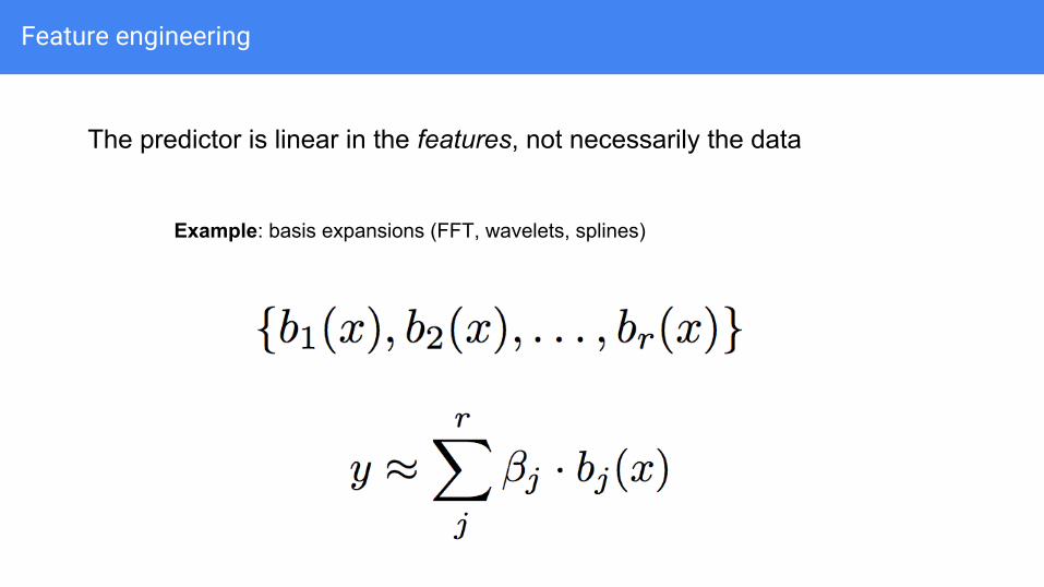
Feature engineering

The predictor is linear in the features, not necessarily the data

Example: simple transformations

Feature engineering

Example: dummy variables


Feature engineering

Example: basis expansions (FFT, wavelets, splines)


Feature engineering

Example: interactions


Why squared error loss?

Why use squared error loss

instead of something else?

or

Why squared error loss?

Why use squared error loss?

● Math on quadratic functions is easy (nice geometry and closed-form solution)● Estimator is unbiased● Maximum likelihood● Gauss-Markov● Historical precedent

Maximum likelihood

Maximum likelihood is a general estimation strategy

Likelihood function

Log-likelihood

MLE

joint density

[wikipedia]

Maximum likelihood

Example: 42 out 100 heads from a fair coin true value

samplemaximum

Why least squares?

For linear regression, the likelihood involves the density of the multivariate normal

After taking the log and simplifying we arrive at (something proportional to) squared error loss

[wikipedia]

MLE for linear regression

There are many theoretical reasons for using the MLE

● The estimator is consistent (will converge to the true parameter in probability)

● The asymptotic distribution is normal, making inference easy if you have enough data

● The estimator is efficient: the asymptotic variance is known and achieves the Cramer-Rao theoretical lower bound

But are we relying too much on the assumption that the errors are normal?

The Gauss-Markov theorem

Suppose that

(no assumption of normality)Then consider all unbiased, linear estimators such that for some matrix W

Gauss-Markov: linear regression has the lowest MSE for any β. (“BLUE”: best linear unbiased estimator)

[wikipedia]

Why not to use squared error loss

Squared error loss is sensitivity to outliers. More robust alternatives: absolute loss, Huber loss

[ESL]

Part II: Generalized linear models

Binary data

The linear model no longer makes sense as a generative model for binary data

… but

However, it can still be very useful as a predictive model.

Generalized linear models

To model binary outcomes: model the mean of the response given the data

link function

Example link functions

● Linear regression

● Logistic regression

● Poisson regression

For more reading: The choice of the link function is related to the natural parameter of an exponential family

Logistic regression

[Agresti]

Sample data: empirical proportions as a function of the predictor

Choosing β

Choosing β: maximum likelihood!

Key property: problem is convex! Easy to solve with Newton-Raphson or any convex solver

Optimality properties of the MLE still apply.

Convex functions

[Boyd]

Part III: Regularization

Regularization

Regularization is a strategy for introducing bias.

This is usually done in service of

● incorporating prior information

● avoiding overfitting

● improving predictions


Ridge regression

Ridge regression

Add a penalty to the least-squares loss function

This will “shrink” the coefficients towards zero

Ridge regression


penalty weight; tuning parameter

An old idea: Tikhonov regularization

Ridge regression


Still linear, but changes the hat matrix by adding a “ridge” to the sample covariance matrix

closer to diagonal - puts less faith in sample correlations

Correlated features

Ridge regression will tend to spread weight across correlated features

Toy example: two perfectly correlated features (and no noise)

Correlated features

To minimize L2 norm among all convex combinations of x1 and x2

the solution is to put equal weight on each feature

Ridge regression

Don’t underestimate ridge regression!

Good advice in life:


Bias and variance

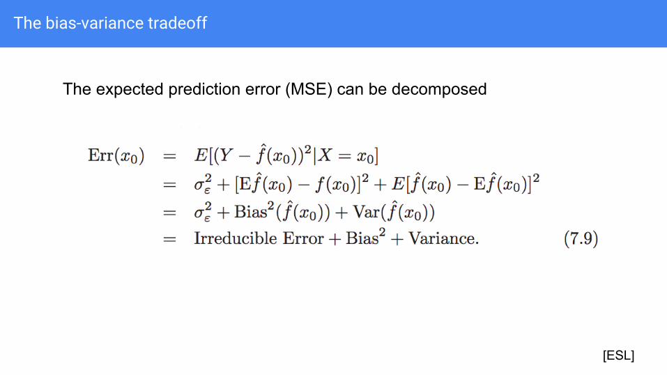
The bias-variance tradeoff

The expected prediction error (MSE) can be decomposed

[ESL]

The bias-variance tradeoff

[ESL]


James-Stein

Historical connection: The James-Stein estimator

Shrinkage is a powerful idea found in many statistical applications.

In the 1950’s Charles Stein shocked the statistical world with (a version of) the following result.

Let μ be a fixed, arbitrary p-vector and suppose we observe one observation of y

[Efron]

The MLE for μ is just the observed vector

The James-Stein estimator

[Efron]

The James-Stein estimator pulls the observation toward the origin

shrinkage

The James-Stein estimator

[Efron]

Theorem: For p >=3, the JS estimator dominates the MLE for any μ!

Shrinking is always better.

The amount of shrinkage depends on all elements of y, even though the elements of μ don’t necessarily have anything to do with each other and the noise is independent!

An empirical Bayes interpretation

[Efron]

Put a prior on μ

Then the posterior mean is

This is JS with the unbiased estimate

James-Stein

The surprise is that JS is always better, even without the prior assumption

[Efron]


LASSO

LASSO

Superficially similar to ridge regression, but with a different penalty

Called “L1” regularization

L1 regularization

Why L1?

Sparsity!

For some choices of the penalty parameter L1 regularization will cause many coefficients to be exactly zero.

L1 regularization

The LASSO can be defined as a closely related to the constrained optimization problem

which is equivalent* to minimizing (Lagrange)

for some λ depending on c.

LASSO: geometric intuition

[ESL]

L1 regularization

Bayesian interpretation

Both ridge regression and the LASSO have a simple Bayesian interpretation

Maximum a posteriori (MAP)

Up to some constants

model likelihood prior likelihood

Maximum a posteriori (MAP)

Ridge regression is the MAP estimator (posterior mode) for the model

For L1: Laplace distribution instead of normal

Compressed sensing

L1 regularization has deeper optimality properties.

Slide from Olga V. Holtz: http://www.eecs.berkeley.edu/~oholtz/Talks/CS.pdf

http://www.eecs.berkeley.edu/~oholtz/Talks/CS.pdf

Basis pursuit



Equivalence of problems



Compressed sensing

Many random matrices have similar incoherence properties - in those cases the LASSO gets it exactly right with only mild assumptions

Near-ideal model selection by L1 minimization [Candes et al, 2007]

Betting on sparsity

[ESL]

When you have many more predictors than observations it can pay to bet on sparsity


Elastic-net

Elastic-net

The Elastic-net blends the L1 and L2 norms with a convex combination

It enjoys some properties of both L1 and L2 regularization

● estimated coefficients can be sparse● coefficients of correlated features are pulled together● still nice and convex

tuning parameters

Elastic-net

The Elastic-net blends the L1 and L2 norms with a convex combination

[ESL]


Grouped LASSO

Grouped LASSO

Regularize for sparsity over groups of coefficients

[ESL]

Grouped LASSO

Regularize for sparsity over groups of coefficients - tends to set entire groups of coefficients to zero. “LASSO for groups”

design matrix for group l

coefficient vector for group l

L2 norm not squared[ESL]


Choosing regularization parameters


The practitioner must choose the penalty. How can you actually do this?

One simple approach is cross-validation

[ESL]


Choosing an optimal regularization parameter from a cross-validation curve

[ESL]

model complexity


Choosing an optimal regularization parameter from a cross-validation curve

Warning: this can easily get out of hand with a grid search over multiple tuning parameters!

[ESL]

Part IV: Extensions

Part IV: Extensions

Weights

Adding weights

It is easy to add weights to most linear models

weights

Adding weights

This is related to generalized least squares for more general error models

Leads to

Part IV: Extensions

Constraints

Non-negative least squares

Non-negative coefficients - still convex

Structured constraints: Isotonic regression

Monotonicity in coefficients

[wikipedia]

for i >= j

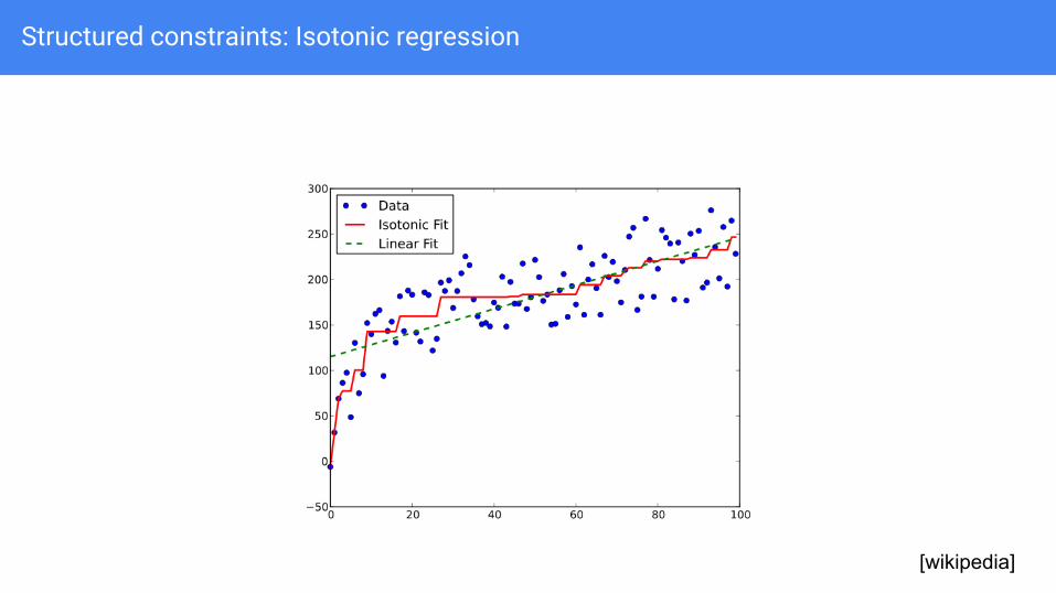
Structured constraints: Isotonic regression

[wikipedia]

Part IV: Extensions

Generalized additive models


Move from linear combinations


Sum of functions of your features


[ESL]


Extremely flexible algorithm for a wide class of smoothers: splines, kernels, local regressions...

[ESL]

Part IV: Extensions

Support vector machines


[ESL]

Maximum margin classification


Can be recast a regularized regression problem

[ESL]


The hinge loss function

[ESL]

SVM kernels

Like any regression, SVM can be used with a basis expansion of features

[ESL]

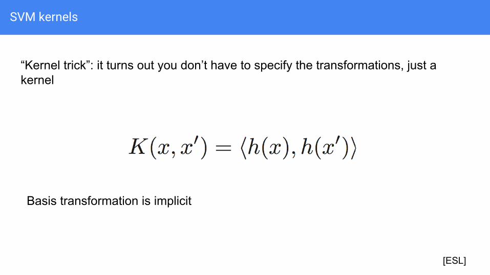
SVM kernels

“Kernel trick”: it turns out you don’t have to specify the transformations, just a kernel

[ESL]

Basis transformation is implicit

SVM kernels

Popular kernels for adding non-linearity

Part IV: Extensions

Mixed effects

Mixed effects models

Add an extra term to the linear model

Mixed effects models

Add an extra term to the model

another design matrix

random vector

independent noise

Motivating example: dummy variables

Indicator variables for individuals in a logistic model

Priors:

Motivating example: dummy variables

Indicator variables for individuals in a logistic model

Priors:

deltas from baseline

L2 regularization

MAP estimation leads to minimizing

How to choose the prior variances?

Selecting variances is equivalent to choosing a regularization parameter. Some reasonable choices:

● Go full Bayes: put priors on the variances and sample

● Use a cross-validation and a grid search

● Empirical Bayes: estimate the variances from the data

Empirical Bayes (REML): you integrate out random effects and do maximum likelihood for variances. Hard but automatic!

Interactions

More ambitious: add an interaction

But, what about small sample sizes?

Interactions

More ambitious: add an interaction

But, what about small sample sizes?

delta from baseline and main effects

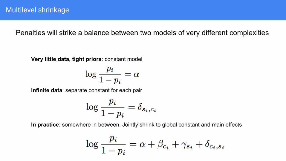
Multilevel shrinkage

Penalties will strike a balance between two models of very different complexities

Very little data, tight priors: constant model

Infinite data: separate constant for each pair

In practice: somewhere in between. Jointly shrink to global constant and main effects

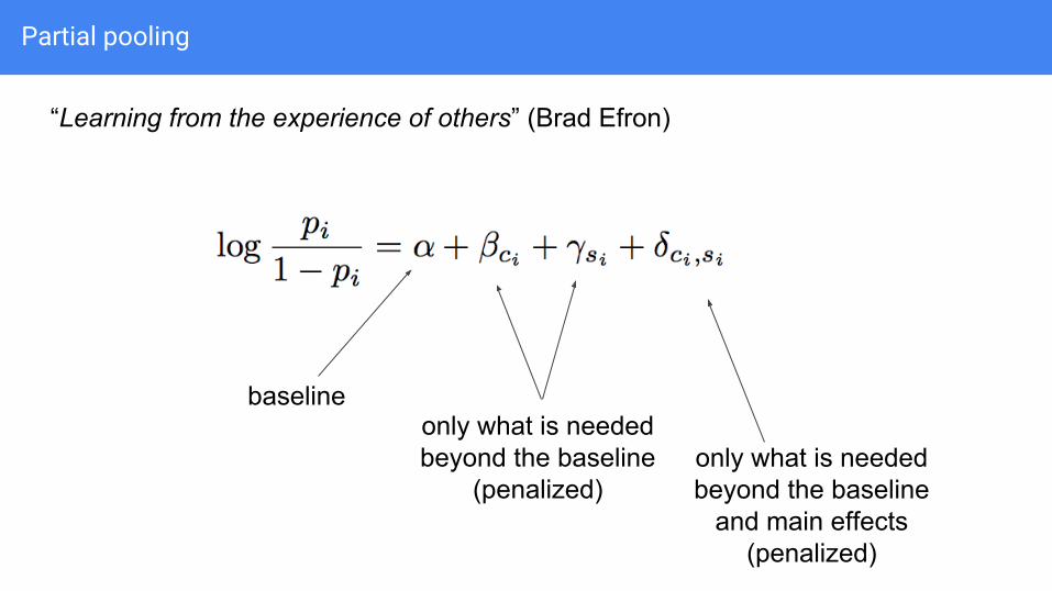
Partial pooling

“Learning from the experience of others” (Brad Efron)

only what is needed beyond the baseline

(penalized)only what is needed beyond the baseline

and main effects(penalized)

baseline

Mixed effects

Model is very general - extends to random slopes and more interesting covariance structures

another design matrix

random vector

independent noise

Bayesian perspective on multilevel models (great reference)

Some excellent references

[ESL] [Agresti] [Boyd] [Efron]

Thanks!

Questions?

[email protected]

Linear models for data science

Data & Analytics

Transcript of Linear models for data science