1

LinearmodelsandlinearmixedeffectsmodelsinR:Tutorial11BodoWinter

UniversityofCalifornia,Merced,CognitiveandInformationSciences

Lastupdated:01/19/2013;08/13/2013;10/01/13;24/03/14;24/04/14;18/07/14;11/03/16

Linearmodelsandlinearmixedmodelsareanimpressivelypowerfulandflexibletool for understanding theworld. This tutorial is the first of two tutorials thatintroduceyoutothesemodels.Thetutorialsaredecidedlyconceptualandomitalotofthemoreinvolvedmathematicalstuff.Thefocusisonunderstandingwhatthesemodels aredoing…and thenwe’ll spendmostof the timeapplying thisunderstanding.Theideaistobootstrapyourknowledgeasquicklyaspossiblesothatyoucanstartwithyourownanalysesandthenturntomoretechnicaltextsifneeded.You’llneedabout1hourtocompletethistutorial(maybeabitmore).So,whatdoes the linearmodeldo?Assumeyouknewnothingaboutmalesandfemales,andyouwereinterestedinwhetherthevoicepitchofmalesandfemalesdiffers,andifso,byhowmuch.Soyoutakeabunchofmalesandabunchoffemales,andaskthemtosayasingleword,say“mama”,andyoumeasuretherespectivevoicepitches.Yourdatamightlooksomethinglikethis:

1For updates and other tutorials, check my webpage www.bodowinter.com. If you have anysuggestions,pleasewritemeanemail:bodo@bodowinter.comPleaseciteas:Winter,B.(2013).LinearmodelsandlinearmixedeffectsmodelsinRwithlinguisticapplications.arXiv:1308.5499.[http://arxiv.org/pdf/1308.5499.pdf]

2

Subject Sex Voice.Pitch 1 female 233Hz 2 female 204Hz 3 female 242Hz 4 male 130Hz 5 male 112Hz 6 male 142Hz“Hz”(Hertz)isameasureofpitchwherehighervaluesmeanhigherpitch.You might look at this table and say that it’s quite obvious that females havehighervoicepitchthanmales.Afterall, thefemalevaluesseemtobeabout100Hzabovethemaleones.But,infact,itcouldbethecasethatfemalesandmaleshavethesamepitch,andyouwerejustunluckyandhappenedtochoosesomeexceptionallyhigh-pitchedfemalesandsomeexceptionallylow-pitchedmales.Intuitively,thepatterninthetableseemsprettystraightforward,butwemightwantamorepreciseestimateofthedifferencebetweenmalesandfemales,andwemightalsowantanestimateabouthowlikely(orunlikely)thatdifferenceinvoicepitchcouldhavearisenjustbecauseofdrawinganunluckysample.Thisiswherethelinearmodelcomesin.Inthiscase,itstaskistogiveyousomevalues about voice pitch for males and females… as well as some probabilityvalueastohowlikelythosevaluesare.The basic idea is to express your relationship of interest (in this case, the onebetweensexandvoicepitch)asasimpleformula…suchasthisone: pitch~sexThisreads “pitchpredictedbysex”or “pitchasa functionofsex”.Somepeoplecall the thingon the left the “dependentvariable” (the thingyoumeasure)andthe thing on the right the “independent variable”. Others call the thing on therightthe“explanatoryvariable”(thissoundstoocausaltome)orthe“predictor”.I’llcallit“fixedeffect”,andthisterminologywillmakesenselateronintutorial2.Now, theworld isn’t perfect. Things aren’t quite as deterministic as the aboveformulasuggests.Pitchisnotcompletelydeterminedbysex,butalsobyabunchofdifferentfactorssuchaslanguage,dialect,personality,ageandwhatnot.Evenifwemeasuredallofthesefactors,therewouldstillbeotherfactorsinfluencingpitchthatwecannotcontrolfor.Perhaps,asubjectinyourdatahadahangoveronthemorningoftherecording(causingthevoicetobelowerthanusual),orthesubject was justmore nervous on that particular day (causing the voice to behigher).Wecannevermeasureandcontrolallofthesethings.Theworldisfullof

3

stuffthatisoutsidethepurviewofourlittleexperiment.Hence,let’supdateourformulatocapturetheexistenceofthese“random”factors. pitch~sex+εThis“ε”(read“epsilon”)isanerrorterm.Itstandsforallofthethingsthataffectpitch that are not sex, all of the stuff that – from the perspective of ourexperiment–israndomoruncontrollable.Theformulaaboveisaschematicdepictionofthelinearmodelthatwe’regoingto build. Note that the part of the formula on the right-hand side conceptuallydividestheworld intostuff thatyoucanunderstand(the“fixedeffect”sex)andstuffthatyoucan’tunderstand(therandompart“ε”).Youcouldcalltheformerthe“structural”or“systematic”partofyourmodelandthelatterthe“random”or“probabilistic”partofthemodel.

Hands-onexercise:Let’sstart!O.k., let’smovetoR, thestatisticalprogrammingenvironmentthatwe’lluse forthe restof this tutorial2. Let’s create thedataset thatwe’lluse forouranalysis.Typein: pitch = c(233,204,242,130,112,142)

sex = c(rep("female",3),rep("male",3)) Thefirstlineconcatenatesour6datapointsfromaboveandsavesitinanobjectthatwenamedpitch. The second line repeats theword “female”3 timesandthen theword“male”3 times…andconcatenates these6words intoanobjectthatwenamedsex.Forabetteroverview,let’scombinethesetwoobjectsintoadataframe: my.df = data.frame(sex,pitch) Nowwehave a data frameobject thatwenamedmy.df, and if you type that,you’llseethis:

2You don’t have R? Don’t worry, it’s free and works on all platforms. You can get it here:http://www.r-project.org/Youmightwant to readaquick intro toRbeforeyouproceed–butevenifyoudon’t,you’llbeabletofolloweverything.Justtypeineverythingyouseeindarkblue.

4

O.k., nowwe’ll proceedwith the linearmodel.We take our formula above andfeed it into thelm() function…except thatweomit the “ε” term,because thelinearmodelfunctiondoesn’tneedyoutospecifythis. xmdl = lm(pitch ~ sex, my.df) Wemodeledpitchasafunctionofsex,takenfromthedataframemy.df…andwesavedthismodelintoanobjectthatwenamedxmdl.Toseewhatthelinearmodeldid,wehaveto“summarize”thisobjectusingthefunctionsummary(): summary(xmdl) Ifyoudothis,youshouldseethis:

Lots of stuff here. First, you’re being reminded of themodel formula that youentered.Then, themodelgivesyoutheresiduals(whatthis iswillbediscussedlater),andthecoefficientsof the fixedeffects(again,explanations follow…bearwithmeforamoment).Then,theoutputprintssomeoverallresultsofthemodelthatyouconstructed.

5

Wehavetoworkthroughthisoutput.Let’sstartwith“MultipleR-Squared”.Thisrefers to the statistic R2 which is a measure of “variance explained” or if youpreferlesscausallanguage,itisameasureof“varianceaccountedfor”.R2valuesrangefrom0to1.OurR2is0.921,whichisquitehigh…youcaninterpretthisasshowingthat92.1%ofthestuffthat’shappeninginourdatasetis“explained”byourmodel. Inthiscase,becausewehaveonlyonethinginourmodeldoingtheexplaining(thefixedeffect“sex”),theR2reflectshowmuchvarianceinourdataisaccountedforbydifferencesbetweenmalesandfemales.Ingeneral,youwantR2valuestobehigh,butwhatisconsideredahighR2valuedependsonyourfieldandonyourphenomenonofstudy.Ifthesystemyoustudyis verydeterministic,R2 values can approach1.But inmost of biology and thesocialsciences,wherewestudycomplexormessysystemsthatareaffectedbyawhole bunch of different phenomena, we frequently deal with much lower R2values.The“AdjustedR-squared”valueisaslightlydifferentR2valuethatnotonlylooksathowmuchvarianceis“explained”,butalsoathowmanyfixedeffectsyouusedtodotheexplaining.So,inthecaseofourmodelabove,thetwovaluesarequitesimilar toeachother,but insomecasestheadjustedR2adjcanbemuch lower ifyouhavealotoffixedeffects(say,youalsousedage,psychologicaltraits,dialectetc.topredictpitch).SomuchforR2.Nextlinedownyouseethethingthateverybodyiscrazyfor:Yourstatistical test of “significance”. If you’ve already done research, your eyeswillprobablyimmediatelyjumptothep-value,whichinmanyfieldsisyourticketforpublishing yourwork. There’s a little bit of an obsessionwith p-values … andeven though they are regarded as so important, they are quite oftenmisunderstood!Sowhatexactlydoesthep-valuemeanhere?One way to phrase it is to say that assuming yourmodel is doing nothing, theprobabilityofyourdataisrelativelylow(becausethep-valueissmallinthiscase).Technicallyspeaking,thep-valueisaconditionalprobability,itisaprobabilityundertheconditionthatthenullhypothesisistrue.Inthiscase,thenullhypothesisis“sexhasnoeffectonpitch”.And,thelinearmodelshowsthatifthishypothesisistrue,thenthedatawouldbequiteunlikely.Thisistheninterpretedasshowingthat thealternativehypothesis “sex affectspitch” ismore likely andhence thatyourresultis“statisticallysignificant”.Usually,however,youhavetodistinguishbetweenthesignificanceoftheoverallmodel(thep-valueattheverybottomoftheoutput),whichconsidersalleffectstogether, from the p-value of individual coefficients (which you find in thecoefficients tableabovetheoverallsignificance).We’ll talkmoreaboutthis inabit.

6

ThencomestheF-valueandthedegreesof freedom.Foranexplanationof this,see my tutorial on ANOVAs and the logic behind the F-test(http://bodowinter.com/tutorial/bw_anova_general.pdf). For a general linearmodelanalysis,youprobablyneedthisvaluetoreportyourresults.Ifyouwantedto say that your result is “significant”, youwould have towrite something likethis:

“Weconstructeda linearmodelofpitchasa functionof sex.Thismodelwassignificant(F(1,4)=46.61,p<0.01).(…)”

Now,let’slookatthecoefficienttable.Hereitisagain:

Notethatthep-valuefortheoverallmodelwasp=0.002407,whichisthesameasthep-valueontheright-handsideofthecoefficientstableintherowthatstartswith “sexmale”. This is because yourmodel had only one fixed effect (namely,“sex”)andsothesignificanceoftheoverallmodelisthesameasthesignificancefor thiscoefficient. Ifyouhadmultiple fixedeffects, then thesignificanceof theoverallmodeland thesignificanceof thiscoefficientwouldbedifferent.That isbecause the significance of the overall model takes all fixed effects (allexplanatoryvariables) intoaccountwhereas thecoefficients table looksateachfixedeffectindividually.Butwhydoesitsay“sexmale”ratherthanjust“sex”,whichishowwenamedourfixedeffect?Andwheredidthefemalesgo?Ifyoulookattheestimateintherowthatstartswith“(Intercept)”,you’llseethatthevalueis226.33Hz.Thislookslikeit could be the estimated mean of the female voice pitches. If you type thefollowing… mean(my.df[my.df$sex=="female",]$pitch) …you’llgetthemeanoffemalevoicepitchvalues,andyou’llseethatthisvalueisverysimilartotheestimatevalueinthe“(Intercept)”column.Next,notethattheestimatefor“sexmale”isnegative.Ifyousubtracttheestimatein the first row from the second, you’ll get128,which is themeanof themalevoice pitches (you can verify that by repeating the above command andexchanging“male”for“female”).Tosumup,theestimatefor“(Intercept)”istheestimateforthefemalecategory,and the estimate for “sexmale” is the estimate for the difference between the

7

females and themale category. Thismay seem like a very roundaboutway ofshowingadifferencebetweentwocategories,solet’sunpackthisfurther.Internally,linearmodelsliketothinkinlines.Sohere’sapictureofthewaythelinearmodelseesyourdata:

Thelinearmodelimaginesthedifferencebetweenmalesandfemalesasaslope.So,togo“fromfemalestomales”,youhavetogodown–98.33…whichisexactlythecoefficient thatwe’veseenabove.The internalcoordinatesystemlooks likethis:

Femalesaresittingat thex-coordinatezeroat they-intercept (thepointwherethe linecrossesthey-axis),andmalesaresittingat thex-coordinate1.Sonow,theoutputmakesahellamoresensetous:

050

100

150

200

250

300

female male

Voic

e pi

tch

(Hz)

050

100

150

200

250

300

female male

Voic

e pi

tch

(Hz)

8

Thefemalesarehiddenbehindthismysterious“(Intercept)”andtheestimateforthatinterceptistheestimateforfemalevoicepitch!Then,thedifferencebetweenfemalesandmalesisexpressedasaslope…“goingdown”by98.33.Thep-valuesto the right of this table correspond to tests whether each coefficient is “non-zero”.Obviously,226.33Hzisdifferentfromzero,sotheinterceptis“significant”withaverylowp-value.Theslope-98.33isalsodifferentfromzero(but inthenegativedirection),andsothisissignificantaswell.Youmight ask yourself:Whydid themodel choose females to be the interceptrather thanmales?Andwhat is thebasis for choosingone reference levelovertheother?Thelm()functionsimplytakeswhatevercomesfirstinthealphabet!“f”comesbefore“m”,making“females”theinterceptatx=0and“males”theslopeofgoingfrom0to1.It might not appear straightforward to you why we can express categoricaldifferences (here, between men and women) as a slope. The reason why thisworksisbecausethedifferencebetweentwocategoriesisexactlycorrelatedwiththeslopebetweentwocategories.Thefollowingfigureswillhelpyourealizethisfact. In those pictures, I increased the distance between two categories … andexactlyproportionaltothisincreaseindistance,theslopeincreasedaswell.

What’sthebigadvantageofthinkingofthedifferencebetweentwocategoriesasalinecrossingthosetwocategories?Well,thebigadvantageisthatyoucanuse

05

1015

2025

c(rep(0, 4), rep(1, 4))

c(m

y.ys

, my.

ys +

4)

Slope: 4

Difference = 4

05

1015

2025

c(rep(0, 4), rep(1, 4))

c(m

y.ys

, my.

ys +

6)

Slope: 6

Difference = 6

05

1015

2025

c(rep(0, 4), rep(1, 4))

c(m

y.ys

, my.

ys +

8)

Slope: 8

Difference = 8

05

1015

2025

c(rep(0, 4), rep(1, 4))

c(m

y.ys

, my.

ys +

10)

Slope: 10

Difference = 10

05

1015

2025

c(rep(0, 4), rep(1, 4))

c(m

y.ys

, my.

ys +

12)

Slope: 12

Difference = 12

05

1015

2025

c(rep(0, 4), rep(1, 4))

c(m

y.ys

, my.

ys +

14)

Slope: 14

Difference = 14

9

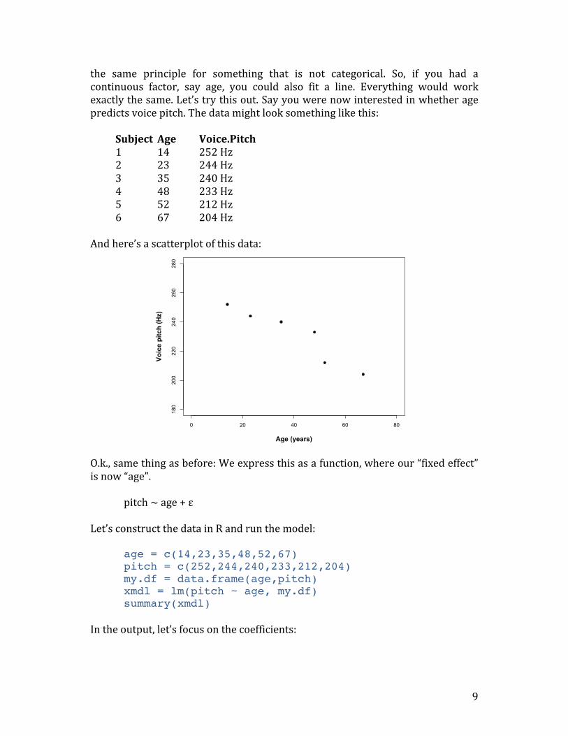
the same principle for something that is not categorical. So, if you had acontinuous factor, say age, you could also fit a line. Everything would workexactlythesame.Let’strythisout.Sayyouwerenowinterestedinwhetheragepredictsvoicepitch.Thedatamightlooksomethinglikethis: Subject Age Voice.Pitch 1 14 252Hz 2 23 244Hz 3 35 240Hz 4 48 233Hz 5 52 212Hz 6 67 204HzAndhere’sascatterplotofthisdata:

O.k.,samethingasbefore:Weexpressthisasafunction,whereour“fixedeffect”isnow“age”. pitch~age+εLet’sconstructthedatainRandrunthemodel: age = c(14,23,35,48,52,67)

pitch = c(252,244,240,233,212,204) my.df = data.frame(age,pitch) xmdl = lm(pitch ~ age, my.df) summary(xmdl)

Intheoutput,let’sfocusonthecoefficients:

0 20 40 60 80

180

200

220

240

260

280

Voic

e pi

tch

(Hz)

Age (years)

10

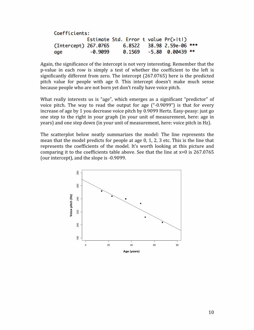
Again,thesignificanceoftheinterceptisnotveryinteresting.Rememberthatthep-value in each row is simply a test of whether the coefficient to the left issignificantlydifferent fromzero.The intercept(267.0765)here is thepredictedpitch value for people with age 0. This intercept doesn’t make much sensebecausepeoplewhoarenotbornyetdon’treallyhavevoicepitch.What really interests us is “age”,which emerges as a significant “predictor” ofvoice pitch. The way to read the output for age (“-0.9099“) is that for everyincreaseofageby1youdecreasevoicepitchby0.9099Hertz.Easy-peasy:justgoone step to the right in your graph (in your unit ofmeasurement, here: age inyears)andonestepdown(inyourunitofmeasurement,here:voicepitchinHz).The scatterplot below neatly summarizes the model: The line represents themeanthatthemodelpredictsforpeopleatage0,1,2,3etc.Thisisthelinethatrepresents the coefficients of themodel. It’s worth looking at this picture andcomparingittothecoefficientstableabove.Seethatthelineatx=0is267.0765(ourintercept),andtheslopeis-0.9099.

0 20 40 60 80

180

200

220

240

260

280

Voic

e pi

tch

(Hz)

Age (years)

11

MeaningfulandmeaninglessinterceptsYoumight want to remedy the above-discussed situation that the intercept ismeaningless. Oneway of doing thiswould be to simply subtract themean agefromeachagevalue,asisdonebelow:

my.df$age.c = my.df$age - mean(my.df$age) xmdl = lm(pitch ~ age.c, my.df) summary(xmdl)

Here,wejustcreatedanewcolumn“age.c”thatistheagevariablewiththemeansubtracted from it. This is the resulting coefficient table from running a linearmodelanalysisofthis“centered”data:

Notethatwhiletheestimatehaschangedfrom267.0765(predictedvoicepitchatage 0) to 230.8333 (predicted voice pitch at average age), the slope hasn’tchanged and neither did the significance associated with the slope or thesignificanceassociatedwiththefullmodel.Thatis,youhaven’tmessedatallwiththenatureofyourmodel,youjustchangedthemetricsothattheinterceptisnowthemeanvoicepitch.So,viacenteringourvariablewemadetheinterceptmoremeaningful.

GoingonBoth of these examples have been admittedly simple. However, things easily“scaleup” tomorecomplicatedstuff. Say,youmeasured two factors (“age”and“sex”)…youcouldputtheminthesamemodel.Yourformulawouldthenbe: pitch~sex+age+εOr,youcouldadddialectasanadditionalfactor: pitch~dialect+sex+age+εAndsoonandsoon.Theonlythingthatchangesisthefollowing.Thep-valueatthebottomoftheoutputwillbethep-valuefortheoverallmodel.Thismeansthatthe p-value considers how well all of your fixed effects together help inaccounting forvariation inpitch.Thecoefficientoutputwill thenhavep-valuesfortheindividualfixedeffects.

12

This iswhatpeoplesometimescall“multipleregression”,whereyoumodeloneresponsevariableasafunctionofmultiplepredictorvariables.Thelinearmodelisjustanotherwordformultipleregression.

Don’tstophere!!!Assumptions

There’sareasonwhywecallthelinearmodelamodel.Likeanyothermodel,thelinear model has assumptions … and it’s important to talk about theseassumptions.Sohere’sawhirlwindtourthroughtheconditionsthathavetobesatisfiedinorderforthelinearmodeltobemeaningful:(1)LinearityIt’scalled“linearmodel”forareason!Thethingtotheleftofoursimpleformulaabovehastobetheresultofalinearcombinationofthethingsontheright.Ifitdoesn’t,theresidualplotwillindicatesomekindofcurve,oritwillindicatesomeotherpattern(e.g.,twolinesifyouhavecategoricalbinarydata).Wehaven’t talkedabout residualplotsyet, letalone residuals. So, let’sdo that!Have a look at the picture below, which is a depiction of the age/pitchrelationshipagain:

0 20 40 60 80

180

200

220

240

260

280

Voic

e pi

tch

(Hz)

Age (years)

13

Theredlinesindicatetheresiduals,whicharethedeviationsoftheobserveddatapoints fromthepredictedvalues (theso-called “fittedvalues”). In thiscase, theresidualsareallfairlysmall…whichisbecausethelinethatrepresentsthelinearmodelpredictsourdataverywell,i.e.,allpointsareveryclosetotheline.Togetabetterviewof theresiduals,youcantakeasnapshotof thisgraph likethis…

… and rotate it over. So, you make a new plot where the line that the modelpredictsisnowthecenterline.Likehere:

This is a residual plot. The fitted values (the predicted means) are on thehorizontal line(aty=0).Theresidualsare theverticaldeviations fromthis line.

200 210 220 230 240 250 260

-15

-10

-50

510

15

Fitted values

Residuals

14

Thisviewisjustarotationoftheactualdata(comparetheresidualplotwiththescatterplottoseethis).Toconstructtheresidualplotforyourself,simplytype3: plot(fitted(xmdl),residuals(xmdl)) In this case… there isn’t any obvious pattern in the residuals. If therewere anonlinearor curvypattern, then thiswould indicate a violationof the linearityassumption.Here’sanexampleofaresidualplotthatclearlyshowsaviolationoflinearity:

Whattodoifyourresidualplotindicatesnonlinearity?There’sseveraloptions:

• You might miss an important fixed effect that interacts with whateverfixedeffectsyoualreadyhaveinyourmodel.Potentiallythepatternintheresidualplotgoesawayifthisfixedeffectisadded.

• Another (commonly chosen) option is to perform a nonlineartransformationofyourresponse,e.g.,bytakingthelog-transform.

• Youcanalsoperformanonlineartransformationofyourfixedeffects.So,ifageweresomehowrelatedtopitchinaU-shapedway(perhaps,ifveryyoungpeoplehadhighpitchandveryoldpeoplehadhighpitch,too,withintermediateageshavinga“dip”inpitch),thenyoucouldaddageandage2(age-squared)aspredictors.

• Finally, if you’re seeing stripes in your residual plot, then you’re mostlikelydealingwithsomekindofcategoricaldata–andyouwouldneedtoturntoasomewhatdifferentclassofmodels,suchaslogisticmodels.

3Your plotwill have no central line and itwill have different scales. It’sworth spending sometimeontweakingyourresidualplotandmakingitpretty…inparticular,youshouldmaketheplotsothatthere’smorespacearoundthemargins.Thiswillmakeanypatternseasiertosee.HavealookatsomeRgraphictutorialsforthis.

200 210 220 230 240 250 260

-15

-10

-50

510

15

Fitted values

Residuals

15

(2)AbsenceofcollinearityWhentwofixedeffects(twopredictors)arecorrelatedwitheachother,theyaresaid to be collinear. Say, you were interested in how average talking speedaffects intelligence ratings (i.e., people who talk more quickly are rated to bemoreintelligent)… intelligenceratings~talkingspeed… and youmeasured several different indicators of talking speed, for example,yoursyllablesperseconds,wordspersecondsandsentencesperseconds.Thesedifferent measures are going to be correlated with each other because if youspeakmorequickly,thenyousaymoresyllables,wordsandsentencesinagivenamountof time. If youwere touse all of these correlatedpredictors topredictintelligence ratings within the same model, you are likely going to run into acollinearityproblem.If there’s collinearity, the interpretation of the model becomes unstable:Dependingonwhichoneofcorrelatedpredictorsisinthemodel,thefixedeffectsbecome significant or cease to be significant. And, the significance of thesecorrelatedorcollinearfixedeffectsisnoteasilyinterpretable,becausetheymightstealeachother’s“explanatorypower”(that’saverycoarsewayofsayingwhat’sactuallygoingon,butyougettheidea).Intuitively, thismakes a lot of sense: Ifmultiple predictors are very similar toeachother,thenitbecomesverydifficulttodecidewhat,infact,isplayingabigrole.Howtogetridofcollinearity?Wellfirstofall,youmightpre-empttheprobleminthedesignstageofyourstudyandfocusonafewfixedeffectsthatyouknowarenotcorrelatedwitheachother.Ifyoudidn’tdothisandyouhaveseveralmultiplemeasurestochoosefromattheanalysisstageofyourstudy(e.g.,threedifferentways of measuring “talking speed”), think about which one is the mostmeaningful and drop the others (be careful here: don’t base this droppingdecision on the “significance”). Finally, youmightwant to consider dimension-reductiontechniquessuchasPrincipalComponentAnalysis.Thesecantransformseveralcorrelatedvariablesintoasmallersetofvariableswhichyoucanthenuseasnewfixedeffects.

16

(3)Homoskedasticity…or“absenceofheteroskedasticity”Being able to pronounce “heteroskedasticity” several times in a row in quicksuccession will make you a star at your next cocktail party, so go ahead andrehearsepronouncingthemnow!Jokesaside,homoskedasticityisanextremelyimportantassumption.Itsaysthatthevarianceofyourdatashouldbeapproximatelyequalacrosstherangeofyourpredicted values. If homoscedasticity is violated, you end up withheteroskedasticity,or,inotherwords,aproblemwithunequalvariances.For the homoscedasticity assumption to be met, the residuals of your modelneedtoroughlyhaveasimilaramountofdeviationfromyourpredictedvalues.Again, we can check this by looking at a residual plot. Here’s the one for theage/pitchdataagain:

There’s not really that many data points to tell whether this is reallyhomoscedastic. In this case, I would conclude that there’s not enough data tosafely determine whether there is or isn’t heteroskedasticity. Usually, I wouldconstructmodelsformuchlargerdatasetsanyway.So,here’saplotthatgivesyouanideaofhowa“good”residualplot lookswithmoredata:

200 210 220 230 240 250 260

-15

-10

-50

510

15

Fitted values

Residuals

17

Andanotherone:

Agoodresidualplotessentiallylooksblob-like.It’sagoodideatogeneratesomerandomdatatoseehowaplotwithroughlyequalvarianceslookslike.Youcandosousingthefollowingcommandline: plot(rnorm(100),rnorm(100)) Thiscreatestwosetsof100normallydistributedrandomnumberswithameanof 0 and a standard deviation of 1. If you type this inmultiple times to createmultipleplots,youcangetafeelofhowa“normal”residualplotshouldlooklike.Thenextresidualplotshowsobviousheteroskedasticity:

-3 -2 -1 0 1 2 3

-3-2

-10

12

3

Fitted values

Residuals

-3 -2 -1 0 1 2 3

-3-2

-10

12

3

Fitted values

Residuals

18

Inthisplot,higherfittedvalueshavelargerresiduals…indicatingthatthemodelismore“off”withlargerpredictedmeans.So,thevarianceisnothomoscedastic:it’ssmallerinthelowerrangeandlargerinthehigherrange.Whattodo?Again,transformingyourdataoftenhelps.Consideralog-transformhereaswell.(4)NormalityofresidualsThe normality of residuals assumption is the one that is least important.Interestingly,manypeopleseemtothinkitisthemostimportantone,butitturnsoutthatlinearmodelsarerelativelyrobustagainstviolationsoftheassumptionsofnormality.Researchersdifferwithrespecttohowmuchweighttheyputontocheckingthisassumption.Forexample,GellmanandHill(2007),afamousbookon linearmodelsandmixedmodels,donotevenrecommenddiagnosticsof thenormalityassumption(ibid.46).Ifyouwantedtotesttheassumption,howwouldyoudothis?Eitheryoumakeahistogramoftheresidualsofyourmodel,using… hist(residuals(xmdl)) …oraQ-Qplot… qqnorm(residuals(xmdl)) Here’saresidualplotandaQ-Qplotofthesameresidualsnexttoeachother.

-3 -2 -1 0 1 2 3

-3-2

-10

12

3

Fitted values

Residuals

19

These look good. The histogram is relatively bell-shaped and the Q-Q plotindicatesthatthedatafallsonastraightline(whichmeansthatit’ssimilartoanormal distribution). Here, we would conclude that there are no obviousviolationsofthenormalityassumption.(5)AbsenceofinfluentialdatapointsSomepeoplewouldn’tcall“theabsenceofinfluentialdatapoints”anassumptionof the model. However, influential data points can drastically change theinterpretationofyour results, and similar to collinearity, it can lead to instableresults.Howtocheck?Here’sausefulRfunction,dfbeta(),thatyoucanuseonamodelobjectlikeourxmdlfromabove.

For each coefficient of yourmodel (including the intercept), the function givesyoutheso-calledDFbetavalues.Thesearethevalueswithwhichthecoefficientshave to be adjusted if a particular data point is excluded (sometimes called“leave-one-outdiagnostics”).Moreconcretely,let’slookattheagecolumninthedataframeabove.Thefirstrowmeansthatthecoefficientforage(which,ifyouremember, was -0.9099) has to be adjusted by 0.06437573 if data point 1 isexcluded. Thatmeans that the coefficient of themodel without the data point

x

Frequency

-3 -2 -1 0 1 2

05

1015

20

-2 -1 0 1 2

-2-1

01

2

Normal Q-Q Plot

Theoretical Quantiles

Sam

ple

Qua

ntile

s

20

would be -0.9742451 (which is -0.9099 minus 0.06437573… if the slope isnegative,DFbetavaluesaresubtracted,ifit’spositive,theyareadded).There’salittlebitofroomforinterpretationinwhatconstitutesalargeorasmallDFbetavalue.Onethingyoucansayforsure:Anyvaluethatchangesthesignofthe slope is definitely an influential point that warrants special attention…because excluding that point would change the interpretation of your results.WhatIthendoistoeyeballtheDFbetasandlookforvaluesthataredifferentbyatleasthalfoftheabsolutevalueoftheslope.Say,myslopewouldbe2…thenaDFbetavalueof1or -1wouldbealarming tome. If it’s a slopeof -4, aDFbetavalueof2or-2wouldbealarmingtome.Howtoproceedifyouhaveinfluentialdatapoints?Well,it’sdefinitelynotlegittosimplyexcludethosepointsandreportonlytheresultsonthereduceddataset.Abetterapproachwouldbetoruntheanalysiswiththeinfluentialpointsandthenagainwithouttheinfluentialpoints…thenyoucanreportbothanalysesandstatewhether the interpretationof theresultsdoesordoesn’t change.Theonlycasewhenitiso.k.toexcludeinfluentialpointsiswhenthere’sanobviouserrorwiththem,soforexample,avaluethatdoesn’tmakesense(e.g.,negativeage,negativeheight)oravaluethatobviouslyistheresultduetoatechnicalerrorinthedataacquisitionstage(e.g.,voicepitchvaluesof0).Influencediagnosticsallowyoutospotthosepointssoyoucanthengobacktotheoriginaldataandseewhatwentwrong4.(6)Independence!!!!!!!The independence assumption is by far the most important assumption of allstatistical tests. In the linearmodelanalyses thatwedidso far,eachdatapointcame fromadifferent subject.To remindyou,here’sour twodata sets thatweworkedon: Study1 Study2 Subject Sex Voice.Pitch Subject Age Voice.Pitch 1 female 233Hz 1 14 252Hz 2 female 204Hz 2 23 244Hz 3 female 242Hz 3 35 240Hz 4 male 130Hz 4 48 233Hz 5 male 112Hz 5 52 212Hz 6 male 142Hz 6 67 204HzWewereabletorunthelinearmodelonthisdatathewaywedidonlybecauseeach row in this dataset comes from a different subject. If you elicit multiple

4For an interesting back-and-forth on a particular example of howmuch influence diagnosticsandextremevaluescanchangetheinterpretationofastudy,havealookatthedelightfulepisodeofacademicbanterbetweenUllrichandSchlüter(2011)andBrandt(2011).

21

responses from each subject, then those responses that come from the samesubjectcannotberegardedasindependentfromeachother.So,whatexactlyisindependence?Theidealcaseisacoinfliportherollofadie:Eachcoinflipandeachrollofadieisabsolutelyindependentfromtheoutcomeoftheprecedingcoinflipsordierolls.Thesameshouldholdforyourdatapointswhen you run a linear model analysis. So, the data points should come fromdifferentsubjects.Andeachsubjectshouldonlycontributeonedatapoint.Whenyouviolatetheindependenceassumption,allhellbreaksloose.Theotherassumptions that we mentioned above are important as well, but theindependence assumption is by far the most important one. Violatingindependencemaygreatlyinflateyourchanceoffindingaspuriousresultanditresults in ap-value that is completelymeaningless.Unfortunately, violationsofthe independenceassumptionarequite frequent inmanybranchesofscience–so much in fact, that there’s a whole literature associated with this violation,starting from Hurlbert (1984) for ecology, Freeberg and Lucas (2009) forpsychology, Lazic (2010) for neuroscience and my own small paper forphonetics/speechscience(Winter,2011).Howcanyouguarantee independence?Well, independence isaquestionof theexperimental design in relation to the statistical test that you use. Design andstatisticalanalysesarecloselyintertwinedandyoucanmakesurethatyoumeettheindependenceassumptionbyonlycollectingonedatapointpersubject.Now, a lot of the times, we want to collect more data per subject, such as inrepeated measures designs. If you end up with a data set that has non-independencies in it, you need to resolve these non-independencies at theanalysis stage.This iswheremixedmodels come inhandy…and this iswherewe’llswitchtothesecondtutorial.

PROCEEDTOTUTORIAL2(whichisawhirlwindtourofmixedmodels)

http://www.bodowinter.com/tutorial/bw_LME_tutorial2.pdf

22

ReferencesBrandt,M. J. (2011). Nasty data can still be real: A reply to Ullrich and Schlüter.Psychological

Science,23,826.Freeberg,T.M.,&Lucas,J.R.(2009).Pseudoreplicationis(still)aproblem.JournalofComparative

Psychology,123,450-451.Gellman, A., & Hill, J. (2007).Data analysis using regression andmultilevel/hierarchicalmodels.

Cambridge:CambridgeUniversityPress.Hurlbert,S.H.(1984).Pseudoreplicationandthedesignofecologicalfieldexperiments.Ecological

Monographs,54,187-211.Lazic,S.E.(2010).Theproblemofpseudoreplicationinneuroscientificstudies:isitaffectingyour

analysis?BMCNeuroscience,11,1-17.Ullrich, J., & Schlüter, E. (2011). Detecting nasty data with simple plots of complex models:

CommentonBrandt(2011).PsychologicalScience,23,824-825.Winter, B. (2011). Pseudoreplication in phonetic research. Proceedings of the International

CongressofPhoneticScience(pp.2137-2140).HongKong,August2011.