Linear Models I

EMBnet Course – Introduction to Statistics for Biologists 6 Mar 2007

Linear Models I

http://www.isrec.isb-sib.ch/~darlene/EMBnet/

5 10 15 20

1.0

1.2

1.4

1.6

1.8

Blood Glucose

Sho

rten

ing

Vel

ocity

Correlation and Regression


Univariate Data (Review)

Measurements on a single variable X

Consider a continuous (numerical) variable

Summarizing X

– Numerically

• Center

• Spread

– Graphically

• Boxplot

• Histogram


Bivariate Data Bivariate data are just what they sound

like – data with measurements on two variables; let’s call them X and Y

Here, we are looking at two continuous variables

Want to explore the relationship between the two variables

Can also look for association between two discrete variables; we won’t cover that here


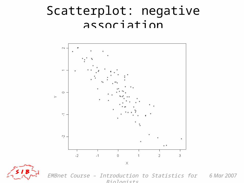
Scatterplot

We can graphically summarize a bivariate data set with a scatterplot (also sometimes called a scatter diagram)

Plots values of one variable on the horizontal axis and values of the other on the vertical axis

Can be used to see how values of 2 variables tend to move with each other (i.e. how the variables are associated)


Scatterplot: positive association


Scatterplot: negative association


Scatterplot: real data example


Numerical Summary

Typically, a bivariate data set is summarized numerically with 5 summary statistics

These provide a fair summary for scatterplots with the same general shape as we just saw, like an oval or an ellipse

We can summarize each variable separately : X mean, X SD; Y mean, Y SD

But these numbers don’t tell us how the values of X and Y vary together


Correlation Coefficient

The (sample) correlation coefficient r is defined as the average value of the product

(X in SUs)*(Y in SUs)

SU = standard units = (X – mean(X))/SD(X)

r is a unitless quantity

-1 r 1

r is a measure of LINEAR ASSOCIATION


R: correlation

In R: > cor(x,y)

Note, however, that if there are missing values (NA), then you will get an error message

Elementary statistical functions in R require

– no missing values, or

– explicit statement of what to do with NA


R: NA in statistical functions

For single vector functions (e.g. mean, var, sd), give the argument na.rm=TRUE

For cor, though, there are more possibilities for dealing with NA

See the argument use and the methods given there: ?cor


What r is...


The closer r is to –1 or 1, the more tightly the points on the scatterplot are clustered around a line

The sign of r (+ or -) is the same as the sign of the slope of the line

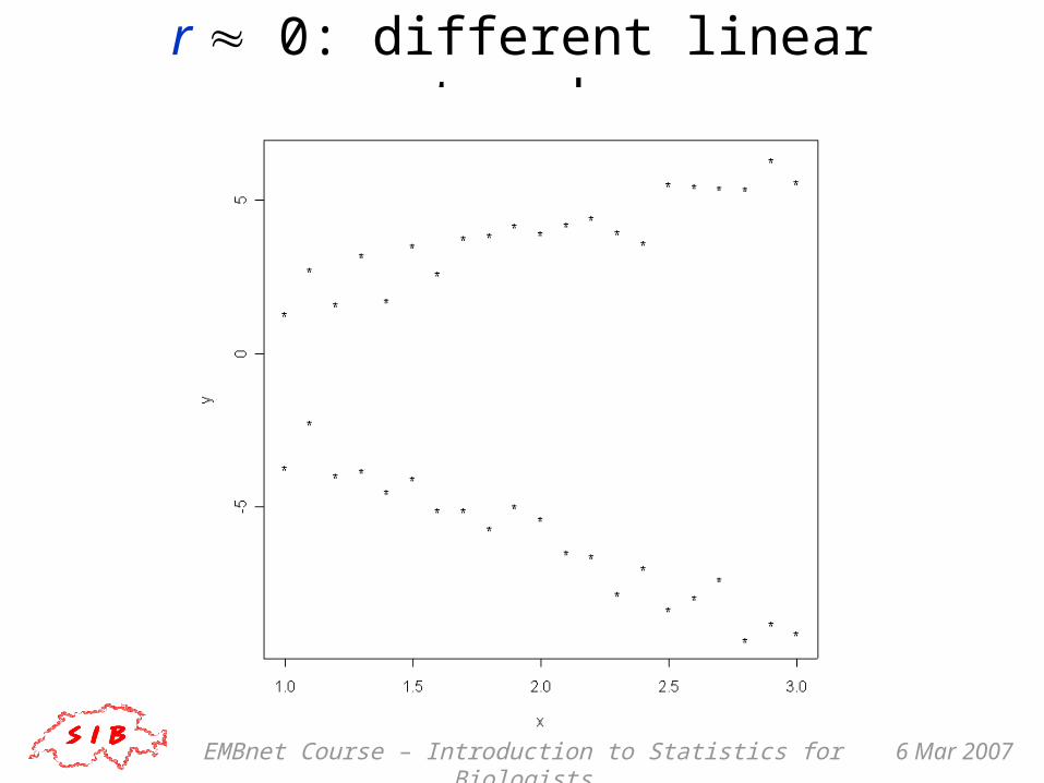
When r = 0, the points are not LINEARLY ASSOCIATED – this does NOT mean there is NO ASSOCIATION


...and what r is not


r does NOT tell us if Y is a function of X

r does NOT tell us if X causes Y

r does NOT tell us if Y causes X

r does NOT tell us what the scatterplot looks like


r 0: random scatter


r 0: curved relation


r 0: outliers

outliers


r 0: parallel lines


r 0: different linear trends


Correlation is NOT causation You cannot infer that since X and Y are

highly correlated (r close to –1 or 1) that X is causing a change in Y

Y could be causing X

X and Y could both be varying along with a third, possibly unknown factor (either causal or not; often ‘time’ ):

Polio and soft drinks: US polio cases tended to go up in summer, so do sales of soft drinks => does not mean that soft drinks cause polio


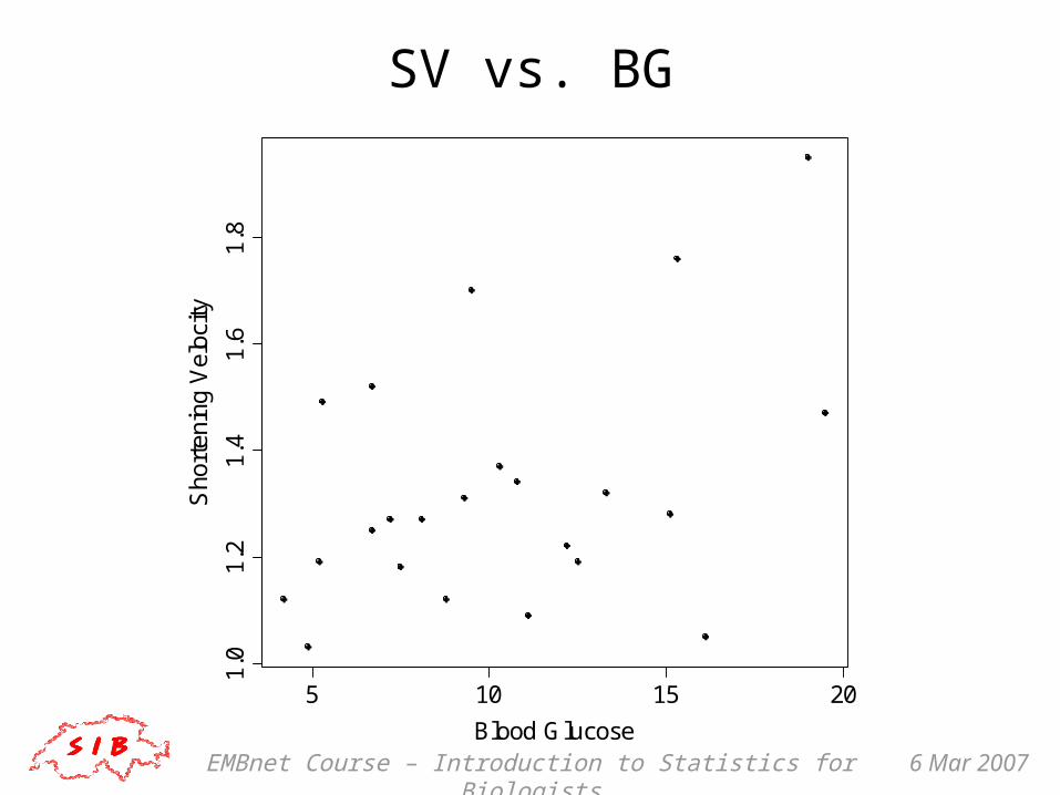
Predicting shortening velocity Say we are interested in getting a value for

shortening velocity (thuesen data)

We could measure it, but that may be difficult/expensive/impractical/etc.

If we have a measurement on a variable that is related to shortening velocity – such as blood glucose, say – then perhaps there would be some way to use that measurement to estimate or predict shortening velocity

What relation is suggested by the scatterplot?


SV vs. BG

5 10 15 20

1.0

1.2

1.4

1.6

1.8

Blood Glucose

Sho

rten

ing

Vel

ocity


(Simple) Linear Regression

Refers to drawing a (particular, special) line through a scatterplot

Used for 2 broad purposes:

– Explanation

– Prediction

Equation for a line to predict y knowing x (in slope-intercept form) looks like:

y = a + b*x

a is called the intercept ; b is the slope


Which line?

There are many possible lines that could be drawn through the cloud of points in the scatterplot ...

How to choose?


Regression Prediction The regression prediction says:

when X goes up by 1 SD, predicted Y goes up **NOT by 1 SD**, but by only r SDs (down if r is negative)

This prediction can be expressed as a formula for a line in slope-intercept form:

predicted y = intercept + slope * x,

with slope = r * SD(Y)/SD(X)

intercept = mean(Y) – slope * mean(X)


Least Squares

Q: Where does this equation come from?

A: It is the line that is ‘best’ in the sense that it minimizes the sum of the squared errors in the vertical (Y) direction

*

*

*

*

*

errors

X

Y


Interpretation of parameters

The regression line has two parameters: the slope and the intercept

The regression slope is the average change in Y when X increases by 1 unit

The intercept is the predicted value for Y when X = 0

If the slope = 0, then X does not help in predicting Y (linearly)


Another view of the regression line

We can divide the scatterplot into regions (X-strips) based on values of X

Within each X-strip, plot the average value of Y (using only Y values that have X values in the X-strip)

This is the graph of averages

The regression line can be thought of as a smoothed version of the graph of averages


Scatterplot (again)


Creating X-strips


Graph of averages


Residuals

There is an error in making a regression prediction:

error = observed Y – predicted Y

These errors are called residuals


Pitfalls in regression ecological regression

– when the units are aggregated, for example death rates from lung cancer vs. percentage of smokers in cities => relationship can look stronger than it actually is (we don’t know whether it is the smokers that are dying of lung cancer)

extrapolation– don’t know what the relationship between X

and Y looks like outside the range of the data

regression effect/fallacy– test-retest and regression toward the mean


Modeling Overview

Want to capture important features of the relationship between a (set of) variable(s) and one or more response(s)

Many models are of the form

g(Y) = f(x) + error

Differences in the form of g, f and distributional assumptions about the error term


Linear Modeling

A simple linear model:E(Y) = 0 + 1x

Gaussian measurement model:Y = 0 + 1x + ,

where ~ N(0, 2)

More generally:Y = X + ,

where Y is n x 1, X is n x p, is p x 1, is n x 1, often assumed N(0, 2Inxn)


R: linear modeling with lm To compute regression coefficients

(intercept and slope(s)) in R: lm(y ~ x) Can read ~ as ‘described (or modeled) by ’

Example : to predict ventricular shortening velocity from blood glucose:

> lm(short.velocity ~ blood.glucose) Call:lm(formula = short.velocity ~ blood.glucose)Coefficients: (Intercept) blood.glucose 1.09781 0.02196


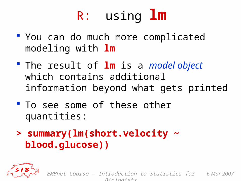
R: using lm You can do much more complicated

modeling with lm

The result of lm is a model object which contains additional information beyond what gets printed

To see some of these other quantities:

> summary(lm(short.velocity ~ blood.glucose))


R: summarizing lm> summary(lm(short.velocity~blood.glucose))Call:lm(formula = short.velocity ~ blood.glucose)

Residuals: Min 1Q Median 3Q Max -0.40141 -0.14760 -0.02202 0.03001 0.43490

Coefficients: Estimate Std. Error t value Pr(>|t|) (Intercept) 1.09781 0.11748 9.345 6.26e-09 ***blood.glucose 0.02196 0.01045 2.101 0.0479 * ---Signif. codes: 0 `***' 0.001 `**' 0.01 `*' 0.05 `.' 0.1

` ' 1

Residual standard error: 0.2167 on 21 degrees of freedomMultiple R-Squared: 0.1737, Adjusted R-squared: 0.1343 F-statistic: 4.414 on 1 and 21 DF, p-value: 0.0479


Basic model checking

Examination of residuals– Normality– Time effects– Nonconstant variance– Curvature

Detection of influential observations– Hat matrix

We will do a little of this in the practical


QQ-Plot Quantile-quantile plot

Assess whether a sample follows a particular (e.g. normal) distribution (or to compare two samples)

A method for looking for outliers when data are mostly normal

Sam

ple

Theoretical

Sample quantile is 0.125

Value from Normal distribution which yields a quantile of 0.125 (= -1.15)


Typical deviations from straight line patterns

Outliers

Curvature at both ends (long or short tails)

Convex/concave curvature (asymmetry)

Horizontal segments, plateaus, gaps


Outliers


Long Tails


Short Tails


Asymmetry


Plateaus/Gaps


Hat values

High leverage points are far from the center, and have potentially greater influence

One way to assess points is through the hat values (obtained from the hat matrix H):

ŷ = Xb = X(X’X)-1X’y = Hy

hi = Σjhij2

Average value of h = number of coefficients/n (including the intercept) = p/n

Cutoff typically 2p/n or 3p/n


CIs and hypothesis tests

With some assumptions about the error distribution, you can make confidence intervals or carry out hypothesis tests :

– for the regression line

– prediction interval for future observation

– hypothesis tests for coefficients

We will not worry about the details of these

Linear Models I

Documents

Transcript of Linear Models I