Linear Algebra I - Oregon Institute of Technologymath.oit.edu/~watermang/341book.pdf · 2.3...
213
Linear Algebra I Gregg Waterman Oregon Institute of Technology
Transcript of Linear Algebra I - Oregon Institute of Technologymath.oit.edu/~watermang/341book.pdf · 2.3...

Linear Algebra I
Gregg WatermanOregon Institute of Technology

c©2016 Gregg Waterman
This work is licensed under the Creative Commons Attribution-NonCommercial-ShareAlike 3.0 UnportedLicense. The essence of the license is that
You are free:
• to Share to copy, distribute and transmit the work
• to Remix to adapt the work
Under the following conditions:
• Attribution You must attribute the work in the manner specified by the author (but not inany way that suggests that they endorse you or your use of the work). Please contact the authorat [email protected] to determine how best to make any attribution.
• Noncommercial You may not use this work for commercial purposes.
• Share Alike If you alter, transform, or build upon this work, you may distribute the resultingwork only under the same or similar license to this one.
With the understanding that:
• Waiver Any of the above conditions can be waived if you get permission from the copyrightholder.
• Public Domain Where the work or any of its elements is in the public domain under applicablelaw, that status is in no way affected by the license.
• Other Rights In no way are any of the following rights affected by the license:
⋄ Your fair dealing or fair use rights, or other applicable copyright exceptions and limitations;
⋄ The author’s moral rights;
⋄ Rights other persons may have either in the work itself or in how the work is used, such aspublicity or privacy rights.
• Notice For any reuse or distribution, you must make clear to others the license terms of thiswork. The best way to do this is with a link to the web page below.
To view a full copy of this license, visit http://creativecommons.org/licenses/by-nc-sa/3.0/ or send a letterto Creative Commons, 444 Castro Street, Suite 900, Mountain View, California, 94041, USA.

Contents
0 Introduction 1
1 Systems of Linear Equations 31.1 Linear Equations and Systems of Linear Equations . . . . . . . . . . . . . . . . . . . 41.2 The Addition Method . . . . . . . . . . . . . . . . . . . . . . . . . . . . . . . . . . . 51.3 Solving With Matrices . . . . . . . . . . . . . . . . . . . . . . . . . . . . . . . . . . . 91.4 Applications: Curve Fitting and Temperature Equilibrium . . . . . . . . . . . . . . . 141.5 Chapter 1 Exercises . . . . . . . . . . . . . . . . . . . . . . . . . . . . . . . . . . . . 18
2 More on Systems of Linear Equations 232.1 “When Things Go Wrong” . . . . . . . . . . . . . . . . . . . . . . . . . . . . . . . . 242.2 Overdetermined and Underdetermined Systems . . . . . . . . . . . . . . . . . . . . . 302.3 Application: Network Analysis . . . . . . . . . . . . . . . . . . . . . . . . . . . . . . 312.4 Approximating Solutions With Iterative Methods . . . . . . . . . . . . . . . . . . . . 332.5 Chapter 2 Exercises . . . . . . . . . . . . . . . . . . . . . . . . . . . . . . . . . . . . 37
3 Euclidean Space and Vectors 433.1 Euclidean Space . . . . . . . . . . . . . . . . . . . . . . . . . . . . . . . . . . . . . . 443.2 Introduction to Vectors . . . . . . . . . . . . . . . . . . . . . . . . . . . . . . . . . . 473.3 Addition and Scalar Multiplication of Vectors, Linear Combinations . . . . . . . . . 493.4 The Dot Product of Vectors, Projections . . . . . . . . . . . . . . . . . . . . . . . . . 553.5 Chapter 3 Exercises . . . . . . . . . . . . . . . . . . . . . . . . . . . . . . . . . . . . 59
4 Vectors and Systems of Equations 614.1 Linear Combination Form of a System . . . . . . . . . . . . . . . . . . . . . . . . . . 624.2 Sets of Vectors . . . . . . . . . . . . . . . . . . . . . . . . . . . . . . . . . . . . . . . 654.3 Vector Equations of Lines and Planes . . . . . . . . . . . . . . . . . . . . . . . . . . 694.4 Interpreting Solutions to Systems of Linear Equations . . . . . . . . . . . . . . . . . 744.5 Chapter 4 Exercises . . . . . . . . . . . . . . . . . . . . . . . . . . . . . . . . . . . . 77
5 Matrices and Vectors 795.1 Introduction . . . . . . . . . . . . . . . . . . . . . . . . . . . . . . . . . . . . . . . . . 805.2 Multiplying a Matrix Times a Vector . . . . . . . . . . . . . . . . . . . . . . . . . . . 835.3 Actions of Matrices on Vectors: Transformations in R
2 . . . . . . . . . . . . . . . . 875.4 Chapter 5 Exercises . . . . . . . . . . . . . . . . . . . . . . . . . . . . . . . . . . . . 94
6 Matrix Multiplication 956.1 Multiplying Matrices . . . . . . . . . . . . . . . . . . . . . . . . . . . . . . . . . . . . 966.2 More Multiplying Matrices . . . . . . . . . . . . . . . . . . . . . . . . . . . . . . . . 1026.3 Inverse Matrices . . . . . . . . . . . . . . . . . . . . . . . . . . . . . . . . . . . . . . 1066.4 Applications of Matrices II: Rotations and Projections, Graph Theory . . . . . . . . 1106.5 Chapter 6 Exercises . . . . . . . . . . . . . . . . . . . . . . . . . . . . . . . . . . . . 113
7 Matrices and Systems of Equations 1157.1 Matrix Equation Form of a System . . . . . . . . . . . . . . . . . . . . . . . . . . . . 1167.2 Solving a System With An LU -Factorization . . . . . . . . . . . . . . . . . . . . . . 1187.3 Inverse Matrices and Systems . . . . . . . . . . . . . . . . . . . . . . . . . . . . . . . 1217.4 Determinants and Matrix Form . . . . . . . . . . . . . . . . . . . . . . . . . . . . . . 1237.5 Homogeneous Systems . . . . . . . . . . . . . . . . . . . . . . . . . . . . . . . . . . . 1277.6 Chapter 7 Exercises . . . . . . . . . . . . . . . . . . . . . . . . . . . . . . . . . . . . 128
i
8 Vector Spaces and Subspaces 1298.1 Span of a Set of Vectors . . . . . . . . . . . . . . . . . . . . . . . . . . . . . . . . . . 1308.2 Closure of a Set Under an Operation . . . . . . . . . . . . . . . . . . . . . . . . . . . 1358.3 Vector Spaces and Subspaces . . . . . . . . . . . . . . . . . . . . . . . . . . . . . . . 1378.4 Column Space and Null Space of a Matrix . . . . . . . . . . . . . . . . . . . . . . . . 1448.5 Least Squares Solutions to Inconsistent Systems . . . . . . . . . . . . . . . . . . . . . 1478.6 Chapter 8 Exercises . . . . . . . . . . . . . . . . . . . . . . . . . . . . . . . . . . . . 151
9 Bases of Subspaces 1539.1 Linear Independence . . . . . . . . . . . . . . . . . . . . . . . . . . . . . . . . . . . . 1549.2 Bases of Subspaces, Dimension . . . . . . . . . . . . . . . . . . . . . . . . . . . . . . 1609.3 Bases for the Column Space and Null Space of a Matrix . . . . . . . . . . . . . . . . 1649.4 Solutions to Systems of Equations . . . . . . . . . . . . . . . . . . . . . . . . . . . . 1689.5 Chapter 9 Exercises . . . . . . . . . . . . . . . . . . . . . . . . . . . . . . . . . . . . 170
10 Linear Transformations 17310.1 Transformations of Vectors . . . . . . . . . . . . . . . . . . . . . . . . . . . . . . . . 17410.2 Linear Transformations . . . . . . . . . . . . . . . . . . . . . . . . . . . . . . . . . . 17610.3 Compositions of Transformations . . . . . . . . . . . . . . . . . . . . . . . . . . . . . 18310.4 Chapter 10 Exercises . . . . . . . . . . . . . . . . . . . . . . . . . . . . . . . . . . . . 186
11 Eigenvalues, Eigenspaces and Diagonalization 18711.1 An Introduction to Eigenvalues and Eigenvectors . . . . . . . . . . . . . . . . . . . . 18811.2 Finding Eigenvalues and Eigenvectors . . . . . . . . . . . . . . . . . . . . . . . . . . 19211.3 Diagonalization of Matrices . . . . . . . . . . . . . . . . . . . . . . . . . . . . . . . . 19611.4 Solving Systems of Differential Equations . . . . . . . . . . . . . . . . . . . . . . . . 199
A Index of Symbols 201
B Solutions to Exercises 203B.1 Chapter 1 Solutions . . . . . . . . . . . . . . . . . . . . . . . . . . . . . . . . . . . . 203B.2 Chapter 2 Solutions . . . . . . . . . . . . . . . . . . . . . . . . . . . . . . . . . . . . 204B.3 Chapter 3 Solutions . . . . . . . . . . . . . . . . . . . . . . . . . . . . . . . . . . . . 204B.4 Chapter 4 Solutions . . . . . . . . . . . . . . . . . . . . . . . . . . . . . . . . . . . . 206B.5 Chapter 5 Solutions . . . . . . . . . . . . . . . . . . . . . . . . . . . . . . . . . . . . 207B.6 Chapter 6 Solutions . . . . . . . . . . . . . . . . . . . . . . . . . . . . . . . . . . . . 208B.7 Chapter 7 Solutions . . . . . . . . . . . . . . . . . . . . . . . . . . . . . . . . . . . . 209B.8 Chapter 8 Solutions . . . . . . . . . . . . . . . . . . . . . . . . . . . . . . . . . . . . 211B.9 Chapter 9 Solutions . . . . . . . . . . . . . . . . . . . . . . . . . . . . . . . . . . . . 212B.10 Chapter 10 Solutions . . . . . . . . . . . . . . . . . . . . . . . . . . . . . . . . . . . . 214
ii
0 Introduction
This book is an attempt to make the subject of linear algebra as understandable as possible, for afirst time student of the subject. I developed the book from a set of notes used to supplement astandard textbook used when I taught the course in the past. At the end of the term I surveyedthe students in the class, and the vast majority of them thought that the supplemental notes thatI had provided would have been an adequate resource for them to learn the subject. Encouragedby this, I put further work in to correcting errors, adding examples and including material that Ihad left to the textbook previously. Here is the result, in its fourth edition.
You should look at the table of contents and page through the book a bit at first to see howit is organized. Note in particular that each section begins with statements of the performancecriteria addressed in that section. Performance criteria are the specific things that you will beexpected to do in order to demonstrate your skills and your understanding of concepts. Withineach section you will find examples relating to those performance criteria, and at the end of eachchapter are exercises for you to practice your skills and test your understanding.
It is my belief that you will likely forget many of the details of this course after you leave it, so itmight seem that developing the ability to perform the tasks outlined in the performance criteria isin vain. That causes me no dismay, nor should it you! My first goal is for you to learn the materialwell enough that if you are required to recall or relearn it in other courses you can do so easilyand quickly, and along the way I hope that you develop an appreciation for the subject of linearalgebra. Most of all, my aim is for you to develop your skills beyond their current level in the areasof mathematical reasoning and communication. In support of that, you will find the first (well,“zeroth”!) outcome and its associated performance criteria below. Outcomes are statements ofgoals that are perhaps a bit nebulous, and difficult to measure directly. The performance criteriagive specific, measurable tasks by which success in the overarching outcome can be determined.
Learning Outcome:
0. Use the subject of linear algebra to develop sophistication in understandingof mathematical concepts and connections, and in the communication ofthat understanding.
Performance Criteria:
(a) Apply skills and knowledge associated with specific performance cri-teria to problems related to, but not specifically addressed by, thoseperformance criteria.
(b) Communicate mathematical ideas clearly by correctly using writtenEnglish and proper mathematical notation.
Enough talk - let’s get to it!
Gregg WatermanFebruary 2016
1

2

1 Systems of Linear Equations
Learning Outcome:
1. Solve systems of linear equations using Gaussian elimination, use systemsof linear equations to solve problems.
Performance Criteria:
(a) Determine whether an equation in n unknowns is linear.
(b) Determine what the solution set to a linear equation represents geo-metrically.
(c) Determine whether an n-tuple is a solution to a linear equation or asystem of linear equations.
(d) Solve a system of two linear equations by the addition method.
(e) Find the solution to a system of two linear equations in two unknownsgraphically.
(f) Give the coefficient matrix and augmented matrix for a system ofequations.
(g) Determine whether a matrix is in row-echelon form. Perform, byhand, elementary row operations to reduce a matrix to row-echelonform.
(h) Determine whether a matrix is in reduced row-echelon form. Usea calculator or software to reduce a matrix to reduced row-echelonform.
(i) For a system of equations having a unique solution, determine thesolution from either the row-echelon form or reduced row-echelon formof the augmented matrix for the system.
(j) Use a calculator to solve a system of linear equations having a uniquesolution.
(k) Use systems of equations to solve curve fitting and temperature equi-librium problems.
3

1.1 Linear Equations and Systems of Linear Equations
Performance Criteria:
1. (a) Determine whether an equation in n unknowns is linear.
(b) Determine what the solution set to a linear equation represents geo-metrically.
(c) Determine whether an n-tuple is a solution to a linear equation or asystem of linear equations.
Linear Equations and Their Solutions
It is natural to begin our study of linear algebra with the process of solving systems of linearequations, and applications of such systems. Linear equations are ones of the form
2x−3y = 7 5.3x+7.2y+1.4z = 15.9 a11x1+a12x2+ · · ·+a1(n−1)xn−1+a1nxn = b1
where x, y, z, x1, ..., xn are all unknown values. In the third example, a11, a12, ..., a1n, b1 areall known numbers, just like the values 2, −3, 5.3, 7.2, 1.4 and 15.9. Although you may haveused x and y, or x, y and z as the unknown quantities in the past, we will often use x1,x2, ..., xn. One obvious advantage to this is that we don’t have to fret about what letters to use,and there is no danger of running out of letters! You will eventually see that there is also a verygood mathematical reason for using just x (or some other single letter), with subscripts denotingdifferent values.
When we look at two or more linear equations together “as a package,” the result is somethingcalled a system of linear equations. Here are a couple of examples:
x+ 3y − 2z = −43x+ 7y + z = 4
−2x+ y + 7z = 7
a11x1 + a12x2 + · · ·+ a1,n−1xn−1 + a1nxn = b1
a21x1 + a22x2 + · · ·+ a2,n−1xn−1 + a2nxn = b2
......
am1x1 + am2x2 + · · ·+ am,n−1xn−1 + amnxn = bm
The system above and to the left is a system of three equations in three unknowns. We will spenda lot of time with such systems because they exhibit just about everything that we would like tosee but are small enough to be manageable to work with. The second system above is a generalsystem of m equations in n unknowns. m and n need not be the same, and either can be largerthan the other.
Our objective when dealing with a system of linear equations is usually to solve the system,which means to find a set of values for the unknowns for which all of the equations are true. Ifwe find such a set, it is called a solution to the system of equations. A solution is then a listof numbers, in order, which can be substituted for x1, x2, ... to make EVERY equation in thesystem true. In some cases there is more than one such set, so there can be many solutions, andsometimes a system of equations will have no solution. That is, there is no set of values for x1,x2, ... that makes every one of the equations in the system true.
4

1.2 The Addition Method
Performance Criteria:
1. (d) Solve a system of two linear equations by the addition method.
(e) Find the solution to a system of two linear equations in two unknownsgraphically.
Consider the systemx− 3y = 6
−2x+ 5y = −5 of linear equations. In this case a solution to the
system is an ordered pair (x, y) that makes both equations true. A large part of linear algebraconcerns itself with methods of solving such systems, and ways of interpreting solutions or lack ofsolutions.
In the past you should have learned two methods for solving such systems, the additionmethod and the substitution method. The method we want to focus on is the addition method.In this case we could multiply the first equation by two and add the resulting equation to the sec-
ond. (The first equation itself is left alone.) The result isx− 3y = 6−y = 7
; from this we can see
that y = −7. This value is then substituted into the first equation to get x = −15.Sometimes we have to do something a little more complicated:
⋄ Example 1.2(a): Solve the system2x− 4y = 183x+ 5y = 5
using the addition method.
Here we can eliminate x by multiplying the first equation by 3 and the second by −2, thenadding:
2x− 4y = 183x+ 5y = 5
=⇒ 6x− 12y = 54−6x− 10y = −10
−22y = 44
y = −2Now we can substitute this value of y back into either equation to find x:
2x− 4(−2) = 182x+ 8 = 18
2x = 10x = 5
The solution to the system is then x = 5, y = −2, which we usually write as the ordered pair(5,−2). It can be easily verified that this pair is a solution to both equations.
It is useful for the future to understand a way to multiply only one equation by a factor beforeadding. In the next example we see how that is done, using the same system of equations as inExample 1.2(a).
5
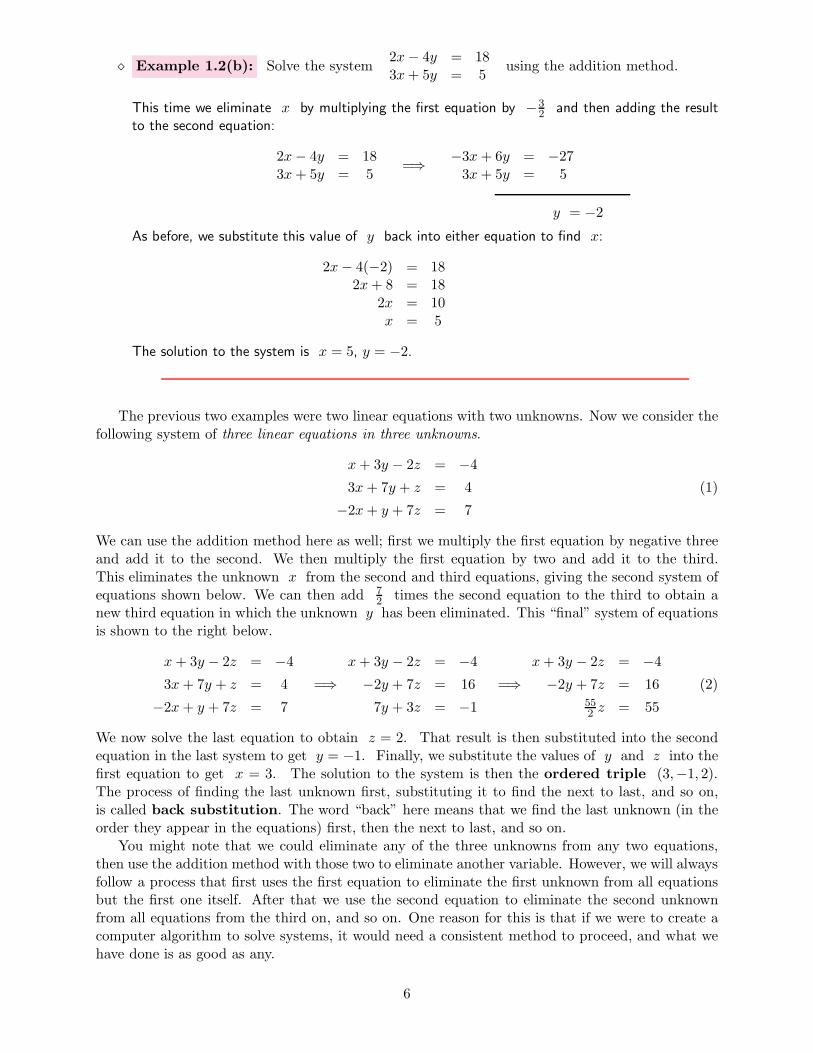
⋄ Example 1.2(b): Solve the system2x− 4y = 183x+ 5y = 5
using the addition method.
This time we eliminate x by multiplying the first equation by −32 and then adding the result
to the second equation:
2x− 4y = 183x+ 5y = 5
=⇒ −3x+ 6y = −273x+ 5y = 5
y = −2As before, we substitute this value of y back into either equation to find x:
2x− 4(−2) = 182x+ 8 = 18
2x = 10x = 5
The solution to the system is x = 5, y = −2.
The previous two examples were two linear equations with two unknowns. Now we consider thefollowing system of three linear equations in three unknowns.
x+ 3y − 2z = −43x+ 7y + z = 4
−2x+ y + 7z = 7
(1)
We can use the addition method here as well; first we multiply the first equation by negative threeand add it to the second. We then multiply the first equation by two and add it to the third.This eliminates the unknown x from the second and third equations, giving the second system ofequations shown below. We can then add 7
2 times the second equation to the third to obtain anew third equation in which the unknown y has been eliminated. This “final” system of equationsis shown to the right below.
x+ 3y − 2z = −43x+ 7y + z = 4
−2x+ y + 7z = 7
=⇒x+ 3y − 2z = −4−2y + 7z = 16
7y + 3z = −1=⇒
x+ 3y − 2z = −4−2y + 7z = 16
552 z = 55
(2)
We now solve the last equation to obtain z = 2. That result is then substituted into the secondequation in the last system to get y = −1. Finally, we substitute the values of y and z into thefirst equation to get x = 3. The solution to the system is then the ordered triple (3,−1, 2).The process of finding the last unknown first, substituting it to find the next to last, and so on,is called back substitution. The word “back” here means that we find the last unknown (in theorder they appear in the equations) first, then the next to last, and so on.
You might note that we could eliminate any of the three unknowns from any two equations,then use the addition method with those two to eliminate another variable. However, we will alwaysfollow a process that first uses the first equation to eliminate the first unknown from all equationsbut the first one itself. After that we use the second equation to eliminate the second unknownfrom all equations from the third on, and so on. One reason for this is that if we were to create acomputer algorithm to solve systems, it would need a consistent method to proceed, and what wehave done is as good as any.
6

Geometric Interpretation
At the start of this section we saw that the systemx− 3y = 6
−2x+ 5y = −5 has the solution
(−15,−7). You should be aware that if we graph the equation x − 3y = 6 we get a line.Technically speaking, what we have graphed is the solution set, the set of all pairs (x, y) thatmake the equation true. Any pair (x, y) of numbers that makes the equation true is on the line,and the (x, y) representing any point on the line will make the equation true. If we plot the
solution sets of both equations in the systemx− 3y = 6
−2x+ 5y = −5 together in the coordinate
plane we will get two lines. Since (−15,−7) is a solution to both equations, the two lines crossat the point with those coordinates! We could use this idea to (somewhat inefficiently and possiblyinaccurately) solve a system of two equations in two unknowns:
⋄ Example 1.2(c): Solve the system2x− 3y = −63x− y = 5
graphically.
We begin by solving each of the equations for y; this will giveus the equations in y = mx+ b form, for easy graphing. Theresults are
y = 23x+ 2 and y = 3x− 5
If we graph these two equations on the same graph, we get thepicture to the right. Note that the two lines cross at the point(3, 4), so the solution to the system of equations is (3, 4), orx = 3, y = 4.
5
5
-5
-5
y = 2
3x+ 2
y = 3x− 5
(3, 4)
x
y
Now consider the systemx+ 3y − 2z = −43x+ 7y + z = 4
−2x+ y + 7z = 7
having solution (3,−1, 2). What is the geometric interpretation of this? Since there are threeunknowns, the appropriate geometric setting is three-dimensional space. The solution set to anyequation ax + by + cz = d is a plane, as long as not all of a, b and c are zero. Therefore,a solution to the system is a point that lies on each of the planes representing the solution sets ofthe three equations. For our example, then, the planes representing the three equations intersectat the point (3,−1, 2).
It is possible that two lines in the standard two-dimensional plane might be parallel; in thatcase a system consisting of the two equations representing those lines will have no solution. It isalso possible that two equations might actually represent the same line, in which case the systemconsisting of those two equations will have infinitely many solutions. Investigation of those twocases will lead us to more complex considerations that we will avoid for now.
In the study of linear algebra we will be defining new concepts and developing correspondingnotation. We begin the development of notation with the following. The set of all real numbersis denoted by R, and the set of all ordered pairs of real numbers is R
2, spoken as “R-two.”Geometrically, R
2 is the familiar Cartesian coordinate plane. Similarly, the set of all orderedtriples of real numbers is the three-dimensional space referred to as R
3, “R-three.”
7

All of the algebra that we will be doing using equations with two or three unknowns can easilybe done with more unknowns. In general, when we are working with n unknowns, we will getsolutions that are n-tuples of numbers. Any such n-tuple represents a location in n-dimensionalspace, denoted R
n. Note that a linear equation in two unknowns represents a line in R2, in
the sense that the set of solutions to the equation forms a line. We consider a line to be a one-dimensional object, so the linear equation represents a one-dimensional object in two-dimensionalspace. The solution set to a linear equation in three unknowns is a plane in three-dimensionalspace. The plane itself is two-dimensional, so we have a two-dimensional “flat” object in threedimensional space.
Similarly, when we consider the solution set of a linear equation in n unknowns, its solutionset represents an n − 1-dimensional “flat” object in n-dimensional space. When such an objecthas more than two dimensions, we usually call it a hyperplane. Although such objects can’t bevisualized, they certainly exist in a mathematical sense.
Section 1.2 Exercises
1. Solve each of the following systems by the addition method.
(a)2x− 3y = −7−2x+ 5y = 9
(b)2x− 3y = −63x− y = 5
(c)4x+ y = 14
2x+ 3y = 12
(d)7x− 6y = 13
6x− 5y = 11(e)
5x+ 3y = 7
3x− 5y = −23(f)
5x− 3y = −117x+ 6y = −12
2. Solve each of the following systems by graphing, as done in Example 1.2(b).
(a)3x− 4y = 8
x+ 2y = 6(b)
4x− 3y = 9
x+ 2y = −6(c)
5x+ y = 12
7x− 2y = 10
8

1.3 Solving With Matrices
Performance Criteria:
1. (f) Give the coefficient matrix and augmented matrix for a system ofequations.
(g) Determine whether a matrix is in row-echelon form. Perform, byhand, elementary row operations to reduce a matrix to row-echelonform.
(h) Determine whether a matrix is in reduced row-echelon form. Usea calculator or software to reduce a matrix to reduced row-echelonform.
(f) For a system of equations having a unique solution, determine thesolution from either the row-echelon form or reduced row-echelon formof the augmented matrix for the system.
(g) Use a calculator to solve a system of linear equations having a uniquesolution.
Note that when using the addition method for solving the system of three equations in threeunknowns in the previous section, the symbols x, y and z and the equal signs are simply“placeholders” that are “along for the ride.” To make the process cleaner we can simply arrangethe constants a, b, c and d for each equation ax+ by+ cz = d in an array form called a matrix,which is simply a table of values like
1 3 −2 −43 7 1 4−2 1 7 7
.
Each number in a matrix is called an entry of the matrix. Each horizontal line of numbers ina matrix is a row of the matrix, and each vertical line of numbers is a column. The size ordimensions of a matrix is (are) given by giving first the number of rows, then the number ofcolumns, with the × symbol between them. The size of the above matrix is 3× 4, which we sayas “three by four.”
Suppose that the above matrix came from the system of equations
x+ 3y − 2z = −43x+ 7y + z = 4
−2x+ y + 7z = 7
When a matrix represents a system of equations, as this one does, it is called the augmentedmatrix of the system. The matrix consisting of just the coefficients of x, y and z from eachequation is called the coefficient matrix:
1 3 −23 7 1−2 1 7
We are not interested in the coefficient matrix at this time, but we will be later. The reason forthe name “augmented matrix” will also be seen later.
9

Once we have the augmented matrix, we can perform a process called row-reduction, whichis essentially what we did in the previous section, but we work with just the matrix rather thanthe system of equations. The following example shows how this is done for the above matrix.
⋄ Example 1.3(a): Solve the system (1) from the previous section by row-reduction.
We begin by adding negative three times the first row to the second, and put the result in thesecond row. Then we add two times the first row to the third, and place the result in the third.Using the notation Rn (not to be confused with R
n!) to represent the nth row of the matrix,we can symbolize these two operations as shown in the middle below. The matrix to the rightbelow is the result of those operations.
1 3 −2 −43 7 1 4−2 1 7 7
−3R1 +R2 → R2
=⇒2R1 +R3 → R3
1 3 −2 −40 −2 7 160 7 3 −1
Next we finish with the following:
1 3 −2 −40 −2 7 160 7 3 −1
72R2 + 2R3 → R3
=⇒
1 3 −2 −40 −2 7 160 0 55
2 55
The process just outlined is called row reduction. At this point we return to the equation form
x+ 3y − 2z = −40x− 2y + 7z = 16
0x+ 0y + 55z = 110
and perform back-substitution as before (see the top of page 6) to obtain z = 2, y = −1 andx = 3.
The final form of the matrix before we went back to equation form is something called row-echelon form. (The word “echelon” is pronounced “esh-el-on.”) The first non-zero entry in eachrow is called a leading entry; in this case the leading entries are the numbers 1, −2 and 55
2 .To be in row-echelon form means that
• any rows containing all zeros are at the bottom of the matrix and
• the leading entry in any row is to the right of any leading entries above it.
⋄ Example 1.3(b): Which of the matrices below are in row-echelon form?
1 3 −2 −40 0 3 −50 7 −10 −1
2 6 −1 9 50 0 −8 1 −30 0 0 0 2
7 −12 5 00 0 0 00 −5 1 8
The leading entries of the rows of the first matrix are 1, 3 and 7. Because the leading entry ofthe third row (7) is not to the right of the leading entry of the second row (3), the first matrixis not in row-echelon form. In the third matrix, there is a row of zeros that is not at the bottomof the matrix, so it is not in row-reduced form. The second matrix is in row-reduced form.
10

It is possible to continue with the matrix operations to obtain something called reduced row-echelon form, from which it is easier to find the values of the unknowns. The requirements forbeing in reduced row-echelon form are the same as for row-echelon form, with the addition of thefollowing:
• All leading entries are ones.
• The entries above any leading entry are all zero except perhaps in the last column.
Obtaining reduced row-echelon form requires more matrix manipulations, and nothing is reallygained by obtaining that form if you are doing this by hand. However, when using software ora calculator it is most convenient to obtain reduced row-echelon form. Here are two examples ofmatrices in reduced row-echelon form:
1 0 0 30 1 0 −70 0 1 4
1 6 0 9 50 0 1 2 −30 0 0 0 1
For the first matrix above, one can easily see that if it came from the augmented matrix of a systemof three equations in three unknowns, then (3,−7, 4) would be the solution to the system. Wewill have to wait a bit before we are ready to interpret what the second matrix would be telling usif it came from a system of equations.
Occasionally we need to exchange two rows when performing row-reduction. The followingexample shows a situation in which this applies.
⋄ Example 1.3(c): Row-reduce the matrix
1 3 −2 −42 6 −1 −13−1 4 −8 3
.
We begin by adding negative two times the first row to the second, and put the result in thesecond row. Then we add two times the first row to the third, and place the result in the third.Using the notation Rn (not to be confused with R
n!) to represent the nth row of the matrix,we can symbolize these two operations as shown in the middle below. The matrix to the rightbelow is the result of those operations.
1 3 −2 −42 6 −1 −13−1 4 −8 3
−2R1 +R2 → R2
=⇒R1 +R3 → R3
1 3 −2 −40 0 3 −50 7 −10 −1
We can see that the matrix would be in row-echelon form is we simply switched the second andthird rows (which is equivalent to simply rearranging the order of our original equations), so that’swhat we do:
1 3 −2 −40 0 3 −50 7 −10 −1
R2 ←→ R3
=⇒
1 3 −2 −40 7 −10 −10 0 3 −5
The act of rearranging rows in a matrix is called permuting them. In general, a permutation ofa set of objects is simply a rearrangement of them.
11

Row Reduction Using Technology
The two technologies that we will use in this course are your graphing calculator and thecomputer software called MATLAB. The row reduction process can be done on a TI-83 calculatoras follows; if you have a different calculator you will need to refer to your user’s manual to find outhow to do this. Practice using the matrix from the Example 1.3(a).
• Find and press the MATRIX (or maybe MATRX) key.
• Select EDIT. At that point you will see something like 3× 3 somewhere. This is the numberof rows and columns your matrix is going to have. We want 3× 4.
• After you have told the calculator that you want a 3× 4 matrix, it will begin prompting youfor the entries in the matrix, starting in the upper left corner. Here you will begin enteringthe values from the augmented matrix, row by row. You should see the entries appear in amatrix as you enter them.
• After you enter the matrix, you need to get to MATH under the MATRIX menu. Select rref(for reduced row-echelon form) and you should see rref ( on your calculator screen.
• Select NAMES under the MATRIX menu. Highlight A and hit enter, then enter again.
• Pick off the values of x, y and z, or x1, x2 and x3, depending on notation. Use thesame letters as are given in the exercise you are doing.
We will put off learning how to do this with MATLAB until we have some more things we cando with it as well, but the command is the same. Only the method for entering the matrix differs.
Section 1.3 Exercises
1. Give the coefficient matrix and augmented matrix for the system of equations
x + y − 3z = 1
−3x+ 2y − z = 7
2x+ y − 4z = 0
.
2. Determine which of the following matrices are in row-echelon form.
A =
[
3 −7 5 0 2 −40 0 0 −2 5 −1
]
B =
1 0 0 40 1 0 −20 0 3 5
C =
0 0 4 40 1 −3 26 1 3 5
D =
1 3 −5 10 −70 0 1 0 20 0 0 1 −40 0 0 0 20 0 0 0 0
3. Determine which of the matrices in Exercise 2 are in reduced row-echelon form.
12
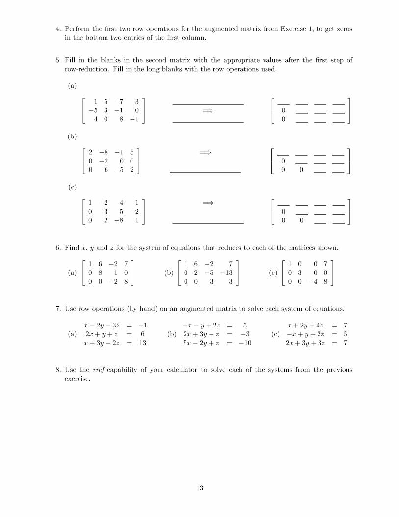
4. Perform the first two row operations for the augmented matrix from Exercise 1, to get zerosin the bottom two entries of the first column.
5. Fill in the blanks in the second matrix with the appropriate values after the first step ofrow-reduction. Fill in the long blanks with the row operations used.
(a)
1 5 −7 3−5 3 −1 04 0 8 −1
=⇒
00
(b)
2 −8 −1 50 −2 0 00 6 −5 2
=⇒
00 0
(c)
1 −2 4 10 3 5 −20 2 −8 1
=⇒
00 0
6. Find x, y and z for the system of equations that reduces to each of the matrices shown.
(a)
1 6 −2 70 8 1 00 0 −2 8
(b)
1 6 −2 70 2 −5 −130 0 3 3
(c)
1 0 0 70 3 0 00 0 −4 8
7. Use row operations (by hand) on an augmented matrix to solve each system of equations.
(a)x− 2y − 3z = −12x+ y + z = 6x+ 3y − 2z = 13
(b)−x− y + 2z = 52x+ 3y − z = −35x− 2y + z = −10
(c)x+ 2y + 4z = 7−x+ y + 2z = 52x+ 3y + 3z = 7
8. Use the rref capability of your calculator to solve each of the systems from the previousexercise.
13

1.4 Applications: Curve Fitting and Temperature Equilibrium
Performance Criterion:
1. (k) Use systems of equations to solve curve fitting and temperature equi-librium problems.
Curve Fitting
Curve fitting refers to the process of finding a polynomial function of “minimal degree” whosegraph contains some given points. We all know that any two distinct points (that is, points thatare not the same) in R
2 have exactly one line through them. In a previous course you should havelearned how to find the equation of that line in the following manner. Suppose that we wish tofind the equation of the line through the points (2, 3) and (6, 1). We know that the equation ofa line looks like y = mx + b, where m and b are to be determined. m is the slope, which can befound by m = 3−1
2−6 = 2−4 = −1
2 . Therefore the equation of our line looks like y = −12x + b.
To find b we simply substitute either of the given ordered pairs into our equation (the fact thatboth pairs lie on the line means that either pair is a solution to the equation) and solve for b:3 = −1
2(2)+b =⇒ b = 4. The equation of the line through (2, 3) and (6, 1) is then y = −12x+4.
We will now solve the same problem in a different way. A student should understand thatwhenever a new approach to a familiar exercise is taken, there is something to be gained byit. Usually the new method is in some way more powerful, and allows the solving of additionalproblems. This will be the case with the following example.
⋄ Example 1.4(a): Find the equation of the line containing the points (2, 3) and (6, 1).
We are again trying to find the two constants m and b of the equation y = mx + b. Herewe substitute the values of x and y from each of the two points into the equation y = mx +b (separately, of course!) to get two equations in the two unknowns m and b. The resultingsystem is then solved for m, then b.
3 = 2m+ b
1 = 6m+ b=⇒ 2m+ b = 3
−6m− b = −1 2(−12 ) + b = 3
−4m = 2 =⇒ −1 + b = 3
m = −12 b = 4
The equation of a line is considered to be a first-degree polynomial, since the power of x iny = mx + b is one. Note that when we have two points in the xy-plane we can find a first-degree polynomial whose graph contains the point. Similarly, when given three points we canfind a second-degree polynomial (quadratic polynomial) whose graph contains the three points. Ingeneral,
Theorem 1.4.1: Given n points in the plane such that (a) no two of themhave the same x-coordinate and (b) they are not collinear, we can find a uniquepolynomial function of degree n− 1 whose graph contains the n points.
14

Often in mathematics we are looking for some object (solution) and we wish to be certain thatsuch an object exists. In addition, it is generally preferable that only one such object exists. Werefer to the first desire as “existence,” and the second is “uniqueness.” If we have, for example,four points meeting the two conditions of the above theorem, there would be infinitely manyfourth degree polynomials whose graphs would contain them, and the same would be true for fifthdegree, sixth degree, and so on. But the theorem guarantees us that there is only one third degreepolynomial whose graph contains the four points.
Now let’s see how we find such a polynomial for degrees higher than two.
⋄ Example 1.4(b): Find the equation of the third degree polynomial containing the points
(−1, 7), (0,−1), (1,−5) and (2, 11).
A general third degree polynomial has an equation of the form y = ax3+bx2+cx+d; our goal isto find values of a, b, c and d so that the given points all satisfy the equation. Since the valuesx = −1, y = 7 must make the general equation true, we have 7 = a(−1)3+b(−1)2+c(−1)+d =−a+ b− c + d. Doing this with all four given ordered pairs and “flipping” each equation givesus the system
−a+ b− c+ d = 7d = −1
a+ b+ c+ d = −58a+ 4b+ 2c+ d = 11
If we enter the augmented matrix for this system in our calculators and rref we get
1 0 0 0 −10 1 0 0 20 0 1 0 −50 0 0 1 −1
So a = −1, b = 2, c = −5, d = −1, and the desired polynomial equation is y = −x3 + 2x2 −5x− 1.
Temperature Equilibrium
Consider the following hypothetical situation: We have a plate of metal that is perfectly insu-lated on both of its faces so that no heat can get in or out of the faces. Each point on the edge,however, is held at a constant temperature (constant at that point, but possibly differing frompoint to point). The temperatures on the edges affect the interior temperatures. If the plate isleft alone for a long time (“infinitely long”), the temperature at each point on the interior of theplate will reach a constant temperature, called the “equilibrium temperature.” This equilibriumtemperature at any given point is a weighted average of the temperatures at all the boundarypoints, with temperatures at closer boundary points being weighted more heavily in the averagethan points that are farther away.
The task of trying to determine those interior temperatures based on the edge temperaturesis one of the most famous problems of mathematics, called the Dirichlet problem (pronounced“dir-i-shlay”). Finding the exact solution involves methods beyond the scope of this course, but wewill use systems of equations to solve the problem “numerically,” which means to approximate theexact solution, usually by some non-calculus method. The key to solving the Dirichlet problem isthe following:
15

Theorem 1.4.2: Mean Value Property
The equilibrium temperature at any interior point P is the average of thetemperatures of all interior points on any circle centered at P .
We will solve what are called discrete versions of the Dirichlet problem, which means that weonly know the temperatures at a finite number of points on the boundary of our metal plate, andwe will only find the equilibrium temperatures at a finite number of the interior points.
⋄ Example 1.4(c): The temperatures (in degrees Fahrenheit) atsix points on the edge of a rectangular plate are shown to the right.Assuming that the plate is insulated as described above and thattemperatures in the plate have reached equilibrium, find the interiortemperatures t1 and t2 at their indicated “mesh points.”
t1
t2
15
15
60
45
45
30
The discrete version of the mean value property tells us that the equi-librium temperature at any interior point of the mesh is the average ofthe four adjacent points. This gives us the two equations
t1 =15 + 45 + 60 + t2
4and t2 =
15 + t1 + 45 + 30
4
If we multiply both sides of each equation by four, combine the constants and get the t1 and
t2 terms on the left side we get the system of equations4t1 − t2 = 120−t1 + 4t2 = 90
, which gives us
t1 = 38 and t2 = 32. These can easily be shown to verify our discrete mean value property:
15 + 45 + 60 + t2
4=
15 + 45 + 60 + 32
4= 38 = t1 ,
15 + t1 + 45 + 30
4=
15 + 38 + 45 + 30
4= 32 = t2
Section 1.4 Exercises
1. Consider the four points (−1, 3), (1, 5), (2, 4) and (4,−1). It turns out that there is aunique third degree polynomial of the form
y = a+ bx+ cx2 + dx3 (1)
whose graph contains those four points. The objective of this exercise is to find the values ofthe coefficients a, b, c and d.
(a) Substitute the x and y values from the first ordered pair into (1) and rearrange theresulting equation so that it has all of the unknowns on the left and a number on theright, like all of the linear equations we have worked with so far.
(b) Repeat (a) for the other 3 ordered pairs, and give the system of equations to be solved.
(c) Give the augmented matrix for the system of equations.
16

(d) Use your calculator or an online tool to rref the augmented matrix. Give the values ofthe unknowns, each rounded to the nearest hundredth, based on the reduced matrix.
(e) Give the equation of the polynomial. Graph it using some technology, and make surethat it appears to go through the points that it is supposed to.
2. (a) Find the equation of the quadratic polynomial y = ax2 + bx + c whose graph is theparabola passing through the points (−1,−4), (1, 1) and (3, 0).
(b) Graph your answer on your calculator and use the trace function to see if the graph infact goes through the three given points.
3. (a) Plot the points (−4, 0), (−2, 2), (0, 0), (2, 2) and (3, 0) neatly on an xy grid. Sketchthe graph of a polynomial function with the fewest number of turning points (“humps”)possible that goes through all the points. What is the degree of the polynomial function?
(b) Find a fourth degree polynomial y = a0 + a1x+ a2x2 + a3x
3 + a4x4 that goes through
the given points.
(c) Graph your function from (b) on your calculator and sketch it, using a dashed line, onyour graph from (a). Is the graph what you expected?
4. The equation of a plane in R3 can always be written in the form z = a + bx+ cy, where a,
b and c are constants and (x, y, z) is any point on the plane. Use a method similar to theabove method for finding the equation of a line to find the equation of the plane through thethree points P1(−5, 0, 2), P2(4, 5,−1) and P3(2, 2, 2). Use your calculator’s rref command tosolve the system. Round a, b and c to the thousandth’s place.
5. Temperatures at points along the edges of a rectangular plate are as shown below and to theleft. Find the equilibrium temperature at each of the interior points, to the nearest tenth.
t1 t2 t3
t4 t5 t6
47
51
66
62
52 58 63
55 57 60
Exercise 5
t1
t2
t3
t4
10
15
20
25
10
15
20
25
5
30Exercise 6
6. Consider the rectangular plate with boundary temperatures shown above and to the right.
(a) Intuitively, what do you think that the equilibrium temperatures t1, t2, t3 and t4 are?
(b) Set up a system of equations and find the equilibrium temperatures. How was yourintuition?
7. For the diagram to the right, the mean value property still holds,even though the plate in this case is triangular. Find the interiorequilibrium temperatures, rounded to the nearest tenth.
60
60
60
40 40 40
20
20
20
t1
t2 t3
17
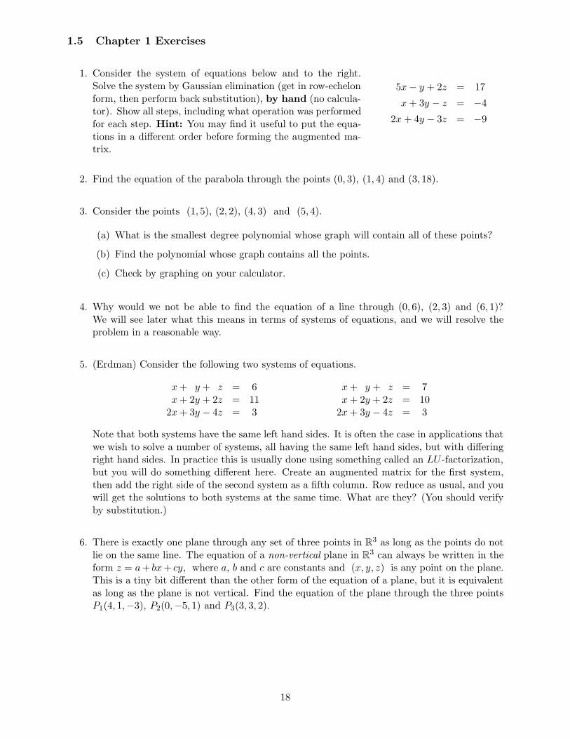
1.5 Chapter 1 Exercises
1. Consider the system of equations below and to the right.Solve the system by Gaussian elimination (get in row-echelonform, then perform back substitution), by hand (no calcula-tor). Show all steps, including what operation was performedfor each step. Hint: You may find it useful to put the equa-tions in a different order before forming the augmented ma-trix.
5x− y + 2z = 17
x+ 3y − z = −42x+ 4y − 3z = −9
2. Find the equation of the parabola through the points (0, 3), (1, 4) and (3, 18).
3. Consider the points (1, 5), (2, 2), (4, 3) and (5, 4).
(a) What is the smallest degree polynomial whose graph will contain all of these points?
(b) Find the polynomial whose graph contains all the points.
(c) Check by graphing on your calculator.
4. Why would we not be able to find the equation of a line through (0, 6), (2, 3) and (6, 1)?We will see later what this means in terms of systems of equations, and we will resolve theproblem in a reasonable way.
5. (Erdman) Consider the following two systems of equations.
x+ y + z = 6x+ 2y + 2z = 112x+ 3y − 4z = 3
x+ y + z = 7x+ 2y + 2z = 10
2x+ 3y − 4z = 3
Note that both systems have the same left hand sides. It is often the case in applications thatwe wish to solve a number of systems, all having the same left hand sides, but with differingright hand sides. In practice this is usually done using something called an LU -factorization,but you will do something different here. Create an augmented matrix for the first system,then add the right side of the second system as a fifth column. Row reduce as usual, and youwill get the solutions to both systems at the same time. What are they? (You should verifyby substitution.)
6. There is exactly one plane through any set of three points in R3 as long as the points do not
lie on the same line. The equation of a non-vertical plane in R3 can always be written in the
form z = a+ bx+ cy, where a, b and c are constants and (x, y, z) is any point on the plane.This is a tiny bit different than the other form of the equation of a plane, but it is equivalentas long as the plane is not vertical. Find the equation of the plane through the three pointsP1(4, 1,−3), P2(0,−5, 1) and P3(3, 3, 2).
18

7. As described in the book, when a plate or solid object reaches atemperature equilibrium, the temperature at any interior point isthe average of the temperatures at all points on any circle or spherecentered at that point and not extending outside the plate or object.Consider the plate of metal shown to the right, with boundary tem-peratures as indicated. The numbers t1, t2, t3 and t4 representthe equilibrium temperatures at the four interior points marked bydots. In the lower picture to the right I have drawn a circle centeredat the point with temperature t1.
(a) Write an equation that gives the temperature t1 as the averageof the four known or unknown temperatures on the circle. Mul-tiply both sides by four to eliminate the fraction, and get all theunknowns on one side and all numbers on the other. You shouldend up with an equation of the form at1 + bt2 + ct3 + dt4 = e,where not all terms will be present on the left side.
(b) Repeat (a) for the other three interior points, averaging thetemperatures on circles of the same size around each.
(c) Solve the resulting system of equations to determine each inte-rior point, rounded to the nearest tenth.
t1 t2
t3 t4
68 65
53 50
61 59
55 52
t1 t2
t3
t4
68 65
53 50
61 59
55 52
8. Given a matrix A, we refer to the values in the matrix as entries, and they are eachrepresented as ajk, where i is the row of the entry, and j is the column of the entry. (Thenumbering for rows and columns begins with one for each, and at the upper left corner.)
(a) Set up systems of equations to solve Section 1.4 Exercises 5, 6, 7. Find the coefficientmatrix in each case, and observe each carefully. You should see two or three things theyall have in common. Use the notation just described for entries of a matrix to helpdescribe what you see. You should be able to summarize your observations injust a couple brief mathematical statements.
(b) Solve each of the exercises listed in part (a). For each sheet, look at where the maximumand minimum temperatures occur.What can we say in general about the locations of themaximum and minimum temperatures? Can you see how this is implied by the MeanValue Property?
9. (a) A student is attempting to find the equilibrium temperatures at points t1, t2, t3 andt4 on a plate with a grid and boundary temperatures shown below and to the left. Theyget t1 = 50.3, t2 = 67.4, t3 = 53.6, t4 = 60.5. Explain in one complete sentence whytheir answer must be incorrect, without finding the solution.
t1 t2
t3 t4
47
51
66
62
52 58
55 57
4 −1 0 0 −1 0 103
−1 4 −1 0 0 −1 92
0 −1 4 −1 −1 0 110
0 0 −1 4 0 0 98
−1 0 −1 0 4 0 105
0 −1 0 0 −1 4 107
19

(b) A different student is trying to solve another such problem, and their augmented matrixis shown above and to the right. How do we know that one of their equations is incorrect,without setting up the equations ourselves?
10. Given a cube of some solid material, it is possible to puta three-dimensional grid into the solid, in the same waythat we put a two-dimensional grid on a rectangular plate.Given temperatures at all nodes on the exterior faces ofthe cube, we can find equilibrium temperatures at eachinterior node using a system of equations. Once again thekey is the mean-value property. In this three dimensionalcase this property tells us that the equilibrium tempera-ture at each interior node is equal to the average of all thetemperatures at nodes of the grid that are immediatelyadjacent to the point in question. To the right I haveshown a cube that has eight interior grid points. Theword “slice” is used here to mean a cross section through
front face slice 1slice 2
back face (behind)
the cube. The grids below show temperatures, known or unknown, at all nodes on the frontface, each of the two slices, and the back face. Above and to the right I have “exploded” thecube to show the temperatures on the front and back faces, and the two slices. Of courseeach node on any slice is connected to the corresponding node on the adjacent slice or face.
37 40
39 41
front face
t11 t12
t13 t14
41 42
40 41
40 43
40 44
slice 1
t21 t22
t23 t24
45 48
43 45
43 50
42 49
slice 2
47 54
49 52
back face
(a) Using the Mean Value Property in three dimensions, the temperature at each interiorpoint will NOT be the average of four temperatures, like it was on a plate. How manytemperatures will be averaged in this case?
(b) Set up a system of equations to solve for the interior temperatures, and find each to thenearest tenth.
11. Do any of your observations from Exercise 8 change in the three dimensional case?
12. Suppose we are solving a system of three equations in the three unknowns x1, x2 and x3,with the unknowns showing up in the equations in that order. It is possible to do row reductionin such a way as to obtain the matrix
1 0 0 53 −2 0 7−1 5 2 −3
Determine x1, x2 and x3 without row-reducing this matrix! you should be able to simplyset up equations and find values for the unknowns.
20

13. Find the currents I1, I2 and I3 in the circuit with the diagram shown below and to theleft.
2 Ω
1Ω 3Ω
4Ω
24 V
30 VI1I1
I3
I2 I2
I3
I3
Exercise 13
3Ω
1Ω 4Ω
1Ω
V2
12VI1I1
I3
I2 I2
I3
I3AB
Exercise 14
14. Consider the circuit with the diagram shown above and to the right.
(a) Find the currents I1, I2 and I3 when the voltage V2 is 6 volts, rounded to the tenth’splace.
(b) Does the current in the middle branch of the circuit flow from A to B, or from B to A?
(c) Find the currents I1, I2 and I3 when the voltage V2 is 24 volts, rounded to thetenth’s place.
(d) Does the current in the middle branch of the circuit flow from A to B, or from B to A?
(e) Determine the voltage needed for V2 in order that no current flows through the middlebranch. (You might wish to row reduce by hand for this...)
21

22
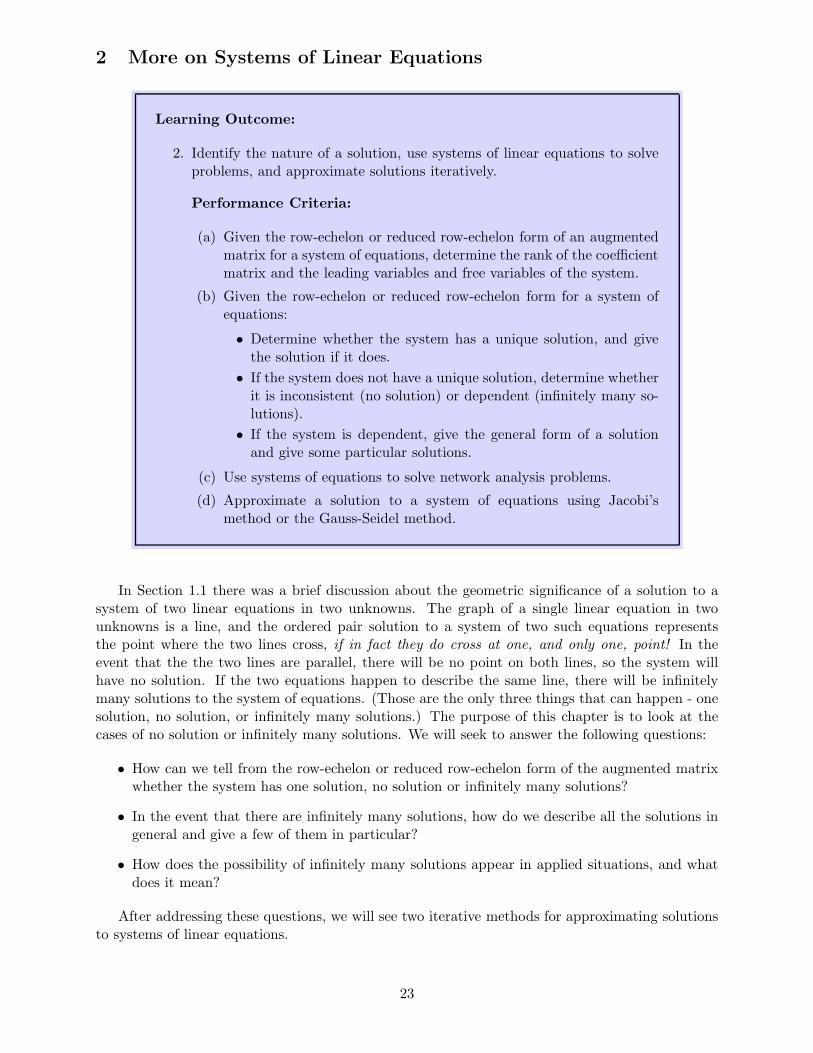
2 More on Systems of Linear Equations
Learning Outcome:
2. Identify the nature of a solution, use systems of linear equations to solveproblems, and approximate solutions iteratively.
Performance Criteria:
(a) Given the row-echelon or reduced row-echelon form of an augmentedmatrix for a system of equations, determine the rank of the coefficientmatrix and the leading variables and free variables of the system.
(b) Given the row-echelon or reduced row-echelon form for a system ofequations:
• Determine whether the system has a unique solution, and givethe solution if it does.
• If the system does not have a unique solution, determine whetherit is inconsistent (no solution) or dependent (infinitely many so-lutions).
• If the system is dependent, give the general form of a solutionand give some particular solutions.
(c) Use systems of equations to solve network analysis problems.
(d) Approximate a solution to a system of equations using Jacobi’smethod or the Gauss-Seidel method.
In Section 1.1 there was a brief discussion about the geometric significance of a solution to asystem of two linear equations in two unknowns. The graph of a single linear equation in twounknowns is a line, and the ordered pair solution to a system of two such equations representsthe point where the two lines cross, if in fact they do cross at one, and only one, point! In theevent that the the two lines are parallel, there will be no point on both lines, so the system willhave no solution. If the two equations happen to describe the same line, there will be infinitelymany solutions to the system of equations. (Those are the only three things that can happen - onesolution, no solution, or infinitely many solutions.) The purpose of this chapter is to look at thecases of no solution or infinitely many solutions. We will seek to answer the following questions:
• How can we tell from the row-echelon or reduced row-echelon form of the augmented matrixwhether the system has one solution, no solution or infinitely many solutions?
• In the event that there are infinitely many solutions, how do we describe all the solutions ingeneral and give a few of them in particular?
• How does the possibility of infinitely many solutions appear in applied situations, and whatdoes it mean?
After addressing these questions, we will see two iterative methods for approximating solutionsto systems of linear equations.
23

2.1 “When Things Go Wrong”
Performance Criteria:
2. (a) Given the row-echelon or reduced row-echelon form of an augmentedmatrix for a system of equations, determine the rank of the coefficientmatrix and the leading variables and free variables of the system.
(b) Given the row-echelon or reduced row-echelon form for a system ofequations:
• Determine whether the system has a unique solution, and givethe solution if it does.
• If the system does not have a unique solution, determine whetherit is inconsistent (no solution) or dependent (infinitely many so-lutions).
• If the system is dependent, give the general form of a solutionand give some particular solutions.
Consider the three systems of equations
x− 3y = 6−2x+ 5y = −5
2x− 5y = 3−4x+ 10y = 1
2x− 5y = 4
−4x+ 10y = −8
For the first system, if we multiply the first equation by 2 and add it to the second, we get −y = 7,so y = −7. This can be substituted into either equation to find x, and the system is solved!
When attempting to solve the second and third equations, things do not “work out” in thesame way. In both cases we would likely attempt to eliminate x by multiplying the first equationby two and adding it to the second. For the second system this results in 0 = 7 and for the thirdthe result is 0 = 0. So what is happening? Let’s keep the unknown value y in both equations:0y = 7 and 0y = 0. There is no value of y that can make 0y = 7 true, so there is no solutionto the second system of equations. We call a system of equations with no solution inconsistent.
The equation 0y = 0 is true for any value of y, so y can be anything in the third system ofequations. Thus we will call y a free variable, meaning it is free to have any value. In this sortof situation we will assign another unknown, usually t, to represent the value of the free variable.If there is another free variable we usually use s and t for the two free variables. Once we haveassigned the value t to y, we can substitute it into the first equation and solve for x to getx = 5
2t+ 2.What all this means is that any ordered pair of the form (52 t+ 2, t) will be a solution to the
third system of equations above. For example, when t = 0 we get the ordered pair (2, 0), whent = −6 we get (−13,−6). You can verify that both of these are solutions, as are infinitely manyother pairs. At this point you might note that we could have made x the free variable, then solvedfor y in terms of whatever variable we assigned to x. It is standard convention, however, to startassigning free variables from the last variable, and you will be expected to follow that convention inthis class. A system like this, with infinitely many solutions, is called a dependent system.
The fundamental fact that should always be kept in mind is this.
24

Solutions to a System of Equations
Every system of linear equations has either
• one unique solution
• no solution (the system is inconsistent)
• infinitely many solutions (the system is dependent)
In the context of both linear algebra and differential equations, mathematicians are alwaysconcerned with “existence and uniqueness.” What this means is that when attempting to solve asystem of equations or a differential equation, one cares about
1) whether at least one solution exists and
2) if there is at least one solution, is there exactly one; that is, is the solution unique?
We’ll now see if we can learn to recognize which of the above three situations is the case, basedon the row-echelon or reduced row-echelon form of the augmented matrix of a system. If the threesystems we have been discussing are put into augmented matrix form and row reduced we get
[
1 0 −150 1 −7
] [
2 −5 30 0 7
] [
2 −5 40 0 0
]
It should be clear that the first matrix gives us the unique solution to that system. The secondline of the second matrix “translates” back to the equation 0x+ 0y = 7, which clearly cannot betrue for any values of x or y. So that system has no solution.
If the row reduced augmented matrix for a system has any row with entries allzeros EXCEPT the last one, the system has no solution. The system is said tobe inconsistent.
We now consider the third row reduced matrix. The last line of it “translates” to 0x+0y = 0,which is true for any values of x and y. That means we are free to choose the value of eitherone but, as discussed before, it is customary to let y be the free variable. So we let y = t andsubstitute that into the equation 2x− 5y = 4 represented by the first line of the reduced matrix.As before, that is solved for x to get x = 5
2 t + 2. The solutions to the system are thenx = 5
2t+ 2, y = t for all values of t.We will now consider the system shown below and to the left; its augmented matrix reduces to
the form shown below and to the right.
x1 − x2 + x3 = 3
2x1 − x2 + 4x3 = 7
3x1 − 5x2 − x3 = 7
1 0 3 40 1 2 10 0 0 0
There is one observation we need to make, and we will develop some terminology that makes iteasier to talk about what is going on. First we note that if we were to perform row-reductionon the coefficient matrix of the equation alone, the result would be the same as the row-reducedaugmented matrix, but without the last column. We now make the following definitions:
25

• The rank of a matrix is the number of non-zero rows in its row-echelon or reduced row-echelonform.
• The leading variables are the variables corresponding to the columns of the reduced matrixcontaining the first non-zero entries (always ones for reduced row-echelon form) in each row.For the above system the leading variables are x1 and x2.
• Any variables that are not leading variables are free variables, so x3 is the free variable inthe above system. This means it is free to take any value.
You already know how to solve a system of equations with a single solution, from its reduced row-echelon matrix. If the last non-zero row of the reduced matrix is all zeros except its last entry, itcorresponds to an equation with no solution, so the system has no solution. If neither of those isthe case, then the system will have infinitely many solutions. It is a bit difficult to explain how tosolve such a system, and it is probably best seen by some examples. However, let me try to describeit. Start with the last variable and solve for it if it is a leading variable. If it is not, assign it aparameter, like t. If the next to last variable is a leading variable solve for it, either as a number orin terms of the parameter assigned to the last variable. Continue in this manner until all variableshave been determined as numbers or in terms of parameters.
⋄ Example 2.1(a): Solve the system
x1 − x2 + x3 = 3
2x1 − x2 + 4x3 = 7
3x1 − 5x2 − x3 = 7
The row-reduced form of the augmented matrix for this system is
1 0 3 40 1 2 10 0 0 0
. In this case
the leading variables are x1 and x2. Any variables that are not leading variables are free variables,so x3 is the free variable in this case. If we let x3 = t, the last non-zero row gives the equationx2 + 2t = 1, so x2 = −2t + 1. The first row gives the equation x1 + 3x3 = 4, sox1 = −3t+ 4 and the final solution to the system is
x1 = −3t+ 4, x2 = −2t+ 1, x3 = t
We can also think of the solution as being any ordered triple of the form (−3t+ 4,−2t+ 1, t).
⋄ Example 2.1(b): A system of three equations in the four variables x1, x2, x3 and x4 givesthe row-reduced matrix
1 0 3 0 −10 1 −5 0 20 0 0 1 4
Give the general solution to the system.
The leading variables are x1, x2 and x4. Any variables that are not leading variables are the freevariables, so x3 is the free variable in this case. We can see that the last row gives us x4 = 4. Ifwe let x3 = t, the second equation from the row-reduced matrix is x2 − 5t = 2, so x2 = 5t + 2.The first equation is x1 + 3t = −1, giving x1 = −3t − 1. The final solution to the system isthen
x1 = −3t− 1, x2 = 5t+ 2, x3 = t, x4 = 4,
or (−3t− 1, 5t + 2, t, 4).
26

The solutions given in the previous two examples are called general solutions, because theytell us what any solution to the system looks like in the cases where there are infinitely manysolutions. We can also produce some specific numbers that are solutions as well, which we willcall particular solutions. These are obtained by simply letting any parameters take on whatevervalues we want.
⋄ Example 2.1(c): Give three particular solutions to the system in Example 2.1(a).
If we take the easiest choice for t, zero, we get the particular solution (4, 1, 0). Letting t equalnegative one and one gives us the particular solutions (7, 3,−1) and (1,−1, 1).
The following examples show a situations in which there are two free variables, and one in whichthere is no solution.
⋄ Example 2.1(d): A system of equations in the four variables x1, x2, x3 and x4 that hasthe row-reduced matrix
1 2 0 −1 20 0 1 −2 30 0 0 0 0
Give the general solution and four particular solutions.
In this case, the rank of the matrix is two, the leading variables are x1 and x3, and the freevariables are x2 and x4. We begin by letting x4 = t; we have the equation x3 − 2t = 3, givingus x3 = 2t+ 3. Since x2 is a free variable, we call it something else. t has already been used, solet’s say x2 = s. The first equation indicated by the row-reduced matrix is then x1 + 2s− t = 2,giving us x1 = −2s+ t+ 2. The solution to the corresponding system is
x1 = −2s+ t+ 2, x2 = s, x3 = 2t+ 3, x4 = t
If we let s = 0 and t = 0 we get the solution (2, 0, 3, 0), and if we let s = 2 and t = −1 we get(−3, 2, 1,−1). Letting s = 0 and t = 1 gives the particular solution (3, 0, 5, 1) and letting s = 1and t = 0 gives the particular solution (0, 1, 3, 0).
The values used for the parameters in Examples 2.1(c) and (d) were chosen arbitrarily; anyvalues can be used for t.
⋄ Example 2.1(e): A system of equations in the four variables x1, x2, x3 and x4 has therow-reduced matrix
1 2 0 −1 20 0 1 −2 30 0 0 0 5
Solve the system.
Since the last row is equivalent to the equation 0x1 + 0x2 + 0x3 + 0x4 = 5, which has nosolution, the system itself has no solution.
27

We conclude this section with a few examples concerning the idea of rank.
⋄ Example 2.1(f): Give the ranks of the coefficient matrices from examples 2.1(a), (b), (d)
and (e).
The row-reduced forms of the coefficient matrices for the systems are
1 0 30 1 20 0 0
1 0 0 30 1 0 −50 0 0 1
1 2 0 −10 0 1 −20 0 0 0
with the last being the row-reduced form of the coefficient matrices for both Example 2.1(d) and2.1(e). The rank of the coefficient matrices for Examples 2.1(a), (e) and (f) are all two, and therank of the coefficient matrix for Example 2.1(b) is three.
Section 2.1 Exercises
1. Consider the system of equations
2x− 4y − z = −44x− 8y − z = −4−3x+ 6y + z = 4
.
(a) Determine which of the following ordered triples are solutions to the system of equations:
(6, 3, 4) (3,−1, 4) (0, 0, 4) (−2,−1, 4) (5, 2, 0) (2, 1, 4)
Look for a pattern in the ordered triples that ARE solutions. Try to guess anothersolution, and test your guess by checking it in all three equations. How did you do?
(b) When you tried to solve the system using your calculator, you should have gotten thereduced echelon matrix as
1 −2 0 00 0 1 40 0 0 0
.
Give the system of equations that this matrix represents. Which variable can you de-termine?
(c) It is not possible to determine y, so we simply let it equal some arbitrary value, whichwe will call t. So at this point, z = 4 and y = t. Substitute these into the first equationand solve for x. Your answer will be in terms of t. Write the ordered triple solution tothe system.
NOTE: The system of equations you obtained in part (b) and solved in part (c) has infinitelymany solutions, but we do know that every one of them has the form (2t, t, 4). Note howthis explains the results of part (b).
2. The reduced echelon form of the matrix for the system
3x− 2y + z = −72x+ y − 4z = 0
x+ y − 3z = 1
is
1 0 −1 −10 1 −2 20 0 0 0
.
28

(a) In this case, z cannot be determined, so we let z = t. Now solve for y, in terms of t.Then solve for x in terms of t.
(b) Pick a specific value for t and substitute it into your general form of a solution triple forthe system. Check it by substituting it into all three equations in the original system.
(c) Repeat (b) for a different value of t.
3. The reduced echelon forms of some systems are given below. Find the solutions for any thathave solutions. (Some may have single solutions, some may have infinitely many solutions,and some may not have solutions.)
(a)
1 0 −1 0 40 1 2 0 −50 0 0 1 3
(b)
1 3 0 0 50 0 1 0 10 0 0 1 −4
(c)
1 −3 0 1 −40 0 1 −2 50 0 0 0 0
(d)
1 0 1 50 1 2 −30 0 0 1
(e)
1 0 −2 1 60 1 3 5 −30 0 0 0 0
(f)
1 0 0 −10 1 0 20 0 1 0
(g)
1 2 −1 10 0 0 00 0 0 0
(h)
1 4 −1 0 −20 0 0 1 70 0 0 0 1
(i)
1 5 0 0 20 0 1 0 10 0 0 1 −40 0 0 0 0
4. Give four particular solutions from the general solution of Example 2.1(b).
5. Below is a system of equations and the reduced row-echelon form of the augmented matrix.Give the leading variables, free variables and the rank of the coefficient matrix.
x + y − 3z = 1
−3x+ 2y − z = 7
2x+ y − 4z = 0
1 0 −1 −10 1 −2 20 0 0 0
6. For the system and reduced row-echelon matrix from the previous exercise, do one of thefollowing:
• If the system has a unique solution, give it. If the system has no solution, say so.
• If the system has infinitely many solutions, give the general solution in terms of param-eters s, t, etc., then give two particular solutions.
Then do the same for the systems whose augmented matrices row reduce to the forms shownbelow.
1 1 −10 0 20 0 0
1 2 −1 0 50 0 0 1 −40 0 0 0 0
29

2.2 Overdetermined and Underdetermined Systems
OK, let’s talk about scientific and engineering reality for a bit. Systems of equations generallyarise in situations where a number of variables are related in ways described by systems of linearequations. Those equations are generally based on measurements (data). In practice, it often is thecase that there is a great deal of data, and we get more equations than unknowns. Usually whenthere are more equations than unknowns the system is inconsistent - there is no solution. This isno good! Systems like this are sometimes said to be overdetermined. This wording relates to thefact that in these situations there is too much information to determine a solution to the system.
You might think “Well, why not just use less data, so that the resulting system has a solution?”Well the additional data gives us some redundancy that can give us better results if we know howto deal with it. The way out of this problem is a method called least-squares, which you’ll dolater. It is a method for dealing with systems that don’t have solutions. What it allows us to dois obtain values that are in some sense the “closest” values there are to an actual solution. Again,more on this later.
When there are fewer equations than unknowns there will be no hope of a unique solution -there will either be no solution or infinitely many solutions. Usually there will be infinitely manysolutions and we call such a system underdetermined, meaning there is not enough information(data) to determine a unique solution.
In the next section we’ll look at an application leading to an underdetermined system, andwe’ll “solve” such systems in the best sense possible, meaning our solutions will depend on someparameter that can take any value.
30

2.3 Application: Network Analysis
Performance Criterion:
2. (c) Use systems of equations to solve network analysis problems.
A network is a set of junctions, which we’ll call nodes, connected by what could be calledpipes, or wires, but which we’ll call directed edges. The word “directed” is used to mean thatwe’ll assign a direction of flow to each edge. (In some cases we might then find the flow to benegative, meaning that it actually flows in the direction opposite from what we have designated asthe direction of flow.) There will also be directed edges coming into or leaving the network. It isprobably easiest to just think of a network of plumbing, with water coming in at perhaps severalplaces, and leaving at several others. However, a network could also model goods moving betweencities or countries, traffic flow in a city or on a highway system, and various other things.
Our study of networks will be based on one simple idea, known as conservation of flow:
At each node of a network, the flow into the node must equal the flow out.
⋄ Example 2.3(a): A one-node network is shown to the right. Findthe unknown flow f .
The flow in is 20 + f and the flow out is 45 + 30, so we have
20 + f = 45 + 30.
Solving, we find that f = 55.
f
3045
20
⋄ Example 2.3(b): Another one-node network is shown to the right.Find the unknown flow f .
The flow in is 70 + f and the flow out is 15 + 30, so we have
70 + f = 15 + 30.
Solving, we find that f = −25, so the flow at the arrow labeled f isactually in the direction opposite to the arrow.
f
3015
70
There is nothing wrong with what we just saw in the last example. When setting up a network wemust commit to a direction of flow for any edges in which the flow is unknown, but when solvingthe system we may find that the flow is in the opposite direction from the way the edge was directedinitially. We may also have less information than we did in the previous two examples, as shownby the next example.
31

⋄ Example 2.3(c): For the one-node network is shown to the right,find the unknown flow f1 in terms of the flow f2.
By conservation of flow,
50 + f2 = f1 + 35.
Solving for f1 gives us f1 = f2+15. Thus if f2 was 10, f1 wouldbe 25 (look at the diagram and think about that), if f2 was 45,f1 would be 60, and so on.
f2
35f1
50
The above example represents, in an applied setting, the idea of a free variable. In this exampleeither variable can be taken as free, but if we know the value of one of them, we’ll “automatically”know the value of the other. The way I worded the example, we were taking f2 to be the freevariable, with the value of f1 then depending on the value of f2.
The systems in these first three examples have been very simple; let’s now look at a morecomplex system.
⋄ Example 2.3(d): Determine the flows f1, f2, f3 andf4 in the network shown below and to the right.
Utilizing conservation of flow at each node, we get the equations
30 + 15 = f1 + f2, 70 + f2 = f3,
f1 = 40 + f4, f3 + f4 = 20 + 55
Rearranging these give us the system of equations shown belowand to the left. The augmented matrix for this system reducesto the matrix shown below and to the right.
f1
f2f3
f4
30
15
70
40
55
20
f1 + f2 = 45f2 − f3 = −70
f1 − f4 = 40f3 + f4 = 75
1 0 0 −1 400 1 0 1 50 0 1 1 750 0 0 0 0
From this we can see that f4 is a free variable, so lets say it has value t. The solution to thenetwork is then
f1 = 40 + t, f2 = 5− t, f3 = 75 − t, f4 = t,
where t is the flow f4.
Let’s think a bit more about this last example. Suppose that f4 = t = 0. The equations givenas the solution to the network then give us f1 = 40, f2 = 5, f3 = 75. We can see this withouteven solving the system of equations. Looking at the node in the lower right, if f4 = 0 one caneasily see that f3 must be 75 in order for the flow in to equal the flow out. Knowing f3, wecan go to the node in the lower left and see that f2 = 5. Finally, f2 = 5 gives is f1 = 40, fromthe node in the upper left. This reasoning is essentially the process of back-substitution!
32

2.4 Approximating Solutions With Iterative Methods
Performance Criterion:
2. (d) Approximate a solution to a system of equations using Jacobi’smethod or the Gauss-Seidel method.
Consider again the rectangular metal plate of Example 1.3(b), asshown to the right, with boundary temperatures specified at a fewpoints. Remember that our goal was to find the temperatures t1 andt2 at the two interior points. Applying the mean-value property wearrived at the equations
t1 =15 + 45 + 60 + t2
4=
120 + t2
4,
t2 =15 + t1 + 45 + 30
4=
90 + t1
4
(1)
t1
t2
15
15
60
45
45
30
In Example 1.4(c) we rearranged these equations and solved the system of two equations in twounknowns by row-reduction. Now we will use what is called an iterative method to approximatethe solution to this problem. An iterative method is one in which successive approximations to asolution are generated in sequence, with each approximation getting closer to the true solution.
The method we’ll use first is called the Jacobi method. Although it is more laborious thansimply solving the system by row reduction in this case, and does not even produce an exactsolution, iterative methods like the Jacobi method are at times preferable to direct methods likerow-reduction. For very large systems the Jacobi method can be less computationally costly thanrow reduction. This is especially true for matrices with lots of zeros, as many that arise in practiceare.
The general idea behind the Jacobi method is to begin by guessing values for both t1 and t2.We’ll denote these first two values by t1(0) and t2(0). The guessed value t2(0) is inserted intothe first equation above for t2, and the guessed value t1(0) is inserted into the second equationfor t1. This allows us to compute new values of t1 and t2, denoted by t1(1) and t2(1). Thesenew values are then inserted into the equations (1) for t1 and t2, as was done with the firstguesses. This process is repeated over and over, resulting in new values for t1 and t2 each time.These values will eventually approach the exact solution values of t1 and t2. Let’s do it!
⋄ Example 2.4(a): Use the Jacobi method to find the third approximations t1(3) and
t2(3) to the above problem.
To begin we need guesses for t1(0) and t2(0). We can guess any values we want, and peoplesometimes use zero for initial guesses. A better guess would be something between the lowestand highest boundary temperatures, so lets use the average of those two, 37.5, for our guesses forboth t1(0) and t2(0). Putting each of those into the equations (1) in order to find t1(1) andt2(1), we get
t1(1) =120 + t2(0)
4=
120 + 37.5
4= 39.375
33

and
t2(1) =90 + t1(0)
4=
90 + 37.5
4= 31.875
We then take each of these new values for t1 and t2 and put them into equations (1) again:
t1(2) =120 + t2(1)
4=
120 + 31.875
4= 37.96875
and
t2(2) =90 + t1(1)
4=
90 + 39.375
4= 32.34375
And once more:
t1(3) =120 + t2(2)
4=
120 + 32.34375
4= 38.0859375
and
t2(3) =90 + t1(2)
4=
90 + 37.96875
4= 31.9921875
In Example 1.3(b) we found that the exact solution to this problem is t1 = 38 and t2 = 32, soafter only three iterations the Jacobi method has given approximations for t1 and t2 that arevery close to the exact solution.
Now we will illustrate another iterative method for approximating solutions, called the Gauss-Seidel method. Note that in the Jacobi method we guessed initial values for both t1 and t2,then used those to find the first approximations of both at the same time. In the Gauss-Seidelmethod we guess a value for just one of t1 or t2 and put it into one of the equations (1) to find theother. Say, for example, we guess initially that t2(0) = 37.5. We put this into the first equation (1)to obtain a first value for t1, which we’ll denote by t1(1), the first approximation for t1. (Wecould just as well have called this t1(0).) This value is then used in the second equation to obtainthe first approximation t2(1) for t2. That value is then put back into the first equation to obtaina second approximation for t1, and so on.
⋄ Example 2.4(b): Use the Gauss-Seidel method to find the third approximations t1(3) and
t2(3) to the system of equations
t1 =120 + t2
4, t2 =
90 + t1
4(1)
We begin with the guess t2(0) = 37.5, and put that into the first of the above equations to findt1(1):
t1(1) =120 + t2(0)
4=
120 + 37.5
4= 39.375
This value is then used in the second equation above to find t2(1):
t2(1) =90 + t1(1)
4=
90 + 39.375
4= 32.34375
We now find t1(2)
t1(2) =120 + t2(1)
4=
120 + 32.34375
4= 38.0859375
34

which, in turn, is used to find t2(2):
t2(2) =90 + t1(2)
4=
90 + 38.0859375
4= 32.02148438
Continuing, we have
t1(3) =120 + t2(2)
4=
120 + 32.02148438
4= 38.00537109
and
t2(3) =90 + t1(3)
4=
90 + 38.00537109
4= 32.00134277
As with the Jacobi method, the Gauss-Seidel method has given us a solution that is very close tothe exact solution.
Section 2.4 Exercises
1. Consider the system
5x− 2y + z = −102x+ 3y − z = −3−x− y + 2z = 5
of equations. This exercise will lead you
through solving the system using the Jacobi method.
(a) Solve the system using row-reduction on your calculator or MATLAB.
(b) Solve the first equation for x, the second for y and the third for z.
(c) Create a table like the one below, or just use the one provided here. Note that thereis an index n that goes from zero to eight, and could go on farther if we wished.Our objective is to create a sequence x(0), x(1), x(2), ... of x values, and similarly fory and z, such that the values converge to the solution to the system. Begin by lettingx(0) = y(0) = z(0) = 0, filling in the table accordingly.
n: 0 1 2 3 4 5 6 7 8
x(n):
y(n):
z(n):
(d) Find x(1) by substituting the values of y(0) and z(0) into your equation from (b)that was solved for x. You should get x(1) = −2; put that value into the correct spoton the table. Then substitute x(0) and z(0) into your second equation from (b), theone where you solved for y. This will give you y(1). Then do the same to get z(1).You now have the first iteration values for x , y and z.
(e) Use your values of x, y and z after the first iteration to find the second iteration values,rounded to two places past the decimal, and place them in the appropriate column.
(f) Repeat this process, using the first iteration values to find the second iteration values
(g) Use Excel to create and finish the table. By the time you reach the eight iteration,your values should be very close to the actual solution. You have just used the Jacobimethod to approximate a solution to the system of equations.
35

2. For this exercise you will again work with the system from the previous exercise, but thistime you will the Gauss-Seidel method to approximate the solution to the system.
(a) On the same Excel worksheet, but farther down, make another table like the one above.Leave x(0) blank and let y(0) = z(0) = 0. Find x(1) in the same way you did before.To find y(1) we want to use the “most recent” values of x and z, so use x(1) andz(0). Then, to find z(1) you will use the most recent values of x and y, which arex(1) and y(1).
(b) You can now copy the column with the n = 1 formulas across the table. Compare theresults with the table for the Jacobi method.
3. For this exercise you’ll be working with the system
x+ 2y + 4z = 7
−x+ y + 2z = 5
2x+ 3y + 3z = 7
.
(a) Use row-reduction to solve the system.
(b) Using the Jacobi method with x(0) = y(0) = z(0) = 0 to find x(1), y(1), z(1) andx(2), y(2), z(2). Do the values obtained appear to be approaching the solution?
36
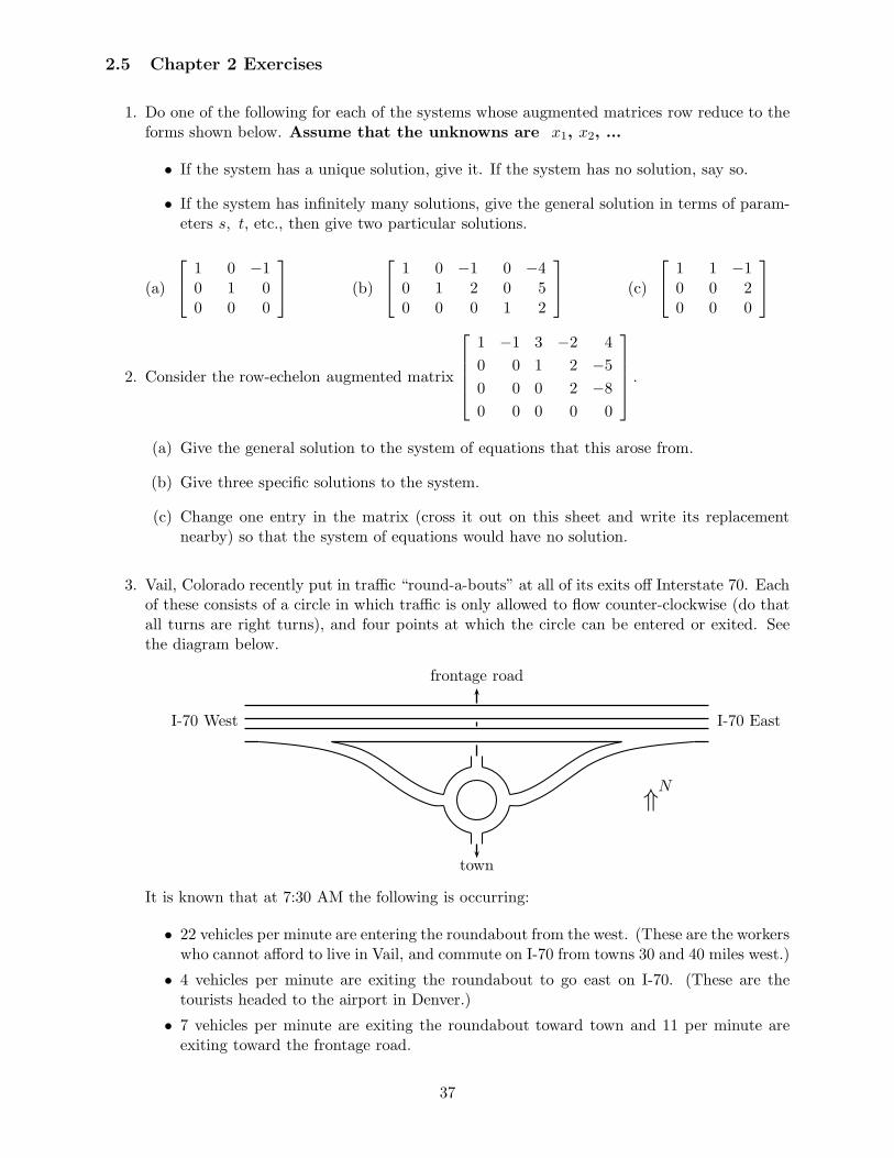
2.5 Chapter 2 Exercises
1. Do one of the following for each of the systems whose augmented matrices row reduce to theforms shown below. Assume that the unknowns are x1, x2, ...
• If the system has a unique solution, give it. If the system has no solution, say so.
• If the system has infinitely many solutions, give the general solution in terms of param-eters s, t, etc., then give two particular solutions.
(a)
1 0 −10 1 00 0 0
(b)
1 0 −1 0 −40 1 2 0 50 0 0 1 2
(c)
1 1 −10 0 20 0 0
2. Consider the row-echelon augmented matrix
1 −1 3 −2 4
0 0 1 2 −50 0 0 2 −80 0 0 0 0
.
(a) Give the general solution to the system of equations that this arose from.
(b) Give three specific solutions to the system.
(c) Change one entry in the matrix (cross it out on this sheet and write its replacementnearby) so that the system of equations would have no solution.
3. Vail, Colorado recently put in traffic “round-a-bouts” at all of its exits off Interstate 70. Eachof these consists of a circle in which traffic is only allowed to flow counter-clockwise (do thatall turns are right turns), and four points at which the circle can be entered or exited. Seethe diagram below.
town
frontage road
I-70 EastI-70 West
N⇑
It is known that at 7:30 AM the following is occurring:
• 22 vehicles per minute are entering the roundabout from the west. (These are the workerswho cannot afford to live in Vail, and commute on I-70 from towns 30 and 40 miles west.)
• 4 vehicles per minute are exiting the roundabout to go east on I-70. (These are thetourists headed to the airport in Denver.)
• 7 vehicles per minute are exiting the roundabout toward town and 11 per minute areexiting toward the frontage road.
37
Solve the system and answer the following:
(a) What is the minimum number of cars per minute passing through the southeast quarterof the roundabout?
(b) If 18 vehicles per minute are passing through the southeast (SE) quarter of the round-about per minute, how many are passing through each of the other quarters (NW, NE,SW)?
4. Consider the system
x1 − x2 − 4x3 = 6
5x1 + x2 − 2x3 = 18
2x1 + 4x2 + 10x3 = 0
.
(a) Use your calculator or an online tool to reduce the matrix to reduced row echelon form.Write the system of two equations represented by the first two rows of the reducedmatrix. (The last equation is of no use, so don’t bother writing it.)
(b) The second equation contains x2 and x3. Suppose that x3 = 1 and compute x2 usingthat equation. Then use the values you have for x2 and x3 in the first equation tofind x1.
(c) Verify that the values you obtained in (b) are in fact a solution to the original systemgiven.
(d) Now let x3 = 0 and repeat the process from (b) to obtain another solution. Verify thatsolution as well.
(e) Let x3 = 2 to find yet another solution.
(f) Because there is no equation allowing us to determine x3, we say that it is a freevariable. What we will usually do in situations like this is let x3 equal some parameter(number) that we will denote by t. That is, we set x3 = t, which is really just renamingit. Substitute t into the second equation from (a) and solve for x2 in terms of t.Then substitute that result into the first equation for x2, along with t for x3, andsolve for x1 in terms of t. Summarize by giving each of x1, x2 and x3 in terms oft, all in one place.
(g) Substitute the number one for t into your answer to (f) and check to see that it matcheswhat you got for (b). If doesn’t, you’ve gone wrong somewhere - find the error and fixit.
5. Solve each of the following systems of equations that have solutions. Do/show the followingthings:
• Enter the augmented matrix for the system in your calculator.
• Get the row-reduced echelon form of the matrix using the rref command. Write downthe resulting matrix.
• Write the system of equations that is equivalent to the row-reduced echelon matrix.
• Find the solutions, if there are any. Use the letters that were used in the original systemfor the unknowns! For those with multiple solutions, give them in terms of a parametert or, when necessary, two parameters s and t.
38

(a)
x1 − x2 + 3x3 = −4−2x1 + 3x2 − 8x3 = 13
5x1 − 3x2 + 11x3 = −10(b)
c1 + 3c2 + 5c3 = 3
2c1 + 7c2 + 9c3 = 5
2c1 + 6c2 + 11c3 = 7
(c)
x1 + 3x2 − 2x3 = −1−7x1 − 21x2 + 14x3 = 7
2x1 + 6x2 − 4x3 = −2(d)
c1 − c2 + 3c3 = −4−2c1 + 3c2 − 8c3 = 13
5c1 − 3c2 + 11c3 = 4
(e)
x− 3y + 7z = 4
5x− 14y + 42z = 29
−2x+ 5y − 20z = −16(f)
x+ 3y = 2
4x+ 12y + z = 1
−x− 3y − 2z = 12
• Give three specific solutions to the system from part (a) above.
• Give three specific solutions to the system from part (c) above.
• Solve the system from part (b) above by hand, showing all steps of the row reductionand indicating what you did at each step.
6. Give the reduced row echelon form of an augmented matrix for a system of four equations infour unknowns x1, x2, x3 and x4 for which
• x4 = 7
• x2 and only x2, is a free variable
7. (Erdman) Consider the systemx+ ky = 1
kx+ y = 1, where k is some constant.
(a) Set up the augmented matrix and use a row operation to get a zero in the lower leftcorner.
(b) For what value or values of k would the system have infinitely many solutions? Whatis the form of the general solution?
(c) For what value or values of k would the system have no solution?
(d) For all remaining values of k the system has a unique solution (that depends on thechoice of k). What is the solution in that case? Your answer will contain the parameterk.
8. (Erdman) Consider the systemx− y − 3z = 3
2x+ z = 02y + 7z = c
, where c is some constant.
(a) Set up the augmented matrix and use a row operation to get a zero in the first entry ofthe second row.
(b) Look at the second and third rows. For what value or values of c can the system besolved? Give the solution if there is a unique solution. Give the general solution if thereare infinitely many solutions.
39

f1f2
f3 f4
8
18
f5
f6
9. The network to the right represents a traffic circle. The num-bers next to each of the paths leading into or out of the circleare the net flows in the directions of the arrows, in vehiclesper minute, during the first part of lunch hour.
(a) Suppose that f3 = 7 and f5 = 4. You should be ableto work your way around the circle, eventually figuringout what each flow is. Do this.
(b) Still assuming that f3 = 7 and f5 = 4, set up anequation at each junction of the circle, to get four equa-tions in four unknowns. Solve the system. What do younotice about your answers?
(c) Now assume that the only flows you know are the ones shown in the diagram. Whenyou set up a system of equations, based on the flows in and out of each junction, howmany equations will you have? How many unknowns? How many free variables do youexpect?
(d) Go ahead and set up the system of equations. Give the augmented matrix and thereduced matrix (obtained with your calculator), and then give the general solution tothe system. Were you correct in how many free variables there are?
(e) Choose the value(s) of the parameter(s) that make f3 = 7 and f5 = 4, then find theresulting particular solution. What do you notice?
(f) What restriction(s) is(are) there on the parameter(s), in order that all flows go in thedirections indicated. (Allow a flow of zero for each flow as well.)
10. For another traffic circle, a student uses the diagram shownbelow and to the right and obtains the flows given below andto the left, in vehicles per minute.
f1 = t− 8, f2 = t+ 3, f3 = t− 5, f4 = t
(a) Determine the minimum value of t that makes eachof f1 through f4 zero or greater. Give the minimumallowable values for each flow, in the form fi ≥ a, as-suming that no vehicles ever go the wrong way arounda portion of the circle. Remember that setting a valuefor any flow determines all the other flows. You mayneglect units.
f1f2
f3 f4
fa
fb
fc
fd
(b) Give each of the flows f1 through f4 when the flow in the northeast quarter (f1) is12 vehicles per minute. You may neglect units.
(c) Determine each of the flows fa through fd, still for f1 = 12. You should be able todo this based only on the four equations given. At least one of them will be negative,indicating that the corresponding arrow(s) should be reversed.
40

11. In a previous exercise, you may have attempted to find the equation of a parabola throughthe three points (−1,−6), (0,−4) and (1,−1). You set up a system to find values of a, b andc in the parabola equation y = ax2+ bx+ c. There was a unique solution, meaning that thereis only one parabola containing those three points. Expect the following to not work out as“neatly.”
(a) Use a system of equations to find the equation of a parabola that goes through just thetwo points (−1,−6) and (1,−1). Explain your results.
(b) Use a system of equations to find the equation y = mx + b of a line through the fourpoints (1.3, 1.5), (0.8, 0.4), (2.6, 3.0) and (2.0, 2.0).
(c) Plot the four points from (b) on a neat and accurate graph, and use what you see toexplain your answer to (b). You should be able to give your explanation in oneor two complete sentences.
12. The diagram to the right shows boundary temperatures for a triangu-lar piece of metal, and a grid connecting some interior points with theboundary. In this exercise you will use the Jacobi Method to approxi-mate the interior temperatures t1, t2 and t3. You will see that aniterative method like the Jacobi method or Gauss-Seidel method workwell for this sort of problem.
(a) Write an equation for each of t1, t2 and t3 as an average ofthe four surrounding temperatures. Combine any numbers that areadded, and notice that you now have three equations in the correctform for an iterative method.
87
82
75
75 77 78
78
83
86
t1
t2 t3
(b) You will now use the Jacobi method to approximate values for t1, t2 and t3, butyou need starting values t1(0), t2(0) and t3(0). You could use just about anything,but the method will converge more quickly if a good choice of initial values is made. Ifyou look at the boundary values, you can see that the average of all of them should bearound 80. (We could find the exact average, but it wouldn’t result in any quickerconvergence.) So use t1(0) = t2(0) = t3(0) = 80 and approximate the values of t1(1),t2(1), t3(1) and t1(2), t2(2), t3(2), rounding to four places past the decimalwhen rounding is necessary.
(c) Repeat part (b), but using the Gauss-Seidel method.
41

42

3 Euclidean Space and Vectors
Outcome:
3. Understand vectors and their algebra and geometry in Rn.
Performance Criteria:
(a) Recognize the equation of a plane in R3 and determine where the
plane intersects each of the three axes. Give the equation of anyone of the three coordinate planes or any plane parallel to one of thecoordinate planes.
(b) Find the distance between two points in Rn.
(c) Find the vector from one point to another in Rn. Find the length
of a vector in Rn.
(d) Multiply vectors by scalars and add vectors, algebraically. Find linearcombinations of vectors algebraically.
(e) Illustrate the parallelogram method and tip-to-tail method for findinga linear combination of two vectors.
(f) Find a linear combination of vectors equalling a given vector.
(g) Find the dot product of two vectors, determine the length of a singlevector.
(h) Determine whether two vectors are orthogonal (perpendicular).
(i) Find the projection of one vector onto another, graphically or alge-braically.
In the study of linear algebra we will be defining new concepts and developing correspondingnotation. The purpose of doing so is to develop more powerful machinery for investigating theconcepts of interest. We begin the development of notation with the following. The set of all realnumbers is denoted by R, and the set of all ordered pairs of real numbers is R
2, spoken as“R-two.” Geometrically, R
2 is the familiar Cartesian coordinate plane. Similarly, the set of allordered triples of real numbers is the three-dimensional space referred to as R
3, “R-three.” Theset of all ordered n-tuples (lists of n real numbers in a particular order) is denoted by R
n.Although difficult or impossible to visualize physically, R
n can be thought of as n-dimensionalspace. All of the R
ns are what are called Euclidean space.
43
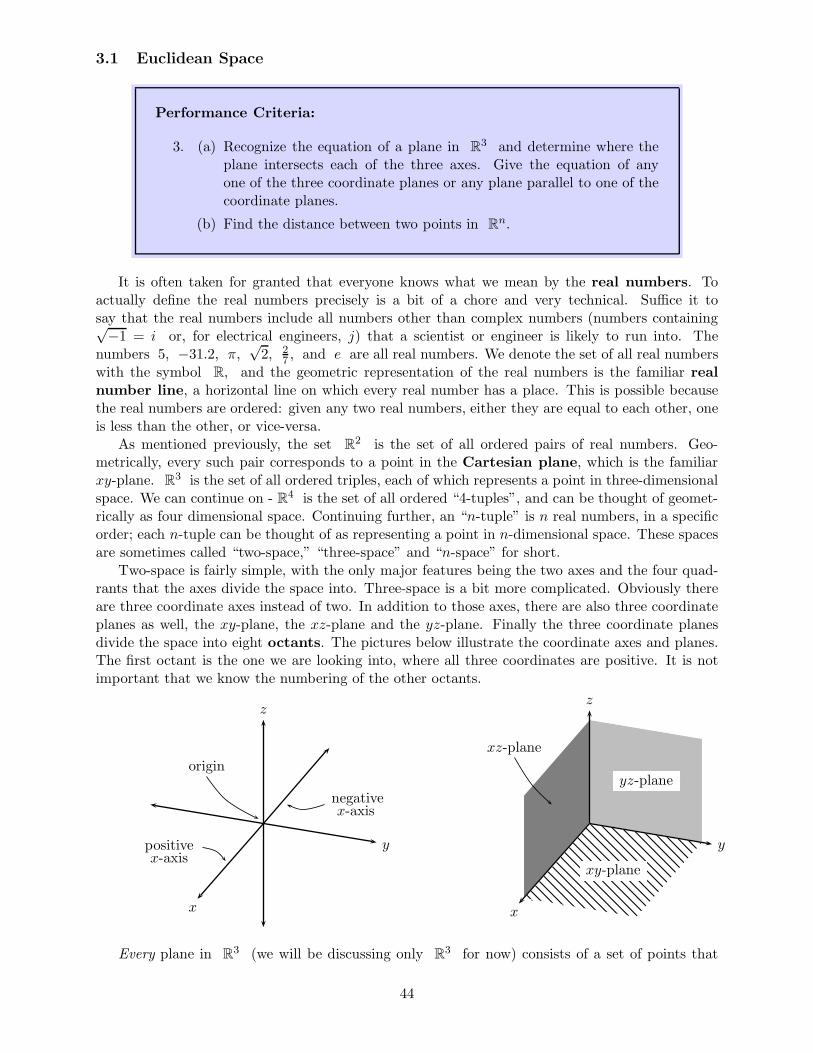
3.1 Euclidean Space
Performance Criteria:
3. (a) Recognize the equation of a plane in R3 and determine where the
plane intersects each of the three axes. Give the equation of anyone of the three coordinate planes or any plane parallel to one of thecoordinate planes.
(b) Find the distance between two points in Rn.
It is often taken for granted that everyone knows what we mean by the real numbers. Toactually define the real numbers precisely is a bit of a chore and very technical. Suffice it tosay that the real numbers include all numbers other than complex numbers (numbers containing√−1 = i or, for electrical engineers, j) that a scientist or engineer is likely to run into. The
numbers 5, −31.2, π,√2, 2
7 , and e are all real numbers. We denote the set of all real numberswith the symbol R, and the geometric representation of the real numbers is the familiar realnumber line, a horizontal line on which every real number has a place. This is possible becausethe real numbers are ordered: given any two real numbers, either they are equal to each other, oneis less than the other, or vice-versa.
As mentioned previously, the set R2 is the set of all ordered pairs of real numbers. Geo-
metrically, every such pair corresponds to a point in the Cartesian plane, which is the familiarxy-plane. R
3 is the set of all ordered triples, each of which represents a point in three-dimensionalspace. We can continue on - R4 is the set of all ordered “4-tuples”, and can be thought of geomet-rically as four dimensional space. Continuing further, an “n-tuple” is n real numbers, in a specificorder; each n-tuple can be thought of as representing a point in n-dimensional space. These spacesare sometimes called “two-space,” “three-space” and “n-space” for short.
Two-space is fairly simple, with the only major features being the two axes and the four quad-rants that the axes divide the space into. Three-space is a bit more complicated. Obviously thereare three coordinate axes instead of two. In addition to those axes, there are also three coordinateplanes as well, the xy-plane, the xz-plane and the yz-plane. Finally the three coordinate planesdivide the space into eight octants. The pictures below illustrate the coordinate axes and planes.The first octant is the one we are looking into, where all three coordinates are positive. It is notimportant that we know the numbering of the other octants.
x
y
z
origin
positivex-axis
negativex-axis
x
y
z
xy-plane
yz-plane
xz-plane
Every plane in R3 (we will be discussing only R
3 for now) consists of a set of points that
44

behave in an orderly mathematical manner, described here:
Equation of a Plane in R3: The ordered triples corresponding to all the
points in a plane satisfy an equation of the form
ax+ by + cz = d,
where a, b, c and d are constants, and not all of a, b and c are zero.
The xy-plane is the plane containing the x and y-axes. The only condition on points in that planeis that z = 0, so that is the equation of that plane. (Here the constants a, b and d are all zero, andc = 1.) The plane z = 5 is a horizontal plane that is five units above the xy-plane.
⋄ Example 3.1(a): Graph the equation 2x + 3y = 6 in the first octant. Indicate clearlywhere it intersects each of the coordinate axes, if it does.
Some points that satisfy the equation are (3, 0, 0), (6,−2, 5), and so on. Since z is notincluded in the equation, there are no restrictions on z; it can take any value. If we were tofix z at zero and plot all points that satisfy the equation, we would get a line in the xy-planethrough the two points (3, 0, 0) and (0, 2, 0). These points are obtained by first letting y andz be zero, then by letting x and z be zero. Since z can be anything, the set of pointssatisfying 2x + 3y = 6 is a vertical plane intersecting the xy-plane in that line. The plane isshown below and to the left.
x
y
z
34
2 3 4
Example 3.1(a) x
y
z
6
34
2 3 4
Example 3.1(b)
⋄ Example 3.1(b): Graph the equation 2x+3y+z = 6 in the first octant. Indicate clearlywhere it intersects each of the coordinate axes, if it does.
The set of points satisfying this equation is also a plane, but z is no longer free to take any value.The simplest way to “get a handle on” such a plane is to find where it intercepts the three axes.Note that every point on the x-axis has y- and z-coordinates of zero. So to find where the planeintersects the x-axis we put zero into the equation for y and z, then solve for x, getting x = 3.The plane then intersects the x-axis at (3, 0, 0). A similar process gives us that the plane intersects
45

the y and z axes at (0, 2, 0) and (0, 0, 6). The graph of the plane is shown in the drawing aboveand to the right.
Consider now a system of equations like
x+ 3y − 2z = −43x+ 7y + z = 4
−2x+ y + 7z = 7
,
which has solution (3,−1, 2). Each of the three equations represents a plane in R3, and the point
(3,−1, 2) is where the three planes intersect. This is completely analogous to the interpretation ofthe solution of a system of two linear equations in two unknowns as the point where the two linesrepresenting the equations cross. This is the first of three interpretations we’ll have for the solutionto a system of equations.
The only other basic geometric fact we need about three-space is this:
Distance Between Points: The distance between two points (x1, y1, z1) and(x2, y2, z2) in R
n is given by
d =√
(x1 − x2)2 + (y1 − y2)2 + (z1 − z2)2
This is simply a three-dimensional version of the Pythagorean Theorem. This is in fact used ineven higher dimensional spaces; even though we cannot visualize the distance geometrically, thisidea is both mathematically valid and useful.
⋄ Example 3.1(c): Find the distance in R3 between the points (−4, 7, 1) and (13, 0,−6).
Using the above formula we get
d =√
(−4− 13)2 + (7− 0)2 + (1− (−6))2 =√
(−17)2 + 72 + 72 =√387 ≈ 19.7
We will now move on to our main tool for working in Euclidean space, vectors.
Section 3.1 Exercises
1. Determine whether each of the equations given describes a plane in R3. If not, say so. If it
does describe a plane, give the points where it intersects each axis. If it doesn’t intersect anaxis, say so.
(a) −2x− y + 3z = −6 (b) x+ 3z = 6 (c) y = −6
(d) x+ 3z2 = 12 (e) x− 2y + 3z = −6
2. Give the equation of a plane in R3 that does not intersect the y-axis but does intersect the
other two axes. Give the points at which it intersects the x- and z-axes.
3. Give the equation of the plane that intersects the y-axis at 4 and does not intersect eitherof the other two axes.
46
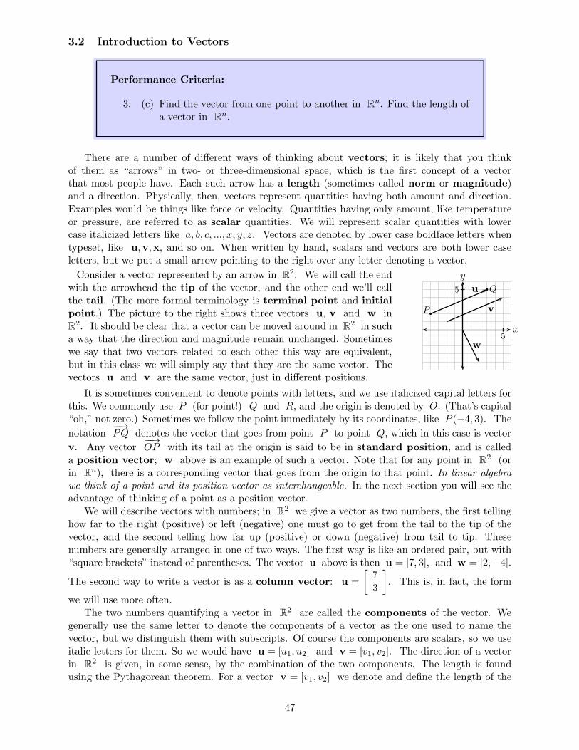
3.2 Introduction to Vectors
Performance Criteria:
3. (c) Find the vector from one point to another in Rn. Find the length of
a vector in Rn.
There are a number of different ways of thinking about vectors; it is likely that you thinkof them as “arrows” in two- or three-dimensional space, which is the first concept of a vectorthat most people have. Each such arrow has a length (sometimes called norm or magnitude)and a direction. Physically, then, vectors represent quantities having both amount and direction.Examples would be things like force or velocity. Quantities having only amount, like temperatureor pressure, are referred to as scalar quantities. We will represent scalar quantities with lowercase italicized letters like a, b, c, ..., x, y, z. Vectors are denoted by lower case boldface letters whentypeset, like u,v,x, and so on. When written by hand, scalars and vectors are both lower caseletters, but we put a small arrow pointing to the right over any letter denoting a vector.
Consider a vector represented by an arrow in R2. We will call the end
with the arrowhead the tip of the vector, and the other end we’ll callthe tail. (The more formal terminology is terminal point and initialpoint.) The picture to the right shows three vectors u, v and w inR2. It should be clear that a vector can be moved around in R
2 in sucha way that the direction and magnitude remain unchanged. Sometimeswe say that two vectors related to each other this way are equivalent,but in this class we will simply say that they are the same vector. Thevectors u and v are the same vector, just in different positions.
5
5
u
v
w
P
Q
x
y
It is sometimes convenient to denote points with letters, and we use italicized capital letters forthis. We commonly use P (for point!) Q and R, and the origin is denoted by O. (That’s capital“oh,” not zero.) Sometimes we follow the point immediately by its coordinates, like P (−4, 3). The
notation−−→PQ denotes the vector that goes from point P to point Q, which in this case is vector
v. Any vector−−→OP with its tail at the origin is said to be in standard position, and is called
a position vector; w above is an example of such a vector. Note that for any point in R2 (or
in Rn), there is a corresponding vector that goes from the origin to that point. In linear algebra
we think of a point and its position vector as interchangeable. In the next section you will see theadvantage of thinking of a point as a position vector.
We will describe vectors with numbers; in R2 we give a vector as two numbers, the first telling
how far to the right (positive) or left (negative) one must go to get from the tail to the tip of thevector, and the second telling how far up (positive) or down (negative) from tail to tip. Thesenumbers are generally arranged in one of two ways. The first way is like an ordered pair, but with“square brackets” instead of parentheses. The vector u above is then u = [7, 3], and w = [2,−4].The second way to write a vector is as a column vector: u =
[
73
]
. This is, in fact, the form
we will use more often.The two numbers quantifying a vector in R
2 are called the components of the vector. Wegenerally use the same letter to denote the components of a vector as the one used to name thevector, but we distinguish them with subscripts. Of course the components are scalars, so we useitalic letters for them. So we would have u = [u1, u2] and v = [v1, v2]. The direction of a vectorin R
2 is given, in some sense, by the combination of the two components. The length is foundusing the Pythagorean theorem. For a vector v = [v1, v2] we denote and define the length of the
47

vector by ‖v‖ =√
v21 + v22. Of course everything we have done so far applies to vectors in higherdimensions. A vector x in R
n would be denoted by x = [x1, x2, ..., xn]. This shows that, insome sense, a vector is just an ordered list of numbers, like an n-tuple but with differences youwill see in the next section. The length of a vector in R
n is found as follows.
Definition 3.2.1: Magnitude in Rn
The magnitude, or length of a vector x = [x1, x2, ..., xn] in Rn is given by
‖x‖ =√
x21 + x22 + · · ·+ x2n
⋄ Example 3.2(a): Find the vector x =−−→PQ in R
3 from the point P (5,−3, 7) to
Q(−2, 6, 1), and find the length of the vector.
The components of x are obtained by simply subtracting each coordinate of P from eachcoordinate of Q:
x =−−→PQ = [−2− 5, 6 − (−3), 1 − 7] = [−7, 9,−6]
The length of x is‖x‖ =
√
(−7)2 + 92 + (−6)2 =√166 ≈ 12.9
There will be times when we need a vector with length zero; this is the special vector we willcall (surprise, surprise!) the zero vector. It is denoted by a boldface zero, 0, to distinguish itfrom the scalar zero. This vector has no direction.
Let’s finish with the following important note about how we will work with vectors in this class:
In this course, when working with vectors geometrically, we will al-most always be thinking of them as position vectors. When workingwith vectors algebraically, we will always consider them to be columnvectors.
Section 3.2 Exercises
1. For each pair of points P and Q, find the vector−−→PQ in the appropriate space. Then find
the length of the vector.
(a) P (−4, 11, 7), Q(13, 5,−8) (b) P (−5, 1), Q(7,−2)
(c) P (−3, 0, 6, 1), Q(7,−1,−1, 10)
48

3.3 Addition and Scalar Multiplication of Vectors, Linear Combinations
Performance Criteria:
3. (d) Multiply vectors by scalars and add vectors, algebraically. Find linearcombinations of vectors algebraically.
(e) Illustrate the parallelogram method and tip-to-tail method for findinga linear combination of two vectors.
(f) Find a linear combination of vectors equalling a given vector.
In the previous section a vector x = [x1, x2, ..., xn] in n dimensions was starting to looksuspiciously like an n-tuple (x1, x2, ..., xn) and we established a correspondence between any pointand the position vector with its tip at that point. One might wonder why we bother then withvectors at all! The reason is that we can perform algebraic operations with vectors that make sensephysically, and such operations make no sense with n-tuples. The two most basic things we can dowith vectors are add two of them or multiply one by a scalar, and both are done component-wise:
Definition 3.3.1: Addition and Scalar Multiplication of Vectors
Let u = [u1, u2, ..., un] and v = [v1, v2, ..., nn], and let c be a scalar. Thenwe define the vectors u+ v and cu by
u+ v =
u1u2...un
+
v1v2...vn
=
u1 + v1u2 + v2
...un + vn
and cu = c
u1u2...un
=
cu1cu2...
cun
Note that result of adding two vectors or multiplying a vector by a scalar is also a vector. It clearlyfollows from these that we can get subtraction of vectors by first multiplying the second vector bythe scalar −1, then adding the vectors. With just a little thought you will recognize that this isthe same as just subtracting the corresponding components.
⋄ Example 3.3(a): For u =
5−12
and v =
−496
, find u+ v, 3u and u− v.
u+ v =
5−12
+
−496
=
5 + (−4)−1 + 92 + 6
=
188
3u = 3
5−12
=
3(5)3(−1)3(2)
=
15−36
49

u− v =
5−12
−
−496
=
5− (−4)−1− 92 − 6
=
9−10−4
Addition of vectors can be thought of geometrically in two ways, both of which are useful.The first way is what we will call the tip-to-tail method, and the second method is called theparallelogram method. You should become very familiar with both of these methods, as theyeach have their advantages; they are illustrated below.
⋄ Example 3.3(b): Add the two vectors u and v shown below and to the left, first bythe tip-to-tail method, and second by the parallelogram method.
To add using the tip-to-tail method move the second vector so that its tail is at the tip of thefirst. (Be sure that its length and direction remain the same!) The vector u+ v goes from thetail of u to the tip of v. See in the middle below.
0 1 2 3 4 5 6 7 8
0
1
2
3
4
5
6
7
8
u
v0 1 2 3 4 5 6 7 8
0
1
2
3
4
5
6
7
8
u
v
u+ v
tip-to-tail method
0 1 2 3 4 5 6 7 8
0
1
2
3
4
5
6
7
8
u
v
u+ v
parallelogram method
To add using the parallelogram method, put the vectors u and v together at their tails (againbeing sure to preserve their lengths and directions). Draw a dashed line from the tip of u, parallelto v, and draw another dashed line from the tip of v, parallel to u. u+v goes from the tailsof u and v to the point where the two dashed lines cross. See to the right above. The reasonfor the name of this method is that the two vectors and the dashed lines create a parallelogram.
Each of these two methods has a natural physical interpretation. For the tip-to-tail method,imagine an object that gets displaced by the direction and amount shown by the vector u. Thensuppose that it gets displaced by the direction and amount given by v after that. Then thevector u + v gives the net (total) displacement of the object. Now look at that picture for theparallelogram method, and imagine that there is an object at the tails of the two vectors. If wewere then to have two forces acting on the object, one in the direction of u and with an amount(magnitude) indicated by the length of u, and another with amount and direction indicated by v,then u+ v would represent the net force. (In a statics or physics course you might call this theresultant force.)
A very important concept in linear algebra is that of a linear combination. Let me say itagain:
Linear combinations are one of the most important concepts in linearalgebra! You need to recognize them when you see them and learnhow to create them. They will be central to almost everything thatwe will do from here on.
50

A linear combination of a set of vectors v1,v2, ...,vn (note that the subscripts now distinguishdifferent vectors, not the components of a single vector) is obtained when each of the vectors ismultiplied by a scalar, and the resulting vectors are added up. So if c1, c2, ..., cn are the scalarsthat v1,v2, ...,vn are multiplied by, the resulting linear combination is the single vector v givenby
v = c1v1 + c2v2 + c3v3 + · · ·+ cnvn.
Emphasizing again the importance of this concept, let’s provide a slightly more concise and formaldefinition:
Definition 3.3.2: Linear Combination
A linear combination of the vectors v1,v2, ...,vn, all in Rn, is any vector
of the formc1v1 + c2v2 + c3v3 + · · ·+ cnvn,
where c1, c2, ..., cn are scalars.
Note that when we create a linear combination of a set of vectors we are doing virtually everythingpossible algebraically with those vectors, which is just addition and scalar multiplication!
You have seen this idea before; every polynomial like 5x3−7x2+ 12x−1 is a linear combination
of 1, x, x2, x3, .... Those of you who have had a differential equations class have seen things likedsdy
dt+ 3dy
dt+ 2y, which is a linear combination of the second, first and “zeroth” derivatives of a
function y = y(t). Here is why linear combinations are so important: In many applications weseek to have a basic set of objects (vectors) from which all other objects can be built as linearcombinations of objects from our basic set. A large part of our study will be centered around thisidea. This may not make any sense to you now, but hopefully it will by the end of the course.
⋄ Example 3.3(c): For the vectors v1 =
5−12
, v2 =
−496
and v3 =
038
, give
the linear combination 2v1 − 3v2 + v3 as one vector.
2v1 − 3v2 +v3 = 2
5−12
− 3
−496
+
038
=
10−24
−
−122718
+
038
=
−2−2630
⋄ Example 3.3(d): For the same vectors v1, v2 and v3 as in the previous exercise andscalars c1, c2 and c3, give the linear combination c1v1 + c2v2 + c3v3 as one vector.
c1v1 + c2v2 + c3v3 = c1
5−12
+ c2
−496
+ c3
038
=
5c1−1c12c1
+
−4c29c26c2
+
0c33c38c3
51

=
5c1 − 4c2 + 0c3−1c1 + 9c2 + 3c32c1 + 6c2 + 8c3
Note that the final result is a single vector with three components that look suspiciously like theleft sides of a system of three equations in three unknowns!
In the previous two examples we found linear combinations algebraically; in the next example wefind a linear combination geometrically.
⋄ Example 3.3(e): In the space below and to the right, sketch the vector 2u− 3v for thevectors u and v shown below and to the left.
In the center below the linear combination is obtained by the tip-to-tail method, and to the rightbelow it is obtained by the parallelogram method.
0 1 2 3 4 5 6 7 8
0
1
2
3
4
5
6
7
8
u
v
0 1 2 3 4 5 6 7
0
1
2
3
4
5
6
7
u
u
-v-v
-v
2u− 3v
u
u
-v-v
-v
2u− 3v
The last example is probably the most important in this section.
⋄ Example 3.3(f): Find a linear combination of the vectors v1 =
[
3−4
]
and v2 =[
7−3
]
that equals the vector w =
[
1−14
]
.
We are looking for two scalars c1 and c2 such that c1v1 + c2v2 = w. By the method ofExample 3.3(d) we have
c1
[
3−4
]
+ c2
[
7−3
]
=
[
1−14
]
[
3c1−4c1
]
+
[
7c2−3c2
]
=
[
1−14
]
[
3c1 + 7c2−4c1 − 3c2
]
=
[
1−14
]
In the last line above we have two vectors that are equal. It should be intuitively obvious that thiscan only happen if the individual components of the two vectors are equal. This results in the
52
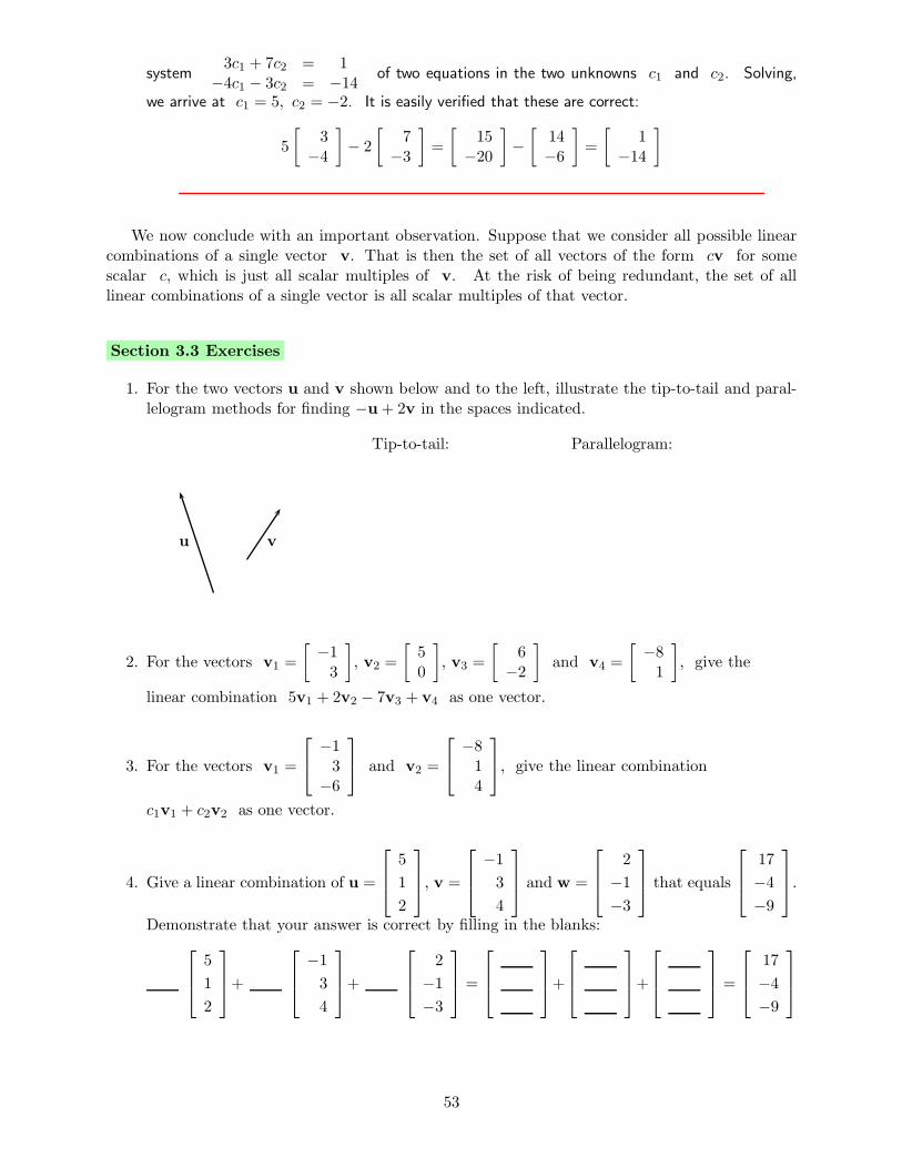
system3c1 + 7c2 = 1−4c1 − 3c2 = −14 of two equations in the two unknowns c1 and c2. Solving,
we arrive at c1 = 5, c2 = −2. It is easily verified that these are correct:
5
[
3−4
]
− 2
[
7−3
]
=
[
15−20
]
−[
14−6
]
=
[
1−14
]
We now conclude with an important observation. Suppose that we consider all possible linearcombinations of a single vector v. That is then the set of all vectors of the form cv for somescalar c, which is just all scalar multiples of v. At the risk of being redundant, the set of alllinear combinations of a single vector is all scalar multiples of that vector.
Section 3.3 Exercises
1. For the two vectors u and v shown below and to the left, illustrate the tip-to-tail and paral-lelogram methods for finding −u+ 2v in the spaces indicated.
Tip-to-tail: Parallelogram:
u v
2. For the vectors v1 =
[
−13
]
, v2 =
[
50
]
, v3 =
[
6−2
]
and v4 =
[
−81
]
, give the
linear combination 5v1 + 2v2 − 7v3 + v4 as one vector.
3. For the vectors v1 =
−13−6
and v2 =
−814
, give the linear combination
c1v1 + c2v2 as one vector.
4. Give a linear combination of u =
5
1
2
, v =
−13
4
and w =
2
−1−3
that equals
17
−4−9
.
Demonstrate that your answer is correct by filling in the blanks:
5
1
2
+
−13
4
+
2
−1−3
=
+
+
=
17
−4−9
53

5. For each of the following, find a linear combination of the vectors u1, u2 and u3 that equalsv. Conclude by giving the actual linear combination, not just some scalars.
(a) u1 =
110
, u2 =
011
, u3 =
101
, v =
123
(b) u1 =
[
3−1
]
, u2 =
[
11
]
, u3 =
[
1−1
]
, v =
[
8−6
]
6. (a) Consider the vectors u1 =
40−1
, u2 =
123
, u3 =
−265
, and w =
1158
.
If possible, find scalars a1, a2 and a3 such that a1u1 + a2u2 + a3u3 = w.
(b) Consider the vectors v1 =
40−1
, v2 =
123
, v3 =
−725
, and w =
1158
.
If possible, find scalars b1, b2 and b3 such that b1v1 + b2v2 + b3v3 = w.
(c) To do each of parts (a) and (b) you should have solved a system of equations. Let A bethe coefficient matrix for the system in (a) and let B be the coefficient matrix for thesystem in part (b). Use your calculator to find det(A) and det(B), the determinants ofmatrices A and B. You will probably find the command for the determinant in the samemenu as rref.
54

3.4 The Dot Product of Vectors, Projections
Performance Criteria:
3. (g) Find the dot product of two vectors, determine the length of a singlevector.
(h) Determine whether two vectors are orthogonal (perpendicular).
(i) Find the projection of one vector onto another, graphically or alge-braically.
The Dot Product and Orthogonality
There are two ways to “multiply” vectors, both of which you have likely seen before. One iscalled the cross product, and only applies to vectors in R
3. It is quite useful and meaningfulin certain physical situations, but it will be of no use to us here. More useful is the other method,called the dot product, which is valid in all dimensions.
Definition 3.4.1: Dot Product
Let u = [u1, u2, ..., un] and v = [v1, v2, ..., vn]. The dot product of u andv, denoted by u · v, is given by
u · v = u1v1 + u2v2 + u3v3 + · · · + unvn
The dot product is useful for a variety of things. Recall that the length of a vector v =[v1, v2, ..., vn] is given by ‖v‖ =
√
v21 + v22 + · · ·+ v2n =√v · v. Note also that v21+v22+ · · ·+v2n =
v ·v, which implies that ‖v‖ = √v · v. Perhaps the most important thing about the dot productis that the dot product of two vectors in R
2 or R3 is zero if, and only if, the two vectors are
perpendicular. In general, we make the following definition.
Definition 3.4.2: Orthogonal Vectors
Two vectors u and v in Rn are said to be orthogonal if, and only if,
u · v = 0.
⋄ Example 3.4(a): For the three vectors u =
5
−12
, v =
−13
4
and w =
2
−1−3
,
find u · v, u ·w and v ·w. Are any of the vectors orthogonal to each other?
We find thatu · v = (5)(−1) + (−1)(3) + (2)(4) = −5 + (−3) + 8 = 0,
55

u ·w = (5)(2) + (−1)(−1) + (2)(−3) = 10 + 1 + (−6) = 5,
v ·w = (−1)(2) + (3)(−1) + (4)(−3) = −2 + (−3) + (−12) = −17From the first computation we can see that u and v are orthogonal.
Projections
Given two vectors u and v, we can create a new vector w called the projection ofu onto v, denoted by projvu. This is a very useful idea, in many ways. Geometrically, we canfind projvu as follows:
• Bring u and v together tail-to-tail.
• Sketch in the line containing v, as a dashed line.
• Sketch in a dashed line segment from the tip of u to the dashed line containing v, perpen-dicular to that line.
• Draw the vector projvu from the point at the tails of u and v to the point where thedashed line segment meets v or the dashed line containing v.
Note that projvu is parallel to v; if we were to find projuv instead, the result would be parallelto u in that case. The above steps are illustrated in the following example.
⋄ Example 3.4(b): For the vectors u and v shown to the right, find the projection
projvu.u
v
We follow the above steps:
u
v
=⇒u
v
=⇒u
v
=⇒u
projvu
Projections are a bit less intuitive when the angle between the two vectors is obtuse, as seen inthe next example.
⋄ Example 3.4(c): For the vectors u and v shown to the right,find the projection projuv.
vu
We follow the steps again, noting that this time we are projecting v onto u:
56

v u
=⇒v u
=⇒v u
=⇒v u
projuv
Here we see that projuv is in the direction opposite u.
We will also want to know how to find projections algebraically:
Definition 3.4.3: The Projection of One Vector on Another
For two vectors u and v, the vector projvu is given by
projvu =u · vv · v v
Note that since both u · v and v · v are scalars, so isu · vv · v . That scalar is then multiplied
times v, resulting in a vector parallel v. if the scalar is positive the projection is in the directionof v, as shown in Example 4.2(b); when the scalar is negative the projection is in the directionopposite the vector being projected onto, as shown in Example 4.3(c).
⋄ Example 3.4(d): For the vectors u =
5
−12
and v =
2
−1−3
, find projuv.
Note that here we are projecting v onto u. first we find
v · u = (2)(5) + (−1)(−1) + (−3)(2) = 5 and u · u = 52 + (−1)2 + 22 = 30
Then
projuv =v · uu · u u =
5
30
5
−12
=
1
6
5
−12
=
56
−1613
As stated before, the idea of projection is extremely important in mathematics, and arises insituations that do not appear to have anything to do with geometry and vectors as we are thinkingof them now. You will see a clever geometric use of vectors in one of the exercises.
57

Section 3.4 Exercises
1. Consider the vectors v =
[
−27
]
and b =
[
13
]
.
(a) Draw a neat and accurate graph of v and b, with their tails at the origin, labelingeach.
(b) Use the formula to find projbv, with its components rounded to the nearest tenth.
(c) Add projbv to your graph. Does it look correct?
2. For each pair of vectors v and b below, do each of the following
i) Sketch v and b with the same initial point.
ii) Find projbv algebraically, using the formula for projections.
iii) On the same diagram, sketch the projbv you obtained in part (ii). If it does not lookthe way it should, find your error.
iv) Find projbv, and sketch it as a new sketch. Compare with your previous sketch.
(a) v =
[
31
]
, b =
[
5−2
]
(b) v =
[
−50
]
, b =
[
−21
]
(c) v =
[
31
]
, b =
[
−2−4
]
3. For each pair of vectors u and v, sketch projvu. Indicate any right angles with thestandard symbol.
u
v
(a)
uv
(b)
u
v
(c)
u
v
(d)
(u and v are orthogonal)
58

3.5 Chapter 3 Exercises
1. The purpose of this exercise is to find the distance from the point P (1,−1, 2) to the planewith equation 3x − 7y + z = 5. Of course this might seem ambiguous, since the distancedepends on where on the plane we are talking about. In order to eliminate this uncertainty, wesay that the distance from a point to a plane is DEFINED to be the smallest of the distancesbetween the point and all point on the plane. It should be intuitively clear to you that thepoint Q on the plane where this smallest distance occurs is the one where a line though thepoint and perpendicular to the plane intersects the plane. See the picture below and to theleft.
P
Q
3x− 7y + z = 5
P
Q n
R
We will solve this problem using a projection. The key idea can be seen in the picture above
and to the right. We find any point R on the plane and construct the vector−→RP . If we
then project−→RP onto the normal vector n (recall from Math 254N that the normal vector
is n = [3,−7, 1]) of the plane, the length of the projection vector will be the same as thedistance from P to Q, which is the distance from P to the plane. OK, now do it!
59

60

4 Vectors and Systems of Equations
Outcome:
4. Understand the relationship of vectors to systems of equations. Under-stand the dot product of two vectors and use it to determine whethervectors are orthogonal and to project one vector onto another.
Performance Criteria:
(a) Give the linear combination form of a system of equations.
(b) Sketch a picture illustrating the linear combination form of a systemof equations of two equations in two unknowns.
(c) Give an algebraic description of a set of a set of vectors that has beendescribed geometrically, and vice-versa.
(d) Determine whether a set of vectors is closed under vector addition; de-termine whether a set of vectors is closed under scalar multiplication.If it is, prove that it is; if it is not, give a counterexample.
(e) Give the vector equation of a line through two points in R2 or R
3 orthe vector equation of a plane through three points in R
3.
(f) Write the solution to a system of equations in vector form and deter-mine the geometric nature of the solution.
In the first two chapters of this book we began our study of linear algebra with solving systemsof linear equations; the notions and methods presented there were purely algebraic in nature. Inthe previous chapter we introduced some fundamentals of vectors. Now we will use vectors to lookat systems of equations and their solutions from a geometric perspective.
61

4.1 Linear Combination Form of a System
Performance Criterion:
4. (a) Give the linear combination form of a system of equations.
(b) Sketch a picture illustrating the linear combination form of a systemof equations of two equations in two unknowns.
It should be clear that two vectors are equal if and only if their corresponding components areequal. That is,
u1u2...un
=
v1v2...vn
if, and only if,
u1 = v1,
u2 = v2,...
un = vn
The words “if, and only if” mean that the above works “both ways” in the following sense:
• If we have two vectors of length n that are equal, then their corresponding entries are allequal, resulting in n equations.
• If we have a set of n equations, we can create a two vectors, one of whose components areall the left hand sides of the equations and the other whose components are all the right handsides of the equations, and the two vectors created this way are equal.
Using the second bullet above, we can take the system of equations below and to the left andturn them into the single vector equation shown below and to the right:
x1 + 3x2 − 2x3 = −43x1 + 7x2 + x3 = 4
−2x1 + x2 + 7x3 = 7
=⇒
x1 + 3x2 − 2x3
3x1 + 7x2 + x3
−2x1 + x2 + 7x3
=
−44
7
Considering the vector equation above and to the right, we can take the vector on the left side ofthe equation and break it into three vectors to get
x1
3x1
−2x1
+
3x2
7x2
x2
+
−2x3x3
7x3
=
−44
7
and then we can factor the scalar unknown out of each vector to get the equation
x1
1
3
−2
+ x2
3
7
1
+ x3
−21
7
=
−44
7
62

Definition 4.1.1 Linear Combination Form of a System
A system of m linear equations in n unknowns can be written as a linearcombination as follows:
a11x1 + · · · + a1nxn = b1
a21x1 + · · · + a2nxn = b2...
am1x1 + · · · + amnxn = bm
can be written as a linear combination of vectors equalling another vector:
x1
a11a21...
am1
+ x2
a12a22...
am2
+ · · ·+ xn
a1na2n...
amn
=
b1b2...bm
We will refer to this as the linear combination form of the system ofequations.
Thus the system of equations below and to the left can be rewritten in the linear combinationform shown below and to the right.
x1 + 3x2 − 2x3 = −43x1 + 7x2 + x3 = 4
−2x1 + x2 + 7x3 = 7
x1
1
3
−2
+ x2
3
7
1
+ x3
−21
7
=
−44
7
The question we originally asked for the system of linear equations was “Are there numbers x1,x2 and x3 that make all three equations true?” Now we can see this is equivalent to a differentquestion, “Is there a linear combination of the vectors [1, 3,−2], [3, 7, 1] and [−2, 1, 7] that equalsthe vector [−4, 4, 7]?”
⋄ Example 4.1(a): Give the linear combination form of the system3x1 + 5x2 = −1x1 + 4x2 = 2
of
linear equations.
The linear combination form of the system is x1
[
31
]
+ x2
[
54
]
=
[
−12
]
5
5
-5
-5
Let’s consider the system from this last example a bitmore. The goal is to solve the system of equations3x1 + 5x2 = −1x1 + 4x2 = 2
. In the past our geometric interpreta-
tion has been this: The set of solutions to the first equation isa line in R
2, and the set of solutions to the second equationis another line. The solution to the system happens to bex1 = −2, x2 = 1, and the point (−2, 1) in R
2 is the pointwhere the two lines cross. This is shown in the picture to theright.
63

Now consider the linear combination form x1
[
31
]
+ x2
[
54
]
=
[
−12
]
of the system. Let
v1 =
[
31
]
, v2 =
[
54
]
and w =
[
−12
]
. These vectors are shown in the diagram below and
to the left. The solution x1 = −2, x2 = 1 to the system is the scalars that we can use for a linearcombination of the vectors v1 and v2 to get the vector w. This is shown in the middle diagrambelow by the tip-to-tail method, and in the diagram below and to the right by the parallelogrammethod.
4
5
w
v1
v2
4
-5w = −2v1 + v2
−2v1
v2
tip-to-tail method
4
5
-5
−2v1
v2
parallelogram method
Section 4.1 Exercises
1. Give the linear combination form of each system:
(a)
x + y − 3z = 1
−3x+ 2y − z = 7
2x+ y − 4z = 0
(b)
5x1 + x3 = −12x2 + 3x3 = 0
2x1 + x2 − 4x3 = 2
2. The system of equations2x− 3y = −63x− y = 5
has solution x = 3, y = 4. Write the system
in linear combination form, then replace x and y with their values. Finally, sketch a pictureillustrating the resulting vector equation. See the explanation after Example 4.1(a) if youhave no idea what I am talking about.
64

4.2 Sets of Vectors
Performance Criterion:
4. (c) Give an algebraic description of a set of a set of vectors that has beendescribed geometrically, and vice-versa.
(d) Determine whether a set of vectors is closed under vector addition; de-termine whether a set of vectors is closed under scalar multiplication.If it is, prove that it is; if it is not, give a counterexample.
One of the most fundamental concepts of mathematics is that of sets, collections of objectscalled elements. You have probably encountered various sets of numbers, like thewhole numbers
0, 1, 2, 3, ...and the integers
Z = ...,−3,−2,−1, 0, 1, 2, 3, ....As shown above, when we describe a set by listing all or some of its elements, we enclose them with“curly brackets.” Sets are usually named by upper case letters. The above two sets are infinitesets.
Another kind of infinite set is an interval of the number line, like all real numbers between 1and 5, including 1 and 5. You have likely seen the interval notation [1, 5] for such sets. This setis also infinite, but in a different sense than the whole numbers and integers. That difference is notof concern to us here, but some of you may encounter that idea again. Of course, there are alsofinite sets like 2, 4, 6, 8.
There will be a time soon when we will be very interested in sets of vectors, both finite andinfinite. For example we might be interested in the finite set
A =
100
,
110
,
or the infinite set of all vectors of the form
[
a
2a
]
, where a is any real number. Let’s examine
this set a bit more.
⋄ Example 4.2(a): Let B be the set of all vectors of the form
[
a
2a
]
, where a is any
real number. Are the vectors u =
[
310
]
and v =
[
−2−4
]
in B?
Because 2(3) 6= 10, u is not in B. But 2(−2) = −4, so v is in B.
⋄ Example 4.2(b): Let C be the set of all vectors of the form
[
a
a+ 1
]
, where a is any
real number. Are the vectors u =
[
34
]
and v =
[
−2−1
]
in C?
3 + 1 = 4 and −2 + 1 = −1, so both u and v are in C.
65

In the future we will also be very interested in this question: Given an infinite set of vectors, isthe sum of any two vectors a vector that is also in the set? When faced with such a question weshould do one of two things:
• Give two specific vectors that are in the set, and show that their sum is not.
• Give two arbitray (general) vectors in the set and show that their sum is also in the set.
The following Examples illustrate these.
⋄ Example 4.2(c): Let B be the set of all vectors of the form
[
a
2a
]
, where a is any
real number. Determine whether the sum of any two vectors in B is also in B.
The vectors
[
36
]
and
[
−2−4
]
are both in B, and their sum
[
12
]
is as well. We may
have just gotten lucky, though, and maybe the sum of any two vectors in B is not necessarilyin B. Let’s see if the sum of two arbitrary vectors in B is in B:
[
a
2a
]
+
[
b
2b
]
=
[
a+ b
2a+ 2b
]
=
[
a+ b
2(a+ b)
]
=
[
c
2c
]
,
where c = a+ b. Therefore the sum of any two vectors in B is a vector in B.
⋄ Example 4.2(d): Let C be the set of all vectors of the form
[
a
a+ 1
]
, where a is any
real number. Is the sum of any two vectors in C also a vector in C?
The vectors
[
34
]
and
[
−2−1
]
are both in C, as shown in Example 4.2(b). Their sum is
the vector
[
13
]
, which is not in C because 1 + 1 6= 3. Thus the sum of any two vectors in
C is not necessarily another vector in C.
⋄ Example 4.2(e): Let D be the set of all vectors of the form
[
x
y
]
, where x ≥ 0 and
y ≥ 0. Is the sum of any two vectors in D also a vector in D?
Suppose that
[
x1y1
]
and
[
x2y2
]
are both in D, so all of x1, y1, x2, y2 are greater than or
equal to zero. Clearly x1 + x2 ≥ 0 and y1 + y2 ≥ 0, so their sum
[
x1 + x2y1 + y2
]
is in D.
Given a set of vectors, we are also interested in whether a scalar multiple of a vector in the setis also in the set. In the next example we determine whether that is the case for the set D fromthe previous example.
66

4.3 Vector Equations of Lines and Planes
Performance Criterion:
4. (e) Give the vector equation of a line through two points in R2 or R
3 orthe vector equation of a plane through three points in R
3.
The idea of a linear combination does more for us than just give another way to interpret asystem of equations. The set of points in R
2 satisfying an equation of the form y = mx + b isa line; any such equation can be rearranged into the form ax+ by = c. (The values of b in thetwo equations are clearly not the same.) But if we add one more term to get ax + by + cz = d,with the (x, y, z) representing the coordinates of a point in R
3, we get the equation of a plane,not a line! In fact, we cannot represent a line in R
3 with a single scalar equation. The objectof this section is to show how we can represent lines, planes and higher dimensional objects calledhyperplanes using linear combinations of vectors.
For the bulk of this course, we will think of most vectors as position vectors. (Remember, thismeans their tails are at the origin.) We will also think of each position vector as correspondingto the point at its tip, so the coordinates of the point will be the same as the components of the
vector. Thus, for example, in R2 the vector x =
[
x1x2
]
=
[
1−3
]
corresponds to the ordered
pair (x1, x2) = (1,−3).
⋄ Example 4.3(a): Graph the set of points corresponding to all vectors x of the form
x = t
[
1−3
]
, where t represents any real number.
We already know that when t = 1 the the vector x correspondsto the point (1,−3). We then let t = −2,−1, 0, 2 anddetermine the corresponding vectors x:
t = −2 ⇒ x =
[
−26
]
, t = −1 ⇒ x =
[
−13
]
t = 0 ⇒ x =
[
00
]
t = 2 ⇒ x =
[
2−6
]
5
5
-5
-5
t = −2
t = −1t = 0
t = 1
t = 2
x
y
These vectors correspond to the points with ordered pairs (−2, 6), (−1, 3), (0, 0) and (2,−6).When we plot those points and the point (1,−3) that we already had, we get the line shownabove and to the right.
It should be clear from the above example that we could create a line through the origin in any
direction by simply replacing the vector
[
1−3
]
with a vector in the direction of the desired line.
The next question is, “how do we get a line that is not through the origin?” The next exampleillustrates how this is done.
69

⋄ Example 4.3(b): Graph the set of points corresponding to all vectors x of the form
x =
[
23
]
+ t
[
−31
]
, where t represents any real number.
Performing the scalar multiplication by t and adding the twovectors, we get
x =
[
2− 3t3 + t
]
.
These vectors then correspond to all points of the form (2 −3t, 3 + t). When t = 0 this is the point (2, 3) so our lineclearly passes through that point. Plotting the points obtainedwhen we let t = −1, 1, 2 and 3, we see that we will get theline shown to the right.
5
5
-5
-5
t = −1
t = 0
t = 1
t = 2
t = 3
P
Q x
y
Now let’s make two observations about the set of points represented by the set of all vectors
x =
[
23
]
+ t
[
−31
]
, where t again represents any real number. These vectors correspond to
the ordered pairs of the form (4− 3t,−2 + t). Plotting these results in the line through the point
(2, 3) and in the direction of the vector
[
−31
]
. This is not a coincidence. Consider the line
shown below and to the left, containing the points P and Q. If we let u =−−→OP and v =
−−→PQ,
then the points P and Q correspond to the vectors u and u+ v (in standard position, whichyou should assume we mean from here on), as shown in the second picture. From this you shouldbe able to see that if we consider all the vectors x defined by x = u+ tv as t ranges over allreal numbers, the resulting set of points is our line! This is shown in the third picture, where t isgiven the values −1, 1
2 and 2.
O
P
Q
O
P
Q
u =−−→OP
v =−−→PQ
u+ v
O
PQ
u
v
−v
u
u+ (−1)v
u+ 2v
u+ 1
2v
Now this may seem like an overly complicated way to describea line, but with a little thought you should see that the ideatranslates directly to three (and more!) dimensions, as shownin the picture to the right. This is all summarized below: O
P
Q
uv
70

Lines in R2 and R
3
The vector equation of a line through two points P and Q in R2 and
R3 (and even higher dimensions) is
x =−−→OP + t
−−→PQ.
By this we mean that the line consists of all the points corresponding to the
position vectors x as t varies over all real numbers. The vector−−→PQ is called
the direction vector of the line.
⋄ Example 4.3(c): Give the vector equation of the line in R2 through the points P (−4, 1) and
Q(5, 3).
We need two vectors, one from the origin out to the line, and one in the direction of the line. For
the first we will use−−→OP , and for the second we will use
−−→PQ = [9, 2]. We then have
x =−−→OP + t
−−→PQ =
[
−41
]
+ t
[
92
]
,
where x = [x1, x2] is the position vector corresponding to any point (x1, x2) on the line.
⋄ Example 4.3(d): Give a vector equation of the line in R3 through the points (−5, 1, 2) and
(4, 6,−3).
Letting P be the point (−5, 1, 2) and Q be the point (4, 6,−3), we get−−→PQ = 〈9, 5,−5〉.
The vector equation of the line is then
x =−−→OP + t
−−→PQ =
−512
+ t
95−5
,
where x = [x1, x2, x3] is the position vector corresponding to any point (x1, x2, x3) on theline. The first vector can be any point on the line, so it could be the vector [4, 6,−3] insteadof [−5, 1, 2], and the second vector is a direction vector, so can be any scalar multiple ofd = [9, 5,−5].
The same general idea can be used to describe a plane in R3. Before seeing how that works,
let’s define something and look at a situation in R2. We say that two vectors are parallel if one
is a scalar multiple of the other. Now suppose that v and w are two vectors in R2 that are not
parallel (and neither is the zero vector either), as shown in the picture to the left below, and letP be the randomly chosen point in R
2 shown in the same picture. The next picture shows that alinear combination of v and w can be formed that gives us a vector sv+ tw corresponding tothe point P . In this case the scalar s is positive and less than one, and t is positive and greaterthan one. The third and fourth pictures show the same thing for another point Q, with boths being negative and t positive in that case. It should now be clear that any point in R
2 canbe obtained in this manner.
71
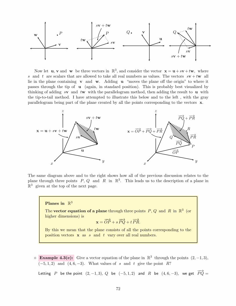
v
w P
svtw
sv + tw
P
u
vQ
sv
tw
sv + tw
Q
Now let u, v and w be three vectors in R3, and consider the vector x = u+ sv+ tw, where
s and t are scalars that are allowed to take all real numbers as values. The vectors sv+ tw alllie in the plane containing v and w. Adding u “moves the plane off the origin” to where itpasses through the tip of u (again, in standard position). This is probably best visualized bythinking of adding sv and tw with the parallelogram method, then adding the result to u withthe tip-to-tail method. I have attempted to illustrate this below and to the left , with the grayparallelogram being part of the plane created by all the points corresponding to the vectors x.
u
sv
tw
sv + tw
x = u+ sv+ tw
xy
z
P
Q
R
−−→OP
−−→PQ
−→PR
−−→PQ+
−→PR
x =−−→OP +
−−→PQ+
−→PR
xy
z
The same diagram above and to the right shows how all of the previous discussion relates to theplane through three points P , Q and R in R
3. This leads us to the description of a plane inR3 given at the top of the next page.
Planes in R3
The vector equation of a plane through three points P , Q and R in R3 (or
higher dimensions) is
x =−−→OP + s
−−→PQ+ t
−→PR.
By this we mean that the plane consists of all the points corresponding to theposition vectors x as s and t vary over all real numbers.
⋄ Example 4.3(e): Give a vector equation of the plane in R3 through the points (2,−1, 3),
(−5, 1, 2) and (4, 6,−3). What values of s and t give the point R?
Letting P be the point (2,−1, 3), Q be (−5, 1, 2) and R be (4, 6,−3), we get−−→PQ =
72

[−7, 2,−1] and−→PR = [2, 7,−6]. The vector equation of the plane is then
x =−−→OP + s
−−→PQ+ t
−→PR =
2−13
+ s
−72−1
+ t
27−6
,
where x = [x1, x2, x3] is the position vector corresponding to any point (x1, x2, x3) on theplane. It should be clear that there are other possibilities for this. The first vector in the equationcould be any of the three position vectors for P , Q or R. The other two vectors could be anytwo vectors from one of the points to another.
The vector corresponding to point R is−−→OR, which is equal to x =
−−→OP +
−→PR (think about
that), so s = 0 and t = 1.
We now summarize all of the ideas from this section.
Lines in R2 and R
3, Planes in R3
Let u and v be vectors in R2 or R
3 with v 6= 0. Then the set of pointscorresponding to the vector x = u + tv as t ranges over all real numbers isa line through the point corresponding to u and in the direction of v. (So ifu = 0 the line passes through the origin.)
Let u, v and w be vectors R3, with v and w being nonzero and not
parallel. (That is, not scalar multiples of each other.) Then the set of pointscorresponding to the vector x = u+ sv + tw as s and t range over all realnumbers is a plane through the point corresponding to u and containing thevectors v and w. (If u = 0 the plane passes through the origin.)
Section 4.3 Exercises
1. For each of the following, give the vector equation of the line or plane described.
(a) The line through the two points P (3,−1, 4) and Q(2, 6, 0) in R3.
(b) The plane through the points P (3,−1, 4), Q(2, 6, 0) and R(−1, 0, 3) in R3.
(c) The line through the points P (3,−1) and Q(6, 0) in R2.
2. Find another point in the plane containing P1(−2, 1, 5), P2(3, 2, 1) and P3(4,−2,−3). Showclearly how you do it. (Hint: Find and use the vector equation of the plane.)
3. “Usually” a vector equation of the form x = p+ su+ tv gives the equation of a plane in R3.
(a) Under what conditions on p and/or u and/or v would this be the equation of a line?
(b) Under what conditions on p and/or u and/or v would this be the equation of a planethrough the origin?
73

4.4 Interpreting Solutions to Systems of Linear Equations
Performance Criterion:
4. (f) Write the solution to a system of equations in vector form and deter-mine the geometric nature of the solution.
We begin this section by considering the following two systems of equations.
3x1 − 3x2 + 3x3 = 9
2x1 − x2 + 4x3 = 7
3x1 − 5x2 − x3 = −3
x1 − x2 + 2x3 = 1
−3x1 + 3x2 − 6x3 = −32x1 − 2x2 + 4x3 = 2
The augmented matrices for these two systems reduce to the following matrices, respectively.
1 0 3 40 1 2 10 0 0 0
1 −1 2 10 0 0 00 0 0 0
Let’s look at the first system. x3 is a free variable, and x1 and x2 are leading variables. Thegeneral solution is x1 = −3t + 4, x2 = −2t + 1, x3 = t. Algebraically, x1, x2 and x3 are justnumbers, but we can think of (x1, x2, x3) as a point in R
3. The corresponding position vector is
x =
x1
x2
x3
=
4− 3t
1− 2t
t
=
4
1
0
+
−3t−2t
t
=
4
1
0
+ t
−3−21
We will call this the vector form of the solution to the system of equations. The beauty ofexpressing the solutions to a system of equations in vector form is that we can see what the set ofall solutions looks like. In this case, the set of solutions is the set of all points in R
3 on the linethrough (4, 1, 0) and with direction vector [−3,−2, 1].
⋄ Example 4.4(a): The general solution to the second system of equations is x1 = 1+s−2t,x2 = s, x3 = t. Express the solution on vector form and determine the geometric nature ofthe solution set in R
3.
A process like the one just carried out leads to the general solution with position vector
x =
x1
x2
x2
=
1
0
0
+ s
1
1
0
+ t
−20
1
(Check to make sure that you understand how this was arrived at.) Here the set of solutions isthe set of all points in R
3 on the plane through (1, 0, 0) with direction vectors [1, 1, 0] and[−2, 0, 1].
74

Now recall that the three equations from this last example,
x1 − x2 + 2x3 = 1
−3x1 + 3x2 − 6x3 = −32x1 − 2x2 + 4x3 = 2
represent three planes in R3, and when we solve the system we are looking for all points in R
3 thatare solutions to all three equations. Our results tell us that the set of solution points in this caseis itself a plane, which can only happen if all three equations represent the same plane. If you lookat them carefully you can see that the second and third equations are multiples of the first, so thepoints satisfying them also satisfy the first equation.
⋄ Example 4.4(b): The general solution to the second system of equations is x1 = 1+s−2t,x2 = s, x3 = t. Express the solution in vector form and determine the geometric nature ofthe solution set in R
3.
A process like the one just carried out leads to the general solution with position vector
x =
x1
x2
x3
=
1
0
0
+ s
1
1
0
+ t
−20
1
(Check to make sure that you understand how this was arrived at.) Here the set of solutions isthe set of all points in R
3 on the plane through (1, 0, 0) with direction vectors [1, 1, 0] and[−2, 0, 1].
⋄ Example 4.4(c): Give the vector form of the solution to the system
3x2 − 6x3 − 4x4 − 3x5 = −5x1 − 3x2 + 10x3 + 4x4 + 4x5 = 2
2x1 − 6x2 + 20x3 + 2x4 + 8x5 = −8
The augmented matrix of the system reduces to
1 0 4 0 1 −30 1 −2 0 −1 1
0 0 0 1 0 2
We can see that x3 and x5 are free variables, and we can also see that x4 = 2. Lettingx5 = t and x3 = s, x2 = 1 + 2s+ t and x1 = −3− 4s− t. Therefore
x =
x1
x2
x3
x4
x5
=
−31
0
2
0
+ s
−42
1
0
0
+ t
−11
0
0
1
75

How do we interpret this result geometrically? The set of points (x1, x2, x3, x4, x5) representsa two-dimensional plane in five-dimensional space. We could also have ended up with one, three orfour dimensional “plane”, often called a hyperplane, in five-dimensional space.
Section 4.4 Exercises
1. For each of the following, a student correctly finds the given the general solution (x1, x2, x3) toa system of three equations in three unknowns. Give the vector form of the solution, thentell whether the set of all particular solutions is a point, line or plane.
(a) x1 = s− t+ 5, x2 = s, x3 = t (b) x1 = 2t+ 5, x2 = t, x3 = −1
(c) x1 = s− 2t+ 5, x2 = s, x3 = t
76

4.5 Chapter 4 Exercises
1. Consider the plane in R3 with vector equation x =
5
−12
+ s
1
7
−4
+ t
−2−53
.
The point (18.9, 50.4,−28.1) lies on this plane - find the values of s and t that give thispoint. You may wish to use the following hints.
• Where do the values 18.9, 50.4 and −28.1 go?
• How many unknowns are you solving for? Based on this, how many columns shouldyour augmented matrix have?
77

78

5 Matrices and Vectors
Outcome:
5. Understand matrices, their algebra, and their action on vectors. Use ma-trices to solve problems.
Performance Criteria:
(a) Give the dimensions of a matrix. Identify a given entry, row or columnof a matrix.
(b) Identify matrices as square, upper triangular, lower triangular, sym-metric, diagonal. Give the transpose of a given matrix; know thenotation for the transpose of a matrix.
(c) Know when two matrices can be added or subtracted; add or subtracttwo matrices when possible.
(d) Multiply a matrix times a vector.
(e) Give the identity matrix (for a given dimensional space) and its effectwhen a vector is multiplied by it.
(f) Determine whether a matrix is a projection matrix, rotation matrix,or neither, by its action on a few vectors.
(g) Plot a discrete function. Give derivative and integral matrices, filtermatrices.
79
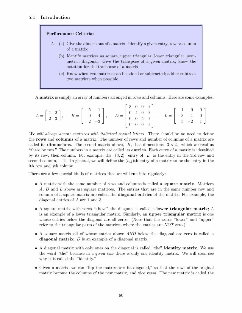
5.1 Introduction
Performance Criteria:
5. (a) Give the dimensions of a matrix. Identify a given entry, row or columnof a matrix.
(b) Identify matrices as square, upper triangular, lower triangular, sym-metric, diagonal. Give the transpose of a given matrix; know thenotation for the transpose of a matrix.
(c) Know when two matrices can be added or subtracted; add or subtracttwo matrices when possible.
Amatrix is simply an array of numbers arranged in rows and columns. Here are some examples:
A =
[
1 2
2 3
]
, B =
−5 1
0 4
2 −3
, D =
3 0 0 0
0 4 0 0
0 0 5 0
0 0 0 6
, L =
1 0 0
−3 1 0
5 −2 1
We will always denote matrices with italicized capital letters. There should be no need to definethe rows and columns of a matrix. The number of rows and number of columns of a matrix arecalled its dimensions. The second matrix above, B, has dimensions 3 × 2, which we read as“three by two.” The numbers in a matrix are called its entries. Each entry of a matrix is identifiedby its row, then column. For example, the (3, 2) entry of L is the entry in the 3rd row andsecond column, −2. In general, we will define the (i, j)th entry of a matrix to be the entry in theith row and jth column.
There are a few special kinds of matrices that we will run into regularly:
• A matrix with the same number of rows and columns is called a square matrix. MatricesA, D and L above are square matrices. The entries that are in the same number row andcolumn of a square matrix are called the diagonal entries of the matrix. For example, thediagonal entries of A are 1 and 3.
• A square matrix with zeros “above” the diagonal is called a lower triangular matrix; Lis an example of a lower triangular matrix. Similarly, an upper triangular matrix is onewhose entries below the diagonal are all zeros. (Note that the words “lower” and “upper”refer to the triangular parts of the matrices where the entries are NOT zero.)
• A square matrix all of whose entries above AND below the diagonal are zero is called adiagonal matrix. D is an example of a diagonal matrix.
• A diagonal matrix with only ones on the diagonal is called “the” identity matrix. We usethe word “the” because in a given size there is only one identity matrix. We will soon seewhy it is called the “identity.”
• Given a matrix, we can “flip the matrix over its diagonal,” so that the rows of the originalmatrix become the columns of the new matrix, and vice versa. The new matrix is called the
80
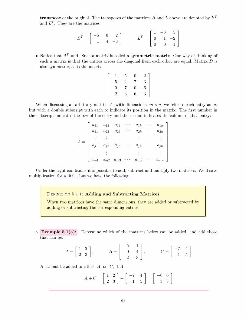
transpose of the original. The transposes of the matrices B and L above are denoted by BT
and LT . They are the matrices
BT =
[ −5 0 2
1 4 −3
]
LT =
1 −3 5
0 1 −20 0 1
• Notice that AT = A. Such a matrix is called a symmetric matrix. One way of thinking ofsuch a matrix is that the entries across the diagonal from each other are equal. Matrix D isalso symmetric, as is the matrix
1 5 0 −25 −4 7 3
0 7 0 −6−2 3 −6 −3
When discussing an arbitrary matrix A with dimensions m× n we refer to each entry as a,but with a double subscript with each to indicate its position in the matrix. The first number inthe subscript indicates the row of the entry and the second indicates the column of that entry:
A =
a11 a12 a13 · · · a1k · · · a1n
a21 a22 a23 · · · a2k · · · a2n...
......
...
aj1 aj2 aj3 · · · ajk · · · ajn...
......
...
am1 am2 am3 · · · amk · · · amn
Under the right conditions it is possible to add, subtract and multiply two matrices. We’ll savemultiplication for a little, but we have the following:
Definition 5.1.1: Adding and Subtracting Matrices
When two matrices have the same dimensions, they are added or subtracted byadding or subtracting the corresponding entries.
⋄ Example 5.1(a): Determine which of the matrices below can be added, and add thosethat can be.
A =
[
1 2
2 3
]
, B =
−5 1
0 4
2 −3
, C =
[ −7 4
1 5
]
B cannot be added to either A or C, but
A+ C =
[
1 2
2 3
]
+
[ −7 4
1 5
]
=
[ −6 6
3 8
]
81

It should be clear that A and C could be subtracted, and that A+C = C+A but A−C 6= C−A.
Section 5.1 Exercises
1. (a) Give the dimensions of matrices A, B and C in Exercise 3 below.
(b) Give the entries b13 and c32 of the matrices B and C in Exercise 3 below.
2. Give examples of each of the following types of matrices.
(a) lower triangular (b) diagonal
(c) symmetric (d) identity
(e) upper triangular but not diagonal (f) symmetric but without any zero entries
(g) symmetric but not diagonal (h) diagonal but not a multiple of an identity
3. Give the transpose of each matrix. Use the correct notation to denote the transpose.
A =
1 0 5−3 1 −24 7 0
B =
1 0−3 14 7
C =
1 0 −1 3−3 1 2 04 7 0 −2
D =
1 −31 21 4
4. Give all possible sums and differences of matrices from Exercise 3.
82

5.2 Multiplying a Matrix Times a Vector
Performance Criteria:
5. (d) Multiply a matrix times a vector.
(e) Give the identity matrix (for a given dimensional space) and its effectwhen a vector is multiplied by it.
In Section 6.1 we will find out how to multiply a matrix times another matrix but, for nowwe’ll multiply only matrices times vectors. This is not to say that doing so is a minor step on theway to learning to multiply matrices; multiplying a matrix times a vector is in some sense THEfoundational operation of linear algebra.
Before getting into how to do this, we need to devise a useful notation. Consider the matrix
A =
a11 · · · a1n
a21 · · · a2n...
. . ....
am1 · · · amn
Each column of A, taken by itself, is a vector. We’ll refer to the first column as the vector a∗1,with the asterisk * indicating that the row index will range through all values, and the 1 indicatingthat the values all come out of column one. Of course a∗2 denotes the second column, and so on.Similarly, a1∗ will denote the first row, a1∗ the second row, etc. Technically speaking, the rowsare not vectors, but we’ll call them row vectors and we’ll call the columns column vectors. Ifwe use just the word vector, we will mean a column vector.
⋄ Example 5.2(a): Give a2∗ and a∗3 for the matrix A =
−5 3 4 −17 5 2 4
2 −1 −6 0
a2∗ =[
7 5 2 4]
and a∗3 =
4
2
−6
Definition 5.2.1: Matrix Times a Vector
An m×n matrix A can be multiplied times a vector x with n components.The result is a vector with m components, the ith component being the dotproduct of the ith row of A with x, as shown below.
a11 · · · a1n
a21 · · · a2n...
. . ....
am1 · · · amn
x1
x2...
xn
=
a11x1 + · · ·+ a1nxn
a21x1 + · · ·+ a2nxn...
am1x1 + · · ·+ amnxn
=
a1∗ · xa2∗ · x
...
am∗ · x
83

⋄ Example 5.2(b): Multiply
3 0 −1−5 2 4
1 −6 0
2
1
−7
.
3 0 −1−5 2 4
1 −6 0
2
1
−7
=
(3)(2) + (0)(1) + (−1)(−7)(−5)(2) + (2)(1) + (4)(−7)(1)(2) + (−6)(1) + (0)(−7)
=
13
−36−4
There is no need for the matrix multiplying a vector to be square, but when it is not, the resultingvector is not the same length as the original vector:
⋄ Example 5.2(c): Multiply
[
7 −4 2
−1 0 6
]
3
−51
.
[
7 −4 2
−1 0 6
]
3
−51
=
[
(7)(3) + (−4)(−5) + (2)(1)
(−1)(3) + (0)(−5) + (6)(1)
]
=
[
43
3
]
Multiplication of vectors by matrices has the following important properties, which are easilyverified.
Theorem 5.2.2
Let A and B be matrices, x and y be vectors, and c be any scalar.Assuming that all the indicated operations below are defined (possible), then
(a) A(x+ y) = Ax+Ay (b) A(cx) = c(Ax)
(b) (A+B)x = Ax+Bx
We now come to a very important idea that depends on the first two properties above. Whenwe act on a mathematical object with another object, the object doing the “acting on” is oftencalled an operator. Some operators you are familiar with are the derivative operator and theantiderivative operator (indefinite integral), which act on functions to create other functions. Notethat the derivative operator has the following two properties, for any functions f and g and realnumber c:
d
dx(f + g) =
df
dx+
dg
dx,
d
dx(cf) = c
df
dx
These are the same as the first two properties for multiplication of a vector by a matrix. A matrixcan be thought of as an operator that operates on vectors by multiplying them. The first twoproperties of multiplication of a vector by a matrix, as well as the corresponding properties of
84

the derivative, are called the linearity properties. Both the derivative operator and matrixmultiplication operator are then called linear operators. This is why this subject is called linearalgebra!
There is another way to compute a matrix times a vector. It is not as efficient to do by handas what we have been doing so far, but it will be very important conceptually quite soon. Usingour earlier definition of a matrix A times a vector x, we see that
Ax =
a11x1 + · · ·+ a1nxn
a21x1 + · · ·+ a2nxn...
am1x1 + · · ·+ amnxn
=
a11x1
a21x1...
am1x1
+
a21x2
a22x2...
am2x2
+ · · ·+
a1nxn
a2nxn...
amnxn
= x1
a11
a21...
am1
+ x2
a21
a22...
am2
+ · · · + xn
a1n
a2n...
amn
= x1a∗1 + x2a∗2 + · · ·+ xna∗n
Let’s think about what the above shows. It gives us the result below, which is illustrated inExamples 5.2(d) and (e).
Linear Combination Form of a Matrix Times a Vector
The product of a matrix A and a vector x is a linear combination of thecolumns of A, with the scalars being the corresponding components of x.
⋄ Example 5.2(d): Give the linear combination form of
[
7 −4 2
−1 0 6
]
3
−51
.
[
7 −4 2
−1 0 6
]
3
−51
= 3
[
7
−1
]
− 5
[
−40
]
+ 1
[
2
6
]
⋄ Example 5.2(e): Give the linear combination form of
1 3 −23 7 1−2 1 7
x1x2x3
.
1 3 −23 7 1−2 1 7
x1x2x3
= x1
13−2
+ x2
371
+ x3
−217
85

Section 5.2 Exercises
1. Multiply
1 0 −1−3 1 24 7 −2
5−12
and
[
3 −4 0−1 5 1
]
−152
2. Find a matrix A such that A
[
x1x2
]
=
[
3x1 − 5x2x1 + x2
]
.
3. Give the 3× 3 identity matrix I. For any vector x, Ix = .
86

5.3 Actions of Matrices on Vectors: Transformations in R2
In the previous section we defined a matrix times a vector in a purely computational sense. To putthat operation to use we want to think of a matrix as acting on a vector to create a new vector.One might also think of this as a matrix transforming a vector into another vector.
In general, when a matrix acts on a vector the resulting vector will have a different directionand length than the original vector. There are a few notable exceptions to this:
• The matrix that acts on a vector without actually changing it at all is called the identitymatrix. Clearly, then, when the identity matrix acts on a vector, neither the direction ormagnitude is changed.
• A matrix that rotates every vector in R2 through a fixed angle θ is called a rotation
matrix. In this case the direction changes, but not the magnitude. (Of course the directiondoesn’t change if θ = 0 and, in some sense, if θ = 180. In the second case, even thoughthe direction is opposite, the resulting vector is still just a scalar multiple of the original.)
• For most matrices there are certain vectors, called eigenvectors whose directions don’tchange (other than perhaps reversing) when acted on by by the matrix under consideration.In those cases, the effect of multiplying such a vector by the matrix is the same as multiplyingthe vector by a scalar. This has very useful applications.
87

5.4 Chapter 5 Exercises
1. Let A =
[
3 −1−4 0
]
, u =
[
1
1
]
, v =
[
−12
]
, w =
[
0
2
]
.
(a) Find Au, Av and Aw.
(b) Plot and label u, v, w, Au, Av and Aw on ONE R2 coordinate grid.
You should not see any special relationship between the vectors x and Ax (where x is torepresent any vector) here.
2. Let B =
[√32 −1
2
12
√32
]
, u =
[
4
0
]
, v =
[
−31
]
, w =
[
3
4.5
]
.
(a) Find Bu, Bv and Bw, with their components as decimals to the nearest tenth.
(b) Plot and label u, v, w, Bu, Bv and Bw on one R2 coordinate grid.
(c) You should be able to see that B does not seem to change the length of a vector. Toverify this, find ‖w‖ and ‖Bw‖ to the nearest hundredth.
(d) What does the matrix B seem to do to every vector?
(e) The entries of B should look familiar to you. What is special about 12 and
√32 ?
3. Let C =
[
1625
1225
1225
925
]
, u =
[
4
0
]
, v =
[
−31
]
, w =
[
4.5
6
]
.
(a) Find Cu, Cv and Cw, with their components as decimals to the nearest tenth.
(b) Plot and label u, v, w, Cu, Cv and Cw on one R2 coordinate grid.
(c) What does the matrix C seem to do to every vector? (Does the magnitude change?Does the direction change?)
(d) Can you see the role of the entries of the matrix here?
4. Again let A =
[
3 −1−4 0
]
, (see Exercise 8) but let u =
[
−11
]
, v =
[
1
2
]
, w =
[
1
4
]
.
(a) Find Au, Av and Aw.
(b) Plot and label u, v, w, Au, Av and Aw on one R2 coordinate grid.
(c) For one of the vectors, there should be no apparent relationship between the vector andthe result when it is multiplied by the matrix. Discuss what happened to the directionand magnitude of each of the other two vectors when the matrix acted on it.
(d) Pick one of your two vectors for which something special happened and multiply it bythree, and multiply the result by A; what is the effect of multiplying by A in thiscase?
(e) Pick the other special vector, multiply it by five, then by A. What effect does multi-plying by A have on the vector?
94

6 Matrix Multiplication
Outcome:
6. Understand the algebra of matrices, understand and compute the inverseof a matrix, use matrices to solve problems.
Performance Criteria:
(a) Know when two matrices can be multiplied, and know that matrixmultiplication is not necessarily commutative.
(b) Multiply two matrices “by hand.”
(c) Multiply two matrices “by hand” using all three of the linear com-bination of columns, outer product, and linear combination of rowsmethods.
(d) Determine whether two matrices are inverses without finding the in-verse of either.
(e) Find the inverse of a 2×2 matrix using the formula.
(f) Find the inverse of a matrix using the Gauss-Jordan method. De-scribe the Gauss-Jordan method for finding the inverse of a matrix.
(g) Give the geometric or algebraic representations of the inverse orsquare of a rotation in R
2. Demonstrate that the geometric andalgebraic versions are the same.
(h) Give the incidence matrix of a graph or digraph. Given the incidencematrix of a graph or digraph, identify the vertices and edges usingcorrect notation, and draw the graph.
(i) Determine the number of k-paths from one vertex of a graph to an-other. Solve problems using incidence matrices.
95
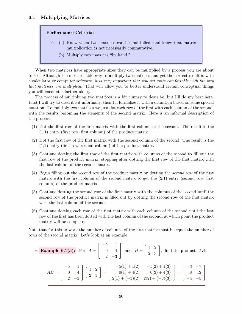
6.1 Multiplying Matrices
Performance Criteria:
6. (a) Know when two matrices can be multiplied, and know that matrixmultiplication is not necessarily commutative.
(b) Multiply two matrices “by hand.”
When two matrices have appropriate sizes they can be multiplied by a process you are aboutto see. Although the most reliable way to multiply two matrices and get the correct result is witha calculator or computer software, it is very important that you get quite comfortable with the waythat matrices are multiplied. That will allow you to better understand certain conceptual thingsyou will encounter farther along.
The process of multiplying two matrices is a bit clumsy to describe, but I’ll do my best here.First I will try to describe it informally, then I’ll formalize it with a definition based on some specialnotation. To multiply two matrices we just dot each row of the first with each column of the second,with the results becoming the elements of the second matrix. Here is an informal description ofthe process:
(1) Dot the first row of the first matrix with the first column of the second. The result is the(1,1) entry (first row, first column) of the product matrix.
(2) Dot the first row of the first matrix with the second column of the second. The result is the(1,2) entry (first row, second column) of the product matrix.
(3) Continue dotting the first row of the first matrix with columns of the second to fill out thefirst row of the product matrix, stopping after dotting the first row of the first matrix withthe last column of the second matrix.
(4) Begin filling out the second row of the product matrix by dotting the second row of the firstmatrix with the first column of the second matrix to get the (2,1) entry (second row, firstcolumn) of the product matrix.
(5) Continue dotting the second row of the first matrix with the columns of the second until thesecond row of the product matrix is filled out by dotting the second row of the first matrixwith the last column of the second.
(6) Continue dotting each row of the first matrix with each column of the second until the lastrow of the first has been dotted with the last column of the second, at which point the productmatrix will be complete.
Note that for this to work the number of columns of the first matrix must be equal the number ofrows of the second matrix. Let’s look at an example.
⋄ Example 6.1(a): For A =
−5 1
0 4
2 −3
and B =
[
1 2
2 3
]
, find the product AB.
AB =
−5 1
0 4
2 −3
[
1 2
2 3
]
=
−5(1) + 1(2) −5(2) + 1(3)
0(1) + 4(2) 0(2) + 4(3)
2(1) + (−3)(2) 2(2) + (−3)(3)
=
−3 −78 12
−4 −5
96

In order to make a formal definition of matrix multiplication, we need to develop a bit of specialnotation. Given a matrix
A =
a11 a12 · · · a1n
a21 a22 · · · a2n...
......
am1 am2 · · · amn
,
we refer to, for example the third row as A3∗. Here the first subscript 3 indicates that we areconsidering the third row, and the ∗ indicates that we are taking the elements from the third rowin all columns. Therefore A3∗ refers to a 1× n matrix. Similarly, a∗2 is the vector that is thesecond column of A. So we have
A3∗ =[
a31 a32 · · · a3n]
a∗2 =
a12a22...
a2m
A 1×n matrix like A3∗ can be thought of like a vector; in fact, we sometimes call such a matrixa row vector. Note that the transpose of such a vector is a column vector. We then define aproduct like product Ai∗b∗j by
Ai∗b∗j = ATi∗ · b∗j = ai1b1j + ai2b2j + ai3b3j + · · ·+ ainbnj =
n∑
k=1
aikbkj
This is the basis for the following formal definition of the product of two matrices.
Definition 6.1.1: Matrix Multiplication
Let A be an m×n matrix whose rows are the vectors A1∗, A2∗, ..., Am∗ andlet B be an n × p matrix whose columns are the vectors b∗1,b∗2, ...,b∗p.Then AB is the m× p matrix
AB =
a11 a12 · · · a1n
a21 a22 · · · a2n...
.... . .
...
am1 am2 · · · amn
b11 b12 · · · b1p
b21 b22 · · · b2p...
.... . .
...
bn1 bn2 · · · bnp
=
A1∗
A2∗...
Am∗
[ b∗1 b∗2 b∗3 · · · b∗p ]
=
A1∗b∗1 A1∗b∗2 · · · A1∗b∗p
A2∗b∗1 A2∗b∗2 · · · A2∗b∗p...
.... . .
...
Am∗b∗1 Am∗b∗2 · · · Am∗b∗p
For the above computation to be possible, products in the last matrix.Thisimplies that the number of columns of A must equal the number of rows of B.
97
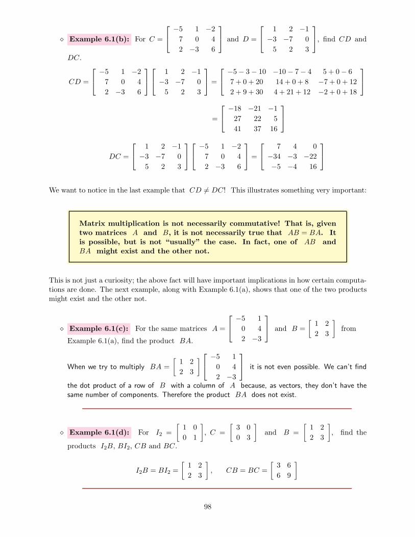
⋄ Example 6.1(b): For C =
−5 1 −27 0 4
2 −3 6
and D =
1 2 −1−3 −7 0
5 2 3
, find CD and
DC.
CD =
−5 1 −27 0 4
2 −3 6
1 2 −1−3 −7 0
5 2 3
=
−5− 3− 10 −10− 7− 4 5 + 0− 6
7 + 0 + 20 14 + 0 + 8 −7 + 0 + 12
2 + 9 + 30 4 + 21 + 12 −2 + 0 + 18
=
−18 −21 −127 22 5
41 37 16
DC =
1 2 −1−3 −7 0
5 2 3
−5 1 −27 0 4
2 −3 6
=
7 4 0
−34 −3 −22−5 −4 16
We want to notice in the last example that CD 6= DC! This illustrates something very important:
Matrix multiplication is not necessarily commutative! That is, giventwo matrices A and B, it is not necessarily true that AB = BA. Itis possible, but is not “usually” the case. In fact, one of AB andBA might exist and the other not.
This is not just a curiosity; the above fact will have important implications in how certain computa-tions are done. The next example, along with Example 6.1(a), shows that one of the two productsmight exist and the other not.
⋄ Example 6.1(c): For the same matrices A =
−5 1
0 4
2 −3
and B =
[
1 2
2 3
]
from
Example 6.1(a), find the product BA.
When we try to multiply BA =
[
1 2
2 3
]
−5 1
0 4
2 −3
it is not even possible. We can’t find
the dot product of a row of B with a column of A because, as vectors, they don’t have thesame number of components. Therefore the product BA does not exist.
⋄ Example 6.1(d): For I2 =
[
1 0
0 1
]
, C =
[
3 0
0 3
]
and B =
[
1 2
2 3
]
, find the
products I2B, BI2, CB and BC.
I2B = BI2 =
[
1 2
2 3
]
, CB = BC =
[
3 6
6 9
]
98

The notation I2 here means the 2×2 identity matrix; note that when it is multiplied by anothermatrix A on either side the result is just the matrix A. The matrix C is really just 3I2, soit should be no surprise that CA = 3A for any matrix A for which the multiplication can becarried out.
Let’s take a minute to think a bit more about the idea of an “identity.” In the real numbers wesay zero is the additive identity because adding it to any real number a does not change thevalue of the number:
a+ 0 = 0 + a = a
Similarly, the number one is the multiplicative identity:
a · 1 = 1 · a = a
Here the symbol · is just multiplication of real numbers, not the dot product of vectors. Whenwe talk about an identity matrix, we are talking about a multiplicative identity, like the numberone. We will come back to this analogy a couples times, very soon.
There are many other special and/or interesting things that can happen when multiplying twomatrices. Here’s an example that shows that we can take powers of a matrix if it is a square matrix.
⋄ Example 6.1(e): For the matrix A =
3 1 −1−2 8 56 −4 −3
, find A2 and A3.
A2 = AA =
3 1 −1−2 8 56 −4 −3
3 1 −1−2 8 56 −4 −3
=
1 15 58 42 278 −14 −17
A3 = AA2 =
3 1 −1−2 8 56 −4 −3
1 15 58 42 278 −14 −17
=
3 101 59102 236 121−50 −36 −
There are a huge number of facts concerning multiplication of matrices, some perhaps moreuseful than others. I will limit us to two that will be important to us. Before giving the first, wemust define define multiplication of a matrix by a scalar. To multiply a matrix A by a scalarc we simply multiply every entry of A by c.
⋄ Example 6.1(f): For the matrix A =
3 1 −1−2 8 56 −4 −3
, find 3A.
3A = 3
3 1 −1−2 8 56 −4 −3
=
9 3 −3−6 24 1518 −12 −9
With a little thought the following should be clear:
99

Theorem 6.1.2
Let A and B be matrices for which the product AB is defined, and let c beany scalar. Then
c(AB) = (cA)B = A(cB)
Note this carefully - when multiplying a product of two matrices by a scalar, we can instead multiplyone or the other, but NOT BOTH of the two matrices by the scaler, then multiply the result withthe remaining matrix.
Although one can do a great deal of study of matrices themselves, linear algebra is primarilyconcerned with the action of matrices on vectors. We will use the following in the future:
Theorem 6.1.3
Let A and B be matrices and x a vector. Assuming that all the indicatedoperations below are defined (possible), then
(AB)x = A(Bx)
⋄ Example 6.1(g): For the matrices A =
[
1 −1−2 5
]
and B =
[
4 −37 0
]
and the vector
x =
[
3−6
]
, find (AB)x and A(Bx).
(AB)x =
([
1 −1−2 5
] [
4 −37 0
])[
3−6
]
=
[
−3 −327 6
] [
3−6
]
=
[
945
]
(AB)x =
[
1 −1−2 5
]([
4 −37 0
] [
3−6
])
=
[
1 −1−2 5
] [
3021
]
=
[
945
]
Section 6.1 Exercises
1. Multiply
[
2 −1−3 4
] [
4 15 −1
]
=
2. For the following matrices, there are THIRTEEN multiplications possible, including squaringsome of the matrices. Find and do as many of them do as many of them as you can. Whenwriting your answers, tell which matrices you multiplied to get any particular answer. Forexample, it IS possible to multiply A times B (how about B times A?), and you would thenwrite
AB =
[
−10 0 25
−14 21 −4
]
100

to give your answer. Now you have twelve left to find and do.
A =
[
0 5
−3 1
]
B =
[
4 −7 3
−2 0 5
]
C =
−54−7
D =
6 0 3
−5 4 2
1 1 0
E =
[
5 −1 2]
F =
[
2 −16 9
]
3. Fill in the blanks:
−5 1 3
2 4 0
1 −1 −6
6 0 −1−5 7 2
−4 1 3
=
∗ ∗ ∗∗ ∗
∗ ∗
4. Suppose that A =
a11 a12 a13 · · ·a21 a22
a31. . .
...
is a 5× 5 matrix. Write an expression for the
third row, second column entry of A2.
101

6.2 More Multiplying Matrices
Performance Criteria:
6. (c) Multiply two matrices “by hand” using all three of the linear com-bination of columns, outer product, and linear combination of rowsmethods.
Recall the following notation from the previous section: Given a matrix
A =
a11 a12 · · · a1n
a21 a22 · · · a2n...
......
am1 am2 · · · amn
,
we refer to, for example the third row as A3∗. Here the first subscript 3 indicates that we areconsidering the third row, and the ∗ indicates that we are taking the elements from the third rowin all columns. Therefore A3∗ refers to a 1× n matrix. Similarly, a∗2 is the vector that is thesecond column of A. So we have
A3∗ =[
a31 a32 · · · a3n]
a∗2 =
a12a22...
a2m
Using this notation, if we are multiplying the m× n matrix A times the n× p matrix B andAB = C, the cij entry of C is obtained by the product Ai∗b∗j .
In some sense the product Ai∗b∗j is performed as a dot product. Another name for the dotproduct is inner product and this method of multiplying two matrices we will call the innerproduct method. We will take it to be the the definition of the product of two matrices.
Definition 6.2.1: Matrix Multiplication, Inner Product Method
Let A and B be m × n and n × p matrices respectively. We define theproduct AB to be the m× p matrix C whose (i, j) entry is given by
cij = Ai∗b∗j ,
where Ai∗ and b∗j are as defined above. That is, each element cij of C isthe product of the ith row of A times the jth column of B.
⋄ Example 6.2(a): For the matrices A =
[
3 −1−2 5
]
and B =
[
6 47 −2
]
, find C =
AB by the inner product method.
102

Here the matrix C will also be 2× 2, with
c11 =
[
3 −1][
67
]
= 18 + (−7) = 11, c12 =
[
3 −1][
4−2
]
= 12 + 2 = 14,
c21 =
[
−2 5][
67
]
= −12+35 = 23, c22 =
[
−2 5][
4−2
]
= −8+(−10) = −18,
so
C =
[
c11 c12c21 c22
]
=
[
11 1423 −18
]
We will now see three other methods for multiplying matrices. All three are perhaps morecomplicated than the above, but their value is not in computation of matrix products but ratherin giving us conceptual tools that are useful when examining certain ideas in the subject of linearalgebra. The first of these other methods uses the ever so important idea of linear combinations.
Theorem 6.2.2: Matrix Multiplication, Linear Combination ofColumns Method
Let A and B be m × n and n × p matrices respectively. The productC = AB is the matrix for which
c∗j = b1ja∗1 + b2ja∗2 + b3ja∗3 + · · ·+ bnja∗n
That is, the jth column c∗j of C is the linear combination of all the columnsof A, using the entries of the jth column of B as the scalars.
⋄ Example 6.2(b): For the matrices A =
[
3 −1−2 5
]
and B =
[
6 47 −2
]
, find C =
AB by the linear combination of columns method.
Again C will also be 2× 2, with
c∗1 = 6
[
3−2
]
+ 7
[
−15
]
=
[
1123
]
c∗2 = 4
[
3−2
]
+ (−2)[
−15
]
=
[
14−18
]
so
C =
[
c∗1 c∗2
]
=
[
11 1423 −18
]
Suppose that we have two vectors u =
−614
and v =
3−52
. Now we see that
uT =[
−6 1 4]
, which is a 1× 3 matrix. Thinking of the vector v as a 3× 1 matrix, wecan use the inner product definition of matrix multiplication to get
uTv =
[
−6 1 4]
3−52
= (−6)(3) + (1)(−5) + (4)(2) = −15 = u · v.
103
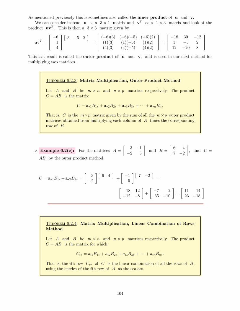
As mentioned previously this is sometimes also called the inner product of u and v.We can consider instead u as a 3 × 1 matrix and vT as a 1 × 3 matrix and look at the
product uvT . This is then a 3× 3 matrix given by
uvT =
−614
[
3 −5 2]
=
(−6)(3) (−6)(−5) (−6)(2)(1)(3) (1)(−5) (1)(2)(4)(3) (4)(−5) (4)(2)
=
−18 30 −123 −5 212 −20 8
This last result is called the outer product of u and v, and is used in our next method formultiplying two matrices.
Theorem 6.2.3: Matrix Multiplication, Outer Product Method
Let A and B be m × n and n × p matrices respectively. The productC = AB is the matrix
C = a∗1B1∗ + a∗2B2∗ + a∗3B3∗ + · · ·+ a∗nBn∗
That is, C is the m×p matrix given by the sum of all the m×p outer productmatrices obtained from multiplying each column of A times the correspondingrow of B.
⋄ Example 6.2(c): For the matrices A =
[
3 −1−2 5
]
and B =
[
6 47 −2
]
, find C =
AB by the outer product method.
C = a∗1B1∗+a∗2B2∗ =
[
3−2
][
6 4]
+
[
−15
][
7 −2]
=
[
18 12−12 −8
]
+
[
−7 235 −10
]
=
[
11 1423 −18
]
Theorem 6.2.4: Matrix Multiplication, Linear Combination of RowsMethod
Let A and B be m × n and n × p matrices respectively. The productC = AB is the matrix for which
Ci∗ = ai1B1∗ + ai2B2∗ + ai3B3∗ + · · ·+ ainBn∗.
That is, the ith row Ci∗ of C is the linear combination of all the rows of B,using the entries of the ith row of A as the scalars.
104

⋄ Example 6.2(d): For the matrices A =
[
3 −1−2 5
]
and B =
[
6 47 −2
]
, find C =
AB by the linear combination of rows method.
By the above theorem we have
C1∗ = 3[
6 4]
+ (−1)[
7 −2]
=[
18 12]
+[
−7 2]
=[
11 14]
and
C2∗ = −2[
6 4]
+ 5[
7 −2]
=[
−12 −8]
+[
35 −10]
=[
23 −18]
so
C =
[
C1∗
C2∗
]
=
[
11 1423 −18
]
Section 6.2 Exercises
1. Let A =
−5 1 −27 0 4
2 −3 6
and B =
1 2 −1−3 −7 0
5 2 3
.
(a) Find the second column of C = AB, using the linear combination of columns method,showing clearly the linear combination used and the resulting column. Label the resultusing the correct notation for the column of a matrix, as described at the beginning ofthe section.
(b) Find the product C = AB, showing the sum of outer products, the sum of resultingmatrices, and the final result.
(c) Find the third row of C = AB, using the linear combination of rows method, showingclearly the linear combination used and the resulting column. Label the result using thecorrect notation for the row of a matrix, as described at the beginning of the section.
2. Let C =
−5 1
0 4
2 −3
and D =
[
1 2
2 3
]
.
(a) Find the product A = CD, using the linear combination of rows method. Show clearlyhow each row of A is obtained, labeling each using the correct notation. Then give thefinal result A.
(b) Find the product A = CD, using the linear combination of columns method. Showclearly how each column of A is obtained, labeling each using the correct notation.Then give the final result A.
(c) Find the product A = CD using the outer product method.
105

6.3 Inverse Matrices
Performance Criteria:
6. (c) Determine whether two matrices are inverses without finding the in-verse of either.
(d) Find the inverse of a 2×2 matrix using the formula.
(e) Find the inverse of a matrix using the Gauss-Jordan method. De-scribe the Gauss-Jordan method for finding the inverse of a matrix.
Let’s begin with an example!
⋄ Example 6.3(a): Find AC and CA for the matrices A =
[
5 72 3
]
and C =
[
3 −7−2 5
]
.
AC =
[
5 72 3
] [
3 −7−2 5
]
=
[
1 00 1
]
, CA =
[
3 −7−2 5
] [
5 72 3
]
=
[
1 00 1
]
We see that AC = CA = I2.
Now let’s remember that the identity matrix is like the number one for multiplication of numbers.Note that, for example, 1
5 · 5 = 5 · 15 = 1. This is exactly what we are seeing in the above example.We say the numbers 5 and 1
5 are multiplicative inverses, and we say that the matrices A andC above are inverses of each other.
Definition 6.3.1 Inverse Matrices
Suppose that for matrices A and B we have AB = BA = I. Then we saythat A and B are inverse matrices.
Notationally we write B = A−1 or A = B−1, and we will say that A and B are invertible.Note that in order for us to be able to do both multiplications AB and BA, both matrices mustbe square and of the same dimensions. It also turns out that that to test two square matrices tosee if they are inverses we only need to multiply them in one order:
Theorem 6.3.2 Test for Inverse Matrices
To test two square matrices A and B to see if they are inverses, computeAB. If it is the identity, then the matrices are inverses.
Here a few notes about inverse matrices:
106

• Not every square matrix has an inverse, but “many” do. If a matrix does have an inverse, itis said to be invertible.
• The inverse of a matrix is unique, meaning there is only one.
• Matrix multiplication IS commutative for inverse matrices.
Two questions that should be occurring to you now are
1) How do we know whether a particular matrix has an inverse?
2) If a matrix does have an inverse, how do we find it?
There are a number of ways to answer the first question; here is one:
Theorem 6.3.3 Test for Invertibility of a Matrix
A square matrix A is invertible if, and only if, rref (A) = I.
Here is the answer to the second question in the case of a 2× 2 matrix:
Definition 6.3.4 Inverse of a 2× 2 Matrix
The inverse of a 2× 2 matrix A =
[
a b
c d
]
is A−1 =1
ad− bc
[
d −b−c a
]
.
⋄ Example 6.3(b): Find the inverse of A =
[
−2 71 −5
]
.
A−1 =1
(−2)(−5)− (1)(7)
[
−5 −7−1 −2
]
=1
3
[
−5 −7−1 −2
]
=
[
−53 −7
3
−13 −2
3
]
Before showing how to find the inverse of a larger matrix we need to go over the idea of augmentinga matrix with a vector or another matrix. To augment a matrix A with a matrix B, both matricesmust have the same number of rows. A new matrix, denoted [A | B] is formed as follows: thefirst row of [A | B] is the first row of A followed by the first row of B, and every other row in[A | B] is formed the same way.
107

⋄ Example 6.3(c): Let A =
−5 1 −27 0 4
2 −3 6
, B =
9 1
−1 8
−6 −3
and x =
−710
4
.
Give the augmented matrices [A | x] and [A | B].
[A | x] =
−5 1 −2 −77 0 4 10
2 −3 6 4
, [A | B] =
−5 1 −2 9 1
7 0 4 −1 8
2 −3 6 6 −3
Gauss-Jordan Method for Finding Inverse Matrices
Let A be an n× n invertible matrix and In be the n× n identity matrix.Form the augmented matrix [A | In] and find rref ([A | In]) = [In | B]. (Theresult of row-reduction will have this form.) Then B = A−1.
⋄ Example 6.3(d): Find the inverse of A =
2 3 0
1 −2 1
2 0 1
, if it exists.
We begin by augmenting with the 3×3 identity: [A| I3] =
2 3 0 1 0 0
1 −2 1 0 1 0
2 0 1 0 0 1
. Performing
Gauss-Jordan elimination (row reducing) then gives
1 0 0 2 3 −30 1 0 −1 −2 2
0 0 1 −4 −6 7
, so A−1 =
2 3 −3−1 −2 2
−4 −6 7
.
The above example is a bit unusual; the inverse of a randomly generated matrix will usually containfractions.
⋄ Example 6.3(e): Find the inverse of B =
1 −1 2
1 2 −10 2 −2
, if it exists.
[B | I3] =
1 −1 2 1 0 0
1 2 −1 0 1 0
0 2 −2 0 0 1
rref=⇒
1 0 1 0 1 −10 1 −1 0 0 1
2
0 0 0 1 −1 32
. Because the left
side of the reduced matrix is not the identity, the matrix B is not invertible.
108

⋄ Example 6.3(f): Find a matrix such that AB = C, where A =
[
−3 12 −1
]
and
C =
[
1 −3−2 3
]
.
Note that if we multiply both sides of AB = C on the left by A−1 we get A−1AB = A−1C.But A−1AB = B, so we have
B = A−1C =
[
−1 −1−2 −3
] [
1 −3−2 3
]
=
[
1 04 −3
]
Section 6.3 Exercises
1. Determine whether A =
[
2 5
3 8
]
and C =
[
8 −4−3 2
]
are inverses, without actually
finding the inverse of either. Show clearly how you do this.
2. Consider the matrix
[
2 3
4 5
]
.
(a) Apply row reduction (“by hand”) to [A | I2 ] until you obtain [ I2 | B ]. That is, find thereduced row-echelon form of [A | I2 ].
(b) Find AB and BA.
(c) What does this illustrate?
109

6.4 Applications of Matrices II: Rotations and Projections, Graph Theory
Performance Criteria:
6. (f) Give the geometric or algebraic representations of the inverse orsquare of a rotation. Demonstrate that the geometric and algebraicversions are the same
(g) Give the incidence matrix of a graph or digraph. Given the incidencematrix of a graph or digraph, identify the vertices and edges usingcorrect notation, and draw the graph.
(h) Determine the number of k-paths from one vertex of a graph to an-other. Solve problems using incidence matrices.
Rotation and Projection Matrices
In the Chapter 5 Exercises you should have encountered a matrix that rotated every vector inR2 thirty degrees counterclockwise, and another matrix that projected every vector in R
2 ontothe line y = 3
4x. Here are the general formulas for rotation and projection matrices in R2:
Rotation Matrix in R2
For the matrix A =
[
cos θ − sin θ
sin θ cos θ
]
and any position vector x in R2, the
product
Ax is the vector resulting when x is rotated counterclockwise around the originby the angle θ.
Projection Matrix in R2
For the matrix B =
a2
a2 + b2ab
a2 + b2
ab
a2 + b2b2
a2 + b2
and any position vector x in R2,
the
product Bx is the vector resulting when x is projected onto the line containingthe origin and the point (a, b).
In the Chapter 6 Exercises you will investigate multiplication of matrices of rotation and projectionmatrices.
110

Graphs and Digraphs
A graph is a set of dots, called vertices, connected by segments of lines or curves, callededges. An example is shown at the top left of the next page; note that a vertex can be connectedto itself. We will often label each of the vertices with a subscripted v, as shown. We can thencreate a matrix, called an incidence matrix to show which pairs of vertices are connected (andwhich are not). The (i, j) entry of the matrix is a one if vi and vj are connected by a singleedge and a zero if they are not. If i = j the entry is a one if that vertex is connected to itselfby an edge, and zero if it is not. You should be able to see this by comparing the graph and andcorresponding incidence matrix below. Note that the incidence matrix is symmetric; that is thecase for all incidence matrices of graphs.
v1
v2
v3v4
v5
0 1 1 1 01 1 1 0 01 1 0 1 11 0 1 1 10 0 1 1 0
Even though there is no edge from vertex one to vertex five for the graph shown, we can getfrom vertex one to vertex five via vertex three or vertex four. We call such a “route” a path,and we denote the paths by the sequence of vertices, like v1v3v5 or v1v4v5. These paths, inparticular, are called 2-paths, since they consist of two edges. There are other paths from vertexone to vertex five, like the 3-path v1v2v3v5 and the 4-path v1v2v2v3v5.
In some cases we want the edges of a graph to be “one-way.” We indicate this by placing anarrow on each edge, indicating the direction it goes. We will not put two arrowheads on one edge;if we can travel both ways between two vertices, we will show that by drawing TWO edges betweenthem. Such a graph is called a directed graph, or digraph for short. Below is a digraph andits incidence matrix. The (i, j) entry of the incidence matrix is one only if there is a directededge from vi to vj . Of course the incidence matrix for a digraph need not be symmetric, sincethere may be an edge going one way between two vertices but not the other way. Digraphs haveincidence matrices as well. Below is a digraph and its incidence matrix.
v1 v2
v3 v4
0 0 1 00 1 0 11 1 0 00 1 1 0
Both the graph and the digraph above are what we call connected graphs, meaning that everytwo vertices are connected by some path. All graphs that we will consider will be connected; wewill leave further discussion/investigation of graphs and incidence matrices to the exercises.
111

Section 6.4 Exercises
1. Sketch a graph with four vertices (labeled v1 - v4) and five edges (with no more than oneedge from a given vertex to another, but you can have an edge from a vertex to itself) forwhich the second row, fourth column of Ak is zero for k = 1, 2, 3, 4, ....
112

6.5 Chapter 6 Exercises
1. Let A =
−5 1
0 4
2 −3
.
(a) Give AT , the transpose of A.
(b) Find ATA and AAT . Are they the same (equal)?
(c) Your answers to (b) are special in two ways. What are they? (What I’m looking forhere is two of the special types of matrices described in Section 5.1.)
2. For the matrix A =
[
1 0 −1−3 1 2
]
, give a matrix B such that AB DOES NOT exist
(cannot be found) and a matrix C such that AC DOES exist.
3. Explain how to determine whether two matrices A and B are inverses of each other. Be sureto tell what will happen if they ARE inverses.
4. Consider the matrices A =
[
3 0 −1−1 −1 1
]
and B =
2 13 15 3
.
(a) Tell why a person might think that A and B are inverses. You should be able to do thisin a single sentence or mathematical statement.
(b) Tell why A and B are not inverses. You should be able to do this in a single sentence.
5. Show how to find the inverse of the matrix
[
2 −1−3 4
]
in the same way that you would
find the inverse of a 10× 10 matrix.
Some Trig Identities
You might find the following useful in understanding/answering some of theremaining exercises for this section.
sin2 θ + cos2 θ = 1 cos(−θ) = cos θ sin(−θ) = − sin θ
sin(2θ) = 2 sin θ cos θ cos(2θ) = cos2 θ − sin2 θ
6. Consider the general rotation matrix A =
[
cos θ − sin θ
sin θ cos θ
]
.
(a) Suppose that we were to apply A to a vector x, then apply A again, to the result.Thinking only geometrically (don’t do any calculations), give a single matrix B thatshould have the same effect.
(b) Find the matrix A2 algebraically, by multiplying A by itself.
113
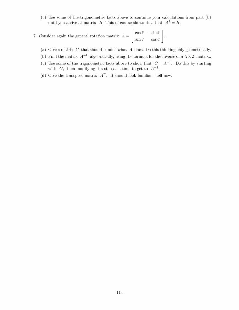
(c) Use some of the trigonometric facts above to continue your calculations from part (b)until you arrive at matrix B. This of course shows that that A2 = B.
7. Consider again the general rotation matrix A =
[
cos θ − sin θ
sin θ cos θ
]
.
(a) Give a matrix C that should “undo” what A does. Do this thinking only geometrically.
(b) Find the matrix A−1 algebraically, using the formula for the inverse of a 2×2 matrix..
(c) Use some of the trigonometric facts above to show that C = A−1. Do this by startingwith C, then modifying it a step at a time to get to A−1.
(d) Give the transpose matrix AT . It should look familiar - tell how.
114

7 Matrices and Systems of Equations
Outcome:
7. Understand the relationship of matrices with systems of equations.
Performance Criteria:
(a) Express a system of equations as a coefficient matrix times a vectorequalling another vector.
(b) Use LU -factorization to solve a system of equations, given the LU -factorization of its coefficient matrix.
(c) Solve a system of equations using an inverse matrix. Describe how touse an inverse matrix to solve a system of equations.
(d) Find the determinant of a 2×2 or 3 × 3 matrix by hand. Use acalculator to find the determinant of an n× n matrix.
(e) Use the determinant to determine whether a system of equations hasa unique solution.
(f) Know the nature of the solution to a homogenous system.
(g) Determine whether a homogeneous system has more than one solu-tion.
115

7.1 Matrix Equation Form of a System
Performance Criteria:
7. (a) Express a system of equations as a coefficient matrix times a vectorequalling another vector.
Definition 7.1.1 Matrix Equation Form of a System
A system of m linear equations in n unknowns (note that m and n need notbe equal) can be written as Ax = b where A is the m×n coefficient matrixof the system, x is the vector consisting of the n unknowns and b is thevector consisting of the m right-hand sides of the equations, as shown below.
a11x1 + · · ·+ a1nxn = b1
a21x1 + · · ·+ a2nxn = b2...
am1x1 + · · ·+ amnxn = bm
⇐⇒
a11 · · · a1n
a21 · · · a2n...
...
am1 · · · amn
x1
x2...
xn
=
b1
b2
...
bm
We will refer to this as the matrix form of a system of equations.
This form of a system of equations can be used, as you will soon see, in another method (besidesrow-reduction) for solving a system of equations. That method is occasionally useful, though notgenerally used in practice due to algorithmic inefficiency. The main benefit of this idea is thatit allows us to write a system of equations in the very compact form Ax = b that allows usto discuss both concepts and practical methods in a way that is much less cumbersome than thesystems themselves.
⋄ Example 7.1(a): Give the matrix form of the system
x1 + 3x2 − 2x3 = −43x1 + 7x2 + x3 = 4
−2x1 + x2 + 7x3 = 7
The matrix form of the system is
1 3 −23 7 1−2 1 7
x1x2x3
=
−447
We now have three interpretations of the solution (x1, x2, x3) to a system Ax = b of threeequations in three unknowns, like the one above, assuming that we have a unique solution:
1) (x1, x2, x3) is the point where the planes with the three equations intersect.
2) x1, x2 and x3 are the three scalars for a linear combination of the columns of A that equalsthe vector b.
116

3) x = [x1, x2, x3] is the vector that A transforms into the vector b.
Section 7.1 Exercises
1. Multiply
a11 a12 a13a21 a22 a23a31 a32 a33
x1x2x3
.
2. Give the matrix form Ax = b of each system of equations.
(a)
x + y − 3z = 1
−3x+ 2y − z = 7
2x+ y − 4z = 0
(b)5x − 3y + z = −4x+ y − 7z = 2
117
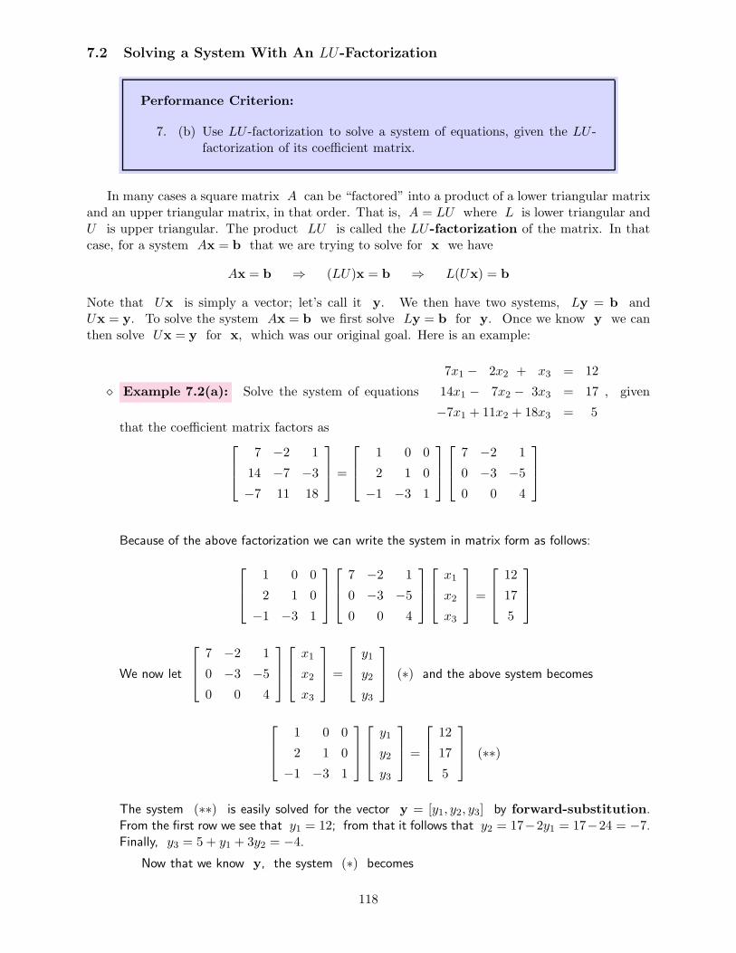
7.2 Solving a System With An LU-Factorization
Performance Criterion:
7. (b) Use LU -factorization to solve a system of equations, given the LU -factorization of its coefficient matrix.
In many cases a square matrix A can be “factored” into a product of a lower triangular matrixand an upper triangular matrix, in that order. That is, A = LU where L is lower triangular andU is upper triangular. The product LU is called the LU-factorization of the matrix. In thatcase, for a system Ax = b that we are trying to solve for x we have
Ax = b ⇒ (LU)x = b ⇒ L(Ux) = b
Note that Ux is simply a vector; let’s call it y. We then have two systems, Ly = b andUx = y. To solve the system Ax = b we first solve Ly = b for y. Once we know y we canthen solve Ux = y for x, which was our original goal. Here is an example:
⋄ Example 7.2(a): Solve the system of equations
7x1 − 2x2 + x3 = 12
14x1 − 7x2 − 3x3 = 17
−7x1 + 11x2 + 18x3 = 5
, given
that the coefficient matrix factors as
7 −2 1
14 −7 −3−7 11 18
=
1 0 0
2 1 0
−1 −3 1
7 −2 1
0 −3 −50 0 4
Because of the above factorization we can write the system in matrix form as follows:
1 0 0
2 1 0
−1 −3 1
7 −2 1
0 −3 −50 0 4
x1
x2
x3
=
12
17
5
We now let
7 −2 1
0 −3 −50 0 4
x1
x2
x3
=
y1
y2
y3
(∗) and the above system becomes
1 0 0
2 1 0
−1 −3 1
y1
y2
y3
=
12
17
5
(∗∗)
The system (∗∗) is easily solved for the vector y = [y1, y2, y3] by forward-substitution.From the first row we see that y1 = 12; from that it follows that y2 = 17−2y1 = 17−24 = −7.Finally, y3 = 5 + y1 + 3y2 = −4.
Now that we know y, the system (∗) becomes
118

7 −2 1
0 −3 −50 0 4
x1
x2
x3
=
12
−7−4
This is now solved by back-substitution. We can see that x3 = −1, so
−3x2 − 5x3 = −7 =⇒ − 3x2 + 5 = −7 =⇒ x2 = 4
Finally,7x1 − 2x2 + x3 = 12 =⇒ 7x1 − 9 = 12 =⇒ x1 = 3
The solution to the original system of equations is (3, 4,−1).
This may seem overly complicated, but the factorization of A into LU is done by rowreducing, so this method is no more costly than row-reduction in terms of operations used. Anadded benefit is that if we wish to find x for various vectors b, we do not have to row-reduce allover again each time. Here are a few additional comments about this method:
• We will see how the LU -factorization is obtained through a series of exercises.
• The LU -factorization of a matrix is not unique; that is, there are different ways to factor agiven matrix.
• LU -factorization can be done with non-square matrices, but we are not concerned with thatidea.
Section 7.2 Exercises
1. In this exercise you will be working again with the system
x1 + 3x2 − 2x3 = −43x1 + 7x2 + x3 = 4
−2x1 + x2 + 7x3 = 7
.
For the purposes of the exercise we will let
L =
1 0 03 1 0−2 −7
2 1
, U =
1 3 −20 −2 70 0 55
2
, x =
x1x2x3
, y =
y1y2y3
, b =
−447
(a) Write the system Ly = b as a system of three equations in the three unknownsy1, y2, y3. Then solve the system by hand, showing clearly how it is done. In the end,give the vector y.
(b) Write the system Ux = y as a system of three equations in the three unknownsx1, x2, x3. Then solve the system by hand, showing clearly how it is done. In the end,give the vector x.
(c) Use the linear combination of vectors interpretation of the system to show that thex1, x2, x3 you found in part (b) is a solution to the system of equations. Show the scalarmultiplication and vector addition as two separate steps.
119

(d) Multiply L times U , in that order. What do you notice about the result? If you don’tsee something, you may have gone astray somewhere!
2. Let A be the coefficient matrix for the system from the previous exercise.
(a) Give the matrix E1 be the matrix for which E1A is the result of the first row operationused to reduce A to U . Give the matrix E1A.
(b) Give the matrix E2 such that E2(E1A) is the result after the second row operationused to reduce A to U . Give the matrix E2E1A.
(c) Give the matrix E3 such that E3(E2E1A) is U .
(d) Find the matrix B = E3E2E1, then use your calculator to find B−1. What is it? Ifyou don’t recognize it, you are asleep or you did something wrong!
3. (a) Fill in the blanks of the second matrix below with the entries from E1. Then, withoutusing your calculator, fill in the blanks in the first matrix so that the product of the firsttwo matrices is the 3× 3 identity, as shown.
=
1 0 0
0 1 0
0 0 1
Call the matrix you found F1. Do the same thing with E2 and E3 to find matricesF2 and F3.
(b) Find the product F1F2F3, in that order. Again, you should recognize the result.
120

7.3 Inverse Matrices and Systems
Performance Criterion:
7. (c) Solve a system of equations using an inverse matrix. Describe how touse an inverse matrix to solve a system of equations.
Let’s consider a simple algebraic equation of the form ax = b, where a and b are justconstants. If we multiply both sides on the left by 1
a, the multiplicative inverse of a, we get
x = 1a· b. for example,
3x = 5
13 (3x) = 1
3 · 5(
13 · 3
)
x = 53
1x = 53
x = 53
The following shows how an inverse matrix can be used to solve a system of equations by exactlythe same idea:
Ax = b
A−1(Ax) = A−1 b
(A−1A)x = A−1 b
Ix = A−1 b
x = A−1 b
Note that this only “works” if A is invertible! The upshot of all this is that when A is invertiblethe solution to the system Ax = b is given by x = A−1 b. The above sequence of steps showsthe details of why this is. Although this may seem more straightforward than row reduction, it ismore costly in terms of computer time than row reduction or LU -factorization. Therefore it is notused in practice.
⋄ Example 7.3(a): Solve the system of equations5x1 + 4x2 = 25
−2x1 − 2x2 = −12using an inverse
matrix, showing all steps given above.
The matrix form of the system is
[
5 4
−2 −2
][
x1
x2
]
=
[
25
−12
]
, and A−1 = −12
[
−2 −42 −5
]
.
A−1 can now be used to solve the system:
[
5 4
−2 −2
][
x1
x2
]
=
[
25
−12
]
−1
2
[
−2 −42 −5
]([
5 4
−2 −2
][
x1
x2
])
= −1
2
[
−2 −42 −5
][
25
−12
]
121

(
−1
2
[
−2 −42 −5
] [
5 4
−2 −2
])[
x1
x2
]
= −1
2
[
−2−10
]
[
1 0
0 1
][
x1
x2
]
=
[
1
5
]
[
x1
x2
]
=
[
1
5
]
The solution to the system is (1, 5).
Section 7.3 Exercises
1. Assume that you have a system of equations Ax = b for some invertible matrix A. Showhow the inverse matrix is used to solve the system, showing all steps in the process clearly.Check your answer against what is shown in Section 7.3.
2. Consider the system of equations2x1 − 3x2 = 4
4x1 + 5x2 = 3.
(a) Write the system in matrix times a vector form Ax = b.
(b) Apply the formula in Section 6.2 to obtain the inverse matrix A−1. Show a step ortwo in how you do this.
(c) Demonstrate that your answer to (b) really is the inverse of A.
(d) Use the inverse matrix to solve the system. Show ALL steps outlined in Section7.3, and give your answer in exact form.
(e) Apply row reduction (“by hand”) to [A | I2 ] until you obtain [ I2 | B ]. That is,find the reduced row-echelon form of [A | I2 ]. What do you notice about B?
3. Consider the system of equations5x+ 7y = −12x+ 3y = 4
(a) Write the system in Ax = b form.
(b) Use the formula for the inverse of a 2× 2 matrix to find A−1.
(c) Give the matrix that is to be row reduced to find A−1 by the Gauss-Jordan method.Then give the reduced row-echelon form obtained using your calculator.
(d) Repeat EVERY step of the process for solving Ax = b using the inverse matrix. SeeSection 7.3 for all the steps.
122

7.4 Determinants and Matrix Form
Performance Criterion:
7. (d) Find the determinant of a 2×2 or 3 × 3 matrix by hand. Use acalculator to find the determinant of an n× n matrix.
(e) Use the determinant to determine whether a system of equations hasa unique solution.
Associated with every square matrix is a scalar that is called the determinant of the matrix,and determinants have numerous conceptual and practical uses. For a square matrix A, the deter-minant is denoted by det(A). This notation implies that the determinant is a function that takes a
matrix returns a scalar. Another notation is that the determinant of a specific matrix
[
a b
c d
]
is
denoted by det
[
a b
c d
]
or
∣
∣
∣
∣
a b
c d
∣
∣
∣
∣
.
There is a simple formula for finding the determinant of a 2× 2 matrix:
Definition 7.4.1: Determinant of a 2× 2 Matrix
The determinant of the matrix
[
a b
c d
]
is det(A) = ad− bc.
⋄ Example 7.4(a): Find the determinant of A =
[
5 4
−2 −2
]
det(A) = (5)(−2) − (−2)(4) = −10 + 8 = −2
There is a fairly involved method of breaking the determinant of a larger matrix down to whereit is a linear combination of determinants of 2× 2 matrices, but we will not go into that here. Itis called the cofactor expansion of the determinant, and can be found in most any other linearalgebra book, or online. Of course your calculator will find determinants of matrices whose entriesare numbers,as will online matrix calculators and various software like MATLAB.
Later we will need to be able to find determinants of matrices containing an unknown parameter,and it will be necessary to find determinants of 3 × 3 matrices. For that reason, we now show arelatively simple method for finding the determinant of a 3× 3 matrix. (This will not look simplehere, but it is once you are familiar with it.) This method only works for 3× 3 matrices.
123
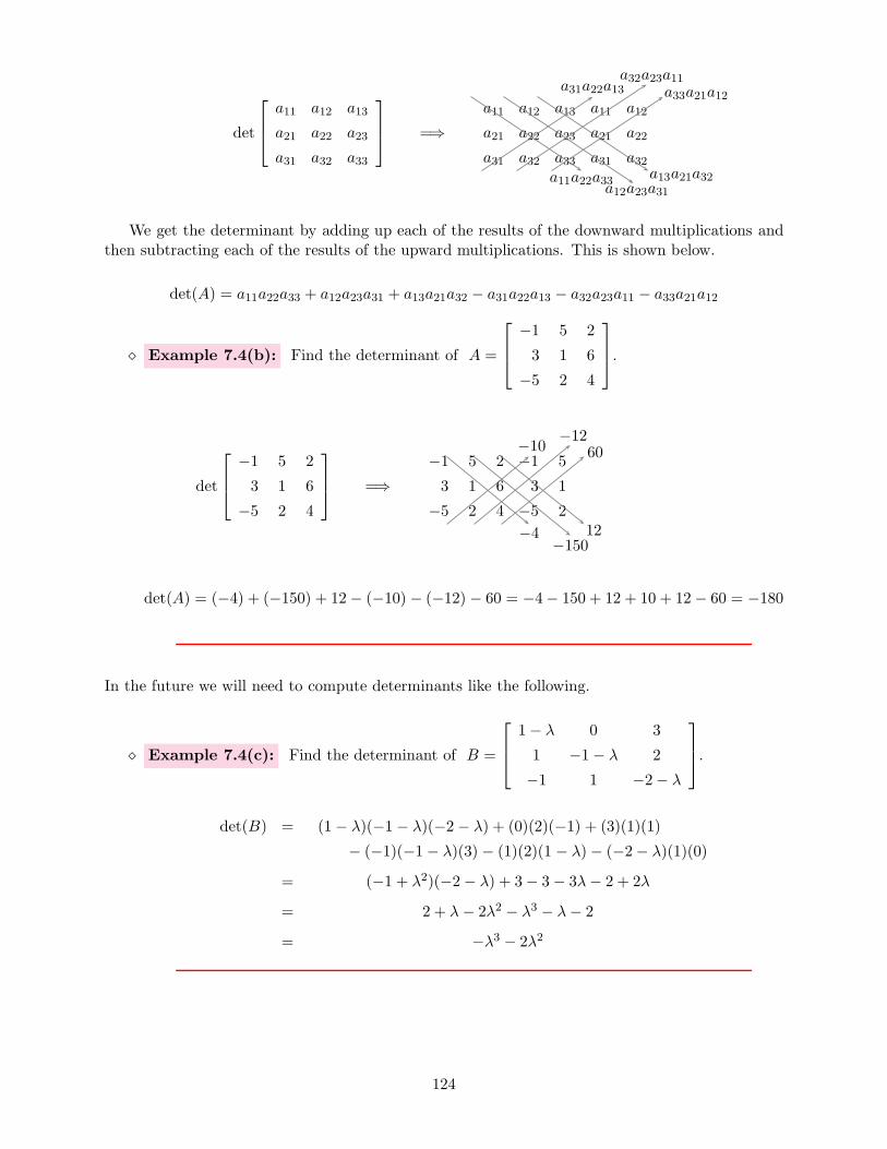
det
a11 a12 a13
a21 a22 a23
a31 a32 a33
=⇒
a11 a12 a13 a11 a12
a21 a22 a23 a21 a22
a31 a32 a33 a31 a32a11a22a33
a12a23a31a13a21a32
a31a22a13a32a23a11
a33a21a12
We get the determinant by adding up each of the results of the downward multiplications andthen subtracting each of the results of the upward multiplications. This is shown below.
det(A) = a11a22a33 + a12a23a31 + a13a21a32 − a31a22a13 − a32a23a11 − a33a21a12
⋄ Example 7.4(b): Find the determinant of A =
−1 5 2
3 1 6
−5 2 4
.
det
−1 5 2
3 1 6
−5 2 4
=⇒
−1 5 2 −1 5
3 1 6 3 1
−5 2 4 −5 2
−4−150
12
−10 −1260
det(A) = (−4) + (−150) + 12− (−10) − (−12) − 60 = −4− 150 + 12 + 10 + 12− 60 = −180
In the future we will need to compute determinants like the following.
⋄ Example 7.4(c): Find the determinant of B =
1− λ 0 3
1 −1− λ 2
−1 1 −2− λ
.
det(B) = (1− λ)(−1− λ)(−2− λ) + (0)(2)(−1) + (3)(1)(1)
− (−1)(−1− λ)(3) − (1)(2)(1 − λ)− (−2− λ)(1)(0)
= (−1 + λ2)(−2− λ) + 3− 3− 3λ− 2 + 2λ
= 2 + λ− 2λ2 − λ3 − λ− 2
= −λ3 − 2λ2
124

Here is why we care about determinants right now:
Theorem 7.4.2: Determinants and Invertibility, Systems
Let A be a square matrix.
(a) A is invertible if, and only if, det(A) 6= 0.
(b) The system Ax = b has a unique solution if, and only if, A is invertible.
(c) If A is not invertible, the system Ax = b will have either no solutionor infinitely many solutions.
Recall that when things are “nice” the system Ax = b can be solved as follows:
Ax = b
A−1(Ax) = A−1 b
(A−1A)x = A−1 b
Ix = A−1 b
x = A−1 b
In this case the system will have the unique solution x = A−1 b. (When we say unique, we meanonly one.) If A is not invertible, the above process cannot be carried out, and the system willnot have a single unique solution. In that case there will either be no solution or infinitely manysolutions.
We previously discussed the fact that the above computation is analogous to the following onesinvolving simple numbers and an unknown number x:
3x = 5
13 (3x) = 1
3 · 5(
13 · 3
)
x = 53
1x = 53
x = 53
Now let’s consider the following two equations, of the same form ax = b but for which a = 0:
0x = 5 0x = 0
We first recognize that we can’t do as before and multiply both sides of each by 10 , since that is
undefined. The first equation has no solution, since there is no number x that can be multiplied byzero and result in five! In the second case, every number is a solution, so the system has infinitelymany solutions. These equations are analogous to Ax = b when det(A) = 0. The one differenceis that Ax = b can have infinitely many solutions even when b is NOT the zero vector.
125

Section 7.4 Exercises
1. Explain/show how to use the determinant to determine whether
x+ 3y − 3z = −52x− y + z = −3
−6x+ 3y − 3z = 4
has a unique solution. You may use your calculator for finding determinants - besure to conclude by saying whether or not this particular system has a solution!
2. Suppose that you hope to solve a system Ax = b of n equations in n unknowns.
(a) If the determinant of A is zero, what does it tell you about the nature of the solution?(By “the nature of the solution” I mean no solution, a unique solution or infinitely manysolutions.)
(b) If the determinant of A is NOT zero, what does it tell you about the nature of thesolution?
3. Suppose that you hope to solve a system Ax = 0 of n equations in n unknowns.
(a) If the determinant of A is zero, what does it tell you about the nature of the solution?(By “the nature of the solution” I mean no solution, a unique solution or infinitely manysolutions.)
(b) If the determinant of A is NOT zero, what does it tell you about the nature of thesolution?
126

7.5 Homogeneous Systems
Performance Criterion:
7. (f) Know the nature of the solution to a homogenous system.
(g) Determine whether a homogeneous system has more than one solu-tion.
Homogenous systems are important and will come up in a couple places in the future, but thereis not a whole lot that can be said about them! A homogenous system is one of the form Ax = 0.With a tiny bit of thought this should be clear: Every homogenous system has at least one solution- the zero vector! Given the results from the previous section, if A is invertible (so det(A) 6= 0),that is the only solution. If A is not invertible there will be infinitely many solutions, the zerovector being just one of them.
127

7.6 Chapter 7 Exercises
1. Consider the system3x+ 2y = −14x+ 5y = 1
. The inverse of
[
3 24 5
]
is1
7
[
5 −2−4 3
]
. Use
the inverse to solve the system of equations, showing all steps in the process clearly.
2. Suppose that we are trying to solve the system of equationsx1 + 3x2 = −4
5x1 − 2x2 = 5. One
geometric interpretation of this problem is “Find the point in R2 where the two lines
x1+3x2 = −4 and 5x1−2x2 = 5 intersect.” Two other interpretations follow; fill the emptyspaces in each with specific vectors or matrices.
(a) Find a linear combination of the two vectors and that equals .
(b) Find a vector that when multiplied by the matrix results in .
128

8 Vector Spaces and Subspaces
Outcome:
8. Understand subspaces of Rn. Find a least squares solution to an incon-
sistent system of equations.
Performance Criteria:
(a) Describe the span of a set of vectors in R2 or R
3 as a line or planecontaining a given set of points.
(b) Determine whether a vector w is in the span of a set v1,v2, ...,vkof vectors. If it is, write w as a linear combination of v1,v2, ...,vk.
(c) Determine whether a set is closed under an operation. If it is, provethat it is; if it is not, give a counterexample.
(d) Determine whether a subset of Rn is a subspace. If so, prove it; ifnot, give an appropriate counterexample.
(e) Determine whether a vector is in the column space or null space of amatrix, based only on the definitions of those spaces.
(f) Find the least-squares approximation to the solution of an inconsis-tent system of equations. Solve a problem using least-squares approx-imation.
(g) Give the least squares error and least squares error vector for a leastsquares approximation to a solution to a system of equations.
129

8.1 Span of a Set of Vectors
Performance Criteria:
8. (a) Describe the span of a set of vectors in R2 or R
3 as a line or planecontaining a given set of points.
(b) Determine whether a vector w is in the span of a set v1,v2, ...,vkof vectors. If it is, write w as a linear combination of v1,v2, ...,vk.
Definition 8.1.1: The span of a set S of vectors, denoted span(S) isthe set of all linear combinations of those vectors.
⋄ Example 8.1(a): Describe the span of the set S =
100
,
010
in R3.
Note that ANY vector with a zero third component can bewritten as a linear combination of these two vectors:
a
b
0
= a
100
+ b
010
All the vectors with x3 = 0 (or z = 0) are the xy plane in R3,
so the span of this set is the xy plane. Geometrically we cansee the same thing in the picture to the right.
010
100
a
b
0
x
y
z
⋄ Example 8.1(b): Describe span
1−20
,
310
.
By definition, the span of this set is all vectors v of the form
v = c1
1
−20
+ c2
3
1
0
,
which, because the two vectors are not scalar multiples of each other, we recognize as being aplane through the origin. It should be clear that all vectors created by such a linear combination
130

will have a third component of zero, so the particular plane that is the span of the two vectors isthe xy-plane. Algebraically we see that any vector [a, b, 0] in the xy-plane can be created by
(
a− 3b
7
)
1
−20
+
(
2a+ b
7
)
3
1
0
=
a−3b7
−2a+6b7
0
+
6a+3b7
2a+b7
0
=
7a77b7
0
=
a
b
0
You might wonder how one would determine the scalars a−3b7 and 2a+b
7 . You will see how this isdone in the exercises!
At this point we should make a comment and a couple observations:
• First, some language: we can say that the span of the two vectors in Example 8.1(b) is thexy-plane, but we also say that the two vectors span the xy-plane. That is, the word span canbe used as either a noun or a verb, depending on how it is used.
• Note that in the two examples above we considered two different sets of two vectors, but ineach case the span was the same. This illustrates that different sets of vectors can have thesame span.
• Consider also the fact that if we were to include in either of the two sets additional vectorsthat are also in the xy-plane, it would not change the span. However, if we were to addanother vector not in the xy-plane, the span would increase to all of R
3.
• In either of the preceding examples, removing either of the two given vectors would reducethe span to a linear combination of a single vector, which is a line rather than a plane. Butin some cases, removing a vector from a set does not change its span.
• The last two bullet items tell us that adding or removing vectors from a set of vectors mayor may not change its span. This is a somewhat undesirable situation that we will remedy inthe next chapter.
• It may be obvious, but it is worth emphasizing that (in this course) we will consider spansof finite (and usually rather small) sets of vectors, but a span itself always contains infinitelymany vectors (unless the set S consists of only the zero vector).
It is often of interest to know whether a particular vector is in the span of a certain set of vectors.The next examples show how we do this.
⋄ Example 8.1(c): Is v =
3−2−41
in the span of S =
1234
,
1−11−1
,
20−31
?
The question is, “can we find scalars c1, c2 and c3 such that
c1
1234
+ c2
1−11−1
+ c3
20−31
=
3−2−41
?” (1)
131

We should recognize this as the linear combination form of the system of equations below and tothe left. The augmented matrix for the system row reduces to the matrix below and to the right.
c1 + c2 + 2c3 = 3
2c1 − c2 = −23c1 + c2 − 3c3 = −44c1 − c2 + c3 = 1
1 0 0 00 1 0 00 0 1 00 0 0 1
This tells us that the system above and to the left has no solution, so there are no scalars c1,c2 and c3 for which equation (1) holds. Thus v is not in the span of S.
⋄ Example 8.1(d): Is v =
1910−1
in span(S), where S =
3−12
,
−501
,
17−4
?
Here we are trying to find scalars c1, c2 and c3 such that
c1
3−12
+ c2
−501
+ c3
17−4
=
1910−1
(2)
We should recognize this as the linear combination form of the system of equations below and tothe left. The augmented matrix for the system row reduces to the matrix below and to the right.
3c1 − 5c2 + c3 = 19
−c1 + 7c3 = 10
2c1 + c2 − 4c3 = −1
1 0 0 40 1 0 −10 0 1 2
This tells us that (2) holds for c1 = 4, c2 = −1 and c3 = 2, so v is in span(S).
Sometimes, with a little thought, no computations are necessary to answer such questions, as thenext examples show.
⋄ Example 8.1(e): Is v =
−425
in the span of S =
−302
,
−501
?
One can see that any linear combination of the two vectors in S will have zero as its secondcomponent:
c1
−302
+ c2
−501
=
−3c102c1
+
−5c201c2
=
−3c1 − 5c20
2c1 + c2
Since the second component of v is not zero, v is not in the span of the set S.
132
⋄ Example 8.1(f): Is v =
47−1
in span
100
,
010
,
001
?
Here we can see that if we multiply the three vectors in S by 4, 7 and −1, respectively, andadd them, the result will be v:
4
100
+ 7
010
− 1
001
=
400
+
070
+
00−1
=
47−1
Therefore v is in span
100
,
010
,
001
.
Sometimes we will be given an infinite set of vectors, and we’ll ask whether a particular finiteset of vectors spans the infinite set. By this we are asking whether the span of the finite set is the
infinite set. For example, we might ask whether the vector v =
[
23
]
spans R2. Because the
span of the single vector v is just a line, v does not span R2. With the knowledge we have
at this point, it can sometimes be difficult to tell whether a finite set of vectors spans a particularinfinite set. The next chapter will give us a means for making such a judgement a bit easier.
We conclude with a few more observations. With a little thought, the following can be seen tobe true. (Assume all vectors are non-zero.)
• The span of a single vector is all scalar multiples of that vector. In R2 or R
3 the span ofa single vector is a line through the origin.
• The span of a set of two non-parallel vectors in R2 is all of R
2. In R3 it is a plane through
the origin.
• The span of three vectors in R3 that do not lie in the same plane is all of R
3.
Section 8.1 Exercises
1. Describe the span of each set of vectors in R2 or R
3 by telling what it is geometrically and,if it is a standard set like one of the coordinate axes or planes, specifically what it is. If it isa line that is not one of the axes, give two points on the line. If it is a plane that is not oneof the coordinate planes, give three points on the plane.
(a) The vector
[
50
]
in R2.
(b) The set of vectors
501
,
003
in R3.
(c) The vectors
[
51
]
and
[
03
]
in R2.
(d) The set
000
in R3.
133

(e) The vectors
123
and
246
in R3.
2. For each of the following, determine whether the vector w is in the span of the set S. Ifit is, write it as a linear combination of the vectors in S.
(a) w =
−254
, S =
3−14
,
427
,
3−11−1
(b) w =
−5−23128
, S =
1−4−37
,
26−45
(c) w =
838−1411
, S =
1−4−37
,
26−45
(d) w =
37−4
, S =
100
,
110
,
111
134

8.2 Closure of a Set Under an Operation
Performance Criteria:
8. (c) Determine whether a set is closed under an operation. If it is, provethat it is; if it is not, give a counterexample.
Consider the set 0, 1, 2, 3, ..., which are called the whole numbers. Notice that if we addor multiply any two whole numbers the result is also a whole number, but if we try subtractingtwo such numbers it is possible to get a number that is not in the set. We say that the wholenumbers are closed under addition and multiplication, but the set of whole numbers is notclosed under subtraction. If we enlarge our set to be the integers ...,−3,−2,−1, 0, 1, 2, 3, ... weget a set that is closed under addition, subtraction and multiplication. These operations we areconsidering are called binary operations because they take two elements of the set and create asingle new element. An operation that takes just one element of the set and gives another (possiblythe same) element of the set is called a unary operation. An example would be absolute value;note that the set of integers is closed under absolute value.
Definition 8.2.1: Closed Under an Operation
A set S is said to be closed under a binary operation ∗ if for every s andt in S, s ∗ t is in S. S is closed under a unary operation 〈 〉 if for everys in S, 〈s〉 is in S.
Notice that the term “closed,” as defined here, only makes sense in the context of a set with anoperation. Notice also that it is the set that is closed, not the operation. The operation is importantas well; as we have seen, a given set can be closed under one operation but not another.
When considering closure of a set S under a binary operation ∗, our considerations are asfollows:
• We first wish to determine whether we think S IS closed under ∗.
• If we do think that S is closed under ∗, we then need to prove that it is. To do this, weneed to take two general, or arbitrary elements x and y of S and show that x ∗ y is inS.
• If we think that S is not closed under ∗, we need to take two specific elements x andy of S and show that x ∗ y is not in S.
⋄ Example 8.2(a): The odd integers are the numbers ...,−5,−3,−1, 1, 3, 5, .... Are the oddintegers closed under addition? Multiplication?
We see that 3 + 5 = 8. Because 3 and 5 are both odd but their sum isn’t, the odd integersare not closed under addition. Let’s try multiplying some odds:
3× 5 = 15 − 7× 9 = −63 − 1×−7 = 7
135

Based on these three examples, it appears that the odd integers are perhaps closed under mul-tiplication. Let’s attempt to prove it. First we observe that any number of the form 2n + 1,where n is any integer, is odd. (This is in fact the definition of an odd integer.) So if we havetwo possibly different odd integers, we can write them as 2m+ 1 and 2n+ 1, where m andn are not necessarily the same integers. Their product is
(2m+ 1)(2n + 1) = 4mn+ 2m+ 2n+ 1 = 2(2mn+m+ n) + 1.
Because the integers are closed under multiplication and addition, 2mn +m + n is an integerand the product of 2m+ 1 and 2n + 1 is of the form two times an integer, plus one, so it isodd as well. Therefore the odd integers are closed under multiplication.
Closure of a set under an operation is a fairly general concept; let’s narrow our focus to whatis important to us in linear algebra.
⋄ Example 8.2(b): Prove that then span of a set S = v1,v2,v3, ...,vk in Rn is closed
under addition and scalar multiplication.
Suppose that u and w are in span(S). Then there are scalars c1, c2, c3, ..., ck andd1, d2, d3, ..., dk such that
u = c1v1 + c2v2 + c3v3 + · · · + ckvk and w = d1v1 + d2v2 + d3v3 + · · ·+ dkvk.
Therefore
u+w = (c1v1 + c2v2 + c3v3 + · · ·+ ckvk) + (d1v1 + d2v2 + d3v3 + · · · + dkvk)
= (c1 + d1)v1 + (c2 + d2)v2 + (c3 + d3)v3 + · · · + (ck + dk)vk
This last expression is a linear combination of the vectors in S, so it is in span(S). Thereforespan(S) is closed under addition. Now suppose that u is as above and a is any scalar. Then
au = a(c1v1 + c2v2 + c3v3 + · · · + ckvk)
= ac1v1 + ac2v2 + ac3v3 + · · · + ackvk
which is also a linear combination of the vectors in S, so it is also in span(S). Thus span(S) isclosed under multiplication by scalars.
The result of the above Example is that
Theorem 8.2.2: The span of a set S of vectors is closed under vector additionand scalar multiplication.
This seemingly simple observation is the beginning of one of the most important stories in thesubject of linear algebra. The remainder of this chapter and all of the next will fill out the rest ofthat story.
136

8.3 Vector Spaces and Subspaces
Performance Criterion:
8. (d) Determine whether a subset of Rn is a subspace. If so, prove it; if
not, give an appropriate counterexample.
Vector Spaces
The term “space” in math simply means a set of objects with some additional special properties.There are metric spaces, function space, topological spaces, Banach spaces, and more. The vectorsthat we have been dealing with make up the vector spaces called R
2, R3 and, for larger values,
Rn. In general, a vector space is simply a collection of objects called vectors (and a set of scalars)
that satisfy certain properties.
Definition 8.3.1: Vector Space
A vector space is a set V of objects called vectors and a set of scalars(usually the real numbers R), with the operations of vector addition and scalarmultiplication, for which the following properties hold for all u, v, w inV and scalars c and d.
1. u+ v is in V
2. u+ v = v + u
3. (u+ v) +w = u+ (v +w)
4. There exists a vector 0 in V such that u+0 = u. This vector is calledthe zero vector.
5. For every u in V there exists a vector −u in V such that u+(−u) = 0.
6. cu is in V .
7. c(u+ v) = cu+ cv
8. (c+ d)u = cu+ du
9. c(du) = (cd)u
10. 1u = u
Note that items 1 and 6 of the above definition say that the vector space V is closed under additionand scalar multiplication.
When working with vector spaces, we will be very interested in certain subsets of those vectorspaces that are the span of a set of vectors. As you proceed, recall Example 8.2(b), where weshowed that the span of a set of vectors is closed under addition and scalar multiplication.
137

Subspaces of Vector Spaces
As you should know by now, the two main operations with vectors are multiplication by scalarsand addition of vectors. (Note that these two combined give us linear combinations, the foundationof almost everything we’ve done.) A given vector space can have all sorts of subsets; consider thefollowing subsets of R
2.
• The set S1 consisting of the first quadrant and the nonnegative parts of the two axes, or all
vectors of the form
[
x1x2
]
such that x1 ≥ 0 and x2 ≥ 0.
• The set S2 consisting of the line containing the vector
[
32
]
. Algebraically this is all
vectors of the form t
[
32
]
where t ranges over all real numbers.
• The set S3 consisting of the first and third quadrants and both axes. This can be described
as the set of all vectors
[
x1x2
]
with x1x2 ≥ 0.
Our current concern is whether these subsets of R2 are closed under addition and scalar multi-
plication. With a bit of thought you should see that S1 is closed under addition, but not scalarmultiplication when the scalar is negative:
u
v
u+ vS1
w
cwc < 0
S1
In some sense we can solve the problem of not being closed under scalar multiplication by includingthe third quadrant as well to get S3, but then the set isn’t closed under addition:
w
cwc < 0
S3
S3
u
vu+ v
S3
S3
Finally, the set S2 is closed under both addition and scalar multiplication. That is a bit messy
to show with a diagram, but consider the following. S2 is the span of the single vector
[
32
]
,
and we showed in the last section that the span of any set of vectors is closed under addition andscalar multiplication.
It turns out that when working with vector spaces the only subsets of any real interest are theones that are closed under both addition and scalar multiplication. We give such subsets a name:
138

Definition 8.3.2: Subspace of Rn
A subset S of Rn is called a subspace of R
n if for every scalar c and anyvectors u and v in S, cu and u+ v are also in S. That is, S is closedunder scalar multiplication and addition.
You will be asked whether certain subsets of R2, R
3 or Rn are subspaces, and it is your job
to back your answers up with some reasoning. This is done as follows:
• When a subset IS a subspace a general proof is required. That is, we must show that the setis closed under scalar multiplication and addition, for ALL scalars and ALL vectors. We mayhave to do this outright, but if it is clear that the set of vectors is the span of some set ofvectors, then we know from the argument presented in Example 8.2(b) that the set is closedunder addition and scalar multiplication, so it is a subspace.
• When a subset IS NOT a subspace, we demonstrate that fact with a SPECIFIC example.Such an example is called a counterexample. Notice that all we need to do to show that asubset is not a subspace is to show that that it is not closed under scalar multiplication ORvector addition. If either is the case, then the set in question is not a subspace. Even if bothare the case, we need only show one.
The following examples illustrate these things.
⋄ Example 8.3(a): Show that the set S1 consisting of all vectors of the form
[
x1x2
]
such
that x1 ≥ 0 and x2 ≥ 0 is not a subspace of R2.
As mentioned before, this set is not closed under multiplication by negative scalars, so we just
need to give a specific example of this. Let u =
[
35
]
and c = −2. Clearly u is in S1 and
cu = (−2)[
35
]
=
[
−6−10
]
, which is not in S1. Therefore S1 is not closed under scalar
multiplication so it is not a subspace of R2.
⋄ Example 8.3(b): Show that the set S2 consisting of all vectors of the form t
[
32
]
,
where t ranges over all real numbers, is a subspace of R2.
Let c be any scalar and let u = s
[
32
]
and v = t
[
32
]
. Then u and v are both in
S2 and
cu = c
(
s
[
32
])
= (cs)
[
32
]
and u+ v = s
[
32
]
+ t
[
32
]
= (s+ t)
[
32
]
.
Because cs and s+ t are scalars, we can see that both cu and u+ v are in S2, so S2 isa subspace of R
2.
139

This last example demonstrates the general method for showing that a set of vectors is closed underaddition and scalar multiplication. That said, the given subspace could have been shown to be s
subspace by simply observing that it is the span of the set consisting of the single vector
[
32
]
.
From Theorem 8.2.2 we know that the span of any set of vectors is a subspace, so the set describedin the above example is a subspace of R
2.
⋄ Example 8.3(c): Determine whether the subset S of R3 consisting of all vectors of
the form x =
25−1
+ t
4−13
is a subspace. If it is, prove it. If it is not, provide a
counterexample.
We recognize this as a line in R3 passing through the point (2, 5,−1),
and it is not hard to show that the line does not pass through the origin.Remember that what we mean by the line is really all position vectors(so with tails at the origin) whose tips are on the line. Considering asimilar situation in R
2, we see that u is such a vector for the linel shown. It should be clear that if we multiply u by any scalar otherthan one, the resulting vector’s tip will not lie on the line. Thus wewould guess that the set S, even though it is in R
3, is probably notclosed under scalar multiplication.
u
l
Now let’s prove that it isn’t. To do this we first let u =
25−1
+ 1
4−13
=
642
, which
is in S. Let c = 2, so 2u =
1284
. We need to show that this vector is not in S. If it
were, there would have to be a scalar t such that
1284
=
25−1
+ t
4−13
. Subtracting
25−1
we get
1035
= t
4−13
. We can see that the value of t that would be needed
to give the correct second component would be −3, but this would result in a third component
of −9, which is not correct. Thus there is no such t and the vector
1284
is not in S.
Thus S is not closed under scalar multiplication, so it is not a subspace of R3.
We should compare the results of Examples 8.3(b) and 8.3(c). Note that both are lines in theirrespective R
n’s, but the line in 8.3(b) passes through the origin, and the one in 8.3(c) does not. Itis no coincidence that the set in 8.3(b) is a subspace and the set in 8.3(c) is not. If a set S is asubspace, being closed under scalar multiplication means that zero times any vector in the subspacemust also be in the subspace. But zero times a vector is the zero vector 0. Therefore
140

Theorem 8.3.3: Subspaces Contain the Zero Vector
If a subset S of Rn is a subspace, then the zero vector is in S.
This type of a statement is called a conditional statement. Related to any conditional statementare two other statements called the converse and contrapositive of the conditional statement.In this case we have
• Converse: If the zero vector is in a subset S of Rn, then S is a subspace.
• Contrapositive: If the zero vector is not in a subset S of Rn, then S is not a subspace.
When a conditional statement is true, its converse may or may not be true. In this case the converseis not true. This is easily seen in Example 8.3(a), where the set contains the zero vector but isnot a subspace. However, when a conditional statement is true, its contrapositive is true as well.Therefore the second statement above is the most useful of the three statements, since it gives us aquick way to rule out a set as a subspace. In Example 8.3(c) this would have saved us the troubleof providing a counterexample, although we’d still need to convincingly show that the zero vectoris not in the set.
⋄ Example 8.3(d): Determine whether the set of all vectors of the form x =
a
a+ b
b
a− b
,
for some real numbers a and b, is a subspace of R4.
We first note that a vector x of the given form will be the zero vector if a = b = 0. By theprevious discussion we cannot then rule out the possibility that the given set is a subspace, butneither do we yet know it IS a subspace. But we observe that
x =
a
a+ b
b
a− b
=
a
a
0a
+
0b
b
−b
= a
1101
+ b
011−1
.
Thus the set of vectors under consideration is the span of S =
1101
,
011−1
, so it is a
subspace.
We conclude this section with an example that gives us the “largest” and “smallest” subspacesof R
n.
⋄ Example 8.3(e): Of course a scalar times any vector in Rn is also in R
n, and the sumof any two vectors in R
n is in Rn, so R
n is a subspace of itself. Also, the zero vector byitself is a subspace of R
n as well, often called the trivial subspace.
141

At this point we have seen a variety of subspaces, and some sets that are not subspaces aswell. From Example 8.2(b) we know that the span of two linearly independent vectors in R
3 isa subspace of R
3. But we know that the span of two linearly independent vectors in R3 is a
plane through the origin. Note that we could impose a coordinate system on any plane to makeit essentially R
2, so we can think of this particular variety of subspace as just being a copy ofR2 sitting inside R
3. This illustrates what is in fact a general principle: any subspace of Rn is
essentially a copy of Rm, for some m ≤ n, sitting inside R
n with its origin at the origin of Rn.
More formally we have the following:
Subspaces of Rn
• The only non-trivial subspaces of R2 are lines through the origin and all
of R2.
• The only non-trivial subspaces of R3 are lines through the origin, planes
through the origin, and all of R3.
• The only non-trivial subspaces of Rn are hyperplanes (including lines)
through the origin and all of Rn.
Section 8.3 Exercises
1. For each of the following subsets of R3, think of each point as a position vector; each set thenbecomes a set of vectors rather than points. For each,
• determine whether the set is a subspace and
• if it is NOT a subspace, give a reason why it isn’t by doing one of the following:
⋄ stating that the set does not contain the zero vector
⋄ giving a vector that is in the set and a scalar multiple that isn’t (show that it isn’t)
⋄ giving two vectors that in the set and showing that their sum is not in the set
(a) All points on the horizontal plane at z = 3.
(b) All points on the xz-plane.
(c) All points on the line containing u = [−3, 1, 4].
(d) All points on the lines containing u = [−3, 1, 4] and v = [5, 0, 2].
(e) All points for which x ≥ 0, y ≥ 0 and z ≥ 0.
(f) All points x given by x = w + su+ tv, where w = [1, 1, 1] and u and v are as in (d).
(g) All points x given by x = su+ tv, where u and v are as in (d).
(h) The vector 0.
(i) All of R3.
142

2. Consider the vectors u =
8−24
, v =
701
and w =
−164−8
.
(a) Is the set of all vectors x = u+ tv, where t ranges over all real numbers, a subspace ofR3? If not, tell why not.
(b) Is the set of all vectors x = u+ tw, where t ranges over all real numbers, a subspace ofR3? If not, tell why not.
143

8.4 Column Space and Null Space of a Matrix
Performance Criteria:
8. (e) Determine whether a vector is in the column space or null space of amatrix, based only on the definitions of those spaces.
In this section we will define two important subspaces associated with a matrix A, its columnspace and its null space.
Definition 8.4.1: Column Space of a Matrix
The column space of an m× n matrix A is the span of the columns of A.It is a subspace of R
m and we denote it by col(A).
⋄ Example 8.4(a): Determine whether u =
338
and v =
−251
are in the column space
of A =
2 5 1−1 −7 −53 4 −2
.
We need to solve the two vector equations of the form
c1
2−13
+ c2
5−74
+ c3
1−5−2
= b, (1)
with b first being u, then v. The respective reduced row-echelon forms of the augmented matricescorresponding to the two systems are
1 0 −2 40 1 1 −10 0 0 0
and
1 0 −2 00 1 1 00 0 0 1
Therefore we can find scalars c1, c2 and c3 for which (1) holds when b = u, but not whenb = v. From this we deduce that u is in col(A), but v is not.
Recall that the system Ax = b of m linear equations in n unknowns can be written inlinear combination form:
x1
a11
a21
...
am1
+ x2
a12
a22
...
am2
+ · · ·+ xn
a1n
a2n
...
amn
=
b1
b2
...
bn
144

Note that the left side of this equation is simply a linear combination of the columns of A, withthe scalars being the components of x. The system will have a solution if, and only if, b can bewritten as a linear combination of the columns of A. Stated another way, we have the following:
Theorem 8.4.2: A system Ax = b has a solution (meaning at least onesolution) if, and only if, b is in the column space of A.
Let’s consider now only the case where m = n, so we have n linear equations in n unknowns.We have the following facts:
• If col(A) is all of Rn , then Ax = b will have a solution for any vector b. What’s more,
the solution will be unique.
• If col(A) is a proper subspace of Rn (that is, it is not all of R
n), then the equationAx = b will have a solution if, and only if, b is in col(A). If b is in col(A) the systemwill have infinitely many solutions.
Next we define the null space of a matrix.
Definition 8.4.3: Null Space of a Matrix
The null space of an m× n matrix A is the set of all solutions to Ax = 0.It is a subspace of R
n and is denoted by null(A).
⋄ Example 8.4(b): Determine whether u =
104
and v =
2−11
are in the null space
of A =
2 5 1−1 −7 −53 4 −2
.
A vector x is in the null space of a matrix A if Ax = 0. We see that
Au =
2 5 1−1 −7 −53 4 −2
104
=
6−2111
and Av =
2 5 1−1 −7 −53 4 −2
2−11
=
000
so v is in the null(A) and u is not.
Still considering only the case where m = n, we have the following fact about the null space:
• If null(A) is just the zero vector, A is invertible and Ax = b has a unique solution forany vector b.
We conclude by pointing out the important fact that for an m× n matrix A, the null spaceof A is a subspace of R
n and the column space of A is a subspace of .
145

Section 8.4 Exercises
1. Let
A =
1 1 0
2 3 −2−1 −4 6
, u1 =
29
−17
, u2 =
3152
, v1 =
8−8−4
, v2 =
50−7
.
(a) The column space of A is the set of all vectors that are linear combinations of thecolumns of A. Determine whether the vector u1 is in the column space of A bydetermining whether u1 is a linear combination of the columns of A. Give the vectorequation that you are trying to solve, and your row reduced augmented matrix. Besure to tell whether u1 is in the column space of A or not! Do this with abrief sentence.
(b) If u1 IS in the column space of A, give a specific linear combination of the columnsof A that equals u1.
(c) Repeat parts (a) and (b) for the vector u2.
2. Again let
A =
1 1 0
2 3 −2−1 −4 6
, u1 =
29
−17
, u2 =
3152
, v1 =
8−8−4
, v2 =
50−7
.
The null space of A is all the vectors x for which Ax = 0, and it is denoted by null(A).This means that to check to see if a vector x is in the null space we need only to computeAx and see if it is the zero vector. Use this method to determine whether either of thevectors v1 and v2 is in null(A). Give your answer as a brief sentence.
146
8.5 Least Squares Solutions to Inconsistent Systems
Performance Criterion:
8. (f) Find the least-squares approximation to the solution of an inconsis-tent system of equations. Solve a problem using least-squares approx-imation.
(g) Give the least squares error and least squares error vector for a leastsquares approximation to a solution to a system of equations.
Recall that an inconsistent system is one for which there is no solution. Often we wish to solveinconsistent systems and it is just not acceptable to have no solution. In those cases we can findsome vector (whose components are the values we are trying to find when attempting to solve thesystem) that is “closer to being a solution” than all other vectors. The theory behind this processis part of the second term of this course, but we now have enough knowledge to find such a vectorin a “cookbook” manner.
Suppose that we have a system of equations Ax = b. Pause for a moment to reflect on whatwe know and what we are trying to find when solving such a system: We have a system of linearequations, and the entries of A are the coefficients of all the equations. The vector b is the vectorwhose components are the right sides of all the equations, and the vector x is the vector whosecomponents are the unknown values of the variables we are trying to find. So we know A andb and we are trying to find x. If A is invertible, the solution vector x is given by x = A−1b. IfA is not invertible there will be no solution vector x, but we can usually find a vector x (usuallyspoken as “ex-bar”) that comes “closest” to being a solution. Here is the formula telling us how tofind that x:
Theorem 8.5.1: The Least Squares Theorem: Let A be an m×n matrixand let b be in R
m. If Ax = b has a least squares solution x, it is givenby
x = (ATA)−1ATb
⋄ Example 8.5(a): Find the least squares solution to
1.3x1 + 0.6x2 = 3.3
4.7x1 + 1.5x2 = 13.5
3.1x1 + 5.2x2 = −0.1.
First we note that if we try to solve by row reduction we get no solution; this is an overdeterminedsystem because there are more equations than unknowns. The matrix A and vector b are
A =
1.3 0.6
4.7 1.5
3.1 5.2
, b =
3.3
13.5
−0.1
Using a calculator or MATLAB, we get
147

x = (ATA)−1ATb =
[
3.5526
−2.1374
]
A classic example of when we want to do something like this is when we have a bunch of(x, y) data pairs from some experiment, and when we graph all the pairs they describe a trend.We then want to find a simple function y = f(x) that best models that data. In some cases thatfunction might be a line, in other cases maybe it is a parabola, and in yet other cases it might be anexponential function. Let’s try to make the connection between this and linear algebra. Supposethat we have the data points (x1, y1), (x2, y2), ..., (xn, yn), and when we graph these points theyarrange themselves in roughly a line, as shown below and to the left. We then want to find anequation of the form a+ bx = y (note that this is just the familiar y = mx+ b rearranged andwith different letters for the slope and y-intercept) such that a + bxi ≈ yi for i = 1, 2, ..., n, asshown below and to the right.
(x1, y1)
(x2, y2)(xn, yn)
x
y
(x1, y1)
(x2, y2)(xn, yn)
y = a+ bx
x
y
If we substitute each data pair into a + bx = y we get a system of equations which can bethought of in several different ways. Remember that all the xi and yi are known values - theunknowns are a and b.
a+ x1b = y1a+ x2b = y2
...a+ xnb = yn
⇐⇒
1 x11 x2...1 xn
[
a
b
]
=
y1y2...yn
⇐⇒ Ax = b
Above we first see the system that results from putting each of the (xi, yi) pairs into the equationa+ bx = y. After that we see the Ax = b form of the system. We must be careful of the notationhere. A is the matrix whose columns are a vector in R
n consisting of all ones and a vector whosecomponents are the xi values. It would be logical to call this last vector x, but instead x is
the vector
[
a
b
]
. b is the column vector whose components are the yi values. Our task, as
described by this interpretation, is to find a vector x in R2 that A transforms into the vector
b in Rn. Even if such a vector did exist, it couldn’t be given as x = A−1b because A is
not square, so can’t be invertible. However, it is likely no such vector exists, but we CAN find the
least-squares vector x =
[
a
b
]
= (ATA)−1ATb. When we do, its components a and b are the
intercept and slope of our line.Theoretically, here is what is happening. Least squares is generally used in situations that are
over determined. This means that there is too much information and it is bound to “disagree”with itself somehow. In terms of systems of equations, we are talking about cases where there aremore equations than unknowns. Now the fact that the system Ax = b has no solution means
148

that b is not in the column space of A. The least squares solution to Ax = b is simply thevector x for which Ax is the projection of b onto the column space of A. This is shownsimplistically below, for the situation where the column space is a plane in R
3.
Ax
b e
col(A)
To recap a bit, suppose we have a system of equations Ax = b where there is no vector x forwhich Ax equals b. What the least squares approximation allows us to do is to find a vectorx for which Ax is as “close” to b as possible. We generally determine “closeness” of two objectsby finding the difference between them. Because both Ax and b are both vectors of the samelength, we can subtract them to get a vector e that we will call the error vector, shown above.The least squares error is then the magnitude of this vector:
Definition 8.5.2: If x is the least-squares solution to the system Ax = b,the least squares error vector is
~ε = b−Ax
and the least squares error is the magnitude of ~ε.
⋄ Example 8.5(b): Find the least squares error vector and least squares error vector for the
solution obtained in Example 8.5(a).
The least squares error vector is
~ε = b−Ax =
3.3
13.5
−0.1
−
1.3 0.6
4.7 1.5
3.1 5.2
[
3.5526
−2.1374
]
=
−0.03590.0089
0.0016
The least squares error is ‖~ε‖ = 0.0370.
149

Section 8.5 Exercises
1. Find the least squares approximating parabola for the points (1, 8), (2, 7), (3, 5), (4, 2). Givethe system of equations to be solved (in any form), and give the equation of theparabola.
150

8.6 Chapter 8 Exercises
1. (a) Give a set of three non-zero vectors in R3 whose span is a line.
(b) Suppose that you have a set of two non-zero vectors in R3 that are not scalar multiples
of each other. What is their span? How can you create a new vector that is not a scalarmultiple of either of the other two vectors but, when added to the set, does not increasethe span?
(c) How many vectors need to be in a set for it to have a chance of spanning all of R3?
2. Give a set of nonzero vectors v1 and v2 in R2 that DOES NOT span R
2. Then givea third vector v3 so that all three vectors DO span R
2.
3. Give a set of three vectors, with no one being a scalar multiple of just one other, that spanthe xy-plane in R
3.
3. The things in a set are called elements. The union of two sets A and B is a new setC consisting of every element of A along with every element of B and nothing else. (Ifsomething is an element of both A and B, it is only included in C once.) Every subspaceof an R
n is a subset of that Rn that possesses some additional special properties. Show
that the union of two subspaces is not generally a subspace by giving a specific Rn and two
specific subspaces, then showing that the union is not a subspace.
151

152

9 Bases of Subspaces
Outcome:
9. Understand bases of vector spaces and subspaces.
Performance Criteria:
(a) Determine whether a set v1,v2, ...,vk of vectors is a linearly indepen-dent or linearly dependent. If the vectors are linearly dependent, (1)give a linear combination of them that equals the zero vector, (2) giveany one (that is possible) as a linear combination of the others.
(b) Determine whether a given set of vectors is a basis for a given sub-space. Give a basis and the dimension of a subspace.
(c) Find the dimensions of and bases for the column space and null spaceof a given matrix.
(d) Given the dimension of the column space and/or null space of thecoefficient matrix for a system of equations, say as much as you canabout how many solutions the system has.
(e) Determine, from given information about the coefficient matrixA and vector b of a system Ax = b, whether the system hasany solutions and, if it does, whether there is more than one solution.
A very important concept in linear algebra is that all vectors of interest in a given situation canbe constructed out of a small set of vectors, using linear combinations. That is the key idea thatwe will explore in this chapter. This will seem to take us farther from some of the more concreteideas that we have used in applications, but these ideas have huge value in a practical sense as well.
153

9.1 Linear Independence
Performance Criterion:
9. (a) Determine whether a set v1,v2, ...,vk of vectors is a linearly inde-pendent or linearly dependent. If the vectors are linearly dependent,(1) give a non-trivial linear combination of them that equals the zerovector, (2) give any one as a linear combination of the others, whenpossible.
Suppose that we are trying to create a set S of vectors that spans R3. We might begin with
one vector, say u1 =
−312
, in S. We know by now that the span of this single vector is all
scalar multiples of it, which is a line in R3. If we wish to increase the span, we would add another
vector to S. If we were to add a vector like
6−2−4
to S, we would not increase the span,
because this new vector is a scalar multiple of u1, so it is on the line we already have and wouldcontribute nothing new to the span of S. To increase the span, we need to add to S a secondvector u2 that is not a scalar multiple of the vector u1 that we already have. It should be clear
that the vector u2 =
111
is not a scalar multiple of u1, so adding it to S would increase it’s
span.The span of S = u1,u2 is a plane. When S included only a single vector, it was relatively
easy to determine a second vector that, when added to S, would increase it’s span. Now we wishto add a third vector to S to further increase its span. Geometrically it is clear that we need athird vector that is not in the plane spanned by u1,u2. Probabilistically, just about any vectorin R
3 would do, but what we would like to do here is create an algebraic condition that needs tobe met by a third vector so that adding it to S will increase the span of S.
Let’s begin with what we DON’T want: we don’t want the new vector to be in the plane spannedby u1,u2. Now every vector v in that plane is of the form v = c1u1 + c2u2 for some scalarsc1 and c2. We say the vector v created this way is “dependent” on u1 and u2, and thatis what causes it to not be helpful in increasing the span of a set that already contains those twovectors. Assuming that neither of c1 and c2 is zero, we could also write
u1 =c2
c1u2 −
1
c1v and u2 =
c1
c2u1 −
1
c2v,
showing that u1 is “dependent” on u2 and v, and u2 is “dependent” on u1 and v. Sowhatever “dependent” means (we’ll define it more formally soon) all three vectors are dependenton each other. We can create another equation that is equivalent to all three of the ones given sofar, and that does not “favor” any particular one of the three vectors:
c1u1 + c2u2 + c3v = 0,
where c3 = −1.Of course, if we want a third vector u3 to add to u1,u2 to increase its span, we would not
want to choose u3 = v; instead we would want a third vector that is “independent” of the two
154

we already have. Based on what we have been doing, we would suspect that we would want
c1u1 + c2u2 + c3u3 6= 0. (1)
Of course even if u3 was not in the plane spanned by u1 and u2, (1) would be true ifc1 = c2 = c3 = 0, but we want that to be the only choice of scalars that makes (1) true.
We now make the following definition, based on our discussion:
Definition 9.1.1: Linear Dependence and Independence
A set S = u1,u2, ...,uk of vectors is linearly dependent if there existscalars c1, c2, ..., ck , not all equal to zero such that
c1u1 + c2u2 + · · ·+ ckuk = 0. (2)
If (2) only holds for c1 = c2 = · · · = ck = 0 the set S is linearly independent.
We can state linear dependence (independence) in either of two ways. We can say that the set islinearly dependent, or the vectors are linearly dependent. Either way is acceptable. Often we willget lazy and leave off the “linear” of linear dependence or linear independence. This does no harm,as there is no other kind of dependence/independence that we will be interested in.
Let’s explore the idea of linearly dependent vectors a bit more by first looking at a specificexample; consider the following sum of vectors in R
2:
[
2−3
]
+
[
15
]
+
[
−3−2
]
=
[
00
]
(3)
The picture to the right gives us some idea of what is going on here.Recall that when adding two vectors by the tip-to-tail method, the sumis the vector from the tail of the first vector to the tip of the second.We can add three vectors in the same way, putting the tail of the secondat the tip of the first, and the tail of the third at the tip of the second.The sum is then the vector from the tail of the first vector to the tip ofthe third; in this case it is the zero vector since both the tail of the firstvector and the tip of the third are at the origin.
Letting u1 =
[
2−3
]
, u2 =
[
15
]
and u3 =
[
−3−2
]
, equation (3)
above becomesc1u1 + c2u2 + c3u3 = 0,
3
4
-3
[
−3−2
]
[
15
]
[
2−3
]
x
y
3
4
-3
[
32
]
=
[
15
]
+
[
2−3
]
[
15
]
[
2−3
]
x
y
where c1 = c2 = c3 = 1. Therefore the three vectors u1,u2 and u3 are linearly dependent.
Now if we add the vector
[
32
]
to both sides of equation (3)
we obtain the equation
[
2−3
]
+
[
15
]
=
[
32
]
155

The geometry of this equation can be seen in the second picture on the previous page. We have
basically “reversed” the vector
[
−3−2
]
, and we can now see that the “reversed” vector
[
32
]
is
a linear combination of the two vectors
[
2−3
]
and
[
15
]
. This indicates that if three vectors
are linearly dependent, then one of them can be written as a linear combination of the others.Let’s consider the more general case of a set u1,u2, ...,uk of linearly dependent vectors in
Rn. By definitions, there are scalars c1, c2, ..., ck , not all equal to zero, such that
c1u1 + c2u2 + · · ·+ ckuk = 0
Let cj , for some j between 1 and k, be one of the non-zero scalars. (By definition there hasto be at least one such scalar.) Then we can do the following:
c1u1 + c2u2 + · · · + cjuj + · · ·+ ckuk = 0
cjuj = −c1u1 − c2u2 − · · · − ckuk
uj = − c1cju1 − c2
cju2 − · · · − ck
cjuk
uj = d1u1 + d2u2 + · · ·+ dkuk
This, along with the previous specific example in R2, gives us the following:
Theorem 9.1.2: If a set S = u1,u2, ...,uk is linearly dependent, then atleast one of these vectors can be written as a linear combination of the remainingvectors.
The importance of this, which we’ll reiterate again later, is that if wehave a set of linearly dependent vectors with a certain span, we caneliminate at least one vector from our original set without reducingthe span of the set. If, on the other hand, we have a set of linearlyindependent vectors, eliminating any vector from the set will reducethe span of the set.
We now consider three vectors u1, u2 and u3 in R2 whose
sum is not the zero vector, and for which no two of the vectors areparallel. I have arranged these to show the tip-to-tail sum in the topdiagram to the right; clearly their sum is not the zero vector.
u1
u2
u3
u1 + u2 + u3
x
y
At this point if we were to multiply u2 by some scalar c2 less thanone we could shorten it to the point that after adding it to u1 thetip of c2u2 would be in such a position as to line up u3 with theorigin. This is shown in the bottom diagram to the right.
u1
c2u2
u3
u1 + c2u2 + u3
Finally, we could then multiply u3 by a scalar c3 greater thanone to lengthen it to the point of putting its tip at the origin. Wewould then have u1+c2u2+c3u3 = 0. You should play around witha few pictures to convince yourself that this can always be done withthree vectors in R
2, as long as none of them are parallel (scalarmultiples of each other). This shows us that any three vectors inR2 are always linearly dependent. In fact, we can say even more:
u1
c2u2
c3u3
u1 + c2u2 + c3u3 = 0
156

Theorem 9.1.3: Any set of more than n vectors in Rn must be linearly
dependent.
Let’s start looking at some specific examples now.
⋄ Example 9.1(a): Determine whether the vectors
−1−7311
,
1−325
and
7−143
are
linearly dependent, or linearly independent. If they are dependent, give a non-trivial linearcombination of them that equals the zero vector. (Non-trivial means that not all of the scalarsare zero!)
To make such a determination we always begin with the vector equation from the definition:
c1
−1−7311
+ c2
1−325
+ c3
7−143
=
0000
(4)
We recognize this as the linear combination form of a system of equations that has the augmentedmatrix shown below and to the left, which reduces to the matrix shown below and to the right.
−1 1 7 0−7 −3 −1 03 2 4 0
11 5 3 0
1 0 −2 00 1 5 00 0 0 00 0 0 0
From this we see that there are infinitely many solutions, so there are certainly values of c1,c2 and c3, not all zero, that make (4) true, so the set of vectors is linearly dependent. To finda non-trivial linear combination of the vectors that equals the zero vector we let the free variablec3 be any value other than zero. (You should try letting it be zero to see what happens.) If wetake c3 to be one, then c2 = −5 and c1 = 2. Then
2
−1−73
11
− 5
1−325
+
7−143
=
−2−14
622
+
−515−10−25
+
7−143
=
0000
⋄ Example 9.1(b): Determine whether the vectors
−3−12
,
470
and
−25−1
are
linearly dependent, or linearly independent. If they are dependent, give a non-trivial linearcombination of them that equals the zero vector. (Non-trivial means that not all of the scalarsare zero!)
To make such a determination we always begin with the vector equation from the definition:
c1
3−12
+ c2
470
+ c3
−25−1
=
000
157

We recognize this as the linear combination form of a system of equations that has the augmentedmatrix shown below and to the left, which reduces to the matrix shown below and to the right.
3 4 −2 0−1 7 5 02 0 −1 0
1 0 0 00 1 0 00 0 1 0
We see that the only solution to the system is c1 = c2 = c3 = 0, so the vectors are linearlyindependent.
A comment is in order at this point. The system c1u1+ c2u2+ · · ·+ ckuk = 0 is homogeneous,so it will always have at least the zero vector as a solution. It is precisely when the only solution isthe zero vector that the vectors are linearly independent.
Here’s an example demonstrating the fact that if a set of vectors is linearly dependent, at leastone of them can be written as a linear combination of the others:
⋄ Example 9.1(c): In Example 9.1(a) we determined that the vectors
−1−7311
,
1−325
and
7−143
are linearly dependent. Give one of them as a linear combination of the others.
When testing for linear dependence we found that we could write
2
−1−7311
− 5
1−325
+
7−143
=
0000
(5)
The easiest vector to solve for is the third, by simply subtracting the other two and their scalarsfrom both sides of this equation:
7−143
= −2
−1−73
11
+ 5
1−325
However, going back to (5) we could have instead subtracted the second and third vectors andtheir scalars from both sides, then multiplied both sides by 1
2 to get
−1−7311
=5
2
1−325
− 1
2
7−143
Of course we could also solve for the second vector in a similar manner!
158
Section 9.1 Exercises
1. Consider the vectors u1 =
−594
, u2 =
506
, and u3 =
59
16
.
(a) Give the VECTOR equation that we must consider in order to determine whether thethree vectors are linearly independent.
(b) Your equation has one solution for sure. What is it? What does it mean (in terms oflinear dependence or independence) if that is the ONLY solution?
(c) Write your equation from (a) as a system of linear equations. Then give the augmentedmatrix for the system.
(d) Does the system have more solutions than the one you gave in (b)? If so, find one ofthem. (By “one” I mean one ordered triple of three numbers.)
(e) Find each of the three vectors as a linear combination of the other two.
2. Show that the vectors u =
−134
, v =
51−6
and w =
−449
are linearly
dependent. Then give one of the vectors as a linear combination of the others.
3. For the following, use the vectors v1 =
13−1
, v2 =
1−24
, v3 =
14−2
.
(a) Determine whether u =
401
and w =
017−17
are in span(v1,v2,v3).
(b) Show that the vectors v1, v2 and v3 are linearly dependent by the definition oflinearly dependent. In other words, produce scalars c1, c2 and c3 and demonstrate thatthey and the vectors satisfy the equation given in the definition.
(c) Since the vectors are linearly dependent, at least one the vectors can be expressed as alinear combination of the other two. Express v1 as a linear combination of v2 and v3.
159

9.2 Bases of Subspaces, Dimension
Performance Criterion:
9. (b) Determine whether a given set of vectors is a basis for a given sub-space. Give a basis and the dimension of a subspace.
We have seen that the span of any set of vectors in Rn is a subspace of R
n. In a sense, thevectors whose span is being considered are the “building blocks” of the subspace. That is, everyvector in the subspace is some linear combination of those vectors. Now, recall that if a set ofvectors is linearly dependent, one of the vectors can be represented as a linear combination of theothers. So if we are considering the span of a set of dependent vectors, we can throw out the onethat can be obtained as a linear combination without affecting the span of the set of vectors.
So given a subspace, it is desirable to find what we might call a minimal spanning set, thesmallest set of vectors whose linear combinations gives the entire subspace. Such a set is called abasis.
Definition 9.2.1: Basis of a Subspace
For a subspace S, a basis is a set B of vectors such that
• the span of B is S,
• the vectors in B are linearly independent
The plural of basis is bases (pronounced “base-eez”). With a little thought, you should believe thatevery subspace has infinitely many bases. (This is a tiny lie - the trivial subspace consisting of justthe zero has no basis vectors, which is a funny consequence of logic.)
⋄ Example 9.2(a): Is the set B =
100
,
010
,
001
a basis for R3?
Clearly for any vector
a
b
c
in R3 we have
a
b
c
= a
100
+ b
010
+ c
001
, so the
span of B is all of R3. The augmented matrix for testing for linear independence is simply the
identity augmented with the zero vector, giving only the solution where all the scalars are zero,so the vectors are linearly independent. Therefore the set B is a basis for R
3.
The basis just given is called the standard basis for R3, and its vectors are often denoted by
e1, e2 and e3. There is a standard basis for every Rn, and e1 is always the vector whose first
component is one and all others are zero, e2 is the vector whose second component is one and allothers are zero, and so on.
160

⋄ Example 9.2(b): Let S1 =
−315
,
27−4
. In the previous section we saw that
span(S1) is a subspace of R3. Is S1 a basis for span(S1)?
Clearly S1 meets the first condition for being a basis and, since we can see that neither of thesevectors is a scalar multiple of the other, they are linearly independent. Therefore they are a basisfor span(S1).
⋄ Example 9.2(c): Let S2 =
−315
,
27−4
,
56−9
. Span(S2) is a subspace of R3;
Is S2 a basis for span(S2)?
Once again this set meets the first condition of being a subspace. We can also see that (−1)
−315
+
27−4
=
56−9
, so the set S2 is linearly dependent. Therefore it is NOT a basis for span(S).
⋄ Example 9.2(d): The yz-plane in R3 is a subspace. Give a basis for this subspace.
We know that a set of two linearly independent vectors will span a plane, so we simply need twovectors in the yz-plane that are not scalar multiples of each other. The simplest choices are the
two vectors e2 =
010
and e3 =
001
, so they are a basis for the yz-plane.
Considering this last example, it is not hard to show that the set
010
,
011
is also a
basis for the yz-plane, and there are many other sets that are bases for that plane as well. All ofthose sets will contain two vectors, illustrating the fact that every basis of a subspace has the samenumber of vectors. This allows us to make the following definition:
Definition 9.2.2: Dimension of a Subspace
The dimension of a subspace is the number of elements in a basis for thatsubspace.
Looking back at Examples 9.2(a), (b) and (d), we then see that R3 has dimension three, and
span(S1) has dimension two, and the yz-plane in R3 has dimension two.
Although its importance may not be obvious to you at this point, here’s why we care about abasis rather than any set that spans a subspace:
161

Theorem 9.2.3: Any vector in a subspace S with basis B is represented byone, and only one, linear combination of vectors in B.
⋄ Example 9.2(e): In Example 8.3(d) we determined that the set of all vectors of the form
x =
a
a+ b
b
a− b
, for some real numbers a and b, is a subspace of R4. Give a basis for that
subspace.
The key computation in Example 8.3(d) was
x =
a
a+ b
b
a− b
=
a
a
0a
+
0b
b
−b
= a
1101
+ b
011−1
.
The set of vectors under consideration is spanned by S =
1101
,
011−1
, and we can see
that those two vectors are linearly independent (because they aren’t scalar multiples of each other,which is sufficient for independence when considering just two vectors). Therefore they form abasis for the subspace of vectors of the given form.
Section 9.2 Exercises
1. For each of the following subsets of R3, think of each point as a position vector; each set thenbecomes a set of vectors rather than points. For each,
• determine whether the set is a subspace and
• if it is NOT a subspace, give a reason why it isn’t by doing one of the following:
⋄ stating that the set does not contain the zero vector
⋄ giving a vector that is in the set and a scalar multiple that isn’t (show that it isn’t)
⋄ giving two vectors that in the set and showing that their sum is not in the set
• if it IS a subspace, give a basis for the subspace.
(a) All points on the horizontal plane at z = 3.
(b) All points on the xz-plane.
(c) All points on the line containing u = [−3, 1, 4].(d) All points on the lines containing u = [−3, 1, 4] and v = [5, 0, 2].
(e) All points for which x ≥ 0, y ≥ 0 and z ≥ 0.
162

(f) All points x given by x = w + su+ tv, where w = [1, 1, 1] and u and v are as in (d).
(g) All points x given by x = su+ tv, where u and v are as in (d).
(h) The vector 0.
(i) All of R3.
2. Determine whether each of the following is a subspace. Ifnot, give an appropriate counterexample; if so, give a basisfor the subspace.
(a) The subset of R2 consisting of all vectors on or to theright of the y-axis.
(b) The subset of R3 consisting of all vectors in a plane
containing the x-axis and at a 45 degree angle to thexy-plane. See diagram to the right.
45
x
y
z
3. The xy-plane is a subspace of R3.
(a) Give a set of at least two vectors in the xy-plane that is not a basis for that subspace,and tell why it isn’t a basis.
(b) Give a different set of at least two vectors in the xy-plane that is not a basis for thatsubspace for a different reason, and tell why it isn’t a basis.
163
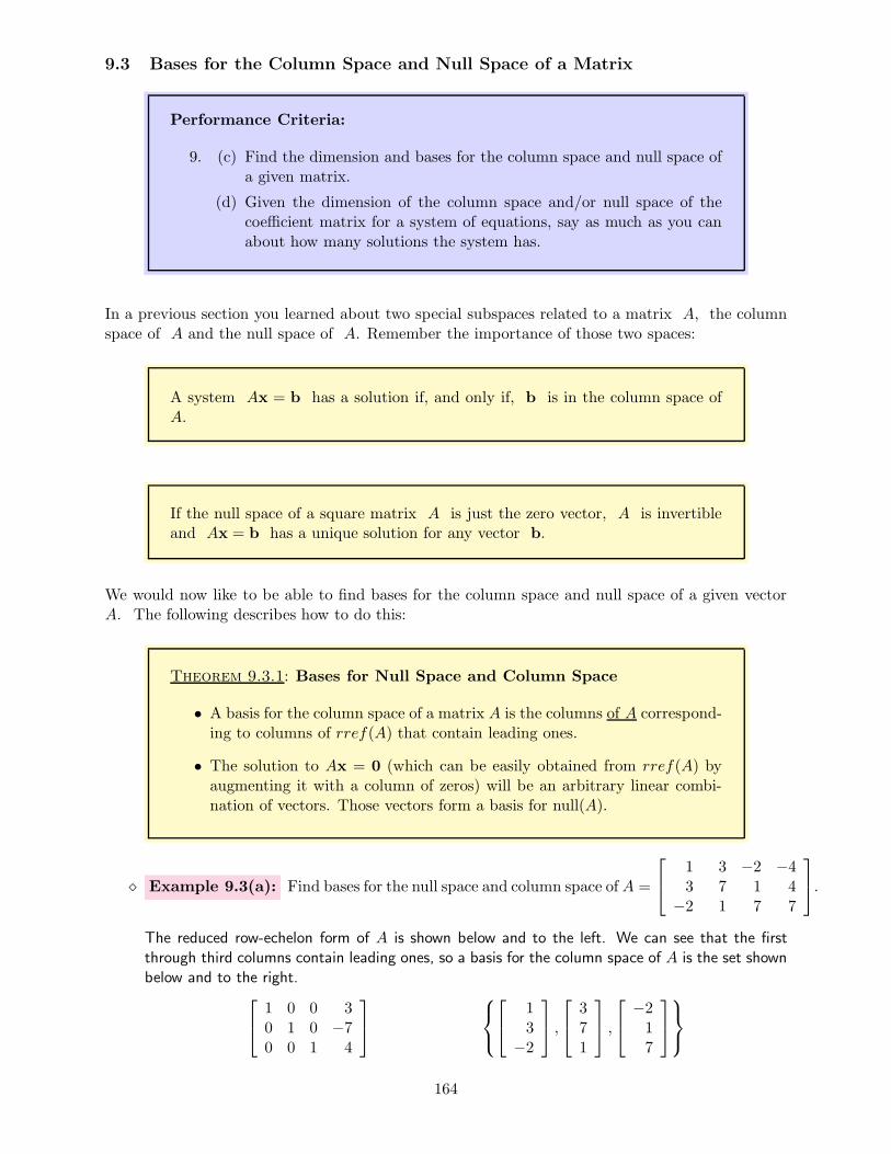
9.3 Bases for the Column Space and Null Space of a Matrix
Performance Criteria:
9. (c) Find the dimension and bases for the column space and null space ofa given matrix.
(d) Given the dimension of the column space and/or null space of thecoefficient matrix for a system of equations, say as much as you canabout how many solutions the system has.
In a previous section you learned about two special subspaces related to a matrix A, the columnspace of A and the null space of A. Remember the importance of those two spaces:
A system Ax = b has a solution if, and only if, b is in the column space ofA.
If the null space of a square matrix A is just the zero vector, A is invertibleand Ax = b has a unique solution for any vector b.
We would now like to be able to find bases for the column space and null space of a given vectorA. The following describes how to do this:
Theorem 9.3.1: Bases for Null Space and Column Space
• A basis for the column space of a matrix A is the columns of A correspond-ing to columns of rref(A) that contain leading ones.
• The solution to Ax = 0 (which can be easily obtained from rref(A) byaugmenting it with a column of zeros) will be an arbitrary linear combi-nation of vectors. Those vectors form a basis for null(A).
⋄ Example 9.3(a): Find bases for the null space and column space of A =
1 3 −2 −43 7 1 4−2 1 7 7
.
The reduced row-echelon form of A is shown below and to the left. We can see that the firstthrough third columns contain leading ones, so a basis for the column space of A is the set shownbelow and to the right.
1 0 0 30 1 0 −70 0 1 4
13−2
,
371
,
−217
164
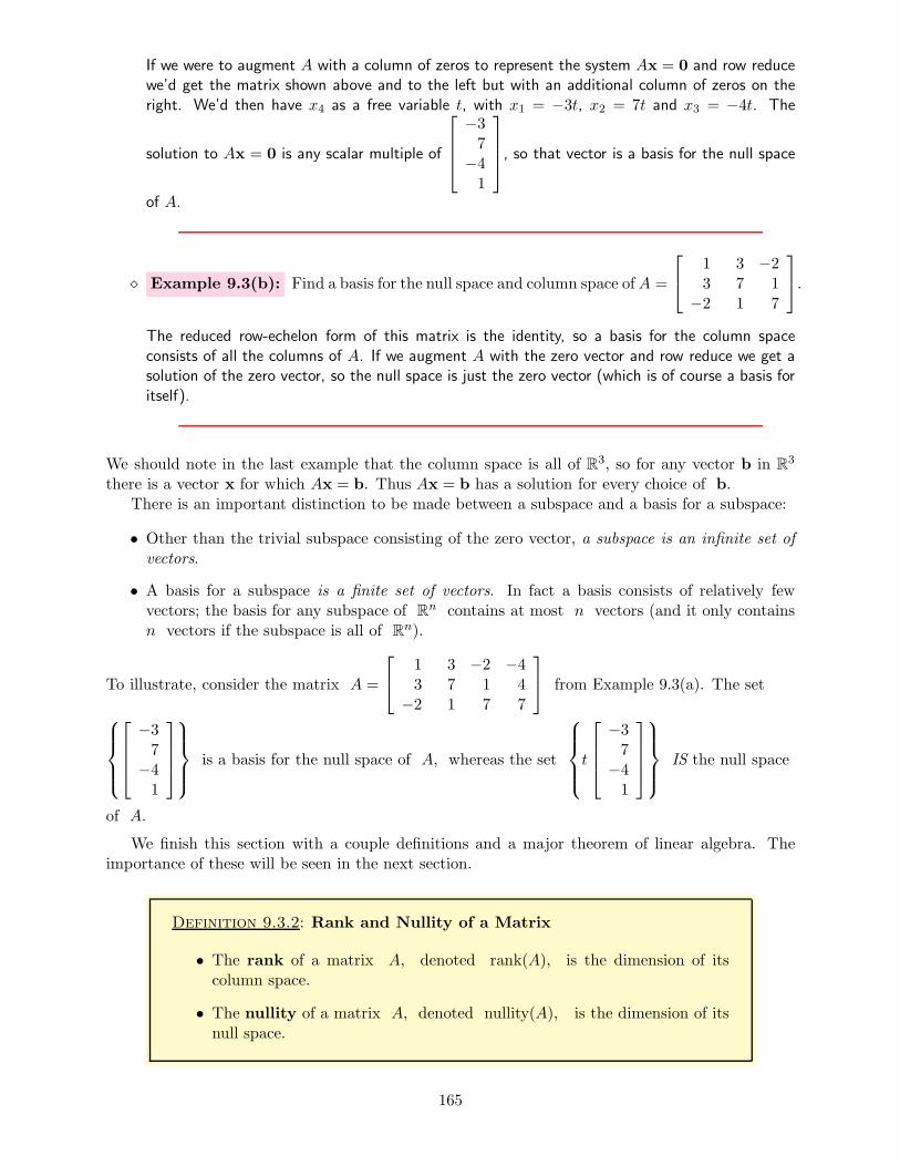
If we were to augment A with a column of zeros to represent the system Ax = 0 and row reducewe’d get the matrix shown above and to the left but with an additional column of zeros on theright. We’d then have x4 as a free variable t, with x1 = −3t, x2 = 7t and x3 = −4t. The
solution to Ax = 0 is any scalar multiple of
−37−41
, so that vector is a basis for the null space
of A.
⋄ Example 9.3(b): Find a basis for the null space and column space ofA =
1 3 −23 7 1−2 1 7
.
The reduced row-echelon form of this matrix is the identity, so a basis for the column spaceconsists of all the columns of A. If we augment A with the zero vector and row reduce we get asolution of the zero vector, so the null space is just the zero vector (which is of course a basis foritself).
We should note in the last example that the column space is all of R3, so for any vector b in R3
there is a vector x for which Ax = b. Thus Ax = b has a solution for every choice of b.There is an important distinction to be made between a subspace and a basis for a subspace:
• Other than the trivial subspace consisting of the zero vector, a subspace is an infinite set ofvectors.
• A basis for a subspace is a finite set of vectors. In fact a basis consists of relatively fewvectors; the basis for any subspace of R
n contains at most n vectors (and it only containsn vectors if the subspace is all of R
n).
To illustrate, consider the matrix A =
1 3 −2 −43 7 1 4−2 1 7 7
from Example 9.3(a). The set
−37−41
is a basis for the null space of A, whereas the set
t
−37−41
IS the null space
of A.
We finish this section with a couple definitions and a major theorem of linear algebra. Theimportance of these will be seen in the next section.
Definition 9.3.2: Rank and Nullity of a Matrix
• The rank of a matrix A, denoted rank(A), is the dimension of itscolumn space.
• The nullity of a matrix A, denoted nullity(A), is the dimension of itsnull space.
165

Theorem 9.3.3: The Rank Theorem
For an m× n matrix A, rank(A) + nullity(A) = n.
Section 9.3 Exercises
1. Consider the matrix A =
1 1 −2−3 −3 62 2 −4
, which has row-reduced form
1 1 −20 0 00 0 0
. In
this exercise you will see how to find a basis for the null space of A. All this means is thatyou are looking for a “minimal” set of vectors whose span (all possible linear combinations ofthem) give all the vectors x for which Ax = 0.
(a) Give the augmented matrix for the system of equations Ax = 0, then give its row reducedform.
(b) There are two free variables, x3 and x2. Let x3 = t and x2 = s, then find x1 (in termsof s and t). Give the vector x, in terms of s and t.
(c) Write x as the sum of two vectors, one containing only the parameter s and the othercontaining only the parameter t. Then factor s out of the first vector and t out of thesecond vector. You now have x as all linear combinations of two vectors.
(d) Those two vectors are linearly independent, since neither of them is a scalar multiple ofthe other, so both are essential in the linear combination you found in (c). They thenform a basis for the null space of A. Write this out as a full sentence, “A basis for ...”.A basis is technically a set of vectors, so use the set brackets appropriately.
2. Consider the matrix A =
1 −1 5
3 1 11
2 5 3
(a) Solve the system Ax = 0. You should get infinitely many solutions containing oneor more parameters. Give the general solution, in terms of the parameters. Give allvalues in exact form.
(b) If you didn’t already, you should be able to give the general solution as a linear combi-nation of vectors, with the scalars multiplying them being the parameter(s). Do this.
(c) The vector or vectors you see in (c) is (are) a basis for the null space of A. Give thebasis.
3. When doing part (a) of the previous exercise you should have obtained the row reduced formof the matrix A (of course you augmented it). A basis for the column space of A is thecolumns of A (NOT the columns of the row reduced form of A!) corresponding to the leadingvariables in the row reduced form of A. Give the basis for the column space of A.
166
4. Let
A =
1 1 0
2 3 −2−1 −4 6
, u1 =
29
−17
, u2 =
3152
, v1 =
8−8−4
, v2 =
50−7
.
(a) Determine whether each of u1 and u2 is in the column space of A.
(b) Find a basis for col(A). Give your answer with a brief sentence, and indicatethat the basis is a set of vectors.
(c) One of the vectors u1 and u2 IS in the column space of A. Give a linear combinationof the basis vectors that equals that vector.
5. Again let
A =
1 1 0
2 3 −2−1 −4 6
, u1 =
29
−17
, u2 =
3152
, v1 =
8−8−4
, v2 =
50−7
.
(a) Determine whether each of the vectors v1 and v2 is in null(A). Give your answer asa brief sentence.
(b) Determine a basis for null(A), giving your answer in a brief sentence.
(c) Give the linear combinations of the basis vectors of the null space for either of the vectorsv1 and v2 that are in the null space.
6. Give a sentence telling the dimensions of the column space and null space of the matrixA from the previous two exercises.
167

9.4 Solutions to Systems of Equations
Performance Criterion:
9. (e) Determine, from given information about the coefficient matrixA and vector b of a system Ax = b, whether the system hasany solutions and, if it does, whether there is more than one solution.
You may have found the last section to be a bit overwhelming, and you are probably wonderingwhy we bother with all of the definitions in that section. The reason is that those ideas form toolsand language for discussing whether a system of equations
(a) has a solution (meaning at least one) and
(b) if it does have a solution, is there only one.
Item (a) above is what mathematicians often refer to as the existence question, and item (b) is theuniqueness question. Concerns with “existence and uniqueness” of solutions is not restricted tolinear algebra; it is a big deal in the study of differential equations as well.
Consider a system of equations Ax = b. We saw previously that the product Ax is thelinear combination of the columns of A with the components of x as the scalars of the linearcombination. This means that the system will only have a solution if b is a linear combinationof the columns of A. But all of the linear combinations of the columns of A is just the span ofthose columns - the column space! the conclusion of this is as follows:
A system of equations Ax = b has a solution (meaning at least one solution)if, and only if, b is in the column space of A.
Let’s look at some consequences of this.
⋄ Example 9.4(a): Let Ax = b represent a system of five equations in five unknowns, and
suppose that rank(A) = 3. Does the system have (for certain) a solution?
Since the system has five equations in five unknowns, b is in R5. Because rank(A) = 3,
the column space of A only has dimension three, so it is not all of R5 (which of course has
dimension five). Therefore b may or may not be in the column space of A, and we can’t sayfor certain that the system has a solution.
⋄ Example 9.4(b): Let Ax = b represent a system of three equations in five unknowns,
and suppose that rank(A) = 3. Does the system have (for certain) a solution?
Because there are three equations and five unknowns, A is 5× 3 and the columns of A arein R
3. Because rank(A) = 3, the column space must then be all of R3. Therefore b will
be in the column space of A and the system has at least one solution.
168

Now suppose that we have a system Ax = b and a vector x that IS a solution to the system.Suppose also that nullity(A) 6= 0. Then there is some y 6= 0 such that Ay = 0 and
A(x+ y) = Ax+Ay = b+ 0 = b.
This shows that both x and x + y are solutions to the system, so the system does not have aunique solution. The thing that allows this to happen is the fact that the null space of A containsmore than just the zero vector. This illustrates the following:
A system of equations Ax = b can have a unique solution only if the nullity ofA is zero (that is, the null space contains only the zero vector).
Note that this says nothing about whether a system has a solution to begin with; it simply saysthat if there is a solution and the nullity is zero, then that solution is unique.
⋄ Example 9.4(c): Consider again a system Ax = b of three equations in five unknowns,
with rank(A) = 3, as in Example 9.4(b). We saw in that example that the system has atleast one solution - is there a unique solution?
We note first of all that A is 3 × 3, so the n of the Rank Theorem is three. We know thatrank(A) is three so, by the Rank Theorem, the nullity is then two. Thus the null space containsmore than just the zero vector, so the system does not have a unique solution.
⋄ Example 9.4(d): Suppose we have a system Ax = 0, with nullity(A) = 2. Does thesystem have a solution and, if it does, is it unique?
Because the system is homogeneous, it has at least one solution, the zero vector. But the nullspace contains more than just the zero vector, so the system has more than one solution, so thereis not a unique solution.
Section 9.4 Exercises
1. Suppose that the column space of a 3× 3 matrix A has dimension two. What does this tellus about the nature of the solutions to a system Ax = b?
169

9.5 Chapter 9 Exercises
1. Suppose that the column space of a 3×3 matrix A has dimension two. What does this tell us
about the nature of the solutions to a system Ax = b? Show that the vectors u1 =
[
3−1
]
,
u2 =
[
11
]
and u3 =
[
1−1
]
are linearly dependent. Then give u2 as a linear combination
of u1 and u3.
2. (a) Give three non-zero linearly dependent vectors in R3 for which removing any one of the
three leaves a linearly independent set.
(b) Give three non-zero linearly dependent vectors in R3 for which removing one vector
leaves a linearly independent set but removing a different one (of the original three)leaves a linearly dependent set.
3. Let Ax = b be a system of equations, with A an m × n matrix where m = n unlessspecified otherwise. For each situation below, determine whether the system COULD have
(i) no solution (ii) exactly one solution (iii) infinitely many solutions
Give all possibilities for each.
(a) det(A) = 0 (b) det(A) 6= 0 (c) b = 0
(d) b = 0, A invertible (e) m < n (f) m > n
(g) columns of A linearly independent (h) columns of A linearly dependent
(i) b = 0, columns of A linearly independent
(j) b = 0, columns of A linearly dependent
4. Consider the vectors u =
8−24
, v =
701
and w =
−164−8
.
(a) Is the set of all vectors x = u+ tv, where t ranges over all real numbers, a subspace ofR3? If so, give a basis for the subspace; if not, tell why not.
(b) Is the set of all vectors x = u+ tw, where t ranges over all real numbers, a subspace ofR3? If so, give a basis for the subspace; if not, tell why not.
(c) Is the set of all vectors x = u+sv+ tw, where t ranges over all real numbers, a subspaceof R3? If so, give a basis for the subspace; if not, tell why not.
5. Consider the matrix A =
2 2 2
−2 5 2
8 1 4
.
170

(a) Find a basis for row(A), the row space of A. What is the dimension of row(A)? (Youcan finddirections for finding row(A) in your book or in the definitions and theoremshandouts.)
(b) Find a basis for col(A), the column space of A. What is the dimension of col(A)?
6. Give bases for the null and column spaces of the matrix A =
−6 3 302 −1 −10−4 2 20
.
7. Consider the system of equations
x1 − 2x2 + 3x3 = 4
2x1 + x2 − 4x3 = 3
−3x1 + 4x2 − x3 = −2.
(a) Determine how many solutions the system has.
(b) Give the form Ax = b for the system.
(c) Find a basis for the column space of A.
(d) Find a basis for the null space of A.
8. Now consider the system of equations
x1 + 2x3 = −5−2x1 + 5x2 = 11
2x1 + 5x2 + 8x3 = −7.
(a) Determine how many solutions the system has.
(b) Give the form Ax = b for the system.
(c) Find a basis for the column space of A.
(d) Find a basis for the null space of A.
9. The system
x1 + 2x3 = −1−2x1 + 5x2 = −12x1 + 5x2 + 8x3 = −5
DOES have a solution. (Infinitely many, actually.)
How does the Ax = b form of this system compare to that of the previous one? How arethey similar and how are they different?
10. (a) Give a 3 × 3 matrix B for which the column space has dimension one. (Hint: Whatkind of subspace of R
3 has dimension one?)
(b) Find a basis for the column space of B.
(c) What should the dimension of the null space of B be?
(d) Find a basis for the null space of B.
171

172
10 Linear Transformations
Outcome:
10. Understand linear transformations, their compositions, and their applica-tion to homogeneous coordinates. Understand representations of vectorswith respect to different bases.
Performance Criteria:
(a) Evaluate a transformation.
(b) Determine the formula for a transformation in R2 or R
3 that hasbeen described geometrically.
(c) Determine whether a given transformation from Rm to R
n is linear. Ifit isn’t, give a counterexample; if it is, demonstrate this algebraicallyand/or give the standard matrix representation of the transformation.
(d) Draw an arrow diagram illustrating a transformation that is linear,or that is not linear.
(e) For a transformation T : R2 → R2, show the graphical differences
between (a) T (cu) and cTu, and (b) T (u+ v) and Tu+ Tv.
(f) Find the composition of two transformations.
(g) Find matrices that perform combinations of dilations, reflections, ro-tations and translations in homogenous coordinates.
173

10.1 Transformations of Vectors
Performance Criteria:
10. (a) Evaluate a transformation.
(b) Determine the formula for a transformation in R2 or R
3 that hasbeen described geometrically.
Back in a “regular” algebra class you might have considered a function like f(x) =√x+ 5,
and you may have discussed the fact that this function is only valid for certain values of x. Whenconsidering functions more carefully, we usually “declare” the function before defining it:
Let f : [−5,∞)→ R be defined by f(x) =√x+ 5
Here the set [−5,∞) of allowable “inputs” is called the domain of the function, and the set R issometimes called the codomain or target set. Those of you with programming experience willrecognize the process of first declaring the function, then defining it. Later you might “call” thefunction, which in math we refer to as “evaluating” it.
In a similar manner we can define functions from one vector space to another, like
Define T : R2 → R3 by T
([
x1x2
])
=
x1 + x2x2
x21
We will call such a function a transformation, hence the use of the letter T . (When we havea second transformation, we’ll usually call it S.) The word “transformation” implies that onevector is transformed into another vector. It should be clear how a transformation works:
⋄ Example 10.1(a): Find T
([
−35
])
for the transformation defined above.
T
([
−35
])
=
−3 + 55
(−3)2
=
259
It gets a bit tiresome to write both parentheses and brackets, so from now on we will dispense withthe parentheses and just write
T
[
−35
]
=
259
At this point we should note that you have encountered other kinds of transformations. Forexample, taking the derivative of a function results in another function,
d
dx(x3 − 5x2 + 2x− 1) = 3x2 − 10x+ 2,
so the action of taking a derivative can be thought of as a transformation. Such transformationsare often called operators.
Sometimes we will wish to determine the formula for a transformation from R2 to R
2 orR3 to R
3 that has been described geometrically.
174

⋄ Example 10.1(b): Determine the formula for the transformation T : R2 → R2 that
reflects vectors across the x-axis.
First we might wish to draw a picture to see what such a transformationdoes to a vector. To the right we see the vectors u = [3, 2] and v =[−1,−3], and their transformations Tu = [3,−2] and Tv = [−1, 3].From these we see that what the transformation does is change the signof the second component of a vector. Therefore
T
[
x1x2
]
=
[
x1−x2
]
4
4
-4
-4
u
Tuv
Tv
⋄ Example 10.1(c): Determine the formula for the transformation T : R3 → R3 that
projects vectors onto the xy-plane.
It is a little more difficult to draw a picture for this one, but to the rightyou can see an attempt to illustrate the action of this transformation ona vector u. Note that in projecting a vector onto the xy-plane, thex- and y-coordinates stay the same, but the z-coordinate becomes zero.The formula for the transformation is then
T
x
y
z
=
x
y
0
u
Tux
y
z
We conclude this section with a very important observation. Consider the matrix
A =
5 10 −3−1 2
and define TAx = Ax for every vector for which Ax is defined. This transformation acts onvectors in R
2 and “returns” vectors in R3. That is, TA : R2 → R
3. In general, we can use anym× n matrix A to define a transformation TA : Rn → R
m in this manner. In the next sectionwe will see that such transformations have a desirable characteristic, and that every transformationwith that characteristic can be represented by multiplication by a matrix.
175

10.2 Linear Transformations
Performance Criteria:
10. (c) Determine whether a given transformation from Rm to R
n is linear. Ifit isn’t, give a counterexample; if it is, demonstrate this algebraicallyand/or give the standard matrix representation of the transformation.
(d) Draw an arrow diagram illustrating a transformation that is linear,or that is not linear.
(e) For a transformation T : R2 → R2, show the graphical differences
between (a) T (cu) and cTu, and (b) T (u+ v) and Tu+ Tv.
To begin this section, recall the transformation from Example 10.1(b) that reflects vectors inR2 across the x-axis. In the drawing below and to the left we see two vectors u and v that are
added, and then the vector u+ v is reflected across the x-axis. In the drawing below and to theright the same vectors u and v are reflected across the x-axis first, then the resulting vectorsTu and Tv are added.
uv
u+ v
T (u+ v)
y
x
uv
Tu
Tv
Tu+ Tv)
y
x
Note that T (u + v) = Tu + Tv. Not all transformations have this property, but those that dohave it, along with an additional property, are very important:
Definition 10.2.1: Linear Transformation
A transformation T : Rm → Rn is called a linear transformation if, for every
scalar c and every pair of vectors u and v in Rm
1) T (u+ v) = T (u) + T (v) and
2) T (cu) = cT (u).
Note that the above statement describes how a transformation T interacts with the twooperations of vectors, addition and scalar multiplication. It tells us that if we take two vectors inthe domain and add them in the domain, then transform the result, we will get the same thing as ifwe transform the vectors individually first, then add the results in the codomain. We will also getthe same thing if we multiply a vector by a scalar and then transform as we will if we transformfirst, then multiply by the scalar.This is illustrated in the mapping diagram at the top of the nextpage.
176

T
Rm
Rn
w
cw
u
v
u+ v
T (cw) = cTw
Tw
Tu
Tv
T (u+ v) = Tu+ Tv
The following two mapping diagrams are for transformations R and S that ARE NOT linear:
TRm
Rn
w
cw T (cw)
Tw
cTw
TRm
Rn
u
v
u+ v
Tu
Tv
T (u+ v) Tu+ Tv
⋄ Example 10.2(a): Let A be an m×n matrix. Is TA : Rn → Rm defined by TAx = Ax a
linear transformation?
We know from properties of multiplying a vector by a matrix that
TA(u+ v) = A(u+ v) = Au+Av = TAu+ TAv, TA(cu) = A(cu) = cAu = cTAu.
Therefore TA is a linear transformation.
⋄ Example 10.2(b): Is T : R2 → R
3 defined by T
[
x1x2
]
=
x1 + x2x2
x21
a linear
transformation? If so, show that it is; if not, give a counterexample demonstrating that.
177

A good way to begin such an exercise is to try the two properties of a linear transformation forsome specific vectors and scalars. If either condition is not met, then we have our counterexample,and if both hold we need to show they hold in general. Usually it is a bit simpler to check thecondition T (cu) = cTu. In our case, if c = 2 and vecu = [2, 3, 4],
T
(
2
[
34
])
= T
[
68
]
=
14836
and 2T
[
34
]
= 2
749
=
14818
Because T (cu) 6= cTu for our choices of c and u, T is not a linear transformation.
The next example shows the process required to show in general that a transformation is linear.
⋄ Example 10.2(c): Determine whether T : R3 → R2 defined by T
x1x2x3
=
[
x1 + x2x2 − x3
]
is linear. If it is, prove it in general; if it isn’t, give a specific counterexample.
First let’s try a specific scalar c = 2 and two specific vectors u =
123
and v =
4−56
. (I
threw the negative in there just in case something funny happens when everything is positive.)Then
T
123
+
4−56
= T
5−39
=
[
2−12
]
and
T
123
+ T
4−56
=
[
3−1
]
+
[
−1−11
]
=
[
2−12
]
so the first condition of linearity appears to hold. Let’s prove it in general. Let u =
u1u2u3
and
v =
v1v2v3
be arbitrary (that is, randomly selected) vectors in R3. Then
T (u+ v) = T
u1u2u3
+
v1v2v3
= T
u1 + v1u2 + v2u3 + v3
=
[
u1 + v1 + u2 + v2(u2 + v2)− (u3 + v3)
]
=
[
u1 + u2 + v1 + v2(u2 − u3) + (v2 − v3)
]
=
[
u1 + u2u2 − u3
]
+
[
v1 + v2v2 − v3
]
= T
u1u2u3
+T
v1v2v3
= T (u)+T (v)
178

This shows that the first condition of linearity holds in general. Let u again be arbitrary, alongwith the scalar c. Then
T (cu) = T
c
u1u2u3
= T
cu1cu2cu3
=
[
cu1 + cu2cu2 − cu3
]
=
[
c(u1 + u2)c(u2 − u3)
]
= c
[
u1 + u2u2 − u3
]
= cT
u1u2u3
= cT (u)
so the second condition holds as well, and T is a linear transformation.
There is a handy fact associated with linear transformations:
Theorem 10.2.2: If T is a linear transformation, then T (0) = 0.
Note that this does not say that if T (0) = 0, then T is a linear transformation, as you will seebelow. However, the contrapositive of the above statement tells us that if T (0) 6= 0, then T is nota linear transformation.
When working with coordinate systems, one operation we often need to carry out is a trans-lation, which means a shift of all points the same distance and direction. The transformation inthe following example is a translation in R
2.
⋄ Example 10.2(d): Let a and b be any real numbers, with not both of them zero. Define
T : R2 → R2 by T
[
x1x2
]
=
[
x1 + a
x2 + b
]
. Is T a linear transformation?
Since T
[
00
]
=
[
a
b
]
6=[
00
]
(since not both a and b are zero), T is not a linear transformation.
⋄ Example 10.2(e): Determine whether T : R2 → R2 defined by T
[
x1x2
]
=
[
x1 + x2x1x2
]
is
linear. If it is, prove it in general; if it isn’t, give a specific counterexample.
It is easy to see that T (0) = 0, so we can’t immediately rule out T being linear, as we didin the last example. Let’s do a quick check of the first condition of the definition of a linear
transformation with an example. Let u =
[
−32
]
and v =
[
14
]
. Then
T (u+ v) = T
([
−32
]
+
[
14
])
= T
[
−26
]
=
[
4−12
]
and
Tu+ Tv = T
[
−32
]
+ T
[
14
]
=
[
−1−6
]
+
[
54
]
=
[
4−2
]
Clearly T (u+ v) 6= Tu+ Tv, so T is not a linear transformation.
179
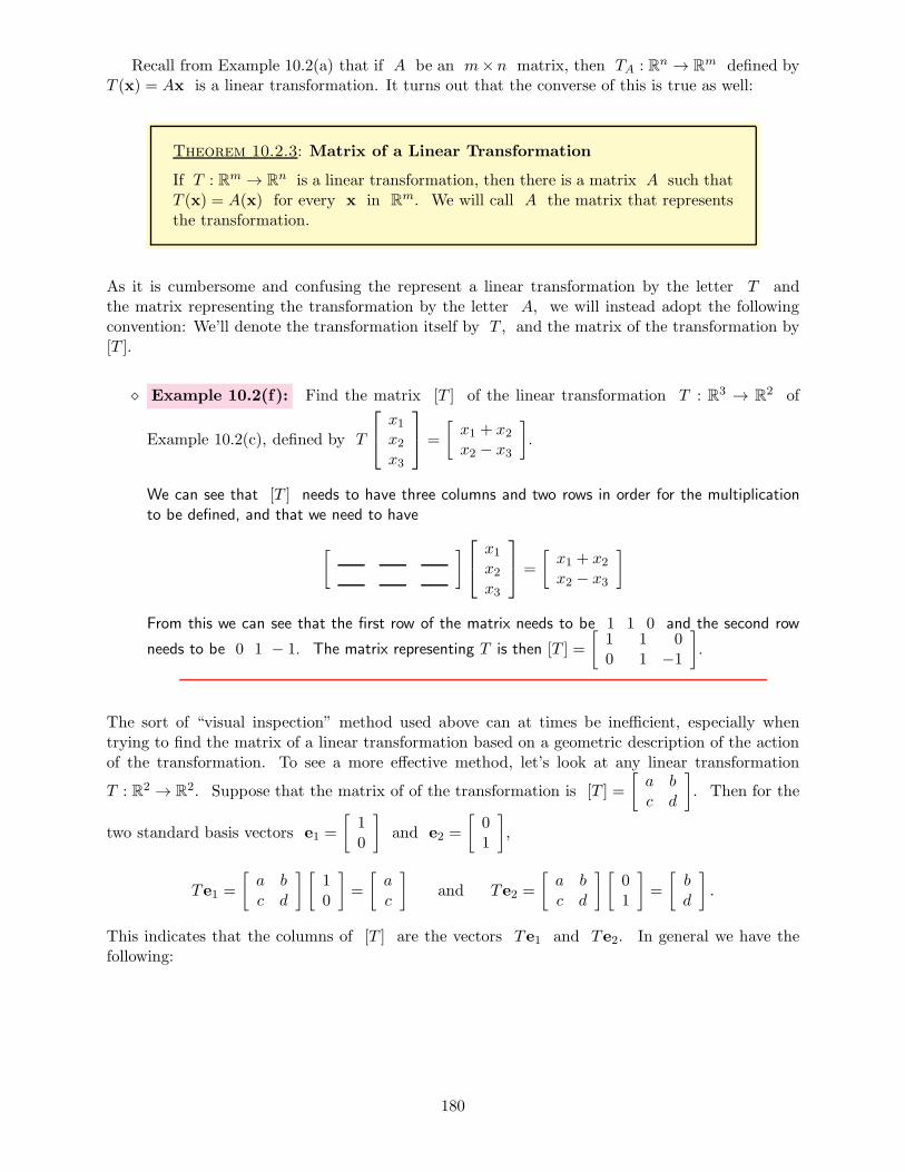
Recall from Example 10.2(a) that if A be an m×n matrix, then TA : Rn → Rm defined by
T (x) = Ax is a linear transformation. It turns out that the converse of this is true as well:
Theorem 10.2.3: Matrix of a Linear Transformation
If T : Rm → Rn is a linear transformation, then there is a matrix A such that
T (x) = A(x) for every x in Rm. We will call A the matrix that represents
the transformation.
As it is cumbersome and confusing the represent a linear transformation by the letter T andthe matrix representing the transformation by the letter A, we will instead adopt the followingconvention: We’ll denote the transformation itself by T , and the matrix of the transformation by[T ].
⋄ Example 10.2(f): Find the matrix [T ] of the linear transformation T : R3 → R2 of
Example 10.2(c), defined by T
x1x2x3
=
[
x1 + x2x2 − x3
]
.
We can see that [T ] needs to have three columns and two rows in order for the multiplicationto be defined, and that we need to have
[ ]
x1x2x3
=
[
x1 + x2x2 − x3
]
From this we can see that the first row of the matrix needs to be 1 1 0 and the second row
needs to be 0 1 − 1. The matrix representing T is then [T ] =
[
1 1 00 1 −1
]
.
The sort of “visual inspection” method used above can at times be inefficient, especially whentrying to find the matrix of a linear transformation based on a geometric description of the actionof the transformation. To see a more effective method, let’s look at any linear transformation
T : R2 → R2. Suppose that the matrix of of the transformation is [T ] =
[
a b
c d
]
. Then for the
two standard basis vectors e1 =
[
10
]
and e2 =
[
01
]
,
Te1 =
[
a b
c d
] [
10
]
=
[
a
c
]
and Te2 =
[
a b
c d
] [
01
]
=
[
b
d
]
.
This indicates that the columns of [T ] are the vectors Te1 and Te2. In general we have thefollowing:
180
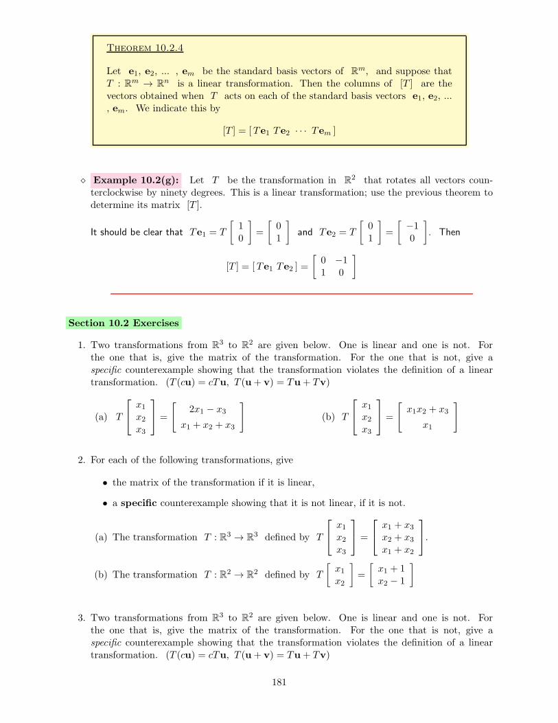
Theorem 10.2.4
Let e1, e2, ... , em be the standard basis vectors of Rm, and suppose that
T : Rm → Rn is a linear transformation. Then the columns of [T ] are the
vectors obtained when T acts on each of the standard basis vectors e1, e2, ..., em. We indicate this by
[T ] = [Te1 Te2 · · · Tem ]
⋄ Example 10.2(g): Let T be the transformation in R2 that rotates all vectors coun-
terclockwise by ninety degrees. This is a linear transformation; use the previous theorem todetermine its matrix [T ].
It should be clear that Te1 = T
[
10
]
=
[
01
]
and Te2 = T
[
01
]
=
[
−10
]
. Then
[T ] = [Te1 Te2 ] =
[
0 −11 0
]
Section 10.2 Exercises
1. Two transformations from R3 to R
2 are given below. One is linear and one is not. Forthe one that is, give the matrix of the transformation. For the one that is not, give aspecific counterexample showing that the transformation violates the definition of a lineartransformation. (T (cu) = cTu, T (u+ v) = Tu+ Tv)
(a) T
x1x2x3
=
[
2x1 − x3
x1 + x2 + x3
]
(b) T
x1x2x3
=
[
x1x2 + x3
x1
]
2. For each of the following transformations, give
• the matrix of the transformation if it is linear,
• a specific counterexample showing that it is not linear, if it is not.
(a) The transformation T : R3 → R3 defined by T
x1x2x3
=
x1 + x3x2 + x3x1 + x2
.
(b) The transformation T : R2 → R2 defined by T
[
x1x2
]
=
[
x1 + 1x2 − 1
]
3. Two transformations from R3 to R
2 are given below. One is linear and one is not. Forthe one that is, give the matrix of the transformation. For the one that is not, give aspecific counterexample showing that the transformation violates the definition of a lineartransformation. (T (cu) = cTu, T (u+ v) = Tu+ Tv)
181

(a) T
x1x2x3
=
[
2x1 − x3
x1 + x2 + x3
]
(b) T
x1x2x3
=
[
x1x2 + x3
x1
]
4. For each of the following transformations, give
• the matrix of the transformation if it is linear,
• a specific counterexample showing that it is not linear, if it is not.
(a) The transformation T : R3 → R3 defined by T
x1x2x3
=
x1 + x3x2 + x3x1 + x2
.
(b) The transformation T : R2 → R2 defined by T
[
x1x2
]
=
[
x1 + 1x2 − 1
]
5. (a) The transformation T : R2 → R3 defined by T
[
x1x2
]
=
x1 + 2x23x2 − 5x1
x1
is linear.
Show that, for vectors u =
[
u1u2
]
and v =
[
v1v2
]
, T (u+ v) = Tu+ Tv. Do this
via a string of equal expressions, beginning with T (u+ v) and ending with Tu+ Tv.
(b) Give the matrix for the transformation from part (a).
6. For each of the following, a transformation T : R2 → R2 is given by describing its action on
a vector x = [x1, x2]. For each transformation, determine whether it is linear by
• finding T (cu) and c(Tu) and seeing if they are equal,
• finding T (u+ v) and T (u) + T (v) and seeing if they are equal.
For any that you find to be linear, say so. For any that are not, say so and produce a specificcounterexample to one of the two conditions for linearity.
(a) T
[
x1
x2
]
=
[
x2
x1 + x2
]
(b) T
[
x1
x2
]
=
[
x1 + x2
x1 x2
]
(c) T
[
x1
x2
]
=
[ |x1||x2|
]
(d) T
[
x1
x2
]
=
[
3x1x1 − x2
]
7. For each of the transformations from the previous exercise that are linear, give the standardmatrix of the transformation.
182

10.3 Compositions of Transformations
Performance Criterion:
10. (f) Find the composition of two transformations.
It is likely that at some point in your past you have seen the concept of the composition of twofunctions; if the functions were denoted by f and g, one composition of them is the new functionf g. We call this new function “f of g”, and we must describe how it works. This is simple -for any x, (f g)(x) = f [g(x)]. That is, g acts on x, and f then acts on the result. There isanother composition, g f , which is defined the same way (but, of course, in the opposite order).For specific functions, you were probably asked to find the new rule for these two compositions.Here’s a reminder of how that is done:
⋄ Example 10.3(a): For the functions f(x) = 2x− 1 and g(x) = 4x− x2, find the formulasfor the composition functions f g and g f .
Basic algebra gives us
(f g)(x) = f [g(x)] = f [4x− x2] = 2(4x − x2)− 1 = 8x− 2x2 − 1 = −2x2 + 8x− 1
and
(g f)(x) = g[f(x)] = g[2x− 1] = 4(2x− 1)− (2x− 1)2 =
(8x− 4)− (4x2 − 4x+ 1) = 8x− 4− 4x2 + 4x− 1 = −4x2 + 12x − 5
The formulas are then (f g)(x) = −2x2 + 8x− 1 and (g f)(x) = −4x2 + 12x− 5.
Worthy of note here is that the two compositions f g and g f are not the same!One thing that was probably glossed over when you first saw this concept was the fact that
the range (all possible outputs) of the first function to act must fall within the domain (allowableinputs) of the second function to act. Suppose, for example, that f(x) =
√x− 4 and g(x) = x2.
The function f will be undefined unless x is at least four; we indicate this by writing f : [4,∞)→ R.This means that we need to restrict g in such a way as to make sure that g(x) ≥ 4 if we wish toform the composition f g. One simple way to do this is to restrict the domain of g to [2,∞). (Wecould include the interval (−∞,−2] also, but for the sake of simplicity we will just use the positiveinterval.) The range of g is then [4,∞), which coincides with the domain of f . We now see howthese ideas apply to transformations, and we see how to carry out a process like that of Example10.3(a) for transformations.
⋄ Example 10.3(b): Let S : R3 → R2 and T : R2 → R
2 be defined by
S
x1x2x3
=
[
x21x2x3
]
, T
[
x1x2
]
=
[
x1 + 3x22x2 − x1
]
Determine whether each of the compositions S T and T S exists, and find a formula foreither of them that do.
183

Since the domain of S is R3 and the range of T is a subset of R2, the composition S T doesnot exist. The range of S falls within the domain of T , so the composition T S does exist. Itsequation is found by
(T S)(x) = T
S
x1x2x3
= T
[
x21x2x3
]
=
[
x21 + 3x2x32x2x3 − x21
]
Let’s formally define what we mean by a composition of two transformations.
Definition 10.3.1 Composition of Transformations
Let S : Rp → Rn and T : Rm → R
p be transformations. The composition ofS and T , denoted by S T , is the transformation S T : Rm → R
n definedby
(S T )x = S(Tx)
for all vectors x in Rm.
Although the above definition is valid for compositions of any transformations between vectorspaces, we are primarily interested in linear transformations. Recall that any linear transformationbetween vector spaces can be represented by matrix multiplication for some matrix. Suppose thatS : R3 → R
3 and T : R2 → R3 are linear transformations that can be represented by the matrices
[S] =
3 −1 50 2 14 0 −3
and [T ] =
2 7−6 11 −4
respectively.
⋄ Example 10.3(c): For the transformations S and T just defined, find (S T ) x =
(S T )[
x1x2
]
. Then find the matrix of the transformation S T .
We see that
(S T )x = S(Tx) = S
2 7−6 11 −4
[
x1x2
]
= S
2x1 + 7x2−6x1 + x2x1 − 4x2
=
3 −1 50 2 14 0 −3
2x1 + 7x2−6x1 + x2x1 − 4x2
184

=
3(2x1 + 7x2)− (−6x1 + x2) + 5(x1 − 4x2)0(2x1 + 7x2) + 2(−6x1 + x2) + (x1 − 4x2)4(2x1 + 7x2) + 0(−6x1 + x2)− 3(x1 − 4x2)
=
17x1 + 0x2−11x1 − 2x25x1 + 40x2
From this we can see that the matrix of S T is [S T ] =
17 0−11 −2
5 40
.
Recall that the linear transformations of this example have matrices [S] and [T ], and we findthat
[S][T ] =
3 −1 50 2 14 0 −3
2 7−6 11 −4
=
17 0−11 −2
5 40
.
This illustrates the following:
Theorem 10.3.2 Matrix of a Composition
Let S : Rp → Rn and T : Rm → R
p be linear transformations with matrices[S] and [T ]. Then
[S T ] = [S][T ]
Section 10.3 Exercises
1. Consider the linear transformations S
[
x
y
]
=
x+ y
2x−3y
, T
[
x
y
]
=
[
5x− y
x+ 4y
]
.
(a) Since both of these are linear transformations, there are matrices A and B representingthem. Give those two matrices (A for S, B for T ).
(b) Give equations for either (or both) of the compositions S T and T S that exist.
(c) Give the matrix for either (or both) of the compositions that exist.
(d) Find either (or both) of AB and BA that exist.
(e) What did you notice in parts (c) and (d)? Answer this with a complete sentence.
185
10.4 Chapter 10 Exercises
1. Consider the matrix A =
[
1 1 −3−1 1 1
]
, which row reduces to
[
1 0 −20 1 −1
]
.
(a) Give a basis for the null space of A.
(b) Give a basis for the column space of A.
(c) The transformation T defined by T (x) = Ax is a linear transformation. Fill in eachblank with the correct R
n:
T : →
(d) A mapping f : C → D is one-to-one if whenever x 6= y, it is also true thatf(x) 6= f(y). Give a specific example showing that the mapping T defined in (c) isNOT one-to-one. (Hint: I did not include parts (a) and (b) just to keep you off thestreets a bit longer!)
(e) A mapping f : C → D is onto if for every element y in D there is some elementx in C such that y = f(x). Tell why we know that the transformation T from (c)is onto, using one sentence and language from our class.
5. Now consider the matrix B =
1 0−3 12 1
, which row reduces to
1 00 10 0
.
(a) Give a basis for the null space of B.
(b) Give a basis for the column space of B.
(c) The transformation T defined by T (x) = Bx is a linear transformation. Fill in eachblank with the correct R
n:
T : →
(d) Explain, in a single sentence and using language from our class, why the transformationT defined in (c) is not onto.
186
11 Eigenvalues, Eigenspaces and Diagonalization
Outcome:
11. Understand eigenvalues and eigenspaces, diagonalization.
Performance Criteria:
(a) Determine whether a given vector is an eigenvector for a matrix; if itis, give the corresponding eigenvalue.
(b) Determine eigenvectors and corresponding eigenvalues for lineartransformations in R
2 or R3 that are described geometrically.
(c) Find the characteristic polynomial for a 2× 2 or 3× 3 matrix. Useit to find the eigenvalues of the matrix.
(d) Give the eigenspace Ej corresponding to an eigenvalue λj of amatrix.
(e) Diagonalize a matrix; know the forms of the matrices P and D fromP−1AP = D.
(f) Write a system of linear differential equations in matrix-vector form.Write the initial conditions in vector form.
(g) Solve a system of two linear differential equations; solve an initialvalue problem for a system of two linear differential equations.
187

11.1 An Introduction to Eigenvalues and Eigenvectors
Performance Criteria:
11. (a) Determine whether a given vector is an eigenvector for a matrix; if itis, give the corresponding eigenvalue.
(b) Determine eigenvectors and corresponding eigenvalues for lineartransformations in R
2 or R3 that are described geometrically.
Recall that the two main features of a vector in Rn are direction and magnitude. In general,
when we multiply a vector x in Rn by an n × n matrix A, the result Ax is a new
vector in Rn whose direction and magnitude are different than those of x. For every square
matrix A there are some vectors whose directions are not changed (other than perhaps havingtheir directions reversed) when multiplied by the matrix. That is, multiplying x by A givesthe same result as multiplying x by a scalar. It is very useful for certain applications to identifywhich vectors those are, and what the corresponding scalar is. Let’s use the following example toget started:
⋄ Example 11.1(a): Multiply the matrix A =
[
−4 −63 5
]
times the vectors u =[
13
]
and v =
[
2−1
]
and determine whether multiplication by A is the same as
multiplying by a scalar in either case.
Au =
[
−4 −63 5
] [
13
]
=
[
−2218
]
, Av =
[
−4 −63 5
] [
2−1
]
=
[
−21
]
For the first multiplication there appears to be nothing special going on. For the second multipli-cation, the effect of multiplying v by A is the same as simply multiplying v by −1. Notealso that
[
−4 −63 5
] [
−63
]
=
[
6−3
]
,
[
−4 −63 5
] [
8−4
]
=
[
−84
]
It appears that if we multiply any scalar multiple of v by A the same thing happens; the resultis simply the negative of the vector. That is, Ax = (−1)x for every scalar multiple of x.
We say that v =
[
2−1
]
and all of its scalar multiples are eigenvectors of A, with
corresponding eigenvalue −1. Here is the formal definition of an eigenvalue and eigenvector:
188

Definition 11.1.1: Eigenvalues and Eigenvectors
A scalar λ is called an eigenvalue of a matrix A if there is a nonzero vectorx such that
Ax = λx.
The vector x is an eigenvector corresponding to the eigenvalue λ.
One comment is in order at this point. Suppose that x has n components. Then λx doesas well, so A must have n rows. However, for the multiplication Ax to be possible, A mustalso have n columns. For this reason, only square matrices have eigenvalues and eigenvectors. Wenow see how to determine whether a vector is an eigenvector of a matrix.
⋄ Example 11.1(b): Determine whether either of the vectors w1 =
[
4−1
]
and w2 =[
−33
]
are eigenvectors for the matrix A =
[
−4 −63 5
]
of Example 11.1(a). If either is,
give the corresponding eigenvalue.
We see that
Aw1 =
[
−4 −63 5
] [
4−1
]
=
[
−107
]
and Aw2 =
[
−4 −63 5
] [
−33
]
=
[
−66
]
w1 is not an eigenvector of A because there is no scalar λ such that Aw1 is equal to λw1.w2 IS an eigenvector, with corresponding eigenvalue 2, because Aw2 = 2w2.
Note that for the 2× 2 matrix A of Examples 11.1(a) and (b) we have seen two eigenvaluesnow. It turns out that those are the only two eigenvalues, which illustrates the following:
Theorem 11.1.2: The number of eigenvalues of an n× n matrix is at most n.
Do not let the use of the Greek letter lambda intimidate you - it is simply some scalar! Itis tradition to use λ to represent eigenvalues. Now suppose that x is an eigenvector of ann×n matrix A, with corresponding eigenvalue λ, and let c be any scalar. Then for the vectorcx we have
A(cx) = c(Ax) = c(λx) = (cλ)x = λ(cx)
This shows that any scalar multiple of x is also an eigenvector of A with the same eigenvalueλ. The set of all scalar multiples of x is of course a subspace of R
n, and we call it theeigenspace corresponding to λ. x, or any scalar multiple of it, is a basis for the eigenspace.The two eigenspaces you have seen so far have dimension one, but an eigenspace can have a higherdimension.
189

Definition 11.1.3: Eigenspace Corresponding to an Eigenvalue
For a given eigenvalue λj of an n × n matrix A, the eigenspace Ej cor-responding to λ is the set of all eigenvectors corresponding to λj. It is asubspace of R
n.
So far we have been looking at eigenvectors and eigenvalues from a purely algebraic viewpoint,but looking to see if the equation Ax = λx held for some vector x and some scalar λ. It isuseful to have some geometric understanding of eigenvectors and eigenvalues as well. In the nexttwo examples we consider eigenvectors and eigenvalues of two linear transformations in R
2 froma geometric standpoint. Note that the equation Ax = λx tells us that x is an eigenvector if theaction of A on it leaves its direction unchanged or opposite of what it was.
⋄ Example 11.1(c): Consider the transformation T that reflects very vector in R2 over
the line l with equation y = 12x; this is a linear transformation. Determine the eigenvectors
and corresponding eigenvalues for this transformation.
We begin by observing that any vector that lies on l will beunchanged by the reflection, so it will be an eigenvector, witheigenvalue λ = 1. These vectors are all the scalar multiplesof x = [2, 1]; see the picture to the right. A vector not on theline, u, is shown along with its reflection Tu as well. Wecan see that its direction is changed, so it is not an eigenvector.However, for any vector v that is perpendicular to l we haveTv = −v. Therefore any such vector is an eigenvector witheigenvalue λ = −1. Those vectors are all the scalar multiplesof x = [−1, 2].
xu
Tu
v
Tv
l
x
y
⋄ Example 11.1(d): Let T be the transformation T that rotates every vector in R2 by
thirty degrees counterclockwise; this is a linear transformation. Determine the eigenvectorsand corresponding eigenvalues for this transformation.
Because every vector in R2 will be rotated by thirty degrees, the direction of every vector will
be altered, so there are no eigenvectors for this transformation.
Our conclusion in Example 11.1(d) is correct in one sense, but incorrect in another. Geometrically,in a way that we can see, the conclusion is correct. Algebraically, the transformation has eigenvec-tors, but their components are complex numbers, and the corresponding eigenvalues are complexnumbers as well. In this course we will consider only real eigenvectors and eigenvalues.
190

Section 11.1 Exercises
1. Consider the matrix A =
[
1 1
−2 4
]
.
(a) Find Ax for each of the following vectors: x1 = [3, 6], x2 = [2,−1], x3 = [1, 5],x4 = [−3,−3], x5 = [2, 2]
(b) Give the vectors from part (a) that are eigenvectors and, for each, give the correspondingeigenvalue.
(c) Give one of the eigenvalues that you have found. Then give the general form for anyeigenvector corresponding to that eigenvalue.
(d) Repeat part (c) for the other eigenvalue that you have found.
2. Now consider the matrix B =
[
5 −26 −2
]
. One eigenvalue of this matrix is λ = 2. The
objective of this exercise is to describe the associated eigenspace.
(a) Since 2 is an eigenvalue of B, for some vector x = [x1, x2] we must have Bx = 2x. Writethe system of equations represented by this equation.
(b) You should be able to rewrite your system of equations from (a) in a form that isequivalent to the vector equation Cx = 0. Do that and solve for the vector x.
(c) Describe the eigenspace of B associated with the eigenvector λ = 2.
191

11.2 Finding Eigenvalues and Eigenvectors
Performance Criteria:
11. (c) Find the characteristic polynomial for a 2× 2 or 3× 3 matrix. Useit to find the eigenvalues of the matrix.
(d) Give the eigenspace Ej corresponding to an eigenvalue λj of amatrix.
So where are we now? We know what eigenvectors, eigenvalues and eigenspaces are, and weknow how to determine whether a vector is an eigenvector of a matrix. There are two big questionsat this point:
• Why do we care about eigenvalues and eigenvectors?
• If we are just given a square matrix A, how do we find its eigenvalues and eigenvectors?
We will not see the answer to the first question for a bit, but we’ll now tackle answering thesecond question. We begin by rearranging the eigenvalue/eigenvector equation Ax = λx a bit.First, we can subtract λx from both sides to get
Ax− λx = 0.
Note that the right side of this equation must be the zero vector, because both Ax and λx arevectors. At this point we want to factor x out of the left side, but if we do so carelessly we willget a factor of A − λ, which makes no sense because A is a matrix and λ is a scalar! Note,however, that multiplying a vector by the scalar λ is the same as multiplying by a diagonal vectorwith all diagonal entries being λ, and that matrix is just λI. Therefore we can replace λx with(λI)x, allowing us to factor x out:
Ax− λx = 0 ⇒ Ax− (λI)x = 0 ⇒ (A− λI)x = 0
Now A− λI is just a matrix - let’s call it B for now. Any nonzero (by definition) vector x thatis a solution to Bx = 0 is an eigenvector for A. Clearly the zero vector is a solution to Bx = 0,and if B is invertible that will be the only solution. But since eigenvectors are nonzero vectors,A will have eigenvectors only if B is not invertible. Recall that one test for invertibility of amatrix is whether its determinant is nonzero. For B to not be invertible, then, its determinantmust be zero. But B is A − λI, so we want to find values of λ for which det(A − λI) = 0.(Note that the determinant of a matrix is a scalar, so the zero here is just the scalar zero.) Weintroduce a bit of special language that we use to discuss what is happening here:
Definition 11.2.1: Characteristic Polynomial and Equation
Taking λ to be an unknown, det(A − λI) is a polynomial called the char-acteristic polynomial of A. The equation det(A − λI) = 0 is called thecharacteristic equation for A, and its solutions are the eigenvalues of A.
192

Before looking at a specific example, you would probably find it useful to go back and look atExamples 7.4(a),(b) and (c), and to recall the following.
Determinant of a 2× 2 Matrix
The determinant of the matrix
[
a b
c d
]
is det(A) = ad− bc.
Determinant of a 3× 3 Matrix
To find the determinant of a 3× 3 matrix,
• Augment the matrix with its first two columns.
• Find the product down each of the three complete “downward diagonals”of the augmented matrix, and the product up each of the three “upwarddiagonals.”
• Add the products from the downward diagonals and subtract each of theproducts from the upward diagonals. The result is the determinant.
Now we’re ready to look at a specific example of how to find the eigenvalues of a matrix.
⋄ Example 11.2(a): Find the eigenvalues of the matrix A =
[
−4 −63 5
]
.
We need to find the characteristic polynomial det(A− λI), then set it equal to zero and solve.
A− λI =
[
−4 −63 5
]
− λ
[
1 00 1
]
=
[
−4 −63 5
]
−[
λ 00 λ
]
=
[
−4− λ −63 5− λ
]
det(A− λI) = (−4− λ)(5− λ)− (3)(−6)) = (−20− λ+ λ2) + 18 = λ2 − λ− 2
We now factor this and set it equal to zero to find the eigenvalues:
λ2 − λ− 2 = (λ− 2)(λ+ 1) = 0 =⇒ λ = 2,−1
We use subscripts to distinguish the different eigenvalues: λ1 = 2, λ2 = −1.
We now need to find the eigenvectors or, more generally, the eigenspaces, corresponding to eacheigenvalue. We defined eigenspaces in the previous section, but here we will give a slightly different(but equivalent) definition.
193

Definition 11.2.2: Eigenspace Corresponding to an Eigenvalue
For a given eigenvalue λj of an n × n matrix A, the eigenspace Ej cor-responding to λj is the set of all solutions to the equation
(A− λI)x = 0.
It is a subspace of Rn.
Note that we indicate the correspondence of an eigenspace with an eigenvalue by subscripting themwith the same number.
⋄ Example 11.2(b): Find the eigenspace E1 of the matrix A =
[
−4 −63 5
]
corresponding
to the eigenvalue λ1 = 2.
For λ1 = 2 we have A− λI =
[
−4 −63 5
]
−[
2 00 2
]
=
[
−6 −63 3
]
The augmented matrix of the system (A−λI)x = 0 is then
[
−6 −6 03 3 0
]
, which reduces
to
[
1 1 00 0 0
]
. The solution to this system is all vectors of the form t
[
−11
]
. We can then
describe the eigenspace E1 corresponding to λ1 = 2 by either
E1 =
t
[
−11
]
or E1 = span
([
−11
])
It would be beneficial for the reader to repeat the above process for the second eigenvalue λ2 =−1 and check the answer against what was seen in Example 11.1(a).
When first seen, the whole process for finding eigenvalues and eigenvectors can be a bit bewil-dering! Here is a summary of the process:
Finding Eigenvalues and Bases for Eigenspaces
The following procedure will give the eigenvalues and corresponding eigenspacesfor a square matrix A.
1) Find det(A− λI). This is the characteristic polynomial of A.
2) Set the characteristic polynomial equal to zero and solve for λ to get theeigenvalues.
3) For a given eigenvalue λi, solve the system (A − λiI)x = 0. Theset of solutions is the eigenspace corresponding to λi. The vector orvectors whose linear combinations make up the eigenspace are a basis forthe eigenspace.
194
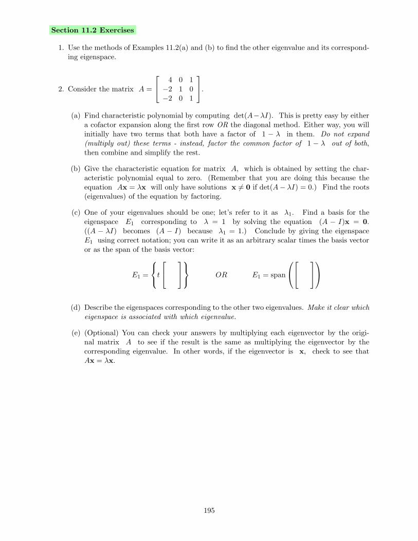
Section 11.2 Exercises
1. Use the methods of Examples 11.2(a) and (b) to find the other eigenvalue and its correspond-ing eigenspace.
2. Consider the matrix A =
4 0 1−2 1 0−2 0 1
.
(a) Find characteristic polynomial by computing det(A−λI). This is pretty easy by eithera cofactor expansion along the first row OR the diagonal method. Either way, you willinitially have two terms that both have a factor of 1 − λ in them. Do not expand(multiply out) these terms - instead, factor the common factor of 1 − λ out of both,then combine and simplify the rest.
(b) Give the characteristic equation for matrix A, which is obtained by setting the char-acteristic polynomial equal to zero. (Remember that you are doing this because theequation Ax = λx will only have solutions x 6= 0 if det(A− λI) = 0.) Find the roots(eigenvalues) of the equation by factoring.
(c) One of your eigenvalues should be one; let’s refer to it as λ1. Find a basis for theeigenspace E1 corresponding to λ = 1 by solving the equation (A − I)x = 0.((A − λI) becomes (A − I) because λ1 = 1.) Conclude by giving the eigenspaceE1 using correct notation; you can write it as an arbitrary scalar times the basis vectoror as the span of the basis vector:
E1 =
t
OR E1 = span
(d) Describe the eigenspaces corresponding to the other two eigenvalues. Make it clear whicheigenspace is associated with which eigenvalue.
(e) (Optional) You can check your answers by multiplying each eigenvector by the origi-nal matrix A to see if the result is the same as multiplying the eigenvector by thecorresponding eigenvalue. In other words, if the eigenvector is x, check to see thatAx = λx.
195

11.3 Diagonalization of Matrices
Performance Criterion:
11. (e) Diagonalize a matrix; know the forms of the matrices P and D fromP−1AP = D.
We begin with an example involving the matrix A from Examples 11.1(a) and (b).
⋄ Example 11.3(a): For A =
[
−4 −63 5
]
and P =
[
−1 −21 1
]
, find the product
P−1AP .
First we obtain P−1 =1
(−1)(1) − (1)(−2)
[
1 2−1 −1
]
=
[
1 2−1 −1
]
. Then
P−1AP =
[
1 2−1 −1
] [
−4 −63 5
] [
−1 −21 1
]
=
[
2 00 −1
]
We want to make note of a few things here:
• The columns of the matrix P are eigenvectors for A.
• The matrix D = P−1AP is a diagonal matrix.
• The diagonal entries of D are the eigenvalues of A, in the order of the correspondingeigenvectors in P .
For a square matrix A, the process of creating such a matrix D in this manner is calleddiagonalization of A. This cannot always be done, but often it can. (We will fret about exactlywhen it can be done later.) The point of the rest of this section is to see a use or two of this idea.
Before getting to the key application of this section we will consider the following. Supposethat we wish to find the kth power of a 2×2 matrix A with eigenvalues λ1 and λ2 and havingcorresponding eigenvectors that are the columns of P . Then solving P−1AP = D for A givesA = PDP−1 and
Ak = (PDP−1)k = (PDP−1)(PDP−1) · · · (PDP−1)
= PD(P−1P )D(P−1P ) · · · (P−1P )DP−1
= PDDD · · ·DP−1
= PDkP−1
= P
[
λ1 00 λ2
]k
P−1
= P
[
λk1 00 λk
2
]
P−1
Therefore, once we have determined the eigenvalues and eigenvectors of A we can simply takeeach eigenvector to the kth power, then put the results in a diagonal matrix and multiply once byP on the left and P−1 on the right.
196

⋄ Example 11.3(b): Diagonalize the matrix A =
3 12 −21−1 −6 130 −2 6
.
First we find the eigenvalues by solving det(A− λI) = 0:
det
3− λ 12 −21−1 −6− λ 130 −2 6− λ
= (3− λ)(−6− λ)(6 − λ)− 42 + 26(3 − λ) + 12(6− λ)
= (−18 + 3λ+ λ2)(6− λ)− 42 + 78− 26λ+ 72− 12λ
= −108 + 18λ+ 18λ− 3λ2 + 6λ2 − λ3 + 108− 38λ
= −λ3 + 3λ2 − 2λ
= −λ(λ2 − 3λ+ 2)
= −λ(λ− 2)(λ− 1)
The eigenvalues of A are then λ = 0, 1, 2. We now find an eigenvector corresponding toλ = 0 by solving the system (A− λI)x = 0. The augmented matrix and its row-reduced formare shown below:
3 12 −21 0−1 −6 13 00 −2 6 0
=⇒
1 0 5 00 1 −3 00 0 0 0
=⇒Let x3 = 1.Then x2 = 3and x1 = −5
The eigenspace corresponding to the eigenvalue λ = 0 is then the span of the vector v1 =[−5, 3, 1]. For λ = 1 we have
2 12 −21 0−1 −7 13 00 −2 5 0
=⇒
1 0 92 0
0 1 −52 0
0 0 0 0
=⇒Let x3 = 2.Then x2 = 5and x1 = −9
The eigenspace corresponding to the eigenvalue λ = 1 is then the span of the vector v2 =[−9, 5, 2] (obtained by multiplying the solution vector by two in order to get a vector with integercomponents). Finally, for λ = 2 we have
1 12 −21 0−1 −8 13 00 −2 4 0
=⇒
1 0 3 00 1 −2 00 0 0 0
=⇒Let x3 = 1.Then x2 = 2and x1 = −3
so the eigenspace corresponding to the eigenvalue λ = 2 is then the span of the vector v3 =[−3, 2, 1]. The diagonalization of A is then D = P−1AP , where
D =
0 0 00 1 00 0 2
and P =
−5 −9 −33 5 21 2 1
197

Section 11.3 Exercises
1. Consider matrix again the matrix A =
4 0 1−2 1 0−2 0 1
from Exercise 2 of Section 11.2.
(a) Let P be a matrix whose columns are eigenvectors for the matrix A. (The basis vectorsfor each of the three eigenspaces will do.) Give P and P−1, using your calculator tofind P−1.
(b) Find P−1AP , using your calculator if you wish. The result should be a diagonal matrixwith the eigenvalues on its diagonal. If it isn’t, check your work from Exercise 4.
2. Now let B =
0 0 −21 2 11 0 3
.
(a) Find characteristic polynomial by computing det(B − λI). If you expand along thesecond column you will obtain a characteristic polynomial that already has a factor of2− λ.
(b) Give the characteristic equation (make sure it has an equal sign!) for matrix B. Findthe roots (eigenvalues) by factoring. Note that in this case one of the eigenvalues isrepeated. This is not a problem.
(c) Find and describe (as in Exercise 1(c)) the eigenspace corresponding to each eigenvalue.The repeated eigenvalue will have TWO eigenvectors, so that particular eigenspace hasdimension two. State your results as sentences, and use set notation for the bases.
3. Repeat the process from Exercise 1 for the matrix B from Exercise 2.
198

11.4 Solving Systems of Differential Equations
Performance Criteria:
11. (f) Write a system of linear differential equations in matrix-vector form.Write the initial conditions in vector form.
(g) Solve a system of two linear differential equations; solve an initialvalue problem for a system of two linear differential equations.
We now get to the centerpiece of this section. Recall that the solution to the initial valueproblem x′(t) = kx(t), x(0) = C is x(t) = Cekt. Now let’s consider the system of twodifferential equations
x′1 = x1 + 2x2
x′2 = 3x1 + 2x2,
where x1 and x2 are functions of t. Note that the two equations are coupled; the equationcontaining the derivative x′1 contains the function x1 itself, but also contains x2. The samesort of situation occurs with x′2. The key to solving this system is to uncouple the two equations,and eigenvalues and eigenvectors will allow us to do that!
We will also add in the initial conditions x1(0) = 10, x2(0) = 5. If we let x =
[
x1x2
]
we can
rewrite the system of equations and initial conditions as follows:[
x′1x′2
]
=
[
1 2
3 2
] [
x1x2
]
,
[
x1(0)x2(0)
]
=
[
105
]
which can be condensed to
x′ = Ax, x(0) =
[
105
]
(1)
This is the matrix initial value problem that is completely analogous to x′(t) = kx(t), x(0) = C.
Before proceeding farther we note that the matrix A has eigenvectors
[
23
]
and
[
−11
]
with
corresponding eigenvalues λ = 4 and λ = −1. Thus, if P =
[
2 −13 1
]
we then have
P−1AP = D =
[
4 0
0 −1
]
and A = PDP−1.
We can substitute this last expression for A into the vector differential equation in (1) to getx′ = PDP−1x. If we now multiply both sides on the left by P−1 we get P−1x′ = DP−1x. Wenow let y = P−1x; Since P−1 is simply a matrix of constants, we then have y′ = (P−1x)′ =P−1x′ also. Making these two substitutions into P−1x′ = DP−1x gives us y′ = Dy. By thesame substitution we also have y(0) = P−1x(0). We now have the new initial value problem
y′ = Dy, y(0) = P−1x(0). (3)
Here the vector y is simply the unknown vector y =
[
y1y2
]
and y(0) =
[
y1(0)y2(0)
]
which can be
determined by y(0) = P−1x(0). Because the coefficient matrix of the system in (3) is diagonal,the two differential equations can be uncoupled and solved to find y. Now since y = P−1x wealso have x = Py, so after we find y we can find x by simply multiplying y by P .
So now it is time for you to make all of this happen!
199
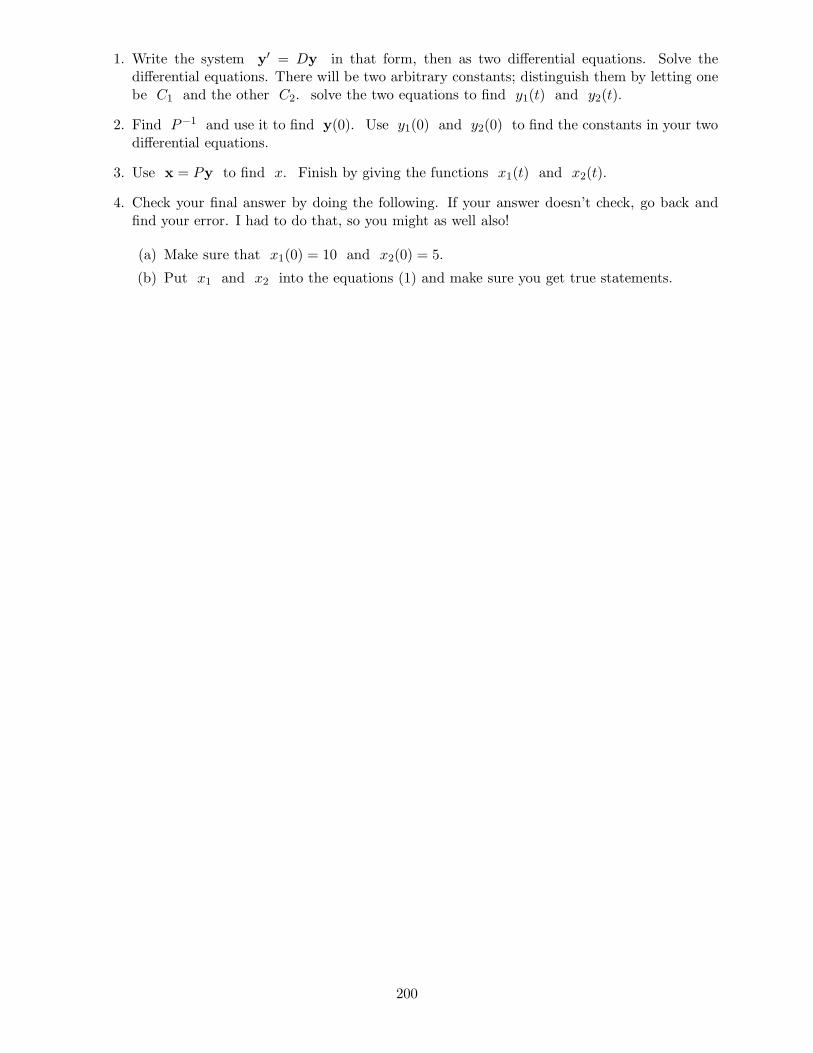
1. Write the system y′ = Dy in that form, then as two differential equations. Solve thedifferential equations. There will be two arbitrary constants; distinguish them by letting onebe C1 and the other C2. solve the two equations to find y1(t) and y2(t).
2. Find P−1 and use it to find y(0). Use y1(0) and y2(0) to find the constants in your twodifferential equations.
3. Use x = Py to find x. Finish by giving the functions x1(t) and x2(t).
4. Check your final answer by doing the following. If your answer doesn’t check, go back andfind your error. I had to do that, so you might as well also!
(a) Make sure that x1(0) = 10 and x2(0) = 5.
(b) Put x1 and x2 into the equations (1) and make sure you get true statements.
200
A Index of Symbols
R real number 7rref reduced row echelon form 10R2, R
3 two and three dimensional Euclidean space 33, 34a, b, c, x, y, z scalars 37u, vw,x vectors 37−−→OP position vector from the origin to point P 37−−→PQ vector from point P to point Q 37‖v‖ magnitude (or length) of vector v 38u · v dot product of u and v 56projvu projection of u onto v 57, 58A, B matrices 64AT transpose of a matrix 64A(i, j) ith row, jth column of matrix A 64In n× n identity matrix 64m× n dimensions of a matrix 64, 65aij i, jth entry of matrix A 65ai∗, a∗j ith row and jth column of matrix A 66Au matrix A times vector u 66AB product of matrices A and B 77A−1 inverse of the matrix A 81L lower triangular matrix 91U upper triangular matrix 91det(A) determinant of matrix A 95S a finite set of vectors 104col(A) column space of A 116null(A) null space of A 117x least squares solution 118e error vector for least squares approximation 120‖e‖ error for least squares approximation 120ej jth standard bassi vector 132B basis 132T, S transformations 146[T ] matrix for the linear transformation T 152S T composition of transformations S and T 154, 155λ, λj eigenvalues 160Ej eigenspace corresponding to eigenvalue λj 164P−1AP diagonalization of matrix A 166
201

202

B Solutions to Exercises
B.1 Chapter 1 Solutions
Section 1.2 Solutions
1. (a) (−2, 1) (b) (3, 4) (c) (3, 2)
(d) (1,−1) (e) (−1, 4) (f) (−2, 13)
2. (a) (4, 1) (b) (0,−3) (c) (2, 2)
Section 1.3 Solutions
1. The coefficient matrix is
1 1 −3−3 2 −12 1 −4
and the augmented matrix is
1 1 −3 1−3 2 −1 72 1 −4 0
2. Matrices A, B and D are in row-echelon form.
3. Matrices A and B are in reduced row-echelon form.
4.
1 1 −3 1−3 2 −1 72 1 −4 0
3R1 +R2 → R2
=⇒−2R1 +R3 → R3
1 1 −3 10 5 −10 100 −1 2 −2
5. (a)
1 5 −7 3−5 3 −1 04 0 8 −1
5R1 +R2 → R2
=⇒−4R1 +R3 → R3
1 5 −7 30 28 −36 150 −20 36 −13
(b)
2 −8 −1 50 −2 0 00 6 −5 2
=⇒3R2 +R3 → R3
2 −8 −1 50 −2 0 00 0 −5 2
(c)
1 −2 4 10 3 5 −20 2 −8 1
=⇒−2
3R2 +R3 → R3
1 −2 4 10 3 5 −20 0 −34
373
6. (a) (−4, 12 ,−4) (b) (33,−4, 1) (c) (7, 0,−2)
7. (a) (2, 3,−1) (b) (−2, 1, 2) (c) (−1, 2, 1)
8. Same as Exercise 7.
Section 1.4 Solutions
2. (a) y = −34x
2 + 52x− 3
4
3. (a) fourth degree (b) y = 25x+
2330x
2− 110x
3− 115x
4 or y = 0.4x+0.77x2−0.1x3−0.07x4
4. z = 3.765 + 0.353x − 1.235y
5. t1 = 52.6, t2 = 57.3, t3 = 61.6, t4 = 53.9, t5 = 57.1, t6 = 60.2
7. t1 = 44.6, t2 = 49.6, t3 = 38.6
203

B.2 Chapter 2 Solutions
Section 2.1 Solutions
1. (a) (6, 3, 4), (0, 0, 4), (−2,−1, 4), (2, 1, 4)(b) x− 2y = 0, z = 4, we can determine z (c) (2t, t, 4)
2. (a) y = 2t+ 2, x = t− 1
3. (a) no solution (b) (0,−2, t) (c) (7, t, 2) (d) no solution (e) (5, 3, 1)
(f) (−1, 2, 0) (g) (1− 2s+ t, s, t) (h) no solution (i) (2.5t− 4, t,−5)
4. t = −2: (5,−8,−2, 4), t = −1: (2,−3,−1, 4), t = 0: (−1, 2, 0, 4), t = 1: (−4, 7, 1, 4),t = 2: (−7, 12, 2, 4)
5. The leading variables are x and y, the free variable is z, and the rank of the coefficient matrixis two.
6. (t− 1, 2t+ 2, t), t = −1: (−2, 0,−1), t = 0: (−1, 2, 0), t = 1: (0, 4, 1), t = 2: (1, 6, 2)
There is no solution to the system with the next reduced matrix given.
(−2s + t+ 5, s, t,−4), s = t = 0: (5, 0, 0,−4), s = 1, t = 0: (3, 1, 0,−4),s = 0, t = 1: (6, 0, 1,−4)
Section 2.5 Solutions
1. (a) x1 = −1, x2 = 0
(b) x1 = t− 4, x2 = −2t+ 5, x3 = t, x4 = 2, (−4, 5, 0, 2), (−3, 3, 1, 2), (−2, 1, 2, 2),(−5, 7,−1, 2), etc.
(c) No solution
2. (a) (t− 13, t, 3, 4)
(b) (−14,−1, 3, 4), (−13, 0, 3, 4), (−12, 1, 3, 4), (−11, 2, 3, 4), (0, 13, 3, 4), (1, 14, 3, 4)(c) Change the 2 in the third row to a zero.
B.3 Chapter 3 Solutions
Section 3.1 Solutions
1. (a) Plane, intersects the x, y and z-axes at (3, 0, 0), (0, 6, 0) and (0, 0,−2), respectively.(b) Plane, intersects the x and z-axes at (6, 0, 0) and (0, 0, 2), respectively. Does not intersect
the y-axis.
(c) Plane, intersects only the y-axis, at (0,−6, 0).(d) Not a plane.
(e) Plane, intersects the x, y and z-axes at (−6, 0, 0), (0, 3, 0) and (0, 0,−2), respectively.
2. Any equation of the form ax + by = c, where c and at leat one of a or b is NOT zero. Theplane intersects the x-axis at ( c
a, 0, 0) if a 6= 0 and the z-axis at (0, 0, c
b) if b 6= 0.
3. y = 4
204

Section 3.2 Solutions
1. (a)−−→PQ = [17,−6,−15], ‖−−→PQ‖ =
√550 = 23.4
(b)−−→PQ = [12,−3], ‖−−→PQ‖ =
√153 = 12.4
(c)−−→PQ = [10,−1,−7, 9], ‖−−→PQ‖ =
√231 = 15.2
Section 3.3 Solutions
1. Tip-to-tail: Parallelogram:
−uv
v
−u+ 2v
−u
v
v
−u+ 2v
2.
[
−4530
]
3.
−c1 − 8c23c1 + c2−6c1 + 4c2
5. (a) v =
123
= 0
110
+ 2
011
+ 1
101
(b) v =
[
8−6
]
is any vector of the form (−12 t+
72 )
[
3−1
]
+ (12 t− 52)
[
11
]
+ t
[
1−1
]
6. (a) a1 =32 , a2 = 4, a3 = −1
2
(b) There are no such b1, b2 and b3
(c) det(A) = −42, det(B) = 0
Section 3.4 Solutions
2. (a) projbv =15− 2
25 + 4
[
5−2
]
=13
29
[
5−2
]
=
[ 6529
−2629
]
(b) projbv =10− 0
4 + 1
[
−21
]
= 2
[
−21
]
=
[
−42
]
(c) projbv =−6− 4
16 + 4
[
−2−4
]
= −1
2
[
−2−4
]
=
[
12
]
3.
projvu
(tail is where u and v meet)
u
v
(a)
projvu
uv
(b)
projvuu
v
(c)
u
(d)
205

B.4 Chapter 4 Solutions
Section 4.1 Solutions
1. (a) x
1
−32
+ y
1
2
1
+ z
−3−1−4
=
1
7
0
(b) x1
5
0
2
+ x2
0
2
1
+ x3
1
3
−4
=
−10
2
2. x
[
23
]
+ y
[
−3−1
]
=
[
−65
]
=⇒ 3
[
23
]
+ 4
[
−3−1
]
=
[
−65
]
[
23
]
[
−3−1
]
[
−65
]
3
[
23
]
=
[
69
]
4
[
−3−1
]
=
[
−12−4
]
[
−65
]
tip-to-tail method
3
[
23
]
=
[
69
]
4
[
−3−1
]
=
[
−12−4
]
[
−65
]
parallelogram method
206
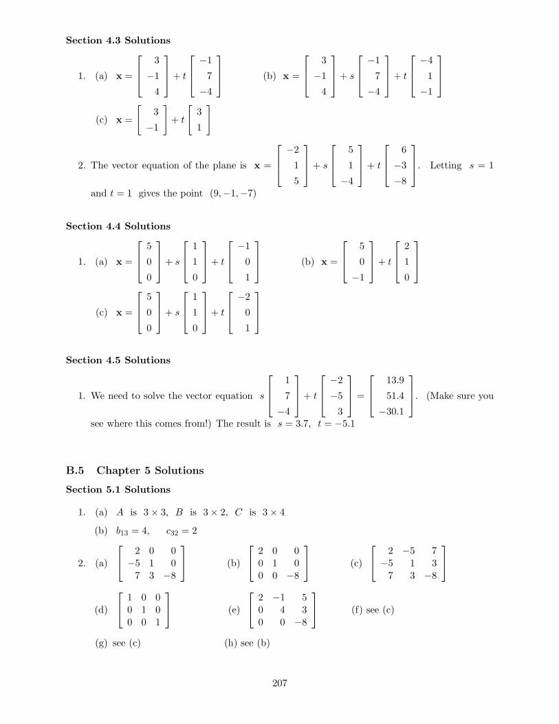
Section 4.3 Solutions
1. (a) x =
3
−14
+ t
−17
−4
(b) x =
3
−14
+ s
−17
−4
+ t
−41
−1
(c) x =
[
3
−1
]
+ t
[
3
1
]
2. The vector equation of the plane is x =
−21
5
+ s
5
1
−4
+ t
6
−3−8
. Letting s = 1
and t = 1 gives the point (9,−1,−7)
Section 4.4 Solutions
1. (a) x =
5
0
0
+ s
1
1
0
+ t
−10
1
(b) x =
5
0
−1
+ t
2
1
0
(c) x =
5
0
0
+ s
1
1
0
+ t
−20
1
Section 4.5 Solutions
1. We need to solve the vector equation s
1
7
−4
+ t
−2−53
=
13.9
51.4
−30.1
. (Make sure you
see where this comes from!) The result is s = 3.7, t = −5.1
B.5 Chapter 5 Solutions
Section 5.1 Solutions
1. (a) A is 3× 3, B is 3× 2, C is 3× 4
(b) b13 = 4, c32 = 2
2. (a)
2 0 0−5 1 07 3 −8
(b)
2 0 00 1 00 0 −8
(c)
2 −5 7−5 1 37 3 −8
(d)
1 0 00 1 00 0 1
(e)
2 −1 50 4 30 0 −8
(f) see (c)
(g) see (c) (h) see (b)
207

3. AT =
1 −3 40 1 75 −2 0
BT =
[
1 −3 40 1 7
]
CT =
1 −3 40 1 7−1 2 03 0 2
4. B +D =
2 −3−2 35 11
, B −D =
0 3−4 −13 3
, D −B =
0 −34 1−3 −3
Section 5.2 Solutions
1.
3−12
9
,
[
−2328
]
2. A =
[
3 −51 1
]
3. I3 =
1 0 00 1 00 0 1
, Ix = x
B.6 Chapter 6 Solutions
Section 6.1 Solutions
1.
[
2 −1−3 4
] [
4 15 −1
]
=
[
3 38 −7
]
2. A2 =
[
−15 5−3 −14
]
AF =
[
30 450 12
]
BC =
[
−69−25
]
BD =
[
62 −25 −2−121 80 36
]
CE =
−25 5 −1020 −4 8−35 7 −14
DC =
−5127−1
D2 =
39 3 18−48 18 −7
1 4 5
EC =[
−43]
ED =[
37 −2 13]
FA =
[
3 9−27 39
]
FB =
[
10 −35 106 147 −18
]
F 2 =
[
−2 −1166 75
]
3. The (2, 1) entry is −8 and the (3, 2) entry is −13.
4. a31a12 + a32a22 + a33a32 + a34a42 + a35a52
Section 6.3 Solutions
1. Since
[
2 53 8
] [
8 −4−3 2
]
=
[
1 20 4
]
6= I2, the matrices are not inverses.
2. (a) [I2 | B] =
[
1 0 −52
32
0 1 2 −1
]
(b) AB = BA = I2 (c) B is the inverse of A
208

Section 6.5 Solutions
1. (a) AT =
[
−5 0 21 4 −3
]
(b) ATA =
[
29 −11−11 26
]
, AAT =
26 4 −134 16 −12
−13 −12 13
(c) ATA and AAT are both square, symmetric matrices
2. For AB to not exist, B has to be a matrix with number of rows not equalling three. For ACto exist, C must have three rows.
3. If they are not square they can’t be inverses. If they are square, compute AB and see if it isthe identity matrix. If it is they are inverses; if it is not, they aren’t inverses.
4. (a) AB = I2
(b) The product BA doesn’t even exist, so it can’t be an identity matrix.
5.
[
2 −1 1 0−3 4 0 1
]
rref=⇒
[
1 0 0.36 0.090 1 0.27 0.18
]
so the inverse is
[
0.36 0.090.27 0.18
]
B.7 Chapter 7 Solutions
Section 7.1 Solutions
1.
a11 a12 a13a21 a22 a23a31 a32 a33
x1x2x3
=
a11x1 + a12x2 + a13x3a21x1 + a22x2 + a23x3a31x1 + a32x2 + a33x3
2. (a)
1 1 −3−3 2 −12 1 −4
x
y
z
=
170
(b)
[
5 −3 11 1 −7
]
x
y
z
=
[
−42
]
Section 7.3 Solutions
2. (a)
[
2 −34 5
] [
x1x2
]
=
[
43
]
(b) A−1 =1
10− (−12)
[
5 3−4 2
]
=1
22
[
5 3−4 2
]
(c)1
22
[
5 3−4 2
] [
2 −34 5
]
=1
22
[
22 00 22
]
=
[
1 00 1
]
(d)
[
2 −34 5
] [
x1x2
]
=
[
43
]
(e)
[
2 −3 1 04 5 0 1
]
1
22
[
5 3−4 2
]([
2 −34 5
] [
x1x2
])
=1
22
[
5 3−4 2
] [
43
] [
2 −3 1 00 11 −2 1
]
(
1
22
[
5 3−4 2
] [
2 −34 5
])[
x1x2
]
=1
22
[
5 3−4 2
] [
43
] [
2 −3 1 00 1 − 2
11111
]
[
1 00 1
] [
x1x2
]
=1
22
[
29−10
]
[
2 0 511
311
0 1 − 211
111
]
[
1 00 1
] [
x1x2
]
=
[
2922
−1022
] [
1 0 522
322
0 1 − 211
111
]
209

3. (a)
[
5 72 3
] [
x
y
]
=
[
−14
]
(b) A−1 =1
(5)(3) − (2)(7)
[
3 −7−2 5
]
=
[
3 −7−2 5
]
(c)
[
5 7 1 02 3 0 1
]
rref=⇒
[
1 0 3 −70 1 −2 5
]
, so A−1 =
[
3 −7−2 5
]
(d)
[
5 72 3
] [
x
y
]
=
[
−14
]
[
3 −7−2 5
]([
5 72 3
] [
x
y
])
=
[
3 −7−2 5
] [
−14
]
([
3 −7−2 5
] [
5 72 3
])[
x
y
]
=
[
−3122
]
[
1 00 1
] [
x
y
]
=
[
−3122
]
[
x
y
]
=
[
−3122
]
Section 7.4 Solutions
1. The determinant of the coefficient matrix is zero, so the system DOES NOT have a uniquesolution.
2. (a) If the determinant of A is zero, then the system has no solution or infinitely manysolutions.
(b) If the determinant of A is not zero, then the system has a unique solution.
3. (a) If the determinant of A is zero, then the system has infinitely many solutions. (It can’thave no solutions, because x = 0 is a solution.
(b) If the determinant of A is not zero, then the system has the unique solution x = 0.
Section 7.6 Solutions
1.
[
3 24 5
] [
x
y
]
=
[
−11
]
1
7
[
5 −2−4 3
]([
3 24 5
] [
x
y
])
=1
7
[
5 −2−4 3
] [
−11
]
(
1
7
[
5 −2−4 3
] [
3 24 5
])[
x
y
]
=1
7
[
−77
]
[
1 00 1
] [
x
y
]
=
[
−11
]
[
x
y
]
=
[
−11
]
2. (a)
[
15
]
,
[
3−2
]
,
[
−45
]
(b)
[
x1x2
]
,
[
1 35 −2
]
,
[
−45
]
210

B.8 Chapter 8 Solutions
Section 8.1 Solutions
1. (a) The span of the set is the x-axis.
(b) The span of the set is the xz-plane, or the plane y = 0.
(c) The span of the set is all of R2.
(d) The span of the set is the origin.
(e) The span of the set is a line through the origin and the point (1, 2, 3).
2. (a) w is not in the span of S. (b) w is not in the span of S.
(c)
838−1411
= −2
1−4−37
+ 5
26−45
(d)
37−4
= −4
100
+ 11
110
− 4
111
Section 8.3 Solutions
1. (a) Not a subspace, doesn’t contain the zero vector.
(b) Subspace. (c) Subspace.
(d) Not a subspace, the vector
−314
+
502
=
216
is not on either line because it
is not a scalar multiple of either vector.
(e) Not a subspace, the vector
123
is in the set, but −2
123
=
−2−4−6
is not.
(f) The set is a plane not containing the zero vector, so it is not a subspace.
(g) This is a plane containing the origin, so it is a subspace.
(h) The vector 0 is a subspace. (i) Subspace.
2. (a) The set is not a subspace because it does not contain the zero vector. We can tell thisbecause u and v are not scalar multiples of each other.
(b) The set is a subspace, and either of the vectors u or w by itself is a basis, as is anyscalar multiple of either of them.
Section 8.4 Solutions
1. (a) c1
12−1
+ c2
13−4
+ c3
0−26
=
2−917
,
1 1 0 22 3 −2 −9−1 −4 6 17
u1 is in the column space.
(b) −3
12−1
+ 5
13−4
=
2−917
.
211

(c) c1
12−1
+ c2
13−4
+ c3
0−26
=
3152
,
1 1 0 32 3 −2 15−1 −4 6 2
u2 is not in the column space.
2. v1 is in null(A) and v2 is not.
Section 8.6 Solutions
1. (a) Here the three vectors need to all be scalar multiples of each other.
(b) The span of two nonzero vectors that are not scalar multiples of each other is alwaysa plane, no matter what space we are in. If we create a linear combination of them inwhich neither is multiplied by zero we obtain another vector that is in the same plane,so the span does not increase when this new vector is included, yet the new vector is nota scalar multiple of either of the original two vectors.
(c) In order to have a chance of spanning R3, a set of vectors must contain at least three
vectors.
2. v1 =
[
15
]
, v2 =
[
210
]
and v3 =
[
41
]
would be one example. v1 and v2 must be
scalar multiples of each other, and v3 must NOT be a scalar multiple of either of them.
3. Any three vectors such that none is a scalar multiple of either of the other two, and that havethird components equal to zero, will do it.
B.9 Chapter 9 Solutions
Section 9.1 Solutions
1. (a) c1u1 + c2u2 + c3u3 = 0.
(b) The zero vector (in other words, c1 = c2 = c3 = 0) is a solution. If it is the ONLYsolution, then the vectors are linearly independent.
(c)−5c1 + 5c2 + 5c3 = 09c1 + 0c2 + 9c3 = 04c1 + 6c2 + 16c3 = 0
=⇒
−5 5 5 09 0 9 04 6 16 0
(d) c1 = −1, c2 = −2, c3 = 1 OR c1 = 1, c2 = 2, c3 = −1 OR any scalar multiple ofthese.
(e) u1 = −2u2 + u3, u2 = −12u1 +
12u3, u3 = u1 + 2u2
2. Solving c1
−134
+ c2
51−6
+ c3
−449
=
000
gives the general solution c1 = −32t,
c2 =12t, c3 = t. Therefore w = 3
2u− 12v. (Also u = 1
3v + 23w and v = 3u− 2w.)
212

3. For the following, use the vectors v1 =
13−1
, v2 =
1−24
, v3 =
14−2
.
(a) u is not in span(v1,v2,v3), but w is.
(b) −65v1 +
15v2 + v3 = 0. (c) v1 =
16v2 +
56v3.
Section 9.2 Solutions
1. (a) Not a subspace, doesn’t contain the zero vector.
(b) Subspace, a basis is
100
,
001
(c) Subspace, u is a basis.
(d) Not a subspace, the vector
−314
+
502
=
216
is not on either line because it
is not a scalar multiple of either vector.
(e) Not a subspace, the vector
123
is in the set, but −2
123
=
−2−4−6
is not.
(f) It can be shown that w, u and v are linearly independent, so the set is a plane notcontaining the zero vector, so it is not a subspace.
(g) This is a plane containing the origin, so it is a subspace. The set u,v is a basis.
(h) The vector 0 is a subspace. (i) All of R3 is a subspace.
2. (a) Not a subspace.
[
23
]
is in the set, but −1[
23
]
=
[
−2−3
]
.
(b) Subspace. A basis would be
100
,
011
.
Section 9.3 Solutions
2. (a) x1 = −4t, x2 = t and x3 = t. (b) x = t
−411
(c)
−411
3. A basis for the column space of A is
132
,
−115
.
4. (a) u1 is in the column space and u2 is not.
(b) A basis for col(A) is
12−1
,
13−4
. (c) u1 = −3
12−1
+5
13−4
.
5. (a) v1 is in null(A) and v2 is not.
213

(b) A basis for null(A) is
−221
. (c) v1 = −2
−221
.
6. The column space has dimension two and the null space has dimension one.
Section 9.5 Solutions
1. Solving c1
[
3−1
]
+ c2
[
11
]
+ c3
[
1−1
]
=
[
00
]
gives c1 = −12 , c2 =
12 and c3 = 1. We
can then write u2 = u1 − 2u3.
2. (a) Almost any three vectors in R3 will do, as long as no two are scalar multiples of each
other.
(b) Here we want three vectors where two of them are scalar multiples of each other.
3. (a) (i), (iii) (b) (ii) (c) (ii), (iii) (d) (ii)
(e) (i), (iii) (f) (i), (ii), (iii) (g) (ii) (h) (i), (iii)
(i) (ii) (j) (iii)
4. (a) The set is not a subspace because it does not contain the zero vector. We can tell thisbecause u and v are not scalar multiples of each other.
(b) The set is a subspace, and either of the vectors u or w by itself is a basis, as is anyscalar multiple of either of them.
(c) The set is a plane. When s = 0 and t = 12 , x is the zero vector, so the plane is a
subspace.
B.10 Chapter 10 Solutions
Section 10.2 Solutions
1. (a) T (u+ v) = T
([
u1u2
]
+
[
v1v2
])
= T
[
u1 + v1u2 + v2
]
=
u1 + v1 + 2(u2 + v2)3(u2 + v2)− 5(u1 + v1)
u1 + v1
=
=
u1 + 2u23u2 − 5u1
u1
+
v1 + 2v23v2 − 5v1
v1
= T
[
u1u2
]
+ T
[
v1v2
]
= T (u) + T (v)
(b) A =
1 2−5 31 0
2. (a) The transformation is linear.
(b) Not linear: T
(
2
[
35
])
= T
[
610
]
=
[
1660
]
and 2T
[
35
]
= 2
[
815
]
=
[
1630
]
,
so T
(
2
[
35
])
6= 2T
[
35
]
214

(c) Not linear: T
(
−2[
3−5
])
= T
[
−610
]
=
[
610
]
and −2T[
3−5
]
= −2[
35
]
=
[
−6−10
]
, so T
(
−2[
3−5
])
6= −2T[
3−5
]
(d) The transformation is linear.
3. (a) A =
[
0 11 1
]
(b) A =
[
3 01 −1
]
Section 10.4 Solutions
1. (a) Linear, A =
[
2 0 −11 1 1
]
(b) Not linear: T
123
+
456
= T
579
=
[
445
]
and T
123
+ T
456
=
[
51
]
+
[
264
]
=
[
315
]
, so T
123
+
456
6= T
123
+ T
456
2. (a) Linear, A =
1 0 10 1 11 1 0
(b) Not linear. Note that T
([
00
])
=
[
1−1
]
, which violates Theorem 10.2.2.
3. (a) A =
1 12 00 −3
, B =
[
5 −11 4
]
(b) (S T )[
x
y
]
= s
[
5x− y
x+ 4y
]
=
6x+ 3y10x− 2y−3x− 12y
(c) The matrix of S T is
6 310 −2−3 −12
(d) AB =
6 310 −2−3 −12
(e) The matrix of S T is AB.
215

Index
n-tuple, 8, 43LU-factorization, of a matrix, 1182-path, of a graph, 111
addition method, 5augment, a matrix, 107augmented matrix, 9
back substitution, 6basis, of a subspace, 160binary operation, 135
Cartesian plane, 44characteristic equation, 192characteristic polynomial, 192closed set, under an operation, 135codomain, of a function, 174coefficient matrix, 9cofactor expansion, 123column space, basis of, 164column space, of a matrix, 144column vector, 47, 83column, of a matrix, 9, 80components, of a vector, 47composition, of transformations, 184conditional statement, 141connected graph, 111conservation of flow, 31contrapositive, of a conditional statement, 141converse, of a conditional statement, 141counterexample, 139cross product, 55curve fitting, 14
dependent system, 24determinant, of a matrix, 123diagonal entries, of a matrix, 80diagonal matrix, 80diagonalization, of a matrix, 196digraph, 111dimension, of a subspace, 161dimensions, of a matrix, 9, 80directed edges, of a network, 31directed graph, 111direction vector, 71Dirichlet problem, 15domain, of a function, 174dot product, 55
edge, of a graph, 111eigenspace, 189, 194eigenvalue, 189eigenvector, 87, 189elements, of a set, 65entry, of a matrix, 9, 80error vector, 149Euclidean space, 43
forward-substitution, 118free variable, 24free variables, 26
Gauss-Seidel method, 34general solution, 27graph, 111
homogeneous system, of equations, 127hyperplane, 8, 76
identity matrix, 80, 87incidence graph, 111inconsistent system, 24infinite set, 65initial point, of a vector, 47inner product, 102, 104inverse, multiplicative, 106invertible matrix, 107iterative method, 33
Jacobi method, 33
leading entry, 10leading variables, 26least squares error, 149least squares solution, to a system of equations,
147length, of a vector, 47linear combination, 50linear combination form, of a system, 63linear combination form, of a system of equa-
tions, 63linear equation, 4linear operator, 85linear transformation, 176linear transformation, matrix of, 180linearity properties, 85linearly dependent, set of vectors, 155linearly independent, set of vectors, 155
216

lower triangular matrix, 80
magnitude, of a vector, 47matrix, 9, 80matrix equation form, of a system, 116method of least-squares, 30
nodes, of a network, 31norm, of a vector, 47null space, basis of, 164null space, of a matrix, 145nullity, of a matrix, 165
octant, 44operator, 84, 174ordered pair, 5ordered triple, 6orthogonal, 55outer product, 104overdetermined system of equations, 30
parallel vectors, 71parallelogram method, 50particular solution, 27path, in a graph, 111position vector, 47projection, 110projection matrix, 110projection, of one vector on another, 56
rank theorem, 166rank, of a matrix, 26, 165real number line, 44real numbers, 44reduced row-echelon form, 11resultant, 50rotation matrix, 87, 110row vector, 83row, of a matrix, 9, 80row-echelon form, 10row-reduction, 10
scalar quantity, 47set, 65solution to a system of linear equations, 4span, of a set of vectors, 130square matrix, 80standard basis, 160standard position, 47subspace, of R
n, 139substitution method, 5symmetric matrix, 81
system of linear equations, 4system, of differential equatoins, 199
tail, of a vector, 47target set, of a function, 174temperature equilibrium, 15terminal point, of a vector, 47tip, of a vector, 47tip-to-tail method, 50transformation, 174transpose of a matrix, 81trivial subspace, 141
unary operation, 135underdetermined system of equations, 30upper triangular matrix, 80
vector, 47, 48vector equation of a line, 71vector equation of a plane, 72vector form, of the solution to a system of equa-
tions, 74vector space, 137vertex, of a graph, 111
weighted average, 15whole numbers, 65
zero vector, 48
217