Ordinary Differential Equationsfor Engineers and Scientists

Gregg Waterman

Oregon Institute of Technology

c©2017 Gregg Waterman

This work is licensed under the Creative Commons Attribution 4.0 International license. The essence of the licenseis that

You are free to:

• Share copy and redistribute the material in any medium or format

• Adapt remix, transform, and build upon the material for any purpose, even commercially.

The licensor cannot revoke these freedoms as long as you follow the license terms.

Under the following terms:

• Attribution You must give appropriate credit, provide a link to the license, and indicate if changeswere made. You may do so in any reasonable manner, but not in any way that suggests the licensorendorses you or your use.

No additional restrictions You may not apply legal terms or technological measures that legally restrictothers from doing anything the license permits.

Notices:

You do not have to comply with the license for elements of the material in the public domain or where youruse is permitted by an applicable exception or limitation.

No warranties are given. The license may not give you all of the permissions necessary for your intendeduse. For example, other rights such as publicity, privacy, or moral rights may limit how you use the material.

For any reuse or distribution, you must make clear to others the license terms of this work. The best wayto do this is with a link to the web page below.

To view a full copy of this license, visit https://creativecommons.org/licenses/by/4.0/legalcode.

Contents

3 Second Order Linear ODEs 873.1 Homogeneous Second-Order Equations . . . . . . . . . . . . . . . . . . . . . . 903.2 Free, Undamped Vibration . . . . . . . . . . . . . . . . . . . . . . . . . . . . . 963.3 Free, Damped Vibration . . . . . . . . . . . . . . . . . . . . . . . . . . . . . . 1003.4 Particular Solutions, Part One . . . . . . . . . . . . . . . . . . . . . . . . . . . 1043.5 Differential Operators . . . . . . . . . . . . . . . . . . . . . . . . . . . . . . . 1083.6 Initial Value Problems and Forced, Damped Vibration . . . . . . . . . . . . . . 1133.7 Chapter 3 Summary . . . . . . . . . . . . . . . . . . . . . . . . . . . . . . . . 1163.8 Chapter 3 Exercises . . . . . . . . . . . . . . . . . . . . . . . . . . . . . . . . 118

D Solutions to Exercises 203D.3 Chapter 3 Solutions . . . . . . . . . . . . . . . . . . . . . . . . . . . . . . . . 203

i

3 Second Order Linear ODEs

Learning Outcome:

3. Solve second order linear, constant coefficient ODEs and IVPs. Understandthe nature of solutions to such ODEs and IVPs.

Performance Criteria:

(a) Solve an Euler equation.

(b) Solve a second order, linear, constant coefficient, homogeneous ODE.

(c) Set up and solve second order initial value problems modeling spring-masssystems and RLC circuits.

(d) Sketch or identify the graph of the solution to an IVP for an undampedmass on a spring with no forcing function.

(e) Write a function y = A sinωt + B cosωt in the alternate form y =C sin(ωt + φ). From this, determine the amplitude, period, frequency,angular frequency and phase shift.

(f) Determine from the coefficients of a second order, constant coefficienthomogeneous ODE whether the system it models is (i) underdamped,(ii) critically damped, (iii) overdamped, or (iv) undamped.

(g) Without finding the solution to the differential equation, sketch the graphof a solution of an overdamped or underdamped homogeneous secondorder, linear, constant coefficient ODE for given initial conditions. .

(h) Find a particular solution to a second order linear, constant coefficientODE using the method of undetermined coefficients.

(i) Evaluate a differential operator for a given function.

(j) Solve a second order linear, constant coefficient IVP.

(k) Identify the transient and steady-state parts of the solution to a dampedsystem with forced vibration.

In this course we are focusing on differential equations that can be solved by analytical (“pencil-and-paper”) techniques. Many differential equations cannot be solved this way, and numerical methods mustbe employed to obtain solutions. (See Appendix B for an introduction to solving ODEs by numericaltechniques.) Our chances of being able to solve an ODE analytically are much greater if it is linear.

A second order linear ODE has the form

a2(x)d2y

dx2+ a1(x)

dy

dx+ a0(x)y = f(x), (1)

and when f(x) = 0 it is a homogeneous linear differential equation. Here a2, a1 and a0 arefunctions of the independent variable x. In this chapter we will focus almost entirely on second orderlinear differential equations in which all the coefficients are constants and the independent variable istime t, rather than x. So our equations will generally have the form

ay′′ + by′ + cy = f(t), (2)

87

where a 6= 0, b and c are constants and f is a function that we will refer to as the forcing function.(2) is called a second order, linear, constant coefficient ODE. Recall that (1) and (2) are homogeneouswhen f = 0 for all x or t.

The one other type of (linear) equation we will see in this chapter is a variety called an Eulerequation. For such equations a2(x) = ax2, a1(x) = bx and a0(x) = c, where b and c areconstants, and f(x) = 0. Thus an Euler equation is one with the form

ax2d2y

dx2+ bx

dy

dx+ cy = 0 (3)

Equations of this form arise when solving certain partial differential equations. In the first section of thechapter we will solve equations of the forms

ax2d2y

dx2+ bx

dy

dx+ cy = 0 and ay′′ + by′ + cy = 0, (4)

both of which are clearly homogeneous. These equations will always have two solutions y1 and y2,and the general solution will be a linear combination

y = C1y1 + C2y2 (5)

of the two solutions. (C1 and C2 are of course constants.) It should at this point be no surprise thatthe general solution to equations of either of the forms (4) contain two arbitrary constants!

Our main focus as the chapter goes on will be solving initial value problems of the form

ay′′ + by′ + cy = f(t), y(0) = y0, y′(0) = y′0, (6)

with a, b and c being constants, a 6= 0. In addition, the initial values y0 and y′0 are constantsas well. The method we will use to solve the IVP will consist of four steps:

(1) We will first solve the homogeneous equation obtained by replacing f(t) with zero. This willgive us a solution of the form (5), called the homogenous solution. We will denote it by yh.

(2) Next we’ll find something called a particular solution, denoted by yp, for the ODE in (6). Wewill do this by a method called the method of undetermined coefficients.

(3) The general solution to the equation ay′′ + by′ + cy = f(t) is

y = yh + yp = C1y1(t) + C2y2(t) + yp(t), (7)

the sum of the homogenous solution and the particular solution.

(4) The initial conditions y(0) = y0 and y′(0) = y′0 are used to determine the values of theconstants C1 and C2. This gives us the final solution to the initial value problem (6).

Initial value problems of the form

ay′′ + by′ + cy = f(t), y(0) = y0, y′(0) = y′0, (6)

model certain electrical circuits and simple mechanical vibration. We will proceed through a seriesof variations on this initial value problem, developing an understanding of how the particular modeldescribes the system and how the solution y(t) behaves:

88

• In Section 1.2 we saw how a system consisting of a mass on a spring is modeled by the secondorder ODE

md2y

dt2= −ky or m

d2y

dt2+ ky = 0,

which is ay′′+ by′+ cy = f(t) with b = 0 and f(t) = 0. When b = 0 we refer to the systemas undamped, and when f(t) = 0 the system is free. We begin our study of applications withfree, undamped systems in Section 3.2.

• In Section 3.3 we will add damping, but still no forcing function. That is, we’ll have b 6= 0 andf(t) = 0. In this case we’ll see that there are three possible scenarios - the system is just one of(a) underdamped, overdamped, or critically damped. In Section 3.3 we will also introduce anelectrical circuit for which the mathematical model is exactly the same as a mass on a spring.

• Next, in Section 3.4, we will consider systems that are both damped (so b 6= 0 and forced (sof(t) 6= 0). We will see in that section how to find particular solutions to forced systems.

• Differential operators are introduced in Section 3.5. These give us a convenient way to understandthe nature of solutions to forced systems.

• In Section 3.6, we’ll put together everything from the previous sections to solve initial valueproblems with second order, linear, constant coefficient differential equations. We’ll consider suchIVPs in applied settings, and we’ll examine the nature of solutions to such IVPs.

As a specific example of an ODE of the form ay′′ + by′ + cy = f(t), let’s consider

y′′ + 5y′ + 6y = 5 sin 3t.

We want to know not only how to solve such ODEs and their associated IVPs, but also to know whatkind of behavior to expect from solutions, based on the original ODE or IVP. Here is a summary of someof the ideas you will run across, which were previously brought up in Chapter 2:

• The left hand side of the ODE represents some sort of “system” like a mass on a spring or asimple electric circuit. The function on the right represents some kind of input to the system,which we call a forcing function, since it forces movement (for a mass on a spring) or current(for an electrical circuit) in the system.

• The solution function y is the response of the system, and will often consist of exponential ortrigonometric functions, or products of the two. The solution may have several terms, some ofwhich may “die out” (go to zero) as time goes on, and others that may not. The parts that dieout are called transient parts of the solution, and parts that are constant or periodic are calledsteady-state parts. These are also referred to as the transient and steady-state response of thesystem.

89

3.1 Homogeneous Second-Order Equations

Performance Criterion:

3. (a) Solve an Euler equation.

(b) Solve a second order, linear, constant coefficient, homogeneous ODE.

In this section we will solve second order homogeneous equations of the forms

ax2d2y

dx2+ bx

dy

dx+ cy = 0 and ay′′ + by′ + cy = 0, (1)

where a 6= 0, b and c are constants. In both cases, solutions are obtained by guessing what the generalform of a solution might be and then substitution that guess into the ODE and “making it work.” Thefirst equation in (1) is called an Euler equation and the second is a second order, linear, constantcoefficient, homogeneous ODE. The bulk of this chapter is about constant coefficient equations. Inthis section we’ll first see how to solve Euler equations, then look at homogeneous constant coefficientequations, whose solutions take a variety of forms.

Consider the Euler equationx2y′′ + 2xy′ − 6y = 0.

Note that if y was some power of x then y′ would be one power lower and y′′ two powers lower.If we then substituted our y, y′ and y′′ into the ODE we would have three terms of the same powerdue to the multiplication of y′ by x and y′′ by x2 in the ODE. Thus there might be some hopethat the three terms add up to zero.

⋄ Example 3.1(a): Solve the ODE x2y′′ + 2xy′ − 6y = 0 by guessing a solution of the formy = xp and determining the value of p.

Solution: First we compute y′ = pxp−1 and y′′ = p(p − 1)xp−2. Substituting these into theODE we get

x2p(p− 1)xp−2 + 2xpxp−1 − 6xp = 0

p(p− 1)xp + 2pxp − 6xp = 0

xp[

p(p− 1) + 2p − 6]

= 0

xp(p2 + p− 6) = 0

Now the quantity xp is only zero when x = 0, leading to the trivial solution y = 0. Becausewe would like nonzero solutions, it must be the case that p2 + p − 6 = 0. Solving this givesus p = −3, 2, so both y = x−3 and y = x2 are solutions. The general solution is theny = C1x

−3 + C2x2.

We now contemplate the second order linear, constant coefficient, homogeneous ODE

y′′ + 5y′ + 6y = 0.

In this case we are looking for some function y = y(t) (we will be interested in applications inwhich time is the independent variable) for which we can multiply the function and its first and second

90

derivatives by constants, add the results and get zero. This indicates that y must essentially be equalto its first and second derivatives, which only occurs for exponential functions. Therefore we guess thatthe solution has the form y = ert, where r is some constant.

⋄ Example 3.1(b): Solve y′′ + 5y′ + 6y = 0, assuming that the independent variable is t.

Solution: We substitute the guess y = ert into the ODE, resulting in

r2ert + 5rert + 6ert = (r2 + 5r + 6)ert = 0

Now the quantity ert is never zero, so r2 + 5r + 6 = 0. Solving this gives us r = −3,−2, soboth y = e−3t and y = e−2t are solutions. It is not hard to show that if y1 and y2 are bothsolutions to a homogeneous ODE and C1 and C2 are constants, then y = C1y1 + C2y2 isalso a solution. So in this case, the general solution is y = C1e

−3t + C2e−2t.

When using the above method to solve

ay′′ + by′ + cy = 0 (2)

we will arrive at (ar2 + br + c)ert = 0, leading to ar2 + br + c = 0. We will refer to the equationar2 + br + c = 0 as the auxiliary equation (also called the characteristic equation) associated withthe ODE ay′′ + by′ + cy = 0, and we will call solutions to this equation roots of the equation. Thefollowing summarizes what we saw in the above example, which is only one of several possible formsthat a solution to (2) can take.

When the auxiliary equation for a second order, linear, constant coefficient homo-geneous equation has two real roots r1 and r2, the solution to the ODE is

y = C1er1t +C2e

r2t.

Video Example - watch from 1:20 to 3:10

The most efficient method for finding the roots of the auxiliary equation r2 + 5r + 6 = 0 fromExample 3.1(b) is to factor the left side, but we could have used the quadratic formula

r =−b±

√b2 − 4ac

2a(2)

instead. We will at times want or need to use the quadratic formula, and at other times factoring oranother method may be more efficient for finding the roots of the auxiliary equation. Regardless of whatwe might do in practice, an examination of (2) is useful for determining the various possibilities whenobtaining the roots to the auxiliary equation:

• When b2 − 4ac > 0 there will be two real roots, as in Example 3.1(b).

• When b2 − 4ac = 0 there will only be one real root, which is a rather special case.

• When b2 − 4ac < 0 and b 6= 0 the roots will be complex conjugates. That is, they will becomplex numbers of the form r = k + λi and r = k − λi, where i =

√−1.

91

• When b2 − 4ac < 0 and b = 0, the roots will be two purely imaginary numbers r = λi andr = −λi. (This is just the previous case, with k = 0.)

Video Discussion

Each of the above cases results in different forms of the solution to the homogeneous equationay′′ + by′ + cy = 0, and the methods for solving the auxiliary equations are generally different as well,although the quadratic formula could be used in all cases. We’ve already taken care of the first casewith Example 3.1(b).

We now consider the second case above. Suppose that we were to try the method of Example 3.1(b)for the ODE y′′ + 6y′ + 9y = 0. We would only get one value for r, −3. By the same reasoningas used before we then have the solution y = C1e

−3t +C2e−3t; because these are like terms, this can

be written y = Ce−3t, where C = C1 + C2. But (for reasons we’ll go into in more depth later) thegeneral solution to a second order ODE must be the sum of two “different” functions, each multipliedby arbitrary constants, so something is wrong! The following example shows that there is in fact anothersolution besides e−3t.

⋄ Example 3.1(c): Verify that y = te−3t is also a solution to the ODE y′′ + 6y′ + 9y = 0.

Solution: Using the product and chain rules to compute the derivatives,

y′ = t(e−3t)′ + t′e−3t = −3te−3t + e−3t

y′′ = −3(te−3t)′ − 3e−3t = −3(−3te−3t + e−3t)− 3e−3t = 9te−3t − 6e−3t

Substituting into the ODE,

y′′ + 6y′ + 9y =(

9te−3t − 6e−3t)

+ 6(

− 3te−3t + e−3t)

+ 9(

te−3t)

= 9te−3t − 6e−3t − 18te−3t + 6e−3t + 9te−3t

= 0

The general solution to the ODE y′′ + 6y′ + 9y = 0 is then y = C1e−3t + C2te

−3t. Any timethat our auxiliary equation has a repeated root r (both solutions are the same), one of the solutionsis ert, and the other solution is tert. We’ll see in Section 4.2 how this solution is obtained.

When the auxiliary equation for a second order, linear, constant coefficient homo-geneous equation has only one real root r, the solution to the ODE is

y = C1ert + C2te

rt.

Video Example

We now consider the case where b2 − 4ac < 0 and b = 0, resulting in two purely imaginaryroots r = ±λi. We’ll consider the homogeneous equation y′′ + 9y = 0 that we looked at previously,which can be rewritten as y′′ = −9y. Through our familiarity with derivatives and the chain rule, weguessed (correctly) that both y = sin 3t and y = cos 3t are solutions, and it is not hard to show that

92

y = C1 sin 3t + C2 cos 3t is a solution. Now how would it work to try the method of Example 3.1(b)for this equation? Letting y = ert we have

y′′ + 9y = r2ert + 9ert = (r2 + 9)ert = 0

so we need to solve r2+9 = 0 ⇒ r2 = −9. If we allow complex solutions, the solution to this equationis r = ±3i, so the solution to the ODE is y = Ae3it + Be−3it, where A and B are arbitrayconstants. (We could have used C1 and C2 for the constants as we have been doing, but we are“saving” them, as you’ll see.) To continue we will need the following:

Euler’s Formula: eiθ = cos θ + i sin θ

To see where Euler’s Formula comes from, see Appendix B.5. We will also use the two basic trigidentities:

cos(−θ) = cos θ, sin(−θ) = − sin θ

Combining the two solutions e3it and e−3it, we get

y = Ae3it +Be−3it

= A(

cos 3t+ i sin 3t)

+B[

cos(−3t) + i sin(−3t)]

= A cos 3t+Ai sin 3t+B cos 3t−Bi sin 3t

= (A+B) cos 3t+ (A−B)i sin 3t

= C1 cos 3t+ C2 sin 3t.

Here A and B are constants, and C1 = A+B, C2 = (A−B)i. Now it seems that C2 should bea complex number, which is a bit disconcerting. However, it is possible that A and B are complexas well, in such a way that perhaps C2 turns out to be real! You will find that this method “works,”regardless. The following summarizes what we have just seen.

When the auxiliary equation for a second order, linear, constant coefficient homoge-neous equation has two purely imaginary roots r = ±λi, the solution to the ODEis

y = C1 sinλt+ C2 cos λt.

Let’s use a specific example to examine the final situation, where the auxiliary equation has twocomplex roots r = k ± λi.

⋄ Example 3.1(d): Solve y′′ + 10y′ + 28y = 0.

Solution: Guess y = ert, so y′ = rert and y′′ = r2ert. Then

y′′ + 10y′ + 28y = r2ert + 10rert + 28ert = (r2 + 10r + 28)ert = 0

Again, ert cannot equal zero, so we solve r2+10r+28 = 0; this is done in this case using thequadratic formula:

r =−10±

√

102 − 4(28)

2= −5± 2i

√2

93

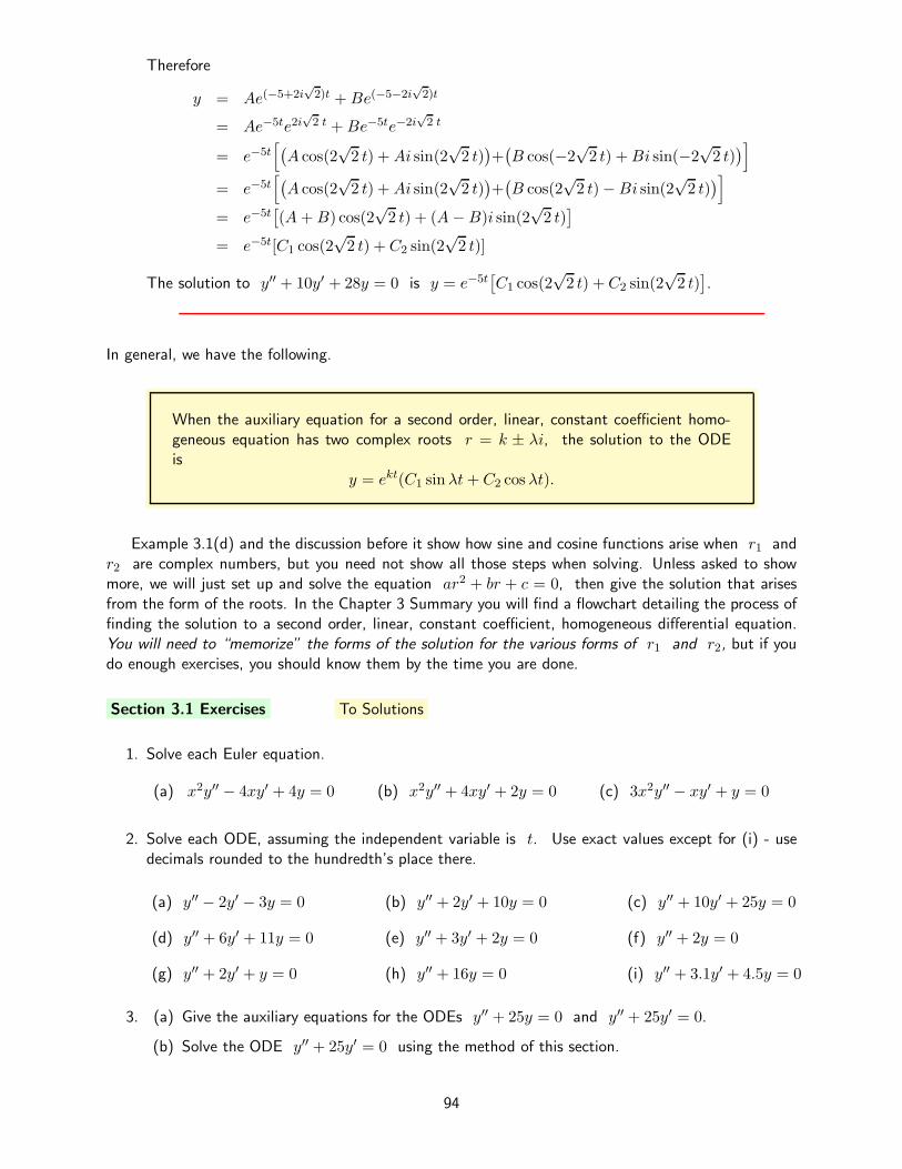
Therefore

y = Ae(−5+2i√2)t +Be(−5−2i

√2)t

= Ae−5te2i√2 t +Be−5te−2i

√2 t

= e−5t[

(

A cos(2√2 t) +Ai sin(2

√2 t)

)

+(

B cos(−2√2 t) +Bi sin(−2

√2 t)

)

]

= e−5t[

(

A cos(2√2 t) +Ai sin(2

√2 t)

)

+(

B cos(2√2 t)−Bi sin(2

√2 t)

)

]

= e−5t[

(A+B) cos(2√2 t) + (A−B)i sin(2

√2 t)

]

= e−5t[C1 cos(2√2 t) + C2 sin(2

√2 t)]

The solution to y′′ + 10y′ + 28y = 0 is y = e−5t[

C1 cos(2√2 t) +C2 sin(2

√2 t)

]

.

In general, we have the following.

When the auxiliary equation for a second order, linear, constant coefficient homo-geneous equation has two complex roots r = k ± λi, the solution to the ODEis

y = ekt(C1 sinλt+ C2 cos λt).

Example 3.1(d) and the discussion before it show how sine and cosine functions arise when r1 andr2 are complex numbers, but you need not show all those steps when solving. Unless asked to showmore, we will just set up and solve the equation ar2 + br + c = 0, then give the solution that arisesfrom the form of the roots. In the Chapter 3 Summary you will find a flowchart detailing the process offinding the solution to a second order, linear, constant coefficient, homogeneous differential equation.You will need to “memorize” the forms of the solution for the various forms of r1 and r2, but if youdo enough exercises, you should know them by the time you are done.

Section 3.1 Exercises To Solutions

1. Solve each Euler equation.

(a) x2y′′ − 4xy′ + 4y = 0 (b) x2y′′ + 4xy′ + 2y = 0 (c) 3x2y′′ − xy′ + y = 0

2. Solve each ODE, assuming the independent variable is t. Use exact values except for (i) - usedecimals rounded to the hundredth’s place there.

(a) y′′ − 2y′ − 3y = 0 (b) y′′ + 2y′ + 10y = 0 (c) y′′ + 10y′ + 25y = 0

(d) y′′ + 6y′ + 11y = 0 (e) y′′ + 3y′ + 2y = 0 (f) y′′ + 2y = 0

(g) y′′ + 2y′ + y = 0 (h) y′′ + 16y = 0 (i) y′′ + 3.1y′ + 4.5y = 0

3. (a) Give the auxiliary equations for the ODEs y′′ + 25y = 0 and y′′ + 25y′ = 0.

(b) Solve the ODE y′′ + 25y′ = 0 using the method of this section.

94

4. Give the general form of the solution (that is, give one of the forms found in the boxes in thissection) to ay′′ + by′ + cy = 0 under each of the following conditions:

(a) b = 0 (b) b2 − 4ac > 0 (c) b2 − 4ac < 0, b 6= 0 (d) b2 − 4ac = 0

5. (a) Solve the Euler equation x2y′′ − 3xy′ + 4y = 0. You should obtain only one solution.

(b) We know that there should be two solutions. Show that y = x2 lnx, x > 0, is also asolution.

95

3.2 Free, Undamped Vibration

Performance Criteria:

3. (c) Set up and solve second order initial value problems modeling spring-masssystems and RLC circuits.

(d) Sketch or identify the graph of the solution to an IVP for an undampedmass on a spring with no forcing function.

(e) Write a function y = A sinωt + B cosωt in the alternate form y =C sin(ωt + φ). From this, determine the amplitude, period, frequency,angular frequency and phase shift.

Let’s return to the following example:

⋄ Example 1.1(a): Suppose that a mass is hanging on a springthat is attached to a ceiling, as shown to the right. If we lift themass, or pull it down, and let it go, it will begin to oscillate upand down. Its height (relative to some fixed reference, like itsheight before we lifted it or pulled it down) varies as time goeson from when we start it in motion. We say that height is a

function of time.

spring

mass

In Section 1.2 we derived the differential equation

md2y

dt2+ ky = 0 (1)

that governs the motion of the mass. Here y is the height (from equilibrium) of the mass at any timet after it is set in motion by some means, with positive being upward. m is the mass of the mass(the first of these being a quantity, and the second being an object) and k is the spring constant. Wewill assume that there is no external force acting on the mass once it is set in motion - in such caseswe call the vibration free. We will also consider the system to be undamped, which means that thereis nothing hindering the motion of the mass once it begins moving up and down.

First let’s remind ourselves of how we can solve such ODEs:

⋄ Example 3.2(a): Solve Equation 1 for a mass of 10.3 and a spring constant of 28.7 (both with

appropriate units).

Solution: The auxiliary equation corresponding to the ODE is 10.3r2 + 28.7 = 0. Subtracting28.7 from both sides and dividing by 10.3 gives r2 = −2.786.... If we then take the square rootof both sides and round to the nearest hundredth, we have r = ±1.67i. Therefore the solutionto the ODE is y = C1 sin 1.67t + C2 cos 1.67t.

96

Intuitively it is reasonable that, once set in motion, amass on a spring with no damping will oscillate forever withthe same amplitude. The graph of such motion would looksomething like what is shown to the right; this is referred toas harmonic motion. It may not be clear how the solutionto the above differential equation, which contains a sum ofsine and cosine functions, gives a graph like the one shown.We’ll soon see a computation that makes it clear how thishappens.

y (in)

t (sec)

A mass hanging on a spring can be set in motion by doing one of three things:

• moving the mass away from its equilibrium position and letting it go

• giving the mass some initial velocity upward or downward from its initial position

• moving the mass away from its initial position and giving it an initial velocity

If we move the mass upward or downward, that will give y(0) equal to some value other than zero,and if we impart an initial velocity the value of y′(0) will be nonzero.

⋄ Example 3.2(b): Suppose that the mass from Example 3.2(a) is set in motion by lifting it upone inch and giving it an initial velocity of 2 inches per second downward, both at time zero. Givethe initial conditions in function form and sketch a graph of what you expect the motion to looklike. Then determine the solution to the initial value problem and graph it to check your graph.

Solution: The condition of raising the mass up by oneinch is given by y(0) = 1, and the initial velocity of twoinches per second downward is given by y′(0) = −2,with the negative indicating that the velocity is in thedownward direction. Because the mass starts above itsequilibrium point, we expect the y-intercept of the graphto be at positive one. The condition of being given aninitial velocity downward means that the slope of thetangent line to the graph at t = 0 will be negative.We therefore expect a graph something like that shownto the right.

y (in)

t (sec)

1

Applying the first initial condition with the solution from Example 3.2(a) gives C2 = 1. Takingthe derivative of the solution obtained in Example 3.2(a) gives

y′ = 1.67C1 cos 1.67t − 1.67C2 sin 1.67t.

Substituting the initial velocity initial condition and C2 = 1 into this gives us C1 = −1.20 (thezero indicates accuracy to the hundredth’s place), so the solution to the IVP is

y = −1.20 sin 1.67t + cos 1.67t.

The graph of this function agrees with that shown above.

It is sometimes useful to change an expression of the form −1.20 sin 1.67t+cos 1.67t into a singlesine function with a phase shift, and here is what we use to do it:

97

C sin(ωt+ φ) Form

A sinωt+B cosωt = C sin(ωt+ φ), where C =√

A2 +B2

and φ = tan−1 B

Aif A > 0, φ = π + tan−1 B

Aif A < 0

If A = 0, then B cosωt = B sin(

ωt+ π2

)

Note that radian mode must be used when using a calculator to compute φ!

⋄ Example 3.2(c): Change the solution y = −1.20 sin 1.67t + cos 1.67t into the form y =

C sin(ωt+ φ), where C, ω and φ are all decimals rounded to the hundredth’s place.

C =√

(−1.20)2 + 12 = 1.56, φ = π + tan−1 B

A= 2.44

Thus the solution can be written as y = 1.56 sin(1.67t + 2.44).

We see that the amplitude of the motion for the situation from Examples 3.2(a), (b) and (c) is 1.56,greater than the initial position of one unit. That is due to the initial velocity - you will see in theexercises what happens if there is no initial velocity.

There are some important parameters associated with a function y = C sin(ωt+ φ):

Amplitude, frequency, period and phase shift

For a function y = C sin(ωt+ φ),

• C is the amplitude • ω is the angular frequency

• T =2π

ωis the period • f =

1

T=

ω

2πis the frequency

• −φ

ωis the phase shift • ω = 2πf

⋄ Example 3.2(d): For the function y = 1.56 sin(1.67t + 2.44), give the amplitude, period,frequency and phase shift.

Solution: The amplitude is 1.56, the period is T =2π

1.67= 3.76, the frequency is f =

1

T=

0.64 and the phase shift is −2.44

1.67= −1.46.

With a bit of careful thought, the following should be clear: Only the amplitude and and phase shift

are influenced by the initial conditions. The period, frequency and angular frequency in this case are alldetermined by m and k, the parameters of the system.

98

Section 3.2 Exercises To Solutions

1. Suppose that the mass is set in motion by moving it upward by 2.5 cm and releasing it with noinitial velocity.

(a) Sketch what you think the graph of y versus t will look like, taking care with the factthat positive y is upward. Make the amplitude of the motion clear on your graph.

(b) Express the initial conditions mathematically by giving values for y(0) and y′(0).

2. Repeat Exercise 1 for a mass that is set in motion by hitting it upward (as it hangs at equilibrium),giving it an initial speed of 3 inches per second.

3. Repeat Exercise 1 for a mass that is set in motion by giving it an initial speed of 8 cm per seconddownward from a point 2 cm above equilibrium. The amplitude is not two - make it clear whetherit is more or less than two.

4. A mass of 34 is attached to a spring with a spring constant of 15. It is set into motion by

raising it 2.5 cm and releasing it. (See Exercise 1.)

(a) Set up an initial value problem consisting of a differential equation and two initial conditions.

(b) Solve the initial value problem to find the position function y. Give all numbers as decimals,rounded to the hundredth’s place.

(c) Graph your solution using some technology and compare with your answer to Exercise 1.They should agree; if they don’t, figure out what is wrong and fix it!

(d) Put your solution in the form C sin(ωt + φ). Graph the resulting function and make surethe graph agrees with what you got for (c). If not, try to find and correct your error.

(e) Give the amplitude, angular frequency, period, frequency and phase shift of the solution.

5. (a) Consider again a mass of 34 attached to a spring with a spring constant of 15, as in

Exercise 4. Solve the initial value problem obtained with the initial conditions of Exercise3, where the initial speed was 8 cm downward from a point 2 cm above equilibrium. Againgive all numbers as decimals, rounded to the hundredth’s place.

(b) Graph your solution using technology and compare with your answer to Exercise 3.

(c) Put your solution in the form y = A sin(ωt+φ). Check it by graphing it and your solutionto part (a) together; they should be the same!

(d) Give the amplitude, angular frequency, period, frequency and phase shift of the solution.

6. A mass of 410 on a spring with spring constant 4 is given an initial velocity of 9 cm/sec upward

from an initial position of 4 cm below equilibrium.

(a) Give the initial value problem.

(b) Find the equation of motion of the mass, y(t), in the form y = A sin(ωt+ φ).

(c) Give the amplitude, angular frequency, period, frequency and phase shift of the solution.

99

3.3 Free, Damped Vibration

Performance Criteria:

3. (c) Set up and solve second order initial value problems modeling spring-masssystems and RLC circuits.

(f) Determine from the coefficients of a second order, constant coefficienthomogeneous ODE whether the system it models is (i) underdamped,(ii) critically damped, (iii) overdamped, or (iv) undamped.

(g) Without finding the solution to the differential equation, sketch the graphof a solution of an overdamped or underdamped homogeneous secondorder, linear, constant coefficient ODE for given initial conditions.

Consider again a mass on a spring, but suppose that we submerge themass in an oil bath, as shown to the right (think about an oil-dampedshock absorber). As the mass moves up and down there is now anadditional force acting on it, the resistance of the oil. We will make theassumption that the force is directly proportional to the velocity but inthe opposite direction; that is, for some positive constant β (the Greek

letter beta), the force of resistance is given by −βdy

dt.

oil

Suppose that we also have some variable external force acting on the mass as well. (Think forceexerted upward on a shock absorber by the road, as a car drives along.) If this force is some functionf(t), then the net force on the mass at any time t is

Fnet = md2y

dt2= f(t)− β

dy

dt− ky.

If we rearrange this equation we get

md2y

dt2+ β

dy

dt+ ky = f(t), (1)

the second order differential equation that models the motion of a spring-mass system with dampingand an external forcing function f .

Now suppose that we have an electric circuit consisting of a re-sistor, an inductor and a capacitor in series with each other, alongwith (perhaps) a voltage source. We will refer to such a circuit asan RLC circuit, shown schematically to the right. The differen-tial equation that models an RLC circuit is derived from Kirchoff’svoltage law which tells us that the sum of the voltage drops acrosseach of the three components is equal to the voltage imposed onthe system by the voltage source. By Ohm’s law the voltage dropacross the resistor is V = iR, where i is the current and R isthe resistance of the resistor.

E

R

L

C

Figure 3.1

100

The voltage drops across the inductor and the capacitor are Ldi

dtand

1

Cq, where q is the charge

on the capacitor. From Kirchoff’s voltage law we now have

Ldi

dt+Ri+

1

Cq = E(t), (2)

where E(t) is the voltage as a function of time. (It may of course be constant, such as in the case ofDC voltage supplied by a battery.)

But the current i is the rate at which charge is passing by a point in the circuit: i =dq

dtThus

di

dt=

d

dt

(

dq

dt

)

=d2q

dt2and the above equation becomes

Ld2q

dt2+R

dq

dt+

1

Cq = E(t) , (3),

where L is the inductance of the inductor in henries, R is the resistance of the resistor in ohms, andC is the capacitance of the capacitor in farads. All are positive quantities; this will be important! Ifwe would rather work with current rather than charge we can differentiate both sides of (3) to get

Ld2i

dt2+R

di

dt+

1

Ci = E′(t) , (4),

Note that both (3) and (4) are completely analogous to equation (1), which models a spring-masssystem. This illustrates the principle, first encountered in Section 2.5, that different physical situationsare often modeled by the same differential equation.

In this section we will consider the situation in which there is no forcing function. That is, the righthand sides of (1), (3) and (4) are zero. Of course something needs to happen to get the mass moving orto get current to flow in the circuit, and each can be accomplished in a variety of ways. For example, thespring and the capacitor both have the ability to store energy by compressing or stretching the spring,or by storing charge in the capacitor (with the positivity or negativity of that charge being analogousto compressing or stretching the spring). As that energy is released it will cause the mass to move orcurrent to flow in the circuit. Here is a summary of initial conditions we can have for the spring, whichwe previously gave in Section 3.2:

• the mass can be displaced and let go, with no initial velocity

• the mass can be given some velocity at its resting position

• the mass can be displaced AND given some initial velocity upward or downward

The analogous conditions for the electric circuit are as follows:

• there is no current in the circuit, but there is an initial charge on the capacitor

• there is no charge on the capacitor, but there is an initial current

• there is both an initial charge on the capacitor and an initial current

Our main objective in this section is to understand the behavior of the solution function y(t) ofequation (1), (3) or (4) when f(t) = 0 or E(t) = 0, and how that behavior varies depending on theparameters m, k and β or R, L and C. You will be looking at some exercises to do this. Realizethat the values given for the parameters may not be realistic - they were chosen in such a way as tomake the mathematics reasonable.

101

Section 3.3 Exercises To Solutions

For all exercises in this section you will be working with the equation

md2y

dt2+ β

dy

dt+ ky = f(t), (1)

for various values of m, β and k, but always with f(t) = 0.

1. (a) Solve the initial value problem consisting of Equation (1) with m = 5, β = 6 andk = 80, and initial conditions y(0) = 2, y′(0) = −6. Give your answer in the formy = Ceat sin(ωt+φ) and all numbers in decimal form, rounded to the nearest tenth. (Notethat 5.0007 rounded to the nearest tenth is 5.0, not 5! What is the difference?)

(b) Graph the solution to the IVP on your calculator. Adjust the viewing window to get aboutthree cycles of the motion displayed fairly large. Sketch your graph.

(c) Graph y = 2.3e−0.6t and y = −2.3e−0.6t together with the solution you graphed in (b).Add them to your sketch as dashed curves.

What you have just seen is an example of what is called underdamped vibration. There is damping,but it is small enough to allow the mass to move up and down while the vibration decays.

2. (a) Solve the initial value problem consisting of Equation (1) with m = 5, β = 50 and k = 80,and initial conditions y(0) = 2, y′(0) = 6.

(b) Sketch the graph of your solution over a time period long enough to show what is happeningover time. Make your vertical scale such that the general shape of the graph can be seen.

(c) Compare and contrast your solution to this IVP with the solution to the IVP from Exercise1, in terms of amplitude over time and oscillation.

For your answer to 2(c) you should have noted that the solution of the IVP in Exercise 1 oscillates as itdecays, and the solution of the IVP in Exercise 2 does not. We say that the situation from Exercise 2 isoverdamped vibration. The initial conditions do not affect whether the vibration will be underdampedor overdamped (can you see why not?), so the only difference is the value of β.

3. (a) Determine a value of β that is the “dividing line” between equations have solutions thatoscillate as they decay and those that do not oscillate. Explain how you determined it.

(b) Solve the IVP with m = 5, k = 80 and the value of β you obtained in (a), along withthe initial conditions from Exercise 2. Graph the solution using some technology and sketchthe graph.

(c) Suppose now that m = 5 and k = 80. How would you expect the solution to (1) tobehave if β was slightly smaller than the value obtained in (a), and why. How would youexpect the solution to behave for β slightly larger than the value obtained in (a)? Answerthese questions in complete sentences.

For your answer to 3(c) you should have said that if β is a little less than the value that you found in(a) the solution will behave like that in Exercise 1, and if β is a little more than that value the solutionwill behave like that in Exercise 2. The situation in Exercises 3(a) and 3(b) is called the criticallydamped case, meaning that if there is just a little less damping the behavior will be oscillatory, but ifthe damping has that critical value or greater, the motion will not be oscillatory.

4. Describe a method for determining from the coefficients m, β and k whether the solution willbe underdamped, overdamped, or critically damped.

102

5. Sketch the graph of the solution to a 2nd-order, constant-coefficient homogeneous ODE with thegiven damping conditions and initial conditions.

(a) Underdamped, y(0) < 0, y′(0) > 0.

(b) Overdamped, y(0) < 0, y′(0) < 0.

(c) Overdamped, y(0) > 0, y′(0) < 0. (I think there may be a couple different appearancespossible here - we’ll investigate this more later.)

(d) Undamped (not underdamped, but undamped), y(0) > 0, y′(0) > 0.

6. Consider a circuit like that shown in Figure 3.1, but without the voltage source E = 0. Thecomponents are a 0.15 henry inductor, a 500 ohm resistor and a 2× 10−5 farad capacitor, theinitial charge on the capacitor is 1.3 × 10−6 coulombs and there is no initial current. (This canbe achieved by having an open switch in the circuit and closing the switch at time zero.)

(a) Is the system overdamped, underdamped, or critically damped?

(b) Use equation (3) to determine the charge on the capacitor at any time t. Round allconstants to three significant figures and give correct units with your answer.

(c) If you didn’t already in part (b), put your answer in y = Cekt sin(ωt+ φ) form.

(d) Give the current in the circuit at any time t, again giving units with your answer androunding to two significant digits.

103

3.4 Particular Solutions, Part One

Performance Criteria:

3. (h) Find a particular solution to a second order linear, constant coefficientODE using the method of undetermined coefficients.

In the previous section we found out how to solve equations of the form

ay′′ + by′ + cy = f(t) (1)

when f(t) = 0, but in practice we are usually interested in situations where f(t) 6= 0. For thosesituations we will use a technique called the method of undetermined coefficients to find a solution.To do this we (again!) substitute a guess, which we will call the trial particular solution, into the ODE.This trial solution will contain one or more unknown constants, whose values can be determined byfinding the result obtained when the trial solution is substituted into the left hand side of the ODE andthen setting it equal to the known right hand side f(t). Like terms are then equated, and the constantsdetermined. The resulting solution is called the particular solution to (1). Later we will see how theparticular solution is combined with the homogeneous solution to give the general solution to (1).

Let’s consider the ODEy′′ + 9y = 5e−2t.

If y had the form y = Ae−2t for some constant A, then y′′ would have the same form. Perhapsthere is then a choice of A for which y′′ + 9y will equal 5e−2t. The next example shows us that isin fact the case.

⋄ Example 3.4(a): Find a value A for which y = Ae−2t is a solution to y′′ + 9y = 5e−2t.

Solution: First we observe that

y = Ae−2t =⇒ y′ = −2Ae−2t =⇒ y′′ = 4e−2t.

Substituting these into the left side of (1) we get

y′′ + 9y = 4Ae−2t + 9Ae−2t = 13Ae−2t.

We now set this equal to the right hand side of the ODE to get 13Ae−2t = 5e−2t. The only waythat this can be true is if the coefficients of e−2t are equal: 13A = 5 ⇒ A = 5

13 . Thereforey = 5

13e−2t is a solution to y′′ + 9y = 5e−2t.

A particular solution to a differential equation is any solution that does not contain arbitrary constants,so y = 5

13e−2t is a particular solution to the ODE y′′ + 9y = 5e−2t. We sometimes subscript the

dependent variable with the letter p to indicate a particular solution. For the above we would thenwrite yp =

513e

−2t. This distinction is made because, as we will soon see, there are other solutions aswell.

Next we will examine the ODE y′′ + 7y′ + 10y = 5t2 − 8. We might guess that the particularsolution will be a fourth degree polynomial, because then y′′ would be a second degree polynomial. Itturns out that there is no harm in trying a fourth degree polynomial (you will try it in the exercises),but in fact a second degree polynomial is adequate. The next example demonstrates this.

104

⋄ Example 3.4(b): Find the coefficients A, B and C for which yp = At2 + Bt + C is a

solution to y′′ + 7y′ + 10y = 5t2 − 8.

Solution: First we compute the needed derivatives:

yp = At2 +Bt+C =⇒ y′p = 2At+B =⇒ y′′p = 2A.

Next we substitute these values into the left side of the ODE and group by powers of t:

y′′p + 7y′p + 10yp = 2A+ 7(2At+B) + 10(At2 +Bt+ C)

= 2A+ 14At+ 7B + 10At2 + 10Bt+ 10C

= 10At2 + (14A + 10B)t+ (2A+ 7B + 10C)

Setting this equal to the right hand side of the ODE gives us

10At2 + (14A + 10B)t+ (2A + 7B + 10C) = 5t2 + 0t− 8,

and equating coefficients of powers of t (including the constant term) results in the threeequations

10A = 5, 14A+ 10B = 0, 2A+ 7B + 10C = −8.

From the first equation we see that A = 12 . Substituting that value into the second equation

and solving for B results in B = − 710 . Finally, when we substitute the values we have found for

A and B into the last equation and solve for C we get C = − 41100 . The particular solution

to y′′ + 7y′ + 10y = 5t2 − 8 is then

yp =12 t

2 − 710t−

41100 .

It is important to note that even though the right hand side 5t2 − 8 contains only a t2 term and aconstant term, we need to include a t term in our guess for the particular solution. If we had insteadguessed a particular solution of the form yp = At2 + B and substituted it into the ODE we wouldhave obtained the two equations

10A = 5 and 14A = 0,

both of which cannot be true at the same time!So far we have found a particular solution to ay′′ + by′ + cy = f(t) when f(t) is an exponential

function (Example 3.4(a)) and a polynomial (Example 3.4(b)). The only other type of function we willconsider for f(t) is a trigonometric function; suppose we have the ODE

y′′ + 4y′ + 3y = 5 sin 2t. (2)

Based on what we have seen so far, our first inclination might be that we should consider a particularsolution of the form yp = A sin 2t. Let’s try it:

yp = A sin 2t =⇒ y′p = 2A cos 2t =⇒ y′′p = −4A sin 2t

soy′′p + 4y′p + 3yp = −4A sin 2t+ 8A cos 2t+ 3A sin 2t

= −A sin 2t+ 8A cos 2t.

Here we need A = 0 because there is no cosine term on the right hand side of (2), but then we’d haveno sine term either!

So what do we do? Well, the “trick” is to let yp have both sine and cosine terms even though theright side of the ODE has only a sine term.

105

⋄ Example 3.4(c): Determine values for A and B so that yp = A sin 2t + B cos 2t is the

particular solution to y′′ + 4y′ + 3y = 5 sin 2t.

Solution: We see that

y′p = 2A cos 2t− 2B sin 2t, y′′p = −4A sin 2t− 4B cos 2t.

soy′′p + 4y′p + 3yp = (−4A sin 2t− 4B cos 2t)

+ 4(2A cos 2t− 2B sin 2t) + 3(A sin 2t+B cos 2t)

= (−A− 8B) sin 2t+ (8A−B) cos 2t

Thus, in order for the left hand side to equal the right hand side, it must be the case that8A − B = 0 because there is no cosine term in the right hand side, and −A − 8B = 5, sothat the sine terms are equal. Solving the first equation for B and substituting into the secondequation results in A = − 1

13 . Substituting this back into the second equation gives B = − 813 .

Our particular solution is then yp = − 113 sin 2t−

813 cos 2t.

At this point we have the following guesses for a particular solution to a differential equation of theform ay′′ + by′ + cy = f(t) when using the method of undetermined coefficients:

• If f is a polynomial of degree n, then

yp = Antn +An−1t

n−1 + · · ·+A2t2 +A1t+A0

Note that all powers of t less than or equal to the degree of f(t) are included.

• If f(t) = Cekt, then yp = Aekt.

• If f(t) = C1 sin kt+ C2 cos kt, then yp = A sin kt + B cos kt. Even if one of C1 or C2 is

zero, the trial yp must still contain both the sine and cosine terms.

In Section 4.3 we will see that there is a bit more to be added to this story, but for now the abovesummarizes what we have seen so far.

Section 3.4 Exercises To Solutions

1. For each of the following, give the form the particular solution must have.

(a) y′′ + 3y′ + 2y = 5t− 1 (b) y′′ + 6y′ + 9y = cos 2t

(c) y′′ + 9y = 2e5t (d) y′′ − 4y′ − 5y = 6 sin t

(e) 2y′′ + 3y′ + y = 7 (f) y′′ + 3y = 2t+ 3e−t

2. Determine the particular solution for each of the ODEs in Exercise 1.

3. Suppose that you thought that the ODE y′′+3y′+2y = 5t−1 should have a particular solutionof yp = At3 + Bt2 + Ct + D. (Note that this is the ODE from Exercise 1(a).) Substitutethis into the ODE and see what happens for this guess. Does it give you the correct particularsolution?

106

4. You would think that the particular solution to y′′ + 3y′ + 2y = 6e−t would have the formyp = Ae−t, but that is not the case. In Section 4.3 we will see what our guess for the particularsolution should be. For now, try substituting the given particular solution into the ODE to seewhat happens.

5. Solve each of the following homogeneous ODEs, assuming the independent variable for each is t.

(a) y′′ + 4y′ + 29y = 0 (b) 2y′′ + 11y′ + 5y = 0

(c) y′′ + 6y′ + 9y = 0 (d) y′′ + 3y = 0

107

3.5 Differential Operators

Performance Criterion:

3. (i) Evaluate a differential operator for a given function.

An Example

In this section we will begin by exploring a specific second order ODE in order to illustrate someideas we will capitalize on in order to solve linear, constant coefficient, second order ODEs. The ODEthat we will be considering is

y′′ + 9y = 5e−2t, (1)

which we found to have a particular solution of yp =513e

−2t. (See Example 3.1(a).) This was obtainedby substituting a guess of y = Ae−2t for y in y′′ + 9y and setting the result equal to 5e−2t. Thefollowing example shows that y = 5

133−2t is not the only solution to (1).

⋄ Example 3.5(a): Show that y = C sin 3t+ 513e

−2t, where C is any constant, is a solution to

the differential equation (1).

Solution: Taking derivatives we get

y′ = 3C cos 3t− 10133

−2t and y′′ = −9C sin 2t+ 2013e

−2t.

Substituting in to the left hand side of the ODE we get

y′′ + 9y = −9C sin 2t+ 2013e

−2t + 9(C sin 3t+ 513e

−2t)

= −9C sin 2t+ 2013e

−2t + 9C sin 3t+ 4513e

−2t)

= 6513e

−2t

= 5e−2t

Thus y = C sin 3t+ 513e

−2t is a solution to y′′ + 9y = 5e−2t.

To examine further what is going on here it is convenient to develop some terminology and notation.

Differential Operators

A function can be thought of as a “mathematical machine” that takes in a number and, in return,gives out a number. There are other mathematical machines that take in things other than numbers,like functions or vectors, usually giving out things like what they take in. These sorts of “machines”are often referred to as operators. A simple example of an operator that you are quite familiar with isthe derivative operator. When we take the derivative of a function, the result is another function. To

indicate the action of a derivative on a function y = y(t) we will writedy

dtas

d

dt(y),

108

which is like the function notation f(x), with ddt

taking the place of f and y taking the place ofx. The derivative operator has a very special property that you should be familiar with from calculus.If a and b are any constants and y1 and y2 are functions of t, then

d

dt(ay1 + by2) =

d

dt(ay1) +

d

dt(by2) = a

d

dt(y1) + b

d

dt(y2). (2)

Operators that “distribute over addition” and “pass through constants” like this are called linear op-erators.

You might guess that the second derivative, and other higher derivatives, are linear operators as well,and that is correct. We are particularly interested in operators that are created by multiplying a functionand some of its derivatives by constants and adding them all together. It is customary to denote such

operators with the letter D, for differential operator. An example would be D = 3d2

dt2+ 5

d

dt− 4,

whose action on a function y = y(t) is defined by

D(y) = 3d2y

dt2+ 5

dy

dt− 4y. (3)

Let’s look at a specific example of how this operator works.

⋄ Example 3.5(b): For the operator D defined by (3), find D(y) when y = t2 − 3t.

Solution: D(y) = 3d2

dt2(t2 − 3t) + 5

d

dt(t2 − 3t)− 4(t2 − 3t)

= 3(2) + 5(2t − 3)− 4(t2 − 3t)

= 6 + 10t− 15− 4t2 + 12t

= −4t2 + 22t− 9

When we combine several mathematical objects by multiplying each by a constant and adding (orsubtracting) the results, we obtain what is called a linear combination of those objects. The operatorD defined by (3) is a linear combination of a function and its first two derivatives. (We can think ofthe function itself as the “zeroth derivative,” making all the things being combined derivatives.) Youhave seen linear combinations in other contexts; any polynomial function like

f(x) = 3x4 − 7x3 +1

3x2 − x+ 5.83

is a linear combination of 1, x, x2, x3, x4,... . Those of you who have had a course in linear algebrahave seen linear combinations of vectors.

Again, we can think of an operator as a machine that takes in afunction and gives out some resulting function that is based somehowon the input function. This is illustrated to the right for Example 3.5(b).The next example demonstrates that a differential operator formed as alinear combination of derivatives is a linear operator.

D

t2 − 3t

−4t2 + 22t− 9

⋄ Example 3.5(c): Show that the operator D defined by

D(y) = 3d2y

dt2+ 5

dy

dt− 4y

109

is a linear operator by showing that it satisfies (2).

Solution: To determine whether D is linear we need to apply it to ay1 + by2:

D(ay1 + by2) = 3d2

dt2(ay1 + by2) + 5

d

dt(ay1 + by2)− 4(ay1 + by2)

= 3

(

ad2y1

dt2+ b

d2y2

dt2

)

+ 5

(

ady1

dt+ b

dy2

dt

)

− 4ay1 − 4by2

= 3ad2y1

dt2+ 3b

d2y2

dt2+ 5a

dy1

dt+ 5b

dy2

dt− 4ay1 − 4by2

= 3ad2y1

dt2+ 5a

dy1

dt− 4ay1 + 3b

d2y2

dt2+ 5b

dy2

dt− 4by2

= a

(

3d2y1

dt2+ 5

dy1

dt− 4y1

)

+ b

(

3d2y2

dt2+ 5

dy2

dt− 4y2

)

= aD(y1) + bD(y2)

Because D(ay1 + by2) = aD(y1) + bD(y2), D is a linear operator.

At the second line above we have applied the fact that the first and second derivative are linear operators.With a bit of thought it should be clear that this, along with the distributive property, is what makes alinear combination of derivatives a linear operator.

Back to the Example

We return now to considering the ODE

y′′ + 9y = 5e−2t, (1)

for which we have shown that both

y = 513e

−2t and y = C sin 3t+ 513e

−2t (4)

are solutions. If we now let D be the operator defined by D(y) = y′′ + 9y, then (4) says that

D(

513e

−2t)

= 5e−2t and D(

C sin 3t+ 513e

−2t)

= 5e−2t.

Looking a little more closely, we see that

D(

C sin 3t)

=d2

dt2

(

C sin 3t)

+ 9(

C sin 3t)

= −9C sin 3t+ 9C sin 3t = 0.

This explains why D applied to the sum of C sin 3t and 513e

−2t is a solution; by linearity ofdifferential operators,

D(

y1 +513e

−2t)

= D(

y1)

+D(

513e

−2t)

= 0 + 5e−2t = 5e−2t

for any function y1 for which D(

y1)

= 0 (like C sin 3t, for example). This gives us the following:

110

Let D be a linear differential operator with independent variable t. If y2 is asolution to D(y2) = f(t) and y1 is a solution to D(y1) = 0, then it is also thecase that D(y1 + y2) = f(t).

The general form of equation that we are most interested in is

ay′′ + by′ + cy = f(t), (5)

where a, b and c are constants. Our goal is to find a general solution to this equation, meaning asolution that encompasses all possible solutions. Such a solution will consist of a particular solution to(5) that contains no arbitrary constants plus the family of all possible solutions to

ay′′ + by′ + cy = 0. (6)

The solution to (5) without arbitrary constants is of course the particular solution to the equation,and the family of all possible solutions to (6) is the homogeneous solution. We saw in Section 3.1how to find the homogeneous solution yh and in Section 3.2 we saw how to find the particular solutionyp. The general solution is then y = yh + yp.

As an example, we know that the ODE

y′′ + 9y = 5e−2t

has homogeneous solution yh = C1 sin 3t + C2 cos 3t and particular solution yp = 513e

−2t, so thegeneral solution is

y = yh + yp = C1 sin 3t+ C2 cos 3t+513e

−2t.

For reasons you will see in Section 4.3, we will always find the homogeneous solution first and then theparticular solution.

Section 3.5 Exercises To Solutions

1. Let the differential operator D be defined on a function y = y(t) by

D(y) =d2

dt2(y) + 3

d

dt(y) + 2y.

Find D(y) for each of the following functions y.

(a) y = t2 + 7t (b) y = 5e−2t (c) y = 5cos 2t (d) y = 52 t−

174

2. What does your answer to Exercise 1(d) tell us about the ODE y′′ + 3y′ + 2y = 5t− 1?

3. Although you don’t realize why at this point, your answer to Exercise 1(b) is somewhat special.

(a) Does the same thing happen for y = Ce−2t, where C is some constant other than 5? Ifso, for what value or values of C?

(b) Does the same thing happen if y = ekt, where k is some constant other than −2? Ifso, for what value or values of k?

111

4. Let the differential operator D be defined on a function y = y(t) by

D(y) =d2

dt2(y) + 6

d

dt(y) + 9y.

Find D(y) for each of the following functions y.

(a) y = e−3t (b) y = te−3t (c) y = 5e−3t − 2te−3t

5. Let S be an operator on functions. S is linear if

S(af + bg) = aS(f) + bS(g), (7)

where a and b are any constants and f and g are any functions of the sort that S can acton. (7) is equivalent to the two separate conditions that

S(af) = aS(f) and S(f + g) = S(f) + S(g), (8)

where a, f and g are as before. That is, if both conditions in (8) hold for S, then it is a linearoperator. Now let’s define a specific operator S by S(f(t)) = f(t) + 3 for any function f(t).

(a) What is S(cos t)? S(t2 + 5t− 1)?

(b) What is S(4 cos t)? What is 4S(cos t)? Are both results the same? What does that tellus about S, in terms of linearity?

(c) Find S(cos t+ e2t) and S(cos t) + S(e2t).

112

3.6 Initial Value Problems and Forced, Damped Vibration

Performance Criteria:

3. (j) Solve a second order linear, constant coefficient IVP.

(c) Set up and solve second order initial value problems modeling spring-masssystems and RLC circuits.

(k) Identify the transient and steady-state parts of the solution to a dampedsystem with forced vibration.

Now that we know how to find the general solution to ay′′ + by′ + cy = f(t) we are ready to solveinitial value problems whose ODEs are of this form. Here is how the process goes:

Solving the IVP ay′′ + by′ + cy = f(t), y(0) = y0, y′(0) = y′0

1) Find the homogeneous solution yh to ay′′ + by′ + cy = 0.

2) Use the method of undetermined coefficients to find the particular solutionyp of the ODE ay′′ + by′ + cy = f(t).

3) Construct the general solution y = yh + yp.

4) Apply the initial conditions to the general solution to find the values of thearbitrary constants.

We have already covered the first three steps of the above. It is very important to remember thatthe initial conditions are applied to the general solution to find the values of the arbitrary constants.A common mistake by students is to find the values of the constants based on only the homogeneoussolution - this is incorrect.

Let’s look at an example:

⋄ Example 3.6(a): Solve the IVP

y′′ + 4y′ + 3y = 5 sin 2t, y(0) = 2, y′(0) = −1

Solution: We must first solve the homogeneous equation y′′ + 4y′ + 3y = 0. The rootsof the auxiliary equation are r1 = −1 and r2 = −3 (of course it doesn’t matter which iswhich), so the homogeneous solution is yh = C1e

−t + C2e−3t. Our trial particular solution is

yp = A sin 2t+B cos 2t. This gives us

y′p = 2A cos 2t− 2B sin 2t, y′′p = −4A sin 2t− 4B cos 2t.

so

LHS = (−4A sin 2t− 4B cos 2t) + 4(2A cos 2t− 2B sin 2t) + 3(A sin 2t+B cos 2t)

= (−A− 8B) sin 2t+ (8A−B) cos 2t

113

Thus, in order for the left hand side to equal the right hand side, it must be the case that8A − B = 0 because there is no cosine term in the right hand side, and −A − 8B = 5, sothat the sine terms are equal. Solving the first equation for B and substituting into the secondequation results in A = − 1

13 . Substituting this back into the second equation gives B = − 813 .

Our particular solution is then yp = − 113 sin 2t−

813 cos 2t, and the general solution is

y = yh + yp = C1e−t + C2e

−3t − 113 sin 2t−

813 cos 2t

The derivative of the general solution is

y′ = −C1e−t − 3C2e

−3t − 213 cos 2t+

1613 sin 2t

Applying the initial conditions gives us the two equations

C1 +C2 − 813 = 2 and − C1 − 3C2 − 2

13 = −1

Adding these and solving for C2 gives us C2 = −2326 . Substituting this into either equation

gives C1 =9126 . The solution to the IVP is then

y = 9126e

−t − 2326e

−3t − 113 sin 2t−

813 cos 2t

It is often the case that finding the constants C1 and C2 comes down to solving a system of twoequations in two unknowns, as it did here.

Section 3.6 Exercises To Solutions

1. You may have found the particular solution to each of the following ODEs in Exercise 2 of Section3.4. Give the general solution to each.

(a) y′′ + 3y′ + 2y = 5t− 1 (b) y′′ + 6y′ + 9y = 5cos 3t

(c) y′′ + 9y = 2e5t (d) y′′ − 4y′ − 5y = 6 sin t

(e) 2y′′ + 3y′ + y = 7 (f) y′′ + 3y = 2t+ 3e−t

2. Solve each of the following IVPs by the process described in the box at the start of the section.

(a) y′′ + 9y = 4 sin t , y(0) = 2 , y′(0) = 4

(b) y′′ + 4y′ + 4y = 5e3t , y(0) = 0 , y′(0) = 0

(c) y′′ − 10y′ + 25y = 30t+ 3 , y(0) = 2 , y′(0) = 8

3. Solve each Euler equation.

(a) x2y′′ − 6y = 0 (b) 4x2y′′ + 4xy′ − y = 0

4. Consider the second order initial value problem

y′′ + 2y′ + 10y = 9.4 sin t , y(0) = 5 , y′(0) = 0,

which could model either a spring-mass system or an RLC circuit. In this exercise you will findthe solution to this initial value problem, and you will investigate its behavior. Recall the processfor solving such an equation:

114

• Find the homogeneous solution yh. It will contain two constants.

• Use undetermined coefficients (guessing) to find the particular solution yp to the equation.

• Add yc and yp to find the general solution to the equation.

• Apply the two initial conditions to determine the values of the unknown constants. Be sureto conclude by writing your final solution to the IVP.

(a) Carry out the above process for the given IVP. Give all numbers as decimals, rounded tothe tenth’s place.

(b) Graph the solution on your calculator or an online tool like Desmos, for t = 0 to t = 10.Sketch your graph.

(c) Look carefully at your solution (the equation itself, not the graph). Recall that the transientpart of a solution is any part that goes to zero as time goes on. Any part that does notgo to zero over time is called the steady-state part of the solution, or just the steady-statesolution. Give the transient and steady-state parts of your solution, telling clearly which iswhich.

(d) Graph the steady-state solution together with the complete solution that you already graphed.The complete solution should approach the steady state solution as time goes on. Add thegraph of the steady-state solution to your graph from (b).

115

3.7 Chapter 3 Summary

With the exception of the methods for solving Euler equations, this chapter was primarily con-cerned with solving initial value problems of the form

ay′′ + by′ + cy = f(t), y(0) = y0, y′(0) = y′0, (1)

with a, b and c being constants, a 6= 0. Here is the procedure for solving the initial valueproblem (1):

Solving the IVP ay′′ + by′ + cy = f(t), y(0) = y0, y′(0) = y′0

1) Find the homogeneous solution yh to ay′′ + by′ + cy = 0. There

is a flowchart on the next page, outlining the process for finding the

homogeneous solution.

2) Use the method of undetermined coefficients (see below) to find theparticular solution yp of the ODE ay′′ + by′ + cy = f(t).

3) Construct the general solution y = yh + yp.

4) Apply the initial conditions to the general solution to find the values ofthe arbitrary constants.

Undetermined Coefficients

Consider the constant coefficient ODE ay′′ + by′ + cy = f(t), and assumeyh contains no terms that are constant multiples of f(t). The trial particularsolution yp is chosen as follows.

• If f is a polynomial of degree n, then

yp = Antn + An−1t

n−1 + · · ·+ A2t2 + A1t+ A0

• If f(t) = Cekt, then yp = Aekt.

• If f(t) = C1 sin kt+C2 cos kt, then yp = A sin kt+B cos kt. Even

if one of C1 or C2 is zero, yp still contains both the sine and cosine

terms.

We will see in the next chapter how the method of undetermined coefficients needs to be modifiedwhen yh contains any term that is a constant multiple of f .

A couple of additional comments are in order:

• The homogeneous solution has the form yh = C1g(t) + C2h(t), where C1 and C2 arearbitrary constants and g and h are “different” functions (in a sense that will bemade more precise in the next chapter) that are each solutions to the homogeneous ODEay′′ + by′ + cy = 0 by themselves. Every possible solution to the homogeneous ODE looks

like yh = C1g(t) + C2h(t) for the same functions g and h.

116

• The particular solution to the ODE in (1) contains no arbitrary constants, which is why it iscalled “particular.” Another method for finding the particular solution is called variation ofparameters. The interested reader can find an explanation of this method on the internetor in any introductory differential equations text.

Here is a flowchart for finding homogeneous solutions:

Solving Second Order, Linear, Constant Coefficient,Homogeneous ODEs

Differential Equation

ay′′ + by′ + cy = 0

Auxiliary Equation

ar2 + br + c = 0

Is

b2 − 4ac ≥ 0?yes no

Is b = 0?yesno

Solve for r = ±λi

by isolating r2 and

and taking the square

root of both sides

Solution to the ODE is

y = C1 sinλt+ C2 cos λt

Solution to the ODE is

y = ekt(C1 sinλt+ C2 cos λt)

Use the quadratic

formula to solve

for r = k ± λi

Solve by factoring

or by using the

quadratic formula

Arethere two roots

r1, r2?

yes

no

Solution

to the ODE is

y = C1er1t + C2e

r2t

Solution

to the ODE is

y = C1ert + C2te

rt

117

3.8 Chapter 3 Exercises

1. Solve each Euler equation.

(a) 3x2d2y

dx2+ x

dy

dx− y = 0 (b) 6x2

d2y

dx2+ 11x

dy

dx+ y = 0

2. In Exercise 4 of the Chapter 2 Exercises we saw the Euler equation

r2d2R

dr2+ r

dR

dr− n2R = 0 (1)

which arises in the study of the equilibrium distribution of heat in a circular disk. As pointed outbefore, r and R are two different variables; R is the dependent variable, and is a function ofthe independent variable r. In Chapter 2 we solved the equation for the case n = 0. Solve itfor any integer n 6= 0.

3. The ODE ay′′ + by′ + cy = 0 is only second order if a 6= 0. We saw in Section 3.3 what thesolution to the ODE looks like when b = 0. In this exercise and the next we will solve, by twodifferent methods, an equation in which c = 0

(a) In this exercise we will solve 2y′′ + 3y′ = 0. begin by making the substitution y′ = x (sowhat then is y′′?) and solving the resulting first order ODE for x.

(b) To determine y you will now need to integrate your answer to (a). DO that, rememberingthat your final solution needs to contain two arbitrary constants.

4. Solve 2y′′ +3y′ = 0 by assuming y = ert and following a process like that done for the variousscenarios in Section 3.1.

118

D Solutions to Exercises

D.3 Chapter 3 Solutions

Section 3.1 Solutions Back to 3.1 Exercises

1. (a) y = C1x+C2x4 (b) y = C1x

−1 +C2x−2 (c) y = C1x+C2x

1

3

2. (a) y = C1e3t + C2e

−t (b) y = e−t(C1 sin 3t+ C2 cos 3t)

(c) y = C1e−5t + C2te

−5t (d) y = e−3t(C1 sin 2√2 t+ C2 cos 2

√2 t)

(e) y = C1e−t + C2e

−2t (f) y = C1 sin√2 t+ C2 cos

√2 t

(g) y = C1e−t + C2te

−t (h) y = C1 sin 4t+ C2 cos 4t

(i) y = e−1.55t(C1 sin 1.45t+ C2 cos 1.45t)

3. (a) r2 + 25 = 0 and r2 + 25r = 0 (b) y = C1 + C2e−25t

4. (a) y = C1 sinλt+ C2 cos λt (b) y = C1er1t +C2e

r2t

(c) y = ekt(C1 sinλt+C2 cos λt) (d) y = C1ert + C2te

rt

5. (a) y = Cx2

Section 3.2 Solutions Back to 3.2 Exercises

1. 2. 3.

−2.5

2.5

y

t

y

t

−2

2

y

t

y(0) = 2.5, y′(0) = 0 y(0) = 0, y′(0) = 3 y(0) = 2, y′(0) = −8

4. (a) 34y

′′ + 15y = 0, y(0) = 2.5, y′(0) = 0

(b) y = 2.5 cos 4.47 t (d) y = 2.5 sin(4.47 t+ 1.57)

(e) amplitude is 2.5, angular frequency is 4.47, period is 1.41, frequency is 0.71, phase shift is-0.35

5. (a) y = −1.79 sin(4.47 t) + 2.00 cos(4.47 t)

(c) y = 2.68 sin(4.47 t+ 2.30)

(d) amplitude is 2.68, angular frequency is 4.47, period is 1.41, frequency is 0.71, phase shift is-0.51

6. (a) 410y

′′ + 4y = 0, y(0) = −4, y′(0) = 9

(b) y = 2.85 sin 3.16 t− 4.00 cos 3.16 t =⇒ y = 4.91 sin(3.16 t− 0.95)

(c) amplitude 4.91, angular frequency 3.16, period 1.99, frequency 0.50, phase shift 0.30

Section 3.3 Solutions Back to 3.3 Exercises

1. (a) y(t) = e−0.6t(−1.2 sin 4.0t+ 2.0 cos 4.0t) ⇒ y(t) = 2.3e−0.6t sin(4.0t + 2.1)

2. (a) y(t) = 113 e

−2t − 53e

−8t

3. (a) β = 40 (b) y(t) = 2e−4t + 14te−4t

203

5.y

t

(a)y

t

(b)y

t

(c)y

t

(d)

6. (a) The system is underdamped because R2 − 4L · 1C< 0.

(b) q(t) = e−1670t(2.18 × 10−5 sin 1530t + 2.00 × 10−5 cos 1530t) coulombs

(c) q(t) = 2.96 × 10−5e−1670t sin(1530t + 0.742) coulombs

(d) i(t) =dq

dt= −4.94× 10−2 cos(1530t + 0.742) amperes

Section 3.4 Solutions Back to 3.4 Exercises

1. (a) yp = At+B (b) yp = A sin 3t+B cos 3t (c) yp = Ae5t

(d) yp = A sin t+B cos t (e) yp = A (f) yp = At+B + Ce−t

2. (a) yp =52t−

174 (b) yp =

12169 sin 2t+

5169 cos 2t (c) yp =

117e

5t

(d) yp = − 913 sin t+

613 cos t (e) yp = 7 (f) yp =

23t+

34e

−t

5. (a) y = e−2t(C1 sin 5 t+ C2 cos 5 t) (b) y = C1e−5t + C2e

− 1

2t

(c) y = C1e−3t + C2te

−3t (d) y = C1 sin√3 t+ C2 cos

√3 t

Section 3.5 Solutions Back to 3.5 Exercises

1. (a) D(y) = 2t2 + 20t+ 23 (b) D(y) = 0

(c) D(y) = −10 cos 2t− 30 sin 2t (d) D(y) = 5t− 1

2. y = 52t−

174 is a particular solution to the ODE y′′ + 3y′ + 2y = 5t− 1.

3. (a) D(Ce−2t) = 0 for all values of C.

(b) D(ekt) = 0 only when k = −2 or k = −1.

4. D(y) = 0 in all three cases.

5. (a) S(cos t) = cos t+ 3, S(t2 + 5t− 1) = t2 + 5t+ 2

(b) S(4 cos t) = 4 cos t+ 3, 4S(cos t) = 4(cos t + 3) = 4 cos t+ 12 These are not the same,so S is not linear.

(c) S(cos t+ e2t) = cos t+ e2t + 3, S(cos t) + S(e2t) = cos t+ 3 + e2t + 3 = cos t+ e2t + 6

204

Section 3.6 Solutions Back to 3.6 Exercises

1. (a) y = C1e−2t + C2e

−t + 52t−

174 (b) yh = C1e

−3t + C2te−3t + 5

18 sin 3t

(c) yh = C1 sin 3t+ C2 cos 3t+117e

5t (d) yh = C1e−t + C2e

5t − 913 sin t+

613 cos t

(e) yh = C1e− 1

2t + C2e

−t + 7 (f) yh = C1 sin√3t+ C2 cos

√3t+ 2

3t+34e

−t

2. (a) y = 76 sin 3t+ 2cos 3t+ 1

2 sin t (b) y = −15e

−2t − te−2t + 15e

3t

(c) y = 75e

5t − 15e

5t + 65t+

35

3. (a) y = C1x−2 +C2x

3 (b) y = C1x1

2 + C2x− 1

2

4. (a) y = e−t(1.4 sin 3t+ 5.2 cos 3t) + sin t− 0.2 cos t

(c) Transient part: e−t(1.4 sin 3t+ 5.2 cos 3t) Steady-state part: sin t− 0.2 cos t

205