Life Cycle Management of Steel Bridges Based on NDE and ...

Life Cycle Management of Steel Bridges Based on NDE and Failure Analysis

Principal Investigators: Professor Brian Moran and Professor Jan Achenbach

A final report submitted to the Infrastructure Technology Institute for TEA-

21 funded projects designated A429, A439, and A453

DISCLAIMER: The contents of this report reflect the views of the authors, who are responsible for the facts and accuracy of the information presented herein. This Document is disseminated under the sponsorship of the Department of Transportation University of Transportation Centers Program, in the interest of information exchange. The U.S. Government assumes no liability for the contents or use thereof.

NORTHWESTERN UNIVERSITY

STRUCTURAL INTEGRITY ASSESSMENT OF PIN AND HANGER

CONNECTION OF AGING HIGHWAY BRIDGES USING FINITE

ELEMENT ANALYSIS

A DISSERTATION

SUBMITTED TO THE GRADUATE SCHOOL

IN PARTIAL FULFILLMENT OF THE REQUIREMENTS

for the degree

DOCTOR OF PHILOSOPHY

Field of Mechanical Engineering

By

David Houcque

EVANSTON, ILLINOIS

June 2008

2

c© Copyright by David Houcque 2008

All Rights Reserved

3

ABSTRACT

STRUCTURAL INTEGRITY ASSESSMENT OF PIN AND HANGER CONNECTION

OF AGING HIGHWAY BRIDGES USING FINITE ELEMENT ANALYSIS

David Houcque

The finite element method is used to investigate failure mechanisms in pin-hanger connec-

tion in aging highway bridges. Bridge pins and hangers are typically considered as critical

elements whose failure may result in partial or entire collapse of the structure. The pri-

mary function of a pin-hanger connection is to allow for longitudinal thermal expansion

and thermal contraction in the bridge super-structure due to temperature changes (daily

or seasonal). The induced movements, due to thermal effects, have considerable impact

on bridge design and performance. Thus, in addition to the applied mechanical loads

(dead load and traffic), the thermal load due to temperature changes is also included.

A key goal was also to relate original design calculations (before the bridge was built)

to the current analysis which accounts for the entire bridge structure under combined

loads and extreme environmental conditions.

Many bridges in use today have deteriorated due to aging, misuse, or lack of proper

maintenance. After years of exposure to atmospheric environments (deicing salts and load

4

variations), corrosion and wear tend to produce at least a partially fixed (or locked up)

condition. Pack-rust (or corrosion buildup) can have two detrimental effects on the pin:

• First, the cross-section of the pin can “decrease” because of corrosive section loss.

The corrosion can produce pitting that may act as crack initiation sites.

• Second, pack-rust can effectively “lock” the pin within the connection, so that

no rotation is permitted. This may produce a likely location for the development

and propagation of cracks.

Furthermore, bridge structure is nonlinear especially when the pin is in the locked

condition and an elastic-plastic analysis is required to model the bridge behavior when

the pin is locked.

One of the main focuses in this study is on the determination of the three-dimensional

(3D) crack growth in the pin, since the lifetime of the entire structure is dependent on

the behavior of cracks.

Due to the accessibility of 3D finite element programs and the comparatively low

cost of computing time, it is state of the art to perform 3D analyses of complex engi-

neering problems. The finite element program ABAQUS has been used throughout the

investigation, which essentially includes:

• stress analysis

• thermal effects

• elastic-plastic analysis

• determination of the mixed-mode stress intensity factors (KI , KII , and KIII)

• fatigue crack growth simulation

5

Furthermore, since analytical solutions are not available in many cases, especially for this

3D problem (with complex geometry and loading conditions), a series of validation tests

were performed on bridge components.

6

Acknowledgements

I feel honored to have been chosen to work in this project and to have had the chance

to meet and work with outstanding experts in this field. It is a pleasant aspect that I

have now the opportunity to express my gratitude to all of them who made this thesis

possible.

Let us recall that the thrust of the thesis is to develop an understanding of failure

mechanisms in pin-hanger connections in aging highway steel bridges. The initiative to

start working with this problem was taken by the Infrastructure Technology Institute (ITI)

at Northwestern University, led by the late David Schulz (former Director), David Prine

and Dan Hogan, in parallel with the work performed by Igor Komsky and Professor Jan

Achenbach who initiated the investigations by using ultrasonic testing. Special thoughts

go to the late ITI Director, David Schulz. His charismatic and leadership will be missed

for ever.

I would like to thank my advisor, Professor and Chair Brian Moran, for providing me

with the opportunity to complete my thesis at Northwestern University. His help and

guidance throughout the work have been very valuable for me. I especially want to thank

him for introducing me to the concepts of fracture mechanics used in the area of the joint

connections in aging bridges, and also for giving me the opportunity to perform this thesis

in collaboration with the Infrastructure Technology Institute (ITI). Many thanks to all of

the ITI members who gave their monthly presentation, and from whom I learned much

7

about bridge engineering. They also provided valuable comments on my progress reports

as my work developed.

I would like to thank the Committee Members of the thesis: Professor Jan Achenbach,

Professor Edwin Rossow, and Professor Ken Shull, for their valuable suggestions and

recommendations.

Acknowledgement is also due to the Wisconsin Department of Transportation (Wis-

DOT), in particular to Finn Hubbard the bridge design supervisor, for providing bridge

drawings and original design calculations.

For the non-scientific side of my thesis, I particularly want to thank the Associate-Dean

of the McCormick School of Engineering and Applied Science at Northwestern University,

Stephen Carr. Dean Stephen Carr gave me the opportunity to be the lab instructor

(“Introduction to MATLAB programming for engineering students”) of the Engineering

Analysis (EA) sections. I enjoyed working with the first year undergraduate students and

especially relished the opportunity of sharing with them the real world experiences I had

acquired in more than 20 years in industry (in Europe and the USA). The lab instructor

position also gave me financial support to continue working on my thesis at a critical time

when my thesis funding from the ITI became uncertain. In the same way, many thanks to

the Science and Engineering Library for giving me a part-time position for a long period

of time. Thanks to Dr. Bob Michaelson (Library Head) and Bruno Fast (Supervisor).

I would also like to thank the technical support staff at McCormick, in particular to

Rick Mazec, Rebecca Swiertz, and Milos Coric, for helping with the computer issues.

8

Many thanks to all the administrative staff as well, especially to Pat Dyess and Karen

Stove (Mechanical Engineering Department), Betty Modlin (Undergraduate Engineering

Office), and Effie Fronimos (Civil and Environmental Department).

Thanks also go to the staff of the Graduate School at Northwestern, in particular

to the Associate-Dean Lawrence Henschen, to the Assistant-Dean Pat Mann, and to the

student Coordinators Linda Evans, Kate Veraldi, and Antoaneta Condurat.

I want to thank all my friends (graduate students and post-doc fellows), especially

to Xiaoqing Jin and Dimtry Epstein for useful discussions on the crack propagation in

3D. A special thanks to Eugene Chez for sharing my thoughts and my problems, and

for giving me valuable advice. Thanks to Jay Terry whom I enjoyed our brainstorming

and technical discussion. Many thanks to Professor Jean-Francois Gaillard for providing

valuable advice as well.

I particularly want to thank my family: my wife, Nary, and my three children, Laura,

Richard, and Kevin. I am glad that my children can now finally read about what I have

been doing all these years (Ph.D. thesis and several part-time jobs). They grew up by

themselves without seeing regularly their father. Somehow, they turned out to become

“honor” students.

Last but not least, my thanks to:

• the Shulls, the Klinkners, the Andersons, the Hartmanns, and the Blair family.

They made my family feels at home in Evanston;

• Professor Ted Belytschko for allowing me to come here at Northwestern Univer-

sity (1995) working as visiting scholar. I then changed my mind to stay longer

because I wanted to learn more;

9

• Professor Bill Wilson, my former advisor (MS degree), for teaching me the field

of Tribology and Metal Forming process;

• Professor John Rudnicki for allowing me to work with him during my transition

period;

• my mother, Ou Yen, who is still alive and live in Paris. She was the only one

who still believed in me, when everyone else suggested to give up. My sisters

and brothers: Sidy, Denis, Thida, Virginie, and Sudeth, who are always there

to help and support. My father, Ouk Khoeun, who passed away in 1977. He

first came here in the United States in 1955 on an internship funded by the U.S.

government. Back in his home country (Cambodia) in 1956, he enjoyed sharing

with us his love and admiration for the United States of America. He died in

1977 by assassination under Khmer Rouge regime. I remember a photo of him

from 1955 smiling on top of the Empire State Building. Later, when I came here

in 1984 as a tourist, my first stop was the Empire State Building in New York

as well. I was impressed by the genius behind the design and architecture of this

skyscraper. This probably ignited my passion for the study of heavy structures.

Since then, I have had the opportunity to work on the design and analysis of

various types of heavy structures, such as oil rig platform offshore (Norway),

nuclear power plant (Germany), and welded steel tube forming manufacturing

for crude oil transportation in North Sea (France).

• three countries and cultures: Cambodia, France, and the United States of Amer-

ica. I am French educated. I am so grateful for that background. Combined with

my American educated, I get the best of both worlds.

10

Table of Contents

ABSTRACT 3

Acknowledgements 6

List of Tables 16

List of Figures 18

Chapter 1. Introduction 22

1.1. Historical background 22

1.2. Objective and scope 23

1.3. Literature review 25

1.4. Organization of Contents 27

Chapter 2. Statement of the problem 29

2.1. Bridge structure 29

2.2. Pin-Hanger assembly 29

2.3. Load path 33

2.4. “Pack rust” formation 35

2.5. Wear grooves 37

Chapter 3. Finite element modeling 39

3.1. Geometry and model 39

11

3.1.1. Model validation 40

3.1.2. Geometric dimensions 40

3.2. Finite element procedure 42

3.2.1. Key phases 42

3.2.2. Mesh generation 44

3.2.3. ABAQUS/CAE 44

3.3. Finite element analysis (FEA) 45

3.3.1. Model discretization 45

3.3.2. Material properties 46

3.3.3. Loading 48

3.3.3.1. Mechanical loading 48

3.3.3.2. Thermal load 49

3.3.4. Contact modeling 49

3.3.5. Results 50

3.3.5.1. Checking tension in the hanger against applied load 51

3.3.5.2. Comparing design calculations against FEA predictions 53

3.3.5.3. Stress concentration in hanger plate 54

3.3.5.4. Shear stress in the pin 55

3.3.5.5. von Mises equivalent stress distribution 56

3.4. Concluding remarks 59

Chapter 4. Constitutive equations 61

4.1. Introduction 61

4.2. Elasticity 62

12

4.3. Equilibrium equation 65

4.4. Thermal strain 66

4.5. Elasto-plastic material behavior 67

4.5.1. Basic concepts 67

4.5.2. Yield condition 69

4.6. Contact modeling 71

4.6.1. Basic concepts 72

4.6.2. Contact capabilities in ABAQUS 72

4.6.3. Friction 73

Chapter 5. Thermal effects on bridge movements 75


5.2. AASHTO recommendations and alternative approaches 75

5.3. Temperature ranges 76

5.4. Response to temperature variations 76

5.5. New proposed method 77

5.5.1. Thermal strain 77

5.5.2. Rotational angle 78

5.5.3. Numerical results 80


Chapter 6. Operating conditions 82


6.2. Locked-up condition 82

13

6.3. Elastic-plastic behavior 84

6.3.1. Material nonlinearity 84

6.3.2. Defining plasticity in ABAQUS 84

6.3.3. Defining the plasticity curve 88

6.4. Lock-up condition and elastic-plastic response 89


Chapter 7. Stress intensity factors for transverse crack in a pin 93


7.2. Determination of stress intensity factors 95

7.2.1. overview 95

7.2.2. Stress analysis of cracks 97

7.3. J-integral 100

7.4. Model validation 105

7.4.1. Contour integral evaluation of a simplified 3D model 106

7.5. FEA prediction of the mixed-mode SIFs on operating conditions 108

7.5.1. Unlocked conditions 109

7.5.1.1. Effects of temperature changes 110

7.5.2. Locked conditions 111


Chapter 8. Computational modeling of fatigue crack growth 125


8.2. Computational procedure for evaluating the crack growth 126

14

8.3. Crack growth simulation in ABAQUS 126

8.4. Fatigue crack growth 127

8.4.1. Crack growth analysis procedure 128

8.4.2. New contour crack front computations 130

8.4.2.1. New crack front normal positions 130

8.4.2.2. New crack front end-points located on the circle 133

8.4.3. Results 135

8.4.3.1. Prediction of fatigue crack growth 136

8.4.3.2. Initial state or stage no. 1 137

8.4.3.3. Stage no. 2 138

8.4.3.4. Stage no. 3 139


Chapter 9. Conclusion and discussion 146

9.1. General discussions and recommendations 146

9.1.1. Crack growth 148

9.1.2. Non-destructive evaluation (NDE) 149

9.2. Future work 149

References 151

Appendix A. Design requirements according to AASHTO 156

A.1. AASHTO code 156

A.2. Design calculations 157

A.2.1. Loading conditions 158

15

A.2.2. Shear stress in pin 158

A.2.3. Tension in hanger 160

Appendix B. Material selection 163

B.1. NUCu 70W 163

B.2. ASTM A992 164

Appendix C. Pack-rust formation and expansion 166

C.1. Introduction 166

C.2. Corrosion expansion calculation 166

C.2.1. Chemical reaction 167

16

List of Tables

3.1 Geometric dimensions of the bridge elements 42

3.2 Material properties (ASTM A36) 48

3.3 Comparison of the tension in hanger near the pin hole 53

3.4 Shear stress in the pin 56

3.5 von Mises equivalent stress σeq in bridge components 59

5.1 AASHTO temperature ranges 76

5.2 Comparison between exact (θ)EXACT and finite element results (θ)FEA 80

5.3 Elongation vs. temperature 81

6.1 von Mises equivalent stress σeq (locked condition) 83

6.2 von Mises equivalent stress σeq (locked) 90

7.1 AASHTO temperature ranges 110

8.1 Determination of ∆Keff and ∆ai along the crack front (∆N = 1) 138

8.2 New crack front coordinates (∆N = 1) 139


8.4 New crack front (∆N = 15000) 141


17

8.6 New crack front (∆N = 10000) 143

A.1 Results for the shear stress in pin and tension in hanger 162

B.1 Material properties (NUCu 70W) 164

18

List of Figures

2.1 Plan and elevation view of the bridge 30

2.2 Schematic representation of the intermediate span elevation 31

2.3 Typical pin-hanger connection 32

2.4 Section of pin-hanger assembly 33

2.5 Shear planes of the connection 34

2.6 Typical pack rust formation 36

2.7 Shallow defects or wear grooves (Removed pins) 38

3.1 Schematic representation of the intermediate span elevation 39

3.2 Finite element model of the bridge 41

3.3 Different stages of analysis 43

3.4 Linear and quadratic brick elements 46

3.5 Finite element mesh in vicinity of pin-hanger connection 47

3.6 Contour axial stress (S22) 51

3.7 Plot of the tension in the middle of the hanger plate 53

3.8 Tension near the hanger hole 54

3.9 Stress concentration prediction 55

19

3.10 Axial stress profile across the hanger cross section 56

3.11 von Mises equivalent stress distribution 57

3.12 von Mises equivalent stress near joint connection 58

5.1 Typical pin and hanger connection 79

6.1 Typical pack rust formation 83

6.2 Decomposition of the total strain into elastic and plastic strains 87

6.3 Elastic-plastic material behavior (ASTM A36) used for the computations 89

6.4 Mises stress on the bottom pin: lock up and elastic-plastic material 90

6.5 Tension profile in the hanger plate: lock up and elastic-plastic material 91

6.6 Axial stress in hanger for lock up and elastic-plastic material behavior 92

7.1 Initial crack profile embedded on the pin surface 94

7.2 Initial crack dimensions: a=6 mm, c=13.66 mm, D=165.1 mm 95

7.3 Three basic modes of crack surface displacements 98

7.4 Stress components ahead of crack 101

7.5 Contour for the evaluation of the J integral and crack tip coordinates 102

7.6 Convention at crack tip. Domain A is enclosed by Γ, C+, C−, and C0 103

7.7 Comparison of computed Mode I stress intensity factors 106

7.8 Mesh for semi-elliptic crack problem 107

7.9 Local deformation near the crack surfaces due to compression (bottom pin) 109

7.10 Definition of local orthogonal coordinates on the crack front: q, t, and n 111

20


7.12 Mixed-mode SIFs (unlocked) for temperature T = 15 C (T = 59 F) 113



7.15 Effective SIF (unlocked), Keff for different temperatures 116

7.16 Mixed-mode SIFs (locked) for temperature T = 15 C (T = 59 F) 117



7.19 Effective SIFs (locked) for different temperatures 120

7.20 Comparison between effective SIFs between unlocked and locked conditions 121

7.21 Schematic diagram of the combined loading 122

7.22 Stress contour for a temperature T=45C 123

7.23 Stress contour for a temperature T=-30C 124

8.1 Initial crack profile embedded on the pin surface 127

8.2 Schematic representation of the new crack front 131

8.3 Schematic of the normal positions to the crack front 131

8.4 New crack front end-points located on the circle 134

8.5 Crack surfaces 136

8.6 Deformed mesh showing new contour crack front 144


21

A.1 Shear stress acting on the cross section of a pin 159

A.2 Hanger plate subjected to a tensile load T 161

C.1 Typical pack rust formation 167

C.2 Schematic representation of the corrosion formation 168

22

CHAPTER 1

Introduction

1.1. Historical background

Bridge pin and hanger assemblies are considered as critical elements whose failure may

result in partial or complete collapse of the structure. Some examples of bridge failures

are:

• A failed hanger pin initiated the tragic collapse of one span of the Mianus River

Bridge in June 1983.

• The nearly catastrophic failure of several pins in a bridge on I-55 in St-Louis,

Missouri in January 1987.

• The most recent ones: the Hoan bridge in Milwaukee (December 2000) and the

I-35W bridge in Minneapolis (August 2007).

Since 1983, the failure of several pins prompted the Federal Highway Administration

(FHWA) to require inspection of all pins and connectors in all bridges throughout the

country. More recently, in January 2003, the Paseo bridge in Missouri was suddenly closed

to traffic after a strut was found to be fractured. According to the inspection, in reference

to the report of the Missouri Department of Transportation (MoDOT) (2005) [1], it was

concluded that the damage was likely caused by one of the following reasons: thermal

contraction, overstressing, fatigue, and reduction in fracture toughness associated with

low temperatures. At that time, temperatures were reported to have hit a record low

23

of 25F below zero. Field inspectors found the lower pin was frozen and did not allow

for free movement of the superstructure. This example shows the importance of thermal

effects due to temperature changes on bridge components.

1.2. Objective and scope

For several decades, ultrasonic inspection has become the primary method of perform-

ing a detailed inspection of in-service pin and hanger connections of steel bridges.

In the present study, the emphasis is on the investigation of failure mechanisms in pin

and hanger connections using the finite element analysis (FEA). In the present study, two

potential failure mechanisms of the pin and hanger connection are considered:

(1) Due to corrosion and the introduction of corrosion buildup, “pack-rust”, into

the mechanism, the connection may partially or fully “freeze” (lock-up), thus

inhibiting the free rotation of the joint. This can lead to a large torque on the

pin with possible plastic yielding and failure.

(2) Cycling loading, due to daily and seasonal temperature fluctuations of the pin (in

the freely rotating, or partially or fully, frozen conditions), may cause the growth

of fatigue cracks and the emergence, in time, of a fatal flaw (with stress intensity

factor exceeding the fracture toughness).

Therefore, in order to investigate the effects described above, a series of numerical

simulations were carried out. The finite element program ABAQUS (2003) [2] has been

used throughout the investigation, which essentially includes stress analysis, thermal ef-

fects, determination of the mixed-mode stress intensity factors (KI , KII , and KIII), and

24

fatigue crack growth simulation. On the other hand, it is important to note that the ver-

sion of ABAQUS, version 6.4-5 (2003) [2], used in this investigation, does not have crack

propagation capabilities in 3D. Therefore, an alternative approach was used. Our current

approach consists in creating add-on tools, which combine with the Paris’s power law for

fatigue crack growth, to be used in conjunction with the ABAQUS program. Fatigue

crack growth rates were correlated with the stress intensity ranges.

Since analytical solutions are not available in many cases, especially for 3D problems

with complex geometry and loading conditions, a series of validation tests were performed:

(1) Check the tension in the hanger plate to verify consistency between the applied

mechanical load and the corresponding response in the hanger plate. The results

obtained show agreement in the tension values.

(2) Validate the bridge movements (expansion or contraction) due to thermal load-

ing. The comparison shows excellent agreement between the proposed analytical

expression and the finite element solution.

(3) Check the stress concentration around the hole of the hanger plate. Our results

agree well with the theoretical result.

(4) Validate the element selection in crack analysis. Due to the size and the complex

geometry of the model, singular elements are difficult to employ. Accordingly,

we use 8-node standard hexahedral elements and verify their accuracy and mesh

suitability through a benchmark calculation.

In order to simulate the entire bridge structure, in realistic operating conditions, the

following models were created: (a) a traffic simulation model which includes dead load

and traffic load, (b) a temperature simulation model which includes the temperature

25

changes according to the American Association of State Highway and Transportation

Officials (AASHTO) specifications, and (c) a crack simulation model which includes an

initial crack on the cylindrical pin surface. In addition, a final model which includes all the

above parameters as well as lock-up of the connection (due to pack-rust) was also created.

Results for the first of these cases were obtained for the case of a typical highway bridge

and associated pin and hanger geometries and dimensions. These results indicate that the

contact algorithms and the thermal aspects of the modeling are correctly implemented

and that they give accurate results in validation tests previously mentioned. Results also

indicate that when lock up of both the upper and the lower pins occurs, extensive plastic

yield develops in the pins and in the hanger. This will render the bridge unsafe for daily

use for traffic.

Due to cyclic loading generated by the traffic, the initial crack embedded on the pin

surface can grow over a period of time until the crack extends through the pin section.

This can lead to catastrophic consequences.

Civil engineers throughout the world accept both system of units: the United States

Customary System (USCS) and le Systeme International d’unites (SI). For that reason,

both units are used in the present document.

1.3. Literature review

As mentioned earlier, ultrasonic inspection has become the primary method of per-

forming a detailed inspection of in-service hanger-pins for decades. A literature review has

26

shown that there is a reasonable amount of information which relates directly to this tech-

nique. However, we found relatively few works dealing with pin and hanger connections

using numerical simulation.

Among others who used ultrasonic inspection are the work done by Kelsey et al. (1990)

[3]. Their work is based on testing in-situ. The object of the examination is to detect

and locate cracks or excessive wear in the pins and cracks in the hanger straps.

Illinois Department of Transportation (IDOT) issued a technical report (1992) [4],

which illustrates methods used in Illinois for analysis, inspection, and repair of pin connec-

tions in bridges. “This report documents efforts by the Illinois Department of Transporta-

tion (IDOT) to define the problem in Illinois, develop methods to detect pin movement,

inspect pins for defects, and develop improved pin connection details”, IDOT (1992) [4].

Walther and Gessel (1996) [5] highlighted the key elements of an effective inspection

using ultrasonic testing. They also provided interesting details on how to detect wear

grooves. Walther and Gessel indicated that wear grooves are sometimes detected at the

shear plane of the pin and may be difficult to distinguish from potential cracks. Based

on their observation, such grooves are often rounded and generally continue around the

circumference of the pin. They concluded that the use of ultrasonic methods can prove

difficult considering the complex geometry of typical pin elements which might include

keyways, center bore holes, changes in pin diameters, and threads. Furthermore, wear

grooves and acoustic coupling further complicate ultrasonic pin testing.

Later, Graybeal et al. (2000) [6], from the Federal Highway Administration (FHWA),

investigated different ultrasonic techniques: (1) The first technique involves testing in-

service pins using a contact ultrasonic method. This type of inspection would generally

27

be used during an in-service inspection; (2) The second involves testing of decommissioned

pins through a non-contact ultrasonic method using an immersion tank. Although this

type of inspection is not practical for field use, it does provide highly repeatable and

reliable results that can be used to verify the contact ultrasonic technique on the field.

The work described was performed by the staff of FHWA’s nondestructive evaluation

validation center (NDEVC). They concluded that the results from the immersion tank

testing correlated well with the field ultrasonic testing. The defect location and the defect

size findings indicate a high level of consistency between the two ultrasonic techniques.

In addition to these, Graybeal and co-workers gave a clear and precise idea about the

“load path” which travels from the applied load location through the connection. The

same load path has been used in our numerical simulation model.

Prior to this study, there were not many examples of 3D crack growth work on cylindri-

cal pin with transverse crack. Furthermore, moving and combined loads due to multibody

contacts had not been considered in these previous analyses. The absence of closed-form

solutions add to the list of difficulty during the investigation.

1.4. Organization of Contents

The historical background, objective, and literature review are discussed in this Chap-

ter. The statement of the problem, which includes the description of the original geometry

of the bridge and its critical components are described in Chapter 2. In Chapter 3, we

present the first finite element stress analysis of the model. We will also include the val-

idation tests of the 3D model. A key goal was also to relate original design calculations

for the pin and hanger components to the current analysis which accounts for the entire

28

bridge structure under combined loads and extreme environmental conditions. There-

fore, the results obtained from the finite element computations are checked against the

design calculations provided by the Wisconsin Department of Transportation (WisDOT).

In Chapter 4, the constitutive equations for linear elastic and elastic-plastic behavior of

the materials are recalled and presented. Also, as we mention previously, in Chapter 5,

a new proposed analytical expression for thermal bridge movements is introduced. The

“operating conditions” are highlighted in Chapter 6. The mixed-mode stress intensity

factors (KI , KII , and KIII) are discussed in Chapter 7. In Chapter 8, we have estab-

lished a framework for assessment of structural integrity and fatigue life of pin and hanger

connections. Conclusions are presented in Chapter 9.

Appendix A illustrates original design calculations as well as corresponding AASHTO

specifications. The design computations were performed by a consulting company (Ayres

and Associates Co.) in 1954, before the construction of the bridge was launched. The

material selection is discussed in Appendix B. The list contains new types of materials with

high-performance and corrosion resistance, which meet the requirements of the structural

steel ASTM A36 currently used here in this investigation. In Appendix C, we present

a method on how to estimate the rate of corrosion expansion and show the origin of its

development through electrochemical reaction.

29

CHAPTER 2

Statement of the problem

2.1. Bridge structure

The bridge studied for this research project consists of 3 spans and is 610 feet long

(186 meters). The bridge is located in the Midwest and was built in 1955. An overall

view of the bridge elevation is given in the Figure 2.1.

The whole structure is composed of three long spans: two anchor spans and an in-

termediate span. The pin and hanger connections are located in the intermediate span.

The deck structure over the river consists of parallel haunched girders. The girders are

haunched with a depth of 8 feet 14 inches (2.44 meters) at middle-span and deeper over

the piers.

According to the elevation plan, as depicted in Figure 2.1, the middle span, in which

the critical components such as hinge connections and pin and hanger connections are lo-

cated, is measured of 244 ft (74.4 m) long. A schematic representation of the intermediate

span is shown in Figure 2.2.

As shown in Figure 2.2, the intermediate span consists of a suspended span and is

supported by a cantilevered span on each side.

2.2. Pin-Hanger assembly

Fundamentally, a pin-hanger assembly performs much in the same way as a bearing

in that it is designed to accommodate both translation and rotation and transmit vertical

30

Figure 2.1. Plan and elevation view of the bridge

31

CLHINGE PIN−HANGER

CL OF

CANTILEVEREDSPAN

P = 268 kips (1192 kN)

CANTILEVERED

61 ft (18.6 m)61 ft (18.6 m) 122 ft (37.2 m)

244 ft (74.4 m)

SPAN

CL OF

SUSPENDEDSPAN

Figure 2.2. Schematic representation of the intermediate span elevation

and horizontal loads. Translation is facilitated through the ability of both top and bottom

pins to rotate.

For short span bridges, the use of a pedestal built into the supporting beam can be

used since there will be minimal movement. Longer span bridges, however, demand a

more robust connection to account for the necessary translation and rotation at the joint

(Tonias et al. 2007 [7]).

The pin-hanger arrangement allows for load transfer without excessive stress concen-

tration. Similar arrangements can be found in other engineering applications as well; e.g.

aircraft engines and wings.

The assemblies consist of an upper pin in the cantilever arm and a lower pin in the

suspended span connected by two hangers, one on either side of the web (Figures 2.3 and

2.4).

As previously mentioned, the primary function of a pin-hanger connection is to allow

for longitudinal thermal expansion and contraction in the bridge structure. As such, it is

designed to move freely in response to traffic and thermal movements, and is assumed to

32

be torsion-free. This assumption may be valid when the bridge is “new”. After years of

exposure to atmospheric environments (deicing salts and load variations), corrosion and

wear tend to produce at least a partially fixed (or locked up) condition. Note that a new

method of detecting relative movement or rotation is developed and presented in Chapter

5.

CL

1/2’’

Hanger

Suspended Web

Cantilever Web

L = 61’−0’’

L = 61’−0’’

d = 6

Pin

H = 8’−1/4’’

Pin

Figure 2.3. Typical pin-hanger connection

33

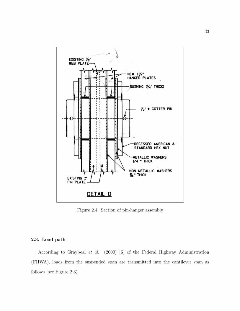
Figure 2.4. Section of pin-hanger assembly

2.3. Load path

According to Graybeal et al. (2000) [6] of the Federal Highway Administration

(FHWA), loads from the suspended span are transmitted into the cantilever span as

follows (see Figure 2.3).

34

• The loads travel from the suspended girder web to the lower pin, and then into

the hanger plates.

• From the hanger plates, the loads are transferred into the upper pin, and finally

into the cantilevered girder web.

These connections are designed to support the transfer of shear forces from the sus-

pended span into the cantilever span.

Shear planes

Pin

Hanger plates

plateWeb

Figure 2.5. Shear planes of the connection

The load path, mentioned above, creates two shear planes within each pin, as illustrated

in Figure 2.5, one at each of the intersection of the web plate and the hanger plate. If

35

a pin fails along shear planes, the portion of the bridge section suspended by that pin

would be unsupported.

The inclusion of hinges (Figure 2.2), as back up joint assemblies, will help as an

alternative load paths and redundancy. This means that if a pin-and-hanger assembly

failed, the assembly (hinge connection) could provide an alternative load path.

2.4. “Pack rust” formation

The joint assemblies are in general located directly beneath bridge deck expansion

joints. Consequently, they are often exposed to water and debris that falls through the

joints. Water and debris can accumulate behind the hanger plate and around the pins.

Moreover, the presence of moisture in the confined region between the hanger plates and

girder web can lead to an expansion or packing of rust flakes caused by corrosion, also

called “pack rust”. Furthermore, due to gravity, as depicted in Figure 2.6, moistures falls

to the lower pin and it tends to lock-up first. Also, in Appendix, we present a method on

how to estimate the rate of corrosion expansion.

In most cases, the pack-rust can have two detrimental effects on the pin, [6]:

• First, the cross-section of the pin can decrease because of corrosive section loss.

In addition, the corrosion can produce pitting that may act as crack initiation

sites.

• Second, pack-rust can effectively lock the pin within the connection, so that no

rotation about the pin is permitted. This can lead to large torsional stresses,

which may produce a likely location for the development and propagation of

cracks and the eventual failure of the pin.

36

Pack rust

(bottom pin)

Hanger

Pin

PinPin

Pin

Figure 2.6. Typical pack rust formation

On the other hand, locating cracks that initiate on the pin barrel at the shear perimeter

is a difficult task. The shear plane is not visible unless the pin is removed from the

connection, as shown in Figure 2.7, (Graybeal et al., 2000 [6]). This operation is labor

and equipment intensive.

37

As shown in the previous picture (2.6), pack-rust is a thick build-up of corrosion

product that tends to develop between the surfaces of closely joined and unprotected

metal parts (unpainted joints, for example), in particular in older or aging structures.

According to our calculation (see Appendix C for details), the volume of rust produced

by corrosion is about 3.5 times that of the parent metal; i.e., full corrosion of 1/4 inch of

metal will cause about 1 inch of pack rust.

2.5. Wear grooves

As indicated by Graybeal et al. (2000) [6], the combined results of the ultrasonic

testing and visual examination revealed shallow defects in some of the pins and no defects

in the hanger links. In general, these shallow defects were reported as wear grooves or

corrosion section loss having depth ranging from minimal to 3mm (1/8in.). Pins with

wear grooves on the surfaces are illustrated in Figure 2.7.

38

Shear planes

(wear grooves)

Figure 2.7. Shallow defects or wear grooves (Removed pins)

39

CHAPTER 3

Finite element modeling

3.1. Geometry and model

A schematic representation of the intermediate span elevation is illustrated in Figure

3.1.

CLHINGE PIN−HANGER

CL OF

CANTILEVEREDSPAN

P = 268 kips (1192 kN)

CANTILEVERED

61 ft (18.6 m)61 ft (18.6 m) 122 ft (37.2 m)

244 ft (74.4 m)

SPAN

CL OF

SUSPENDEDSPAN

Figure 3.1. Schematic representation of the intermediate span elevation

With a reasonable approximation, the symmetry of the model is taken in the middle

of the intermediate span. With this as a boundary condition, only the right half of the

structure (which contains pin-hanger assembly) needs to be considered. In addition, due

to the pier support, the boundary condition on the right pier (cantilever span) is taken

to be a built-in support. Finally, the third boundary condition is taken in the z-direction

(1/2 web girder). Since the model is symmetric with respect to x − y plane and y − z

plane, only 1/4 of it needs to be discretized.

40

Detailed simulations of the bridge structure, which consists of a suspended span, a

cantilever span, and a complete set of elements of the joint connection, were carried out

with the ABAQUS finite element program [2].

The finite element mesh of the bridge model is shown in Figure 3.2.

3.1.1. Model validation

Since analytical solution are not available in many cases, especially for this 3D problem

with complex geometry and loading conditions, a series of model validation tests are

performed:

• Check tension versus applied load

• Verify stress concentration near the hole

• Validate tension versus design calculation

The corresponding results will be shown later in this Chapter.

3.1.2. Geometric dimensions

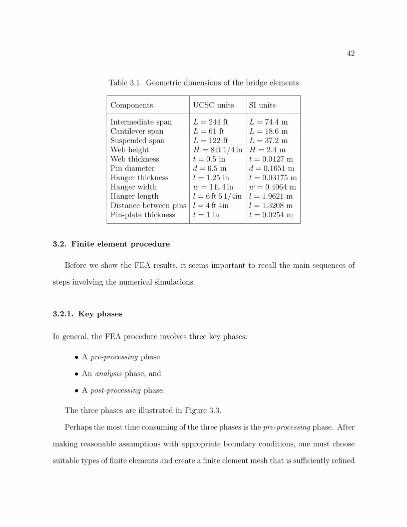
The geometric dimensions of the bridge elements are summarized in Table 3.1. The units

of dimension and force are consistent. Every data in this report are given in both, the

United States Customary System (USCS) and the Systeme International d’Unites (SI).

The USCS is generally given first, followed by the SI value in parentheses. Thus, if the

USCS unit is 61 ft, it will be expressed as 61 ft (18.6 m).

Note that all dimensions are given in meters (SI units) for the computations. Conse-

quently, the outputs are automatically displayed with SI units. For convenience, we will

convert, if necessary, the solution data from SI units to USCS units.

41

X

Y

Z

Sus

pend

ed S

pan

Can

tilev

erd

Spa

n

Join

t Con

nect

ion

Figure 3.2. Finite element model of the bridge

42

Table 3.1. Geometric dimensions of the bridge elements

Components UCSC units SI units

Intermediate span L = 244 ft L = 74.4 mCantilever span L = 61 ft L = 18.6 mSuspended span L = 122 ft L = 37.2 mWeb height H = 8 ft 1/4 in H = 2.4 mWeb thickness t = 0.5 in t = 0.0127 mPin diameter d = 6.5 in d = 0.1651 mHanger thickness t = 1.25 in t = 0.03175 mHanger width w = 1 ft 4 in w = 0.4064 mHanger length l = 6 ft 5 1/4in l = 1.9621 mDistance between pins l = 4 ft 4in l = 1.3208 mPin-plate thickness t = 1 in t = 0.0254 m

3.2. Finite element procedure

Before we show the FEA results, it seems important to recall the main sequences of

steps involving the numerical simulations.

3.2.1. Key phases

In general, the FEA procedure involves three key phases:

• A pre-processing phase

• An analysis phase, and

• A post-processing phase.

The three phases are illustrated in Figure 3.3.

Perhaps the most time consuming of the three phases is the pre-processing phase. After

making reasonable assumptions with appropriate boundary conditions, one must choose

suitable types of finite elements and create a finite element mesh that is sufficiently refined

43

Output files

Simulation

Input file

Postrocessing ABAQUS/CAE or other software

ABAQUS/CAE or other softwarePreprocessing

Figure 3.3. Different stages of analysis

in regions where high stress distribution is expected; i.e. the connection areas between

joint components.

For the most part, the analysis phase is straightforward. However, in the final phase,

one faces the difficult task of interpreting the results of the analysis. The post-processing

phase has been made easier through post-processing software. In addition, at this stage,

one must assess whether or not the “nice-looking” contour plots make sense. In particular,

one must be able to answer questions such as: Are the boundary conditions satisfied? Is

the finite element mesh sufficiently refined? Is the assumption of linear material behavior

44

appropriate? Are the applied loads accurate? etc. Other sources of information include

Cook et al. (2002) [8], Gosz (2006) [9], and ABAQUS (2003) [2].

3.2.2. Mesh generation

As mentioned above, mesh generation by itself is a time consuming process. With the

arrival of modern pre-processing software, the amount of time spent in the pre-processing

phase has been significantly reduced.

For example, the geometric model of each component covered by this study necessitates

the use of an automatic mesh generator (pre-processing program). This must be capable

of producing fine elements near the assemblies where the stress gradients are changing very

rapidly, and coarser elements in regions where the stresses are more evenly distributed.

The elements should not be excessively elongated or distorted, [2].

3.2.3. ABAQUS/CAE

ABAQUS/CAE provides a complete modeling (pre-processing) and visualization environ-

ment (post-processing) for ABAQUS analysis products. Here, CAE stands for “Complete

ABAQUS Environment”, not to be confused with “Computer Assisted Engineering”, a

term commonly employed in the field of design and simulation. The ABAQUS suite con-

sists of three core products: ABAQUS/CAE, ABAQUS/Standard, and ABAQUS/Explicit.

ABAQUS/CAE provides a consistent interface for creating finite element model for

ABAQUS solver (Standard or Explicit). It produces a data file (called model database)

for immediate analysis by the solver. For example, ABAQUS/CAE has been used here

to build a complete bridge model.

45

ABAQUS/CAE is divided into modules, where each module defines a logical aspect of

the modeling process. For example, defining the geometry, defining material properties,

and generating a mesh. As we move from module to module, we build the model from

which ABAQUS/CAE generates an input file that we then submit to the solver. Finally,

we use the visualization module to view the results of our analysis.

Here, the bridge model is organized as a collection of individual parts, also called

instances, connected together to form a one piece of structure. We then position those

instances relative to each other in a global coordinate system to form the assembly. We can

create and position multiple instances of a single part; e.g. we can create multiple instances

of a single part of pin (upper and lower pins). In addition, we can assemble instances of

deformable parts; e.g. hanger, webs, pins, when we are solving contact problems. When

we modify a part, ABAQUS/CAE automatically regenerates all instances of the modified

part in the assembly.

For further details, one can refer to ABAQUS documentation (2003) [2].

3.3. Finite element analysis (FEA)

3.3.1. Model discretization

All structural components (web girders, pins, hanger, and reinforcement plates) are

modeled 8-node standard brick reduced-integration elements (known as C3D8R in the

ABAQUS element library). The entire model consists of about 31,000 elements. The

density of the mesh increases toward the centers of the connections where most of the

deformation occurs.

46

Since the problem involves contact interactions between different components, also

known as 3D multi-body contacts, first order brick elements are the best choice for this

type of problem. In addition, reduced-integration elements are used, because among

other considerations, it decreases the analysis cost, and provides reasonable accuracy on

stress prediction, [2]. Figure 3.4 illustrates typical brick elements: linear and quadratic

elements.

(a) Linear element (8−node brick)

(b) Quadratic element (20−node brick)

Figure 3.4. Linear and quadratic brick elements

Figure 3.5 shows the discretization in the vicinity of the joint connection which is the

region of interest. Note that the mesh is finer toward the vicinity of the contact surfaces

where the stresses are highest.

3.3.2. Material properties

We assume that the entire bridge is made of the same construction material (ASTM A36).

A Young’s modulus of E = 29× 106 psi (200 GPa) and a Poisson’s ratio of ν = 0.3 define

the elastic response of the material. The initial yield stress is σY = 36 ksi (248 MPa)

47

X

Y

Z

Han

ger

Pin Pin

Figure 3.5. Finite element mesh in vicinity of pin-hanger connection

48

and the ultimate tensile strength of σUTS = 58 ksi (400 MPa). The coefficient of thermal

expansion is α = 6.5× 10−6/ F (α = 11.7× 10−6/ C). These values are recapitulated in

Table 3.2.

Table 3.2. Material properties (ASTM A36)

MaterialσY σUTS α (×10−6)

ksi MPa ksi MPa /F /C

ASTM A36 36 248 58 400 6.5 11.7

3.3.3. Loading

3.3.3.1. Mechanical loading. According to the document provided by the Wisconsin

Department of Transportation (WisDOT) (1999) [10], it was estimated that the total

load for one girder, which includes dead load, traffic and impact, is equal to 268, 000 lbf

(121, 563 kgf).

P = DL + (LL + I)

= 197, 000 lbf + 71, 000 lbf

= 268, 000 lbf

= 268 kips

where DL, LL, I are dead load, live load, and impact respectively. Therefore,

DL = 197 kips

LL + I = 71 kips

49

In this model, the dead load is approximately 3 times the live load and impact. Note that

the design calculations can be found in Appendix A.

As a result, an analysis of the bridge under the design external load of 268 kips (1192

kN) was carried out. The load was applied at the top of the suspended web girder at the

pin-hanger connection, which is known as the critical location for the bridge structure.

We recall here the load path described in the previous Chapter. As a result, we apply the

same load path for the FEA computations.

3.3.3.2. Thermal load. A new and simple method is proposed to evaluate the bridge

movements due to temperature changes. We present an analytical expression and the

comparison with the corresponding finite element solution. We will discuss this in detail

in Chapter 5.

3.3.4. Contact modeling

The contact analysis was performed using the contact pair approach in ABAQUS. Contact

pairs, named as master and slave surfaces define surfaces which can potentially come into

contact. In the present study, the contact is modeled by the interaction of contact surfaces

defined by grouping specific faces of the elements in the contacting regions. Here, surface-

to-surface contact is defined between:

• the suspended web-girder and the lower-pin,

• the lower-pin and the bottom-hole of the hanger plate,

• the top-hole of the hanger plate and the upper-pin, and

• the upper-pin and the cantilever span.

Thus, 4 multi-body contacts were defined to describe the deformable surfaces in 3D.

50

Normal pressure will be transmitted through the contact pairs. In ABAQUS, contact

can occur in the form of small sliding or finite sliding. Analyses performed in this work

used the small sliding option, in which surfaces are allowed to undergo finite separation and

sliding. Contact surface tractions were calculated assuming that the surfaces are perfectly

hard, which means that there will be no penetration of surfaces into one another. Contact

tractions were defined by local basis system formed by the normal to the master surface.

To perform the first series of simulations (stress analysis), a coefficient of friction

µ = 0 is used between all contacting surfaces which correspond to the unlocked (unfrozen)

condition.

In addition, the analyses were performed using small-displacement theory. The only

nonlinearities in the problem are the result of changing conditions due to contact inter-

actions.

3.3.5. Results

We investigate here several different approaches to simulate the pin and hanger connec-

tions. In addition, the analysis is first performed by assuming a linear elastic material

behavior and frictionless contacts, i.e. unlocking scenario. This simple material model

would probably suffice for routine design.

We have mentioned before the need for the validation of our finite element model. This

is mainly due to the complexity of the geometry and boundary conditions. Therefore, a

series of validation tests were performed. These include:

• Check the tension in the hanger plate if there is consistency between the applied

mechanical load and the corresponding tension in the hanger plate.

51

• Compare the results between the design calculation and the finite element analysis

prediction (near the connection).

• Check the stress concentration in the hanger plate.

3.3.5.1. Checking tension in the hanger against applied load. First, we check the

tension in the hanger versus the applied load (Figure 3.6). Axial loading is a load passing

through the body of the hanger plate. This is the type of load when the plate is designed.

We assume that there is no friction between components in the joint assemblies. Based

on that assumption, we should obtain the same amount of applied load and tension (or

axial stress) in the hanger plate. Note that the axial stress S22 (or σ22), as depicted in

(Avg: 75%)S, S22

−1.108e+08−8.867e+07−6.657e+07−4.447e+07−2.238e+07−2.764e+05+2.182e+07+4.392e+07+6.602e+07+8.812e+07+1.102e+08+1.323e+08+1.544e+08

X

Y

Z

Tension predictionvs applied load

Figure 3.6. Contour axial stress (S22)

52

Figure 3.6, is expressed in Pascals (SI units). In order to convert to kilopound per square

inch (kips), we need to perform the following steps.

According to the FEA prediction, as depicted in Figure 3.7, the averaged axial

stress σ22 (or S22) is:

σ22 = 46.2× 106 Pa

= 6.70 ksi

The cross sectional area (A) of the hanger plate is

A = 16 in× 1.25 in

= 20 in2

Therefore, the tension in the hanger is

t = σ22 × A

= 6.70× 20

= 134 kips

Note that the applied load was P = 134 kips. Here, the result of our computation

for the tension in hanger is t = 134 kips. Therefore, an excellent agreement was

obtained. Consequently, the first model validation is checked.

It is clear, by the results presented, that our FEA model with current boundary conditions

and 8-node brick elements (with reduced-integration) provide sufficient accuracy.

53

Hanger width, [normalized]0.0 0.2 0.4 0.6 0.8 1.0

Axi

al S

tres

s S

22, [

Pa]

44.0

44.4

44.8

45.2

45.6

46.0

46.4

46.8

47.2

47.6

48.0

48.4[x1.E6]

Figure 3.7. Plot of the tension in the middle of the hanger plate

3.3.5.2. Comparing design calculations against FEA predictions. Because stress

concentrations occur at the hanger holes, the net section of the hanger plate across the

hanger hole is the critical section for carrying load. The solutions are summarized in

Table 3.3. It shows the results which compare the design calculations, the corresponding

data provided by the American Association of State Highway and Transportation Officials

specification, AASHTO (1996) [11], and the finite element analysis (FEA) solutions.

Table 3.3. Comparison of the tension in hanger near the pin hole

StressDESIGN AASHTO FEA

ksi MPa ksi MPa ksi MPa

Tension in Hanger 12.43 85.70 27.72 191.12 11.63 80.20

54

As the results show, an excellent agreement is found between the design calculations

(12.43 ksi) and the FEA prediction (11.63 ksi). The design data is slightly more conserva-

tive. The relative error is less than 7%. The FEA data (11.63 ksi) were obtained by taking

the average of the tension near the hanger hole (Figure 3.8). Accordingly, we found that

both design calculations and finite element solutions are far below the maximum allowable

stresses (27.70 ksi) dictated by the AASHTO recommendations.

Hanger Width, [normalized]0.0 0.2 0.4 0.6 0.8 1.0

Axi

al S

tres

s S

22, [

Pa]

0.04

0.06

0.08

0.10

0.12

0.14

0.16[x1.E9]

Figure 3.8. Tension near the hanger hole

3.3.5.3. Stress concentration in hanger plate. Consider the circular hole (on top of

the hanger plate), as illustrated in Figure 3.9, it is known that the local tangential stress

at the edge of the hole is at least three times the applied far-field stress. Here, we found

that the stress concentration near the hole is 3.27 times higher than the far-field axial

55

stress (see Figures 3.10 and 3.9). Therefore, the FEA results confirm the accuracy of

the computations when compared with analytical solution (a stress concentration greater

than 3.0 is to be expected because of the effect of the pin in the hole).

In addition, Figure 3.10 shows the axial stress profile across the section of the hanger

width. As indicated by this profile, the magnitude of this localized stress diminishes with

distance away from the hole.

End: 420181218171816181518141813451542203620372038203920402035Start: 511

X

Y

Z

Figure 3.9. Stress concentration prediction

3.3.5.4. Shear stress in the pin. There is another verification recommended by AASHTO,

which is to verify the maximum allowable shear stress in the pin. Table 3.4 summarizes the

results by comparing shear stress values. We found that the design calculation (average

56

Half−distance of the hanger width, [normalized]0.0 0.2 0.4 0.6 0.8 1.0

Str

ess

prof

ile a

long

the

hang

er w

idth

, [P

a]

0.06

0.08

0.10

0.12

0.14

[x1.E9]

Figure 3.10. Axial stress profile across the hanger cross section

shear) and finite element prediction (maximum shear) are below the maximum allowable

stress dictated by the AASHTO recommendations.

Table 3.4. Shear stress in the pin

StressDESIGN AASHTO FEA

ksi MPa ksi MPa ksi MPa

Shear in Pin 4.04 27.85 14.40 99.28 8.37 57.73

3.3.5.5. von Mises equivalent stress distribution. Table 3.5 recapitulates the FEA

results of the von Mises equivalent stresses (σeq) in each component of the assembly. These

values are then compared to the yield stress, σY , of the materials (ASTM A36). Stress

levels in the pin and hanger are below yield, as expected.

57

(Avg

: 75%

)S

, Mis

es +1.

437e

+04

+2.

493e

+07

+4.

984e

+07

+7.

476e

+07

+9.

967e

+07

+1.

246e

+08

+1.

495e

+08

+1.

744e

+08

+1.

993e

+08

+2.

242e

+08

+2.

492e

+08

+2.

741e

+08

+2.

990e

+08

X

Y

Z

Hig

h st

ress

dis

trib

utio

n in

the

cant

ileve

r sp

an

Figure 3.11. von Mises equivalent stress distribution

58

(Avg

: 75%

)S

, Mis

es +1.

437e

+04

+2.

493e

+07

+4.

984e

+07

+7.

476e

+07

+9.

967e

+07

+1.

246e

+08

+1.

495e

+08

+1.

744e

+08

+1.

993e

+08

+2.

242e

+08

+2.

492e

+08

+2.

741e

+08

+2.

990e

+08

X

Y

Z

Hig

h st

ress

con

cent

ratio

n in

bot

h jo

int c

onne

ctio

ns

Figure 3.12. von Mises equivalent stress near joint connection

59

Table 3.5. von Mises equivalent stress σeq in bridge components

Components σeq σeq/σY

Pin (bottom) 32.88 ksi 0.91Pin (top) 32.79 ksi 0.91Hanger 22.91 ksi 0.64

3.4. Concluding remarks

The results of the design calculations and the finite element analyses are seen to agree

closely. The results also suggest that our 3D finite element model is a suitable model for

the bridge problem. Furthermore, the accurate results we obtain confirm that the model

is properly constrained and the choice of element as well as the selection of the contact

algorithm is satisfactory. There is another issue that may affect the results as well, which

is the contact interaction. It is important to note that if the contact procedure is not

taken into account properly, the final results of the computation are greatly affected and

can be completely wrong. This topic is not straightforward from the engineering point of

view.

Additional sources of information include Belytschko et al. (2000) [12], Wriggers

(2002) [13], and ABAQUS theory manual (2003) [2], amongst others.

It should be noted that the von Mises stress is an “equivalent” stress which is the result

of the conversion from a multiaxial state of stress to an equivalent state of stress. Note

that the resulting stress field is fully tree-dimensional. Therefore, the yielding condition is

obtained by converting 3D states of stress to equivalent 1D states which can be used with

uniaxial experimental data (i.e., yield strength of the material used). As a result, this

60

equivalence is not perfect. Also, the von Mises equivalent stress (σeq) is always positive

and does not identify the algebraic signs of stresses that contribute to it.

61

CHAPTER 4

Constitutive equations

4.1. Introduction

The aim of this Chapter is to set up constitutive equations required to describe the

physical stress-strain response of the bridge subjected to applied loads. The mechanical

constitutive models often consider elastic and inelastic response. The inelastic response

is most commonly created with plasticity models.

In the previous Chapter, the finite element modeling of the bridge was entirely based

on an elastic response of the structure. For example, a mechanical component; i.e. hanger

plate, made from a standard structural steel (ASTM A36), can be modeled as an isotropic

and linear elastic material. This simple material model would probably suffice for rou-

tine design, so long as the component is not in any critical situation. However, if the

component might be subjected to a severe overload, it is important to determine how it

might deform under that load and if it has sufficient ductility to withstand the overload

without catastrophic failure. In that case, the elastic-plastic material model will also be

considered.

It is important to note that most engineering materials have a linear elastic behavior

at the early stages of deformations. However, when certain criteria are reached; e.g., yield

condition, several materials undergo permanent or plastic deformation.

62

4.2. Elasticity

As mentioned above, we first consider the simplest of these models, the linear elastic

material model. Hooke’s law for linearly elastic materials states that there is a linear

relationship between the Cauchy stress and the small strain. The relationship between

stress and strain can be written as,

(4.1) σ = C : εel

where σ denotes the Cauchy stress tensor, εel is the elastic strain tensor, and C (often

denoted by D in some literature) is the fourth-order elasticity tensor.

For further details, one can refer to Timoshenko (1951) [14] and Malvern (1969) [15],

amongst others, for references to the literature.

It is somehow interesting to note that the tensor notation, i.e. Eq. 4.1, is very elegant

when it comes to theoretical derivations. The tensor notation is appealing because it al-

lows the equations to be developed concisely without the complexities with the component

form (also called index notation) in a particular basis system. However, for the purpose

of applications, it is often more practical to work with the component form. Accordingly,

Eq. 4.1 can be rewritten as,

(4.2) σij = Cijkl εelkl

63

Note that indices i, j, k, and l take on values 1, . . . , n, where n is the spatial dimensions,

and the summation convention applies to repeated indices i, j, k, and l.

For an isotropic material, C takes a form ensuring that the material has the same

properties in every direction. An isotropic fourth-order tensor C has the form,

(4.3) Cijkl = λδijδkl + µ(δikδjl + δilδjk)

where λ and µ are Lame constants. After substituting Eq. 4.3 into Eq. 4.2, we obtain,

(4.4) σij = (λδijδkl + 2µδikδjl) εelkl

where δij, . . . , δjk denote Kronecker deltas. The Kronecker delta is defined as,

δij =

1 if i = j

0 if i 6= j

Therefore, the stress components becomes,

(4.5) σij = λεkkδij + 2µεij

In tensor notation, Eq. 4.5 can be written as,

(4.6) σ = λ trace(ε)I + 2µε

where trace(ε) = εkk, the sum of the diagonal elements, and I is the identity matrix.

64

In engineering practice, it is common to use engineering constants instead of the Lame

constants. The engineering constants are Young’s modulus (E), Poisson’s ratio (ν), and

shear modulus (G). Thus, the relationships between these constants are,

(4.7) λ =νE

(1 + ν)(1− 2ν), µ = G =

E

2(1 + ν)

After substituting these constants in Eq. 4.5, we obtain,

(4.8) σij =νE

(1 + ν)(1− 2ν)εkk δij +

E

1 + νεij

In tensor notation, Eq. 4.8 becomes

(4.9) σ =νE

(1 + ν)(1− 2ν)(trace (ε))I +

E

1 + νε

Writing explicitly stress and elastic strain in column vectors, Hooke’s law, in a three-

dimensional state of stress, becomes

(4.10)

σxx

σyy

σzz

σxy

σyz

σzx

=

E(1− ν) Eν Eν 0 0 0

Eν E(1− ν) Eν 0 0 0

Eν Eν E(1− ν) 0 0 0

0 0 0 G 0 0

0 0 0 0 G 0

0 0 0 0 0 G

εxx

εyy

εzz

γxy

γyz

γzx

65

where,

E =E

(1 + ν)(1− 2ν)

and,

γxy = 2εxy

γyz = 2εyz

γxz = 2εxz

where γ is used to represent engineering shear strain because of its convenient geometric

interpretation.

For further details, one can refer to Timoshenko (1951) [14], Fung (1965) [16], and

Malvern (1969) [15], amongst others, for references to the literature.

4.3. Equilibrium equation

Let us consider an equilibrium problem in linear elasticity for an isotropic material.

The problem consists of determining the displacements, strains, and stresses that satisfy

the partial differential equations of equilibrium,

(4.11)∂σij

∂xj

+ bi = 0

Using component form, Eq. 4.11 can be rewritten as,

(4.12) σij,j + bi = 0

where bi defines the body force.

66

From the previous Section, the constitutive relation has been defined as,

(4.13) σij = λεkkδij + 2µεij

And the strain and displacement relation can be written using component form as follows,

(4.14) εij =1

2(ui,j + uj,i)

Further details can be found in Timoshenko (1951) [14], Malvern (1969) [15], Be-

lytschko et al. (2000) [12], Holzapfel (2000) [17], and ABAQUS Theory Manual (2003)

[2].

4.4. Thermal strain

The temperature field dictates the thermal strain distribution in the solid, which in

turn gives rise to thermal stresses when the solid is constrained. In other words, the

thermal strain loads the solid. When a solid body is heated, the body expands. Likewise,

when a solid body is cooled, it contracts. If thermal strains is included, then,

(4.15) ε = εel + εth

where εth is the thermal strain and εel the elastic strain.

For an isotropic material,

(4.16) εth = α(T − T0) I

67

in which, α is the coefficient of thermal expansion, T and T0 are current and initial

temperatures respectively, and I is the unit tensor. Using index notation, we obtain,

(4.17) εthij = α∆Tδij

where ∆T denotes the temperature change.

Therefore, Hooke’s law for thermoelastic problems can be written as,

(4.18) σij = Cijkl(εkl − α∆Tδkl)

4.5. Elasto-plastic material behavior

4.5.1. Basic concepts

As the external loads (mechanical, thermal, environmental) acting on the structure are

gradually increased, plastic deformation may take place. This means that, upon removal

of the external loads, the elements of the structure do not return to their original shapes.

Under such conditions, the stress-strain response of the material is nonlinear, even in the

small strain regime. Most engineering materials have a linear elastic behavior at the early

stages of deformations. However, when certain criteria are reached (e.g., yield condition),

several materials undergo permanent or plastic deformation.

Under small-strain condition, we can decompose the total strain (ε) into elastic (εel)

and plastic (εpl) parts as follows,

(4.19) ε = εel + εpl

68

and in rate form,

(4.20) ε = εel + εpl

Then the isotropic elastic constitutive equation may be written as,

(4.21) σ = λ trace(εel) I + 2µ εel

When the material is flowing inelastically, the inelastic part of the deformation is

defined by the flow rule, which we can write as,

(4.22) εpl = λ Γij

where,

(4.23) Γij =3

2σSij

here, Sij is the deviatoric stress. The deviatoric stress components, Sij, are obtained by

subtracting the mean stress from the Cauchy stress components as follows,

(4.24) Sij = σij − 1

3σkk δij

and σ is defined as,

(4.25) σ =

√3

2SijSij

69

Similarly, the total accumulated plastic strain, εpl, can be expressed as,

(4.26) εpl =

∫ εplij

0

d εpl =

∫ εplij

0

˙εpl dt

where,

(4.27) ˙εpl =

√2

3εpl

ij εplij

Other sources of information include Hill (1950) [18], Owen and Hinton (1980) [19],

Crisfied (1991) [20], Khan et al. (1995) [21], and ABAQUS Theory Manual (2003) [2].

4.5.2. Yield condition

The yield condition is in general referred to as a yield function or yield surface. A

important yield condition for ductile metals is the von Mises yield condition developed

by Richard von Mises (1913). The von Mises yield condition ignores the third invariant

of the deviatoric stress tensor and assumes that the yield function only depends on J2.

This condition can be written as,

(4.28) J2 − k2 = 0

where k is a scalar quantity.

70

When the yield condition is assumed to be isotropic, a general state of stress at a

point can be written in terms of the principal stress as,

(4.29)

σ1 0 0

0 σ2 0

0 0 σ3

As mentioned previously, the deviatoric part of the stress (Eq. 4.29) is obtained as

follows,

(4.30) S = pI + σ

where S is the deviatoric part of the Cauchy stress tensor σ;

(4.31) p = −1

3σ : I

where p is the hydrostatic pressure and I is the second-order identity tensor.

Thus, Eq. 4.30 becomes

S = pI + σ

=

2σ1 − σ2 − σ3 0 0

0 2σ2 − σ1 − σ3 0

0 0 2σ3 − σ1 − σ2

(4.32)

The quantity J2 turns out to be

(4.33) J2 =1

3(σ2

1 + σ22 + σ2

3 − σ1σ2 − σ1σ3 − σ2σ3)

71

The von Mises yield condition can be written in terms of the 3 principal stresses as,

(4.34) (σ21 + σ2

2 + σ23 − σ1σ2 − σ1σ3 − σ2σ3) + 3k2

The von Mises equivalent stress, σeq, is defined as

(4.35) σeq =√

3J2

and the von Mises yield condition is written as,

(4.36) σeq −√

3k = 0

The yield condition in this form is convenient to use in practice. One can assess whether

a component can be expected to yield under external loadings by performing a linear

finite element analysis and then observing a contour plot of the von Mises equivalent

stress (σeq). If σeq ≥ σY at a particular location, then the component can be expected to

yield at that location. Here, σY defines the yield stress of the materials. Details of the

calculations which refer to the von Mises yield condition can be found in Chapter 3.

4.6. Contact modeling

The objective of this section is to describe the contact interaction between different

part components which form the joint assemblies; i.e. web girder and pin, pin and hanger,

etc. Also, the bridge components in contact to each other are assumed to be deformable

bodies.

The contact problem which involves 3D multi-body interaction is probably the most

challenging issue in numerical modeling. If contact procedures are not taken into account

72

properly, the final results of the computation are greatly affected and can be completely

wrong. The topic is not straightforward from the engineering point of view.

Furthermore, in the current project, we intend to use the friction capability to simulate

the “frozen” and “unfrozen” conditions, also called “locking” and “unlocking” conditions,

between the pin and the hanger.

4.6.1. Basic concepts

In finite element analysis, contact conditions are a special class of discontinuous constraint,

allowing forces to be transmitted from one part of the model to another.

The constraint is discontinuous because it is applied only when the surfaces are in

contact. When the surfaces separate, no constraint is applied. Therefore, the analysis has

to be able to detect when two surfaces are in contact and apply the contact constraint

accordingly. Similarly, the analysis must be able to detect when two surfaces separate

and remove the contact constraints.

Other sources of information regarding this topic can be found in Belytschko et al.

(2000) [12], Wriggers (2002) [13], and ABAQUS Theory Manual (2003) [2].

4.6.2. Contact capabilities in ABAQUS

ABAQUS provides two algorithms for modeling the interaction between deformable bod-

ies.

The first algorithm is called a small-sliding formulation in which the contacting sur-

faces can undergo only small sliding relative to each other, but arbitrary rotation of the

73

surfaces is permitted. The second algorithm is called a finite-sliding formulation where

separation and sliding of finite amplitude may arise.

Among other considerations, small-sliding contact is computationally less expensive

than finite-sliding contact.

Contact simulations in ABAQUS are surface based contact. Surfaces that will be

involved in contact must be created on the various components in the model; i.e. pin,

hanger, web-girder. Then, the pairs of surfaces that may contact each other known as

contact pairs, must be identified. Finally, the constitutive model governing the interaction

between the various surfaces must be defined.

With this approach, one surface definition provides “master” surface and the other

surface definition provides “slave” surface. In addition, a kinematic constraint that the

slave surface nodes do not penetrate the master surface is then enforced ([2]).

4.6.3. Friction

The Coulomb friction model is used with all contact analyses. It states that the critical

stress, τcr, is proportional to the contact pressure, p, in the form

(4.37) τcr = µ p

An extended version of the classical isotropic Coulomb friction model is provided in

ABAQUS. The extensions mainly include an additional limit on the allowable shear stress.

The Coulomb friction model assumes that no relative motion occurs if the equivalent

74

frictional stress, τeq, is less than the critical stress, τcrit, ([2]).

(4.38) τeq < τcrit

in which, τeq and τcrit are defined as follows,

τeq =√

τ 21 + τ 2

2

and,

τcrit = µ p

where µ is the friction coefficient that can be defined as a function of contact pressure

(p), slip rate (γeq), the surface temperature, and the field variables at the contact point.

τ1 and τ2 denote shear stresses in the tangential directions t1 and t2.

In practice, the problem usually reduces to knowing a friction coefficient under oper-

ating conditions.

A special case of friction is called “rough” friction. The rough friction parameter was

used in the definition of the contact surfaces. This implies that when the pin, the hanger,

and web girder come into contact, no relative slipping is allowed. Here, rough friction is

used to simulate the frozen condition, mentioned above.

75

CHAPTER 5

Thermal effects on bridge movements

5.1. Introduction

Our primary objective here is to develop a method to evaluate the bridge movements

induced due to temperature changes. The effects of thermal “forces” (due to temperature

changes) on a bridge structure are significant and should not be underestimated. These

movements have considerable impact on its design and performance.

All of the bridge structural components that we have considered so far were assumed

to remain at the same temperature while they were being loaded. Such assumption is

not realistic. In fact, bridges expand and contract due to temperature changes (daily and

seasonal changes). In general, thermal forces are caused by fluctuations in temperature

(i.e., from cold to hot or from hot to cold). The structural response under thermal

loading can be very complex, even though the overall strain is predominantly pure thermal

expansion or contraction.

As mentioned earlier, the primary function of a pin-and-hanger connection is to allow

for longitudinal thermal expansion and contraction in the bridge superstructure.

5.2. AASHTO recommendations and alternative approaches

According to Roeder (2003) [22], the temperatures used for determination of thermal

design movements in the present AASHTO specifications (AASHTO 1996, 1998) have

76

been used since 1920s. The design temperatures recommended in the AASHTO specifi-

cations sometimes predict movements that are larger or smaller than needed.

For example, the Illinois Department of Transportation (IDOT) (1992) [4] attempted

to measure the displacements of the bridge components due to temperature changes by

using a series of experimental tests. Several methods for detecting pin-hanger movements

were developed which range from simple to sophisticated. These include: (a) paper gages,

(b) paint stripes, (c) pointers, (d) strain gages, and (e) electronic rotation sensors. They

pointed out that the results using these techniques were not promising. The drawbacks

include difficulty of detecting small movements and complications in installation and

operating.

5.3. Temperature ranges

In general, thermal forces are caused by fluctuations in temperature (i.e., from cold to

hot or from hot to cold). AASHTO (1996) [11] provides temperature variations depending

on whether the structure is in a moderate or cold climate region. For metal structures,

the values are given in the form of extreme hot and cold temperatures (see Table 5.1).

Table 5.1. AASHTO temperature ranges

From To

Moderate climate 0F 120FCold climate −30F 120F

5.4. Response to temperature variations

Variations in temperature distribution in bridge members can be described in terms

of a uniform temperature and a gradient temperature.

77

The uniform (average) temperature only causes changes in dimension of the member,

while the temperature gradient causes bending deformations. On the other hand, if

longitudinal expansion is prevented, the girder may experience large axial forces, which

could lead to damage of the joint connection, ([22]).

5.5. New proposed method

Here, we propose a new and simple method. Our approach consists of using mathemat-

ical expression for determining bridge movements due to thermal forces. This technique

can be used for design purposes or for bridge maintenance. For design calculation, it can

help to check the exact dimension and clearances between critical components based on

the ultimate temperature changes. In other words, the main design consequence of tem-

perature fluctuations is that these deformations must be accommodated. For example,

the designer needs to provide a pin-and-hanger connection with adequate displacement

and rotation capacities. The details of the method will be described in the following

sections.

5.5.1. Thermal strain

As mentioned earlier, changes in temperature produce expansion or contraction of struc-

tural materials, resulting in thermal strains and thermal stresses. In the present study, we

assume that the temperature profile is linear and uniformly distributed over the height of

the bridge.

78

For most structural materials such as bridge structure, thermal strain, εth, is propor-

tional to the temperature change ∆T ; that is,

(5.1) εth = α(∆T )

in which α is a property of material called the coefficient of thermal expansion (CTE).

∆T is the differential between the extreme design temperatures and the installation tem-

perature.

For instance, if the bridge span length is L, then the dimension will increase by the

amount of δL,

(5.2) δL = εthL = α(∆T )L

where δL is an elongation due to thermal expansion/contraction.

5.5.2. Rotational angle

On the other hand, the expression of the rotational angle, θ, of the pin-hanger connection

relative to the reference position (Figure 5.1), is given by

(5.3) tan θ =δL

l0/2

Upon rearranging, the above equation becomes:

(5.4) θ = tan−1

[2α∆TL

l0

]

79

1/2’’

CLθ

0l

Pin

Hanger

Pin

Cantilever Web

d = 6

L = 61’−0’’

Suspended Web

H = 8’−1/4’’

L = 61’−0’’

Figure 5.1. Typical pin and hanger connection

where l0 is a segment which measure the distance between top and bottom positions of the

connections. Since the angle of rotation, θ, is a small quantity, then the above equation

(5.4) can be written as,

(5.5) θ ≈ 2α∆TL

l0

We assume that the entire bridge is made of the same construction material (ASTM

A36). A Young’s modulus of E = 29× 106 psi (200 GPa) and a Poisson’s ratio of ν = 0.3

80

define the elastic response of the typical structural material. Its coefficient of thermal

expansion (CTE) is 6.5× 10−6/F (11.7× 10−6/C) (at room temperature).

5.5.3. Numerical results

A series of finite element computations were carried out. The results of the FEA are

compared with the values obtained from the above analytical expressions (see Table 5.2).

The corresponding elongations are given in Table 5.3. They are seen to be in excellent

agreement.

Table 5.2. Comparison between exact (θ)EXACT and finite element results (θ)FEA

.

∆T (θ)EXACT (θ)FEA Error

[F] [degrees] [degrees] [%]

120 0.920 0.937 1.868 0.378 0.382 1.0-4 -0.378 -0.383 1.3-30 -0.651 -0.662 0.6

.

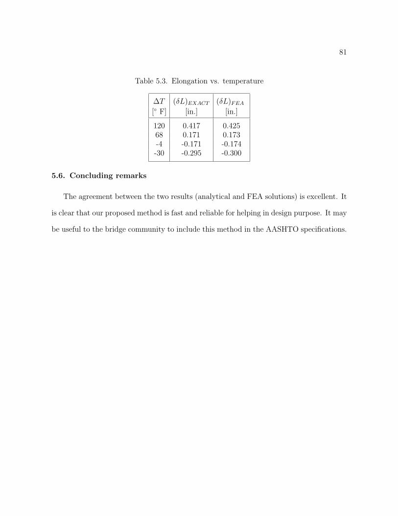
81

Table 5.3. Elongation vs. temperature

∆T (δL)EXACT (δL)FEA

[ F] [in.] [in.]

120 0.417 0.42568 0.171 0.173-4 -0.171 -0.174-30 -0.295 -0.300


The agreement between the two results (analytical and FEA solutions) is excellent. It

is clear that our proposed method is fast and reliable for helping in design purpose. It may

be useful to the bridge community to include this method in the AASHTO specifications.

82

CHAPTER 6

Operating conditions

6.1. Introduction

In this Chapter we will discuss the “operating conditions” of the bridge. This means

that we will consider two engineering aspects similar to the real-world applications of the

bridge. These include:

• lock-up condition due to pack-rust formation in the joint; and

• elastic-plastic response of the bridge structure.

6.2. Locked-up condition

As mentioned, a known problem associated with hanger plate and pin assemblies is

corrosion. The joint connection may partially or fully freeze (locked-up), thus inhibiting

the free rotation. This can lead to a large torque on the pin with plastic yielding. A

typical corrosion buildup (or pack-rust) example is shown in Figure 6.1.

According to the results (locked-up condition), as illustrated in Table 6.1, we observe

that the higher stress distribution takes place in the bottom pin with plastic yielding, and

is 1.6 times higher than in the unlocked condition. This may render the bridge unsafe for

daily use for traffic.

83

Pack rust

(bottom pin)

Hanger

Pin

PinPin

Pin

Figure 6.1. Typical pack rust formation

Table 6.1. von Mises equivalent stress σeq (locked condition)



84

6.3. Elastic-plastic behavior

All the analyses discussed so far have been considered as linear elastic. This means

that there is a linear relationship between the applied loads and the response of the

structure. In general, the bridge structure is nonlinear especially when the pin is in the

locked condition. An elastic-plastic analysis is required to model the bridge behavior

when the pin is locked.

6.3.1. Material nonlinearity

In most cases, the material behaviors fall into the following categories:

• elastic mechanical properties;

• inelastic mechanical properties;

• thermal properties; and

• general properties (density, thermal expansion, material damping).

At higher stress, metals begin to have nonlinear inelastic behavior which is referred

to as plasticity. The plastic behavior of a material is described by its yield point and its

post-yield hardening. The shift from elastic to plastic occurs at a certain point, known as

a yield point on a materials stress-strain curve.

Further details can be found in Hertzberg (1996) [23], Boresi et al. (2003) [24], and

ABAQUS User Manuals (2003) [2].

6.3.2. Defining plasticity in ABAQUS

When defining plasticity in ABAQUS, we must use true stress and true strain. However,

material test data are commonly supplied using engineering stress and engineering strain,

85

also called nominal stress and nominal strain. In such situations, we must use the ex-

pressions presented below to convert from engineering stress/strain to true stress/strain

values.

The deformation of the metal prior to reaching the yield point creates only elastic

strains, which are fully recovered if the applied load is removed. However, once the stress

in the metal exceeds the yield stress, permanent (plastic) deformation begins to occur.

The strains associated with this permanent deformation are called plastic strains. Both

elastic and plastic strains accumulate as the metal deforms in the post-yield region. The

stiffness of the metal decreases once the material yields, ([2]).

Strains in tension and compression are the same as long as ∆l → dl → 0,

dε =dl

l

thus,

ε =

∫ l

l0

dl

l

= ln

(l

l0

)

where l is the current length, l0 is the original length, and ε is the true strain or logarithmic

strain.

The true stress is defined as,

σ =F

A

where F is the force in the material and A is the current area.

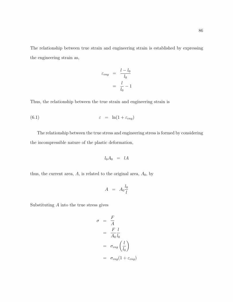
86

The relationship between true strain and engineering strain is established by expressing

the engineering strain as,

εeng =l − l0

l0

=l

l0− 1

Thus, the relationship between the true strain and engineering strain is

ε = ln(1 + εeng)(6.1)

The relationship between the true stress and engineering stress is formed by considering

the incompressible nature of the plastic deformation,

l0A0 = lA

thus, the current area, A, is related to the original area, A0, by

A = A0l0l

Substituting A into the true stress gives

σ =F

A

=F

A0

l

l0

= σeng

(l

l0

)

= σeng(1 + εeng)

87

Therefore, the relationship between true stress and engineering stress is

σ = σeng(1 + εeng)(6.2)

The plasticity model data defines the true yield stress of the material as a function of

true plastic strain.

pl el

tTrue strain

Tru

e st

ress

εε

ε

Figure 6.2. Decomposition of the total strain into elastic and plastic strains

The strains provided in material test data used to define the plastic behavior are not

likely to be the plastic strains (εpl) in the material. Instead, they will probably be the

total strains (εt) in the material. Thus, we must decompose the total strain values (εt)

88

into the elastic (εel) and plastic (εpl) components. The plastic strain (εpl) is then obtained

by subtracting the elastic strain (εel) from the total strain (εt).

This relationship is written as,

εpl = εt − εel

= εt − σ

E

where, σ is true stress and E is Young’s modulus.

6.3.3. Defining the plasticity curve

Figure 6.3 illustrates the elastic-plastic material behavior of the structural steel (ASTM

A36).

Typically, the material behavior is obtained based on simple uniaxial tests. This uni-

axial curve (stress vs. strain) is then provided to the FEA program. However, in FEA

program, the state of stress and strain is multiaxial. In order to use the uniaxial exper-

imental stress-strain curve, the FEA program “converts” the multiaxial strain tensor (6

components) in equivalent strain (1 component). This strain is called equivalent because

it converts a multiaxial state of strain to an equivalent state of strain.

Similarly, the von Mises stress is an equivalent stress which is the result of the con-

version from a multiaxial state of stress to an equivalent state of stress. Therefore, the

yielding condition is obtained by converting 3D (or 2D) states of stress and strain to

equivalent 1D states which can be used with uniaxial experimental data. As a result, this

equivalence is not perfect and depends on the plasticity theory used.

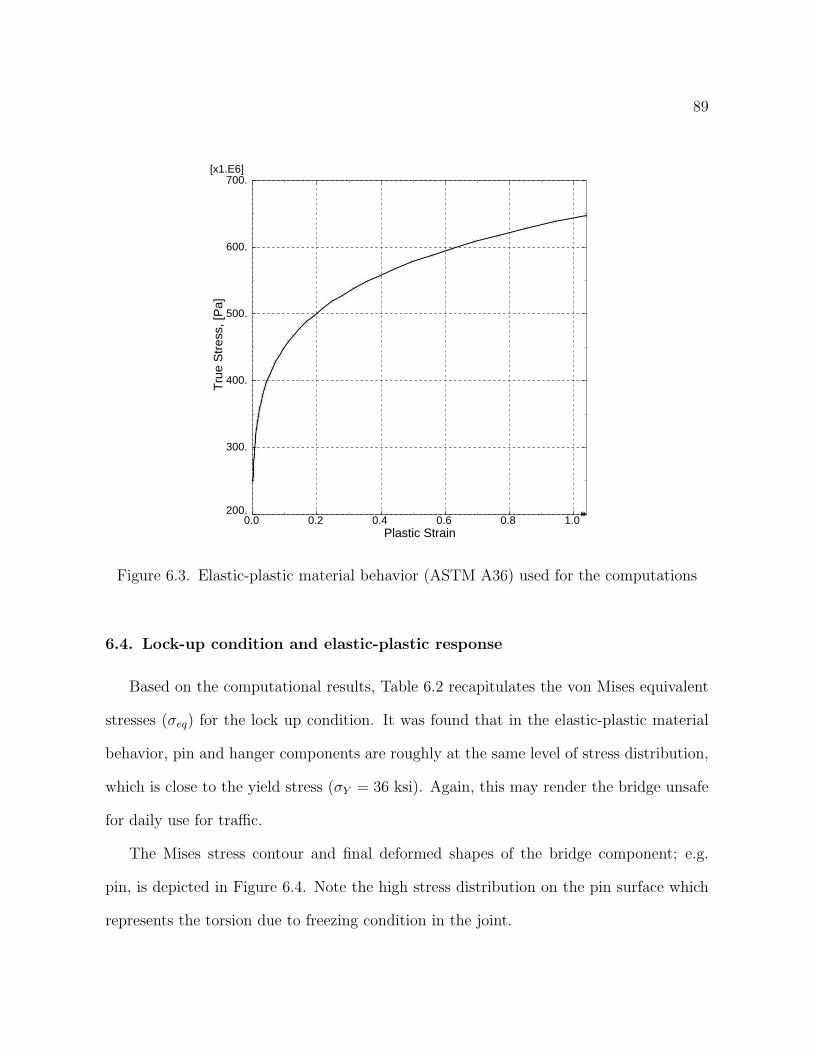
89

Plastic Strain0.0 0.2 0.4 0.6 0.8 1.0

Tru

e S

tres

s, [P

a]

200.

300.

400.

500.

600.

700.[x1.E6]

Figure 6.3. Elastic-plastic material behavior (ASTM A36) used for the computations

6.4. Lock-up condition and elastic-plastic response

Based on the computational results, Table 6.2 recapitulates the von Mises equivalent

stresses (σeq) for the lock up condition. It was found that in the elastic-plastic material

behavior, pin and hanger components are roughly at the same level of stress distribution,

which is close to the yield stress (σY = 36 ksi). Again, this may render the bridge unsafe

for daily use for traffic.

The Mises stress contour and final deformed shapes of the bridge component; e.g.

pin, is depicted in Figure 6.4. Note the high stress distribution on the pin surface which

represents the torsion due to freezing condition in the joint.

90

Table 6.2. von Mises equivalent stress σeq (locked)



(Avg: 75%)S, Mises

+3.012e+05+2.197e+07+4.364e+07+6.531e+07+8.698e+07+1.086e+08+1.303e+08+1.520e+08+1.737e+08+1.953e+08+2.170e+08+2.387e+08+2.603e+08

X

Y

Z

Figure 6.4. Mises stress on the bottom pin: lock up and elastic-plastic material

The tension prediction by FEA (in the middle of the hanger section) for the case of

full locked-up is shown in Figure 6.6 (compare with Figure 3.7 in Chapter 3). Figure 6.5

also illustrates the bending in the cross-section of the hanger. Also, note the different

profiles of the stress concentration between 2 case scenarios: lock-up and unlocked (see

Chapter 3) conditions.

91

(Avg: 75%)S, Mises

+7.838e+05+2.146e+07+4.213e+07+6.280e+07+8.347e+07+1.041e+08+1.248e+08+1.455e+08+1.662e+08+1.868e+08+2.075e+08+2.282e+08+2.488e+08

X

Y

Z

Cross−section (middle of the hanger plate)

Figure 6.5. Tension profile in the hanger plate: lock up and elastic-plastic material


We have shown the results which correspond to the so-called “operating conditions”

of the bridge. They are assumed to simulate the optimal operating conditions of the

highway bridge in extreme environmental situations:

• Freezing in the joint mechanism;

• Elastic-plastic material behavior.

The final results are slightly greater than the yield stress of the materials used (ASTM

A36). Plasticity is predicted to occur under these conditions.

92

Normalized hanger width0.00 0.20 0.40 0.60 0.80 1.00

Axi

al S

tres

s, S

22, [

Pa]

−20.

0.

20.

40.

60.

80.

100.

[x1.E6]

Figure 6.6. Axial stress in hanger for lock up and elastic-plastic material behavior

93

CHAPTER 7

Stress intensity factors for transverse crack in a pin

7.1. Introduction

The computation of the SIFs along the three-dimensional crack front remains a chal-

lenging problem. This is primarily due to the fact that accurate calculation of stress

intensity factors (SIFs) in engineering applications has been a non-trivial task.

Under repeated loadings and corrosion, cracks may develop at the surface and grow

across the section of the cylinder (pin). Small cracks developing on the cylindrical surface

have been an issue of concern over the past decades. The presence of such flaws or cracks

raises the stress and strain significantly in the vicinity of these imperfections.

Stress intensity factor solutions required to assess the structural integrity of such

configurations are lacking (Gosz and Moran, 1998 [25]). In the past, various methods,

such as the finite element method (with or without singularity elements) and the boundary

integral method, have been employed to obtain stress-intensity factor distributions for

surface cracks and corner cracks in plates (Raju and Newman, 1979 [26] and Newman

and Raju, 1983 [27]).

To address this need, another well established and useful method, known as the “do-

main integral method”, is used to obtain the mixed-mode of the stress intensity factors

(SIFs), namely mode I, mode II, and mode III. In the domain integral method, a crack-tip

contour integral is expressed as a volume integral over a finite domain surrounding the

94

crack-tip. The process of recasting the contour integral into a volume integral is advan-

tageous for numerical purposes. For a general discussion on crack-tip contour integrals

and their associated domain integral representation, see Moran and Shih, 1987 ([28] and

[29]). Contour integral evaluation is available in ABAQUS [2] for any loading (including

thermal loading) and for elastic and elastic-plastic material behaviors.

In the present study, we present the results of the evaluation of the mixed-mode stress

intensity factors (SIFs), namely KI , KII , and KIII , applied to the joint connection of

the bridge. The initial crack profile is illustrated in Figures 7.1 and 7.11. The crack

dimensions are: a = 0.236 in. (6 mm), c = 0.55 in. (14 mm), and D = 6.5 in. (165.1

mm).

X

Y

Z

Figure 7.1. Initial crack profile embedded on the pin surface

95

D

a

2c

y

x

Figure 7.2. Initial crack dimensions: a=6 mm, c=13.66 mm, D=165.1 mm

7.2. Determination of stress intensity factors

7.2.1. overview

As indicated by Schijve (2001) [30], many results of calculations on stress intensity factors

(K) for various geometries and loading cases have been published. Therefore, the first

96

approach to obtain K-values should be to consult the literature. Compilations of K-

solutions can be found in some handbooks. Frequently cited books are:

• “The Stress Analysis of Cracks Handbook”, 1973, by H. Tada, P. C. Paris, and

G. R. Irwin ([31]).

• “Stress Intensity Factors”, 1976, by D. P. Rooke and Carthwright ([32]).

• “Stress Intensity Factors Handbook”, 1987, three volumes, edited by Y. Mu-

rakami ([33]).

The above comments and suggestions are mainly concerned with plane 2D problems.

In spite of the extensive literature on K-values, it should be pointed out that in many

practical cases; i.e. the present investigation, K-solutions for cracks are not available.

Sometimes, the values can be approximated by available solutions for less complicated

geometries. Otherwise, the finite element (FE) calculations are necessary. That was the

way we proceeded for the present investigation.

The calculation techniques are significantly more complex for 3D cases with curved

crack front (as shown in Figure 7.1). There is no symmetry in this crack model. The

model validation is not always easy.

Furthermore, the three-dimensional nature of this type of crack results in the stress

intensity factors that are not only varying along the crack front, but highly sensitive to

the crack shape and the direct location of the applied load (contact pressure). As a result,

the crack shape may change as the crack grows.

Solutions derived using finite element analyses are available. Among others, Raju and

Newman (1986) [34], Shiratori et al. (1986) [35], Shih and Chen (2002) [36], and Cai

97

and Shin (2004) [37]. However, their solutions are generally limited to either only one

parameter (crack depth ratio) and one or two loading conditions (tension/bending).

In the present study, the combined loading, which results from the 3D multi-body

contact, includes compression, bending, and torsion. In the determination of fracture

parameter, such as the stress intensity factor (K), analytical solutions are needed to

check the accuracy of the numerical results. Unfortunately, there is a dearth of known

analytical solutions to 3D crack problems similar to our model. Consequently, we will

first conduct a series of tests to validate the 3D crack model. These include:

• Check the validity of a simplified 3D crack model with available results in liter-

ature (Raju and Newman, 1979 [26])

• Compute various mixed-mode problems under combined loadings using bridge

model and operating conditions.

It is interesting to note that the cylindrical-shaped components, such as pins, shafts,

and bolts, are commonly used in engineering structures. Here, we will show one approach

to solving this typical problem. First, we will introduce the basic concepts which relate

to the stress analysis of cracks and the J-integral.

7.2.2. Stress analysis of cracks

The stress intensity factors characterize the influence of load on the magnitude of the

crack-tip stress and strain fields.

To establish methods of stress analysis for cracks in elastic solids, it is convenient to

define three types of relative movements of two crack surfaces (Paris, 1965 [38]). These

98

displacement modes (Figure 7.3) represent the local deformation ahead of a crack (Barsom

and Rolfe, 1999 [39]):

• Mode I is the opening or tensile mode. The two fracture surfaces are displaced

perpendicular to each other in opposite direction.

• In Mode II, the sliding or in-plane shearing mode, the crack faces slide relative

to each others.

• In the tearing or antiplane mode, namely Mode III, the crack faces also slide

relative to each other but antisymmetrically.

z

x

y

z

x

y

z

x

y

MODE IIIMODE IIMODE I

τ

τ

τ

τ

σ

σ

Figure 7.3. Three basic modes of crack surface displacements

Each of these modes of deformation correspond to a basic type of stress field in the

vicinity of crack tip. Moreover, the stress field at the crack tip can be treated as one or

a combination of the three types of stress fields, ([39]).

By using a method developed by Westergaard, 1939 [40], Irwin, 1957 [41] found that

the stress and displacement fields in the vicinity of crack tips subjected to the three modes

of deformation are given by:

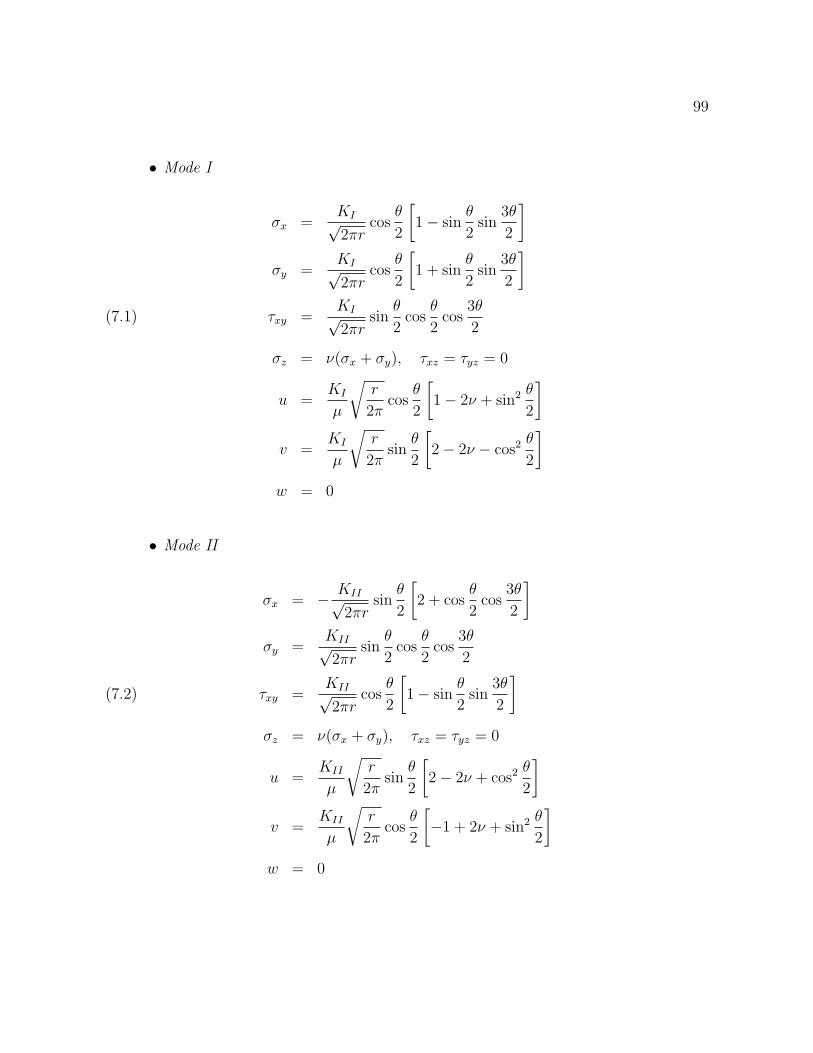
99

• Mode I

σx =KI√2πr

cosθ

2

[1− sin

θ

2sin

3θ

2

]

σy =KI√2πr

cosθ

2

[1 + sin

θ

2sin

3θ

2

]

τxy =KI√2πr

sinθ

2cos

θ

2cos

3θ

2(7.1)

σz = ν(σx + σy), τxz = τyz = 0

u =KI

µ

√r

2πcos

θ

2

[1− 2ν + sin2 θ

2

]

v =KI

µ

√r

2πsin

θ

2

[2− 2ν − cos2 θ

2

]

w = 0

• Mode II

σx = − KII√2πr

sinθ

2

[2 + cos

θ

2cos

3θ

2

]

σy =KII√2πr

sinθ

2cos

θ

2cos

3θ

2

τxy =KII√2πr

cosθ

2

[1− sin

θ

2sin

3θ

2

](7.2)

σz = ν(σx + σy), τxz = τyz = 0

u =KII

µ

√r

2πsin

θ

2

[2− 2ν + cos2 θ

2

]

v =KII

µ

√r

2πcos

θ

2

[−1 + 2ν + sin2 θ

2

]

w = 0

100

• Mode III

τxz = − KIII√2πr

sinθ

2

τyz =KIII√2πr

cosθ

2

σx = σy = σz = τxy = 0(7.3)

w =KIII

µ

√2r

πsin

θ

2

u = v = 0

where the stress components, σij, and the coordinates r and θ are shown in Figure 7.4;

u, v, and w are the displacements in the x−, y−, and z−directions, respectively; ν is

Poisson’s ratio, and µ is the shear modulus of elasticity.

Note that dimensional analysis of Eqs. 7.1, 7.2, and 7.3 must be related to the magnitude

of applied stress, and the square root of the crack length.

More details of the above with reference to the examples can be found in Tada et al.

(1973) [31], Hertzberg (1996) [23], and Barsom and Rolfe (1999) [39].

7.3. J-integral

In the previous section, we have introduced the basic principles of the stress intensity

factors (K).

The J-integral is widely accepted as a fracture mechanics parameter for both linear

and nonlinear material response. It is related to the energy release associated with crack

growth and is a measure of the intensity of deformation at a crack tip. Because of the

importance of the J-integral in the assessment of flaws, its accurate numerical evaluation is

101

θ

y

σ

σ

y

σx z

r

z

x

Leading edge of the crack

Figure 7.4. Stress components ahead of crack

vital to the practical application of fracture mechanics in design calculations. ABAQUS

provides a procedure for such evaluation of the J-integral, based on the virtual crack

extension/domain integral methods mentioned above. Further details can be found in

Parks, 1977 [42], Shih, Moran, and Nakamura, 1986 [43], Moran and Shih, 1987 [28] and

[29], and ABAQUS manuals (2003) [2].

For a two-dimensional, planar, using the small displacement gradient assumption and

with body forces neglected, the path-independent J-integral is defined by (Rice, 1968

[44]),

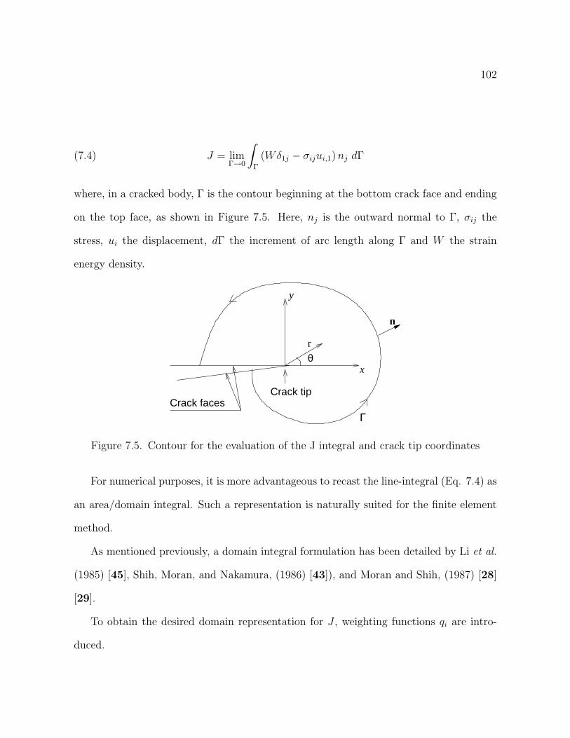
102

(7.4) J = limΓ→0

∫

Γ

(Wδ1j − σijui,1) nj dΓ

where, in a cracked body, Γ is the contour beginning at the bottom crack face and ending

on the top face, as shown in Figure 7.5. Here, nj is the outward normal to Γ, σij the

stress, ui the displacement, dΓ the increment of arc length along Γ and W the strain

energy density.

x

y

Crack tip

r

ΓCrack faces

n

θ

Figure 7.5. Contour for the evaluation of the J integral and crack tip coordinates

For numerical purposes, it is more advantageous to recast the line-integral (Eq. 7.4) as

an area/domain integral. Such a representation is naturally suited for the finite element

method.

As mentioned previously, a domain integral formulation has been detailed by Li et al.

(1985) [45], Shih, Moran, and Nakamura, (1986) [43]), and Moran and Shih, (1987) [28]

[29].

To obtain the desired domain representation for J , weighting functions qi are intro-

duced.

103

y

x

A

j

jm

n

0C

−C

+C

jm

Γ

Figure 7.6. Convention at crack tip. Domain A is enclosed by Γ, C+, C−,and C0

For two-dimensional problems with the crack line oriented in the x-direction, q1 is the

only nonzero function and it has the value of unity on the contour Γ and zero on the

outer contour C0 (see Figure 7.6).

The integral in Eq. 7.4 can be restated as a line integral over the closed contour C,

which consists of Γ, C0, and the crack faces C+ and C−, by

(7.5) J =

∫

C

(Wδ1j − σij ui1) mjq1dC

here, mj are the components of the unit vectors normal to C. On the contour Γ, mj is

equal to the negative of nj which has been defined earlier in Eq. 7.4.

Applying the divergence theorem to Eq. 7.5, we obtain,

104

(7.6) J =

∫

A

[σijui,1 −Wδ1j] q1,jdA

where A is the area enclosed by the closed contour C.

Assuming that,

(7.7) P1j,j q1 = 0

It follows that,

(7.8)

∫

Ω

P1j,j q1 dΩ = 0

(7.9)

∫

Ω

[(P1j q1),j − P1jq1,j] dΩ = 0

With,

(7.10)

∫

Ω

P1jq1,j dΩ =

∫

∂Ω

P1jq1 mj dS

Thus,

(7.11)

∫

Ω

(P1j q1),j dΩ−∫

∂Ω

P1jq1 mj dS = 0

Or,

(7.12)

∫

∂Ω

P1jq1 mj dS =

∫

Ω

(P1j q1),j dΩ

105

Now, we apply this equation to the line contours,

(7.13)∫

Γ2

P1jq1 mj dS +

∫

Γ1

P1jq1 mj dS +

∫

C+

P1jq1 mj dS +

∫

C−P1jq1 mj dS =

∫

Ω

(P1j q1),j dΩ

Recalling that q1 = 0 on the outer contour Γ2 and q1 = 1 on the inner contour Γ1. Thus,

(7.14)

∫

Γ2

P1jq1 mj dS = 0

And,

(7.15)

∫

Γ1

P1jq1 mj dS =

∫

Γ1

P1j mj dS = −J

Therefore,

(7.16) J = −∫

Ω

(P1j q1),j dΩ +

∫

C+

P1jq1 mj dS +

∫

C−P1jq1 mj dS

Or,

(7.17) J = −∫

Ω

[Wδ1j − σijui,1] q1,j dΩ +

∫

C+

P1jq1 mj dS +

∫

C−P1jq1 mj dS

7.4. Model validation

We have validated the FEA 3D model for the linear elastic analysis (Chapter 3) and

the thermal model (Chapter 5). In a similar approach, we will conduct a series of tests

to validate the 3D crack model. The tests include checking the validity of a simplified 3D

model in which the geometry and results are available in literature. Among those most

106

commonly cited are the solutions to the problem of a planar elliptical cracks subjected to

Mode I loading, provided by Raju and Newman (1979) [26].

7.4.1. Contour integral evaluation of a simplified 3D model

The geometry is shown in Figure 7.8. The model is loaded in Mode I by far-field tension.

Due to symmetry, only one-quarter of the geometry needs to be analyzed. To simplify we

will call our FEA model a benchmark model. We will compare the benchmark model ver-

sus Raju and Newman model (also called “Newman-Raju” in the plot). The comparison

of the computed Mode I SIFs is shown in Figure 7.7.

0

100

200

300

400

500

600

0 10 20 30 40 50 60 70 80 90

Crack front location, [degrees]

SIF

: K

I, [

lb/i

n^

2-i

n^

1/2

]

Raju-Newman Benchmark

Figure 7.7. Comparison of computed Mode I stress intensity factors

107

(Ave. Crit.: 75%)S, Mises

+2.739e+01+3.889e+01+5.040e+01+6.190e+01+7.341e+01+8.491e+01+9.642e+01+1.079e+02+1.194e+02+1.309e+02+1.424e+02+1.539e+02+1.654e+02

1

2

3

Figure 7.8. Mesh for semi-elliptic crack problem

The FEA stress intensity factors, KI , along the crack line are compared with those

obtained by Raju and Newman, 1979 [26] (Figure 7.7), who used a nodal force method

to compute KI from a finite element solution. The comparison shows good agreement

between the results. Here, the J-integral values are converted to KI using the formulation,

J =1− ν2

EK2

I

where ν is the Poisson’s ratio and E is the Young’s modulus.

It is important to note that our present benchmark model uses first-order reduced-

integration brick element (C3D8R), similar to the bridge model. Consequently, by using

the same type of element and the same type of meshing (without singular elements), we

108

can verify the accuracy level in 3D crack modeling applied to the bridge. Note that if

we use rather a quadratic element (20-node element) and singular elements with mid-side

nodes moved to the quarter position on element edges that focus onto the crack tip nodes,

the FEA results are very closed to the reference results.

The main reasons are:

• For a multi-body contact problem; i.e. joint connection of the bridge, the first-

order brick element (8-node element) is recommended. The KI values provided

by 8-node brick element show some “oscillation” at the beginning of the crack

front. This minor loss of accuracy is assumed to be attributable to the type of

element used (linear rather than quadratic) and without singular type of element.

However, the final results, as depicted in Figure 7.7, are reasonably closed to the

reference model (as suggested by Raju and Newman (1979) [26]). They are about

8% for φ = 0 and 5% for φ = 90.

• The current version of ABAQUS, (ABAQUS 6.4-5, 2003) [2], does not have the

capability to produce automatically the singular elements near the crack tip with

the pre-processor ABAQUS/CAE. An alternative solution is to mesh by hand.

However, due to the complex geometry of the bridge model, this alternative is

not feasible.

7.5. FEA prediction of the mixed-mode SIFs on operating conditions

Let us recall the operating conditions mentioned previously:

• unlocked condition

• locked condition

109

Note that “locked” condition signifies no relative motion is allowed between part compo-

nents; e.g. web girder and pin and hanger plate and pin. This means that each pair of

them is assumed to stick together in perfect “bonding”. This particular condition is used

to simulate the existence and formation of the “pack-rust” inside the joints.

7.5.1. Unlocked conditions

In this section, the elements of the connection are allowed to move freely relative to each

other. This is an idealistic condition which pertains mostly to the new bridges. However,

for aging bridges, there are some degrees of “lockup” inside the joint connections.

X

Y

Z

Local deformation near the crack surfaces (due to compression)

Figure 7.9. Local deformation near the crack surfaces due to compression(bottom pin)

110

7.5.1.1. Effects of temperature changes. The main objective here is to explore

whether there are linear relationships between the temperatures and the stress inten-

sity factors. Remember that bridge elements expand and contract due to temperature

changes (daily and seasonal changes). In the present model, the initial (or ambient tem-

perature) was set to be T0 = 59 F (15 C). Then, we increase linearly the temperatures;

e.g. T = 86 F (30 C), and T = 113 F (45 C). We would expect to obtain the linear

relationships of the stress intensity factors based on these differential temperatures.

The American Association of State Highway and Transportation Officials specifica-

tion (AASHTO (1996) [11]) provides temperature variations depending on whether the

structure is in a moderate or cold climate region. For steel bridge structure similar to this

one, the values are given in the form of extreme cold and hot temperatures. The ranges

are −30 F (−34.4 C) and 120 F (48.9 C) (see Table 7.1).

Table 7.1. AASHTO temperature ranges

From To

Moderate climate 0F 120FCold climate −30F 120F

The FEA results are shown in Figures 7.12, 7.13, 7.14, and 7.15. The plots indicate

that the stress intensity factors increase when the temperature increase. These are mainly

due to the movements of the bridge components as a result of their expansions or contrac-

tions. In addition, we also found that there is a linearity in the effective stress intensity

factor (Keff ) versus temperature (see Figure 7.15).

The definition of local orthogonal cartesian coordinates at the point s on the crack

front is illustrated in Figure 7.10. The schematic representation shows the the unit vectors

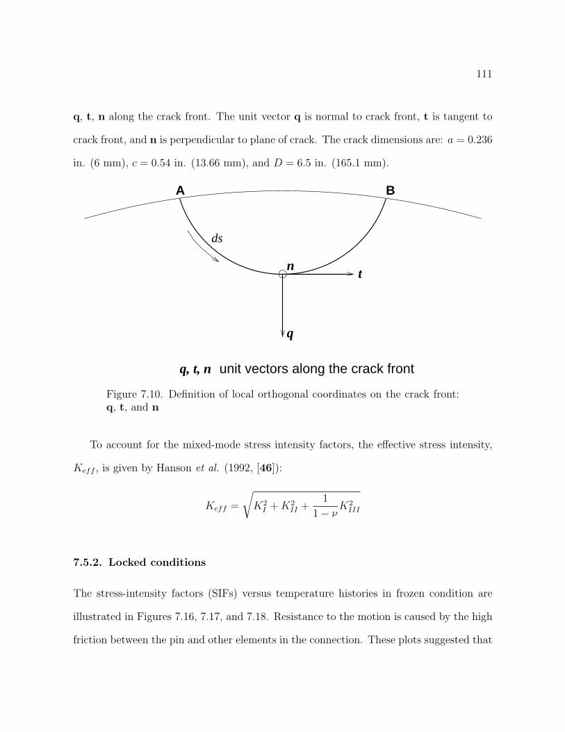
111

q, t, n along the crack front. The unit vector q is normal to crack front, t is tangent to

crack front, and n is perpendicular to plane of crack. The crack dimensions are: a = 0.236

in. (6 mm), c = 0.54 in. (13.66 mm), and D = 6.5 in. (165.1 mm).

unit vectors along the crack frontq, t, n

t

q

n

ds

BA

Figure 7.10. Definition of local orthogonal coordinates on the crack front:q, t, and n

To account for the mixed-mode stress intensity factors, the effective stress intensity,

Keff , is given by Hanson et al. (1992, [46]):

Keff =

√K2

I + K2II +

1

1− νK2

III

7.5.2. Locked conditions

The stress-intensity factors (SIFs) versus temperature histories in frozen condition are

illustrated in Figures 7.16, 7.17, and 7.18. Resistance to the motion is caused by the high

friction between the pin and other elements in the connection. These plots suggested that

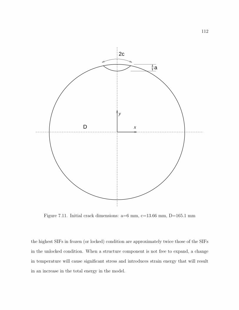
112

D

a

2c

y

x


the highest SIFs in frozen (or locked) condition are approximately twice those of the SIFs

in the unlocked condition. When a structure component is not free to expand, a change

in temperature will cause significant stress and introduces strain energy that will result

in an increase in the total energy in the model.

113

-6.0E+07

-4.0E+07

-2.0E+07

0.0E+00

2.0E+07

4.0E+07

6.0E+07

8.0E+07

1.0E+08

5 30 55 80 105 130 155

Crack front locations, [deg.]

SIF

s:

KI, K

II, K

III, K

eff

, [

SI u

nit

s]

KI KII KIII Keff

Figure 7.12. Mixed-mode SIFs (unlocked) for temperature T = 15 C (T =59 F)

Note the high torsion response on the pin surface due to frozen (locked) condition.

Also note the difference movement between expansion and contraction.


The above results suggest that the mixed-mode stress intensity factors KI , KII , and

KIII are higher at the beginning and at the end of the crack front. The highest values on

these locations are mainly due to the direct contact pressure (compression) applied by the

web girder to the pin. However, in the center portion along the crack front, the SIFs are

much lower (far away from the direct contact pressure). Furthermore, the SIFs are fairly

linear versus temperatures in unlocked conditions. They are not in locked conditions.

114

-1.0E+08

-7.5E+07

-5.0E+07

-2.5E+07

0.0E+00

2.5E+07

5.0E+07

7.5E+07

1.0E+08

5 30 55 80 105 130 155


SIF

s:

KI, K

II, K

III, K

eff

, [S

I u

nit

s]

KI KII KIII Keff


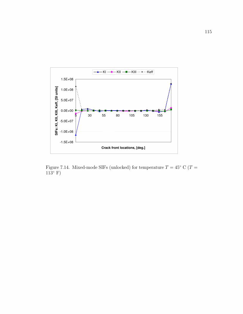
115

-1.5E+08

-1.0E+08

-5.0E+07

0.0E+00

5.0E+07

1.0E+08

1.5E+08

5 30 55 80 105 130 155


SIF

s:

KI, K

II, K

III, K

eff

, [S

I u

nit

s]

KI KII KIII Keff


116

0.0E+00

2.0E+07

4.0E+07

6.0E+07

8.0E+07

1.0E+08

1.2E+08

1.4E+08

5 30 55 80 105 130 155


SIF

eff

ec

tiv

e, K

eff

, [S

I u

nit

s]

Keff-15 Keff-30 Keff-45

Figure 7.15. Effective SIF (unlocked), Keff for different temperatures

117

-1.0E+08

-8.0E+07

-6.0E+07

-4.0E+07

-2.0E+07

0.0E+00

2.0E+07

4.0E+07

6.0E+07

8.0E+07

1.0E+08

1.2E+08

5 30 55 80 105 130 155


SIF

s:

KI, K

II, K

III, K

eff

, [S

I u

nit

s]

KI KII KIII Keff

Figure 7.16. Mixed-mode SIFs (locked) for temperature T = 15 C (T =59 F)

118

-2.0E+08

-1.5E+08

-1.0E+08

-5.0E+07

0.0E+00

5.0E+07

1.0E+08

1.5E+08

2.0E+08

2.5E+08

5 30 55 80 105 130 155


SIF

s:

KI, K

II, K

III, K

eff

, [S

I u

nit

s]

KI KII KIII Keff


119

-3.0E+08

-2.0E+08

-1.0E+08

0.0E+00

1.0E+08

2.0E+08

3.0E+08

4.0E+08

5 30 55 80 105 130 155


SIF

s:

KI, K

II, K

III, K

eff

, [S

I u

nit

s]

KI KII KIII Keff


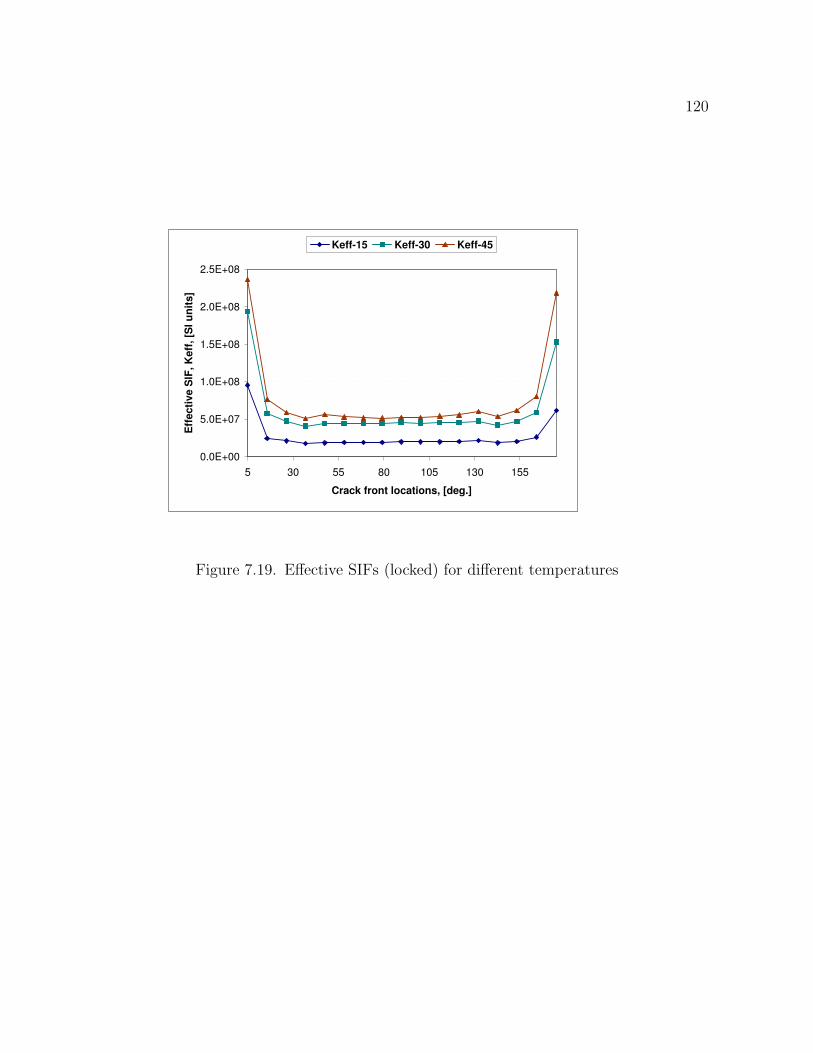
120

0.0E+00

5.0E+07

1.0E+08

1.5E+08

2.0E+08

2.5E+08

5 30 55 80 105 130 155


Eff

ecti

ve S

IF, K

eff

, [S

I u

nit

s]

Keff-15 Keff-30 Keff-45

Figure 7.19. Effective SIFs (locked) for different temperatures

121

0.0E+00

5.0E+07

1.0E+08

1.5E+08

2.0E+08

2.5E+08

5 30 55 80 105 130 155


Eff

ecti

ve S

IFs, K

eff

, [S

I u

nit

s]

Keff-unlocked Keff-locked

Figure 7.20. Comparison between effective SIFs between unlocked andlocked conditions

122

Combined loading: Torsion, Shear, Bending

Crack front

T

B

S

T

BA

Figure 7.21. Schematic diagram of the combined loading

123

(Avg: 75%)S, Mises

+2.306e+07+1.512e+08+2.794e+08+4.076e+08+5.357e+08+6.639e+08+7.921e+08+9.202e+08+1.048e+09+1.177e+09+1.305e+09+1.433e+09+1.561e+09

XY

Z

Cracked Pin

T=45C (expansion)

BA

Figure 7.22. Stress contour for a temperature T=45C

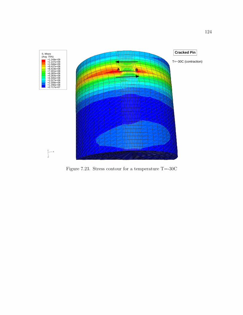
124

(Avg: 75%)S, Mises

+2.717e+07+1.290e+08+2.309e+08+3.327e+08+4.345e+08+5.364e+08+6.382e+08+7.401e+08+8.419e+08+9.437e+08+1.046e+09+1.147e+09+1.249e+09

XY

Z

A B

Cracked Pin

T=−30C (contraction)

Figure 7.23. Stress contour for a temperature T=-30C

125

CHAPTER 8

Computational modeling of fatigue crack growth

8.1. Introduction

This chapter investigates computational modeling of fatigue crack growth in the cylin-

drical shaped pin, which is one of the critical components of the joint connection. It

should be noted that crack growth simulation is the process of modeling crack evolution

in a structure. This includes all aspects of the modeling process from initial model prepa-

ration to visualization of results. This leads to the prediction of crack growth and the

evaluation of structural integrity. Therefore, crack growth simulation is an incremental

process, where a series of steps is repeated. Although, ABAQUS has an automatic mesh

generation capability (ABAQUS/CAE), construction of a proper 3D crack model requires

some human intervention and certain skills from the analyst.

In the simulation of the fatigue crack propagation, stress intensity factors (SIFs) are

required for use in the crack growth law. The SIFs, computed in the previous Chapter,

are augmented here by an algorithm to calculate crack growth, under cyclic loading. The

computation of the SIFs along the three-dimensional crack front remains a challenging

problem. This is primarily due to the fact that accurate calculation of stress intensity

factors (SIFs) in engineering applications has been a non-trivial task.

Prior to this study, there were not many examples of 3D crack growth work on cylindri-

cal pin with transverse crack. Furthermore, moving and combined loads due to multibody

126

contacts had not been considered in these previous analyses. The absence of closed-form

solutions add to the list of difficulty during the investigation.

Motivated by this challenging problem and its difficulty, and a number of other similar

problems in industry, several enhancements have been made. These include add-on tools

for evaluating the crack growth.

8.2. Computational procedure for evaluating the crack growth

The basic procedure for estimating the fatigue life of a structure from a fracture

mechanics approach is to first estimate the initial crack geometry and the critical crack

size. Next, the number of cycles required to grow the crack from the initial size to the

critical size is calculated. Once the number of load cycles is known, the time required to

accumulate that many cycles is calculated from the average daily truck traffic. It takes

time for a fatigue crack to develop. But a crack can then expand rapidly to become a

fracture.

8.3. Crack growth simulation in ABAQUS

As mentioned before, the version of ABAQUS (version 6.4.5) [2], used in this inves-

tigation, does not have crack propagation capabilities in 3D. Therefore, an alternative

approach was used. Our current approach consists in creating add-on tools, which com-

bine with the Paris’s power law for fatigue crack growth, to be used in conjunction with the

ABAQUS program. Fatigue crack growth rates were correlated with the stress intensity

factor ranges.

Although, ABAQUS has an automatic mesh generation capability (ABAQUS/CAE),

construction of a proper 3D crack model requires some human intervention. Considering

127

the complexities involved in fatigue modeling in engineering applications, the predictions

of the finite element analysis (FEA) appear to be reasonable in an engineering sense.

8.4. Fatigue crack growth

Figure 8.1 illustrates the initial crack geometry. The elevation view shows the initial

crack on the pin surface, located on the shear plane between the suspended web-girder

and the hanger plate. Due to cyclic loading generated by the traffic, this crack can grow

over a period of time until the crack extends through the pin section. This can lead to

catastrophic consequences, as we mentioned earlier.

X

Y

Z

Initial crack

Figure 8.1. Initial crack profile embedded on the pin surface

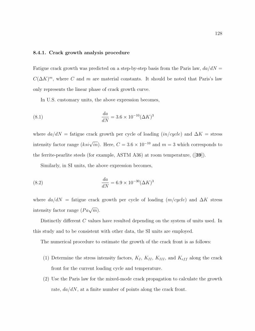
128

8.4.1. Crack growth analysis procedure

Fatigue crack growth was predicted on a step-by-step basis from the Paris law, da/dN =

C(∆K)m, where C and m are material constants. It should be noted that Paris’s law

only represents the linear phase of crack growth curve.

In U.S. customary units, the above expression becomes,

(8.1)da

dN= 3.6× 10−10(∆K)3

where da/dN = fatigue crack growth per cycle of loading (in/cycle) and ∆K = stress

intensity factor range (ksi√

in). Here, C = 3.6× 10−10 and m = 3 which corresponds to

the ferrite-pearlite steels (for example, ASTM A36) at room temperature, ([39]).

Similarly, in SI units, the above expression becomes,

(8.2)da

dN= 6.9× 10−30(∆K)3

where da/dN = fatigue crack growth per cycle of loading (m/cycle) and ∆K stress

intensity factor range (Pa√

m).

Distinctly different C values have resulted depending on the system of units used. In

this study and to be consistent with other data, the SI units are employed.

The numerical procedure to estimate the growth of the crack front is as follows:

(1) Determine the stress intensity factors, KI , KII , KIII , and Keff along the crack

front for the current loading cycle and temperature.

(2) Use the Paris law for the mixed-mode crack propagation to calculate the growth

rate, da/dN , at a finite number of points along the crack front.

129

(3) Assign the number of cycles, ∆N .

(4) The increase in crack length da is then computed along the crack front.

(5) To determine the new front of the crack, we need to calculate the coordinates of

a vector normal of a finite number of points along the crack front. The details

can be found in the following section.

(6) Similarly, to determine the positions of the end points (on the circle), we need

to calculate their coordinates by using polar coordinates. Further details can be

found in the subsequent section as well.

(7) Repeat (1)-(6) for the evolving crack.

As discussed above, the rate of fatigue crack growth under cyclic loading can be

expressed in terms of range of stress intensity factor through Paris’s power law (Paris,

1963 [47]),

(8.3)da

dN= C(∆Keff )

m

where C and m are 2 coefficients which depend on the material resistance. N is the cycle

number. For a mixed-mode loading, the range of the effective stress intensity factor, Keff ,

is used, which can be obtained according to the expression,

(8.4) ∆Keff =

√∆K2

I + ∆K2II +

1

1− ν∆K2

III

130

where ∆K is the difference between maximum and minimum stress intensity factors during

a loading cycle. The equation (8.3) implies that da/dN depends on ∆Keff only, where

∆Keff =

√∆K2

I + ∆K2II +

1

1− ν∆K2

III(8.5)

da

dN= C(∆Keff )

m(8.6)

∆ak = C(∆Kkeff )

m k = 1, npoints(8.7)

∆N =(∆a)max

C (∆Kmaxeff )m

(8.8)

8.4.2. New contour crack front computations

This section describes the integration of add-on tools to be used in conjunction with the

ABAQUS program.

As mentioned earlier, in order to determine the new crack front, we first need to

calculate the coordinates of a vector normal to a parabolic section. The parabola is an

approximated curve of the crack front. It is defined by 3 points on a plane. We need to

calculate the coordinates of the end points of the normal vector. These will be combined

to the increase in crack length ∆a, previously calculated.

8.4.2.1. New crack front normal positions. In order to determine the coordinates

of the points which constitute the new crack front, we need to calculate the coordinates

of a vector normal to a parabola (Figure 8.3), which represents the current position of

the crack front.

The equation of the parabola is y = ax2 + bx + c. Let us set up three equations in

three unknowns using the coordinates of three points; i.e. points 1, 2, and 3:

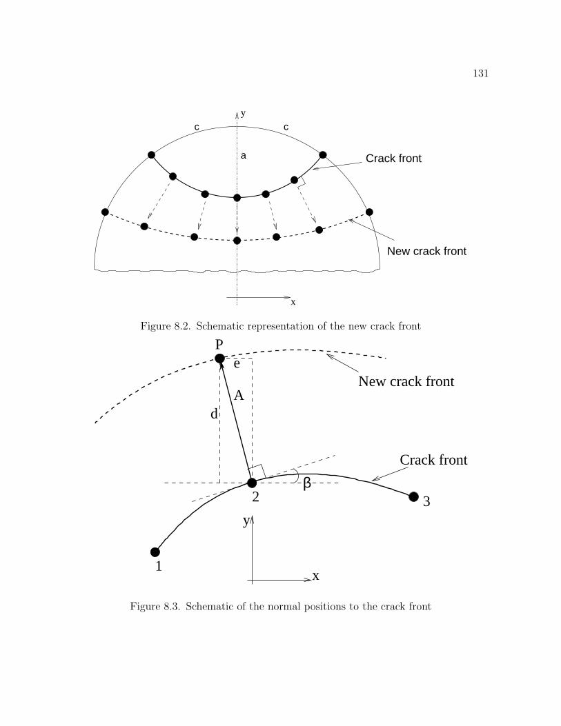
131

x

y

cc

a Crack front

New crack front

Figure 8.2. Schematic representation of the new crack front

3

1

2

P

d

y

β

A

Crack front

New crack front

x

e

Figure 8.3. Schematic of the normal positions to the crack front

132

y1 = ax21 + bx1 + c

y2 = ax22 + bx2 + c

y3 = ax23 + bx3 + c

Now, let us solve these 3 equations for the unknowns, a, b, and c. From the calculus,

the slope m of the parabola at (x2, y2) is defined as,

m = 2ax2 + b = tan β

For notations used here, refer to Figure 8.3,

d = A cos β

sin2 β + cos2 β = 1

tan2 β + 1 =1

cos2 β

cos β =1√

1 + tan2 β

=1√

1 + m2

Since,

d = A cos β

133

Thus,

d = A cos β

=A√

1 + m2

Similarly,

e = A sin β

= Am× 1√1 + m2

= md

Depending on whether the normal has a positive or negative y component determines

whether the end point of the normal will be,

xN = x2 −md

yN = y2 + d

or whether,

xN = x2 + md

yN = y2 − d

8.4.2.2. New crack front end-points located on the circle. In order to determine

the positions of the end points located on the circle section, we use an approach which

consists to express the coordinates of these points in polar coordinates (see Figure 8.4).

134

P

O

c

R

θα

y

x

a∆

Crack front

Figure 8.4. New crack front end-points located on the circle

The coordinates of point c are,

xc = x0 + R cos α

yc = y0 + R sin α

Similarly, the coordinates of point P are,

xP = x0 + R cos θ

yP = y0 + R sin θ

135

The increase in crack length ∆a is then computed as,

(xP − xc)2 + (yP − yc)

2 = ∆a2

(x0 + R cos θ − x0 −R cos α)2 + (y0 + R sin θ − y0R sin α)2 = ∆a2

R2[(cos θ − cos α)2 + (sin θ − sin α)2

]= ∆a2

cos(θ − α) = 1− ∆a2

2R2

Hence,

θ = α± cos−1

(1− ∆a2

2R2

)

Therefore, the coordinates of the new end-points located on the circle are,

xP = x0 + R cos θ

yP = y0 + R sin θ

8.4.3. Results

This section illustrates the results of the computations using the step-by-step procedure,

as previously described, to predict the fatigue crack growth in the pin component.

The main question concerning fatigue crack growth is “how long does it take for a crack

to grow from a certain initial size (a0) to a critical size (acr)?” The initial crack size, a0,

typically corresponds to the size that can be detected using non-destructive inspection

techniques (NDT). The critical size may be the size at which the stress intensity factor

exceeds the fracture toughness at some point along the crack front or it may be some

predetermined size for assessment and comparative purposes.

136

1561 1560

1559

1558

1557

1556

1555

1554

1553

1552

1551

1550

1549

1548 1547

1201

1200

1199

1198

1197

1196

1195

1194

1193

1192

1191

1190

1189

1188

1187

451

450

449

448

447

313

312 311

310

309

271

270

269

268

267

185

184

183

182

181

180

179

178

131

130

129

128

127

126

125

63

62 61

60 59 58 57

18 13

10

4

1

(Avg: 75%)S, Mises

+5.352e+07+1.250e+08+1.964e+08+2.679e+08+3.393e+08+4.108e+08+4.822e+08+5.537e+08+6.251e+08+6.966e+08+7.681e+08+8.395e+08+9.110e+08

X

Y

Z

Crack front

Figure 8.5. Crack surfaces

8.4.3.1. Prediction of fatigue crack growth. As said before, the criterion of crack

propagation is based on the Paris law (Paris, 1963 [47]). To account for the mixed-mode

propagation, the stress intensity factor is given by:

∆Keff =

√(K

(1)I −K

(0)I )2 + (K

(1)II −K

(0)II )2 +

1

1− ν(K

(1)III −K

(0)III)

2

where ∆K is the difference between the maximum and the minimum stress intensity

factors during a loading cycle. Here, the maximum corresponds to the total load, which

includes dead load, live load, and thermal load. The minimum corresponds to the dead

load.

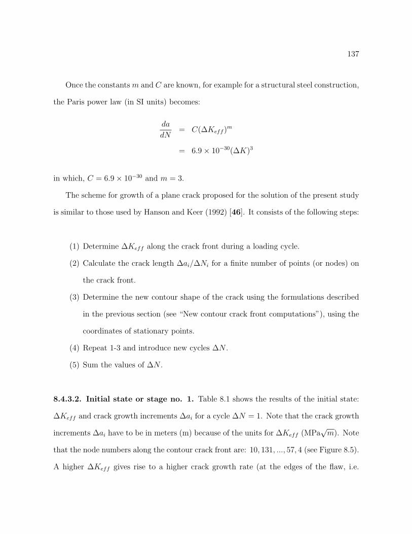
137

Once the constants m and C are known, for example for a structural steel construction,

the Paris power law (in SI units) becomes:

da

dN= C(∆Keff )

m

= 6.9× 10−30(∆K)3

in which, C = 6.9× 10−30 and m = 3.

The scheme for growth of a plane crack proposed for the solution of the present study

is similar to those used by Hanson and Keer (1992) [46]. It consists of the following steps:

(1) Determine ∆Keff along the crack front during a loading cycle.

(2) Calculate the crack length ∆ai/∆Ni for a finite number of points (or nodes) on

the crack front.

(3) Determine the new contour shape of the crack using the formulations described

in the previous section (see “New contour crack front computations”), using the

coordinates of stationary points.

(4) Repeat 1-3 and introduce new cycles ∆N .

(5) Sum the values of ∆N .

8.4.3.2. Initial state or stage no. 1. Table 8.1 shows the results of the initial state:

∆Keff and crack growth increments ∆ai for a cycle ∆N = 1. Note that the crack growth

increments ∆ai have to be in meters (m) because of the units for ∆Keff (MPa√

m). Note

that the node numbers along the contour crack front are: 10, 131, ..., 57, 4 (see Figure 8.5).

A higher ∆Keff gives rise to a higher crack growth rate (at the edges of the flaw, i.e.

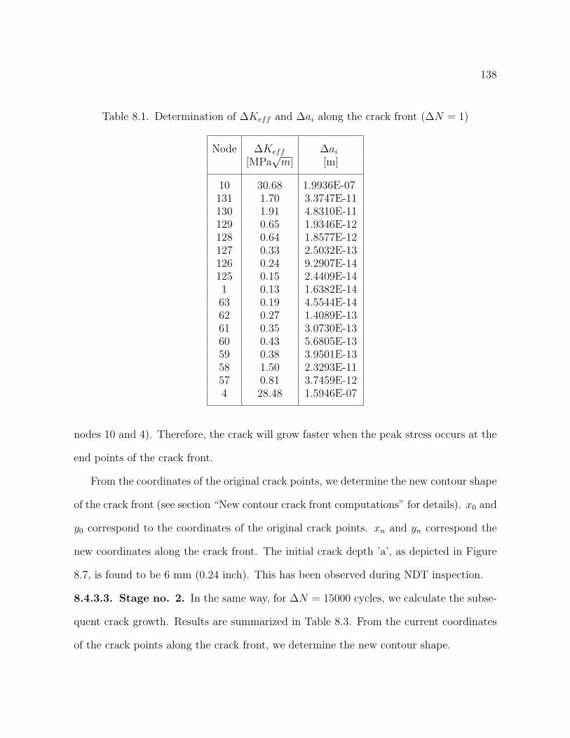
138

Table 8.1. Determination of ∆Keff and ∆ai along the crack front (∆N = 1)

Node ∆Keff ∆ai

[MPa√

m] [m]

10 30.68 1.9936E-07131 1.70 3.3747E-11130 1.91 4.8310E-11129 0.65 1.9346E-12128 0.64 1.8577E-12127 0.33 2.5032E-13126 0.24 9.2907E-14125 0.15 2.4409E-141 0.13 1.6382E-1463 0.19 4.5544E-1462 0.27 1.4089E-1361 0.35 3.0730E-1360 0.43 5.6805E-1359 0.38 3.9501E-1358 1.50 2.3293E-1157 0.81 3.7459E-124 28.48 1.5946E-07

nodes 10 and 4). Therefore, the crack will grow faster when the peak stress occurs at the

end points of the crack front.

From the coordinates of the original crack points, we determine the new contour shape

of the crack front (see section “New contour crack front computations” for details). x0 and

y0 correspond to the coordinates of the original crack points. xn and yn correspond the

new coordinates along the crack front. The initial crack depth ’a’, as depicted in Figure

8.7, is found to be 6 mm (0.24 inch). This has been observed during NDT inspection.

8.4.3.3. Stage no. 2. In the same way, for ∆N = 15000 cycles, we calculate the subse-

quent crack growth. Results are summarized in Table 8.3. From the current coordinates

of the crack points along the crack front, we determine the new contour shape.

139

Table 8.2. New crack front coordinates (∆N = 1)

Node x0 y0 xn yn

10 -0.01367 0.08141 -0.01367 0.08141131 -0.01218 0.08032 -0.01218 0.08032130 -0.01060 0.07936 -0.01060 0.07936129 -0.00895 0.07853 -0.00895 0.07853128 -0.00724 0.07784 -0.00724 0.07784127 -0.00548 0.07729 -0.00548 0.07729126 -0.00367 0.07688 -0.00367 0.07688125 -0.00184 0.07663 -0.00184 0.076631 0. 0.07655 0. 0.0765563 0.00184 0.07663 0.00184 0.0766362 0.00367 0.07688 0.00367 0.0768861 0.00548 0.07729 0.00548 0.0772960 0.00724 0.07784 0.00724 0.0778459 0.00895 0.07853 0.00895 0.0785358 0.01060 0.07936 0.01060 0.0793657 0.01218 0.08032 0.01218 0.080324 0.01367 0.08141 0.01367 0.08141

8.4.3.4. Stage no. 3. Results are summarized in Table 8.5 for a new increment of

∆N = 10000. The new crack front is illustrated in Table 8.6.

Based on the step-by-step calculations, as shown above (stage no.1, stage no. 2, and

stage no. 3), the number of cycles was found to be N = 25, 001. We observe that ∆Keff

is higher at the edges of the flaw; i.e. nodes 10 and 4. Therefore, the crack will grow faster

when the peak stress occurs at these end points of the crack front. The crack dimension c

was initially measured as c = 13.66 mm (see Figure 8.7). At N = 25001 cycles, c = 19.22

mm.

The number of cycles, N = 25001 for this amount of crack growth, corresponds ap-

proximately to 68 years if the joints of the bridge are completely unlocked. On the other

140


Node ∆Keff ∆ai

[MPa√

m] [m]

10 30.69 0.00299131 1.69 5.03787E-07130 1.91 7.24210E-07129 0.65 2.91629E-08128 0.65 2.79232E-08127 0.33 3.75367E-09126 0.24 1.38816E-09125 0.15 3.66135E-101 0.13 2.45680E-1063 0.19 6.83297E-1062 0.27 2.10485E-0961 0.35 4.62898E-0960 0.43 8.54081E-0959 0.38 5.92556E-0958 1.50 3.49328E-0757 0.81 5.56189E-084 28.52 0.00240

hand, it was found that the maximum stress intensity factor under locked conditions is

about 2 times higher than under unlocked conditions (see plot 7.20 in Chapter 7). Accord-

ingly, it was estimated that 9 years should correspond to the locked conditions. Therefore,

the reduction in time to growth (locked versus unlocked) is indicative of severity of locked

case, although the crack was not grown to failure in the present analysis.


We have established a framework for assessment of structural integrity and fatigue

life of pin and hanger connections. The relatively complex way in which the crack length

141

Table 8.4. New crack front (∆N = 15000)

Node x0 y0 xn yn

10 -0.01367 0.08141 -0.01661 0.08086131 -0.01218 0.08032 -0.01218 0.08032130 -0.01060 0.07936 -0.01060 0.07936129 -0.00895 0.07853 -0.00895 0.07853128 -0.00724 0.07784 -0.00724 0.07784127 -0.00548 0.07729 -0.00548 0.07729126 -0.00367 0.07688 -0.00367 0.07688125 -0.00184 0.07663 -0.00184 0.076631 0. 0.07655 0. 0.0765563 0.00184 0.07663 0.00184 0.0766362 0.00367 0.07688 0.00367 0.0768861 0.00548 0.07729 0.00548 0.0772960 0.00724 0.07784 0.00724 0.0778459 0.00895 0.07853 0.00895 0.0785358 0.01060 0.07936 0.01060 0.0793657 0.01218 0.08032 0.01218 0.080324 0.01367 0.08141 0.01604 0.08098

must be determined for each load cycle and the step-by-step counting method of generating

crack growth requires long running times and tedious calculations.

Crack growth calculations were carried out for the unlocked case only. We estimate,

based on initial stress intensity factors for the locked case that the time to growth the

crack to c = 19.22 mm would be reduced by a factor of 2 from that in the unlocked case.

No attempt to grow the crack to failure was made and these calculations merely

serve to illustrate the severity of the locked case over that of the unlocked. More detail

investigations of the actual fatigue crack growth mechanisms would be required in order

to make statements about failure processes in actual bridge pins.

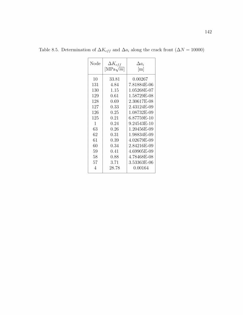
142


Node ∆Keff ∆ai

[MPa√

m] [m]

10 33.81 0.00267131 4.84 7.81884E-06130 1.15 1.05268E-07129 0.61 1.58729E-08128 0.69 2.30617E-08127 0.33 2.43124E-09126 0.25 1.08732E-09125 0.21 6.87759E-101 0.24 9.24543E-1063 0.26 1.20456E-0962 0.31 1.98834E-0961 0.39 4.02679E-0960 0.34 2.84216E-0959 0.41 4.69905E-0958 0.88 4.78468E-0857 3.71 3.53363E-064 28.78 0.00164

143

Table 8.6. New crack front (∆N = 10000)

Node x0 y0 xn yn

10 -0.01661 0.08086 -0.01922 0.08028131 -0.01218 0.08032 -0.01218 0.08032130 -0.01060 0.07936 -0.01060 0.07936129 -0.00895 0.07853 -0.00895 0.07853128 -0.00724 0.07784 -0.00724 0.07784127 -0.00548 0.07729 -0.00548 0.07729126 -0.00367 0.07688 -0.00367 0.07688125 -0.00184 0.07663 -0.00184 0.076631 0. 0.07655 0. 0.0765563 0.00184 0.07663 0.00184 0.0766362 0.00367 0.07688 0.00367 0.0768861 0.00548 0.07729 0.00548 0.0772960 0.00724 0.07784 0.00724 0.0778459 0.00895 0.07853 0.00895 0.0785358 0.01060 0.07936 0.01060 0.0793657 0.01218 0.08032 0.01218 0.080324 0.01604 0.08098 0.01765 0.08064

144

1

2

3

Figure 8.6. Deformed mesh showing new contour crack front

145

D

a

2c

y

x


146

CHAPTER 9

Conclusion and discussion

9.1. General discussions and recommendations

The aim of the present study was to investigate failure mechanisms of the pin and

hanger connections in aging highway steel bridges.

The aging of highway bridges is increasing the anxiety in all sectors of the industry,

particularly as there is a desire to operate the bridges beyond their original design lives.

Crack formation and growth in the vicinity of the joint connection has been identified as

a serious problem. The presence of cracks or flaws in complex three-dimensional compo-

nents is always a cause of concern to engineers. The frightening aspect of fatigue failure

mechanisms is that initial crack growth can often go undetected.

The aim also was to relate design calculations, originally performed in bridge design in

its earlier stage, to the entire structure behavior analysis carried out by our investigations.

Note that the design calculations were originally done in few single components; e.g.

tension in hanger, shear stress in the pin.

The advent of high speed computer has led to further advances in the use of numerical

method of stress analysis by means of the FEA. Furthermore, improved knowledge of

material behavior, plasticity, and mechanisms of fracture made possible the complete

analysis.

Based on the findings, the following conclusions can be drawn:

147

• Over-stressing. Plastic deformation occurred in several critical components, in

particular when the joints become completely frozen. Moments and high stress

concentration were generated from thermal expansion/contraction as well as live

loading once the pin was restrained from rotation. The mechanical freezing con-

dition of the lower pin can be attributed to the corrosion (pack-rust) due to salt

and debris accumulation. Furthermore, fatigue and reduction of fracture tough-

ness associated with low temperatures were among operating parameters to take

into account in design purpose. Therefore, better design of the pin and hanger

connection is required. Here are some basic recommendations:

(a) Partial sealing of the pin-and-hanger housing. This would help to prevent

salt and debris to accumulate near the joint.

(b) Greasing the lower and upper pins during regular inspections to ensure free

rotation of the links.

• Structurally deficient. It is also interesting to note that when the bridge was

designed (1954s), only a few part components were checked and compared to the

AASHTO specifications; i.e. tension in hanger, shear stress in pin. According to

the bridge design document, there is no indication on the effects of temperature

changes, nor the frozen condition inside the joints. The analyses are limited to

room temperature. The assumptions of the design calculations were mainly based

on an “idealistic” condition. Each connected element was assumed to freely rotate

relative to each other. In the present study, we found that the bridge elements are

over-stressed under the given applied loads and extreme environmental conditions

pertaining to the locked condition.

148

We would hope that advances in steel making, non-destructive evaluation, and numer-

ical procedure will promote to a better bridge design in the future.

9.1.1. Crack growth

The present study also has been focused on crack growth modeling. The focus was

performing 3D contact analysis of connecting elements incorporating crack. This is an

important concern since changes in contact loads may lead to changes in stress intensity

factors (SIFs) and therefore result in alteration of the crack front. This effect became

more noticeable as the crack grew.

It should be note that ABAQUS does not have the fatigue crack capability in its

current version. Therefore, the most significant feature that contributes to the simplicity

and efficiency use of the finite element program ABAQUS, for a crack growth modeling

in 3D, is a technique which allows for the calculation of the normal position for the new

crack front. It is implemented as an add-on tool for ABAQUS program.

We have established a framework for assessment of structural integrity and fatigue life

of pin and hanger connections. Our initial investigation gave preliminary but plausible

results on the effects of temperature fluctuations as well as mechanical lock up of the pins

on stress values and on susceptibility for crack growth.

Although, ABAQUS has an automatic mesh generation capability (ABAQUS/CAE),

construction of a proper 3D crack model requires some human intervention and a certain

skills from the analyst.

149

In addition, while the majority of complex geometries are still created with an under-

lying tetrahedral element, here we have had success by making our entire bridge model

with high quality brick shaped elements.

9.1.2. Non-destructive evaluation (NDE)

As mentioned earlier, most of the work and publications, on the assessment of aging

bridges, have been focused on non-destructive evaluation (NDE). Non-destructive testing

(NDT) or NDE of materials is an inspection procedure used to produce information

leading to decisions on the serviceability of components or structures. These procedures

are often complex requiring expensive equipment and skilled experts to operate efficiently.

Quantitative NDE techniques are needed for evaluating sizes, shapes, and locations of

defects and cracks. On the other hand, computational mechanics, in particular FEA, is a

tool for these tasks as well. Perhaps, the combination of these 2 tools should be used in

the future for an efficient assessment of the structural integrity of the bridge.

9.2. Future work

An automated crack growth program, as an add-on tool, for commercially available

FE program (ABAQUS) is needed if we want to use such commercial program in engi-

neering applications. An application program interface (API) using Python programming

language may be an appropriate way to do this. This may lead to an automatic global

remeshing for modeling crack propagation.

150

There is another possibility which consists to interface between the extended finite

element method (X-FEM) and ABAQUS. In the extended finite element method (X-

FEM), the approximation of the displacement field is enriched in the vicinity of the

crack by incorporating additional basis functions using a partition of unity approach. For

further details, see for example Sukumar et al. (2000) [48] and Sukumar et al. (2003)

[49], amongst others.

Finally, other aspect that could be included in the simulation is the corrosion. These

effects which cannot be easily incorporated (oxidation/corrosion) may enhance crack

growth.

151

References

[1] G. Chen, C. Courtright, L. R. Dharani, and B. Xu. Failure investigation of thesteel strut of Paseo suspension bridge. In Performing Organization Report. MissouriDepartment of Transportation (MoDOT), 2005.

[2] ABAQUS Inc. ABAQUS Manuals (version 6.45). HKS Inc., 2003.

[3] D. E. Kelsey and M. A. Rotundo. Ultrasonic Testing of Bridge Pins and HangerStraps. Materials Evaluation, pages 488–493, 1990.

[4] J. M. South, C. Hahin, and R. O. Telford. Analysis, Inspection, and Repair Methodsfor Pin Connections on Illinois Bridge. In Physical Research Report, volume 107.Illinois Department of Transportation (IDOT), 1992.

[5] R. A. Walther and R. D. Gessel. Ultrasonic Inspection of Bridge Pin and HangerAssemblies. In Proc. Structural Materials Technology, pages 23–28. San Diego, 1996.

[6] B. A. Graybeal, R. A. Walther, and G. A. Washer. Ultrasonic Inspection of BridgeHanger Pins. Transportation Research Record, 1697:19–23, 2000.

[7] D. E. Tonias and J. J. Zhao. Bridge Engineering. McGraw-Hill, 2nd edition, 2007.

[8] R. D. Cook, D. S. Malkus, and M. E. Plesha. Concepts and Applications of FiniteElement Analysis. John Wiley, 4th edition, 2002.

[9] M. R. Gosz. Finite Element Method - Applications in Solids, Structures, and HeatTransfer. CRC, 2006.

[10] F. K. Hubbard. Design Computations. Wisconsin Department of Transportation(WisDOT), 1999.

[11] American Association of State Highway and Transportation Officials (AASHTO).Standard Specifications for Highway Bridges. AASHTO, Washington D. C., 15thedition, 1996.

152

[12] T. Belytschko, W. K. Liu, and B. Moran. Nonlinear Finite Elements for Continuaand Structures. John Wiley, 2000.

[13] P. Wriggers. Computational Contact Mechanics. John Wiley, 2002.

[14] S. P. Timoshenko and J. N. Goodier. Theory of elasticity. McGraw-Hill, 2nd edition,1951.

[15] L. E. Malvern. Introduction to the Mechanics of a Continuous Medium. Prentice-Hall,1969.

[16] Y. C. Fung. Foundations of Solid Mechanics. Prentice-Hall, 1965.

[17] G. A. Holzapfel. Nonlinear Solid Mechanics: A Continuum Approach for Engineering.Wiley, 2000.

[18] R. Hill. The Mathematical Theory of Plasticity. Clarendon Press, 1950.

[19] D. R. J. Owen and E. Hinton. Finite elements in plasticity. Pineridge Press, U.K.,1980.

[20] M. A. Crisfield. Non-linear Finite Element Analysis of Solids and Structures. JohnWiley, 1991.

[21] A. S. Khan and S. Huang. Continuum Theory of Plasticity. John Wiley, 1995.

[22] C. W. Roeder. Proposed Design Method for Thermal Bridge Movements. Journal ofBridge Engineering, pages 12–19, 2003.

[23] R. W. Hertzberg. Deformation and Fracture Mechanics of Engineering Materials.John Wiley, 4th edition, 1996.

[24] A. P. Boresi and R. J. Schmidth. Advanced Mechanics of Materials. John Wiley, 5thedition, 2003.

[25] M. Gosz and B. Moran. Stress-intensity factors for elliptical cracks emanating fromcountersunk rivet holes. U.S. Dept. of Transportation - The FAA, 1998.

[26] I. S. Raju and J. C. Newman. Stress-intensity factors for a wide range of semi-ellipticalsurface cracks in finite-thickness plates. Eng. Fracture Mechanics, 11:817–829, 1979.

153

[27] J. C. Newman Jr. and I. S. Raju. Stress-intensity factor equations for cracks inthree-dimensional finite bodies. ASTM STP 791 - Fracture Mechanics, pages 238–265, 1983.

[28] B. Moran and C. F. Shih. A general treatement of crack tip contour integrals. Int.J. of Fracture, 35:295–310, 1987.

[29] B. Moran and C. F. Shih. Crack tip and associated domain integrals from momentumand energy balance. Eng. Fract. Mech., 27:615–642, 1987.

[30] J. Schijve. Fatigue of Structures and Materials. Kluwer Academic Publishers, 2001.

[31] H. Tada, P. C. Paris, and G. R. Irwin. The stress analysis of cracks handbook. DelResearch Corp., 1973.

[32] D. P. Rooke and D. J. Cartwright. Stress Intensity Factors. Her Majesty’s StationaryOffice, London, 1976.

[33] Y. Murakami (ed.). Stress Intensity Factors Handbook. Pergamon Press, Oxford,1987.

[34] I. S. Raju and J. C. Newman Jr. Stress-intensity factors for circumferential surfacecracks in pipes and rods under tension and bending loads. ASTM STP 905 - FractureMechanics, 17:789–805, 1986.

[35] M. Shiratori, T. Miyoshi, Y. Sakai, and G. R. Zhang. Analysis of stress intensityfactors for surface cracks subjected to arbitrarily distributed surface stresses. Trans.Jap. Soc. Mech. Eng., pages 660–662, 1986.

[36] Y. S. Shih and J. J. Chen. The stress intensity factor study of an elliptical crackedshaft. Nucl. Eng. and Des., 214:137–145, 2002.

[37] C. Q. Cai and C. S. Shin. A discussion on The stress intensity factor study of anelliptical cracked shaft. Nucl. Eng. and Des., 227:355–358, 2004.

[38] P. C. Paris and G. C. Sih. Stress Analysis of Cracks. In Fracture Toughness Testingand its Applications, ASTM STP 381. American Society for Testing and Materials(ASTM), Philadelphia, 1965.

[39] J. M. Barsom and S. T. Rolfe. Fracture and Fatigue Control in Structures. AmericanSociety for Testing and Materials, 3rd edition, 1999.

154

[40] H. M. Westergaard. Bearing Pressures and Cracks. In Transactions, ASME. Journalof Applied Mechanics, 1939.

[41] G. R. Irwin. Analysis of Stresses and Strains Near the End of a Crack Transversinga Plate. In Transactions, ASME, volume 24. Journal of Applied Mechanics, 1957.

[42] D. M. Parks. The virtual crack extension method for nonlinear material behavior.Comp. Meth. in Appl. Mech. Eng., 12:353–364, 1977.

[43] C. F. Shih, B. Moran, and T. Nakamura. Energy Release Rate along a Three-Dimensional Crack Front in a Thermally Stresed Body. J. of Appl. Mech., 30:79–102,1986.

[44] J. R. Rice. A Path Independent Integral and the Approximation Analysis of StrainConcentration by Notches and Cracks. J. of Appl. Mech., Transactions of ASME,35, 1968.

[45] F. Z. Li, C. F. Shih, and A. Needleman. A comparison of methods for calculatingenergy release rates. Eng. Fracture Mechanics, 21:405–421, 1985.

[46] M. T. Hanson and L. M. Keer. An Analytical Life Prediction Model for the CrackPropagation Occuring in Contact Fatigue Failure. Tribology Transactions, 35:451–461, 1992.

[47] P. C. Paris and F. Erdogan. A critical analysis of crack propagation laws. TransASME, Series D, 85:528–535, 1963.

[48] N. Sukuma, N. Moes, B. Moran, and T. Belytschko. Extended Finite ElementMethod (X-FEM) for Three-Dimensional Crack Modeling. Int. J. Num. Meth. inEng., 11:1549–1570, 2000.

[49] N. Sukuma, D. L. Chopp, and B. Moran. Extended Finite Element Method and FastMarching Method for Three-Dimensional Fatigue Crack Propagation. Eng. FractureMechanics, 70:29–48, 2003.

[50] American Institute of Steel Construction. Manual of Steel Construction. AISC,Chicago, 9 edition, 1992.

[51] F. P. Beer and E. R. Johnston. Mechanics of Materials. McGraw-Hill, 2nd edition,1992.

[52] E. P. Popov. Mechanics of Materials. Prentice-Hall, 1978.

155

[53] M. E. Fine and S. Vaynman. Development and Commercialization of High-performance Steel. Dept of Transportation (DoT), 2003.

[54] S. Zoruba and K. A. Grubb. Steel - Solution Center. Modern Steel Construction,2003.

[55] SCM Steel Construction Manual. Steel Materials. SCM, 2006.

[56] C. P. Larrabee. Corrosion Resistance of High-Strength Low-Alloy Steels as Influenceby Composition and Environment. Corrosion, 9:259–271, 1953.

[57] R. A. Legault and H. P. Leckie. Effect of Alloy Composition on the AtmosphericCorrosion Behavior of Steels Based on a Statistical Analysis. Corrosion in NaturalEnvironments - ASTM STP 558, pages 334–347, 1974.

[58] H. E. Townsend and J. C. Zoccola. Eight-Year Atmospheric Corrosion Performanceof Weathering Steel in Industrial, Rural, and Marine Environments. AtmosphericCorrosion of Metals - ASTM STP 767, pages 45–59, 1982.

[59] S. K. Coburn, M. E. Komp, and S. C. Lore. Atmospheric Corrosion Rates of Weath-ering Steels at Test Sites in the Eastern United States - Effect of Environment andTest-Panel Orientation. Atmospheric Corrosion - ASTM STP 1239, pages 101–113,1995.

[60] H. H. Uhlig. Corrosion Handbook. John Wiley, 1948.

[61] M. G. Fontana. Corrosion Engineering. McGraw-Hill, 3rd edition, 1986.

156

APPENDIX A

Design requirements according to AASHTO

A.1. AASHTO code

The American Association of State Highway and Transportation Officials (AASHTO)

[11] specifications are to highway bridge design engineers what the American Institute of

Steel Construction (AISC) are to designers of steel structures and the American Concrete

Institute (ACI) are to designers of concrete structures.

AASHTO specifications are the bible of highway bridge design engineers. They are

intended to serve as a standard or a guide for the preparation of state specifications and

as a reference for bridge engineers [7].

The AASHTO specifications apply to ordinary highway bridges up to spans of 500 ft.

For longer spans and unusual bridges, supplementary specifications are usually required.

The specifications were periodically revised every four to six years to incorporate the new

knowledge found through research and development.

In general, an acceptable structure should meet all requirements of safety and perfor-

mance. The safety evaluation of a bridge structure requires checking if the effects of the

loads applied on the structure exceed the capacities of individual members or the capacity

of the whole system. Traditional design was based on the concept of a factor of safety to

supposedly cover all unknowns and imprecise known factors, i.e., the initial yield stress

and the tensile strength of the material.

157

Here, we present two different types of calculations:

• Design calculations

• AASHTO specifications

The results will be compared in order to make sure that the design values are within

the standard specifications. Then, they will be used to check the validation of the finite

element results.

A.2. Design calculations

These design calculations are sometimes called elastic design calculations, since it is

assumed that the material behaves elastically, i.e., it obeys Hooke’s law under service

loads, and the hand-calculations are based on the equations of Mechanics of Materials.

Only the dead and live loads which include impact are taken into account here. Dead

loads also called permanent loads consist of the weight of the entire structure, which

should include the roadway (deck), road surfacing, sidewalks, supporting members, and

any other permanent attachments to the bridge. The live loads, which are very different

from those encountered in building design, consist of truck loading and lane loading.

Individual structural members such as pin and hanger need to be checked in accordance

to the standard specification . In general, the design provisions of the AASHTO [11] and

AISC [50] are similar. However, some basic differences in allowable stresses, limiting

thicknesses and sizes are evident [?].

158

A.2.1. Loading conditions

Because the most typical loads encountered in highway bridge structures are due to dead

weight and vehicular traffic (live load including impact), only these two loads are consid-

ered in this study. It was estimated that the total load for one girder - for this particular

highway bridge structure (WisDOT [10]) - is expressed as,

P = (LL + I) + DL = 71, 000 + 197, 000 = 268, 000 lb

where LL I, and DL are used to reference live loads, impact, and dead loads respectively.

According to AASHTO (Table 10.32.1), the allowable stresses in steel structures are

summarized as follows,

• Shear in pins, Fv = 0.40× Fy = 14, 000 psi (ASTM A36)

• Tension in hanger, Ft = 1.4× (0.55 Fy) = 27720 psi (ASTM A36)

in which, Fy denotes yield stress (in AASHTO notations). These notations will be used

throughout this Section.

A.2.2. Shear stress in pin

Although there is no simple way to find the shear stresses acting throughout the entire

circular cross section, we can readily determine the shear stresses at the neutral axis

(where the stresses are the largest) by making some reasonable assumptions about the

stress distribution ([51], [52]). We assume that the stresses act parallel to the y-axis and

have constant intensity across the width of the pin (Figure A.1). In this problem, there

are two planes of shear, and so the pin is said to be in double shear. In double shear,

159

each of the shear forces (V ) is equal to one-half of the total load (P ) transmitted, that

is V = P/2. The shear forces are the resultants of the shear stresses distributed over the

cross-sectional area of the pin. Thus, the average shear stress is obtained by dividing the

shear force V by the area A of the cross section on which it acts.

τav =V

A=

V

πd2/4=

134, 000

π × 6.52/4= 4.04 ksi

where V is the shear force, A is the cross-sectional area, and τav is the average shear

stress. As mentioned earlier, the total load is 268 klb (1192 kN), and the diameter of the

pin (d) is 6.5 in. (165 mm).

maxτ

PIN

x

y

d = 6.5 in.

Figure A.1. Shear stress acting on the cross section of a pin

Furthermore, the elementary beam theory, based on the assumption that the shearing

stress is uniformly distributed along the horizontal diameter of the cross section gives the

160

maximum stresses which is equal to 4/3 times the average shear stress V/A. Thus, the

maximum shear stress is 4/3× 4.04 = 5.39 ksi.

On the other hand, according to AASHTO, the allowable stress for shear in the pin

is given by

Fv = 0.40× Fy = 0.40× 36 = 14.40 ksi

in which, Fv denotes allowable shear stress and Fy denotes yield stress.

A.2.3. Tension in hanger

In the design or analysis of a connection, it may be necessary to check the tensile ca-

pacity of the connected member itself (hanger). Because the connections are subjected

simultaneously to shear and tension loads, they are required special analysis to assure

conformance to specification provisions (AASHTO) for values of Fv and Ft which denote

allowable shear and tension stresses respectively.

Note that hanger plates are designed to carry the tensile load and transfer the load

to another connected member (Figure A.2.3). Note that (a) represents the front view of

the connection, and (b) the side view of the connection.

The allowable stress in the hanger plate is taken across the member net area. The

net cross-sectional area, that is, the area that remains after the hole is drilled through

the hanger, is equal to the net width times the thickness. The net area is normally used

when the bar is in tension. That is the case for pin-hanger connections. In addition, the

stresses are assumed to be uniformly distributed over an area. The net width wnet is equal

to the gross width w minus the holes. Thus,

161

Lw = 16 in.

d=6.5 ind d

T = 134,000 lb

t = 1.25 in

1 2

Hanger

Pin

(a) (b)

d=6.5 in

C

Figure A.2. Hanger plate subjected to a tensile load T

wnet = w −∑

i

di = 8.624 in.

Hence, the net area becomes

Anet = wnet × t = 8.624 in.× 1.25 in. = 10.78 in2

Hence, the axial tension in hanger is

ft =T

Anet

=134, 000 lb

10.78 in2

= 12.43 ksi(A.1)

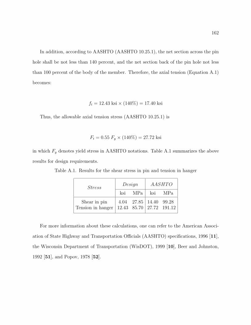
162

In addition, according to AASHTO (AASHTO 10.25.1), the net section across the pin

hole shall be not less than 140 percent, and the net section back of the pin hole not less

than 100 percent of the body of the member. Therefore, the axial tension (Equation A.1)

becomes:

ft = 12.43 ksi× (140%) = 17.40 ksi

Thus, the allowable axial tension stress (AASHTO 10.25.1) is

Ft = 0.55 Fy × (140%) = 27.72 ksi

in which Fy denotes yield stress in AASHTO notations. Table A.1 summarizes the above

results for design requirements.

Table A.1. Results for the shear stress in pin and tension in hanger

StressDesign AASHTO

ksi MPa ksi MPa

Shear in pin 4.04 27.85 14.40 99.28Tension in hanger 12.43 85.70 27.72 191.12

For more information about these calculations, one can refer to the American Associ-

ation of State Highway and Transportation Officials (AASHTO) specifications, 1996 [11],

the Wisconsin Department of Transportation (WisDOT), 1999 [10], Beer and Johnston,

1992 [51], and Popov, 1978 [52].

163

APPENDIX B

Material selection

The selection of materials may be driven by project requirements. For many decades,

bridges have been fabricated from plain carbon steels that have yield strengths between

36 ksi and 50 ksi.

Another problem with steel as a structural material is its susceptibility to corrosion.

Pre-heating and post-heating of these steels were generally needed to prevent welding

cracks that in combination with low fracture toughness (KC) of the steel at low temper-

ature have led to catastrophic failures [39].

B.1. NUCu 70W

In the early 1990s, the Federal Highway Administration (FHWA) and the Navy iden-

tified a need for a high performance weatherable structural steel that would have a 70 ksi

yield strength. Lower carbon content for improved welding and high fracture tough-

ness at cryogenic temperatures was desired for this steel. Under the auspice of the

FHWA/Navy/AISI Steering Committee a new steel designated ASTM HPS 70W was

developed. At Northwestern University, several years after the development described

above began, a different approach was taken to meet the 70 ksi yield strength target. A

NUCu 70W was thus created. The steel has a number of advantages over the ASTM HPS

70W. Under the Infrastructure Technology Institute (ITI) sponsorship, Fine and Vaynman

(2003) [53] developed a copper precipitation-hardened, high-performance weathering steel

164

(NUCu 70W) steel having the lowest carbon equivalent of any structural steel and can

be easily welded without pre- or post-heating. The fracture toughness is high compared

to other structural steels particularly at cryogenic temperatures. Weathering resistance

and corrosion resistance properties are better than those of any other available weather-

ing steel. Copper significantly improves the corrosion resistance of steel in marine and

inland environments. The high copper content in NUCu steel is effective in substantially

reducing the weight loss.

NUCu steel is now included in the ASTM A710 Standard. The steel was used for

rehabilitation of a bridge in Illinois. The Illinois Department of Transportation (IDOT)

recently announced the completion of a new bridge in Lake Villa, Lake County (Illinois)

constructed with NUCu steel.

Details can be found in Fine and Vaynman (2003) [53].

Table B.1. Material properties (NUCu 70W)

MaterialσY σUTS Elongation

ksi MPa ksi MPa %

NUCu 70W 70 483 80 552 27

B.2. ASTM A992

It should also be noted that the list of available steel changes from time to time. For

example, in the earlier to mid 1900s the only steel specification was ASTM A6 steel which

is no longer on the list [54].

Later other steels were developed including ASTM A36 and ASTM A572 which were

widely used in the building and bridge structures. A36 steel has a minimum yield stress

165

of 36 ksi. The ultimate tensile stress of this steel varies from 58 to 80 ksi. For design

calculations, it is suggested to use the minimum value of 58 ksi for the ultimate tensile

strength. Around the year 2000, ASTM A992 steel was introduced which meets the

requirements of both ASTM A36 and ASTM A572 and has now become the dominate

steel specification. ASTM A992 includes a yield strength range of 50 ksi to 65 ksi and a

minimum tensile strength of 65 ksi.

Details can be found in Zoruba and Grubb (2003) [54] and the SCM steel Construction

Manual (2003) [55].

166

APPENDIX C

Pack-rust formation and expansion

C.1. Introduction

In this Section, we present a simplified model describing the ratio of pack-rust expan-

sion based on chemical reaction.

As mentioned earlier, the failures in joint connections appear to be due to rust and

other corrosion products, which had built-up between the connecting devices over many

years. Figure C.1 illustrates the typical locations where corrosion is likely to occur.

For steel structures, such as bridges, the severity of deterioration will depend on how

long the metal is exposed to water, oxygen, and salt. The rate of corrosion in different

environments has been evaluated in several studies, in particular by Larrabee (1953) [56],

Legault et al. (1974) [57], Townsend et al. (1982) [58], and Coburn et al. (1995) [59].

Based on their studies, the rate of corrosion can accelerate significantly in the presence

of a marine environment or in cold regions where water and salt are usually combined.

C.2. Corrosion expansion calculation

Depending on the zone of attack, corrosion can occur as volume corrosion (three-

dimensional), surface corrosion (two-dimensional), line corrosion (one-dimensional), or

pitting (zero-dimensional). Further details on corrosion engineering can be found in text-

books, such as Uhlig (1948) [60] and Fontana (1986) [61].

167

Pack rust

(bottom pin)

Hanger

Pin

PinPin

Pin

Figure C.1. Typical pack rust formation

C.2.1. Chemical reaction

The corrosion of steel can be considered as an electrochemical process that occurs in

stages. Moist air and water containing carbon dioxide attack iron (Fe) to form rust that

is iron oxide hydrate (red rust), as schematically illustrated in Figure C.2. The sum of

these reactions can be represented by the following equation:

168

O2.Oads + 2Fe + 3H2O −→ Fe2O3.3H2O

Oxygen + Steel + Water −→ iron oxide hydrate (rust)

O H O

Iron (Fe)

22

Rust(iron oxyde hydrate)

Figure C.2. Schematic representation of the corrosion formation

The process requires the simultaneous presence of water (H2O) and oxygen (O2). In

the absence of either one, corrosion does not occur.

Because the resulting oxide layer is soft and porous, the changes can be calculated as

follows.

• A mass of one mole of iron (Fe) = 2× 56 = 112 g

• A mass of one mole of iron oxide hydrate is Fe2O3.3H2O = 2 × 56 + 3 × 16 +

3(1× 2 + 16) = 214 g

Thus, one gram (1 g) of iron is given by

1 g (Fe) =214

112= 1.91

169

Using density expressions, the volumes of rust (Fe2O3.3H2O) and iron (Fe) can be ex-

pressed respectively as,

vrust =mrust

drust

=214

4.28= 50.0 cm3

viron =miron

diron

=112

7.87= 14.23 cm3

where v, m, and d denote volume, mass, and density respectively. Therefore, the volume

expansion of these substances is expressed as,

vrust

viron

=50

14.23= 3.5

The result indicates that the pack-rust expansion is 3.5. This value provides a useful

indication of likely corrosion expansion. However, because of variations in atmospheric

environments, corrosion rate data cannot be generalized. It is the “micro-climate” imme-

diately surrounding the bridge structure which determines corrosion rates (or expansion)

for practical purposes. Details can be found in Larrabee (1953) [56], Legault et al. (1974)

[57], Townsend et al. (1982) [58], and Coburn et al. (1995) [59].

Life Cycle Management of Steel Bridges Based on NDE and ...

Documents

Transcript of Life Cycle Management of Steel Bridges Based on NDE and ...