Life Cycle Costs for Alaska Bridges -...

Ala

ska

Dep

artm

ent o

f Tra

nsp

orta

tion

& P

ub

lic Fa

cilities

Ala

ska U

niv

ersity T

ran

sporta

tion

Cen

ter

Life Cycle Costs for Alaska Bridges

T2-08-18 INE/ AUTC 15.02

J. Leroy Hulsey, Ph.D., P.E., S.E. Associate Director of the Alaska University Transportation Center

Professor of Civil & Environmental Engineering

University of Alaska Fairbanks

Billy Connor(Chapter 6), P.E. Director of the Alaska University Transportation Center


Andrew Metzger, Ph.D., P.E. Assistant Professor of Civil & Environmental Engineering

University of Alaska Anchorage

Donald J. Pitts, Graduate Student Graduate Student

Civil & Environmental Engineering


January 2015

Alaska University Transportation Center

Duckering Building Room 245

P.O. Box 755900

Fairbanks, AK 99775-5900

Alaska Department of Transportation

Research, Development, and Technology

Transfer

2301 Peger Road


REPORT DOCUMENTATION PAGE

Form approved OMB No.

Public reporting for this collection of information is estimated to average 1 hour per response, including the time for reviewing instructions, searching existing data sources, gathering and

maintaining the data needed, and completing and reviewing the collection of information. Send comments regarding this burden estimate or any other aspect of this collection of information,

including suggestion for reducing this burden to Washington Headquarters Services, Directorate for Information Operations and Reports, 1215 Jefferson Davis Highway, Suite 1204, Arlington,

VA 22202-4302, and to the Office of Management and Budget, Paperwork Reduction Project (0704-1833), Washington, DC 20503

1. AGENCY USE ONLY (LEAVE BLANK)

T2-08-18

2. REPORT DATE

August 2014

3. REPORT TYPE AND DATES COVERED

Final Report 05/2009-07/2011

4. TITLE AND SUBTITLE

Life Cycle Costs for Alaska Bridges 5. FUNDING NUMBERS

AUTC: 207083 T2-08-18

6. AUTHOR(S)

J. Leroy Hulsey, Ph.D., P.E., S.E.

Billy Connor, P.E.

Andrew Metzger, Ph.D., P.E.

Donald J. Pitts, Graduate Student

7. PERFORMING ORGANIZATION NAME(S) AND ADDRESS(ES)

Alaska University Transportation Center


Duckering Building Room 245

P.O. Box 755900


8. PERFORMING ORGANIZATION REPORT

NUMBER

INE/AUTC 15.02

9. SPONSORING/MONITORING AGENCY NAME(S) AND ADDRESS(ES)

State of Alaska, Alaska Dept. of Transportation and Public Facilities

Research and Technology Transfer

2301 Peger Rd


10. SPONSORING/MONITORING AGENCY

REPORT NUMBER

T2-08-18

11. SUPPLENMENTARY NOTES

12a. DISTRIBUTION / AVAILABILITY STATEMENT

No restrictions

12b. DISTRIBUTION CODE

13. ABSTRACT (Maximum 200 words)

A study was implemented to assist the Alaska Department of Transportation and Public Facilities (ADOT&PF) with life cycle costs for

the Alaska Highway Bridge Inventory. The study consisted of two parts. Part 1 involved working with regional offices of ADOT&PF to

assemble bridge costs (initial, construction, maintenance and repair) for a sample of bridge types. Results were limited by available data

and format; therefore, it is recommended that ADOT&PF develop an available online simple Bridge Management archiving system.

Part 2 focused on identifying how a bridge scheduled for replacement deteriorated over time. Load tests were conducted to help assess

the bridge response of an aged structure. Noticeable and measurable differences in strain at the end of the bridge life for the structure

studied were found.

A service life cycle costing approach has advantages over a traditional life cycle cost approach. For example, a bridge has essentially

three lives; structural, functional and service. Structural life can be extended almost indefinitely with the right repairs. The service life

approach does not assume a life. Rather it used to estimate a life that provides the lowest life cycle cost. A service life approach allows

comparisons of alternatives for an infinite planning horizon.

14- KEYWORDS :

Steel Bridges (Pdybmmms), Service Life (Ess), Life Cycle Costing (Esdmc), Life Cycle Analysis

(Esdm), Nondestructive Tests (Gbh), Steel Bridges (Pdybmmms), Load Factor (Rkmgm), Bridge Members (Pdybb), Bridge Substructures (Pdybbf), Structural health Monitoring(Grs) and

Bridge Bearing (Pdybbfe)

15. NUMBER OF PAGES

16. PRICE CODE

N/A 17. SECURITY CLASSIFICATION OF

REPORT

Unclassified

18. SECURITY CLASSIFICATION

OF THIS PAGE

Unclassified

19. SECURITY CLASSIFICATION

OF ABSTRACT

Unclassified

20. LIMITATION OF ABSTRACT

N/A

NSN 7540-01-280-5500 STANDARD FORM 298 (Rev. 2-98)

Prescribed by ANSI Std. 239-18 298-1

53

Notice This document is disseminated under the sponsorship of the U.S. Department of Transportation in the interest of information exchange. The U.S. Government assumes no liability for the use of the information contained in this document.

The U.S. Government does not endorse products or manufacturers. Trademarks or manufacturers’ names appear in this report only because they are considered essential to the objective of the document.

Quality Assurance Statement The Federal Highway Administration (FHWA) provides high-quality information to serve Government, industry, and the public in a manner that promotes public understanding. Standards and policies are used to ensure and maximize the quality, objectivity, utility, and integrity of its information. FHWA periodically reviews quality issues and adjusts its programs and processes to ensure continuous quality improvement.

Author’s Disclaimer Opinions and conclusions expressed or implied in the report are those of the author. They are not necessarily those of the Alaska DOT&PF or funding agencies.

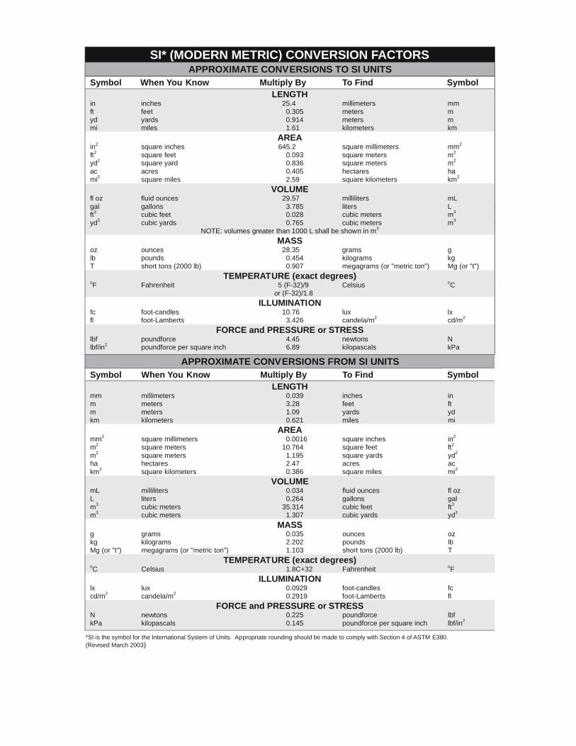
SI* (MODERN METRIC) CONVERSION FACTORS APPROXIMATE CONVERSIONS TO SI UNITS

Symbol When You Know Multiply By To Find Symbol LENGTH

in inches 25.4 millimeters mmft feet 0.305 meters myd yards 0.914 meters mmi miles 1.61 kilometers km

AREA in2 square inches 645.2 square millimeters mm2

ft2 square feet 0.093 square meters m2

yd2 square yard 0.836 square meters m2

ac acres 0.405 hectares ha mi2 square miles 2.59 square kilometers km2

VOLUME fl oz fluid ounces 29.57 milliliters mL gal gallons 3.785 liters Lft3 cubic feet 0.028 cubic meters m3

yd3 cubic yards 0.765 cubic meters m3

NOTE: volumes greater than 1000 L shall be shown in m3

MASS oz ounces 28.35 grams glb pounds 0.454 kilograms kgT short tons (2000 lb) 0.907 megagrams (or "metric ton") Mg (or "t")

TEMPERATURE (exact degrees) oF Fahrenheit 5 (F-32)/9 Celsius oC

or (F-32)/1.8 ILLUMINATION

fc foot-candles 10.76 lux lx fl foot-Lamberts 3.426 candela/m2 cd/m2

FORCE and PRESSURE or STRESS lbf poundforce 4.45 newtons N lbf/in2 poundforce per square inch 6.89 kilopascals kPa

APPROXIMATE CONVERSIONS FROM SI UNITS Symbol When You Know Multiply By To Find Symbol

LENGTHmm millimeters 0.039 inches inm meters 3.28 feet ftm meters 1.09 yards ydkm kilometers 0.621 miles mi

AREA mm2 square millimeters 0.0016 square inches in2

m2 square meters 10.764 square feet ft2

m2 square meters 1.195 square yards yd2

ha hectares 2.47 acres ackm2 square kilometers 0.386 square miles mi2

VOLUME mL milliliters 0.034 fluid ounces fl oz L liters 0.264 gallons galm3 cubic meters 35.314 cubic feet ft3

m3 cubic meters 1.307 cubic yards yd3

MASS g grams 0.035 ounces ozkg kilograms 2.202 pounds lbMg (or "t") megagrams (or "metric ton") 1.103 short tons (2000 lb) T

TEMPERATURE (exact degrees) oC Celsius 1.8C+32 Fahrenheit oF

ILLUMINATION lx lux 0.0929 foot-candles fc cd/m2 candela/m2 0.2919 foot-Lamberts fl

FORCE and PRESSURE or STRESS N newtons 0.225 poundforce lbfkPa kilopascals 0.145 poundforce per square inch lbf/in2

*SI is the symbol for th International System of Units. Appropriate rounding should be made to comply with Section 4 of ASTM E380. e(Revised March 2003)

i

TABLE OF CONTENTS

List of Figures ................................................................................................................................ iii

List of Tables ................................................................................................................................. iii

Executive Summary .........................................................................................................................1

Introduction ..............................................................................................................................3

1.1 General ..............................................................................................................................3

1.2 Overview and Scope of Work ...........................................................................................5

1.3 CR5000 Data Monitoring System .....................................................................................5

1.4 Instrumentation..................................................................................................................6

Literature Review .....................................................................................................................8

Noyes Slough Bridge, Part 1 ..................................................................................................11

3.1 General Information ........................................................................................................11

3.2 Construction/Planning .....................................................................................................11

3.3 Instruments (Types/Configurations) ...............................................................................13

3.3.1 Instrumentation Details ............................................................................................14

3.3.2 Thermistors ..............................................................................................................16

3.3.3 Strain Gauges ...........................................................................................................17

3.3.4 Accelerometers ........................................................................................................18

3.4 Programming (Campbell Scientific/Methods/Code) .......................................................19

Noyes Slough Bridge, part 2 ..................................................................................................21

4.1 Testing (Dump Truck) .....................................................................................................21

4.2 SAP2000 Model ..............................................................................................................23

ADOT&PF Bridge Cost Data .................................................................................................25

5.1 Original Maintenance Data .............................................................................................25

5.2 Results of Statistical Analysis .........................................................................................25

5.3 Construction Cost Situation ............................................................................................33

Estimating the Life Cycle Cost...............................................................................................35

Comparative Response (Structural deterioration) ..................................................................39

7.1 Comparison .....................................................................................................................39

7.2 Maintenance Data Compared with Noyes Slough Bridge ..............................................43

7.3 Importance of Construction Cost ....................................................................................44

ii

Conclusions ............................................................................................................................45

References ......................................................................................................................................46

iii

LIST OF FIGURES

Figure 1.1 Side view of the Noyes Slough Bridge.......................................................................... 4

Figure 1.2 Westbound view of Noyes Slough Bridge .................................................................... 4

Figure 1.4 Campbell Scientific CR5000 data acquisition system................................................... 6

Figure 1.5 Rolling platform and data collection staging area ......................................................... 7

Figure 3.1 Plan view of Bridge #0283, Noyes Slough Bridge...................................................... 11

Figure 3.2 Elevation view of Bridge #0283, Noyes Slough Bridge ............................................. 12

Figure 3.3 Bridge #0283, cross section of the steel girder superstructure .................................... 12

Figure 3.4 Hanging rolling platform ............................................................................................. 13

Figure 3.5 Wiring diagram for a YSI 44033 ................................................................................. 16

Figure 3.6 Thermistors before the final insulation application ..................................................... 16

Figure 3.7 Electrical diagram of a Wheatstone bridge ................................................................. 18

Figure 3.8 Wiring diagram of a single axial accelerometer .......................................................... 18

Figure 4.1 International 7600i day cab tipper ............................................................................... 21

Figure 4.2 SAP2000 model of the Noyes Slough Bridge ............................................................. 24

Figure 5.1 Total expenditure by fiscal year .................................................................................. 25

Figure 5.2 Average expenditure per type of bridge ...................................................................... 26

Figure 5.3 Percent of bridges maintained ..................................................................................... 27

Figure 5.4 Average total expenditures per type of maintained bridges ........................................ 28

Figure 5.5 Expenditures by type per year ..................................................................................... 28

Figure 5.6 Percent of expenditures by type per year of maintained bridges ................................. 29

Figure 5.7 Average expenditure by type per year of maintained bridges ..................................... 30

Figure 5.8 Average percent of expenditures by type per year of maintained bridges .................. 31

Figure 5.9 Stringer expenditures by age ....................................................................................... 32

Figure 5.10 Tee Beam expenditures by age .................................................................................. 32

Figure 5.11 Truss-Thru expenditures by age ................................................................................ 33

Figure 6.1 Minimum service life for a bridge structure ................................................................ 36

Figure 7.1 Strain test results comparison in End Span Beam #2 .................................................. 40

Figure 7.2 Strain test results comparison in End Span Beam #3 .................................................. 40

Figure 7.3 Strain test results comparison in Mid Span Beam #2 .................................................. 41

Figure 7.4 Changes in stress comparison in End Span Beam #2 .................................................. 41

Figure 7.5 Changes in stress comparison in End Span Beam #3 .................................................. 42

Figure 7.6 Changes in stress comparison in Mid Span Beam #2.................................................. 42

LIST OF TABLES

Table 3.1 Sensor installation documentation ................................................................................ 15

Table 7.1 Summary of costs for Alaska bridge types ................................................................... 44

1

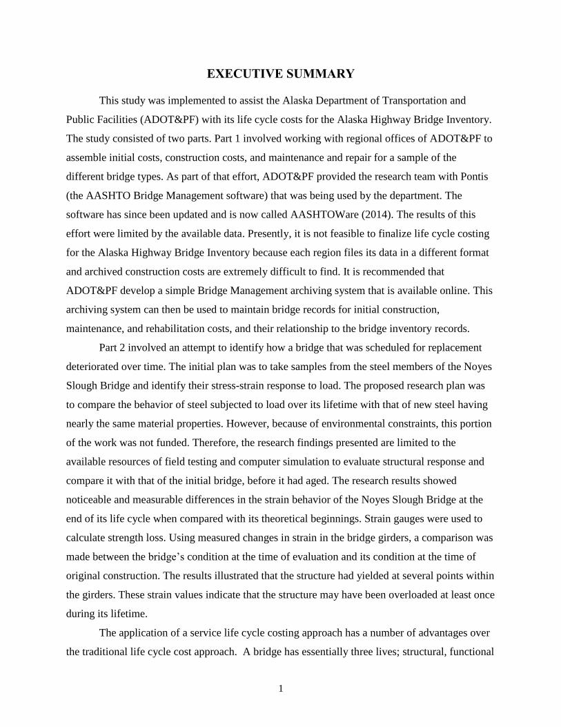
EXECUTIVE SUMMARY

This study was implemented to assist the Alaska Department of Transportation and

Public Facilities (ADOT&PF) with its life cycle costs for the Alaska Highway Bridge Inventory.

The study consisted of two parts. Part 1 involved working with regional offices of ADOT&PF to

assemble initial costs, construction costs, and maintenance and repair for a sample of the

different bridge types. As part of that effort, ADOT&PF provided the research team with Pontis

(the AASHTO Bridge Management software) that was being used by the department. The

software has since been updated and is now called AASHTOWare (2014). The results of this

effort were limited by the available data. Presently, it is not feasible to finalize life cycle costing

for the Alaska Highway Bridge Inventory because each region files its data in a different format

and archived construction costs are extremely difficult to find. It is recommended that

ADOT&PF develop a simple Bridge Management archiving system that is available online. This

archiving system can then be used to maintain bridge records for initial construction,

maintenance, and rehabilitation costs, and their relationship to the bridge inventory records.

Part 2 involved an attempt to identify how a bridge that was scheduled for replacement

deteriorated over time. The initial plan was to take samples from the steel members of the Noyes

Slough Bridge and identify their stress-strain response to load. The proposed research plan was

to compare the behavior of steel subjected to load over its lifetime with that of new steel having

nearly the same material properties. However, because of environmental constraints, this portion

of the work was not funded. Therefore, the research findings presented are limited to the

available resources of field testing and computer simulation to evaluate structural response and

compare it with that of the initial bridge, before it had aged. The research results showed

noticeable and measurable differences in the strain behavior of the Noyes Slough Bridge at the

end of its life cycle when compared with its theoretical beginnings. Strain gauges were used to

calculate strength loss. Using measured changes in strain in the bridge girders, a comparison was

made between the bridge’s condition at the time of evaluation and its condition at the time of

original construction. The results illustrated that the structure had yielded at several points within

the girders. These strain values indicate that the structure may have been overloaded at least once

during its lifetime.

The application of a service life cycle costing approach has a number of advantages over

the traditional life cycle cost approach. A bridge has essentially three lives; structural, functional

2

and service. All of these lives are highly variable. For example the structural life of a bridge can

be extended almost indefinitely with the right repairs. The service life approach does not assume

a life. Rather it estimates the life that provides the lowest life cycle cost. Doing so allows

comparisons of alternatives assuming an infinite planning horizon.

3

INTRODUCTION

1.1 General

The life of a bridge can be defined in multiple ways; structural, functional and service

life. The most common of these is the structural life, which can be defined as the point at which

the cost of repairing the bridge due to a structural element becomes economically unattractive.

The structural life of a bridge is critical, because at some point the bridge requires repair, load

reduction, or replacement. At this point, the associated costs should be compared to select the

most cost-effective alternative.

The functional life of a bridge is reached when a bridge no longer serves the need of the

public because of increased traffic, vehicle loading, or other required functions. As with the

structural life, there are multiple alternatives that correct functional deficiencies, including

replacement and upgrading, or rerouting traffic. Again, each alternative can be analyzed to

ascertain which is the most cost-effective.

The service life of a bridge is defined as that which minimizes its life cycle costs. The

advantage of this approach is the ability to merge functional and structural costs into a single

analysis. The service life of a bridge can be determined by computing either present worth or

equivalent annual costs, including the initial cost, for each year until a minimum life cycle cost is

found. The service life of the bridge does not mean the bridge has reached either its structural or

functional life. Rather the service life is simply the point at which life cycle costs begin to

increase after being at a minimum. Ideally, actual cost data adjusted for inflation would be used

to establish service life for each structural type. Unfortunately, those data do not exist, which

leaves two options: develop anticipated costs based on anecdotal data or develop a process that

can be applied as data become available. After a consultation with ADOT&PF, it was decided

that the second option would be chosen. That process is presented in Chapter 3.

The Noyes Slough Bridge (#0283), in service for over 60 years, provides an excellent

example of the life cycle of a bridge. This three-span composite steel girder, 172-foot-long

bridge had a roadway width of 30 feet (Figure 1.1, and 1.2). A 5-foot-wide sidewalk was built on

either side of the bridge in 1951. The structure was designed for AASHTO H20-44 highway

loads. The steel girders met the ASTM A242-4b. The 7¼-inch-thick reinforced concrete deck

was designed for 3000 psi 28-day concrete compressive strength. In 1982, about 850 square feet

4

of deck surface (the deck was 3843 sq ft) was delaminated and overlaid with 1 inch of polymer

concrete.

Figure 1.1 Side view of the Noyes Slough Bridge

Figure 1.2 Westbound view of Noyes Slough Bridge

Recently, the Noyes Slough Bridge, located in Fairbanks, Alaska, near the intersection of

Illinois Street and College Road, was replaced. Six decades of traffic, as well as extreme thermal

expansion and contraction, had taken its toll on the bridge’s structural integrity. This research

5

provides an estimate of strength loss in the structural steel of the bridge, as well as the bridge’s

most economical life cycle.

1.2 Overview and Scope of Work

When the Noyes Slough Bridge was considered for demolition, a project to evaluate the

structure’s remaining life was envisioned. The steel would be reclaimed, and strength tests would

be conducted. The bridge’s strength loss over its service time and its structural life cycle would

be learned. Due to unforeseen situations and higher-priority projects, the bridge was not

demolished during the study period; thus, an alternate course of action was planned.

A SAP2000 model of the bridge was created for use in determining the deflections of the

bridge as though it were newly constructed. After the bridge was instrumented, the structure was

tested by driving and stopping on the bridge at predetermined locations. The test vehicle was a

fully loaded ADOT&PF International 7600i dump truck. The dump truck was parked at locations

to establish the highest shear forces and moments in the support girders. A CR5000 Campbell

Scientific data logger was used to record data from strategically placed thermistors,

accelerometers, and strain gauges. Deflections recorded for maximum shear and moment tests

were used to assess strength loss. Using this information, a theoretical life cycle was calculated.

It was proposed that construction and maintenance data for bridges in Alaska would be

gathered from ADOT&PF’s master archive list and used for cost comparison with other similar

standing highway bridges in the state.

In other words, the study was performed in three stages: (a) Evaluate the remaining life of

the Noyes Slough Bridge by experimentally determining its condition; (b) create a SAP2000

three-dimensional finite element model of the bridge and analyze the structure for loaded dump

trucks; and (c) based on ADOT&PF records, perform an economic analysis of highway bridges

throughout Alaska.

1.3 CR5000 Data Monitoring System

The programmed Campbell Scientific CR5000 data logger (see Figure 1.4) is a rugged,

high-performance data acquisition system with a built-in keyboard, graphics display, and

PCMCIA card slot. It combines 16-bit resolution with a maximum throughput of 5000

measurements per second, has multiple input channels, and can measure a large number of

sensors.

6

The integrated keyboard and display screen on the CR 5000 data logger allows the user to

program, manually initiate data transfers, and view data on-site during testing. The integrated

PCMCIA slot accepts memory cards up to 2 GB for stand-alone data collecting. The CR5000

includes a current excitation channel that allows a direct connection of PRTs or other sensors

that use current excitation.

A battery-backed SRAM and clock ensure that data, programs, and accurate time are

maintained while the data logger is disconnected from the main power source. The CR5000 can

be used to collect and store experimental data; it can control peripherals and has proven valuable

for cold weather applications.

Figure 1.4 Campbell Scientific CR5000 data acquisition system

1.4 Instrumentation

Installation of the sensors required a staging platform, so a rolling platform was designed

to roll underneath the girders using the flanges as a guide (see Figure 1.5). Each gauge was

programmed into the data logger and installed on the bridge. A 12V deep cycle car battery was

used as a power source, and data was recorded and stored every time a vehicle triggered the data

logger.

Using as-built bridge construction drawings provided from ADOT& PF, a three-

dimensional model was prepared in SAP2000. Using this computer model, the bridge response

7

was simulated and compared with experimental data collected from the bridge site where a

loaded dump truck was positioned at various locations on the bridge. These tests were used to

correlate bridge behavior in relation to expected behavior when the bridge was new.

Finally, research was conducted to evaluate maintenance and construction data that was

provided by ADOT&PF.

Figure 1.5 Rolling platform and data collection staging area

8

LITERATURE REVIEW

Of the approximately 600,000 bridges in the United States, 24% are considered

structurally deficient or functionally obsolete. This pattern continues when focusing on Alaska.

Of the state’s 1156 bridges, about 22% are considered in the same state of disrepair as bridges in

other states (Ahmad, 2011). Many of these bridges have to be repaired or replaced. The question

is, Which bridge type is the most economical? And another, How much money can be saved if

bridges are replaced with the longest lasting, lowest construction and maintenance cost bridge?

Low-cost sensors and data collection systems allow rapid collection of data that may

indicate bridge health including loss of strength. Such information can be the first step in

determining many previously unknown facets of bridges, namely an accurate life cycle, an

economical life cost, and the type of bridge that is most cost-effective (Kerley and Lwin, 2011;

Kendall, Keoleian, and Helfand, 2008; Hawk, 2003). Other associated life cost studies were

reported by (Zhang, et al, 2003, 2005 and 2008).

Similar economics studies have been done on Bascule bridges in Chicago, Illinois, where

the bridge life exceeded the customary 75-year life cycle (Krizek et al., 2003). Their study found

that

the useful life is defined as the period from the initial construction to the point where the

reconstruction cost is greater than the initial cost. Most of the Chicago bridges studied

have never been reconstructed and have had a useful life greater than 75 years, which is

commonly assumed to be bridge design life. The first Chicago-type Bascule, the Cortland

Street Bridge, is currently more than 102 years old, page 2.

Krizek et al. (2003) also determined that

the results of their brief study showed that (a) the achievable useful life of a bascule

bridge can be more than 100 years, (b) the total life cycle cost of a 100-year-old bascule

bridge can be less than five times its initial cost, and (c) timely [maintenance, repair, and

rehabilitation] actions can lower the total life cycle cost of the bridge, page 6.

Therefore, clearly there is sparse data or supporting evidence that shows these bridges are

capable of withstanding 75 years of service, even though many are being used long after their

expiration date. America’s infrastructure is aging, and sufficient data to help us understand

exactly what is happening to aging bridges is unavailable. Even though Alaska is younger due to

9

statehood being more recent in comparison with the rest of the United States, the situation of

having insufficient data is no different.

Consider that throughout the useful life of bridge structures, each bridge is subjected to

routine and periodic maintenance, occasional rehabilitation, and some replacement work. Some

parts of the bridge deteriorate faster than others, and in some cases, a structure can experience

overloads or crash loads caused by different types of traffic accidents. Therefore, bridges require

a number of expenditures for various activities during their useful life (Hawk, 2003).

For bridge structures, maintenance and rehabilitation may be a significant part of the

Bridge Life-Cycle Cost Analysis (BLCCA), which can be expressed by

LCC DC CC MC RC UC SV (1)

where

LCC = life cycle cost;

DC = design cost;

CC = construction cost;

MC = maintenance cost;

RC = rehabilitation cost;

UC = user cost, and

SV = salvage cost.

Typically, user costs for bridge structures are a small part of the costs. The majority of

these costs occur during traffic congestion, bridge maintenance, or bridge rehabilitation.

Mohammadi et al. (1995) illustrated that a single parameter may be used to quantify the bridge

decision-making process. In this study, three elements were combined in the BLCCA: (a) bridge

condition rating, (b) costs resulting from work on the bridge, and (c) bridge life expectancy.

Mohammadi et al. (1995) illustrated this as follows:

( , , )VI F r c t (2)

where

VI = bridge value index,

F = objective function,

r = condition rating,

c = costs, and

t = time or bridge service life expectancy

Life cycle costs have been used in the transportation field for some time; however,

disagreement remains as to which cost items should be included with a given analysis. Delay

10

costs, fuel costs, vehicle operating costs, etc., are at the heart of the controversy. Other non-

agency costs such as environmental factors, expected life, changes in traffic patterns, the

influence of overloaded vehicles, deterioration rates, are difficult to estimate. In summary,

bridge life expectancy is not well defined; bridge behavior will affect a bridge’s expected life

and can change with type of materials, climatic exposure, traffic loads, overloads, and vehicle

crashes with the bridge structure (Hawk, 2003).

This study examines expected costs for different bridge types in the state of Alaska and

the aged response of the Noyes Slough Bridge. Initially, an evaluation of the condition of the

structural steel bridge members was proposed, sampling and testing their response in relationship

to the response of a new steel member. This idea was abandoned because of the risks of handling

and the expense associated with containment of the lead paint on the existing steel members.

Therefore, the second part of this study was limited to evaluating the bridge girder response to a

heavy truck load in an effort to determine the overall condition and remaining life of the

structural elements.

11

NOYES SLOUGH BRIDGE, PART 1

3.1 General Information

The initial portion of the analysis of the Noyes Slough Bridge is based on experimental

results that were found by measuring strain, accelerations, and member temperature.

Measurements were taken using weldable strain gauges, accelerometers, and thermistors. The

intention with this approach was to provide a better understanding of how a small multispan

bridge in Alaska reacts to daily traffic loading. Data from the measurements would be useful in

determining aspects of the bridge’s characteristics, such as the life cycle of the major structural

carrying members or strength loss over time.

3.2 Construction/Planning

To fully examine how the Noyes Slough Bridge reacts to everyday traffic loading, one

end span and the mid span were instrumented. Due to budgetary limitations and accessibility of

the undercarriage, focus was on only two of the three spans. This bridge is theoretically

symmetrical, so the two end spans should act the same (see Figures 3.1, 3.2, and 3.3). The

concrete deck was constructed to act compositely with the steel girders, but each steel girder is

simply supported between bents. In 1951, the concrete deck was built with a 28-day concrete

compressive strength of 3000 psi. By 1982, approximately 22% of the deck was delaminated.

That same year, deck repair consisted of replacing reinforcing bars, installing polymer concrete

patches, and placing a 1-inch polymer modified concrete overlay on the bridge deck.

Figure 3.1 Plan view of Bridge #0283, Noyes Slough Bridge

12

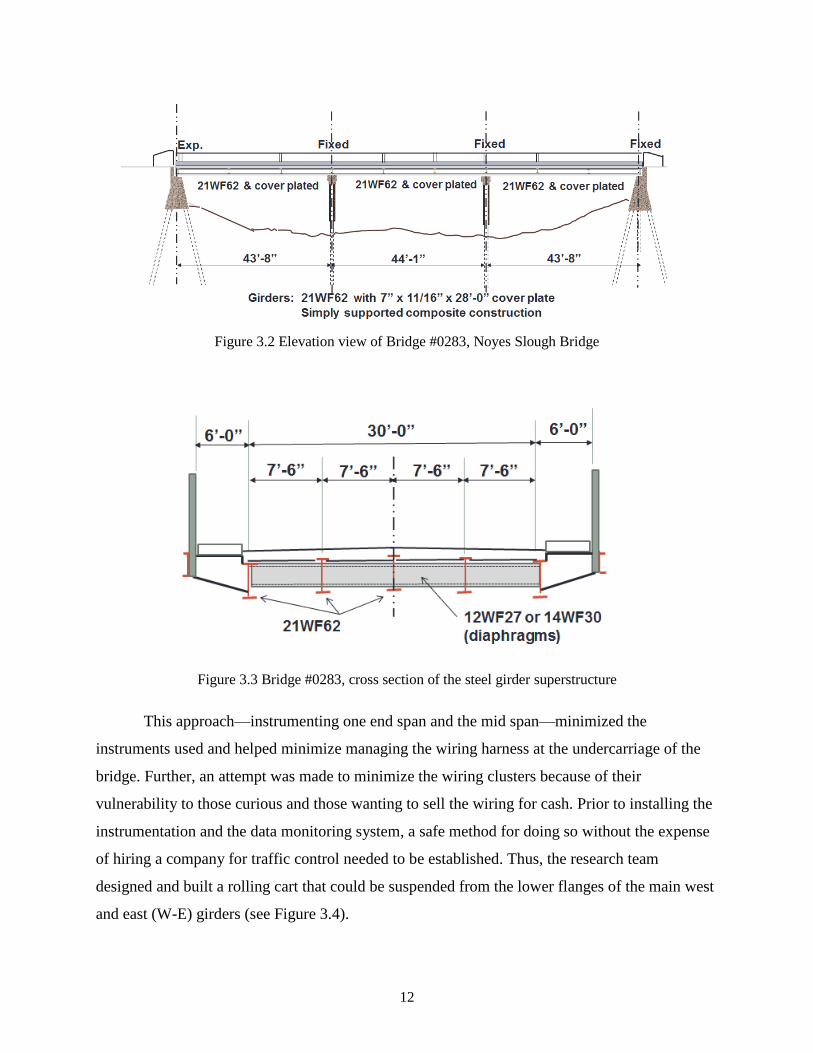
Figure 3.2 Elevation view of Bridge #0283, Noyes Slough Bridge

Figure 3.3 Bridge #0283, cross section of the steel girder superstructure

This approach—instrumenting one end span and the mid span—minimized the

instruments used and helped minimize managing the wiring harness at the undercarriage of the

bridge. Further, an attempt was made to minimize the wiring clusters because of their

vulnerability to those curious and those wanting to sell the wiring for cash. Prior to installing the

instrumentation and the data monitoring system, a safe method for doing so without the expense

of hiring a company for traffic control needed to be established. Thus, the research team

designed and built a rolling cart that could be suspended from the lower flanges of the main west

and east (W-E) girders (see Figure 3.4).

13

Figure 3.4 Hanging rolling platform

The movable instrumentation platform was designed to be lifted, installed, and moved by

only one person. When in use, the platform is approximately 15 to 20 feet above the ground. This

distance helped protect the onboard equipment from potential damage by the public. The

platform was designed and built so that it would roll along the bridge girders above the slough,

and so that one person could prepare and install the instrumentation at mid span. The platform

was built using two-by-fours with an OSB base. Four steel angles were attached at each corner.

Welded steel wheels and bearings were used to enable the platform to roll along the steel girder

flanges. To install the rolling platform, a chain link pulley system was designed and implemented

using modified S-hooks to anchor the chain at any place along its length, and steel C-clamps for

the chains to use as pulleys. Once the platform was completed and installed on the bridge, tools,

wires, and sensors could be applied to the bridge structure.

3.3 Instruments (Types/Configurations)

Three types of instruments were used to monitor the response of the Noyes Slough

Bridge: strain gauges, thermistors, and accelerometers. The sensors were monitored using a

Campbell Scientific Model CR000 data acquisition system. Continuous monitoring was

conducted by using a marine battery for power. Initially, the research team intended to

communicate with the equipment from the University of Alaska Fairbanks, but because of the

location of the bridge and the surrounding buildings and associated costs, that idea was

abandoned. Thus, the data were downloaded periodically and examined.

14

3.3.1 Instrumentation Details

All data was recorded by a Campbell Scientific CR5000 data logger with a AM16/32B

multiplexer. Twelve thermistors, four accelerometers, and sixteen strain gauges were installed on

the structure:

Twelve (12) Thermistors

Each was a YSI 55033, 2252 ohm resistor supplied by ThermX Southwest

Two (2) were used to measure ambient air temperature

Ten (10) were installed on the girder webs to measure temperature distribution

through the depth of the girder

Five (5) gauges were installed on two different girder webs to measure

temperature variation over depth. The gauges were placed evenly from top

to bottom of the web. The gauges were insulated to reflect the girder

temperature as accurately as possible.

Four (4) Accelerometers

One 20g uniaxial accelerometer was placed on top of the lower flange at mid span

on two different girders

One 20g triaxial accelerometer was placed on top of the lower flange at mid span

on two different girders

Sixteen (16) Strain Gauges

Each sensor was a five (5) volt 350 ohm full bridge weldable strain gauge

supplied by HITEC Products, Inc. (HPI)

Four gauges were placed at mid span on the top and bottom flanges of two

different girders to measure the girder flexural response to load

Two gauges were placed at the web centerline at the ends of two different girders

to measure girder shear

Summary

Sensors were only placed on one end span (span #1) and at mid span of span #2

All thermistors were placed on span #2

Two accelerometers were placed at mid span for span #1 and two at mid span for

span #2

Six strain gauges were placed at mid span of the first end span (span #1)

15

Six strain gauges were placed at mid span of span #2

Four strain gauges were placed at the web centerline located at the beginning of

the first span of the bridge (span #1)

Each sensor was assigned a unique five-digit label to help separate and describe them.

The first position ( X - - - ) is used to describe the sensor location (i.e., which of the two spans).

For example, “E” is end span and “M” is mid span. The second position ( - X - - ) is used to

determine which of the five girders the instrument is located on; that is, the girders are labeled

from 1 to 5 or South to North. Please note, only girders 2, 3, and 5 were instrumented. The third

position ( - - X - ) is used to denote the type of instrument; whether it is a strain gauge (S), a

single strain gauge of a pair used for shear (R), a thermistor (T), or an accelerometer (A). The

fourth position ( - - - X ) is used to designate the vertical position of the instrument; the highest

position is 1. Each location may have multiple instruments above or below it, designated by a 1

through 6, for instance, showing that there are 6 separate instruments near each other, one being

the highest relative position vertically to the others. A list of instruments and their positions is

shown in Table 3.1.

Table 3.1 Sensor installation documentation

Along bridge Girder Sensor Vertical position (1 to 6) Label

End span 2nd Strain x x E2S1-2

End span 3rd Strain x x E3S1-2

End span 5th Strain x x E5S1-2

Mid span 2nd Strain x x M2S1-2

Mid span 3rd Strain x x M3S1-2

Mid span 5th Strain x x M5S1-2

End span 3rd Shear strain x x E3R1-2

End span 3rd Accelerometer E3A1

End span 5th Accelerometer E5A1

Mid span 5th Accelerometer M5A1

End span 3rd Thermistors x x x x x x E3T1-6

End span 5th Thermistors x x x x x x E5T1-6

Examples: End span, 2nd girder strain gauges #1-2 (E2S1-2)

Mid span, 5th girder strain gauges #1-2 (M5S1-2)

End span, 5th girder strain gauges in shear #1-2 (E5R1-2)

End span, 3rd girder accelerometer (E3A1)

End span, 3rd girder thermistors #1-6 (E3T1-6)

16

3.3.2 Thermistors

The thermistors used in this study were a simple two-wire epoxy encapsulated YSI

44033. Created by ThermX, the thermistors are a standard 2252 ohms with an interchangeability

tolerance of ±0.1°C and a full operating temperature range of -80°C / +75°C (see Figures 3.5 and

3.6).

Figure 3.5 Wiring diagram for a YSI 44033

Figure 3.6 Thermistors before the final insulation application

A simple thermal resistor with metal sheathing for protection, the thermistors operate

within a 5V excitation, and record and convert resistance to temperature.

17

The thermistors were placed in a column of five along the web of two girders, just off

center of the end span of both the 3rd and 5th girders, fastened using weather stripping to insulate

them from the outside air. The weather stripping helped hold the instruments in place, while two

strips of shim stock steel were tack welded to permanently fasten the system in place (see Figure

3.6). Two thermistors were installed to hang from the girder so that an accurate ambient air

temperature could be obtained. Altogether, twelve thermistors were installed on the bridge

structure. Installation proceeded by first coating the steel and then insulating the thermistors with

a two-part expanding foam. The foam insulated the sensors from the outside air. This type of

application gives a more accurate representation of the actual temperature of the steel.

The placement of the thermistors provides information as to how the steel girders react to

the change in temperature as the day warms and cools. Throughout the day, every hour on the

hour, the thermistors were sent an excitation voltage so that the temperature could be recorded.

3.3.3 Strain Gauges

Girder strain was measured with full bridge amplified Wheatstone bridge weldable strain

gauges. These gauges were built and supplied by Hitec Products, Inc. (HPI). Classified as

HBWF-35-125-6-75UP-SS (x2) and HBWF-35-125-6-50UP-SS (x14), the only difference

between these two types of strain gauges is the length of the insulated cable; the former has 75

feet of UP cable, which is a four-conductor polyurethane (#22 AWG)-shielded jacket cable, and

the latter has 50 feet of cabling. It was determined that no discernable signal loss would occur

over the extra 25 feet of cabling.

The HPI strain gauges use Wheatstone bridge electrical circuits to ascertain the strain in

the girders on which they are attached (see Figure 3.7). The change in strain varies linearly with

the change in resistance. Resistance changes with the length change of the legs of the bridge

circuit. This change in resistance alters the outgoing measurable voltage.

18

Figure 3.7 Electrical diagram of a Wheatstone bridge

3.3.4 Accelerometers

Four accelerometers were used to instrument the Noyes Slough Bridge; three were

uniaxial in the z-axis (the direction of gravity), and one was triaxial. Accelerometers and strain

gauges behave similarly; only accelerometers use a piezoelectric crystal that alters the voltage as

it moves around, rather than a resistor stretched in a strain gauge (see Figure 3.8).

Figure 3.8 Wiring diagram of a single axial accelerometer

This voltage output is directly related to the force that is applied to the accelerometer.

The sensor voltages were recorded at a rate of 50 times per second (50 hertz). This measurement

provides an accurate view of how the bridge reacts to each vehicle that travels across it. The

19

acceleration data were used to signal the data logger to begin its collection cycle, rather than the

data logger constantly gathering data while the bridge is at rest. More about the collection cycle,

as well as how the accelerometers were used as triggers, is discussed in Section 3.5.

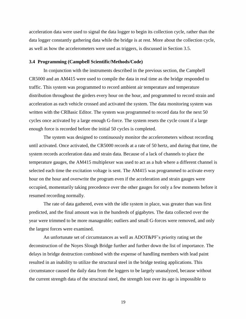
3.4 Programming (Campbell Scientific/Methods/Code)

In conjunction with the instruments described in the previous section, the Campbell

CR5000 and an AM415 were used to compile the data in real time as the bridge responded to

traffic. This system was programmed to record ambient air temperature and temperature

distribution throughout the girders every hour on the hour, and programmed to record strain and

acceleration as each vehicle crossed and activated the system. The data monitoring system was

written with the CRBasic Editor. The system was programmed to record data for the next 50

cycles once activated by a large enough G-force. The system resets the cycle count if a large

enough force is recorded before the initial 50 cycles is completed.

The system was designed to continuously monitor the accelerometers without recording

until activated. Once activated, the CR5000 records at a rate of 50 hertz, and during that time, the

system records acceleration data and strain data. Because of a lack of channels to place the

temperature gauges, the AM415 multiplexer was used to act as a hub where a different channel is

selected each time the excitation voltage is sent. The AM415 was programmed to activate every

hour on the hour and overwrite the program even if the acceleration and strain gauges were

occupied, momentarily taking precedence over the other gauges for only a few moments before it

resumed recording normally.

The rate of data gathered, even with the idle system in place, was greater than was first

predicted, and the final amount was in the hundreds of gigabytes. The data collected over the

year were trimmed to be more manageable; outliers and small G-forces were removed, and only

the largest forces were examined.

An unfortunate set of circumstances as well as ADOT&PF’s priority rating set the

deconstruction of the Noyes Slough Bridge further and further down the list of importance. The

delays in bridge destruction combined with the expense of handling members with lead paint

resulted in an inability to utilize the structural steel in the bridge testing applications. This

circumstance caused the daily data from the loggers to be largely unanalyzed, because without

the current strength data of the structural steel, the strength lost over its age is impossible to

20

establish with just the bridge’s daily reaction data. Therefore, an alternate form of analysis was

implemented and used to find the bridge’s strength loss.

21

NOYES SLOUGH BRIDGE, PART 2

This section of the Noyes Slough Bridge analysis provides the reader with a measure of

strength loss over the life of the bridge. The measure is based on evaluation without testing the

steel in a laboratory setting. Due to the constraints on ADOT&PF’s project workload, the bridge

remained in use a year longer than was expected, and structural health traffic monitoring was

conducted during the life of the structure. The strength loss was evaluated by calculating the

strain and deflection of the steel girders caused by test loads that were measured in preselected

positions on the structure. Calculated values were compared with the experimental data.

4.1 Testing (Dump Truck)

An International 7600i 6x4 day cab tipper was used to load the bridge structure with

known loads at known positions. These known truckloads were also used to test the monitoring

equipment (see Figure 4.1). Subsequently, the loaded truck was stopped at different locations to

measure static response for maximum moments and maximum shears. The dynamic response of

the bridge was measured by requesting the driver to drive across the bridge at a maximum safe

speed. Tests were conducted by having the driver drive in both directions across the bridge.

Figure 4.1 International 7600i day cab tipper

Thirty-six static load tests were used to determine the highest possible shear stress and

deflection on the two spans that were instrumented—the mid span and the west end span—as

well as six dynamic loads where the dump truck reached speeds upwards of 30 mph. These tests

were organized in a fashion that minimized the amount of time the truck was parked on the

22

bridge while the flaggers stopped traffic, and so that only a minimum number of truck turnabouts

were needed.

The first deflection test was conducted by having the truck driver position the front axle

at the middle of the west end span. For the next test, the driver positioned the truck so that the

next axle was positioned over the same midpoint. The following test was conducted by

positioning the truck with the rear axle at the same place on the bridge. The first test was at the

farthest outside edge of the eastbound lane. The driver moved the truck forward and repeated the

process on the midpoint of the mid span. The next set of deflection tests was a repeat of the

process, but westbound and on the outside edge of the westbound lane. The following set of tests

repeated the last but differed in lane placement; this time both tests were repeated but the dump

truck was in the inside edge of the lane. Finally, to finish the deflection tests, the dump truck was

directed eastbound in the very center of the bridge. The truck was positioned the same as for the

westbound tests.

Six static shear tests were conducted next. For these tests, the driver turned the dump

truck around and placed the front axle on a paint mark that was placed on the bridge deck prior

to testing. This paint mark was located so that the center of the load was one girder depth

distance away from the pier. The painted placement for the wheel was located to produce the

largest shear stresses. This test was at the west end span of the bridge. Then the truck was turned

around and the process was repeated for the eastbound outside edge of the lane. Once again, the

procedure used in the previous tests was repeated, with the truck driven down the inside edge of

the lane. Finally, the truck was positioned for an additional set of tests to evaluate the maximum

girder shear. This set of tests corresponded to the truck stopping on painted marks with the truck

located in the centerline of the bridge.

The last set of tests was the dynamic test, where the driver accelerated the dump truck as

much as possible. Due to the bridge’s proximity to the nearby intersection, reaching speeds over

25 to 30 mph proved difficult. The truck once again followed the previous test pattern by

accelerating westbound while staying on the outside edge of the lane and then turning around to

repeat the process eastbound. Then, the dump truck driver repeated the previous two tests while

being as far to the inside of the lane as possible. In the last two dynamic tests, the dump truck

was driven along the bridge centerline eastbound and then westbound. The truck axles, wheel

spacing, and weight were measured prior to testing on the bridge.

23

4.2 SAP2000 Model

An analysis of the Noyes Slough Bridge was done using a structural finite element

analysis program called SAP2000 (2014). The finite element model of the bridge was employed

to analyze the way the bridge reacted not only to daily traffic, but also to static and dynamic field

tests that were conducted with a pre-weighed and pre-measured ADOT&PF dump truck. The

model showed the reaction of the bridge when new to different positions and speeds of the

loaded dump truck. The virtual three-dimensional computer model was created from the

specifications and as-built drawings for this bridge.

For the model, the bridge’s main frame was mapped out and placed using basic

frame/cable lines, which later were changed to W21x62 beams for the main E-W girders. The

sub N-S girders had C12x25 channels at both ends. The sub N-S girders directly over the two

piers were W12x26 beams, and the sub N-S girders between the piers were W14x30 beams.

Once the main structure was created, the driving surface was placed and fixed to the girders. The

driving surface was treated as a shell, or thick plate section property, and sectioned by using the

intersection of the girders as a reference point. Each section of the driving surface was divided

into 8 equal pieces about 45 inches square. Then, due to the concrete welded onto the girders,

each thick plate intersection had a node that corresponded to a node on the girder 14 inches

below it, that was connected by a 2-joint link. This link essentially fastened the driving surface to

the girder below it, so all forces and moments were fully transferred between those nodes.

Once the model was completed and preliminary testing of the system showed that the

model was reacting to simple loading properly, a loading schedule was set up to the

specifications and locations of the dump truck tests (see Figure 4.2).

24

Figure 4.2 SAP2000 model of the Noyes Slough Bridge

After the computer model was checked to make sure that the forces were moving through

the model correctly, the final forces in each location corresponding with the previously described

dump truck test were placed, and the model was analyzed. This analysis gave the stresses

throughout the model and showed how each member of the bridge reacted to the tests. Using the

finite element model, stresses were calculated from strains and evaluated for strength

comparison. This approach was used as the basis for determination of strength loss over the

Noyes Slough Bridge’s life cycle.

25

ADOT&PF BRIDGE COST DATA

5.1 Original Maintenance Data

The Pontis database provided by ADOT&PF was used to evaluate all maintenance data.

The data were analyzed for fiscal years 2005 to 2010. The data were categorized in an effort to

better understand the maintenance trends of Alaska’s bridges throughout their life cycle.

Additionally, the data were compared with ADOT&PF’s construction records to determine the

most economical types of bridges currently built. One aspect not covered in depth here is the

drastic changes in temperature in the northern region versus the more temperate climates of the

southeast region. However, discrepancies appear even in this aspect, since Valdez is under the

northern region’s jurisdiction. With these problems aside, the data have been collected and

analyzed to maximize the information available.

5.2 Results of Statistical Analysis

Some parameters are more influential than other parameters, such as spending per fiscal

year, current age of the bridge, and type of bridge. Maintenance cost data were sorted by

spending per fiscal year, as shown in Figure 5.1.

Figure 5.1 Total expenditure by fiscal year

$-

$0.2

$0.4

$0.6

$0.8

$1.0

$1.2

$1.4

$1.6

2005 2006 2007 2008 2009 2010

Millio

ns

Fiscal Year

Total Expenditure by Year

26

Bridges were sorted into the following 13 unique bridge types stored in the Pontis

database:

Arch Deck

Box Beam Multi

Box Beam Single

Culvert

Girder and Floor beam

Orthotropic

Slab

Stayed Girder

Stringer

Tee Beam

Truss-Deck

Truss-Thru

Misc.

The bridge types were counted and organized to show relative expenditure for each type.

Data were then averaged over the total number of bridges for each type. The total for each type is

in parentheses after the name type and summarized in Figure 5.2.

Figure 5.2 Average expenditure per type of bridge

$-

$10,000

$20,000

$30,000

$40,000

$50,000

$60,000

Bridge Type (#)

Average Total Expenditures per Type of Existing Bridges

27

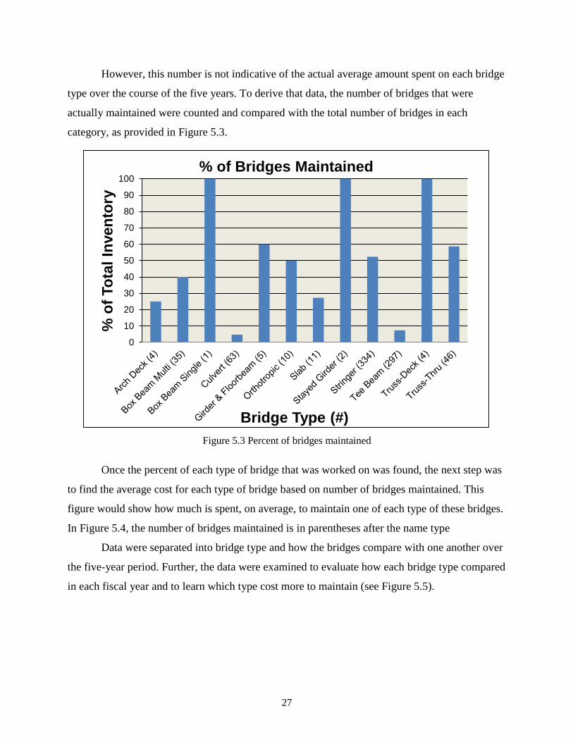
However, this number is not indicative of the actual average amount spent on each bridge

type over the course of the five years. To derive that data, the number of bridges that were

actually maintained were counted and compared with the total number of bridges in each

category, as provided in Figure 5.3.

Figure 5.3 Percent of bridges maintained

Once the percent of each type of bridge that was worked on was found, the next step was

to find the average cost for each type of bridge based on number of bridges maintained. This

figure would show how much is spent, on average, to maintain one of each type of these bridges.

In Figure 5.4, the number of bridges maintained is in parentheses after the name type

Data were separated into bridge type and how the bridges compare with one another over

the five-year period. Further, the data were examined to evaluate how each bridge type compared

in each fiscal year and to learn which type cost more to maintain (see Figure 5.5).

0

10

20

30

40

50

60

70

80

90

100

% o

f To

tal

Inven

tory

Bridge Type (#)

% of Bridges Maintained

28

Figure 5.4 Average total expenditures per type of maintained bridges

Figure 5.5 Expenditures by type per year

$-

$10,000

$20,000

$30,000

$40,000

$50,000

$60,000

$70,000

Bridge Type (Amount)

Average Total Expenditures per Type of Maintained Bridges

$-

$0.5

$1.0

$1.5

2005 2006 2007 2008 2009 2010

Millio

ns

Fiscal Year

Expenditures by Type per Year of Maintained Bridges

Misc

Truss-Thru

Truss-Deck

Tee Beam

Stringer

Stayed Girder

Slab

Orthotropic

Girder & Floorbeam

Culvert

Box Beam Single

Box Beam Multi

Arch Deck

29

Annual expenditures for maintenance were compared by bridge type. The comparison

was made by evaluating the percentage of total maintenance costs for bridges in Alaska. Figure

5.6 shows that most of each year’s expenditures were made on Tee Beams and Stringers, which

is due to there being more bridges in those two categories.

Figure 5.6 Percent of expenditures by type per year of maintained bridges

To provide a better understanding of how much it costs to maintain a given type of

bridge, it is helpful to examine the average cost by bridge type as compared with the entire

bridge population. The average expenditure per bridge when compared with its total population

is shown in Figure 5.7.

0%

10%

20%

30%

40%

50%

60%

70%

80%

90%

100%

2005 2006 2007 2008 2009 2010

Fiscal Year

% of Expenditures by Type per Year of Maintained Bridges

Misc

Truss-Thru

Truss-Deck

Tee Beam

Stringer

Stayed Girder

Slab

Orthotropic

Girder &FloorbeamCulvert

Box BeamSingleBox Beam Multi

Arch Deck

30

Figure 5.7 Average expenditure by type per year of maintained bridges

Figure 5.7 shows that the cost of Tee Beam bridges is nearly half of the costs per year,

not because of that population, but rather because the few that are maintained each year cost

quite a lot in comparison with other bridges like the steel Stringer.

The data from Figure 5.7 were divided into percentages for a clearer indication of the

average expenditure on each bridge type. This information is shown in Figure 5.8, which

presents how the expenditures are being divided per year and per bridge type.

$-

$20

$40

$60

$80

$100

2005 2006 2007 2008 2009 2010

Th

ou

san

ds

Fiscal Year

Average Expenditures by Type per Year of Maintained Bridges

Misc

Truss-Thru

Truss-Deck

Tee Beam

Stringer

Stayed Girder

Slab

Orthotropic


Box BeamSingleBox Beam Multi

31

Figure 5.8 Average percent of expenditures by type per year of maintained bridges

Another explored aspect of these bridge types is how the age of each bridge affects the

cost of its maintenance. Using Pontis database “yearbuilt” data, age was found and the data then

examined to show the differences in the amount spent on maintaining each type of bridge as it

aged. Figures 5.9, 5.10, and 5.11 show three examples of bridge types that had the highest

maintenance expenditures: Stringer, Tee Beam, and Truss-Thru.

In fact, a general trend shows that as a bridge ages it requires more and more

maintenance. This need is extremely clear in Figure 5.11, as many of the older bridges are

costing more to maintain. Note the large difference in age ranges of the Stringer bridge, 3 to 76

years, and the Tee Beam bridge, 4 to 49 years.

0%

10%

20%

30%

40%

50%

60%

70%

80%

90%

100%

2005 2006 2007 2008 2009 2010

Fiscal Year

Average % of Expenditures by Type per Year of Maintained Bridges

Misc

Truss-Thru

Truss-Deck

Tee Beam

Stringer

Stayed Girder

Slab

Orthotropic


Box BeamSingleBox BeamMulti

32

Figure 5.9 Stringer expenditures by age

Figure 5.10 Tee Beam expenditures by age

$0

$50,000

$100,000

$150,000

$200,000

$250,000

$300,000

3 14 18 20 23 26 28 30 33 36 38 40 42 44 46 49 51 53 55 57 59 61 71 76

Age (Years)

Stringer Expenditures by Age

$0

$50,000

$100,000

$150,000

$200,000

$250,000

4 6 8 12 14 17 19 21 23 25 27 29 31 33 35 37 44

Age (Years)

Tee Beam Expenditures by Age

33

Figure 5.11 Truss-Thru expenditures by age

5.3 Construction Cost Situation

After maintenance costs were determined and analyzed, the initial construction costs

were needed to find an accurate economic model. These records are held at each of the

corresponding regional office archives. Therefore, individual trips were required to gather the

appropriate information from each of the sites.

The Northern Region office of the ADOT&PF is organized differently than the other two

regional offices. The Northern Region office records are in hardcopy form and are filed in three-

ring binders in the master archive library, which makes finding initial construction costs quite

simple and intuitive. One simply checks the master archive list for the specific bridge or job. The

region’s master archive has a listing of whether the library contains information on anything

more than as-builts. If it does, then finding the binder is straightforward. If construction data are

there, the binder usually contains a final report along with a final accumulative change order.

The Central Region and Southeast Region ADOT&PF offices both use a different system

of data management. Due to the sheer quantity of records, a hardcopy of each record would

simply require too much space, so these two regions have opted to use microfiche for storing

records. This storage method is a great space saver, but it adds two more steps to finding

construction data: first finding as-builts and then finding the microfiche roll in the master list.

$0

$50,000

$100,000

$150,000

$200,000

$250,000

6 30 35 36 37 41 42 44 45 48 50 54 57 61 62 63 64 67 70

Age (Years)

Truss-Thru Expenditures by Age

34

Once these steps are taken, the data must be sifted through using projection readers—a rather

slow process and difficult to do for long periods.

It was not feasible to find the final construction costs for all of Alaska’s bridges due to

the time and effort needed for this task. A few small changes could be made by ADOT&PF that

would dramatically increase the feasibility of future economic analyses. Some of these changes

include but are not limited to the following:

organize databases according to final LPOs and final costs

cross-reference maintenance databases

organize final reports for each project

Currently, the information is simply too spread out for a full economic analysis to be

completed. Implementation of Bridge Life-Cycle Cost Analysis will not be practical until final

construction costs are organized in such a fashion as to facilitate that effort.

35

ESTIMATING THE LIFE CYCLE COST

There are multiple methods of determining the life cycle costs of bridges. The most

common method is to determine the present worth or equivalent annual cost of all expenditures

on the bridge throughout its life. This method is commonly found in engineering economy

textbooks. The difficulty is that the life of the structure must be assumed at the beginning. In

most life cycle cost determinations, the design life of the structure is used, knowing that,

generally, the expected life is considerably longer. As a result, the life cycle cost of the bridge

may be misleading.

A second method of estimating life cycle cost is using what is commonly called the

service life. In principle, the approach is quite straightforward. The present worth or equivalent

cost of the structure is computed for each life span beginning in year zero through the life, which

provides the lowest life cycle cost. Service life could be shorter or longer than the design life.

The service life does not directly assess the structural life, but simply estimates the life, which

minimizes the life cycle costs.

Consider the following example: The initial cost of a bridge is $2 million with a design

life of 75 years. The annual cost of maintenance is $3000 in Year 1 with an anticipated increase

in cost of 5% per year. The deck will require repaving every 15 years at a cost of $150,000. An

interest rate of 4% is assumed. Inflation will not be considered in this case. In determining

service life using the equivalent annual cost method, it is assumed that the reader has an

understanding of engineering economy.

The life cycle cost for Year 1 would be the (principle)(Capital Recovery Factor) plus the

maintenance costs in Year 1 or ($2 million)(1.04) + 1000 = $2,081,000.

Repeat this method for Year 2.

($2 million)(A/P,4,2) + [1000(1.0025)(P/F,4,2) + 1000)(A/P,4,2)]

= ($2 million)(.5302) + [1025(.9246) + 1000](.5302) = $1,061,432

Since the equivalent annual cost for Year 2 is less than for Year 1, compute the

equivalent annual cost for Year 3. Repeat these steps until a minimum is found.

This method lends itself very well to a spreadsheet, and Excel has financial functions

built in that easily allow these computations. The graph in Figure 6.1 shows a minimum life

cycle cost of about $109,873. For this example, those costs represent spending at the end of Year

69. Again, this value represents the economic service life of the structure and does not

36

necessarily relate to the structural or functional life. However, if costs during the life of the

structure can be anticipated, they can easily be incorporated into the analysis. For example, if it

is anticipated that an additional lane will be added in Year 50, the cost of the addition of that lane

can be incorporated into the analysis.

Figure 6.1 Minimum service life for a bridge structure

The advantage of the service life approach is that the analysis is not tied to a fixed life.

Rather, the economic life of each structure is estimated, and the associated cost of that structure

is estimated. Design alternatives are then compared based on this life cycle cost. As data become

available, the analysis can be tuned based on those data.

The challenge becomes the replacement strategy. Since bridge construction is a long-term

investment with no clear replacement requirement, it is assumed that the planning horizon is

infinite. Further, the service life does not necessarily represent optimal replacement timing. As

the structure ages, both structural and functional changes may occur. Consequently, the

assumptions made at the design stage may become invalid. A change to the structure or

37

replacement strategy may emerge, which then requires an analysis that determines how best to

address the new need.

The existing bridge, called the defender, will be compared with all alternatives, called the

challengers. Since the costs incurred to date are sunk costs, they cannot be considered in any of

the decision strategies. The steps listed below should be followed in selecting a replacement

strategy:

1. Compute the service life of both the defender and the challenger.

2. Compare the service lives. If the cost of the defender is higher than the cost of the

challenger, choose the challenger. If the cost of the challenger is higher than that of

the defender, choose the defender.

3. If the defender should not be replaced now, estimate when it should be replaced by

the challenger.

To demonstrate this process, two scenarios will be considered. The first scenario is

whether the bridge should be replaced in-kind in Year 71. The second scenario is whether to add

a lane to the existing bridge in Year 50 to accommodate traffic or to replace the bridge.

If in Year 71, the question is whether to replace the bridge or to replace the bridge in-

kind, the process is to look at the cost of maintaining the bridge for one more year and compare

that cost with the economic life of the new bridge. Since the bridge is being replaced in-kind, the

cost of maintaining the existing bridge one additional year must be less than the economic

service life of the new bridge, which is 69 years, with an equivalent annual cost of $109,873.

Looking at Figure 6.1 the estimated cost of maintaining the bridge in Year 70 is $86,993 plus a

capital cost of $150,000 for deck replacement. However, a deck inspection indicates the deck

does not need repairs for four years. Thus, the cost of routine repairs is less than $109,873. This

calculation suggests that the bridge be left in place for one more year. The process described is

continued until the costs exceed the economic life costs of the challenger. If only routine

maintenance is performed, the bridge would be replaced in Year 75 if the cost projected is

accurate. In truth, costs should be evaluated with current data rather than projected design data.

The second scenario essentially compares two alternatives. The first alternative is to

retrofit the bridge with an additional lane to accommodate traffic. The second alternative is to

build a new bridge to accommodate additional traffic. Both alternatives will occur in Year 50.

38

In this case, the service lives of the two alternatives are compared. Alternative 1 assumes

a retrofit cost of $1,000,000, which includes the cost of resurfacing the existing deck and some

modifications to reduce routine maintenance costs. Because the bridge has aged, the maintenance

costs will be higher than a new bridge at $15,000 per year at a growth rate of 5% per year. The

estimated cost of resurfacing the deck increases to $175,000 every 10 years. Using the same

procedure as before, the service life of the bridge after rehabilitation and widening is an

additional 47 years at an equivalent annual cost of $146,737.

Assume a new bridge can be constructed for $4 million with an initial maintenance cost

of $2000 per year with an annual growth rate of 3% due to new design technologies. It is

anticipated that the deck will be re-decked every 15 years at a cost of $225,000. In this case, the

service life is 81 years at an equivalent annual cost of $104,409. Replacing the bridge becomes

the most economically attractive decision.

As always, intrinsic values, including available funding, environmental impacts, and

community input, must be considered. In summary, the economic life approach offers a number

of advantages over traditional life cycle cost analysis for infrastructure that has a very long life.

The most attractive advantage is that the procedure does not require assigning an analysis life.

Rather, the procedure determines the life at which the life cycle costs are at a minimum. This

method allows ready comparison of multiple alternatives with long lives and an analysis of

modification of potential changes in strategy at any point in the life of the structure. While the

procedure is somewhat more complex, spreadsheets allow for rapid analysis. Once the

spreadsheet is set up, it can be rapidly altered to accommodate changes in assumptions or

modified for other alternatives.

39

COMPARATIVE RESPONSE (STRUCTURAL DETERIORATION)

7.1 Comparison

The research findings from this study show that there were noticeable and measurable

differences in the strain behavior of the Noyes Slough Bridge at the end of its life cycle when

compared with its theoretical beginnings. Strain gauges were used to calculate strength loss.

Using measured changes in strain in the bridge’s girders, a comparison was made between the

bridge’s condition at the time of evaluation and its condition at the time of original construction.

With this method, changes in stress could be quite easy to find.

Not every strain gauge responded as predicted. Many of the strain gauges showed signs

of change during the test, yet after analysis, these changes proved to be negligible. Therefore,

only strain gauges that showed changes in strain that paralleled the SAP2000 model were used

for the final analysis. Also, for the final analysis, only girders that experienced the greatest

amount of strain from the location of the dump truck were used for the most accurate picture of

strength loss.

Careful consideration of the data analysis indicated a clear trend of increasing strain, or

increasing stress, over the life of the structure. Figures 7.1, 7.2, and 7.3 show what the strain in

the beams should have been when the bridge was first built, as compared with the strain in the

beams during the test.

40

Figure 7.1 Strain test results comparison in End Span Beam #2

Figure 7.2 Strain test results comparison in End Span Beam #3

0

50

100

150

200

250

300

EBOE1 EBOE2 EBOE3 EBIE1 EBIE2 EBIE3 EBCE1 EBCE2 EBCE3

% S

trai

n In

crea

se

Various Tests (Name)

Percent of Strain Increase in End Span Beam #2 as Compared with SAP2000

Model

-50

50

150

250

350

EBO

E1

EBO

E2

EBO

E3

WB

OE1

WB

OE2

WB

OE3

EBIE

1

EBIE

2

EBIE

3

WB

IE1

WB

IE2

WB

IE3

EBC

E1

EBC

E2

EBC

E3% S

trai

n In

crea

se


Percent of Strain Increase in End Span Beam #3 as Compared with SAP2000

Model

41

Figure 7.3 Strain test results comparison in Mid Span Beam #2

In each of these cases, it can be seen conclusively that beam strains increased and, in

turn, their stress increased. In many cases, the increase was well over 100%. The stress values

associated with these increases are shown in Figures 7.4, 7.5, and 7.6.

Figure 7.4 Changes in stress comparison in End Span Beam #2

0100200300400500600700

% S

trai

n In

crea

se


Percent of Strain Increase in Mid Span Beam #2 as Compared with SAP2000

Model

0

20

40

60

80

100

EBOE1 EBOE2 EBOE3 EBIE1 EBIE2 EBIE3 EBCE1 EBCE2 EBCE3

Stre

ss (

ksi)


Increase in Stress Comparison from Initial Bridge as Constructed in End Span

Beam #2 Maximum state of stress

(yielded)

42

Figure 7.5 Changes in stress comparison in End Span Beam #3

Figure 7.6 Changes in stress comparison in Mid Span Beam #2

-40

-20

0

20

40

60

80

100

120St

ress

(ks

i)


Change in Stress Comparison from Tests vs. SAP2000 in End Span Beam #3

0

20

40

60

80

100

120

EBOM1 EBOM2 EBOM3 EBIM1 EBIM2 EBIM3 EBCM1 EBCM2 EBCM3

Stre

ss (

ksi)


Change in Stress Comparison from Tests vs. SAP2000 in Mid Span Beam #2

Maximum state of stress

(yielded)

Maximum state of stress

(yielded)

43

Nearly every test showed a marked increase in strain and stress in the beams when

compared with its SAP2000 theoretically calculated values based on the original (new)

construction condition. With an average stress increase of 43.35 ksi in End Span Beam #2, 27.60

ksi in End Span Beam #3, and 52.32 ksi in Mid Span Beam #2, it is easy to see a direct

correlation between the use of 62 years and the bridge’s theoretical beginnings. These stress

increases are based on the concept that stress is proportional to strain (linear behavior). Clearly,

in this case, parts of the structure may have experienced yield, and the member carrying capacity

may have been redistributed so that areas less stressed would contribute to the load-carrying

capacity of the structure. These stresses were calculated from the strains measured in the gauges;

therefore, assuming that the stress increases of these beams show the beams have undergone

yielding deformation is reasonable. The minimum yield strength of these beams was Fy = 36 ksi,

and the effective yield stress was Fye = 54 ksi. The effects of traffic and weather caused the

Noyes Slough Bridge beams to experience significant states of stress, and these effects led to the

redistribution of stress throughout the rest of the beam.

7.2 Maintenance Data Compared with Noyes Slough Bridge

The Noyes Slough Bridge is classified as a steel Stringer type with a reinforced concrete

deck, placing it in the largest category for bridge types in the state of Alaska. In 2013, Alaska

had 334 bridges with the classification of Stringer. This means that a lot of money was spent

maintaining these bridges; however, as noted in Chapter 5, Stringer bridges are some of the

cheapest to maintain per year, per bridge, making them a very efficient bridge type—little

maintenance cost and a long life span.

When Alaska achieved statehood in 1959, the Noyes Slough Bridge was already about

ten years old. The ADOT&PF was decentralized, and most of its records were transferred. The

original construction cost of the bridge has not been found; therefore, an accurate assessment of

its full life cycle is not possible. Prior to this study, the bridge was decommissioned after visual

inspections. During this study, the bridge was replaced. Construction of the new Noyes Slough

Bridge, located near the intersection of Illinois Street and College Road in Fairbanks, was part of

a street improvement project for Illinois Street.

44

7.3 Importance of Construction Cost

The initial construction costs of many bridges in Alaska are not available. Only 28 initial

construction costs from 5 different bridge types were found. Of those bridges, nearly all of them

were 40 years old, or younger, with the average being 35 years old. Only the most current

records on bridges are readily available from ADOT&PF. Table 7.1 shows the 5 types of bridges

that rank the most cost-effective by initial cost plus yearly maintenance over their life span:

Table 7.1 Summary of costs for Alaska bridge types

Bridge Type Initial Cost Plus Annual Maintenance Cost

Arch Deck $1,195,088

Box Beam $1,475,702

Tee Beam $4,443,132

Stringer $7,199,380

Orthotropic $36,812,406

The list provided in Table 7.1 is only a partial list of the bridge types in Alaska. In the

case of both the Arch Deck bridge and the Orthotropic bridge, only one entry was found. The

Noyes Slough Bridge falls under the category of Stringer bridges and, therefore, according to the

data, is one of the most expensive bridge types on this list. Without proper data and accurate

records, it is nearly impossible to analyze the work of so many engineers and contractors who

labored to create before us. Therefore, it is vital that a system, easily accessible and instantly

maintained by the ADOT&PF, be implemented. Pontis is the current software system in place at

ADOT&PF, and it has a long way to go before it can be considered a central system of data

access and storage throughout the department.

45

CONCLUSIONS

Throughout the course of this study, many insights were gained,into the way a bridge

reacts under live load, to the cost of maintaining bridges throughout the state of Alaska and how

the life cycle cost of bridges might be determined.

A clear loss of strength was found in the Noyes Slough Bridge; the structure exceeded

twice the strain it was designed for when new. All bridges throughout Alaska were cataloged and

then sorted by bridge type. The cost to maintain each bridge was determined, and the

maintenance costs were statistically analyzed. Initial construction costs were missing for many of

these bridges, including the Noyes Slough Bridge, so though its bridge type is one of the

cheapest to maintain, an accurate cost benefit analysis of the bridge was impossible.

The Noyes Slough Bridge was demolished in the summer of 2013, ending any further

data that could have been recorded from traffic usage over the girders. While replacing the

bridge was the ultimate plan, demolition occurred later than planned due to higher ADOT&PF

priorities. Essentially, with this study, much more is now known about the Noyes Slough Bridge

and its relationship to the rest of the bridges throughout Alaska.

The application of the service life cycle costing approach has a number of advantages

over the traditional life cycle cost approach. A bridge has essentially three lives; structural,

functional and service. All of these lives are highly variable. For example the structural life of a

bridge can be extended almost indefinitely with the right repairs. The service life approach does

not assume a life. Rather it estimates the life that provides the lowest life cycle cost. Doing so

allows comparisons of alternatives assuming an infinite planning horizon.

46

REFERENCES

AASHTOWare. 2014. Bridge Management Software (formerly Pontis).

Ahmad, A. 2011. “Bridge Preservation Guide.” FHWA-HIF-11042, FFHWA, August.

Hawk, H. 2003. “Bridge Life-Cycle Cost Analysis.” NCHRP Report 483, Transportation

Research Board, Project C12-43 FY 96, ISSN 0077-5614, ISBN 0-309-06801-0.

Kendall, A., G.A. Keoleian, and G.E. Helfand. 2008. “Integrated Life Cycle Assessment and

Life Cycle Cost Analysis Model for Concrete Bridge Deck Applications.” Journal of

Infrastructure Systems, ASCE, September.

Kerley, M.T., and M.M. Lwin. 2011. “Bridges: Life Cycle Costing.” National Steel Bridge

Alliance, Modern Steel Construction, June.

Krizek (et al.?) , 2003, Life Cycle Costs of Bridges, Final Report, Infrastructure Technology

Institute for TEA, Northwestern University.

Mohammadi, J., S.A. Guralnick, and L. Yan. 1995. “Incorporating Life-Cycle Costs in Highway-

Bridge Planning and Design.” ASCE Journal of Transportation Engineering, Vol. 121, Part

3. pp. 417–424.

SAP2000. 2014. Computers and Structures, Structures and Earthquake Engineering Software.

Zhang, Y., Novick, D.A, Hadavi, A. and Krizek, R.J., (2003), Part 1 - Whole Life Cycle Cost for

Chicago-Type Bascule Bridges, Infrastructure Technology Institute for TEA, Northwestern

University.

Zhang, Y., D. Novick, A. Hadavi, and R. Krizek. 2008. “Whole Life Cycle Cost for Chicago-

Type Bascule Bridges.” Cost Engineering, 50(4): p. 28, April.

Zhang, Y., Novick, D., Hadavi, A., and Krizek, R. (2005) Life-Cycle Cost Analysis of Bridges

and Tunnels. Construction Research Congress 2005: pp. 1-9.

Life Cycle Costs for Alaska Bridges -...

Documents

Transcript of Life Cycle Costs for Alaska Bridges -...