LIFE CYCLE COST AND ENVIRONMENTAL IMPACT …
11
HAL Id: hal-01722753 https://hal.archives-ouvertes.fr/hal-01722753 Submitted on 21 Apr 2020 HAL is a multi-disciplinary open access archive for the deposit and dissemination of sci- entific research documents, whether they are pub- lished or not. The documents may come from teaching and research institutions in France or abroad, or from public or private research centers. L’archive ouverte pluridisciplinaire HAL, est destinée au dépôt et à la diffusion de documents scientifiques de niveau recherche, publiés ou non, émanant des établissements d’enseignement et de recherche français ou étrangers, des laboratoires publics ou privés. LIFE CYCLE COST AND ENVIRONMENTAL IMPACT OPTIMIZATIONS OF A LOW VOLTAGE DRY TYPE DISTRIBUTION TRANSFORMER Benoît Delinchant, Guillaume Mandil, Frédéric Wurtz To cite this version: Benoît Delinchant, Guillaume Mandil, Frédéric Wurtz. LIFE CYCLE COST AND ENVIRONMEN- TAL IMPACT OPTIMIZATIONS OF A LOW VOLTAGE DRY TYPE DISTRIBUTION TRANS- FORMER. COMPEL: The International Journal for Computation and Mathematics in Electrical and Electronic Engineering, Emerald, 2018, 37 (2), pp.645-660. 10.1108/COMPEL-12-2016-0533. hal- 01722753
Transcript of LIFE CYCLE COST AND ENVIRONMENTAL IMPACT …

HAL Id: hal-01722753https://hal.archives-ouvertes.fr/hal-01722753
Submitted on 21 Apr 2020
HAL is a multi-disciplinary open accessarchive for the deposit and dissemination of sci-entific research documents, whether they are pub-lished or not. The documents may come fromteaching and research institutions in France orabroad, or from public or private research centers.
L’archive ouverte pluridisciplinaire HAL, estdestinée au dépôt et à la diffusion de documentsscientifiques de niveau recherche, publiés ou non,émanant des établissements d’enseignement et derecherche français ou étrangers, des laboratoirespublics ou privés.
LIFE CYCLE COST AND ENVIRONMENTALIMPACT OPTIMIZATIONS OF A LOW VOLTAGE
DRY TYPE DISTRIBUTION TRANSFORMERBenoît Delinchant, Guillaume Mandil, Frédéric Wurtz
To cite this version:Benoît Delinchant, Guillaume Mandil, Frédéric Wurtz. LIFE CYCLE COST AND ENVIRONMEN-TAL IMPACT OPTIMIZATIONS OF A LOW VOLTAGE DRY TYPE DISTRIBUTION TRANS-FORMER. COMPEL: The International Journal for Computation and Mathematics in Electrical andElectronic Engineering, Emerald, 2018, 37 (2), pp.645-660. �10.1108/COMPEL-12-2016-0533�. �hal-01722753�

1
LIFE CYCLE COST AND ENVIRONMENTAL IMPACT OPTIMIZATIONS
OF A LOW VOLTAGE DRY TYPE DISTRIBUTION TRANSFORMER
Benoit Delinchant*, Guillaume Mandil**, Frédéric Wurtz*
* Univ. Grenoble Alpes, CNRS, G2Elab, F-38000 Grenoble, France
E-mail: [email protected]
** Univ. Grenoble Alpes, CNRS, G-SCOP, F-38000 Grenoble, France
Abstract. Life Cycle Analysis (LCA) is more and more used in the context of electromagnetic product
design. But it is often used to check a design solution regarding environmental impacts after technical and
economical choices. In this paper, we are investigating Life Cycle Impact Optimization (LCIO) and comparing
with the classical Life Cycle Cost Optimization (LCCO). First, a model of a dry type transformer using different
material for windings and magnetic core is presented. LCCO, which is a mixed continuous-discrete, multi-
objective technico-economic optimization, is done using both deterministic and genetic algorithms. LCCO
results and optimization performances are analysed, and a LCA is presented for a set of optimal solutions. The
final part is dedicated to the LCIO, where we are showing that these optimal solutions are very close to those
obtained with LCCO.
Keywords. life cycle analysis, life cycle costs, multi-objective optimization.
INTRODUCTION
This paper is about multi-objective optimization for the design of electrical devices that have financial
and environmental impacts during both the manufacturing process and their usage. Indeed, the production phase
of an electrical engineering product requires the use of expensive materials and could impact the depletion of
natural resources. In addition, the use of electrical equipment that has a low efficiency, leads to excessive energy
consumption, which corresponds to high financial costs, but also significant impacts on environment such as
global warming effect. In this work we are studying more deeply the case of a low voltage dry type distribution
transformer.
Studies on the life cycle analysis of transformers have already been conducted. In [1], a bi-objective
optimization of the active mass of the transformer and the global life cycle energy cost is performed and classical
Pareto front is used in order to help designer to choose his preferred solution. In [2], a model of environmental
impacts is used jointly with economic and electromagnetic models in a multi-objective optimization to find the
best trade-off between those criteria. In these previous works we can see the increase of criteria that have to be
optimized. First of all, it requires the ability to express the calculation of these objectives in a single model. This
can be achieved by combining models together (physical, economical, environmental), which require to adapt
models or to use interoperability solutions [10]. Computer Aided Design tools may provide the right information
in order to help the designer in an efficient manner. In this work, we will show that addressing financial costs or
environmental impacts may lead to the same design solution.
MODELING A LOW VOLTAGE DRY TYPE DISTRIBUTION TRANSFORMER
According to the International Copper Association (Table 1), it is possible to save a lot of energy, carbon dioxide
emissions, and dollars, by replacing distribution transformers with more efficient ones. 3 scenarii are studied
from a basic one (1) to the most improved (3) and compared to the current scenario. This study could be done for
all electrical devices, but it is a lot of work. Here we are trying to bring to designer the information that will help
him to choose the best design according to its own vision of financial, energy, and environment aspects.

Table 1. Projected annual global savings potential compared to the historic base-case scenario [The International Copper Association, Global energy savings from high efficiency distribution transformers,
White Paper, By Hans De Keulenaer, Waide Strategic Efficiency Limited and N14 Energy Limited, 22/10/2014]
Years current scenario scenario 1 scenario 2 scenario 3
In this paper, we are dealing with a classical distribution transformer in which a Life Cycle Analysis
(LCA) including economic and environmental performances evaluation. In order to do this, a fist model is
required regarding the electromagnetic. Then an economic model and an environmental model, are based on
transformer material masses, and the energy consumption during its operation.
1. Electromagnetic Modelling
The electromagnetic model is based on a classical equivalent circuit approach (Figure 1).
Figure 1. Equivalent Circuit Model
Core loss resistance Ro is related to the grain-oriented electrical steel properties. In this work, we are
using two kind of magnetic material that have different performances (M2 and M6, Table 2) .
Table 2. Core losses in Watts per Kilogram at 50 Hz [ATI Allegheny Ludlum, Technical Data, Grain-Oriented Electrical Steel]
Magnetizing reactance Xm is related to the coil number of turn and magnetic circuit geometry (see
equation (1) and Figure 2. Magnetic circuit). It is calculated using reluctance approach and the worst reluctance is
used (), ie the one seen from a winding placed on an outside leg (left or right side).
𝑋𝑚 = 𝐿𝑚. 𝜔 =𝑁2
(1)
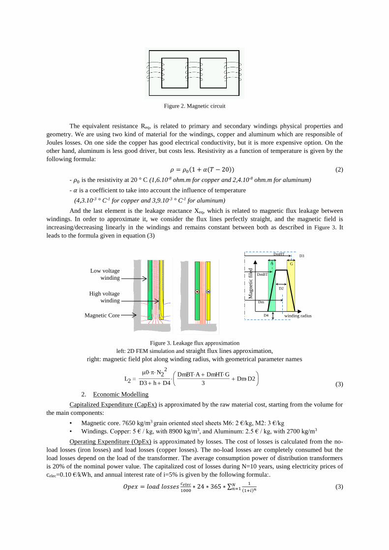
Figure 2. Magnetic circuit
The equivalent resistance Req, is related to primary and secondary windings physical properties and
geometry. We are using two kind of material for the windings, copper and aluminum which are responsible of
Joules losses. On one side the copper has good electrical conductivity, but it is more expensive option. On the
other hand, aluminum is less good driver, but costs less. Resistivity as a function of temperature is given by the
following formula:
𝜌 = 𝜌0(1 + 𝛼(𝑇 − 20)) (2)
- 𝜌0 is the resistivity at 20 ° C (1,6.10-8 ohm.m for copper and 2,4.10-8 ohm.m for aluminum)
- 𝛼 is a coefficient to take into account the influence of temperature
(4,3.10-3 ° C-1 for copper and 3,9.10-3 ° C-1 for aluminum)
And the last element is the leakage reactance Xeq, which is related to magnetic flux leakage between
windings. In order to approximate it, we consider the flux lines perfectly straight, and the magnetic field is
increasing/decreasing linearly in the windings and remains constant between both as described in Figure 3. It
leads to the formula given in equation (3)
Figure 3. Leakage flux approximation
left: 2D FEM simulation and straight flux lines approximation,
right: magnetic field plot along winding radius, with geometrical parameter names
L2
0 N22
D3 h D4
DmBT A DmHT G
3Dm D2
(3)
2. Economic Modelling
Capitalized Expenditure (CapEx) is approximated by the raw material cost, starting from the volume for
the main components:
• Magnetic core. 7650 kg/m3 grain oriented steel sheets M6: 2 €/kg, M2: 3 €/kg
• Windings. Copper: 5 € / kg, with 8900 kg/m3, and Aluminum: 2.5 € / kg, with 2700 kg/m3
Operating Expenditure (OpEx) is approximated by losses. The cost of losses is calculated from the no-
load losses (iron losses) and load losses (copper losses). The no-load losses are completely consumed but the
load losses depend on the load of the transformer. The average consumption power of distribution transformers
is 20% of the nominal power value. The capitalized cost of losses during N=10 years, using electricity prices of
celec=0.10 €/kWh, and annual interest rate of i=5% is given by the following formula:.
𝑂𝑝𝑒𝑥 = 𝑙𝑜𝑎𝑑 𝑙𝑜𝑠𝑠𝑒𝑠𝑐𝑒𝑙𝑒𝑐
1000∗ 24 ∗ 365 ∗ ∑
1
(1+𝑖)𝑛𝑁𝑛=1 (3)
Magnetic Core
High voltage
winding
Low voltage
winding
Mag
net
ic f
iled
winding radius
DmBT
DmHT
A G
Dm
D2
D3
D4

LIFE CYCLE COST OPTIMIZATION (LCCO): CAPEX VS OPEX PARETO FRONT
1. Definition of the optimization problem
The design space for design parameters is described in the following table as well as the objectives to
minimize and constraints.
The transformer must be design as cheap as possible, and it may have a high efficiency in order to
minimize the cost during its operation all along its life (only 10 years has been considered). But these objectives
are not compatible, so it requires a multi-objective approach as it will be described in the following parts. But the
first things to do is to create a computation model which can be plugged to optimization algorithms.
1. Model implementation for automatic computation of gradients
We have developed an optimization framework called CADES (Component Architecture for the Design
of Engineering Systems) [6] in which various modeling formalisms can be taken into account in a general
modeling system, based on automatic calculation code generation. We have defined SML (System Modeling
Language) since numerous specificities (external functions concept, specific key words) mean that there is no
equivalent language and we wish to propose a very simple and natural analytical model description formalism to
designers which relies on analytical equations [7]. For more complex models, calling on numerical methods or
algorithms, we are proposing a more advanced formalism which is complementary with this basic language.
Indeed, this language is meant to be very simple and very accessible to non-specialists in information technology
and programming. Currently, it mainly enables us to describe an analytical model through:
scalar or vectorial mathematical functions and equations (see Figure 4).
algorithms written in Java or C (see Figure Erreur ! Source du renvoi introuvable.5.)
or use of external code, in compliance with interoperability standards [11].
Figure 4. Model generator described through the use of equations (SML language)
In Figure Erreur ! Source du renvoi introuvable.5., the Java code describing Material model is
presented. It is possible to see some annotations in order to specify which function is the @compute function or
is the @computeJacobian function. There are also annotations to describe the model (@MuseModel,
@StaticFacet). Indeed, here, the Jacobian is simple and is given by the user. But it is also possible to compute it
automatically using automatic differentiation based on Java code [8] or C code [9].
Design parameter min max unit
Magnetic induction 1 2 T
Current density 0.1 5 A/mm^2
Secondary winding turn 30 50 tours
Transformer height 0.3 1.2 m
Model output constraint unit
CAPEX to minimize €
OPEX to minimize €
Short circuit voltage Equal to 6 %
Transformer length Less than 1.6 m

Figure Erreur ! Source du renvoi introuvable.5. Model generator described through the use of algorithms (Java)
We are therefore proposing to describe models using a declarative language, by giving access to
analytical operators (+, -, * and / ), traditional functions (sin, cos, pow, exp, log, etc.) and some semi-analytical
operators (such as, for example, integrals and system inversions). In this regard, this generator offers:
functionalities which enable the model to be analyzed and to reformulate it in a structured manner using
a computer [DUR 06]
sequencing functionalities, in order to explain calculation sequences being constructed in order to lead to
calculation code corresponding to the model declared [ALL 03]
projection functionalities for the model conditioned for calculation, using a programming language
model derivation functionalities in order to obtain the Jacobians required by certain optimization
algorithms [ENC 09b] or to perform the sensitivity study [PPQ 11b]
creation functionalities for well-formed software components (in accordance with standards and norms),
which enable the use of models in various software environments [DEL 07].
In association with this language which enables analytical and semi-analytical models to be described,
we are proposing a generator which allows this description to be transformed into binary executable program
code, encapsulated in a software component in order to enable its portability.
2. Comparing gradient-based and derivative free optimization algorithm
Starting from the previous generated model it is now possible to link it with an optimization algorithm.
Optimization algorithms can be divided into two main approaches: stochastic and deterministic methods.
Stochastic methods such as genetic algorithm are derivative-free and easy applicable to many problems.
Nevertheless, these algorithms are time-consuming due to a large number of iterative simulation so that the
number of optimization parameters is limited. Most of deterministic algorithm for continuous problems are
gradient-based methods (Newton’s methods) like e.g Sequential Quadratic Programming SQP [3] or interior
points method [4]. These methods offer a faster convergence by determination of a search direction, but have
higher requirements to the system model. Nowadays, there does not exist a generic rule for algorithms selection
because of the complexity and diversity of optimization problem. However, for a specific optimization problem,
the choice of optimization algorithms is usually based on many considerations: (1) nature of decision variables
(continuous, discrete or mixed-integer); (2) presence of constraints; (3) nature of functions (linear or nonlinear,
continuous or discontinuous, mono or multi objective); (4) availability of derivatives…
In our study, a first optimization was done using the well-known genetic algorithm NSGAII [5] which is
really well suited for multi-objective optimization with discreet parameters (materials), but very slow and with
poor convergence properties. Then, a set of 4 optimizations was done for each discreet parameters (windings:
copper or aluminum, magnetic sheets: M6 or M2). Indeed, discreet optimization is very long comparing to a
continuous one. Our approach is to apply an hybrid optimization using gradients for continuous parameters and
exhaustive search for discreet parameters.
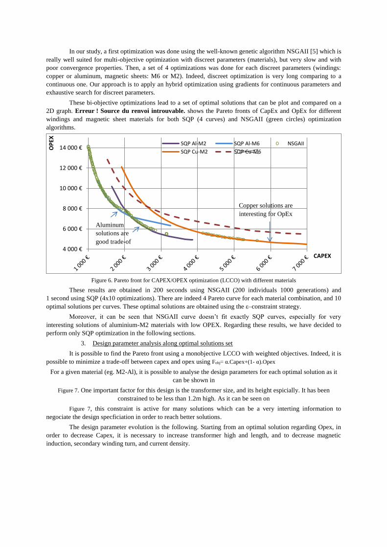
These bi-objective optimizations lead to a set of optimal solutions that can be plot and compared on a
2D graph. Erreur ! Source du renvoi introuvable. shows the Pareto fronts of CapEx and OpEx for different
windings and magnetic sheet materials for both SQP (4 curves) and NSGAII (green circles) optimization
algorithms.
Figure 6. Pareto front for CAPEX/OPEX optimization (LCCO) with different materials
These results are obtained in 200 seconds using NSGAII (200 individuals 1000 generations) and
1 second using SQP (4x10 optimizations). There are indeed 4 Pareto curve for each material combination, and 10
optimal solutions per curves. These optimal solutions are obtained using the ε–constraint strategy.
Moreover, it can be seen that NSGAII curve doesn’t fit exactly SQP curves, especially for very
interesting solutions of aluminium-M2 materials with low OPEX. Regarding these results, we have decided to
perform only SQP optimization in the following sections.
3. Design parameter analysis along optimal solutions set
It is possible to find the Pareto front using a monobjective LCCO with weighted objectives. Indeed, it is
possible to minimize a trade-off between capex and opex using Fobj= α.Capex+(1- α).Opex
For a given material (eg. M2-Al), it is possible to analyse the design parameters for each optimal solution as it
can be shown in
Figure 7. One important factor for this design is the transformer size, and its height espicially. It has been
constrained to be less than 1.2m high. As it can be seen on
Figure 7, this constraint is active for many solutions which can be a very interting information to
negociate the design specficiation in order to reach better solutions.
The design parameter evolution is the following. Starting from an optimal solution regarding Opex, in
order to decrease Capex, it is necessary to increase transformer high and length, and to decrease magnetic
induction, secondary winding turn, and current density.
4 000 €
6 000 €
8 000 €
10 000 €
12 000 €
14 000 €OP
EX
CAPEX
SQP Al-M2 SQP Al-M6 NSGAII
SQP Cu-M2 SQP Cu-M6
Copper solutions are
interesting for OpEx
Aluminum
solutions are
good trade-of

Figure 7. (left) Al-M2 design parameters for optimal solutions regarding CAPEX/OPEX trade-off
(right) Al-M2 pptimal geometry for very low Opex value (α = 0.1)
4. Life Cycle Cost Optimization (LCCO) conclusions
In conclusions, two optimization algorithms have been used and compared. First, a derivative free
alogorithm has been used because it is easy to connect with a lot of model implementations and it is well suited
for discreet parameters. But, on the other side, it has bad convergence properties, especially when the number of
constraint increase. So a gradient based algorithm has been used with the help of an automatic generation of the
model’s Jacobian. Discreet parameters have been treated using exhaustive search beacause there where few of
them. Multi-objective has been managed using two different technics, the epsilon-constraint technic, and the
weighted objective technic. Both have given very accurate pareto front, very fast.
These multi-objective technics have been applied to study the Life Cycle Cost Optimization (LCCO)
Capex/Opex trade-off of the transformer, based on Pareto front solutions and design parameter variations. These
tools are very useful for designer to help him making choices between financial objectives. But what about these
methodology including environmental objectives ?
ENVIRONMENTAL IMPACTS
1. Life Cycle Analysis (LCA)
Most of time, the LCA is done in a sequential process, after the technico-economic design that we just
have made. The transformer is analyzed over its lifetime (Raw material acquisition; Manufacturing;
Transportation; Use; Recycling and end of life treatments), and a list of environmental impacts is computed as
described in Table 1:
Figure 8. Life Cycle Analysis
LCA is strongly related to the data base which is used. Here we are using EcoInvent Database
(www.ecoinvent.org/database) from the Swiss Centre for Life Cycle Inventories.
Non-Renewable resources: NR energy consumption (MJ)
Resources depletion (kg Sb)
Global warming potential: Greenhouse effect (kg CO2)
Air pollution: Acidification (kg SO2)
Photochemical oxidation (kg PO43)
Water pollution: Eutrophication potential (kg C2H4)
Toxicity: Aquatic eco-toxicity (1,4-DB)
Human toxicity (1,4-DB)
to low Opex to low Capex
LCA

It is possible to synthetize the LCA in two parts. The first is related to the transformer production phase,
in which we are including material and process as well as end of life of some reused materials. So, it is strongly
related to the masse (or volume) of the windings and the magnetic core, and their materials (Copper/Aluminium,
M2/M6). The second part is related to the transformer use phase, in which we are including energy consumption,
defined by Iron and Joule losses. The impacts are strongly related to the mix of energy production of the
localization. In this study we are using a European average.
It is amazing to see that LCA is depending on criteria that are very similar to the life cycle cost study we
have made previously. Indeed, it is possible to associate Production phase to CAPEX and Use phase to OPEX.
In the following figure, we are analyzing three solutions that are in the CAPEX/OPEX Pareto front.
They are corresponding to different weights α (Fobj= α.Capex+(1- α).Opex) in Figure 9 (left). Al-M6 (α=0.25) is good
for CAPEX, Cu-M6 (α=0.75) is good for OPEX, and Al-M2 (α=0.5) is a good trade-off.
In Figure 9 (right), we are comparing the environmental impacts for the three solutions. It is noticeable
that no solution is better than another. So there are also compromises to do for environmental impacts.
Nevertheless it can be see that the good CAPEX solution (Al-M6) is very poor for many impacts. Moreover, the
good trade-off solution (Al-M2) for life cycle cost, is also a good trade-off for Life Cycle Analysis.
Figure 9. (left) Three LCCO solutions in the CAPEX/OPEX Pareto front
(right) Comparison of the environmental impacts for the three LCCO solutions.
2. Life Cycle Impacts Optimization (LCIO)
In this work, we have developed a model computing environmental impacts, which can be used for Life Cycle
Impacts Optimization (LCIO). This model is using input parameters, such as mass of materials, production
process information and recycle percentage for each material, or energy consumption. It computes 8 impacts for
production and use phases, using coefficients that are defined in EcoInvent database (see 4 examples on
Table 1). It has been introduced in our modeling framework CADES and is then available to make a Life Cycle
Impacts Optimization (LCIO). A single objective function have defined based on a sum of each 8 impacts
normalized using the European Average per Day (EAD) normalization coefficients (last column of Table 1).
Table 1. 4 Exemples of coefficients from EcoInvent 2.0.
(last column) : EAD is used as normalization factor to create a single objective
aluminium, production
mix, at plant
(Product) (per kg)
aluminium product manufacturing,
average metal working
(Process) (per kg)
transport, freight, rail
RER (per t.km)
electricity, medium voltage,
production RER, at grid
(per kWh)
European
Average per Day
(EAD)
NR energy consumption (MJ) 112,7274401 49,57111391 0,71171048 10,08940245 420
Resources depletion (kg Sb) 0,049345 0,020776 0,00027766 0,0036969 0,0956
Greenhouse effect (kg CO2) 8,3368 3,2937 0,03948 0,50033 28,1
Acidification (kg SO2) 0,039461 0,013921 0,00021277 0,0022302 0,1226
Photochemical oxidation (kg
PO43)
0,014178 0,0062934 0,00010458 0,0014513 0,105
Eutrophication potential (kg C2H4) 0,0032852 0,00096405 8,9195E-06 0,000088696 0,015
Aquatic eco-toxicity (1,4-DB) 5,7428 2,0306 0,016637 0,23678 2,8
Human toxicity (1,4-DB) 40,603 9,8988 0,026284 0,24565 56,3

Figure 10 (left) is showing the 8 impacts for the 3 optimal previous solutions from the CAPEX/OPEX
Economic optimization (same than Figure 9 (right)).
Figure 10 (right) is showing the 8 impacts for the 3 new optimal solutions obtained using only
environmental impacts minimization for 3 material configurations (Al-M6, Al-M2 and Cu-M6). Both graphics
are using the same scale in order to be compared together.
Figure 10. (left) LCA of the three previous solutions from the Life Cycle Cost Optimization (LCCO)
(right) LCA of the new three solutions from the Life Cycle Impacts Optimization (LCIO).
A first result is that all 8 objectives are well balanced even if we have used a mono-objective
optimization using a weighted sum. A second result is that we have decreased significantly the impacts for a
given material configuration. A consequence is the increase of the cost. The comparison between Total costs
(CAPEX+OPEX) and Total Impacts (sum of the 8 normalized environmental impacts) can be made, based on
the Figure 11. On the one hand, it can be noticed that, for each material configurations (Al-M6, Al-M2 and Cu-
M2), the total costs, when optimizing costs (LCCO), is better than total cost when optimizing environmental
impacts. The same conclusion can be made for impacts when they are optimized. On the other hand, the increase
of impacts (resp. of costs) when optimizing cost (resp. impacts) is very small.
Figure 11. Comparison of total costs and total impact for LCCO and LCIO
In order to study more about this trade-off (total costs and total impacts) we have performed a multi-
objective optimization. The Pareto front can be seen on Figure 12. This Pareto is very small regarding to the full
scale. Indeed, the variation is only of 4% for both Life Cycle Impacts and Life Cycle Costs. The conclusion is
that optimizing LCC of LCI is very similar in results.
0
5000
10000
15000Total Costs Total Impacts
LCCO LCIO LCCO LCIO LCCO LCIOAl-M6 Al-M2 Cu-M2
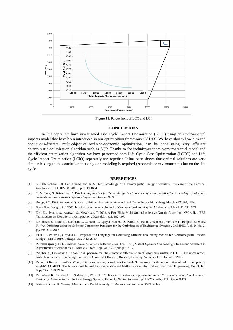
Figure 12. Pareto front of LCC and LCI
CONCLUSIONS
In this paper, we have investigated Life Cycle Impact Optimization (LCIO) using an environmental
impacts model that have been introduced in our optimization framework CADES. We have shown how a mixed
continuous-discrete, multi-objective technico-economic optimization, can be done using very efficient
deterministic optimization algorithm such as SQP. Thanks to the technico-economic-environmental model and
the efficient optimization algorithm, we have performed both Life Cycle Cost Optimization (LCCO) and Life
Cycle Impact Optimization (LCIO) separately and together. It has been shown that optimal solutions are very
similar leading to the conclusion that only one modeling is required (economic or environmental) but on the life
cycle.
REFERENCES
[1] V. Debusschere, , H. Ben Ahmed, and B. Multon, Eco-design of Electromagnetic Energy Converters: The case of the electrical
transformer, IEEE IEMDC 2007, pp. 1599-1604
[2] T. V. Tran, S. Brisset and P. Brochet, Approaches for the ecodesign in electrical engineering application to a safety transformer,
International conference on Systems, Signals & Devices 2009
[3] Boggs, P.T. 1996. Sequential Quadratic, National Institute of Standards and Technology, Gaithersburg, Maryland 20899, USA.
[4] Potra, F.A., Wright, S.J. 2000. Interior-point methods, Journal of Computational and Applied Mathematics 124 (1–2): 281–302.
[5] Deb, K., Pratap, A., Agarwal, S., Meyarivan, T. 2002. A Fast Elitist Multi-Optimal objective Genetic Algorithm: NSGA-II, . IEEE
Transactions on Evolutionary Computation , 6(2)vol.6, no. 2: 182-197.
[6] Delinchant B., Duret D., Estrabaut L., Gerbaud L., Nguyen Huu H., Du Peloux B., Rakotoarison H.L., Verdiere F., Bergeon S.; Wurtz
F., “An Optimizer using the Software Component Paradigm for the Optimization of Engineering Systems”, COMPEL, Vol. 26 No. 2,
pp. 368-379, 2007
[7] Enciu P., Wurtz F., Gerbaud L., “Proposal of a Language for Describing Differentiable Sizing Models for Electromagnetic Devices
Design”, CEFC 2010, Chicago, May 9-12, 2010
[8] P. Pham-Quang, B. Delinchant. “Java Automatic Differentiation Tool Using Virtual Operator Overloading”. In Recent Advances in
Algorithmic Differentiation. S. Forth et al. (eds.), pp 241-250, Springer; 2012.
[9] Walther A., Griewank A., Adol-C : A package for the automatic differentiation of algorithms written in C/C++, Technical report,
Institute of Scientic Computing, Technische Universitat Dresden, Dresden, Germany, Version 2.0.0, December 2008
[10] Benoit Delinchant, Frédéric Wurtz, João Vasconcelos, Jean-Louis Coulomb "Framework for the optimization of online computable
models", COMPEL: The International Journal for Computation and Mathematics in Electrical and Electronic Engineering, Vol. 33 Iss:
3, pp.745 – 758, 2014
[11] Delinchant B., Estrabaud L., Gerbaud L., Wurtz F. “Multi-criteria design and optimization tools (53 pages)” chapter 5 of Integrated
Design by Optimization of Electrical Energy Systems, Edited by Xavier Roboam, pp 193-245, Wiley ISTE (june 2012).
[12] Ishizaka, A. and P. Nemery, Multi-criteria Decision Analysis: Methods and Software. 2013: Wiley.