
Lecture Notes-Multiple Antennas for MIMO Communications - Basic Theory
48
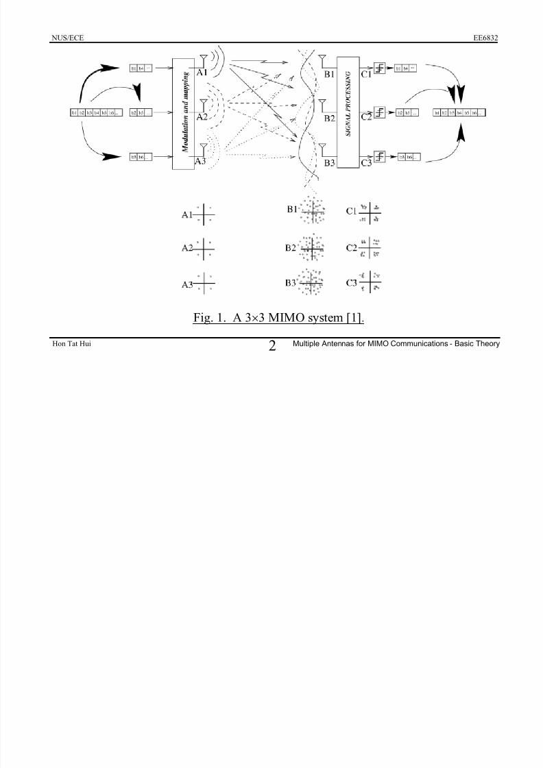
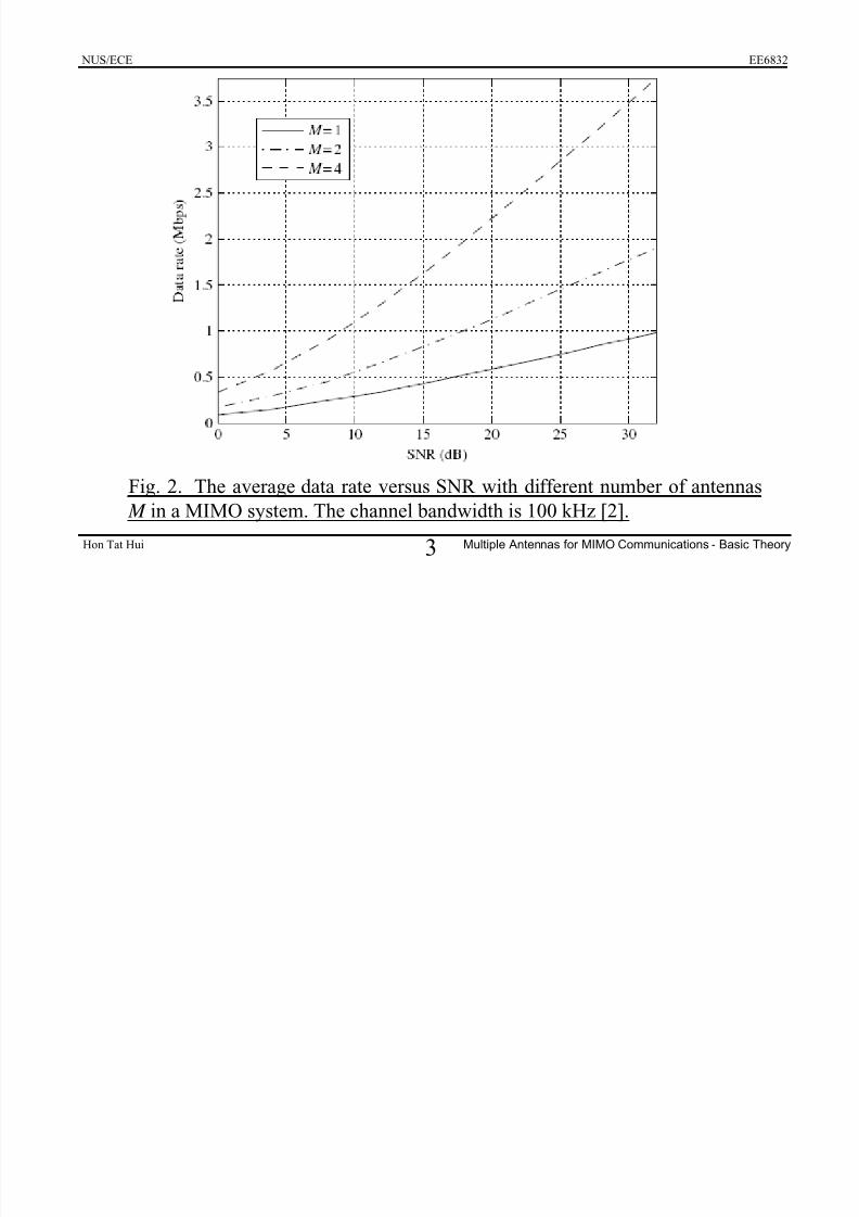
Hon Tat Hui Multiple Antennas for MIMO Communications - Basic Theory NUS/ECE EE6832 1 Multiple Antennas for MIMO Communications - Basic Theory 1 Introduction The multiple-input multiple-output (MIMO) technology (Fig. 1) is a breakthrough in wireless communication system design. It uses the spatial dimension (provided by the multiple antennas at the transmitter and the receiver) to combat the multipath fading effect. Fig. 2 shows the dramatic increase in transmission data rate with the increase in the number of transmitting and receiving antennas M of a MIMO system.
-
Upload
gowthamkurri -
Category
Documents
-
view
233 -
download
1
Transcript of Lecture Notes-Multiple Antennas for MIMO Communications - Basic Theory

8/13/2019 Lecture Notes-Multiple Antennas for MIMO Communications - Basic Theory
http://slidepdf.com/reader/full/lecture-notes-multiple-antennas-for-mimo-communications-basic-theory 1/48
Hon Tat Hui Multiple Antennas for MIMO Communications - Basic Theory
NUS/ECE EE6832
1
Multiple Antennas forMIMO Communications - Basic Theory
1 Introduction
The multiple-input multiple-output (MIMO) technology
(Fig. 1) is a breakthrough in wireless communicationsystem design. It uses the spatial dimension (provided by
the multiple antennas at the transmitter and the receiver) to
combat the multipath fading effect. Fig. 2 shows the
dramatic increase in transmission data rate with the
increase in the number of transmitting and receiving
antennas M of a MIMO system.
8/13/2019 Lecture Notes-Multiple Antennas for MIMO Communications - Basic Theory
http://slidepdf.com/reader/full/lecture-notes-multiple-antennas-for-mimo-communications-basic-theory 2/48
Hon Tat Hui Multiple Antennas for MIMO Communications - Basic Theory
NUS/ECE EE6832
2
Fig. 1. A 33 MIMO system [1].
8/13/2019 Lecture Notes-Multiple Antennas for MIMO Communications - Basic Theory
http://slidepdf.com/reader/full/lecture-notes-multiple-antennas-for-mimo-communications-basic-theory 3/48
Hon Tat Hui Multiple Antennas for MIMO Communications - Basic Theory
NUS/ECE EE6832
3
Fig. 2. The average data rate versus SNR with different number of antennas
M in a MIMO system. The channel bandwidth is 100 kHz [2].
8/13/2019 Lecture Notes-Multiple Antennas for MIMO Communications - Basic Theory
http://slidepdf.com/reader/full/lecture-notes-multiple-antennas-for-mimo-communications-basic-theory 4/48
Hon Tat Hui Multiple Antennas for MIMO Communications - Basic Theory
NUS/ECE EE6832
4
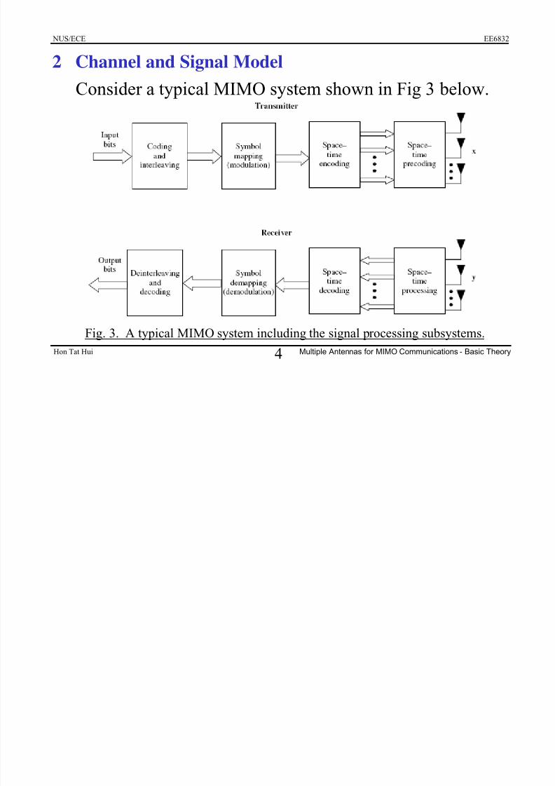
2 Channel and Signal ModelConsider a typical MIMO system shown in Fig 3 below.
Fig. 3. A typical MIMO system including the signal processing subsystems.
8/13/2019 Lecture Notes-Multiple Antennas for MIMO Communications - Basic Theory
http://slidepdf.com/reader/full/lecture-notes-multiple-antennas-for-mimo-communications-basic-theory 5/48
Hon Tat Hui Multiple Antennas for MIMO Communications - Basic Theory
NUS/ECE EE6832
5
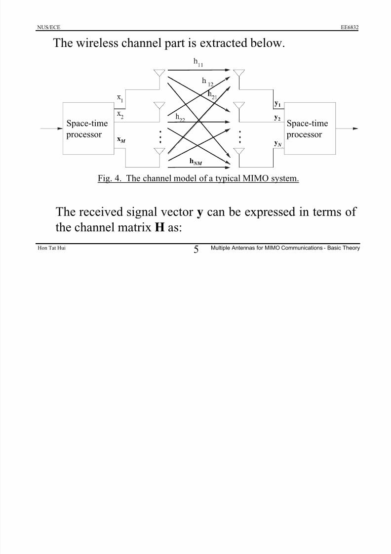
The wireless channel part is extracted below.
The received signal vector y can be expressed in terms of
the channel matrix H as:
Fig. 4. The channel model of a typical MIMO system.
Space-time
processor
Space-time
processor
y N
y2
y1
x M
h NM

8/13/2019 Lecture Notes-Multiple Antennas for MIMO Communications - Basic Theory
http://slidepdf.com/reader/full/lecture-notes-multiple-antennas-for-mimo-communications-basic-theory 6/48
Hon Tat Hui Multiple Antennas for MIMO Communications - Basic Theory
NUS/ECE EE6832
6
y Hx n
1
2
1
2
received signal vector
transmitted signal vector
N
M
y y
y
x
x
x
y
x
where the symbols are:(1)
(2)
(3)

8/13/2019 Lecture Notes-Multiple Antennas for MIMO Communications - Basic Theory
http://slidepdf.com/reader/full/lecture-notes-multiple-antennas-for-mimo-communications-basic-theory 7/48
Hon Tat Hui Multiple Antennas for MIMO Communications - Basic Theory
NUS/ECE EE6832
7
11 12 1
21 22 2
1 2
1
2
channel matrix
noise vector
M
M
N N NM
M
h h hh h h
h h h
n
n
n
H
n
Thereafter, we study the transmit power PT constrained
MIMO systems only, i.e., PT C for some fixed C . We
can also write:
(5)
(4)
8/13/2019 Lecture Notes-Multiple Antennas for MIMO Communications - Basic Theory
http://slidepdf.com/reader/full/lecture-notes-multiple-antennas-for-mimo-communications-basic-theory 8/48
Hon Tat Hui Multiple Antennas for MIMO Communications - Basic Theory
NUS/ECE EE6832
8
2 2 21 2
H T M P x x x C x x (6)
The covariance matrices of the transmitted signals andreceived signals are:
H
xx
H
yy
H H H
E
E
E E
R xx
R yy
Hxx H nn
2.1 The Covariance Matrices
The covariance matrices are important parameters to
characterize a MIMO communication system.
(7)
8/13/2019 Lecture Notes-Multiple Antennas for MIMO Communications - Basic Theory
http://slidepdf.com/reader/full/lecture-notes-multiple-antennas-for-mimo-communications-basic-theory 9/48
Hon Tat Hui Multiple Antennas for MIMO Communications - Basic Theory
NUS/ECE EE6832
9
The traces ofR
xx andR
yy give the total powers of thetransmitted and received signals, respectively. The off-
diagonal elements of R xx and R yy give the correlations
between the signals at different antenna elements.
Consider a symbol period of time T s, for the transmitted
signals, it is usually made such that:
H
xx M E R xx I
H H H
yy
H H
nn
H
nn
E E
E
R Hxx H nn
H xx H R
HH R
Then within T s,(8)
(9)
8/13/2019 Lecture Notes-Multiple Antennas for MIMO Communications - Basic Theory
http://slidepdf.com/reader/full/lecture-notes-multiple-antennas-for-mimo-communications-basic-theory 10/48
Hon Tat Hui Multiple Antennas for MIMO Communications - Basic Theory
NUS/ECE EE6832
10
where Rnn
is the noise covariance matrix. In (8) and (9),
we have assumed that the channels are stable within T s.
Thus over a longer period of time (>> T s), the average
received signal covariance matrix is:
H
yy nn E R HH R (10)
From (10), it can be seen that the received signal power is
determined by the channel covariance matrix E {HH H }
and the noise covariance matrix Rnn. As Rnn is
determined by the environment and cannot be changed,
we can manipulate or select an H to optimize the channel
output SNR (so as the capacity) of the MIMO system.
8/13/2019 Lecture Notes-Multiple Antennas for MIMO Communications - Basic Theory
http://slidepdf.com/reader/full/lecture-notes-multiple-antennas-for-mimo-communications-basic-theory 11/48
Hon Tat Hui Multiple Antennas for MIMO Communications - Basic Theory
NUS/ECE EE6832
11
3 Channel Capacity
The channel capacity C of a single-input single-output
(SISO) system is given by [3]:
2log 1 bit/sC B S N
where B (in Hz) is the channel bandwidth, S (in Watt) isthe signal power, and N (in Watt) is the noise power.
Both S and N are measured at the output of the channel.
The channel capacity is a measure of the maximum rate
that information (in bits) can be transmitted through the
channel with an arbitrarily small error after using a
certain coding method.
(11)
3.1 For SISO Systems
8/13/2019 Lecture Notes-Multiple Antennas for MIMO Communications - Basic Theory
http://slidepdf.com/reader/full/lecture-notes-multiple-antennas-for-mimo-communications-basic-theory 12/48
Hon Tat Hui Multiple Antennas for MIMO Communications - Basic Theory
NUS/ECE EE6832
12
Example 1
A black-and-white TV screen picture may be considered as
composed of approximately 3105 picture elements. Assume
that each picture element has 10 brightness levels each beingequally likely to occur. TV signals are transmitted at 30
picture frames per second. The signal-to-noise ratio at the
TV is required to be at least 30 dB. What is the required
channel bandwidth for TV broadcast?
Solutions
Information per picture element = log210 = 3.32 bits
Information per picture frame = 3.323105 = 9.96105 bits
8/13/2019 Lecture Notes-Multiple Antennas for MIMO Communications - Basic Theory
http://slidepdf.com/reader/full/lecture-notes-multiple-antennas-for-mimo-communications-basic-theory 13/48
Hon Tat Hui Multiple Antennas for MIMO Communications - Basic Theory
NUS/ECE EE6832
13
As 30 picture frames are transmitting per second, therefore
the maximum information rate, R, for the TV transmission is
then:5
6
30 9.96 10
29.9 10 bit/s
R
This maximum information rate is the channel capacity C
for TV broadcast. That is, 6
229.9 10 log 1 R C B S N
Therefore the bandwidth B can be calculated as:
66
2 2
29.9 103 10 3 MHz
log 1 log 1 1000
C B
S N
8/13/2019 Lecture Notes-Multiple Antennas for MIMO Communications - Basic Theory
http://slidepdf.com/reader/full/lecture-notes-multiple-antennas-for-mimo-communications-basic-theory 14/48
Hon Tat Hui Multiple Antennas for MIMO Communications - Basic Theory
NUS/ECE EE6832
14
For a MIMO system, the calculation of the capacity is
more complicated due to the determination of the signal-
to-noise ratio S / N .
Consider a MIMO system with a channel matrix H
( N M ) as below:
3.2 For MIMO Systems
y Hx n
By the singular value decomposition (SVD) theorem [4],
any N M matrix H can be written as:
H H UDV
where D is an N M a diagonal matrix with non-negative
elements, U is an N N unitary matrix, and V is a M M
(12)
(13)
8/13/2019 Lecture Notes-Multiple Antennas for MIMO Communications - Basic Theory
http://slidepdf.com/reader/full/lecture-notes-multiple-antennas-for-mimo-communications-basic-theory 15/48
8/13/2019 Lecture Notes-Multiple Antennas for MIMO Communications - Basic Theory
http://slidepdf.com/reader/full/lecture-notes-multiple-antennas-for-mimo-communications-basic-theory 16/48
Hon Tat Hui Multiple Antennas for MIMO Communications - Basic Theory
NUS/ECE EE6832
16
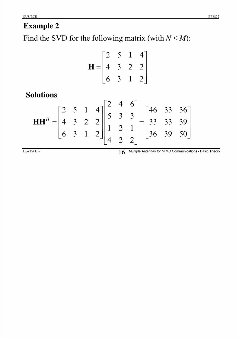
Example 2
Find the SVD for the following matrix (with N < M ):
2 5 1 4
4 3 2 2
6 3 1 2
H
Solutions
2 4 62 5 1 4 46 33 36
5 3 34 3 2 2 33 33 391 2 1
6 3 1 2 36 39 504 2 2
H
HH

8/13/2019 Lecture Notes-Multiple Antennas for MIMO Communications - Basic Theory
http://slidepdf.com/reader/full/lecture-notes-multiple-antennas-for-mimo-communications-basic-theory 17/48
Hon Tat Hui Multiple Antennas for MIMO Communications - Basic Theory
NUS/ECE EE6832
17
The eigenvalues of HH H are:
1 = 115.5900, 2 = 12.4511, 3 = 0.9588
Therefore,
115.5900 0 0 0
0 12.4511 0 0
0 0 0.9588 0
D
By using Matlab with the command: [U,S,V]=svd(H), we
can find the SVD of H as:

8/13/2019 Lecture Notes-Multiple Antennas for MIMO Communications - Basic Theory
http://slidepdf.com/reader/full/lecture-notes-multiple-antennas-for-mimo-communications-basic-theory 18/48
Hon Tat Hui Multiple Antennas for MIMO Communications - Basic Theory
NUS/ECE EE6832
18
0.5741 0.7951 0.1955
0.5258 -0.1749 -0.8324
0.6277 -0.5806 0.5185
10.7513 0 0 0
0 3.5286 0 0
0 0 0.9792 00.6527 -0.7349 0.1759 -0.0538
0.5888 0.4843 0.0363 0.6461 0.
H
H UDV
2096 -0.0384 -0.9711 -0.1077
0.4282 0.4731 0.1573 -0.7537
H
8/13/2019 Lecture Notes-Multiple Antennas for MIMO Communications - Basic Theory
http://slidepdf.com/reader/full/lecture-notes-multiple-antennas-for-mimo-communications-basic-theory 19/48
Hon Tat Hui Multiple Antennas for MIMO Communications - Basic Theory
NUS/ECE EE6832
19
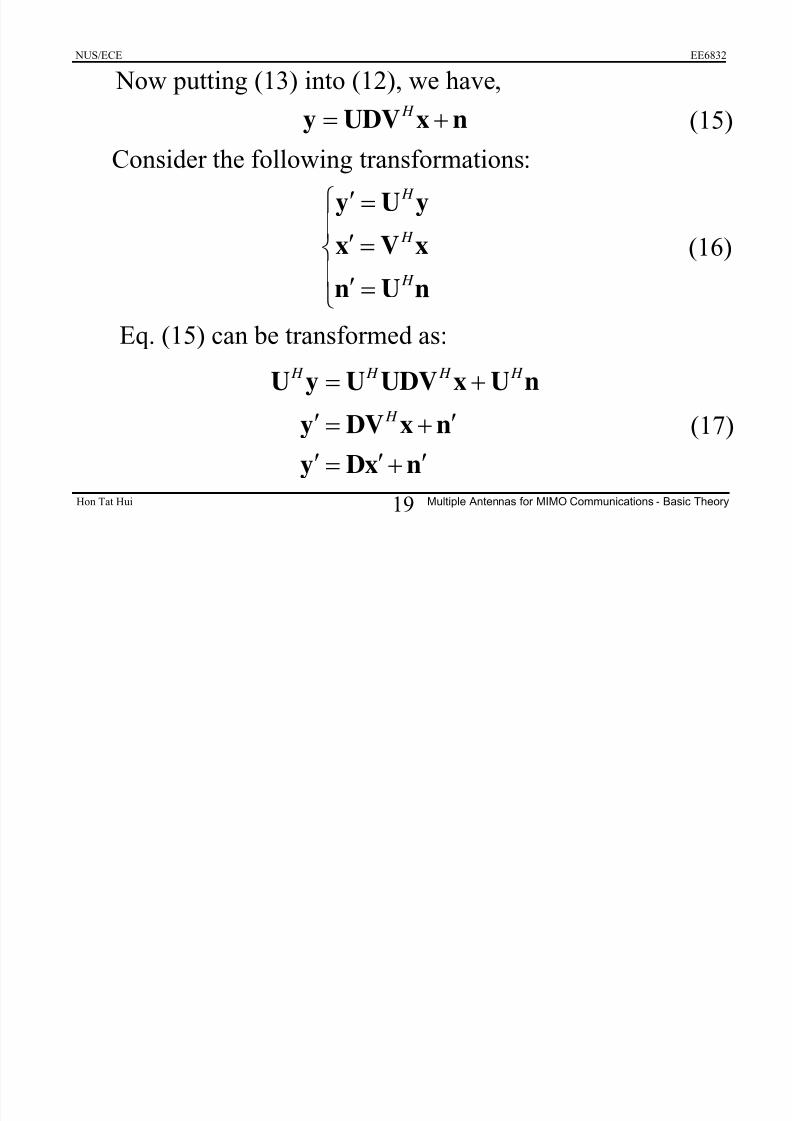
H y UDV x n
Consider the following transformations:
H
H
H
y U y
x V x
n U n
(15)
H H H H
H
U y U UDV x U ny DV x n
y Dx n
Eq. (15) can be transformed as:
(16)
(17)
Now putting (13) into (12), we have,
8/13/2019 Lecture Notes-Multiple Antennas for MIMO Communications - Basic Theory
http://slidepdf.com/reader/full/lecture-notes-multiple-antennas-for-mimo-communications-basic-theory 20/48
Hon Tat Hui Multiple Antennas for MIMO Communications - Basic Theory
NUS/ECE EE6832
20
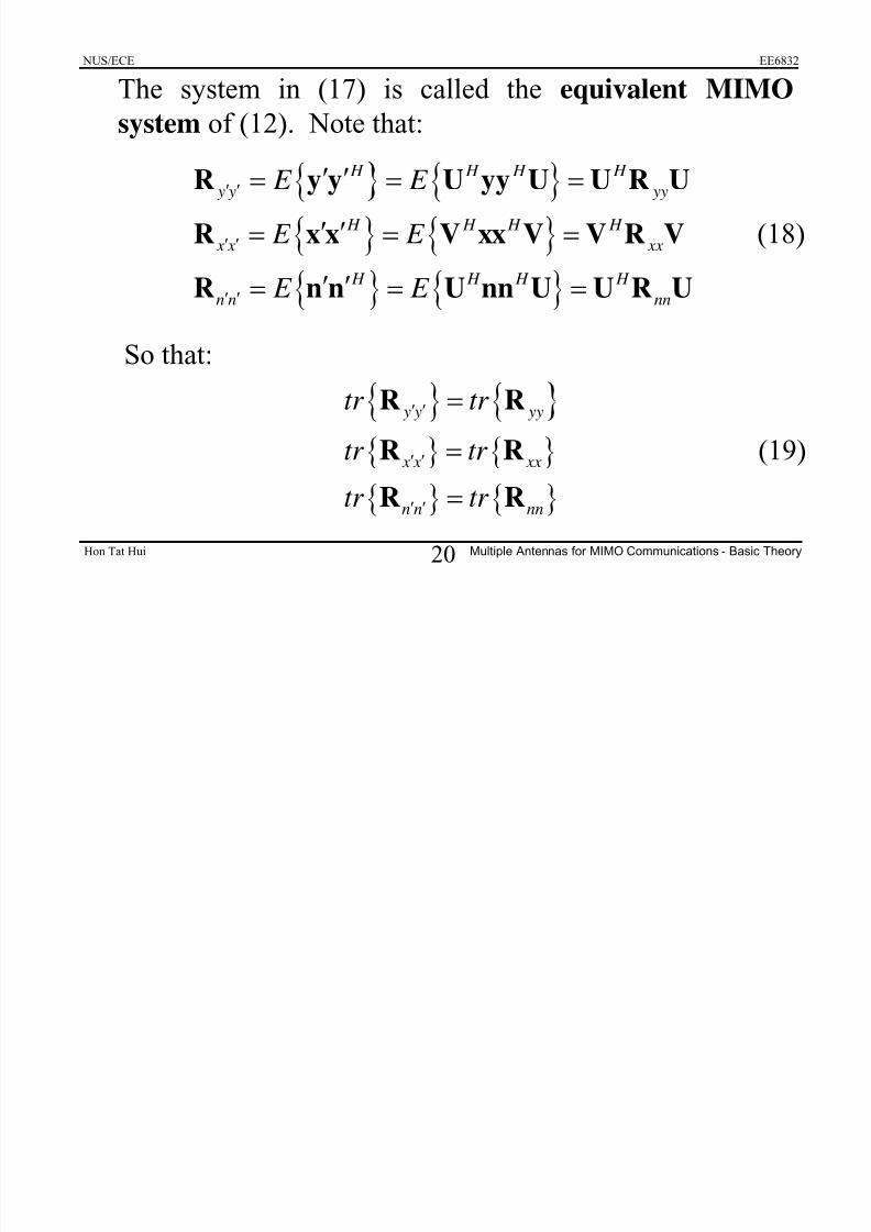
The system in (17) is called the equivalent MIMO
system of (12). Note that:
H H H H
y y yy
H H H H
x x xx
H H H H
n n nn
E E
E E
E E
R y y U yy U U R U
R x x V xx V V R V
R n n U nn U U R U
So that:
y y yy
x x xx
n n nn
tr tr
tr tr
tr tr
R R
R R
R R
(18)
(19)
8/13/2019 Lecture Notes-Multiple Antennas for MIMO Communications - Basic Theory
http://slidepdf.com/reader/full/lecture-notes-multiple-antennas-for-mimo-communications-basic-theory 21/48
Hon Tat Hui Multiple Antennas for MIMO Communications - Basic Theory
NUS/ECE EE6832
21
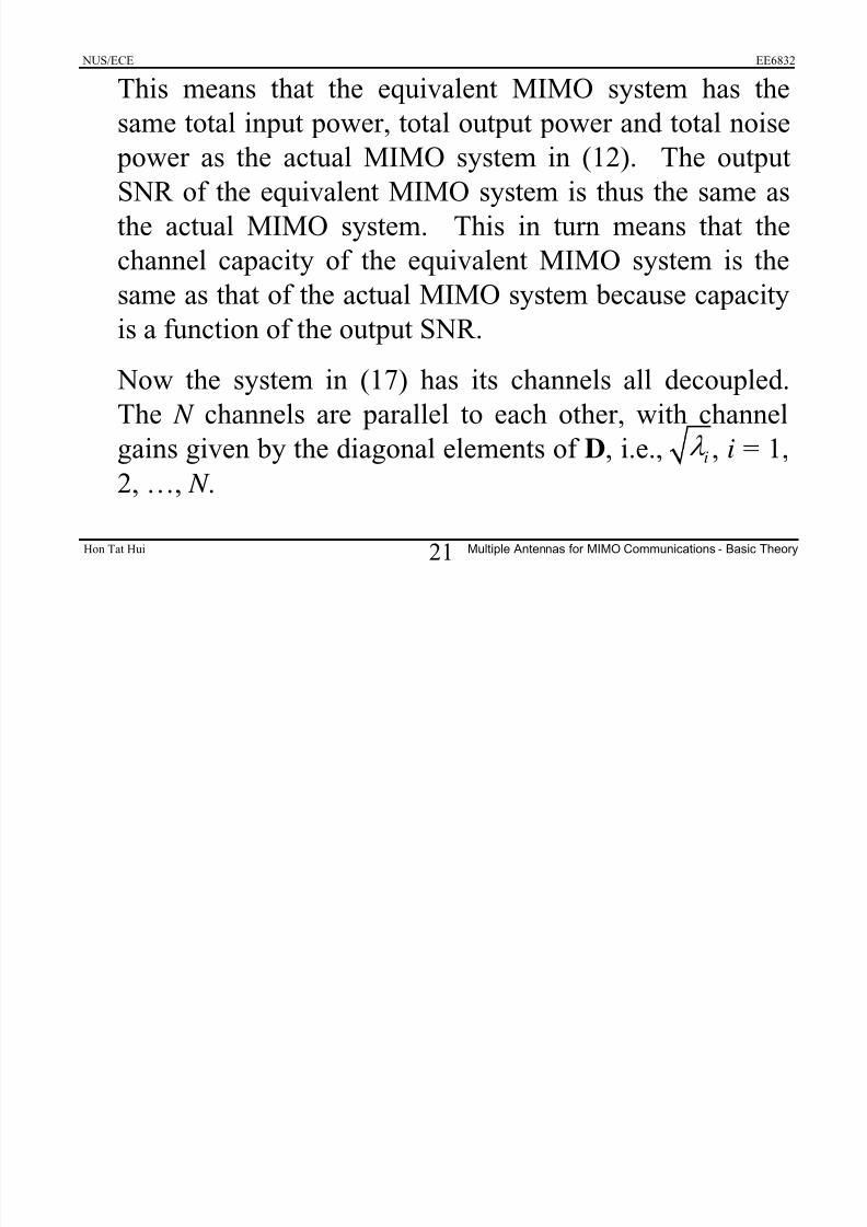
This means that the equivalent MIMO system has the
same total input power, total output power and total noise
power as the actual MIMO system in (12). The output
SNR of the equivalent MIMO system is thus the same as
the actual MIMO system. This in turn means that thechannel capacity of the equivalent MIMO system is the
same as that of the actual MIMO system because capacity
is a function of the output SNR.
Now the system in (17) has its channels all decoupled.
The N channels are parallel to each other, with channel
gains given by the diagonal elements of D, i.e., , i = 1,
2, , N .i
8/13/2019 Lecture Notes-Multiple Antennas for MIMO Communications - Basic Theory
http://slidepdf.com/reader/full/lecture-notes-multiple-antennas-for-mimo-communications-basic-theory 22/48
Hon Tat Hui Multiple Antennas for MIMO Communications - Basic Theory
NUS/ECE EE6832
22
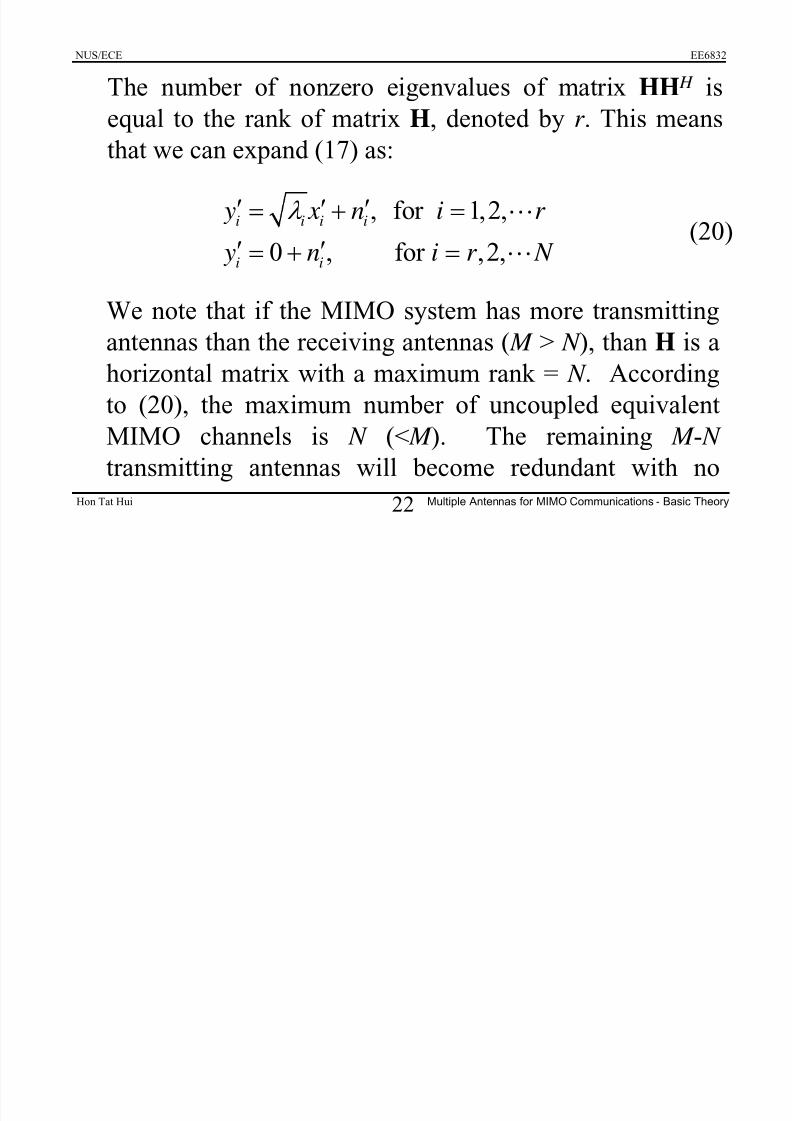
The number of nonzero eigenvalues of matrix HH H is
equal to the rank of matrix H, denoted by r . This means
that we can expand (17) as:
, for 1,2,
0 , for ,2,
i i i i
i i
y x n i r
y n i r N
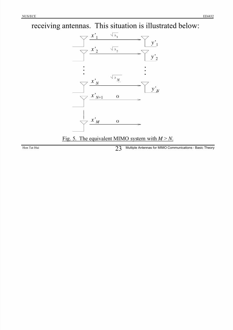
We note that if the MIMO system has more transmitting
antennas than the receiving antennas ( M > N ), than H is a
horizontal matrix with a maximum rank = N . According
to (20), the maximum number of uncoupled equivalent
MIMO channels is N (< M ). The remaining M - N
transmitting antennas will become redundant with no
(20)
8/13/2019 Lecture Notes-Multiple Antennas for MIMO Communications - Basic Theory
http://slidepdf.com/reader/full/lecture-notes-multiple-antennas-for-mimo-communications-basic-theory 23/48
Hon Tat Hui Multiple Antennas for MIMO Communications - Basic Theory
NUS/ECE EE6832
23
receiving antennas. This situation is illustrated below: x’1
x’2
x’ N
x’ N +1
x’1
x’ M
y’1
y’2
y’ N
N
Fig. 5. The equivalent MIMO system with M > N .

8/13/2019 Lecture Notes-Multiple Antennas for MIMO Communications - Basic Theory
http://slidepdf.com/reader/full/lecture-notes-multiple-antennas-for-mimo-communications-basic-theory 24/48
Hon Tat Hui Multiple Antennas for MIMO Communications - Basic Theory
NUS/ECE EE6832
24
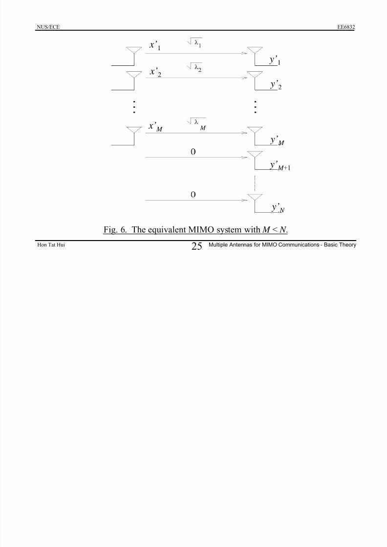
On the other hand, if the MIMO system has more
receiving antennas than the transmitting antennas ( M < N ),
than H is a vertical matrix with a maximum rank = M .
According to (20), the maximum number of uncoupled
equivalent MIMO channels is M (< N ). The remaining N - M receiving antennas will become redundant with no
received signals. This is illustrated on next page.
In general, for an N M MIMO system, the maximum
number of uncoupled equivalent channels is min( N , M ).
8/13/2019 Lecture Notes-Multiple Antennas for MIMO Communications - Basic Theory
http://slidepdf.com/reader/full/lecture-notes-multiple-antennas-for-mimo-communications-basic-theory 25/48
Hon Tat Hui Multiple Antennas for MIMO Communications - Basic Theory
NUS/ECE EE6832
25
Fig. 6. The equivalent MIMO system with M < N .
x’1
x’2
x’ M M
y’1
y’2
y’ M
y’ M +1
y’ N

8/13/2019 Lecture Notes-Multiple Antennas for MIMO Communications - Basic Theory
http://slidepdf.com/reader/full/lecture-notes-multiple-antennas-for-mimo-communications-basic-theory 26/48
Hon Tat Hui Multiple Antennas for MIMO Communications - Basic Theory
NUS/ECE EE6832
26
As the channels of the equivalent MIMO system in (17)
are uncoupled and parallel, the channel capacity of (17)can be calculated by a summation of the individual
capacities of the parallel channels. That is,
2 21
log 1 ir
y
i
PC B
(21)
where B (in Hz) is the channel bandwidth, (in Watt) isthe power received at the ith receiving antenna, 2 (in
Watt) is the noise power at the ith receiving antenna, and
r is the rank of H. In order to related the received power
to the channel parameters, we need to classify a MIMO
system according to the availability of the channel
knowledge to the transmitter or receiver.
i yP
8/13/2019 Lecture Notes-Multiple Antennas for MIMO Communications - Basic Theory
http://slidepdf.com/reader/full/lecture-notes-multiple-antennas-for-mimo-communications-basic-theory 27/48
Hon Tat Hui Multiple Antennas for MIMO Communications - Basic Theory
NUS/ECE EE6832
27
(A) Channel state information (CSI) known to the
receiver only
As the transmitter does not know the CSI, its best strategy
is to transmit power equally from all its transmittingantennas. For the equivalent MIMO system in (17), this
can be done by making all the elements of x’ to have the
same power. Under this situation, the received power is
then calculated as:
i y i
P
P
where P is the total transmitting power.
(22)
8/13/2019 Lecture Notes-Multiple Antennas for MIMO Communications - Basic Theory
http://slidepdf.com/reader/full/lecture-notes-multiple-antennas-for-mimo-communications-basic-theory 28/48
Hon Tat Hui Multiple Antennas for MIMO Communications - Basic Theory
NUS/ECE EE6832
28
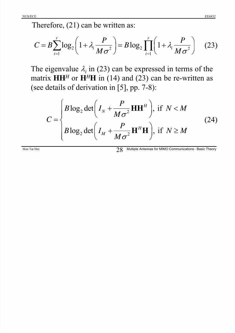
Therefore, (21) can be written as:
2 22 21 1
log 1 log 1r r
i i
i i
P PC B B
M M
The eigenvalue i in (23) can be expressed in terms of the
matrix HH H or H H H in (14) and (23) can be re-written as
(see details of derivation in [5], pp. 7-8):
(23)
2 2
2 2
log det , if
log det , if
H
N
H
M
P B I N M
M C P
B I N M M
HH
H H
(24)

8/13/2019 Lecture Notes-Multiple Antennas for MIMO Communications - Basic Theory
http://slidepdf.com/reader/full/lecture-notes-multiple-antennas-for-mimo-communications-basic-theory 29/48
Hon Tat Hui Multiple Antennas for MIMO Communications - Basic Theory
NUS/ECE EE6832
29
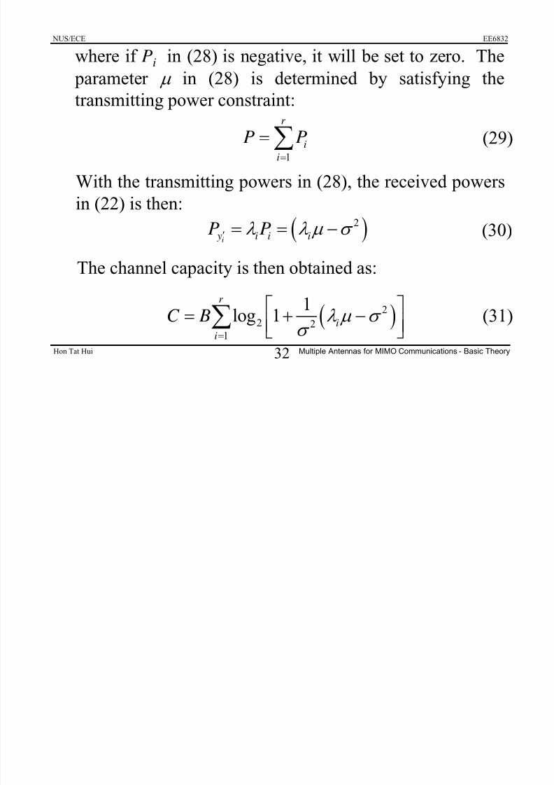
The total transmitting power P in (24) may not be easily
known. If the average received powers Pr at each of the
receiving antennas are the same, we have:
2 2
2 2
log det , if
log det , if
H
r N
loss
H
r M
loss
P B I N M
M P
C P B I N M
M P
HH
H H
r lossP P P where Ploss is the average path loss from the transmitter to
the receiver. Then (24) can be re-written as:
(25)
(26)

8/13/2019 Lecture Notes-Multiple Antennas for MIMO Communications - Basic Theory
http://slidepdf.com/reader/full/lecture-notes-multiple-antennas-for-mimo-communications-basic-theory 30/48
Hon Tat Hui Multiple Antennas for MIMO Communications - Basic Theory
NUS/ECE EE6832
30
2
2
log det , if
log det , if
H
N
loss
H
M loss
B I N M M PC
B I N M M P
HH
H H
Or, in terms of the SNR at the receiving antennas , we
have:
(27)
8/13/2019 Lecture Notes-Multiple Antennas for MIMO Communications - Basic Theory
http://slidepdf.com/reader/full/lecture-notes-multiple-antennas-for-mimo-communications-basic-theory 31/48
Hon Tat Hui Multiple Antennas for MIMO Communications - Basic Theory
NUS/ECE EE6832
31
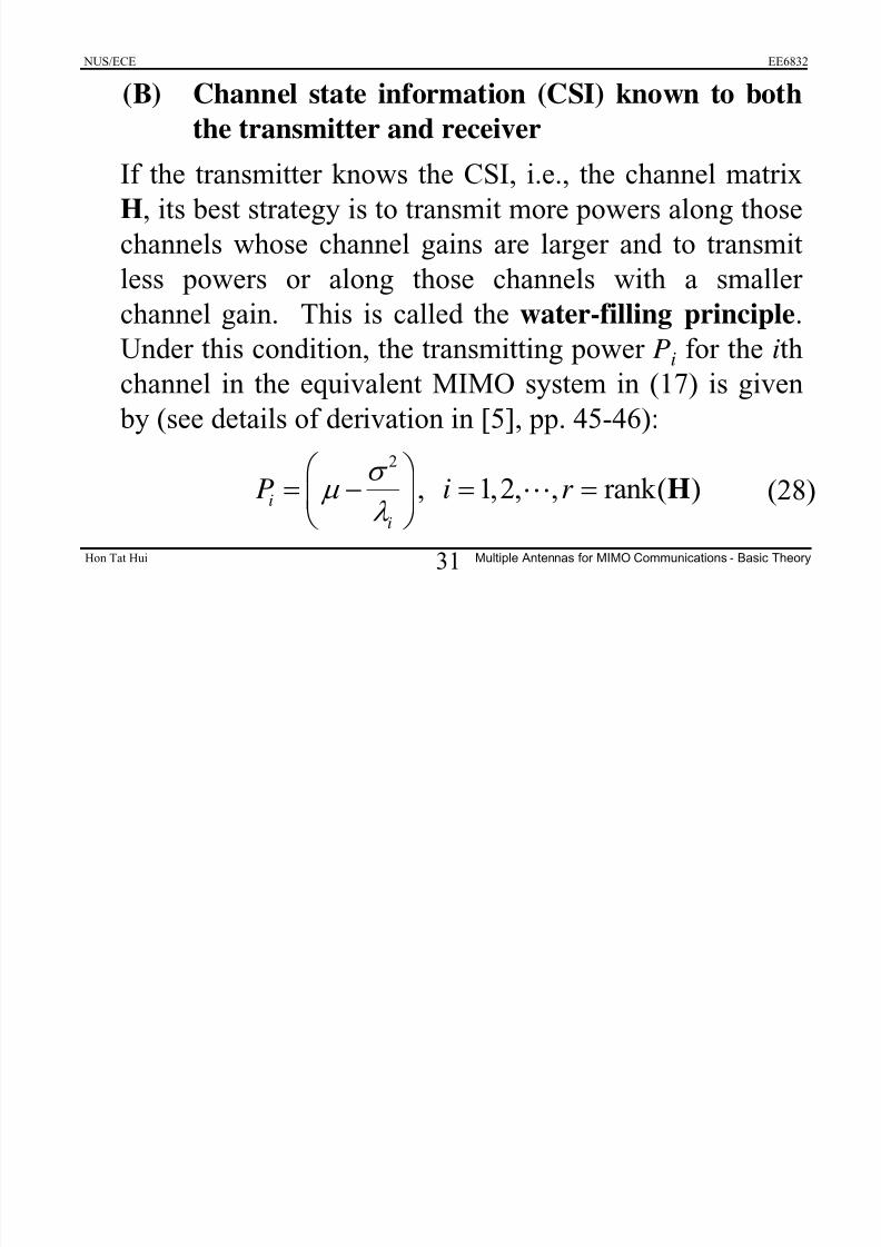
(B) Channel state information (CSI) known to both
the transmitter and receiver
If the transmitter knows the CSI, i.e., the channel matrix
H, its best strategy is to transmit more powers along those
channels whose channel gains are larger and to transmit
less powers or along those channels with a smaller
channel gain. This is called the water-filling principle.
Under this condition, the transmitting power Pi for the ith
channel in the equivalent MIMO system in (17) is given
by (see details of derivation in [5], pp. 45-46):
2
, 1,2, , rank( )i
i
P i r
H (28)
8/13/2019 Lecture Notes-Multiple Antennas for MIMO Communications - Basic Theory
http://slidepdf.com/reader/full/lecture-notes-multiple-antennas-for-mimo-communications-basic-theory 32/48
8/13/2019 Lecture Notes-Multiple Antennas for MIMO Communications - Basic Theory
http://slidepdf.com/reader/full/lecture-notes-multiple-antennas-for-mimo-communications-basic-theory 33/48
Hon Tat Hui Multiple Antennas for MIMO Communications - Basic Theory
NUS/ECE EE6832
33
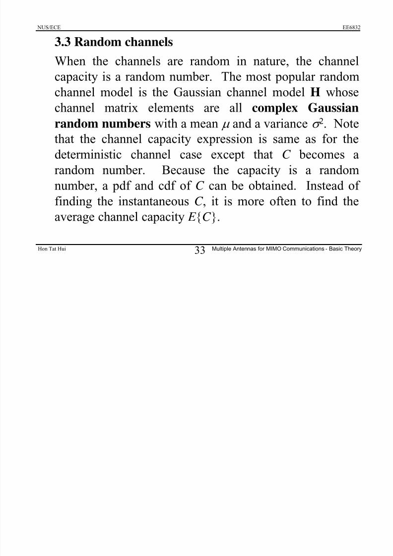
3.3 Random channels
When the channels are random in nature, the channel
capacity is a random number. The most popular random
channel model is the Gaussian channel model H whose
channel matrix elements are all complex Gaussian
random numbers with a mean and a variance 2. Note
that the channel capacity expression is same as for the
deterministic channel case except that C becomes a
random number. Because the capacity is a random
number, a pdf and cdf of C can be obtained. Instead of
finding the instantaneous C , it is more often to find theaverage channel capacity E {C }.
8/13/2019 Lecture Notes-Multiple Antennas for MIMO Communications - Basic Theory
http://slidepdf.com/reader/full/lecture-notes-multiple-antennas-for-mimo-communications-basic-theory 34/48
Hon Tat Hui Multiple Antennas for MIMO Communications - Basic Theory
NUS/ECE EE6832
34
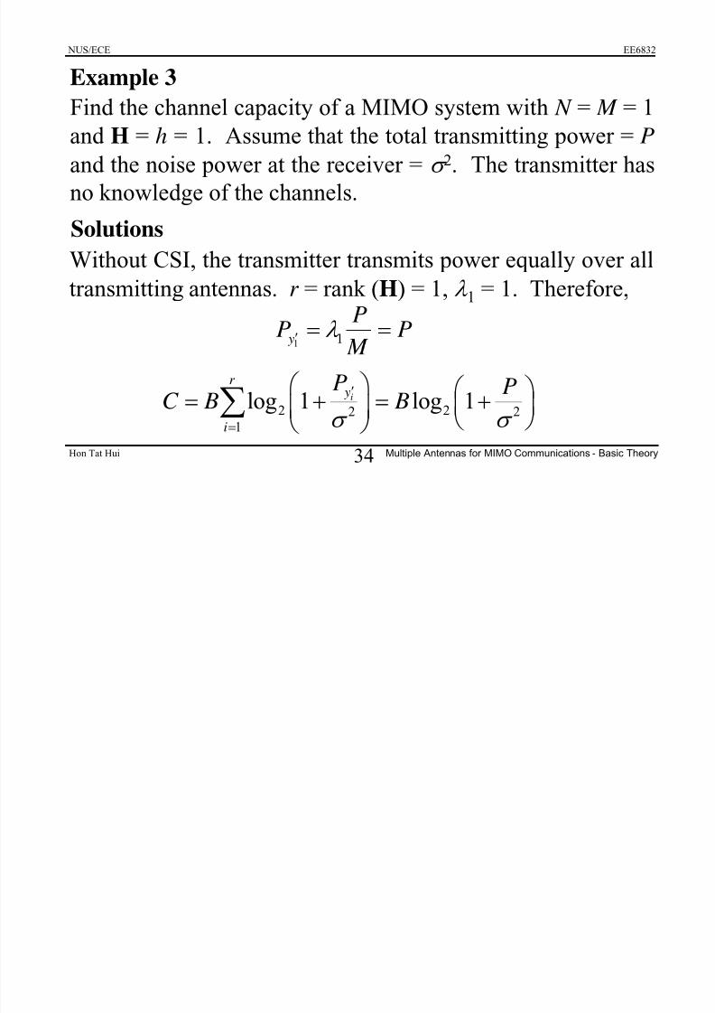
Example 3
Find the channel capacity of a MIMO system with N = M = 1
and H = h = 1. Assume that the total transmitting power = P
and the noise power at the receiver = 2. The transmitter has
no knowledge of the channels.
Solutions
Without CSI, the transmitter transmits power equally over alltransmitting antennas. r = rank (H) = 1, 1 = 1. Therefore,
2 22 21
log 1 log 1i
r y
i
P PC B B
1 1 y
PP P
8/13/2019 Lecture Notes-Multiple Antennas for MIMO Communications - Basic Theory
http://slidepdf.com/reader/full/lecture-notes-multiple-antennas-for-mimo-communications-basic-theory 35/48
Hon Tat Hui Multiple Antennas for MIMO Communications - Basic Theory
NUS/ECE EE6832
35
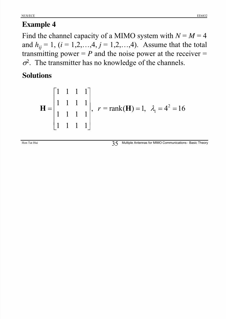
Example 4
Find the channel capacity of a MIMO system with N = M = 4
and hij = 1, (i = 1,2,…,4, j = 1,2,…,4). Assume that the total
transmitting power = P and the noise power at the receiver =
2. The transmitter has no knowledge of the channels.
Solutions
2
1
1 1 1 1
1 1 1 1, = rank( ) 1, 4 16
1 1 1 1
1 1 1 1
r
H H
8/13/2019 Lecture Notes-Multiple Antennas for MIMO Communications - Basic Theory
http://slidepdf.com/reader/full/lecture-notes-multiple-antennas-for-mimo-communications-basic-theory 36/48
Hon Tat Hui Multiple Antennas for MIMO Communications - Basic Theory
NUS/ECE EE6832
36
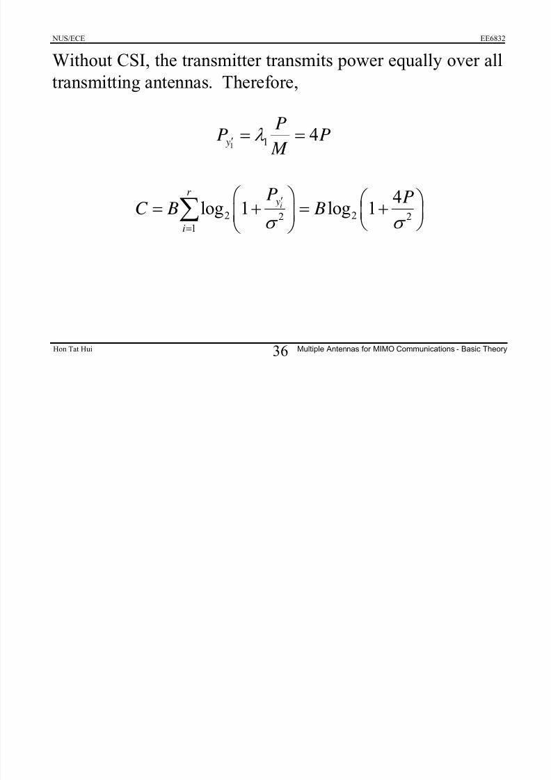
1 1 4 y
P
P P
2 22 21
4log 1 log 1
i
r y
i
P PC B B
Without CSI, the transmitter transmits power equally over all
transmitting antennas. Therefore,

8/13/2019 Lecture Notes-Multiple Antennas for MIMO Communications - Basic Theory
http://slidepdf.com/reader/full/lecture-notes-multiple-antennas-for-mimo-communications-basic-theory 37/48
Hon Tat Hui Multiple Antennas for MIMO Communications - Basic Theory
NUS/ECE EE6832
37
Example 5
The conditions are same as those in Example 4 but the
transmitter now knows the channel matrix H perfectly. Find
the channel capacity.
Solutions
2
1
1 1 1 1
1 1 1 1, = rank( ) 1, 4 16
1 1 1 1
1 1 1 1
r
H H
With knowledge of H, the transmitter can transmit power
along only one channel, i.e., the channel with eigenvalue 1.
8/13/2019 Lecture Notes-Multiple Antennas for MIMO Communications - Basic Theory
http://slidepdf.com/reader/full/lecture-notes-multiple-antennas-for-mimo-communications-basic-theory 38/48
Hon Tat Hui Multiple Antennas for MIMO Communications - Basic Theory
NUS/ECE EE6832
38
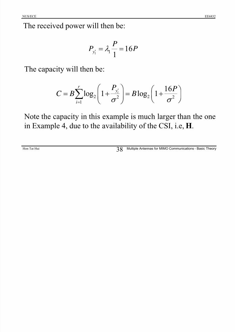
The received power will then be:
1 1 161
y
PP P
The capacity will then be:
2 22 21
16log 1 log 1i
r y
i
P PC B B
Note the capacity in this example is much larger than the onein Example 4, due to the availability of the CSI, i.e, H.
NUS/ECE EE6832

8/13/2019 Lecture Notes-Multiple Antennas for MIMO Communications - Basic Theory
http://slidepdf.com/reader/full/lecture-notes-multiple-antennas-for-mimo-communications-basic-theory 39/48
Hon Tat Hui Multiple Antennas for MIMO Communications - Basic Theory
NUS/ECE EE6832
39
Example 6
Find the channel capacity of a MIMO system with N = M = 4
and
Assume that the total transmitting power = P and the noise
power at the receiver = 2. The transmitter has no knowledge
of the channels.
1 0 0 00 1 0 0
0 0 1 0
0 0 0 1
H
NUS/ECE EE6832
8/13/2019 Lecture Notes-Multiple Antennas for MIMO Communications - Basic Theory
http://slidepdf.com/reader/full/lecture-notes-multiple-antennas-for-mimo-communications-basic-theory 40/48
Hon Tat Hui Multiple Antennas for MIMO Communications - Basic Theory
NUS/ECE EE6832
40
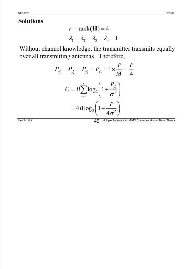
Solutions
1 2 3 4
= rank( ) 4
1
r
H
2 2
1
2 2
log 1
4 log 14
i
r y
i
PC B
P B
1 2 3 4 1 4 y y y y
P PP P P P
Without channel knowledge, the transmitter transmits equallyover all transmitting antennas. Therefore,
NUS/ECE EE6832
8/13/2019 Lecture Notes-Multiple Antennas for MIMO Communications - Basic Theory
http://slidepdf.com/reader/full/lecture-notes-multiple-antennas-for-mimo-communications-basic-theory 41/48
Hon Tat Hui Multiple Antennas for MIMO Communications - Basic Theory
NUS/ECE EE6832
41
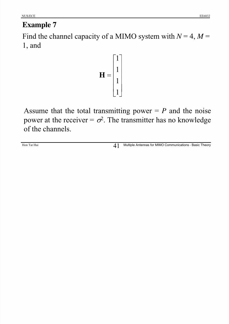
Example 7
Find the channel capacity of a MIMO system with N = 4, M =
1, and
Assume that the total transmitting power = P and the noise
power at the receiver = 2. The transmitter has no knowledge
of the channels.
11
1
1
H
NUS/ECE EE6832
8/13/2019 Lecture Notes-Multiple Antennas for MIMO Communications - Basic Theory
http://slidepdf.com/reader/full/lecture-notes-multiple-antennas-for-mimo-communications-basic-theory 42/48
Hon Tat Hui Multiple Antennas for MIMO Communications - Basic Theory
NUS/ECE EE6832
42
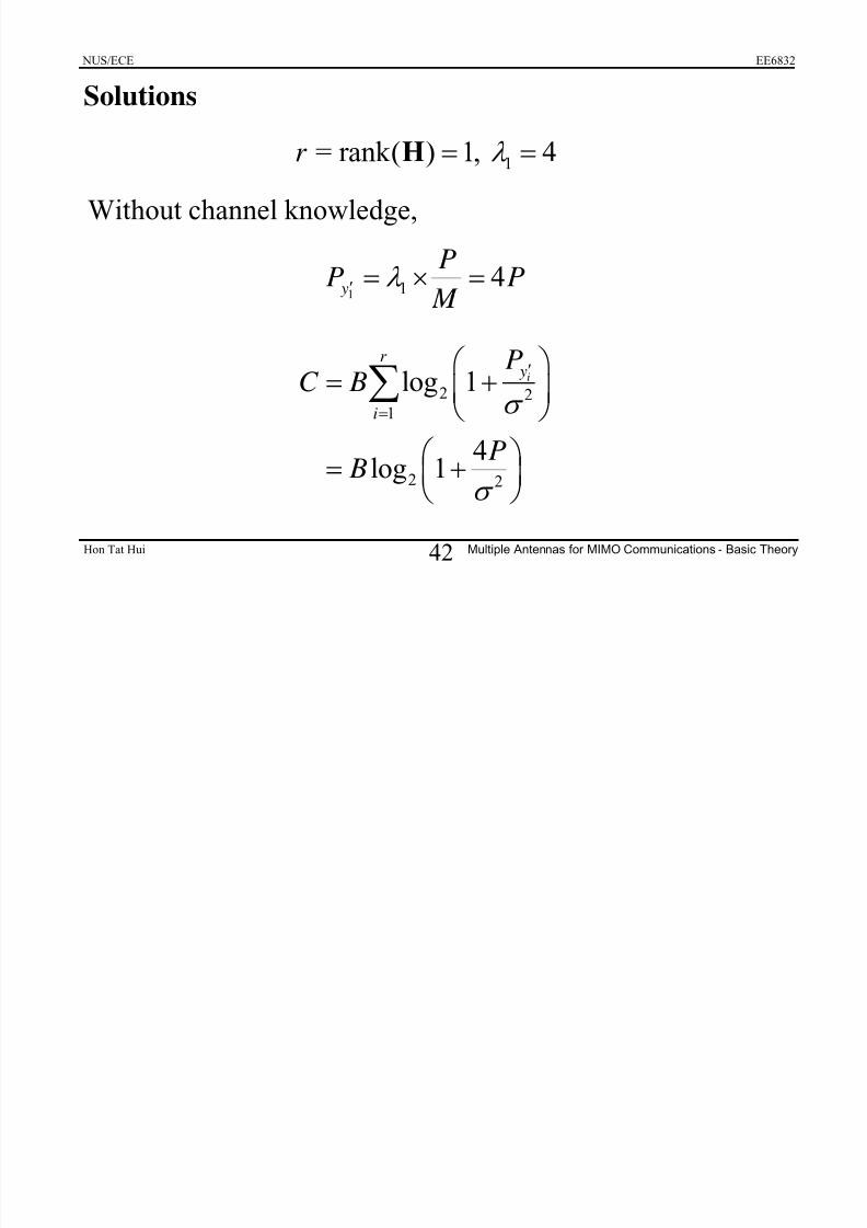
Solutions
1= rank( ) 1, 4r H
2 21
2 2
log 1
4log 1
i
r y
i
PC B
P B
1 1 4 y
PP P
Without channel knowledge,
NUS/ECE EE6832
8/13/2019 Lecture Notes-Multiple Antennas for MIMO Communications - Basic Theory
http://slidepdf.com/reader/full/lecture-notes-multiple-antennas-for-mimo-communications-basic-theory 43/48
Hon Tat Hui Multiple Antennas for MIMO Communications - Basic Theory
NUS/ECE EE6832
43
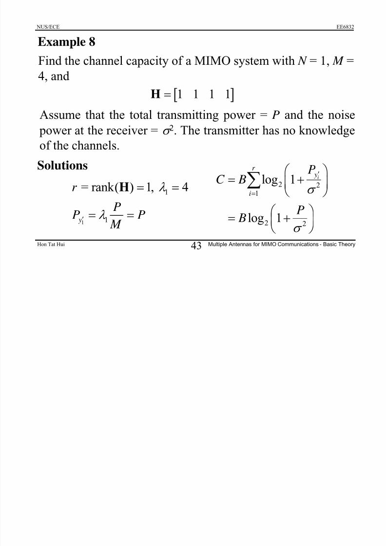
Example 8
Find the channel capacity of a MIMO system with N = 1, M =
4, and
Assume that the total transmitting power = P and the noise
power at the receiver = 2. The transmitter has no knowledge
of the channels.
1 1 1 1
H
Solutions
1
1
1
= rank( ) 1, 4
y
r
PP P
H 2 2
1
2 2
log 1
log 1
i
r y
i
PC B
P B
NUS/ECE EE6832
8/13/2019 Lecture Notes-Multiple Antennas for MIMO Communications - Basic Theory
http://slidepdf.com/reader/full/lecture-notes-multiple-antennas-for-mimo-communications-basic-theory 44/48
Hon Tat Hui Multiple Antennas for MIMO Communications - Basic Theory
NUS/ C 683
44
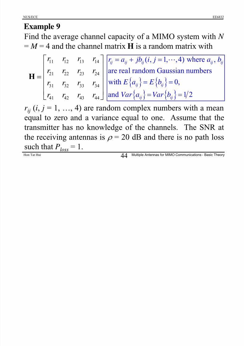
Example 9
Find the average channel capacity of a MIMO system with N
= M = 4 and the channel matrix H is a random matrix with
r ij (i, j = 1, …, 4) are random complex numbers with a mean
equal to zero and a variance equal to one. Assume that the
transmitter has no knowledge of the channels. The SNR at
the receiving antennas is = 20 dB and there is no path loss
such that Ploss = 1.
11 12 13 14
21 22 23 24
31 32 33 34
41 42 43 44
r r r r
r r r r
r r r r
r r r r
H
( , 1, ,4) where ,are real random Gaussian numbers
with 0,
and 1 2
ij ij ij ij ij
ij ij
ij ij
r a jb i j a b
E a E b
Var a Var b
NUS/ECE EE6832
8/13/2019 Lecture Notes-Multiple Antennas for MIMO Communications - Basic Theory
http://slidepdf.com/reader/full/lecture-notes-multiple-antennas-for-mimo-communications-basic-theory 45/48
Hon Tat Hui Multiple Antennas for MIMO Communications - Basic Theory45
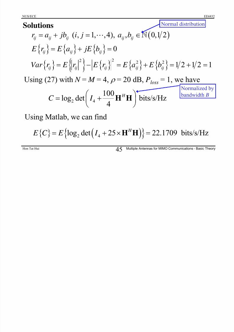
Solutions
Using (27) with N = M = 4, = 20 dB, Ploss = 1, we have
2 4
100log det bits/s/Hz
4
H C I
H H
22 2 2
( , 1, ,4), , 0,1 2
0
1 2 1 2 1
ij ij ij ij ij
ij ij ij
ij ij ij ij ij
r a jb i j a b
E r E a jE b
Var r E r E r E a E b
Normal distribution
Using Matlab, we can find
2 4log det 25 22.1709 bits/s/Hz H E C E I H H
Normalized by bandwidth B
NUS/ECE EE6832
8/13/2019 Lecture Notes-Multiple Antennas for MIMO Communications - Basic Theory
http://slidepdf.com/reader/full/lecture-notes-multiple-antennas-for-mimo-communications-basic-theory 46/48
Hon Tat Hui Multiple Antennas for MIMO Communications - Basic Theory46
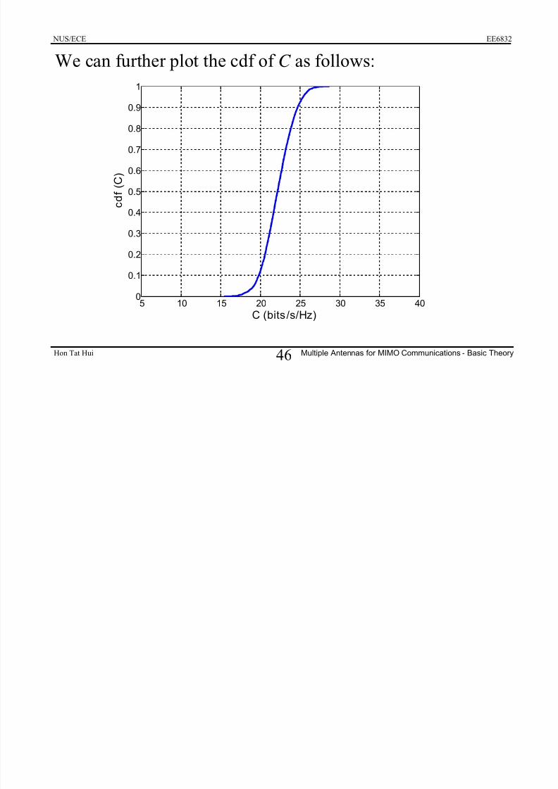
We can further plot the cdf of C as follows:
5 10 15 20 25 30 35 400
0.1
0.2
0.3
0.4
0.5
0.6
0.7
0.8
0.9
1
C (bits/s/Hz)
c d f ( C )
NUS/ECE EE6832
8/13/2019 Lecture Notes-Multiple Antennas for MIMO Communications - Basic Theory
http://slidepdf.com/reader/full/lecture-notes-multiple-antennas-for-mimo-communications-basic-theory 47/48
Hon Tat Hui Multiple Antennas for MIMO Communications - Basic Theory47
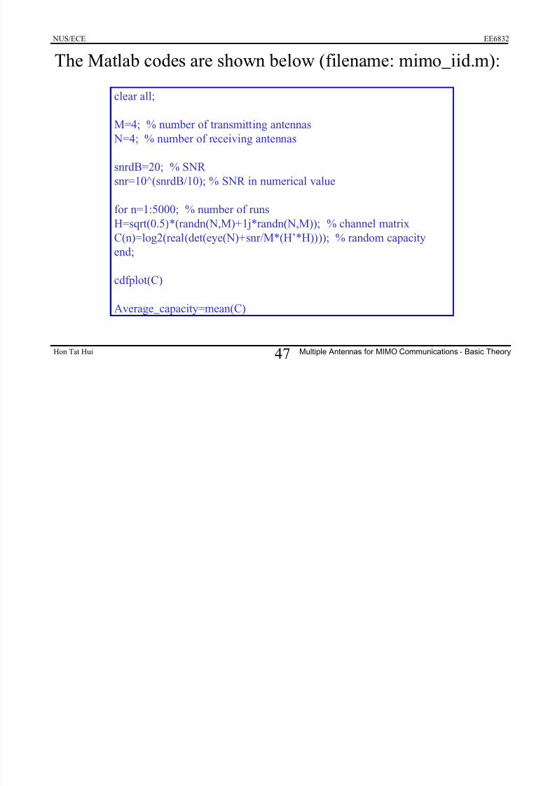
clear all;
M=4; % number of transmitting antennas
N=4; % number of receiving antennas
snrdB=20; % SNR
snr=10^(snrdB/10); % SNR in numerical value
for n=1:5000; % number of runsH=sqrt(0.5)*(randn(N,M)+1j*randn(N,M)); % channel matrix
C(n)=log2(real(det(eye(N)+snr/M*(H’*H)))); % random capacity
end;
cdfplot(C)
Average_capacity=mean(C)
The Matlab codes are shown below (filename: mimo_iid.m):
NUS/ECE EE6832
8/13/2019 Lecture Notes-Multiple Antennas for MIMO Communications - Basic Theory
http://slidepdf.com/reader/full/lecture-notes-multiple-antennas-for-mimo-communications-basic-theory 48/48
Hon Tat Hui Multiple Antennas for MIMO Communications - Basic Theory48
References:
[1] D. Gesbert, M. Shafi, D. Shiu, P. J. Smith, and A. Naguib, “From theory to practice: an overview of MIMO space–time coded wireless systems,” IEEE
Journal on Selected Areas in Communications, vol. 21, no. 3, pp. 281-302,
2003.
[2] E. Biglieri, R. Calderban, A. Constantinides, A. Goldsmith, A. Paulraj, and H.V. Poor, MIMO Wireless Communications, Cambridge University Press, 2007.
[3] F. G. Stremler, Introduction to Communication Systems, Addison-Wesley,
1982.
[4] R. Horn and C. Johnson, Matrix Analysis, Cambridge University Press, 1985.
[5] Branka Vucetic and Jinhong Yuan, Space-Time Coding, John Wiley & Sons
Ltd, 2003.