MIMO I: Spatial Diversity

COS 463: Wireless NetworksLecture 16

Kyle Jamieson

[Parts adapted from D. Halperin et al., T. Rappaport]

• Multiple-Input, Multiple-Output (MIMO) communications– Sends and receive more than one signal on different transmit

and receive antennas

• We’ve already seen frequency, time, spatial multiplexing in 463:

– MIMO is a more powerful way to multiplex wireless medium in space

– Transforms multipath propagation from an impediment to an advantage

2

What is MIMO, and why?

Many Uses of MIMO• At least three different ways to leverage space:

1. Spatial diversity: Send or receive redundant streams of information in parallel along multiple spatial paths– Increases reliability and range (unlikely that all paths will be

degraded simultaneously)

2. Spatial multiplexing: Send independent streams of information in parallel along multiple spatial paths– Increases rate, if we can avoid interference

3. Interference alignment: “Align” two streams of interference at a remote receiver, resulting in the impact of just one interference stream

MIMO-OFDM

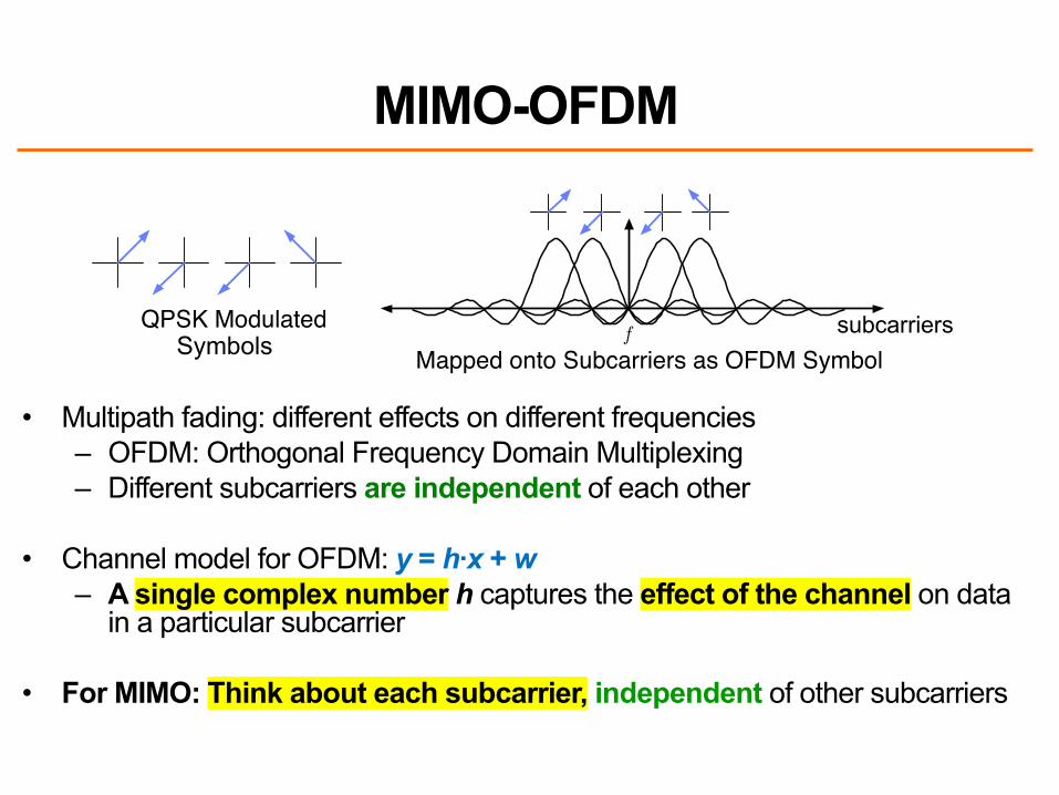
• Multipath fading: different effects on different frequencies– OFDM: Orthogonal Frequency Domain Multiplexing– Different subcarriers are independent of each other

• Channel model for OFDM: y = h∙x + w– A single complex number h captures the effect of the channel on data

in a particular subcarrier

• For MIMO: Think about each subcarrier, independent of other subcarriers

(5) QPSK Modulatedf

(6) Mapped onto Subcarriers as OFDM Symbol

Figure 1: A graphical view of the OFDM encoding process for the 18 Mbps rate (QPSK, 3/4) of 802.11a.The data bits (0) are encoded by a rate-1/2 convolutional code (1) and then optionally punctured by droppingcertain bits for higher coding rates (here, 3/4) that send fewer redundant bits (2). The remaining bits are in-terleaved (3) to spread the redundancy across subcarriers and protect against frequency-selective fades. Thesebits are grouped into symbols (4) based on the modulation (QPSK encodes 2 bits per symbol), modulated (5),and finally mapped onto the di↵erent subcarriers to form an OFDM symbol (6).

h11

h12

h11

h12y = x2

Tx Rx

y = xx

1

(a) Receive diversity

h11

h21

h11 h21

Tx Rx

x

x

( + ) xy =

y

(b) Transmit diversity

x1

x2

h11

h12h21

h22

h11x1 h21x2

h12x1 h22x2y2 = +

Tx Rx

y = 1 +

(c) Spatial multiplexing

Figure 2: Using some of the transmit/receive antennas in an example 2x2 system to exploit diversity andmultiplexing gain. xi and yi represent transmitted and received signals. The channel gain hij is a complexnumber indicating a signal’s attenuated amplitude and phase shift over the channel between the ith transmitantenna and the jth receive antenna. The received signals yi will additionally include thermal RF noise.

modulation sending more bits per symbol and being usedwhen there is a higher SNR. There are minor di↵erences be-tween 802.11a/g and 802.11n. In 802.11a/g there are 48 datasubcarriers, 4 pilot tones for control, and 6 unused guardsubcarriers at each edge of the channel. In 802.11n, thereare only 4 guard subcarriers at each edge of the channel, andtwo adjacent 20 MHz channels can be merged into a single40 MHz channel.

The beauty of OFDM is that it divides the channel in away that is both computationally and spectrally e�cient.High aggregate data rates can be achieved, while the en-coding and decoding on di↵erent subcarriers can use sharedhardware components. More relevant to our point here, how-ever, is that OFDM transforms a single large channel intomany relatively independently faded channels. This is be-cause multi-path fading is frequency selective, so the di↵er-ent subcarriers will experience di↵erent fades. Some adja-cent subcarriers may be faded in a similar way, but the fadingfor more distant subcarriers is often uncorrelated. Dividingthe channel also increases the symbol time per channel, sincemany slow symbols will be sent in parallel instead of manyfast symbols in sequence. This adds time diversity becausethe channel is more likely to average out fades over a longerperiod of time.

802.11 makes use of the frequency diversity provided byOFDM by coding across the data carried on the subcarriers.This uses a fraction of them for redundant information thatcan later be used to correct errors that occur when fadingreduces the SNR on some of the subcarriers. First, a con-

volutional code of rate 1/2 adds redundant information. Itis then punctured [3] by removing bits as needed to supportcoding rates of 2/3 and 3/4, plus 5/6 for 802.11n. At a rateof 3/4, for example, a quarter of the data on the subcarriersis redundant. An alternative LDPC (Low-Density Parity-Check) code with slightly better performance can also beused for 802.11n. Figure 1 presents a pictorial overview ofthe OFDM encoding process.

The net e↵ect of OFDM plus coding is to provide consis-tently good 802.11 performance despite significant variabil-ity in the wireless signal due to multi-path fading.

3. SPATIAL DIVERSITYIn this section we look at spatial diversity techniques that

can be applied at the receiver and at the transmitter. Addingmultiple antennas to an 802.11n receiver or transmitter pro-vides a new set of independently faded paths, even if theantennas are separated by only a few centimeters. Thisadds spatial diversity to the system, which can be exploitedto improve resilience to fades. There is also a power gainfrom multiple receive antennas because, everything else be-ing equal, two receive antennas will receive twice the signal.These factors combine to improve performance at a givendistance, and hence increase range.

3.1 Receive Diversity TechniquesConsider the arrangement in Figure 2(a). One transmit

antenna at a node is sending to two receive antennas at a

subcarriersSymbols

1. Today: Diversity in Space– Receive Diversity– Transmit Diversity

2. Next time: Multiplexing in Space

3. Next time: Interference Alignment

5

Plan

1. Multi-Antenna Access Points (APs), especially 802.11n,ac:

2. Multiple APs cooperating with each other:

3. Distributed Antenna systems, separating antenna from AP:

6

Path Diversity: Motivation

Wired backhaul

AP

Antenna 1Antenna 2

Coaxial / Fiberbackhaul

• Typical outdoor multipath propagation environment, channel h

• On one link each subcarrier’s power level experiences Rayleigh fading:

7

Review: Fast Fading

! "

8

Uncorrelated Rayleigh Fading• Suppose two antennas, separated by distance d12

• Channels from each to a distant thirdantenna (h13, h23) can be uncorrelated– Fading happens at different times with no bias for a simultaneous fade

!" #, !# #

• Channels from each antenna (h13, h23) to a third antenna– Channels are uncorrelated when !"# >≈ &.()– Channels correlated, fade together when !"# <≈ )

• This correlation distance depends on the radio environment around the pair of antennas– Increases, e.g., atop cellular phone tower

9

When is Fading Uncorrelated, and Why?

≫ , !"#

1. Today: Diversity in Space– Receive Diversity

• Selection Diversity• Maximal Ratio Combining

– Transmit Diversity

2. Next time: Multiplexing in Space

3. Next time: Interference Alignment

10

Plan

• One transmit antenna sends a symbol to two receive antennas– Receive diversity, or Single-Input, Multi-Output (SIMO)

• Each receive antenna gets own copy of transmitted signal via – Different path– Potentially different channel

Channel Model for Receive Diversity

n2

y2=2e-iπ/6x

rotate, scale by 2/p

13

rotate, scale by 3/p

13

�

9/p

13

4/p

13

p13

x

n expected 1

y1=3ei3π/4x

n1

Figure 3: MRC operation on a sample channel. The channel gains are ~h = h3ei3⇡/4

, 2e�i⇡/6i, with Gaussian

noise ~n = hn1, n2i of expected power 1. The antennas have respective SNRs of 9 and 4. To implement MRC,

the receiver multiplies the received signal ~y = ~hx + ~n by the unit vector ~h⇤/||~h||, where ~h

⇤ denotes the complex

conjugate of ~h. This operation scales each antenna’s signal by its magnitude, and rotates the signals intothe same phase reference before adding them. (For graphical clarity, we depict the common phase vertically,rather than at 0). The resulting sum has magnitude

p13, and expected noise power 1 because the scaling is

normalized. Thus, by coherently combining received signals from di↵erent antennas, the MRC output hasthe expected SNR of 13. In systems with OFDM, MRC is performed separately for each subcarrier.

second node. This is known as a 1x2 system. Real systemsmay have more than two receive antennas, but two will suf-fice for our explanation. With this setup, each receive an-tenna receives a copy of the transmitted signal modified bythe channel between the transmitter and itself. The chan-nel gains hij are complex numbers that represent both theamplitude attenuation over the channel as well as the path-dependent phase shift (see Figure 3 for a graphical example).The receiver measures the channel gains based on trainingfields in the packet preamble. Note that the gains di↵er foreach subcarrier (in frequency-selective fading) as well as foreach antenna. The question now is how to combine the tworeceived signals to make best use of them.

We consider two diversity techniques to show the extremes.The simplest method is to use the antenna with the strongestsignal (hence the largest SNR) to receive the packet and ig-nore the others. We will call this method SEL, for selection

combining. This is essentially what is done by 802.11a/g APswith multiple antennas. It helps with reliability, becauseboth signals are unlikely to be bad, but it wastes perfectlygood received power at the antennas that are not chosen.

The better method is to add the signals from the twoantennas together. However, this cannot be done by simplysuperimposing their signals, or we will have just recreatedthe e↵ects of multi-path fading. Rather, the signals shouldeach be delayed until they are in the same phase; then, thepower in the signals will combine coherently. To do this,the receiver needs a dedicated RF chain for each antenna toprocess the signals. This increases the hardware complexityand power consumption, but yields better performance.

As a twist in the above, the signals are also weighted bytheir SNRs. This gives less weight to a signal that has alarger fraction of noise, so that the e↵ects of the noise are notamplified. The result is maximal-ratio combining, or MRC.MRC is known to be optimal (it maximizes SIMO capacity),and produces an SNR that is the sum of the componentSNRs. Note that in frequency-selective fading, this processis performed di↵erently for each subcarrier according to itsspecific channel gains.

Figure 3 depicts MRC operation graphically for a 1x2channel. In this example, the two channel gains have magni-

-25

-20

-15

-10

-5

0

-20 -10 0 10 20

No

rma

lize

d p

ow

er

(dB

)

Subcarrier index

AC

B and SELAB (MRC)

ABC (MRC)

Figure 4: Frequency-selective fading over testbedlinks: the figure shows, for an example 5.2 GHz link,the received power measured on each subcarrier forindividual antennas and under SEL and MRC diver-sity, normalized to the strongest subcarrier power.

tudes of 3 and 2. With expected noise power 1, these gainscorrespond to SNRs of 9 and 4, given that a signal’s power isthe square of its magnitude. The MRC receiver scales eachantenna’s signal by its magnitude, normalized to the total;delays the signals to a common phase reference; and thenadds them. The result has magnitude

p13, and the normal-

ized weighted sum of noise still has expected power 1. Thecombined signal thus has a resulting sum SNR of 13.

As an example of how MRC and SEL work in 802.11, con-sider Figure 4. This figure shows the wireless signal strengthof each subcarrier using three antennas for a real 802.11n linkin our indoor wireless testbed. The subcarrier strengths aremeasured in decibels normalized to the strongest subcarrierstrength. This figure gives a much more detailed view thanmetrics such as the RSSI (Received Signal Strength Indi-cation) for a link, which gives only the sum of the signalstrength over all subcarriers.

For each antenna labeled A, B, or C, the signal variesover the channel, changing gradually from one subcarrier

Figure 1: A graphical view of the OFDM encoding process for the 18 Mbps rate (QPSK, 3/4) of 802.11a.The data bits (0) are encoded by a rate-1/2 convolutional code (1) and then optionally punctured by droppingcertain bits for higher coding rates (here, 3/4) that send fewer redundant bits (2). The remaining bits are in-terleaved (3) to spread the redundancy across subcarriers and protect against frequency-selective fades. Thesebits are grouped into symbols (4) based on the modulation (QPSK encodes 2 bits per symbol), modulated (5),and finally mapped onto the di↵erent subcarriers to form an OFDM symbol (6).

h11

h12

h11

h12y = x2

Tx Rx

y = xx

1

(a) Receive diversity

h11

h21

h11 h21

Tx Rx

x

x

( + ) xy =

y

(b) Transmit diversity

x1

x2

h11

h12h21

h22

h11x1 h21x2

h12x1 h22x2y2 = +

Tx Rx

y = 1 +

(c) Spatial multiplexing

Figure 2: Using some of the transmit/receive antennas in an example 2x2 system to exploit diversity andmultiplexing gain. xi and yi represent transmitted and received signals. The channel gain hij is a complexnumber indicating a signal’s attenuated amplitude and phase shift over the channel between the ith transmitantenna and the jth receive antenna. The received signals yi will additionally include thermal RF noise.

modulation sending more bits per symbol and being usedwhen there is a higher SNR. There are minor di↵erences be-tween 802.11a/g and 802.11n. In 802.11a/g there are 48 datasubcarriers, 4 pilot tones for control, and 6 unused guardsubcarriers at each edge of the channel. In 802.11n, thereare only 4 guard subcarriers at each edge of the channel, andtwo adjacent 20 MHz channels can be merged into a single40 MHz channel.

The beauty of OFDM is that it divides the channel in away that is both computationally and spectrally e�cient.High aggregate data rates can be achieved, while the en-coding and decoding on di↵erent subcarriers can use sharedhardware components. More relevant to our point here, how-ever, is that OFDM transforms a single large channel intomany relatively independently faded channels. This is be-cause multi-path fading is frequency selective, so the di↵er-ent subcarriers will experience di↵erent fades. Some adja-cent subcarriers may be faded in a similar way, but the fadingfor more distant subcarriers is often uncorrelated. Dividingthe channel also increases the symbol time per channel, sincemany slow symbols will be sent in parallel instead of manyfast symbols in sequence. This adds time diversity becausethe channel is more likely to average out fades over a longerperiod of time.

802.11 makes use of the frequency diversity provided byOFDM by coding across the data carried on the subcarriers.This uses a fraction of them for redundant information thatcan later be used to correct errors that occur when fadingreduces the SNR on some of the subcarriers. First, a con-

volutional code of rate 1/2 adds redundant information. Itis then punctured [3] by removing bits as needed to supportcoding rates of 2/3 and 3/4, plus 5/6 for 802.11n. At a rateof 3/4, for example, a quarter of the data on the subcarriersis redundant. An alternative LDPC (Low-Density Parity-Check) code with slightly better performance can also beused for 802.11n. Figure 1 presents a pictorial overview ofthe OFDM encoding process.

The net e↵ect of OFDM plus coding is to provide consis-tently good 802.11 performance despite significant variabil-ity in the wireless signal due to multi-path fading.

3. SPATIAL DIVERSITYIn this section we look at spatial diversity techniques that

can be applied at the receiver and at the transmitter. Addingmultiple antennas to an 802.11n receiver or transmitter pro-vides a new set of independently faded paths, even if theantennas are separated by only a few centimeters. Thisadds spatial diversity to the system, which can be exploitedto improve resilience to fades. There is also a power gainfrom multiple receive antennas because, everything else be-ing equal, two receive antennas will receive twice the signal.These factors combine to improve performance at a givendistance, and hence increase range.

3.1 Receive Diversity TechniquesConsider the arrangement in Figure 2(a). One transmit

antenna at a node is sending to two receive antennas at a

Receive antenna 1h1

h2Receive antenna 2

x

Selection Diversity

• Two receive antennas share one receiving radio

• Chooses the antenna with stronger signal, sends that to the radio– Helps reliability (both unlikely bad)– Wastes received signal from other antenna(s)

n2

y2=2e-iπ/6x

rotate, scale by 2/p

13

rotate, scale by 3/p

13

�

9/p

13

4/p

13

p13

x

n expected 1

y1=3ei3π/4x

n1

Figure 3: MRC operation on a sample channel. The channel gains are ~h = h3ei3⇡/4

, 2e�i⇡/6i, with Gaussian

noise ~n = hn1, n2i of expected power 1. The antennas have respective SNRs of 9 and 4. To implement MRC,

the receiver multiplies the received signal ~y = ~hx + ~n by the unit vector ~h⇤/||~h||, where ~h

⇤ denotes the complex

conjugate of ~h. This operation scales each antenna’s signal by its magnitude, and rotates the signals intothe same phase reference before adding them. (For graphical clarity, we depict the common phase vertically,rather than at 0). The resulting sum has magnitude

p13, and expected noise power 1 because the scaling is

normalized. Thus, by coherently combining received signals from di↵erent antennas, the MRC output hasthe expected SNR of 13. In systems with OFDM, MRC is performed separately for each subcarrier.

second node. This is known as a 1x2 system. Real systemsmay have more than two receive antennas, but two will suf-fice for our explanation. With this setup, each receive an-tenna receives a copy of the transmitted signal modified bythe channel between the transmitter and itself. The chan-nel gains hij are complex numbers that represent both theamplitude attenuation over the channel as well as the path-dependent phase shift (see Figure 3 for a graphical example).The receiver measures the channel gains based on trainingfields in the packet preamble. Note that the gains di↵er foreach subcarrier (in frequency-selective fading) as well as foreach antenna. The question now is how to combine the tworeceived signals to make best use of them.

We consider two diversity techniques to show the extremes.The simplest method is to use the antenna with the strongestsignal (hence the largest SNR) to receive the packet and ig-nore the others. We will call this method SEL, for selection

combining. This is essentially what is done by 802.11a/g APswith multiple antennas. It helps with reliability, becauseboth signals are unlikely to be bad, but it wastes perfectlygood received power at the antennas that are not chosen.

The better method is to add the signals from the twoantennas together. However, this cannot be done by simplysuperimposing their signals, or we will have just recreatedthe e↵ects of multi-path fading. Rather, the signals shouldeach be delayed until they are in the same phase; then, thepower in the signals will combine coherently. To do this,the receiver needs a dedicated RF chain for each antenna toprocess the signals. This increases the hardware complexityand power consumption, but yields better performance.

As a twist in the above, the signals are also weighted bytheir SNRs. This gives less weight to a signal that has alarger fraction of noise, so that the e↵ects of the noise are notamplified. The result is maximal-ratio combining, or MRC.MRC is known to be optimal (it maximizes SIMO capacity),and produces an SNR that is the sum of the componentSNRs. Note that in frequency-selective fading, this processis performed di↵erently for each subcarrier according to itsspecific channel gains.

Figure 3 depicts MRC operation graphically for a 1x2channel. In this example, the two channel gains have magni-

-25

-20

-15

-10

-5

0

-20 -10 0 10 20

No

rma

lize

d p

ow

er

(dB

)

Subcarrier index

AC

B and SELAB (MRC)

ABC (MRC)

Figure 4: Frequency-selective fading over testbedlinks: the figure shows, for an example 5.2 GHz link,the received power measured on each subcarrier forindividual antennas and under SEL and MRC diver-sity, normalized to the strongest subcarrier power.

tudes of 3 and 2. With expected noise power 1, these gainscorrespond to SNRs of 9 and 4, given that a signal’s power isthe square of its magnitude. The MRC receiver scales eachantenna’s signal by its magnitude, normalized to the total;delays the signals to a common phase reference; and thenadds them. The result has magnitude

p13, and the normal-

ized weighted sum of noise still has expected power 1. Thecombined signal thus has a resulting sum SNR of 13.

As an example of how MRC and SEL work in 802.11, con-sider Figure 4. This figure shows the wireless signal strengthof each subcarrier using three antennas for a real 802.11n linkin our indoor wireless testbed. The subcarrier strengths aremeasured in decibels normalized to the strongest subcarrierstrength. This figure gives a much more detailed view thanmetrics such as the RSSI (Received Signal Strength Indi-cation) for a link, which gives only the sum of the signalstrength over all subcarriers.

For each antenna labeled A, B, or C, the signal variesover the channel, changing gradually from one subcarrier

Radio

Figure 1: A graphical view of the OFDM encoding process for the 18 Mbps rate (QPSK, 3/4) of 802.11a.The data bits (0) are encoded by a rate-1/2 convolutional code (1) and then optionally punctured by droppingcertain bits for higher coding rates (here, 3/4) that send fewer redundant bits (2). The remaining bits are in-terleaved (3) to spread the redundancy across subcarriers and protect against frequency-selective fades. Thesebits are grouped into symbols (4) based on the modulation (QPSK encodes 2 bits per symbol), modulated (5),and finally mapped onto the di↵erent subcarriers to form an OFDM symbol (6).

h11

h12

h11

h12y = x2

Tx Rx

y = xx

1

(a) Receive diversity

h11

h21

h11 h21

Tx Rx

x

x

( + ) xy =

y

(b) Transmit diversity

x1

x2

h11

h12h21

h22

h11x1 h21x2

h12x1 h22x2y2 = +

Tx Rx

y = 1 +

(c) Spatial multiplexing

Figure 2: Using some of the transmit/receive antennas in an example 2x2 system to exploit diversity andmultiplexing gain. xi and yi represent transmitted and received signals. The channel gain hij is a complexnumber indicating a signal’s attenuated amplitude and phase shift over the channel between the ith transmitantenna and the jth receive antenna. The received signals yi will additionally include thermal RF noise.

modulation sending more bits per symbol and being usedwhen there is a higher SNR. There are minor di↵erences be-tween 802.11a/g and 802.11n. In 802.11a/g there are 48 datasubcarriers, 4 pilot tones for control, and 6 unused guardsubcarriers at each edge of the channel. In 802.11n, thereare only 4 guard subcarriers at each edge of the channel, andtwo adjacent 20 MHz channels can be merged into a single40 MHz channel.

The beauty of OFDM is that it divides the channel in away that is both computationally and spectrally e�cient.High aggregate data rates can be achieved, while the en-coding and decoding on di↵erent subcarriers can use sharedhardware components. More relevant to our point here, how-ever, is that OFDM transforms a single large channel intomany relatively independently faded channels. This is be-cause multi-path fading is frequency selective, so the di↵er-ent subcarriers will experience di↵erent fades. Some adja-cent subcarriers may be faded in a similar way, but the fadingfor more distant subcarriers is often uncorrelated. Dividingthe channel also increases the symbol time per channel, sincemany slow symbols will be sent in parallel instead of manyfast symbols in sequence. This adds time diversity becausethe channel is more likely to average out fades over a longerperiod of time.

802.11 makes use of the frequency diversity provided byOFDM by coding across the data carried on the subcarriers.This uses a fraction of them for redundant information thatcan later be used to correct errors that occur when fadingreduces the SNR on some of the subcarriers. First, a con-

volutional code of rate 1/2 adds redundant information. Itis then punctured [3] by removing bits as needed to supportcoding rates of 2/3 and 3/4, plus 5/6 for 802.11n. At a rateof 3/4, for example, a quarter of the data on the subcarriersis redundant. An alternative LDPC (Low-Density Parity-Check) code with slightly better performance can also beused for 802.11n. Figure 1 presents a pictorial overview ofthe OFDM encoding process.

The net e↵ect of OFDM plus coding is to provide consis-tently good 802.11 performance despite significant variabil-ity in the wireless signal due to multi-path fading.

3. SPATIAL DIVERSITYIn this section we look at spatial diversity techniques that

can be applied at the receiver and at the transmitter. Addingmultiple antennas to an 802.11n receiver or transmitter pro-vides a new set of independently faded paths, even if theantennas are separated by only a few centimeters. Thisadds spatial diversity to the system, which can be exploitedto improve resilience to fades. There is also a power gainfrom multiple receive antennas because, everything else be-ing equal, two receive antennas will receive twice the signal.These factors combine to improve performance at a givendistance, and hence increase range.

3.1 Receive Diversity TechniquesConsider the arrangement in Figure 2(a). One transmit

antenna at a node is sending to two receive antennas at a

h1

h2Select strongerx

Rx 1

Rx 2

ECE 5325/6325 Spring 2010 76

Figure 32: Rappaport Figure 7.11, the impact of selection combining.

13

Selection Diversity:Performance Improvement

• In general, might have M receive antennas (average SNR Γ)– !": SNR of the i th receive antenna

• Probability selected SNR is less than some threshold γ:– Pr !%,⋯ , !( ≤ γ = Pr !" ≤ γ (

• One more “9” of reliability per additional selection branch

ß lower threshold SNR

Probability (%) that Selected Antenna’s SNR Exceeds Threshold γ

Higher probability (better) ↓

Leveraging All Receive Antennas

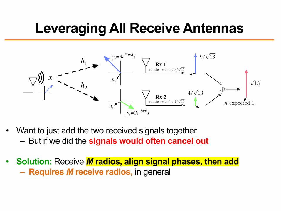
• Want to just add the two received signals together– But if we did the signals would often cancel out

• Solution: Receive M radios, align signal phases, then add– Requires M receive radios, in general

n2

y2=2e-iπ/6x

rotate, scale by 2/p

13

rotate, scale by 3/p

13

�

9/p

13

4/p

13

p13

x

n expected 1

y1=3ei3π/4x

n1

Figure 3: MRC operation on a sample channel. The channel gains are ~h = h3ei3⇡/4

, 2e�i⇡/6i, with Gaussian

noise ~n = hn1, n2i of expected power 1. The antennas have respective SNRs of 9 and 4. To implement MRC,

the receiver multiplies the received signal ~y = ~hx + ~n by the unit vector ~h⇤/||~h||, where ~h

⇤ denotes the complex

conjugate of ~h. This operation scales each antenna’s signal by its magnitude, and rotates the signals intothe same phase reference before adding them. (For graphical clarity, we depict the common phase vertically,rather than at 0). The resulting sum has magnitude

p13, and expected noise power 1 because the scaling is

normalized. Thus, by coherently combining received signals from di↵erent antennas, the MRC output hasthe expected SNR of 13. In systems with OFDM, MRC is performed separately for each subcarrier.

second node. This is known as a 1x2 system. Real systemsmay have more than two receive antennas, but two will suf-fice for our explanation. With this setup, each receive an-tenna receives a copy of the transmitted signal modified bythe channel between the transmitter and itself. The chan-nel gains hij are complex numbers that represent both theamplitude attenuation over the channel as well as the path-dependent phase shift (see Figure 3 for a graphical example).The receiver measures the channel gains based on trainingfields in the packet preamble. Note that the gains di↵er foreach subcarrier (in frequency-selective fading) as well as foreach antenna. The question now is how to combine the tworeceived signals to make best use of them.

We consider two diversity techniques to show the extremes.The simplest method is to use the antenna with the strongestsignal (hence the largest SNR) to receive the packet and ig-nore the others. We will call this method SEL, for selection

combining. This is essentially what is done by 802.11a/g APswith multiple antennas. It helps with reliability, becauseboth signals are unlikely to be bad, but it wastes perfectlygood received power at the antennas that are not chosen.

The better method is to add the signals from the twoantennas together. However, this cannot be done by simplysuperimposing their signals, or we will have just recreatedthe e↵ects of multi-path fading. Rather, the signals shouldeach be delayed until they are in the same phase; then, thepower in the signals will combine coherently. To do this,the receiver needs a dedicated RF chain for each antenna toprocess the signals. This increases the hardware complexityand power consumption, but yields better performance.

As a twist in the above, the signals are also weighted bytheir SNRs. This gives less weight to a signal that has alarger fraction of noise, so that the e↵ects of the noise are notamplified. The result is maximal-ratio combining, or MRC.MRC is known to be optimal (it maximizes SIMO capacity),and produces an SNR that is the sum of the componentSNRs. Note that in frequency-selective fading, this processis performed di↵erently for each subcarrier according to itsspecific channel gains.

Figure 3 depicts MRC operation graphically for a 1x2channel. In this example, the two channel gains have magni-

-25

-20

-15

-10

-5

0

-20 -10 0 10 20

No

rma

lize

d p

ow

er

(dB

)

Subcarrier index

AC

B and SELAB (MRC)

ABC (MRC)

Figure 4: Frequency-selective fading over testbedlinks: the figure shows, for an example 5.2 GHz link,the received power measured on each subcarrier forindividual antennas and under SEL and MRC diver-sity, normalized to the strongest subcarrier power.

tudes of 3 and 2. With expected noise power 1, these gainscorrespond to SNRs of 9 and 4, given that a signal’s power isthe square of its magnitude. The MRC receiver scales eachantenna’s signal by its magnitude, normalized to the total;delays the signals to a common phase reference; and thenadds them. The result has magnitude

p13, and the normal-

ized weighted sum of noise still has expected power 1. Thecombined signal thus has a resulting sum SNR of 13.

As an example of how MRC and SEL work in 802.11, con-sider Figure 4. This figure shows the wireless signal strengthof each subcarrier using three antennas for a real 802.11n linkin our indoor wireless testbed. The subcarrier strengths aremeasured in decibels normalized to the strongest subcarrierstrength. This figure gives a much more detailed view thanmetrics such as the RSSI (Received Signal Strength Indi-cation) for a link, which gives only the sum of the signalstrength over all subcarriers.

For each antenna labeled A, B, or C, the signal variesover the channel, changing gradually from one subcarrier

Figure 1: A graphical view of the OFDM encoding process for the 18 Mbps rate (QPSK, 3/4) of 802.11a.The data bits (0) are encoded by a rate-1/2 convolutional code (1) and then optionally punctured by droppingcertain bits for higher coding rates (here, 3/4) that send fewer redundant bits (2). The remaining bits are in-terleaved (3) to spread the redundancy across subcarriers and protect against frequency-selective fades. Thesebits are grouped into symbols (4) based on the modulation (QPSK encodes 2 bits per symbol), modulated (5),and finally mapped onto the di↵erent subcarriers to form an OFDM symbol (6).

h11

h12

h11

h12y = x2

Tx Rx

y = xx

1

(a) Receive diversity

h11

h21

h11 h21

Tx Rx

x

x

( + ) xy =

y

(b) Transmit diversity

x1

x2

h11

h12h21

h22

h11x1 h21x2

h12x1 h22x2y2 = +

Tx Rx

y = 1 +

(c) Spatial multiplexing

Figure 2: Using some of the transmit/receive antennas in an example 2x2 system to exploit diversity andmultiplexing gain. xi and yi represent transmitted and received signals. The channel gain hij is a complexnumber indicating a signal’s attenuated amplitude and phase shift over the channel between the ith transmitantenna and the jth receive antenna. The received signals yi will additionally include thermal RF noise.

modulation sending more bits per symbol and being usedwhen there is a higher SNR. There are minor di↵erences be-tween 802.11a/g and 802.11n. In 802.11a/g there are 48 datasubcarriers, 4 pilot tones for control, and 6 unused guardsubcarriers at each edge of the channel. In 802.11n, thereare only 4 guard subcarriers at each edge of the channel, andtwo adjacent 20 MHz channels can be merged into a single40 MHz channel.

The beauty of OFDM is that it divides the channel in away that is both computationally and spectrally e�cient.High aggregate data rates can be achieved, while the en-coding and decoding on di↵erent subcarriers can use sharedhardware components. More relevant to our point here, how-ever, is that OFDM transforms a single large channel intomany relatively independently faded channels. This is be-cause multi-path fading is frequency selective, so the di↵er-ent subcarriers will experience di↵erent fades. Some adja-cent subcarriers may be faded in a similar way, but the fadingfor more distant subcarriers is often uncorrelated. Dividingthe channel also increases the symbol time per channel, sincemany slow symbols will be sent in parallel instead of manyfast symbols in sequence. This adds time diversity becausethe channel is more likely to average out fades over a longerperiod of time.

802.11 makes use of the frequency diversity provided byOFDM by coding across the data carried on the subcarriers.This uses a fraction of them for redundant information thatcan later be used to correct errors that occur when fadingreduces the SNR on some of the subcarriers. First, a con-

volutional code of rate 1/2 adds redundant information. Itis then punctured [3] by removing bits as needed to supportcoding rates of 2/3 and 3/4, plus 5/6 for 802.11n. At a rateof 3/4, for example, a quarter of the data on the subcarriersis redundant. An alternative LDPC (Low-Density Parity-Check) code with slightly better performance can also beused for 802.11n. Figure 1 presents a pictorial overview ofthe OFDM encoding process.

The net e↵ect of OFDM plus coding is to provide consis-tently good 802.11 performance despite significant variabil-ity in the wireless signal due to multi-path fading.

3. SPATIAL DIVERSITYIn this section we look at spatial diversity techniques that

can be applied at the receiver and at the transmitter. Addingmultiple antennas to an 802.11n receiver or transmitter pro-vides a new set of independently faded paths, even if theantennas are separated by only a few centimeters. Thisadds spatial diversity to the system, which can be exploitedto improve resilience to fades. There is also a power gainfrom multiple receive antennas because, everything else be-ing equal, two receive antennas will receive twice the signal.These factors combine to improve performance at a givendistance, and hence increase range.

3.1 Receive Diversity TechniquesConsider the arrangement in Figure 2(a). One transmit

antenna at a node is sending to two receive antennas at a

h1

h2x

Rx 1

Rx 2

How to Choose Weights?

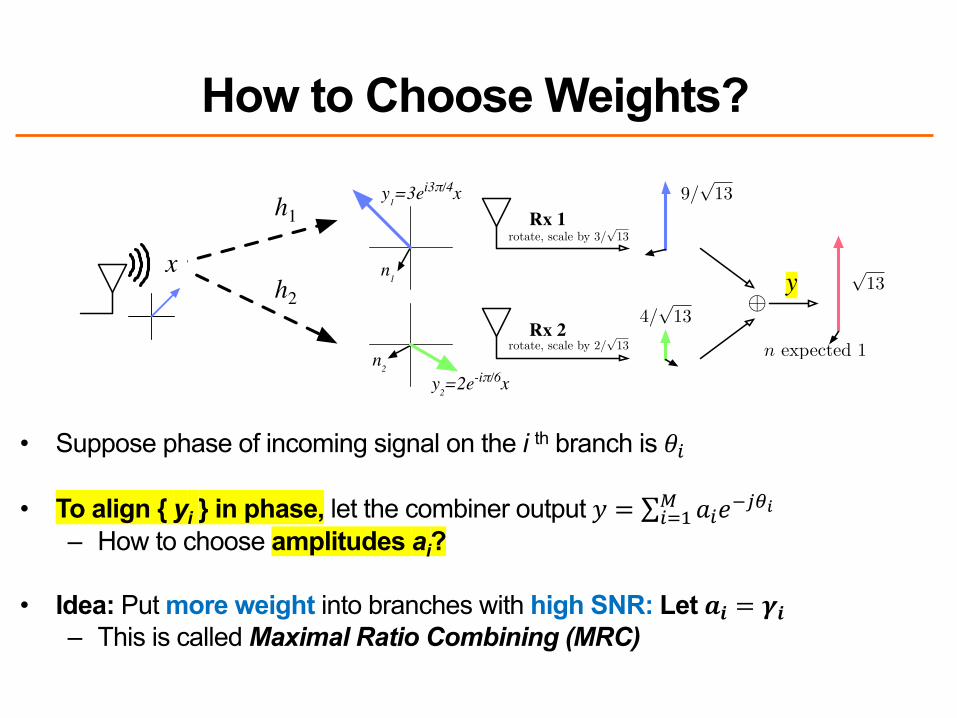
• Suppose phase of incoming signal on the i th branch is !"

• To align { yi } in phase, let the combiner output # = ∑"&'( )"*+,-.– How to choose amplitudes ai?

• Idea: Put more weight into branches with high SNR: Let /0 = 10– This is called Maximal Ratio Combining (MRC)

n2

y2=2e-iπ/6x

rotate, scale by 2/p

13

rotate, scale by 3/p

13

�

9/p

13

4/p

13

p13

x

n expected 1

y1=3ei3π/4x

n1

Figure 3: MRC operation on a sample channel. The channel gains are ~h = h3ei3⇡/4

, 2e�i⇡/6i, with Gaussian

noise ~n = hn1, n2i of expected power 1. The antennas have respective SNRs of 9 and 4. To implement MRC,

the receiver multiplies the received signal ~y = ~hx + ~n by the unit vector ~h⇤/||~h||, where ~h

⇤ denotes the complex

conjugate of ~h. This operation scales each antenna’s signal by its magnitude, and rotates the signals intothe same phase reference before adding them. (For graphical clarity, we depict the common phase vertically,rather than at 0). The resulting sum has magnitude

p13, and expected noise power 1 because the scaling is

normalized. Thus, by coherently combining received signals from di↵erent antennas, the MRC output hasthe expected SNR of 13. In systems with OFDM, MRC is performed separately for each subcarrier.

second node. This is known as a 1x2 system. Real systemsmay have more than two receive antennas, but two will suf-fice for our explanation. With this setup, each receive an-tenna receives a copy of the transmitted signal modified bythe channel between the transmitter and itself. The chan-nel gains hij are complex numbers that represent both theamplitude attenuation over the channel as well as the path-dependent phase shift (see Figure 3 for a graphical example).The receiver measures the channel gains based on trainingfields in the packet preamble. Note that the gains di↵er foreach subcarrier (in frequency-selective fading) as well as foreach antenna. The question now is how to combine the tworeceived signals to make best use of them.

We consider two diversity techniques to show the extremes.The simplest method is to use the antenna with the strongestsignal (hence the largest SNR) to receive the packet and ig-nore the others. We will call this method SEL, for selection

combining. This is essentially what is done by 802.11a/g APswith multiple antennas. It helps with reliability, becauseboth signals are unlikely to be bad, but it wastes perfectlygood received power at the antennas that are not chosen.

The better method is to add the signals from the twoantennas together. However, this cannot be done by simplysuperimposing their signals, or we will have just recreatedthe e↵ects of multi-path fading. Rather, the signals shouldeach be delayed until they are in the same phase; then, thepower in the signals will combine coherently. To do this,the receiver needs a dedicated RF chain for each antenna toprocess the signals. This increases the hardware complexityand power consumption, but yields better performance.

As a twist in the above, the signals are also weighted bytheir SNRs. This gives less weight to a signal that has alarger fraction of noise, so that the e↵ects of the noise are notamplified. The result is maximal-ratio combining, or MRC.MRC is known to be optimal (it maximizes SIMO capacity),and produces an SNR that is the sum of the componentSNRs. Note that in frequency-selective fading, this processis performed di↵erently for each subcarrier according to itsspecific channel gains.

Figure 3 depicts MRC operation graphically for a 1x2channel. In this example, the two channel gains have magni-

-25

-20

-15

-10

-5

0

-20 -10 0 10 20

No

rma

lize

d p

ow

er

(dB

)

Subcarrier index

AC

B and SELAB (MRC)

ABC (MRC)

Figure 4: Frequency-selective fading over testbedlinks: the figure shows, for an example 5.2 GHz link,the received power measured on each subcarrier forindividual antennas and under SEL and MRC diver-sity, normalized to the strongest subcarrier power.

tudes of 3 and 2. With expected noise power 1, these gainscorrespond to SNRs of 9 and 4, given that a signal’s power isthe square of its magnitude. The MRC receiver scales eachantenna’s signal by its magnitude, normalized to the total;delays the signals to a common phase reference; and thenadds them. The result has magnitude

p13, and the normal-

ized weighted sum of noise still has expected power 1. Thecombined signal thus has a resulting sum SNR of 13.

As an example of how MRC and SEL work in 802.11, con-sider Figure 4. This figure shows the wireless signal strengthof each subcarrier using three antennas for a real 802.11n linkin our indoor wireless testbed. The subcarrier strengths aremeasured in decibels normalized to the strongest subcarrierstrength. This figure gives a much more detailed view thanmetrics such as the RSSI (Received Signal Strength Indi-cation) for a link, which gives only the sum of the signalstrength over all subcarriers.

For each antenna labeled A, B, or C, the signal variesover the channel, changing gradually from one subcarrier

Figure 1: A graphical view of the OFDM encoding process for the 18 Mbps rate (QPSK, 3/4) of 802.11a.The data bits (0) are encoded by a rate-1/2 convolutional code (1) and then optionally punctured by droppingcertain bits for higher coding rates (here, 3/4) that send fewer redundant bits (2). The remaining bits are in-terleaved (3) to spread the redundancy across subcarriers and protect against frequency-selective fades. Thesebits are grouped into symbols (4) based on the modulation (QPSK encodes 2 bits per symbol), modulated (5),and finally mapped onto the di↵erent subcarriers to form an OFDM symbol (6).

h11

h12

h11

h12y = x2

Tx Rx

y = xx

1

(a) Receive diversity

h11

h21

h11 h21

Tx Rx

x

x

( + ) xy =

y

(b) Transmit diversity

x1

x2

h11

h12h21

h22

h11x1 h21x2

h12x1 h22x2y2 = +

Tx Rx

y = 1 +

(c) Spatial multiplexing

Figure 2: Using some of the transmit/receive antennas in an example 2x2 system to exploit diversity andmultiplexing gain. xi and yi represent transmitted and received signals. The channel gain hij is a complexnumber indicating a signal’s attenuated amplitude and phase shift over the channel between the ith transmitantenna and the jth receive antenna. The received signals yi will additionally include thermal RF noise.

modulation sending more bits per symbol and being usedwhen there is a higher SNR. There are minor di↵erences be-tween 802.11a/g and 802.11n. In 802.11a/g there are 48 datasubcarriers, 4 pilot tones for control, and 6 unused guardsubcarriers at each edge of the channel. In 802.11n, thereare only 4 guard subcarriers at each edge of the channel, andtwo adjacent 20 MHz channels can be merged into a single40 MHz channel.

The beauty of OFDM is that it divides the channel in away that is both computationally and spectrally e�cient.High aggregate data rates can be achieved, while the en-coding and decoding on di↵erent subcarriers can use sharedhardware components. More relevant to our point here, how-ever, is that OFDM transforms a single large channel intomany relatively independently faded channels. This is be-cause multi-path fading is frequency selective, so the di↵er-ent subcarriers will experience di↵erent fades. Some adja-cent subcarriers may be faded in a similar way, but the fadingfor more distant subcarriers is often uncorrelated. Dividingthe channel also increases the symbol time per channel, sincemany slow symbols will be sent in parallel instead of manyfast symbols in sequence. This adds time diversity becausethe channel is more likely to average out fades over a longerperiod of time.

802.11 makes use of the frequency diversity provided byOFDM by coding across the data carried on the subcarriers.This uses a fraction of them for redundant information thatcan later be used to correct errors that occur when fadingreduces the SNR on some of the subcarriers. First, a con-

volutional code of rate 1/2 adds redundant information. Itis then punctured [3] by removing bits as needed to supportcoding rates of 2/3 and 3/4, plus 5/6 for 802.11n. At a rateof 3/4, for example, a quarter of the data on the subcarriersis redundant. An alternative LDPC (Low-Density Parity-Check) code with slightly better performance can also beused for 802.11n. Figure 1 presents a pictorial overview ofthe OFDM encoding process.

The net e↵ect of OFDM plus coding is to provide consis-tently good 802.11 performance despite significant variabil-ity in the wireless signal due to multi-path fading.

3. SPATIAL DIVERSITYIn this section we look at spatial diversity techniques that

can be applied at the receiver and at the transmitter. Addingmultiple antennas to an 802.11n receiver or transmitter pro-vides a new set of independently faded paths, even if theantennas are separated by only a few centimeters. Thisadds spatial diversity to the system, which can be exploitedto improve resilience to fades. There is also a power gainfrom multiple receive antennas because, everything else be-ing equal, two receive antennas will receive twice the signal.These factors combine to improve performance at a givendistance, and hence increase range.

3.1 Receive Diversity TechniquesConsider the arrangement in Figure 2(a). One transmit

antenna at a node is sending to two receive antennas at a

h1

h2x

Rx 1

Rx 2

y

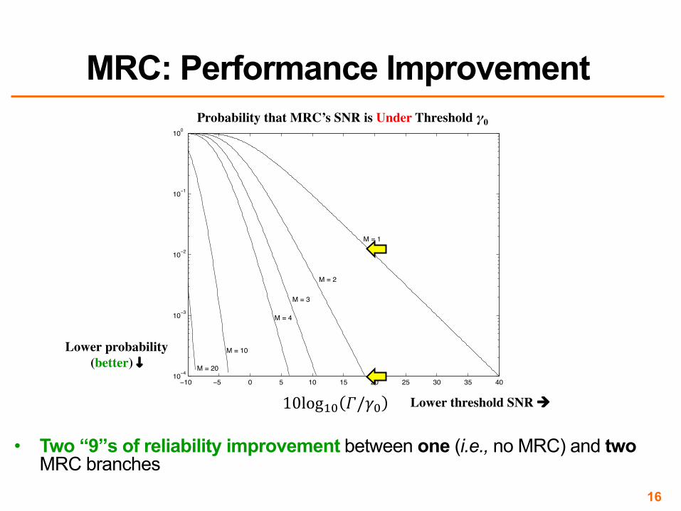
• Two “9”s of reliability improvement between one (i.e., no MRC) and twoMRC branches

16

MRC: Performance Improvement

−10 −5 0 5 10 15 20 25 30 35 4010−4

10−3

10−2

10−1

100

P out

10log10(γ/γ0)

M = 1

M = 2

M = 3

M = 4

M = 10

M = 20

Figure 7.5: Pout for MRC with i.i.d. Rayleigh fading.

Rayleigh fading, where pγΣ(γ) is given by (7.16), it can be shown that [4, Chapter 6.3]

P b =! ∞

0Q("

2γ)pγΣ(γ)dγ =#1 − Γ

2

$M M−1%

m=0

&

M − 1 + mm

'#1 + Γ

2

$m

, (7.18)

where Γ ="

γ/(1 + γ). This equation is plotted in Figure 7.6. Comparing the outage probabilityfor MRC in Figure 7.5 with that of SC in Figure 7.2 or the average probability of error for MRC inFigure 7.6 with that of SC in Figure 7.3 indicates that MRC has significantly better performance thanSC. In Section 7.7 we will use a different analysis based on MGFs to compute average error probabilityunder MRC, which can be applied to any modulation type, any number of diversity branches, and anyfading distribution on the different branches.

7.6 Equal-Gain Combining

MRC requires knowledge of the time-varying SNR on each branch, which can be very difficult to mea-sure. A simpler technique is equal-gain combining, which co-phases the signals on each branch and thencombines them with equal weighting, αi = e−θi . The SNR of the combiner output, assuming equal noisepower N in each branch, is then given by

γΣ =1

NM

&M%

i=1

ri

'2

. (7.19)

212

Probability that MRC’s SNR is Under Threshold γ0

Lower probability (better) ↓

10log'( )/+( Lower threshold SNR à

Selection Diversity, in Frequency

• Antennas A and C experience different fades on different subcarriers

• Selection Combining (“SEL”) improvesbut certain subcarriers still experience fading

• MRC increases power and flattens nulls, leading to fewer bit errors

n2

y2=2e-iπ/6x

rotate, scale by 2/p

13

rotate, scale by 3/p

13

�

9/p

13

4/p

13

p13

x

n expected 1

y1=3ei3π/4x

n1

Figure 3: MRC operation on a sample channel. The channel gains are ~h = h3ei3⇡/4

, 2e�i⇡/6i, with Gaussian

noise ~n = hn1, n2i of expected power 1. The antennas have respective SNRs of 9 and 4. To implement MRC,

the receiver multiplies the received signal ~y = ~hx + ~n by the unit vector ~h⇤/||~h||, where ~h

⇤ denotes the complex

conjugate of ~h. This operation scales each antenna’s signal by its magnitude, and rotates the signals intothe same phase reference before adding them. (For graphical clarity, we depict the common phase vertically,rather than at 0). The resulting sum has magnitude

p13, and expected noise power 1 because the scaling is

normalized. Thus, by coherently combining received signals from di↵erent antennas, the MRC output hasthe expected SNR of 13. In systems with OFDM, MRC is performed separately for each subcarrier.

second node. This is known as a 1x2 system. Real systemsmay have more than two receive antennas, but two will suf-fice for our explanation. With this setup, each receive an-tenna receives a copy of the transmitted signal modified bythe channel between the transmitter and itself. The chan-nel gains hij are complex numbers that represent both theamplitude attenuation over the channel as well as the path-dependent phase shift (see Figure 3 for a graphical example).The receiver measures the channel gains based on trainingfields in the packet preamble. Note that the gains di↵er foreach subcarrier (in frequency-selective fading) as well as foreach antenna. The question now is how to combine the tworeceived signals to make best use of them.

We consider two diversity techniques to show the extremes.The simplest method is to use the antenna with the strongestsignal (hence the largest SNR) to receive the packet and ig-nore the others. We will call this method SEL, for selection

combining. This is essentially what is done by 802.11a/g APswith multiple antennas. It helps with reliability, becauseboth signals are unlikely to be bad, but it wastes perfectlygood received power at the antennas that are not chosen.

The better method is to add the signals from the twoantennas together. However, this cannot be done by simplysuperimposing their signals, or we will have just recreatedthe e↵ects of multi-path fading. Rather, the signals shouldeach be delayed until they are in the same phase; then, thepower in the signals will combine coherently. To do this,the receiver needs a dedicated RF chain for each antenna toprocess the signals. This increases the hardware complexityand power consumption, but yields better performance.

As a twist in the above, the signals are also weighted bytheir SNRs. This gives less weight to a signal that has alarger fraction of noise, so that the e↵ects of the noise are notamplified. The result is maximal-ratio combining, or MRC.MRC is known to be optimal (it maximizes SIMO capacity),and produces an SNR that is the sum of the componentSNRs. Note that in frequency-selective fading, this processis performed di↵erently for each subcarrier according to itsspecific channel gains.

Figure 3 depicts MRC operation graphically for a 1x2channel. In this example, the two channel gains have magni-

-25

-20

-15

-10

-5

0

-20 -10 0 10 20

No

rma

lize

d p

ow

er

(dB

)

Subcarrier index

AC

B and SELAB (MRC)

ABC (MRC)

Figure 4: Frequency-selective fading over testbedlinks: the figure shows, for an example 5.2 GHz link,the received power measured on each subcarrier forindividual antennas and under SEL and MRC diver-sity, normalized to the strongest subcarrier power.

tudes of 3 and 2. With expected noise power 1, these gainscorrespond to SNRs of 9 and 4, given that a signal’s power isthe square of its magnitude. The MRC receiver scales eachantenna’s signal by its magnitude, normalized to the total;delays the signals to a common phase reference; and thenadds them. The result has magnitude

p13, and the normal-

ized weighted sum of noise still has expected power 1. Thecombined signal thus has a resulting sum SNR of 13.

As an example of how MRC and SEL work in 802.11, con-sider Figure 4. This figure shows the wireless signal strengthof each subcarrier using three antennas for a real 802.11n linkin our indoor wireless testbed. The subcarrier strengths aremeasured in decibels normalized to the strongest subcarrierstrength. This figure gives a much more detailed view thanmetrics such as the RSSI (Received Signal Strength Indi-cation) for a link, which gives only the sum of the signalstrength over all subcarriers.

For each antenna labeled A, B, or C, the signal variesover the channel, changing gradually from one subcarrier

• MRC with M branches increases SNR– Increased Shannon capacity

• Sub-linear (logarithmic) capacity increase in M:– !"#$ = &' ( log 1 +. ( /01 bits/second/Hz

MRC’s Capacity Increase

1. Today: Diversity in Space– Receive Diversity– Transmit Diversity

• Channel reciprocity• Transmit beamforming• Introduction to Space-Time Coding: Alamouti’s Scheme

2. Next time: Multiplexing in Space

3. Next time: Interference Alignment

19

Plan

• Forward channel (T to R) is ℎ"# = %& '()*+,/. + %)'()*+0/.

• Switch T and R roles, changing nothing else:– Reverse channel (R to T) is ℎ#" = %& '()*+,/. + %)'()*+0/. = ℎ"#– The reverse radio channel is “reciprocal”

• Practical radio receiver circuitry induces differences between ℎ"#, ℎ#"

20

An Aside: Radio Channels are “Reciprocal”

Receiver RTransmitter T a1,d1,τ1

a2,d2,τ2

• More space, power, processing capability available at the transmitter?– Yes, likely! e.g. Cellular base station, Wi-Fi AP transmitting

downlink traffic to mobile

• But, a (possible) requirement: May need to know the radio channel at the transmitter before the transmission commences– cf. receive diversity: channel from preamble reception

• Then, a tension: Separate transmit antennas for path diversity– Antenna 1, Antenna 2, transmit radio non co-located

• Then, harder to move transmit signals, radio channel measurements i.e. channel state information (CSI) between the three locations

21

Transmit Diversity: Motivation

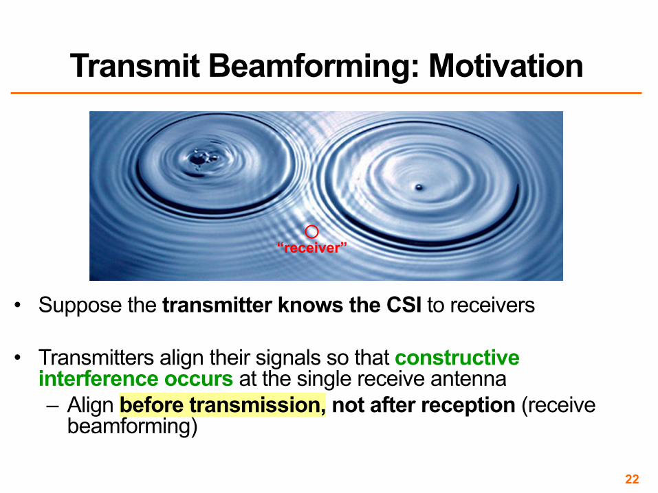
• Suppose the transmitter knows the CSI to receivers

• Transmitters align their signals so that constructive interference occurs at the single receive antenna– Align before transmission, not after reception (receive

beamforming)

22

Transmit Beamforming: Motivation

“receiver”

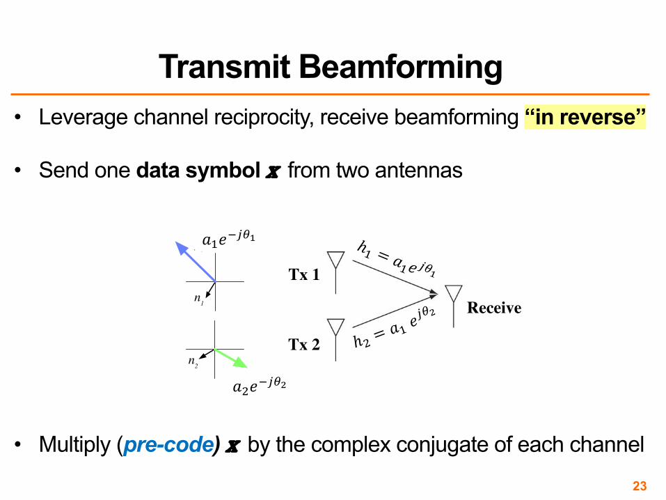
• Leverage channel reciprocity, receive beamforming “in reverse”

• Send one data symbol x from two antennas

23

Transmit Beamforming

n2

y2=2e-iπ/6x

rotate, scale by 2/p

13

rotate, scale by 3/p

13

�

9/p

13

4/p

13

p13

x

n expected 1

y1=3ei3π/4x

n1

Figure 3: MRC operation on a sample channel. The channel gains are ~h = h3ei3⇡/4

, 2e�i⇡/6i, with Gaussian

noise ~n = hn1, n2i of expected power 1. The antennas have respective SNRs of 9 and 4. To implement MRC,

the receiver multiplies the received signal ~y = ~hx + ~n by the unit vector ~h⇤/||~h||, where ~h

⇤ denotes the complex

conjugate of ~h. This operation scales each antenna’s signal by its magnitude, and rotates the signals intothe same phase reference before adding them. (For graphical clarity, we depict the common phase vertically,rather than at 0). The resulting sum has magnitude

p13, and expected noise power 1 because the scaling is

normalized. Thus, by coherently combining received signals from di↵erent antennas, the MRC output hasthe expected SNR of 13. In systems with OFDM, MRC is performed separately for each subcarrier.

second node. This is known as a 1x2 system. Real systemsmay have more than two receive antennas, but two will suf-fice for our explanation. With this setup, each receive an-tenna receives a copy of the transmitted signal modified bythe channel between the transmitter and itself. The chan-nel gains hij are complex numbers that represent both theamplitude attenuation over the channel as well as the path-dependent phase shift (see Figure 3 for a graphical example).The receiver measures the channel gains based on trainingfields in the packet preamble. Note that the gains di↵er foreach subcarrier (in frequency-selective fading) as well as foreach antenna. The question now is how to combine the tworeceived signals to make best use of them.

We consider two diversity techniques to show the extremes.The simplest method is to use the antenna with the strongestsignal (hence the largest SNR) to receive the packet and ig-nore the others. We will call this method SEL, for selection

combining. This is essentially what is done by 802.11a/g APswith multiple antennas. It helps with reliability, becauseboth signals are unlikely to be bad, but it wastes perfectlygood received power at the antennas that are not chosen.

The better method is to add the signals from the twoantennas together. However, this cannot be done by simplysuperimposing their signals, or we will have just recreatedthe e↵ects of multi-path fading. Rather, the signals shouldeach be delayed until they are in the same phase; then, thepower in the signals will combine coherently. To do this,the receiver needs a dedicated RF chain for each antenna toprocess the signals. This increases the hardware complexityand power consumption, but yields better performance.

As a twist in the above, the signals are also weighted bytheir SNRs. This gives less weight to a signal that has alarger fraction of noise, so that the e↵ects of the noise are notamplified. The result is maximal-ratio combining, or MRC.MRC is known to be optimal (it maximizes SIMO capacity),and produces an SNR that is the sum of the componentSNRs. Note that in frequency-selective fading, this processis performed di↵erently for each subcarrier according to itsspecific channel gains.

Figure 3 depicts MRC operation graphically for a 1x2channel. In this example, the two channel gains have magni-

-25

-20

-15

-10

-5

0

-20 -10 0 10 20

No

rma

lize

d p

ow

er

(dB

)

Subcarrier index

AC

B and SELAB (MRC)

ABC (MRC)

Figure 4: Frequency-selective fading over testbedlinks: the figure shows, for an example 5.2 GHz link,the received power measured on each subcarrier forindividual antennas and under SEL and MRC diver-sity, normalized to the strongest subcarrier power.

tudes of 3 and 2. With expected noise power 1, these gainscorrespond to SNRs of 9 and 4, given that a signal’s power isthe square of its magnitude. The MRC receiver scales eachantenna’s signal by its magnitude, normalized to the total;delays the signals to a common phase reference; and thenadds them. The result has magnitude

p13, and the normal-

ized weighted sum of noise still has expected power 1. Thecombined signal thus has a resulting sum SNR of 13.

As an example of how MRC and SEL work in 802.11, con-sider Figure 4. This figure shows the wireless signal strengthof each subcarrier using three antennas for a real 802.11n linkin our indoor wireless testbed. The subcarrier strengths aremeasured in decibels normalized to the strongest subcarrierstrength. This figure gives a much more detailed view thanmetrics such as the RSSI (Received Signal Strength Indi-cation) for a link, which gives only the sum of the signalstrength over all subcarriers.

For each antenna labeled A, B, or C, the signal variesover the channel, changing gradually from one subcarrier

ℎ# = %#& '()

ℎ* = %#&'(+

%#&,'()

%*&,'(+

• Multiply (pre-code) x by the complex conjugate of each channel

Tx 1

Tx 2

Receive

1. Today: Diversity in Space– Receive Diversity– Transmit Diversity

• Channel reciprocity• Transmit beamforming• Introduction to Space-Time Coding: Alamouti’s Scheme

2. Next time: Multiplexing in Space

3. Next time: Interference Alignment

24

Plan

• Suppose transmitters don’t know CSI information to receiver: what to do?

1. Naïve beamforming (just send same signals)– Signals would often cancel out

2. Repetition– Each antenna takes turns transmitting same symbol

• Receiver combines coherently

– Use M symbol times• Increases diversity (“SNR” term in Shannon capacity)• Cuts Shannon rate by 1/M factor

25

Alamouti Scheme: Motivation

• Scope: A two-antenna transmit diversity system (M = 2)

• Sends two symbols, s1 and s2, in two symbol time periods:

Symbol Time Period 1 2Antenna 1: Send !" Send −!$∗Antenna 2: Send !$ Send !"∗

• Then, by superposition the receiver hears:

Symbol Time Period 1 2Receiver hears: ℎ"!" + ℎ$!$ −ℎ"!$∗ + ℎ$!"∗

26

Alamouti Scheme

Symbol Time Period 1 2Receiver hears: y[1] = ℎ'(' + ℎ*(* +[2] = −ℎ'(*∗ + ℎ*('∗

+∗ 2 = ℎ*∗(' − ℎ'∗(*+[1]+∗[2] =

ℎ' ℎ*ℎ*∗ −ℎ'∗

('(*

• Rewrite into two equations in two unknowns (s1 and s2):– (Receiver has CSI information)

('(* ∝ ℎ'∗ ℎ*

ℎ*∗ −ℎ'+[1]+∗[2]

• But, what’s happening in terms of the physical wireless channel?

27

Alamouti Receiver Processing

• Start with the inverted channel matrix:

!"#$ ∝ &"∗ &(

ℎ$∗ −ℎ+,[1],∗[2]

• Consider the computation for s1:– Rotate ,[1] by −1"– Rotate ,∗[2] by 1(– Sum the result

28

Intuition for Alamouti Receiver Processing

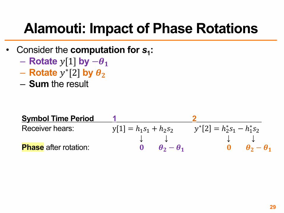
• Consider the computation for s1:– Rotate ![1] by −&'– Rotate !∗[2] by &*– Sum the result

Symbol Time Period 1 2Receiver hears: y[1] = ℎ./. + ℎ1/1 !∗ 2 = ℎ1∗/. − ℎ.∗/1

↓ ↓ ↓ ↓Phase after rotation: 2 &* − &' 2 &* − &'

29

Alamouti: Impact of Phase Rotations

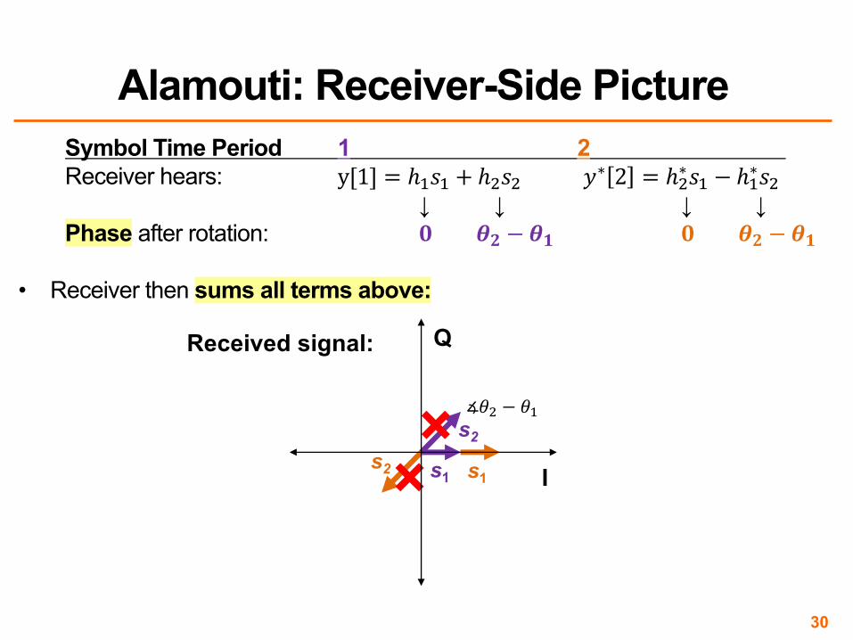
Symbol Time Period 1 2Receiver hears: y[1] = ℎ'(' + ℎ*(* +∗ 2 = ℎ*∗(' − ℎ'∗(*

↓ ↓ ↓ ↓Phase after rotation: / 01 − 02 / 01 − 02

• Receiver then sums all terms above:

30

Alamouti: Receiver-Side Picture

∡4* − 4'

s1

Received signal:

I

Q

s1

s2s2

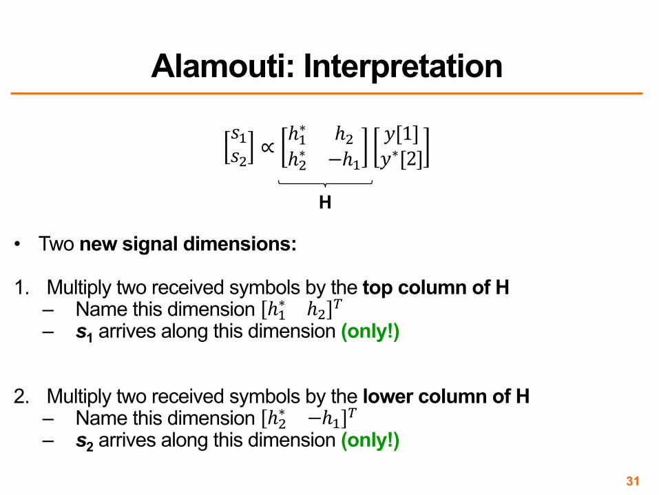
!"!# ∝ ℎ"∗ ℎ#

ℎ#∗ −ℎ"([1](∗[2]

• Two new signal dimensions:

1. Multiply two received symbols by the top column of H– Name this dimension ℎ"∗ ℎ# -– s1 arrives along this dimension (only!)

2. Multiply two received symbols by the lower column of H– Name this dimension ℎ#∗ −ℎ" -– s2 arrives along this dimension (only!)

31

Alamouti: Interpretation

H

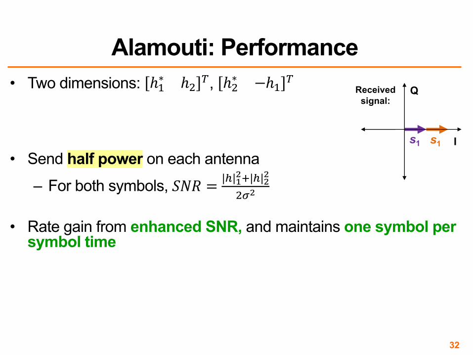
• Two dimensions: ℎ"∗ ℎ$ %, ℎ$∗ −ℎ" %

• Send half power on each antenna

– For both symbols, '() = |,|-./|,|..$0.

• Rate gain from enhanced SNR, and maintains one symbol per symbol time

32

Alamouti: Performance

s1

Receivedsignal:

I

Q

s1

• Leverage path diversity– Decrease probability of “falling into” to deep Rayleigh fade on

a single link

• Defined new “dimensions” of independent communication channels based on space

33

Multi-Antenna Diversity: Summary

Thursday Topic:MIMO II: Spatial Multiplexing

Friday Precept:Exploiting Doppler

34