1

Solution of Linear Systems

2

in matrix form

• AX=B can be transformed into an equivalent system which may be easier to solve.

• Equivalent system has the same solution as the original system.

• Allowable operations during the transformation are:

3

Gaussian Elimination for solving

consists of 2 steps

1. Forward Elimination of unknownsThe goal of Forward Elimination is to transform the coefficient matrix into an Upper Triangular Matrix

2. Back SubstitutionThe goal of Back Substitution is to solve each of the equations using the upper triangular matrix.

[ ][ ] [ ]CXA =

7.00056.18.40

1525

⎥⎥⎥

⎦

⎤

⎢⎢⎢

⎣

⎡−−→

⎥⎥⎥

⎦

⎤

⎢⎢⎢

⎣

⎡

11214418641525

4

Gaussian Elimination

Example 3.16

5

Forward Elimination

Linear EquationsA set of n equations and n unknowns

11313212111 ... bxaxaxaxa nn =++++

22323222121 ... bxaxaxaxa nn =++++

nnnnnnn bxaxaxaxa =++++ ...332211

. .

. .

. .

Forward Elimination

Transform to an Upper Triangular MatrixStep 1: Eliminate x1 in 2nd equation using equation 1 as the pivot equation (pivot row)

)(121

11

aa

Eqn×⎥⎦

⎤⎢⎣

⎡

Which will yield

111

211

11

21212

11

21121 ... b

aaxa

aaxa

aaxa nn =+++

a11:pivot element, row 1:pivot row

6

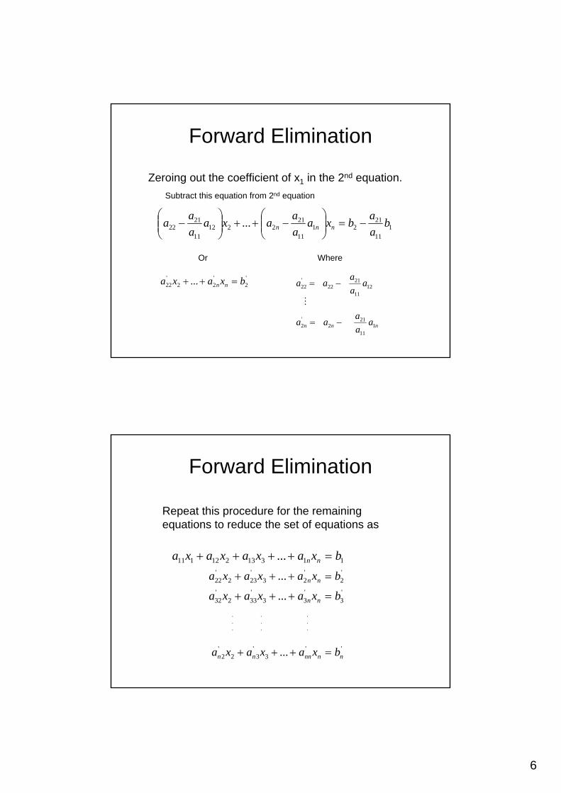
Forward Elimination

Zeroing out the coefficient of x1 in the 2nd equation.Subtract this equation from 2nd equation

111

2121

11

212212

11

2122 ... b

aabxa

aaaxa

aaa nnn −=⎟⎟

⎠

⎞⎜⎜⎝

⎛−++⎟⎟

⎠

⎞⎜⎜⎝

⎛−

'2

'22

'22 ... bxaxa nn =++

nnn aaaaa

aaa

aa

111

212

'2

1211

2122

'22

−=

−=

M

Or Where

Forward Elimination

Repeat this procedure for the remaining equations to reduce the set of equations as

11313212111 ... bxaxaxaxa nn =++++'2

'23

'232

'22 ... bxaxaxa nn =+++

'3

'33

'332

'32 ... bxaxaxa nn =+++

''3

'32

'2 ... nnnnnn bxaxaxa =+++

. . .

. . .

. . .

7

Forward Elimination

Step 2: Eliminate x2 in the 3rd equation.Equivalent to eliminating x1 in the 2nd equation using equation 2 as the pivot equation.

)(23 3222

aa

EqnEqn ×⎥⎦

⎤⎢⎣

⎡−

Forward Elimination

This procedure is repeated for the remaining equations to reduce the set of equations as

11313212111 ... bxaxaxaxa nn =++++'2

'23

'232

'22 ... bxaxaxa nn =+++

"3

"33

"33 ... bxaxa nn =++

""3

"3 ... nnnnn bxaxa =++

. .

. .

. .

8

Forward Elimination

Continue this procedure by using the third equation as the pivotequation and so on.

At the end of (n-1) Forward Elimination steps, the system of equations will look like:

'2

'23

'232

'22 ... bxaxaxa nn =+++

"3

"3

"33 ... bxaxa nn =++

( ) ( )11 −− = nnn

nnn bxa

. .. .. .

11313212111 ... bxaxaxaxa nn =++++

Forward Elimination

At the end of the Forward Elimination steps

⎥⎥⎥⎥⎥⎥

⎦

⎤

⎢⎢⎢⎢⎢⎢

⎣

⎡

=

⎥⎥⎥⎥⎥⎥

⎦

⎤

⎢⎢⎢⎢⎢⎢

⎣

⎡

⎥⎥⎥⎥⎥⎥

⎦

⎤

⎢⎢⎢⎢⎢⎢

⎣

⎡

− )-(nnn

3

2

1

nnn

n

n

n

b

bbb

x

xxx

a

aaaaaaaaa

1

"3

'2

1

)1(

"3

"33

'2

'23

'22

1131211

MMMM

L

L

L

9

Back Substitution

The goal of Back Substitution is to solve each of the equations using the upper triangular matrix.

⎥⎥⎥

⎦

⎤

⎢⎢⎢

⎣

⎡=

⎥⎥⎥

⎦

⎤

⎢⎢⎢

⎣

⎡

⎥⎥⎥

⎦

⎤

⎢⎢⎢

⎣

⎡

3

2

1

3

2

1

33

2322

131211

xxx

00

0bbb

aaaaaa

Example of a system of 3 equations

Back Substitution

Start with the last equation because it has only one unknown

)1(

)1(

−

−

= nnn

nn

n ab

x

Solve the second from last equation (n-1)th

using xn solved for previously.

This solves for xn-1.

10

Back Substitution

Representing Back Substitution for all equations by formula

( ) ( )

( )11

11

−+=

−− ∑−= i

ii

n

ijj

iij

ii

i a

xabx For i=n-1, n-2,….,1

and

)1(

)1(

−

−

= nnn

nn

n ab

x

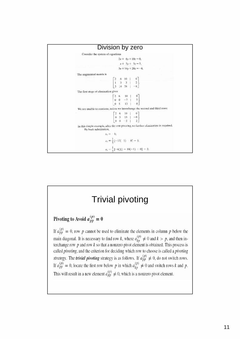
Potential Pitfalls-Division by zero: May occur in the forward elimination steps.

-Round-off error: Prone to round-off errors.

Increase the number of significant digitsDecreases round off error

Does not avoid division by zero

Gaussian Elimination with PivotingAvoids division by zero

Reduces round off error

Improvements

11

Division by zero

Trivial pivoting

12

Round-off error

Pivoting to reduce error

• Partial pivoting• Scaled partial pivoting

13

Partial Pivoting

pka

Gaussian Elimination with partial pivoting applies row switching to normal Gaussian Elimination.

How?At the beginning of the kth step of forward elimination, find the maximum of

nkkkkk aaa .......,,........., ,1+

If the maximum of the values is In the pth row, ,npk ≤≤

then switch rows p and k.

( find max of all elements in the column on or below the main diagonal )

Partial Pivoting

What does it Mean?

Gaussian Elimination with Partial Pivoting ensures that each step of Forward Elimination is performed with the pivoting element |akk| having the largest absolute value.

14

Partial Pivoting: ExampleConsider the system of equations

6x5xx5901.3x3x099.2x3

7x7x10

321

321

21

=+−=++−

=−

In matrix form

⎥⎥⎥

⎦

⎤

⎢⎢⎢

⎣

⎡

−−

5156099.230710

⎥⎥⎥

⎦

⎤

⎢⎢⎢

⎣

⎡

3

2

1

xxx

⎥⎥⎥

⎦

⎤

⎢⎢⎢

⎣

⎡

6901.37

=

Solve using Gaussian Elimination with Partial Pivoting using five significant digits with chopping

Partial Pivoting: Example

Forward Elimination: Step 1Examining the values of the first column

|10|, |-3|, and |5| or 10, 3, and 5

The largest absolute value is 10, which means, to follow the rules of Partial Pivoting, we switch row1 with row1.

⎥⎥⎥

⎦

⎤

⎢⎢⎢

⎣

⎡=

⎥⎥⎥

⎦

⎤

⎢⎢⎢

⎣

⎡

⎥⎥⎥

⎦

⎤

⎢⎢⎢

⎣

⎡

−−

6901.37

5156099.230710

3

2

1

xxx

⎥⎥⎥

⎦

⎤

⎢⎢⎢

⎣

⎡=

⎥⎥⎥

⎦

⎤

⎢⎢⎢

⎣

⎡

⎥⎥⎥

⎦

⎤

⎢⎢⎢

⎣

⎡−−

5.2001.67

55.206001.000710

3

2

1

xxx

⇒Performing Forward Elimination

15

Partial Pivoting: Example

Forward Elimination: Step 2Examining the values of the first column

|-0.001| and |2.5| or 0.0001 and 2.5

The largest absolute value is 2.5, so row 2 is switched with row 3

⎥⎥⎥

⎦

⎤

⎢⎢⎢

⎣

⎡=

⎥⎥⎥

⎦

⎤

⎢⎢⎢

⎣

⎡

⎥⎥⎥

⎦

⎤

⎢⎢⎢

⎣

⎡−−

5.2001.67

55.206001.000710

3

2

1

xxx

⇒⎥⎥⎥

⎦

⎤

⎢⎢⎢

⎣

⎡=

⎥⎥⎥

⎦

⎤

⎢⎢⎢

⎣

⎡

⎥⎥⎥

⎦

⎤

⎢⎢⎢

⎣

⎡

−

−

001.65.2

7

6001.0055.200710

3

2

1

xxx

Performing the row swap

Partial Pivoting: Example

Forward Elimination: Step 2

Performing the Forward Elimination results in:

⎥⎥⎥

⎦

⎤

⎢⎢⎢

⎣

⎡=

⎥⎥⎥

⎦

⎤

⎢⎢⎢

⎣

⎡

⎥⎥⎥

⎦

⎤

⎢⎢⎢

⎣

⎡ −

002.65.2

7

002.60055.200710

3

2

1

xxx

16

Partial Pivoting: Example

Back SubstitutionSolving the equations through back substitution

1002.6002.6

3 ==x

15.255.2 2

2 =−

=x

x

010

077 321 =

−+=

xxx

⎥⎥⎥

⎦

⎤

⎢⎢⎢

⎣

⎡=

⎥⎥⎥

⎦

⎤

⎢⎢⎢

⎣

⎡

⎥⎥⎥

⎦

⎤

⎢⎢⎢

⎣

⎡ −

002.65.2

7

002.60055.200710

3

2

1

xxx

Scaled partial pivoting

17

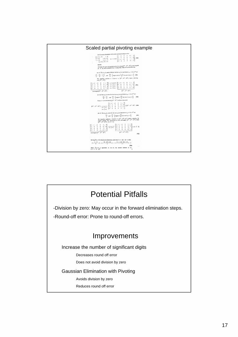
Scaled partial pivoting example

Potential Pitfalls-Division by zero: May occur in the forward elimination steps.

-Round-off error: Prone to round-off errors.

Increase the number of significant digitsDecreases round off error

Does not avoid division by zero

Gaussian Elimination with PivotingAvoids division by zero

Reduces round off error

Improvements

18

LU Decomposition(Triangular Factorization)

LU Decomposition

[ ]L

[ ]A

[ ] [ ][ ]ULA =

[ ]U

A non-singular matrix has a traingular factorization if it can be expressed as

where

= lower triangular martix

= upper triangular martix

19

LU DecompositionMethod: [A] Decompose to [L] and [U]

[ ] [ ][ ]⎥⎥⎥

⎦

⎤

⎢⎢⎢

⎣

⎡

⎥⎥⎥

⎦

⎤

⎢⎢⎢

⎣

⎡==

33

2322

131211

3231

21

000

101001

uuuuuu

ULAll

l

[U] is the same as the coefficient matrix at the end of the forward elimination step.

[L] is obtained using the multipliers that were used in the forward elimination process

Example

20

LU Decomposition

Given

Decompose into and [ ]U[ ]L

Then solve for

And then solve for

[ ][ ] [ ]C=Z L [ ]Z

[ ][ ] [ ]ZU =X [ ]X

[ ][ ] [ ]CXA =

[ ]A [ ][ ][ ] [ ]CXUL =⇒

Define [ ] [ ][ ]XUZ =

LU DecompositionExample: Solving simultaneous linear equations using LU Decomposition

Solve the following set of linear equations using LU Decomposition ⎥

⎥⎥

⎦

⎤

⎢⎢⎢

⎣

⎡=

⎥⎥⎥

⎦

⎤

⎢⎢⎢

⎣

⎡

⎥⎥⎥

⎦

⎤

⎢⎢⎢

⎣

⎡

2.2792.1778.106

aaa

11214418641525

3

2

1

Using the procedure for finding the [L] and [U] matrices

[ ] [ ][ ]⎥⎥⎥

⎦

⎤

⎢⎢⎢

⎣

⎡−−

⎥⎥⎥

⎦

⎤

⎢⎢⎢

⎣

⎡==

7.00056.18.40

1525

15.376.50156.2001

ULA

21

LU Decomposition

[ ]⎥⎥⎥

⎦

⎤

⎢⎢⎢

⎣

⎡−=

⎥⎥⎥

⎦

⎤

⎢⎢⎢

⎣

⎡=

735.021.968.106

3

2

1

zzz

Z

Example: Solving simultaneous linear equations using LU Decomposition

Set

Solve for

[ ][ ] [ ]CZL =

⎥⎥⎥

⎦

⎤

⎢⎢⎢

⎣

⎡=

⎥⎥⎥

⎦

⎤

⎢⎢⎢

⎣

⎡

⎥⎥⎥

⎦

⎤

⎢⎢⎢

⎣

⎡

2.2792.1778.106

15.376.50156.2001

3

2

1

zzz

[ ]Z

LU Decomposition

[ ][ ] [ ]ZXU =

[ ]X

Example: Solving simultaneous linear equations using LU Decomposition

Set

Solve for

⎥⎥⎥

⎦

⎤

⎢⎢⎢

⎣

⎡=

⎥⎥⎥

⎦

⎤

⎢⎢⎢

⎣

⎡

⎥⎥⎥

⎦

⎤

⎢⎢⎢

⎣

⎡−−

0.73596.21-

106.8

7.00056.18.40

1525

3

2

1

aaa

⎥⎥⎥

⎦

⎤

⎢⎢⎢

⎣

⎡=

⎥⎥⎥

⎦

⎤

⎢⎢⎢

⎣

⎡

050.170.19

2900.0

3

2

1

aaa

22

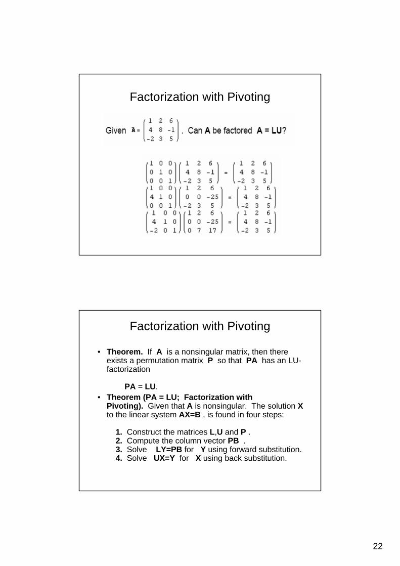
Factorization with Pivoting

Factorization with Pivoting

• Theorem. If A is a nonsingular matrix, then there exists a permutation matrix P so that PA has an LU-factorization

PA = LU.• Theorem (PA = LU; Factorization with

Pivoting). Given that A is nonsingular. The solution Xto the linear system AX=B , is found in four steps:

1. Construct the matrices L,U and P .2. Compute the column vector PB .3. Solve LY=PB for Y using forward substitution.4. Solve UX=Y for X using back substitution.

23

[ ]⎥⎥⎥

⎦

⎤

⎢⎢⎢

⎣

⎡−=

104012001

L

[ ][ ] [ ]CZL =

Is LU Decomposition better or faster than Gauss Elimination?

Let’s look at computational time.

n = number of equations

To decompose [A], time is proportional to

To solve and

time proportional to

3

3n

[ ][ ] [ ]CXU =

2

2n

24

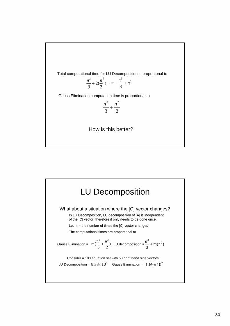
Total computational time for LU Decomposition is proportional to

23

3nn

+)2

(23

23 nn+ or

Gauss Elimination computation time is proportional to

23

23 nn+

How is this better?

LU Decomposition

)2n

3n(m

23

+ )n(m3n 2

3

+

51033.8 ×

What about a situation where the [C] vector changes?In LU Decomposition, LU decomposition of [A] is independent of the [C] vector, therefore it only needs to be done once.

Let m = the number of times the [C] vector changes

The computational times are proportional to

Gauss Elimination = LU decomposition =

Consider a 100 equation set with 50 right hand side vectors

LU Decomposition = Gauss Elimination = 71069.1 ×

25

Jacobi and Gauss-Seidel Method

Simultaneous Linear Equations:Iterative Methods

26

-Algebraically solve each linear equation for xi

-Assume an initial guess

-Solve for each xi and repeat

-Check if error is within a pre-specified tolerance.

Jacobi Gauss-Seidel

27

Algorithm

A set of n equations and n unknowns:

11313212111 ... bxaxaxaxa nn =++++

2323222121 ... bxaxaxaxa n2n =++++

nnnnnnn bxaxaxaxa =++++ ...332211

. .

. .

. .

If: the diagonal elements are non-zero

Rewrite each equation solving for the corresponding unknown

ex:First equation, solve for x1

Second equation, solve for x2

Algorithm

Rewriting each equation

11

131321211 a

xaxaxacx nn−−−=

KK

nn

nnnnnnn

nn

nnnnnnnnnn

nn

axaxaxac

x

axaxaxaxac

x

axaxaxacx

11,2211

1,1

,122,122,111,111

22

232312122

−−

−−

−−−−−−−−

−−−−=

−−−−=

−−−=

KK

KK

MMM

KK

From Equation 1

From equation 2

From equation n-1

From equation n

28

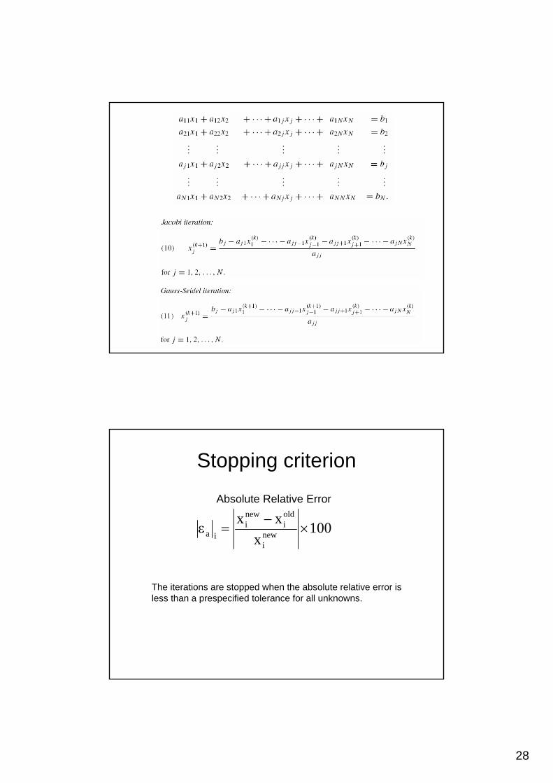
Stopping criterion

Absolute Relative Error

100x

xxnewi

oldi

newi

ia ×−

=ε

The iterations are stopped when the absolute relative error is less than a prespecified tolerance for all unknowns.

29

Given the system of equations1 5x -3x 12x 321 =+

28 3x 5x x 321 =++76 13x 7x 3x 321 =++ ⎥

⎥⎥

⎦

⎤

⎢⎢⎢

⎣

⎡=

⎥⎥⎥

⎦

⎤

⎢⎢⎢

⎣

⎡

101

3

2

1

xxx

With an initial guess of

⎥⎥⎥

⎦

⎤

⎢⎢⎢

⎣

⎡=

⎥⎥⎥

⎦

⎤

⎢⎢⎢

⎣

⎡

⎥⎥⎥

⎦

⎤

⎢⎢⎢

⎣

⎡ −

76281

13733515312

3

2

1

aaa

Rewriting each equation

12531 32

1

xxx +−=

5328 31

2

xxx −−=

137376 21

3

xxx −−=

( ) ( ) 50000.012

150311 =

+−=x

( ) ( ) 9000.45

135.0282 =

−−=x

( ) ( ) 0923.313

9000.4750000.03763 =

−−=x

The absolute relative error

%662.6710050000.0

0000.150000.01a =×

−=∈

%00.1001009000.4

09000.42a =×

−=∈

%662.671000923.3

0000.10923.33a =×

−=∈

The maximum absolute relative error after the first iteration is 100%

After Iteration #1

⎥⎥⎥

⎦

⎤

⎢⎢⎢

⎣

⎡=

⎥⎥⎥

⎦

⎤

⎢⎢⎢

⎣

⎡

0923.39000.45000.0

3

2

1

xxx

⎥⎥⎥

⎦

⎤

⎢⎢⎢

⎣

⎡=

⎥⎥⎥

⎦

⎤

⎢⎢⎢

⎣

⎡

101

3

2

1

xxx

Initial guess

30

Repeating more iterations, the following values are obtained

1aε 2aε 3aε

67.66218.8764.0042

0.657980.074990.00000

3.09233.81183.97083.99714.00014.0001

100.0031.88717.4094.5012

0.822400.11000

4.9003.71533.16443.02813.00343.0001

67.662240.6280.2321.5474.5394

0.74260

0.500000.146790.742750.946750.991770.99919

123456

a3a2a1Iteration

⎥⎥⎥

⎦

⎤

⎢⎢⎢

⎣

⎡=

⎥⎥⎥

⎦

⎤

⎢⎢⎢

⎣

⎡

431

3

2

1

xxx

⎥⎥⎥

⎦

⎤

⎢⎢⎢

⎣

⎡=

⎥⎥⎥

⎦

⎤

⎢⎢⎢

⎣

⎡

0001.40001.3

99919.0

3

2

1

xxx

The solution obtained

the exact solution

31

What went wrong?Even though done correctly, the answer is not converging to the correct answer

This example illustrates a pitfall of Jacobi/ Gauss-Siedel method: not all systems of equations will converge.

Is there a fix?

Diagonally dominant: [A] in [A] [X] = [C] is diagonally dominant if:

∑≠=

>n

jj

ijaai

ii1

The coefficient on the diagonal must be greater than the sum of the other coefficients in that row.