Mechanism and Machine Theory 86 (2015) 1–14

Contents lists available at ScienceDirect

Mechanism and Machine Theory

j ourna l homepage: www.e lsev ie r .com/ locate /mechmt

Speed losses in V-ribbed belt drives

Berna Balta a,b, Fazil O. Sonmez c,⁎, Abdulkadir Cengiz d

a Department of Mechanical Engineering, Kocaeli University, Kocaeli, Umuttepe, 41380, Turkiyeb Ford Otosan, Product Development Department, Kocaeli, Gebze 41470, Turkiyec Department of Mechanical Engineering, Bogazici University, Istanbul, Bebek, 34342, Turkiyed Mechanical Education Department, Kocaeli University, Kocaeli, Umuttepe, 41380, Turkiye

a r t i c l e i n f o

⁎ Corresponding author. Tel.: +90 212 359 7196.E-mail addresses: bguner@ford.com (B. Balta), sonm

http://dx.doi.org/10.1016/j.mechmachtheory.2014.11.010094-114X/© 2014 Elsevier Ltd. All rights reserved.

a b s t r a c t

Article history:Received 11 December 2013Received in revised form 10 November 2014Accepted 24 November 2014Available online xxxx

One of the concerns in belt drive transmissions is the relative sliding (slip) of the belt with respectto the pulley, which results in speed loss, i.e. decrease in the angular velocity of the driven pulley.In this study, the slip behavior of a V-ribbed belt drivewith two equal-sized pulleys is investigatedby utilizing several experimental methodologies. The individual effects of belt-drive parameterson speed loss are determined using one-factor-at-a-time (OFAT) test method. The relationbetween the belt-drive parameters and the speed loss is found using response surface method(RSM). Afterwards, the optimum operating conditions are determined via a design optimizationprocedure. In order to validate the response surface curve, experiments are conducted witharbitrary operating conditions and themeasured and predicted values of speed loss are compared.The predictions of the response surface model are also found to be in good agreement with theempirical results presented in the literature. Furthermore, the predicted model looks reasonablyaccurate based on the analysis of variance (ANOVA) and the residual analysis. Using the responsecurve, onemay estimate the degree of speed loss for similar belt-drives with operating conditionswithin the range considered in the present study.

© 2014 Elsevier Ltd. All rights reserved.

Keywords:V-ribbed belt drivesSlipOFATRSMDesign optimizationANOVA

1. Introduction

Belt drives are power transmission systems commonly used in the industry [1]. There are different types of belts like flat belts,V-belts, and V-ribbed belts. Flat belts offer flexibility, while V-belts offer high power transmission capacity. V-ribbed belts, on theother hand, combine these two properties. They are made of a layer of reinforcing cords as tension-carrying members, a protectivecushion of rubber that envelopes the cords, a rubber backing, and ribs made of short-fiber-reinforced rubber as shown in Fig. 1.

In comparison to the traditional V-belts, V-ribbed belts have numerous advantages including accommodation to smaller pulleyssizes and belt lengths, backside operation, and relatively longer service life. The ribs on V-ribbed belts guide the belt and make itmore stable in comparison to the traditional flat-belts; they also provide increased power transmission capacity by increasing thefriction surface and normal pressure.

High efficiency and high performance of V-ribbed belt drives can only be achieved if proper values are chosen for the designparameters. This requires fundamental understanding of the operational characteristics unique to this class of belts and belt drivesystems. High efficiency can be achieved by decreasing power losses. In belt drives, power losses occur due to a combination ofspeed losses and torque losses [1]. Speed losses result from sliding of the belt relative to the pulley, which leads to a decrease inthe angular velocity of the driven pulley, and thus in the transmitted power. With a proper design of belt drives, power losses can

ezfa@boun.edu.tr (F.O. Sonmez), akcengiz@kocaeli.edu.tr (A. Cengiz).

6

Fig. 1. A scheme for V-ribbed belts.

2 B. Balta et al. / Mechanism and Machine Theory 86 (2015) 1–14

be decreased and, thus, their efficiency can be increased; but this requires fundamental understanding of the effects of the dominantfactors on power loss.

Some researchers theoretically examined the slip behavior in belt drives. In 1874, Reynolds showed that torque transmissionsbetween pulleys involved speed losses due to belt's elastic creep [2]. Gerbert [3] explained the mechanism of slipping by dividingthe arc of contact between belt and pulley into sticking (non-slipping) and slipping regions. The belt was treated as a string andthe mechanism of elastic creep of the belt along the pulley was shown to yield a slip arc at the exit region of the pulley, where theentire transition from the high to low tension occurred. In the remaining contact region, commonly referred to as the stick (non-slip)arc, the belt was shown to stick to the pulley without slipping with no change in tension [4]. Although the classical creep theoryexplains how belt slip occurs to a reasonable extent, speed losses encountered in practice are larger than predicted by extensionalcreep, particularly for thickflat-belts, V-belts, andV-ribbed belts. Firbank [5] proposed a theorywhere shear strain in the belt envelopewas assumed to be the determining factor on the drive behavior. The difference between the two theories is that the creep theoryassumes that belt behavior is governed by the elastic extension and contraction of the belt as opposed to the shear theory. However,both of the assumptions are too strict to explain the slip behavior and the slip regions along the contact region between the belt andthe pulley. Firbank claimed that slip occurred only at the exits of the driver and driven pulleys. The remaining region over the entirearcwas taken as the real arc of contact as defined byGerbert [6]. Gerbert [7] proposed an analysis that considered bothflexural rigidityand compressibility of the belt and assumed that belt speed differences in the entry and exit regionswere observed due to the changein the radius of the curvature of the belt, whichmeant that belt extensibilitywas not the only factor to explain the slip behavior. Sorgeetal. [8] defined the arc of contact as the power transmitting part of the belt and claimed that there was almost no tension variation inthe contact region.

Previous experimental studies on power loss behavior of belt drives usually considered V-belt drives and continuously variabletransmission (CVT) belt drives. Researchers basically used belt drive test setups with two equal-sized-pulleys. Peeken and Fischer[9] developed a V-belt drive test setup to determine the efficiency up to 200 Nm torque and 6000 rpm speed with a fixed shaftdistance. The belt pre-tension was provided by a pivoted rocking arm. They obtained braking torque vs. slip relation for a singlecombination of belt tension, belt length, and pulley diameter.

Childs andCowburn [10] experimentally investigated the effects ofmismatchbetween thewedge angles of pulley grooves and beltribs on the power loss behavior of V-belt drives. During the tests, they kept the other parameters constant. They [11] also studied theeffects of small pulleys on the power loss both theoretically and experimentally. Using pulleyswith diameters ranging from42mmupto 102mm, they examined the effect of braking torque on power loss. In the experiments, the same belt length and belt material wereused.

Lubarda [12] analytically formulated the variation in the belt force over the arc of contact offlat andV-belts before gross slip occurs.He separated the arc of contact into active and non-active regions, similar to the approach of Gerbert [3] and Johnson [4].

A number of studieswere conducted to investigate CVT type belt drives used inmotorcycles with the help of two-pulley-belt drivetest rigs. Ferrando et al. [13] developed a test setup to determine the effects of the drive parameters on the axial force. A velocitycontroller was used tomaintain its speed. Bymeans of electric motors, the driver pulley was actuated and braking torquewas appliedto the driven pulley. The belt tension, the input torque, and the total axial force in the belt were measured. With a similar setup,Amijma et al. [14] studied the effects of acceleration or deceleration on the power transmission behavior of a CVT belt drive bymeasuring the axial force via a load cell at a constant speed (2430 rpm) and a constant braking torque. Chen et al. [15] focused onthe efficiency of a rubber V-belt CVT drive. In the test setup, input and output torques were measured by torque transducers andspeed was measured by optical encoders. Additionally, they installed laser displacement sensors in order to detect the changes inthe pitch radii of CVT pulleys and determined the speed and torque losses under different operating conditions. Akehurst et al.[16–18] investigated the power transmission efficiency of a metal V-belt CVT drive. The belt was constructed from several hundredsegments held together by steel band sets. They formulated the torque loss and belt-slip losses and correlated them with theexperimental results. Bertini et al. [19] studied the power losses in a rubber V-belt type CVT, both experimentally and analytically.They grouped the power loss contributors as hysteresis losses and frictional losses arising at the entrance and exit regions of thepulleys due to engagement/disengagement of the belt. They validated their model through a test bench, which was capable ofmeasuring the transmitted torques, axial trusts on the pulleys, pulley speeds, and belt tension. However, they did not use differentbelts and pulley diameters to evaluate their effects. Mantriota [20–22] performed extensive experiments to study the efficiency ofpower-split CVT (PS-CVT). PS-CVT was obtained by joining a V-belt CVT, a planetary gear train, and a timing belt. Input and outputangular speeds and torques weremeasured bymeans of torque-tachometers integrated to the driving and driven shafts. A regulation

3B. Balta et al. / Mechanism and Machine Theory 86 (2015) 1–14

valve controlled pneumatic disk brake was used to apply output torque [20,21,23]. The efficiency of the PS-CVT systemwas shown tobe notably higher than simple CVT systems [20–22]. A detailed experimental investigation concerning the dynamics of a metalpushing V-belt CVT was conducted by Carbone et al. [24]. They compared the theoretical predictions of Carbone–Mangialardi–Mantriota (CMM)model [25]with the experimental results. They equipped their test rig with sensors tomeasure pressure, rotationalspeed, and pulley-sheave position [24]. In another study, Zhu et al. [26] experimentally measured power losses in a rubber V-belt CVTfor a low-power vehicle like scooters and snowmobiles.

The previous studies considered only flat belt, V-belt, and V-belt CVT drives before V-ribbed belt driveswere introduced in the lastdecades. For this reason, the published papers on V-ribbed belt drives are relatively few [27–36]. Dalgarno et al. [27] developed aV-ribbed-belt-drive test setup with two-pulleys to investigate gross slip-born audible noise. A motor and a generator were installedto provide driver and driven pulley torque loads. The input torque was monitored using an in-line torque transducer. An idlertensioner was used to provide and maintain the belt pre-tension. Also, encoders and a tension transducer were used to measurethe speed and belt tension, respectively. They tested three different types of belts with the same geometrical profile. The noise levelsof these belts were compared at different operating conditions.

Yu et al. [28] developed a two-pulley V-ribbed belt drive system running at 1000 rpm. They applied different levels of brakingtorque and measured the radial position of the belt in the pulley grooves by placing laser displacement sensors over the arc of thedriver and driven pulleys. Yu [29] investigated the parameters affecting mechanical performance of a two-pulley belt drive systemby using four different belts: a new cut belt, a used cut belt, molded belt, and anti-wear belt. Yu et al. [30] also investigated wearingpatterns of V-ribbed belts.

Misalignment is another important issue in belt-drive systems. Xu et al. [31] used a simple static two-pulley test setup for theassessment of lateral forces in misaligned pulleys driving a V-ribbed belt. A dead weight was hanged to one of the pulleys to induceinitial tension and the results obtained under static conditions were correlated with FEA results.

In another V-ribbed belt drive study,Manin et al. [32] investigated the effects of different types of front-end accessory drive (FEAD)tensioners on the belt span vibration and pulley-belt slip. They constructed a four-pulley-belt drive system, including a driver pulleyactuated by an electric motor, a driven pulley, and two idler pulleys; one of which was a tensioner. The speeds of the driver, driven,and tensioner pulleys were measured via encoders, and a laser sensor was also installed to detect belt flapping. Belt pre-tension wasmeasured by a piezo-electric sensor. Driving and driven torques weremeasured via strain gages. They obtained the relation betweenthe slip and the braking torque for three different tensioner types (idler, hydraulic, and dry friction) and two different low speedlevels, 280 and 840 rpm, while keeping the other parameters constant. They also measured the belt slip for two different levels ofbelt tension using one type of belt tensioner.

Cepon et al. [33] studied the effects of contact parameters, i.e. the friction coefficient, normal contact force, and tangential beltvelocity. They measured the belt-pulley contact stiffness and the friction coefficient on two different specific test setups. They alsoconstructed a two-pulley V-ribbed belt drive test setup, where the angular speeds of the driver and driven pulleys were measuredusing two optical encoders. The driving and braking torques were measured by torque transducers. A hydraulic pump was used toapply braking torque to the belt drive system. Their studywas limited to a single combination of belt type, belt length, and pulley size.

Cepon et al. [34], measured the longitudinal stiffness, transverse stiffness, and bending stiffness of V-ribbed belts on a test rig withtwo equal-sized pulleys. In another test rig, they measured the first three natural frequencies of the V-ribbed belt via displacementsensors. They did not study power losses. In the same test rig, Cepon and Boltezar [35] measured the speed losses and longitudinalvibrations of the belt at its tight and slack sides using two displacement sensors. They concluded that because analytical formulationsdepended on the creep theory and neglected the radial and tangential deformations of the belt, analytical results were obtained to befar below the experimental ones.

Pietra and Timpone [36] built up a test rig with two-equal-sized pulleys in order to measure the tension ratio between the tightand slack sides of the belt. They used a dead weight to tension the belt drive and mounted strain gages on the outer surfaces of thebelt to measure the belt tension. They compared their measurements with theoretical results. By using a high speed camera, theyalso measured the slip of a thick V-belt.

In order tominimize slip, Kumar and Sooryaprakash [37] developed a closed loop controlled belt tensioner. The slack and tight sidetensions were measured by means of displacement sensors. The belt tension was maintained at a predetermined value by thetensioner controller, which adjusted the belt tension based on the sensor signals.

Analytical formulations of slip and torque loss were presented previously for flat and V-belt drives: Gerbert [38] analyzed slip andtorque loss in V-belt drives considering the radial compliance and flexural rigidity. Gerbert [3] then derived another analytical formulafor the speed loss of thick flat belts. He accounted for shear deflection, radial compliance, and seating/unseating behavior. Later on,Gerbert [7] extended the analytical slip formulation with a unified approach for flat and V-belts based on the creep theory. Belofsky[39] presented a new formulation for the tension ratio of the tight and slack sides by considering the belt elasticity, flexural rigidity,and variation of friction force along the contact arc. Childs and Cowburn [11] proposed a new formulation for the speed loss andtorque loss behaviors of V-belt drives. They accounted for belt bending stiffness, radial compliance, pulley diameter, and beltpre-tension.

Several studies conducted finite element analyses of flat and V-ribbed belts. Chen and Shieh [40] obtained the speed loss in a flatbelt transmission system by developing a 3D finite element model. Yu et al. [41] constructed a 3D finite element model in order tocalculate the radial positioning of a V-ribbed belt into the pulley grooves.

There are several studies [3–11,38,40] on the slip behavior of flat and V-belt drives. Few studies [27–29,32,34,35] exist on the slipbehavior of V-ribbed belt drives. In those studies, a limited number of belt drive parameters were considered. The effect of belt lengthhas not been studied.

4 B. Balta et al. / Mechanism and Machine Theory 86 (2015) 1–14

In the present study, the effects of the belt-drive parameters on the speed loss behavior of V-ribbed belt drives are experimentallyinvestigated. For this purpose, a test setup is constructed with two equal-sized pulleys to measure the speed losses in a V-ribbed beltdrive system. In comparison to the previous studies, a much larger number of parameters and their interactions are taken intoconsideration; they include belt tension, driver pulley speed, braking torque, belt length, pulley diameter, and belt material. Theeffects of the belt length on the speed loss of V-ribbed belt drives are investigated for the first time. After building the setup, ameasurement system analysis (MSA) is conducted in order to ensure the precision and repeatability of the measured data. Then,the effects of the individual parameters are determined using one-factor-at-a-time (OFAT) testing methodology. Furthermore,using response surface methodology (RSM), the relation between the input parameters and the speed loss is obtained. Finally,optimum operating conditions are determined for minimum speed loss via an optimization procedure.

2. Experimental study

2.1. Experimental setup and instrumentation

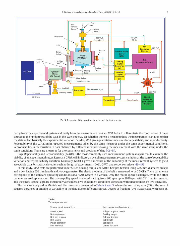
In this study, the setup shown in Fig. 2 and schematically depicted in Fig. 3 is built to investigate the effects of various parameterson the speed loss behavior of V-ribbed belt drives. J-type V-ribbed beltswith four ribs are used to transmit power between the pulleys.The belt drive is actuated by an electric motor having a maximum power output of 3 kW. A frequency inverter is used to control theangular velocity of the driver pulley. Braking torque is applied to the driven pulley by means of a hydraulic pump, which serves as adynamometer. It can be run at different steady state operating conditions by adjusting a valve; in this way, different levels of brakingtorque can be provided. The maximum braking torque capacity is 10 N.m. The controllable input parameters and the measuredparameters are given in Table 1.

In order to be able tomodify the belt tension and accommodate different pulley diameters and belt lengths, themotor is placed ona sliding base. Pre-tension is induced in the belt by means of a spring mechanism, which can apply different levels of force to thesliding base. The total axial force in the belt is measured by a load cell. The dynamometer is mounted on ball bearing housing. Themagnitudes of the reaction forces causing torque are measured by the load cell mounted on the housing. In this study, neglectingthe frictional torques, the torque calculated using the measured values of force at the housing is assumed to be equal to the brakingtorque directly applied by the dynamometer. The angular speeds of the driver and driven pulleys are measured with two opticalencoders. Additionally, a photoelectric switch is installed to count the belt rotation. A linear variable differential transformer(LVDT) sensor is placed next to the driver pulley to detect the radial displacement of the belt into the pulley grooves under tension.In order to measure the central distance between the pulleys, a dial gage is placed to the sliding base on which the motor is mounted.The datameasured by the encoders, photoelectric switch, load cells, and LVDT are processed in themicroprocessors to be converted todigital data; then they are transferred to the computer using a data acquisition software, LabVIEWTM.

2.2. Measurement system analysis (MSA)

MSA is performed at the beginning of an experimental study to ensure that the information collected is a true representation ofwhat is occurring in the experiment. Experimental data collected under the same conditions usually show variation, which arises

Motor

LVDT

SpeedSensor

Load Cell (Spring Force)

Driver Pulley

Driven Pulley

Encoder

Pump

Load Cell for motor

Fig. 2. The experimental setup.

Oil Return

Oil Supply

Oil Tank HydraulicBrake

(Oil Pump)

Driver(AC Motor)

BearingCase

Load Cell

(Bending Beam)

V -Ribed Belt

I TypeRail

DriverPulley

Driven Pulley

AnalogDigital

Converter(NI)

Electric Converter

(MW Power Supply)

Electric MotorDriver(ABB)

PC(Labview Software)

ACDC

SlidingBase

Load Cell(S Type)

AnalogDigital

Converter(NI)

Encoder

Encoder

Measurement Signal

Power Supply

Transmitter24 VDC

380 VAC50 Hz

PWIController(Display)

220 VAC

BeltTensionSpring

BearingCase

Transmitter

220 VAC

220 VAC

380 VACControlled Hz

Photoelectric Switch

Valve

LVDT

Micrometer

Fig. 3. Schematic of the experimental setup and the instruments.

5B. Balta et al. / Mechanism and Machine Theory 86 (2015) 1–14

partly from the experimental system and partly from the measurement devices. MSA helps to differentiate the contribution of thesesources to the randomness of the data. In this way, onemay seewhether there is a need to reduce themeasurement variation so thatthe data reflect basically the experimental variation. Besides, MSA gives quantitative measures for repeatability and reproducibility.Repeatability is the variation in repeated measurements taken by the same measurer under the same experimental conditions.Reproducibility is the variation in data obtained by different measurers taking the measurement with the same setup under thesame conditions. These are measures for the consistency and precision of data [42–44].

Gage Repeatability and Reproducibility (GR&R) is the most commonly used measurement system analysis tool to examine theviability of an experimental setup. Resultant GR&R will indicate an overall measurement system variation as the sum of repeatabilityvariation and reproducibility variation. Generally, GR&R % gives a measure of the suitability of the measurement system to yieldacceptable data for statistical studies such as design of experiments (DoE), OFAT, and response surface [43–45].

In this study, MSA tests are performed under 5 N.m braking torque and 510 N belt pre-tension using 72.5 mm-diameter pulleysand a belt having 559 mm length and J-type geometry. The elastic modulus of the belt is measured to be 2.5 GPa. These parameterscorrespond to the standard operating conditions of a FEAD system in a vehicle. Only the motor speed is changed, while the otherparameters are kept constant. The driver-pulley speed is altered starting from 866 rpm up to 2030 rpm with 291 rpm increments,and the speed losses (slip) are measured via encoders. Five experiment conditions are tested with three replicas by two operators.

The data are analyzed in Minitab and the results are presented in Tables 2 and 3, where the sum of squares (SS) is the sum ofsquared distances or amount of variability in the data due to different sources. Degree of freedom (DF) is associated with each SS.

Table 1The test parameters.

System input parameters System measured parameters

Motor speed Pulleys' angular speedsBraking torque Braking torqueBelt pre-tension Belt pre-tensionBelt length Belt lengthPulley diameter Belt speedBelt material Center distance

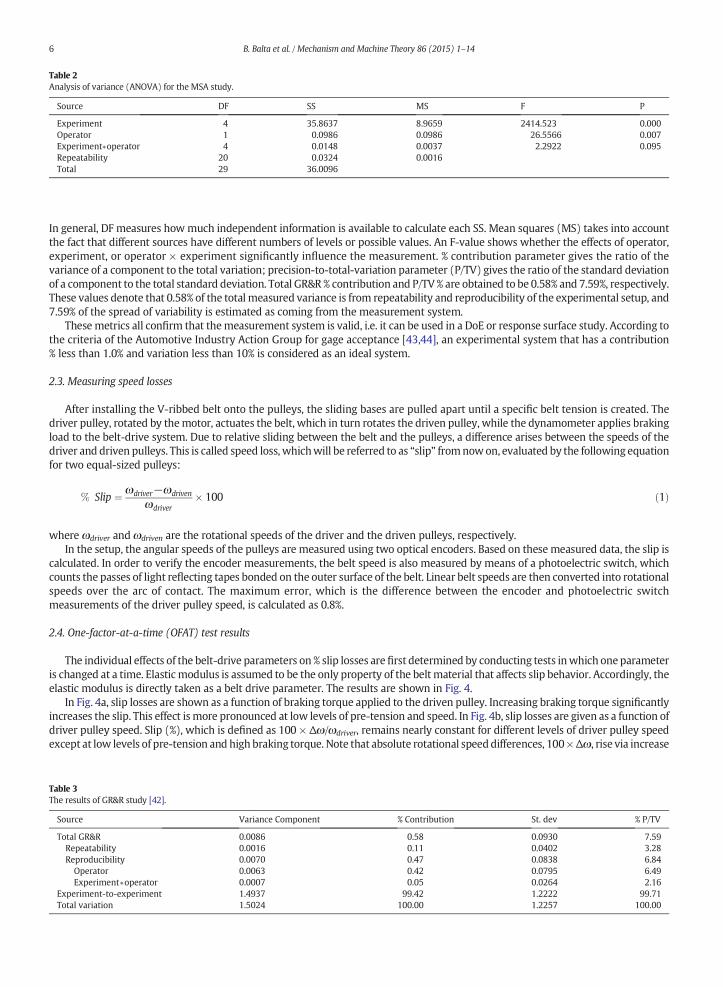
Table 2Analysis of variance (ANOVA) for the MSA study.

Source DF SS MS F P

Experiment 4 35.8637 8.9659 2414.523 0.000Operator 1 0.0986 0.0986 26.5566 0.007Experiment∗operator 4 0.0148 0.0037 2.2922 0.095Repeatability 20 0.0324 0.0016Total 29 36.0096

6 B. Balta et al. / Mechanism and Machine Theory 86 (2015) 1–14

In general, DF measures howmuch independent information is available to calculate each SS. Mean squares (MS) takes into accountthe fact that different sources have different numbers of levels or possible values. An F-value shows whether the effects of operator,experiment, or operator × experiment significantly influence the measurement. % contribution parameter gives the ratio of thevariance of a component to the total variation; precision-to-total-variation parameter (P/TV) gives the ratio of the standard deviationof a component to the total standard deviation. Total GR&R % contribution and P/TV% are obtained to be 0.58% and 7.59%, respectively.These values denote that 0.58% of the total measured variance is from repeatability and reproducibility of the experimental setup, and7.59% of the spread of variability is estimated as coming from the measurement system.

These metrics all confirm that themeasurement system is valid, i.e. it can be used in a DoE or response surface study. According tothe criteria of the Automotive Industry Action Group for gage acceptance [43,44], an experimental system that has a contribution% less than 1.0% and variation less than 10% is considered as an ideal system.

2.3. Measuring speed losses

After installing the V-ribbed belt onto the pulleys, the sliding bases are pulled apart until a specific belt tension is created. Thedriver pulley, rotated by themotor, actuates the belt, which in turn rotates the driven pulley, while the dynamometer applies brakingload to the belt-drive system. Due to relative sliding between the belt and the pulleys, a difference arises between the speeds of thedriver and driven pulleys. This is called speed loss, whichwill be referred to as “slip” fromnowon, evaluated by the following equationfor two equal-sized pulleys:

Table 3The resu

Sourc

TotalRepRepOE

ExperTotal

% Slip ¼ ωdriver−ωdriven

ωdriver� 100 ð1Þ

where ωdriver and ωdriven are the rotational speeds of the driver and the driven pulleys, respectively.In the setup, the angular speeds of the pulleys are measured using two optical encoders. Based on these measured data, the slip is

calculated. In order to verify the encoder measurements, the belt speed is also measured by means of a photoelectric switch, whichcounts the passes of light reflecting tapes bonded on the outer surface of the belt. Linear belt speeds are then converted into rotationalspeeds over the arc of contact. The maximum error, which is the difference between the encoder and photoelectric switchmeasurements of the driver pulley speed, is calculated as 0.8%.

2.4. One-factor-at-a-time (OFAT) test results

The individual effects of the belt-drive parameters on % slip losses arefirst determined by conducting tests inwhich oneparameteris changed at a time. Elastic modulus is assumed to be the only property of the belt material that affects slip behavior. Accordingly, theelastic modulus is directly taken as a belt drive parameter. The results are shown in Fig. 4.

In Fig. 4a, slip losses are shown as a function of braking torque applied to the driven pulley. Increasing braking torque significantlyincreases the slip. This effect ismore pronounced at low levels of pre-tension and speed. In Fig. 4b, slip losses are given as a function ofdriver pulley speed. Slip (%), which is defined as 100 × Δω/ωdriver, remains nearly constant for different levels of driver pulley speedexcept at low levels of pre-tension and high braking torque. Note that absolute rotational speeddifferences, 100×Δω, rise via increase

lts of GR&R study [42].

e Variance Component % Contribution St. dev % P/TV

GR&R 0.0086 0.58 0.0930 7.59eatability 0.0016 0.11 0.0402 3.28roducibility 0.0070 0.47 0.0838 6.84perator 0.0063 0.42 0.0795 6.49xperiment∗operator 0.0007 0.05 0.0264 2.16iment-to-experiment 1.4937 99.42 1.2222 99.71variation 1.5024 100.00 1.2257 100.00

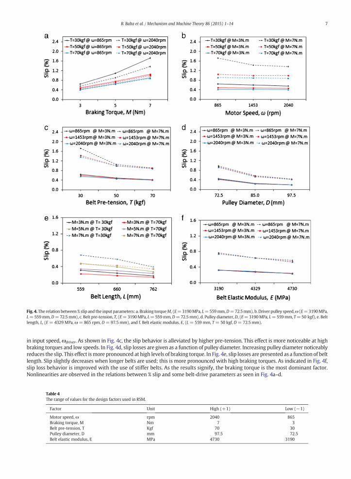
Fig. 4. The relation between % slip and the input parameters: a. Braking torqueM, (E=3190MPa, L=559mm,D=72.5mm), b. Driver pulley speed,ω (E=3190MPa,L=559mm,D=72.5mm), c. Belt pre-tension, T, (E=3190MPa, L=559mm,D=72.5mm), d. Pulley diameter,D, (E=3190MPa, L=559mm, T=50 kgf), e. Beltlength, L, (E = 4329 MPa, ω = 865 rpm, D = 97.5 mm), and f. Belt elastic modulus, E, (L = 559 mm, T = 50 kgf, D = 72.5 mm).

7B. Balta et al. / Mechanism and Machine Theory 86 (2015) 1–14

in input speed, ωdriver. As shown in Fig. 4c, the slip behavior is alleviated by higher pre-tension. This effect is more noticeable at highbraking torques and low speeds. In Fig. 4d, slip losses are given as a function of pulley diameter. Increasing pulley diameter noticeablyreduces the slip. This effect ismore pronounced at high levels of braking torque. In Fig. 4e, slip losses are presented as a function of beltlength. Slip slightly decreases when longer belts are used; this is more pronounced with high braking torques. As indicated in Fig. 4f,slip loss behavior is improved with the use of stiffer belts. As the results signify, the braking torque is the most dominant factor.Nonlinearities are observed in the relations between % slip and some belt-drive parameters as seen in Fig. 4a–d.

Table 4The range of values for the design factors used in RSM.

Factor Unit High (+1) Low (−1)

Motor speed, ω rpm 2040 865Braking torque, M Nm 7 3Belt pre-tension, T Kgf 70 30Pulley diameter, D mm 97.5 72.5Belt elastic modulus, E MPa 4730 3190

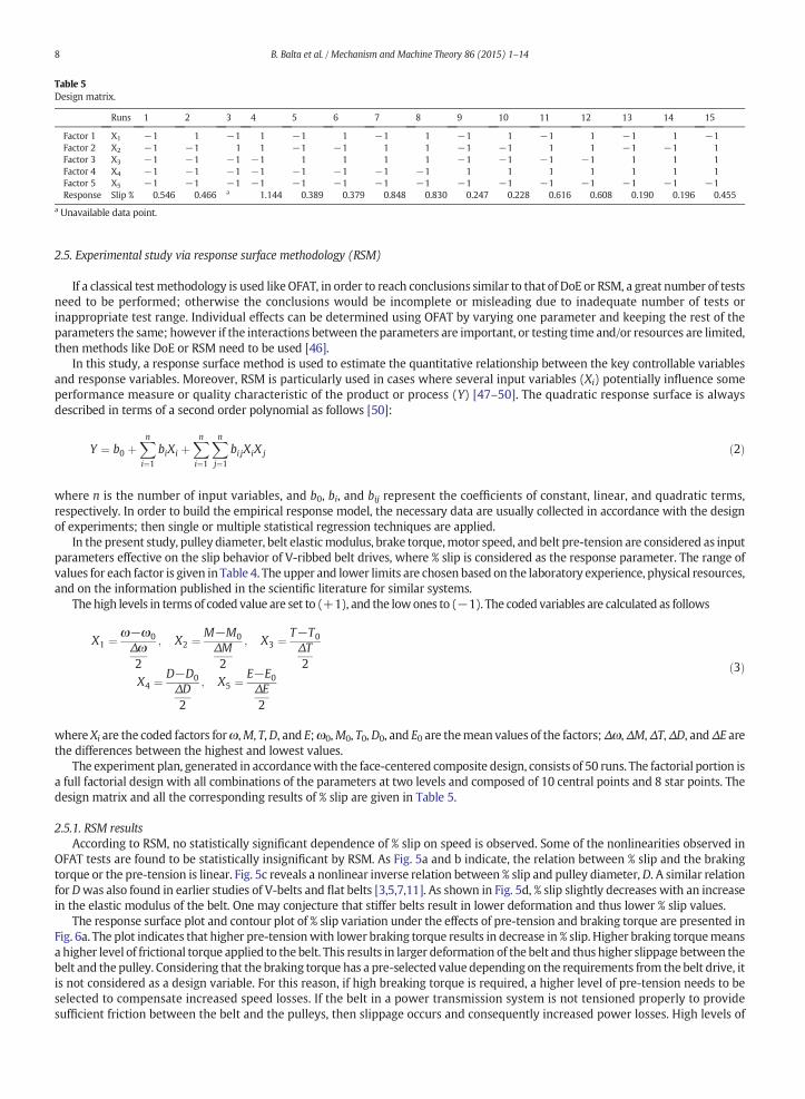
Table 5Design matrix.

Runs 1 2 3 4 5 6 7 8 9 10 11 12 13 14 15

Factor 1 X1 −1 1 −1 1 −1 1 −1 1 −1 1 −1 1 −1 1 −1Factor 2 X2 −1 −1 1 1 −1 −1 1 1 −1 −1 1 1 −1 −1 1Factor 3 X3 −1 −1 −1 −1 1 1 1 1 −1 −1 −1 −1 1 1 1Factor 4 X4 −1 −1 −1 −1 −1 −1 −1 −1 1 1 1 1 1 1 1Factor 5 X5 −1 −1 −1 −1 −1 −1 −1 −1 −1 −1 −1 −1 −1 −1 −1Response Slip % 0.546 0.466 a 1.144 0.389 0.379 0.848 0.830 0.247 0.228 0.616 0.608 0.190 0.196 0.455

a Unavailable data point.

8 B. Balta et al. / Mechanism and Machine Theory 86 (2015) 1–14

2.5. Experimental study via response surface methodology (RSM)

If a classical test methodology is used like OFAT, in order to reach conclusions similar to that of DoE or RSM, a great number of testsneed to be performed; otherwise the conclusions would be incomplete or misleading due to inadequate number of tests orinappropriate test range. Individual effects can be determined using OFAT by varying one parameter and keeping the rest of theparameters the same; however if the interactions between the parameters are important, or testing time and/or resources are limited,then methods like DoE or RSM need to be used [46].

In this study, a response surface method is used to estimate the quantitative relationship between the key controllable variablesand response variables. Moreover, RSM is particularly used in cases where several input variables (Xi) potentially influence someperformance measure or quality characteristic of the product or process (Y) [47–50]. The quadratic response surface is alwaysdescribed in terms of a second order polynomial as follows [50]:

Y ¼ b0 þXn

i¼1

biXi þXn

i¼1

Xn

j¼1

bi jXiX j ð2Þ

where n is the number of input variables, and b0, bi, and bij represent the coefficients of constant, linear, and quadratic terms,respectively. In order to build the empirical response model, the necessary data are usually collected in accordance with the designof experiments; then single or multiple statistical regression techniques are applied.

In the present study, pulley diameter, belt elasticmodulus, brake torque,motor speed, and belt pre-tension are considered as inputparameters effective on the slip behavior of V-ribbed belt drives, where % slip is considered as the response parameter. The range ofvalues for each factor is given in Table 4. The upper and lower limits are chosen based on the laboratory experience, physical resources,and on the information published in the scientific literature for similar systems.

The high levels in terms of coded value are set to (+1), and the lowones to (−1). The coded variables are calculated as follows

X1 ¼ ω−ω0Δω2

; X2 ¼ M−M0ΔM2

; X3 ¼ T−T0ΔT2

X4 ¼ D−D0ΔD2

; X5 ¼ E−E0ΔE2

ð3Þ

where Xi are the coded factors forω,M, T,D, and E;ω0,M0, T0,D0, and E0 are themean values of the factors;Δω,ΔM,ΔT,ΔD, andΔE arethe differences between the highest and lowest values.

The experiment plan, generated in accordancewith the face-centered composite design, consists of 50 runs. The factorial portion isa full factorial design with all combinations of the parameters at two levels and composed of 10 central points and 8 star points. Thedesign matrix and all the corresponding results of % slip are given in Table 5.

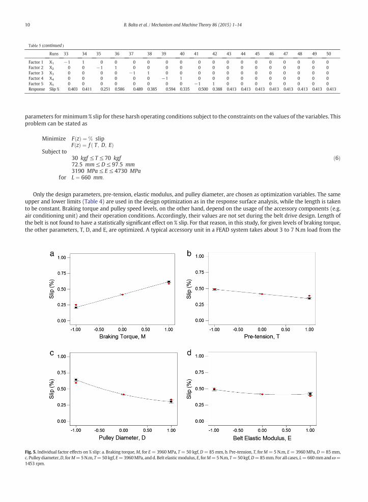
2.5.1. RSM resultsAccording to RSM, no statistically significant dependence of % slip on speed is observed. Some of the nonlinearities observed in

OFAT tests are found to be statistically insignificant by RSM. As Fig. 5a and b indicate, the relation between % slip and the brakingtorque or the pre-tension is linear. Fig. 5c reveals a nonlinear inverse relation between % slip and pulley diameter,D. A similar relationfor Dwas also found in earlier studies of V-belts and flat belts [3,5,7,11]. As shown in Fig. 5d, % slip slightly decreases with an increasein the elastic modulus of the belt. One may conjecture that stiffer belts result in lower deformation and thus lower % slip values.

The response surface plot and contour plot of % slip variation under the effects of pre-tension and braking torque are presented inFig. 6a. The plot indicates that higher pre-tensionwith lower braking torque results in decrease in % slip. Higher braking torquemeansa higher level of frictional torque applied to the belt. This results in larger deformation of the belt and thus higher slippage between thebelt and the pulley. Considering that the braking torque has a pre-selected value depending on the requirements from the belt drive, itis not considered as a design variable. For this reason, if high breaking torque is required, a higher level of pre-tension needs to beselected to compensate increased speed losses. If the belt in a power transmission system is not tensioned properly to providesufficient friction between the belt and the pulleys, then slippage occurs and consequently increased power losses. High levels of

Table 5Design matrix.

16 17 18 19 20 21 22 23 24 25 26 27 28 29 30 31 32

1 −1 1 −1 1 −1 1 −1 1 −1 1 −1 1 −1 1 −1 11 −1 −1 1 1 −1 −1 1 1 −1 −1 1 1 −1 −1 1 11 −1 −1 −1 −1 1 1 1 1 −1 −1 −1 −1 1 1 1 11 −1 −1 −1 −1 −1 −1 −1 −1 1 1 1 1 1 1 1 1

−1 1 1 1 1 1 1 1 1 1 1 1 1 1 1 1 10.447 0.426 0.415 1.100 1.100 0.343 0.335 0.769 0.735 0.203 0.192 0.500 0.463 0.170 0.167 0.403 0.373

9B. Balta et al. / Mechanism and Machine Theory 86 (2015) 1–14

belt tension, on the other hand, have adverse effects. A high tension increases the pulley hub load, which causes premature failure ofthe bearings, while a low tension results in slippage. Fig. 6b shows the effects of the pulley diameter and the braking torque on % slip.Use of a larger pulley diameter combinedwith lower braking torque results in decreased % slip. When the smallest pulley is used andthe braking torque takes itsmaximumvalue, tension difference between the tight side and the slack side of the belt reaches to itsmax-imum level. Therefore, the change in the extension experienced by the belt during its contact with the pulley will be larger. This leadsto a larger creep and thus increased slippage. With smaller pulley sizes, hysteresis losses will also be higher due to a larger change innormal strains and a larger extent of bending and unbending of the belt as it runs over the pulleys. If a high level of braking torque isrequired, a larger pulley diameter is recommended to reduce the power losses. The plot in Fig. 6c presents interactions of the pulleydiameter and the pre-tension in affecting % slip. Smaller pulley diameters together with lower pre-tension result in higher % slip. Asimilar effect is also observed by Childs and Cowburn [11] in V-belt drives. When the belt tension is low, then, the normal forces be-tween the belt and pulley will not be high enough to generate sufficient frictional forces to sustain the transmission. However, as ob-served in Fig. 6c, pre-tension does not have a strong effect on % slip in V-ribbed belt drives as long as gross slippage does not occur.

2.5.2. ANOVAAnalysis of variance (ANOVA) is a commonly used statistical method based on decomposition of the total variability in the

response variable, Y. Using ANOVA, comparisons can bemade between themeans of two ormore parameters in order to differentiatethe effective parameters on the desired response. Table 6 presents the statistical significance of each input variable as well as theinteraction terms on the % slip behavior. If the value of Prob N F is smaller than 0.05, the regression model is considered to bestatistically significant; otherwise the variable does not have a statistically significant effect on the response parameter. Table 6presents only the significant terms obtained by backward elimination. The main factors, quadratic terms as well as the interactionterms shown in Table 6, have Prob N F values less than 0.05; consequently they are considered to be significant. As indicated InTable 6, there is no significant lack of fit in the model, which is expressed by Eq. (4); so it can be concluded that the reduced modelis adequate. The F value of a term reflects the degree of its significance. Highest F values are obtained to be 1642 for the braking torqueand 1122 for the pulley diameter. This means that they are the most effective parameters on the response, i.e. % slip.

The quadratic equation of the response surface model of % slip obtained by regression analysis is given in coded parametersby

Slip %ð Þ ¼ 0:42þ 0:2X2−0:072X3−0:17X4−0:033X5−0:039X2X3−0:065X2X4

þ 0:033X3X4 þ 0:059X24 þ 0:038X2

5:ð4Þ

Furthermore, the value of R2 is obtained to be 98.81% for theRSMmodel. This value indicates that themodelwill predict future dataquite well. R2 is a measure of the strength of the relationship between the experimental data and the predicted values from theregression model and expressed as

R2 ¼ SSRSST

ð5Þ

where SS is the sum of squares; T and R indicate the total model and regression model, respectively.

3. Optimization of design parameters

3.1. Objective function

After finding the functional relationship between the key controllable variables and the response variable, it is possible to optimizethe response. The objective function to be minimized is given in Eq. (4).

3.2. Case study

Speed loss is a critical factor in belt-drive transmissions in which small pulleys are used like front-end accessory drives(FEAD) in automotive vehicles. The optimization problem in this case study is to find the optimal values of the design

Runs 33 34 35 36 37 38 39 40 41 42 43 44 45 46 47 48 49 50

Factor 1 X1 −1 1 0 0 0 0 0 0 0 0 0 0 0 0 0 0 0 0Factor 2 X2 0 0 −1 1 0 0 0 0 0 0 0 0 0 0 0 0 0 0Factor 3 X3 0 0 0 0 −1 1 0 0 0 0 0 0 0 0 0 0 0 0Factor 4 X4 0 0 0 0 0 0 −1 1 0 0 0 0 0 0 0 0 0 0Factor 5 X5 0 0 0 0 0 0 0 0 −1 1 0 0 0 0 0 0 0 0Response Slip % 0.403 0.411 0.251 0.586 0.489 0.385 0.594 0.335 0.500 0.388 0.413 0.413 0.413 0.413 0.413 0.413 0.413 0.413

Fig. 5. Individual factor effects on % slip: a. Braking torque,M, for E=3960MPa, T=50 kgf, D=85mm, b. Pre-tension, T, forM=5 N.m, E=3960MPa, D=85mmc. Pulley diameter,D, forM=5N.m, T=50kgf, E=3960MPa, andd. Belt elasticmodulus, E, forM=5N.m, T=50kgf,D=85mm. For all cases, L=660mmandω=1453 rpm.

Table 5 (continued )

10 B. Balta et al. / Mechanism and Machine Theory 86 (2015) 1–14

parameters for minimum% slip for these harsh operating conditions subject to the constraints on the values of the variables. Thisproblem can be stated as

Minimize F zð Þ ¼ % slipF zð Þ ¼ f T; D; Eð Þ

Subject to30 kgf ≤ T ≤ 70 kgf72:5 mm ≤ D ≤ 97:5 mm3190 MPa ≤ E ≤ 4730 MPa

for L ¼ 660 mm:

ð6Þ

Only the design parameters, pre-tension, elastic modulus, and pulley diameter, are chosen as optimization variables. The sameupper and lower limits (Table 4) are used in the design optimization as in the response surface analysis, while the length is takento be constant. Braking torque and pulley speed levels, on the other hand, depend on the usage of the accessory components (e.g.air conditioning unit) and their operation conditions. Accordingly, their values are not set during the belt drive design. Length ofthe belt is not found to have a statistically significant effect on % slip. For that reason, in this study, for given levels of braking torque,the other parameters, T, D, and E, are optimized. A typical accessory unit in a FEAD system takes about 3 to 7 N.m load from the

,

Fig. 6. Response surface and contour plots of % slip variation vs. a. Pre-tension, T, and braking torque,M, forD=85mm, E=3960MPa, b. Pulley diameter,D, and brakingtorque,M, for T = 50 kgf, E = 3960 MPa, and c. Pulley diameter, D, and pre-tension, T, for M = 5 N.m, E = 3960 MPa. For all cases, L = 660 mm and ω = 1453 rpm.

11B. Balta et al. / Mechanism and Machine Theory 86 (2015) 1–14

crankshaft depending on the power requirements. In this case study, the braking torque levels are then chosen within this range.Optimal settings,whichminimize % slipwithin the selected ranges, are listed in Table 7 in terms of coded values. Depending on typicalusage of the accessory components, one of the optimum settings may be used in belt drive design.

4. Verification of the model

4.1. Confirmation experiments

In order to verify the response surface model, additional tests are performed using the same experimental setup with arbitrarilychosen values for the belt drive parameters. The confirmation experiments reveal that the difference between the predicted valuesfor % slip and the experimental values are smaller than 7%.Onemay conclude that the proposedmodel for % slip in V-ribbedbelt drivesis reasonably accurate.

Table 6ANOVA for % slip (after backward elimination).

Source Sum Degree Mean F value Prob N F

of squares of freedom square

Model 2.5000 9 0.2800 332 b0.0001 SignificantX2 1.3700 1 1.3700 1642 b0.0001X3 0.1700 1 0.1700 204 b0.0001X4 0.9400 1 0.9400 1122 b0.0001X5 0.0360 1 0.0360 43 b0.0001X2·X3 0.0470 1 0.0470 56 b0.0001

Std. dev. 0.0290 X2·X4 0.1300 1 0.1300 156 b0.0001Mean 0.4700 X3·X4 0.0330 1 0.0330 39 b0.0001C.V. % 6.1700 X4

2 0.0120 1 0.0120 15 0.0004PRESS 0.0570 X5

2 0.0053 1 0.0053 6 0.0157R-squared 0.9881 Residual 0.0330 39 0.0008Adj. R-squared 0.9842 Lack of fit 0.0330 32 0.0010 Not significantPred. R-squared 0.9776 Pure error 0.0000 7 0.0000Adeq. precision 73.4640 Cor. total 2.5300 48

Table 7Optimal settings for minimal % slip for given levels of braking torque.

Set levels Optimal levels

Braking torque Pre-tension Pulley diameter Elastic modulus Slip (%)

−1.00 0.99 0.90 0.90 0.160.00 1.00 1.00 0.48 0.261.00 1.00 1.00 0.44 0.36

12 B. Balta et al. / Mechanism and Machine Theory 86 (2015) 1–14

4.2. Correlation with the results in the literature

In some of the previous studies, similar belt-drive systems were used and the slip was measured for different testconditions. Table 8 presents % slip values measured by Yu [29] and the predictions of the RSM model given in Eq. (4). The results ofthe model developed in the present study are in good agreement with the empirical data provided by Yu [29]. The experimentswere conducted in that study with the following test conditions: Pulley diameter = 80 mm, motor speed = 1000 rpm, andpre-tension= 42.83 kgf. Because the elastic modulus of the belt used in the experiments was not given in the reference, the mediumvalue is used for the belt elastic modulus in the calculations. The results correlate well even though some of the values of brakingtorque are outside the limits chosen for the braking torque in the present study.

5. Model adequacy check

In order to ensure that the models have extracted all the relevant information from the experimental data, the adequacy of theexperimental design is examined. The residual analysis is the primary diagnostic tool for this purpose [43,44,46]. Residual is definedas the difference between the actual and predicted values of the response for a given design. The results of the residual analysis areshown in Fig. 7a, b, and c.

First of all, for an adequate model, the residuals should have normal distribution regardless of whether the response has a normaldistribution or not. The vertical axis of Fig. 7a is the probability scale and the horizontal axis is the data scale. A least-square line isfitted to the plotted points. The line forms an estimate of the cumulative distribution function for the population from which dataare drawn. The P-value for the data shown in Fig. 7a is larger than 0.05, thus, the residuals for % slip values follow a normal distribution.

Fig. 7b represents the fitted value plot, where the values of % slip predicted by the response curve are on the horizontal axis and thedifferences between the actual and predicted values are on the vertical axis. The fitted value plot should represent equal variancelevels around the center line, which corresponds to zero residual value, as shown in Fig. 7b.

Fig. 7c represents the order of the data plot, where the data are given in the observed order on the horizontal axis and the residualvalues are given on the vertical axis similar to the fitted value plot. Themeasurements should not affect subsequentmeasurements orthe setup should not produce data showing any significant trend over time. Themeasured data in the present study can be consideredto be adequate in this respect. From thesefigures, onemay conclude that the predictive regressionmodel obtained at thefinal stage ofthe study is adequate in the sense that the basic assumptions of the regression analysis like errors being uncorrelated are correct.

6. Conclusions

In this study, a test setup is developed to determine the effects of pulley diameter, pulley speed, belt length, belt pre-tension, beltmaterial, and braking torque on % slip (% speed loss) in V-ribbed belt drives. One-factor-at-a-time (OFAT) and response surface testmethodologies are used to find the relation between belt-drive parameters and % slip.

Slipmeasurements on the V-ribbed belt drive system reveal that the smaller is the pulley size, the larger is the belt slip. Experimentalanalysis shows that below a certain level of belt pre-tension, slip values increase rapidly under all types of test conditions. This may beexplained as poor fit between the belt and the pulley grooves. Increasing the braking torque causes a significant increase in slip. Thiseffect is alleviated by high pre-tension. Although the absolute value of slip increases with an increase in driver pulley speed, % slipremains almost constant. When stiffer belts are used, % slip is slightly reduced.

RSM study clearly shows that the belt drive parameters have interactions among themselves and some of the relations betweenthe belt-drive parameters and % slip are nonlinear. Response surface plots distinctly indicate the effective parameters and the natureof their effects on the % slip.

Table 8The correlation of RSM results with previously reported experimental data.

Braking torque(N.m)

RSMSlip (%)

Yu [29]Slip (%)

Difference(%)

2.5 0.22 0.20 9.16.8 0.75 0.70 6.710.5 1.20 1.15 4.2

Fig. 7.Adequacy check for the response surface design: a. Normal distribution plot of the residuals, b. Fitted value plot for % slip, and c. Observation order plot of residualsfor % slip.

13B. Balta et al. / Mechanism and Machine Theory 86 (2015) 1–14

The adequacy of the RSMmodel is checked and verified via ANOVA. Besides, experiments are conducted with arbitrary operatingconditions; then the measured values of % slip and the values predicted by RSM are compared. The comparison indicates that theerrors are smaller than 7%. The predictions of the formulation are also found to be in good agreement with the results of a previousexperimental study in the literature.

Usuallymotor speed and braking torque have pre-defined values at the beginning of a belt drive design. In this study, the optimumoperating conditions are found for preselected values of braking torque by minimizing the function for % slip derived by RSM.

Acknowledgments

We would like to thank Assoc. Prof. Dr. Mehmet Uçar and Bülent Balta, for their valuable support to this study. We would like tothank Teklas A.Ş. where stiffness measurements are performed.

References

[1] A. Almeida, S. Greenberg, Technology assessment: energy-efficient belt transmissions, Energy Build. 22 (3) (1995) 245–253.[2] O. Reynolds, On the efficiency of belts or straps as communicators of work, Engineering 38 (1874) 396.[3] G. Gerbert, On flat belt slip, Veh. Tribol. Ser. 16 (1991) 333–339.[4] K.L. Johnson, Contact Mechanics, first ed. Cambridge University Press, London, 1987.[5] T.C. Firbank, Mechanics of the belt drive, Int. J. Mech. Sci. 12 (1970) 1053–1063.[6] G. Gerbert, Some notes on V-belt drives, J. Mech. Des. 103 (1981) 8–18.[7] G. Gerbert, Belt slip-a unified approach, J. Mech. Des. 118 (1996) 432s–438s.[8] F. Sorge, G. Gerbert, Full sliding “adhesive-like” contact of V-belts, ASME J. Mech. Des. 124 (4) (2002) 706–712.[9] H. Peeken, F. Fischer, Experimental investigation of power loss and operating conditions of statically loaded belt drives, Proceedings of the 1989 International

Power Transmission and Gearing Conference, Illinois, 1989, pp. 15–24.[10] T.H.C. Childs, D. Cowburn, Power transmission losses in V-belt drives, Part 1: mismatched belt and pulley groove wedge angle effects, Proc. Inst. Mech. Eng. D J.

Automob. Eng. 201 (1987) 33–40.[11] T.H.C. Childs, D. Cowburn, Power transmission losses in V-belt drives, Part 2: effects of small pulley radii, Proc. Inst. Mech. Eng. D J. Automob. Eng. 201 (1987)

41–53.[12] V.A. Lubarda, Determination of the belt force before the gross slip, Mech. Mach. Theory 83 (2015) 31–37.[13] F. Ferrando, F. Martin, C. Riba, Axial force test and modeling of the V-belt continuously variable transmission for mopeds, J. Mech. Des. 118 (1996) 266–273.[14] S. Amijma, T. Fujii, H. Matuoka, E. Ikeda, Study on axial force and its distribution for a newly developed block-type CVT belt, Int. J. Veh. Des. 12 (1991) 324–335.[15] T.F. Chen, D.W. Lee, C.K. Sung, An experimental study on transmission efficiency of a rubber V-belt CVT, Mech. Mach. Theory 33 (1998) 351–363.[16] S. Akehurst, N.D. Vaughan, D.A. Parker, D. Simmer, Modeling of loss mechanisms in a pushing metal V-belt continuously variable transmission. Part 1: torque

losses due to band friction, Proc. Inst. Mech. Eng. D J. Automob. Eng. 218 (11) (2004) 1269–1281.

14 B. Balta et al. / Mechanism and Machine Theory 86 (2015) 1–14

[17] S. Akehurst, N.D. Vaughan, D.A. Parker, D. Simmer, Modeling of loss mechanisms in a pushing metal V-belt continuously variable transmission. Part 2: pulleydeflection losses and total torque loss validation, Proc. Inst. Mech. Eng. D J. Automob. Eng. 218 (11) (2004) 1283–1293.

[18] S. Akehurst, N.D. Vaughan, D.A. Parker, D. Simmer, Modeling of loss mechanisms in a pushing metal V-belt continuously variable transmission. Part 3: belt sliplosses, Proc. Inst. Mech. Eng. D J. Automob. Eng. 218 (11) (2004) 1295–1306.

[19] L. Bertini, L. Carmignani, F. Frendo, Analytical model for the power losses in rubber V-belt continuously variable transmission (CVT), Mech. Mach. Theory 78(2014) 289–306.

[20] G. Mantriota, Theoretical and experimental study of a power split continuously variable transmission system, Part 1, Proc. Inst. Mech. Eng. D J. Automob. Eng. 215(2001) 837–850.

[21] G. Mantriota, Theoretical and experimental study of a power split continuously variable transmission system, Part 2, Proc. Inst. Mech. Eng. D J. Automob. Eng. 215(2001) 851–864.

[22] G. Mantriota, Power split continuously variable transmission systems with high efficiency, Proc. Inst. Mech. Eng. D J. Automob. Eng. 215 (2001) 357–368.[23] G. Mantriota, E. Pennestri, Theoretical and experimental efficiency analysis of multi-degrees-of-freedom epicyclic gear trains, Multi-Body Syst. Dyn. 9 (2003)

389–408.[24] G. Carbone, L. Mangialardi, B. Bonsen, C. Tursi, P.A. Veenhuizen, CVT dynamics: theory and experiments, Mech. Mach. Theory 42 (2007) 409–428.[25] G. Carbone, L. Mangialardi, G. Mantriota, The influence of pulley deformations on the shifting mechanism of metal belt CVT, J. Mech. Des. 127 (2005) 103–113.[26] C. Zhu, H. Liu, J. Tian, W. Xiao, X. Du, Experimental investigation on the efficiency of the pulley-drive CVT, Int. J. Automot. Technol. 11 (2) (2010) 257–261.[27] K.W. Dalgarno, R.B. Moore, A.J. Day, Tangential slip noise of V-ribbed belts, Proc. Inst. Mech. Eng. C J. Mech. Eng. Sci. 213 (1999) 741–749.[28] D. Yu, T.H.C. Childs, K.W. Dalgarno, Experimental and finite element studies of the running of V-ribbed belts in pulley grooves, Proc. Inst. Mech. Eng. C J. Mech.

Eng. Sci. 212 (1998) 343–355.[29] D. Yu, Slip of the four belts, Fig. 4.6a, 87(PhD Thesis) Mechanical performance of automotive V-ribbed belts, Department of Mechanical Engineering, The

University of Leeds, UK1996.[30] D. Yu, T.H.C. Childs, K.W. Dalgarno, V-ribbed belt design, wear and traction capacity, Proc. Inst. Mech. Eng. D J. Automob. Eng. 212 (1998) 333–344.[31] M. Xu, J.B. Castle, Y. Shen, K. Chandrashekhara, Finite element simulation and experimental validation of V-ribbed belt tracking, SAE 2001World Congress, 2001,

2001. Paper No. 2001-01-0661.[32] L. Manin, G. Michon, D. Remond, R. Dufour, From transmission error measurement to pulley-belt slip determination in serpentine belt drives: influence of

tensioner and belt characteristics, Mech. Mach. Theory 44 (2009) 813–821.[33] G. Cepon, L. Manin, M. Boltezar, Experimental identification of the contact parameters between a V-ribbed belt and pulley, Mech. Mach. Theory 45 (2010)

1424–1433.[34] G. Cepon, L. Manin, M. Boltezar, Introduction of damping into the flexible multibody belt-drive model: a numerical and experimental investigation, J. Sound Vib.

324 (2009) 283–296.[35] G. Cepon, M. Boltezar, An advanced numerical model for dynamic simulations of automotive belt-drives, 2010. SAE 2010-01-1409.[36] L. Pietra, F. Timpone, Tension in a flat belt transmission: experimental investigation, Mech. Mach. Theory 70 (2013) 129–156.[37] R.R. Senthilkumar, K. Sooryaprakash, Industrial drive belt tensioning optimization, International Conference on Current Trends in Engineering and Technology,

IEEE-32107, ICCTET, 2013, ISBN 978-1-4799-2585-8. 304–306 (Coimbatore, India), IEEE Catalogue Number:CFP1300W-POD.[38] G. Gerbert, A note on slip in V-belt drives, J. Eng. Ind. Trans. (1976) 1366–1368.[39] H. Belofsky, On the theory of power transmission by V-belts, Wear 39 (1976) 263–275.[40] W. Chen, C. Shieh, On angular speed loss analysis of flat belt transmission system by finite element method, Int. J. Comput. Eng. Sci. 4 (2003) 1–18.[41] S.J. Zhang, Z. Wan, G.L. Liu, Global optimization design method for maximizing the capacity of V-belt drive, Sci. China Technol. Sci. 54 (1) (2010) 140–147.[42] B. Balta, F.O. Sönmez, A.K. Cengiz, Gage repeatability and reproducibility investigations of a test rig using Anova/Xbar-R method, ASME, International Mechanical

Engineering Conference, Paper No. IMECE2011-62130, 3, 2011, pp. 793–800.[43] F.W. Breyfogle III, Implementing Six Sigma, Smarter Solutions Using Statistical Methods, second ed. John Wiley & Sons, New York, 2003.[44] The Black Belt Memory Jogger, first ed. GOAL/QPC and SixSigma Academy, 2002.[45] Measurement System Analysis, Reference Manual, fourth ed. ChryslerGroup LLC, Ford Motor Company, General Motors Corporation, June 2010.[46] D.C. Montgomery, Design and Analysis of Experiments, fifth ed. Wiley Series in Probability and Statistics, New York, 2001.[47] C. Chen, P. Su, Y. Lin, Analysis and modeling of effective parameters for dimension shrinkage variation of injection molded part with thin shell feature using

response surface methodology, Int. J. Adv. Manuf. Technol. 45 (2009) 1087–1095.[48] U. Reisgen, M. Schleser, O. Mokrov, E. Ahmed, Statistical modeling of laser welding of DP/TRIP steel sheets, Opt. Laser Technol. 44 (2012) 92–101.[49] U. Reisgen, M. Schleser, O. Mokrov, E. Ahmed, Optimization of laser welding of DP/TRIP steel sheets using statistical approach, Opt. Laser Technol. 44 (2012)

255–262.[50] R.H. Myers, D.C. Montgomery, Response Surface Methodology, second ed. Wiley Series in Probability and Statistics, New York, 2002.