ME 303 FLUID MECHANICS I

Prof. Dr. Haşmet Türkoğlu

Çankaya University Faculty of Engineering

Mechanical Engineering Department

Fall, 2016

2

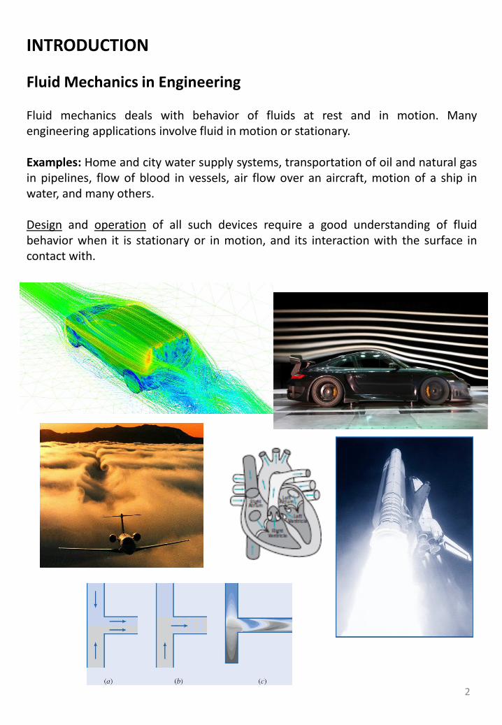
INTRODUCTION

Fluid Mechanics in Engineering

Fluid mechanics deals with behavior of fluids at rest and in motion. Manyengineering applications involve fluid in motion or stationary.

Examples: Home and city water supply systems, transportation of oil and natural gasin pipelines, flow of blood in vessels, air flow over an aircraft, motion of a ship inwater, and many others.

Design and operation of all such devices require a good understanding of fluidbehavior when it is stationary or in motion, and its interaction with the surface incontact with.

3

Definition of a Fluid

Consider imaginary chunks of both a solid and a fluid. Chunks are fixed along oneedge, and a shear force is applied at the opposite edge.

A short time after application of the force, the solid assumes a deformed shapewhich can be measured by the angle 1. If we maintain this force and examine thesolid at later times, we find that deformation is exactly the same, that is 2= 3 =1.On application of a shear force, a solid assumes a certain deformed shape andretains that shape as long as the same force is applied.

Consider the response of the fluid to the applied shear force. A short time afterapplication of the force, a fluid assumes a deformed shape, as indicated by the angle1. At a later time, the deformation is greater, 2>1, in fact the fluid continues todeform as long as the force is applied.

A fluid is a substance that deforms continuously under the action of an applied shearforce. The process of continuous deformation is called flow.

Scope of Fluid Mechanics

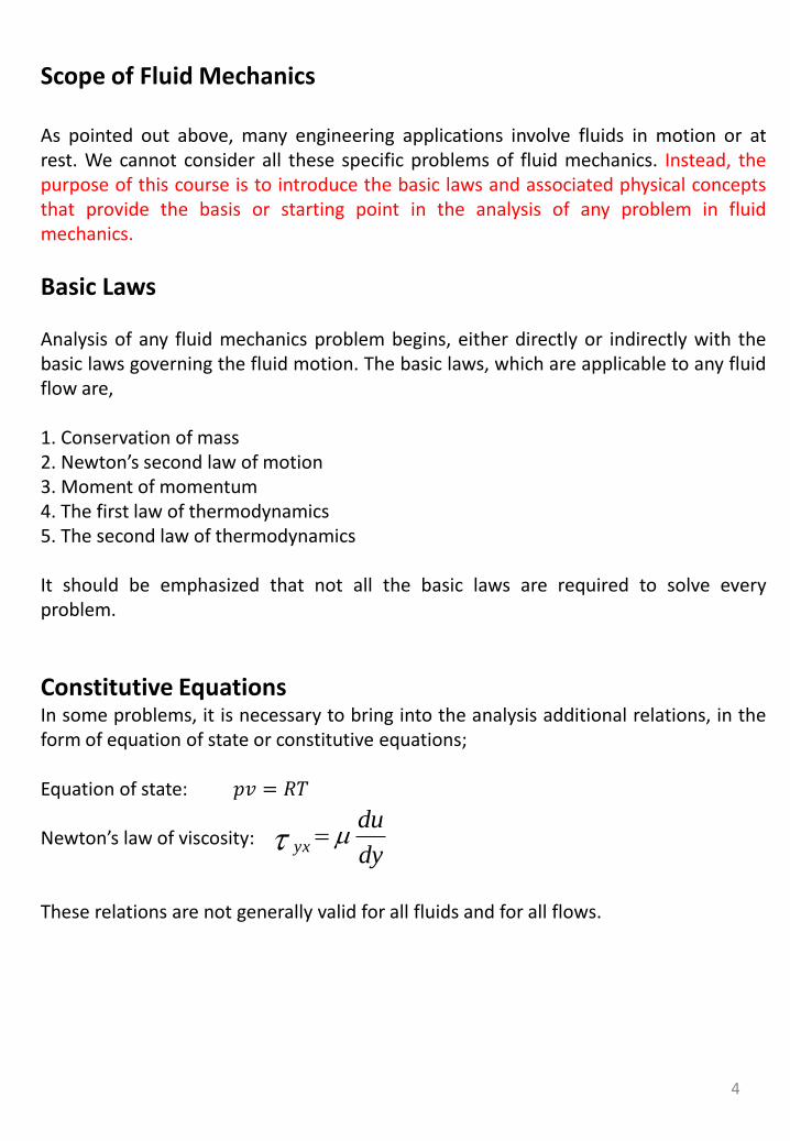
As pointed out above, many engineering applications involve fluids in motion or atrest. We cannot consider all these specific problems of fluid mechanics. Instead, thepurpose of this course is to introduce the basic laws and associated physical conceptsthat provide the basis or starting point in the analysis of any problem in fluidmechanics.

Basic Laws

Analysis of any fluid mechanics problem begins, either directly or indirectly with thebasic laws governing the fluid motion. The basic laws, which are applicable to any fluidflow are,

1. Conservation of mass2. Newton’s second law of motion3. Moment of momentum4. The first law of thermodynamics5. The second law of thermodynamics

It should be emphasized that not all the basic laws are required to solve everyproblem.

Constitutive EquationsIn some problems, it is necessary to bring into the analysis additional relations, in theform of equation of state or constitutive equations;

Equation of state: 𝑝𝑣 = 𝑅𝑇

Newton’s law of viscosity:

These relations are not generally valid for all fluids and for all flows.

4

dy

duyx

Control Volume

A control volume is an arbitrary volume in space through which fluid flows.

Cflow

Control surface

Differential vs Integral Approach

The basic laws that we apply in fluid mechanics problems can be formulated in differential and integral forms. The solution of differential equations provides a means of determining the detailed (point by point) behavior of the fluid.

METHOD OF ANALYSIS

The basic laws can be applied to a control volume or to a system.The first step in solving a problem is to define the system that is going to be analyzed.

System and Control Volume

Gas

A system is defined as a fixed, identifiable quantity of mass.

The boundaries of a system may be fixed ormoveable; however, there is no mass transferacross the system boundaries; i.e. the amountof mass in the system is fixed.

5

The Systems of Dimensions

1) [M], [L], [t], and [T]2) [F], [L], [t], and [T]3) [F],[M], [L], [t], and [T]

Systems of UnitsMLtT

SI (kg, m, s, K)FLtT

British Gravitational (lbf, ft, s, oR)FMLtT

English Engineering (lbf, lbm, ft, s, oR)

Preferred Systems of Units

SI (kg, m, s, K)

British Gravitational (lbf, ft, s, oR)

6

1 N ≡ 1 kg . m/s2

1 slug ≡ 1 lbf . S2/ft

1 slug ≡ 32.2 lbm

FUNDANENTAL CONCEPTS

Topics- Fluid as a Continuum- Velocity Field- Stress Field- Viscosity- Surface Tension- Description and Classification of Fluid Motions

7

FUNDAMENTAL CONCEPTS

Fluid as a Continuum

All fluids are composed of molecules in constant motion. However, in mostengineering applications we are interested in the average or macroscopic effects ofmany molecules. We thus treat a fluid as an infinitely divisible substance, acontinuum, and do not concern with the behavior of individual molecule.

For continuum model to be valid, the smallest sample of the matter of practicalinterest must contain a large number of molecules so that meaningful averages canbe calculated.

The condition for the validation of continuum approach is that distance between themolecules of the fluid should be smaller than the smallest characteristic length of theproblem.

As a consequence of the continuum assumption, fluid properties and flow variablescan be expressed as continuous functions of position and time, i.e.

= (x,y,z,t)u = u (x,y,z,t)T = T (x,y,z,t)p = p (x,y,z,t)…

The value of a fluid property at a point is defined as an average considering a volume around that point.

8

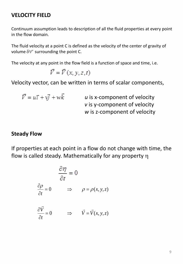
VELOCITY FIELD

Continuum assumption leads to description of all the fluid properties at every point in the flow domain.

The fluid velocity at a point C is defined as the velocity of the center of gravity of volume surrounding the point C.

The velocity at any point in the flow field is a function of space and time, i.e.

Velocity vector, can be written in terms of scalar components,

u is x-component of velocityv is y-component of velocityw is z-component of velocity

Steady Flow

If properties at each point in a flow do not change with time, the flow is called steady. Mathematically for any property

),,(0

),,(0

zyxVVt

V

zyxt

9

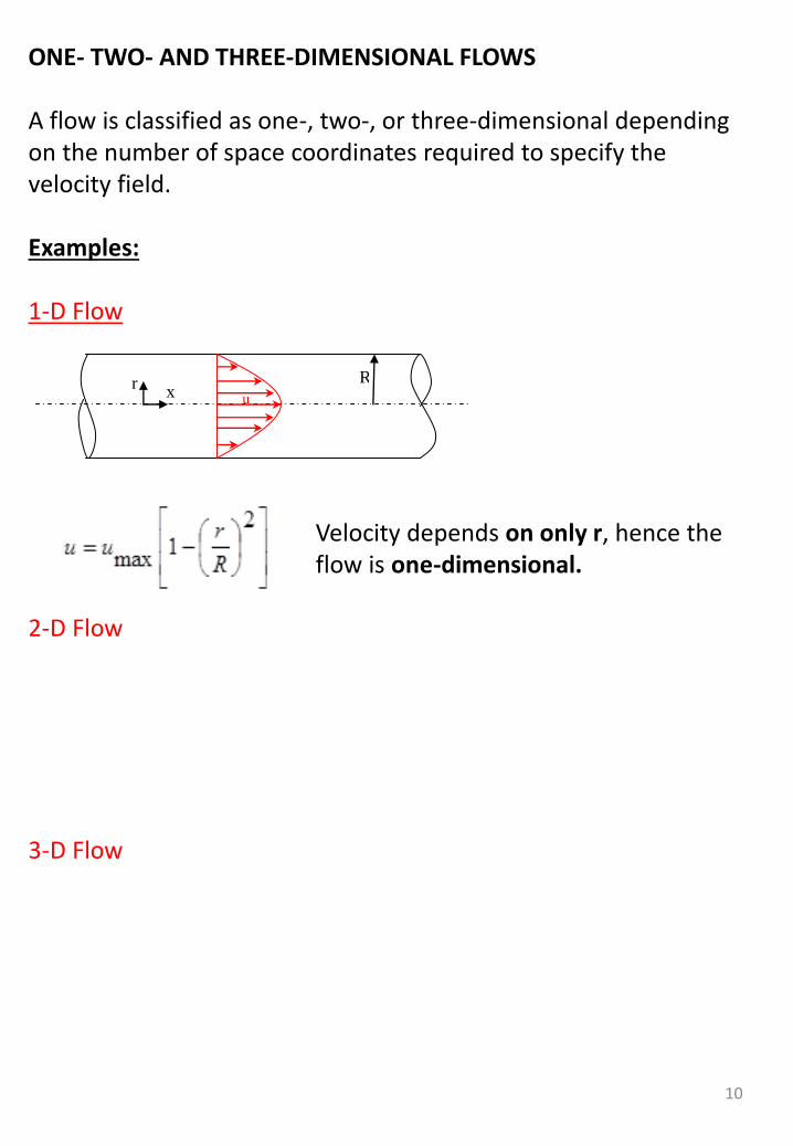
ONE- TWO- AND THREE-DIMENSIONAL FLOWS

A flow is classified as one-, two-, or three-dimensional depending on the number of space coordinates required to specify the velocity field.

Examples:

1-D Flow

u r

x R

Velocity depends on only r, hence the flow is one-dimensional.

2-D Flow

3-D Flow

10

Uniform Flow

To simplify the analysis, sometimes velocity at a cross-section is assumed to beconstant. If velocity at a given cross section is assumed to be uniform, flow is calleduniform flow.

At a given cross section, velocity is the same at all points.

11

Timelines, Pathlines, Streaklines, and Streamlines

Timelines, pathlines, streaklines and streamlines provide a visual representation of a flow field (motion of fluid particles).

Timeline:

If a number of adjacent fluid particles in a flow field are marked at a given instant, they form a line in the fluid at that instant, this line is called a timeline. Observation of the timeline at a later instant may provide information about the flow field.

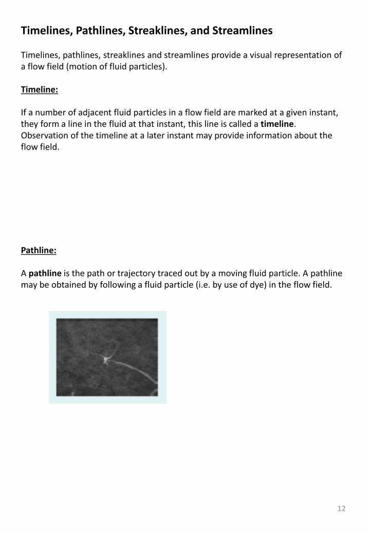
Pathline:

A pathline is the path or trajectory traced out by a moving fluid particle. A pathlinemay be obtained by following a fluid particle (i.e. by use of dye) in the flow field.

12

Streakline:

A line joining the fluid particles that pass through the same point in the flow field is called the streakline.

Streamline:

Streamlines are lines drawn in the flow field so that at given instant they are tangent to the direction of flow at every point in the flow field. Streamlines are tangent to the velocity vector at every point in the flow field.

In steady flows, pathlines, streaklines, and streamlines are identical lines in the flow field.

13

Example: A velocity given by , the units of velocity arem/s; and x and y are given in meters; a=0.1 sec-1.a) Determine the equation for the streamline passing throughthe point

(x0, y0, 0)=(2, 8, 0)b) Determine the velocity of a particle at the point (2, 8, 0)c) If the particle passing through the point (x0, y0, 0) is marked attime t0=0, determine the location of the particle at time t=20 sec.d) What is the velocity of the particle at t=20 sec.e) Show that the equation of the pathline is the same as theequation of the streamline.

14

jayiaxV

15

STRESS FIELD

Forces acting on a fluid element - Surface forces- Body forces

Surface forces include all forces acting on the boundaries of a medium through direct contact.

- Pressure force- Friction (viscous) force

Forces developed without physical contact, and distributed over the volume of the fluid are called body forces.

- Gravitational force- Electromagnetic force

Gravitational body force acting on a fluid element of volume d isand gravitational body force acting on per unit volume of a fluid element is

The concept of stress field provides a convenient means to describe forcesacting on boundaries of a fluid medium and transmitted through themedium.

16

STRESS FIELD

Consider an area A around point C in a continuum. The force acting on can be resolved into two components, one normal and the other tangential to the area

Normal stress sn and shear stress n are defined as

n̂

Fn

Ft Fn

C

F

Note: subscript, n, indicates that the stresses are associated with aparticular surface whose normal vector is n.

Note that at a point C in a continuum different surfaces can be drawn.However, for purpose of analysis, we usually reference the area to somecoordinate system. In rectangular coordinate system, we might considerthe stress components acting on planes whose outward drawn normalvectors are in x, y or z-directions.

17

Force and stress components on area element Ax can be shown as

Stress components shown in above figure is defined as

sxx =

We have used a double subscript notation to label the stresses.i,j

i: indicates plane on which stress acts (axis perpendicular to plane on which stress acts)

j: direction in which stress acts

Consideration of an area element, Ay, would lead to the definition of stresses syy, yx, yz, and use of area element Az would similarly lead to the definitions of szz, zx, zy.

18

xz

sxx

x

y

z

xy

yz

yx

syy

szz

zx

zy

An infinite number of planes can be passed through point C, resulting an infinite number of stresses associated with that point. Fortunately state of stress at a point can be described completely by specifying the stresses acting on three mutually perpendicular planes passing through the point. Hence, stress at a point is specified by the nine components.

zzzyzx

yzyyyx

xzxyxx

s

s

s

The planes are named in terms of the coordinate axes. The planes are named and denoted as positive or negative according to the direction of the outward drawn normal to the plane. Thus, the top plane for example is a positive y-plane and the back plane is a negative z-plane.

It is also necessary to adopt a sign convention for stresses. A stress component is considered positive when the direction of the stress component and the plane on which it acts are both positive or both negative.

Thus, yx=2.4 N/m2 represents a shear stress on positive y-plane in positive x-direction or shear stress on negative y-plane in negative x-direction.

19

VISCOSITYWe have learned that a fluid is a substance that undergoes continuous deformation when subjected to a shear stress. This shear stress is function of rate of deformation. For many common fluids, the shear stress is proportional to the rate of deformation. The constant of proportionality, called viscosity, is a fluid property.

To develop the defining equation for viscosity, we consider a flow in x-yplane in which x-direction velocity varies with y.

Fluid

element

y x

y

x u

δydy

duu

e

Fluid element at time t Fluid element at time t+t

u

Consider the fluid element in the figure. The top of the fluid element moves faster than the bottom, so in time fluid element deforms.

We measure shear deformation by the angle , which can be related to the fluid velocity.

e =

Hence, shear stress is Based on the relation between shear stress and rate of deformation, fluids are grouped as

- Newtonian fluid- Non-Newtonian fluid

20

Newtonian FluidFluid in which constant of proportionality in the above expression is equal to the viscosity called Newtonian fluid.

Examples:

Newton’s law of viscosity:

: dynamic viscosity (absolute viscosity)

Unit of

(Dimension of dynamic viscosity)

tdy

du

L

F

1:

:2

2:L

Ft

Kinematic Viscosity,

sec,,

22 m

t

L

sec

2cmstokeIn metric system sec

0001.012m

poise

dy

duyx

2

sec:

m

N

sec.:m

kg

sec.cm

gpoise

sec1.01

m

kgpoise

In SI system:

In metric system:

21

Non-Newtonian FluidNot all fluids follow the Newton’s law of viscosity (stress-strainrelation). Such fluids are called non-Newtonain. Some fluids such asketchup, are ‘shear-thinning’; that is the coefficient of resistancedecreases with increasing strain rate (it all comes out of the bottle atonce). Others, such as a mixture of sand and water ‘shear-thickening’.Some fluids do not begin to flow until a finite stress been applied(toothpaste).

In these fluids, shear stress-deformation rate (shear strain) relationmay be represented by the power law model,

n

yx dy

duk

n: flow behavior index, k: consistency index

If the above equation is written in the form

dy

du

dy

du

dy

duk

n

yx

1

1

n

dy

duk is referred to as the apparent viscosity.

22

Classification of Non-Newtonian Fluids

Based on the variation of apparent viscosity with rate of deformation, non-Newtonian fluids are classified as follows:

Pseudoplastic Fluid (Shear thinning): Apparent viscosity decreases with increasing deformation rate.Example: polymer solutions, ketchup

Dilatant (Shear thickening): Apparent viscosity increases with increasing deformation rate.Example: sand suspension

Bingham plastic: Deformation (flow) does not begin until a finite stress is applied.Example: toothpaste, drilling muds, clay suspensions

Based on the variation of apparent viscosity in time under constant shear stress:Rheopectic fluid: Apparent viscosity increases with time under constant shear stress.Example: Plaster, cement

Thixotropic fluid: Apparent viscosity decreases with time under constant shear stress. Example: paints

Viscoelastic fluid: Fluid which partially returns to original shape when the applied stress is released. Example: Jelly

23

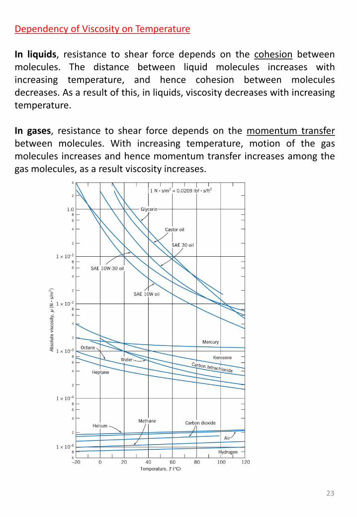
Dependency of Viscosity on Temperature

In liquids, resistance to shear force depends on the cohesion betweenmolecules. The distance between liquid molecules increases withincreasing temperature, and hence cohesion between moleculesdecreases. As a result of this, in liquids, viscosity decreases with increasingtemperature.

In gases, resistance to shear force depends on the momentum transferbetween molecules. With increasing temperature, motion of the gasmolecules increases and hence momentum transfer increases among thegas molecules, as a result viscosity increases.

24

Expample: Consider a fluid flowing on an inclined surface. Its velocity profile is given by

2

2)(Y

y

Y

yUyu

Find shear stress at y=0, Y/2 and Yq

UY

g

width, w

y

x

Solution:

25

COMPRESSIBILITY OF FLUIDS

Bulk Modulus

Pressure and density of liquids are related by the bulk compressibility modulus or modulus of elasticity.

𝐸𝑣 = −𝑑𝑃

𝑑∀/∀𝑜𝑟 𝐸𝑣 =dP/(d/)

Where dP is the differential change in pressure needed to create a differential changedV in volume V (or differential change d in density ).

For water: Ev = 2.15×109 N/m2

Large values of bulk modulus indicate that the fluid is incompressible. That is it takes alarge pressure change to create a change in volume (or in density).

Compression and Expansion of Gases

When gases are compressed (or expanded) the relationship between pressure anddensity (volume) depends on the nature of the process.

If the compression or expansion takes place under constant temperature conditions(isothermal process), then the ideal gas equation (equation of state) becomes

𝑃 = 𝑅𝑇𝑃

𝜌= constant

If the compression or expansion is frictionless and no heat is exchanged with the surroundings (isentropic process) then

𝑃

𝜌𝑘= constant

Where k is the specific heat ratio, k=Cp/Cv

26

Speed of Sound

The velocity at which small disturbunces (the pressure wave of infinitesimal strength) propagate in a medium ( fluid) is called the acoustic velocity or speed of sound.

The peed of sound is is and important characteristic parameter for compresible flows. The speed of sound is related to changes in pressure and density of the fluid medium by the equation:

c = 𝑑𝑃

𝑑

or in terms of bulk modulus c = 𝐸𝑣

For gases undergoing an isentropic process, Ev = kP. Hence, c = 𝑘𝑃

For ideal gases it follows 𝑐 = 𝑘𝑅𝑇

For air at 20 C, speed of sound c = 343 m/s.

For water at 20 C, Ev = 2.15×109 N/m2 and = 998.2 kg/m3 hence speed of sound is obtained as c = 1481 m/s.

If a fluid were truly incompressible (Ev = ), the speed of sound would be infinite.

27

Surface Tension, s

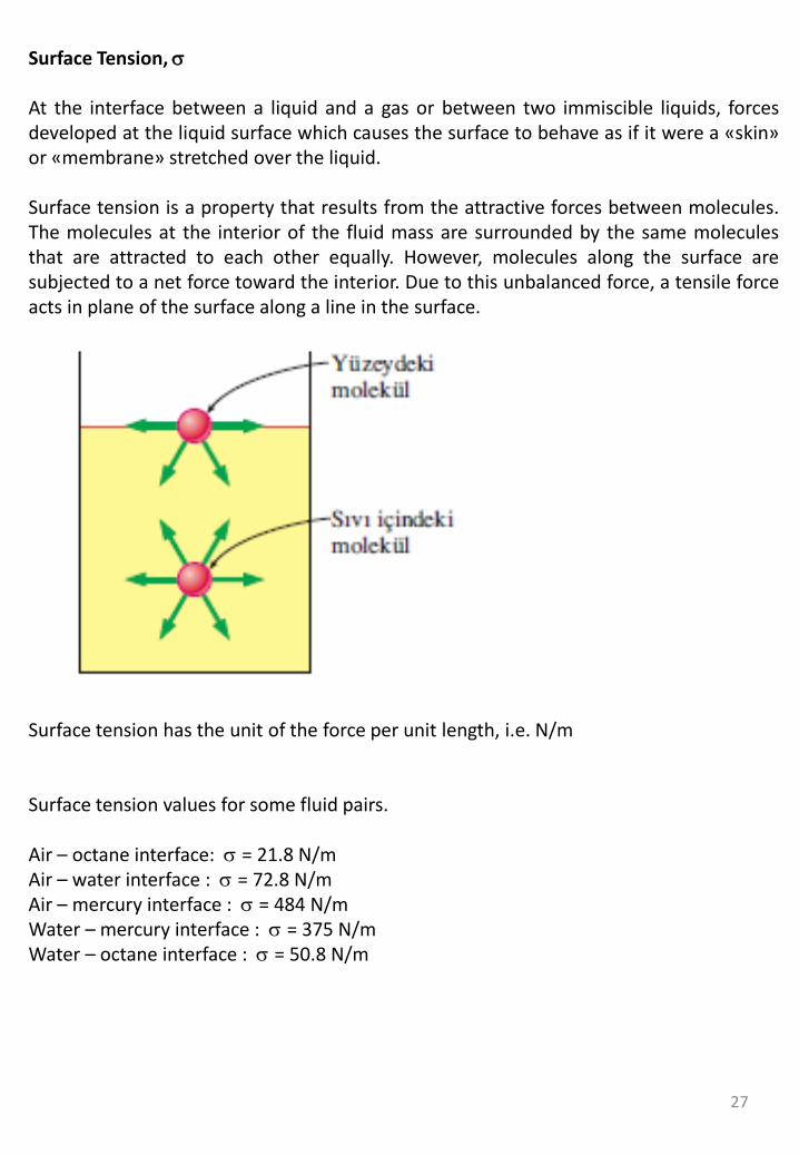
At the interface between a liquid and a gas or between two immiscible liquids, forcesdeveloped at the liquid surface which causes the surface to behave as if it were a «skin»or «membrane» stretched over the liquid.

Surface tension is a property that results from the attractive forces between molecules.The molecules at the interior of the fluid mass are surrounded by the same moleculesthat are attracted to each other equally. However, molecules along the surface aresubjected to a net force toward the interior. Due to this unbalanced force, a tensile forceacts in plane of the surface along a line in the surface.

Surface tension has the unit of the force per unit length, i.e. N/m

Surface tension values for some fluid pairs.

Air – octane interface: s = 21.8 N/mAir – water interface : s = 72.8 N/mAir – mercury interface : s = 484 N/mWater – mercury interface : s = 375 N/mWater – octane interface : s = 50.8 N/m

28

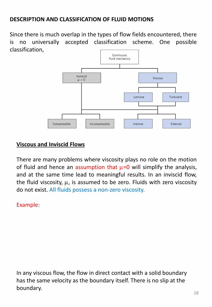
DESCRIPTION AND CLASSIFICATION OF FLUID MOTIONS

Since there is much overlap in the types of flow fields encountered, thereis no universally accepted classification scheme. One possibleclassification,

Viscous and Inviscid Flows

There are many problems where viscosity plays no role on the motionof fluid and hence an assumption that =0 will simplify the analysis,and at the same time lead to meaningful results. In an inviscid flow,the fluid viscosity, , is assumed to be zero. Fluids with zero viscositydo not exist. All fluids possess a non-zero viscosity.

Example:

In any viscous flow, the flow in direct contact with a solid boundary has the same velocity as the boundary itself. There is no slip at the boundary.

29

Laminar and Turbulent Flows

The laminar flow is characterized by smooth motion of fluid particles in laminae or layers.

The turbulent flow is characterized by random, three-dimensional motions of fluid particles superimposed on the mean motion.

In laminar flow there is no microscopic mixing of adjacent fluid layer.

Examples: