Lecture 9

Econ 2001

2015 August 20

Lecture 9 Outline

1 Linear Functions2 Linear Representation of Matrices3 Analytic Geometry in Rn : Lines and Hyperplanes4 Separating Hyperplane Theorems

Back to vector spaces so that we can illustrate the formal connection betweenlinear functions and matrices.

This matters for a lot calculus since derivatives are linear functions.

Then some useful geometry in Rn .

Announcements:- Test 2 will be tomorrow at 3pm, in WWPH 4716, and there will be recitation at1pm. The exam will last an hour.

Linear Transformations

DefinitionLet X and Y be two vector spaces. We say T : X → Y is a linear transformation if

T (α1x1 + α2x2) = α1T (x1) + α2T (x2) ∀x1, x2 ∈ X , α1, α2 ∈ RLet L(X ,Y ) denote the set of all linear transformations from X to Y .

L(X ,Y ) is a vector space.

ExampleThe function T : Rn −→ Rm defined by T (x) = Ax, with A

m×nis linear:

T (ax+ by) = A(ax+ by) = aAx+ bAy = aT (x) + bT (y)

Linear Functions

An equivalent characterization of linearityl : Rn −→ Rm is linear if and only if

1 for all x and y in Rn ,l(x+ y) = l(x) + l(y)

and2 for all scalars λ,

l(λx) = λl(x)

Linear functions are additive and exhibit constant returns to scale (econjargon).

If l is linear, then l(0) = 0 and, more generally, l(x) = −l(−x).

Compositions of Linear Transformations

The compositions of two linear functions is a linear functionGiven R ∈ L(X ,Y ) and S ∈ L(Y ,Z ), define S ◦ R : X → Z .

(S ◦ R)(αx1 + βx2) = S(R(αx1 + βx2))

= S(αR(x1) + βR(x2))

= αS(R(x1)) + βS(R(x2))

= α(S ◦ R)(x1) + β(S ◦ R)(x2)so S ◦ R ∈ L(X ,Z ).

Think about statement and proof for the equivalent characterization oflinearity.

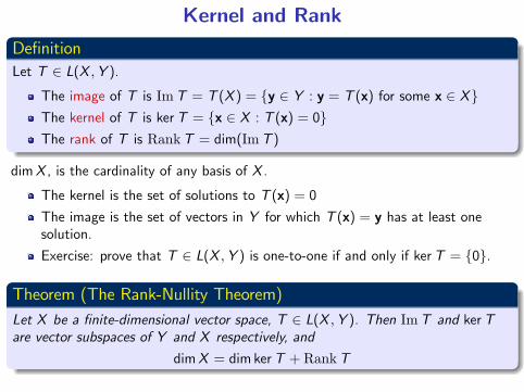
Kernel and RankDefinitionLet T ∈ L(X ,Y ).

The image of T is ImT = T (X ) = {y ∈ Y : y = T (x) for some x ∈ X}The kernel of T is kerT = {x ∈ X : T (x) = 0}The rank of T is RankT = dim(ImT )

dimX , is the cardinality of any basis of X .

The kernel is the set of solutions to T (x) = 0

The image is the set of vectors in Y for which T (x) = y has at least onesolution.

Exercise: prove that T ∈ L(X ,Y ) is one-to-one if and only if kerT = {0}.

Theorem (The Rank-Nullity Theorem)Let X be a finite-dimensional vector space, T ∈ L(X ,Y ). Then ImT and kerTare vector subspaces of Y and X respectively, and

dimX = dim kerT + RankT

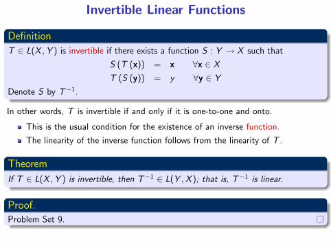
Invertible Linear Functions

DefinitionT ∈ L(X ,Y ) is invertible if there exists a function S : Y → X such that

S (T (x)) = x ∀x ∈ XT (S (y)) = y ∀y ∈ Y

Denote S by T−1.

In other words, T is invertible if and only if it is one-to-one and onto.

This is the usual condition for the existence of an inverse function.

The linearity of the inverse function follows from the linearity of T .

TheoremIf T ∈ L(X ,Y ) is invertible, then T−1 ∈ L(Y ,X ); that is, T−1 is linear.

Proof.Problem Set 9.

From Linear Functions to Matrices

l : Rn −→ Rm is linear if and only if (i) l(x+ y) = l(x) + l(y) andl(λx) = λl(x).

Any linear function is described by a matrix.

Compute l(ei ), where ei is the ith component of the standard basis in Rn .For each ei , l(ei ) is a vector in Rm , call it ai .Form A as the square matrix with ith column equal to ai .By construction, A has n columns and m rows and therefore f (x) = Ax for allx.

Next, apply this procedure to any linear basis of a vector space.

Using this observation, we derive a conection between composition of linearfunctions and multiplication of matrices.

Linear Transformations and Bases

If X and Y are vector spaces, to define a linear transformation T from X to Y , itis suffi cient to define T for every element of a basis for X .

Why?

Let V be a basis for X . Then every vector x ∈ X has a unique representationas a linear combination of a finite number of elements of V .

TheoremLet X and Y be two vector spaces, and let V = {vλ : λ ∈ Λ} be a basis for X .Then a linear function T ∈ L(X ,Y ) is completely determined by its values on V ,that is:

1 Given any set {yλ : λ ∈ Λ} ⊂ Y , ∃T ∈ L(X ,Y ) such that

T (vλ) = yλ ∀λ ∈ Λ

2 If S ,T ∈ L(X ,Y ) and S(vλ) = T (vλ) for all λ ∈ Λ, then S = T.

Linear Transformations and Bases

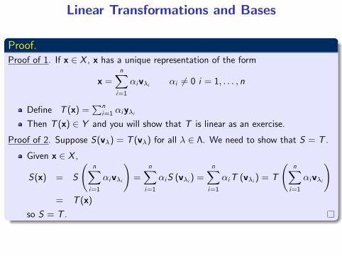
Proof.Proof of 1. If x ∈ X , x has a unique representation of the form

x =n∑i=1

αivλi αi 6= 0 i = 1, . . . , n

Define T (x) =∑n

i=1 αiyλiThen T (x) ∈ Y and you will show that T is linear as an exercise.

Proof of 2. Suppose S(vλ) = T (vλ) for all λ ∈ Λ. We need to show that S = T .

Given x ∈ X ,

S(x) = S

(n∑i=1

αivλi

)=

n∑i=1

αiS (vλi ) =n∑i=1

αiT (vλi ) = T

(n∑i=1

αivλi

)= T (x)

so S = T .

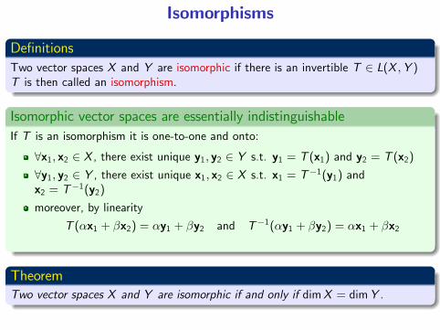
Isomorphisms

DefinitionsTwo vector spaces X and Y are isomorphic if there is an invertible T ∈ L(X ,Y )T is then called an isomorphism.

Isomorphic vector spaces are essentially indistinguishableIf T is an isomorphism it is one-to-one and onto:

∀x1, x2 ∈ X , there exist unique y1, y2 ∈ Y s.t. y1 = T (x1) and y2 = T (x2)∀y1, y2 ∈ Y , there exist unique x1, x2 ∈ X s.t. x1 = T−1(y1) andx2 = T−1(y2)moreover, by linearity

T (αx1 + βx2) = αy1 + βy2 and T−1(αy1 + βy2) = αx1 + βx2

TheoremTwo vector spaces X and Y are isomorphic if and only if dimX = dimY .

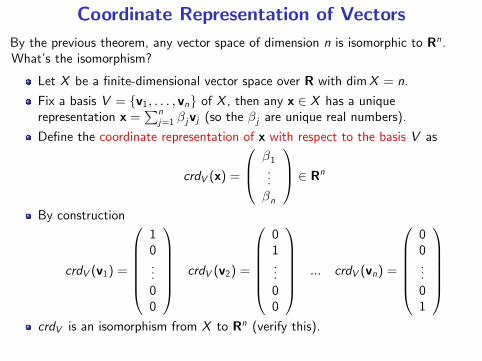
Coordinate Representation of VectorsBy the previous theorem, any vector space of dimension n is isomorphic to Rn .What’s the isomorphism?

Let X be a finite-dimensional vector space over R with dimX = n.

Fix a basis V = {v1, . . . , vn} of X , then any x ∈ X has a uniquerepresentation x =

∑nj=1 βjvj (so the βj are unique real numbers).

Define the coordinate representation of x with respect to the basis V as

crdV (x) =

β1...βn

∈ RnBy construction

crdV (v1) =

10...00

crdV (v2) =

01...00

... crdV (vn) =

00...01

crdV is an isomorphism from X to Rn (verify this).

Matrix Representation

Suppose T ∈ L(X ,Y ), where X and Y have dimension n and m respecively.

Fix bases V = {v1, . . . , vn} of X and W = {w1, . . . ,wm} of Y .

Since T (vj ) ∈ Y , we can write

T (vj ) =m∑i=1

αijwi

Define

MtxW ,V (T ) =

α11 · · · α1n...

. . ....

αm1 · · · αmn

Each column is given by crdW (T (vj )), the coordinates of T (vj ) with respect toW .

Thus any linear transformation from X to Y is equivalent to a matrix onceone fixes the two bases.

Matrix Representation

ExampleX = Y = R2, V = {(1, 0), (0, 1)}, W = {(1, 1), (−1, 1)};

Let T be the identity: T (x) = x for each x.

Notice that MtxW ,V (T ) 6=(1 00 1

). MtxW ,V (T ) is the matrix that

changes basis from V to W .

How do we compute it?

v1 = (1, 0) = α11(1, 1) + α21(−1, 1)α11 − α21 = 1 and α11 + α21 = 02α11 = 1, α11 = 1

2 hence α21 = − 12v2 = (0, 1) = α12(1, 1) + α22(−1, 1)

α12 − α22 = 0 and α12 + α22 = 12α12 = 1, α12 = 1

2 hence α22 = 12

So MtxW ,V (id) =

(1/2 1/2−1/2 1/2

)

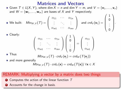
Matrices and VectorsGiven T ∈ L(X ,Y ), where dimX = n and dimY = m, and V = {v1, . . . , vn}and W = {w1, . . . ,wm} are bases of X and Y respectively.

We built: MtxW ,V (T ) =

α11 · · · α1n...

. . ....

αm1 · · · αmn

and crdV (v1) =

10...0

.Clearly: α11 · · · α1n

.... . .

...αm1 · · · αmn

10...0

=

α11...

αm1

Thus

MtxW ,V (T ) · crdV (vj ) = crdW (T (vj ))and more generally

MtxW ,V (T ) · crdV (x) = crdW (T (x)) ∀x ∈ X

REMARK: Multiplying a vector by a matrix does two things1 Computes the action of the linear function T2 Accounts for the change in basis.

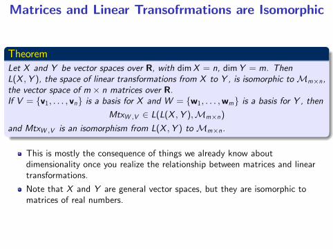
Matrices and Linear Transofrmations are Isomorphic

TheoremLet X and Y be vector spaces over R, with dimX = n, dimY = m. ThenL(X ,Y ), the space of linear transformations from X to Y , is isomorphic toMm×n ,the vector space of m × n matrices over R.If V = {v1, . . . , vn} is a basis for X and W = {w1, . . . ,wm} is a basis for Y , then

MtxW ,V ∈ L(L(X ,Y ),Mm×n)

and MtxW ,V is an isomorphism from L(X ,Y ) toMm×n .

This is mostly the consequence of things we already know aboutdimensionality once you realize the relationship between matrices and lineartransformations.

Note that X and Y are general vector spaces, but they are isomorphic tomatrices of real numbers.

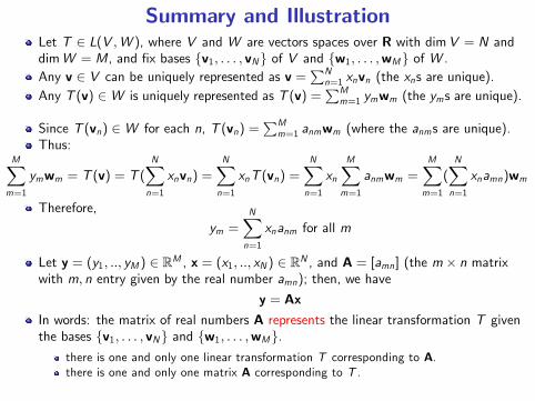
Summary and IllustrationLet T ∈ L(V ,W ), where V and W are vectors spaces over R with dimV = N anddimW = M, and fix bases {v1, . . . , vN} of V and {w1, . . . ,wM} of W .Any v ∈ V can be uniquely represented as v =

∑Nn=1 xnvn (the xns are unique).

Any T (v) ∈W is uniquely represented as T (v) =∑M

m=1 ymwm (the yms are unique).

Since T (vn) ∈W for each n, T (vn) =∑M

m=1 anmwm (where the anms are unique).Thus:

M∑m=1

ymwm = T (v) = T (N∑n=1

xnvn) =N∑n=1

xnT (vn) =N∑n=1

xnM∑m=1

anmwm =M∑m=1

(N∑n=1

xnamn)wm

Therefore,

ym =N∑n=1

xnanm for all m

Let y = (y1, .., yM ) ∈ RM , x = (x1, .., xN ) ∈ RN , and A = [amn] (the m × n matrixwith m, n entry given by the real number amn); then, we have

y = AxIn words: the matrix of real numbers A represents the linear transformation T giventhe bases {v1, . . . , vN} and {w1, . . . ,wM}.

there is one and only one linear transformation T corresponding to A.there is one and only one matrix A corresponding to T .

Matrix Product as Composite TransformationSuppose we have another linear transformation S ∈ L(W ,Q) where Q is a vectorspace with basis {q1, . . . ,qJ}.Let B = [bjm ] be the J ×M matrix representing S with respect to the bases{w1, . . . ,wM} and {q1, . . . ,qJ} for W and Q, respectively.Then, for all m, S(wm) =

∑Jj=1 bjmqj .

S ◦ T : V → Q is the linear transformation S ◦ T (v) = S(T (v)).Using the same logic of the previous slide:

S ◦ T (vn) = S(T (vn)) = S(M∑m=1

anmwm)

=M∑m=1

anmS(wm) =M∑m=1

anmJ∑j=1

bjmqj =J∑j=1

(M∑m=1

bjmamn)qj

ThereforeS ◦ T (vn) =

J∑j=1

cjnqj

wherecjn =

M∑m=1

bjmamn for j = 1, ..., J

Thus the J × N matrix C = [cjn] represents S ◦ T .What is C? The product BA (check the definition of matrix product).

Analytic Geomtetry: Lines

How do we talk about points, lines, planes,... in Rn?

DefinitionA line in Rn is described by a point x and a direction v . It can be represented as

{z ∈ Rn : there exists t ∈ R such that z = x+ tv}

If t ∈ [0, 1], this is the line segment connecting x to x+ v.

REMARKEven in Rn two points still determine a line: the line connecting x to y is the linecontaining x in the direction v.

Check that this is the same as the line through y in the direction v.

Analytic Geomtetry: Hyperplanes

DefinitionA hyperplane is a set described by a point x0 ∈ Rn and a normal direction of theplane p ∈ Rn , p 6= 0. It can be represented as

{z ∈ Rn : p · (z− x0) = 0}.

A hyperplane consists of all the z such that the direction z− x0 is orthogonalto p.Hyperplanes can equivalently be written as p · z = p · x0 (and if x0 = 0 this isp · z = 0)

In R2 lines are also hyperplanes. In R3 hyperplanes are “ordinary”planes.

REMARKLines and hyperplanes are two kinds of “flat” subsets of Rn .

Lines are subsets of dimension one.

Hyperplanes are subsets of dimension n − 1 or co-dimension one.One can have flat subsets of any dimension less than n.

Linear Manifolds

Lines and hyperplanes are not subspaces because they do not contain theorigin. (what is a subspace anyhow?)

They are obtained by “translating”a subspace: adding the same constant toall of its elements.

DefinitionA linear manifold of Rn is a set S such that there is a subspace V on Rn andx0 ∈ Rn with

S = V + {x0} ≡ {y : y = v + x0 for some v ∈ V }

Lines and hyperplanes are linear manifolds (not linear subspaces).

Lines

Here is another way to describe a line.

Given two points x and y in Rn , the line that passes through these points is:{z ∈ Rn : z = x+ t(y − x) for some t}.

This is called “parametric” representation (it defines n equations).

ExampleGiven y, x ∈ R2, we find a line through them by solving:

z1 = x1 + t(y1 − x1) and z2 = x2 + t(y2 − x2).Solve the first equation for t and substite out:

z2 = x2 +(y2 − x2) (z1 − x1)

y1 − x1or z2 − x2 =

y2 − x2y1 − x1

(z1 − x1) .

This is the standard way to represent the equation of a line (in the plane) through(x1, x2) with slope (y2 − x2)(y1 − x1).

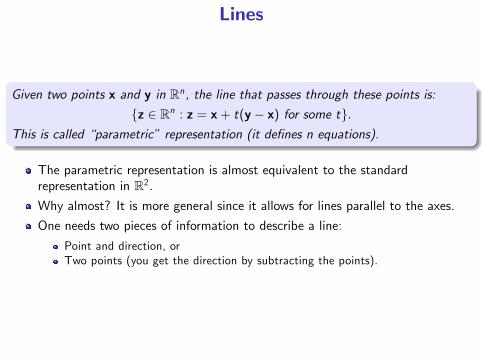
Lines

Given two points x and y in Rn , the line that passes through these points is:{z ∈ Rn : z = x+ t(y − x) for some t}.

This is called “parametric” representation (it defines n equations).

The parametric representation is almost equivalent to the standardrepresentation in R2.Why almost? It is more general since it allows for lines parallel to the axes.

One needs two pieces of information to describe a line:

Point and direction, orTwo points (you get the direction by subtracting the points).

Hyperplanes

How does one describe an hyperplane?

One way is to use a point and a (normal) direction

{z ∈ Rn : p · (z− x0) = 0}

Another way is to use n points in Rn , provided these are in “general position.”You can go from points to the normal solving a linear system of equations.

How to Find an Hyperplane when n=3

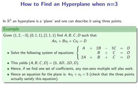
In R3 an hyperplane is a ‘plane’and one can describe it using three points.

ExampleGiven (1, 2,−3), (0, 1, 1), (2, 1, 1) find A,B,C ,D such that

Ax1 + Bx2 + Cx3 = D

Solve the following system of equations:

A + 2B − 3C = DB + C = D

2A + B + C = D

This yields (A,B,C ,D) = (0, .8D, .2D,D).

Hence, if we find one set of coeffi cients, any non-zero multiple will also work.

Hence an equation for the plane is: 4x2 + x3 = 5 (check that the three pointsactually satisfy this equation).

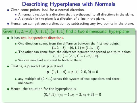
Describing Hyperplanes with NormalsGiven some points, look for a normal direction.

A normal direction is a direction that is orthogonal to all directions in the plane.A direction in the plane is a direction of a line in the plane.

Hence, we can get such a direction by subtracting any two points in the plane.

Given (1, 2,−3), (0, 1, 1), (2, 1, 1) find a two dimensional hyperplaneIt has two independent directions.

One direction comes from the difference between the first two points:(1, 2,−3)− (0, 1, 1) = (1, 1,−4).

The other can come from the difference between the second and third points(0, 1, 1)− (2, 1, 1) = (−2, 0, 0).

We can now find a normal to both of them.

That is, a p such that p 6= 0 and

p · (1, 1,−4) = p · (−2, 0, 0) = 0

any multiple of (0, 4, 1) solves this system of two equations and threeunknowns.

Hence, the equation for the hyperplane is

(0, 4, 1) · (x1 − 1, x2 − 2, x3 + 3) = 0

Separating Hyperplanes and Convexity

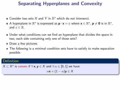
Consider two sets X and Y in Rn which do not interserct.A hyperplane in Rn is expressed as p · x = c where x ∈ Rn , p 6= 0 is in Rn ,and c ∈ R.

Under what conditions can we find an hyperplane that divides the space intwo, each side containing only one of those sets?

Draw a few pictures.

The following is a minimal condition sets have to satisfy to make separationpossible.

DefinitionX ⊂ Rn is convex if ∀ x, y ∈ X and ∀α ∈ [0, 1] we have

αx+ (1− α)y ∈ X

Separating Hyperplane Theorem

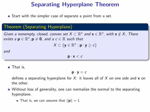
Start with the simpler case of separate a point from a set.

Theorem (Separating Hyperplane)Given a nonempty, closed, convex set X ⊂ Rn and x ∈ Rn , with x /∈ X, Thereexists a p ∈ Rn ,p 6= 0, and a c ∈ R such that

X ⊂ {y ∈ Rn : p · y ≥ c}and

p · x < c

That is,p · y = c

defines a separating hyperplane for X : it leaves all of X on one side and x onthe other.

Without loss of generality, one can normalize the normal to the separatinghyperplane.

That is, we can assume that ‖p‖ = 1.

Proof of the separating hyperplane theorem in 9(+1 for you) stepsConsider the problem of minimizing the distance between x and X . That is: find avector that solves miny∈X ‖x− y‖.

1 X is nonempty, so we can find some element z ∈ X . While X is notnecessarily bounded, without loss of generality we can replace X by{y ∈ X : ‖y − x‖ ≤ ‖z− x‖}. This set is compact because X is closed.

2 The norm is a continuous function. Hence there is a solution y∗.3 Let p = y∗ − x. Since x /∈ X , p 6= 0.4 Let c = p · y∗. Since c − p · x = p · (y∗ − x) = ‖p‖2, therefore c > p · x.5 We need to show if y ∈ X , then p · y ≥ c .6 Notice how this inequality is equivalent to

(y∗ − x) · (y − y∗) ≥ 0.7 Since X is convex and y∗ solves the minimzation problem, it must be that

‖ty + (1− t)y∗ − x‖2

is minimized when t = 0.8 Since the derivative of ‖ty + (1− t)y∗ − x‖2 is non-negative at t = 0, thefirst order condition will do it.

9 Check that differentiating ‖ty + (1− t)y∗ − x‖2 (as a function of t) andsimplifying yields the desired inequality.

Extensions

If x is in the boundary of X , then you can approximate x by a sequence xksuch that each xk /∈ X .

This yields a sequence of pk , which can be taken to be unit vectors, that satisfythe conclusion of the theorem.A subsequence of the pk must converge.The limit point p∗ will satisfy the conclusion of the theorem (except we canonly guarantee that c ≥ p∗ · x rather than the strict equality).

The closure of any convex set is convex.

Given a convex set X and a point x not in the interior of the set, we canseparate x from the closure of X .

Putting these things together...

A Stronger Separating Hyperplane TheoremTheorem (Supporting Hyperplane)Given a convex set X ⊂ Rn and x ∈ Rn , x. If x is not in the interior of X , thenthere exists p ∈ Rn ,p 6= 0, and c ∈ R such that

X ⊂ {y ∈ Rn | p · y ≥ c}and

p · x ≤ c

Other general versions separate two convex sets. The easiest case is when thesets do not have any point in common, and the slightly harder is the one inwhich no point of one set is in the interior of the other set.

Let A,B ⊆ Rn be nonempty, disjoint convex sets. Then there exists a nonzerovector p ∈ Rn such that

p · a ≤ p · b ∀a ∈ A, b ∈ B

The separating hyperplane theorem can be used to provide intuition for theway we solve constrained optimization problems.In the typical economic application, the separating hyperplane’s normal is aprice vector, and the separation property states that a particular vector costsmore than vectors in a consumption set.

Tomorrow

Calculus

1 Level Sets2 Derivatives and Partial Derivatives3 Differentiability4 Tangents to Level Sets