ORNL/TM-2014/144

LCCP Desktop Application v1.0 Engineering Reference

October 31, 2013

Prepared by Mohamed Beshr Vikrant C. Aute

Approved for public release: distribution is unlimited.

DOCUMENT AVAILABILITY

Reports produced after January 1, 1996, are generally available free via the U.S. Department of Energy (DOE) Information Bridge. Web site http://www.osti.gov/bridge Reports produced before January 1, 1996, may be purchased by members of the public from the following source. National Technical Information Service 5285 Port Royal Road Springfield, VA 22161 Telephone 703-605-6000 (1-800-553-6847) TDD 703-487-4639 Fax 703-605-6900 E-mail info@ntis.gov Web site http://www.ntis.gov/support/ordernowabout.htm Reports are available to DOE employees, DOE contractors, Energy Technology Data Exchange (ETDE) representatives, and International Nuclear Information System (INIS) representatives from the following source. Office of Scientific and Technical Information P.O. Box 62 Oak Ridge, TN 37831 Telephone 865-576-8401 Fax 865-576-5728 E-mail reports@osti.gov Web site http://www.osti.gov/contact.html

This report was prepared as an account of work sponsored by an agency of the United States Government. Neither the United States Government nor any agency thereof, nor any of their employees, makes any warranty, express or implied, or assumes any legal liability or responsibility for the accuracy, completeness, or usefulness of any information, apparatus, product, or process disclosed, or represents that its use would not infringe privately owned rights. Reference herein to any specific commercial product, process, or service by trade name, trademark, manufacturer, or otherwise, does not necessarily constitute or imply its endorsement, recommendation, or favoring by the United States Government or any agency thereof. The views and opinions of authors expressed herein do not necessarily state or reflect those of the United States Government or any agency thereof.

1

Table of Contents

1. Introduction .......................................................................................................................... 3

Part 1: Objectives, Literature Review and Mathematical Background .......................................... 4

2. Overall Life Cycle Climate Performance Objective ............................................................ 4

3. Literature Review................................................................................................................. 4

4. Mathematical Background ................................................................................................... 5

4.1. Direct Emissions ........................................................................................................... 5

4.1.1. Emissions due to refrigerant leakage .................................................................... 5

4.1.2. Irregular emissions due to such things as accidents .............................................. 6

4.1.3. Emissions due to leakage of refrigerant during servicing ..................................... 6

4.1.4. Emissions due to system end-of-life refrigerant loss ............................................ 6

4.1.5. Emissions due to leakage from the refrigerant production and transportation ..... 7

4.1.6. Direct emissions .................................................................................................... 7

4.2. Indirect Emissions ........................................................................................................ 7

4.2.1. Emission due to energy used to manufacture components of system ................... 7

4.2.2. Emission due to energy used to manufacture refrigerant ...................................... 8

4.2.3. Emission due to energy used to recycle end-of-life of components ..................... 8

4.2.4. Emission due to energy used for end-of-life of refrigerants ................................ 9

4.2.5. Emission due to energy used to transport equipment ........................................... 9

4.2.6. Emission due to energy consumption of system during system’s lifetime ........... 9

4.2.7. Indirect emissions ................................................................................................ 10

4.3. Total Emissions .......................................................................................................... 10

Part 2: Input Data ......................................................................................................................... 11

5. Application Information ..................................................................................................... 11

2

5.1. Select a Location ........................................................................................................ 11

6. Load Information ............................................................................................................... 11

6.1. Load Type ................................................................................................................... 12

6.1.1. Built-In ................................................................................................................ 12

6.1.2. File based ............................................................................................................. 12

6.1.3. EnergyPlus .......................................................................................................... 12

6.1.4. AHRI Standard .................................................................................................... 12

7. Simulation Information ...................................................................................................... 13

7.1. Centralized DX or Secondary Loop Systems ............................................................. 13

7.1.1. Path to executable ................................................................................................ 13

7.1.2. Template file ....................................................................................................... 13

7.1.3. Working folder path ............................................................................................ 14

7.1.4. Command ............................................................................................................ 14

7.1.5. Account for charge degradation .......................................................................... 14

7.2. Air Source Heat Pump (ASHP) System ..................................................................... 17

7.3. Display Cases Using Secondary Refrigerants ............................................................ 17

7.4. Water Chiller .............................................................................................................. 17

8. LCCP Tool Flow Charts .................................................................................................... 18

9. VapCyc Executable ............................................................................................................ 21

10. EnergyPlus ..................................................................................................................... 22

Part 3: Interfaces .......................................................................................................................... 25

11. LCCP interfaces ............................................................................................................. 25

References ..................................................................................................................................... 29

3

LCCP Desktop Application v1.0 Engineering Reference

1. Introduction

This Life Cycle Climate Performance (LCCP) Desktop Application Engineering Reference is

divided into three parts. The first part of the guide, consisting of the LCCP objective, literature

review, and mathematical background, is presented in Sections 2-4. The second part of the guide

(given in Sections 5-10) provides a description of the input data required by the LCCP desktop

application, including each of the input pages (Application Information, Load Information, and

Simulation Information) and details for interfacing the LCCP Desktop Application with the

VapCyc and EnergyPlus simulation programs. The third part of the guide (given in Section 11)

describes the various interfaces of the LCCP code.

Figure 1 shows the main ORNL LCCP framework. The LCCP calculation methodology

represents the core of the software. However, three main categories of inputs are required for

these calculations. These categories are the emission and weather data (obtained from databases

such as the TMY3 weather data), the load model (obtained from EnergyPlus, TRNSYS…etc.),

and the system model (obtained from system performance models, or performance maps based

on catalog data or experiments).

Figure 1: ORNL LCCP Framework.

4

Part 1: Objectives, Literature Review and Mathematical

Background

2. Overall Life Cycle Climate Performance Objective

The objective of Life Cycle Climate Performance (LCCP) analysis is to evaluate the equivalent

mass of carbon dioxide released into the atmosphere due to a refrigeration system’s performance,

throughout its lifetime, from system construction through system operation and system

destruction. The carbon dioxide emissions from a refrigeration system can be divided into two

broad categories: direct emissions and indirect emissions. Direct emissions include the

environmental impact of leakage of refrigerant which occurs during system operation. Indirect

emissions include the environmental impact associated with the production and distribution of

the energy required to operate the refrigeration system.

3. Literature Review

Sand et al. (1997) looked at the Total Equivalent Warming Impact (TEWI) of alternative

refrigerants. They found insignificant decrease in TEWI in the use of ammonia and hydrocarbons

as refrigerants for refrigeration systems with low emissions.

Papasavva et al. (2010) explained the workings of the GREEN-MACLCCP model in “GREEN-

MAC-LCCP: A Tool for Assessing the Life Cycle Climate Performance of Mobile Air

Conditioning (MAC) Systems.” In this paper they describe the methodology of the model as well

as sample results generated from the model.

Deru and Torcellini (2007) detail the emission associated with energy usage in “Source Energy

and Emission Factors for Energy Use in Buildings.” In this report they detail the breakdown of

the electricity grid in the United States as well as report the equivalent carbon dioxide emissions

for electricity consumption in the different regions of the United States.

Hwang et al. (2007) experimentally tested walk-in refrigeration systems that simulate direct

expansion commercial refrigeration systems with small charge utilizing R404A, R-410A, and R-

290 as refrigerants. They found that the LCCP of R-290A is always lower than that of R-404A.

5

TMY3 data from the National Solar Radiation Data Base (NREL 2012a) details weather data for

a number of different cities throughout the United States, including cities in such varied locations

as Phoenix, Arizona, Los Angles, California, Chicago, Illinois, and New York, New York. The

data sets include dry-bulb temperature (DBT), dew-point temperature, and relative humidity

(RH) for all 8760 hours of the year.

The National Renewable Energy Laboratory maintains a Life Cycle Inventory database (NREL

2012b). Its goals include maintaining an accounting database that provides cradle-to-grave

information about energy flows.

4. Mathematical Background

The following section provides the detailed mathematical procedure that is used in the LCCP

Desktop Application for determining the carbon dioxide equivalent emissions of a system over

its lifetime. The total emissions of a system are composed of direct emissions (due to direct

leakage of refrigerant which occurs during system operation) and indirect emissions (due to the

production and distribution of the energy associated with the construction, operation and

decommissioning of the refrigeration system).

4.1.Direct Emissions

Papasavva et al. (2010) separate direct emissions into six categories, which are discussed below.

4.1.1. Emissions due to refrigerant leakage

Refrigeration systems oftentimes leak refrigerant during system operation. The direct emissions

resulting from refrigerant leakage can be calculated as follows:

Emissions due to = System Charge * System Lifetime * Annual Leakage Rate *

refrigerant leakage Global Warming Potential (GWP) of Refrigerant (1)

where System Charge (lb), System Lifetime (years), and Annual Leakage Rate (as a percentage of

system the charge) are input by the user.

6

4.1.2. Irregular emissions due to such things as accidents

Irregular emissions of refrigerant from the refrigeration system are due to unforeseen incidents

and accidents. The direct emissions due to these accidents can be calculated as follows:

Emissions due to accidents = System Charge * System Lifetime * Annual Accident

Emission Rate * GWP of Refrigerant (2)

where System Charge (lb), System Lifetime (years), and Annual Accident Emission Rate (as a

percentage of the system charge) are input by the user. If the user does not input a value for the

Annual Accident Emission Rate, then the default value of zero will be used.

4.1.3. Emissions due to leakage of refrigerant during servicing

During refrigeration system servicing events, refrigerant may leak from the system. The direct

emissions due to leakage of refrigerant resulting from servicing events can be calculated as

follows:

Emissions due to servicing = Number of services in lifetime * System Charge

* Servicing Leakage Rate * GWP of Refrigerant (3)

where

Number of services in lifetime = System Lifetime / Service Interval;

and the System Charge (lb), System Lifetime (years), Service Interval, and Servicing Leakage

Rate (as a percentage of the system charge) are input by the user. If the user does not input a

value for the Servicing Leakage Rate, then the default value of zero will be used.

4.1.4. Emissions due to system end-of-life refrigerant loss

At the end of the useful life of the refrigeration system, the refrigerant in the system will be

recovered prior to disassembly. During the refrigerant recovery process, a small quantity of

refrigerant is inevitably released into the atmosphere. The direct emissions associated with the

end-of-life loss of refrigerant can be calculated as follows:

Emissions due to end-of-life of system = Percentage of Refrigerant Lost at End-of-Life *

System Charge * GWP of Refrigerant (4)

7

where the System Charge (lb), and the Percentage of Refrigerant Lost at End-of-Life are input by

the user.

4.1.5. Emissions due to leakage from the refrigerant production and transportation

When refrigerant is produced and transported to the location where it will be utilized, refrigerant

leakage will occur. The direct emissions associated with refrigerant production and

transportation losses can be calculated as follows:

Emissions due to production = System Charge * Refrigerant Production and Transportation

and transportation Leakage Rate * GWP of Refrigerant (5)

where the System Charge (lb) and the Refrigerant Production and Transportation Leakage Rate

(as a percentage of the system charge) are input by the user. If the user does not input a value for

the Refrigerant Production and Transportation Leakage Rate, then the default value of zero will

be used.

4.1.6. Direct emissions

The aforementioned six contributors to the direct emissions may be combined to yield the total

direct emissions as follows:

Direct Emissions = Emissions due to refrigerant leakage + Irregular emissions due to such

things as accidents + Emissions due to leakage of refrigerant from

servicing + Emissions due to end-of-life of system where refrigerant is lost

+ Emissions due to leakage that occurs from the refrigerant production and

transportation + Reaction byproducts that occur from the atmospheric

breakdown of the refrigerant emissions (6)

4.2.Indirect Emissions

Papasavva et al. (2010) divide indirect emissions into six categories, which are discussed below.

4.2.1. Emission due to energy used to manufacture components of system

The indirect emissions associated with the energy that is used to manufacture the components of

the refrigeration system is calculated as follows:

8

Emission due to energy used to manufacture = Mass of each material *

components of system CO2 equivalent (7)

The CO2 equivalent term for each material is obtained from a database contained within the

LCCP Desktop Application. The mass and material type of each component is specified by the

user.

4.2.2. Emission due to energy used to manufacture refrigerant

The indirect emissions associated with the energy used to make the refrigerant itself is calculated

as follows:

Emission due to energy used to = System Charge * (1 + System Lifetime * Annual Leak

manufacture refrigerant Rate – Percentage of reused refrigerant) * CO2

equivalent emissions for virgin refrigerant (8)

Equation (8) accounts for the refrigerant manufacturing emissions for the virgin refrigerant for

all of the system charge, including the charge in the system and the charge leaked out of the

system during the system’s lifetime. The CO2 equivalent emissions for virgin refrigerant is

obtained from a database contained within the LCCP Desktop Application.

4.2.3. Emission due to energy used to recycle end-of-life of components

The indirect emissions associated with the energy used to recycle the metal and plastic

components of the refrigeration system at the end of the system’s useful life is calculated as

follows:

Emission due to energy used for = Energy of Recycling of metals * mass of metals * CO2

end-of-life components equivalent of metals + Energy of Recycling of Plastics *

mass of plastics* CO2 equivalent of plastics (9)

In equation (9), the energy required to recycle metals and plastics, and the carbon dioxide

equivalent of metals and plastics is obtained from Papasavva et al. (2010). The masses of metals

and plastics will be obtained from the refrigeration systems themselves, as specified by the user.

9

4.2.4. Emission due to energy used for end-of-life of refrigerants

This factor quantifies the indirect emissions associated with the energy used to dispose of or

recycle the refrigerants at the end of the useful life of the refrigeration system. The user enters a

value for the total (throughout the life of the system) emissions due to refrigerant disposal or

recycling (in kgCO2eq) as he or she sees fit. If the user does not enter a value for this factor, the

default value of zero will be used.

4.2.5. Emission due to energy used to transport equipment

This factor quantifies the indirect emissions associated with the energy used to transport the

refrigeration system from the manufacturing plant to the store location. The user enters a value

for the total (throughout the life of the system) emissions due to energy used to transport the

equipment (in kgCO2eq) as he or she sees fit. If the user does not enter a value for this factor, the

default value of zero will be used.

4.2.6. Emission due to energy consumption of system during system’s lifetime

This factor, which is probably the single biggest contributor to total emissions, involves the

carbon dioxide equivalent emissions at the power plant related to the production and distribution

of electrical energy that the refrigeration system utilizes. The indirect emissions associated with

the energy consumption of the refrigeration system is calculated as follows:

Emission due to energy consumption = System Lifetime * Annual Energy Consumed *

of system during system’s lifetime Average Emission Rate for Specified Location (10)

The Average Emission Rate for Specified Location is obtained from Deru and Torcellini (2007).

To calculate the annual energy usage of the system, the following process will be used:

1) The ambient temperatures for all 8760 hours of a year will be obtained from Typical

Meteorological Year (TMY) data. The TMY3 data will be obtained from the National

Solar Radiation Database (NREL 2012a). In addition to taking temperature from all 8760

hours, binned data will be used to increase the speed of calculations.

2) These hourly ambient temperatures will then be used by VapCyc (or any other system

simulation software) as the hourly environmental temperatures that the condenser is

subjected to.

10

3) The power output from VapCyc is the power consumed by the compressor. Summing the

power over all 8760 hours in a year, or summing the binned power data, yields the

Annual Energy Consumed, as used in Equation (11) above.

4.2.7. Indirect emissions

The aforementioned six contributors to the indirect emissions may be combined to yield the total

indirect emissions as follows:

Indirect Emissions = Emission due to energy used to manufacture components of system

+ Emission due to energy used to manufacture refrigerant +

Emission due to energy used for end of-life of components +

Emission due to energy used for end-of-life of refrigerants +

Emission due to energy consumption of system during system’s

lifetime + Emission due to energy used to transport equipment (11)

4.3.Total Emissions

Finally, the total emission, which is the ultimate objective of the LCCP analysis and includes the

contributions from direct and indirect sources, is given by:

Total Emissions = Direct Emissions + Indirect Emissions (12)

11

Part 2: Input Data

The input data required by the LCCP Desktop Application is entered in three main pages:

Application Information, Load Information, and Simulation Information. A description of each

of these input pages in addition to details for interfacing the LCCP Desktop Application with the

VapCyc and EnergyPlus simulation programs is given in the following sections.

5. Application Information

This part of the inputs contains the input data which are used for the LCCP calculations (i.e.

direct and indirect emissions). The different refrigerant leakage rates are input by the user and

are used by the LCCP core to calculate the direct emissions and the indirect emissions except the

indirect emissions due to the system’s power consumption. The indirect emissions due to the

system’s power consumption are calculated based on the “Load Inputs” and “Simulation Inputs”

for the code as explained in section 9, or based only on the “Load Inputs” as explained in section

10.

Also, this section contains the required information to obtain the hourly DBT, and RH. These

values will be used together with the “Load Inputs” to create an input text file which will be

placed in the working folder path (see section 7.3) for use by the system simulation software to

calculate the system’s hourly power consumption.

5.1.Select a Location

The user selects the location for which the LCCP calculations will be performed (i.e. the city

where the analyzed system will be operated). Based on the location, the weather data, and the

emissions values will be obtained from the TMY3 data files. The TMY3 files are found in the

“AppFolder” folder in the installation directory of the LCCP desktop software. The

“TMY3DataFiles” folder contains the weather data files while the “TMY3EmissionDataFiles”

folder contains the emissions data. The files inside each folder follow the TMY3 nomenclature.

6. Load Information

The Load Information page contains the information required to specify the hourly absolute load

values. These load values are used to create an input text file which is placed in the working

12

folder path and provided to the system simulation software to calculate the system’s hourly

power consumption. Also, the system’s hourly power consumption can be specified directly, as

explained in section 10.

6.1.Load Type

The user can select from three different load calculation methods:

6.1.1. Built-In

This option allows the user to specify the hourly load based on the nominal value (input by the

user in the Application Information page), and a predefined hourly load profile (containing

percentages of the nominal load).

6.1.2. File based

This option allows the hourly load to be specified via a user-supplied text file. The input file

should be in a comma separated value format (.csv) with the load values being in the second

column (and the first column can be the hour). This file can either contain the absolute load

values in Watts (W) for every hour of the year or hourly values for the load as a percentage of

the nominal load. Also, the file can contain the absolute power consumption values in Watt-hr

(W-hr) for every hour of the year.

6.1.3. EnergyPlus

This option allows for the specification of the hourly load values through the use of a load

calculation software (e.g. EnergyPlus). For this method, the user specifies the paths to the files

required to run the load calculation software (see section 10 for more details). When the user

selects this method, the option to either use EnergyPlus to obtain the hourly load values (and

then run a system simulation software such as VapCyc) or directly obtain the system’s hourly

power consumption from EnergyPlus (without running a system simulation software) can be

selected.

6.1.4. AHRI Standard

This option is only available when an air source heat pump (ASHP) system is selected. This

option calculates the hourly load according to ANSI/AHRI Standard 210/240 (2008). Equations

13

4.1-2 and 4.2-2 in the standard are used for the calculation of the cooling load, and heating load,

respectively.

7. Simulation Information

In the Simulation Information page, the user specifies the data related to the system simulation.

These data together with the load and weather data (specified in the Application Information

page) are used to calculate the system’s hourly and total annual power consumption. This part is

required for the LCCP calculations unless the load type is file based (section 6.1.2) with absolute

power consumption, or the calculation software (e.g. EnergyPlus) is used to directly obtain the

system’s hourly power consumption as explained in section 10.

7.1.Centralized DX or Secondary Loop Systems

For these two system types, a system simulation software is used to determine the hourly power

consumption. The required inputs are explained in the following sections.

7.1.1. Path to executable

The user browses and selects the system simulation software (e.g. VapCyc) executable. This

executable is supplied by the user and returns the “capacity” and “power consumption” of the

system for every hour of the year (i.e. 8760 values of the system’s capacity and power

consumption). The output file should be in either a tab separated values format or a comma

separated values (csv) format.

7.1.2. Template file

The user browses and selects the system simulation software input file template. This is simply

the input file which will be read by the system simulation software in order to determine the

capacity and power consumption. A sample template file for the VapCyc software is found in the

“samples” folder in the “workingdirectory” folder located in the LCCP installation directory.

The template file can be modified by the user through the LCCP Simulation Information page. In

order to do this, the user can replace any line in the template file (the line with the desired value

change) with “Delimiter” + “Key” + “Delimiter” where “Delimiter” could be any symbol and

“Key” could be any string. The user then writes a friendly name (any name or note for this

parameter) in the LCCP user interface under the “Friendly Name” column. Also, the user writes

14

the key (i.e. “Key”) of the parameter in the “Key” column. Then, the user specifies the type of

the parameter being changed under the “Type” column and its new or desired value under the

“Value” column.

An example for this, based on the sample VapCyc template file, is replacing the condenser tube

length with any desired value through the LCCP user interface. Also, the “Delimiter” is “%%”

while the “Key” is “COND_TUBE_LENGTH”. First, the condenser tube length line in the

VapCyc file is replaced with the delimiter-key-delimiter string “%%COND_TUBE_LENGTH

%%” in order to create the VapCyc template file. Then, the key and the desired value are entered

in the LCCP inputs page. When the user runs the LCCP software, the program searches for the

“Key” in the template file and replaces it with the “value” specified by the user.

7.1.3. Working folder path

The user enters the path where the intermediate files will be saved. That is, this folder will have

an input file which is passed from the LCCP core to the simulation software executable and

contains the hourly weather data (DBT, and RH). The simulation software input file is simply the

template file which results after replacing the key lines with the desired values. Finally, this

folder will contain the output file written by the simulation software executable which will then

be read by the LCCP core to perform the LCCP calculations.

7.1.4. Command

The user enters the command which contains the simulation software executable name and input

arguments. For the VapCyc executable, this line has four inputs separated by a space. The first

one is the name of the executable file (e.g. Executable.exe). The second term is the load file

which is the input file to the system simulation tool and contains the hourly load and weather

data. The third one is the template file which the system simulation software will run. The last

term is the output file which is written by the executable and contains the system’s hourly

capacity and power consumption.

7.1.5. Account for charge degradation

The user can choose to account for the charge degradation on the system by checking the

“Account for Charge Degradation”. That is, the effect of refrigerant leak from the system,

causing it to be undercharged, between two consecutive services on the performance of the

15

system. When the user checks the “Account for Charge Degradation”, a new window pops up.

The user needs to enter the annual refrigerant slow leak rate, the charge limit after which the

charge degradation would start to affect the system performance, the indoor DBT if it is required

for the capacity and power consumption equations. In addition, the user needs to select the

correlations for the effect of the charge degradation on the system’s capacity and power

consumption.

When running the cycle, the solver runs the system simulation tool just once and then performs

the charge degradation calculations on the outputs. The charge decreases by an amount equal to

the annual refrigerant slow leakage rate based on the nominal charge for every year (e.g. if

charge is 100 lb and leakage rate is 5%, then after the first year the charge is 95, and after the

second year it is 90%, and so on) until servicing is performed. This is repeated for the lifetime of

the system.

A summary of some of the experimental studies done on the charge degradation effect on the

system performance is summarized in Table 1.

Table 1: Summary of studies on effect of system undercharging.

Study Year System

The Trane company 1976 Eight year old residential air conditioner

A. A. Domingorena 1980 3-ton air-to-air heat pump, R-22 refrigerant, heating mode

Houcek and Thedford

for Texas Power and

Light (TP&L)

1984 1.5 ton split system unit

Mohsen Farzad and

Dennis L. O'Neal

1988 3-ton Trane air conditioner with capillary tube expansion

Mohsen Farzad 1990 3-ton Trane air conditioner with three expansion devices

16

Robinson 1993 3-ton split-system heat pump operating in the cooling mode.

The heat pump had a scroll compressor and utilized an orifice

for the expansion device.

Angel Gerardo

Rodriguez

1995 Two air conditioning units were used. One was a three ton,

split-system air conditioner with a scroll compressor and a

short tube orifice as the expansion device. The other unit tested

was a 3.5 ton, split system air conditioner with a scroll

compressor and a thermostatic expansion valve.

D.Y. Goswami, G. Ek,

M. Leung,C.K. Jotshi

and S.A. Sherif

1997 R-22 3-ton residential air-conditioning system

J.M. Choi, Y.C. Kim 2001 Water-to-water heat pump. The nominal cooling capacity of the

tested heat pump was 3.5 kW, and the working fluid was R22

I.N. Grace, D. Datta,

S.A. Tassou

2005 A small 4 kW nominal cooling capacity vapor compression

water-to-water chiller equipped with plate type heat exchangers

Erin Kruse and Larry

Palmiter

2006 The heat pump tested was a 3-ton economy model with a rated

Seasonal Energy Efficiency Ratio (SEER) of 10 and a Heating

Seasonal Performance Factor (HSPF) of 7.2 (a 3-ton Carrier

YKC heat pump (R-22 refrigerant, suction-line accumulator) in

heating mode only). All of the measurements were performed

once with each of two metering devices: a short-tube orifice

(STO) and a thermostatic expansion valve (TXV) on the

outdoor unit.

Adam Wichman,

James E. Braun

2008 The cooler system utilized R-22 as the refrigerant, whereas the

freezer unit employed R-404A. Both systems were equipped

with a TXV expansion valve and a liquid line receiver.

17

Woohyun Kim, James

E. Braun

2010 see tables 1-4 in the paper

Bo Shen, James E.

Braun, Eckhard A.

Groll

2011 3-ton R-22 split heat pump in heating mode

7.2.Air Source Heat Pump (ASHP) System

The hourly power consumption of the system is calculated according to the procedure presented

in section 4 of the ANSI/AHRI Standard 210/240 (2008). The load type for an ASHP system is

either EnergyPlus or AHRI standard.

7.3.Display Cases Using Secondary Refrigerants

The hourly power consumption of the system is calculated according to the procedure presented

in section 5.2 of the ANSI/AHRI Standard 1320 (2011). There is no load input required for this

system.

7.4.Water Chiller

The hourly power consumption of the system is calculated using the ANSI/AHRI Standard

550/590 (2011) according to the following procedure:

1) The user enters some information about the performance at the part load rating conditions

specified in table 3 in the standard. That is, the user will enter the full capacity of the

system and the EER at 25%, 50%, and 75% load.

2) Based on this information and the hourly load profile, the hourly part load factor will be

determined. Thus, the hourly EER will be calculated using linear interpolation between

each of the user entered values (points). Thus, the hourly power consumption can be

calculated. If the user doesn’t have the data at the main part load factors (25%, 50%,

75%), the user can enter the data available and also linear interpolation will be applied

between each of the entered points (refer to section 5.4.1.2 in the standard). However, up

to this point the ambient temperature effect is not accounted for.

18

3) The user would enter 2 more inputs. The first one is an equation for the EER as a

function of ambient temperature and the part load factor. The second input would be the

rating temperature at which the user did the experiments (i.e. testing ambient

temperature). Based on these 2 inputs and the EER obtained in step 2, the ambient

temperature adjusted EER will be calculated and hence the hourly power consumption

will be calculated.

It is worth mentioning that there is no load input required for this system type.

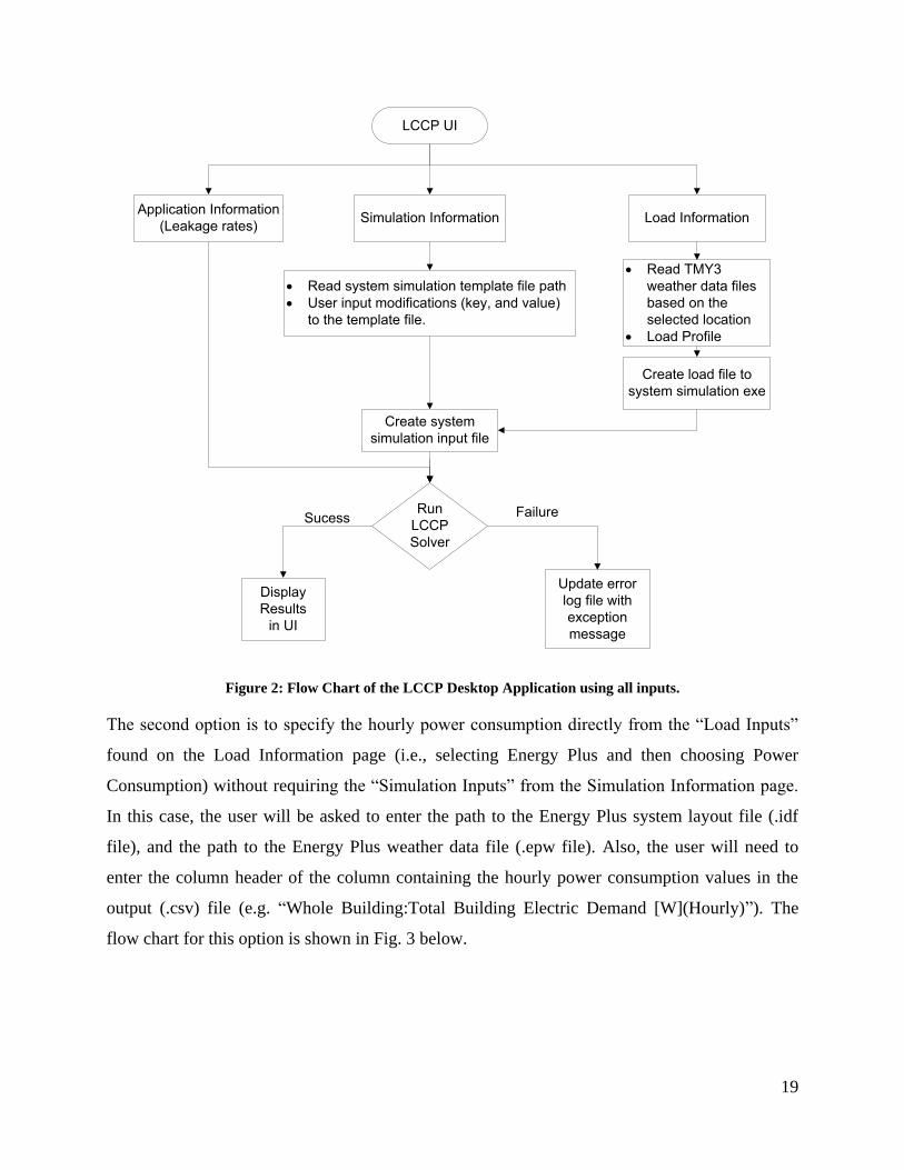
8. LCCP Tool Flow Charts

The LCCP desktop software provides three different options for specifying the system’s hourly

load or power consumption. The first option is through obtaining the hourly load using the “Load

Inputs” found on the Load Information page (i.e., built in, user input absolute load values file,

user input load percentage file, Energy Plus software for load calculation). When using this

option, the user must provide the “Simulation Inputs” (found on the Simulation Information

page) that are required to run the system simulation software (e.g. VapCyc). The flow chart for

this option is shown in Fig. 2 below.

19

RunLCCPSolver

· Read TMY3 weather data files based on the selected location

· Load Profile

Display Results

in UI

Update error log file with exception message

Sucess Failure

Create load file to system simulation exe

· Read system simulation template file path· User input modifications (key, and value)

to the template file.

Create system simulation input file

Load InformationApplication Information(Leakage rates) Simulation Information

LCCP UI

Figure 2: Flow Chart of the LCCP Desktop Application using all inputs.

The second option is to specify the hourly power consumption directly from the “Load Inputs”

found on the Load Information page (i.e., selecting Energy Plus and then choosing Power

Consumption) without requiring the “Simulation Inputs” from the Simulation Information page.

In this case, the user will be asked to enter the path to the Energy Plus system layout file (.idf

file), and the path to the Energy Plus weather data file (.epw file). Also, the user will need to

enter the column header of the column containing the hourly power consumption values in the

output (.csv) file (e.g. “Whole Building:Total Building Electric Demand [W](Hourly)”). The

flow chart for this option is shown in Fig. 3 below.

20

RunLCCPSolver

Display Results

in UI

Update error log file with exception message

Sucess Failure

EnergyPlus Load Information

Application Information(Leakage rates)

LCCP UI

Figure 3: Flow Chart of the LCCP Desktop Application using Energy Plus for power consumption

calculation.

The third option is to specify the hourly power consumption directly from the “Simulation

Information” without requiring the “Load Information”. This case is applicable to the “Display

Cases Using Secondary Refrigerants” and the “Water Chiller” systems. The flow chart for this

option is shown in Fig. 4 below.

21

RunLCCPSolver

Display Results

in UI

Update error log file with exception message

Sucess Failure

Simulation Information

Application Information(Leakage rates)

LCCP UI

Figure 4: Flow Chart of the LCCP Desktop Application with no load information required.

9. VapCyc Executable

This section covers the use of VapCyc as the system simulation software. This is just an example

to demonstrate how the system simulation software is used. Other system simulation software

can be used with LCCP tool. It is also worth mentioning that VapCyc is not part of the open

source license of the LCCP desktop tool.

The VapCyc executable requires the following three inputs: the path to the file containing the

hourly load and weather data, the path to the VapCyc input file, and the path to the output file

into which the output will be written.

Initially, the VapCyc executable reads the weather data and load data from the first input file.

Then, the weather data is placed into bins. That is, the ambient temperatures are divided into

ranges, or bins, of 10 °C and the number of hours for which the temperature falls within each bin

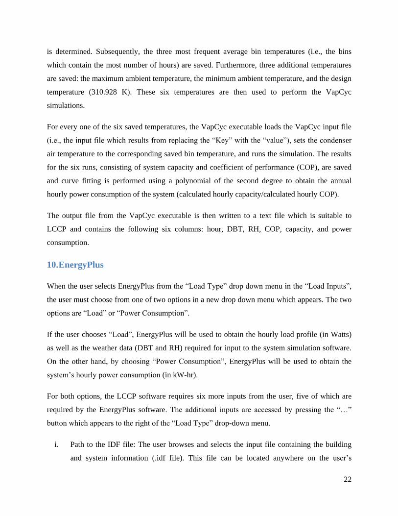
22

is determined. Subsequently, the three most frequent average bin temperatures (i.e., the bins

which contain the most number of hours) are saved. Furthermore, three additional temperatures

are saved: the maximum ambient temperature, the minimum ambient temperature, and the design

temperature (310.928 K). These six temperatures are then used to perform the VapCyc

simulations.

For every one of the six saved temperatures, the VapCyc executable loads the VapCyc input file

(i.e., the input file which results from replacing the “Key” with the “value”), sets the condenser

air temperature to the corresponding saved bin temperature, and runs the simulation. The results

for the six runs, consisting of system capacity and coefficient of performance (COP), are saved

and curve fitting is performed using a polynomial of the second degree to obtain the annual

hourly power consumption of the system (calculated hourly capacity/calculated hourly COP).

The output file from the VapCyc executable is then written to a text file which is suitable to

LCCP and contains the following six columns: hour, DBT, RH, COP, capacity, and power

consumption.

10. EnergyPlus

When the user selects EnergyPlus from the “Load Type” drop down menu in the “Load Inputs”,

the user must choose from one of two options in a new drop down menu which appears. The two

options are “Load” or “Power Consumption”.

If the user chooses “Load”, EnergyPlus will be used to obtain the hourly load profile (in Watts)

as well as the weather data (DBT and RH) required for input to the system simulation software.

On the other hand, by choosing “Power Consumption”, EnergyPlus will be used to obtain the

system’s hourly power consumption (in kW-hr).

For both options, the LCCP software requires six more inputs from the user, five of which are

required by the EnergyPlus software. The additional inputs are accessed by pressing the “…”

button which appears to the right of the “Load Type” drop-down menu.

i. Path to the IDF file: The user browses and selects the input file containing the building

and system information (.idf file). This file can be located anywhere on the user’s

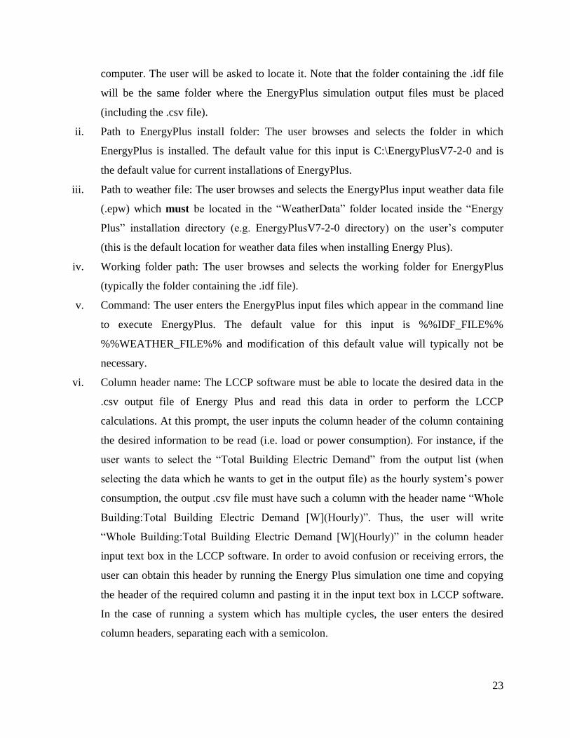
23

computer. The user will be asked to locate it. Note that the folder containing the .idf file

will be the same folder where the EnergyPlus simulation output files must be placed

(including the .csv file).

ii. Path to EnergyPlus install folder: The user browses and selects the folder in which

EnergyPlus is installed. The default value for this input is C:\EnergyPlusV7-2-0 and is

the default value for current installations of EnergyPlus.

iii. Path to weather file: The user browses and selects the EnergyPlus input weather data file

(.epw) which must be located in the “WeatherData” folder located inside the “Energy

Plus” installation directory (e.g. EnergyPlusV7-2-0 directory) on the user’s computer

(this is the default location for weather data files when installing Energy Plus).

iv. Working folder path: The user browses and selects the working folder for EnergyPlus

(typically the folder containing the .idf file).

v. Command: The user enters the EnergyPlus input files which appear in the command line

to execute EnergyPlus. The default value for this input is %%IDF_FILE%%

%%WEATHER_FILE%% and modification of this default value will typically not be

necessary.

vi. Column header name: The LCCP software must be able to locate the desired data in the

.csv output file of Energy Plus and read this data in order to perform the LCCP

calculations. At this prompt, the user inputs the column header of the column containing

the desired information to be read (i.e. load or power consumption). For instance, if the

user wants to select the “Total Building Electric Demand” from the output list (when

selecting the data which he wants to get in the output file) as the hourly system’s power

consumption, the output .csv file must have such a column with the header name “Whole

Building:Total Building Electric Demand [W](Hourly)”. Thus, the user will write

“Whole Building:Total Building Electric Demand [W](Hourly)” in the column header

input text box in the LCCP software. In order to avoid confusion or receiving errors, the

user can obtain this header by running the Energy Plus simulation one time and copying

the header of the required column and pasting it in the input text box in LCCP software.

In the case of running a system which has multiple cycles, the user enters the desired

column headers, separating each with a semicolon.

24

It is worth mentioning that since the hourly data is required, when selecting the data to be

reported in the EnergyPlus output from the IDF editor tool, the “reporting frequency” should be

set to either “Hourly” or “Time Step” with the time step being set to 1 hour. Also, if EnergyPlus

is used for load calculation rather than power consumption calculation, the DBT and the RH of

the outdoor air should be selected when the user is selecting the data to be reported in the

EnergyPlus output from the IDF editor tool.

Finally, the user should ensure that the number of cycles in the system selected in the “System

Inputs” should be equal to the number of cycles in EnergyPlus.

25

Part 3: Interfaces

11. LCCP interfaces

The LCCP code has 4 different interfaces:

1. ILCCPApplicationInfo

2. ILCCPSystem

3. ILCCPSolver

4. ILCCPResults

The “ILCCPApplicationInfo” is responsible for the “Application Information” inputs which are

explained in section 5. This interface has 1 Bolean check, and 3 main methods in it. A summary

of these methods is shown in Table 2. The Boolean check is “Initialize” which is true if

application information is initialized properly. The first method is the

“GetUnitPowerPlantEmissions” method which returns the hourly Emissions per unit Energy for

the location. The other method is the “GetLoadValues” which is responsible for returning the

hourly DBT, dew point temperature, RH, and absolute load values (in W) to the LCCP solver.

The third method is the “GetEnergyConsumption” which returns the actual hourly energy

consumption for each cycle in the system. Currently, the ILCCPApplicationInfo is implemented

in 3 different classes in the distributed version of the LCCP desktop software. The first class is

the “LCCPApplicationBase” class for built-in load type (see section 6.1.1) and file based load

type (see section 6.1.2), while the second one is the “EPApplicationInfo” for the EnergyPlus load

type (see sections 6.1.3 and 10), and the third one is the “ASHPApplicationInfo” for the AHRI

Standard load type (see section 6.1.4). Each of the first two classes initialize the LCCP

application (reads the TMY# weather file, TMY# emissions data file, and the load values .csv

file), sets the required inputs for load calculation, and outputs the weather data and load values.

In addition, this interface has 2 methods for saving and loading the application information xml

node in the lccp file.

26

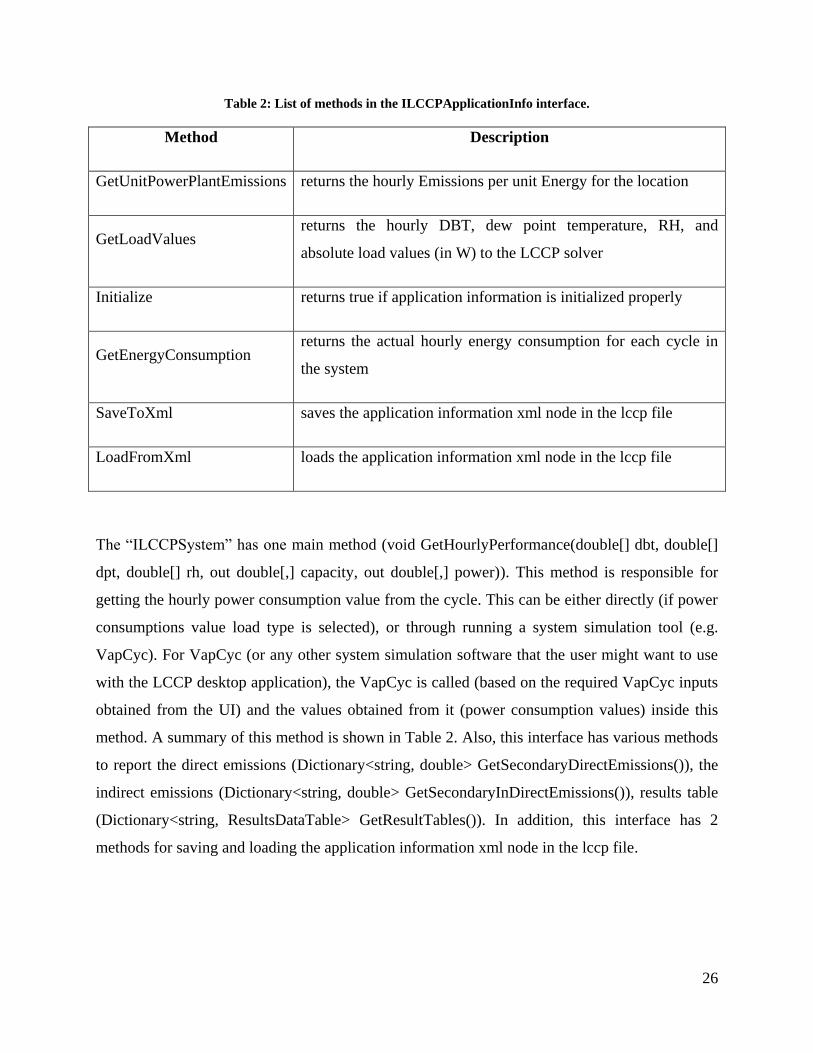
Table 2: List of methods in the ILCCPApplicationInfo interface.

Method Description

GetUnitPowerPlantEmissions returns the hourly Emissions per unit Energy for the location

GetLoadValues returns the hourly DBT, dew point temperature, RH, and

absolute load values (in W) to the LCCP solver

Initialize returns true if application information is initialized properly

GetEnergyConsumption returns the actual hourly energy consumption for each cycle in

the system

SaveToXml saves the application information xml node in the lccp file

LoadFromXml loads the application information xml node in the lccp file

The “ILCCPSystem” has one main method (void GetHourlyPerformance(double[] dbt, double[]

dpt, double[] rh, out double[,] capacity, out double[,] power)). This method is responsible for

getting the hourly power consumption value from the cycle. This can be either directly (if power

consumptions value load type is selected), or through running a system simulation tool (e.g.

VapCyc). For VapCyc (or any other system simulation software that the user might want to use

with the LCCP desktop application), the VapCyc is called (based on the required VapCyc inputs

obtained from the UI) and the values obtained from it (power consumption values) inside this

method. A summary of this method is shown in Table 2. Also, this interface has various methods

to report the direct emissions (Dictionary<string, double> GetSecondaryDirectEmissions()), the

indirect emissions (Dictionary<string, double> GetSecondaryInDirectEmissions()), results table

(Dictionary<string, ResultsDataTable> GetResultTables()). In addition, this interface has 2

methods for saving and loading the application information xml node in the lccp file.

27

Table 3: List of methods in the ILCCPSystem interface.

Method Description

GetHourlyPerformance returns the hourly power consumption value from the cycle

GetSecondaryDirectEmissions Reports the named direct emissions calculated as a part of the

system

GetSecondaryInDirectEmissions Reports the named indirect emissions calculated as a part of

the system

GetResultTables Reports the results table

SaveToXml saves the simulation information xml node in the lccp file

LoadFromXml loads the simulation information xml node in the lccp file

The “ILCCPSolver” has two methods methods. The first one has a Boolean return (bool

SetLCCPInputs(ILCCPSystem system, ILCCPApplicationInfo appInfo, BasicSystemInputs

inputs)). This method is responsible for changing the basic system inputs which are received

from the user through the UI to LCCP inputs (in the form of application and system inputs). The

basic system inputs (from the “BasicSystemInputs” class) contain the city name “City”, system

life time “LifetimeYrs”, number of cycles in the system “CycleCount”, different emission inputs

“emmInputs” (CO2 equivalent and GWP), and the different cycle inputs “inputs” (from the

“CycleInputs” class). The cycle inputs include the system type, refrigerant name, charge,

nominal load, different leakage rates, and the mass of the different materials in the system. The

main class which implements this interface is the “LCCPSolver” class. This class contains a

method “CalculateIndirectFromEnergy” which obtains the hourly performance (from the

“GetLoadValues” and the “GetHourlyPerformance” methods) and then obtains the hourly energy

consumption of the cycle (based on its refrigeration capacity and power consumption required).

The different cycle emissions (i.e. LCCP core calculation for direct and indirect emissions) are

28

performed in this class. The second method is the Run method which returns the LCCP results. A

summary of these 2 method is shown in Table 3.

Table 4: List of methods in the ILCCPSolver interface.

Method Description

SetLCCPInputs

changes the basic system inputs which are

received from the user through the UI to LCCP

inputs

Run returns the LCCP results

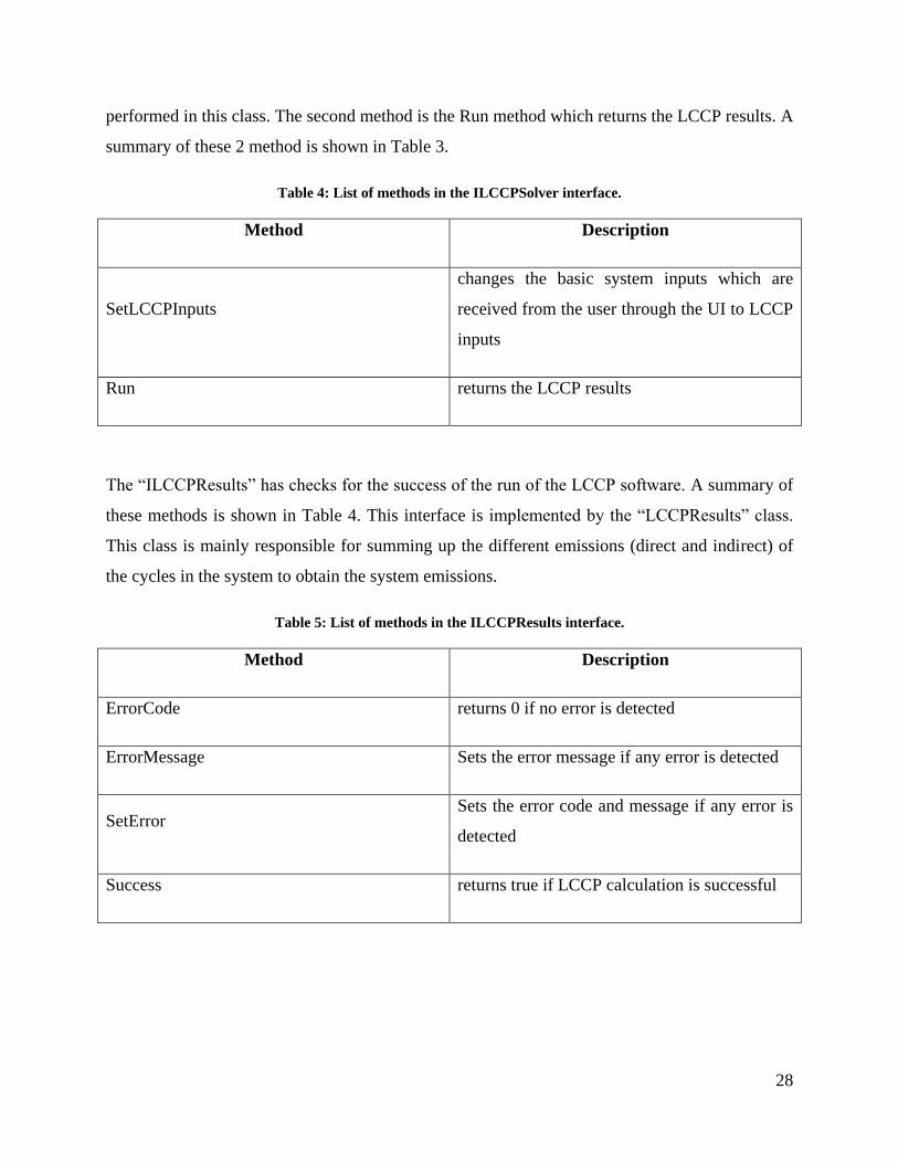
The “ILCCPResults” has checks for the success of the run of the LCCP software. A summary of

these methods is shown in Table 4. This interface is implemented by the “LCCPResults” class.

This class is mainly responsible for summing up the different emissions (direct and indirect) of

the cycles in the system to obtain the system emissions.

Table 5: List of methods in the ILCCPResults interface.

Method Description

ErrorCode returns 0 if no error is detected

ErrorMessage Sets the error message if any error is detected

SetError Sets the error code and message if any error is

detected

Success returns true if LCCP calculation is successful

29

References

ANSI/AHRI, 2011. ANSI/AHRI 1320-2011, Performance Rating of Commercial Refrigerated

Display Merchandisers and Storage Cabinets for Use With Secondary Refrigerants.

ANSI/AHRI, 2011. ANSI/AHRI 550/590-2011 with Addendum 1, Performance Rating Of

Water-Chilling and Heat Pump Water-Heating Packages Using the Vapor Compression Cycle.

ANSI/AHRI, 2008. ANSI/AHRI 210/240-2008 with Addenda 1 and 2, Performance Rating of

Unitary Air-Conditioning & Air-Source Heat Pump Equipment.

Deru, M., and Torcellini, P. 2007. Source Energy and Emission Factors for Energy Use in

Buildings. NREL Technical Report NREL/TP-550-38617. National Renewable Energy

Laboratory: Golden, CO.

Hwang, Y., Jin, D.-H., and Radermacher, R. 2007. Comparison of R-290 and two HFC blends

for walk-in refrigeration systems. International Journal of Refrigeration 30(4): 633-641.

NREL. 2012a. National Solar Radiation Data Base, 1991-2005 Update: Typical Meteorological

Year 3. Renewable Resource Data Center, National Renewable Energy Laboratory: Golden, CO.

Available at: http://rredc.nrel.gov/solar/old_data/nsrdb/19912005/tmy3/by_state_and_city.html

NREL. 2012b. U.S. Life Cycle Inventory Database. National Renewable Energy Laboratory:

Golden, CO. Available at: http://www.nrel.gov/lci/

Papasavva, S., Hill, W.R., and Andersen, S.O. 2010. GREEN-MAC-LCCP: A Tool for

Assessing the Life Cycle Climate Performance of MAC Systems. Environmental Science &

Technology 44(19): 7666-7672.

Sand, J.R., Fischer, S.K., and Baxter, V.D. 1997. Energy and Global Warming Impacts of HFC

Refrigerants and Emerging Technologies: TEWI-III. Presented at the International Conference

on Climate Change, Baltimore, MD, 12-13 June 1997.