Language-Directed Hardware Design for Network Performance ...sn624/papers/marple-sigcomm17.pdf ·...
14
Language-Directed Hardware Design for Network Performance Monitoring Srinivas Narayana 1 , Anirudh Sivaraman 1 , Vikram Nathan 1 , Prateesh Goyal 1 , Venkat Arun 2 , Mohammad Alizadeh 1 , Vimalkumar Jeyakumar 3 , Changhoon Kim 4 1 MIT CSAIL 2 IIT Guwahati 3 Cisco Tetration Analytics 4 Barefoot Networks ABSTRACT Network performance monitoring today is restricted by existing switch support for measurement, forcing operators to rely heavily on endpoints with poor visibility into the network core. Switch vendors have added progressively more monitoring features to switches, but the current trajectory of adding specific features is unsustainable given the ever-changing demands of network operators. Instead, we ask what switch hardware primitives are required to support an expressive language of network performance questions. We believe that the resulting switch hardware design could address a wide variety of current and future performance monitoring needs. We present a performance query language, Marple, modeled on fa- miliar functional constructs like map, filter, groupby, and zip. Marple is backed by a new programmable key-value store primitive on switch hardware. The key-value store performs flexible aggregations at line rate (e.g., a moving average of queueing latencies per flow), and scales to millions of keys. We present a Marple compiler that targets a P4-programmable software switch and a simulator for high- speed programmable switches. Marple can express switch queries that could previously run only on end hosts, while Marple queries only occupy a modest fraction of a switch’s hardware resources. CCS CONCEPTS • Networks → Network monitoring; Programmable networks; KEYWORDS Network measurement; network hardware; network programming ACM Reference format: Srinivas Narayana, Anirudh Sivaraman, Vikram Nathan, Prateesh Goyal, Venkat Arun, Mohammad Alizadeh, Vimalkumar Jeyakumar, and Changhoon Kim. 2017. Language-Directed Hardware Design for Network Performance Monitoring. In Proceedings of SIGCOMM ’17, Los Angeles, CA, USA, August 21–25, 2017, 14 pages. https://doi.org/10.1145/3098822.3098829 Permission to make digital or hard copies of all or part of this work for personal or classroom use is granted without fee provided that copies are not made or distributed for profit or commercial advantage and that copies bear this notice and the full citation on the first page. Copyrights for components of this work owned by others than the author(s) must be honored. Abstracting with credit is permitted. To copy otherwise, or republish, to post on servers or to redistribute to lists, requires prior specific permission and/or a fee. Request permissions from [email protected]. SIGCOMM ’17, August 21–25, 2017, Los Angeles, CA, USA © 2017 Copyright held by the owner/author(s). Publication rights licensed to Association for Computing Machinery. ACM ISBN 978-1-4503-4653-5/17/08. . . $15.00 https://doi.org/10.1145/3098822.3098829 1 INTRODUCTION Effective performance monitoring of large networks is crucial to quickly localize problems like high queueing latency [12], TCP in- cast [61], and load imbalance across network links [27]. A common approach to network monitoring is to collect information from the endpoint network stack [53, 58, 62] or to use end-to-end probes [40] to diagnose performance problems. While endpoints provide appli- cation context, they lack visibility to localize performance problems at links deep in the network. For example, it is challenging to local- ize queue buildup to a particular switch or pinpoint traffic causing the queue buildup, forcing operators to infer the network-level root causes indirectly [40]. Switch-based monitoring could allow operators to diagnose prob- lems with more direct visibility into performance statistics. How- ever, traditional switch mechanisms like sampling [7, 21], mirror- ing [8, 42, 65], and counting [34, 49] are quite restrictive. Sampling and mirroring miss events of interest as it is infeasible to collect information on all packets, while counters only track traffic volume statistics. None of these mechanisms provides relevant performance data, like queueing delays. Some upcoming technologies recognize the need for better perfor- mance monitoring using switches. In-band network telemetry [12] writes queueing delays experienced by a packet on the packet itself, allowing endpoints to localize delay spikes. The Tetration switching chip [9] provides a flow cache that measures flow-level performance metrics. These metrics are useful, but they are exposed at a fixed granularity (e.g., per 5-tuple), and the metrics themselves are fixed. For example, the list of exposed metrics includes flow-level latency and packet size variation, but not latency variation, i.e., jitter. Operator requirements are ever-changing, and redesigning hard- ware is expensive. We believe that the trajectory of adding fixed- function switch monitoring piecemeal is unsustainable. Instead, we advocate building performance monitoring primitives that can be flexibly reused for a variety of needs. Programmable switches [3, 13, 25] now support flexible parsing [39], header processing [33, 56], and scheduling [57]. Our goal is to add monitoring to this list. This paper applies language-directed hardware design to the problem of flexible performance monitoring, inspired by early efforts on designing hardware to support high-level languages [36, 50, 59]. Specifically, we design a language that can express a broad variety of performance monitoring use cases, and then design high-speed switch hardware primitives in service of this language. By designing hardware to support an expressive language, we believe the resulting hardware design can support a wide variety of current and future performance monitoring needs. Fig. 1 provides an overview of our performance monitoring sys- tem. To use the system, an operator writes a query in a domain- specific language called Marple, either to implement a long-running
Transcript of Language-Directed Hardware Design for Network Performance ...sn624/papers/marple-sigcomm17.pdf ·...
Language-Directed Hardware Design forNetwork Performance Monitoring
Srinivas Narayana1, Anirudh Sivaraman1, Vikram Nathan1, Prateesh Goyal1,Venkat Arun2, Mohammad Alizadeh1, Vimalkumar Jeyakumar3, Changhoon Kim4
1 MIT CSAIL 2 IIT Guwahati 3 Cisco Tetration Analytics 4 Barefoot Networks
ABSTRACTNetwork performance monitoring today is restricted by existingswitch support for measurement, forcing operators to rely heavily onendpoints with poor visibility into the network core. Switch vendorshave added progressively more monitoring features to switches, butthe current trajectory of adding specific features is unsustainablegiven the ever-changing demands of network operators. Instead,we ask what switch hardware primitives are required to support anexpressive language of network performance questions. We believethat the resulting switch hardware design could address a widevariety of current and future performance monitoring needs.
We present a performance query language, Marple, modeled on fa-miliar functional constructs like map, filter, groupby, and zip. Marpleis backed by a new programmable key-value store primitive onswitch hardware. The key-value store performs flexible aggregationsat line rate (e.g., a moving average of queueing latencies per flow),and scales to millions of keys. We present a Marple compiler thattargets a P4-programmable software switch and a simulator for high-speed programmable switches. Marple can express switch queriesthat could previously run only on end hosts, while Marple queriesonly occupy a modest fraction of a switch’s hardware resources.
CCS CONCEPTS• Networks→ Network monitoring; Programmable networks;
KEYWORDSNetwork measurement; network hardware; network programming
ACM Reference format:Srinivas Narayana, Anirudh Sivaraman, Vikram Nathan, Prateesh Goyal,Venkat Arun, Mohammad Alizadeh, Vimalkumar Jeyakumar, and ChanghoonKim. 2017. Language-Directed Hardware Design for Network PerformanceMonitoring. In Proceedings of SIGCOMM ’17, Los Angeles, CA, USA, August21–25, 2017, 14 pages.https://doi.org/10.1145/3098822.3098829
Permission to make digital or hard copies of all or part of this work for personal orclassroom use is granted without fee provided that copies are not made or distributedfor profit or commercial advantage and that copies bear this notice and the full citationon the first page. Copyrights for components of this work owned by others than theauthor(s) must be honored. Abstracting with credit is permitted. To copy otherwise, orrepublish, to post on servers or to redistribute to lists, requires prior specific permissionand/or a fee. Request permissions from [email protected] ’17, August 21–25, 2017, Los Angeles, CA, USA© 2017 Copyright held by the owner/author(s). Publication rights licensed to Associationfor Computing Machinery.ACM ISBN 978-1-4503-4653-5/17/08. . . $15.00https://doi.org/10.1145/3098822.3098829
1 INTRODUCTIONEffective performance monitoring of large networks is crucial toquickly localize problems like high queueing latency [12], TCP in-cast [61], and load imbalance across network links [27]. A commonapproach to network monitoring is to collect information from theendpoint network stack [53, 58, 62] or to use end-to-end probes [40]to diagnose performance problems. While endpoints provide appli-cation context, they lack visibility to localize performance problemsat links deep in the network. For example, it is challenging to local-ize queue buildup to a particular switch or pinpoint traffic causingthe queue buildup, forcing operators to infer the network-level rootcauses indirectly [40].
Switch-based monitoring could allow operators to diagnose prob-lems with more direct visibility into performance statistics. How-ever, traditional switch mechanisms like sampling [7, 21], mirror-ing [8, 42, 65], and counting [34, 49] are quite restrictive. Samplingand mirroring miss events of interest as it is infeasible to collectinformation on all packets, while counters only track traffic volumestatistics. None of these mechanisms provides relevant performancedata, like queueing delays.
Some upcoming technologies recognize the need for better perfor-mance monitoring using switches. In-band network telemetry [12]writes queueing delays experienced by a packet on the packet itself,allowing endpoints to localize delay spikes. The Tetration switchingchip [9] provides a flow cache that measures flow-level performancemetrics. These metrics are useful, but they are exposed at a fixedgranularity (e.g., per 5-tuple), and the metrics themselves are fixed.For example, the list of exposed metrics includes flow-level latencyand packet size variation, but not latency variation, i.e., jitter.
Operator requirements are ever-changing, and redesigning hard-ware is expensive. We believe that the trajectory of adding fixed-function switch monitoring piecemeal is unsustainable. Instead, weadvocate building performance monitoring primitives that can beflexibly reused for a variety of needs. Programmable switches [3, 13,25] now support flexible parsing [39], header processing [33, 56],and scheduling [57]. Our goal is to add monitoring to this list.
This paper applies language-directed hardware design to theproblem of flexible performance monitoring, inspired by early effortson designing hardware to support high-level languages [36, 50, 59].Specifically, we design a language that can express a broad varietyof performance monitoring use cases, and then design high-speedswitch hardware primitives in service of this language. By designinghardware to support an expressive language, we believe the resultinghardware design can support a wide variety of current and futureperformance monitoring needs.
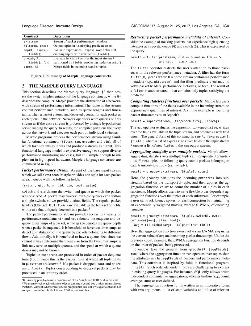
Fig. 1 provides an overview of our performance monitoring sys-tem. To use the system, an operator writes a query in a domain-specific language called Marple, either to implement a long-running

SIGCOMM ’17, August 21–25, 2017, Los Angeles, CA, USA S. Narayana et al.
Collectionserverstohandle(1)Marple queryresults(2)Evictionstobackingstore
MarpleQueries
MarpleCompiler
SwitchPrograms
Programmableswitcheswithprogrammablekey-valuestore EndhostsEndhosts
Networkoperator
Figure 1: Operators issue Marple queries, which are com-piled into switch programs for programmable switches aug-mented with our new programmable key-value store primitive.Switches stream results from this query to collection serversthat also house the backing store for the key-value store.
monitor for a statistic (e.g., detecting TCP timeouts), or to trou-bleshoot a specific problem (e.g., incast [61]) at hand. The queryis compiled into a switch program that runs on the network’s pro-grammable switches, augmented with new switch hardware primi-tives that we design in service of Marple. The switches stream resultsout to collection servers, where the operator can retrieve query re-sults. We now briefly describe the three components of our system:the query language, the switch hardware, and the query compiler.
Performance query language. Marple uses familiar functionalconstructs like map, filter, groupby and zip for performance mon-itoring. Marple provides the abstraction of a stream that containsperformance information for every packet at every queue in thenetwork (§2). Programmers can focus their attention on traffic ex-periencing interesting performance using filter (e.g., packets withhigh queueing latencies), aggregate information across packets inflexible ways using groupby (e.g., compute a moving average overqueueing latency per flow), compute new stateless quantities usingmap (e.g., binning a packet’s timestamp into an epoch), and detect si-multaneous performance conditions using zip (e.g., when the queuedepth is large and the number of connections in the queue is high).
Hardware design for performance queries. A naïve implemen-tation of Marple might stream every packet’s metadata from thenetwork to a central location and run streaming queries against it.Modern scale-out data-processing systems support 100K–1M oper-ations per second per core [2, 4, 11, 43, 64], but processing everysingle packet (assuming a relatively large packet size of 1 KB) froma single 1 Tbit/s switch would need 100M operations per second —2–3 orders of magnitude more than what existing systems support.
Instead, we leverage high-speed programmable switches [3, 13,25, 33] as first-class citizens in network monitoring, because theycan programmatically manipulate multi-Tbit/s packet streams. Earlyfiltering and flexible aggregation on switches drastically reduce
the number of records per second streamed out to a standard data-processing system running on the collection server.
While programmable switches support many of Marple’s statelesslanguage constructs that modify packet fields alone (e.g., map andfilter), they do not support aggregation of state across packets fora large number of flows (i.e., groupby). To support flexible aggre-gations over packets, we design a programmable key-value storein hardware (§3), where the keys represent flow identifiers and thevalues represent the state computed by the aggregation function.This key-value store must update values at the line rate of 1 packetper clock cycle (at 1 GHz [6, 33]) and support millions of keys (i.e.,flows). Unfortunately, neither SRAM nor DRAM is simultaneouslyfast and dense enough to meet both requirements.
We split the key-value store into a small but fast on-chip cachein SRAM and a larger but slower off-chip backing store in DRAM.Traditional caches incur variable write latencies due to cache misses;however, line-rate packet forwarding requires deterministic latencyguarantees. Our design accomplishes this by never reading back avalue into the cache if it has already been evicted to the backingstore. Instead, it treats a cache miss as the arrival of a packet from anew flow. When a flow is evicted, we merge the evicted flow’s valuein the cache with the flow’s old value in the backing store. Becausemerges occur off the critical packet processing path, the backingstore can be implemented in software on a separate collection server.
While it is not always possible to merge an aggregation functionwithout losing accuracy, we characterize a class of affine aggregationfunctions, which we call linear-in-state, for which accurate mergingis possible. Many useful aggregation functions are linear-in-state,e.g., counters, predicated counters (e.g., count only TCP packetsthat saw timeouts), exponentially weighted moving averages, andfunctions computed over a finite window of packets. We design aswitch instruction to support linear-in-state functions, finding that iteasily meets timing at 1 GHz, while occupying modest silicon area.
Query compiler. We implement a compiler that takes Marplequeries and compiles them into switch configurations for two tar-gets (§4): (1) the P4 behavioral model [19], an open source pro-grammable software switch that can be used for end-to-end evalu-ations of Marple on Mininet [47], and (2) Banzai [56], a simulatorfor high-speed programmable switch hardware that can be used toexperiment with different instruction sets. The Marple compiler de-tects linear-in-state aggregations in input queries and successfullytargets the linear-in-state switch instruction that we add to Banzai.
Evaluation. We show that Marple can express a variety of use-ful performance monitoring examples, like detecting and localiz-ing TCP incast and measuring the prevalence of out-of-order TCPpackets. Marple queries require between 4 and 11 pipeline stages,which is modest for a 32-stage switch pipeline [33]. We evalu-ate our key-value store’s performance using trace-driven simula-tions. For a 64 Mbit on-chip cache, which occupies about 10% ofthe area of a 64×10-Gbit/s switching chip, we estimate that thecache eviction rate from a single top-of-rack switch can be han-dled by a single 8-core server running Redis [20]. We evaluateMarple’s usability through two Mininet case studies that use Marpleto troubleshoot high tail latencies [26] and measure the distribu-tion of flowlet sizes [27]. Marple is open source and available athttp://web.mit.edu/marple.
Language-Directed Hardware Design SIGCOMM ’17, August 21–25, 2017, Los Angeles, CA, USA
Construct Descriptionpktstream Stream of packet performance metadata.filter(R, pred) Output tuples in R satisfying predicate pred.map(R, [exprs], Evaluate expressions, [exprs], over fields of R,[fields]) emitting tuples with new fields, [fields].
groupby(R, Evaluate function fun over the input stream R
[fields], fun) partitioned by fields, producing tuples on emit().
zip(R, S) Merge fields in incoming R and S tuples.
Figure 2: Summary of Marple language constructs.
2 THE MARPLE QUERY LANGUAGEThis section describes the Marple query language. §3 then cov-ers the switch implementation of the language constructs, while §4describes the compiler. Marple provides the abstraction of a network-wide stream of performance information. The tuples in the streamcontain performance metadata, such as queue lengths and times-tamps when a packet entered and departed queues, for each packet ateach queue in the network. Network operators write queries on thisstream as if the entire stream is processed by a single hypotheticalserver running the query. In reality, the compiler partitions the queryacross the network and executes each part on individual switches.
Marple programs process the performance stream using famil-iar functional constructs (filter, map, groupby, and zip), all ofwhich take streams as inputs and produce a stream as output. Thisfunctional language model is expressive enough to support diverseperformance monitoring use cases, but still simple enough to im-plement in high-speed hardware. Marple’s language constructs aresummarized in Fig. 2.
Packet performance stream. As part of the base input stream,which we call pktstream, Marple provides one tuple for each packetat each queue with the following fields.
(switch, qid, hdrs, uid, tin, tout, qsize)
switch and qid denote the switch and queue at which the packetwas observed. A packet may traverse multiple queues even withina single switch, so we provide distinct fields. The regular packetheaders (Ethernet, IP, TCP, etc.) are available in the hdrs set of fields,with a uid that uniquely determines a packet.1
The packet performance stream provides access to a variety ofperformance metadata: tin and tout denote the enqueue and de-queue timestamps of a packet, while qsize denotes the queue depthwhen a packet is enqueued. It is beneficial to have two timestamps todetect co-habitation of the queue by packets belonging to differentflows. Additionally, it is beneficial to have a queue size, since wecannot always determine the queue size from the two timestamps: alink may service multiple queues, and the speed at which a queuedrains may not be known.
Tuples in pktstream are processed in order of packet dequeuetime (tout), since this is the earliest time at which all tuple fieldsin pktstream are known.2 If a packet is dropped, tout and qsize
are infinity. Tuples corresponding to dropped packets may beprocessed in an arbitrary order.
1It is usually possible to use a combination of the 5-tuple and IP ID field as the uid.2We assume clock synchronization to let us compare tin and tout values from differentswitches. Without synchronization, the programmer can still write queries that do notcompare time-valued fields tin and tout across switches.
Restricting packet performance metadata of interest. Con-sider the example of tracking packets that experience high queueinglatencies at a specific queue (Q) and switch (S). This is expressed bythe query:
result = filter(pktstream, qid == Q and switch == S
and tout - tin > 1ms)
The filter operator restricts the user’s attention to those pack-ets with the relevant performance metadata. A filter has the formfilter(R, pred) where R is some stream containing performancemetadata (e.g., pktstream), and the filter predicate pred may in-volve packet headers, performance metadata, or both. The result ofa filter is another stream that contains only tuples satisfying thepredicate.
Computing stateless functions over packets. Marple lets userscompute functions of the fields available in the incoming stream, toexpress new quantities of interest. A simple example is roundingpacket timestamps to an ‘epoch’:
result = map(pktstream, [tin/epoch_size], [epoch]);
The map operator evaluates the expression tin/epoch_size, writtenover the fields available in the tuple stream, and produces a new fieldepoch. The general form of this construct is map(R, [expression],
[field]) where a list of expressions over fields in the input streamR creates a list of new fields in the map output stream.
Aggregating statefully over multiple packets. Marple allowsaggregating statistics over multiple tuples at user-specified granular-ities. For example, the following query counts packets belonging toeach transport-level flow (i.e., 5-tuple):
result = groupby(pktstream, [5tuple], count)
Here, the groupby partitions the incoming pktstream into sub-streams based on the transport 5-tuple, and then applies the ag-gregation function count to count the number of tuples in eachsubstream. Marple allows users to write flexible order-dependent ag-gregation functions over the tuples of each substream. For example,a user can track latency spikes for each connection by maintainingan exponentially weighted moving average (EWMA) of queueinglatencies:
result = groupby(pktstream, [5tuple, switch], ewma);
def ewma([avg], [tin, tout]):
avg = ((1-alpha)*avg) + (alpha*(tout-tin));
Here the aggregation function ewma evolves an EWMA avg usingthe current value of avg and incoming packet timestamps. Unlike theprevious count example, the EWMA aggregation function dependson the order of packets being processed.
groupbys take the general form groupby(R, [aggFields],
fun), where the aggregation function fun operates over tuples shar-ing attributes in a list aggFields of headers and performance meta-data. This construct is inspired by folds in functional program-ming [45]. Such order-dependent folds are challenging to expressin existing query languages. For instance, SQL only allows order-independent commutative aggregations, whether built-in (e.g., count,average, sum) or user-defined.
The aggregation function fun is written in an imperative form,with two arguments: a list of state variables and a list of relevant
SIGCOMM ’17, August 21–25, 2017, Los Angeles, CA, USA S. Narayana et al.
incoming tuple fields. Each statement in fun can be an assignmentto an expression (x = ...), a branching statement (if pred {...}
else {...}), or a special emit() statement that controls the outputstream of the groupby. Below, we show an example of an aggrega-tion that detects a new connection:
result = groupby(pktstream, [5tuple], new_flow);
def new_flow([fcount], []):
if fcount == 0:
fcount = 1
emit()
The output of a groupby is a stream containing the aggregation fields(e.g., 5-tuple) and the aggregated values (e.g., fcount). The outputstream contains only tuples for which the emit() statement is en-countered during execution of the aggregation function. For example,the output stream of new_flow consists of the first packet of everynew transport-level connection. If the function has no emit()s, theuser can still read the aggregated fields and their current aggregatedstate values as a table.
Chaining together multiple queries. Because all Marple con-structs produce and consume streams, Marple allows users to writequeries that take in the results of previous queries as inputs. A streamof tuples flows from one query to the next, and each query may addor filter out information from the incoming tuple, or even drop thetuple entirely. For example, the program below tracks the size dis-tribution of flowlets, i.e., bursts of packets from the same 5-tupleseparated by more than a fixed time amount delta.
fl_track = groupby(pktstream, [5tuple], fl_detect);
def fl_detect([last_time, size], [tin]):
if (tin - last_time > delta):
emit()
size = 1
else:
size = size + 1
last_time = tin
The function fl_detect detects new flowlets using the last time apacket from the same flow was seen. Because of the emit() state-ment’s location, the flowlet size from fl_track is only streamed outto other operators upon seeing the first packet of a new flowlet.
fl_bkts = map(fl_track, [size/16], [bucket]);
fl_hist = groupby(fl_bkts, [bucket], count);
The map fl_bkts bins the flowlet size emitted by fl_track into abucket index, which is used to count the number of flowlets in thecorresponding bucket in fl_hist.
Joining results across queries. Marple provides a zip operatorthat “joins” the results of two queries to check whether two condi-tions hold simultaneously. Consider the example of detecting thefan-in of packets from many connections into a single queue, charac-teristic of TCP incast [61]. This can be checked by combining twodistinct conditions: (1) the number of active flows in a queue over ashort interval of time is high, and (2) the queue occupancy is large.
A user can first compute the number of active flows over thecurrent epoch using two aggregations:
R1 = map(pktstream, [tin/epoch_size], [epoch]);
R2 = groupby(R1, [5tuple, epoch], new_flow);
R3 = groupby(R2, [epoch], count);
The number of active flows in this epoch can be combined with thequeue occupancy information in the original packet stream throughthe zip operator:
R4 = zip(R3, pktstream);
result = filter(R4, qsize > 100 and count > 25);
The result of a zip operation over two input streams is a singlestream containing tuples that are a concatenation of all the fields inthe two streams, whenever both input streams contain valid tuplesprocessed from the same original packet tuple. A zip is a specialkind of stream join where the result can be computed without havingto synchronize the two streams, because tuples of both streamsoriginate from pktstream. The result of the zip can be processedlike any other stream: the filter in the result query checks thetwo incast conditions above.
We did not find a need for more general joins akin to joins instreaming query languages like CQL [30]. Streaming joins havesemantics that can be quite complex and may produce large results,i.e., O(#pkts2). Hence, Marple restricts users to simple zip joins.
We show several examples of Marple queries in Fig. 7. For in-stance, Marple can express measurements of simple counters, TCPreordering of various forms, high-loss connections, flows with highend-to-end network latencies, and TCP fan-in.
Restrictions on Marple queries. Some aggregations are chal-lenging to implement over a network-wide stream. For example,consider an EWMA over some packet field across all packets seenanywhere in the entire network, while processing packets in the orderof their tout values. Even with clock synchronization, this aggrega-tion is hard to implement because it requires us to either coordinatebetween switches or stream all packets to a central location.
Marple’s compiler rejects queries with aggregations that need toprocess multiple packets at multiple switches in order of their toutvalues. Concretely, we only allow aggregations that relax one ofthese three conditions, and thus either
(1) operate independently on each switch, in which case we natu-rally partition queries by switch (e.g., a per-flow EWMA ofqueueing latencies on a particular switch), or
(2) operate independently on each packet, in which case we havethe packet perform the coordination by carrying the aggre-gated state to the next switch on its path (e.g., a rolling averagelink utilization seen by the packet along its path), or
(3) are associative and commutative, in which case independentswitch-local results can be combined in any order to producea correct overall result for the network [15], e.g., a count ofhow many times packets from a flow appeared throughout thenetwork. In this case, we rely on the programmer to annotatethe aggregation function with the assoc and comm keywords.
3 SCALABLE AGGREGATION AT LINE RATEHow should switches implement Marple’s language constructs? Werequire instructions on switches that can aggregate packets intoper-flow state (groupby), transform packet fields (map), stream onlypackets matching a predicate (filter), or merge packets that satisfytwo previous queries (zip).
Language-Directed Hardware Design SIGCOMM ’17, August 21–25, 2017, Los Angeles, CA, USA
Key Value
Key Valuekey Mergeevicted
key
Key Value
Key Value
Backing store (DRAM)
Writeevictedkey
Cache (SRAM)
Cache (SRAM)
Backing store (DRAM)
Hit
Miss
Update
Initialize
key
Hit
Miss
Update
Initialize/Update
Read
Traditional cache
Marple’s design
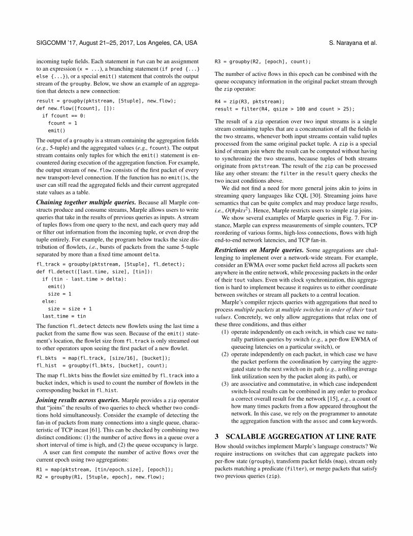
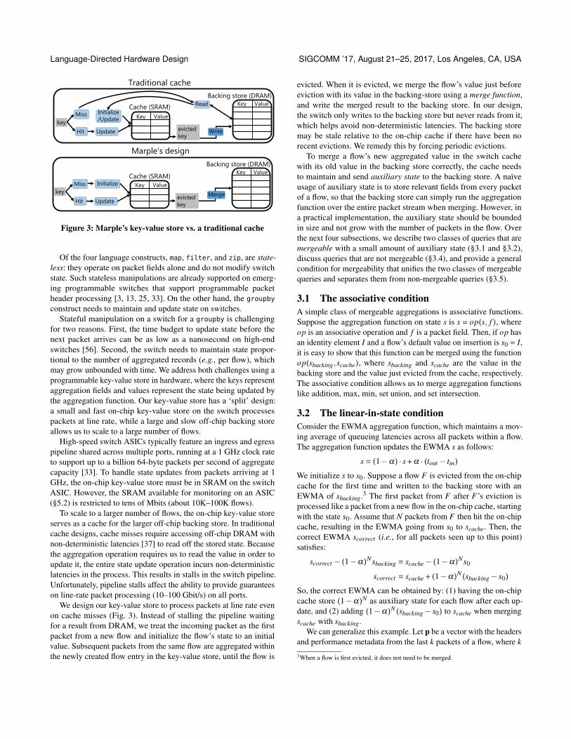
Figure 3: Marple’s key-value store vs. a traditional cache
Of the four language constructs, map, filter, and zip, are state-less: they operate on packet fields alone and do not modify switchstate. Such stateless manipulations are already supported on emerg-ing programmable switches that support programmable packetheader processing [3, 13, 25, 33]. On the other hand, the groupby
construct needs to maintain and update state on switches.Stateful manipulation on a switch for a groupby is challenging
for two reasons. First, the time budget to update state before thenext packet arrives can be as low as a nanosecond on high-endswitches [56]. Second, the switch needs to maintain state propor-tional to the number of aggregated records (e.g., per flow), whichmay grow unbounded with time. We address both challenges using aprogrammable key-value store in hardware, where the keys representaggregation fields and values represent the state being updated bythe aggregation function. Our key-value store has a ‘split’ design:a small and fast on-chip key-value store on the switch processespackets at line rate, while a large and slow off-chip backing storeallows us to scale to a large number of flows.
High-speed switch ASICs typically feature an ingress and egresspipeline shared across multiple ports, running at a 1 GHz clock rateto support up to a billion 64-byte packets per second of aggregatecapacity [33]. To handle state updates from packets arriving at 1GHz, the on-chip key-value store must be in SRAM on the switchASIC. However, the SRAM available for monitoring on an ASIC(§5.2) is restricted to tens of Mbits (about 10K–100K flows).
To scale to a larger number of flows, the on-chip key-value storeserves as a cache for the larger off-chip backing store. In traditionalcache designs, cache misses require accessing off-chip DRAM withnon-deterministic latencies [37] to read off the stored state. Becausethe aggregation operation requires us to read the value in order toupdate it, the entire state update operation incurs non-deterministiclatencies in the process. This results in stalls in the switch pipeline.Unfortunately, pipeline stalls affect the ability to provide guaranteeson line-rate packet processing (10–100 Gbit/s) on all ports.
We design our key-value store to process packets at line rate evenon cache misses (Fig. 3). Instead of stalling the pipeline waitingfor a result from DRAM, we treat the incoming packet as the firstpacket from a new flow and initialize the flow’s state to an initialvalue. Subsequent packets from the same flow are aggregated withinthe newly created flow entry in the key-value store, until the flow is
evicted. When it is evicted, we merge the flow’s value just beforeeviction with its value in the backing-store using a merge function,and write the merged result to the backing store. In our design,the switch only writes to the backing store but never reads from it,which helps avoid non-deterministic latencies. The backing storemay be stale relative to the on-chip cache if there have been norecent evictions. We remedy this by forcing periodic evictions.
To merge a flow’s new aggregated value in the switch cachewith its old value in the backing store correctly, the cache needsto maintain and send auxiliary state to the backing store. A naïveusage of auxiliary state is to store relevant fields from every packetof a flow, so that the backing store can simply run the aggregationfunction over the entire packet stream when merging. However, ina practical implementation, the auxiliary state should be boundedin size and not grow with the number of packets in the flow. Overthe next four subsections, we describe two classes of queries that aremergeable with a small amount of auxiliary state (§3.1 and §3.2),discuss queries that are not mergeable (§3.4), and provide a generalcondition for mergeability that unifies the two classes of mergeablequeries and separates them from non-mergeable queries (§3.5).
3.1 The associative conditionA simple class of mergeable aggregations is associative functions.Suppose the aggregation function on state s is s = op(s, f ), whereop is an associative operation and f is a packet field. Then, if op hasan identity element I and a flow’s default value on insertion is s0 = I,it is easy to show that this function can be merged using the functionop(sbacking,scache), where sbacking and scache are the value in thebacking store and the value just evicted from the cache, respectively.The associative condition allows us to merge aggregation functionslike addition, max, min, set union, and set intersection.
3.2 The linear-in-state conditionConsider the EWMA aggregation function, which maintains a mov-ing average of queueing latencies across all packets within a flow.The aggregation function updates the EWMA s as follows:
s = (1−α ) · s+α · (tout − tin)
We initialize s to s0. Suppose a flow F is evicted from the on-chipcache for the first time and written to the backing store with anEWMA of sbacking.3 The first packet from F after F’s eviction isprocessed like a packet from a new flow in the on-chip cache, startingwith the state s0. Assume that N packets from F then hit the on-chipcache, resulting in the EWMA going from s0 to scache. Then, thecorrect EWMA scorrect (i.e., for all packets seen up to this point)satisfies:
scorrect − (1−α )Nsbacking = scache− (1−α )Ns0
scorrect = scache + (1−α )N (sbacking− s0)
So, the correct EWMA can be obtained by: (1) having the on-chipcache store (1−α )N as auxiliary state for each flow after each up-date, and (2) adding (1−α )N (sbacking− s0) to scache when mergingscache with sbacking.
We can generalize this example. Let p be a vector with the headersand performance metadata from the last k packets of a flow, where k
3When a flow is first evicted, it does not need to be merged.
SIGCOMM ’17, August 21–25, 2017, Los Angeles, CA, USA S. Narayana et al.
is an integer determined at query compile time (§4.3). We can mergeany aggregation function with state updates of the form S = A(p) ·S+B(p), where S is the state, and A(p) and B(p) are functions ofthe last k packets. We call this condition the linear-in-state conditionand say that A(p) and B(p) are functions of bounded packet history.
The requirement of bounded packet history is important. Considerthe TCP non-monotonic query from Fig. 7, which counts the num-ber of packets with sequence numbers smaller than the maximumsequence number seen so far. The aggregation can be expressed as
count = count + (maxseq > tcpseq) ? 1 : 0
While the update superficially resembles A(p) ·S+B(p), the coeffi-cient B(p) is a function of maxseq, the maximum sequence numberso far, which could be arbitrarily far back in the stream. Intuitively,since B(p) is not a function of bounded packet history, the auxiliarystate required to merge count is large. §3.5 formalizes this intuition.
In contrast, the slightly modified TCP out-of-sequence query fromFig. 7 is linear-in-state because it can be written as
count = count + (lastseq > tcpseq) ? 1 : 0
where lastseq, the previous packet’s sequence number, dependsonly on the last 2 packets: the current and the previous packet. Here,A(p) and B(p) are functions of bounded packet history, with k = 2.
Merging queries that are linear-in-state requires the switch to storethe first k and most recent k packets for the key since it (re)appearedin the key-value store; details are available in the accompanying techreport [15]. An aggregation function is linear-in-state if, for everyvariable in the function, the state update satisfies the linear-in-statecondition. A query is linear-in-state if all its aggregation functionsare linear-in-state.
3.3 Scalable aggregation functionsA groupby with no emit() and a linear-in-state (or associative)aggregation function can be implemented scalably without losing ac-curacy. Examples of such aggregations (from Fig. 7) include trackingsuccessive packets within a TCP connection that are out-of-sequenceand counting the number of TCP timeouts per connection.
If a groupby uses an emit() to pass tuples to another query, itcannot be implemented scalably even if its aggregation function islinear-in-state or associative. An emit() outputs the current state ofthe aggregation function, which assumes the current state is alwaysavailable in the switch’s on-chip cache. This is only possible if flowsare never evicted, effectively shrinking the key-value store to itson-chip cache alone.
3.4 Handling non-scalable aggregationsWhile the linear-in-state and associative conditions capture severalaggregation functions and enable a scalable implementation, thereare two practical classes of queries that we cannot scale: (1) querieswith aggregation functions that are neither associative nor linear-in-state and (2) queries where the groupby has an emit() statement.
An example of the first class is the TCP non-monotonic querydiscussed earlier. An example of the second class is the flowlet sizehistogram query from Fig. 7, where the first groupby emits flowletsizes, which are grouped into buckets by the second groupby.
There are workarounds for non-scalable queries. One is to rewritequeries to remove emit()s. For instance, we can rewrite the loss
rate query (Fig. 7) to independently record the per-flow counts fordropped packets and total number of packets in separate key-valuestores, and have an operator consult both key-value stores everytime they need the loss rate. Each key-value store can be scaled, butthe implementation comes at a transient loss of accuracy relativeto precisely tracking the loss rate after every packet using a zip.
Second, an operator may be content with flow values that are accuratefor each time period between two evictions, but not across evictions(Fig. 10b). Third, an operator may want to run a query to collect datauntil the on-chip cache fills up and then stop data collection. Finally,if the number of keys is small enough to fit in the cache (e.g., if thekey is an application type), the system can provide accurate resultswithout evicting any keys.
3.5 A unified condition for mergeabilityWe present a general condition that separates mergeable functionsfrom non-mergeable ones. Informally, mergeable aggregation func-tions are those that maintain auxiliary state linear in the size of thefunction’s state itself. This characterization also has the benefit ofunifying the associative and linear-in-state conditions. We now for-malize our results in the form of several theorems without proofs;an accompanying technical report [15] contains the proofs.
Let n denote the size of state (in bits) tracked in a Marple query: itmust be bounded and should not increase with the number of packets.When merging state scache in the on-chip cache with state sbackingin the backing store, the switch may maintain and send auxiliarystate aux for the backing store to perform the merge correctly. In theEWMA example, the value (1−α )N is auxiliary state. Then, a mergefunction m for an aggregation function f is a function satisfying:
m(scache,aux,sbacking) = f (s0,{p1, . . . , pN})
for any N and sequence of packets p1, . . . , pN . The application of fto a list is shorthand for folding f over each packet in order.
First, we show that every aggregation function has a merge func-tion, provided it is allowed to use a large amount of auxiliary data.
THEOREM 3.1. Every aggregation function has a correspondingmerge function that uses O(n2n) auxiliary bits.
Unfortunately, memory is limited and Marple should not use muchmore state than indicated by the user’s aggregation function. We sayan aggregation function is mergeable if the auxiliary state has sizeO(n) for any sequence of packets. This characterization is consistentwith what we have described so far: the linear-in-state and associativeconditions are indeed mergeable by this definition, while queriesthat we cannot merge (e.g., TCP non-monotonic in Fig. 7) violate it.
THEOREM 3.2. If an aggregation function is either linear-in-state or associative, it has a merge function that uses O(n) bits ofauxiliary state.
THEOREM 3.3. The TCP non-monotonic query from Fig. 7 re-quires Θ(n2n) auxiliary bits in the worst case.
This raises the question: can we determine whether an aggregationfunction is mergeable with O(n) auxiliary bits? We provide an al-gorithm (described in the tech report) that computes the minimumauxiliary state size needed to merge a given aggregation function.Our current algorithm uses brute force and is doubly exponential in n.
Language-Directed Hardware Design SIGCOMM ’17, August 21–25, 2017, Los Angeles, CA, USA
However, a polynomial time algorithm is unlikely. We demonstratea hardness result by considering a decision version of a simplerversion of this problem where the merge function m is given asinput: given an aggregation function f and merge function m, doesm successfully merge f for all possible packet inputs?
THEOREM 3.4. Determining whether a merge function success-fully merges an aggregation function is co-NP-hard.
The practical implication of this result is that there is unlikely to bea general and efficient procedure to check if an arbitrary aggregationfunction can be merged using a small amount of auxiliary state.Thus, identifying specific classes of functions (e.g., linear-in-stateand associative) and checking if an aggregation function belongs tothese classes is the best we can hope to do.
3.6 Hardware feasibilityWe optimize our stateful hardware design for linear-in-state queriesand break it down into five components. Each component is well-known; our main contribution is putting them together to implementstateful queries. We now discuss each component in detail.
The on-chip cache is a hash table where each row in the hashtable stores keys and values for a certain number of flows. If a packetfrom a new flow hashes into a row that is full, the least recently usedflow within that row is evicted. Each row has 8 flows and each flowstores both its key and value.4 Our choice of 8 flows is based on8-way L1 caches, which are very common in processors [14]. Thiscache eviction policy is close to an ideal but impractical policy thatevicts the least recently used (LRU) flow across the whole table (§5).
Within a switch pipeline stage, the on-chip cache has a logicalinterface similar to an on-chip hash table used for counters: eachpacket matches entries in the table using a key extracted from thepacket header, and the corresponding action (i.e., increment) is exe-cuted by the switch. An on-chip hash table may be used as a pathto incrementally deploying a switch cache for specific aggregations(e.g., increments), on the way to supporting more general actionsand cache eviction logic in the future.
The off-chip backing store is a scale-out key-value store suchas Redis [20] running on dedicated collection servers within thenetwork. As §5 shows, the number of measurement servers requiredto support typical eviction rates from the switch’s on-chip cache issmall, even for a 64×100-Gbit/s switch.
Maintaining packet history. Before a packet reaches thepipeline stage with the on-chip cache, we use the preceding stagesto precompute A(p) and B(p) (the functions of bounded packet his-tory) in the state-update operation S = A(p) ·S+B(p). Our currentdesign only handles the case where S, A(p), and B(p) are scalars.Say A(p) and B(p) depend on packet fields from the last k packets.Then, these preceding pipeline stages act like a shift register andstore fields from the last k packets. Each stage contains a read/writeregister, which is read by a packet arriving at that stage, carried bythe packet as a header, and written into the next stage’s register. Oncevalues from the last k packets have been read into packet fields, A(p)and B(p) can be computed with stateless instructions provided byprogrammable switch architectures [33, 56].4The LRU policy is actually implemented across 3-bit pointers that point to the keysand values in a separate memory. So we shuffle only the 3-bit pointers for the LRU, notthe entire key and value.
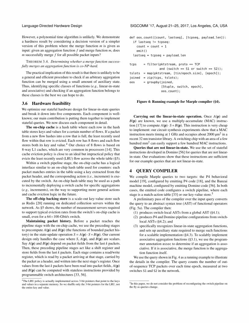
def oos_count([count, lastseq], [tcpseq, payload_len]):
if lastseq != tcpseq:
count = count + 1
emit()
lastseq = tcpseq + payload_len
tcps = filter(pktstream, proto == TCP
and (switch == S1 or switch == S2));
tslots = map(pktstream, [tin/epoch_size], [epoch]);
joined = zip(tcps, tslots);
oos = groupby(joined,
[5tuple, switch, epoch],
oos_count);
Figure 4: Running example for Marple compiler (§4).
Carrying out the linear-in-state operation. Once A(p) andB(p) are known, we use a multiply-accumulate (MAC) instruc-tion [17] to compute A(p) ·S+B(p). This instruction is very cheapto implement: our circuit synthesis experiments show that a MACinstruction meets timing at 1 GHz and occupies about 2000 µm2 in arecent 32 nm transistor library. A switching chip with an area of a fewhundred mm2 can easily support a few hundred MAC instructions.
Queries that are not linear-in-state. We use the set of statefulinstructions developed in Domino [56] for queries that are not linear-in-state. Our evaluations show that these instructions are sufficientfor our example queries that are not linear-in-state.
4 QUERY COMPILERWe compile Marple queries to two targets: the P4 behavioralmodel [19], configured by emitting P4 code [18], and the Banzaimachine model, configured by emitting Domino code [56]. In bothcases, the emitted code configures a switch pipeline, where eachstage is a match-action table [33] or our key-value store.5
A preliminary pass of the compiler over the input query convertsthe query to an abstract syntax tree (AST) of functional operators(Fig. 5a). The compiler then:
(1) produces switch-local ASTs from a global AST (§4.1);(2) produces P4 and Domino pipeline configurations from switch-
local ASTs (§4.2); and(3) specifically recognizes linear-in-state aggregation functions,
and sets up auxiliary state required to merge such functionsfor a scalable implementation (§4.3). To scalably implementassociative aggregation functions (§3.1), we use the program-mer annotation assoc to determine if an aggregation is asso-ciative. If it is associative, the merge function is the aggrega-tion function itself.
We use the query shown in Fig. 4 as a running example to illustratethe details in the compiler. The query counts the number of out-of-sequence TCP packets over each time epoch, measured at twoswitches S1 and S2 in the network.
5In this paper, we do not consider the problem of reconfiguring the switch pipeline onthe fly as queries change.
SIGCOMM ’17, August 21–25, 2017, Los Angeles, CA, USA S. Narayana et al.
filter
group
map
zip
Pktstream
Pktstream
S1,S2
S1,S2
all
S1,S2
all all
False
True
False
False
False False
(a) (b) (c)
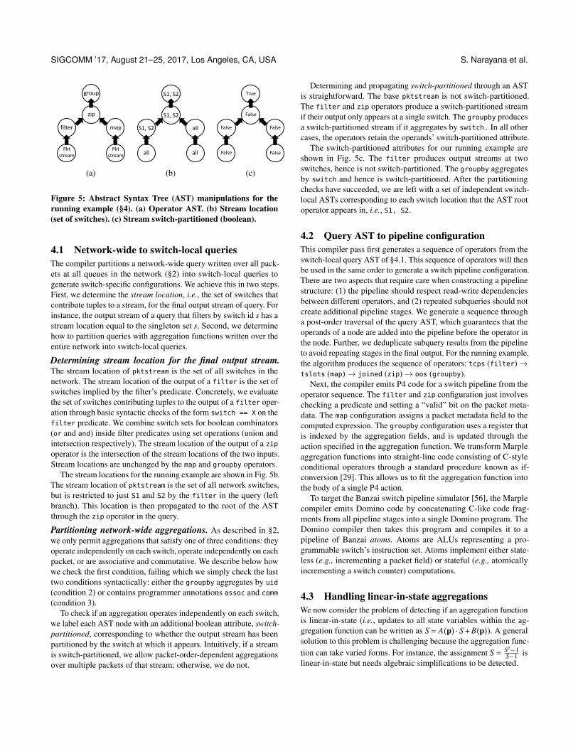
Figure 5: Abstract Syntax Tree (AST) manipulations for therunning example (§4). (a) Operator AST. (b) Stream location(set of switches). (c) Stream switch-partitioned (boolean).
4.1 Network-wide to switch-local queriesThe compiler partitions a network-wide query written over all pack-ets at all queues in the network (§2) into switch-local queries togenerate switch-specific configurations. We achieve this in two steps.First, we determine the stream location, i.e., the set of switches thatcontribute tuples to a stream, for the final output stream of query. Forinstance, the output stream of a query that filters by switch id s has astream location equal to the singleton set s. Second, we determinehow to partition queries with aggregation functions written over theentire network into switch-local queries.
Determining stream location for the final output stream.The stream location of pktstream is the set of all switches in thenetwork. The stream location of the output of a filter is the set ofswitches implied by the filter’s predicate. Concretely, we evaluatethe set of switches contributing tuples to the output of a filter oper-ation through basic syntactic checks of the form switch == X on thefilter predicate. We combine switch sets for boolean combinators(or and and) inside filter predicates using set operations (union andintersection respectively). The stream location of the output of a zip
operator is the intersection of the stream locations of the two inputs.Stream locations are unchanged by the map and groupby operators.
The stream locations for the running example are shown in Fig. 5b.The stream location of pktstream is the set of all network switches,but is restricted to just S1 and S2 by the filter in the query (leftbranch). This location is then propagated to the root of the ASTthrough the zip operator in the query.
Partitioning network-wide aggregations. As described in §2,we only permit aggregations that satisfy one of three conditions: theyoperate independently on each switch, operate independently on eachpacket, or are associative and commutative. We describe below howwe check the first condition, failing which we simply check the lasttwo conditions syntactically: either the groupby aggregates by uid
(condition 2) or contains programmer annotations assoc and comm
(condition 3).To check if an aggregation operates independently on each switch,
we label each AST node with an additional boolean attribute, switch-partitioned, corresponding to whether the output stream has beenpartitioned by the switch at which it appears. Intuitively, if a streamis switch-partitioned, we allow packet-order-dependent aggregationsover multiple packets of that stream; otherwise, we do not.
Determining and propagating switch-partitioned through an ASTis straightforward. The base pktstream is not switch-partitioned.The filter and zip operators produce a switch-partitioned streamif their output only appears at a single switch. The groupby producesa switch-partitioned stream if it aggregates by switch. In all othercases, the operators retain the operands’ switch-partitioned attribute.
The switch-partitioned attributes for our running example areshown in Fig. 5c. The filter produces output streams at twoswitches, hence is not switch-partitioned. The groupby aggregatesby switch and hence is switch-partitioned. After the partitioningchecks have succeeded, we are left with a set of independent switch-local ASTs corresponding to each switch location that the AST rootoperator appears in, i.e., S1, S2.
4.2 Query AST to pipeline configurationThis compiler pass first generates a sequence of operators from theswitch-local query AST of §4.1. This sequence of operators will thenbe used in the same order to generate a switch pipeline configuration.There are two aspects that require care when constructing a pipelinestructure: (1) the pipeline should respect read-write dependenciesbetween different operators, and (2) repeated subqueries should notcreate additional pipeline stages. We generate a sequence througha post-order traversal of the query AST, which guarantees that theoperands of a node are added into the pipeline before the operator inthe node. Further, we deduplicate subquery results from the pipelineto avoid repeating stages in the final output. For the running example,the algorithm produces the sequence of operators: tcps (filter)→tslots (map)→ joined (zip)→ oos (groupby).
Next, the compiler emits P4 code for a switch pipeline from theoperator sequence. The filter and zip configuration just involveschecking a predicate and setting a “valid” bit on the packet meta-data. The map configuration assigns a packet metadata field to thecomputed expression. The groupby configuration uses a register thatis indexed by the aggregation fields, and is updated through theaction specified in the aggregation function. We transform Marpleaggregation functions into straight-line code consisting of C-styleconditional operators through a standard procedure known as if-conversion [29]. This allows us to fit the aggregation function intothe body of a single P4 action.
To target the Banzai switch pipeline simulator [56], the Marplecompiler emits Domino code by concatenating C-like code frag-ments from all pipeline stages into a single Domino program. TheDomino compiler then takes this program and compiles it to apipeline of Banzai atoms. Atoms are ALUs representing a pro-grammable switch’s instruction set. Atoms implement either state-less (e.g., incrementing a packet field) or stateful (e.g., atomicallyincrementing a switch counter) computations.
4.3 Handling linear-in-state aggregationsWe now consider the problem of detecting if an aggregation functionis linear-in-state (i.e., updates to all state variables within the ag-gregation function can be written as S = A(p) ·S+B(p)). A generalsolution to this problem is challenging because the aggregation func-tion can take varied forms. For instance, the assignment S = S2−1
S−1 islinear-in-state but needs algebraic simplifications to be detected.
Language-Directed Hardware Design SIGCOMM ’17, August 21–25, 2017, Los Angeles, CA, USA
Step 1: Compute history for each state variable
Step 2: Are all state variable updates linear-in-state?(Finite history variables are trivially linear in state)
Query is scalableStep 3: Compute auxiliary state required for merge
Query is not scalable
YES
NO
Aggregation function code(in Marple)
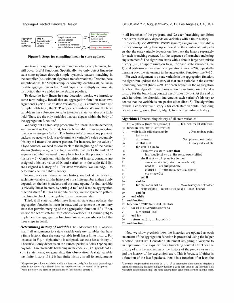
Figure 6: Steps for compiling linear-in-state updates.
We take a pragmatic approach and sacrifice completeness, butstill cover useful functions. Specifically, we only detect linear-in-state state updates through simple syntactic pattern matching inthe compiler (i.e., without algebraic transformations). Despite thesesimplifications, the Marple compiler correctly identifies all the linear-in-state aggregations in Fig. 7 and targets the multiply-accumulateinstruction that we added to the Banzai pipeline.
To describe how linear-in-state detection works, we introducesome terminology. Recall that an aggregation function takes twoarguments (§2): a list of state variables (e.g., a counter) and a listof tuple fields (e.g., the TCP sequence number). We use the termvariable in this subsection to refer to either a state variable or a tuplefield. These are the only variables that can appear within the body ofthe aggregation function.6
We carry out a three-step procedure for linear-in-state detection,summarized in Fig. 6. First, for each variable in an aggregationfunction we assign a history. This history tells us how many previouspackets we need to look at to determine a variable’s value accurately(history = 1 means the current packet). For instance, for the value ofa byte counter, we need to look back to the beginning of the packetstream (history = ∞), while for a variable that tracks the last TCPsequence number we need to only look back to the previous packet(history = 2). Consistent with the definition of history, constants areassigned a history value of 0, and variables in the tuple field listare assigned a history of 1. For state variables, we use Alg. 1 todetermine each variable’s history.
Second, once each variable has a history, we look at the history ofeach state variable s. If the history of s is a finite number k, then s onlydepends on the last k packets and the state update for that variableis trivially linear-in-state, by setting A to 0 and B to the aggregationfunction itself.7 If s has an infinite history, we use syntactic patternmatching to check if the update to s is linear-in-state.
Third, if all state variables have linear-in-state state updates, theaggregation function is linear-in-state, and we generate the auxiliarystate that permits merging of the aggregation function (§3). If not,we use the set of stateful instructions developed in Domino [56] toimplement the aggregation function. We now describe each of thethree steps in detail.
Determining history of variables. To understand Alg. 1, observethat if all assignments to a state variable only use variables that havea finite history, then the state variable itself has a finite history. Forinstance, in Fig. 4, right after it is assigned, lastseq has a history of1 because it only depends on the current packet’s fields tcpseq andpayload_len. To handle branching in the code, i.e., if (predicate)
{...} statements, we generalize this observation. A state variablehas finite history if (1) it has finite history in all its assignments
6Marple supports local variables within the function body, but the more general algo-rithm is not materially different from the simpler version we present in this paper.7More precisely, the parts of the aggregation function that update s.
in all branches of the program, and (2) each branching conditionpredicate itself only depends on variables with a finite history.
Concretely, COMPUTEHISTORY (line 2) assigns each variable ahistory corresponding to an upper bound on the number of past pack-ets that the state variable depends on. We track the history separatelyfor each branching context, i.e., the sequence of branches enclosingany statement.8 The algorithm starts with a default large pessimistichistory (i.e., an approximation to ∞) for each state variable (line1), and performs a fixed-point computation (lines 3–20), repeatedlyiterating over the statements in the aggregation function (line 7–16).
For each assignment to a state variable in the aggregation function,the algorithm updates the history of that state variable in the currentbranching context (lines 7–9). For each branch in the aggregationfunction, the algorithm maintains a new branching context and ahistory for the branching context itself (lines 10–14). At the end ofeach iteration, the algorithm increments each variable’s history todenote that the variable is one packet older (line 18). The algorithmreturns a conservative history k for each state variable, includingpossibly max_bound (line 1, Alg. 1) to reflect an infinite history.
Algorithm 1 Determining history of all state variables1: hist = {state = {true: max_bound}} ▷ Init. hist. for all state vars.2: function COMPUTEHISTORY(fun)3: while hist is still changing do ▷ Run to fixed point.4: hist← {}5: ctx← true ▷ Set up outermost context.6: ctxHist← 0 ▷ History value of ctx.7: for stmt in fun do8: if stmt == state = expr then9: hist[state][ctx]← GETHIST(ctx, expr, ctxHist)
10: else if stmt == if predicate then11: save context info (restore on branch exit)12: newCtx← ctx and predicate13: ctxHist← GETHIST(ctx, newCtx, ctxHist)14: ctx← newCtx15: end if16: end for17: for ctx, var in hist do ▷ Make history one pkt older.18: hist[var][ctx]← min(hist[var][ctx] + 1, max_bound)19: end for20: end while21: end function22: function GETHIST(ctx, ast, ctxHist)23: for xi ∈ LEAFNODES(ast) do24: hi = hist[xi][ctx]25: end for26: return max(h1, ... , hn, ctxHist)27: end function
Now we show precisely how the histories are updated as eachstatement of the aggregation function is processed using the helperfunction GETHIST. Consider a statement assigning a variable toan expression, x = expr, within a branching context ctx. Then thehistory of x is the maximum of the history of the predicates in ctx
and the history of the expression expr. This is because if either isa function of the last k packets, then x is a function of at least the8Currently, Marple forbids multiple if ... else statements at the same nesting level;hence, the enclosing branches uniquely identify a code path through the function. Thisrestriction is not fundamental; the more general form can be transformed into this form.
SIGCOMM ’17, August 21–25, 2017, Los Angeles, CA, USA S. Narayana et al.
last k packets. To determine the history of expr, suppose the ASTof expr contains the variables x1, x2, ..., xn as its leaves. Then,the history of expr is the maximum of the histories of the xi. Forexample, the history for lastseq after its assignment in oos_count
is the maximum of 1 (tcpseq and payload_len are functions of thecurrent packet), and 0 (for the enclosing outermost context true).
Determining if a state variable’s update is linear-in-state.For each state variable S with an infinite history, we check whetherthe state updates are linear-in-state as follows: (1) each update to Sis syntactically affine, i.e., S← A ·S+B with either A or B possiblyzero; and (2) A, B and every branch predicate depend on variableswith a finite history. This approach is sound, but incomplete: itmisses updates such as S = S2−1
S−1 .
Determining auxiliary state. For each state variable with a linear-in-state update, we initialize four pieces of auxiliary state for a newlyinserted key:9 (1) a running product SA = 1; (2) a packet counterc = 0; (3) an entry log, consisting of relevant fields from the first kpackets following insertion; and (4) an exit log, consisting of relevantfields from the last k packets seen so far. After the counter c crossesthe packet history bound k, we update SA to A · SA each time S isupdated.10 When the key is evicted, we send SA along with the entryand exit logs to the backing store for merging (details are in ourtechnical report [15]).
5 EVALUATIONWe evaluate Marple in three ways. In §5.1, we quantify the hard-ware resources required for Marple queries. In §5.2, we measurethe memory-eviction tradeoff for the key-value store. In §5.3 and§5.4, we show two case studies that use Marple compiled to the P4behavioral model running on Mininet: debugging microbursts [44]and computing flowlet size distributions.
5.1 Hardware compute resourcesFig. 7 shows several Marple queries. Alongside each query, we show(1) whether all its aggregations are linear-in-state, (2) whether itcan be scaled by merging correctly with a backing store, and (3)the switch resources required, measured through the pipeline depth(number of stages), width (maximum number of parallel compu-tations per stage), and number of Banzai atoms (total number ofcomputations) required.
Fig. 7 shows that many useful queries contain only linear-in-stateaggregations, and most of them scale to a large number of keys (§3.2).Notably, the flowlet size histogram and lossy connection queries arenot scalable despite being linear-in-state, since they contain emit()
statements. In §3.4, we showed how to rewrite some of these queries(e.g., lossy connections) to scale, at the cost of losing some accuracy.
We compute the pipeline’s depth and width by compiling eachquery to the Banzai switch pipeline simulator. Banzai is suppliedwith stateless atoms, which perform binary operations (arithmetic,logic, and relational) on pairs of packet fields, and one stateful atom.For the linear-in-state operations, we use the multiply-accumulateatom as the stateful atom, while for the other operations, we useBanzai’s own NestedIf atom [56]. The Domino compiler determines
9This can happen either when a key first appears or reappears following an eviction.10This stateful update itself can be implemented through a multiply-accumulate atom.
whether the input program can be mapped to a pipeline with thespecified atoms. As expected, all the linear-in-state queries map to apipeline with the multiply-accumulate atom.
The computational resources required for Marple queries aremodest. All queries in Fig. 7 require a pipeline shorter than 11 stages.This is feasible, e.g., the RMT architecture offers 32 stages [33].Further, functionality other than measurement can run in parallelbecause the number of atoms required per stage is at most 6, whileprogrammable switches provide ~100 parallel instructions per stage(e.g., RMT provides 224 [33]).
5.2 Memory and bandwidth overheadsIn this section, we answer the following questions:
(1) What is a good size for the on-chip key value store?(2) What are the eviction rates to the backing store?(3) How accurate are queries that are not mergeable?
Experimental setup. We simulate a Marple query over three un-sampled packet traces: two traces from 10 Gbit/s core Internetrouters, one from Chicago (~150M packets) from 2016 [24] andone from San Jose (~189M packets) from 2014 [23]; and a 2.5 houruniversity data-center trace (~100M packets) from 2010 [32]. Werefer to these traces as Core16, Core14, and DC respectively.
We evaluate the impact of memory size on cache evictions fora Marple query that aggregates by 5-tuple. As discussed in §3.6,our hardware design uses an 8-way LRU cache. We also evaluatetwo other geometries: a hash table, which evicts the incumbent keyupon a collision, and a fully associative LRU. Comparing our 8-wayLRU with other hardware designs demonstrates the tradeoff betweenhardware complexity and eviction rate.
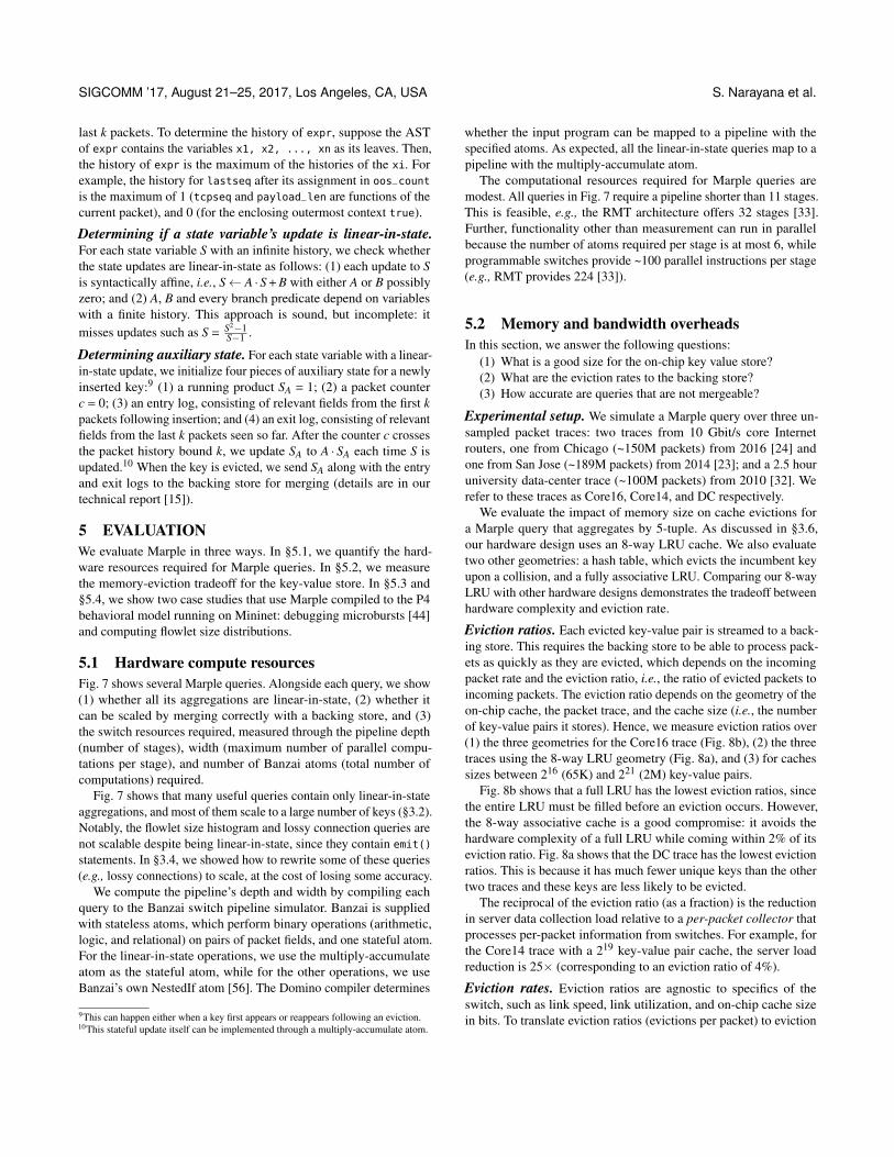
Eviction ratios. Each evicted key-value pair is streamed to a back-ing store. This requires the backing store to be able to process pack-ets as quickly as they are evicted, which depends on the incomingpacket rate and the eviction ratio, i.e., the ratio of evicted packets toincoming packets. The eviction ratio depends on the geometry of theon-chip cache, the packet trace, and the cache size (i.e., the numberof key-value pairs it stores). Hence, we measure eviction ratios over(1) the three geometries for the Core16 trace (Fig. 8b), (2) the threetraces using the 8-way LRU geometry (Fig. 8a), and (3) for cachessizes between 216 (65K) and 221 (2M) key-value pairs.
Fig. 8b shows that a full LRU has the lowest eviction ratios, sincethe entire LRU must be filled before an eviction occurs. However,the 8-way associative cache is a good compromise: it avoids thehardware complexity of a full LRU while coming within 2% of itseviction ratio. Fig. 8a shows that the DC trace has the lowest evictionratios. This is because it has much fewer unique keys than the othertwo traces and these keys are less likely to be evicted.
The reciprocal of the eviction ratio (as a fraction) is the reductionin server data collection load relative to a per-packet collector thatprocesses per-packet information from switches. For example, forthe Core14 trace with a 219 key-value pair cache, the server loadreduction is 25× (corresponding to an eviction ratio of 4%).
Eviction rates. Eviction ratios are agnostic to specifics of theswitch, such as link speed, link utilization, and on-chip cache sizein bits. To translate eviction ratios (evictions per packet) to eviction
Language-Directed Hardware Design SIGCOMM ’17, August 21–25, 2017, Los Angeles, CA, USA
Example Query code Description Linear Scales? Pipe Pipe # ofin state? depth width atoms
Packet counts def count([cnt], []): cnt = cnt + 1; emit() Count packets per source IP. Yes Yes 5 2 7result = groupby(pktstream, [srcip], count);
EWMA over latencies def ewma([avg], [tin, tout]): Maintain a moving EWMA over Yes Yes 6 4 11avg = (1-alpha)*avg + (alpha)*(tout-tin) packet latencies per flow.
ewma_q = groupby(pktstream, [5tuple], ewma);
TCP out-of-sequence def oos([lastseq, cnt], [tcpseq, payload_len]): Count the number of packets per Yes Yes 7 4 14if lastseq != tcpseq: cnt = cnt + 1 connection arriving with a sequencelastseq = tcpseq + payload_len number that is non-consecutive with
oos_q = groupby(pktstream, [5tuple], oos); the last packet.TCP non-monotonic def nonmt([maxseq, cnt], [tcpseq]): Count the number of packets per No No 5 2 6
if maxseq > tcpseq: cnt = cnt + 1 connection with sequence numberselse: maxseq = tcpseq lower than the maximum so far.
nm_q = groupby(pktstream, [5tuple], nonmt);
Flowlet size def fl_detect([last_time, size], [tin]): Compute a histogram over the Yes No 11 6 31histogram if tin - last_time > delta: lengths of flowlets. This statistic is
emit(); size = 1 useful to evaluate network loadelse: size = size + 1 balancing schemes, e.g., [27].last_time = tin
R1 = groupby(pktstream, [5tuple], fl_detect);
fl_hist = groupby(R1, [size], count);
High E2E latency def sum_lat([e2e_lat], [tin, tout]): Capture packets experiencing high Yes Yes 5 3 8e2e_lat = e2e_lat + tout - tin end-to-end queueing latency, by
e2e = groupby(pktstream, [uid], sum_lat); adding time spent in the queue athigh_e2e = filter(e2e, e2e_lat > 10); each hop.
Count concurrently def new_flow([cnt], []): Count the number of active No No 4 3 10active connections if cnt == 0: emit(); cnt = 1 connections in a queue over a
R1 = map(pktstream, [tin/128], [epoch]); period of time (“epoch”).R2 = groupby(R1, [5tuple, epoch], new_flow);
num_conns = groupby(R2, [epoch], count);
TCP incast R3 = zip(num_conns, pktstream); Detect when many connections use No No 7 4 14ic_q = filter(R3, qin > 100 and cnt < 25); a long queue. Uses the query above.
Lossy connections total = groupby(pktstream, [5tuple], count); Compute packet loss rate per Yes No 8 4 19R1 = filter(pktstream, tout == infinity); connection, reporting connectionslost = groupby(R1, [5tuple], count); with packet drop rate higher thanZ = zip(total, lost); a threshold p.
lc_q = filter(Z, lost.cnt > p*total.cnt);
TCP timeouts def timeout([cnt], [last_time, tin]): Count the number of timeouts for Yes Yes 8 3 15timediff = tin - last_time each TCP connection, by checkingif timediff > 280ms and timediff < 320ms: for packet inter-arrival times
cnt = cnt + 1 around 300 ms (retransmissionlast_time = tin timer).
to_q = groupby(pktstream, [5tuple], timeout);
Figure 7: Examples of performance queries. We report that a query scales to a large number of keys either if (1) there are no statefulupdates involved, or (2) all its stateful updates are linear-in-state and there are no emit()s. We use Domino [56] to report the hardwareresources, i.e., atom count and pipeline depth and width. Linear-in-state queries use the multiply-accumulate atom (§3); others use aNestedIf atom [56] that supports updates predicated on the state value itself.
0 2 4 6 8
10 12
16 17 18 19 20 21
% E
vict
ed
log_2(Cache Slots)
Core16Core14
DC
(a) By trace
0 2 4 6 8
10 12
16 17 18 19 20 21
% E
vict
ed
log_2(Cache Slots)
Hash Table8-way associative
Full LRU
(b) By cache geometry (Core16)Figure 8: Eviction ratios to the backing store.
rates (evictions per second), we first compute the average packetsize (700 Bytes) and link utilization (30%) from the Core16 trace.
Next, we estimate the on-chip cache size for a 64×10-Gbit/sswitch and a 64×100-Gbit/s switch. On a 64×10-Gbit/s switch,SRAM densities are ≈ 3–4 Mbit/mm2 [1], and the smallest switch-ing chips occupy 200 mm2 [39]. Therefore, a 64 Mbit cache in
SRAM costs around 10% additional area, which we believe is rea-sonable. For recent 64×100-Gbit/s switches [5], SRAM densities are≈ 7Mbit/mm2 [22], and the switches occupy ≈ 500 mm2,11 making a256 Mbit cache (7.3% area overhead) a reasonable target.
For a given query, we divide these cache sizes by the size of theaggregation’s key-value pair to get the number of key-value pairs.We then look up this number in Fig. 8 to get the eviction ratio forthat query, which we translate to an eviction rate using the networkutilization and packet size mentioned earlier.
Eviction rates for some sample queries are shown in Fig. 9. Fora 64×10-Gbit/s switch with a 64 Mbit cache, we observe evictionrates of ≈ 1M packets per second. For a 64×100-Gbit/s switch witha 256 Mbit cache and the same average packet size and utilization,
11S. Chole. Cisco Systems. Private communication. June 2017.
SIGCOMM ’17, August 21–25, 2017, Los Angeles, CA, USA S. Narayana et al.
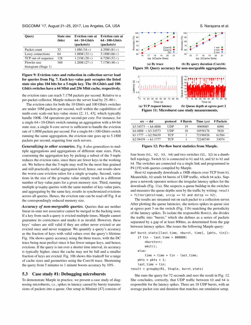
Query State size Eviction rate at Eviction rate at(bits) 64×10-Gbit/s 64×100-Gbit/s
(packets/s) (packets/s)Packet count 32 1.0M (34×) 4.29M (81×)Lossy connections 64 1.08M (32×) 5.18M (66×)TCP out-of-sequence 128 1.21M (28×) 6.72M (52×)Flowlet size 160 1.26M (27×) 7.17M (48×)histogram (Stage 1)
Figure 9: Eviction rates and reduction in collection server loadfor queries from Fig. 7. Each key-value pair occupies the listedstate size plus 104 bits for a 5-tuple key. The 10-Gbit/s and 100-Gbit/s switches have a 64 Mbit and 256 Mbit cache, respectively.
the eviction rates can reach 7.17M packets per second. Relative to aper-packet collector, Marple reduces the server load by 25–80×.
The eviction rates for both the 10 Gbit/s and 100 Gbit/s switchesare under 10M packets per second, well within the capabilities ofmulti-core scale-out key-value stores [2, 11, 43], which typicallyhandle 100K–1M operations per second per core. For instance, fora single 64×10-Gbit/s switch running an aggregation with a 64-bitstate size, a single 8-core server is sufficient to handle the evictionrate of 1.08M packets per second. For a single 64×100-Gbit/s switchrunning the same aggregation, the eviction rate goes up to 5.18Mpackets per second, requiring four such servers.
Generalizing to other scenarios. Fig. 8 also generalizes to mul-tiple aggregations and aggregations of different state sizes. First,coarsening the aggregation key by picking a subset of the 5-tuplereduces the eviction ratio, since there are fewer keys in the workingset. We believe that the 5-tuple may well be the most fine-grainedand still practically useful aggregation level; hence, our results showthe worst-case eviction ratios for a single groupby. Second, varia-tions in the size of the groupby value simply result in a differentnumber of key-value pairs for a given memory size. Third, runningmultiple groupby queries with the same number of key-value pairs,and aggregating by the same key, results in synchronized evictionsacross all queries. Hence, the eviction rate can be read off Fig. 8 atthe correspondingly reduced memory size.
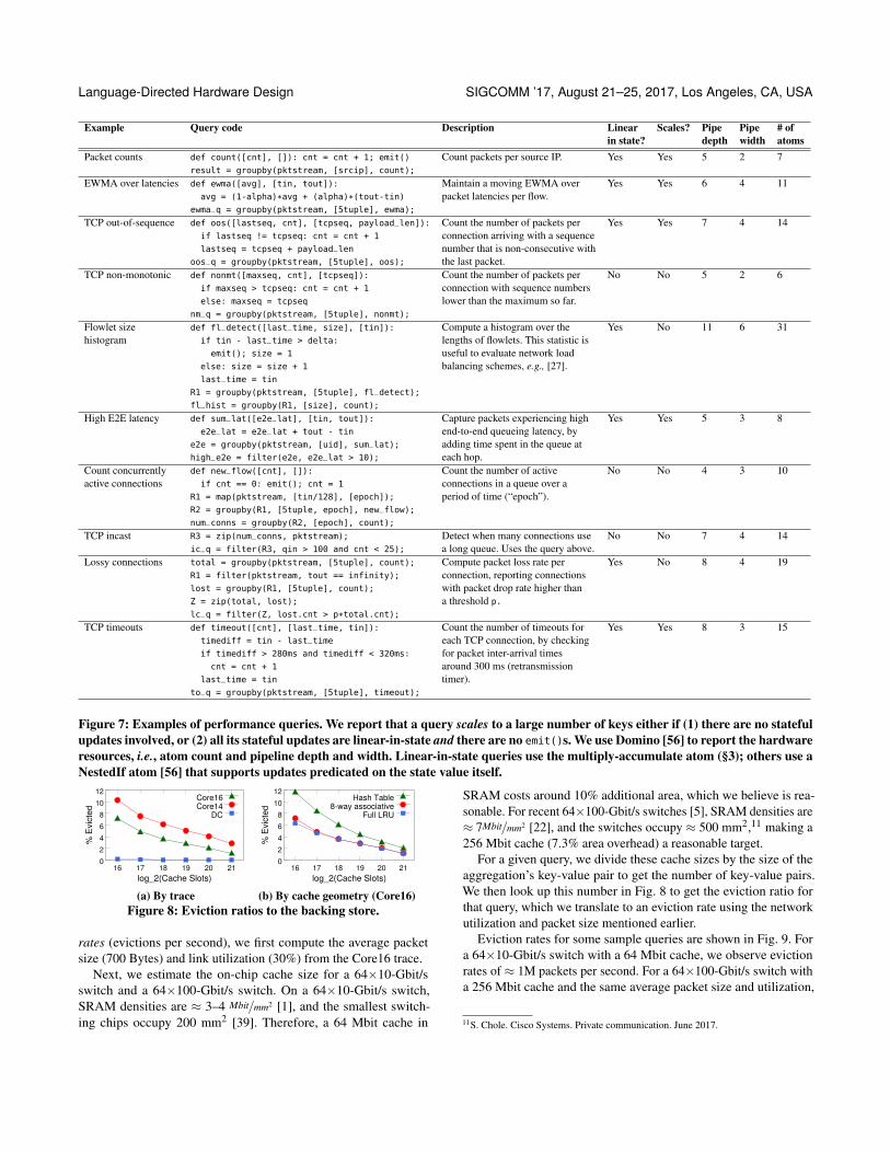
Accuracy of non-mergeable queries. Queries that are neitherlinear-in-state nor associative cannot be merged in the backing store.If a key from such a query is evicted multiple times, Marple cannotguarantee its correctness and marks it as invalid. However, thesekeys’ values are still valid if they are either never evicted or areevicted once and never reappear. We quantify a query’s accuracyas the fraction of keys with valid values over the query’s lifetime.Fig. 10a shows query accuracy using the three traces, with the DCtrace being near-perfect since it has fewer unique keys, and hence,evictions. If the query is run over a shorter time interval, its accuracyis typically higher, since the cache may not be full and a smallerfraction of keys are evicted. Fig. 10b shows this tradeoff for a rangeof cache sizes and geometries using the Core16 trace. Shorteningthe query from 5 minutes to 1 minute boosts accuracy by 10%.
5.3 Case study #1: Debugging microburstsTo demonstrate Marple in practice, we present a case study of diag-nosing microbursts, i.e., spikes in latency caused by bursty transmis-sions of packets into a queue. Our setup in Mininet [47] consists of
50
60
70
80
90
100
16 17 18 19 20 21
Accu
racy
(%)
log_2(Cache Slots)
Core16Core14
DC
(a) By trace
50
60
70
80
90
100
16 17 18 19 20 21
Accu
racy
(%)
log_2(Cache Slots)
1 min3 min5 min
(b) By query duration (Core16)Figure 10: Query accuracy for non-mergeable aggregations.
0
0.5
1
1.5
2
0 10 20 30 40 50 60 70 80 90
Late
ncy
(s)
Time (s)(a) TCP request latency
0 10 20 30 40 50 60 70
0 10 20 30 40 50 60 70 80 90
Que
ue (#
pac
kets
)
Time (s)(b) Queue depth at egress port 2
Figure 11: Microburst case study measurements.
src→ dst protocol # Bursts Time (µs) # Packetsh3:34573→ h4:4888 UDP 19 8969085 6090h4:4888→ h3:34573 UDP 18 10558176 5820h1:1777→ h2:58439 TCP 1 72196926 61584h2:58439→ h1:1777 TCP 1 72248749 33074
Figure 12: Per-flow burst statistics from Marple.
four hosts (h1, h2, h3, h4) and two switches (S1, S2) in a dumb-bell topology. Switch S1 is connected to h1 and h3, and S2 to h2 andh4. The switches are connected via a single link and programmed inP4 [19] with queries compiled by Marple.
Host h2 repeatedly downloads a 1MB objects over TCP from h1.Meanwhile, h3 sends h4 bursts of UDP traffic, which h4 acks. Sup-pose a network operator notices the irregular latency spikes for thedownloads (Fig. 11a). She suspects a queue buildup in the switchesand measures the queue depths seen by the traffic by writing: result= filter(pktstream, srcip == h1 and dstip == h2).
The results are streamed out on each packet to a collection server.After plotting the queue latencies, she notices spikes in queue sizeat egress port 3 on the switch (Fig. 11b) matching the periodicityof the latency spikes. To isolate the responsible flow(s), she dividesthe traffic into “bursts,” which she defines as a series of packetsseparated by a gap of at least 800ms, as determined from the gapbetween latency spikes. She issues the following Marple query:
def burst_stats([last_time, nburst, time], [pkts, tin]):
if tin - last_time > 800000:
nbursts++;
emit();
else:
time = time + tin - last_time;
pkts = pkts + 1;
last_time = tin;
result = groupby(R1, 5tuple, burst_stats)
She runs the query for 72 seconds and sees the result in Fig. 12.She concludes, correctly, that UDP traffic between h3 and h4 isresponsible for the latency spikes. There are 18 UDP bursts, with anaverage packet size and duration that matches our emulation setup.
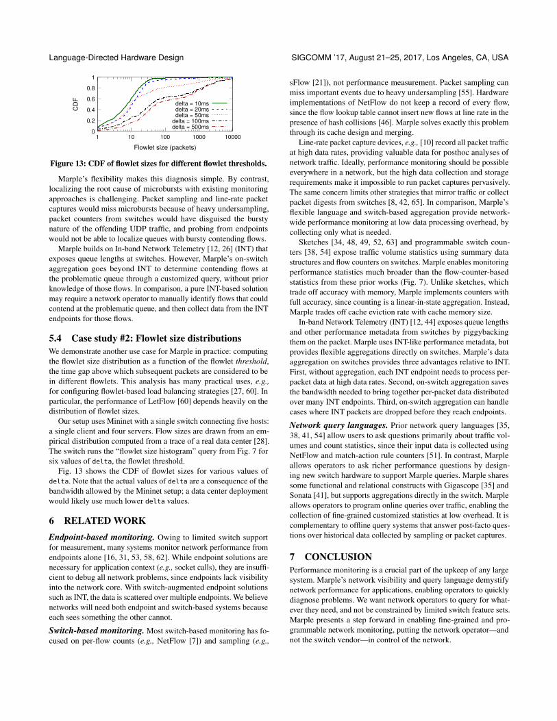
Language-Directed Hardware Design SIGCOMM ’17, August 21–25, 2017, Los Angeles, CA, USA
0
0.2
0.4
0.6
0.8
1
1 10 100 1000 10000
CD
F
Flowlet size (packets)
delta = 10msdelta = 20msdelta = 50ms
delta = 100msdelta = 500ms
Figure 13: CDF of flowlet sizes for different flowlet thresholds.
Marple’s flexibility makes this diagnosis simple. By contrast,localizing the root cause of microbursts with existing monitoringapproaches is challenging. Packet sampling and line-rate packetcaptures would miss microbursts because of heavy undersampling,packet counters from switches would have disguised the burstynature of the offending UDP traffic, and probing from endpointswould not be able to localize queues with bursty contending flows.
Marple builds on In-band Network Telemetry [12, 26] (INT) thatexposes queue lengths at switches. However, Marple’s on-switchaggregation goes beyond INT to determine contending flows atthe problematic queue through a customized query, without priorknowledge of those flows. In comparison, a pure INT-based solutionmay require a network operator to manually identify flows that couldcontend at the problematic queue, and then collect data from the INTendpoints for those flows.
5.4 Case study #2: Flowlet size distributionsWe demonstrate another use case for Marple in practice: computingthe flowlet size distribution as a function of the flowlet threshold,the time gap above which subsequent packets are considered to bein different flowlets. This analysis has many practical uses, e.g.,for configuring flowlet-based load balancing strategies [27, 60]. Inparticular, the performance of LetFlow [60] depends heavily on thedistribution of flowlet sizes.
Our setup uses Mininet with a single switch connecting five hosts:a single client and four servers. Flow sizes are drawn from an em-pirical distribution computed from a trace of a real data center [28].The switch runs the “flowlet size histogram” query from Fig. 7 forsix values of delta, the flowlet threshold.
Fig. 13 shows the CDF of flowlet sizes for various values ofdelta. Note that the actual values of delta are a consequence of thebandwidth allowed by the Mininet setup; a data center deploymentwould likely use much lower delta values.
6 RELATED WORKEndpoint-based monitoring. Owing to limited switch supportfor measurement, many systems monitor network performance fromendpoints alone [16, 31, 53, 58, 62]. While endpoint solutions arenecessary for application context (e.g., socket calls), they are insuffi-cient to debug all network problems, since endpoints lack visibilityinto the network core. With switch-augmented endpoint solutionssuch as INT, the data is scattered over multiple endpoints. We believenetworks will need both endpoint and switch-based systems becauseeach sees something the other cannot.
Switch-based monitoring. Most switch-based monitoring has fo-cused on per-flow counts (e.g., NetFlow [7]) and sampling (e.g.,
sFlow [21]), not performance measurement. Packet sampling canmiss important events due to heavy undersampling [55]. Hardwareimplementations of NetFlow do not keep a record of every flow,since the flow lookup table cannot insert new flows at line rate in thepresence of hash collisions [46]. Marple solves exactly this problemthrough its cache design and merging.
Line-rate packet capture devices, e.g., [10] record all packet trafficat high data rates, providing valuable data for posthoc analyses ofnetwork traffic. Ideally, performance monitoring should be possibleeverywhere in a network, but the high data collection and storagerequirements make it impossible to run packet captures pervasively.The same concern limits other strategies that mirror traffic or collectpacket digests from switches [8, 42, 65]. In comparison, Marple’sflexible language and switch-based aggregation provide network-wide performance monitoring at low data processing overhead, bycollecting only what is needed.
Sketches [34, 48, 49, 52, 63] and programmable switch coun-ters [38, 54] expose traffic volume statistics using summary datastructures and flow counters on switches. Marple enables monitoringperformance statistics much broader than the flow-counter-basedstatistics from these prior works (Fig. 7). Unlike sketches, whichtrade off accuracy with memory, Marple implements counters withfull accuracy, since counting is a linear-in-state aggregation. Instead,Marple trades off cache eviction rate with cache memory size.
In-band Network Telemetry (INT) [12, 44] exposes queue lengthsand other performance metadata from switches by piggybackingthem on the packet. Marple uses INT-like performance metadata, butprovides flexible aggregations directly on switches. Marple’s dataaggregation on switches provides three advantages relative to INT.First, without aggregation, each INT endpoint needs to process per-packet data at high data rates. Second, on-switch aggregation savesthe bandwidth needed to bring together per-packet data distributedover many INT endpoints. Third, on-switch aggregation can handlecases where INT packets are dropped before they reach endpoints.
Network query languages. Prior network query languages [35,38, 41, 54] allow users to ask questions primarily about traffic vol-umes and count statistics, since their input data is collected usingNetFlow and match-action rule counters [51]. In contrast, Marpleallows operators to ask richer performance questions by design-ing new switch hardware to support Marple queries. Marple sharessome functional and relational constructs with Gigascope [35] andSonata [41], but supports aggregations directly in the switch. Marpleallows operators to program online queries over traffic, enabling thecollection of fine-grained customized statistics at low overhead. It iscomplementary to offline query systems that answer post-facto ques-tions over historical data collected by sampling or packet captures.
7 CONCLUSIONPerformance monitoring is a crucial part of the upkeep of any largesystem. Marple’s network visibility and query language demystifynetwork performance for applications, enabling operators to quicklydiagnose problems. We want network operators to query for what-ever they need, and not be constrained by limited switch feature sets.Marple presents a step forward in enabling fine-grained and pro-grammable network monitoring, putting the network operator—andnot the switch vendor—in control of the network.
SIGCOMM ’17, August 21–25, 2017, Los Angeles, CA, USA S. Narayana et al.
Acknowledgments. This work was supported by NSF grants CNS-1563826, CNS-1526791, and CNS-1617702, DARPA I2O Award No.HR0011-15-2-0047, and a gift from the Cisco Research Center. Wethank Jennifer Rexford, Fadel Adib, Amy Ousterhout, our shepherdMarco Canini, and the anonymous SIGCOMM reviewers for theirthoughtful feedback.
REFERENCES[1] 45 nanometer - Wikipedia, Technology demos. https://en.wikipedia.org/wiki/45_
nanometer#Technology_demos.[2] An Update on the Memcached/Redis Benchmark. http://oldblog.antirez.com/post/
update-on-memcached-redis-benchmark.html.[3] Barefoot: The World’s Fastest and Most Programmable Networks.
https://barefootnetworks.com/media/white_papers/Barefoot-Worlds-Fastest-Most-Programmable-Networks.pdf.
[4] Benchmarking Apache Kafka: 2 Million Writes Per Second (On Three CheapMachines). https://engineering.linkedin.com/kafka/benchmarking-apache-kafka-2-million-writes-second-three-cheap-machines.
[5] Broadcom First to Deliver 64 Ports of 100GE with Tomahawk II 6.4Tbps EthernetSwitch. https://www.broadcom.com/news/product-releases/broadcom-first-to-deliver-64-ports-of-100ge-with-tomahawk-ii-ethernet-switch.
[6] Cavium XPliant Switches and Microsoft Azure Networking Achieve SAI RoutingInteroperability. http://www.cavium.com/newsevents-Cavium-XPliant-Switches-and-Microsoft-Azure-Networking-Achieve -SAI-Routing-Interoperability.html.
[7] Cisco IOS NetFlow. http://www.cisco.com/c/en/us/products/ios-nx-os-software/ios-netflow/index.html.
[8] Configuring SPAN. http://www.cisco.com/c/en/us/td/docs/switches/lan/catalyst2940/software/release/12-1_19_ea1/configuration/guide/2940scg_1/swspan.html.
[9] Data center flow telemetry. http://www.cisco.com/c/en/us/products/collateral/data-center-analytics/tetration-analytics/white-paper-c11-737366.html.
[10] Gigamon. https://www.gigamon.com/products/visibility-nodes/visibility-appliances.html.
[11] How Fast is Redis? http://redis.io/topics/benchmarks.[12] In-band Network Telemetry. https://github.com/p4lang/p4factory/tree/master/
apps/int.[13] Intel FlexPipe. http://www.intel.com/content/dam/www/public/us/en/documents/
product-briefs/ethernet-switch-fm6000-series-brief.pdf.[14] Intel64 and IA-32 Architectures Optimization Reference Manual.
http://www.intel.com/content/dam/www/public/us/en/documents/manuals/64-ia-32-architectures-optimization-manual.pdf.
[15] Marple proofs. http://web.mit.edu/marple/marple_tr.pdf.[16] Microsoft bets big on SDN. https://azure.microsoft.com/en-us/blog/microsoft-
showcases-software-defined-networking-innovation-at-sigcomm-v2/.[17] Multiply-accumulate operation. https://en.wikipedia.org/wiki/Multiply-
accumulate_operation.[18] P4-16 Language Specification. http://p4.org/wp-content/uploads/2016/12/P4_16-
prerelease-Dec_16.html.[19] P4 Behavioral Model. https://github.com/p4lang/behavioral-model.[20] Redis. http://redis.io/.[21] sFlow. https://en.wikipedia.org/wiki/SFlow.[22] SRAM - ARM. https://www.arm.com/products/physical-ip/embedded-memory-
ip/sram.php.[23] The CAIDA UCSD Anonymized Internet Traces 2014 - June. http://www.caida.
org/data/passive/passive_2014_dataset.xml.[24] The CAIDA UCSD Anonymized Internet Traces 2016 - April. http://www.caida.
org/data/passive/passive_2016_dataset.xml.[25] XPliant™ Ethernet Switch Product Family. http://www.cavium.com/XPliant-
Ethernet-Switch-Product-Family.html.[26] The Future of Network Monitoring with Barefoot Networks. https://youtu.be/
Gbm7kDHXR-o, 2017.[27] M. Alizadeh, T. Edsall, S. Dharmapurikar, R. Vaidyanathan, K. Chu, A. Fingerhut,
V. T. Lam, F. Matus, R. Pan, N. Yadav, and G. Varghese. CONGA: DistributedCongestion-Aware Load Balancing for Datacenters. In SIGCOMM, 2014.
[28] Alizadeh, Mohammad. Empirical Traffic Generator. https://github.com/datacenter/empirical-traffic-gen, 2017.
[29] J. R. Allen, K. Kennedy, C. Porterfield, and J. Warren. Conversion of ControlDependence to Data Dependence. In POPL, 1983.
[30] A. Arasu, S. Babu, and J. Widom. The CQL Continuous Query Language: Seman-tic Foundations and Query Execution. The VLDB Journal, 2006.
[31] B. Arzani, S. Ciraci, B. T. Loo, A. Schuster, and G. Outhred. Taking the BlameGame out of Data Centers Operations with NetPoirot. In Proceedings of the 2016Conference on ACM SIGCOMM 2016 Conference, SIGCOMM ’16, 2016.
[32] T. Benson, A. Akella, and D. A. Maltz. Network Traffic Characteristics of DataCenters in the Wild. ACM International Measurement Conference, Nov. 2010.
[33] P. Bosshart, G. Gibb, H.-S. Kim, G. Varghese, N. McKeown, M. Izzard, F. Mujica,and M. Horowitz. Forwarding Metamorphosis: Fast Programmable Match-ActionProcessing in Hardware for SDN. In SIGCOMM, 2013.
[34] G. Cormode and S. Muthukrishnan. An Improved Data Stream Summary: TheCount-Min Sketch and Its Applications. Journal of Algorithms, 2005.
[35] C. Cranor, T. Johnson, O. Spataschek, and V. Shkapenyuk. Gigascope: A StreamDatabase for Network Applications. In SIGMOD, 2003.
[36] D. R. Ditzel and D. A. Patterson. Retrospective on High-level Language ComputerArchitecture. In ISCA, 1980.
[37] M. Dobrescu, K. Argyraki, and S. Ratnasamy. Toward Predictable Performance inSoftware Packet-processing Platforms. In NSDI, 2012.
[38] N. Foster, R. Harrison, M. J. Freedman, C. Monsanto, J. Rexford, A. Story, andD. Walker. Frenetic: A Network Programming Language. In ICFP, 2011.
[39] G. Gibb, G. Varghese, M. Horowitz, and N. McKeown. Design Principles forPacket Parsers. In ANCS, 2013.
[40] C. Guo, L. Yuan, D. Xiang, Y. Dang, R. Huang, D. Maltz, Z. Liu, V. Wang, B. Pang,H. Chen, Z.-W. Lin, and V. Kurien. Pingmesh: A Large-Scale System for DataCenter Network Latency Measurement and Analysis. In SIGCOMM, 2015.
[41] A. Gupta, R. Birkner, M. Canini, N. Feamster, C. Mac-Stoker, and W. Willinger.Network Monitoring is a Streaming Analytics Problem. In HOTNETS, 2016.
[42] N. Handigol, B. Heller, V. Jeyakumar, D. Mazières, and N. McKeown. I KnowWhat Your Packet Did Last Hop: Using Packet Histories to Troubleshoot Networks.In NSDI, 2014.
[43] S. Hart, E. Frachtenberg, and M. Berezecki. Predicting Memcached ThroughputUsing Simulation and Modeling. In Symposium on Theory of Modeling andSimulation, 2012.
[44] V. Jeyakumar, M. Alizadeh, Y. Geng, C. Kim, and D. Mazières. Millions of LittleMinions: Using Packets for Low Latency Network Programming and Visibility.In SIGCOMM, 2014.
[45] S. P. Jones and P. Wadler. Comprehensive Comprehensions. In Proceedings of theACM SIGPLAN Workshop on Haskell Workshop, 2007.
[46] M. Kumar and K. Prasad. Auto-learning of MAC addresses and lexicographiclookup of hardware database. US Patent App. 10/747,332.
[47] B. Lantz, B. Heller, and N. McKeown. A Network in a Laptop: Rapid Prototypingfor Software-defined Networks. In HotNets, 2010.
[48] Y. Li, R. Miao, C. Kim, and M. Yu. FlowRadar: A Better NetFlow for DataCenters. In NSDI, 2016.
[49] Z. Liu, A. Manousis, G. Vorsanger, V. Sekar, and V. Braverman. One Sketchto Rule Them All: Rethinking Network Flow Monitoring with UnivMon. InSIGCOMM, 2016.
[50] W. M. McKeeman. Language directed computer design. In Proceedings of theNovember 14-16, 1967, fall joint computer conference, 1967.
[51] N. McKeown, T. Anderson, H. Balakrishnan, G. Parulkar, L. Peterson, J. Rexford,S. Shenker, and J. Turner. OpenFlow: Enabling Innovation in Campus Networks.SIGCOMM Comput. Commun. Rev., 38(2):69–74, Mar. 2008.
[52] M. Moshref, M. Yu, R. Govindan, and A. Vahdat. DREAM: Dynamic ResourceAllocation for Software-defined Measurement. In SIGCOMM, 2014.
[53] M. Moshref, M. Yu, R. Govindan, and A. Vahdat. Trumpet: Timely and PreciseTriggers in Data Centers. In SIGCOMM, 2016.
[54] S. Narayana, M. Tahmasbi, J. Rexford, and D. Walker. Compiling Path Queries.In NSDI, 2016.
[55] P. Phaal. SFlow sampling rates, 2016. http://blog.sflow.com/2009/06/sampling-rates.html.
[56] A. Sivaraman, A. Cheung, M. Budiu, C. Kim, M. Alizadeh, H. Balakrishnan,G. Varghese, N. McKeown, and S. Licking. Packet Transactions: High-LevelProgramming for Line-Rate Switches. In SIGCOMM, 2016.
[57] A. Sivaraman, S. Subramanian, M. Alizadeh, S. Chole, S.-T. Chuang, A. Agrawal,H. Balakrishnan, T. Edsall, S. Katti, and N. McKeown. Programmable PacketScheduling at Line Rate. In SIGCOMM, 2016.
[58] P. Tammana, R. Agarwal, and M. Lee. Simplifying Datacenter Network Debuggingwith PathDump. In OSDI, 2016.
[59] D. Ungar, R. Blau, P. Foley, D. Samples, and D. Patterson. Architecture of SOAR:Smalltalk on a RISC. In ISCA, 1984.
[60] E. Vanini, R. Pan, M. Alizadeh, P. Taheri, and T. Edsall. Let it Flow: ResilientAsymmetric Load Balancing with Flowlet Switching. In NSDI, 2017.
[61] V. Vasudevan, A. Phanishayee, H. Shah, E. Krevat, D. G. Andersen, G. R. Ganger,G. A. Gibson, and B. Mueller. Safe and Effective Fine-Grained TCP Retransmis-sions for Datacenter Communication. In SIGCOMM, 2009.
[62] M. Yu, A. Greenberg, D. Maltz, J. Rexford, L. Yuan, S. Kandula, and C. Kim.Profiling Network Performance for Multi-tier Data Center Applications. In NSDI,2011.
[63] M. Yu, L. Jose, and R. Miao. Software Defined Traffic Measurement with OpenS-ketch. In NSDI, 2013.
[64] M. Zaharia, T. Das, H. Li, T. Hunter, S. Shenker, and I. Stoica. Discretized Streams:Fault-tolerant Streaming Computation at Scale. In SOSP, 2013.
[65] Y. Zhu, N. Kang, J. Cao, A. Greenberg, G. Lu, R. Mahajan, D. Maltz, L. Yuan,M. Zhang, B. Y. Zhao, and H. Zheng. Packet-Level Telemetry in Large DatacenterNetworks. In SIGCOMM, 2015.