Journal of Fluid Mechanics - University of · PDF fileJournal of Fluid Mechanics ... The...

Journal of Fluid Mechanicshttp://journals.cambridge.org/FLM

Additional services for Journal of Fluid Mechanics:

Email alerts: Click hereSubscriptions: Click hereCommercial reprints: Click hereTerms of use : Click here

Pattern formation in a suspension of swimming microorganisms: equations and stability theory

S. Childress, M. Levandowsky and E. A. Spiegel

Journal of Fluid Mechanics / Volume 69 / Issue 03 / June 1975, pp 591 613DOI: 10.1017/S0022112075001577, Published online: 29 March 2006

Link to this article: http://journals.cambridge.org/abstract_S0022112075001577

How to cite this article:S. Childress, M. Levandowsky and E. A. Spiegel (1975). Pattern formation in a suspension of swimming microorganisms: equations and stability theory. Journal of Fluid Mechanics,69, pp 591613 doi:10.1017/S0022112075001577

Request Permissions : Click here

Downloaded from http://journals.cambridge.org/FLM, IP address: 131.111.16.167 on 27 Aug 2012

J. Fluid Mech. (1975), vol. 63, part 3, pp . 591-613

Printed in Great Britain 591

Pattern formation in a suspension of swimming micro- organisms : equations and stability theory

By S. CHILDRESS, Courant Institute of Mathematical Sciences, New York University,

New York 10012

M. LEVANDOWSKY Haskins Laboratories, Pace University, New York 10038

AND E. A. SPIEGEL Department of Astronomy, Columbia University, New York 10027

(Received 13 August 1974)

A model for collective movement and pattern formation in layered suspensions of negatively geotactic micro-organisms is presented. The motility of the organism is described by an average upward swimming speed U and a diffusivity tensor D. It is shown that the equilibrium suspension is unstable to infinitesimal perturba- tions when either the layer depth or the mean concentration of the organisms exceeds a critical value. For deep layers the maximum growth rate determines a preferred pattern size explicitly in terms of U and D. The results are compared with observations of patterns formed by the ciliated protozoan Tetrahymena pyriformis.

1. Introduction From time to time reports have appeared in the biological literature of

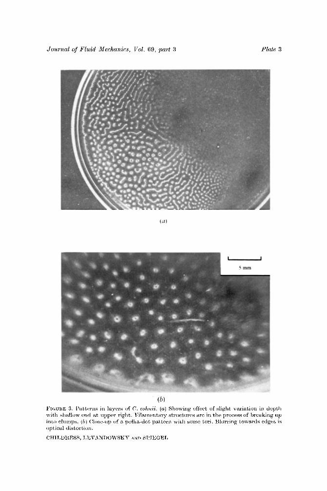
observations of streaming patterns in liquid suspensions of swimming micro- organisms. The phenomenon involves fluid dynamics in that the experiments strongly suggest that the visible patterns of high concentrations of the organisms, as well as the associated motion of the suspending fluid, arise from a process of ‘bioconvection’ (to use the term coined by Platt 1961), wherein natural dissipa- tive losses (presumably due mainly to the viscosity of the fluid) are compensated for by the work done on the fluid by the micro-organisms. Robbins (1952), observing Euglenu graciliis, and Loeffer & Mefferd (1952), observing cultures of the ciliated protozoan Tetrahymena pyriformis, found that patterns formed when the depth of the suspension or the organism number density exceeded critical values.? (Figures 1 and 3 a, plates 1 and 3, show the critical-depth effect.) The type of pattern apparently depends upon the suspension depth and upon the concentration and motility of the organisms. Wille & Ehret (1968), working with

7 The critical values are given as 2 mm and 150 000 organisms/cm3. However, it is not clear whether or not these figures are intended to apply simultaneously at a critical state.

592 S. Childress, M . Leuandowsky and E. A . Spiegel

dense Tetrahymena cultures, observed two distinct steady-state patterns. The polka-dot pattern, in which spherical concentrations of the organism are arranged in a regular array, was formed in relatively shallow cultures (see figures 2 and 3 b, plates 2 and 3). A reticulate pattern emerged in deeper cultures as at the deep end of figure 1. The latter is usually described as consisting of irregular cells (‘regular cell’ being used here to mean a unit repeating periodically along the layer of the suspension), with the organisms swimming predominantly upwards over the interior of the cell, being carried laterally near the top and bottom of the layer, and plummeting downwards in thin vertical columns or sheets which mark the main visible features of the pattern. The concentration within these descending regions can exceed the mean concentration by a factor of 10 or more, and the fluid speed there is typically of the order of lmm/s. This speed appreciably exceeds the mean vertical swimming speed of the organisms (typically 0-5 mm/s in Tetrahymena); thus the organisms in the sheets or columns are swept to the bottom of the layer, eventually to swim again to the top and repeat the process. The pattern formation time is typically 10-30 s, which is also roughly the cycle time of individual organisms within the pattern, and increases as the motility (in the present context, the average swimming speed) of the organisms decreases.

The dynamical explanation of bioconvection that has emerged in recent years (Platt 1961; Winet 1969; Winet & Jahn 1972; Plesset & Winet 1974) lies in the unstable stratification of the organism suspensions. The stratification is caused by the accumulation of organisms near the top of the layer and is a result of the swimming of organisms preferentially in the upward direction. We adopt the biological term and refer to this phenomenon as ‘negative geotaxis’. The occur- rence of negative geotaxis is now well established for Tetrahymena. Since the individual organisms are slightly denser than the ambient fluid, the process can produce an unstable subsurface layer of heavy material.

Plesset & Winet (1974; see also Plesset & Whipple 1974) liken the onset of bioconvection to Rayleigh-Taylor instability. They model the organism-rich sublayer as a layer of dense fluid overlying a less dense, deeper layer of fluid. They study the stability of this system under the influence of viscosity and find that the wavelength of the most rapidly growing mode agrees well with the observed scale of the reticular pattern. This result provides evidence that the onset of bioconvection is indeed due to a density inversion and that growing sedimentation fingers represent the formation of descending columns of organisms.

The model of Plesset & Winet does not directly consider the negative geotaxis of the organisms, nor even their motility, except implicitly as a means by which the unstable equilibrium could be set up. Although it is possible that the negative geotaxib might be inhibited by the formation of the subsurface layer, it is more likely that the mechanism which sets up the layering continues to act as the instability develops and influences the formation of a new stable equilibrium (should any exist), just as temperature differences remain the driving mechanism in nonlinear thermal convection. If the Plesset-Winet model were followed into the nonlinear range, the only possible new equilibrium would be one in which all or a major fraction of the subsurface fluid falls to the bottom, and which has a lighter and therefore stable subsurface layer.

Jourrzul of I''1uiCI MPchanics. Vol. 69, part 3 l'lnte 1

Journal o j Fluid Mechanics, Vol. 69, part 3 Plate 2

BIGURE 2. Pattern formatiori in a 3 inin layer of C. cohnii at a mean coricentration of lo6 organisis/cm3. Tirnea: (a ) 2 s, ( b ) 13 s, (c) 19 s, ( d ) 23 s, (e) 28 s , (f) 32 s , ( 9 ) 36 s , ( h ) 43 s, (i) 2 miri. The siisperision was swirled initially to render it hornogeneoiis arid t lw cxarly patterns are forming during tlie decay of the swirl.

CHlLUHESS, LEVANUOWSKY AND SPlEGEL

Journal of Fluid Mechanics, Vol. 69, part 3 Plate 3

(b) FIGURE 3. Patterns in layers of C. cohwii. (a ) Showing effect of slight \ariation in depth with sliallow v r d at upper right. $“llaincntary structurcs arc in the process of breaking up into clumps. ( b ) (%)sc-iip of a polka-dot piittcrn wit11 sonic t o n . Hliirring towardn ctlges is optical distort i o r i .

CHILDREBS, LEVANDOWSKY AND SPIEGEL

Pattern formation in a suspension of swimming micro-organisms 593

The purpose of the present paper is to develop a simple model for pattern formation by negatively geotactic micro-organisms, based upon the physical picture provided by Winet & Jahn (1972)) but differing from the model of Plesset & Whet in this last respect. A system of equations is proposed in which the layering may be said to be internally generated as an equilibrium solution. Linear and nonlinear stability of this equilibrium solution can then be studied in the usual way. Guided by an analogy with solutes, we replace the discrete organism distribution by a continuous density and incorporate the negative geotaxis as a vertical drift of the organism ‘stuff’ relative to the suspending fluid. We also add an anisotropic diffusion. The motility of the organisms is thus parametrized by a vertical drift U and a diffusivity tensor D, both generally functions of vertical position and the local concentration of the organisms. The production of momentum associated with the locomotion of the organisms is averaged, SO

that the effect of the heavy stuff on the fluid motion is through a negative buoyancy term.

The equilibrium solution in this model describes the vertical stratification induced by the negative geotaxis, and in the present paper we investigate the linear stability of this stratified layer. In 3 2.4 we treat a special case satisfying the atypical condition that the layer depth is small compared with the virtual thickness of the subsurface layer. Some general results concerning the linear stability problem are given in § 3. In 3 4 we treat the case-where the layer depth greatly exceeds the sublayer thickness. A singular perturbation analysis allows us to study the transition from an exact mathematical analogy with BBnard convection under the condition of fixed heat flux to a convective instability with growth rates like those calculated by Plesset & Winet (1974), as the ratio of layer to sublayer thickness is increased. For deep layers we also derive an approximate expression in terms of U and D for the horizontal wavenumber for which growth is most rapid. Analytical details which are included here for completeness but which are not essential to the understanding of results are given in appendices. A discussion of the instability in physical terms is given by Levandowsky et al. (1975). Nonlinear aspects of the model and the construction of steady patterns will be taken up in a separate paper.

2. The model 2.1. Formulation

We consider a horizontally infinite, plane layer of homogeneous fluid bounded by the surfaces z = - H , 0 and containing in suspension a large number of impermeable micro-organisms. We denote the density of the fluid by p and the mean density of an organism by po, and we consider the case po > p . If the fractional volume occupied by organisms is c(r, t ) , the suspension has density p0c + (1 - c) p = p( 1 + ac), where a = po/p - 1. For Tetrahymena Winet & Jahn (1972) give a = 0.09 while the values of c in the cultures discussed above are N This means that density fluctuations in the suspension are small and we describe its motion by the Boussinesq equations

p du/dt + V p -pV2u = - gp( 1 + O ~ C ) k, (2.1) v .u = 0, (2.2)

38 F L M 69

594 8. Childress, M . Levandowsky and E . A . Xpiegel

where u is the suspension velocity, p is the pressure, g k is the acceleration due to gravity and where in view of the smallness of c we have taken the viscosity p to be constant.

To describe the evolution of c we write

dcldt + V . J = 0, (2.3)

where J is the flux of organisms through the fluid. We suppose that this flux consists of a part due to random motions, which is describable by diffusion, and a second part due to the negatively geotactic drift of organisms. Thus we write

J = cU(c,z)k-D.Vc,

D = K ~ ( c , x ) ( i . i+ j . j) + K ( c , z ) k. k, (2.4)

where (i, j, k ) are orthogonal unit vectors and U , K 'and K~ are functions to be specified.

The boundary conditions to be adopted will depend upon the nature of the bounding planes. In all cases we require (with u = (u, v, w) and J = (J1, J2, J3) and suppressing all independent variables but z )

w(0) = w( - H ) = 0, J3(0) = J3( - H ) = 0, (2.5a, b )

which state that the vertical fluxes of fluid mass and of organisms vanish a t both boundaries. We shall take the suspension boundary to coincide with the plane even when the boundary is free, and consider the cases ff (both free), fr (top free, lower rigid) and rr (both rigid), with conditions

a2wlaz2 = 0 on a free boundary, ( 2 . 5 ~ )

awl& = 0 on a rigid boundary. (2.5d)

A final special case will be that of an infinitely deep fluid; there we replace the lower conditions by the requirements that u and c vanish as z -+ - 00.

The central hypothesis of the model, that a continuous function c(r , t ) may replace a complex distribution of self-propelled particles, is certainly a crude simplification of the phenomenon. In the densest parts of the pattern we are dealing with interparticle distances of the order of 10-2 to lO-3cm, yet we wish to resolve pattern structure on the scale of the sublayer thickness, which in typical experiments is about I mm. It therefore seems likely that the averaging envisaged here is over only 10-100 organisms, and that the vertical resolution in determining sublayer distributions (see $2.2) will be a fraction of the sublayer thickness. Another difficulty is that the function D(c, z ) is unknown, and for the most part we take D to be constant. There are certainly substantial errors in such a description of the random component of the organisms' motion. Fortu- nately in the linear stability theory (§§3 and 4) we find that certain important results (e.g. pattern size) are insensitive to the sublayer concentration profile; also, it seems likely that simple diffusion gives a reasonably accurate description over the main body of the layer.


2.2. The equilibrium solution and dejinition of dimensionless variables

It is natural to take the basic pattern-free equilibrium to be a solution of (2.1)- (2.5) which is independent of x, y and t and has u = 0. For such a solution (2.1) determines p for given c and (2.3) and (2.4) integrate (with condition (2.5 b ) ) to give

In this paper we shall refer to two special cases:

cU(c, z ) - K(C, z ) dc/dz = 0. (2.6)

(I) U = U,, K = K ~ , K~ = 6 ~ ~ ; U,, K,,, 6 = constants;

K/U not explicitly dependent on z ; K~ arbitrary.

Evidently, case I1 contains case I; we shall frequently specialize to case I for specific computations. In both of these cases we may integrate (2.6) in the form

(11)

- dc, K(z) = equilibrium concentration profile,

which is an implicit definition of K as a function of z . Using the non-negativity of the integrand we may invert to obtain c = K(z) explicitly, where K is monotone increasing. The positive constant K(0) is arbitrary and is equal to the maximum concentration in the sublayer. Another quantity of interest is the mean concentration c , . We define ...

0 cO = K(O), c, = '1 Kdz.

H -TI For example, in case I we have -

K = coexp(UoZ/KO), co = 7 h eA U,H - 1crn). =----- KO

TO illustrate case 11, consider the family of profiles generated by the choice

K/U = zO(k + 1) (c/cO)k, z,, = constant, (2.9)

where k is a positive number. We have

--+1] ) -z,(k+l)/k < 2 6 0,

(2.10)

k z

K(x) = co [ ( k + 1) 20 i 0, z < - xg( k + l) /k, c, = cOzo/H if H > zo(k+ l)/k.

This family includes the exponential profile (2.8) as the limit for small k and a rectangular profile as the limit for large k, and describes tolerably well the observed profiles.

The equilibrium profiles provide convenient length scales for non-dimensionali- zation. Evidently, KIU is a local scale height and its surface value is

h = Ko/Uo, (2.11a)

where K~ and UO are the values of K and U when z = 0 and c = co. An important dimensionless parameter is the ratio of H to h [cf. (2.8)], which we shall denote by

h = H/h. (2.11 b) 38-2

596 8. Childress, M . Levandowsky and E. A . Xpiegel

However, in case 11, where the profile may have a complicated form, it is sometimes useful to define an equivalent sublayer thickness he by

h e = ( C m / C o ) H (he G H ) , (2.12a)

and to define a corresponding ratio

A, = H/he (A , 2 1). (2.12 b )

If the layer is sufficiently deep, so that K vanishes on the lower boundary or is at least very small there, he will be equal to the thickness of a sublayer of constant concentration co having the same total number of organisms per unit horizontal area as the entire layer.

For the illustration (2.9) and (2.10) of case I1 we see that he = zo if

H > x,(k+ l ) /k .

The occasional advantage of (2.12) over (2.11) as a unit of length will be apparent in $4.4. We refer to a layer having small h (equivalently A, close to 1) as shallow, and one for which A, E h

If Uo is taken as a characteristic speed in the problem, a set of dimensionless variables appropriate to the analysis of the stability of the equilibrium K(z) can be obtained by introducing h as the unit of length:

1 as deep.

r* = h-lr, t* = U0h-lt, U* = U ~ l u , p* = ( h ~ U o ) ( p + p g z ) , } (2.13)

C* = CG'C, K* = K/KO, K: = K1/KO, u* = Ug1 u. The scaling of c, which is already dimensionless, is included for convenience.

In the starred variables (2.13) the equations become

v-l du*/dt* + V*p* - V*'U* = - RG*k,

dc* /d t*+V* . [c"U*k-D* .V*~*] = 0

(2.14 a )

(2.14b)

and the flux condition is

c * ~ * - K * a c * / a Z * = o (2" = 0, - A ) . (2.14 c)

Here a = ./KO (2.15)

is a Schmidt number for vertical diffusion and

R = gat, h 3 / v ~ , = gaC, K i / V ut (2.16)

is a parameter which measures the magnitude of the Archimedean force. We shall refer to R as the 'Rayleigh number' although the parameter of the BBnard problem is m o e closely analogous to the parameter A4R [cf. (2.22)]. The experi- mental data discussed in $ 5 suggest that typical values of a exceed 1 and that values of R are usually in the range 1-100.

2.3. Linear equations

We henceforth drop stars whenever the dimensionless variables (2.13) are used. The dynamical stability of the equilibrium will be studied in the usual way by linearizing (2.14) and separating out time and horizontal space variables. We set


c = K(z) + #(x, y, z , t ) , where q5 is a perturbation, and eliminate the horizontal velocit'y components and pressure by applying the curl operator twice to the linearized momentum equation and ta,king the z component of the result. On substituting

we obtain the equations

($, w) = eYtf(x, y) (Wz), W(z) ) , vy = -a%

(?/a) (D2 - a') W - (0'- a')' JV = GRQ, (2.17)

~@++WDK+D~=+CL~K~@ = 0, (2.18) where D = d/dz and

As is shown in appendix A, this last formula can be rewritten as

9 = K(DK) D[@/(DK)]. (2.19)

The flux boundary conditions are

P ( 0 ) = 9=( - A ) = 0. (2.20)

We show in appendix A that for cases I and I1 (see $2.2) y is necessarily real for solutions of (2.17)-(2.20) with conditions from (2.5). The neutral-stability boundary will therefore be given by a function R(h, a) determined by the condition y = 0. The critical values of R and a, denoted by R, and a,, are determined by minjmizing R for fixed h over all branches and all non-negative a.

2.4. The shallow-layer limit

It appears that bioconvection can only occur when asublayer can in some sense be defined, so the limiting case considered in the present subsection is mainly of formal interest. The stability problem obtained for shallow layers may be used to illustrate the nature of the eigenvalue problem and the method of solution. To avoid inessential complications we consider only case I . If we rescale the (now dimensionless) vertical co-ordinate by A, z = xh (which in effect makes H the unit of length), the equation for K becomes

DK = hK, D = a/&, (2.21)

and for small h we have

This switch in length scale from h to H suggests the change of variables

K = 1 +h.Z+O(h').

h'y= 7, h2W= W , ha = ii,

R4 = h4R = g ~ c , , U a H 4 / ~ ~ ~

in which case (2.17) indicates that the parameter

(2.22)

will replace R. If we now combine (2.18) and (2.19) and allow h to approach zero with barred quantities fixed, we obtain the following problem for shallow layers:

(TI..) (DZ- 3) W- (D2- i i 2 ) 2 w = iF'R,(D, (2.23)

pD+V-D'@+iF28@ = 0, (2.24)

D(D = 0, x = - 1,o. (2.25) -

598 8. Childress, M . Levandowsky and E. A . Spiegel

If 6 = 1 equations (2.23)-(2.25) are identical to the linearized stability equations for a Boussinesq fluid a t a Rayleigh number R, and Prandtl number CT, but with the boundary condition (2.25) on the heat flux replacing the conventional condition CD = 0 corresponding to fixed wall temperature. In this analogue - @ replaces the temperature perturbation, K~ the thermal diffusivity, a the coefficient of thermal expansion and co U,/K~ the equilibrium temperature gradient.

Some calculations for this linear BBnard problem were included in a paper by Hurle, Jakeman & Pike (1967; see also Nield 1968), who showed that a treatment similar to the classical one is possible. As R, is increased, the mode which is first unstable is even in X+ 4, and Hurle et al. found that R4, is 120 for case8 and 720 for case rr, and that the critical wavenumber is zero in each case. Using estimates derived from two variational principles (Chandrasekhar 1961; see also $3) we find that case f r is similar, with R4, = 320 and ii, = 0.

The analysis of the onset of instability is t,hus simpler here in cases f r and rr than in the BBnard problem with conventional boundary conditions, since expansions with respect to CC may be used to study the critical point. To see how these expansions proceed, we first note that (2.24) may be integrated, using (2.25), to dbtain 0 so CDdS(7+6Z2)+/ -1 V d Z = 0. (2.26)

Since we are interested in solutions for small 7 and a, (2.26) suggests that both 7 and should be taken to be O(CC2); (2.23) then suggests that R4 is O(1). We

(7, V ) = a2n+yyn, Wn), a) = c a2nan. (2.27)

-1

thus try CO co

n=O n=O

Substitution gives a sequence of equations starting with

and continuing with systems of the form

mD0 = 0 (2.28)

(2.29)

D2Qn+1 = Yn@o+gn(Wn, ..., w,; Qn-l, ... 7@0; Yn-l, .'.,YO), (2.30)

where fo = 0 and go = Wo + 60,. The boundary conditions follow from (2.5) and (2.25).

Because of the linearity and (2.25) we may take Q0 = I and CDn(0) = 0, n = 1,2, ... . The solutions are obtained a t each stage by computing W,, then 7% and finally CDn+l. Since (2.30) with the boundary condition (2.25) is a self- adjoint problem, the solvability condition for (2.30) is

The resulting, expression for yn is identical to that obtained by substituting (2.27) into (2.26). The series formally determines 7 as a function of R, and a. The calculations are simple and we shall note only the expressions for yo and yl:


Case ff fr rr

Rlc 120 320 720 ac 0 0 0 Y1(Rdc) - 0.0301 - 0.0340 - 0.0368

TABLE 1. Critical parameters for the shallow layer, 6 = 1. yo(&) = 0.

The critical Rayleigh number RdC is thus obtained by solving the simple boundary-value problem for Wo, and y1 can be found once 0, has been obtained. The results for 6 = 1 are given in table 1. Since Y ~ ( R , ~ ) is negative, the point ?i = 0 is a relative minimum of the neutral-stability boundary, and when R, exceeds R,, slightly the growth rate has a local maximum a t the positive wavenumber ( - BrolY1P.

3. General results 3.1. Estimates of R(h, a )

It is shown in appendix A that whenever U / K has no z dependence (case 11) the growth rate y in (2.17) and (2.18) is necessarily real. The analogous statement for the shallow layer was proved by Hurle et al. (1967). Since y then vanishes on the neutral curve, variational principles can be used to eskmate R(h, a ) (Chandra- sekhar 1961); it is known from other similar problems that these approximations (which are upper bounds) can be accurate to within a few per cent for the simplest trial functions. We shall use this method to test the hypothesis that ac = 0 for arbitrary h in case I.

The two variational principles can be stat,ed in term; of real functionals I ( @ ) and Q( W ) defined by

Here Q is a dimensionless viscous dissipation per unit horizontal area and the functions r(z) and g(z) are defined in terms of K(z) , K and I C ~ in appendix A. Then R is given by either of

a2R = min(I(CD)/Q(W)), (D2-a2)2W = --a, Wsatisfies ( 2 . 5 c , d ) , (3.3) rg

a2R = min (Q(W)/I(CD)), CD satisfies (2.18)-(2.20); (3.4) W

the minimum being over all functions satisfying the boundary conditions, and the dependent function ( W and CD in (3.3) and (3.4) respectively) being defined for each trial function as indicated.

In table 2 we show results of calculations with constant U , K , 6 = 1 using @ = 4 in (3.3) and W = sin(nz/h) in (3.4) respectively. Both calculations are for free boundaries. In all cases R had its minimum a t a = 0 and for small h the tabulated

600 8. Childress, M . Levandowsky and E . A. Spiegel

(a)

h ... 0.5 1

a= 0 2459 195-9 0.1 2461 196.3 0.2 2465 197.5 0.3 2471 199.4 0.4 2479 202.2 0.5 2491 205.9 1.0 2585 237.1 2.0 2981 385.3

r - A - 7 2

19-55 19-7 20.2 21.0 22.1 23.7 41.6

128.2

( b ) w-7

0.5 1 2

2465 197.0 19.9 2467 197.3 20.1 2470 198.5 20.5 2476 200.5 21.3 2485 203.2 22.4 2496 206.7 23.9 2588 237.4 38.2 2973 380.2 126.0

TABLE 2. Estimates of R for marginal stability in case I, freefree, 6 = 1. (a) (3.3) used with @ = ez. (b) (3.4) used with W = sinlrzfh.

values bear out the very slow increase of R which is predicted by the values of y1 in table 1.

Estimates of R(h, a ) when h is large but hR is of order unity are given in $4. When h = co, i.e. when the layer is semi-infinite, with free or rigid top surface, the eigenvalue problem may be solved exactly by the series method used in 9 3.3 below. The neutral-stability boundary is shown in tabIe 3, along with estimates of R derived from (3.3) with 0 = ez. For each value of a in the table, wavenumbers smaller than a correspond to growing modeswhen R exceeds the tabulated values.

3.2. Approximate expressions for y

The accuracy of (3.3) rests on the fact that the equation for W is solved exactly. A similar approach can be used to compute'y approximately. Given a trial function @we solve [cf. (2.17)]

(D2 - a2) ( 0 2 - a2q2) W = - a2R@, p2 = 1 + y/a2c. (3.5)

As in the shallow-layer analysis an expression relating y to @ and W can be ,

obtainedbyintegrating (2.18)from - A tooandusing (2.20) (seealso 93.3 below):

A simple choice for @ in case I1 is @ = D K (3.7)

since 9 then vanishes identically. In case I (with K~ = 6 and @ = eZ) the computation is straightforward and gives, in the limit h-too, an implicit equation for y :

-6u2 ( A = 00, free surface). (3.8) 1 2+a( l + q ) (1 +q) ( 1 +a)2 ( 1

This equation was solved numerically and y as a function of a always showed a unique maximum ym (at a wavenumber am). In figure 4 we show ym and am as functions of R, v and 6, or more explicitly, y,/c and am are shown as functions


1.0

a m

0

0.5

5

R b

FIGURE 4. The solid curves indicate (a ) the predicted pattern wavenumber a, and ( b ) the maximum growth rate divided by u as functions of RIG, for &/a = 0 and 0.25, h = co. The curves for the profile parameter k [cf. (2.10)] were obtained from (3.8) for k = 0 and from (3.1 1) for k = a. The plotted points are exact values for k = 0 computed as described in 33.3 for the following parameter values: 0, 8/fa = 0, u = 1 ; 0 , &/a = 0, u = 4; m, &/g = 0.25, G = 4.

of Ro and S / g . Note that the estimates in table 3 for the free-surface case can be obtained by setting y = 0 and 6 = 1 in (3.8).

If the horizontal diffusion term in (2.18) is neglected, the approximation (3.5)-(3.7) can be given a simple physical interpretation. In neglecting diffusion we nevertheless retain the sublayer thickness h as a parameter and regard K as an arbitrary prescribed concentration profile. Then CD as defined by (3.7) determines an infinitesimal vertical shift of K(z) as the inktability develops,? and (3.6)

(3.9)

Viewed in this way y is the growth rate for a prescribed concentration profile, the process by which the stratification was established having disappeared from the problem. This provides a way of looking at the model studied by Plesset & Winet

is replaced by 0 1 ( y+ W ) D K d z = 0. - A

(3.10)

With (3.10) substituked in (3.9), y = - W(1) and (3.5) can be solved to obtain the following equation for infinite depth:

y 2 + a 2 a y ( l + q ) = Rag/(l+cotha) ( A = 8, free surface). (3.11)

This expression agrees with that given by Plesset & Winet if the q appearing on the left is replaced by 1. Curves based on (3.11) are shown in figure 4. Note that (3.11) is in fact an exact result when all diffusion and the negative geotaxis are neglected. This is because (3.9) with (3.10) is then equivalent to (y + W ) DK = 0.

t Physically, 0 = DK corresponds to a modulated vertical shift of the equilibrium concentration, and can be generated by K ( z + f e Y t ) for smallf(z, y).

602 S. Childress, M . Levandowsky and E . A . Spiegel

Rigid

a Computed 2( 1 +a)*

0 2.00 2.00 0.05 2.41 2.43 0.10 2.83 2.93 0-15 3.29 3.50 0.20 3.80 4.15 0.40 6.53 7.68 0.60 10.83 13.11 0.80 17.23 21.00 1.00 26.26 32.00

Free - Computed 2 4 1 + a)3

0.00 0.00 0.12 0.12 0.26 0.27 0.45 0.46 0.67 0.69 2.07 2.20 4.60 4.92 8.69 9.33

14.85 16.00

TABLE 3. Computed and estimated values of R for a fluid of infinite depth, case I, 8 = 1, for the upper surface rigid and free. The formulae follow from (3.3) with CD = ez.

3.3. Solution for inJinite depth, case I To solve the eigenvalue problem exactly for h = co, we write

w = A1 W1-k A2 j< + A3 1r39

where the are solutions of

(y + 6a2 + D - D2) (D2 - a2 ) ( 0 2 - a2q2) W = a2Re2: W

We take rn

n=O

p l = a, p 2 = aq, p 3 = +{I + [i + 4(Sa2 + y ) ] i ) .

The boundary conditions are

W = D 2 W = ( D - 1 ) ( D 2 - a ~ ) ( D 2 - a 2 q 2 ) W = 0 , z = O .

Thus y can be found by applying Newton’s method to a 3 x 3 determinant. Numerical results show the expected dependence on (T when a, and ym/g are expressed as functions of R/(T and S/g. The exact values of a, and y,/v agree reasonably we11 with the approximate values calculated as in $3.2, the largest discrepancy in a, occurring for 6 = 0, where the error is 7 % for (T = 4. Errors in y,/a are less than 3 % for (T = 0, but for 81.- = 0.25 the exact value is larger than the approximate one by 15% a t R = 8, (T = 2 (see figure 4). We recall that exponential and square profiles are two extreme cases within the family (2.10) of concentration profiles which might be considered representative in this problem.

3.4. Computation of R,(h)

We turn now to the h dependence of the critical Rayleigh number. In view of the estimates in $3.1 the conjecture a, = 0 appears to be reasonable in case I. We have not been able to show that this is true generally, but we shall show here that quite generally R(h, 0) is finite and positive. Assuming that the conjecture holds and R,(h) = R(h,O), our sufficient condition for instability gives the critical Rayleigh number.


h 0.5 1.0 1.5 2.0 2.5 3.0 4.0 5.0 7.0

10.0 00

ff 2 459.0

195.9 49.04 19.55 10.03 6.017 2.883 1-734 0.892 0.492 0.000

f r 6213.0

470.2 122.2 42.82 21.09 12.19 5.481 3.132 1.494 0.771 0.000

r r

14 790.0 1185.0

300.0 121.3 63.37 38-82 19.54 12.44 7.244 4.808 2.000

TABLE 4. R,(h)/c? for case I, with two free surfaces, one rigid and one free or both rigid.

The analysis follows the scheme outlined in $2.4. Expansions of the form

a3 a3

(7) W ) = a2n+2(yn, K), 0 = 2: a2Qn n=O n=O

are substituted into (2.17)-(2.20)) and R(h, 0) is obtained by setting yo = 0. One analytical point requiring comment concerns the form of the solvability condition. The problem for 0% is now

D.Fm = - ~ ~ @ ~ + g ~ , gn = -K(DK)D(@/DK), (3.12a)b)

Sn = 0) 2 = --h)O) ( 3 . 1 2 ~ )

QO(O) = 1) CD,(O) = 0, n 3 1. (3.13)

The boundary-value problem which is adjoint to tbe homogeneous version of

D[K(DK)DY] = 0) (3.14 a ) (3.12) is

D Y = 0, z = -h,O. (3.14b)

The solution for this problem is Y = constant. The solvability condition is therefore again obtained a t each stage simply by integrating the equation for Qn [cf. (2.26) and (3.6)].

The remainder of the calculation is straightforward and there results

y , , [ l -X( -h)] -R/o - A (DzTl(,)zdz+/o - A K ~ D K ~ z = 0, ( 3 . 1 5 ~ )

where D4WO = DK with Wo = 0, OWo or DzWo = 0 for z = -h,O. (3.15b)

For case I the values for &(A) are given in table 4. We find

3, q 4 p 4 ) A + 0,

where Dl = (120, 320, 720) in cases (#)ff,r) rr) in agreement with the shallow-layer theory. We also note that for a free upper surface

R, WZlh, + a, (3.16)

where pz = (3 ,4) for a (free, rigid) lower boundary. Thus a free sublayer on a sufficiently deep layer is always unstable. If R is fixed and the upper surface is

604 S. Childress, 1M. Levandowsky and E . A . Spiegel

free, there is, moreover, a value of h (and hence a value of H ) below which the layer is stable. For fixed A, there is correspondingly a value of R (hence eo) below which the layer is stable. The last statement remains true if the reference concentration in (2.14) is taken to be the mean concentration e, rather than co; this change in effect multiplies the tabulated values of R, by (1 - e-h)/h.

4. Singular perturbation for deep layers 4.1. Remarks

The calculations given in ss3.2 and 3.3 describe the nature of the linear stability in deep layers when R is O( 1) (that is, when R is significantly greater than R,); there the maximum growth rate presumably gives an indication of pattern size. At the critical boundary, on the other hand, the onset of instability resembles a typical convective instability but with the unusual property that a, = 0. Our aim in the present section is to study the transition between these two distinct regimes in a parameter range for which a perturbation analysis is feasible.

Such an analysis is motivated by observations of pattern formation in slightly tilted containers (see figure 1). Since the layer depth then varies linearly and rather slowly, one would expect to see rather large-scale structures near the critical depth (where a, is very small), followed by a gradual reduction of pattern size until the value appropriate to infinite depth-is reached. What is in fact observed is an abrupt appearance of a well-defined horizontal scale (determined by the spacing of polka dots or columns) with no noticeable transition through small wavenumbers.

The key to a study of the transition region in deep layers is the introduction of the limit process

h-tm with B = h R , & = h a , $7=h2yfixed (4.1)

in place of the expansion for small a. In particular the horizontal wavelength will be of the order of the layer depth in the transition region. The justification for the choice (4.1) is the following: for h >> 1 the behaviour of R, is given by (3.16), suggesting that 8 is the proper O(1) Rayleigh number in the transition region. Moreover, near a = 0 on the neutral-stability boundary we expect to have R - R, = O(a), and in order to be able to resolve the transition we shall therefore want a - A-l. Finally, the definition of p is suggested by (3.6) when tilde variables are substituted. (Physically we expect the maximum growth rate to be established by the effect of horizontal diffusion, which is O(a2) in (3.6).) If the quantities (4.1) are introduced into (3.8) we obtain in the limit (v is fixed and O(1))

p = d R / ( 1 + q ) - 6E2, q 2 = 1 + y/&. ( 4 4

We shall show that (4.2) is an asymptotic result provided that 8 and 6 are numerically large, with B/& = O(1). Thus in a sense (4.2) is the asymptotic (for large 8) form of a certain equation we wish to determine, the latter equation providing the dependence of $7, upon a right up to the critical value A, (note that B, = 4 for case fr).


4.2. Construction of matched expansions

The analysis is facilitated by the use of matched asymptotic expansions, since the sublayer (or inner) region requires special attention, while the flow in the main body of the layer (the outer region) has an especially simple structure. The correct choice of outer variable is suggested by the momentum equation (2.17) written in the variables (4 . I) :

0 4 W = A-2a"2( 1 + q2) 0 2 W - A-3G2BO - h-4cX4q2W. ( 4 . 3 ~ )

The corresponding equation obtained from (2 .18) is, in case I,

D 2 0 - DO = ez W + h-2(j7 + &cX2) O. (4 .3 b )

For (4 .3 a ) there is a simple limit as h-tco, namely

D4W = 0.

However, it is clear that this limit is not valid uniformly over the layer and we introduce an outer variable which makes D2 formally of order

z" = x/h = O(1) (outer region). (4 .4)

The fact that limits with z" fixed are clearly non-trivial provides additional evidence that d is the correct O( 1 ) wavenumber in the transition region.

If (4 .3a ) is written in terms of the outer variable we have

( D - 5 2 ) ( D 2 - 6 2 q 2 ) w = -hd2R07 D = d/dz". (4.5)

In view of (4 .3 b ) it is reasonable to expect that, in case I, O is exponentially small in the outer region (a fact already suggested by the expansions in a), so that (4 .5 ) reduces to

We shall apply a particular ordering of W and O formally and show that the required matching can be carried out using standard methods (Cole 1968, chap. 1). We consider case I first.

( D ' 2 4 2 ) (D2-62q2) w = 0. (4 .6)

Inner expansions having the forms

W = h-2Wo + k3W, + h-4W2 + . . . , O = @,+h-1O1+h-2O2+...

(4.7 a ) (4.7 b )

are introduced, and we consider an outer solution of (4 .6):

@ = h-l[A(h)sinhbz"+B(h) coshBx"+C(h)sinhdqz"

+ D(h) C O S ~ a"@] - + + . . . . (4 .8 )

The boundary conditions on the lower wall require

r n ( - 1 ) = o , BVn(-l) or D2Rn(-1)=o. (4 .9 )

Substitution of (4 .7 ) into (4 .3 a, b ) with the help of the conditions on z = 0 gives a series of easily solvable problems and we have for the first two terms

W, = ~ r , z + , 8 ~ 2 ~ ,

1~ = d 2 W ( i + ~ 2 2 - e z ) + ~ r ~ 2 + , 8 ~ 2 3 . (4.10) I Oo = eB,

O~ = 0,

606 X. Childress, M . Levandowsky and E. A . Xpiegel

Here a, and P, are arbitrary constants. To indicate how these constants are determined by matching, we consider the outer expansion of the inner partial sum of W up to terms of order h-3, obtained simply by discarding exponentially small terms:

h-Z%+h-3K = h ~ , X ” 3 + ~ 1 & 3 + h - ~ ( a 0 & + g d ~ ~ & 2 ) +O(h-2). (4.11)

The addition of the term h-4W2 to the left side would add a polynomial to the right side, but it is apparent that only multiples of Z5, E4 and Z3 respectively could thereby be introduced into terms of order A , I and h-l, with even higher powers coming from subsequent terms. Thus the terms on the right side of (4.11) must coincide with terms of these orders in the power series for m. Now since (4.9) must be satisfied, the term of leading order in (4.11) cannot be a multiple of Z3. Hence Po = PI = 0. The last term on the right side of (3.11) gives the three conditions (withA = A,+h-lA,+..., etc.)

B,+D, = 0, Bo+q2D, = R, (4.12 a)

A, + qc, = a&. (4.126)

The first two of these, along with two Conditions from (4.9), determine mo uniquely, while the last determines the remaining constant a,. To complete the calculation, the equation for 9, valid to order 1, folIows from integration of ( 4 . 3 ~ ) with H i = a,z:

7 = a, - 662.

Solving for A,, ..., Do using (4.6) and ( 4 . 1 2 ~ ) ) and evaluating a, from (4.12b) we obtain

7 = dRQ(d , q) - 662, (4.13) where, for case f r ,

1. (4.14) sinh d sinh dq - 2q cosh d cosh dq + 29

q sinh a” Gosh d q - cosh d sinh dq G(d ,q ) = -

This is the desired equation for the growth rate, valid through the transition region as discussed in 5 4.1.

Before considering (4.13) in detail we indicate how the higher-order terms can be found. In order to determine the equation for 7 to terms of order h-n inclusive, inner terms up to W,,, must be obtained. (Actually for the last term only D2W,+, need be known.) Each of these can be written as a finite sum of the form po(z) + ezpl(z) + . . . + emap,(z), where the pi are polynomials. Only p, enters the matching: If we now suppose that a,, ..., a,-,, Po, ..., P, are known, then the coefficients of zo and z2 in the outer expansion of ... +h-(n+3)Wn+, are known up to terms of order h-Cn+l). The corresponding matching conditions, along with the two conditions (4.9) on the lower wall, are then sufficient to determine m,, and czn can be found by matching the term in 2. Finally P,,, is obtained by matching with the Z3 term in Fn-,. We have carried out these calculations for n = 2 and record the results in appendix B.


0 4 A

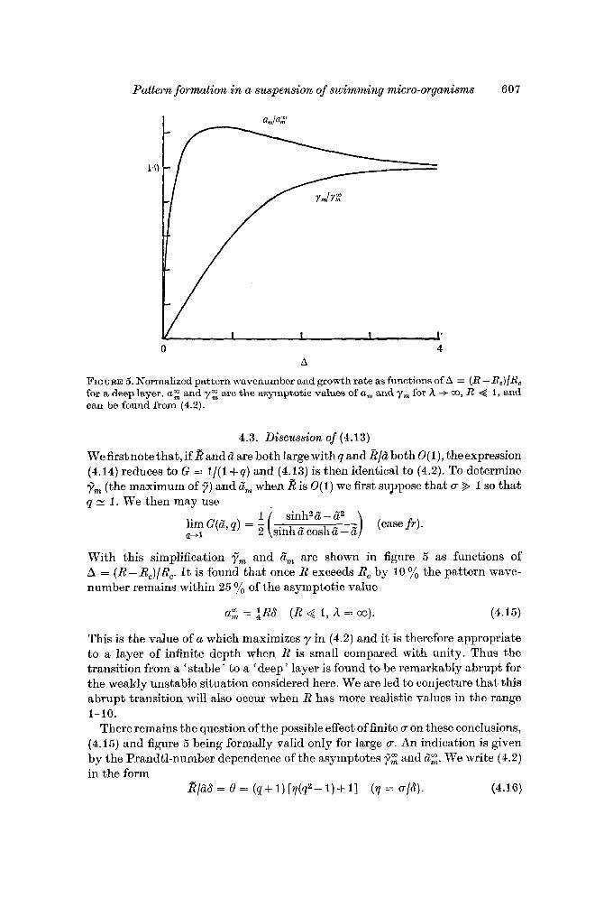
FIGURE 5. Normalized pattern wavenumber and growth rate as functions of A = (R - R,)/R, for a deep layer. a: and y: are the asymptotic values of a, and ym for h -+ m, R < 1, and can be found from (4.2).

4.3. Discussion of (4.13)

Wefirstnotethat,ifBandiiare bothlargewithqandBl6 bothO(l), theexpression (4.14) reduces to G = 1/(1 +q) and (4.13) is then identical to (4.2). To determine yrn (the maximum of j7) and Zm when 2 is O(1) we first suppose that cr >> I so that q -N 1. We then may use

(case f r ) . sinh2 6 - 1.2

limG(6,q) = - q-1

With this simplification f r n and a“, are shown in figure 5 as functions of A = (R - Rc)/Rc. It is found that once R exceeds Re by 10 yo the pattern wavenumber remains within 25 yo of the asymptotic value

a: = $RS (R < I , h = CO). (4.15)

This is the value of a which maximizes y in (4.2) and it is therefore appropriate to a layer of infinite depth when R is small compared with unity. Thus the transition from a ‘stable’ to a ‘deep’ layer is found to be remarkably abrupt for the weakly unstable situation considered here. We are led to conjecture that this abrupt transition will also occur when R has more realistic values in the range 1-10.

There remains the question of the possible effect of finite cr on these conclusions, (4.15) and figure 5 being formally valid only for large cr. An indication is given by the Prandtl-number dependence of the asymptotes 7% and 6:. We write (4.2) in the form

(4.16) B/GS = 0 = ( q + 1) [y(q2- 1) + 11 (y = +).

608 S. Childress, M . Levundowsky and E. A . Spiegel

Differentiating (4.16) with respect to B and setting dyldG = 0 we obtain a second equation in q and 8:

Eliminating q from the last two equations produces a quadratic equation for ~ ( 0 ) :

g ( e - p ) 7 2 + ( - 2e3+ 1002- ioe- i )r + 1 = 0. (4.17)

Examination of the real roots of (4.17) shows that when 7 > 3j (on the basis of estimates given in $5, 8 is a satisfactory lower bound) the parameter 8 varies between 2 + 4 3 and 4, the latter corresponding to cr = co [cf. (4.15)]. Thus a; is within 8 % of the value at CT = co when cr exceeds $8. The quantity yz21R2 varies from 0-041 to 0.0625 as crlS increases from $ to a. Consequently, in the limit considered here the effect of (r on the development of the instability is not very significant.

42+( i -o )q++e = 0.

4.4. Case I1

We now consider the effect of the choice of U and D upon the first-order expression (4.13) for the growth rate. We shall show that, if we define (still in the dimension-

8 = 1 K 1 ( K , z ) DKdz

and use the equivalent sublayer thickness defined by (2.12a) in place of h in the definition (2.13) of the starred variables, then (4.13) holds also in case 11.

The proof hinges on the fact that the exact form of K(z) enters into the computation of a0 only through the term z2 in the outer expansion of the inner W,; this term contributes the only inhomogeneous matching condition at that order. Now in case I1 we have @, = DK and therefore

less variables (2.13)) 0

--A*

D2JK = - d z 2 I z K ( z ) d z + d 2 R I 0 - -A# K(i )dz ,

which immediately gives the coeEcient of 3 in the outer expansion of W,. If (4.13) is to be unchanged we must have

--A,

0 K(2)d.z = 1. (4.18)

But (4.18) follows from the choice of he as the unit of length, since (4.18) and ( 2 . 1 2 ~ ) are then equivalent. The above definition of 8 follows easily from the integral of (2.18) with W = W, and @ = Do = DK, with @,(O) taken as unity.

S- -Ae

5. Discussion The measurements of Winet & Jahn (1972) and the data reported by Plesset

& Winet (1974) (see table 5 below), both for Tetruhymenu pyriformis, provide estimates of the values of the dimensionless parameters in typical Tetruhymena cultures. The variable c should be regarded as the volume density of only those organisms which actively participate in the pattern (here, the negatively geotactic organisms). A proper determination of c, U , K and K~ would presumably


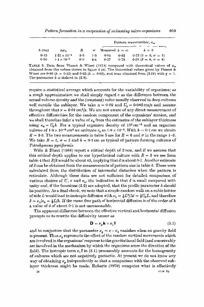
Pattern wavenumber, a, r

0.15 1.21 x 5.9 1.5 0.94 0.92 0.73 (8 = 0, U = 1) 0.05 1.1 x 6.0 4.4 0.57 0.70 0.69 (8 = 0, = 4)

TABLE 5. Data from Plesset & Winet (1974) compared with theoretical values of a, obtained from the values shown in figure 4 (a). The theoretical values given by Plesset & Winet are 0.86 (h = 0.15) and 0.65 (h = 0.05), and were obtained from (3.11) with q = 1. The parameter k is defined in (2.9).

h > h (-1 agco R u Measured k = co k = O

require a statistical average which accounts for the variability of organisms; as a rough approximation we shall simply regard c as the difference between the actual volume density and the (constant) value usually observed in deep cultures well outside the sublayer. We take a = 0.09 and U, = 0-045cm/s and assume throughout that v = 0.01 cm2/s. We are not aware of any direct measurement of effective diffusivities for the random component of the organisms’ motion, and we shall therefore infer a value of K, from the estimates of the sublayer thickness using K, = U,h. For a typical organism density of 105cm-3 and an organism volume of 1-8 x 10-Scm3 we estimate co as 1.8 x With h = 0.1 cm we obtain R = 3.5. The two measurements in table 5 are for R = 6 and CT in the range 1-5. We take R = 5, CT = 2 and h = 0.1 cm as typical of pattern-forming cultures of Tetrahymena pyriformis.

Wille & Ehret (1968) report a critical depth of 2 mm, and if we assume that this critical depth applies to our hypothetical culture with R = 5 we see from table 4 that R/S would be about 45, implying that Sis about 0.1. Another estimate of 6 can be obtained from the measurements of pattern size in table 5 . These were calculated from the distribution of internodal distadces when the pattern is reticulate. Although these data are not sufficient for detailed comparison of various choices of U , K and K ~ , the indication is that 6 is small compared with unity and, if the functions (2.9) are adopted, that the profile parameter k should be positive. As a final check, we note that a simple random walk on a cubic lattice of side L would lead to isotropic diffusion with K~ = QL2/At = QUO L, and therefore 6 = K , / K ~ = QL/h. If the mean free path of horizontal diffusion is of the order of h a value of S of about 0.1 is not unreasonable.

The apparent difference between the effective vertical and horizontal diffusion prompts us to rewrite the diffusivity tensor as

D = Kuk+K1l (5.1)

and to conjecture that the parameter K~ = K - K~ vanishes when no gravity field is present. Thus K~ represents the effect of the random vertical movements which are involved in the organisms’ response to the gravitational field (and conceivably are involved in the mechanism by which the organisms sense the direction of the field). The isotropic term K~ I in (5.1) presumably accounts for the homogeneity of cultures which are not negatively geotactic. At present we do not know any way of obtaining K~ independently so that a comparison with the observed sublayer thickness might be made. Roberts (1970) computes what is effectively

39 F L M 69

610 S. Childress, M . Levandowsky and E. A . Spiegel

a sublayer thickness for negative geotaxis of Paramecium, basing his calculation on the idea that the preferred orientation of the body is induced by its shape and density distribution. This is a restrictive assumption but Roberts’ result is com- patible with (5.1), in the sense that it shows one way of relating vertical diffusion directly to the response of the organism to the gravitational field. In any case, even for non-identical organisms, dispersion in the motility can be modelled in terms of these diffusion constants.

A related example of the combined effect of random and directed motion of organisms, leading to the formation of macroscopic structures, was studied in a continuum model by Keller & Segel (1970). In their work an equation similar to (2.4), involving a chemotactically induced flux of organisms, was coupled with diffusion-reaction equations. Their chemotactic flux, proportional to the gradient of concentration of a chemical, corresponds to our geotactic flux kcU. The analogy suggests that the latter term may also be best regarded as proportional to a gradient, in particular to the pressure gradient. In the dilute limit c < 1 this altered form would be equivalent to (2.4), but in general there would arise new physical effects, such as horizontally directed ‘ barotactic swimming ’. Advan- tages of using the pressure-gradient form may appear, even in the dilute case, if centrifugal acceleration is important. (Some very preliminary observations of pattern formation on a rotating turntable indicate that patterns may be modified by rotation.) In addition, it is not impossible that actual chemotaxis is sometimes involved in pattern formation by swimming micro-organisms (Brinkman 1968).

Returning to the present results, we see on comparing table 4 and figure 5 that we can estimate the width of the transition from a marginally stable to a ‘deep’ culture as H changes slowly with x. We assume that R is constant and that the small R theory can be applied to the transition even though R, is not small. For the culture with R = 5, a critical depth of 2h and 6 = O-l:we see that once the depth has increased to 3h the value of R, has dropped to about 1.2, making A in figure 4 about 1. This suggests that the critical depth is marked by a transition region in which the depth changes by no more than 0.5 mm. In some of our typical experiments with Tetrahymena we observed critical depths of about 4.5 mm, which, if S is again assumed to be 0.1, would indicate an R of only about 0.4, but nevertheless a value A = 0.25 was reached a t a depth of 5mm.

The linear stability problem considered in this paper is an idealization which cannot be completely realized in experiments, whether in tilted layers or in initially stirred, deep cultures. The sublayer forms in a time of the order of HIU, - 30 s, and if R is between 1 and 5 the equilibrium envisaged here presumably never has a chance to form completely. The transient nature of the convective instability is emphasized by the description of column formation given by Winet & Jshn (1972).

A related thermal instability has been analysed and observed by Foster (1965, 1969). He considered BBnard convection in a layer cooled from its top boundary. The formation of a cool zone at the top is clearly analogous to sublayer formation, and the onset of what Poster called “manifest convection”, involving the abrupt falling away of thin sheets of cool fluid from the top layer, is similar to the rapid transition in a tilted layer envisaged in 54.3, the horizontal co-ordinate there

Pattern formation in a suspension of swimming micro-organisms 61 1

taking the place of the time variable in the thermal instability. In detail the two problems are different, but in a broad sense the physical description of the instability is the 5ame.t Other dynamical analogies are suggested by observations of sedimentation of swarms of inert particles in a viscous fluid and by the behaviour of fluidized beds operating a t small particle Reynolds number, but owing to differences in the boundary conditions neither of these analogies is exact.

The structure of bioconvection patterns following the initial instability considered above is likely to be a complex and nonlinear process since the Reynolds number based on U, and H is typically in the range 1-5 and any new steady equilibria are quite different from a simple vertically stratified layer. The application of the present model to this problem, and to the construction of steady solutions similar to the polka-dot patterns discussed in $ 1 , will be taken up in a separate paper.

The authors wish to thank S.H.Hutner and colleagues at the Haskins Laboratories a t Pace University for their enthusiasm and assistance. They are indebted also to J. B. Keller, P. H. Roberts, Melvin Stern and Howard Winet for helpful conversations and to L. Baker, G. Baran, E. Graham and Rory Thomson for assistance with numerical work. This work was supported by NSF grants GP-32996x a t New York University and GP 32336x at Columbia University, and NIH grant GRS FR-35596 a t Haskins Laboratories.

Appendix A. Integral identities of linear theory

and integrate with respect to z from - h to 0 to obtain Multiply (2.17) by W* (where * means 'complex conjugate' in this appendix)

Now differentiate condition (2.6) and evaluate the result for c = K(z):

] D K - K ( K , z ) D ~ K = 0. (A 2) au a K au a K D K

Note that the first bracketed term in (A 2) vanishes for both case I and case I1 since

With the help of (A 2) and (A 3), note that (2.19) can be rewritten as

Using this expression and (2.20), we multiply @/DK by the complex conjugate of (2.18) and integrate to obtain

%= -K(DK) D(@/DK).

t (Note added in proof.) Other methods of generating a relatively heavy sublayer as a model for the initial bioconvective instability were considered by H. Wager (191 1).

39-2

612

If we subtract a2R times (A 4) from (A 1) and take the imaginary part we find

8. Childress, M . Levandowsky and E. A . Spiegel

Im(y) [u2R/' - A (DK) -1 (@12dz+n-1 /o - A ( ~ D W [ 2 + u 2 1 W ~ z ) d z ] = 0, (A 5)

which establishes that y is real. A partial integration of (A 4) yields

where I(@) is given by (3.2) with

The variational principles (3.3) and (3.4) follow from (A 1) and (A6) with y = 0 by computing the first variation and essentially reversing the steps in the above derivation.

Appendix B. Matched asymptotic expansions for a deep layer, case I, ,ff',,fr;a = Xa,B = AR,? = A2y, A-+m

Inner expansions

42 = i + y / i ~ g , = @, + A-w, + o(A-~) , w = A-2( w, + A-lW, + A-ZW, + A-3W3) + O(A--6),

W, = a,z, W, = a2Bp + $ z 2 - e ~ ] , W, aZz+pzz3,

(Do = ez, QZ = &zoz2ez,

W3 = G4R( 1 + q2) (32' +&z4 - ez) - a,62~ez(&2 - 42 + 10)

+ 1 O a , 6 ~ B + $ i ~ ~ a 0 z ~ + c g z .

Outer expansions

r, = A , sinh dz" + B, cosh 62 + C, sinh Cqx" + 0, Gosh dqz".

x" = Z/A, w = h-l[Vo + A-~TTQ + o(A-~) ,

The constants in the above are given by the following expressions:

a0 = dRG(d,q) , a2 = d(Az+pCz) , p2 = $d2(Ao+~3CO).

a3 is determined by matching at the next stage. In the expression for a, the function B is given by (4.14) for casefr and by

1 q sinh d cosh dq - cosh a" sinh dq sinh 6 sinh dq

G(d,q) = - 92- l [ 1

for case 8. We give the coefficients in the outer expansion for case f r onIy:

A , = [I'B/(qz- I)] [qcoshdcoshdq-sinhdsinhdq-q],

I' = [cosh d sinh dq - q sinh d cosh dq]--l,

Pattern formation in a suspension of swimining micro-organisms

C, = [I'B/(q2 - I)] [cosh a" cosh a"q - q sinh a" sinh n"q - 11,

A , = (3a, + d2q2) A , + d21'R[sinh a" sinh 6q - q cosh a" cosh Bq],

61 3

D, = -B, = B/(q2- I),

c, = (301, + ~ 2 ) c, + 6r8, D, = (3a, + ~ 2 ) D,, B, = 622 - D,.

The equation for 7 up to terms of order h-, is found to be

7 = iiRG(6, q) - 662 - h-I(ga"2B)

+ P [ ( q 2 - 6)63fiG(a", q) + 3a"2w2G2(a", q) + ii3RG1(a", q)] + O(h-3),

coth(d), case f f7

-I'(q2- I)sinha"sinh6:q+G(a",q), casefr. where

R E F E R E N C E S

BRINKMAN, K. 1968 Keine Geotaxis bei Euglena. 2. Pjlanzen Physiol. 59, 12-16. CHANDRASEKHAR, S. 1961 Hydrodynamic and Hydromagnetic Stability, chap. 2. Oxford

COLE, J. D. 1968 Perturbation Methods i.n Applied Mathematics. Blaisdell. FOSTER, T. D. 1965 Onset of convection in a layer of fluid cooled from above. Phys.

Fluids, 8, 1770-1774. FOSTER, T. D. 1969 Onset of manifest convection in a layer of fluid with time-dependent

surface temperature. Phys. Fluids, 12, 2482-2487. HURLE, D. T. G., JAKEMAN, E. & PIKE, E. R. 1967 On the solution of the BBnard

problem with boundaries of finite conductivity. Proc. Roy. SOC. A 296, 469-475. KELLER, E. F. & SEGEL, L. A. 1970 Initiation of slime-mold aggregation viewed as an

instability. J . Theor. Biol. 26, 399-415. LEVANDOWSKY, M., CHILDRESS, S., SPIEGEL, E. A. & HUTNER, S. H. 1975 A mathematical

model for pattern formation by swimming microorganisms. J . Protozool. 22, 296-306. LOEFFER, J. B. & MEFFERD, R. B. 1952 Concerning pattern formation by free-swimming

microorganisms. Am. Naturalist, 86, 325-329. NIELD, D. A. 1968 The RayleighJeffreys problem with boundary slab of finite con-

ductivity. J . Fluid Mech. 32, 393-398. PLATT, J. R. 1961 'Bioconvection patterns' in cultures of free-dwimming microorganisms.

Science, 133, 1766-1767. PLESSET, M. S. & WHIPPLE, C. G. 1974 Viscous effects in Rayleigh-Taylor instability.

PLESSET, M. S. & WINET, H. 1974 Bioconvection patterns in swimming microorganism cultures as an example of Rayleigh-Taylor instability. Nature, 248, 441-443.

ROBBINS, W. J. 1952 Patterns formed by motile Euglena gracilis var. bacillaris. Bull. Torrey Bot. Club, 79, 107-109.

ROBERTS, A. M. 1970 Geotaxis in motile microorganisms. J . E x p . Biol. 53, 687-699. WAGER, H. 1911 On the effect of gravity upon the movements and aggregation of

Euglena viridis, Ehrb. and other micro-organisms. Phil. Trans. B 201, 333-390. WILLE, J. J. & EHRET, C. F. 1968 Circulation rhythm of pattern formation in populations

of a free-swimming organism, Tetrahyrnena. J . Protozool. 15, 789-792. WINET, H. 1969 The influence of gravity and origin of bioconvection in Tetrahyrnena

pyriformis cultures. Ph.D. thesis, University of California, Los Angeles. WINET, H. & JAHN, T. L. 1972 On the origin of bioconvective fluid instabilities in Tetra-

hynaencc culture systems. Biorheol. 9, 87-94.

University Press.

Phys. Fluids, 17, 1-7.

Journal of Fluid Mechanics - University of · PDF fileJournal of Fluid Mechanics ... The...

Documents

Transcript of Journal of Fluid Mechanics - University of · PDF fileJournal of Fluid Mechanics ... The...