Journal of Financial Economics - Duke...

Contents lists available at ScienceDirect

Journal of Financial Economics

Journal of Financial Economics 118 (2015) 113–134

http://d0304-40

☆ ThegratefulseminarSCOR/IDChicago

n CorrE-m1 Te2 Te3 Te

journal homepage: www.elsevier.com/locate/jfec

Tail risk premia and return predictability$

Tim Bollerslev a,b,c,n,1, Viktor Todorov d,2, Lai Xu e,3

a Department of Economics, Duke University, Durham, NC 27708, United Statesb NBER, United Statesc CREATES, Denmarkd Department of Finance, Kellogg School of Management, Northwestern University, Evanston, IL 60208, United Statese Department of Finance, Whitman School of Management, Syracuse University, Syracuse, NY 13244-2450, United States

a r t i c l e i n f o

Article history:Received 9 May 2014Received in revised form29 September 2014Accepted 18 February 2015Available online 26 July 2015

JEL classification:C13C14G10G12

Keywords:Variance risk premiumTime-varying jump tailsMarket sentiment and fearsReturn predictability

x.doi.org/10.1016/j.jfineco.2015.02.0105X/& 2015 Elsevier B.V. All rights reserved.

research was supported by a grant from the Nto an anonymous referee for her/his veryparticipants at NYU Stern, the 2013 SETA MEI conference on Extreme Events and Unceand University of California Berkeley for thesponding author at: Department of Economail addresses: [email protected] (T. Bollerslevl.: þ1 919 660 1846.l.: þ1 847 467 0694.l.: þ1 315 443 3602.

a b s t r a c t

The variance risk premium, defined as the difference between the actual and risk-neutralexpectations of the forward aggregate market variation, helps predict future marketreturns. Relying on a new essentially model-free estimation procedure, we show thatmuch of this predictability may be attributed to time variation in the part of the variancerisk premium associated with the special compensation demanded by investors forbearing jump tail risk, consistent with the idea that market fears play an important rolein understanding the return predictability.

& 2015 Elsevier B.V. All rights reserved.

When the VIX is high, it's time to buy, when the VIX is low,it's time to go.

Wall Street adage

SF to the NBER, and CREATEuseful comments. We wouldeetings in Seoul, South Korertainty in Insurance and Fieir helpful comments and suics, Duke University, Durha

), [email protected]

1. Introduction

The VIX is popularly referred to by market participantsas the “investor fear gauge.” Yet, on average, only a smallfraction of the VIX is arguably attributable to market fears.

S funded by the Danish National Research Foundation (Bollerslev). We arealso like to thank Caio Almeida, Reinhard Ellwanger, Asaf Manela and

a, the 2013 Workshop on Financial Econometrics in Natal, Brazil, the 2014nance in Paris, France, the 2015 Midwest Finance Association meetings,ggestions.m, NC 27708, USA.du (V. Todorov), [email protected] (L. Xu).

www.sciencedirect.com/science/journal/0304405X

www.elsevier.com/locate/jfec

http://dx.doi.org/10.1016/j.jfineco.2015.02.010



http://crossmark.crossref.org/dialog/?doi=10.1016/j.jfineco.2015.02.010&domain=pdf



mailto:[email protected]




T. Bollerslev et al. / Journal of Financial Economics 118 (2015) 113–134114

We show that rather than simply buying (selling) whenthe VIX is high (low), the genuine fear component of theindex provides a much better guide for making “good”investment decisions.

Volatility clustering in asset returns is ubiquitous. Thiswidely documented temporal variation in volatility(Schwert, 2011; Andersen, Bollerslev, Christoffersen, andDiebold, 2013) represents an additional source of risk overand above the variation in the actual asset prices them-selves.4 For the market as a whole, this risk is alsorewarded by investors, as directly manifest in the form ofa wedge between the actual and risk-neutralized expecta-tions of the forward variation of the return on theaggregate market portfolio (Bakshi and Kapadia, 2003).Not only is the variance risk premium on average signifi-cantly different from zero, like the variance itself it alsofluctuates non-trivially over time (Carr and Wu, 2009;Todorov, 2010). Mounting empirical evidence further sug-gests that unlike the variance, the variance risk premium isuseful for predicting future aggregate market returns overand above the predictability afforded by more traditionalpredictor variables such as the dividend–price and othervaluation ratios, with the predictability especially strongover relatively short quarterly to annual horizons(Bollerslev, Tauchen, and Zhou, 2009).5

The main goals of the present paper are twofold. First,explicitly recognizing the prevalence of different types ofmarket risks, we seek to nonparametrically decomposetheir sum total as embodied in the variance risk premiuminto separate diffusive and jump risk components withtheir own distinct economic interpretations. Second, rely-ing on this new decomposition of the variance risk pre-mium, we seek to clarify where the inherent market returnpredictability is coming from and how it plays out overdifferent return horizons and for different portfolios withdifferent risk exposures.

Extending the long-run risk model of Bansal and Yaron(2004) to allow for time-varying volatility-of-volatility,Bollerslev, Tauchen, and Zhou (2009) and Drechsler andYaron (2011) have previously associated the temporalvariation in the variance risk premium with notions oftime-varying economic uncertainty. On the other hand,extending the habit formation type preferences ofCampbell and Cochrane (1999), Bekaert and Engstrom(2010) and Bekaert, Hoerova, and Lo Duca (2013) haveargued that the variance risk premium may be interpretedas a proxy for aggregate risk-aversion. Meanwhile, as

4 Following the classical Intertemporal Capital Asset Pricing Model(ICAPM) of Merton (1973), variance risk has traditionally been associatedwith changes in the investment opportunity set, which in turn induce ahedging component in the asset demands.

5 Recent studies corroborating and extending the predictabilityresults in Bollerslev, Tauchen, and Zhou (2009) include Drechsler andYaron (2011), Han and Zhou (2011), Du and Kapadia (2012), Eraker andWang (2015), Almeida, Vicente, and Guillen (2013), Bekaert and Hoerova(2014), Bali and Zhou (2015), Camponovo, Scaillet, and Trojani (2013),Kelly and Jiang (2014), Li and Zinna (2014), Vilkov and Xiao (2013), andBollerslev, Marrone, Xu, and Zhou (2014), among others. The empiricalresults in Andreou and Ghysels (2013) and Bondarenko (2014) alsosuggest that the variance risk premium cannot be explained by othertraditional risk factors.

emphasized by Bollerslev and Todorov (2011b), the var-iance risk premium formally reflects the compensation fortwo very different types of risks: continuous and discon-tinuous price moves. The possibility of jumps, in particular,adds an additional unique source of market variance riskstemming from the locally non-predictable nature ofjumps. This risk is still present even if the investmentopportunity set does not change over time (i.e., even in astatic economy with independent and identically distrib-uted returns), and it remains a force over diminishinginvestment horizons (i.e., even for short time-intervalswhere the investment opportunity set is approximatelyconstant). As discussed more formally below, these dis-tinctly different roles played by the two types of risksallow us to uniquely identify the part of the variance riskpremium attributable to market fears and the specialcompensation for jump tail risk.

Our estimation of the separate components of thevariance risk premium builds on and extends the neweconometric procedures recently developed by Bollerslevand Todorov (2014). The basic idea involves identifying theshape of the risk-neutral jump tails from the rate at whichthe prices of short maturity options decay for successivelydeeper out-of-the-money contracts. Having identified theshape of the tails, their levels are easily determined by theactual prices of the options. In contrast to virtually allparametric jump-diffusion models hitherto estimated inthe literature, which restrict the shape of the tail decay tobe constant over time, we show that the shapes of thenonparametrically estimated jump tails vary significantlyover time, and that this variation contributes non-triviallyto the temporal variation of the variance risk premium.The statistical theory underlying our new estimationprocedure is formally based on an increasing cross-section of options. Importantly, this allows for a genuinepredictive analysis avoiding the look-ahead bias whichinvariably plagues other more traditional parametric-based estimation procedures relying on long-span asymp-totics for the tail estimation.

The two separately estimated components of the var-iance risk premium each exhibit their own uniquedynamic features. Although both increase during times offinancial crisis and distress (e.g., the 1997 Asian crisis, the1998 Russian default, the 2007–08 global financial crisis,and the 2010 European sovereign debt crisis), the compo-nent due to jump risk typically remains elevated for longerperiods of time.6 By contrast, the part of the variance riskpremium attributable to “normal” risks rises significantlyduring other time periods that hardly register in the jumprisk component (e.g., the end of the dot-com era in 2002–03). Counter to the implications from popular equilibrium-based asset pricing models, nonparametric regressionanalysis also suggests that neither of the two componentsof the variance risk premium can be fully explained asnonlinear functions of the aggregate market volatility.7

6 The overall level of the market volatility also tends to mean revertmore quickly than the jump risk premia following all of these events.

7 The habit persistence model of Campbell and Cochrane (1999), forexample, and its extension in Du (2010), imply such a nonlinearrelationship.

T. Bollerslev et al. / Journal of Financial Economics 118 (2015) 113–134 115

Hence, nonlinearity of the pricing kernel cannot be thesole explanation for the previously documented predict-ability inherent in the variance risk premium.8

The distinctly different dynamic dependencies in the twocomponents of the variance risk premium also naturallysuggest that the return predictability for the aggregatemarket portfolio afforded by the total variance risk premiummay be enhanced by separately considering the two compo-nents in the return predictability regressions. Our empiricalresults confirm this conjecture. In particular, we find thatmost of the predictability for the aggregate market portfoliopreviously ascribed to the variance risk premium stems fromthe jump tail risk component, and that this componentdrives out most of the predictability stemming from the partof the variance risk premium associated with “normal” sizedprice fluctuations. Replicating the predictability regressionsfor the aggregate market portfolio for size, value, andmomentum portfolios comprised of stocks sorted on thebasis of their market capitalizations, book-to-market values,and past annual returns, we document even greaterincreases in the degree of return predictability by separatelyconsidering the two variance risk premium components. Thepredictability patterns for the corresponding zero-cost high-minus-low arbitrage portfolios are generally also supportiveof our interpretation of the jump tail risk component of thevariance risk premium as providing a proxy for market fears.

Our empirical findings pertaining to the predictability ofthe aggregate market portfolio are related to other recentempirical studies, which argue that various options-basedmeasures of jump risk are useful for forecasting futuremarket returns. Santa-Clara and Yan (2010), in particular,find that an estimate of the equity risk premium due tojumps, as implied from options and a one-factor stochasticvolatility jump-diffusion model, significantly predict subse-quent market returns. Similarly, Andersen, Fusari, andTodorov (2015), relying on a richer multifactor specification,find that a factor directly related to the risk-neutral jumpintensity helps forecast future market returns. Allowing forboth volatility jumps and self-exciting jump intensities, Liand Zinna (2014) report that the predictive performance ofthe variance risk premium estimated within their model maybe improved by separately considering the estimated jumpcomponent. All of these studies, however, rely on specificmodel structures and long time-span asymptotics for para-meter estimation and extraction of the state variables thatdrive the jump and stochastic volatility processes. By con-trast, our empirical investigations are distinctly nonpara-metric in nature, thus imbuing our findings with a built-inrobustness against model misspecification.9 Moreover, our

8 Similarly, nonlinearity cannot explain the empirically weak mean-variance tradeoff widely documented in the literature; see, e.g.,Bollerslev, Sizova, and Tauchen (2012) and the many references therein.

9 A plethora of competing parametric models have been used in theempirical option pricing literature. For instance, while one-factor models,as in, e.g., Pan (2002), Broadie, Chernov, and Johannes (2007), and Santa-Clara and Yan (2010), are quite common, the empirical evidence in Bates(2000) and Christoffersen, Heston, and Jacobs (2009), among others,clearly suggests that multiple volatility factors are needed. Correspond-ingly, in models that do allow for jumps, the jump arrival rates aretypically taken to be constant, although the estimates in Christoffersen,Jacobs, and Ornthanalai (2012) and Andersen, Fusari, and Todorov (2015),

approach for estimating the temporal variation in the jumptail risk measures is based on the cross-section of options at agiven point-in-time, thus circumventing the usual concernsabout structural-stability and “look-ahead” biases that invari-ably plague conventional parametric-based procedures.

Other related nonparametric-based approachesinclude Vilkov and Xiao (2013), who argue that a con-ditional Value-at-Risk (VaR) type measure extractedfrom options through the use of Extreme Value Theory(EVT) predicts future market returns, although the pre-dictability documented in that study is confined torelatively short weekly horizons. Also, Du and Kapadia(2012) find that a tail index measure for jumps definedas the difference between the sum of squared log-returns and the square of summed log-returns affordssome additional predictability for the market portfolioover and above that of the variance risk premium. Incontrast to these studies, the new nonparametric jumprisk measures proposed and analyzed here are all eco-nomically motivated, with direct analogs in popularequilibrium consumption-based asset pricing models.Moreover, the predictability results for the marketportfolio and the interpretation thereof are furthercorroborated by our new empirical findings pertainingto other portfolio sorts and priced risk factors.

The rest of the paper is organized as follows. Section 2presents our formal setup and definitions of the variancerisk premium and its separate components. We also discusshow the jump tail risk component manifests within twopopular stylized equilibrium setups. Section 3 outlines ournew estimation strategy for nonparametrically extractingthe jump tails. Section 4 describes the data that we use inour empirical analysis. The actual estimation results for thenew jump tail risk measures is discussed in Section 5.Section 6 presents the results from the return predictabilityregressions, beginning with the aggregate market portfoliofollowed by the results for the different portfolio sorts andsystematic risk factors. Section 7 concludes.

2. General setup and assumptions

The continuous-time dynamic framework, and corre-sponding variation measures, underlying our empiricalinvestigations is very general. It encompasses almost allparametric asset pricing models hitherto used in theliterature as special cases.

2.1. Returns and variance risk premium

Let Xt denote the price of some risky asset defined onthe filtered probability space ðΩ;F ;PÞ, where ðF tÞtZ0refers to the filtration. We will assume the followingdynamic continuous-time representation for the

(footnote continued)among others, clearly point to time-varying jump intensities. Related tothis, Duffie, Pan, and Singleton (2000) and Eraker (2004), among others,further advocate allowing for volatility jumps. Moreover, despite ampleempirical evidence favoring log-volatility formulations when directlymodeling returns, virtually all parametric option pricing models havebeen based on either affine or linear-quadratic specifications.

11 This difference also corresponds directly to the expected payoff ona (long) variance swap contact. Empirically, the variance risk premium forthe aggregate market portfolio as defined in (2.5) is on average negative.In the discussion of the empirical results below we will refer to ourestimate of �VRPt;τ as the variance risk premium for short.

12 The quadratic variation due to jumps equalsR tþ τt

RRx2μðds; dxÞ,

which does not depend on the probability measure. JVP½t;tþτ� and JVQ

½t;tþ τ�denote the predictable components of the jump variation, which dodepend on the respective probability measure. By contrast, for thecontinuous component CV ½t;tþτ� , the quadratic variation and its predict-able component coincide.

13 Formally, the total quadratic variation in (2.3) may alternatively beexpressed as, Z tþ τ Z


instantaneous arithmetic return on X,

dXt

Xt�¼ at dtþσt dWtþ

ZR

ex�1� �

~μP dt; dxð Þ; ð2:1Þ

where the drift and diffusive processes, at and σt,respectively, are both assumed to have càdlàg paths,but otherwise left unspecified, Wt is a standard Brownianmotion, and μðdt; dxÞ is a counting measure for the jumpsin X with compensator dt � νPt ðdxÞ, so that ~μPðdt;dxÞ � μðdt; dxÞ�dt � νPt ðdxÞ is a martingale measureunder P.10

The continuously compounded return from time t totþτ, say r½t;tþ τ� � logðXtþ τÞ� logðXtÞ, implied by the for-mulation in (2.1) may be expressed as,

r½t;tþτ� ¼Z tþτ

tðasþqsÞ dsþ

Z tþτ

tσs dWsþ

Z tþτ

t

ZR

x ~μPðds;dxÞ;

ð2:2Þwhere qt represents the standard convexity adjustmentterm associated with the transformation from arithmeticto logarithmic returns. Correspondingly, the variability ofthe price over the ½t; tþτ� time-interval is naturally mea-sured by the quadratic variation,

QV ½t;tþτ� ¼Z tþ τ

tσ2s dsþ

Z tþ τ

t

ZR

x2μðds;dxÞ: ð2:3Þ

Even though the diffusive price increments associatedwith σ and the jumps controlled by the counting measureμ both contribute to the total variation of returns and thepricing thereof, they do so in distinctly different ways.

In order to more formally investigate the separatepricing of the diffusive and jump components, we willassume the existence of the alternative risk-neutral prob-ability measure Q, under which the dynamics of X takesthe form,

dXt

Xt�¼ rf ;t�δt� �

dtþσt dWQt þ

ZR

ex�1� �

~μQ dt; dxð Þ; ð2:4Þ

where rf ;t and δt refer to the instantaneous risk-free rateand the dividend yield, respectively, WQ

t is a Brownianmotion under Q, and ~μQðdt; dxÞ � μðdt; dxÞ�dt � νQt ðdxÞwhere dt � νQt ðdxÞ denotes the compensator for the jumpsunder Q. The existence of Q follows directly from the lackof arbitrage under mild technical conditions (see, e.g., thediscussion in Duffie, 2001). Importantly, while the no-arbitrage condition restricts the diffusive volatility processσt to be the same under the P and Q measures, the lack ofarbitrage puts no restrictions on the dt � νQt ðdxÞ jumpcompensator for the “larger” (in absolute value) sizedjumps. In that sense, the two different sources of riskmanifest themselves in fundamentally different ways inthe pricing of the asset.

Consider the (normalized by horizon) variance riskpremium on X defined by,

VRPt;τ ¼1τEPt ðQV ½t;tþτ�Þ�EQt ðQV ½t;tþ τ�Þ� �

: ð2:5Þ

10 This implicitly assumes that Xt does not have fixed times ofdiscontinuities. This assumption is satisfied by virtually all asset pricingmodels hitherto used in the literature.

This mirrors the definition of the variance risk premiummost commonly used in the options pricing literature (see,e.g., Carr and Wu, 2009), where the difference is alsosometimes referred to as a volatility spread (see, e.g.,Bakshi and Madan, 2006).11 Let

CV ½t;tþ τ� ¼Z tþτ

tσ2s ds;

denote the total continuous variation over the ½t; tþτ�time-interval, and denote the corresponding total predict-able jump variation under the P and Q probabilitymeasures by,12

JVP½t;tþτ� ¼

Z tþτ

t

ZR

x2νPs ðdxÞ ds JVQ½t;tþτ� ¼

Z tþτ

t

ZR

x2νQs ðdxÞ ds:

The variance risk premium may then be decomposed as,

VRPt;τ ¼ 1τ

EPt ðCV ½t;tþτ� þ JVP½t;tþ τ�Þ�EQt ðCV ½t;tþτ� þ JVQ

½t;tþ τ�Þ� �

¼ 1τ

EPt ðCV ½t;tþ τ�Þ�EQt ðCV ½t;tþτ�Þ� ��

þ EPt ðJVP½t;tþ τ�Þ�EQt ðJVP

½t;tþ τ�Þ� �i

þ1τ

EQt ðJVP½t;tþ τ�Þ�EQt ðJVQ

½t;tþτ�Þ� �

:

The first parenthesis inside the square brackets on theright-hand-side involves the differences between the P

and Q expectations of the continuous variation. Analo-gously, the second parenthesis inside the square bracketsinvolves the differences between the P and Q expectationsof the same P jump variation measure. These two termsaccount for the pricing of the temporal variation in thediffusive risk σt

2and the jump intensity process νPt ðdxÞ,

respectively. For the aggregate market portfolio, thesedifferences in expectations under the P and Q measuresare naturally associated with investors' willingness to hedgeagainst changes in the investment opportunity set. Bycontrast, the very last term on the right-hand-side in theabove decomposition involves the difference between theexpectations of the objective P and risk-neutral Q jumpvariation measures evaluated under the same probabilitymeasure Q. As such, this term is effectively purged from thecompensation for time-varying jump intensity risk. It has nodirect analogue for the diffusive price component, butinstead reflects the “special” treatment of jump risk.13

QV ½t;tþτ� ¼ ⟨logðXÞ; logðXÞ⟩½t;tþ τ� þt R

x2 ~μPðds; dxÞ;

where the first term on the right-hand-side corresponds to the so-calledpredictable quadratic variation, and the second term is a martingale; see,e.g., Protter (2004). The first predictable quadratic variation term


Without additional parametric assumptions about theunderlying model structure it is generally impossible toempirically identify and estimate the separate diffusiveand jump risk components.14 However, by focusing onthe jump “tails” of the distribution, it is possible (undervery weak additional semi-nonparametric assumptions)to estimate a measure that parallels the second term inthe above decomposition and the part of the variancerisk premium due to the special compensation for jumptail risk. Moreover, as we argue in the next section, thisnew measure may be interpreted as a proxy for investorfears.15

2.2. Jump tail risk

The general dynamic representations in (2.1) and(2.4) do not formally distinguish between different sizedjumps. However, there is ample anecdotal as well asmore rigorous empirical evidence that “large” sizedjumps, or tail events, are viewed very differently byinvestors than more “normal” sized price fluctuations(see, e.g., Bansal and Shaliastovich, 2011 and the refer-ences therein). Motivated by this observation, we willfocus on the pricing of unusually “large” sized jumps,with the notion of “large” defined in a relative sensecompared to the current level of risk in the economy.16

Empirically, of course, without an explicit parametricmodel it would also be impossible to separately iden-tify the “small” jump moves from the diffusive priceincrements.

Specifically, define the left and right risk-neutral jumptail variation over the ½t; tþτ� time-interval by,

LJVQ½t;tþ τ� ¼

Z tþ τ

t

Zxo �kt

x2νQs ðdxÞ ds;

RJVQ½t;tþ τ� ¼

Z tþτ

t

Zx4kt

x2νQs ðdxÞ ds; ð2:6Þ

(footnote continued)captures the risk associated with the temporal variation in the stochasticvolatility and its analogue for the jumps; i.e., the jump intensity νPt ðdxÞ.The second martingale term associated with the compensated, ordemeaned, jump process ~μPðdt;dxÞ � μðdt;dxÞ�dt � νPt ðdxÞ stems solelyfrom the fact that jumps, or price discontinuities, may occur. This termhas no analogue for the diffusive price component. The “special”compensation for jumps refers to the price attached to this second term.In theory, all jumps, “small” and “large,” will contribute to this term.Empirically, however, with discretely sampled prices and options data, itis impossible to uniquely identify and distinguish the “small” jumps fromcontinuous price moves. Hence, in our empirical investigations, werestrict our attention to the “special” compensation for jump tail risk.

14 Andersen, Fusari, and Todorov (2015) have recently estimated theseparate components based on a standard two-factor stochastic volatilitymodel augmented with a third latent time-varying jump intensity factor.

15 Intuitively, for τ↓0,

limτ↓0

VRPt;τ ¼ZR

x2ðνPt ðdxÞ�νQt ðdxÞÞ;

corresponding to the second term on the right-hand-side in the decom-position of VRPt;τ , and the lack of compensation for changes in theinvestment opportunity set over diminishing horizons.

16 That is, our definition of what constitute “large” sized jumps andour jump tail risk measures are relative as opposed to absolute concepts.

where kt40 is a time-varying cutoff pertaining to the log-jump size.17 Let the corresponding left and right jump tailvariation measures under the actual probability measureP, say LJVP

½t;tþ τ� and RJVP½t;tþ τ�, be defined analogously from

the dt � νPt ðdxÞ jump tail compensator. In parallel to thedefinition of the variance risk premium in (2.5), the(normalized by horizon) left and right jump tail riskpremia are then naturally defined by,

LJPt;τ ¼1τ

EPt ðLJVP½t;tþ τ�Þ�EQt ðLJVQ


;

RJPt;τ ¼1τ

EPt ðRJVP½t;tþτ�Þ�EQt ðRJVQ


; ð2:7Þ

both of which contribute to VRPt;τ . Correspondingly, thedifference VRPt;τ�ðLJPt;τþRJPt;τÞ may be interpreted as thepart of the variance risk premium attributable to “normal”sized price fluctuations.

Mimicking the decomposition of the variance riskpremium discussed in the previous section, the left andright tail jump premia defined above may be decomposedas,

LJPt;τ ¼1τ

EPt ðLJVP½t;tþ τ�Þ�EQt ðLJVP

½t;tþ τ�Þh i

þ1τ

EQt ðLJVP½t;tþτ�Þ�EQt ðLJVQ

½t;tþτ�Þh i

;

and

RJPt;τ ¼1τ

EPt ðRJVP½t;tþτ�Þ�EQt ðRJVP

½t;tþ τ�Þh i

þ1τ

EQt ðRJVP½t;tþτ�Þ�EQt ðRJVQ

½t;tþ τ�Þh i

;

respectively. The first term on the right-hand-side in eachof the two expressions involves the difference between theP and Q expectations of the same jump variation mea-sures. Again, this directly mirrors the part of the variancerisk premium associated with the difference between theP and Q expectations of the future diffusive risk CV ½t;tþ τ�.By contrast, the second term on the right-hand-side ineach of the two expressions involves the differencebetween the expectations of the respective P and Q jumptail variation measures under the same probability mea-sure Q, reflecting the “special” treatment of jump tailrisk.18

Under the additional assumption that the P jumpintensity process is approximately symmetric for “large”sized jumps, we have LJVP

½t;tþτ� � RJVP½t;tþτ�. Hence, the

first terms on the right-hand-sides in the above decom-positions of LJPt;τ and RJPt;τ will be approximately the

17 The use of a time-varying cutoff kt for identifying the “large” jumpsdirectly mirrors the use of a time-varying threshold linked to thediffusive volatility σt in the tests for jumps based on high-frequencyintraday data pioneered by Mancini (2001).

18 In parallel to the expression for the variance risk premium above,it follows that for τ↓0,

limτ↓0

LJPt;τ ¼Zxo �kt

x2ðνPt ðdxÞ�νQt ðdxÞÞ; limτ↓0

RJPt;τ

¼Zx4kt

x2ðνPt ðdxÞ�νQt ðdxÞÞ;

corresponding to the second term on the right-hand-side in the respec-tive decompositions.


same.19 Therefore, for sufficiently large values of the cutoffkt, the difference between the two jump tail premia,

LJPt;τ�RJPt;τ �1τ

EQt ðLJVP½t;tþτ�Þ�EQt ðLJVQ

½t;tþτ�Þh i

�1τ

EQt ðRJVP½t;tþτ�Þ�EQt ðRJVQ

½t;tþ τ�Þh i

;

will be largely void of the compensation for temporalvariation in jump intensity risk. As such, LJPt;τ�RJPt;τ maybe interpreted as a proxy for investor fears. This mirrorsthe arguments behind the investor fear index proposed byBollerslev and Todorov (2011b).20 However, in contrast tothe estimates reported in Bollerslev and Todorov (2011b),which restrict the shape of the jump tails to be time-invariant, we explicitly allow for empirically more realistictime-varying tail shape parameters, relying on the infor-mation in the cross-section of options for identifying thetemporal variation in the Q jump tails.

Going one step further, it follows readily that forapproximately symmetric P jump tails,

LJPt;τ�RJPt;τ �1τEQt RJVQ

½t;tþ τ��

�1τEQt LJVQ

½t;tþτ��

;

thus expressing the fear component of the tail risk premiaas a function of the Q jump tails alone.21 As such, thisconveniently avoids any tail estimation under P, whichinevitably is plagued by a dearth of “large” sized jumpsand a “law-of-small-numbers,” or Peso-type problem.Moreover, for the aggregate market portfolio the magni-tude of the risk-neutral left jump tail dwarfs that of theright jump tail, so that empirically, LJPt;τ�RJPt;τ is approxi-mately equal to theQ expectation of the negative left jump

19 The assumption that the P jump intensity process is approxi-mately symmetric deep in the tails is supported empirically by the EVT-based estimates for the Standard and Poors (S&P) 500 market portfolioreported in Bollerslev and Todorov (2011a). This evidence, however, isbased on jumps of much smaller magnitude than the cutoffs kt that weuse below. As such, the statistical uncertainty associated with thesymmetry of the P jump tail intensities remains nontrivial. Nevertheless,given the small size of the P jumps relative to their Q counterparts, someasymmetry in the P jump tail intensities will not materially affect theresults.

20 A similar decomposition has recently been explored by Li andZinna (2014) within a more restrictive fully parametric framework. Theinterpretation of the difference between the left and right jump tailvariation as a proxy for investor fears is also broadly consistent with thestylized partial equilibrium model in Gabaix (2012), discussed furtherbelow, although the underlying one-factor representation does notformally distinguish between the different variation measures explicitlydefined here. Also, Schneider (2012) has argued that empirically, the fearindex is highly correlated with the fixed leg of a simple skew swap tradingstrategy.

21 Of course, this same approximate expression for LJPt;τ�RJPt;τ alsoholds true under the assumption that the Q jump tails are orders ofmagnitude larger than the P jump tails, even if the P jump tails are notnecessarily symmetric. For the values of the cutoff kt used in theempirical analysis below this is clearly the case. Note also that in orderto reach this approximation from (2.7), we do not need the precedingadditional decompositions of LJPt;τ and RJPt;τ . We merely include theseadditional steps to help illustrate the different types of risk premiaembodied in LJPt;τ and RJPt;τ , and the fact that the compensation forchanges in the investment opportunity set, in particular, approximatelycancels out in their difference.

variation only,

LJPt;τ�RJPt;τ � �1τEQt LJVQ

½t;tþτ��

; ð2:8Þ

affording a particularly simple expression for the fearcomponent.

2.3. Equilibrium interpretations of the jump tail measures

The definition of the jump tail risk premia and theirinterpretation discussed above hinge solely on the generalcontinuous-time specification for the price process in (2.1)and the corresponding no-arbitrage condition. Impor-tantly, our empirical estimation of the different measuresalso does not require us to specify any other aspects of theunderlying economy. Nonetheless, in order to gain someintuition for the different measures, and LJPt;τ in particular,we briefly consider their manifestation within the contextof two popular stylized equilibrium consumption-basedasset pricing frameworks.

To begin, we consider a setup built on a representativeagent with time non-separable Epstein-Zin preferencesand affine dynamics for consumption and dividends. Thissetup has been analyzed extensively by Eraker andShaliastovich (2008). It includes the long-run risks modelsof Bansal and Yaron (2004) and Drechsler and Yaron(2011), as well as the rare disaster model with time-varying probabilities for disasters of Gabaix (2012) andWachter (2013) as special cases. In this general setup, thejump intensity under the statistical probability measure P

may be conveniently expressed as,

νPt ðdxÞ ¼ νPt;1þ⋯þνPt;iþ⋯þνPt;n� �

ðdxÞ; ð2:9Þ

where νPt;i controls the intensity of different sources of(orthogonal) jumps in the economy (e.g., jumps in con-sumption growth), which by assumption takes the form,

νPt;iðxÞ ¼ ðα0iVtÞνPi ðxÞ; ð2:10Þ

for some time-invariant jump intensity measures νPi ðxÞand the Vt vector of state variables that drive the dynamicsof the fundamentals in the economy. The pricing kernel inthis economy in turn implies that the jump intensityprocess under the risk-neutral probability measure Q

takes the form,

νQt ðdxÞ ¼ νQt;1þ⋯þνQt;iþ⋯þνQt;n� �

ðdxÞ; ð2:11Þ

where

νQt;iðxÞ ¼ eλixνPt;iðxÞ: ð2:12Þ

Comparing (2.9) and (2.10) with (2.11) and (2.12), thepricing of all jump risk in this economy is formally basedon exponential tilting of the P jump distribution, with theextent of the tilting and the pricing of the different sourcesof risks determined by the λi's. The actual values of the λi'swill depend on the structural parameters and the risk-aversion of the representative agent in particular. Impor-tantly, the temporal variation in the priced jump risk isdriven by the same factors that drive the actual marketjump risks.

22 This includes the affine jump diffusion models of Duffie, Pan, andSingleton (2000), the time-changed tempered stable models of Carr,Geman, Madan, and Yor (2003), along with the nonparametric estimationprocedure employed in Bollerslev and Todorov (2011b).

23 This approach is exemplified by the jump-diffusion models esti-mated in Pan (2002) and Eraker (2004).


Further specializing this setup along the lines of therecent rare disaster models of Gabaix (2012) and Wachter(2013) involving a single source of (negative) jumps, theexpression for the Q jump intensity simplifies toνQt ðxÞ ¼ e�γxνPt ðxÞ, where γ refers to the risk-aversion ofthe representative agent. It follows readily from thedefinition of LJPt;τ that in this situation,

LJPt;τ ¼1τ

Z tþτ

t

ZR

x2 EPt ðνPs ðdxÞÞ�EQt ðνPs ðdxÞÞ� �

ds

þ1τ

Z tþτ

t

ZR

1�e�γx� �x2EQt νPs dxð Þ� �

: ð2:13Þ

The second term on the right-hand-side arises solely fromthe representative agent's special attitude towards jumprisk. Moreover, as this expression shows, any variation inthis term is intimately related to the state variables thatdrive the fundamentals in the economy.

As an alternative equilibrium framework, consider nowthe generalization of the habit formation model ofCampbell and Cochrane (1999) recently proposed by Du(2010), in which the representative agent faces disasterrisks in consumption. In this setup, consumption growth isassumed to be independently and identically distributed(i.i.d.) and subject to the possibility of rare disasters in theform of extreme negative jumps, while the agent's risk-aversion γt varies with the level of (external) habitsdetermined by aggregate consumption. Correspondingly,the risk-neutral jump intensity may be expressed as,

νQt ðxÞ ¼ f ðγtÞνPt ðdxÞ; ð2:14Þfor some nonlinear function f ð�Þ. Within this model thepricing of jump risk is therefore directly related to γt andthe pricing of risk in the economy more generally. Incontrast to the framework based on an agent withEpstein-Zin preferences, the jump distribution also doesnot change between the P and Q measures. Again, fromthe definition of LJPt;τ it follows that in this situation,

LJPt;τ ¼1τ

Z tþτ

t

ZR

x2 EPt νPs dxð Þ� ��EQt νPs dxð Þ� �� ds

þ1τ

Z tþτ

t

ZR

x2EQt 1� f γs� ��

νPs dxð Þ� �ds: ð2:15Þ

Thus, unlike the Epstein-Zin setup discussed above wherethe temporal variation in the second term that reflects thespecial attitude towards jump risk is driven solely by νPt ðxÞ,this term now also varies explicitly with the time-varyingrisk-aversion of the representative agent. However, sinceνPt ðxÞ and f ðγtÞ both depend nonlinearly on the risk-aversion coefficient, LJPt;τ may simply be expressed as anonlinear function of γt. The market volatility in thiseconomy also depends nonlinearly on γt. Consequently,LJPt;τ and the market volatility are effectively “tied”together in a nonlinear relationship.

Even though the exact form and interpretation of the LJPt;τmeasure differs across the different equilibrium settings, itclearly conveys important information about the pricing oftail risk in the economy. We turn next to a discussion of thenew tail approximations and related estimation proceduresthat we use for empirically quantifying LJPt;τ and the other tailrisk measures introduced above.

3. Jump tail estimation

Our estimation of the Q jump tail measures builds onthe specification for the νQt ðdxÞ jump intensity processproposed by Bollerslev and Todorov (2014),

νQt ðdxÞ ¼ ϕþt � e�αþ

t x1fx40g þϕ�t � e�α�

t jxj1fxo0g� �

dx:

ð3:1Þ

This specification explicitly allows the left (�) and right(þ) jump tails to differ. Although it formally imposes thesame structure on all sized jumps, the results that followonly require that νQt ðxÞ satisfies (3.1) for “large” jumpsbeyond some threshold, say jxj4kt .

The specification in (3.1) is very general, allowing fortwo separate sources of independent variation in the jumptails, in the form of “level shifts” governed by ϕ7

t , andshifts in the rate of decay, or the “shape,” of the tailsgoverned by α7

t . By contrast, the assumption of constanttail shape parameters, or αþ

t ¼ α�t ¼ α, employed in essen-

tially all parametric models estimated in the literature todate imply that the relative importance of differently sizedjumps is time-invariant, so that the only way for theintensity of “large” sized jumps to change over time isfor the intensity of all sized jumps to change proportion-ally.22 In most models hitherto employed in the literaturethat do allow for temporal variation in the jump intensityprocess νQt ðdxÞ, it is also assumed that the dynamicdependencies in the left and right tails may be describedby the identical level-shift process, with the temporalvariation in ϕþ

t ¼ϕ�t driven by a simple affine function

of the diffusive variance σt2.23 By contrast, the temporal

variation in ϕ7t is left completely unspecified in the

present setup.The jump intensity process in (3.1) readily allows for

closed-form solutions for the integrals that define LJVQ½t;tþτ�

and RJVQ½t;tþ τ� in Eq. (2.6) in terms of the α7

t and ϕ7t tail

parameters and the cutoff kt defining “large” jumps. Inparticular, assuming that the tail parameters remain con-stant over the horizon τ, the left and right jump tailvariation measures may be succinctly expressed as,

LJVQ½t;tþ τ� ¼ τϕ�

t e�α�t jkt jðα�

t ktðα�t ktþ2Þþ2Þ=ðα�

t Þ3;

RJVQ½t;tþ τ� ¼ τϕþ

t e�αþt jkt jðαþ

t ktðαþt ktþ2Þþ2Þ=ðαþ

t Þ3: ð3:2Þ

Our estimation of α7t and ϕ7

t , and in turn the LJVQ½t;tþτ�

and RJVQ½t;tþτ� measures, will be based on out-of-the-money

(OTM) puts and calls for the left and right tails, respec-tively. Intuitively, the α7

t parameters may be uniquelyidentified from the rate at which the prices of the optionsdecay in the tail, while for given tail shapes the ϕ7

tparameters may be inferred from the actual option pricelevels.

26 By explicitly relating the threshold of the moneyness for the


Formally, let Ot;τðkÞ denote the time t price of an OTMoption on Xwith time to expiration τ and log-moneyness k. Itfollows then from Bollerslev and Todorov (2011b) that for twoput options with the same maturity τ↓0, but different strikesk1↓�1ok2↓�1, logðOt;τðk2Þ=Ot;τðk1ÞÞ � ð1þα�

t Þðk2�k1Þ.Similarly, for two call options with strikes k1↑1ok2↑1,logðOt;τðk2Þ=Ot;τðk1ÞÞ � ð1�αþ

t Þðk2�k1Þ. Utilizing theseapproximations, Bollerslev and Todorov (2014) show howthe time-varying tail shape parameters α7

t may be consis-tently estimated from an ever-increasing number of deepOTM short-maturity options by,24

bα7t ¼ arg min

α7

1N7

t

XN7t

i ¼ 1

logOt;τðkt;iÞ

Ot;τðkt;i�1Þ

� ðkt;i�kt;i�1Þ�1

� 17ð�α7 Þ� �; ð3:3Þ

where N7t denotes the total number of calls (puts) used

in the estimation with moneyness 0okt;1o⋯okt;N þt

(0o�kt;1o⋯o�kt;N �t). In the results reported on below,

we implement this estimator on a weekly basis, thus impli-citly assuming that the α7

t parameters only change fromweek to week.

The estimates for α7t in (3.3) put no restrictions on the

ϕ7t parameters that shift the level of the jump intensity

process through time. Meanwhile, let rt;τ denote the risk-free interest rate over the ½t; tþτ� time-interval, and Ft;τthe time t futures price of Xtþτ . It then follows fromBollerslev and Todorov (2014) that for τ↓0 and ko0,ert;τOt;τðkÞ=Ft� ;τ � τϕ�

t ekð1þα�t Þ=ðα�

t ðα�t þ1ÞÞ, while for

k40, ert;τOt;τðkÞ=Ft� ;τ � τϕþt ekð1�αþ

t Þ=ðαþt ðαþ

t �1ÞÞ. Utiliz-ing these approximations, the “level-shift” parametersmay be estimated in a second step by,

bϕ7

t ¼ arg minϕ7

1N7

t

XN7t

i ¼ 1

logert;τOt;τðkt;iÞτFt� ;τ

� � 18 bα7

t

� �kt;i

þ log bα7

t 81� �

þ log bα7t

� �� logðϕ7 Þ

: ð3:4Þ

Taken together these estimates completely characterizethe Q jump intensity process in (3.1), and in turn all of thejump tail risk measures defined in Section 2.

4. Data

The data used in our empirical analysis come fromthree different sources. The raw options data are obtainedfrom OptionMetrics, and consist of closing bid and askquotes for all S&P 500 options traded on the Chicago Boardof Options Exchange (CBOE), along with the correspondingzero coupon rates. The options span the period fromJanuary 1996 to August 2013, for a total of 4,445 tradingdays.25

The estimates for the jump tail parameters in (3.3) and(3.4) formally rely on an increasing number of arbitrarily

24 The use of a robust M-estimator effectively downweighs theinfluence of any “outliers.”

25 Following standard “cleaning” procedures to rule out arbitrage,starting from the closest at-the-money options we omit any out-of-the-money options for which the midquotes do not decrease with the strikeprice. We also omit any zero bid option prices.

short-lived OTM options to eliminate the impact of thediffusive price component. In an effort to best mimic thiscondition, we restrict our analysis to options with no morethan 45 days until expiration. To help alleviate the impactof market microstructure complications for the shortest-lived options, we also rule out any options with less thaneight days to maturity. In practice, of course, for a givenfixed maturity, these OTM option prices will still reflectsome diffusive risk. To help mitigate this risk, for theestimation of the left jump tail parameters, we only useputs with log-moneyness less than minus two-and-a-halftimes the maturity-normalized Black-Scholes at-the-money (ATM) implied volatility. Similarly, for the rightjump tail parameters, we only use call options with log-moneyness in excess of the maturity-normalized Black-Scholes implied volatility.26 In the end, this leaves us withan average of 100.2 and 51.0 puts and calls per week,respectively, over the full sample.

Our construction of the actual realized variation mea-sures and the variance risk premium rely on high-frequency S&P 500 futures prices obtained from Tick DataInc. The intraday prices are recorded at five-minute inter-vals, starting at 8:35 CST until the last price of the day at15:15 CST, for a total of 81 observations per trading day.We also use these same high-frequency data in testingwhether the option-based Q jump tail expectations areconsistent with the subsequently observed P jump tailrealizations.

Our aggregate market return predictability regressionsare based on a broad value-weighted portfolio of all Centerfor Research in Security Prices (CRSP) firms incorporated inthe U.S. and listed on the NYSE, Amex, or Nasdaq stockexchanges. The relevant time-series of daily returns areobtained from Kenneth R. French's data library.27 We alsorely on that same data source for daily returns on varioussize, book-to-market, and momentum sorted portfolios.Lastly, we obtain data on the monthly dividend–price ratiofor the aggregate market from CRSP.

5. Empirical tail measures

The left and right Q jump variation measures introducedabove, including the approximate fear component in (2.8),may all be expressed as explicit functions of the jump tailparameters in (3.1). We begin our empirical analysis with adiscussion of these parameters and the time-varying left andright “large” jump intensities implied by the estimates.

options used in the estimation to the overall level of the volatility, wescreen out more relatively close to at-the-money options in periods ofhigh volatility, thereby effectively minimizing the impact of the onaverage larger diffusive price component in the OTM option price whenthe volatility is high. Since the market for call options is less liquid thanthe market for puts, we rely on a more lenient cutoff for the right tailestimation.

27 Website: http://mba.tuck.dartmouth.edu/pages/faculty/ken.french.

http://mba.tuck.dartmouth.edu/pages/faculty/ken.french


5.1. Tail parameters

Our estimates for the weekly left and right jump tail“shape” parameters are based on Eq. (3.3) and all of thequalifying options within each calendar week. The result-ing sample mean of α̂�

t equals 16.23 compared to 61.81 forα̂þ

t , indicative of the on average much slower tail decayinherent in the put versus call OTM option prices. Furtherto this effect, the top two panels in Fig. 1 show 1=α̂7

tcorresponding to the left and right jump tail indexes. Theestimates for the left tail index vary almost ten-fold overthe sample, ranging from a low of around 0.03 in 1997 and2007, to a high of more than 0.25 in 2008–09 at the heightof the recent financial crisis. Although less dramatic, theestimates for the right tail index also exhibit substantialvariation over time. These temporal dependencies aredirectly manifest in the form of first-order autocorrela-tions for the left and right tail “shape” parameters equal to0.59 and 0.67, respectively.28

The jump intensity process, of course, also depends onthe “level” parameters. Our weekly estimates for these arebased on the expression in (3.4). Rather than plotting theestimates for ϕ7

t , the bottom two panels in Fig. 1 show theannualized left and right “large” jump intensities impliedby bα7

t and bϕ7

t ,

LJIt ¼Zxo �jkt j

νQt ðdxÞ ¼ bϕ�t e�bα �

t jkt j=bα�t ;

RJIt ¼Zx4 jkt j

νQt ðdxÞ ¼ bϕþt e�bα þ

t jkt j=bαþt : ð5:1Þ

The calculation of these measures also necessitates achoice for the cutoff kt pertaining to the log-jump sizeand the start of the jump “tails.” For both of the plots inthe figure, as well as the RJVt and LJVt jump variationmeasures reported on below, we fix kt at 6.868 times thenormalized Black-Scholes ATM volatility at time t. Thisspecific cutoff corresponds to the median strike price forthe deepest OTM puts in the sample.29

Allowing the α7t tail “shape” parameters to vary over

time, results in fairly stable and mildly serially correlatedintensities for the “large” negative jumps. Meanwhile,there is a sense of “euphoria” and relatively high jumpintensities for the “large” positive jumps embedded in theOTM call option prices leading up to the financial crisis. Ofcourse, the right jump tail intensities are orders of magni-tude less than those for the left jump tail. We turn next toa discussion of the jump tail variation measures and risk

28 Our finding of time-varying α7t parameters is consistent with the

evidence for serially correlated “extreme” returns based on the so-calledextremogram estimator in Davis and Mikosch (2009) and Davis, Mikosch,and Cribben (2012). The recent cross-sectional-based tail index estimatesreported in Chollete and Lu (2011), Kelly and Jiang (2014), and Ruenzi andWeigert (2011) also point to strong dynamic dependencies. All of thesestudies, however, pertain to the actual return distributions and the shapeof the tails under P. Recent studies that have estimated somewhatsimpler dynamic dependencies in the tails under Q include Almeida,Vicente, and Guillen (2013), Du and Kapadia (2012), Hamidieh (2011),Siriwardane (2013), and Vilkov and Xiao (2013).

29 We also experimented with other choices for this “tail” cutoff,resulting in qualitatively very similar dynamic features and predictabilityregressions to the ones reported below. Further details concerning theseadditional results are available in a Supplementary Appendix.

premia implied by these estimates for the νQt ðdxÞ “large”jump intensity process.

5.2. Jump tail variation measures

Our estimates for the weekly left and right Q jumpvariation measures, as implied by Eq. (3.2), are depicted inFig. 2. Looking first at LJVt in the top panel, the measureinherits many of the same key dynamic dependenciesevident in the left tail index shown in the top left panelin Fig. 1. However, referring to Panel B in Table 1, thesample correlation between LJVt and LJIt is only equal to0.26. By contrast, the correlation between RJVt and theright tail intensity RJIt equals 0.89. Of course, as Fig. 2 andTable 1 both make clear, RJVt is orders of magnitude lessthan LJVt, so the fear component defined as the differencebetween the two is effectively equal to �LJVt , as pre-viously stated in (2.8).

To underscore the importance of explicitly allowingboth the “shape” and the “level” of the jump tails tochange over time in the estimation of this new fearcomponent, the left panel in Fig. 3 shows the estimatesfor the left jump tail variation LJVn

t obtained by restrictingα�t ¼ α� to be constant, but allowing ϕ�

t to change overtime. Correspondingly, the right panel shows the estimatesfor LJVnn

t obtained by restricting ϕ�t ¼ϕ� to be constant,

but allowing α�t to be time-varying. Restricting the

“shape” parameter to be constant, as is commonly donein the literature, clearly mutes the temporal variation andcuts the sample standard deviation of LJVn

t in half com-pared to LJVt. By contrast, restricting the temporal varia-tion to be solely driven by the “shape” of the jump tails,results in an even more dramatic increase in the magni-tude of the fear component during the recent financialcrisis. Along these lines, it is also worth noting that thefirst-order sample autocorrelation for LJVt is larger thanthe autocorrelations of both LJVn

t and LJVnn

t . Consistentwith the return predictability results discussed below, LJVt

also correlates more strongly with LJVnn

t than LJVn

t .30

The stylized equilibrium models discussed in Section 2.3imply that the variation in LJVt, is a direct, possibly non-linear, function of the spot volatility. To investigate thisconjecture empirically, Fig. 4 presents the results from anonparametric kernel regression of our nonparametricestimate of LJVt on the at-the-money implied variance fromthe shortest-maturity options available on the day (with atleast eight days to maturity), where the latter serves as aproxy for the unobservable spot volatility.31,32 As the figure

30 The correlation between LJVt and the fear index estimated inBollerslev and Todorov (2011b) relying on long-span asymptotics andthe more restrictive assumption of constant tail “shape” parametersequals 0.75.

31 The reported kernel density estimates are based on a Gaussiankernel with the bandwidth parameter set according to the prescription inBowman and Azzalini (1997). We also experimented with the use ofalternative nonparametric estimates for the spot volatility obtained fromhigh-frequency data on the S&P 500 index futures, resulting in verysimilar nonparametric regression estimates for LJVt.

32 As the time to maturity converges to zero, the at-the-moneyimplied volatility formally converges to the diffusive spot volatility; see,e.g., Durrleman (2008).

0

0.05

0.1

0.15

0.2

0.25

0.3

0.35Left tail index

0

0.01

0.02

0.03

0.04

0.05

0.06Right tail index

95 00 05 10 150

5

10

15

20

25

30Left jump tail intensity

× 10

−2

95 00 05 10 150

5

10

15

20Right jump tail intensity

× 10

−4

Fig. 1. Tail shape parameters and jump intensities. The top two panels plot the estimated left and right tail indexes, 1=α7t , defined by the estimator in

Eq. (3.3). The bottom two panels plot the estimated left and right jump intensities for “large” jumps beyond the threshold kt, LJIt ¼ bϕ �t e�bα �

t jkt j=bα �t and

RJIt ¼ bϕ þt e�αþ

t jkt j=bα þt , defined in Eq. (5.1). LJI and RJI are both reported in annualized squared form.


shows, there is a substantial amount of variation in LJVt thatcannot be explained by the current market volatility, evenwhen allowing for a highly nonlinear relation between thetwo series. Further, as directly seen from the right panel inFig. 4, forcing LJVt to have the same value for a given marketvolatility produces a fitted variation measure with a muchmore pronounced spike than the actual LJVt series in theaftermath of the dot-com bubble and the mild economicrecession in the early 2000s. On the other hand, since thespot volatility is generally faster mean-reverting than theactual LJVt series, the nonlinear projection of LJVt on thevolatility series results in a shorter-lived impact of therecent financial crises. In sum, LJVt contains its own uniquedynamic dependencies, which cannot be spanned by thevolatility.

5.3. Jump tail variation and return correlations

The sample correlations between the weekly returns onthe aggregate market portfolioMRK and the different jumptail variation measures, reported in the first row in Panel Bof Table 1, are all negative.33 This mirrors the contempora-neous asymmetric return-volatility relationship, or so-called “leverage effect,” widely documented in the litera-ture for other volatility measures and models; see, e.g., the

33 All of the weekly variation measures are based on data available atthe 15:15 CST close of the CBOE on Fridays, while the weekly aggregatemarket returns span the period from 16:00 EST the previous Monday to16:00 EST the following Monday.

discussion in Bollerslev, Sizova, and Tauchen (2012) andthe references therein. At the same time, the contempora-neous correlations between the different tail variationmeasures and the weekly returns on the small minus big(SMB), high minus low (HML) and winners minus loosers(WML) zero-cost portfolios, further analyzed below, are allsmaller (in absolute value) and some even positive.

Meanwhile, with the exceptions of RJVt, the samplecorrelations between the jump tail variation measures andthe market return over the subsequent week, reported inthe first row in Panel C of Table 1, are all positive. Thissuggests that a risk-return tradeoff, or “volatility feedbackeffect,” may also be operative, whereby an increase(decrease) in one of the variation measures causes animmediate drop (rise) in the price in order to allow forhigher (lower) future returns as a compensation for theincreased (decreased) risk. Of course, these unconditionalsample correlations do not distinguish whether the higher(lower) returns are indeed associated with an increase(decrease) in systematic risk or a change in the attitudetowards risk, or both.

5.4. Tail “shape” variation: risk or attitude to risk?

Our interpretation of LJVt as a measure of market fearshinges on the standard no-arbitrage condition and the factthat it does not restrict the form of the dt � νQt ðdxÞ jumpcompensator for the “large” sized jumps in (2.4) vis-a-visthe dt � νPt ðdxÞ jump compensator in (2.1). If, on the otherhand, jumps and diffusive price moves were treated as

0

1

2

3

4

5

6

7

8LJV

× 10

−2

96 98 00 02 04 06 08 10 12 140

0.050.1

0.150.2

0.250.3

0.350.4

0.450.5

RJV

× 10

−4

Fig. 2. Jump variation. This figure plots the left and right jump variation, LJVt and RJVt, defined in Eq. (3.2). LJV and RJV are both reported in annualizedsquared form.

35 By standard arguments, the covariance matrix may be consistentlyestimated by,

cW ¼ 1T

XsA ½0;TÞ:Δ logðXs Þo �ηs

jΔ log Xsð Þj�ð1þ α̂ �s ηsÞ

α̂ �s

� 2

� ψ sψ0s

0@

1A:

36


identical risks by investors, the jump intensity processshould be the same under the P and Q measures. Conse-quently, the mapping from νPt ðdxÞ to νQt ðdxÞ directlyreflects the “special” compensation for jump tail risk inthe economy, as exemplified by the exponential tilting inEq. (2.12) implied by the stylized long-run risk and raredisaster models, or the proportional shift from P to Q inEq. (2.14) implied by the habit formation model.

The estimation of a general process for νPt ðdxÞ thatparallels that of νQt ðdxÞ in (3.1) is inevitably plagued by adearth of “large” jump tail realizations over short weeklytime intervals. Instead, as a way to meaningfully testwhether the “shape” of the risk-neutral and actual jumptails are indeed the same, as implied for example by thehabit persistence model with measure change given in(2.14), we consider the time-series of actual high-frequency-based tail realizations over the full sample. Inparticular, let ηs denote the threshold for defining the“large” negative jump realizations. Provided the jump tail“shape” parameter for νPt ðdxÞ equals α�

t , the integralpertaining to the realized jumps,

Z tþ τ

t

Zxo �ηs

jxj�ð1þα�t ηsÞ

α�t

� �μ ds;dxð Þ;

should then be a martingale under the statistical prob-ability measure P.34 Importantly, this condition does notdepend on the overall “level” of the actual jump tails, butonly on their “shape.”

34 An analogous martingale condition obviously holds for the rightjump tails.

Substituting the weekly estimates of α̂ �t for the Q jump

tails in place of α�t , the above martingale condition is

readily operationalized as a test for identical jump tail“shapes” under the P and Q measures. Specifically, definethe vector of sample moments,

cm ¼ 1T

XsA ½0;TÞ:Δ logðXsÞo �ηs

jΔ log Xsð Þj�ð1þ α̂�s ηsÞ

α̂�s

� �� ψ s

0@

1A;

where ψs refers to any vector of valid instruments. Also, letcW denote an estimate for the corresponding asymptoticvariance-covariance matrix for cm.35 If the martingalecondition is satisfied, Tcm 0cW �1cm should be (asymptoti-cally for increasing sample size T) distributed as a Chi-square distribution with degrees of freedom equal to thedimension of the instrument vector ψs.

In implementing the test we rely on high-frequencyintraday five-minute returns along with a time-varyingthreshold for determining the “large” sized jumps.36 Inparticular, fixing ηs at six times the estimated continuousfive-minute return variation, together with a two-dimensional instrument vector comprised of a constant

The thresholds that we use explicitly adjust for the temporalvariation in the daily continuous volatility based on the realized bipowervariation over the previous day as well as the strong intraday volatilitypattern based on an estimate of the time-of-day effect; for additionaldetails, see Bollerslev and Todorov (2011b).

Table 1Summary statistics.

The table reports summary statistics for weekly returns, estimated jump tail parameters, and jump tail variation measures. The data range from January1996 to August 2013. The variation measures are recorded at the end-of-the-week, with the returns spanning the corresponding Monday close-to-close.The returns are in weekly percentage form. All of the variation measures are in annualized percentage form, except for the right tail variation measurewhich is in annualized percentage squared form.

Panel A: Univariate statistics

MRK SML HML WML α� αþ LJI RJI LJV RJV LJVn LJVnn

Mean 0.14 0.03 0.06 0.21 16.23 61.81 3.61 0.55 0.45 0.02 0.37 0.52Std. dev 2.89 2.15 2.50 4.83 5.33 19.68 3.19 2.04 0.54 0.05 0.23 0.72Skewness �0.33 �0.83 0.11 �0.95 0.43 0.65 1.94 6.10 5.41 5.03 2.21 6.02Kurtosis 6.35 10.32 5.24 11.48 3.00 3.52 8.90 44.99 48.62 32.80 12.04 63.49Max 14.12 9.98 12.07 28.76 33.57 145.92 28.32 18.68 7.20 0.46 2.14 10.40Min �15.06 �14.83 �11.33 �34.40 3.87 18.93 0.02 0.00 0.01 0.00 0.00 0.00AR(1) �0.16 0.07 �0.10 �0.03 0.59 0.67 0.24 0.07 0.69 0.11 0.28 0.52

Panel B: Contemporaneous correlations

MRK SML HML WML α� αþ LJI RJI LJV RJV LJVn LJVnn

MRK 1.00 �0.15 0.07 �0.25 �0.02 0.01 �0.16 �0.02 �0.23 �0.05 �0.26 �0.11SML 1.00 0.36 0.00 0.05 0.04 �0.03 0.00 �0.09 �0.01 �0.03 �0.02HML 1.00 �0.32 0.03 0.06 0.01 0.01 �0.13 �0.02 �0.03 �0.06WML 1.00 0.05 0.05 0.01 �0.02 0.06 0.00 0.06 0.05α� 1.00 0.68 0.17 0.17 �0.53 0.12 �0.00 �0.54αþ 1.00 0.42 0.10 �0.35 �0.01 0.12 �0.25LJI 1.00 0.45 0.26 0.44 0.71 0.21RJI 1.00 �0.02 0.89 0.10 0.04LJV 1.00 0.04 0.42 0.72RJV 1.00 0.19 0.06LJVn 1.00 0.18

LJVnn 1.00

Panel C: One-week-ahead return correlations

α� αþ LJI RJI LJV RJV LJVn LJVnn

MRK �0.01 �0.03 0.02 �0.01 0.05 �0.00 0.06 0.01SML �0.00 �0.05 �0.02 �0.12 �0.03 �0.09 �0.06HML �0.02 0.03 �0.05 0.06 �0.05 �0.01WML �0.00 �0.02 �0.01 0.06 �0.04

95 00 05 10 150

1

2

3

4

5

6

7

8LJV*

× 10

−2

95 00 05 10 150

1

2

3

4

5

6

7

8LJV**

× 10

−2

Fig. 3. Left jump variation with restricted tail parameters. The left panel plots the left jump variation LJVn

t obtained by restricting the “shape” parameter α�

to be constant, but allowing ϕ�t to change over time. The right panel shows LJVnn

t obtained by restricting the “level” parameter ϕ� to be constant, butallowing α�

t to be time-varying. The estimates are reported in annualized squared form.


0 0.2 0.4 0.60

1

2

3

4

5

6

7

8LJV

σ2ATM

× 10

−2

95 00 05 10 150

1

2

3

4

5

6

7

8

× 10

−2

LJV fitted values

Fig. 4. Nonparametric regression of left jump variation on volatility. The left panel displays a scatterplot of LJVt against σ2ATM;t (circles), along with the fitfrom a nonparametric kernel regression of LJVt on σ2ATM;t (line), where σATM;t denotes the at-the-money implied volatility from the shortest-maturity optionsavailable on day t. The right panel shows a time-series plot of the corresponding fitted values of LJVt.

38 As forcefully emphasized by Hodrick (1992), the Hodrick-based t-statistics are only formally valid under the null of no predictability, notjust by the regressor in question but by any predictor variable. As such,


and an estimate of the integrated volatility over theprevious day relative to the occurrence of a jump at times, results in a test statistic of 175.6, thus strongly rejectingthe null hypothesis that diffusive and jump risks aretreated the same by investors.37

At a general level, the test therefore also supports theidea that LJVt affords a “cleaner” proxy for market fearsthan the variance risk premium, let alone the popularlyused VIX “investor fear gauge.” To further explore this, weturn next to the results from a series of standard monthly-based return predictability regressions for return horizonsranging up to a year, using different variation measures asexplanatory variables.

6. Return predictability regressions

Several recent studies have argued for the existence ofa statistically significant link between the variance riskpremium and future returns on the aggregate marketportfolio, with this predictive relationship especiallystrong over three- to six-month horizons (see, e.g.,Bollerslev, Tauchen, and Zhou, 2009; Drechsler andYaron, 2011; Du and Kapadia, 2012; Bekaert and Hoerova,2014; Bollerslev, Marrone, Xu, and Zhou, 2014;Camponovo, Scaillet, and Trojani, 2013; Vilkov and Xiao,2013, among several other studies). The results from ourpredictability regressions complement and expand onthese findings by explicitly considering the new jump tailvariation measures, and the part of the variance riskpremium due to jump tail risk, as separate predictorvariables.

Following standard practice in the literature, we rely ona monthly observation frequency for all of our returnpredictability regressions. Specifically, let r½t;tþ τ� denotethe continuously compounded return from time t to tþτ

37 This particular choice of threshold results in a total of 285 left tailjumps over the full sample. We also experimented with other choices ofηs, resulting in equally strong rejections. The corresponding test for theright jump tails equals 87.0, which also strongly rejects the null ofidentical jump tail “shapes” under the P and Q measures.

formally defined in Eq. (2.2) above, with the unit timeinterval corresponding to a month. The return regressionsdiscussed below may then be expressed as,

r½t;tþh� ¼ ahþbhVtþut;tþh; t ¼ 1;2;…; T�h; ð6:1Þwhere Vt refers to one or more of the variation measures andother explanatory variables, and the horizon range from h¼1(one-month) to h¼12 (one year). To account for the overlapthat occurs for h41, we rely on the standard robust Newey-West t-statistics with a lag length equal to two times thereturn horizon. In addition, to help alleviate concerns aboutsize distortions and over-rejections known to plague infer-ence in overlapping return regressions with persistent pre-dictor variables (see, e.g., Ang and Bekaert, 2007), followingHodrick (1992) we also report robust t-statistics for the nullof no predictability from the reverse regressions.38 Further, toaid with the interpretation of the results from the multipleregressions involving more than one explanatory variable,we report Newey-West and Hodrick Wald-tests for the nullof no predictability by any of the predictor variables includedin the regression.39 We turn next to a discussion of thespecific explanatory variables considered in the return pre-dictability regressions.

6.1. Variation measures and other explanatory variables

Our estimation of the jump tail parameters α̂7t and ϕ̂

7

t ,and the resulting new jump tail variation measures discussedabove, closely follows the approach developed in Bollerslevand Todorov (2014) and the choice of a weekly estimationfrequency advocated therein. Even though this results in

they are difficult to interpret even in simple regressions when more thanone explanatory variable is useful for predicting the returns, let alone inmultiple regressions. By contrast, the Newey-West t-statistics are always(asymptotically) justified and interpretable.

39 With two predictor variables, the 5% and 1% critical values in thecorresponding asymptotic Chi-square distribution with two degrees offreedom equal 5.991 and 9.210, respectively.


unbiased parameter estimates, the estimates are invariablysomewhat noisy. To help smooth out this estimation error,and directly match the observation frequency of the jumptail variation measures to the observation frequency of thereturn regressions, in the empirical results reported onbelow we rely on the monthly variation measures obtainedby averaging the within-month weekly values.40 Comparingthe plot for the resulting monthly LJVt series given in the toppanel in Fig. 5 to the weekly series shown in the top panel inFig. 2 clearly shows the effect of smoothing out the estima-tion error, and the implicit use of a coarser monthly estima-tion frequency. Still, the weekly and monthly series obviouslyshare the same general features and dynamic dependencies.

The second panel in Fig. 5 plots the monthly VIXt2series.

The VIX, of course, represents an approximation to the risk-neutral expectation of the total quadratic variation in (2.3),and as such reflects the compensation for both time-varyingdiffusive volatility and jump intensity risks, as well as marketexpectations about future jump tail events and the “special”pricing thereof. Meanwhile, comparing our LJVt fear proxy tothe VIXt

2reveals a strong coherence between the two series. At

the same time, however, there are also some importantdifferences. In particular, even though both series attainedtheir maximum in-sample values around October 2008, theVIX fairly quickly reverted to pre-crisis levels, while LJVtremained elevated for a much longer period of time. LJVt alsoexperienced another more prolonged period of elevated jumptail risk in 2010 in connection with the European sovereigndebt crisis. Similarly, LJVt remained unusually high over alonger period of time than VIXt

2in the aftermath of the East

Asian crises starting in July 1997 and the August 1998 Russiandefault. Conversely, the collapse of the tech bubble and thedeclining equity valuations in 2002 clearly resulted in highervalues of the VIX, but hardly affected the left jump variation.41

The third panel in Fig. 5 shows the variance risk premiumminus the left jump tail variation VRPt�LJVt , or the part ofthe variance risk premium attributable to “normal” sizedprice fluctuations.42 Our estimate of the variance risk pre-mium is based on the difference between the VIXt

2and the

expectation of the forward variation aggregated over themonth, as derived from the same multivariate forecastingmodel for the high-frequency-based realized variation mea-sures developed in Bollerslev and Todorov (2011b).43

40 For reasons of symmetry, we apply the same monthly averaging toall of the variation measures used as explanatory variables in the returnregressions. We also performed predictive regressions where VRPt andVIXt

2were not averaged over the month with the results being very

similar to the ones reported below for their monthly-averagedcounterparts.

41 These differences between the VIX and LJV mirror the differencesbetween the option-based estimates for the time-varying diffusive andjump intensity risks in the fully parametric three-factor stochasticvolatility model recently estimated by Andersen, Fusari, and Todorov(2015).

42 Following a number of recent studies in the empirical asset pricingliterature, we will refer to �VRPt as the variance risk premium, andcorrespondingly, VRPt�LJVt as the part of the premium due to “normal”sized price moves. This, of course, is immaterial for the fit of the returnpredictability regressions.

43 Consistent with the idea that on average it is profitable to sellvolatility, the sample mean of VRPt equals 1.20 in annualizedpercentage form.

Interestingly, the figure reveals a much less dramatic impactof the recent financial crisis on VRPt�LJVt than on LJVt andVIXt

2. On the other hand, VRPt�LJVt was relatively high for

part of 2002–03, while this period hardly registered for theleft jump tail variation measure. These differences in thevariation measures also directly manifest in the returnpredictability regressions discussed below.

As previously noted, the log dividend–price ratio arguablyrepresents the most widely used predictor variable in theliterature. Although, it is commonly thought that the divi-dend–price ratio offers the most predictability over longermulti-year horizons, the results in Ang and Bekaert (2007)suggest that the predictability is actually the strongest overshorter within-year horizons as analyzed here. In parallel tothe variation-based measures, the log dividend–price ratiologðDt=PtÞ shown in the bottom panel in Fig. 5 also increasedquite dramatically during the recent financial crisis and theaccompanying precipitous drop in equity valuations. Mean-while, comparing the plot of logðDt=PtÞ to the plots of thevariation-based measures in the first three panels reveals amuch more smoothly evolving series void of most of theother clearly discernible peaks associated with other readilyidentifiable economic and financial events.44

The next section presents the results from the returnpredictability regressions based on our new LJVt measure andthese other explanatory variables. We begin by discussingthe results for the aggregate market portfolio MRK.

6.2. Aggregate market return

As noted above, the predictability afforded by thevariance risk premium appears to be the strongest overintermediate three- to six-month return horizons. Focus-ing on the six-month horizon, the left panel in Table 2reports the results from simple predictability regressionswith standard Newey-West t-statistics in parentheses andHodrick t-statistics in square brackets. The sixth column, inparticular, confirms the existing empirical evidence that ahigher (lower) variance risk premium tends to be asso-ciated with higher (lower) returns over the next sixmonths. Meanwhile, comparing the results to the regres-sion reported in the first column, the degree of predict-ability inherent in VRPt is dominated by that of the LJVt leftjump tail variation measure. Further to this effect, sub-tracting LJVt from VRPt results in less significant t-statisticsfor VRPt�LJVt , and lowers the R2 relative to the regressionbased on VRPt by a factor of one-half.

The regressions for the left jump variation measures LJVn

tand LJVnn

t that restrict either α�t or ϕ�

t to be constant showthat allowing for temporal variation in both the “shape” andthe “level” of the jump tails enhances the predictability.Indeed, the regression coefficient associated with the LJVn

tjump tail variation measure extracted under the conventionalassumption of time-invariant tail “shapes” is insignificant.45

44 The first-order autocorrelation for each of the four monthly seriesshown in Fig. 5 equal 0.67, 0.79, 0.53, and 0.96, respectively.

45 The plots of 1=α̂ �t and LJIt previously discussed in Fig. 1 also

suggest that most of the discernible variation in LJVt resides in the“shape” as opposed to the intensity of the “large” negative jumps.

0

1

2

3

4LJV

× 10

−2

0

10

20

30

40

50VIX

2

−5

0

5

10VRP−LJV

96 98 00 02 04 06 08 10 12 14−4.5

−4

−3.5

−3log(D/P)

× 10

−2×

10−2

Fig. 5. Predictor variables. All of the series are plotted at a monthly frequency, and span the period from January 1996 to August 2013. The top panel showsthe estimated left jump tail variation measure LJVt. The second panel shows the CBOE VIXt

2volatility index. The third panel plots the estimated variance risk

premium VRPt minus LJVt. All of the monthly variation measures are aggregated from the weekly option-based estimates and reported in annualizedsquared form. The bottom panel plots the log dividend–price ratio for the aggregate market logðDt=Pt Þ.


Also, the right jump variation measure RJVt does not help inpredicting the future returns.

The results from the multiple regressions reported inthe right panel of the table further corroborate thesefindings. Including either RJVt or VRPt�LJVt in a multipleregression together with LJVt, leaves only LJVt significant.46

Also, even though the inclusion of VIXt2in the multiple

regression with LJVt renders the t-statistics for LJVt insig-nificant at the conventional 5% level, the joint Wald-testsfor the null of no predictability are overwhelminglysignificant. Moreover, the R2 from the multiple regressionbased on LJVt and VIXt

2hardly increases relative to the R2

from the simple regression based on LJVt only.Altogether, this suggests that much of the return

predictability previously ascribed to the variance riskpremium is effectively coming from the part of the

46 Including LJVt and VRPt in the same regression, obviously results inthe same R2 as the regressions based on LJVt and VRPt�LJVt . The Newey-West t-statistics for VRPt and VRPt�LJVt are also the same, while the t-statistics for LJVt drop from 4.39 for the regression reported in Table 2 to3.66 for the regression based on LJVt and VRPt.

premium due to the left jump tail variation. Further alongthese lines, it is worth noting that replacing LJVt with thenonparametric kernel density estimate thereof discussedin Section 5.2, reduces the R2 from 6.54 to 4.54. Moreover,when including both the fitted value of LJVt and thecorresponding residual from the nonparametric regressionas explanatory variables in the same return predictabilityregression, both remain significant with Newey-West t-statistics of 2.17 and 2.13, respectively, underscoring thefact that LJVt and the predictability therein cannot bespanned by the market spot volatility.

As an additional robustness check, we also include the logdividend–price ratio as a possible predictor variable. In linewith the existing literature (see, e.g., Ang and Bekaert, 2007and themany additional references therein), the t-statistics forlogðDt=PtÞ in the simple regression reported in the lastcolumn in the first part of Table 2 are highly significant.Consistent with the results for the return horizons in excess ofthree months reported in Bollerslev, Tauchen, and Zhou(2009), the R2 of 18.9 also far exceeds that of the variancerisk premium and the other return variation measures. Mean-while, including logðDt=PtÞ and LJVt in the same multiple

Table 2Market return predictability regressions.

The table reports the estimated regression coefficients and R2's from return predictability regressions for the six-month excess return on the aggregatemarket portfolio MRK. The returns are observed monthly with the sample period ranging from January 1996 to August 2013. Newey-West and Hodrick t-statistics and χ2ð2Þ Wald tests for the significance of the estimated regression coefficients accounting for the overlap in the regressions are reported inparentheses and square brackets, respectively.

Constant �0.749 2.756 �0.755 �0.237 �0.172 0.906 2.145 �14.372 �1.173 �1.523 �0.617 �13.236�0.290 1.095 �0.166 �0.081 �0.075 0.416 1.115 �2.719 �0.405 �0.550 �0.274 �2.156�1.069 0.460 �0.628 �0.680 �0.698 �0.373 0.234 �2.618 �1.283 �1.085 �1.098 �2.013

LJV 8.784 8.749 8.418 9.741 4.645(4.373) (4.370) (4.387) (1.533) (1.275)[3.943] [3.925] [2.400] [1.362] [1.536]

RJV 28.64 25.32(0.833) (0.920)[0.812] [1.264]

LJVn 10.88(1.159)[1.155]

LJVnn 6.646(2.960)[2.738]

VIX2 0.624 �0.103(3.891) (�0.185)[3.128] [�0.441]

VRP 1.896(2.943)[3.237]

VRP�LJV 1.416 1.202(2.116) (1.919)[2.471] [0.442]

log(D/P) 25.74 20.99(3.572) (1.911)[3.330] [1.299]

R2 11.38 0.434 1.910 9.588 7.116 7.194 3.538 18.85 11.72 13.92 11.45 21.39Wald (19.19) (21.80) (23.67) (27.68)

[16.19] [19.38] [19.61] [22.78]

Table 3Market return predictability regressions at different horizons.

The table reports one- to 12-month return predictability regressions for the aggregate market portfolio, analogous to the six-month regressions reportedin Table 2.

One month Three months Nine months 12 months

Constant �0.049 0.308 �0.226 �0.163 0.923 �0.692 �0.615 3.245 �1.664 �0.422 4.346 �1.648�0.114 0.878 �0.465 �0.127 1.011 �0.530 �0.151 1.073 �0.379 �0.082 1.061 �0.297�0.114 0.878 �0.465 �0.532 0.485 �0.708 �1.081 �0.005 �1.064 �1.238 �0.120 �1.187

LJV 1.343 1.245 3.999 3.729 11.69 11.21 14.21 13.67(2.689) (2.667) (2.613) (2.835) (3.502) (3.335) (3.812) (3.579)[2.689] [2.667] [2.539] [1.849] [3.229] [1.692] [3.249] [1.466]

VRP�LJV 0.329 0.294 0.949 0.851 1.879 1.600 2.174 1.836(1.503) (1.337) (2.454) (2.382) (2.416) (2.121) (2.762) (2.378)[1.503] [1.337] [2.488] [1.647] [2.416] [0.128] [2.661] [0.109]

R2 1.707 1.234 2.688 5.125 3.471 7.891 12.97 3.997 15.85 14.18 3.949 16.98Wald (8.498) (17.61) (12.42) (15.75)

[8.498] [12.36] [14.19] [15.82]

47 To put the monthly R2's reported in the table into perspective,Huang, Jiang, Tu, and Zhou (2015) have recently shown that a properlyaligned version of the investor sentiment index originally proposed byBaker and Wurgler (2006) results in a statistically and economically


regression further increases the R2 to 21.4, and even thoughthe t-statistics for logðDt=PtÞ and LJVt are reduced somewhatcompared to the two simple regressions, the Wald tests fortheir joint significance are highly significant. As such, thissupports the idea that the dividend yield is not able to fullyspan the predictive information in the LJV tail variationmeasure. This, of course, is also the case for the stylizedtheoretical equilibrium models discussed in Section 2.3.

Turning to Table 3 and the regression results for otherreturn horizons reveals the same general patterns vis-a-vis

the predictability in the variance risk premium and its jumptail component. In particular, while VRPt�LJVt is significantin all of the simple regressions, except for the one-monthhorizon, the simple regressions based on LJVt generally resultin larger t-statistics and the R2's are also much higher.47 The

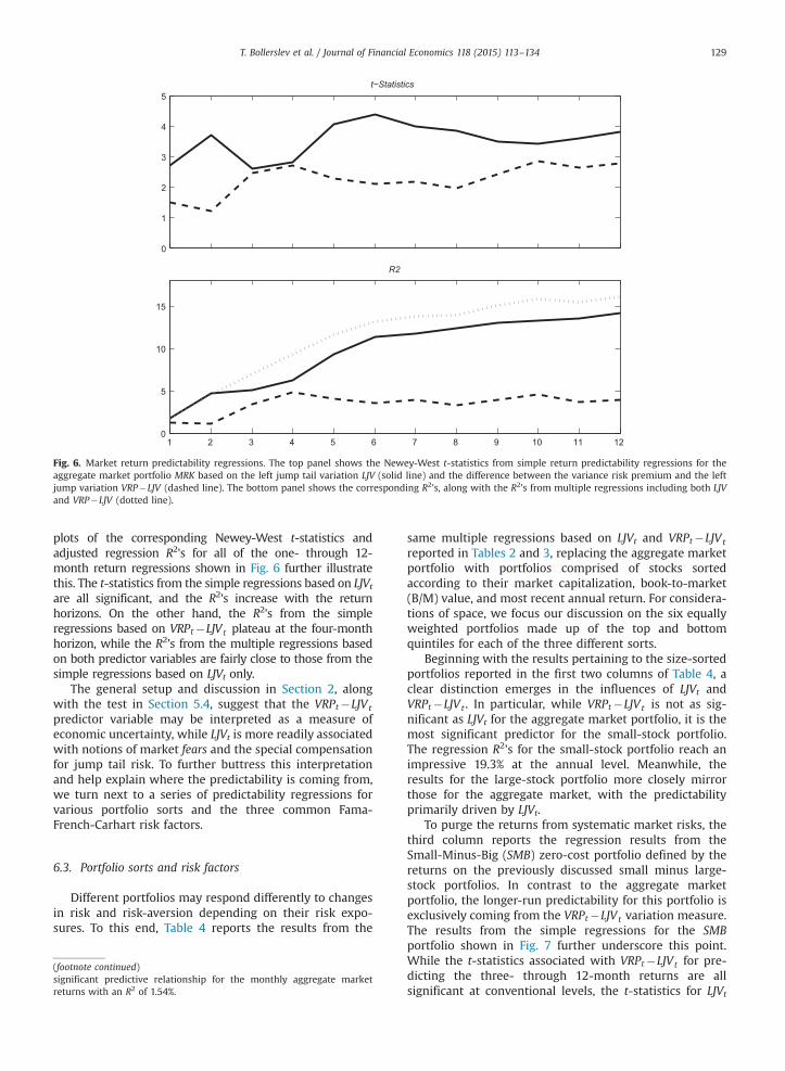
0

1

2

3

4

5t−Statistics

1 2 3 4 5 6 7 8 9 10 11 120

5

10

15

R2

Fig. 6. Market return predictability regressions. The top panel shows the Newey-West t-statistics from simple return predictability regressions for theaggregate market portfolio MRK based on the left jump tail variation LJV (solid line) and the difference between the variance risk premium and the leftjump variation VRP�LJV (dashed line). The bottom panel shows the corresponding R2's, along with the R2's from multiple regressions including both LJVand VRP�LJV (dotted line).


plots of the corresponding Newey-West t-statistics andadjusted regression R2's for all of the one- through 12-month return regressions shown in Fig. 6 further illustratethis. The t-statistics from the simple regressions based on LJVtare all significant, and the R2's increase with the returnhorizons. On the other hand, the R2's from the simpleregressions based on VRPt�LJVt plateau at the four-monthhorizon, while the R2's from the multiple regressions basedon both predictor variables are fairly close to those from thesimple regressions based on LJVt only.

The general setup and discussion in Section 2, alongwith the test in Section 5.4, suggest that the VRPt�LJVt

predictor variable may be interpreted as a measure ofeconomic uncertainty, while LJVt is more readily associatedwith notions of market fears and the special compensationfor jump tail risk. To further buttress this interpretationand help explain where the predictability is coming from,we turn next to a series of predictability regressions forvarious portfolio sorts and the three common Fama-French-Carhart risk factors.

6.3. Portfolio sorts and risk factors

Different portfolios may respond differently to changesin risk and risk-aversion depending on their risk expo-sures. To this end, Table 4 reports the results from the

(footnote continued)significant predictive relationship for the monthly aggregate marketreturns with an R2 of 1.54%.

same multiple regressions based on LJVt and VRPt�LJVt

reported in Tables 2 and 3, replacing the aggregate marketportfolio with portfolios comprised of stocks sortedaccording to their market capitalization, book-to-market(B/M) value, and most recent annual return. For considera-tions of space, we focus our discussion on the six equallyweighted portfolios made up of the top and bottomquintiles for each of the three different sorts.

Beginning with the results pertaining to the size-sortedportfolios reported in the first two columns of Table 4, aclear distinction emerges in the influences of LJVt andVRPt�LJVt . In particular, while VRPt�LJVt is not as sig-nificant as LJVt for the aggregate market portfolio, it is themost significant predictor for the small-stock portfolio.The regression R2's for the small-stock portfolio reach animpressive 19.3% at the annual level. Meanwhile, theresults for the large-stock portfolio more closely mirrorthose for the aggregate market, with the predictabilityprimarily driven by LJVt.

To purge the returns from systematic market risks, thethird column reports the regression results from theSmall-Minus-Big (SMB) zero-cost portfolio defined by thereturns on the previously discussed small minus large-stock portfolios. In contrast to the aggregate marketportfolio, the longer-run predictability for this portfolio isexclusively coming from the VRPt�LJVt variation measure.The results from the simple regressions for the SMBportfolio shown in Fig. 7 further underscore this point.While the t-statistics associated with VRPt�LJVt for pre-dicting the three- through 12-month returns are allsignificant at conventional levels, the t-statistics for LJVt

Table 4Portfolio return predictability regressions.

The table reports the results from one- to 12-month return predictability regressions for size (20% smallest and biggest firms), book-to-market (20% highest and lowest B/M ratios), and momentum (20% top andbottom performers over the past 2–12 months) portfolios, along with the corresponding zero-cost portfolios, analogous to the results for the aggregate market in Tables 2 and 3.

Small Big SMB High Low HML Winners Losers WML

One-month returns

Constant 0.569 0.012 0.557 0.601 �0.180 0.781 1.132 �2.278 3.410(0.980) (0.024) (1.462) (1.126) (�0.368) (2.395) (1.163) (�1.273) (2.369)[0.980] [0.024] [1.462] [1.126] [�0.368] [2.395] [1.163] [�1.273] [2.369]

LJV 0.027 1.179 �1.151 0.260 1.430 �1.169 1.281 4.327 �3.045(0.037) (2.666) (�2.040) (0.463) (3.244) (�2.761) (1.337) (1.606) (�1.189)[0.037] [2.666] [�2.040] [0.463] [3.244] [�2.761] [1.337] [1.606] [�1.189]

VRP�LJV 0.411 0.252 0.159 0.303 0.377 �0.074 0.270 1.817 �1.547(1.744) (1.163) (0.960) (1.321) (1.792) (�0.425) (0.601) (2.060) (�1.692)[1.744] [1.163] [0.960] [1.321] [1.792] [�0.425] [0.601] [2.060] [�1.692]

R2 1.134 2.449 1.780 0.900 3.867 2.551 0.521 4.518 4.156Wald (3.042) (7.795) (7.592) (1.865) (13.73) (8.388) (1.842) (5.066) (2.871)

[3.042] [7.795] [7.592] [1.865] [13.73] [8.388] [1.842] [5.066] [2.871]Three-month returns

Constant 0.546 0.174 0.373 1.459 �0.548 2.008 3.656 �10.59 14.25(0.362) (0.133) (0.381) (1.001) (�0.420) (1.918) (1.448) (�2.019) (3.389)[0.144] [�0.141] [0.451] [0.765] [�0.724] [2.106] [1.054] [�2.003] [3.137]

LJV 2.473 3.248 �0.776 1.366 4.880 �3.514 3.317 19.46 �16.14(1.686) (2.358) (�0.567) (1.089) (3.412) (�2.423) (0.953) (3.534) (�2.409)[0.723] [1.623] [�1.015] [0.278] [2.650] [�2.709] [0.719] [2.559] [�2.041]

VRP�LJV 1.277 0.703 0.574 0.987 0.723 0.264 0.690 6.232 �5.542(2.710) (2.108) (2.311) (2.451) (2.079) (1.032) (1.069) (2.554) (�2.275)[2.428] [1.440] [2.598] [2.166] [1.139] [1.594] [0.756] [2.359] [�2.323]

R2 4.644 6.374 1.531 3.420 9.862 6.477 1.183 19.93 22.78Wald (13.59) (11.11) (7.248) (6.371) (19.39) (11.38) (1.784) (13.63) (6.129)

[13.30] [8.299] [6.886] [6.023] [14.19] [8.387] [1.497] [13.46] [6.701]Six-month returns

Constant �0.339 0.357 �0.696 2.078 �0.522 2.600 5.871 �23.27 29.14(�0.112) (0.127) (�0.386) (0.614) (�0.200) (1.127) (1.222) (�2.085) (3.660)[�0.516] [�0.522] [�0.164] [0.188] [�0.993] [1.367] [0.555] [�2.189] [2.902]

LJV 7.697 7.285 0.412 5.339 9.196 �3.857 9.253 50.34 �41.09(2.663) (3.708) (0.167) (1.772) (4.723) (�1.303) (1.833) (3.669) (�2.587)[0.940] [2.323] [�1.238] [0.991] [2.762] [�2.046] [1.104] [2.420] [�1.894]

VRP�LJV 2.437 0.861 1.576 1.462 0.917 0.545 1.536 7.693 �6.157(2.970) (1.419) (3.474) (1.673) (1.569) (0.969) (1.486) (2.484) (�2.401)[2.004] [0.145] [3.879] [1.337] [�0.093] [1.668] [0.429] [0.771] [�0.831]

R2 12.93 10.33 5.835 6.651 14.34 3.836 3.850 32.93 34.22Wald (17.76) (14.40) (12.38) (3.732) (24.52) (7.408) (6.223) (13.96) (7.439)

[17.76] [12.89] [16.65] [3.732] [21.90] [5.839] [4.639] [15.17] [9.702]Nine-month returns

Constant 0.015 1.107 �1.092 3.275 0.137 3.138 8.196 �27.825 36.021(0.003) (0.240) (�0.368) (0.617) (0.032) (0.877) (1.030) (�1.903) (4.291)

[�0.512] [�0.605] [�0.076] [0.016] [�0.963] [1.155] [0.185] [�1.951] [2.798]

T.Bollerslevet

al./Journal

ofFinancial

Economics

118(2015)

113–134

130

LJV

11.20

9.58

21.62

18.05

511

.48

�3.42

113

.96

63.60

�49

.64

(2.182

)(2.975

)(0.561

)(1.382

)(3.912

)(�

0.80

6)(2.703

)(3.364

)(�

2.86

2)[0.649

][1.759

][�

1.08

3][0.793

][1.956

][�

1.87

5][1.200]

[1.767

][�

1.70

7]VRP�LJV

2.97

61.111

1.86

51.75

51.33

50.42

12.58

18.96

4�6.38

3(2.802

)(1.446

)(2.506

)(1.658

)(1.959

)(0.573

)(2.013

)(2.701

)(�

2.40

2)[1.082

][�

0.12

9][2.586

][0.770

][�

0.14

1][1.485

][0.479

][0.085

][0.093

]R2

16.07

11.01

5.62

08.48

014

.726

1.77

76.116

33.26

29.55

Wald

(15.03

)(8.862

)(8.707

)(2.897

)(16.06

)(6.497

)(10.11

)(13.40

)(8.979

)[10.26

][10.06

][8.404

][2.516

][19.85

][7.204

][9.543

][13.25

][9.221

]12

-mon

threturn

s

Con

stan

t0.87

22.02

0�1.14

85.12

00.81

84.30

310

.76

�28

.06

38.83

(0.171

)(0.339

)(�

0.26

1)(0.812

)(0.145

)(0.924

)(1.029

)(�

1.75

2)(4.902

)[�

0.45

8][�

0.79

9][0.352

][�

0.14

0][�

1.110]

[1.002

][�

0.12

1][�

1.74

2][2.489

]LJV

13.18

11.61

1.57

79.99

513

.86

�3.86

018

.99

68.61

�49

.63

(2.245

)(3.122

)(0.458

)(1.399

)(4.325

)(�

0.67

5)(2.989

)(3.449

)(�

2.84

8)[0.428

][1.547

][�

1.75

4][0.822

][1.744

][�

1.05

4][1.318

][1.421

][�

1.38

7]VRP�LJV

3.71

41.14

72.56

61.45

01.57

1�0.12

12.95

39.31

7�6.36

4(3.222

)(1.382

)(2.817

)(1.341

)(2.012

)(�

0.12

0)(1.928

)(3.089

)(�

2.39

9)[0.967

][�

0.35

4][3.675

][�

0.02

8][�

0.30

0][0.871

][0.061

][�

0.15

9][0.249

]R2

19.31

11.16

7.61

68.10

115

.30

1.53

77.62

930

.30

22.72

Wald

(26.43

)(9.768

)(12.03

)(2.580

)(18.98

)(0.839

)(10.30

)(18.33

)(9.889

)[9.841

][11.89

][16.83

][2.520

][18.13

][1.979

][9.894

][10.99

][6.422

]


are all insignificant. Moreover, the R2's from the multipleregressions that include both VRPt�LJVt and LJVt, shownin the bottom panel of the figure, are very close to the R2'sfrom the simple regressions based on VRPt�LJVt only.

The SMB portfolio has previously been associated withvariables that describe changes in the investment oppor-tunity set (e.g., Petkova, 2006). As such, our finding thatthe predictability of the SMB portfolio is solely driven byVRPt�LJVt is consistent with the idea that this measure ismost directly associated with notions of economic uncer-tainty. Along these lines, a number of studies have alsoargued that smaller firms tend to be more stronglyaffected by credit market conditions than larger firmsand therefore also more susceptible to general economicconditions (see, e.g., Perez-Quiros and Timmermann,2000), thus further helping to explain why VRPt�LJVt isa better predictor for the return on the small-stockportfolio.

The results for the value and growth portfolios alongwith the corresponding High-Minus-Low (HML) book-to-market portfolio reported in the next three columns inTable 4 convey a very different picture. The predictabilitypattern for the low book-to-market portfolio, in particular,fairly closely mirrors that of the aggregate market portfo-lio. On the other hand, the R2's for the HML portfolio inFig. 8 appear to be maximized at the intermediate four-month horizon, with all of the predictability attributable tothe LJVt jump tail variation measure.

The returns on portfolios comprised of growth stockshave previously been related to measures of fundingliquidity risk (e.g., Asness, Moskowitz, and Pedersen,2013). Thus, to the extent that liquidity conditions reflectmarket sentiment, the results in Fig. 8 for the HMLportfolio again indirectly corroborate the interpretationof LJVt as a measure of market fears.

Turning to the results for the momentum portfolios,reported in the last three columns in Table 4, they revealsome very high R2's for the “loser” portfolio made up ofthe stocks that performed the worst over the previous 12months. As shown in Fig. 9, this also translates into veryimpressive R2's for the Winners-Minus-Losers (WML)portfolio in excess of 30% at the six- to eight-monthhorizons. In contrast to the predictability of the SMBportfolio, which appears to be driven solely byVRPt�LJVt , and the predictability of HML, which is solelyattributable to LJVt, both of the two variation measurescontribute to the predictability of the WML portfolio.

The return on momentum portfolios, and “loser” port-folios in particular, have also previously been associatedwith funding liquidity risk (e.g., Pastor and Stambaugh,2003; Korajczyk and Sadka, 2004). The returns on momen-tum portfolios have also been shown to exhibit option-likecharacteristics and be predictable by the “state” of theeconomy and the volatility of the aggregate market (e.g.,Daniel, Jagannathan, and Kim, 2012; Daniel andMoskowitz, 2014), as well as the magnitude of the volati-lity risk premium (e.g., Nagel, 2012; Fan, Imerman, and Dai,2013). Consistent with these earlier findings, the muchstronger predictability for the “loser” and WML portfoliosbased on the decomposition of VRPt reported here againsupport the interpretation of VRPt�LJVt and LJVt as

−4

−2

0

2

4

6SMB t−Statistics

1 2 3 4 5 6 7 8 9 10 11 120

2

4

6

8SMB R2

Fig. 7. SMB return predictability regressions. The top panel shows the Newey-West t-statistics from simple return predictability regressions for the SmallMinus Big (SMB) market capitalization sorted zero-cost portfolio based on the left jump tail variation LJV (solid line) and the difference between thevariance risk premium and the left jump variation VRP�LJV (dashed line). The bottom panel shows the corresponding R2's, along with the R2's frommultiple regressions including both LJV and VRP�LJV (dotted line).

−4

−3

−2

−1

0

1

2HML t−Statistics

1 2 3 4 5 6 7 8 9 10 11 120

2

4

6

8HML R2

Fig. 8. HML return predictability regressions. The top panel shows the Newey-West t-statistics from simple return predictability regressions for the HighMinus Low (HML) book-to-market sorted zero-cost portfolio based on the left jump tail variation LJV (solid line) and the difference between the variancerisk premium and the left jump variation VRP�LJV (dashed line). The bottom panel shows the corresponding R2's, along with the R2's from multipleregressions including both LJV and VRP�LJV (dotted line).


−3.5

−3

−2.5

−2

−1.5

−1

−0.5WML t − Statistics

1 2 3 4 5 6 7 8 9 10 11 120

5

10

15

20

25

30

35WML R2

Fig. 9. WML return predictability regressions. The top panel shows the Newey-West t-statistics from simple return predictability regressions for theWinners Minus Losers (WML) sorted zero-cost portfolio based on the left jump tail variation LJV (solid line) and the difference between the variance riskpremium and the left jump variation VRP�LJV (dashed line). The bottom panel shows the corresponding R2's, along with the R2's frommultiple regressionsincluding both LJV and VRP�LJV (dotted line).


separate proxies for market uncertainty and fears, respec-tively, both of which help predict the momentum returns.

7. Conclusion

The variance risk premium, defined as the differencebetween the actual and risk-neutral expectations of theforward variation of the aggregate market portfolio, isnaturally decomposed into two fundamentally differentsources of market variance risk: “normal” sized price fluctua-tions and jump tail risk. We argue that the part of thevariance risk premium associated with the compensation forleft jump tail risk, in particular, may be seen as a proxy formarket fears. We develop new procedures for empiricallyestimating this component of the variance risk premiumfrom the options surface at a given point in time. Consistentwith the idea that this jump risk component representsseparate state variables that drive the market risk premium,we find that the explanatory power of return predictabilityregressions based on the total variance risk premium, aspreviously reported in the literature, may be significantlyenhanced by including the jump tail risk component as aseparate predictor variable. Our empirical findings corrobo-rate the theoretical equilibrium-based interpretation of thejump tail risk component as being more closely associatedwith changes in risk-aversion, as opposed to changes inmarket risks. The predictability patterns observed for othercommonly studied portfolio sorts and systematic risk factorsconvey a similar message: the predictability of the approxi-mately market-neutral small-minus-big portfolio appears tobe driven solely by the non-jump component, the high-

minus-low book-to-market portfolio is only predicted by thejump risk component, while both components are highlysignificant for predicting the winners-minus-losers portfolioreturns.

Our new jump tail risk measure is obviously related tothe pricing of tail risk in the economy and investors'attitude toward risk more generally. It would be interest-ing to more fully explore these relations, and how the newmeasure relates to other directly observable economicvariables and market-based sentiment indicators. Furtheralong these lines, while the theoretical arguments under-lying our interpretation of the variance risk premiumcomponents and the econometric procedures underlyingtheir separate estimation are both essentially model-free, amore structural-based estimation might afford a deeperunderstanding of the economic mechanisms that drive thetemporal variation in the separate components and helpshed new light on the validity of competing equilibrium-based asset pricing models. We leave further work alongthese lines for future research.

References

Almeida, C., Vicente, J., Guillen, O., 2013. Nonparametric tail risk and stockreturns: predictability and risk premia. Unpublished working paper.Getulio Vargas Foundation, Rio de Janeiro.

Andersen, T.G., Bollerslev, T., Christoffersen, P.C., Diebold, F.X., 2013.Financial risk measurement for financial risk management. In: Con-stantinides, G., Harris, M., Stulz, R. (Eds.), Handbook of the Economicsof Finance, vol. 2b., Elsevier North Holland, Amsterdam, The Nether-lands, pp. 1127–1220.

Andersen, T.G., Fusari, N., Todorov, V., 2015. The risk premia embedded inindex options. Journal of Financial Economics 117, 558–584.

http://refhub.elsevier.com/S0304-405X(15)00126-9/sbref2









Andreou, E., Ghysels, E., 2013. What drives the vix and the volatility riskpremium? Unpublished working paper. University of Cyprus andUniversity of North Carolina Chapel Hill.

Ang, A., Bekaert, G., 2007. Stock return predictability: Is it there? Reviewof Financial Studies 20, 651–707.

Asness, C.S., Moskowitz, T., Pedersen, L.H., 2013. Value and momentumeverywhere. Journal of Finance 68, 929–985.

Baker, M., Wurgler, J., 2006. Investor sentiment and the cross-section ofstock returns. Journal of Finance 61, 1645–1680.

Bakshi, G., Kapadia, N., 2003. Delta-hedge gains and the negative marketvolatility risk premium. Review of Financial Studies 16, 527–566.

Bakshi, G., Madan, D., 2006. A theory of volatility spreads. ManagementScience 52, 1945–1956.

Bali, T.G., Zhou, H., 2015. Risk, uncertainty, and expected returns. Journalof Financial and Quantitative Analysis, forthcoming.

Bansal, R., Shaliastovich, I., 2011. Learning and asset-price jumps. Reviewof Financial Studies 24, 2738–2780.

Bansal, R., Yaron, A., 2004. Risks for the long run: a potential resolution ofasset pricing puzzles. Journal of Finance 59, 1481–1509.

Bates, D.S., 2000. Post-'87 crash fears in the s&p 500 futures optionmarket. Journal of Econometrics 94, 181–238.

Bekaert, G., Engstrom, E., 2010. Asset return dynamics under badenvironment good environment fundamentals. Unpublished workingpaper. Columbia University and U.S. Board of Governors of the FederalReserve System.

Bekaert, G., Hoerova, M., 2014. The vix, the variance premium and stockmarket volatility. Journal of Econometrics 183, 181–192.

Bekaert, G., Hoerova, M., Lo Duca, M., 2013. Risk, uncertainty andmonetary policy. Journal of Monetary Economics 60, 771–788.

Bollerslev, T., Marrone, J., Xu, L., Zhou, H., 2014. Stock return predictabilityand variance risk premia: statistical inference and international evi-dence. Journal of Financial and Quantitative Analysis 49, 633–661.

Bollerslev, T., Sizova, N., Tauchen, G., 2012. Volatility in equilibrium:asymmetries and dynamic dependencies. Review of Finance 16,31–80.

Bollerslev, T., Tauchen, G., Zhou, H., 2009. Expected stock returns andvariance risk premia. Review of Financial Studies 22, 4463–4492.

Bollerslev, T., Todorov, V., 2011a. Estimation of jump tails. Econometrica79, 1727–1783.

Bollerslev, T., Todorov, V., 2011b. Tails, fears and risk premia. Journal ofFinance 66, 2165–2211.

Bollerslev, T., Todorov, V., 2014. Time-varying jump tails. Journal ofEconometrics 183, 168–180.

Bondarenko, O., 2014. Variance trading and market price of variance risk.Journal of Econometrics 180, 81–97.

Bowman, A., Azzalini, A., 1997. Applied Smoothing Techniques for DataAnalysis. Oxford University Press, Oxford, United Kingdom.

Broadie, M., Chernov, M., Johannes, M., 2007. Specification and riskpremiums: the information in s&p 500 futures options. Journal ofFinance 62, 1453–1490.

Campbell, J., Cochrane, J., 1999. By force of habit: a consumption-basedexplanation of aggregate stock market behavior. Journal of PoliticalEconomy 107, 205–251.

Camponovo, L., Scaillet, O., Trojani, F., 2013. Predictive regression androbust hypothesis testing: predictability hidden by anomalous obser-vations. Unpublished working paper. University of Lugano.

Carr, P., Geman, H., Madan, D., Yor, M., 2003. Stochastic volatility for Lévyprocesses. Mathematical Finance 13, 345–382.

Carr, P., Wu, L., 2009. Variance risk premiums. Review of Financial Studies22, 1311–1341.

Chollete, L., Lu, C., 2011. The market premium for dynamic tail risk.Unpublished working paper. University of Stavanger, Norway.

Christoffersen, P., Heston, S., Jacobs, K., 2009. The shape and termstructure of the index option smirk: Why multifactor stochasticvolatility models work so well. Management Science 55, 1914–1932.

Christoffersen, P., Jacobs, K., Ornthanalai, C., 2012. Dynamic jump inten-sities and risk premiums: evidence from s&p 500 returns and options.Journal of Financial Economics 106, 447–472.

Daniel, K., Jagannathan, R., Kim, S., 2012. Tail risk in momentum strategyreturns. NBER Working Paper No. 18169.

Daniel, K., Moskowitz, T., 2014. Momentum crashes. NBER Working PaperNo. 20439.

Davis, R., Mikosch, T., 2009. The extremogram: a correlogram for extremeevents. Bernoulli 15, 977–1009.

Davis, R., Mikosch, T., Cribben, I., 2012. Towards estimating extremalserial dependence via the bootstrapped extremogram. Journal ofEconometrics 170, 142–152.

Drechsler, I., Yaron, A., 2011. What's vol got to do with it? Review ofFinancial Studies 24, 1–45.

Du, D., 2010. General equilibrium pricing of options with habit formationand event risks. Journal of Financial Economics 99, 400–426.

Du, J., Kapadia, N., 2012. Tail and volatility indices from option prices.Unpublished working paper. University of Massachusetts, Amhurst.

Duffie, D., 2001. Dynamic Asset Pricing Theory, third ed. PrincetonUniversity Press, Princeton, NJ.

Duffie, D., Pan, J., Singleton, K., 2000. Transform analysis and asset pricingfor affine jump-diffusions. Econometrica 68, 1343–1376.

Durrleman, V., 2008. Convergence of at-the-money implied volatilities tothe spot volatility. Journal of Applied Probability 45, 542–550.

Eraker, B., 2004. Do stock prices and volatility jump? Reconcilingevidence from spot and option prices. Journal of Finance 59,1367–1403.

Eraker, B., Shaliastovich, I., 2008. An equilibrium guide to designing affinepricing models. Mathematical Finance 18, 519–543.

Eraker, B., Wang, J., 2015. A non-linear dynamic model of the variance riskpremium. Journal of Econometrics, forthcoming.

Fan, J., Imerman, M.B., Dai, W., 2013. What does the volatility riskpremium say about liquidity provision and demand for hedging tailrisk? Unpublished working paper. Princeton University.

Gabaix, X., 2012. Variable rare disasters: an exactly solved framework forten puzzles in macro-finance. Quarterly Journal of Economics 127,645–700.

Hamidieh, K., 2011. Estimating the tail shape parameter from optionprices. Unpublished working paper. California State UniversityFullerton.

Han, B., Zhou, Y., 2011. Variance risk premium and cross-section of stockreturns. Unpublished working paper. University of Texas at Austin.

Hodrick, R.J., 1992. Dividend yields and expected stock returns: alter-native procedures for inference and measurement. Review of Finan-cial Studies 5, 357–368.

Huang, D., Jiang, F., Tu, J., Zhou, G., 2015. Investor sentiment aligned: apowerful predictor of stock returns. Review of Financial Studies 28,791–837.

Kelly, B., Jiang, H., 2014. Tail risk and asset prices. Review of FinancialStudies 27, 2841–2871.

Korajczyk, R., Sadka, R., 2004. Are momentum profits robust to tradingcosts? Journal of Finance 59, 1039–1082.

Li, J., Zinna, G., 2014. Variance components, term structure of variancerisk premia, and expected asset returns. Unpublished working paper.ESSEC Business School.

Mancini, C., 2001. Disentangling the jumps of the diffusion in a geometricjumping Brownian motion. Giornale dell'Istituto Italiano degli AttuariLXIV, 19–47.

Merton, R., 1973. An intertemporal capital asset pricing model. Econo-metrica 41, 867–887.

Nagel, S., 2012. Evaporating liquidity. Review of Financial Studies 25,2005–2039.

Pan, J., 2002. The jump-risk premia implicit in options: evidence from anintegrated time-series study. Journal of Financial Economics 63, 3–50.

Pastor, L., Stambaugh, R.F., 2003. Liquidity risk and expected stockreturns. Journal of Political Economy 111, 642–685.

Perez-Quiros, P., Timmermann, A., 2000. Firm size and cyclical variationsin stock returns. Journal of Finance 55, 1229–1262.

Petkova, R., 2006. Do the Fama–French factors proxy for innovations inpredictive variables? Journal of Finance 61, 581–612.

Protter, P., 2004. Stochastic Integration and Differential Equations, seconded. Springer-Verlag, Berlin.

Ruenzi, S., Weigert, F., 2011. Crash sensitivity and the cross-section ofexpected stock returns. Unpublished working paper. University ofMannheim.

Santa-Clara, P., Yan, S., 2010. Crashes, volatility, and the equity premium:lessons from s&p 500 options. Review of Economics and Statistics 92,435–451.

Schneider, P., 2012. Fear trading. Unpublished working paper. Universityof Lugano.

Schwert, G.W., 2011. Stock volatility during the recent financial crisis.European Financial Management 17, 789–805.

Siriwardane, E., 2013. The probability of rare disasters: estimation andimplications. Unpublished working paper. NYU Stern School ofBusiness.

Todorov, V., 2010. Variance risk premia dynamics: the role of jumps.Review of Financial Studies 23, 345–383.

Vilkov, K., Xiao, Y., 2013. Option-implied information and predictability ofextreme returns. Unpublished working paper. Goethe UniversityFrankfurt.

Wachter, J.A., 2013. Can time-varying risk of rare disasters explainaggregate stock market volatility? Journal of Finance 68, 987–1035.



















































































































Journal of Financial Economics - Duke...

Documents

Transcript of Journal of Financial Economics - Duke...