Journal of Financial Economics - Duke...
27
Journal of Financial Economics 120 (2016) 464–490 Contents lists available at ScienceDirect Journal of Financial Economics journal homepage: www.elsevier.com/locate/finec Roughing up beta: Continuous versus discontinuous betas and the cross section of expected stock returns Tim Bollerslev a,b,c , Sophia Zhengzi Li d,∗ , Viktor Todorov e a Department of Economics, Duke University, Durham, NC 27708, USA b National Bureau of Economic Research, USA c CREATES, Denmark d Department of Finance, Eli Broad College of Business, Michigan State University, East Lansing, MI 48824, USA e Department of Finance, Kellogg School of Management, Northwestern University, Evanston, IL 60208, USA a r t i c l e i n f o Article history: Received 30 March 2015 Revised 6 August 2015 Accepted 10 August 2015 Available online 24 February 2016 JEL Classification: C13 C14 G11 G12 Keywords: Market price risks Jump betas High-frequency data Cross-sectional return variation a b s t r a c t We investigate how individual equity prices respond to continuous and jumpy market price moves and how these different market price risks, or betas, are priced in the cross section of expected stock returns. Based on a novel high-frequency data set of almost 1,000 stocks over two decades, we find that the two rough betas associated with intraday discontinu- ous and overnight returns entail significant risk premiums, while the intraday continuous beta does not. These higher risk premiums for the discontinuous and overnight market betas remain significant after controlling for a long list of other firm characteristics and explanatory variables. © 2016 Published by Elsevier B.V. An earlier version of the paper by Tim Bollerslev and Sophia Zhengzi Li was circulated under the title “Roughing up the CAPM: Jump betas and the cross section of expected stock returns.” We are grateful to Bill Schw- ert (the editor), and an anonymous referee for numerous helpful sugges- tions, which greatly improved the paper. We would also like to thank Turan Bali, Jia Li, Andrew Patton, Mark Schroder, and George Tauchen, along with seminar participants at several universities, financial insti- tutions, and conferences for their helpful comments. The research was partly funded by a grant from the National Science Foundation (SES- 0957330) to the National Bureau of Economic Research. Bollerslev and Li also gratefully acknowledge support from CREATES funded by the Dan- ish National Research Foundation (DNRF78) and the 2012 Morgan Stanley Prize for Excellence in Financial Markets, respectively. ∗ Corresponding author. Tel: +1 517 353 3115; fax: +1 517 884 3718. E-mail addresses: [email protected] (T. Bollerslev), lizhengzi@broad. msu.edu (S.Z. Li), [email protected] (V. Todorov). 1. Introduction The idea that only systematic market price risk should be priced represents one of the cornerstones of finance. Even though numerous studies over the past half-century have called into question the ability of the capital asset pricing model (CAPM) to fully explain the cross section of expected stock returns, the beta of an asset arguably re- mains the most commonly used systematic risk measure in financial practice. Early work by Fama, Fisher, Jensen, and Roll (1969) and Blume (1970) generally supports the CAPM. Subsequent prominent empirical studies that call into question the explanatory power of market betas for satisfactorily explaining the cross section of expected re- turns include Basu (1977, 1983), Roll (1977), Banz (1981), Stattman (1983), Rosenberg, Reid, and Lanstein (1985), Bhandari (1988), and Fama and French (1992). Meanwhile, http://dx.doi.org/10.1016/j.jfineco.2016.02.001 S0304-405X(16)30001-0/© 2016 Published by Elsevier B.V.
Transcript of Journal of Financial Economics - Duke...

Journal of Financial Economics 120 (2016) 464–490
Contents lists available at ScienceDirect
Journal of Financial Economics
journal homepage: www.elsevier.com/locate/finec
Roughing up beta: Continuous versus discontinuous betas and
the cross section of expected stock returns
�
Tim Bollerslev
a , b , c , Sophia Zhengzi Li d , ∗, Viktor Todorov
e
a Department of Economics, Duke University, Durham, NC 27708, USA b National Bureau of Economic Research, USA c CREATES, Denmark d Department of Finance, Eli Broad College of Business, Michigan State University, East Lansing, MI 48824, USA e Department of Finance, Kellogg School of Management, Northwestern University, Evanston, IL 60208, USA
a r t i c l e i n f o
Article history:
Received 30 March 2015
Revised 6 August 2015
Accepted 10 August 2015
Available online 24 February 2016
JEL Classification:
C13
C14
G11
G12
Keywords:
Market price risks
Jump betas
High-frequency data
Cross-sectional return variation
a b s t r a c t
We investigate how individual equity prices respond to continuous and jumpy market price
moves and how these different market price risks, or betas, are priced in the cross section
of expected stock returns. Based on a novel high-frequency data set of almost 1,0 0 0 stocks
over two decades, we find that the two rough betas associated with intraday discontinu-
ous and overnight returns entail significant risk premiums, while the intraday continuous
beta does not. These higher risk premiums for the discontinuous and overnight market
betas remain significant after controlling for a long list of other firm characteristics and
explanatory variables.
© 2016 Published by Elsevier B.V.
� An earlier version of the paper by Tim Bollerslev and Sophia Zhengzi
Li was circulated under the title “Roughing up the CAPM: Jump betas and
the cross section of expected stock returns.” We are grateful to Bill Schw-
ert (the editor), and an anonymous referee for numerous helpful sugges-
tions, which greatly improved the paper. We would also like to thank
Turan Bali, Jia Li, Andrew Patton, Mark Schroder, and George Tauchen,
along with seminar participants at several universities, financial insti-
tutions, and conferences for their helpful comments. The research was
partly funded by a grant from the National Science Foundation (SES-
0957330) to the National Bureau of Economic Research. Bollerslev and Li
also gratefully acknowledge support from CREATES funded by the Dan-
ish National Research Foundation (DNRF78) and the 2012 Morgan Stanley
Prize for Excellence in Financial Markets, respectively. ∗ Corresponding author. Tel: +1 517 353 3115; fax: +1 517 884 3718.
E-mail addresses: [email protected] (T. Bollerslev), lizhengzi@broad.
msu.edu (S.Z. Li), [email protected] (V. Todorov).
http://dx.doi.org/10.1016/j.jfineco.2016.02.001
S0304-405X(16)30 0 01-0/© 2016 Published by Elsevier B.V.
1. Introduction
The idea that only systematic market price risk should
be priced represents one of the cornerstones of finance.
Even though numerous studies over the past half-century
have called into question the ability of the capital asset
pricing model (CAPM) to fully explain the cross section of
expected stock returns, the beta of an asset arguably re-
mains the most commonly used systematic risk measure
in financial practice. Early work by Fama, Fisher, Jensen,
and Roll (1969) and Blume (1970) generally supports the
CAPM. Subsequent prominent empirical studies that call
into question the explanatory power of market betas for
satisfactorily explaining the cross section of expected re-
turns include Basu (1977, 1983) , Roll (1977) , Banz (1981) ,
Stattman (1983) , Rosenberg, Reid, and Lanstein (1985) ,
Bhandari (1988) , and Fama and French (1992) . Meanwhile,

T. Bollerslev et al. / Journal of Financial Economics 120 (2016) 464–490 465
more recent empirical evidence pertaining to the equity
risk premium and the pricing of risk at the aggregate mar-
ket level suggests that the expected return variation asso-
ciated with discontinuous price moves, or jumps, is priced
higher than the expected continuous price variation. 1
Set against this background, we propose a general pric-
ing framework involving three separate market betas: a
continuous beta reflecting smooth intraday co-movements
with the market and two rough betas associated with in-
traday price discontinuities, or jumps, during the active
part of the trading day and the overnight close-to-open re-
turn, respectively. The seminal paper by Merton (1976) hy-
pothesizes that jump risks for individual stocks are likely
to be nonsystematic. Empirical evidence of increased cross-
asset correlations for higher (in an absolute sense) re-
turns shown in Ang and Chen (2002) , among many oth-
ers, indirectly suggests nonzero systematic jump risk, as
does the downside risk asset pricing model recently ex-
plored by Lettau, Maggiori, and Weber (2014) . Consistent
with the idea that investors view intraday smooth and
that easier to hedge price moves differently from intra-
day rough and day-to-day overnight price changes, we find
that the risk premiums associated with the two jump be-
tas are both statistically significant and indistinguishable,
while the continuous beta does not appear to be priced in
the cross-section. 2
The theoretical framework motivating our empirical in-
vestigations and the separate cross-sectional pricing of
continuous and discontinuous market price risks is very
general and merely assumes the existence of a generic
pricing kernel along the lines of Duffie, Pan, and Single-
ton (20 0 0) . Importantly, we make no explicit assumptions
about the pricing of other nonmarket price risks. As such,
our setup includes the popular long-run risk model of
Bansal and Yaron (2004) , the habit persistence model of
Campbell and Cochrane (1999) , and the rare disaster model
of Gabaix (2012) , as special cases obtained by further re-
stricting the functional form of the pricing kernel, the set
of other priced risk factors, and the connections with fun-
damentals.
The statistical theory underlying our estimation of
the separate betas builds on recent advances in financial
econometrics related to the use of high-frequency intraday
data and so-called realized volatilities. Bollerslev and
Zhang (2003) , Barndorff-Nielsen and Shephard (2004a ),
and Andersen, Bollerslev, Diebold, and Wu (2005 , 2006) ,
in particular, have explored the use of high-frequency data
and the asymptotic notion of increasingly finer sampled
returns over fixed time intervals for more accurately esti-
mating realized betas. In contrast to these earlier studies,
1 Empirical evidence based on aggregate equity index options in sup-
port of this hypothesis is presented by Pan (2002) , Eraker, Johannes, and
Polson (2003) , Bollerslev and Todorov (2011) , and Gabaix (2012) , among
others. 2 Optimally managing market diffusive and jump price risks require
the use of different hedging tools and derivative instruments; see, e.g.,
the theoretical analysis in Liu, Longstaff, and Pan (2003a , 2003b) . The
increased availability of short-maturity out-of-the-money options, which
provide a particular convenient tool for managing jump tail risk, also
directly speaks to the practical importance of separately accounting for
these different types of risks.
which do not differentiate among different types of market
price moves, we rely on the theory originally developed
by Todorov and Bollerslev (2010) for explicitly estimat-
ing separate continuous and discontinuous betas for the
open-to-close active part of the trading day, together with
overnight betas for the close-to-open returns. 3
Our actual empirical investigations are based on a novel
high-frequency data set of all the 985 stocks included in
the Standard & Poor’s (S&P) 500 index over the 1993–2010
sample period. We begin by estimating the three separate
betas as well as a standard CAPM regression-based beta for
each of the individual stocks on a rolling one-year basis.
Consistent with the basic tenets of the simple CAPM, we
find that sorting the stocks in our sample on the basis of
their betas results in a positive return differential between
the high- and low-beta quintile portfolios for all of the four
different beta estimates. However, even though all of the
return differentials are large numerically, the difference in
the monthly returns between the high- and low-beta port-
folios constructed on the basis of the standard CAPM betas
is not significantly different from zero at conventional lev-
els. Similarly, sorting by our continuous beta estimates, the
monthly long–short excess return for the high- minus low-
beta quintile portfolios is not significantly different from
zero. Sorting stocks on the basis of their discontinuous
and overnight betas, as well as their relative betas defined
by the difference between either of the two jump betas
and the standard beta, results in significantly positive risk-
adjusted returns on the high–low portfolios. 4 More impor-
tant from a practical perspective, we show that these same
significant contemporaneous return differentials carry over
to a predictive setting, in which we compare the subse-
quent realized monthly returns of the quintile portfolios
based on grouping the stocks according to their past rolling
one-year beta estimates.
These predictive return differentials associated with the
discontinuous and overnight betas remain statistically sig-
nificant in double portfolio sorts designed to control for a
number of other firm characteristics and risk factors pre-
viously associated with the cross section of expected re-
turns, including firm size, book-to-market ratio, momen-
tum, short-term reversal, idiosyncratic volatility, maximum
daily return, illiquidity, and various measures of skewness
and kurtosis. Standard predictive Fama–MacBeth regres-
sions further corroborate the idea that only rough mar-
ket risks are priced. While the estimated risk premiums
associated with the intraday discontinuous and overnight
betas are both significant after simultaneously controlling
for a long list of firm characteristics and other risk factors,
the estimated risk premium associated with the continu-
ous beta is not.
Our main empirical findings rely on a relatively coarse
75-minute intraday sampling frequency for the one-year
3 Branch and Ma (2012) , Cliff, Cooper, and Gulen (2008) , and Berkman,
Koch, Tuttle, and Zhang (2012) also show distinctly different return pat-
terns during trading and non-trading hours. 4 As discussed further in Section 5.2 , this contrasts with the recent re-
sults in Frazzini and Pedersen (2014) , who report an almost flat security
market line and highly significant positive CAPM alphas for portfolios bet-
ting against beta.

466 T. Bollerslev et al. / Journal of Financial Economics 120 (2016) 464–490
rolling continuous and jump beta estimation, as a way to
guard against nonsynchronous trading effects and other
market microstructure complications that arise at the high-
est intraday sampling frequency. However, our results re-
main robust to the use of other sampling frequencies and
inference procedures for the estimation of the betas. Simi-
larly, while our main cross-sectional regressions are based
on a standard one-year estimation and subsequent one-
month holding period, even stronger results hold true
for other estimation windows and return holding periods.
Also, while some of the jumps that occur at the aggregate
market level are naturally associated with news about the
economy, our results remain robust to the exclusion of sev-
eral important macroeconomic news announcement days. 5
The idea of allowing for time-varying market betas to
help explain the cross section of expected stock returns is
related to the large literature on testing conditional ver-
sions of the CAPM. 6 In contrast to this literature, our em-
pirical investigations should not be interpreted as a test
of the conditional CAPM per se. Instead, motivated by our
general pricing framework, we simply show that market
risks with different degrees of jumpiness, as determined
by our high-frequency-based estimates of the time-varying
continuous and jump betas, are priced differently and that
these cross-sectional differences in the returns cannot be
explained by other firm characteristics or commonly used
risk factors. We are not arguing that market risk is the only
source of priced risk in the cross section.
Our work is also related to, but fundamentally differ-
ent from, several recent studies that have examined how
jump risk can help explain the cross section of expected
stock returns. Jiang and Yao (2013) argue that the size pre-
mium, the liquidity premium and, to a lesser extent, the
value premium are all realized in the cross-sectional dif-
ferences of jump returns. Cremers, Halling, and Weinbaum
(2015) show that market expectations of aggregate jump
risk implied from options prices are useful for explaining
the cross-sectional variation in expected returns, and Yan
(2011) shows that expected stock returns are negatively re-
lated to average jump sizes. Our work differs from these
studies in at least two important dimensions. First, we fo-
cus explicitly on systematic jump risk, as measured by the
exposure to nondiversifiable market-wide jumps and the
two rough betas. Second, our use of high-frequency data to
directly identify the intraday jumps and estimate the betas
sets our study apart from other research inferring the jump
risk from daily or lower-frequency data.
Our cross-sectional pricing results also complement re-
cent time series estimates of the equity risk premium re-
5 Initial studies showing large changes in high-frequency intraday
returns in response to macroeconomic news announcements include
Fleming and Remolona (1999) and Andersen, Bollerslev, Diebold, and Vega
(20 03 , 20 07b) . 6 Early contributions to this literature include Ferson, Kandel, and
Stambaugh (1987) , Bollerslev, Engle, and Wooldridge (1988) , and Harvey
(1989) , among others, along with more recent cross-sectionally oriented
studies by Jagannathan and Wang (1996) and Lettau and Ludvigson
(2001) . Bali, Engle, and Tang (2015) have also recently argued that gener-
alized autoregressive conditional heteroskedasticity (GARCH)-based time-
varying conditional betas help explain the cross-sectional variation in ex-
pected stock returns.
ported in Bollerslev and Todorov (2011) and Gabaix (2012) ,
among others, which suggest that a large portion of the ag-
gregate equity premium and the temporal variation therein
could be attributable to jump tail risk. In line with these
findings for the aggregate market, the two rough betas
associated with intraday jumps and day-to-day overnight
price changes directly reflect the individual stocks’ system-
atic response to jump risk and, in turn, receive the largest
compensation in the cross section. Intuitively, large stock
price movements likely provide better signals about true
changes in fundamentals and equity valuations than do
smaller within-day price fluctuations, which could simply
represent noise in the price formation process.
The remainder of the paper is organized as follows.
Section 2 formally defines the different betas and the
theory underlying their separate pricing within a con-
ventional equilibrium-based asset pricing framework. The
statistical procedures used for estimating the separate
betas are discussed in Section 3 . Section 4 describes the
high-frequency data that we use to estimate the be-
tas and the control variables employed in our empirical
investigations. Section 5 presents our initial empirical ev-
idence pertaining to various portfolio sorts. Section 6 dis-
cusses the results from the predictive firm-level cross-
sectional pricing regressions and the estimates of the risk
premiums for the different betas. Section 7 presents a se-
ries of robustness checks related to the intraday sampling
frequency used in the estimation of the betas, possible
nonsynchronous trading effects, errors-in-variables in the
cross-sectional pricing regressions, the length of the beta
estimation and return holding periods, and the influence
of specific macroeconomic news announcements. Section 8
concludes. Appendix details the high-frequency data clean-
ing rules and the definitions of the explanatory variables
used in the analysis.
2. Continuous and discontinuous market risk pricing
Our theoretical framework motivating the different be-
tas and the separate pricing of continuous and discontin-
uous market price risks is very general and merely relies
on no-arbitrage and the existence of a pricing kernel. By
the same token, we do not provide explicit equilibrium-
based expressions for the separate risk premiums. Doing
so would require additional assumptions beyond the ones
necessary for simply separating the continuous and discon-
tinuous market risk premiums and the corresponding mar-
ket betas.
To set out the notation, let the price of the aggregate
market portfolio be denoted by P (0) t , with the correspond-
ing logarithmic price denoted by lowercase p (0) t ≡ log P (0)
t .
We assume the following general dynamic representation
for the instantaneous return on the market:
d p (0) t = α(0)
t d t + σt d W t +
∫ R
x μ(d t, d x ) , (1)
where W t denotes a Brownian motion describing con-
tinuous Gaussian, or smooth, market price shocks with
diffusive volatility σ t and
˜ μ is a (compensated) jump
counting measure accounting for discontinuous, or rough,

T. Bollerslev et al. / Journal of Financial Economics 120 (2016) 464–490 467
market price moves. 7 The drift term α(0) t is explicitly re-
lated to the pricing of these separate market risks.
We denote the cross section of individual stock prices
by P (i ) t , i = 1 , . . . , n . In parallel to the representation for the
market portfolio, we assume that the instantaneous loga-
rithmic price process, p (i ) t ≡ log P (i )
t , for each of the n indi-
vidual stocks could be expressed as
dp (i ) t = α(i )
t d t + β(c,i ) t σ (i )
t d W t +
∫ R
β(d,i ) t x μ(d t, d x )
+
˜ σ (i ) t d W
(i ) t +
∫ R
x μ(i ) (d t, d x ) , (2)
where the W
(i ) t Brownian motion is orthogonal to W t ,
but possibly correlated with W
( j) t for i � = j , and the
μ( i ) jump measure is orthogonal to μ in the sense that
μ({ t} , R ) μ(i ) ({ t} , R
p ) = 0 for every t , so that μ( i ) counts
only firm-specific jumps occurring at times when the mar-
ket does not jump. By explicitly allowing the individual
loadings, or betas, associated with the market diffusive
and jump risks to be time-varying, this decomposition of
the continuous and discontinuous martingale parts of as-
set i ’s return into separate components directly related to
their market counterparts and orthogonal components (in
a martingale sense) is extremely general. For the diffusive
part, this entails no assumptions and follows merely from
the partition of a correlated bivariate Brownian motion
into its orthogonal components (see, e.g., Theorem 2.1.2
in Jacod and Protter, 2012 ). For the discontinuous part,
the decomposition implicitly assumes that the relation be-
tween the systematic jumps in the asset and the market
index, while time-varying, does not depend on the size of
the jumps. 8 This type of restriction is arguably unavoid-
able. By their very nature, systematic jumps are relatively
rare, and as such it is not feasible to identify different jump
betas for different jump sizes, let alone identify the small
jumps in the first place. This assumption also maps directly
into the way in which we empirically estimate jump betas
for each of the individual stocks based solely on the large-
size jumps.
To analyze the pricing of continuous and discontinuous
market price risks, we follow standard practice in the asset
pricing literature and assume the existence of an economy-
wide pricing kernel of the form (see, e.g., Duffie, Pan, and
Singleton, 20 0 0 )
M t = e −∫ t
0 r s ds E (
−∫ t
0
λs dW s
+
∫ t
0
∫ R
(κ(s, x ) − 1) μ(d s, d x )
)M
′ t , (3)
7 The compensated jump counting measure is formally related to the
actual counting measure μ for the jumps in P (0) by the expression ˜ μ(d t, d x ) ≡ μ(d t, d x ) − dt ⊗ νt (dx ) , where νt ( dx ) denotes the (possibly
time-varying) intensity of the jumps, thus rendering the ˜ μ measure a
martingale. 8 Formally, let s denote a time when the market jumps and �p (0)
s � = 0 .
The representation in Eq. (2) then implies that �p (i ) s / �p (0)
s = β(d,i ) s , al-
lowing the jump beta to vary with the time s but not the actual size of
the jump.
Y
where r t denotes the instantaneous risk-free interest rate
and E(·) refers to the stochastic exponential. 9 The càdlàg
λt process and the predictable κ( t, x ) function account for
the pricing of diffusive and jump market price risks, re-
spectively. The last term, M
′ t , encapsulates the pricing of all
other (orthogonalized to the market price risks) systematic
risk factors. In parallel to the first part of the expression
for M t , we assume that this additional part of the pricing
kernel takes the form,
M
′ t = E
(−
∫ t
0
λ′ s dW
′ s +
∫ t
0
∫ R
(κ ′ (s, x ) − 1) μ′ (ds, dx )
),
(4)
where the W
′ t Brownian motion is orthogonal to W t and
the two jump measures μ and μ′ are orthogonal in the
sense that μ({ t} , R ) μ′ ({ t} , R
p ) = 0 for every t , so that the
respective jumps never arrive at the exact same instant.
The pricing kernel jointly defined by Eqs. (3) and (4) en-
compasses almost all parametric asset pricing models hith-
erto analyzed in the literature as special cases.
To help fix ideas, consider the case of a static
pure-endowment economy, with independent and iden-
tically distributed consumption growth and a represen-
tative agent with Epstein–Zin preferences. In this basic
consumption-based CAPM (CCAPM) setup, the dynamics of
the pricing kernel are driven solely by consumption. As-
suming that the market portfolio represents a claim on
total consumption, it therefore follows that M
′ t ≡ 1 , result-
ing in a pricing kernel that solely depends on the diffu-
sive Gaussian and discontinuous market price shocks. This
same analysis continues to hold true for a representative
agent with habit persistence as in Campbell and Cochrane
(1999) , the only difference being that in this situation the
prices of the diffusive and jump market risks are time-
varying due to the temporal variation in the degree of
risk-aversion of the representative agent. In general, tem-
poral variation in the investment opportunity set, as in the
intertemporal CAPM (ICAPM) of Merton (1973) , could in-
duce additional sources of priced risks. Leading examples
of other state variables that could affect the pricing kernel
include the conditional mean and volatility of consumption
growth as in Bansal and Yaron (2004) and the time-varying
probability of a disaster as in Gabaix (2012) and Wachter
(2013) . 10 However, given our primary focus on the pricing
of market price risk, we purposely do not take a stand on
what these other risk factors could be, instead simply rele-
gating their influence over and above what can be spanned
by the market to the additional M
′ t part of the pricing
kernel.
The pricing kernel in Eq. (3) has also been widely used
in the literature on derivatives pricing. For reasons of an-
alytical tractability, in that literature the common assump-
tions are that λt is proportional to the market diffusive
9 Formally, for some arbitrary process Z , E(Z) is defined by the solu-
tion to the stochastic differential equation dY Y −
= dZ, with initial condition
0 = 1 . 10 In models involving nonfinancial wealth, so that the market portfo-
lio and the total wealth portfolio are not perfect substitutes, additional
sources of risks also naturally arise.

468 T. Bollerslev et al. / Journal of Financial Economics 120 (2016) 464–490
14 This contrast with the derivations in Longstaff (1989) , who shows
how temporally aggregating the simple continuous-time CAPM results in
a multifactor model, and the more recent paper by Corradi, Distaso, and
Fernandes (2013) that delivers conditional time-varying alphas and be-
volatility σ t , the jump intensity νt ( dx ) is affine in σ 2 t , and
the price of jump risk κ( t, x ) is time-invariant. See, e.g.,
Duffie, Pan, and Singleton (20 0 0) , who show that these as-
sumptions greatly facilitate the calculation of closed-form
derivatives pricing formulas. These same assumptions also
imply that the equity risk premium should be proportional
to the variance of the aggregate market portfolio. 11
In general, it follows readily by a standard change-of-
measure (see, e.g., Jacod and Shiryaev, 2002 ) that without
any additional restrictions on the pricing kernel defined by
Eqs. (3) and (4) , the instantaneous market risk premium
must satisfy
α(0) t − r t − δ(0)
t − q (0) t = γ c
t + γ d t , (5)
where δ(0) t refers to the dividend yield on the market port-
folio, and the compensation for continuous and discontin-
uous market price risks are determined by
γ c t ≡ σt λt , and γ d
t ≡∫ R
xκ(t, x ) νt (dx ) , (6)
respectively, and q (0) t represents a standard convexity ad-
justment term. 12 Because the compensation stemming
from M
′ t is orthogonal to the compensation for market
price risk, this expression for α(0) t depends only on the first
part of the pricing kernel.
For the individual assets, even though the W
(i ) t and μ( i )
diffusive and jump risks are orthogonal to the correspond-
ing market diffusive and jump risk components, they could
nevertheless be priced in the cross section as they could be
correlated with the W
′ t and μ′ risks that appear in the M
′ t
part of the pricing kernel. Denoting the part of the instan-
taneous risk premium for asset i arising from this separate
pricing of W
(i ) t and μ( i ) by ˜ α(i )
t , it follows again by stan-
dard arguments that
α(i ) t − r t − δ(i )
t − q (i ) t = β(c,i )
t γ c t + β(d,i )
t γ d t +
α(i ) t , (7)
where δ(i ) t refers to the dividend yield of asset i and q (i )
t
denotes a standard convexity adjustment term stemming
from the pricing of market price risks. 13
If ˜ α(i ) t ≡ 0 , as would be implied by M
′ t ≡ 1 , and if β(c,i )
t
and β(d,i ) t were also the same, the expression in Eq. (7)
trivially reduces to a simple continuous-time one-factor
CAPM that linearly relates the instantaneous return on
stock i to its single beta. The restriction that β(c,i ) t = β(d,i )
t
implies that the asset responds the same to market diffu-
sive and jump price increments or, intuitively, that the as-
set and the market co-move the same during normal times
and periods of extreme market moves. If β(c,i ) t and β(d,i )
t
differ, em pirical evidence for which is provided below, the
cross-sectional variation in the continuous and jump be-
tas could be used to identify their separate pricing. Impor-
tantly, this remains true in the presence of other priced
risk factors, when
˜ α(i ) is not necessarily equal to zero.
t11 This simple relation has been extensively investigated in the empirical
asset pricing literature. See, e.g., Bollerslev, Sizova, and Tauchen (2012)
and the many additional references therein. 12 The q (0)
t term is formally given by 1 2 σ 2
t +
∫ R
( e x − 1 − x ) νt (dx ) .
13 In parallel to the expression for q (0) t above, q (i )
t =
1 2
(β(c,i )
t σt
)2 + ∫ R
(e β
(d,i ) t x − 1 − β(d,i )
t x
)νt (dx ) .
In practice, the returns on the assets have to be mea-
sured over some nontrivial time interval, say, h > 0. Let
r (i ) t ,t + h ≡ p (i )
t+ h − p (i ) t denote the corresponding logarithmic
return on asset i . For empirical tractability, assume that the
betas remain constant over that same (short) time interval.
The integrated conditional risk premium for asset i could
then be expressed as
E t
(r (i )
t ,t + h −∫ t+ h
t
(r s + δ(i ) s + q (i )
s ) ds
)
= β(c,i ) t E t
(∫ t+ h
t
γ c s ds
)+ β(d,i )
t E t
(∫ t+ h
t
γ d s ds
)
+ E t
(∫ t+ h
t
˜ α(i ) s ds
). (8)
This expression for the discrete-time expected excess re-
turn maintains the same two-beta structure as the expres-
sion for the instantaneous risk premiums in Eq. (7) . 14 It
clearly highlights how the pricing of continuous and dis-
continuous market price risks could manifest differently in
the cross section of expected stock returns and, in turn,
how separately estimating β(c,i ) t and β(d,i )
t could allow for
more accurate empirical predictions of the actual realized
returns.
3. Continuous and discontinuous beta estimation
The decompositions of the prices for the market and
each of the individual assets into separate diffusive and
jump components that formally underly β(c,i ) t and β(d,i )
t in
Eqs. (1) and (2) are not directly observable. Instead, the
different continuous-time price components and, in turn,
the betas have to be deduced from observed discrete-time
prices and returns.
To this end, we assume that high-frequency intraday
prices are available at time grids of length 1/ n over the
active intraday part of the trading day [ t, t + 1) . For no-
tational simplicity, we denote the corresponding logarith-
mic discrete-time return on the market over the τ th in-
traday time interval by r (0) t: τ ≡ p (0)
t+ τ/n − p (0) t+(τ−1) /n
, with the
τ th intraday return for asset i defined accordingly as r (i ) t: τ ≡
p (i ) t+ τ/n − p (i )
t+(τ−1) /n . The theory underlying our estimation
is formally based on the notion of fill-in asymptotics and
n → ∞ , or ever finer sampled high-frequency returns. 15 To
allow for reliable estimation, we further assume that the
tas within a similar setting. Instead, our derivation is based on a general
continuous-time jump-diffusion representation and arrives at a consistent
two-factor discrete-time pricing relation under the assumption that the
separate jump and diffusive betas remain constant over the (short) return
horizons. 15 Host of practical market microstructure complications invariably pre-
vents us from sampling too finely. To assess the sensitive of our results to
the specific choice of n , we experiment with the use of several different
sampling schemes, including ones in which n ( i ) varies across stocks.

T. Bollerslev et al. / Journal of Financial Economics 120 (2016) 464–490 469
r (0) s : τ ) 2
) τ }
18 The basic idea of relying on higher order powers of returns to isolate
the jump component of the price has previously been used in many other
betas stay constant over multi-day time-intervals of length
l > 1. 16
To begin, consider the estimation of the continuous be-
tas. To convey the intuition, suppose that neither the mar-
ket nor stock i jumps, so that μ ≡ 0 and μ( i ) ≡ 0 almost
surely. For simplicity, suppose also that the drift terms in
Eqs. (5) and (7) are both equal to zero, so that
r (i ) s : τ = β(i,c)
t r (0) s : τ +
r (i ) s : τ , where ˜ r (i )
s : τ ≡∫ s + τ/n
s +(τ−1) /n
σ (i ) u dW
(i ) u ,
(9)
for any s ∈ [ t − l, t] . Thus, in this situation, the contin-
uous beta could simply be estimated by an ordinary
least squares (OLS) regression of the discrete-time high-
frequency returns for stock i on the high-frequency returns
for the market. Using a standard polarization of the covari-
ance term, the resulting regression coefficient can be ex-
pressed as ∑ t−1 s = t−l
∑
τ r (i ) s : τ r (0)
s : τ∑ t−1 s = t−l
∑
τ (r (0) s : τ ) 2
≡∑ t−1
s = t−l
∑
τ
[(r (i )
s : τ + r (0) s : τ ) 2 − (r (i )
s : τ − r (0) s : τ ) 2
]4
∑ t−1 s = t−l
∑
τ (r (0) s : τ ) 2
. (10)
In general, the market and stock i could both jump over
the [ t − l, t] time interval, and the drift terms are not iden-
tically equal to zero. Meanwhile, it follows readily by stan-
dard arguments that for n → ∞ , the impact of the drift
terms are asymptotically negligible. However, to allow for
the possible occurrence of jumps, the simple estimator de-
fined above needs to be appropriately modified by remov-
ing the discontinuous components. The polarization of the
covariance provides a particularly convenient way of doing
so by expressing the estimator in terms of sample portfolio
variances. In particular, as shown by Todorov and Boller-
slev (2010) , the truncation-based estimator defined by
β(c,i ) t =
∑ t−1 s = t−l
∑ n τ=1
[ (r (i )
s : τ + r (0) s : τ ) 2 1 {| r (i )
s : τ + r (0) s : τ |≤k (i +0)
s,τ } − (r (i ) s : τ −
4
∑ t−1 s = t−l
∑ n τ=1 (r (0)
s : τ ) 2 1 {| r (0) s : τ |≤k (0
s,
consistently estimates the continuous beta for n → ∞ un-
der very general conditions. 17
Next, consider the estimation of the discontinuous beta.
Assuming that β(d,i ) t is positive, it follows that for any
s ∈ [ t − l, t] such that �p (0) s � = 0 , the discontinuous beta is
uniquely identified by
β(d,i ) t ≡
√ √ √ √
(�p (i )
s �p (0) s
)2
(�p (0)
s
)4 . (12)
16 Due to the relatively rare nature of jumps, in our main empirical re-
sults, we base the estimation on a full year. However, we also experiment
with the use of shorter estimation periods, if anything, resulting in even
stronger results and more pronounced patterns. 17 In our empirical analysis, we follow Bollerslev, Todorov, and Li (2013)
in setting k (·) t,τ = 3 × n −0 . 49 ( RV (·) t ∧ BV (·) t × TOD (·) τ ) 1 / 2 , where RV (·) t and BV (·) t
denote the so-called realized variation and bipower variation on day t ,
respectively, and TOD (·) τ refers to an estimate of the intraday time-of-day
volatility pattern.
1 {| r (i ) s : τ −r (0)
s : τ |≤k (i −0) s,τ }
] , (11)
Moreover, assuming that the beta is constant over the
[ t − l, t] time interval, this same ratio holds true for all of
the market jumps that occurred between time t − l and t .
The observed high-frequency returns contain both diffu-
sive and jump risk components. However, by raising the
high-frequency returns to powers of order greater than
two (four in the expression above), the diffusive martin-
gale components become negligible, so that the systematic
jumps dominate asymptotically for n → ∞ . 18 This natu-
rally suggests the following sample analogue to the expres-
sion for β(d,i ) t above as an estimator for the discontinuous
beta 19
β(d,i ) t =
√ √ √ √
∑ t−1 s = t−l
∑ n τ=1
(r (i )
s : τ r (0) s : τ
)2
∑ t−1 s = t−l
∑ n τ=1
(r (0)
s : τ
)4 . (13)
As formally shown in Todorov and Bollerslev (2010) , this
estimator is consistent for β(d,i ) t for n → ∞ .
The continuous-time processes in Eqs. (1) and (2) un-
derlying the definitions of the separate betas portray the
prices as continuously evolving over time. In practice, we
have access to high-frequency prices only for the active
part of the trading day when the stock exchanges are of-
ficially open. It is natural to think of the change in the
price from the close on day t to the opening on day
t + 1 as a discontinuity, or a jump. 20 As such, the general
continuous-time setup discussed in Section 2 needs to be
augmented with a separate jump term and jump beta mea-
sure β(n,i ) t accounting for the overnight co-movements. The
notion of an ever-increasing number of observations for
identifying the intraday discontinuous price moves under-
lying the β(d,i ) t estimator in Eq. (13) does not apply with
the overnight jump returns. However, β(n,i ) t could be simi-
larly estimated by applying the same formula to all of the
l overnight jump return pairs.
In addition to the high-frequency-based separate intra-
day and overnight betas, we calculate standard regression-
based CAPM betas for each of the individual stocks, say, β(s,i ) t . These are simply obtained by regressing the l daily
returns for stock i on the corresponding daily returns for
the market. In the following, we refer to each of these
situations, both parametrically and nonparametrically. See, e.g., Barndorff-
Nielsen and Shephard (2003) and Aït-Sahalia (2004) . 19 Because the sign of the jump betas gets lost by this transformation,
our actual implementation also involves a sign correction, as detailed
in Todorov and Bollerslev (2010) . From a practical empirical perspective,
this is immaterial, as all of the estimated jump betas in our sample are
positive. 20 This characterization of the overnight returns as discontinuous move-
ments occurring at deterministic times mirrors the high-frequency mod-
eling approach recently advocated by Andersen, Bollerslev, and Huang
(2011) .

470 T. Bollerslev et al. / Journal of Financial Economics 120 (2016) 464–490
24 The website address is http://mba.tuck.dartmouth.edu/pages/faculty/
ken.french/data-library.html . 25 The use of a relatively long estimation period is especially important
four different beta estimates for stock i without the explicit
time subscript and hat as βc i , βd
i , βn
i , and βs
i for short.
4. Data and variables
We begin this section with a discussion of the high-
frequency data that we use in our analysis, followed by
an examination of the key properties of the resulting beta
estimates. We also briefly consider the other explanatory
variables and controls that we use in our double portfolio
sorts and cross-sectional pricing regressions.
4.1. Data
The individual stocks included in our analysis are com-
posed of the 985 constituents of the S&P 500 index over
the January 1993 to December 2010 sample period. 21 All
the high-frequency data for the individual stocks are ob-
tained from the Trade and Quote (TAQ) database. The TAQ
database provides all the necessary information to create
our data set containing second-by-second observations of
trading volume, number of trades, and transaction prices
between 9:30 a.m. and 4:00 p.m. Eastern Standard Time
for the 4,535 trading days in the sample. 22 We rely on
high-frequency intraday S&P 500 futures prices from Tick
Data Inc. as our proxy for the aggregate market portfolio.
Our cleaning rule for the TAQ data follows ( Barndorff-
Nielsen, Hansen, Lunde, and Shephard, 2009 ). It consists
of two main steps: removing and assigning. The removing
step filters out recording errors in prices and trade sizes.
This step also deletes data points that TAQ flags as “prob-
lematic.” The assigning step ensures that every second of
the trading day has a single price. Additional details are
provided in Appendix A.1 .
The sample consists of 738 stocks per month on av-
erage. Altogether, these stocks account for approximately
three-quarters of the total market capitalization of the en-
tire stock universe in the Center for Research in Security
Prices (CRSP) database. Average daily trading volume for
each stock increases from 302,026 in 1993 to 5,683,923
in 2010. Similarly, the daily number of trades for each
stock rises from an average of 177 in 1993 to 20,197
in 2010. Conversely, the average trade size declines from
1,724 shares per trade in 1993 to just 202 in 2010.
We supplement the TAQ data with data from CRSP on
total daily and monthly stock returns, number of shares
outstanding, and daily and monthly trading volumes for
each individual stock. To guard against survivorship bi-
ases associated with delistings, we take the delisting re-
turn from CRSP as the return on the last trading day fol-
lowing the delisting of a particular stock. We also use stock
distribution information from CRSP to adjust overnight re-
turns computed from the high-frequency prices. 23 We rely
21 This more liquid S&P sample has the advantage of allowing for rela-
tively reliable high-frequency estimation. 22 The original data set on average consists of more than 17 million ob-
servations per day for each trading day. 23 The TAQ database provides only the raw prices without considering
price differences before and after distributions. We use the variable Cu-
mulative Factor to Adjust Price (CFACPR) from CRSP to adjust the high-
frequency overnight returns after a distribution.
on Kenneth R. French’s website 24 for daily and monthly re-
turns on the Fama–French–Carhart four-factor (FFC4) port-
folios. Lastly, we use the Compustat database for book val-
ues and other accounting information required for some of
the control variables.
4.2. Beta estimation results
Our main empirical results are based on continuous,
discontinuous, and overnight betas estimated from high-
frequency data for each of the individual stocks in the sam-
ple. We rely on a one-year rolling overlapping monthly es-
timation scheme to balance the number of observations
available for the estimation with the possible temporal
variation in the systematic risks. 25 We also experiment
with the use of shorter three- and six-month estimation
windows. If anything, as further discussed in Section 7 ,
these shorter estimation windows tend to result in even
stronger return-beta patterns than the ones from the one-
year moving windows.
We rely on a fixed intraday sampling frequency of 75
minutes in our estimation of the continuous and jump be-
tas, with the returns spanning 9:45 a.m. to 4:00 p.m. 26 A
75-minute sampling frequency can seem coarse compared
with the five-minute sampling frequency commonly advo-
cated in the literature on realized volatility estimation. See,
e.g., Andersen, Bollerslev, Diebold, and Labys (2001) and
the survey by Hansen and Lunde (2006) . Yet, estimation
of multivariate realized variation measures, including be-
tas, is invariably plagued by additional market microstruc-
ture complications relative to the estimation of univariate
realized volatility measures. Coarser sampling frequencies
are often used as a simple way to guard against any biases
induced by these complications. See, e.g., the discussion in
Sheppard (2006) and Bollerslev, Law, and Tauchen (2008) ,
along with the survey by Barndorff-Nielsen and Shephard
(2007) . We also experiment with a number of other in-
traday sampling frequencies, ranging from five minutes to
three hours, as well as a mixed frequency explicitly related
to the trading activity of each of the individual stocks. As
further detailed in Section 7 , our key empirical findings re-
main robust across all of these different sampling schemes.
In parallel to our high-frequency-based estimates for
βc , βd , and βn , our estimates for the monthly standard
CAPM βs s are based on rolling overlapping regressions of
the daily returns for each of the individual stocks over
for the discontinuous betas, as there can be few or even no systematic
jumps for a particular stock during a particular month. See also the dis-
cussion in Todorov and Bollerslev (2010) . Annual horizon moving win-
dows are also commonly used for the estimation of traditional CAPM be-
tas based on coarser daily or monthly observations, as in, e.g., Ang, Chen,
and Xing (2006a ) and Fama and French (2006) . 26 Starting the trading day at 9:45 a.m. ensures that on most days most
stocks will have traded at least once by that time. Patton and Verardo
(2012) adopt a similar trading day convention in their high-frequency-
based realized beta estimation.

T. Bollerslev et al. / Journal of Financial Economics 120 (2016) 464–490 471
Fig. 1. Distributions and autocorrelograms of betas. Panel A displays kernel density estimates of the unconditional distributions of the four different betas
averaged across firms and time. Panel B shows the monthly autocorrelograms for the four different betas averaged across firms.
Table 1
Cross-sectional relation of βs , βc , βd , and βn .
The table reports the estimated regression coefficients, ro-
bust t -statistics (in parentheses), and adjusted R 2 s from Fama–
MacBeth type regressions for explaining the cross-sectional
variation in the standard βs as a function of the continuous
beta βc , the discontinuous beta βd , and the overnight beta βn .
All of the betas are computed from high-frequency data using
a 12-month overlapping monthly estimation scheme.
Regression βc βd βn Adjusted R 2
I 1.03 0.76
(58.67)
II 0.79 0.62
(26.72)
III 0.51 0.46
(16.15)
IV 0.78 0.17 0.10 0.81
(29.64) (6.87) (7.10)
the past year on the daily returns for the S&P 500 market
portfolio. 27
Turning to the actual estimation results, Panel A in
Fig. 1 depicts kernel density estimates of the unconditional
distributions of the four different betas averaged across
time and stocks. The discontinuous and overnight betas
both tend to be somewhat higher on average and more
right-skewed than the continuous and standard betas. 28 At
the same time, the figure suggests that the continuous be-
tas are the least dispersed of the four betas across time
and stocks. Part of the dispersion in the betas could be
attributed to estimation errors. Based on the expressions
derived in Todorov and Bollerslev (2010) , the asymptotic
standard errors for βc and βd averaged across all of the
stocks and months in the sample equal 0.06 and 0.12, re-
spectively, compared with 0.14 for the conventional OLS-
based standard errors for the βs estimates. 29
Panel B of Fig. 1 shows the autocorrelograms for the
four different betas averaged across stocks. The apparent
kink in all four correlograms at the 11th lag is directly
27 As an alternative to the standard CAPM betas, we have investigated
high-frequency realized betas as in Andersen, Bollerslev, Diebold, and Wu
(20 05 , 20 06) . The cross-sectional pricing results for these alternative stan-
dard beta estimates are very similar to the ones reported for the standard
daily CAPM betas. Further details on these additional results are available
upon request. 28 The value-weighted averages of all the different betas should be equal
to unity when averaged across the exact 500 stocks included in the S&P
500 index at a particular time. In practice, we are measuring the betas
over nontrivial annual time intervals, and the S&P 500 constituents and
their weights also change over time, so the averages will not be exactly
equal to one. For example, the value-weighted averages for βs , βc , βd ,
and βn based on the exact 500 stocks included in the index at the very
end of the sample equal 1.04, 0.98, 1.01, and 1.06, respectively. 29 Intuitively, the continuous beta estimator could be interpreted as a
regression based on truncated high-frequency intraday returns. As such,
the standard errors should be reduced by a factor of approximately 1 / √
n ,
relative to the standard errors for the standard betas based on daily re-
turns, where n denotes the number of intradaily observations used in the
estimation.
attributable to the use of overlapping annual windows in
the monthly beta estimation. Still, the figure clearly sug-
gests a higher degree of persistence in βc and βs than in
βd and βn . This complements the existing high-frequency-
based empirical evidence showing that continuous varia-
tion for most financial assets tends to be much more per-
sistent and predictable than variation due to jumps. See,
e.g., Barndorff-Nielsen and Shephard (20 04b , 20 06) and
Andersen, Bollerslev, and Diebold (2007a ).
To visualize the temporal and cross-sectional varia-
tion in the different betas, Fig. 2 shows the time se-
ries of equally weighted portfolio betas, based on monthly
quintile sorts for each of the four different betas and all of
the individual stocks in the sample. The variation in the βs
and βc sorted portfolios in Panels A and B are evidently
fairly close. The plots for the βd and βn quintile portfo-
lios in Panels C and D, however, are distinctly different
and more dispersed than the standard and continuous beta
quintile portfolios.

472 T. Bollerslev et al. / Journal of Financial Economics 120 (2016) 464–490
Fig. 2. Time series plots of betas. The figure displays the times series of the averages of the betas for each of the beta-sorted quintile portfolios. Panel A
shows the results for the standard beta βs -sorted portfolios; Panel B, the continuous beta βc -sorted portfolios; Panel C, the discontinuous beta βd -sorted
portfolios; and Panel D, the overnight beta βn -sorted portfolios.
To further illuminate these relations, Table 1 reports the
results from Fama–MacBeth style regressions for explain-
ing the cross-sectional variation in the standard betas as a
function of the variation in the three other betas. Consis-
tent with the results in Figs. 1 and 2 , the continuous beta
βc exhibits the highest explanatory power for βs , with an
average adjusted R 2 of 0.76. The two jump betas βd and βn
each explain 62% and 46% of the variation in βs , respec-
tively. Altogether, 81% of the cross-sectional variation in βs
can be accounted for by the high-frequency betas, with βc
having by far the largest and most significant effect.
The differences in information content of the betas
also manifest in different relations with the underlying
continuous and discontinuous price variation. Relying on
the truncation rules discussed in Section 3 , the intraday
discontinuous variation and the overnight variation ac-
count for approximately 9% and 30% of the total variation
at the aggregate market level. Applying the same trunca-
tion rule to the individual stocks, the discontinuous and
overnight variation account for an average of 10% and 32%,
respectively, at the individual firm level. Meanwhile, when
sorting the stocks according to the four different betas, the
sorts reveal a clear monotonic relation between βd and the
jump contribution and between βn and the overnight con-
tribution, but an inverse relation between βc and the pro-
portion of the total variation accounted for by jumps.
4.3. Other explanatory variables and controls
A long list of prior empirical studies have sought to re-
late the cross-sectional variation in stock returns to other
explanatory variables and firm characteristics. To guard
against some of the most prominent previously shown ef-
fects and anomalies vis-à-vis the standard CAPM in the
double portfolio sorts and cross-sectional regressions re-
ported below, we explicitly control for firm size (ME),
book-to-market ratio (BM), momentum (MOM), reversal
(REV), idiosyncratic volatility (IVOL), coskewness (CSK),
cokurtosis (CKT), realized skewness (RSK), realized kurtosis
(RKT), maximum daily return (MAX), and illiquidity (ILLIQ).
Our construction of these different control variables fol-
lows standard procedures in the literature, as discussed in
more detail in Appendix A.2 .

T. Bollerslev et al. / Journal of Financial Economics 120 (2016) 464–490 473
le 2
ple co
rre
lati
on
s.
ta
ble d
isp
lay
s ti
me se
rie
s av
era
ge
s o
f m
on
thly cr
oss
-se
ctio
na
l co
rre
lati
on
s. T
he sa
mp
le co
nsi
sts
of
the 9
85 in
div
idu
al
sto
cks
incl
ud
ed in th
e S
tan
da
rd & P
oo
r’s
(S&
P
) in
de
x o
ve
r 1
99
3–
20
10
. β
s , β
c , β
d
, a
nd
βn
are th
e st
an
da
rd,
con
tin
uo
us, d
isco
nti
nu
ou
s, a
nd o
ve
rnig
ht
be
tas, re
spe
ctiv
ely
. M
E d
en
ote
s th
e lo
ga
rith
m o
f th
e m
ark
et
ita
liza
tio
n o
f th
e fi
rms. B
M d
en
ote
s th
e ra
tio o
f th
e b
oo
k v
alu
e o
f co
mm
on e
qu
ity to th
e m
ark
et
va
lue o
f e
qu
ity. M
OM is th
e co
mp
ou
nd g
ross re
turn fr
om m
on
th t −
11
ug
h m
on
th t −
1 .
RE
V is th
e m
on
th t
retu
rn.
IVO
L is a m
ea
sure o
f id
iosy
ncr
ati
c v
ola
tili
ty.
CS
K a
nd C
KT a
re th
e m
ea
sure
s o
f co
ske
wn
ess a
nd co
ku
rto
sis, re
spe
ctiv
ely
.
a
nd R
KT d
en
ote th
e re
ali
zed sk
ew
ne
ss a
nd th
e re
ali
zed k
urt
osi
s, re
spe
ctiv
ely
, co
mp
ute
d fr
om h
igh
-fre
qu
en
cy d
ata
. M
AX re
pre
sen
ts th
e m
ax
imu
m d
ail
y ra
w re
turn fo
r
th t . IL
LIQ re
fers to th
e lo
ga
rith
m o
f th
e av
era
ge d
ail
y ra
tio o
f th
e a
bso
lute st
ock re
turn to th
e d
oll
ar
tra
din
g v
olu
me fr
om m
on
th t −
11 th
rou
gh m
on
th t .
∗a
nd
∗∗
cate si
gn
ifica
nce a
t th
e 5
% a
nd 1
% le
ve
l, re
spe
ctiv
ely
.
βs
βc
βd
βn
ME
BM
MO
M
RE
V
IVO
L C
SK
CK
T
RS
K
RK
T
MA
X
ILLI
Q
s 1
0 .8
8 ∗∗
0 .7
6 ∗∗
0 .6
3 ∗∗
−0 .1
2 ∗∗
−0 .1
5 ∗∗
0 .1
0 ∗∗
0 .0
1
0 .4
6 ∗∗
0 .0
4 ∗
0 .3
8 ∗∗
−0 .0
3 ∗∗
−0 .0
7 ∗∗
0 .4
7 ∗∗
−0 .0
4 ∗
c 1
0 .7
7 ∗∗
0 .6
0 ∗∗
−0 .0
2
−0 .1
7 ∗∗
0 .0
9 ∗∗
0 .0
1
0 .4
3 ∗∗
0 .0
7 ∗∗
0 .2
6 ∗∗
−0 .0
3 ∗∗
−0 .1
5 ∗∗
0 .4
3 ∗∗
−0 .0
8 ∗∗
d
1
0 .7
4 ∗∗
−0 .2
7 ∗∗
−0 .1
1 ∗∗
0 .0
8 ∗∗
0 .0
1
0 .5
8 ∗∗
0 .0
1
0 .0
6 ∗∗
−0 .0
5 ∗∗
−0 .0
2 ∗∗
0 .5
3 ∗∗
0 .1
5 ∗∗
n
1
−0 .2
2 ∗∗
−0 .1
1 ∗∗
0 .0
3 ∗∗
0 .0
1
0 .5
3 ∗∗
0 .0
1
−0 .0
1
−0 .0
4 ∗∗
−0 .0
2
0 .4
8 ∗∗
0 .1
3 ∗∗
E
1
−0 .1
5 ∗∗
−0 .0
4 ∗∗
−0 .0
3 ∗∗
−0 .3
4 ∗∗
0 .0
4 ∗∗
0 .3
0 ∗∗
0 .0
0
−0 .4
0 ∗∗
−0 .2
8 ∗∗
−0 .9
1 ∗∗
1
−0 .0
4
0 .0
0
−0 .0
8 ∗∗
−0 .0
6 ∗∗
−0 .0
7 ∗∗
0 .0
1
0 .0
5 ∗∗
−0 .0
7 ∗∗
0 .1
4 ∗∗
OM
1
0 .0
2 ∗
0 .0
0
−0 .0
7 ∗∗
0 .0
6 ∗
−0 .0
2
0 .0
4 ∗∗
0 .0
0
0 .0
5 ∗∗
V
1
0 .0
3 ∗
−0 .0
1
−0 .0
2 ∗∗
0 .3
7 ∗∗
0 .0
2 ∗∗
0 .3
0 ∗∗
−0 .0
1 ∗
OL
1
0 .0
0
−0 .2
2 ∗∗
−0 .0
4 ∗∗
0 .1
1 ∗∗
0 .8
1 ∗∗
0 .2
6 ∗∗
K
1
−0 .0
3
0 .0
2 ∗∗
−0 .0
5 ∗∗
0 .0
3 ∗
−0 .0
5 ∗∗
T
1
0 .0
0
−0 .1
6 ∗∗
−0 .1
1 ∗∗
−0 .2
7 ∗∗
K
1
0 .0
4 ∗∗
0 .0
4 ∗∗
0 .0
0
T
1
0 .0
7 ∗∗
0 .4
1 ∗∗
AX
1
0 .2
1 ∗∗
LIQ
1
Table 2 displays time series averages of monthly firm-
level cross-sectional correlations between the four dif-
ferent betas and the various explanatory variables listed
above. All of the four betas are negatively related to book-
to-market and positively correlated with momentum. The
betas are also generally positively correlated with idiosyn-
cratic volatility, and the two jump betas more strongly so.
While βs and βc are negatively correlated with illiquidity,
βd and βn appear to be positively related to illiquidity.
To help further gauge these relations, Table 3 reports
the results from a series of simple single-sorts. At the end
of each month, we sort stocks by each of their betas. We
then form five equal-size portfolios and compute the time
series averages of the various firm characteristics for the
stocks within each of these quintile portfolios. Consistent
with the results discussed above, the portfolio sorts reveal
a strong positive relation between all of the four differ-
ent betas. Meanwhile, it also follows from Panels C and
D that stocks with higher βd and βn tend to be smaller
firms, with lower book-to-market ratios, higher momen-
tum, and higher idiosyncratic volatility. 30 Higher discontin-
uous and overnight betas also tend to be associated with
higher illiquidity, and the differences in illiquidity between
high- and low- quintile portfolios for the continuous and
standard beta sorts in Panels A and B are both negative. 31
5. Portfolio sorts
We begin our empirical investigations pertaining to the
pricing of different market price risks with an examination
of the return differentials among portfolios sorted accord-
ing to the different betas. We consider single-sorted con-
temporaneous and predictive portfolios, double-sorted pre-
dictive portfolios designed to control for other risk factors
and firm characteristics, and reverse double-sorted predic-
tive portfolios by first sorting on betas and then on ex-
planatory variables.
5.1. Contemporaneous single-sorted portfolios
We estimate the four different betas at the beginning of
each month based on the next 12-month returns. We then
sort the stocks into quintile portfolios based on their be-
tas and record the returns over the same 12-month period.
Rebalancing monthly, we record the excess returns on each
portfolio, starting with the first portfolio formation period
spanning the first full year of the sample, ending with the
last full year of the sample. This approach directly mirrors
the single portfolio sorts commonly employed in the liter-
ature (see, e.g., Ang, Chen, and Xing, 2006a , among numer-
ous other studies).
Panel A of Table 4 reports the average monthly returns
for portfolios sorted by the standard beta. Consistent with
the standard CAPM, the average excess returns increase
30 In a recent study, Alexeev, Dungey, and Yao (2015) find that smaller
stocks tend to have higher discontinuous betas than larger stocks and
that, during periods of financial distress, high leverage stocks are more
exposed to continuous risks. 31 Bali, Engle, and Tang (2015) and Fu (2009) also report a negative re-
lation between standard betas and illiquidity.
Ta
b
Sa
m
Th
e
50
0
cap
thro
RS
K
mo
n
ind
i
β β β β M BM
M RE
IV CS
CK
RS
RK
M IL

474 T. Bollerslev et al. / Journal of Financial Economics 120 (2016) 464–490
Table 3
Portfolio characteristics sorted by betas.
The table displays time series averages of equal-weighted characteristics of stocks sorted by the four different betas. The sample consists of
the 985 individual stocks included in the Standard & Poor’s (S&P 500) index over 1993–2010. β s , βc , βd , and βn are the standard, continuous,
discontinuous, and overnight betas, respectively. ME denotes the logarithm of the market capitalization of firms. BM denotes the ratio of
the book value of common equity to the market value of equity. MOM is the compound gross return from month t − 11 through month
t − 1 . REV is the month t return. IVOL is a measure of idiosyncratic volatility. CSK and CKT are the measures of coskewness and cokurtosis,
respectively. RSK and RKT denote the realized skewness and the realized kurtosis computed from high-frequency data. MAX represents the
maximum daily raw return over month t . ILLIQ refers to the logarithm of the average daily ratio of the absolute stock return to the dollar
trading volume from month t − 11 through month t . Panel A displays the results sorted by β s ; Panel B, by βc ; Panel C, by βd ; and Panel D,
by βn .
Quintile βs βc βd βn ME BM MOM REV IVOL CSK CKT RSK RKT MAX ILLIQ
Panel A: Sorted by βs
1 (Low) 0 .45 0 .52 1 .02 1 .11 8 .48 0 .56 8 .37 0 .76 1 .37 −0 .10 1 .51 0 .03 5 .31 3 .54 −2 .78
2 0 .73 0 .70 1 .12 1 .22 8 .56 0 .54 9 .59 0 .86 1 .48 −0 .10 2 .04 0 .04 5 .42 4 .03 −3 .08
3 0 .93 0 .83 1 .23 1 .37 8 .58 0 .47 10 .59 0 .95 1 .60 −0 .10 2 .31 0 .03 5 .39 4 .52 −3 .18
4 1 .18 1 .03 1 .45 1 .67 8 .62 0 .50 12 .80 1 .26 1 .83 −0 .09 2 .48 0 .02 5 .26 5 .33 −3 .28
5 (High) 1 .83 1 .58 2 .08 2 .43 8 .43 0 .43 13 .84 1 .48 2 .57 −0 .09 2 .52 0 .02 5 .10 7 .78 −3 .40
Panel B: Sorted by βc
1 (Low) 0 .57 0 .44 0 .99 1 .14 8 .54 0 .54 7 .80 0 .81 1 .39 −0 .11 1 .73 0 .03 5 .54 3 .68 −2 .32
2 0 .79 0 .67 1 .09 1 .22 8 .73 0 .50 11 .28 0 .83 1 .47 −0 .11 2 .12 0 .03 5 .40 4 .07 −2 .86
3 0 .95 0 .83 1 .23 1 .38 8 .77 0 .45 10 .55 0 .95 1 .59 −0 .10 2 .31 0 .03 5 .31 4 .53 −3 .29
4 1 .18 1 .05 1 .46 1 .67 8 .86 0 .49 11 .40 1 .13 1 .83 −0 .10 2 .45 0 .03 5 .13 5 .29 −3 .52
5 (High) 1 .80 1 .65 2 .15 2 .45 8 .63 0 .41 12 .60 1 .44 2 .54 −0 .08 2 .44 0 .02 4 .94 7 .64 −3 .57
Panel C: Sorted by βd
1 (Low) 0 .60 0 .53 0 .80 0 .93 8 .94 0 .54 9 .16 0 .78 1 .15 −0 .10 1 .96 0 .04 5 .46 3 .14 −3 .35
2 0 .81 0 .71 1 .03 1 .17 8 .91 0 .49 9 .68 0 .83 1 .39 −0 .10 2 .22 0 .04 5 .32 3 .90 −3 .23
3 0 .96 0 .85 1 .22 1 .40 8 .86 0 .49 10 .62 0 .90 1 .60 −0 .10 2 .28 0 .03 5 .22 4 .54 −3 .26
4 1 .18 1 .03 1 .50 1 .72 8 .68 0 .49 11 .24 1 .09 1 .92 −0 .09 2 .32 0 .03 5 .16 5 .51 −3 .19
5 (High) 1 .73 1 .51 2 .37 2 .63 8 .14 0 .37 13 .33 1 .56 2 .77 −0 .09 2 .27 0 .02 5 .16 8 .16 −2 .82
Panel D: Sorted by βn
1 (Low) 0 .64 0 .59 0 .90 0 .78 8 .95 0 .55 9 .48 0 .71 1 .14 −0 .10 2 .06 0 .04 5 .38 3 .11 −3 .56
2 0 .83 0 .74 1 .09 1 .08 8 .91 0 .50 10 .11 0 .81 1 .41 −0 .10 2 .24 0 .04 5 .30 3 .93 −3 .27
3 0 .98 0 .86 1 .26 1 .34 8 .81 0 .49 10 .83 0 .93 1 .61 −0 .10 2 .27 0 .03 5 .26 4 .58 −3 .23
4 1 .20 1 .04 1 .50 1 .72 8 .66 0 .48 11 .83 1 .12 1 .93 −0 .10 2 .32 0 .02 5 .18 5 .56 −3 .20
5 (High) 1 .65 1 .42 2 .17 2 .95 8 .20 0 .35 14 .51 1 .60 2 .75 −0 .09 2 .17 0 .02 5 .19 8 .09 −2 .97
across the βs segments. 32 The spread between the high-
and low- βs quintile portfolios is only weakly statistically
significant, however. The results for the continuous beta
portfolio sorts reported in Panel B are comparable, with
the return spread and t -statistic for the high–low βc -sorted
portfolios equal to 1.61% and 1.81, respectively. By com-
parison, the results for the two rough beta sorts reported
in Panels C and D, respectively, both show a stronger and
more reliable relation between the betas and the contem-
poraneous portfolio returns. For the βd sorts the return
spread for the high–low portfolio equals 1.71% with a t -
statistic of 2.63, and for the βn sorts the spread and the
corresponding t -statistic equal 1.64% and 2.59, respectively.
To more directly explore the idea that most of the pre-
miums for market price risks stem from the compensation
for jump risk, Panels E and F report the results based on
portfolios sorted by the relative betas βd − βs and βn − βs ,
respectively. As evident from the almost flat βs loadings
coupled with the increasing βd or βn loadings over the
different quintiles , the relative betas effectively eliminate
the part of the cross-sectional variation in each of the two
jump betas that could be explained by the variation in
32 Even though the relation is monotonic, most of the spread in the re-
turns between the high and low portfolios comes from the spread be-
tween the fourth and highest quintile. This is true for many of the other
portfolio sorts discussed below as well.
the standard beta. 33 Even though the spreads in the re-
turns are smaller when sorting on these relative jump be-
tas compared with the sorts based on the individual be-
tas, the t -statistics equal to 3.34 and 3.18 are both higher
than the t -statistics associated with any of the individual
beta sorts. Similarly, sorting the stocks into portfolios ac-
cording to the two jump betas in excess of the continu-
ous beta, βd − βc and βn − βc , generate return spreads of
1.21% and 0.77% (Panels G and H), with statistically sig-
nificant t -statistics of 3.34 and 2.48, respectively. As such,
these relative beta sorts clearly highlight the differences in
the risks measured by the jump betas and the standard
and continuous betas, and the pricing thereof.
5.2. Predictive single-sorted portfolios
The contemporaneous portfolio sorts pertain to returns
and betas estimated over the same holding period. While
this represents the essence of the risk-return relation im-
plied by the theoretical framework in Section 2 , these re-
sults are not of much practical value if the betas cannot be
used to predict the future returns. In this subsection, we
extend the previous sorts to a predictive setting.
33 Analogous relative beta measures have also been used by Ang, Chen,
and Xing (2006a ) in their study of downside beta risk and by Bali, Engle,
and Tang (2015) in their study of dynamic conditional betas.

T. Bollerslev et al. / Journal of Financial Economics 120 (2016) 464–490 475
Table 4
Contemporaneous single-sorted portfolios.
The table reports the average returns and betas for single-sorted portfolios. The sample consists of the 985 individual
stocks included in the Standard & Poor’s (S&P 500) index over 1993–2010. At the beginning of each month, stocks are
sorted into quintiles according to betas computed from the next 12-month returns. Each equal-weighted portfolio is held
for 12 months. The column labeled “Return” reports the average monthly excess return in the 12-month holding period
for each portfolio. The row labeled “High–Low” reports the difference in returns between Portfolios 5 and 1, with Newey–
West robust t -statistics in parentheses. βs , βc , βd , and βn are the standard, continuous, discontinuous, and overnight
betas, respectively. Panel A displays the results sorted by βs ; Panel B, by βc ; Panel C, by βd ; Panel D, by βn ; Panel E, by
βd − βs ; Panel F, by βn − βs ; Panel G, by βd − βc ; and Panel H, by βn − βc .
Quintile βs βc βd βn Return Quintile βs βc βd βn Return
Panel A: Sorted by βs Panel E: Sorted by βd − βs
1 (Low) 0.45 0.52 1.02 1.11 0.77 1 (Low) 1.17 0.96 1.22 1.43 0.97
(3.66) (2.68)
2 0.73 0.70 1.12 1.22 0.81 2 0.96 0.87 1.13 1.30 0.94
(3.14) (3.44)
3 0.93 0.83 1.23 1.37 0.97 3 0.95 0.84 1.20 1.37 1.08
(3.21) (3.88)
4 1.18 1.03 1.45 1.67 1.17 4 1.02 0.87 1.36 1.55 1.25
(3.18) (4.13)
5 (High) 1.83 1.58 2.08 2.43 2.39 5 (High) 1.19 1.10 2.02 2.22 1.91
(2.90) (3.56)
High–Low 1.38 1.06 1.06 1.32 1.62 High–Low 0.02 0.14 0.80 0.79 0.94
(1.85) (3.34)
Panel B: Sorted by βc Panel F: Sorted by βn − βs
1 (Low) 0.57 0.44 0.99 1.14 0.80 1 (Low) 1.16 1.03 1.29 1.06 0.98
(3.55) (3.22)
2 0.79 0.67 1.09 1.22 0.82 2 0.93 0.84 1.17 1.13 1.17
(3.14) (3.87)
3 0.95 0.83 1.23 1.38 0.91 3 0.97 0.86 1.24 1.33 1.17
(3.15) (4.16)
4 1.18 1.05 1.46 1.67 1.20 4 1.07 0.91 1.38 1.62 1.29
(3.26) (3.80)
5 (High) 1.80 1.65 2.15 2.45 2.41 5 (High) 1.15 1.00 1.85 2.73 1.68
(2.92) (3.01)
High–Low 1.23 1.21 1.16 1.31 1.61 High–Low −0.01 −0.03 0.56 1.67 0.69
(1.81) (3.18)
Panel C: Sorted by βd Panel G: Sorted by βd − βc
1 (Low) 0.60 0.53 0.80 0.93 0.78 1 (Low) 1.08 1.01 1.17 1.32 0.88
(3.80) (2.55)
2 0.81 0.71 1.03 1.17 0.83 2 0.96 0.88 1.12 1.28 0.96
(3.21) (3.51)
3 0.96 0.85 1.22 1.40 0.85 3 0.96 0.88 1.21 1.39 1.09
(2.99) (3.95)
4 1.18 1.03 1.50 1.72 1.21 4 1.05 0.94 1.40 1.60 1.29
(3.31) (4.33)
5 (High) 1.73 1.51 2.37 2.63 2.48 5 (High) 1.21 1.05 2.02 2.26 2.08
(2.97) (3.64)
High–Low 1.13 0.98 1.57 1.70 1.71 High–Low 0.13 0.04 0.84 0.93 1.21
(2.63) (3.34)
Panel D: Sorted by βn Panel H: Sorted by βn − βc
1 (Low) 0.64 0.59 0.90 0.78 0.75 1 (Low) 1.02 1.09 1.25 1.01 0.93
(3.84) (3.01)
2 0.83 0.74 1.09 1.08 0.83 2 0.93 0.86 1.17 1.13 1.06
(3.37) (3.91)
3 0.98 0.86 1.26 1.34 0.96 3 0.97 0.86 1.24 1.33 1.23
(3.29) (4.29)
4 1.20 1.04 1.50 1.72 1.22 4 1.07 0.90 1.38 1.63 1.38
(3.29) (3.95)
5 (High) 1.65 1.42 2.17 2.95 2.39 5 (High) 1.26 1.04 1.87 2.77 1.70
(2.91) (3.22)
High–Low 1.01 0.83 1.27 2.17 1.64 High–Low 0.24 −0.05 0.62 1.75 0.77
(2.59) (2.48)
In parallel to the previous contemporaneous sorts, we
estimate the different betas based on the past 12-month
returns. We then sort the stocks according to each of the
different betas and record the returns for the following
month. In addition to the resulting pre-formation beta es-
timates and the predictive ex post excess returns for each
of these equally weighted quintile portfolios, we record the
ex post betas for the different portfolios based on the beta
estimates for the 12 months proceeding the pre-formation
period, together with the risk-adjusted excess returns, as

476 T. Bollerslev et al. / Journal of Financial Economics 120 (2016) 464–490
measured by the intercept from a time series regression
of the monthly portfolio returns on the four Fama–French–
Carhart factors.
Table 5 summarizes the results. Comparing the ex post
betas with the pre-formation beta estimates, the high–low
quintile spreads are naturally dampened somewhat rela-
tive to the ex ante measures. However, consistent with the
slowly decaying autocorrelations for the betas shown in
Fig. 2 , the high–low spreads remain quite sizable for all of
the four individual beta sorts in Panels A–D. The spreads
in the ex post relative betas for the corresponding sorts
reported in Panels E–H, are, not surprisingly, reduced by
more than the spreads in the ex post betas for the individ-
ual beta sorts, but the spreads remain nontrivial.
This persistence in the betas translate into similar pre-
dictive return-beta relations to the ones showed for the
contemporaneous return in Section 5.1 . We continue to
see a monotone relation between the future portfolio re-
turns and the past betas. Directly in line with the previous
contemporaneous portfolio sorts, the relations are stronger
and more statistically significant for the rough betas than
for the standard and continuous betas. In particular, fo-
cusing on the risk-adjusted FFC4 alphas, the t -statistics for
the high–low quintile portfolios based on the βs and βc
sorts equal 1.76 and 1.44, respectively, compared with 2.04
and 2.74 for the βd and βn predictive sorts, and the t -
statistics for the four relative βd − βs , βn − βs , βd − βc ,
and βn − βc sorts equal 2.29, 3.05, 1.91, and 2.90, re-
spectively. Thus, the results suggest that the discontinuous
and overnight betas are better able to predict the cross-
sectional variation in the future returns than the contin-
uous and standard betas. Furthermore, the relations be-
tween the rough betas and the future returns cannot be
explained by the size, book-to-market ratio, and momen-
tum effects captured by the Fama–French–Carhart factors.
The positive relations between betas and future returns
contrast with the recent results in Frazzini and Pedersen
(2014) , who report an almost flat security market line and
highly significant positive risk-adjusted alphas for portfo-
lios betting against beta (BAB). Compared with our inves-
tigations, which are limited by the availability of reliable
high-frequency intraday data and as such involves only 985
relatively large company stocks over the past two decades,
the results in Frazzini and Pedersen (2014) are based on
a much larger sample of more than 20 thousand stocks
spanning almost a full century. Both our more recent sam-
ple and our sample of stocks help explain the differences.
Restricting the sample period to be the same as the one
used here, the FFC4 alpha of the monthly BAB factor equals
0.41%, with a t -statistic of 1.40. 34 This indicates a weaker
BAB effect com pared with the alpha of 0.55%, with a t -
statistic of 5.59, for the much longer sample period ana-
lyzed in Frazzini and Pedersen (2014) . However, the more
important explanation for the difference in the results ar-
guably stems from the differences in the samples of stocks.
Constructing a BAB factor from the same 985 S&P 500 con-
stituent stocks used here based on the standard betas and
34 The monthly BAB factor is available from the AQR data library
via https://www.aqr.com/library/data-sets/betting- against- beta- equity-
factors-monthly .
the same approach as in Frazzini and Pedersen (2014) re-
sults in an FFC4 alpha for the high–low portfolio of -0.38%,
with a t -statistic of -1.42, consistent with the results for
the single-sorts reported in Panel A of Table 5 . 35 Irrespec-
tive of these results, it is important to recognize that a
priced BAB factor is not at odds with the idea that continu-
ous and discontinuous market price moves could be priced
differently by investors.
5.3. Predictive double-sorted portfolios
Our single portfolio sorts reveal that stocks with high
discontinuous and overnight betas tend to have high re-
turns and that the return differences are greater than the
differences for stocks sorted by their continuous and stan-
dard betas. This predictive power of the discontinuous and
overnight betas cannot be explained by the standard or
continuous betas, as little variation exists in those betas
across the corresponding relative beta quintiles . However,
the relative beta sorts do not explicitly separate the effects
of βd or βn from those of βs or βc . In an effort to more
directly pin down the source of the risk premiums for the
different betas, we therefore augment the single-sorts with
a series of double-sorts that first control for each of the
different betas. Moreover, as discussed in Section 4.3 , be-
cause the cross-sectional variation in the betas could be
related to other firm characteristics and explanatory vari-
ables that have previously been shown to help predict the
cross-sectional variation in stock returns, we also report
the results from double-sorts designed to control for some
of these other explanatory variables.
To implement the double-sorts, we first sort all of the
stocks into five quintiles according to each of the different
explanatory variables for each of the months in the sample.
Within each quintile , we then sort stocks into five addi-
tional quintiles according to one of the four different beta
measures. Finally, we average the returns on the five beta
portfolios across the five different control variable portfo-
lios to produce beta portfolios with large cross-portfolio
variations in their betas, but little variation in the control
variable.
The first two columns in Panels A–D in Table 6 dis-
play the results from these double-sorts for the different
beta controls. In Panel A, for example, the two columns la-
beled “βd ” and “βn ” report the average returns for the βs
quintile portfolios after controlling for βd and βn , respec-
tively. The resulting FFC4 alphas of the high–low spreads
equal 0.34% and 0.23%, respectively, with t -statistics of 1.56
and 1.00. Both of these alphas and t -statistics are smaller
than the alpha of 0.58% and the t -statistic of 1.76 in Panel
A of Table 5 , suggesting that βd and βn absorb much of
the predictability inherent in βs . Similarly, looking at Panel
B shows that first controlling for βd or βn absorbs almost
all of the spread in the βc - sorted portfolios. By contrast,
first controlling for βs or βc , the predicability of βd or
35 It would be interesting, but beyond the scope and main focus of the
present paper, to further explore whether these differences in the signifi-
cance of the BAB factor over different time periods and different samples
of stocks can be explained by differences in liquidity or the influence of
financially constrained investors, or both.

T. Bollerslev et al. / Journal of Financial Economics 120 (2016) 464–490 477
Table 5
Predictive single-sorted portfolios.
The table reports the average returns and betas for predictive single-sorted portfolios. The sample consists of the 985 individual stocks included in
the Standard & Poor’s (S&P) 500 index over 1993–2010. At the end of each month, stocks are sorted into quintiles according to betas computed
from previous 12-month returns. Each portfolio is held for one month. The column labeled “Ex Post” reports the ex-post betas compute from the
subsequent 12-month returns. The column labeled “Return” reports the average one-month-ahead excess returns of each portfolio. The column labeled
“FFC4 alpha” reports the corresponding Fama–French–Carhart four-factor alpha for each portfolio. The row labeled “High–Low” reports the difference in
returns between Portfolios 10 and 1, with Newey–West robust t -statistics in parentheses. β s , βc , βd , and βn are the standard, continuous, discontinuous,
and overnight betas, respectively. Panel A displays the results sorted by β s ; Panel B, by βc ; Panel C, by βd ; Panel D, by βn ; Panel E, by βd − βs ; Panel
F, by βn − βs ; Panel G, by βd − βc ; and Panel H, by βn − βc .
Panel A: Sorted by βs Panel E: Sorted by βd − βs
Ex Post FFC4 Ex Post FFC4
Quintile βs βc βd βn βs Return alpha Quintile βs βc βd βn βd − βs Return alpha
1 (Low) 0.45 0.52 1.02 1.11 0.60 0.76 0.32 1 (Low) 1.17 0.96 1.22 1.43 0.20 0.99 0.47
(3.09) (2.07) (2.35) (3.18)
2 0.73 0.70 1.12 1.22 0.80 0.85 0.31 2 0.96 0.87 1.13 1.30 0.24 0.81 0.27
(2.74) (2.08) (2.41) (2.51)
3 0.93 0.83 1.23 1.37 0.95 1.00 0.38 3 0.95 0.84 1.20 1.37 0.27 0.93 0.38
(2.76) (2.95) (2.77) (3.61)
4 1.18 1.03 1.45 1.67 1.12 1.23 0.57 4 1.02 0.87 1.36 1.55 0.30 1.02 0.44
(2.86) (4.12) (2.87) (3.40)
5 (High) 1.83 1.58 2.08 2.43 1.63 1.59 0.90 5 (High) 1.19 1.10 2.02 2.22 0.54 1.49 0.78
(2.29) (3.87) (2.91) (4.54)
High–Low 1.38 1.06 1.06 1.32 1.04 0.83 0.58 High–Low 0.02 0.14 0.80 0.79 0.34 0.51 0.31
(1.40) (1.76) (1.85) (2.29)
Panel B: Sorted by βc Panel F: Sorted by βn − βs
Ex Post FFC4 Ex Post FFC4
Quintile βs βc βd βn βc Return alpha Quintile βs βc βd βn βn − βs Return alpha
1 (Low) 0.57 0.44 0.99 1.14 0.57 0.79 0.33 1 (Low) 1.16 0.98 1.29 1.06 0.31 0.68 0.15
(3.05) (2.20) (1.80) (0.82)
2 0.79 0.67 1.09 1.22 0.74 0.79 0.29 2 0.93 0.84 1.17 1.13 0.38 0.81 0.23
(2.55) (1.97) (2.40) (1.91)
3 0.95 0.83 1.23 1.38 0.84 0.97 0.35 3 0.97 0.86 1.24 1.33 0.47 1.01 0.43
(2.65) (2.59) (2.99) (3.74)
4 1.18 1.05 1.46 1.67 1.02 1.19 0.54 4 1.07 0.91 1.38 1.62 0.57 1.03 0.45
(2.80) (4.01) (2.67) (3.44)
5 (High) 1.80 1.65 2.15 2.45 1.51 1.50 0.82 5 (High) 1.15 1.05 1.85 2.73 0.88 1.71 1.09
(2.18) (3.45) (3.18) (5.81)
High–Low 1.23 1.21 1.16 1.31 0.93 0.71 0.49 High–Low −0.01 0.07 0.56 1.67 0.57 1.03 0.94
(1.22) (1.44) (3.09) (3.05)
Panel C: Sorted by βd Panel G: Sorted by βd − βc
Ex Post FFC4 Ex Post FFC4
Quintile βs βc βd βn βd Return alpha Quintile βs βc βd βn βd − βc Return alpha
1 (Low) 0.60 0.53 0.80 0.93 0.93 0.72 0.30 1 (Low) 1.08 1.01 1.17 1.32 0.27 0.94 0.42
(2.94) (2.20) (2.32) (2.91)
2 0.81 0.71 1.03 1.17 1.12 0.76 0.23 2 0.96 0.88 1.12 1.28 0.33 0.80 0.24
(2.37) (1.73) (2.30) (2.27)
3 0.96 0.85 1.22 1.40 1.24 0.95 0.36 3 0.96 0.88 1.21 1.39 0.37 0.97 0.40
(2.62) (2.77) (2.90) (3.70)
4 1.18 1.03 1.50 1.72 1.46 1.17 0.52 4 1.05 0.94 1.40 1.60 0.44 0.96 0.36
(2.72) (3.71) (2.60) (2.69)
5 (High) 1.73 1.51 2.37 2.63 2.07 1.65 0.94 5 (High) 1.21 1.05 2.02 2.26 0.74 1.63 0.90
(2.39) (4.08) (3.08) (5.08)
High–Low 1.13 0.98 1.57 1.70 1.13 0.93 0.64 High–Low 0.13 0.04 0.84 0.93 0.47 0.69 0.47
(1.55) (2.04) (2.24) (1.91)
Panel D: Sorted by βn Panel H: Sorted by βn − βc
Ex Post FFC4 Ex Post FFC4
Quintile βs βc βd βn βn Return alpha Quintile βs βc βd βn βn − βc Return alpha
1 (Low) 0.64 0.59 0.90 0.78 1.02 0.64 0.21 1 (Low) 1.02 1.09 1.25 1.01 0.41 0.68 0.14
(2.53) (1.52) (1.78) (0.72)
2 0.83 0.74 1.09 1.08 1.26 0.76 0.24 2 0.93 0.86 1.17 1.13 0.49 0.79 0.20
(2.45) (2.06) (2.35) (1.74)
3 0.98 0.86 1.26 1.34 1.45 0.96 0.35 3 0.97 0.86 1.24 1.33 0.58 1.04 0.44
(2.67) (2.69) (3.01) (3.78)
4 1.20 1.04 1.50 1.72 1.72 1.14 0.47 4 1.07 0.90 1.38 1.63 0.68 1.06 0.45
(2.61) (3.58) (2.75) (3.40)
5 (High) 1.65 1.42 2.17 2.95 2.34 1.75 1.06 5 (High) 1.26 1.04 1.87 2.77 0.98 1.72 1.08
(2.60) (4.69) (3.16) (5.58)
High–Low 1.01 0.83 1.27 2.17 1.32 1.11 0.85 High–Low 0.24 −0.05 0.62 1.75 0.58 1.03 0.95
(1.93) (2.74) (2.95) (2.90)

478 T. Bollerslev et al. / Journal of Financial Economics 120 (2016) 464–490
Table 6
Predictive double-sorted portfolios.
The table reports the average returns for predictive double-sorted portfolios. The sample consists of the 985 individual stocks included in the
Standard & Poor’s (S&P) 500 index over 1993–2010. For each month, all stocks in the sample are first sorted into five quintiles on the basis
of one control variable. Within each quintile , the stocks are then sorted into five quintiles according to their betas. These five beta portfolios
are then averaged across the five control variable portfolios to produce beta portfolios with large cross-portfolio variation in their betas but
little variation in the control variable. βs , βc , βd , and βn are the standard, continuous, discontinuous, and overnight betas, respectively. ME
denotes the logarithm of the market capitalization of firms. BM denotes the ratio of the book value of common equity to the market value
of equity. MOM is the compound gross return from month t − 11 through month t − 1 . REV is the month t return. IVOL is a measure of
idiosyncratic volatility. CSK and CKT are the measures of coskewness and cokurtosis, respectively. RSK and RKT denote the realized skewness
and realized kurtosis computed from high-frequency data. MAX represents the maximum daily raw return for month t . ILLIQ refers to the
logarithm of the average daily ratio of the absolute stock return to the dollar trading volume from month t − 11 through month t . The first
five rows in each panel report time series averages of monthly excess returns for the beta quintile portfolios. The row labeled “High–Low”
reports the difference in the returns between Portfolios 5 and 1. The row labeled “FFC4 alpha” reports the average Fama–French–Carhart
four-factor alphas. The corresponding Newey–West robust t -statistics are reported in parentheses. Panels A, B, C, and D display the results for
the portfolios first sorted by the control variables listed in the columns and then by β s , βc , βd , and βn , respectively.
Quintile βd βn ME BM MOM REV IVOL CSK CKT RSK RKT MAX ILLIQ
Panel A: Final sort by βs
1 (Low) 0.96 0.91 0.74 0.72 0.92 0.73 0.89 0.85 0.72 0.69 0.59 0.87 0.77
2 0.94 1.08 0.93 0.88 0.96 0.97 1.02 0.82 0.81 0.81 0.86 0.93 0.86
3 0.98 0.98 0.95 1.00 1.11 0.97 1.04 0.96 1.00 0.98 0.95 0.93 0.98
4 0.99 0.99 1.20 1.18 1.13 1.27 1.19 1.20 1.14 1.32 1.23 1.22 1.17
5 (High) 1.38 1.28 1.61 1.58 1.24 1.52 1.30 1.61 1.75 1.50 1.67 1.48 1.63
High–Low 0.41 0.37 0.87 0.86 0.32 0.78 0.41 0.76 1.03 0.81 1.08 0.61 0.86
(1.46) (1.12) (1.54) (1.64) (1.47) (1.55) (1.01) (1.43) (1.91) (1.36) (1.84) (1.58) (1.57)
FFC4 alpha 0.34 0.23 0.63 0.57 0.08 0.52 0.22 0.46 0.70 0.52 0.77 0.42 0.60
(1.56) (1.00) (2.01) (1.87) (1.33) (1.33) (0.84) (1.50) (2.34) (1.56) (2.30) (1.72) (2.19)
Panel B: Final sort by βc
1 (Low) 1.11 1.11 0.76 0.74 0.93 0.81 0.88 0.81 0.80 0.77 0.75 0.90 0.80
2 1.02 1.07 0.90 0.86 0.96 0.93 0.96 0.88 0.81 0.87 0.87 0.87 0.78
3 0.94 0.96 0.90 0.98 0.97 0.91 1.02 0.93 0.95 0.94 0.88 1.00 0.97
4 0.98 0.96 1.10 1.14 1.19 1.10 1.11 1.06 1.06 1.19 1.19 1.04 1.06
5 (High) 1.19 1.17 1.57 1.45 1.23 1.56 1.30 1.59 1.65 1.49 1.60 1.46 1.64
High–Low 0.08 0.06 0.81 0.71 0.30 0.74 0.42 0.78 0.85 0.72 0.85 0.55 0.84
(0.32) (0.21) (1.46) (1.42) (1.61) (1.52) (1.08) (1.50) (1.67) (1.27) (1.51) (1.47) (1.53)
FFC4 alpha 0.07 −0.01 0.60 0.42 0.13 0.51 0.25 0.51 0.55 0.49 0.57 0.37 0.60
(0.32) (0.06) (1.75) (1.35) (1.44) (1.66) (0.90) (1.55) (1.72) (1.45) (1.66) (1.50) (2.11)
Panel C: Final sort by βd
1 (Low) 0.93 0.79 0.74 0.70 0.82 0.72 0.82 0.73 0.71 0.74 0.70 0.74 0.73
2 1.00 0.94 0.88 0.76 0.90 0.81 0.79 0.81 0.85 0.78 0.78 0.74 0.87
3 0.89 0.89 0.96 0.92 0.97 0.90 1.12 0.96 0.88 0.90 0.92 1.06 0.93
4 0.96 1.00 1.19 1.17 1.15 1.12 1.17 1.07 1.11 1.18 1.12 1.26 1.13
5 (High) 1.44 1.63 1.47 1.62 1.30 1.73 1.33 1.68 1.70 1.66 1.75 1.46 1.56
High–Low 0.51 0.85 0.73 0.92 0.48 1.02 0.50 0.95 0.99 0.92 1.05 0.72 0.83
(1.79) (2.74) (1.32) (1.70) (1.95) (2.02) (1.36) (1.79) (1.87) (1.58) (1.84) (1.90) (1.78)
FFC4 alpha 0.35 0.69 0.51 0.60 0.26 0.73 0.28 0.65 0.66 0.61 0.73 0.48 0.56
(1.84) (3.76) (1.70) (2.10) (1.92) (2.59) (1.21) (2.29) (2.33) (1.95) (2.43) (2.12) (2.06)
Panel D: Final sort by βn
1 (Low) 0.83 0.78 0.69 0.64 0.79 0.66 0.72 0.62 0.63 0.63 0.64 0.66 0.68
2 0.94 0.83 0.78 0.74 0.86 0.75 0.93 0.83 0.82 0.81 0.79 0.86 0.82
3 0.93 0.98 0.95 0.90 1.05 0.95 0.99 0.91 0.95 0.93 0.87 0.99 0.94
4 1.07 1.08 1.18 1.13 1.12 1.13 1.20 1.18 1.15 1.12 1.12 1.20 1.05
5 (High) 1.43 1.59 1.63 1.75 1.44 1.78 1.40 1.70 1.70 1.75 1.85 1.53 1.75
High–Low 0.60 0.81 0.94 1.10 0.65 1.12 0.68 1.07 1.07 1.12 1.21 0.86 1.07
(2.33) (2.89) (1.83) (2.20) (2.11) (2.35) (1.99) (2.09) (2.13) (2.00) (2.24) (2.46) (2.04)
FFC4 alpha 0.48 0.68 0.76 0.83 0.43 0.86 0.50 0.80 0.78 0.85 0.91 0.66 0.85
(2.53) (3.62) (2.57) (2.96) (1.98) (3.01) (2.24) (2.68) (2.74) (2.81) (3.04) (3.01) (3.17)
βn remains intact. The FFC4 alphas for the high–low βd -
and βn - sorted quintile portfolios that first control for βc
equal 0.69% and 0.68%, respectively, with highly significant
t -statistics of 3.76 and 3.62. First controlling for the stan-
dard beta also produces a spread in both of the βd and βn
sorts, although the magnitude of the spreads and the sig-
nificance of the t -statistics are somewhat reduced. This is
to be expected because the standard betas already contain
some of the information in the discontinuous betas, as the
discontinuous returns are included in their calculation.
Turning next to the controls for the other firm charac-
teristics and explanatory variables, the results in Panels C
and D again show that higher discontinuous and overnight
betas are always associated with higher portfolio returns.
For βd in particular, the spread in the returns between
the high- and low- quintile portfolios ranges from 0.48%
(MOM) to 1.05% (RKT), and the spreads in the FFC4 alphas
range from 0.26% (MOM) to 0.73% (REV and RKT). Sim-
ilarly, for the βn portfolio sorts, the spreads range from
0.65% (MOM) to 1.21% (RKT), and the spreads in the FFC4
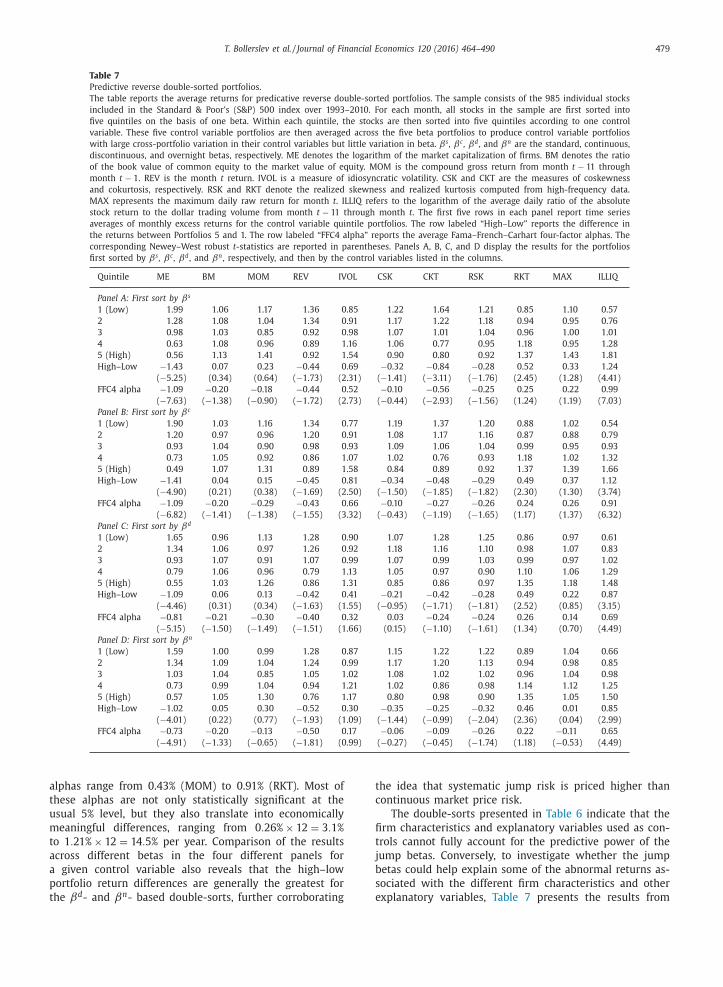
T. Bollerslev et al. / Journal of Financial Economics 120 (2016) 464–490 479
Table 7
Predictive reverse double-sorted portfolios.
The table reports the average returns for predicative reverse double-sorted portfolios. The sample consists of the 985 individual stocks
included in the Standard & Poor’s (S&P) 500 index over 1993–2010. For each month, all stocks in the sample are first sorted into
five quintiles on the basis of one beta. Within each quintile , the stocks are then sorted into five quintiles according to one control
variable. These five control variable portfolios are then averaged across the five beta portfolios to produce control variable portfolios
with large cross-portfolio variation in their control variables but little variation in beta. β s , βc , βd , and βn are the standard, continuous,
discontinuous, and overnight betas, respectively. ME denotes the logarithm of the market capitalization of firms. BM denotes the ratio
of the book value of common equity to the market value of equity. MOM is the compound gross return from month t − 11 through
month t − 1 . REV is the month t return. IVOL is a measure of idiosyncratic volatility. CSK and CKT are the measures of coskewness
and cokurtosis, respectively. RSK and RKT denote the realized skewness and realized kurtosis computed from high-frequency data.
MAX represents the maximum daily raw return for month t . ILLIQ refers to the logarithm of the average daily ratio of the absolute
stock return to the dollar trading volume from month t − 11 through month t . The first five rows in each panel report time series
averages of monthly excess returns for the control variable quintile portfolios. The row labeled “High–Low” reports the difference in
the returns between Portfolios 5 and 1. The row labeled “FFC4 alpha” reports the average Fama–French–Carhart four-factor alphas. The
corresponding Newey–West robust t -statistics are reported in parentheses. Panels A, B, C, and D display the results for the portfolios
first sorted by βs , βc , βd , and βn , respectively, and then by the control variables listed in the columns.
Quintile ME BM MOM REV IVOL CSK CKT RSK RKT MAX ILLIQ
Panel A: First sort by βs
1 (Low) 1 .99 1 .06 1 .17 1 .36 0 .85 1 .22 1 .64 1 .21 0 .85 1 .10 0 .57
2 1 .28 1 .08 1 .04 1 .34 0 .91 1 .17 1 .22 1 .18 0 .94 0 .95 0 .76
3 0 .98 1 .03 0 .85 0 .92 0 .98 1 .07 1 .01 1 .04 0 .96 1 .00 1 .01
4 0 .63 1 .08 0 .96 0 .89 1 .16 1 .06 0 .77 0 .95 1 .18 0 .95 1 .28
5 (High) 0 .56 1 .13 1 .41 0 .92 1 .54 0 .90 0 .80 0 .92 1 .37 1 .43 1 .81
High–Low −1 .43 0 .07 0 .23 −0 .44 0 .69 −0 .32 −0 .84 −0 .28 0 .52 0 .33 1 .24
(−5 .25) (0 .34) (0 .64) (−1 .73) (2 .31) (−1 .41) (−3 .11) (−1 .76) (2 .45) (1 .28) (4 .41)
FFC4 alpha −1 .09 −0 .20 −0 .18 −0 .44 0 .52 −0 .10 −0 .56 −0 .25 0 .25 0 .22 0 .99
(−7 .63) (−1 .38) (−0 .90) (−1 .72) (2 .73) (−0 .44) (−2 .93) (−1 .56) (1 .24) (1 .19) (7 .03)
Panel B: First sort by βc
1 (Low) 1 .90 1 .03 1 .16 1 .34 0 .77 1 .19 1 .37 1 .20 0 .88 1 .02 0 .54
2 1 .20 0 .97 0 .96 1 .20 0 .91 1 .08 1 .17 1 .16 0 .87 0 .88 0 .79
3 0 .93 1 .04 0 .90 0 .98 0 .93 1 .09 1 .06 1 .04 0 .99 0 .95 0 .93
4 0 .73 1 .05 0 .92 0 .86 1 .07 1 .02 0 .76 0 .93 1 .18 1 .02 1 .32
5 (High) 0 .49 1 .07 1 .31 0 .89 1 .58 0 .84 0 .89 0 .92 1 .37 1 .39 1 .66
High–Low −1 .41 0 .04 0 .15 −0 .45 0 .81 −0 .34 −0 .48 −0 .29 0 .49 0 .37 1 .12
(−4 .90) (0 .21) (0 .38) (−1 .69) (2 .50) (−1 .50) (−1 .85) (−1 .82) (2 .30) (1 .30) (3 .74)
FFC4 alpha −1 .09 −0 .20 −0 .29 −0 .43 0 .66 −0 .10 −0 .27 −0 .26 0 .24 0 .26 0 .91
(−6 .82) (−1 .41) (−1 .38) (−1 .55) (3 .32) (−0 .43) (−1 .19) (−1 .65) (1 .17) (1 .37) (6 .32)
Panel C: First sort by βd
1 (Low) 1 .65 0 .96 1 .13 1 .28 0 .90 1 .07 1 .28 1 .25 0 .86 0 .97 0 .61
2 1 .34 1 .06 0 .97 1 .26 0 .92 1 .18 1 .16 1 .10 0 .98 1 .07 0 .83
3 0 .93 1 .07 0 .91 1 .07 0 .99 1 .07 0 .99 1 .03 0 .99 0 .97 1 .02
4 0 .79 1 .06 0 .96 0 .79 1 .13 1 .05 0 .97 0 .90 1 .10 1 .06 1 .29
5 (High) 0 .55 1 .03 1 .26 0 .86 1 .31 0 .85 0 .86 0 .97 1 .35 1 .18 1 .48
High–Low −1 .09 0 .06 0 .13 −0 .42 0 .41 −0 .21 −0 .42 −0 .28 0 .49 0 .22 0 .87
(−4 .46) (0 .31) (0 .34) (−1 .63) (1 .55) (−0 .95) (−1 .71) (−1 .81) (2 .52) (0 .85) (3 .15)
FFC4 alpha −0 .81 −0 .21 −0 .30 −0 .40 0 .32 0 .03 −0 .24 −0 .24 0 .26 0 .14 0 .69
(−5 .15) (−1 .50) (−1 .49) (−1 .51) (1 .66) (0 .15) (−1 .10) (−1 .61) (1 .34) (0 .70) (4 .49)
Panel D: First sort by βn
1 (Low) 1 .59 1 .00 0 .99 1 .28 0 .87 1 .15 1 .22 1 .22 0 .89 1 .04 0 .66
2 1 .34 1 .09 1 .04 1 .24 0 .99 1 .17 1 .20 1 .13 0 .94 0 .98 0 .85
3 1 .03 1 .04 0 .85 1 .05 1 .02 1 .08 1 .02 1 .02 0 .96 1 .04 0 .98
4 0 .73 0 .99 1 .04 0 .94 1 .21 1 .02 0 .86 0 .98 1 .14 1 .12 1 .25
5 (High) 0 .57 1 .05 1 .30 0 .76 1 .17 0 .80 0 .98 0 .90 1 .35 1 .05 1 .50
High–Low −1 .02 0 .05 0 .30 −0 .52 0 .30 −0 .35 −0 .25 −0 .32 0 .46 0 .01 0 .85
(−4 .01) (0 .22) (0 .77) (−1 .93) (1 .09) (−1 .44) (−0 .99) (−2 .04) (2 .36) (0 .04) (2 .99)
FFC4 alpha −0 .73 −0 .20 −0 .13 −0 .50 0 .17 −0 .06 −0 .09 −0 .26 0 .22 −0 .11 0 .65
(−4 .91) (−1 .33) (−0 .65) (−1 .81) (0 .99) (−0 .27) (−0 .45) (−1 .74) (1 .18) (−0 .53) (4 .49)
alphas range from 0.43% (MOM) to 0.91% (RKT). Most of
these alphas are not only statistically significant at the
usual 5% level, but they also translate into economically
meaningful differences, ranging from 0 . 26% × 12 = 3 . 1%
to 1 . 21% × 12 = 14 . 5% per year. Comparison of the results
across different betas in the four different panels for
a given control variable also reveals that the high–low
portfolio return differences are generally the greatest for
the βd - and βn - based double-sorts, further corroborating
the idea that systematic jump risk is priced higher than
continuous market price risk.
The double-sorts presented in Table 6 indicate that the
firm characteristics and explanatory variables used as con-
trols cannot fully account for the predictive power of the
jump betas. Conversely, to investigate whether the jump
betas could help explain some of the abnormal returns as-
sociated with the different firm characteristics and other
explanatory variables, Table 7 presents the results from

480 T. Bollerslev et al. / Journal of Financial Economics 120 (2016) 464–490
reversing the order of the sorts, by first sorting on the
betas and then on the explanatory variables. 36 Compar-
ing the spreads in the same column across different pan-
els shows that the predictive powers of the other explana-
tory variables are generally reduced when controlling for
the jump betas, with almost all of the high–low portfolio
returns being lower (in an absolute sense) in Panels C and
D than in Panels A and B. Looking specifically at the results
in Panel A that control for the variation in the standard βs ,
the ME, IVOL, CKT, and ILLIQ sorts all yield t -statistics for
the FFC4 alphas greater than the usual critical value of two.
Meanwhile, in the double-sorts that control for the jump
betas reported in Panels C and D, only the t -statistics for
ME and ILLIQ are significant. Hence, the separate pricing
of systematic jump risk could at least in part help explain
the abnormal returns associated with idiosyncratic volatil-
ity and cokurtosis observed over the present sample. 37
6. Cross-sectional pricing regressions
The portfolio sorts discussed in Section 5 impose no
model assumptions. However, they ignore potentially im-
portant cross-sectional firm-level information by aggregat-
ing the stocks into quintile portfolios. Also, even though
the double-sorted portfolios do control for other explana-
tory variables, they control only for one variable at a time.
Hence, we turn next to a standard ( Fama and MacBeth,
1973 )- type cross-sectional approach based on firm-level
data for estimating the risk premiums associated with the
different betas, while simultaneously controlling for multi-
ple explanatory variables.
For ease of notation, let the unit time interval be
a month. The cross-sectional pricing regression for each
of the months t = 1 , 2 , . . . , T , and all of the stocks i =1 , 2 , . . . , N t available for a particular month t in the sam-
ple, could then be expressed as
r (i ) t ,t +1
= γ0 ,t + γ c β,t β
(c,i ) t + γ d
β,t β(d,i ) t + γ n
β,t β(n,i ) t
+
p ∑
j=1
γ j,t Z (i ) j,t
+ ε(i ) t ,t +1
, (14)
where r (i ) t ,t +1
denotes the excess return for stock i from
month t to month t + 1 and the explanatory variables Z (i ) j,t
and the betas β(c,i ) t , β(d,i )
t , and β(n,i ) t are measured at the
end of month t . 38 For comparison, we also estimate sim-
ilar regressions by replacing the three betas by the stan-
36 An interesting recent study, Lou, Polk, and Skouras (2015) , finds that
most of the abnormal returns on momentum strategies tend to occur
overnight, while the abnormal returns on other strategies primarily oc-
cur intraday. 37 The positive premium for IVOL observed here is counter to the id-
iosyncratic volatility puzzle first highlighted by Ang, Hodrick, Xing, and
Zhang (2006b ). However, as previously showed in the literature, the id-
iosyncratic volatility puzzle is primarily driven by small firms ( Fu, 2009 ),
firms that are dominated by retail investors ( Han and Kumar, 2013 ), and
lottery-like firms ( Bali, Cakici, and Whitelaw, 2011 ). By contrast, our sam-
ple of S&P 500 constituents consists entirely of relatively large firms. For
a recent discussion of the idiosyncratic volatility puzzle, see Stambaugh,
Yu, and Yuan (2015) . 38 Following common practice in the literature (e.g., Ang, Chen, and
Xing, 2006a , among many others), in an effort to reduce the effect of ex-
dard CAPM beta β(s,i ) t . Based on these cross-sectional re-
gression results, we then estimate the risk premiums asso-
ciated with the different betas and explanatory variables as
the time series means of the T = 204 individual monthly
gamma estimates. For k = s, c, d, n and j = 1 , . . . , p,
ˆ γ k β =
1
T
T ∑
t=1
ˆ γ k β,t , and ˆ γ j =
1
T
T ∑
t=1
ˆ γ j,t . (15)
The average risk premium estimates, with robust t -
statistics in parentheses, are reported in Table 8 for a
range of different combinations of explanatory variables.
Panel A gives the results from simple univariate regres-
sions involving a single beta measure or a single explana-
tory variable. Consistent with the standard CAPM, all the
beta risk premiums are estimated to be positive. The pre-
mium associated with βc is the highest of the four, and
that of βn is the lowest, although the t -statistic associ-
ated with βn is the highest and the t -statistic with βc
the lowest. Many of the previously showed CAPM-related
anomalies appear fairly weak in the present sample of
relatively large liquid stocks. Still, the significant positive
premiums for ILLIQ and RKT do corroborate the empiri-
cal findings in Amihud (2002) and Amaya, Christoffersen,
Jacobs, and Vasquez (2015) , respectively. The negative es-
timates for ME, CSK, and RSK are also in line with the
empirical evidence reported in Fama and French (1992) ,
Harvey and Siddique (20 0 0) , and Amaya, Christoffersen, Ja-
cobs, and Vasquez (2015) , among many others, while as
previously noted the positive albeit statistically weak pre-
mium for IVOL is counter to Ang, Hodrick, Xing, and Zhang
(2006b ).
Turning to the multiple regression results in Panel B,
Regression I shows that the standard beta βs becomes
insignificant when controlling for all the other explanatory
variables. Similarly, the risk premium for βc in Regression
II is also insignificant, suggesting that the explanatory
power of the continuous beta is effectively subsumed
by the other explanatory variables. The t -statistic for the
discontinuous beta βd in Regression III, however, is largely
unchanged from the results in the simple regression in
Panel A. For the overnight beta βn , the t -statistic for
Regression IV is even higher than in the simple regression
in Panel A.
Regressions V–XIII show the results from simulta-
neously including the continuous, discontinuous, and
overnight betas, controlling for ME, BM, MOM, and each
of the other explanatory variables in turn. The high cor-
relations across the different beta estimates, discussed
in Table 2 , invariably render lower slope coefficients
and t -statistics than in Regressions II–IV. Nonetheless,
the estimated risk premiums associated with βd and βn
remain close to significant across all the specifications
when judged by their one-sided t -statistics at the usual
5% level. The t -statistics for βc are practically zero for all
specifications, suggesting that the premium for systematic
treme observations or outliers, we winsorize the independent variables
at their 0.5% and 99.5% levels. The results from the non-winsorized re-
gressions, available upon request, are very similar to the results reported
here.

T. Bollerslev et al. / Journal of Financial Economics 120 (2016) 46 4–490 4 81
Table 8
Fama–MacBeth regressions.
The table reports the estimated regression coefficients and robust t -statistics (in parentheses) from Fama–MacBeth cross-sectional regressions for
monthly stock returns. The sample consists of the 985 individual stocks included in the Standard & Poor’s (S&P) 500 index over 1993–2010. β s , βc ,
βd , and βn are the standard, continuous, discontinuous, and overnight betas, respectively. ME denotes the logarithm of the market capitalization of
firms. BM denotes the ratio of the book value of common equity to the market value of equity. MOM is the compound gross return from month t − 11
through month t − 1 . REV is the month t return. IVOL is a measure of idiosyncratic volatility. CSK and CKT denote the measures of coskewness and
cokurtosis, respectively. RSK and RKT are the realized skewness and realized kurtosis, respectively, computed from high-frequency data. MAX represents
the maximum daily raw return for month t . ILLIQ refers to the logarithm of the average daily ratio of the absolute stock return to the dollar trading
volume from month t − 11 through month t . Panel A reports the results of simple regressions with a single explanatory variable. Panel B reports the
results of multiple regressions with more than one explanatory variable.
Panel A: Simple regressions
βs βc βd βn ME BM MOM REV IVOL CSK CKT RSK RKT MAX ILLIQ
0.86 0 .95 0 .82 0 .58 −0 .37 −0 .20 0 .01 −0 .01 0 .23 −1 .56 −0 .25 −0 .63 0 .15 0 .06 0 .31
(1.94) (1 .91) (1 .99) (2 .14) (−4 .08) (−0 .79) (0 .82) (−0 .74) (1 .36) (−1 .83) (−1 .43) (−1 .91) (1 .94) (1 .28) (3 .33)
Panel B: Multiple regressions
Regression βs βc βd βn ME BM MOM REV IVOL CSK CKT RSK RKT MAX ILLIQ
I 0 .71 −0 .45 −0 .28 0 .01 −0 .02 −0 .19 0 .77 −0 .41 −0 .18 −0 .05 0 .02 −0 .05
(1 .41) (−3 .03) (−1 .51) (1 .31) (−2 .06) (−1 .73) (1 .35) (−2 .25) (−0 .67) (−0 .92) (0 .69) (−0 .43)
II 0 .58 −0 .47 −0 .31 0 .01 −0 .02 −0 .15 0 .78 −0 .18 −0 .21 −0 .05 0 .03 −0 .03
(1 .46) (−3 .03) (−1 .66) (1 .19) (−2 .04) (−1 .36) (1 .39) (−1 .27) (−0 .78) (−1 .00) (0 .93) (−0 .22)
III 0 .55 −0 .49 −0 .33 0 .01 −0 .02 −0 .17 0 .97 −0 .15 −0 .18 −0 .04 0 .03 −0 .10
(1 .97) (−3 .10) (−1 .71) (1 .27) (−2 .07) (−1 .62) (1 .67) (−1 .06) (−0 .66) (−0 .77) (0 .80) (−0 .73)
IV 0 .43 −0 .51 −0 .32 0 .01 −0 .03 −0 .17 0 .86 −0 .13 −0 .12 −0 .03 0 .02 −0 .11
(2 .25) (−3 .09) (−1 .63) (1 .45) (−2 .16) (−1 .56) (1 .48) (−0 .90) (−0 .47) (−0 .62) (0 .50) (−0 .81)
V −0 .06 0 .29 0 .30 −0 .37 −0 .25 0 .01
(−0 .13) (1 .68) (2 .16) (−4 .45) (−0 .97) (1 .15)
V −0 .02 0 .28 0 .31 −0 .38 −0 .23 0 .00 −0 .02
(−0 .04) (1 .74) (2 .22) (−4 .59) (−1 .19) (0 .97) (−2 .17)
VII −0 .05 0 .36 0 .32 −0 .38 −0 .26 0 .01 −0 .10
(−0 .12) (1 .61) (2 .11) (−4 .96) (−1 .03) (1 .16) (−0 .99)
VIII −0 .07 0 .33 0 .29 −0 .37 −0 .28 0 .01 −0 .14
(−0 .15) (1 .72) (2 .01) (−4 .50) (−1 .12) (1 .15) (−0 .26)
IX −0 .01 0 .30 0 .28 −0 .36 −0 .28 0 .01 −0 .05
(−0 .03) (1 .76) (2 .02) (−4 .70) (−1 .14) (1 .12) (−0 .36)
X −0 .02 0 .28 0 .30 −0 .37 −0 .27 0 .01 −0 .57
(−0 .04) (1 .71) (2 .05) (−4 .49) (−1 .04) (1 .11) (−1 .94)
XI −0 .07 0 .27 0 .29 −0 .40 −0 .31 0 .01 −0 .05
(−0 .15) (1 .73) (2 .00) (−4 .69) (−1 .28) (1 .27) (−0 .85)
XII −0 .03 0 .39 0 .35 −0 .38 −0 .26 0 .01 −0 .05
(−0 .07) (1 .74) (2 .47) (−4 .86) (−1 .02) (1 .14) (−1 .68)
XIII −0 .06 0 .29 0 .28 −0 .42 −0 .24 0 .01 −0 .06
(−0 .13) (1 .76) (1 .96) (−2 .65) (−0 .92) (1 .34) (−0 .48)
XIV 0 .02 0 .31 0 .31 −0 .47 −0 .28 0 .01 −0 .02 −0 .20 0 .80 −0 .13 −0 .18 −0 .04 0 .03 −0 .08
(0 .05) (2.33) (−3 .17) (−1 .48) (1 .25) (−2 .09) (−1 .93) (1 .44) (−0 .91) (−0 .69) (−0 .80) (0 .77) (−0 .61)
XV 0 .25 0 .25 0 .25 −0 .45 −0 .28 0 .01 −0 .02 −0 .21 0 .81 −0 .17 −0 .18 −0 .02 0 .02 −0 .06
(1.96) (−2 .95) (−1 .46) (1 .33) (−2 .09) (−2 .00) (1 .41) (−1 .26) (−0 .66) (−0 .39) (0 .49) (−0 .48)
continuous market risk is fully absorbed by the premi-
ums for the two rough betas and the other explanatory
variables.
The estimated premiums for βd and βn risks are also
remarkably robust across the different specifications, with
typical values of around 0.3% for each of the rough betas.
The t -statistic for testing that the two premiums are the
same after controlling for all the other explanatory vari-
ables equals just 0.26. Hence, in Regression XIV, we re-
port the results including the three betas and all control
variables, explicitly restricting the premiums for βd and
βn risks to be the same. The estimated common rough
beta risk premium equals 0.31% with a t -statistic of 2.33. 39
39 This value is very much in line with the options-based estimate of
the aggregate equity risk premium attributable to jump tail risk of close
to 5% per year reported in Bollerslev and Todorov (2011) . That study also
Given that the cross-sectional standard deviations of βd
and βn are equal to 1.14 and 1.20, respectively, a two stan-
dard deviation change in each of the two rough betas also
translates into large and economically meaningful expected
return differences of about 2 × 1 . 14 × 0 . 33% × 12 = 9 . 03%
and 2 × 1 . 20 × 0 . 33% × 12 = 9 . 50% per year, respectively.
Regression XV further constrains all three βc , βd , and
βn risks to have the same premium. This results in a
marginally significant t -statistic of 1.96 for the beta risk
premium. However, a robust F -test easily rejects the null
suggests that the premium for jump tail risk could change over time with
changes in investors’ attitude to risk or fear. To investigate the sensitivity
of our results to the financial crisis, we have also redone the estimation
excluding January 2007 to December 2008 from the sample, resulting in a
jump beta risk premium of 0.43% and an even more significant t -statistic
of 3.07.

482 T. Bollerslev et al. / Journal of Financial Economics 120 (2016) 464–490
Fig. 3. Signature plots for betas. Panel A shows the mean value of βc (solid line) averaged across stocks and time for different sampling frequencies (labeled
in minutes on the X -axis). The dashed line gives the mean value of the mixed-frequency βc . Panel B plots the same averaged estimates for βd .
hypothesis that the three risk premiums are the same. By
contrast, the assumption that the risk premiums for βd
and βn are the same and different from the premium for
βc , as in Regression XIV, cannot be rejected.
7. Robustness checks
To further help corroborate the robustness of our find-
ings, we carry out a series of additional tests and empirical
investigations. To begin, we investigate the sensitivity of
our main empirical findings to the choice of intraday sam-
pling frequency used in the estimation of the betas, possi-
ble biases in the estimation of the betas induced by non-
synchronous trading effects, and errors-in-variables in the
cross-sectional pricing regressions stemming from estima-
tion errors in the betas. Next, we analyze how the cross-
sectional regression results and the estimated risk premi-
ums for the different betas are affected by the length of
the sample period used in the estimation of the betas and
the holding period of the future returns. Finally, we com-
pare our main results with those obtained by excluding
specific macroeconomic news announcement days in the
estimation of the betas.
7.1. Sampling frequency and beta estimation
The continuous-time framework of the empirical inves-
tigations and the consistency of the βc and βd estimates
hinge on increasingly finer sampled intraday returns. In
practice, nonsynchronous trading and other market mi-
crostructure effects invariably limit the frequency of the
data available for estimation. To assess the sensitivity of
the beta estimates to the choice of sampling frequency, we
compute betas for five different fixed sampling frequen-
cies: 5-, 25-, 75-, 125-, and 180-minute. These five sam-
pling schemes, ranging from a total of 75 observations per
day (five-minute) to only two observations per day (180-
minute), span most of the frequencies used in the liter-
ature for computing multivariate realized variation mea-
sures. The extent of market microstructure frictions varies
across different stocks. Less frequently traded stocks are
likely more prone to estimation biases in their betas from
too frequent sampling than more liquid stocks. Thus, we
also adopt a mixed-frequency strategy in which we apply
different sam pling frequencies to different stocks. We sort
all stocks into quintiles according to their ILLIQ measure
at the end of each month t . We then use the i th highest
of the five fixed sampling frequencies for stocks in the i th
illiquidity quintile ; i.e., five-minute frequency for stocks in
the lowest ILLIQ quintile (the most liquid) and 180-minute
frequency for stocks in the highest ILLIQ quintile (the least
liquid).
Fig. 3 plots the sample means averaged across time and
stocks for the resulting βc and βd estimates as a function
of the five different fixed sampling frequencies. The sample
means of the mixed-frequency beta estimates are shown as
a flat dashed line in both panels. The average βc estimates,
reported in Panel A, increase substantially from the 5- to
the 25-minute sampling frequency but appear to flatten at
around 0.93 at the 75-minute sampling frequency used in
our empirical results reported so far. The average βd es-
timates reported in Panel B, however, are remarkably sta-
ble across different sampling frequencies and close to the
average mixed-frequency value of 1.35. The specific choice
of sampling frequency within the range of values consid-
ered here appears largely irrelevant to the two discontinu-
ous beta estimates.
To further investigate the role of sampling frequency
in our key empirical findings, Table 9 reports results of
cross-sectional pricing regressions based on the different
beta estimates. Panel A gives the results obtained by vary-
ing the sampling frequency used in the estimation of βc ,
keeping the sampling frequency for the βd estimation fixed
at 75 minutes. Panel B reports the results for the differ-
ent βd estimates, using the same 75-minute βc estimates.
To conserve space, we report only results corresponding to

T. Bollerslev et al. / Journal of Financial Economics 120 (2016) 46 4–490 4 83
Table 9
Fama–MacBeth regressions with different beta estimation frequencies.
The table reports the estimated regression coefficients and robust t -statistics (in parentheses) from monthly Fama–MacBeth cross-sectional regressions
simultaneously controlling for all explanatory variables, restricting the coefficients for βd and βn to be the same. The sample consists of the 985
individual stocks included in the Standard & Poor’s (S&P) 500 index over 1993–2010. βc , βd , and βn refer to the continuous, discontinuous, and
overnight betas, respectively. ME denotes the logarithm of the market capitalization of firms. BM denotes the ratio of the book value of common equity
to the market value of equity. MOM is the compound gross return from month t − 11 through month t − 1 . REV is the month t return. IVOL is a
measure of idiosyncratic volatility. CSK and CKT denote the measures of coskewness and cokurtosis, respectively. RSK and RKT refer to the realized
skewness and realized kurtosis, respectively, computed from high-frequency data. MAX represents the maximum daily raw return for month t . ILLIQ
refers to the logarithm of the average daily ratio of the absolute stock return to the dollar trading volume from month t − 11 through month t . Panel A
reports the results for different βc estimates computed using the sampling frequencies listed in the first column labeled “Frequency.” Panel B reports
the results for different βd estimates based on the sampling frequencies in the “Frequency” column.
Frequency βc βd , βn ME BM MOM REV IVOL CSK CKT RSK RKT MAX ILLIQ
Panel A: Different βc estimates
5 minutes −0 .36 0 .34 −0 .52 −0 .30 0 .01 −2 .45 −0 .21 0 .86 −0 .06 −0 .15 −0 .04 0 .02 −0 .16
(−0 .87) (2 .57) (−3 .34) (−1 .60) (1 .37) (−2 .13) (−1 .96) (1 .54) (−0 .42) (−0 .55) (−0 .73) (0 .69) (−1 .21)
25 minutes −0 .02 0 .31 −0 .51 −0 .31 0 .01 −2 .39 −0 .21 0 .82 −0 .08 −0 .21 −0 .03 0 .03 −0 .10
(−0 .04) (2 .35) (−3 .37) (−1 .66) (1 .36) (−2 .10) (−2 .01) (1 .50) (−0 .61) (−0 .79) (−0 .69) (0 .73) (−0 .82)
75 minutes 0 .02 0 .31 −0 .47 −0 .28 0 .01 −2 .38 −0 .20 0 .80 −0 .13 −0 .18 −0 .04 0 .03 −0 .08
(0 .05) (2 .33) (−3 .17) (−1 .48) (1 .25) (−2 .09) (−1 .94) (1 .44) (−0 .91) (−0 .69) (−0 .80) (0 .77) (−0 .61)
125 minutes 0 .12 0 .27 −0 .47 −0 .30 0 .01 −2 .43 −0 .21 0 .82 −0 .15 −0 .17 −0 .03 0 .02 −0 .08
(0 .35) (2 .10) (−3 .10) (−1 .58) (1 .34) (−2 .11) (−1 .99) (1 .46) (−1 .05) (−0 .65) (−0 .59) (0 .62) (−0 .60)
180 minutes 0 .05 0 .29 −0 .48 −0 .31 0 .01 −2 .52 −0 .20 0 .88 −0 .15 −0 .17 −0 .03 0 .02 −0 .10
(0 .14) (2 .22) (−3 .17) (−1 .62) (1 .40) (−2 .20) (−1 .94) (1 .59) (−1 .11) (−0 .62) (−0 .64) (0 .68) (−0 .73)
Mix 0 .06 0 .30 −0 .42 −0 .31 0 .01 −2 .49 −0 .21 0 .86 −0 .09 −0 .18 −0 .03 0 .02 −0 .08
(0 .17) (2 .24) (−2 .87) (−1 .63) (1 .42) (−2 .18) (−1 .96) (1 .53) (−0 .66) (−0 .67) (−0 .63) (0 .61) (−0 .58)
Panel B: Different βd estimates
5 minutes 0 .12 0 .28 −0 .48 −0 .30 0 .01 −2 .39 −0 .19 0 .78 −0 .11 −0 .17 −0 .04 0 .03 −0 .08
(0 .32) (2 .10) (−3 .19) (−1 .57) (1 .28) (−2 .10) (−1 .80) (1 .40) (−0 .81) (−0 .66) (−0 .70) (0 .76) (−0 .61)
25 minutes 0 .05 0 .29 −0 .48 −0 .28 0 .01 −2 .45 −0 .20 0 .80 −0 .12 −0 .16 −0 .04 0 .03 −0 .08
(0 .15) (2 .32) (−3 .19) (−1 .47) (1 .30) (−2 .14) (−1 .88) (1 .44) (−0 .87) (−0 .59) (−0 .76) (0 .80) (−0 .61)
75 minutes 0 .02 0 .31 −0 .47 −0 .28 0 .01 −2 .38 −0 .20 0 .80 −0 .13 −0 .18 −0 .04 0 .03 −0 .08
(0 .05) (2 .33) (−3 .17) (−1 .48) (1 .25) (−2 .09) (−1 .94) (1 .44) (−0 .91) (−0 .69) (−0 .80) (0 .77) (−0 .61)
125 minutes 0 .04 0 .30 −0 .47 −0 .28 0 .01 −2 .44 −0 .21 0 .79 −0 .14 −0 .19 −0 .04 0 .03 −0 .07
(0 .10) (2 .28) (−3 .14) (−1 .51) (1 .24) (−2 .15) (−2 .02) (1 .41) (−0 .99) (−0 .71) (−0 .77) (0 .85) (−0 .58)
180 minutes 0 .04 0 .29 −0 .47 −0 .28 0 .01 −2 .47 −0 .21 0 .75 −0 .13 −0 .20 −0 .04 0 .03 −0 .07
(0 .12) (2 .22) (−3 .15) (−1 .49) (1 .25) (−2 .16) (−2 .01) (1 .35) (−0 .94) (−0 .75) (−0 .80) (0 .88) (−0 .59)
Mix 0 .08 0 .28 −0 .45 −0 .28 0 .01 −2 .44 −0 .20 0 .77 −0 .13 −0 .18 −0 .04 0 .03 −0 .07
(0 .22) (2 .20) (−3 .07) (−1 .50) (1 .26) (−2 .13) (−1 .95) (1 .37) (−0 .93) (−0 .70) (−0 .72) (0 .85) (−0 .56)
− (r (is :
1 {| r (0) s : τ |
} − (r (s
2 1 {| r (0) s : τ |
the full Regression XIV reported in Panel B of Table 8 that
restricts the premiums for the two rough betas to be the
same.
None of the t -statistics for the continuous systematic
risk premiums in Panel A is close to significant. All of the
t -statistics for the rough beta risk premiums are higher
than two. The estimated risk premiums are also very sim-
ilar across the different regressions and close to the value
of 0.31% for the benchmark Regression XIV in Table 8 . The
regressions in Panel B for the different βd estimates tell a
very similar story. The risk premiums for the rough betas
are always significant, and those for the continuous betas
are not. Overall, our key cross-sectional pricing results ap-
β(c,i ) t, − =
n
n − 1
∑ t−1 s = t−l
∑ n τ=2
[(r (i )
s : τ + r (0) s : τ−1
) 2 1 {| r (i ) s : τ + r (0)
s : τ−1 |≤k (i +0)
s,τ }4
∑ t−1 s = t−l
∑ n τ=1 (r (0)
s : τ ) 2
β(c,i ) t, + =
n
n − 1
∑ t−1 s = t−l
∑ n τ=2
[(r (i )
s : τ−1 + r (0)
s : τ ) 2 1 {| r (i ) s : τ−1
+ r (0) s : τ |≤k (i +0)
s,τ
4
∑ t−1 s = t−l
∑ n τ=1 (r (0)
s : τ )
pear robust to choice of intraday sampling frequency used
in the estimation of the βc and βd risk measures.
7.2. Nonsynchronous trading and beta estimation
The results in Section 7.1 indicate that the esti-
mated jump betas are very stable across different sam-
pling frequencies, and the continuous betas appear to be
downward-biased for the highest sampling frequencies.
This downward bias could in part be attributed to non-
synchronous trading effects. To more directly investigate
this, following the original ideas of Scholes and Williams
(1977) and Dimson (1979) , we calculate high-frequency
based lead and lag continuous betas as
) τ − r (0)
s : τ−1 ) 2 1 {| r (i )
s : τ −r (0) s : τ−1
|≤k (i −0) s,τ }
]≤k (0)
s,τ } (16)
and
i ) : τ−1
− r (0) s : τ ) 2 1 {| r (i )
s : τ−1 −r (0)
s : τ |≤k (i −0) s,τ }
]≤k (0)
s,τ } , (17)
where n denotes the number of high-frequency observa-
tions within a day used in the estimation; i.e., n = 5 for

484 T. Bollerslev et al. / Journal of Financial Economics 120 (2016) 464–490
the 75-minute sampling underlying our main empirical re-
sults. The theory behind the high-frequency betas implies
that the lead and lag betas should be asymptotically neg-
ligible and thus have no significant impact on the cross-
sectional pricing. 40
To test for this, we repeat the single-sorts in Table 4
by instead sorting the stocks according to their β(c,i ) t, − and β(c,i )
t, + estimates. The monthly return differences between
the resulting high and low quintile portfolios equal −0 . 37 %
with a t -statistic of −0 . 77 for the lagged continuous beta
sorts and 0.03% with a t -statistic of 0.17 for the lead con-
tinuous beta sorts, thus corroborating the idea that neither
the lead nor the lagged continuous betas are priced in the
cross section. Further along these lines, we also calculate
an adjusted continuous beta by adding all three continu-
ous beta estimates, β(c,i ) t, adj
≡ β(c,i ) t +
β(c,i ) t, − +
β(c,i ) t, + . Sorting by
these adjusted continuous betas produces a spread in the
returns between the high and low quintile portfolios of a
1.51%, very close to the value of 1.61% reported in Table 4 .
Taken as a whole, the results discussed in Section 7.1
together with the results for the lead–lag beta adjustments
discussed above indicate that nonsynchronous trading ef-
fects and biases in the high-frequency betas are not of
great concern. 41
7.3. Errors-in-variables in the cross-sectional pricing
regressions
Another potential concern when testing linear factor
pricing models relates to the errors-in-variables problem
arising from the first-stage estimation of the betas. As for-
mally shown by Shanken (1992) , the first-stage estimation
error generally results in an increase in the asymptotic
variance of the risk premium estimates from the second-
stage cross-sectional regressions. In our setting, however,
the betas are estimated from high-frequency data, result-
ing in lower measurement errors and, in turn, less of
an errors-in-variables problem than in traditional Fama–
MacBeth type regressions that rely on betas estimated
with lower frequency data. At the same time, this also
means that the standard adjustment procedures, as in, e.g.,
Shanken (1992) , are not applicable in the present con-
text. 42
40 It is not possible to similarly adjust the jump betas by including leads
and lags in their calculation. The lead–lag adjustment for the continuous
betas relies on the notion that the true high-frequency returns are ap-
proximately serially uncorrelated. However, the construction of the jump
betas is based on higher order powers of the high-frequency returns, and
the squared returns, in particular, are clearly not serially uncorrelated.
Meanwhile, the signature plots for the jump betas in Panel B of Fig. 3
show that the estimates of the jump betas are very robust to the choice
of sampling frequency and, as such, much less prone to any systematic
biases arising from nonsynchronous trading effects. 41 We also experimented with the use of alternative discontinuous beta
estimates based on simple OLS regressions for the high-frequency returns
that exceed a jump threshold. The results from the corresponding port-
folio sorts and Fama–MacBeth regressions were generally close to the re-
sults based on the discontinuous beta estimator in Eq. (13) formally de-
veloped in Todorov and Bollerslev (2010) that we rely on throughout the
paper. 42 Formally accounting for the estimation errors in the high-frequency
betas would require a new asymptotic framework in which both the time
Instead, we conduct a small-scale Monte Carlo ex-
periment by appropriately perturbing the high-frequency
beta estimates. For β(c,i ) t and
β(d,i ) t , we rely on the re-
sults in Todorov and Bollerslev (2010) to generate repli-
cates { β(c,i, rep ) t } and { β(d,i, rep )
t } from two independent nor-
mal distributions with means equal to the estimated
β(c,i ) t
and
β(d,i ) t , respectively, and standard deviations equal to
the corresponding theoretical asymptotic standard errors.
For β(n,i ) t , we rely on a bootstrap procedure to gener-
ate random samples of β(n,i, rep ) t from the actual sam-
pling distribution. Given a random sample of the three
betas ( β(c,i, rep ) t , β(d,i, rep )
t , and
β(n,i, rep ) t ) , we then estimate
the key Fama–MacBeth Regression XIV in Table 8 based
on the perturbed beta estimates keeping all of the other
controls the same. We repeat the simulations a total of
100 times.
The resulting simulation-based estimates for the risk
premiums are in the range of -0.12 to 0.27 for βc with t -
statistic between -0.24 and 0.87 and in the range of 0.20
to 0.38 with t -statistic between 1.62 and 3.16 for βd and
βn . The magnitudes of these simulated risk premiums and
their t -statistics are all fairly close to the values for the ac-
tual regression reported in Table 8 , thus confirming that
the errors-in-variables problem is not of major concern
in the present context and that it does not materially af-
fect the statistical or economic significance of the rough
betas.
7.4. Beta estimation and return holding periods
All the cross-sectional pricing regressions in Tables 8
and 9 are based on betas estimated from returns over
the past year and a future one-month return holding pe-
riod. These are typical estimation and holding periods
used to test for the significant pricing ability of explana-
tory variables and risk factors. To assess the robustness
of our results to different lagged beta estimation peri-
ods ( L ) and longer future return horizons ( H ), Table 10
reports results based on shorter three- and six-month
beta estimates and longer 3-, 6- and 12-month prediction
horizons. 43
Regressions I–V pertain to the standard beta. Although
the regression coefficients associated with the standard
beta seem to increase with the forecast horizon, their t -
statistics are at most weakly significant. Regressions VI–X
pertain to the continuous and rough betas. The regressions
show that the t -statistics associated with the two rough
betas are always significant and that the continuous sys-
tematic risk is not priced in the cross section. In fact, if
anything, the results for the shorter estimation periods and
longer return horizons are even more significant than the
results for the baseline Regression XIV in Panel B of Table 8
and the typical choice of L = 12 and H = 1.
span of the data used for the cross-sectional regression-based estimates
of the risk premiums and the sampling frequency used for the estimation
of the betas go to infinity. We leave this for future work. 43 All of the cross-sectional regressions are estimated monthly. The ro-
bust t -statistics for the longer H = 3-, 6- and 12-month return horizons
explicitly adjust for the resulting overlap in the return observations.

T. Bollerslev et al. / Journal of Financial Economics 120 (2016) 46 4–490 4 85
Table 10
Fama–MacBeth regressions with different beta estimation periods and return holding horizons.
The table reports the estimated regression coefficients and robust t -statistics (in parentheses) from Fama–MacBeth cross-sectional regressions for pre-
dicting the next H -month cumulative returns. The sample consists of the 985 individual stocks included in the Standard & Poor’s (S&P) 500 index over
1993–2010. The regressions simultaneously control for all explanatory variables, restricting the coefficients for βd and βn to be the same. The betas
are computed from the previous L -month high-frequency returns. β s , βc , βd , and βn refer to the standard, continuous, discontinuous, and overnight
betas, respectively. ME denotes the logarithm of the market capitalization of firms. BM denotes the ratio of the book value of common equity to the
market value of equity. MOM is the compound gross return from month t − 11 through month t − 1 . REV is the month t return. IVOL is a measure
of idiosyncratic volatility. CSK and CKT denote the measures of coskewness and cokurtosis, respectively. RSK and RKT refer to the realized skewness
and realized kurtosis, respectively, computed from high-frequency data. MAX represents the maximum daily raw return for month t . ILLIQ refers to the
logarithm of the average daily ratio of the absolute stock return to the dollar trading volume from month t − 11 through month t .
Regression L H βs βc βd , βn ME BM MOM REV IVOL CSK CKT RSK RKT MAX ILLIQ
I 3 1 0 .45 −0 .41 −0 .34 0 .00 −0 .03 −0 .09 0 .88 −0 .45 −0 .18 −0 .14 0 .05 0 .09
(1 .63) (−2 .32) (−1 .66) (0 .99) (−2 .75) (−0 .69) (1 .40) (−3 .04) (−0 .63) (−2 .24) (1 .44) (0 .59)
II 6 1 0 .67 −0 .38 −0 .34 0 .00 −0 .03 −0 .14 0 .87 −0 .53 −0 .18 −0 .12 0 .06 0 .10
(1 .64) (−2 .28) (−1 .71) (0 .96) (−2 .81) (−1 .17) (1 .37) (−3 .27) (−0 .63) (−2 .01) (1 .55) (0 .70)
III 12 3 2 .05 −0 .70 −0 .73 0 .02 −0 .05 −0 .16 2 .04 −1 .57 −0 .37 −0 .36 0 .13 0 .66
(1 .63) (−1 .45) (−1 .64) (1 .37) (−1 .86) (−0 .70) (1 .46) (−3 .11) (−0 .67) (−2 .77) (1 .82) (1 .38)
IV 12 6 4 .25 −1 .59 −1 .53 0 .03 0 .00 0 .36 3 .28 −2 .42 −0 .96 −0 .49 0 .03 1 .21
(1 .48) (−1 .39) (−1 .74) (1 .09) (−0 .06) (0 .87) (1 .32) (−2 .43) (−0 .89) (−1 .45) (0 .29) (1 .05)
V 12 12 9 .57 −5 .55 −3 .76 0 .05 0 .09 0 .72 3 .73 −3 .34 −1 .35 −0 .59 0 .07 0 .24
(1 .42) (−1 .95) (−1 .73) (1 .02) (0 .96) (1 .23) (0 .79) (−1 .77) (−0 .73) (−0 .67) (0 .36) (0 .10)
VI 3 1 −0 .30 0 .43 −0 .41 −0 .34 0 .00 −0 .03 −0 .19 0 .76 −0 .23 −0 .14 −0 .14 0 .05 0 .07
(−1 .10) (3 .48) (−2 .58) (−1 .69) (0 .94) (−2 .78) (−1 .68) (1 .24) (−1 .66) (−0 .48) (−2 .53) (1 .49) (0 .53)
VII 6 1 −0 .45 0 .55 −0 .42 −0 .34 0 .00 −0 .03 −0 .21 0 .85 −0 .22 −0 .16 −0 .12 0 .06 0 .05
(−1 .32) (4 .15) (−2 .63) (−1 .70) (0 .90) (−2 .87) (−1 .91) (1 .37) (−1 .61) (−0 .56) (−2 .26) (1 .70) (0 .39)
VIII 12 3 −1 .66 1 .65 −0 .84 −0 .72 0 .01 −0 .05 −0 .32 2 .50 −0 .65 −0 .39 −0 .34 0 .14 0 .46
(−1 .39) (3 .94) (−1 .86) (−1 .60) (1 .27) (−1 .97) (−1 .52) (1 .86) (−2 .12) (−0 .74) (−2 .85) (1 .92) (1 .11)
IX 12 6 −1 .35 2 .73 −1 .73 −1 .40 0 .03 −0 .01 0 .02 4 .01 −1 .05 −1 .02 −0 .39 0 .05 0 .96
(−0 .50) (3 .45) (−1 .67) (−1 .59) (1 .06) (−0 .23) (0 .06) (1 .64) (−1 .65) (−1 .00) (−1 .40) (0 .50) (0 .99)
X 12 12 3 .82 4 .07 −5 .42 −3 .15 0 .05 0 .08 −0 .08 4 .85 −1 .65 −1 .33 −0 .18 0 .08 0 .35
(0 .65) (3 .28) (−2 .04) (−1 .59) (1 .00) (0 .89) (−0 .11) (1 .01) (−1 .09) (−0 .72) (−0 .23) (0 .39) (0 .17)
44 Patton and Verardo (2012) also show that standard realized betas cal-
culated from high-frequency intraday data tend to be higher on individual
firms’ earnings announcement days. 45 Andersen, Bollerslev, Diebold, and Vega (2003) provide a comprehen-
sive list of US macroeconomic news announcements and their release
times. 46 Lucca and Moench (2015) have also recently shown large average
pre-FOMC one-day equity returns in anticipation of monetary policy
decisions.
The significance of the results for the longer 3-, 6-,
and 12-month return horizons also highlights nontrivial
persistence in the cross-sectional predictability. Converting
the resulting estimates for the different return horizons
to an annual level implies rough beta risk premiums of
1 . 65% × 4 = 6 . 60% , 2 . 73% × 2 = 5 . 46% , and 4 . 07 × 1 = 4 . 07%
per year, respectively, compared with 0 . 31 × 12 = 3 . 72%
per year for the one-month future return horizon implied
by Regression XIV in Table 8 .
While ME, REV, and RKT are each significant in one or
more of the regressions reported in Table 10 , they are not
systematically so. Short-term reversal and realized kurto-
sis, in particular, both lose their significance for the longer
6- and 12-month holding periods. The only variable that
remains highly significant across all different estimation
periods and return predictability horizons is the rough beta
risk premium.
7.5. Betas and macroeconomic news announcements
An extensive literature has been devoted to studying
the effects of macroeconomic news announcements on as-
set prices. Andersen, Bollerslev, and Diebold (2007a ), Lee
(2012) , and Lahaye, Laurent, and Neely (2011) have all
sought to relate jumps in high-frequency asset prices, with
the significant jumps identified through similar techniques
to the ones used here, to regularly scheduled macroe-
conomic news releases. Related to this, Savor and Wil-
son (2014) have also recently argued that cross-sectional
return patterns are different on news announcement
days. 44
To investigate whether macroeconomic announcement
days confound our beta estimates and the significant cross-
sectional relation between the two rough betas and ex-
pected stock returns, we exclude three specific announce-
ment days in our estimation of βc , βd , and βn , including
days when the employment report (Employment) and the
US Producer Price Index (PPI) are announced by the Bureau
of Labor Statistics and days when scheduled interest rates
are announced by the Federal Open Market Committee
(FOMC). Employment and PPI are both announced monthly
at 8:30 a.m. before the stock market officially opens, and
FOMC is announced at 2:15 p.m. every six weeks. 45
Relying on the same test for significant intraday jumps
used above, Fig. 4 compares the average jump intensity for
the S&P 500 market portfolio for the three announcement
days and all other days in the sample (Non-Ann), as a func-
tion of the time of day. Not surprisingly, the FOMC an-
nouncements at 2:15 p.m. have the greatest intraday effect,
increasing the jump intensity from an average of about 1%
per day on non-announcement days to 9% on FOMC days. 46

486 T. Bollerslev et al. / Journal of Financial Economics 120 (2016) 464–490
Fig. 4. Jump intensity and macro announcement. The figure plots the average estimated jump intensity (probability) for the Standard & Poor’s (S&P)
500 market portfolio across regular trading hours on Federal Open Market Committee (FOMC) announcement days, employment report (Employment)
announcement days, US Producer Price Index (PPI) announcement days, and all other days (Non-Ann).
Table 11
Fama–MacBeth regressions excluding macroeconomic news announcement days.
The table reports the estimated regression coefficients and robust t -statistics (in parentheses) from monthly Fama–MacBeth cross-sectional regressions
simultaneously controlling for all explanatory variables, restricting the coefficients for βd and βn to be the same. The sample consists of the 985
individual stocks included in the Standard & Poor’s (S&P500) index over 1993–2010. The betas are calculated excluding Federal Open Market Committee
(FOMC), employment report (Employment), and US Producer Price Index (PPI) announcement days in the estimation. βc , βd , and βn refer to the
continuous, discontinuous, and overnight betas, respectively. ME denotes the logarithm of the market capitalization of firms. BM denotes the ratio of
the book value of common equity to the market value of equity. MOM is the compound gross return from month t − 11 through month t − 1 . REV is
the month t return. IVOL is a measure of idiosyncratic volatility. CSK and CKT denote the measures of coskewness and cokurtosis, respectively. RSK and
RKT refer to the realized skewness and realized kurtosis, respectively, computed from high-frequency data. MAX represents the maximum daily raw
return for month t . ILLIQ refers to the logarithm of the average daily ratio of the absolute stock return to the dollar trading volume from month t − 11
through month t .
Regression βc βd , βn ME BM MOM REV IVOL CSK CKT RSK RKT MAX ILLIQ
I −0 .11 0 .30 −0 .37 −0 .25 0 .01
(−0 .25) (2 .32) (−4 .40) (−0 .93) (1 .03)
II −0 .09 0 .30 −0 .38 −0 .23 0 .00 −0 .02
(−0 .21) (2 .28) (−4 .51) (−1 .13) (0 .84) (−2 .12)
III −0 .07 0 .33 −0 .39 −0 .26 0 .00 −0 .09
(−0 .15) (2 .31) (−5 .04) (−1 .00) (1 .04) (−0 .92)
IV −0 .09 0 .30 −0 .38 −0 .28 0 .00 −0 .23
(−0 .21) (2 .26) (−4 .51) (−1 .09) (1 .02) (−0 .43)
V −0 .04 0 .29 −0 .37 −0 .29 0 .00 −0 .04
(−0 .10) (2 .30) (−4 .72) (−1 .12) (0 .99) (−0 .31)
VI −0 .08 0 .29 −0 .37 −0 .26 0 .00 −0 .59
(−0 .18) (2 .30) (−4 .43) (−0 .98) (0 .99) (−2 .01)
VII −0 .11 0 .28 −0 .41 −0 .31 0 .01 −0 .06
(−0 .25) (2 .27) (−4 .63) (−1 .24) (1 .16) (−0 .89)
VIII −0 .05 0 .36 −0 .39 −0 .26 0 .00 −0 .05
(−0 .12) (2 .56) (−4 .87) (−1 .00) (1 .02) (−1 .61)
IX −0 .11 0 .28 −0 .44 −0 .23 0 .01 −0 .08
(−0 .26) (2 .29) (−2 .74) (−0 .87) (1 .21) (−0 .60)
X −0 .01 0 .31 −0 .50 −0 .29 0 .00 −0 .02 −0 .22 0 .81 −0 .12 −0 .17 −0 .05 0 .03 −0 .10
(−0 .04) (2 .33) (−3 .33) (−1 .54) (1 .14) (−2 .16) (−2 .05) (1 .46) (−0 .84) (−0 .63) (−0 .89) (0 .95) (−0 .77)
XI 0.24 −0 .47 −0 .28 0 .01 −0 .02 −0 .22 0 .81 −0 .17 −0 .17 −0 .02 0 .02 −0 .08
(1.95) (−3 .05) (−1 .49) (1 .27) (−2 .13) (−2 .08) (1 .41) (−1 .23) (−0 .61) (−0 .45) (0 .66) (−0 .62)
The employment report also makes a market jump more
likely in the first few minutes of trading, although not dra-
matically so. Employment and PPI are both announced be-
fore the market officially opens and, thus, can be expected
to affect estimation of the overnight betas the most.
Table 11 reports results of the full firm-level cross-
sectional regressions excluding the three different types of
announcement days. Both the size and the statistical sig-
nificance of the risk premium estimates are very similar
to those in Table 8 , Panel B. In fact, the estimated risk pre-
mium for the discontinuous and overnight betas in Regres-
sion X in Table 11 is identical within two decimal points to
the estimate from Regression XIV in Table 8 . The predictive
power and significant cross-sectional pricing ability of the

T. Bollerslev et al. / Journal of Financial Economics 120 (2016) 46 4–490 4 87
two rough betas do not appear to be solely driven by im-
portant macroeconomic news announcements.
8. Conclusions
Building on a general continuous-time representation
for the return on the aggregate market portfolio cou-
pled with an economy-wide pricing kernel that separately
prices market diffusive and jump risks, we show how stan-
dard asset pricing theory naturally results in separate risk
premiums for continuous, or smooth, market betas and
discontinuous, or rough, market betas. Importantly, our
theoretical framework explicitly allows for other system-
atic risk factors to enter the pricing kernel and possibly
affect the cross-sectional pricing. Only if nonmarket risks
are not priced, and the premiums for continuous and jump
market risks are the same, does the standard conditional
CAPM hold.
Motivated by these theoretical results, we empirically
investigate whether market diffusive and jump risks are
priced differently in the cross section of expected stock re-
turns. Our empirical investigations rely on a novel high-
frequency data set for a large cross section of individual
stocks together with new econometric techniques for sepa-
rately estimating continuous, discontinuous, and overnight
betas. We find that the discontinuous and overnight be-
tas are different from, and more cross-sectionally dispersed
than, the continuous and standard CAPM betas. When we
sort individual stocks by the different betas, we find that
stocks with high discontinuous and overnight betas earn
significantly higher returns than stocks with low discon-
tinuous and overnight betas, while at best only a weak re-
lation exists between a stock’s return and its continuous
beta. We also find that the estimated risk premiums for
the discontinuous and overnight betas to be both statis-
tically significant and indistinguishable from one another
and that this rough beta risk cannot be explained by a long
list of other firm characteristics and explanatory variables
commonly employed in the literature. In contrast, the esti-
mated continuous beta risk premium is insignificant.
Intuitively, market jumps more likely reflect true infor-
mation surprises than do continuous price moves, which
could simply be attributed to random noise in the price
formation process. Moreover, important news is often an-
nounced during overnight non-trading hours. 47 As such,
the two rough betas could more accurately reflect the sys-
tematic market price risks that are priced than do the con-
tinuous betas and the standard conditional CAPM betas
that do not differentiate between smooth and rough mar-
ket price moves.
The theoretical setup in Section 2 that motivates our
empirical investigations is deliberately very general. How-
ever, a more formal investigation into the reasons behind
the differences in the pricing of the smooth and rough be-
tas and whether the differences could be explained by dif-
47 Conversely, Berkman, Koch, Tuttle, and Zhang (2012) and Lou, Polk,
and Skouras (2015) find that institutional investors tend to trade rela-
tively more during the day and individual investors trade relatively more
overnight, thus indirectly suggesting that the overnight betas could be
more susceptible to the influence of noise trading.
ferent loadings on diffusive and jump fundamental shocks
or differences of opinion and learning, possibly influenced
by behavioral effects, would be very interesting. We leave
this for future research.
Appendix A
A.1. High-frequency data cleaning
We begin by removing entries that satisfy at least one
of the following criteria: a time stamp outside the ex-
change open window between 9:30 a.m. and 4:00 p.m.; a
price less than or equal to zero; a trade size less than or
equal to zero; corrected trades, i.e., trades with Correction
Indicator, CORR, other than 0, 1, or 2; and an abnormal sale
condition, i.e., trades for which the Sale Condition, COND,
has a letter code other than @, ∗, E, F, @E, @F, ∗E and
∗F. We
then assign a single value to each variable for each sec-
ond within the 9:30 a.m.–4:00 p.m. time interval. If one
or multiple transactions have occurred in that second, we
calculate the sum of volumes, the sum of trades, and the
volume-weighted average price within that second. If no
transaction has occurred in that second, we enter zero for
volume and trades. For the volume-weighted average price,
we use the entry from the nearest previous second, i.e.,
forward-filtering. If no transaction has occurred before that
second, we use the entry from the nearest subsequent sec-
ond, i.e., backward-filtering. Motivated by our analysis of
the trading volume distribution across different exchanges
over time, we purposely incorporate information from all
exchanges covered by the TAQ database. 48
A.2. Additional explanatory variables
Our empirical investigations rely on the following ex-
planatory variables and firm characteristics.
• Size (ME): Following Fama and French (1993) , a firm’s
size is measured at the end of June by its market
value of equity—the product of the closing price and
the number of shares outstanding (in millions of dol-
lars). Market equity is updated annually and is used to
explain returns over the subsequent 12 months. Follow-
ing common practice, we also transform the size vari-
able by its natural logarithm to reduce skewness.
• Book-to-market ratio (BM): Following Fama and French
(1992) , the book-to-market ratio in June of year t is
computed as the ratio of the book value of common
equity in fiscal year t − 1 to the market value of eq-
uity (size) in December of year t − 1 . 49 BM for fiscal
year t is used to explain returns from July of year t + 1
through June of year t + 2 . The time gap between BM
and returns ensures that information on BM is publicly
available prior to the returns.
• Momentum (MOM): Following Jegadeesh and Titman
(1993) , the momentum variable at the end of month t
48 Further details on the exchange analysis are available upon request. 49 Book common equity is defined as book value of stockholders’ equity,
plus balance sheet deferred taxes and investment tax credit (if available),
minus book value of preferred stock for fiscal year t − 1 .

488 T. Bollerslev et al. / Journal of Financial Economics 120 (2016) 464–490
is defined as the compound gross return from month
t − 11 through month t − 1 ; i.e., skipping the short-
term reversal month t . 50
• Reversal (REV): Following Jegadeesh (1990) and
Lehmann (1990) , the short-term reversal variable
at the end of month t is defined as the return over that
same month t .
• Idiosyncratic volatility (IVOL): Following Ang, Hodrick,
Xing, and Zhang (2006b ), a firm’s idiosyncratic volatil-
ity at the end of month t is computed as the standard
deviation of the residuals from the regression based on
the daily return regression:
r i,d − r f,d = αi + βi (r 0 ,d − r f,d ) + γi SMB d
+ φi HML d + εi,d , (18)
where r i, d and r 0, d are the daily returns of stock i and
the market portfolio on day d , respectively, and SMB d
and HML d denote the daily Fama and French (1993) size
and book-to-market factors.
• Coskewness (CSK): Following Harvey and Siddique
(20 0 0) and Ang, Chen, and Xing (2006a ), the coskew-
ness of stock i at the end of month t is estimated using
daily returns for month t as
CSK i,t =
1 N
∑
d (r i,d − r i )(r 0 ,d − r 0 ) 2 √
1 N
∑
d (r i,d − r i ) 2 ( 1 N
∑
d (r 0 ,d − r 0 ) 2 ) , (19)
where N denotes the number of trading days in month
t, r i, d and r 0, d are the daily returns of stock i and the
market portfolio on day d , respectively, and r i and r 0 denote the corresponding average daily returns.
• Cokurtosis (CKT): Following Ang, Chen, and Xing
(2006a ), the cokurtosis of stock i at the end of month t
is estimated using the daily returns for month t as
CKT i,t =
1 N
∑
d (r i,d − r i )(r 0 ,d − r 0 ) 3 √
1 N
∑
d (r i,d − r i ) 2 ( 1 N
∑
d (r 0 ,d − r 0 ) 2 ) 3 / 2 , (20)
where variables are the same as for CSK.
• Realized skewness (RSK): Following Amaya, Christof-
fersen, Jacobs, and Vasquez (2015) , the realized skew-
ness for stock i on day d is constructed from high-
frequency data as
RSK i,d =
√
L ∑ L
l=1 r 3 i,d,l
( ∑ L
l=1 r 2 i,d,l
) 3 / 2 , (21)
where r i, d, l r efers t o the l th intraday return on day d
for stock i and L denotes the number of intraday returns
available on day d . Consistent with Amaya, Christof-
fersen, Jacobs, and Vasquez (2015) , we use five-minute
returns from 9:45 a.m. to 4:00 p.m. so that for the full
intraday time period L = 75 . The RSK for stock i at the
end of month t is computed as the average of the daily
RSK i,d for that month.
• Realized kurtosis (RKT): Following Amaya, Christof-
fersen, Jacobs, and Vasquez (2015) , the realized kurtosis
50 Jegadeesh (1990) shows that monthly returns on many individual
stocks are significantly and negatively serially correlated.
for stock i on day d is computed as
RKT i,d =
L ∑ L
l=1 r 4 i,d,l
( ∑ L
l=1 r 2 i,d,l
) 2 , (22)
where variables and estimation details are the same as
for RSK.
• Maximum daily return (MAX): Following Bali, Cakici,
and Whitelaw (2011) , the MAX variable for stock i and
month t is defined as the largest total daily return ob-
served over that month.
• Illiquidity (ILLIQ): Following Amihud (2002) , the illiq-
uidity for stock i at the end of month t is measured as
the average daily ratio of the absolute stock return to
the dollar trading volume from month t − 11 through
month t :
ILLIQ i,t =
1
N
∑
d
( | r i,d | volume i,d × price i,d
), (23)
where volume i, d is the daily trading volume, price i, d is
the daily price, and other variables are as defined be-
fore. We further transform the illiquidity measure by its
natural logarithm to reduce skewness.
References
Aït-Sahalia, Y. , 2004. Disentangling volatility from jumps. Journal of Fi-
nancial Economics 74, 487–528 . Alexeev, V., Dungey, M., Yao, W., 2015. Time-varying continuous and jump
betas: the role of firm characteristics and periods of stress. Unpub- lished working paper. University of Tasmania and Cambridge Univer-
sity, Tasmania, Australia, and Cambridge, UK. Amaya, D. , Christoffersen, P. , Jacobs, K. , Vasquez, A. , 2015. Does realized
skewness predict the cross section of equity returns? Journal of Fi- nancial Economics 118, 135–167 .
Amihud, Y. , 2002. Illiquidity and stock returns: cross section and time se-
ries effects. Journal of Financial Markets 5, 31–56 . Andersen, T.G. , Bollerslev, T. , Diebold, F.X. , 2007a. Roughing it up: dis-
entangling continuous and jump components in measuring, model- ing, and forecasting asset return volatility. Review of Economics and
Statistics 89, 701–720 . Andersen, T.G. , Bollerslev, T. , Diebold, F.X. , Labys, P. , 2001. The distribution
of realized exchange rate volatility. Journal of the American Statistical
Association 42, 42–55 . Andersen, T.G. , Bollerslev, T. , Diebold, F.X. , Vega, C. , 2003. Micro effects of
macro annoucements: real-time price discovery in foreign exchange. American Economic Review 93, 38–62 .
Andersen, T.G. , Bollerslev, T. , Diebold, F.X. , Vega, C. , 2007b. Real-time pricediscovery in stock, bond, and foreign exchange markets. Journal of In-
ternational Economics 73, 251–277 .
Andersen, T.G. , Bollerslev, T. , Diebold, F.X. , Wu, G. , 2005. A framework forexploring the macroeconomic determinants of systematic risk. Amer-
ican Economic Review 95, 398–404 . Andersen, T.G. , Bollerslev, T. , Diebold, F.X. , Wu, G. , 2006. Realized beta:
persistence and predictability. In: Fomby, T., Terrell, D. (Eds.), In: Ad- vances in Econometrics: Econometric Analysis of Economic and Finan-
cial Time Series, Vol. 20, Part 2. Emerald Group Publishing Limited,
Bingley, UK, pp. 1–39 . Andersen, T.G. , Bollerslev, T. , Huang, X. , 2011. A reduced form framework
for modeling volatility of speculative prices based on realized varia- tion measures. Journal of Econometrics 160, 176–189 .
Ang, A. , Chen, J. , 2002. Asymmetric correlations of equity portfolios. Jour- nal of Financial Economics 63, 443–494 .
Ang, A. , Chen, J. , Xing, Y. , 2006a. Downside risk. Review of Financial Stud-
ies 19, 1191–1239 . Ang, A. , Hodrick, R. , Xing, Y. , Zhang, X. , 2006b. The cross section of volatil-
ity and expected returns. Journal of Finance 61, 259–299 . Bali, T.G. , Cakici, N. , Whitelaw, R. , 2011. Maxing out: stocks as lotteries and
the cross section of expected returns. Journal of Financial Economics 99, 427–446 .

T. Bollerslev et al. / Journal of Financial Economics 120 (2016) 46 4–490 4 89
Bali, T. G., Engle, R. F., Tang, Y., 2015. Dynamic conditional beta is alive andwell in the cross section of daily stock returns. Unpublished working
paper. Georgetown University, New York University, and Fordham Uni-versity, Washington, DC, and New York, NY.
Bansal, R. , Yaron, A. , 2004. Risks for the long run: a potential resolutionof asset pricing puzzles. Journal of Finance 59, 1481–1509 .
Banz, R.W. , 1981. The relationship between return and market value of
common stock. Journal of Financial Economics 9, 3–18 . Barndorff-Nielsen, O.E. , Hansen, P.R. , Lunde, A. , Shephard, N. , 2009. Real-
ized kernels in practice: trades and quotes. Econometrics Journal 12,C1–C32 .
Barndorff-Nielsen, O.E. , Shephard, N. , 2003. Realized power variation andstochastic volatility models. Bernoulli 9, 243–265 .
Barndorff-Nielsen, O.E. , Shephard, N. , 2004a. Econometric analysis of re-alized covariation: high-frequency-based covariance, regression, and
correlation in financial economics. Econometrica 72, 885–925 .
Barndorff-Nielsen, O.E. , Shephard, N. , 2004b. Power and bipower variationwith stochastic volatility and jumps. Journal of Financial Econometrics
2, 1–37 . Barndorff-Nielsen, O.E. , Shephard, N. , 2006. Econometrics of testing for
jumps in financial economics using bipower variation. Journal of Fi-nancial Econometrics 4, 1–30 .
Barndorff-Nielsen, O.E. , Shephard, N. , 2007. Variation, jumps, market fric-
tions and high frequency data in financial econometrics. In: Blun-dell, R., Torsten, P., Newey, W.K (Eds.), Advances in Economics and
Econometrics: Theory and Applications. Econometric Society mono-graphs. Cambridge University Press, Cambridge, UK, pp. 328–372 .
Basu, S. , 1977. Investment performance of common stocks in relation totheir price-earnings ratios: a test of the efficient market hypothesis.
Journal of Finance 32, 663–682 .
Basu, S. , 1983. The relationship between earnings yield, market value, andreturn for NYSE common stocks: further evidence. Journal of Financial
Economics 12, 129–156 . Berkman, H. , Koch, P. , Tuttle, L. , Zhang, Y. , 2012. Paying attention:
overnight returns and the hidden cost of buying at the open. Journalof Financial and Quantitative Analysis 47, 715–741 .
Bhandari, L.C. , 1988. Debt/equity ratio and expected common stock re-
turns: empirical evidence. Journal of Finance 43, 507–528 . Blume, M. , 1970. Portfolio theory: a step toward its practical application.
Journal of Business 43, 152–173 . Bollerslev, T. , Engle, R. , Wooldridge, J. , 1988. A capital asset pricing model
with time-varying covariances. Journal of Political Economy 96, 116–131 .
Bollerslev, T. , Law, T.H. , Tauchen, G. , 2008. Risk, jumps, and diversification.
Journal of Econometrics 144, 234–256 . Bollerslev, T. , Sizova, N. , Tauchen, G. , 2012. Volatility in equilibrium: asym-
metries and dynamic dependencies. Review of Finance 16, 31–80 . Bollerslev, T. , Todorov, V. , 2011. Tails, fears, and risk premia. Journal of Fi-
nance 66, 2165–2221 . Bollerslev, T. , Todorov, V. , Li, S.Z. , 2013. Jump tails, extreme dependencies,
and the distribution of stock returns. Journal of Econometrics 172,
307–324 . Bollerslev, T. , Zhang, B.Y. , 2003. Measuring and modeling systematic risk
in factor pricing models using high-frequency data. Journal of Empir-ical Finance 10, 533–558 .
Branch, B. , Ma, A. , 2012. The overnight return: the invisible hand behindthe intraday return. Journal of Applied Finance 22 (2), 90–100 .
Campbell, J. , Cochrane, J. , 1999. By force of habit: a consumption-basedexplanation of aggregate stock market behavior. Journal of Political
Economy 107, 205–251 .
Cliff, M., Cooper, M., Gulen, H., 2008. Return differences between tradingand non-trading hours: like night and day. Unpublished working pa-
per. University of Utah, Analysis Group, and Purdue University, SaltLake City, UT, Boston, MA, and West Lafayette, IN.
Corradi, V., Distaso, W., Fernandes, M., 2013. Conditional alphas and real-ized betas. Unpublished working paper. University of Warwick, Impe-
rial College London, and Queen Mary University of London, Coventry,
UK, and London, UK. Cremers, M. , Halling, M. , Weinbaum, D. , 2015. Aggregate jump and volatil-
ity risk in the cross section of stock returns. Journal of Finance 70,577–614 .
Dimson, E. , 1979. Risk measurement when shares are subject to infre-quent trading. Journal of Financial Economics 7, 197–226 .
Duffie, D. , Pan, J. , Singleton, K. , 20 0 0. Transform analysis and asset pricing
for affine jump-diffusions. Econometrica 68, 1343–1376 . Eraker, B. , Johannes, M. , Polson, N. , 2003. The impact of jumps in volatility
and returns. Journal of Finance 58, 1269–1300 . Fama, E.F. , Fisher, L. , Jensen, M. , Roll, R. , 1969. The adjustment of stock
prices to new information. International Economic Review 10, 1–21 .
Fama, E.F. , French, K.R. , 1992. The cross section of expected stock returns.Journal of Finance 47, 427–465 .
Fama, E.F. , French, K.R. , 1993. Common risk factors in the returns onstocks and bonds. Journal of Financial Economics 33, 3–56 .
Fama, E.F. , French, K.R. , 2006. The value premium and the CAPM. Journalof Finance 61, 2163–2185 .
Fama, E.F. , MacBeth, J.D. , 1973. Risk, return, and equilibrium: empirical
tests. Journal of Political Economy 81 (3), 607–636 . Ferson, W. , Kandel, S. , Stambaugh, R.F. , 1987. Tests of asset pricing with
time-varying expected risk premiums and market betas. Journal of Fi-nance 42, 201–220 .
Fleming, M.J. , Remolona, E.M. , 1999. Price formation and liquidity in theUS Treasury market: the response to public information. Journal of
Finance 54, 1901–1915 . Frazzini, A. , Pedersen, L. , 2014. Betting against beta. Journal of Financial
Economics 111, 1–25 .
Fu, F. , 2009. Idiosyncratic risk and the cross section of expected stock re-turns. Journal of Financial Economics 91, 24–37 .
Gabaix, X. , 2012. Variable rare disasters: an exactly solved frameworkfor ten puzzles in macrofinance. Quarterly Journal of Economics 127,
645–700 . Han, B. , Kumar, A. , 2013. Speculative retail trading and asset prices. Jour-
nal of Financial and Quantitative Analysis 48, 377–404 .
Hansen, P. , Lunde, A. , 2006. Realized variance and market microstructurenoise. Journal of Business and Economic Statistics 24, 127–161 .
Harvey, C. , 1989. Time-varying conditional covariances in tests of assetpricing models. Journal of Financial Economics 24, 289–317 .
Harvey, C. , Siddique, A. , 20 0 0. Conditional skewness in asset pricing tests.Journal of Finance 55, 1263–1295 .
Jacod, J. , Protter, P. , 2012. Discretization of Processes. Springer-Verlag,
Berlin, Germany . Jacod, J. , Shiryaev, A. , 2002. Limit Theorems for Stochastic Processes.
Springer-Verlag, Berlin, Germany . Jagannathan, R. , Wang, Z. , 1996. The conditional CAPM and the cross sec-
tion of expected stock returns. Journal of Finance 51, 3–53 . Jegadeesh, N. , 1990. Evidence of predictable behavior of security returns.
Journal of Finance 45, 881–898 .
Jegadeesh, N. , Titman, S. , 1993. Returns to buying winners and sellinglosers: implications for stock market efficiency. Journal of Finance 48,
65–92 . Jiang, G. , Yao, T. , 2013. Stock price jumps and cross-sectional return pre-
dictability. Journal of Financial and Quantitative Analysis 48 (5), 1519–1544 .
Lahaye, J. , Laurent, S. , Neely, C. , 2011. Jumps, co-jumps, and macro an-
nouncements. Journal of Applied Econometrics 26, 893–921 . Lee, S. , 2012. Jumps and information flow in financial markets. Review of
Financial Studies 25 (2), 439–479 . Lehmann, B.N. , 1990. Fads, martingales, and market efficiency. Quarterly
Journal of Economics 105, 1–28 . Lettau, M. , Ludvigson, S. , 2001. Resurrecting the (C)CAPM: a cross-
sectional test when risk premia are time-varying. Journal of Political
Economy 109, 1238–1287 . Lettau, M. , Maggiori, M. , Weber, M. , 2014. Conditional risk premia in cur-
rency markets and other asset classes. Journal of Financial Economics114, 197–225 .
Liu, J. , Longstaff, F. , Pan, J. , 2003a. Dynamic asset allocation with eventrisk. Journal of Finance 58, 231–259 .
Liu, J. , Longstaff, F. , Pan, J. , 2003b. Dynamic derivative strategies. Journalof Financial Economics 69, 401–430 .
Longstaff, F. , 1989. Temporal aggregation and the continuous-time capital
asset pricing model. Journal of Finance 44, 871–887 . Lou, D., Polk, C., Skouras, S., 2015. A tug of war: overnight versus intra-
day expected returns. Unpublished working paper. London School ofEconomics and Athens University, London, UK, and Athens, Greece.
Lucca, D. , Moench, E. , 2015. The pre-FOMC announcement drift. Journal ofFinance, 70, 329–371 .
Merton, R.C. , 1973. An intertemporal capital asset pricing model. Econo-
metrica 41, 867–887 . Merton, R.C. , 1976. Option pricing when underlying asset returns are dis-
continuous. Journal of Financial Economics 3, 125–144 . Pan, J. , 2002. The jump-risk premium implicit in options: evidence from
an integrated time series study. Journal of Financial Economics 53, 3–50 .
Patton, A. , Verardo, M. , 2012. Does beta move with news? Firm-specific
information flows and learning about profitability. Review of FinancialStudies 25, 2789–2839 .
Roll, R. , 1977. A critique of the asset pricing theory’s tests, Part I: on pastand potential testability of the theory. Journal of Financial Economics
4, 129–176 .

490 T. Bollerslev et al. / Journal of Financial Economics 120 (2016) 464–490
Rosenberg, B. , Reid, K. , Lanstein, R. , 1985. Persuasive evidence of market inefficiency. Journal of Portfolio Management 11, 9–16 .
Savor, P. , Wilson, M. , 2014. Asset pricing: a tale of two days. Journal of Financial Economics 113, 171–201 .
Scholes, M. , Williams, J. , 1977. Estimating betas from nonsynchronous data. Journal of Financial Economics 5, 308–328 .
Shanken, J. , 1992. On the estimation of beta-pricing models. Review of
Financial Studies 5, 1–55 . Sheppard, K., 2006. Realized covariance and scrambling. Unpublished
working paper. University of Oxford, Oxford, UK.
Stambaugh, R.F. , Yu, J. , Yuan, Y. , 2015. Arbitrage asymmetry and the id-iosyncratic volatility puzzle. Journal of Finance 70 (5), 1903–1948 .
Stattman, D. , 1983. Book values and stock returns. Chicago MBA: A Journal of Selected Papers 4, 25–45 .
Todorov, V. , Bollerslev, T. , 2010. Jumps and betas: a new framework fordisentangling and estimating systematic risks. Journal of Economet-
rics 157, 220–235 .
Wachter, J.A. , 2013. Can time-varying risk of rare disasters explain aggre- gate stock market volatility? Journal of Finance 68, 987–1035 .
Yan, S. , 2011. Jump risk, stock returns, and slope of implied volatility smile. Journal of Financial Economics 99, 216–233 .