Expected Stock Returns and Variance Risk Premiaecon.duke.edu/~boller/Published_Papers/rfs_09.pdf ·...

Expected Stock Returns and Variance RiskPremia

Tim BollerslevDuke University

George TauchenDuke University

Hao ZhouFederal Reserve Board

Motivated by the implications from a stylized self-contained general equilibrium modelincorporating the effects of time-varying economic uncertainty, we show that the differencebetween implied and realized variation, or the variance risk premium, is able to explain anontrivial fraction of the time-series variation in post-1990 aggregate stock market returns,with high (low) premia predicting high (low) future returns. Our empirical results dependcrucially on the use of “model-free,” as opposed to Black–Scholes, options implied volatil-ities, along with accurate realized variation measures constructed from high-frequencyintraday as opposed to daily data. The magnitude of the predictability is particularly strongat the intermediate quarterly return horizon, where it dominates that afforded by other popu-lar predictor variables, such as the P/E ratio, the default spread, and the consumption–wealthratio. (JEL C22, C51, C52, G12, G13, G14)

Is the return on the stock market predictable? This age-old question still ranksamong the most studied and contentious in all of economics. To the extentthat a consensus has emerged, it seems to be that the predictability is thestrongest over long multi-year horizons. There is also evidence that the degree

Bollerslev’s work was supported by a grant from the NSF to the NBER and CREATES funded by the DanishNational Research Foundation. The paper combines results of an earlier paper with the same title by the first andthe third authors, and a paper by the second author titled “Stochastic Volatility in General Equilibrium.” Excellentresearch assistance was provided by Natalia Sizova. We would also like to thank an anonymous referee, JohnAmmer, Torben Andersen, Federico Bandi, Ravi Bansal, Oleg Bondarenko, Craig Burnside, Robert Hodrick,Pete Kyle, David Lando, Benoit Perron, Monika Piazzesi, Raman Uppal, Tuomo Vuolteenaho, Jonathan Wright,Amir Yaron, Motohiro Yogo, Alex Ziegler, and seminar participants at the Federal Reserve Board, the 2007conference on “Return Predictability” at Copenhagen Business School, the 2007 SITE conference at Stanford,the 2007 NBER Summer Institute, the 2007 conference on “Measuring Dependence in Finance” at Cass BusinessSchool, and the 2008 Winter Meetings of the American Finance Association for helpful discussions. The viewspresented here are solely those of the authors and do not necessarily represent those of the Federal Reserve Boardor its staff. Send correspondence to Tim Bollerslev, Department of Economics, Duke University, Durham, NC27708; telephone: 919-660-1846; fax: 919-684-8974. E-mail: [email protected].

C© The Author 2009. Published by Oxford University Press on behalf of The Society for Financial Studies.All rights reserved. For Permissions, please e-mail: [email protected]:10.1093/rfs/hhp008 Advance Access publication February 12, 2009

The Review of Financial Studies / v 22 n 11 2009

of predictability has diminished somewhat over the past two decades.1 In lieuof this, we show that the difference between “model-free” implied and realizedvariances, which we term the variance risk premium, explains a nontrivialfraction of the variation in post-1990 aggregate stock market returns with high(low) values of the premium associated with subsequent high (low) returns.The magnitude of the predictability is particularly strong at the quarterly returnhorizon, where it dominates that afforded by other popular predictor variables,such as the P/E ratio, the default spread, and the consumption–wealth ratio(CAY).

Our empirical investigations are directly motivated by the implications froma stylized self-contained general equilibrium model. The model may be seenas an extension of the long-run risk model pioneered by Bansal and Yaron(2004), who emphasized the importance of long-run risk in consumption growthfor explaining the equity premium and the dynamic dependencies in returnsover long multi-year horizons. In contrast, we explicitly exclude predictabilityin consumption growth, focusing instead on the implications of allowing forricher and empirically more realistic volatility dynamics. Our model generatesa two-factor structure for the endogenously determined equity risk premiumin which the factors are directly related to the underlying volatility dynamicsof consumption growth. Different volatility concepts defined within the modelload differently on these fundamental risk factors. In particular, the differencebetween the risk-neutralized expected return variation and the realized returnvariation effectively isolates the factor associated with the volatility of con-sumption growth volatility. Consequently, the variance risk premium shouldserve as an especially useful predictor for the returns over horizons for whichthat risk factor is relatively more important. In a reasonably calibrated version ofthe model, this translates into population return predictability regressions thatshow the most explanatory power over intermediate “quarterly” return horizons.

The dual variance concepts underlying our empirical investigations of thesetheoretical relations are both fairly new. On the one hand, several recent studieshave argued for the use of so-called model-free realized variances computedby the summation of high-frequency intraday squared returns. These types ofmeasures generally afford much more accurate ex post observations on theactual return variation than the more traditional sample variances based ondaily or coarser frequency return observations (see, for example, Andersenet al. 2001a; Barndorff-Nielsen and Shephard 2002; Meddahi 2002).2

On the other hand, the recently developed so-called model-free impliedvariances provide ex ante risk-neutral expectations of the future return variation.In contrast to the standard option-implied variances based on the Black–Scholespricing formula, or some variant thereof, the “model-free” implied variances

1 For recent discussions in support of return predictability, see, for example, Lewellen (2004) and Cochrane (2008).

2 Earlier empirical studies exploring similar ideas include Schwert (1990) and Hsieh (1991).

4464

Expected Stock Returns and Variance Risk Premia

are computed from a collection of option prices without the use of a specificpricing model (see, for example, Carr and Madan 1998; Britten-Jones andNeuberger 2000; Jiang and Tian 2005).

Our main empirical finding that the difference between the “model-free”implied and realized variances is able to explain a nontrivial fraction of thevariation in quarterly stock market returns over the 1990–2007 sample periodis new and easily dominates that afforded by other more commonly employedpredictor variables.3 Moreover, combining the variance risk premium with someof these other predictor variables, most notably the P/E ratio, results in evengreater return predictability and joint significance of the predictor variables.This in turn suggests that volatility and consumption risk both play importantroles in determining the returns, with their relative contributions varying acrossreturn horizons.

The plan for the rest of the paper is as follows. Section 1 outlines the basictheoretical model and corresponding predictability regressions that motivateour empirical investigations. Section 2 discusses the “model-free” implied andrealized variances that we use in empirically quantifying the variance riskpremium along with practical data considerations. Section 3 presents our mainempirical findings and robustness checks. Section 4 concludes.

1. Volatility in Equilibrium

The classical intertemporal CAPM model of Merton (1973) is often used tomotivate the existence of a traditional risk–return tradeoff in aggregate marketreturns. Despite an extensive empirical literature devoted to the estimation ofsuch a premium, the search for a significant time-invariant expected return–volatility tradeoff type relationship has largely proven elusive.4 In this section,we present a stylized general equilibrium model designed to illuminate newand more complex theoretical linkages between financial market volatility andexpected returns. The model involves a standard endowment economy withEpstein–Zin–Weil recursive preferences.5

The basic setup builds on and extends the discrete-time long-run riskmodel pioneered by Bansal and Yaron (2004) by allowing for richer volatility

3 Related empirical links between stock market returns and various notions of variance risk have been informallyexplored by finance professionals. For example, Beckers and Bouten (2005) report that a market timing strategybased on the ratio of implied to historical volatilities doubles the Sharpe ratio relative to that of a constantS&P 500 exposure. Many equity-oriented hedge funds also actively trade variance risk in the highly liquid OTCvariance swap market (see, for example, Bondarenko 2004).

4 A significant equilibrium relationship, explicitly allowing for temporal variation in the price of risk, has recentlybeen estimated by Bekaert, Engstrom, and Xing (2008). Also, Ang et al. (2006) find that innovations in aggregatevolatility carry a statistically significant (negative) risk premium and that cross-sectionally idiosyncratic volatilityis negatively related with average stock returns.

5 The Epstein and Zin (1991) and Weil (1989) preferences are rooted in the dynamic choice theory of Kreps andPorteus (1978).

4465


dynamics in the form of stochastically time-varying volatility-of-volatility.6

This in turn results in an empirically more realistic two-factor structure for theaggregate stock market volatility, and importantly suggests new and interestingchannels through which the endogenously generated time-varying risk premiaon consumption and volatility risk might manifest themselves empirically. Tosimplify the analysis and focus on the role of time-varying volatility, we ex-plicitly exclude the long-run risk factor in consumption growth highlighted inthe original Bansal and Yaron (2004) model.

1.1 Model setup and assumptionsTo begin, suppose that the geometric growth rate of consumption in the econ-omy, gt+1 = log(Ct+1/Ct ), is unpredictable,

gt+1 = μg + σg,t zg,t+1, (1)

where μg denotes the constant mean growth rate, σg,t refers to the conditionalvariance of the growth rate, and {zg,t } is an i.i.d. N(0, 1) innovation process.7

Furthermore, assume that the volatility dynamics are governed by the followingdiscrete-time versions of continuous-time square root-type processes,

σ2g,t+1 = aσ + ρσσ

2g,t + √

qt zσ,t+1, (2)

qt+1 = aq + ρqqt + ϕq√

qt zq,t+1, (3)

where the parameters satisfy aσ > 0, aq > 0, |ρσ| < 1, |ρq | < 1, ϕq > 0, and{zσ,t } and {zq,t } are independent i.i.d. N(0, 1) processes jointly independent of{zg,t }. The stochastic volatility process σ2

g,t+1 represents time-varying economicuncertainty in consumption growth with the volatility-of-volatility process qt ineffect inducing an additional source of temporal variation in that same process.Both processes play a crucial role in generating the time-varying volatility riskpremia discussed below. The assumption of independent innovations across allthree equations explicitly rules out any return–volatility correlations that mightotherwise arise via purely statistical channels.8

6 Empirical evidence in support of time-varying consumption growth volatility has recently been presented byBekaert and Liu (2004); Bansal, Khatchatrian, and Yaron (2005); Bekaert, Engstrom, and Xing (2008); andLettau, Ludvigson, and Wachter (2008), among others.

7 The growth rate of consumption is identically equal to the dividend growth rate in this Lucas-tree economy.

8 Direct estimation of the stylized model defined by Equations (1)–(3) would require the use of latent variabletechniques. Instead, as a way to gauge the specification, we calculated a robust estimate for σ2

g,t by exponentiallysmoothing the squared (de-meaned) growth rate in U.S. real expenditures on nondurable goods and services(gt − μg)2 over the 1947:Q2 to 2007:Q4 sample period using a smoothing parameter of 0.06. Consistent withthe basic model structure in Equation (2), the serial dependencies in the resulting σ2

g,t series appear to be welldescribed by an AR(1) model with ρσ close to unity. Consistent with the Great Moderation, the variances aregenerally also much lower over the latter part of the sample. Moreover, on estimating an AR(1)-GARCH(1,1)model for σ2

g,t , the estimates for the two GARCH parameters equal 0.238 and 0.655, respectively, and the Waldtest for their joint significance and the absence of any ARCH effects (129.9) has a p-value of virtually zero, thusstrongly supporting the notion of time-varying volatility-of-volatility in consumption growth or Var(qt ) > 0.

4466


We assume that the representative agent in the economy is equipped withEpstein–Zin–Weil recursive preferences. Consequently, the logarithm of theintertemporal marginal rate of substitution, mt+1 ≡ log(Mt+1), may be ex-pressed as

mt+1 = θ log δ − θψ−1gt+1 + (θ − 1)rt+1, (4)

where

θ ≡ (1 − γ)(1 − ψ−1)−1, (5)

δ denotes the subjective discount factor, ψ equals the intertemporal elasticityof substitution, γ refers to the coefficient of risk aversion, and rt+1 is the timet to t + 1 return on the consumption asset. We will maintain the assumptionsthat γ > 1 and ψ > 1, which in turn implies that θ < 0.9 These restrictionsensure, among other things, that volatility carries a positive risk premium, andthat asset prices fall on news of positive volatility shocks consistent with the so-called leverage effect. Importantly, these effects are not the result of any directstatistical linkages between return and volatility, but instead arise endogenouslywithin the model.

1.2 Model solution and equity premiumLet wt denote the logarithm of the price–dividend ratio, or equivalently theprice–consumption or wealth–consumption ratio, of the asset that pays theconsumption endowment, {Ct+i }∞i=1. The standard solution method for find-ing the equilibrium in a model like the one defined above then consists inconjecturing a solution for wt as an affine function of the state variables, σ2

g,tand qt ,

wt = A0 + Aσσ2g,t + Aqqt , (6)

solving for the coefficients A0, Aσ, and Aq , using the standard Campbell andShiller (1988) approximation rt+1 = κ0 + κ1wt+1 − wt + gt+1. The resultingequilibrium solutions for the three coefficients may be expressed as

A0 = log δ + (1 − ψ−1)μg + κ0 + κ1[Aσaσ + Aqaq ]

(1 − κ1), (7)

Aσ = (1 − γ)2

2θ(1 − κ1ρσ), (8)

Aq =1 − κ1ρq −

√(1 − κ1ρq )2 − θ2κ4

1ϕ2q A2

σ

θκ21ϕ

2q

. (9)

9 The assumption that γ > 1 is generally agreed upon, but the assumption that ψ > 1 is a matter of some debate(see, for example, the discussion in Bansal and Yaron 2004).

4467


The aforementioned restrictions that γ > 1 and ψ > 1 readily imply that theimpact coefficients associated with both of the volatility state variables arenegative, i.e., Aσ < 0 and Aq < 0.10

From the solution for the A’s, it is now relatively straightforward to deducethe reduced form expressions for other variables of interest. In particular, thetime t to t + 1 return must satisfy the following relation:

rt+1 = − log δ + ψ−1μg − (1 − γ)2

2θσ2

g,t + (κ1ρq − 1)Aqqt

+ σg,t zg,t+1 + κ1√

qt [Aσzσ,t+1 + Aqϕq zq,t+1].(10)

As is evident, increases in endowment volatility, σ2g,t , and the volatility-of-

volatility, qt , both increase the return reflecting the compensation for bearingvolatility risk. On the other hand, innovations in future volatility, zσ,t+1 andzq,t+1, both impact the return negatively, consistent with a leverage-type effect.

To further appreciate the implications of richer time-varying volatilitydynamics, it is instructive to consider the model-implied equity premium,πr,t ≡ −Covt (mt+1, rt+1),

πr,t = γσ2g,t + (1 − θ)κ2

1

(A2

qϕ2q + A2

σ

)qt . (11)

The premium is composed of two separate terms. The first term, γσ2g,t , motivates

the classic risk–return tradeoff relationship, which has undergone extensive yetempirically elusive investigations. The term does not really represent a volatilityrisk premium per se, however. Instead, it arises within the model as the presenceof time-varying volatility in effect induces shifts in the price of consumptionrisk. The second term, (1 − θ)κ2

1(A2qϕ

2q + A2

σ)qt , represents a true premium forvolatility risk.11 It is a confounding of a risk premium on shocks to volatility,zσ,t+1, and shocks to the volatility-of-volatility, zq,t+1. As such, it represents afundamentally different source of risk from that of the traditional consumptionrisk term. The existence of the volatility risk premium depends crucially on thedual assumptions of recursive utility, or θ �= 1, as volatility would otherwisenot be a priced factor and time-varying volatility-of-volatility in the form ofthe qt process. This additional source of uncertainty is absent in the model ofBansal and Yaron (2004). The restrictions that γ > 1 and ψ > 1 imply that thevolatility risk premium is positive.

1.3 Volatility risk and return predictabilityThe expression for the equity premium in Equation (11) provides a direct rela-tionship between the expected excess equilibrium return and the two volatility

10 The solution for Aq in Equation (9) represents one of a pair of roots to a quadratic equation, but it is theeconomically meaningful root for reasons discussed below.

11 The specific root in Equation (9) implies that A2qϕ2

q → 0 for ϕq → 0, which guarantees that the premiumdisappears when qt is constant as would be required by the lack of arbitrage.

4468


factors, σ2g,t and qt . Both of these factors are inherently latent. Importantly,

however, each of the factors manifests itself differently in different volatilityconcepts that are naturally defined within the model. In particular, the dif-ference between the actual and the risk-neutral expected variance effectivelyisolates the qt factor, which as explained above constitutes the source of thetrue volatility risk premium.

To formally establish this result, denote the conditional variance of the timet to t + 1 return as σ2

r,t ≡ Vart (rt+1). It follows from Equation (10) that

σ2r,t = σ2

g,t + κ21

(A2

σ + A2qϕ

2q

)qt , (12)

which is directly influenced by each of the two stochastic factors, the underlyingeconomic volatility, σ2

g,t , and the volatility of that volatility, qt . This conditionalvariance is, of course, known at time t . Consider instead the one-period aheadconditional variance,

σ2r,t+1 = σ2

g,t+1 + κ21

(A2

σ + A2qϕ

2q

)qt+1, (13)

which is unknown or stochastic at time t . The difference between the objectiveand risk-neutral expectations of σ2

r,t+1 as of time t will depend upon the way inwhich volatility risk is priced.

It follows readily that the time t objective conditional expectation equals

Et(σ2

r,t+1

) = aσ + κ21

(A2

σ + A2qϕ

2q

)aq + ρσσ

2g,t + κ2

1

(A2

σ + A2qϕ

2q

)ρqqt . (14)

The corresponding model-implied risk-neutral conditional expectationE Q

t (σ2r,t+1) ≡ Et (σ2

r,t+1 Mt+1)Et (Mt+1)−1 cannot easily be computed in a closedform. However, it is possible to calculate the following close log–linear approx-imation:

E Qt

(σ2

r,t+1

) ≈ log[e−r f,t Et

(emt+1+σ2

r,t+1)] − 1

2Vart

(σ2

r,t+1

)= Et

(σ2

r,t+1

) + (θ − 1)κ1[Aσ + Aqκ

21

(A2

σ + A2qϕ

2q

)ϕ2

q

]qt , (15)

where r f,t denotes the one-period risk-free rate implied by the model. A numberof interesting implications arise from comparing these two different expecta-tions of the same future variance.

In particular, any temporal variation in the endogenously generated variancerisk premium,

E Qt

(σ2

r,t+1

) − Et(σ2

r,t+1

) = (θ − 1)κ1[Aσ + Aqκ

21

(A2

σ + A2qϕ

2q

)ϕ2

q

]qt , (16)

is solely due to the volatility-of-volatility or qt . Moreover, provided that θ < 0,Aσ < 0, and Aq < 0, as would be implied by γ > 1 and ψ > 1, this differencebetween the risk-neutral and objective expected variation is guaranteed to bepositive. If ϕq = 0, and therefore qt = q is constant, the variance premium

4469


reduces to

E Qt

(σ2

r,t+1

) − Et(σ2

r,t+1

) = (θ − 1)κ1 Aσq,

which, of course, would also be constant. Comparing the expression in Equa-tion (16) to the expression for the equity premium in Equation (11) suggeststhat the variance risk premium should serve as a useful predictor for the ac-tual realized returns over horizons for which the volatility-of-volatility or qt

constitutes the dominant source of the variation in the equity premium. Forhighly persistent volatility dynamics, or ρσ ≈ 1, the objective expected futurevolatility will obviously be close to the value of the current volatility so thatthe same qualitative implications hold true for the variance difference obtainedby replacing Et (σ2

r,t+1) in Equation (16) with the current variance.There is also an implicit positive volatility risk–return tradeoff embedded in

the solution of our stylized equilibrium model. Specifically, the reduced formEquation (11) for the risk premium, πt , and Equation (12) for the conditionalvariance, σ2

r,t , implicitly entails a positive association between return volatilityand the risk premium.12 This association corresponds very closely to that ofthe first-order term in Corollary 3.5 of Ang and Liu (2007), who note that apositive volatility risk–return relationship can arise in models with first-orderrisk aversion parameterized by the Epstein–Zin–Weil recursive preferences.13

As is well known, however, empirical efforts aimed at documenting a signif-icant positive association between the risk premium and stock price volatilityhave met with mixed success at best. The relationship is often statistically in-significant or even estimated to be negative. These conflicting findings havebeen obtained with many different data sets, estimation techniques, and controlvariables with no single robust empirical consensus emerging; Ang and Liu(2007) contains a recent thorough discussion of the most important studies.In the empirical results reported below, we also find that expected excess re-turns are insignificantly related to current volatility. Apparently, in the actualdata, factor loadings of equations such as (11)–(12) along with higher-ordernonlinearities and measurement problems serve to mask the expected positiveassociation between the risk premium and stock price volatility.14

At the same time, the preceding theoretical analysis motivates our newapproach based on information from derivatives markets (or Q-measure in-formation) for better estimating the so far elusive risk–return tradeoff. FromEquation (16), the variance difference E Q

t (σ2r,t+1) − Et (σ2

r,t+1) is directly re-lated to the volatility-of-volatility factor, qt , which appears in the expression

12 It is not exactly the same, as Ang and Liu (2007) examine a model with prespecified dynamics for a conditionalstandard deviation, while our model prespecifies the dynamics of the conditional variance. Nonetheless, theeconomic intuition behind the effects of the recursive preferences is essentially the same.

13 Keep in mind that we always assume that ψ > 0 and γ > 1, implying that θ < 0. The risk return relationshipcould be negative under other parameter values.

14 Our log-linear approximation used to solve the model excludes the higher-order effects described by Ang andLiu (2007), which they show can cloud the volatility risk–return tradeoff.

4470


(11) for the risk premium. As discussed below, the use of derivatives marketdata allows us to directly measure E Q

t (σ2r,t+1). Thus, using the derivatives data

to get E Qt (σ2

r,t+1) along with empirical proxies for the actual volatility, we canpotentially get a “cleaner” measure of the factor that drives the volatility riskpremium, in turn allowing for more precise empirical estimation of a risk–returntradeoff relationship.

The equilibrium model underlying these return–volatility relations is some-what stylized and not rich enough to be estimated directly with actual data.Nonetheless, it is still useful to consider the implications from a calibratedversion of the theoretical model to help guide and interpret our subsequentempirical reduced form predictability regressions.

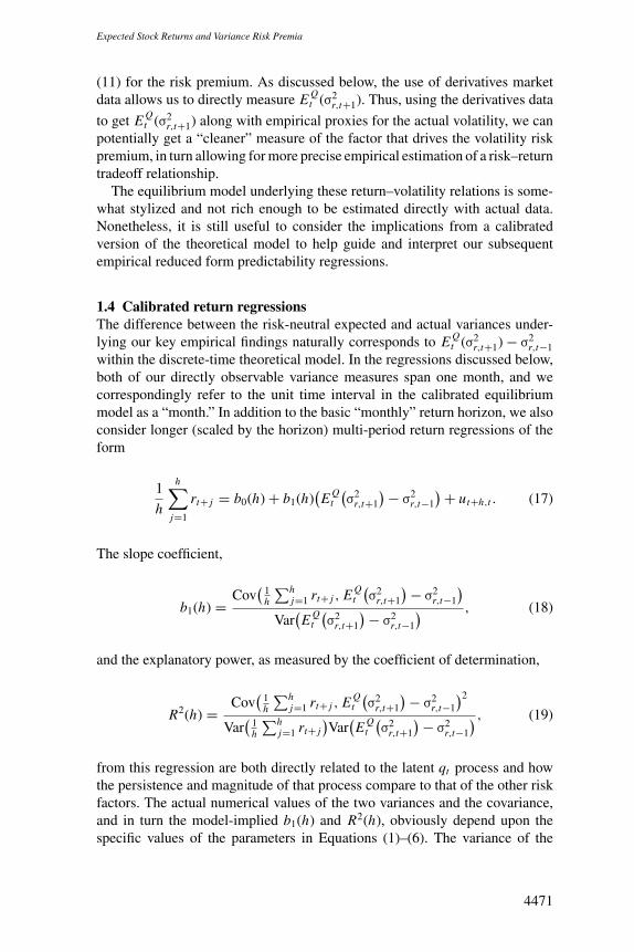
1.4 Calibrated return regressionsThe difference between the risk-neutral expected and actual variances under-lying our key empirical findings naturally corresponds to E Q

t (σ2r,t+1) − σ2

r,t−1within the discrete-time theoretical model. In the regressions discussed below,both of our directly observable variance measures span one month, and wecorrespondingly refer to the unit time interval in the calibrated equilibriummodel as a “month.” In addition to the basic “monthly” return horizon, we alsoconsider longer (scaled by the horizon) multi-period return regressions of theform

1

h

h∑j=1

rt+ j = b0(h) + b1(h)(E Q

t

(σ2

r,t+1

) − σ2r,t−1

) + ut+h,t . (17)

The slope coefficient,

b1(h) = Cov(

1h

∑hj=1 rt+ j , E Q

t

(σ2

r,t+1

) − σ2r,t−1

)Var

(E Q

t

(σ2

r,t+1

) − σ2r,t−1

) , (18)

and the explanatory power, as measured by the coefficient of determination,

R2(h) = Cov(

1h

∑hj=1 rt+ j , E Q

t

(σ2

r,t+1

) − σ2r,t−1

)2

Var(

1h

∑hj=1 rt+ j

)Var

(E Q

t

(σ2

r,t+1

) − σ2r,t−1

) , (19)

from this regression are both directly related to the latent qt process and howthe persistence and magnitude of that process compare to that of the other riskfactors. The actual numerical values of the two variances and the covariance,and in turn the model-implied b1(h) and R2(h), obviously depend upon thespecific values of the parameters in Equations (1)–(6). The variance of the

4471


2 4 6 8 10 12 14 16 18 20 22 240

0.05

0.1

0.15

0.2

0.25

0.3

0.35

0.4

0.45Model−implied slope coefficient

Horizon (months)

Model AModel BModel CModel D

2 4 6 8 10 12 14 16 18 20 22 240

1

2

3

4

5

6Model−implied R−square (%)

Horizon (months)

Model AModel BModel CModel D

Figure 1Model-implied slopes and R2sThe figure shows the population slope coefficients and R2s from regressions of the scaled h-period returns onthe variance difference implied by the equilibrium model. The four different lines refer to the four differentparameter configurations discussed in the main text.

multi-period returns and the covariance of those returns with the variancepremium furthermore depend nontrivially on the return horizon, h.15

To gauge more directly how the predictability varies with the model pa-rameters and h, we plot in Figure 1 the population b1(h)’s and R2(h)’s for

15 Tedious calculations yield

R2(h) =(

1 − θ

θAq (1 − κ1ρq )κ1

[(1 − γ)2

2(1 − κ1ρσ)+ 2A2

qϕ2q (1 − κ1ρq )

]Varq

1 − ρhq

1 − ρq

)2

×[(

θ − 1

θκ1

)2 [(1 − γ)2

2(1 − κ1ρσ)+ 2A2

qϕ2q (1 − κ1ρq )

]2

Varq +(

1 − ρ2q

)Varq +

(1 − ρ2

σ

)Varσ2

g

]−1

×[

haq

1 − ρσ

+[

(1 − κ1)2

(1 − ρσ)2

(h(

1 − ρ2σ

)+ 4ρh+1

σ − 2ρhσ − 2ρ2

σ

)+

(1 − 2ρh

σκ1 + κ21

)]Varσ2

g

+[

(1 − κ1)2

(1 − ρq )2

(h(

1 − ρ2q

)+ 4ρh+1

q − 2ρhq − 2ρ2

q

)+

(1 − 2ρh

qκ1 + κ21

)]Varq

]−1

,

where Varσ2g = aq (1 − ρq )−1(1 − ρ2

σ)−1 and Varq = φ2q aq (1 − ρ2

q )−1(1 − ρ2σ)−1. The corresponding formula for

the slope coefficient b1(h) follows readily from this expression.

4472


four different parameter configurations and return horizons ranging from “onemonth” (h = 1) to “two years” (h = 24). The values for δ = 0.997, γ = 10.0,ψ = 1.5, μg = 0.0015, and E(σg) = 0.0078 in the baseline model (Model A)are all adapted directly from Bansal and Yaron (2004). Additionally, we fixκ1 = 0.9, the persistence of the variance at ρσ = 0.978, the persistence ofthe volatility-of-volatility at ρq = 0.8, the expected volatility-of-volatility ataq (1 − ρq )−1 = 10.0−6, and the volatility of that process at φq = 10.0−3. Themean annualized risk-free rate and equity premium implied by these particularmodel parameters equal 0.69% and 7.79%, respectively.

The model-implied slope coefficients depicted in the top panel of Figure 1all decline monotonically with the return horizon. For the baseline model(Model A), b1(h) starts out at 0.26 declining to 0.10 at the annual horizon.Decreasing (increasing) the persistence in the qt process from ρq = 0.8 to0.6 (0.95), keeping all of the other model parameters the same as in Model B(Model C) results in systematically lower (higher) population slope coefficients.Increasing the value of the intertemporal elasticity of substitution from ψ = 1.5to 2.5 (Model D) magnifies the relation between the returns and the variance riskpremium and results in systematically higher b1(h)’s across all return horizons.

Turning to the model-implied R2(h)’s depicted in the bottom panel in thefigure, the degree of predictability for the baseline model (Model A) starts outfairly low at the “monthly” horizon, rising to its maximum around a “quar-ter,” gradually tapering off thereafter for longer return horizons. In line withthe results for the slope coefficients, lowering the degree of persistence in theqt process to ρq = 0.6 (Model B) results in substantially lower overall pre-dictability, and also shifts the peak in the R2(h)’s from a “quarter” to “twomonths.” Conversely, increasing the persistence to ρq = 0.95 (Model C) in-creases the relative importance of stochastically varying volatility-of-volatilityand prolongs the inherent return predictability. Lastly, changing the value ofthe intertemporal elasticity of substitution from ψ = 1.5 to 2.5 (Model D) en-hances the importance of time-varying volatility-of-volatility and increases theR2(h)’s relative to those for the baseline model (Model A), with the maximumagain occurring around the “quarterly” return horizon.

As these calibrations make clear, the simple stylized general equilibriummodel can give rise to quite sizable regression coefficients and return pre-dictability. Importantly, the calibrations also reveal a general hump shape inthe implied R2 as a function of the return horizon with the location of thepeak directly related to the value of ρq . At an intuitive level, the variancerisk premium or the “variance swap” on the right-hand side of the regression,E Q

t (σ2r,t+1) − σ2

r,t−1, may be seen as a pure volatility bet where everythingelse gets “risk neutralized” out. Since volatility is explicitly priced under theEpstein–Zin–Weil recursive preference structure, this variance difference earnsexactly that volatility risk premium and nothing else. The price of this riskchanges if the variance of the priced factor changes. But this corresponds ex-actly to the volatility-of-volatility or the qt process within the theoretical model.

4473


We next turn to a discussion of the procedures and data that we actually usein empirically quantifying the E Q

t (σ2r,t+1) and σ2

r,t variance measures.

2. Empirical Measurements

The theoretical model outlined in the previous section suggests that the differ-ence between current return variation and the market’s risk-neutral expectationof future return variation may serve as a useful predictor for the future returnsby effectively isolating the systematic risk associated with the volatility-of-volatility. To measure the variance risk premium and investigate this conjecture,we rely on two relatively new nonparametric “model-free” variation concepts.

2.1 Model-free variation measuresTo formally define the procedure that we use in quantifying the market’s ex-pected return variation, let Ct (T, K ) denote the price of a European call optionmaturing at time T with strike price K , and let B(t, T ) denote the price of a timet zero-coupon bond maturing at time T . As shown by Carr and Madan (1998);Demeterfi et al. (1999); and Britten-Jones and Neuberger (2000), the market’srisk-neutral expectation of the total return variation between time t and t + 1conditional on time t information, or the implied variance IVt , may then beexpressed in a “model-free” fashion as the following portfolio of Europeancalls:

IVt ≡ 2∫ ∞

0

Ct(t + 1, K

B(t,t+1)

) − Ct (t, K )

K 2d K

= E Qt [Return variation(t, t + 1)], (20)

which relies on an ever-increasing number of calls with strikes spanning zeroto infinity.16 This “model-free” measure therefore provides a natural empiri-cal analog to E Q

t (σ2r,t+1) in the discrete-time model discussed in the previous

section. In practice, of course, IVt must be constructed on the basis of a fi-nite number of strikes. Fortunately, even with relatively few different options,this tends to provide a fairly accurate approximation to the true (unobserved)risk-neutral expectation of the future return variation, and, in particular, amuch better approximation than the one based on inversion of the standardBlack–Scholes formula with close to at-the-money option(s) (see, for example,Jiang and Tian 2005; Bollerslev, Gibson, and Zhou 2006).

In order to define the measure that we use in quantifying the actual returnvariation, let pt denote the logarithmic price of the asset. The realized variationover the discrete t − 1 to t time interval may then be measured in a “model-free”

16 See Bondarenko (2004); Jiang and Tian (2005); and Carr and Wu (2009) for justification under the assumptionof general jump-diffusion processes.

4474


fashion by

RVt ≡n∑

j=1

[pt−1+ j

n− pt−1+ j−1

n (�)

]2 −→ Return variation(t − 1, t), (21)

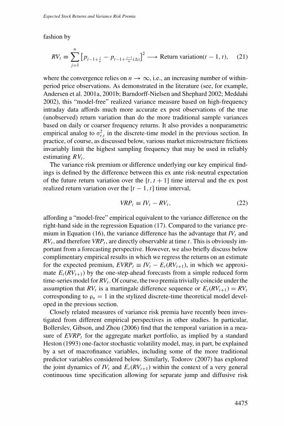
where the convergence relies on n → ∞, i.e., an increasing number of within-period price observations. As demonstrated in the literature (see, for example,Andersen et al. 2001a, 2001b; Barndorff-Nielsen and Shephard 2002; Meddahi2002), this “model-free” realized variance measure based on high-frequencyintraday data affords much more accurate ex post observations of the true(unobserved) return variation than do the more traditional sample variancesbased on daily or coarser frequency returns. It also provides a nonparametricempirical analog to σ2

r,t in the discrete-time model in the previous section. Inpractice, of course, as discussed below, various market microstructure frictionsinvariably limit the highest sampling frequency that may be used in reliablyestimating RVt .

The variance risk premium or difference underlying our key empirical find-ings is defined by the difference between this ex ante risk-neutral expectationof the future return variation over the [t, t + 1] time interval and the ex postrealized return variation over the [t − 1, t] time interval,

VRPt ≡ IVt − RVt , (22)

affording a “model-free” empirical equivalent to the variance difference on theright-hand side in the regression Equation (17). Compared to the variance pre-mium in Equation (16), the variance difference has the advantage that IVt andRVt , and therefore VRPt , are directly observable at time t . This is obviously im-portant from a forecasting perspective. However, we also briefly discuss belowcomplimentary empirical results in which we regress the returns on an estimatefor the expected premium, EVRPt ≡ IVt − Et (RVt+1), in which we approxi-mate Et (RVt+1) by the one-step-ahead forecasts from a simple reduced formtime-series model for RVt . Of course, the two premia trivially coincide under theassumption that RVt is a martingale difference sequence or Et (RVt+1) = RVt

corresponding to ρσ = 1 in the stylized discrete-time theoretical model devel-oped in the previous section.

Closely related measures of variance risk premia have recently been inves-tigated from different empirical perspectives in other studies. In particular,Bollerslev, Gibson, and Zhou (2006) find that the temporal variation in a mea-sure of EVRPt for the aggregate market portfolio, as implied by a standardHeston (1993) one-factor stochastic volatility model, may, in part, be explainedby a set of macrofinance variables, including some of the more traditionalpredictor variables considered below. Similarly, Todorov (2007) has exploredthe joint dynamics of IVt and Et (RVt+1) within the context of a very generalcontinuous time specification allowing for separate jump and diffusive risk

4475


premiums. The difference between implied and realized variance measures hasalso previously been associated empirically with notions of aggregate marketrisk aversion by Rosenberg and Engle (2002), while Bakshi and Madan (2006)have formally shown that the volatility spread may be expressed as a nonlinearfunction of the aggregate degree of risk aversion in a simple representativeagent setting.

2.2 Data descriptionOur empirical analysis is based on the aggregate S&P 500 composite indexas a proxy for the aggregate market portfolio. Due to the dual requirements ofreliable high-frequency data and options-implied volatilities, our sample “only”spans the period from January 1990 to December 2007.

We rely on monthly data for the “new” VIX index for quantifying IVt .The VIX index is based on the highly liquid S&P 500 index options alongwith the “model-free” approach discussed above explicitly tailored to replicatethe risk-neutral variance of a fixed 30-day maturity. The data are obtaineddirectly from the Chicago Board of Options Exchange (CBOE).17 The VIXindex is invariably subject to some approximation error (see, for example, thediscussion in Jiang and Tian 2007), but the CBOE procedure for calculatingthe VIX has arguably emerged as the industry standard. Thus, in order tofacilitate replication and comparison with other studies, we purposely rely onthe readily available squared VIX index as our measure for the risk-neutralexpected variance.

The intraday data for the S&P 500 composite index that we use in theconstruction of our “model-free” RVt measure is provided by the Institute ofFinancial Markets. The theory behind the realized variation measures dictatesthat the sampling frequency, or n in the expression for RVt above, goes toinfinity. However, a host of practical market microstructure features, includingprice discreteness, bid–ask spreads, and nonsynchronous trading effects, implythat the underlying semimartingale assumption for the returns is violated at thevery highest sampling frequencies. In practice, it therefore becomes necessaryto strike a balance between the desire to use very finely sampled data tominimize the estimation error on the one hand and not be overwhelmed by“noise” in the high-frequency prices on the other. A number of studies, usingthe volatility signature plot first proposed by Andersen et al. (2000), suggestthat for highly liquid assets, such as the S&P 500 index analyzed here, a five-minute sampling frequency provides a reasonable choice (see, for example, thediscussion in Hansen and Lunde 2006). Following this recommendation, webase our monthly realized variance measure for the S&P 500 on the summation

17 The CBOE replaced the “old” VIX index, based on S&P 100 options and Black–Scholes implied volatilities,with the “new” VIX index based on S&P 500 options and “model-free” implied volatilities in September 2003.Historical data on both indexes are available from the official CBOE Web site. A more detailed description ofthe procedure actually used in approximating the integral in the calculation of the VIX is provided in the WhitePaper on the CBOE Web site.

4476


Jan 90 Jan 92 Jan 94 Jan 96 Jan 98 Jan 00 Jan 02 Jan 04 Jan 060

50

100

150

S&P 500 implied variance


50

100

150

S&P 500 realized variance


−20

020

40

60

80

100

120Difference between implied and realized variances

Figure 2Implied and realized variances and variance risk premiumThis figure plots the implied variance (the top panel), the realized variance (the middle panel), and the difference(the bottom panel) for the S&P 500 market index from January 1990 to December 2007. The shaded areasrepresent NBER recessions.

of the 78 within-day five-minute squared returns covering the normal tradinghours from 9:30 am to 4:00 pm along with the close-to-open overnight return.18

For a typical month with 22 trading days, this leaves us with a total of n =22 × 78 = 1716 “five-minute” returns.

To illustrate the data, Figure 2 plots the monthly time series of impliedvariances, realized variances, and their differences. Both of the variance mea-sures are somewhat higher during the 1997–2002 part of the sample. The moredistinct spikes in the measures generally also coincide. Consistent with thetheoretical model developed in the previous section and the earlier empiricalevidence cited above, the spread between the implied and realized variances isalmost always positive.

18 Recent studies (for example, Zhang, Mykland, and Aıt-Sahalia 2005; Barndorff-Nielsen et al. 2008) haveproposed more efficient and complicated ways in which to accommodate the market microstructure effects thatallow for finer sampling. However, the simple-to-implement RVt estimator based on the summation of (not toofinely sampled) high-frequency squared returns that we rely on here remains the dominant method in practicalapplications.

4477


Table 1Summary statistics

Rmt − R f t IVt − RVt IVt RVt log(Pt /Et ) log(Pt /Dt ) DFSPt TMSPt RRELt CAYt

Summary statisticsMean 6.44 18.30 33.23 14.93 3.13 3.92 0.84 1.69 −0.11 0.33Std. dev. 47.19 15.13 23.73 15.25 0.26 0.34 0.20 1.19 0.78 1.80Skewness −0.65 2.14 2.02 2.72 0.42 −0.19 0.90 0.09 −0.35 −0.09Kurtosis 4.38 12.06 9.11 12.98 2.44 1.98 3.28 1.79 2.75 1.94AR(1) −0.03 0.49 0.79 0.70 0.97 0.99 0.94 0.98 0.94 0.96

Correlation matrixRmt − R f t 1.00 −0.30 −0.34 −0.23 −0.08 −0.07 −0.05 −0.02 0.00 −0.05IVt − RVt 1.00 0.78 0.22 0.19 0.11 0.10 −0.08 −0.27 −0.04IVt 1.00 0.78 0.41 0.35 0.26 −0.14 −0.31 −0.21RVt 1.00 0.45 0.44 0.31 −0.14 −0.21 −0.30log(Pt /Et ) 1.00 0.65 0.25 0.29 −0.24 −0.59log(Pt /Dt ) 1.00 −0.03 −0.36 0.09 −0.87DFSPt 1.00 0.21 −0.43 −0.03TMSPt 1.00 −0.36 0.35RRELt 1.00 −0.18CAYt 1.00

The sample period extends from January 1990 to December 2007. All variables are reported in annualizedpercentage form whenever appropriate. The Rmt − R f t denotes the logarithmic return on the S&P 500 in excess ofthe three-month T-bill rate. IVt denotes the “model-free” implied variance or VIX index. RVt refers to the “model-free” realized variance constructed from high-frequency five-minute returns. The predictor variables include theprice–earning ratio log(Pt /Et ), the price–dividend ratio log(Pt /Dt ), the default spread DFSPt defined as thedifference between Moody’s BAA and AAA bond yield indices, the term spread TMSPt defined as the differencebetween the ten-year and three-month Treasury yields, and the stochastically detrended risk-free rate RRELt

defined as the one-month T-bill rate minus its trailing twelve-month moving averages. Monthly observations onthe consumption–wealth ratio CAYt are defined by the most recently available quarterly observations.

In addition to the variance risk premium, we also consider a set of othermore traditional predictor variables (see, for example, Lamont 1998; Lettauand Ludvigson 2001; Ang and Bekaert 2007). Specifically, we obtain monthlyP/E ratios and dividend yields for the S&P 500 directly from Standard &Poor’s. Data on the three-month T-bill, the default spread (between Moody’sBAA and AAA corporate bond spreads), the term spread (between the ten-yearT-bond and the three-month T-bill yields), and the stochastically detrended risk-free rate (the one-month T-bill rate minus its backward twelve-month movingaverages) are taken from the public Web site of the Federal Reserve Bank ofSt. Louis. The CAY as defined in Lettau and Ludvigson (2001) is downloadedfrom Lettau and Ludvigson’s Web site.19

Basic summary statistics for the monthly returns and predictor variables aregiven in Table 1. The mean excess return on the S&P 500 over the sample equals6.44% annually. The sample means for the implied and realized variances are33.23 and 14.93, respectively, corresponding to a variance risk premium of18.30 (in percentages squared). The numbers for the traditional forecastingvariables are all directly in line with those reported in previous studies. In par-ticular, all of the variables are highly persistent with first-order autocorrelationsranging from 0.94 to 0.99. In contrast, the serial correlation in the implied and

19 We define a monthly CAY series from the most recent quarterly observation.

4478


realized variances equal 0.79 and 0.70, respectively, and the first-order autocor-relation for their difference only equals 0.49. As such, this alleviates one of thecommon concerns related to the use of highly persistent predictor variables andthe possibility of spurious or unbalanced regressions.20 Anticipating some ofthe results discussed next, the traditional predictor variables all correlate fairlyweakly with the contemporaneous monthly excess returns, while the samplecorrelations between the monthly returns and the different variance measuresare much higher (in an absolute sense), ranging from −0.34 to −0.23.

3. Forecasting Stock Market Returns

All of our forecasts are based on simple linear regressions of the S&P 500excess returns on different sets of lagged predictor variables. We always relyon monthly observations. All of the reported t-statistics are based on het-eroskedasticity and serial correlation consistent standard errors that explicitlytake account of the overlap in the regressions following Hodrick (1992).21 Wefocus our discussion on the estimated slope coefficients and their statisticalsignificance as determined by the robust t-statistics. We also report the fore-casts’ accuracy of the regressions as measured by the corresponding adjustedR2s. However, as previously noted, for the more traditional highly persistentpredictor variables, the R2s for the overlapping multi-period return regressionsneed to be interpreted with great caution.22

3.1 Main empirical findingsWe begin by reporting in Table 2 the results for our empirical equivalent tothe key return regression defined in Equation (17). The degree of predictabilitystarts out fairly low at the monthly horizon with an R2 of just above 1%.The robust t-statistic for testing the estimated slope coefficient associated withthe variance difference IV − RV greater than zero still exceeds the one-sided5% significance level. The quarterly return regression results in a much moreimpressive t-statistic of 2.86 and a corresponding R2 of 6.82%. The t-statisticremains significant at the six-month horizon, but the numerical values andsignificance then gradually taper off for longer return horizons.

20 Inference issues related to the use of highly persistent predictor variables have been studied extensively in theliterature (see, for example, Stambaugh 1999; Ferson, Sarkissian, and Simin 2003; Lewellen 2004; Campbelland Yogo 2006 and references therein). Some authors have gone as far as to attribute the apparent predictabilityto the use of strongly serially correlated predictor variables (for example, Boudoukh, Richardson, and Whitelaw2008; Goyal and Welch 2003, 2008).

21 Ang and Bekaert (2007) have forcefully shown that in the context of predictive regressions with overlappingobservations, the standard errors obtained by summing the regressors in the past, as advocated by Hodrick (1992),are generally more reliable than the more traditional standard errors based on the summation of the residuals intothe future as in, for example, Newey and West (1987).

22 Boudoukh, Richardson, and Whitelaw (2008) have recently shown that even in the absence of any increase inthe true predictability, the values of the R2s with highly persistent predictor variables and overlapping returnswill by construction increase roughly proportional with the return horizon and the length of the overlap (see alsoKirby 1997).

4479


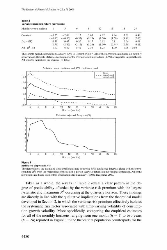
Table 2Variance premium return regressions

Monthly return horizon 1 3 6 9 12 15 18 24

Constant −0.55 −2.08 1.12 3.63 4.62 4.84 5.61 6.48(−0.13) (−0.56) (0.33) (1.15) (1.50) (1.59) (1.81) (2.07)

IVt − RVt 0.39 0.47 0.30 0.17 0.12 0.11 0.06 0.01(1.76) (2.86) (2.15) (1.36) (1.00) (0.94) (0.56) (0.11)

Adj. R2 (%) 1.07 6.82 5.42 2.30 1.23 1.00 0.05 -0.50

The sample period extends from January 1990 to December 2007. All of the regressions are based on monthlyobservations. Robust t-statistics accounting for the overlap following Hodrick (1992) are reported in parentheses.All variable definitions are identical to Table 1.

2 4 6 8 10 12 14 16 18 20 22 24−0.2

0

0.2

0.4

0.6

0.8

Estimated slope coefficient and 95% confidence band

Horizon (months)

SlopeUpper boundLower bound

2 4 6 8 10 12 14 16 18 20 22 24

0

1

2

3

4

5

6

7

8Estimated adjusted R−square (%)

Horizon (months)

Figure 3Estimated slopes and R2sThe figure shows the estimated slope coefficients and pointwise 95% confidence intervals along with the corre-sponding R2s from the regressions of the scaled h-period S&P 500 returns on the variance difference. All of theregressions are based on monthly observations from January 1990 to December 2007.

Taken as a whole, the results in Table 2 reveal a clear pattern in the de-gree of predictability afforded by the variance risk premium with the largestt-statistic and maximum R2 occurring at the quarterly horizon. These findingsare directly in line with the qualitative implications from the theoretical modeldeveloped in Section 2, in which the variance risk premium effectively isolatesthe systematic risk factor associated with time-varying volatility of consump-tion growth volatility. More specifically, comparing the empirical estimatesfor all of the monthly horizons ranging from one month (h = 1) to two years(h = 24) reported in Figure 3 to the theoretical population counterparts for the

4480


four benchmark models depicted in Figure 1, the similarities in the generalshapes of the estimated and implied slope coefficients and R2s as a functionof the return horizon are quite striking. Of course, the values of the R2s at theintermediate three-to six-month horizon for the actual return regressions areslightly larger than the R2s for any of the calibrated models, suggesting thatadditional systematic risk factors, temporal variation in the degree of risk aver-sion, and/or the influence of period-specific idiosyncratic events are needed tofully explain the empirical results.

To better appreciate the findings in a wider empirical context, Tables 3–5report the results from comparable monthly, quarterly, and annual returnregressions, respectively, involving the more traditional predictor variables inTable 1.23 Not surprisingly, the degree of predictability at the monthly horizonis systematically very low, although the individual regressions for both theP/E ratio and CAY do result in t-statistics slightly above two (numerically).24

Combining the variance difference with the P/E ratio results in a monthly R2

of 3.77%, in excess of the sum of the two R2s from the individual regressions.Both of the coefficients also remain statistically significant in the joint regres-sion. Adding the term spread (TMSP) and the relative risk-free rate (RREL)to the multiple regression actually reduces the (adjusted) R2, but the variancepremium remains statistically significant.

The quarterly regressions reported in Table 4 further underscore the signif-icance of the result in Table 2. None of the t-statistics for any of the otherpredictor variables come close to the aforementioned t-statistic for the vari-ance premium (2.86), and with the possible exception of P/E (−1.97) and CAY(1.78), all are insignificant at conventional levels. Of course, the R2s for someof the other predictor variables, most notably the P/E and P/D ratios and CAY,are fairly close to the R2 for the variance premium. However, whereas themonthly variance premium exhibits relatively weak serial correlation, all ofthese other predictor variables are close to unit root-type processes, which aspreviously noted renders the R2s based on overlapping regressions difficult tointerpret.

Turning to the multiple regressions reported in the right panel of Table 4,we find that combining the variance premium with the P/E ratio results ineven more impressive t-statistics of 3.43 and −2.42, respectively. Intuitively,the variance risk premium and the P/E ratio may jointly capture important

23 For comparability with the other slope coefficients, the P/E, P/D, and DFSP variables have been scaled by afactor of 12. Many other predictor variables have, of course, been proposed in the literature. While it is literallyimpossible to investigate all of these suggestions, we also experimented with the bond factor of Cochrane andPiazzesi (2005), but found that it offered little predictability over the 1990–2007 sample period. Similarly, returnregressions based on the corporate payout ratio (D/E) resulted in a negative adjusted R2 over the present sample.

24 By estimating the cointegrating relationship in-sample, the traditional CAY variable suffers from a “look-ahead”bias. Brennan and Xia (2005) argue that this “explains” most of the predictability afforded by CAY. Also, onimplementing the aforementioned adjustment in Stambaugh (1986, 1999) to take account of the finite-samplebias in the estimated coefficients due to the serial correlation in the regressors, the adjustment term for IVt − RVt

equals 0.02, compared to 0.52 and 0.51 for P/E and CAY, respectively. These latter large adjustments are directlyin line with the numbers reported in the extant literature.

4481

The

Review

ofFinancialStudies

/v22

n11

2009

Table 3Monthly return regressions

Simple Multiple

Constant −0.55 −0.19 4.88 92.72 75.51 14.23 7.73 6.67 5.45 101.13 −2.52 78.02 91.20 101.86(−0.13) (−0.04) (1.20) (2.22) (1.87) (0.91) (1.32) (2.12) (1.53) (2.42) (−0.55) (1.49) (1.74) (2.28)

IVt − RVt 0.39 0.49 0.42 0.50 0.57(1.76) (2.16) (1.87) (2.10) (2.34)

IVt 0.20(1.30)

RVt 0.11(0.41)

log(Pt /Et ) −2.30 −2.76 −1.90 −2.49 −2.93(−2.02) (−2.40) (−1.36) (−1.76) (−2.31)

log(Pt /Dt ) −1.47(−1.68)

DFSPt −0.77(−0.50)

TMSPt −0.72 2.87(−0.28) (0.96)

RRELt 1.63 3.29(0.43) (0.76)

CAYt 3.71 3.94 1.78 1.46(2.04) (2.20) (0.87) (0.72)

Adj. R2 (%) 1.07 0.57 −0.34 1.80 1.11 −0.31 −0.43 −0.40 1.44 3.77 2.78 1.89 3.86 3.34

The sample period extends from January 1990 to December 2007. Robust t-statistics following Hodrick (1992) are reported in parentheses. All variable definitions are identical to Table 1,except for P/E, P/D, and DFSP, which have been scaled by a factor of 12.

4482

Expected

StockR

eturnsand

VarianceR

iskP

remia

Table 4Quarterly return regressions

Simple Multiple

Constant −2.08 0.24 6.60 92.41 73.35 20.63 7.39 6.92 5.53 101.89 −4.12 85.93 100.06 98.21(−0.56) (0.06) (1.60) (2.17) (1.81) (1.32) (1.24) (2.18) (1.54) (2.40) (−1.00) (1.67) (1.93) (2.18)

IVt − RVt 0.47 0.58 0.51 0.59 0.70(2.86) (3.43) (3.02) (3.38) (4.01)

IVt 0.19(1.41)

RVt 0.00(0.00)

log(Pt /Et ) −2.28 −2.82 −2.11 −2.77 −2.95(−1.97) (−2.42) (−1.54) (−1.98) (−2.33)

log(Pt /Dt ) −1.42(−1.62)

DFSPt −1.39(−0.90)

TMSPt −0.46 4.08(−0.17) (1.42)

RRELt 3.27 6.39(0.88) (1.56)

CAYt 3.23 3.52 1.08 0.74(1.78) (1.99) (0.53) (0.37)

Adj. R2 (%) 6.82 2.49 −0.47 6.55 4.19 1.18 −0.43 0.43 4.13 16.76 11.87 7.21 17.42 19.74

The sample period extends from January 1990 to December 2007. All of the regressions are based on overlapping monthly observations. Robust t-statistics accounting for the overlapfollowing Hodrick (1992) are reported in parentheses. All variable definitions are identical to Tables 1 and 3.

4483

The

Review

ofFinancialStudies

/v22

n11

2009

Table 5Annual return regressions

Simple Multiple

Constant 4.62 7.62 9.49 78.47 79.83 15.59 5.37 7.29 5.42 81.00 1.91 52.85 55.11 74.04(1.50) (2.44) (3.20) (2.05) (2.17) (1.13) (0.90) (2.33) (1.47) (2.15) (0.53) (1.03) (1.08) (1.88)

IVt − RVt 0.12 0.19 0.18 0.20 0.33(1.00) (1.68) (1.51) (1.74) (2.96)

IVt −0.02(−0.21)

RVt −0.17(−1.20)

log(Pt /Et ) −1.90 −2.06 −1.24 −1.40 −2.14(−1.80) (−2.00) (−0.91) (−1.03) (−1.92)

log(Pt /Dt ) −1.55(−1.92)

DFSPt −0.87(−0.64)

TMSPt 0.88 4.53(0.35) (1.69)

RRELt 4.09 6.29(1.11) (1.75)

CAYt 3.48 3.62 2.13 2.12(1.99) (2.12) (0.99) (0.99)

Adj. R2 (%) 1.23 −0.37 2.89 16.34 19.53 1.79 0.01 4.54 18.15 20.12 21.18 21.46 25.52 32.58

The sample period extends from January 1990 to December 2007. All of the regressions are based on overlapping monthly observations. Robust t-statistics accounting for the overlapfollowing Hodrick (1992) are reported in parentheses. All variable definitions are identical to Tables 1 and 3.

4484


short- and long-run risks embedded in the market returns. This would also beconsistent with the qualitative implications from a more elaborate equilibriummodel combining the model in Section 2 with the long-run risk model ofBansal and Yaron (2004), allowing for time-varying volatility and volatility-of-volatility as well as predictability in the mean of consumption growth. Asimilar empirical pattern, albeit to a lesser extent, obtains when including theCAY variable along with the variance premium, resulting in t-statistics of 3.02and 1.99, respectively. On the other hand, combining the P/E ratio and CAYin the same quarterly return regressions results in insignificant t-statistics forboth. Even though the term spread and the relative short rate are insignificant bythemselves, both variables contribute marginally to a joint predictive regressionwith the variance premium and the P/E ratio, resulting in the highest overalladjusted R2 in the table. Lastly, it is worth noting that regardless of the othervariables included in the forecast regressions, the estimated coefficients for thevariance risk premium remain quite stable and statistically significant at the0.001 level or better.

Many of the empirical studies cited above have, of course, argued that thedegree of predictability afforded by the different valuation ratios and predictorvariables included in Table 1 tend to be the strongest over longer multi-yearhorizons. Our limited post-1990 sample prevents us from effectively studyingissues having to do with longer return horizons spanning multiple years. How-ever, we do report in Table 5 the regression results for annual returns basedon monthly overlapping observations, but again caution that with such a shortcalendar time span and large overlap, the estimation results, and especially theR2s, must be carefully interpreted. Indeed, despite the large R2s, the t-statisticsfor P/E, P/D, and CAY are all just barely significant. As before, including thevariance premium with either of these other variables results in larger (in anabsolute sense) t-statistics for both. In parallel to Tables 3 and 4, the overalllargest t-statistic (2.96) is again associated with the variance premium in themultiple regression reported in the last column in the table.

The simple regressions involving RV or IV reported in Tables 3–5 alwaysresult in insignificant t-statistics and low R2s. This is, of course, to be expectedfrom the extant risk–return literature, which has largely searched in vain forsuch a tradeoff relationship. To further explore this issue and the interplaybetween the two volatility measures, we report in Table 6 the results obtainedby including RV and VRP = IV − RV in the same return regressions. Looking atthe quarterly return horizon in the middle part of the table, it is noteworthy thatwhile VRP is highly significant, RV remains insignificant in the joint regression.As such, this implicitly attributes the same numerical but opposite signed effectsto IV and RV. Following the discussion in Section 2, it appears that the variancedifference VRP effectively isolates the factor that drives the volatility riskpremium, thereby allowing for the estimation of a meaningful and significantrisk–return tradeoff relationship. Meanwhile, previous studies in the risk–returnliterature (for example, Scruggs 1998; Guo and Whitelaw 2006) have argued

4485


Table 6Risk–return tradeoff

Monthly returns Quarterly returns Annual returns

Constant −0.83 112.29 134.16 −0.88 113.52 121.71 6.84 78.82 81.17(−0.18) (2.88) (2.85) (−0.21) (2.77) (2.71) (2.22) (2.28) (2.16)

RVt 0.03 0.32 0.46 −0.11 0.17 0.33 −0.22 −0.03 0.10(0.10) (1.22) (1.58) (−0.41) (0.65) (1.11) (−1.25) (−0.23) (0.75)

IVt − RVt 0.38 0.45 0.54 0.50 0.56 0.69 0.17 0.20 0.33(1.68) (2.02) (2.43) (2.91) (3.42) (4.22) (1.43) (1.73) (2.94)

log(Pt /Et ) −3.43 −4.06 −3.18 −3.76 −1.99 −2.39(−2.91) (−2.93) (−2.80) (−2.87) (−2.13) (−2.23)

TMSPt 4.95 5.52 4.97(1.48) (1.68) (1.82)

RRELt 5.09 7.55 6.62(1.17) (1.82) (1.87)

Adj. R2 (%) 0.61 4.17 4.45 6.78 17.11 21.81 5.80 19.80 33.00

The sample period extends from January 1990 to December 2007. All of the regressions are run at a monthlyfrequency. Robust t-statistics accounting for the overlap following Hodrick (1992) are reported in parentheses.All variable definitions are identical to Tables 1 and 3.

that additional control factors, including interest rates, are needed in orderto reliably estimate the relationship between expected return and volatility.25

To investigate this, we include the P/E ratio, the term spread, and the shortrate in the return regressions. This only reinforces the superior predictabilityafforded by the variance premium. Whereas many of the t-statistics for thevariance premium (all at the quarterly horizon) are highly significant, none ofthe t-statistics associated with RV and the more traditional risk–return tradeoffestimated in the literature are significant.

3.2 Other variation measuresThe regression results discussed above were directly motivated by the stylizedequilibrium model in Section 2, in which the dynamics were cast in varianceform, and in which the different variation measures were approximated empiri-cally by their “model-free” counterparts. We next discuss a series of additionalreturn regressions and sensitivity checks based on other variation measuresand volatility transforms designed to address the robustness and validity ofour findings in a wider sense. To conserve space, we will focus our summarydiscussion on the quarterly return horizon that produced the most significantresults. Also, we do not include any additional tables, but more detailed tabularinformation related to these results is available upon request.

3.2.1 “Old” variance measures. The “model-free” implied and realizedvariances underlying our empirical results are both relatively new. As a firstrobustness check, we replace the “model-free” variance measures with thestandard at-the-money Black–Scholes implied variance IV∗, and the realized

25 With higher interest rates generally associated with more turbulent financial markets, this may also be seen asproxying for the qt process in the stylized equilibrium model.

4486


variance based on low-frequency daily returns RV∗. Interestingly, the regres-sions based on these “old” variance measures generally do not give rise tothe same strong conclusions. The variance risk premium defined by the differ-ence between the Black–Scholes implied variance and the daily return basedrealized variance still dominates each of the variance measures in isolationwith t-statistics of 1.72 versus 0.97 and 0.31, respectively. However, the R2

for the “model-free” variance premium in Table 4 (6.82%) is much larger thanthe 2.16% obtained with the difference between the “old” variance measures.Replacing the realized variance based on daily data with the correspondinghigh-frequency-based measure results in a marginally significant t-statistic of1.85 and increases the R2 to 3.30%. Similarly, replacing the Black–Scholesimplied variance with the “model-free” implied variance results in a t-statisticof 2.34 and increases the R2 to 4.45%.26

All in all, these results clearly show that our use of the new “model-free”variance measures is crucial in effectively uncovering the variance risk pre-mium. Estimation of the same predictive regressions based on the traditionalBlack–Scholes implied variances and/or realized variances constructed fromlower frequency daily data does not give rise to nearly as significant results.

3.2.2 Volatility risk premia. The regressions discussed so far have all beencast in variance form.27 This, of course, directly mirrors the expressions forthe variance premia and predictability regressions derived within the context ofthe theoretical model in Section 2. However, the volatility, or other nonlinearmonotone transforms of the variance, is often used as an alternative and em-pirically more robust measure of risk (for example, Merton 1980). Replacingthe “model-free” variance measures with their volatility or standard deviationcounterparts yields a t-statistic of 2.75 and an R2 of 6.51% for the volatility dif-ference

√IV − √

RV, compared to 2.86 and 6.82% for the variance differenceIV − RV. Again, including

√IV and

√RV individually results in insignificant

t-statistics of 1.01 and −0.12, respectively. The results for the multiple regres-sions obtained by including the P/E ratio, CAY, and the term structure variablestogether with the volatility difference are comparable to the ones for the vari-ance premium, but all of the t-statistics and R2s fall short of those reported inTable 4.

3.2.3 Expected variation premium. The empirical variance risk premiumdefined in Equation (22) is based on the difference between the market’s (riskneutral) expected variation and the current realized variation. Both of these mea-sures and in turn the premium are directly observable at time t in a completely

26 This indirectly suggests that much of the useful information about the temporal variation in the risk-neutralizedvariance resides in options away from the money.

27 This corresponds to the common use of variance-denominated contracts in the over-the-counter swap market(see, for example, Demeterfi et al. 1999; Mixon 2007).

4487


“model-free” fashion. The resulting regressions with VRP on the right-handside also directly mirror the population regressions analyzed within the styl-ized equilibrium model in Section 2. More generally, however, our empiricalfindings that higher (lower) values of the variance premium are associated withhigher (lower) future returns may, in part, be attributed to the effect that whenthe market anticipates high (low) volatility going forward, there is a discount(premium) built into prices, resulting in high (low) future returns. To moreclearly separate this effect from temporal variation in the volatility risk pre-mium per se, it is useful to consider a regression of the returns on an estimateof the previously defined forward looking,28 or expected, variance premium,EVRPt ≡ IVt − Et (RVt+1).

In contrast to all of the other predictor variables and “model-free” empiricalmeasures considered so far, this necessitates an explicit forecasting model forRVt . Numerous parametric and nonparametric volatility forecasting procedureshave been proposed in the literature (see, for example, Andersen et al. 2006). Wehere rely on the simple-to-implement, yet empirically highly accurate, reducedform HAR-RV model advocated by Corsi (2004) and Andersen, Bollerslev, andDiebold (2007), among others, in which the forecast for the one-month-aheadvolatility is a linear function of the current daily, weekly, and monthly realizedvolatilities. Regressing the quarterly overlapping returns on a constant and thisexpected variance premium results in a t-statistic of 2.27 and an R2 of 4.27.29

Although this t-statistic for EVRP is somewhat lower than the one for VRP(2.86), it is still higher than the t-statistics for any of the other predictor variablesin Table 4. Of course, given the high degree of volatility persistence inherent inthe S&P 500 returns, it is hardly surprising that the expected variance differenceand the directly observable variance difference perform fairly similarly from aforecasting perspective.30

4. Conclusion

We provide empirical evidence that stock market returns are predictable by thedifference between “model-free” implied and realized variances or the variancerisk premium. The results appear remarkably robust across different specifi-cations and/or the inclusion of alternative predictor variables. The degree ofpredictability is the largest at intermediate quarterly horizons, but the premiumstill helps explain the observed return variation at shorter monthly and longerannual horizons. Our empirical findings are broadly consistent with the impli-cations from a simple representative agent economy with recursive preferences

28 Related to this, Ang et al. (2009) rely on forward looking volatility estimates constructed by instrumental variablesprocedures in their analysis of cross-sectional pricing of idiosyncratic volatility.

29 Since our estimation of the HAR-RV model for RVt is based on the full sample, the results are subject to astandard “look-ahead” bias and additional parameter estimation error uncertainty.

30 The sample correlation between EVRP and VRP equals 0.85, which far exceeds that for any other pair of predictorvariables in Table 1.

4488


that explicitly incorporates the equilibrium effects of economic uncertainty andtime-varying volatility-of-volatility, although the magnitudes of the estimatedeffects appear too large to be fully explained by the new stylized theoreticalmodel.

The wedge between the “model-free” risk-neutral expected and actual vari-ance underlying our empirical results may alternatively be seen as a proxyfor the aggregate degree of risk aversion in the market.31 Although it mightbe difficult to contemplate systematic changes in the level of risk aversion atthe frequencies emphasized in our empirical work, time-varying volatility riskand time-varying risk aversion likely both play an important role in explainingtemporal variation in expected returns (for example, Bekaert, Engstrom, andGrenadier 2005; Bekaert, Engstrom, and Xing 2008). Recent work directlymotivated by the empirical results first reported here based on more elaborateequilibrium models (Drechsler and Yaron 2008) and cross-sectional pricingrelations (Nyberg and Wilhelmsson 2007) should prove an important next stepin sorting out these issues and further clarify the economic mechanisms behindthe predictability afforded by the variance risk premium.

ReferencesAıt-Sahalia, Y., and A. W. Lo. 2000. Nonparametric Risk Management and Implied Risk Aversion. Journal ofEconometrics 94:9–51.

Andersen, T. G., T. Bollerslev, P. F. Christoffersen, and F. X. Diebold. 2006. Volatility and Correlation Forecasting.In G. Elliott, C. W. J. Granger, and A. Timmermann (eds.), Handbook of Economic Forecasting, chap. 15,pp. 777–878. Amsterdam: Elsevier.

Andersen, T. G., T. Bollerslev, and F. X. Diebold. 2007. Roughing It Up: Including Jump Components in theMeasurement, Modeling, and Forecasting of Return Volatility. Review of Economics and Statistics 89:701–20.

Andersen, T. G., T. Bollerslev, F. X. Diebold, and H. Ebens. 2001a. The Distribution of Realized Stock ReturnVolatility. Journal of Financial Economics 61:43–76.

Andersen, T. G., T. Bollerslev, F. X. Diebold, and P. Labys. 2000. Great Realizations. Risk 13:105–8.

Andersen, T. G., T. Bollerslev, F. X. Diebold, and P. Labys. 2001b. The Distribution of Realized Exchange RateVolatility. Journal of the American Statistical Association 96:42–55.

Ang, A., and G. Bekaert. 2007. Stock Return Predictability: Is it There? Review of Financial Studies 20:651–707.

Ang, A., R. Hodrick, Y. Xing, and X. Zhang. 2006. The Cross-Section of Volatility and Expected Returns.Journal of Finance 61:259–99.

Ang, A., R. Hodrick, Y. Xing, and X. Zhang. 2009. High Idiosyncratic Volatility and Low Returns: Internationaland Further U.S. Evidence. Journal of Financial Economics 91:1–23.

Ang, A., and J. Liu. 2007. Risk, Return, and Dividends. Journal of Financial Economics 85:138.

Bakshi, G., and D. Madan. 2006. A Theory of Volatility Spread. Management Science 52:1945–56.

31 More complicated model-specific measures of risk aversion based on the information in options prices havepreviously been explored empirically by a number of studies (see, for example, Aıt-Sahalia and Lo 2000;Rosenberg and Engle 2002; Brandt and Wang 2003; Gordon and St-Amour 2004; Wu 2005; Garcia et al. 2006;Ziegler 2007).

4489


Bansal, R., V. Khatchatrian, and A. Yaron. 2005. Interpretable Asset Markets? European Economic Review49:531–60.

Bansal, R., and A. Yaron. 2004. Risks for the Long Run: A Potential Resolution of Asset Pricing Puzzles. Journalof Finance 59:1481–509.

Barndorff-Nielsen, O., and N. Shephard. 2002. Econometric Analysis of Realized Volatility and Its Use inEstimating Stochastic Volatility Models. Journal of Royal Statistical Society, B 64:253–80.

Barndorff-Nielsen, O. E., P. R. Hansen, A. Lunde, and N. Shephard. 2008. Designing Realised Kernels to Measurethe Ex-post Variation of Equity Prices in the Presence of Noise. Econometrica 76:1481–1536.

Beckers, S., and T. Bouten. 2005. Implied Volatility and Market Timing. Finance Letters 3:12–16.

Bekaert, G., E. Engstrom, and S. R. Grenadier. 2005. Stock and Bond Returns with Moody Investors. WorkingPaper, Columbia University.

Bekaert, G., E. Engstrom, and Y. Xing. 2008. Risk, Uncertainty, and Asset Prices. Journal of Financial Economics.

Bekaert, G., and J. Liu. 2004. Conditioning Information and Variance Bounds on Pricing Kernels. Review ofFinancial Studies 17:339–78.

Bollerslev, T., M. Gibson, and H. Zhou. 2006. Dynamic Estimation of Volatility Risk Premia and Investor RiskAversion from Option-Implied and Realized Volatilities. Working Paper, Federal Reserve Board.

Bondarenko, O. 2004. Market Price of Variance Risk and Performance of Hedge Funds. Working Paper, Universityof Illinois.

Boudoukh, J., M. Richardson, and R. F. Whitelaw. 2008. The Myth of Long-Horizon Predictability. Review ofFinancial Studies 21:1577–1605.

Brandt, M. W., and K. Q. Wang. 2003. Time-Varying Risk Aversion and Expected Inflation. Journal of MonetaryEconomics 50:1457–98.

Brennan, M. J., and Y. Xia. 2005. TAY’s as Good as CAY. Finance Research Letters 2:1–14.

Britten-Jones, M., and A. Neuberger. 2000. Option Prices, Implied Price Processes, and Stochastic Volatility.Journal of Finance 55:839–66.

Campbell, J. Y., and R. J. Shiller. 1988. The Dividend–Price Ratio and Expectations of Future Dividends andDiscount Factors. Review of Financial Studies 1(3):195–228.

Campbell, J. Y., and M. Yogo. 2006. Efficient Tests of Stock Return Predictability. Journal of Financial Economics81:27–60.

Carr, P., and D. Madan. 1998. Towards a Theory of Volatility Trading. In R. Jarrow (ed.), Volatility: NewEstimation Techniques for Pricing Derivatives, chap. 29, pp. 417–27. London: Risk Books.

Carr, P., and L. Wu. 2009. Variance Risk Premia. Review of Financial Studies 22.

Cochrane, J. H. 2008. The Dog That Did Not Bark: A Defense of Return Predictability. Review of FinancialStudies 21:1533–75.

Cochrane, J. H., and M. Piazzesi. 2005. Bond Risk Premia. American Economic Review 95:138–60.

Corsi, F. 2004. A Simple Long Memory Model of Realized Volatility. Working Paper, University of SouthernSwitzerland.

Demeterfi, K., E. Derman, M. Kamal, and J. Zou. 1999. A Guide to Volatility and Variance Swaps. Journal ofDerivatives 6:9–32.

Drechsler, I., and A. Yaron. 2008. What’s Vol Got to Do with It. Working Paper, University of Pennsylvania.

Epstein, L. G., and S. E. Zin. 1991. Substitution, Risk Aversion, and the Temporal Behavior of Consumption andAsset Returns: An Empirical Analysis. Journal of Political Economy 99:263–86.

4490


Ferson, W. E., S. Sarkissian, and T. T. Simin. 2003. Spurious Regressions in Financial Economics? Journal ofFinance 58:1393–414.

Garcia, R., M.-A. Lewis, S. Pastorello, and E. Renault. 2006. Estimation of Objective and Risk-Neutral Distri-butions Based on Moments of Integrated Volatility. Working Paper, CRDE, Universite de Montreal.

Gordon, S., and P. St-Amour. 2004. Asset Returns and State-Dependent Risk Preferences. Journal of Businessand Economic Statistics 22:241–52.

Goyal, A., and I. Welch. 2003. Predicting the Equity Premium with Dividend Ratios. Management Science49:639–54.

Goyal, A., and I. Welch. 2008. A Comprehensive Look at the Empirical Performance of Equity PremiumPrediction. Review of Financial Studies 21:1455–1508.

Guo, H., and R. F. Whitelaw. 2006. Uncovering the Risk–Return Relation in the Stock Market. Journal of Finance61:1433–63.

Hansen, P. R., and A. Lunde. 2006. Realized Variance and Market Microstructure Noise. Journal of Businessand Economic Statistics 24:127–61.

Heston, S. 1993. A Closed-Form Solution for Options with Stochastic Volatility with Applications to Bond andCurrency Options. Review of Financial Studies 6:327–43.

Hodrick, R. J. 1992. Dividend Yields and Expected Stock Returns: Alternative Procedures for Inference andMeasurement. Review of Financial Studies 5:357–86.

Hsieh, D. A. 1991. Chaos and Nonlinear Dynamics: Application to Financial Markets. Journal of Finance46:1839–77.

Jiang, G., and Y. Tian. 2005. Model-Free Implied Volatility and Its Information Content. Review of FinancialStudies 18:1305–42.

Jiang, G. J., and Y. S. Tian. 2007. Extracting Model-Free Volatility from Option Prices: An Examination of theVIX Index. Journal of Derivatives 14:1–26.

Kirby, C. 1997. Measuring the Predictable Variation in Stock and Bond Returns. Review of Financial Studies10:579–630.

Kreps, D. M., and E. L. Porteus. 1978. Temporal Resolution of Uncertainty and Dynamic Choice Theory.Econometrica 46:185–200.

Lamont, O. 1998. Earnings and Expected Returns. Journal of Finance 53:1563–87.

Lettau, M., and S. Ludvigson. 2001. Consumption, Aggregate Wealth, and Expected Stock Returns. Journal ofFinance 56:815–49.

Lettau, M., S. Ludvigson, and J. Wachter. 2008. The Declining Equity Premium: What Role Does MacroeconomicRisk Play? Review of Financial Studies 21:1653–87.

Lewellen, J. 2004. Predicting Returns with Financial Ratios. Journal of Financial Economics 74:209–35.

Meddahi, N. 2002. Theoretical Comparison Between Integrated and Realized Volatility. Journal of AppliedEconometrics 17:479–508.

Merton, R. C. 1973. An Intertemporal Capital Asset Pricing Model. Econometrica 41:867–87.

Merton, R. C. 1980. On Estimating the Expected Return on the Market. Journal of Financial Economics 8:323–61.

Mixon, S. 2007. The Implied Volatility Term Structure of Stock Index Options. Journal of Empirical Finance14:333–54.

Newey, W. K., and K. D. West. 1987. A Simple Positive Semi-Definite, Heteroskedasticity and AutocorrelationConsistent Covariance Matrix. Econometrica 55:703–8.

4491


Nyberg, P., and A. Wilhelmsson. 2007. Volatility Risk Premium, Risk Aversion and the Cross-Section of StockReturns. Working Paper, Swedish School of Economics and Business Administration.

Rosenberg, J. V., and R. F. Engle. 2002. Empirical Pricing Kernels. Journal of Financial Economics 64:341–72.

Schwert, G. W. 1990. Stock Volatility and the Crash of ’87. Review of Financial Studies 3:77–102.

Scruggs, J. T. 1998. Resolving the Puzzling Intertemporal Relation Between the Market Risks Premium andConditional Market Variance: A Two-Factor Approach. Journal of Finance 53:575–603.

Stambaugh, R. F. 1986. Bias in Regressions with Lagged Stochastic Regressors. Working Paper, Graduate Schoolof Business, University of Chicago.

Stambaugh, R. F. 1999. Predictive Regressions. Journal of Financial Economics 54:375–421.

Todorov, V. 2007. Variance Risk Premium Dynamics. Working Paper, Northwestern University.

Weil, P. 1989. The Equity Premium Puzzle and the Risk Free Rate Puzzle. Journal of Monetary Economics24:401–21.

Wu, L. 2005. Variance Dynamics: Joint Evidence from Options and High-Frequency Returns. Working Paper,Baruch College at CUNY.

Zhang, L., P. A. Mykland, and Y. Aıt-Sahalia. 2005. A Tale of Two Time Scales: Determining Integrated Volatilitywith Noisy High-Frequency Data. Journal of the American Statistical Association 100:1394–411.

Ziegler, A. 2007. Why Does Implied Risk Aversion Smile? Review of Financial Studies 20:859–904.

4492

Expected Stock Returns and Variance Risk Premiaecon.duke.edu/~boller/Published_Papers/rfs_09.pdf ·...

Documents

Transcript of Expected Stock Returns and Variance Risk Premiaecon.duke.edu/~boller/Published_Papers/rfs_09.pdf ·...