Journal of Computational Physics · a Department of Civil Engineering, University of Salerno, 84084...

Journal of Computational Physics 231 (2012) 528–540

Contents lists available at SciVerse ScienceDirect

Journal of Computational Physics

journal homepage: www.elsevier .com/locate / jcp

On the estimation of the curvatures and bending rigidity ofmembrane networks via a local maximum-entropy approach

F. Fraternali a,b, C.D. Lorenz c, G. Marcelli d,⇑a Department of Civil Engineering, University of Salerno, 84084 Fisciano (SA), Italyb Division of Engineering, King’s College London, Strand, London WC2R 2LS, UKc Department of Physics, King’s College London, Strand, London WC2R 2LS, UKd School of Engineering and Digital Arts, Jennison Building, University of Kent, Canterbury, Kent CT2 7NT, UK

a r t i c l e i n f o

Article history:Received 8 October 2010Received in revised form 2 March 2011Accepted 13 September 2011Available online 1 October 2011

Keywords:Membrane networksPrincipal curvaturesBending rigidityMaximum information entropyMinimum widthRed blood cell membrane

0021-9991/$ - see front matter � 2011 Elsevier Incdoi:10.1016/j.jcp.2011.09.017

⇑ Corresponding author.E-mail addresses: [email protected]

(G. Marcelli).

a b s t r a c t

We present a meshfree method for the curvature estimation of membrane networks basedon the local maximum entropy approach recently presented in [1]. A continuum regulari-zation of the network is carried out by balancing the maximization of the informationentropy corresponding to the nodal data, with the minimization of the total width of theshape functions. The accuracy and convergence properties of the given curvature predic-tion procedure are assessed through numerical applications to benchmark problems,which include coarse grained molecular dynamics simulations of the fluctuations of redblood cell membranes [2,3]. We also provide an energetic discrete-to-continuum approachto the prediction of the zero-temperature bending rigidity of membrane networks, which isbased on the integration of the local curvature estimates. The local maximum entropyapproach is easily applicable to the continuum regularization of fluctuating membranes,and the prediction of membrane and bending elasticities of molecular dynamics models.

� 2011 Elsevier Inc. All rights reserved.

1. Introduction

The estimation of the curvature tensor of membrane networks embedded in the 3D Euclidean space plays a key role inmany relevant problems of differential geometry, solid mechanics, biomechanics, biophysics and computer vision. Particu-larly important is the curvature estimation of fluctuating bio-membranes, which are often modeled as particle networks, viamolecular dynamics (MD) and/or coarse grained molecular dynamics (CGMD) approaches. The plasticity of cellular mem-branes is dependent on accurately selected mechanisms for sensing curvature and adopt different responses according tothe particular membrane curvature. These mechanisms depend on the interplay between proteins and lipids and can bemodulated by changes in lipid composition [4], membrane fusion [5], formation of raft-like domains, oligomerization of scaf-folding proteins and/or insertion of wedge proteins into membranes. The dynamical changes in the membrane curvature cangive rise to cell membrane remodelling [6] resulting in the formation of microenvironments that can facilitate the interactionof biomolecules in the cell. On a larger scale, these dynamical changes play a key role in controlling cellular growth, divisionand movement processes. Furthermore, there has been a significant amount of modeling work focussed on characterizing thebending rigidity of ordered membranes [7], vesicle membranes [8,9] and the red blood cell membrane [2,3,10].

The continuum regularization of a membrane network is naturally performed through meshfree approximation schemes,which are well suited for the discrete-to-continuum scale bridging. Recently, a local maximum entropy (LME) approach has

. All rights reserved.

(F. Fraternali), [email protected] (C.D. Lorenz), [email protected], [email protected]

http://dx.doi.org/10.1016/j.jcp.2011.09.017

mailto:[email protected]




http://dx.doi.org/10.1016/j.jcp.2011.09.017

http://www.sciencedirect.com/science/journal/00219991

http://www.elsevier.com/locate/jcp

F. Fraternali et al. / Journal of Computational Physics 231 (2012) 528–540 529

been proposed to construct smooth meshfree approximants of given nodal data [1,11,12]. The LME approach is a convex,non-interpolant approximation method that suitably balances the maximization of the information entropy correspondingto the given data [13], with the minimization of the total width of the shape functions [14]. Some of the distinctive featuresof such an approach consist of the non-negativity and the partition of unity properties of the shape functions, which in par-ticular can be thought of as the elements of a discrete probability distribution; a weak interpolation (Kronecker-delta) prop-erty at the boundary; and first- or higher-order consistency conditions [1,11]. As compared to popular, ‘explicit’approximation methods, such as approaches utilizing B-Splines and Non-Uniform Rational B-Splines (NURBS), the LME re-quires more calculations and specifically the solution of a convex nonlinear optimization problem at each sampling point.Nevertheless, the LME guarantees high accuracy and smoothness of the continuous mapping [11], which are properties offundamental importance when dealing with curvature estimation. Due to its mixed, local–global character, the LME approx-imation scheme can be conveniently used to filter the inherent small scale roughness of the membrane, which is a distinctivefeature of such an approach, as compared to popular computer graphic methods for estimating the curvatures of point-setsurfaces, (e.g. moving least-squares (MLS) methods). Another peculiar advantage of the LME regularization consists of itsability to handle unstructured node sets, which do not require any special pre-processing in such a scheme An extensivecomparison of the application of the LME, MLS and B-Spline approaches to structural vibration problems is presented in [11].

The present work deals with the formulation and the implementation of a curvature estimation method for membranenetworks, which is based on the LME approach proposed in [1]. In Section 2, we provide the explicit formulae for the sec-ond-order derivatives of the LME shape functions (not given in [1]), and a LME procedure for the estimation of the linesof curvature and the principal curvatures at the generic node of a membrane network. Next, we present in Section 3 somenumerical applications of the above procedure to membrane networks extracted from a sinusoidal surface and a sphericalsurface, establishing comparisons with exact solutions and assessing the convergence properties of the LME estimates.We also provide, in the same section, some numerical results about the principal curvatures of the red blood cell (RBC) modelproposed in [2,3], and a discrete-to-continumm approach to the prediction of the bending rigidity at zero temperature of MDmembrane networks. The method and results presented here represent an essential first step towards an extensive estima-tion of the elastic moduli of the RBC, which will be the specific subject of future studies. Additionally, we plan to use thesame approach to measure from trajectories of coarse-grain MD simulations the curvature of cell membranes affected byasymetric lipid bilayers or by protein-lipids interactions. Such future extensions of the present work are summarized in Sec-tion 4, which also includes some final comments on the results presented in Section 3.

2. LME regularization of membrane networks

2.1. Generalities on the LME approximation

First, we will present how to find the continuum regularization of a given discrete set XN of N nodes (or vertices) havingCartesian coordinates fxa1 ; xa2 ; zag (a = 1, . . . ,N) with respect to a given frame {O,x1,x2,z � x3}. We wish to construct a contin-uum surface described by the Monge chart

z ¼ zNðxÞ ¼XN

a¼1

zapaðxÞ ð1Þ

where pa are suitable shape functions of the position vector x = {x1,x2} in the x1, x2 plane. When adopting the local maximumentropy approach proposed in [1], we determine the functions pa by solving the following optimization problem:

For a given x, we minimize:

fbðx;pÞ � bXN

a¼1

pajx� xaj2 þXN

a¼1

pa log pa ð2Þ

subject to:

pa P 0; a ¼ 1; . . . ;N ð3ÞXN

a¼1

pa ¼ 1 ð4Þ

XN

a¼1

paxa ¼ x ð5Þ

where b 2 [0,+1) is a scalar parameter, and p = {p1, . . . ,pN}. The constraints (3)–(5) enforce the non-negativity of the shapefunctions, the partition of unity property, and the first-order consistency conditions, respectively. It is worth noting that Eqs.(4) and (5) guarantee that affine functions are exactly reproduced by the LME scheme [1,11]. On the other hand, Eqs. (3) and(4) allow us to regard p(x) as a discrete probability distribution, and the quantity HIðpÞ ¼ �

PNa¼1pa log pa as the correspond-

ing information entropy [13]. The quantity WðpÞ ¼PN

a¼1pajx� xaj2 instead represents the total width of the shape functionspa at the given x. Depending on the value of b, the LME problem suitably balances the maximization of the information en-

530 F. Fraternali et al. / Journal of Computational Physics 231 (2012) 528–540

tropy corresponding to the given nodal data with the minimization of the total width of the shape functions pa. A global max-imum-entropy scheme ([13]) is recovered by setting b = 0 in (2), while a minimum-width approximation scheme ([14]) isobtained in the limit b ? +1.

Now, we introduce the partition function Zðx; kÞ ¼PN

a¼1Zaðx; kÞ, where k = {k1,k2} denotes the vector of the Lagrange mul-tipliers of the first-order consistency conditions (5), and it results in

Zaðx; kÞ ¼ exp½�bjx� xaj2 þ k � ðx� xaÞ� ð6Þ

It can be shown ([1]) that, for any x 2 convX, the LME problem admits the unique solution shown below

p�aðxÞ ¼Zaðx; k�ÞZðx; kÞ ð7Þ

where

k� ¼ arg mink2RdfFðkÞ ¼ log Zðx; kÞg ð8Þ

It is useful to the employ the Newton–Raphson method to solve Eq. (8) iteratively. Let kk denote the approximate solution to(8) at the kth iteration. A Newton–Raphson update furnishes

kkþ1 ¼ kk � ðJ�1Þkrk ð9Þ

where rk and JK are the particularization of the gradient r and the Hessian J of F for k = kk. Straightforward calculations (cf. [1])give

rðx; kÞ ¼ rFðkÞ ¼XN

a¼1

1Z@Za

@k¼XN

a¼1

paðx� xaÞ ð10Þ

Jðx; kÞ ¼ r2FðkÞ ¼XN

a¼1

@pa

@k

��x� ðx� xaÞ ¼

XN

a¼1

paðx� xaÞ � ðx� xaÞ � r� r ð11Þ

2.2. Derivatives of the LME shape functions

The analysis carried out in [1] leads to the following expression of the spatial gradient of p�a

rp�a ¼ �p�aðJ�Þ�1ðx� xaÞ ð12Þ

where J⁄ = J(x,k⁄).Now we compute the second-order derivatives of the LME shape functions. Differentiating both sides of (12) once, we get

p�a;ij ¼@2p�a@xi@xj

¼ @

@xj�p�aJ��1

ik ðxk � xakÞ

h i¼ p�a;jJ

��1ik ðxk � xak

Þ � p�aJ��1ij � p�aJ��1

ik;j ðxk � xakÞ ð13Þ

The only quantity that needs to be computed on the right-hand side of (13) is J��1ik;j . Differentiating both sides of the identity

shown below

J�imJ��1mj ¼ di

j ð14Þ

where dij denotes the Kronecker symbol, leads to

J��1ik;j ¼ �J��1

im J�mn;jJ��1nk ð15Þ

On the other hand, from (11) we deduce the result

J�mn;j ¼XN

a¼1

p�a dmj ðxn � xan Þ þ dn

j ðxm � xam Þh i

�XN

a¼1

p�a;jðxm � xam Þ þ p�admj

" #r�j � r�m

XN

a¼1

p�a;jðxn � xanÞ þ p�adnj

" #ð16Þ

Eqs. (15) and(16) allow us to derive the explicit formulae (13).

2.3. Lines of curvature and principal curvatures of membrane networks

Let us now examine a node set XN ¼ ffxa1 ; xa2 ; zag; a ¼ 1; . . . ;Ng extracted from a membrane network lying in the 3DEuclidean space (Fig. 1). The Monge chart

zNðxÞ ¼XN

a¼1

zap�aðxÞ ð17Þ

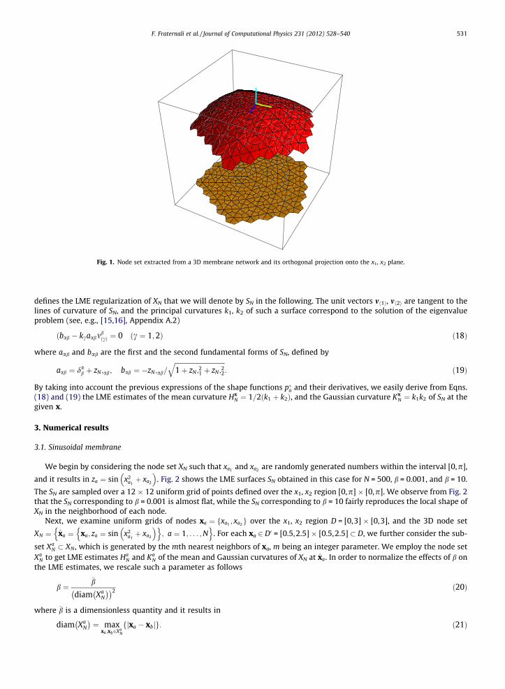
Fig. 1. Node set extracted from a 3D membrane network and its orthogonal projection onto the x1, x2 plane.


defines the LME regularization of XN that we will denote by SN in the following. The unit vectors mh1i, mh2i are tangent to thelines of curvature of SN, and the principal curvatures k1, k2 of such a surface correspond to the solution of the eigenvalueproblem (see, e.g., [15,16], Appendix A.2)

ðbab � kcaabmbðcÞ ¼ 0 ðc ¼ 1;2Þ ð18Þ

where aab and bab are the first and the second fundamental forms of SN, defined by

aab ¼ dab þ zN;ab; bab ¼ �zN;ab=

ffiffiffiffiffiffiffiffiffiffiffiffiffiffiffiffiffiffiffiffiffiffiffiffiffiffiffiffiffiffiffi1þ zN;

21 þ zN;

22

q: ð19Þ

By taking into account the previous expressions of the shape functions p�a and their derivatives, we easily derive from Eqns.(18) and (19) the LME estimates of the mean curvature Hx

N ¼ 1=2ðk1 þ k2Þ, and the Gaussian curvature KxN ¼ k1k2 of SN at the

given x.

3. Numerical results

3.1. Sinusoidal membrane

We begin by considering the node set XN such that xa1 and xa2 are randomly generated numbers within the interval [0,p],

and it results in za ¼ sin x2a1þ xa2

� �. Fig. 2 shows the LME surfaces SN obtained in this case for N = 500, b = 0.001, and b = 10.

The SN are sampled over a 12 � 12 uniform grid of points defined over the x1, x2 region [0,p] � [0,p]. We observe from Fig. 2that the SN corresponding to b = 0.001 is almost flat, while the SN corresponding to b = 10 fairly reproduces the local shape ofXN in the neighborhood of each node.

Next, we examine uniform grids of nodes xa ¼ fxa1 ; xa2g over the x1, x2 region D = [0,3] � [0,3], and the 3D node set

XN ¼ x̂a ¼ xa; za ¼ sin x2a1þ xa2

� �n o; a ¼ 1; . . . ;N

n o. For each xa 2 D0 = [0.5,2.5] � [0.5,2.5] D, we further consider the sub-

set XaN XN , which is generated by the mth nearest neighbors of xa, m being an integer parameter. We employ the node set

XaN to get LME estimates Ha

N and KaN of the mean and Gaussian curvatures of XN at x̂a. In order to normalize the effects of b on

the LME estimates, we rescale such a parameter as follows

b ¼�b

diam XaN

� �� 2 ð20Þ

where �b is a dimensionless quantity and it results in

diam XaN

� �¼ max

xa ;xb2XaN

fjxa � xbjg: ð21Þ

Fig. 2. LME approximations of scattered data extracted from the sinusoidal surface S : z = sin(x12 + x2) for two different values of b.

20 40 60 80 100 120 140β

0.005

0.010

0.015

0.020

0.025

0.030RMSD

RMSD KN

RMSD HN

0.035 0.040 0.045 0.050 0.055h

0.001

0.002

0.003

0.004

RMSD

RMSD KN

RMSD HN

Fig. 3. Root Mean Square Deviations (RMSD) of the LME approximations to the mean curvature H and the Gaussian curvature K of the sinusoidal surfacez ¼ sin x2

1 þ x2� �

over the x1, x2 domain [0.5, 2.5] � [0.5,2.5]. Left: RMSD as a function of �b, for m = 10 and h = 0.0303. Right: RMSD as a function of h, for m = 10and �b ¼ 150.


It is useful to compare HaN and Ka

N with the ‘exact’ counterparts Ha and Ka, which are easily computed through (18) and (19),by replacing zN with z ¼ sin x2

1 þ x2� �

. The accuracy of the nodal LME estimates HN ¼ HaN; a ¼ 1; . . . ;N0

� and

KN ¼ KaN; a ¼ 1; . . . ;N0

� can be inspected by examining the following Root Mean Square Deviations (RMSD)

RMSDðHNÞ ¼

ffiffiffiffiffiffiffiffiffiffiffiffiffiffiffiffiffiffiffiffiffiffiffiffiffiffiffiffiffiffiffiffiffiffiffiffiffiffiffiffiffiffiffiffiffiffiffiffiffiXN0a¼1

HaN � Ha� �2

� ,N0

vuut ;

RMSDðKNÞ ¼

ffiffiffiffiffiffiffiffiffiffiffiffiffiffiffiffiffiffiffiffiffiffiffiffiffiffiffiffiffiffiffiffiffiffiffiffiffiffiffiffiffiffiffiffiffiffiffiffiffiXN0a¼1

KaN � Ka� �2

� ,N0

vuut ð22Þ

for different values of �b and m. Here, N0 denotes the total number of nodes belonging to D0. We examine the following threedifferent mesh sizes: h = 0.0566 (N = 54 � 54); h = 0.0405 (N = 75 � 75); and h = 0.0303 (N = 100 � 100). Here and in the fol-lowing examples, we solve the nonlinear optimization problem (8) using recursive Newton–Raphson updates (9), up to thetermination condition jrkj < 10�6 diamðXa

NÞ. Fig. 3 illustrates how the quantities RMSD(HN) and RMSD(KN) vary with �b and hfor fixed m = 10, while Figs. 4–6 depict 2D and 3D density plots of the data sets HN and KN for several values of m, keeping�b ¼ 150, and h = 0.0303 fixed. The results shown in Figs. 4–6 point out that the LME estimates HN and KN exhibit uniformasymptotic convergence to the exact solutions H and K, respectively, for �b P 100;m P 9, and h 6 0.0303.

Fig. 4. 2D density plots of the LME approximations to the mean curvature H of the sinusoidal surface z ¼ sin x21 þ x2

� �over the x1, x2 domain

[0.5,2.5] � [0.5,2.5], for �b ¼ 150;h ¼ 0:0303, and different values of m (lower bound of the color bar: �4; upper bound: +4).


3.2. Spherical membrane

We examine, in the present and the following sections, a closed membrane network XN corresponding to the CGMDmodel of the red blood cell given in [2,3]. Such a model describes the system formed by the cytoskeleton spectrin network,the lipid bilayer and the transmembrane proteins of an actual RBC membrane, through a network of N (virtual) particlesembedded in a closed polyhedral surface showing M triangular facets. Each particle has sixfold coordination, with theexception of twelve ‘defects,’ which instead have fivefold coordination. The particles represent discrete areas of the RBCmembrane and their equilibrium distance r0 is set equal to the average length of the spectrin filaments (100 nm). Eachparticle has mass m and is connected to it’s nearest neighbors though linear springs of stiffness k, which are parameterizedsuch that the network of particles reproduces the membrane rigidity of a RBC. The bending rigidity is also accounted for

Fig. 5. 2D density plots of the LME approximations to the Gaussian curvature K of the sinusoidal surface z ¼ sin x21 þ x2


[0.5,2.5] � [0.5,2.5], for �b ¼ 150;h ¼ 0:0303, and different values of m (lower bound of the color bar: �0.56; upper bound: +0.56).


by introducing dihedral angle potential energy terms of angular stiffness D between adjacent triangles. The global surfacearea of the polyhedral membrane is kept constant using Lagrange multipliers, in order to mimic the relative incompress-ibility of the lipid bilayer of a normal RBC. The model under consideration is also able to keep the volume enveloped bythe polyhedral membrane constant, with the aim to resemble the typical behaviour of a RBC in normal conditions. Thedynamics of the RBC model can be obtained by integrating the Newton equations of motion of each virtual particle usinga standard MD code. We used DL POLY 2.20 ([17]), and employed the Nosé-Hoover thermostat; 6 � 106 steps with time-step Dt = 2.07 � 10�5 t0, where t0 ¼

ffiffiffiffiffiffiffiffiffiffim=k

p; N ¼ 5762 particles; m = 5.82625 � 10�20 kg; k = 8.3 lN/m; D = 130 � 10�20 J;

constant absolute temperature T = 309 K; constant surface area A ¼ 4:986� 107 nm2; and constant volumeV ¼ 3:311� 1010 nm3. Such parameter settings allow the LME regularization to approximate a spherical surface S withradius �r ¼ 1992 nm [2].


The theoretical average surface S clearly has uniform principal curvatures k1 ¼ k2 ¼ H ¼ �1=�r ¼ �5:019� 10�4 nm�1 (theminus sign follows from the outward orientation of the normal vector), and Gaussian curvatureK = k1k2 = 25.19 � 10�8 nm�2. Nodal LME estimates HN ¼ Ha

N; a ¼ 1; . . . ;N�

and KN ¼ KaN; a ¼ 1; . . . ;N

� of the mean and

Gaussian curvatures of the network can be obtained by introducing different local frames fx̂a; x1; x2; zg at each differentnode x̂a, with x1, x2 and z tangent to the local parallel, meridian, and radial lines, respectively. Table 1 shows the mean valuesand the standard deviations of the data sets HN and KN defined as follows

Fig. 6.[0.5,2.5

Table 1Mean aand diff

HN �sd(HN

KN �sd(KN

HN ¼ 1=NXN

a¼1

HaN; sdðHNÞ ¼

ffiffiffiffiffiffiffiffiffiffiffiffiffiffiffiffiffiffiffiffiffiffiffiffiffiffiffiffiffiffiffiffiffiffiffiffiffiffiffiffiffiffiffiffiffiffiffiffiffiffiffiffiffiffiffiffiffiffiffiffiffiXN

a¼1

HaN � HN

� �2� ,ðN � 1Þ

vuut ð23Þ

KN ¼ 1=NXN

a¼1

KaN; sdðKNÞ ¼

ffiffiffiffiffiffiffiffiffiffiffiffiffiffiffiffiffiffiffiffiffiffiffiffiffiffiffiffiffiffiffiffiffiffiffiffiffiffiffiffiffiffiffiffiffiffiffiffiffiffiffiffiffiffiffiffiffiffiffiffiffiXN

a¼1

KaN � KN

� �2� ,ðN � 1Þ

vuut ð24Þ

for �b ¼ 100 and different values of m. The results in Table 1 highlight a good agreement between LSM estimates and exactsolutions for m P 10. It has to be considered that the MD model doesn’t reach a perfectly (average) spherical shape at equi-librium, due to the presence of the fivefold defects.

3.3. Principal curvatures of the RBC membrane

We analyze in the present section a slight different formulation of the RBC model given in [2,3], which differs from thatdiscussed in the previous section only in terms of the volume constraint. Here, we set the volume enveloped by the RBCmembrane equal to 0.65 times the volume of the sphere analyzed in the previous example, allowing the current model toassume the typical biconcave shape of a normal RBC [3].The surface area of the RBC membrane is again set to4.986 � 107 nm2, as in the previous case. We compute nodal LME estimates HN ¼ Ha

N; a ¼ 1; . . . ;N�

andKN ¼ Ka

N; a ¼ 1; . . . ;N�

of the mean and Gaussian curvatures of a real RBC membrane by processing the rolling mean shapesXN of the CGMD model up to different simulation times t. Let n denote the weighted unit normal to the current vertex x̂a of

3D density plots of the LME approximations to the mean and the Gaussian curvatures of the sinusoidal surface z ¼ sin x21 þ x2


] � [0.5,2.5], for �b ¼ 150;h ¼ 0:0303, and m = 12.

nd standard deviation of the data sets HN and KN for a spherical membrane network with N = 5762 nodes and radius r = 1992 nm, considering �b ¼ 100erent values of m. Exact solution: H = �5.019 � 10�5 Å�1, K = 25.19 � 10�10 Å�2.

m = 5 m = 7 m = 9 m = 10 m = 12

105 Å�1 39.0626 �7.1062 �5.1293 �5.0443 �5.0311

) � 105 Å�1 2.8047 0.1467 0.0296 0.0271 0.0238

1010 Å�2 1540.19 50.488 26.3077 25.4453 25.3118

) � 1010 Å�2 234.04 2.1551 0.3152 0.2840 0.2473


the triangulation associated with XN, assuming the triangle areas as the weights [18]. In the present case, we define the localx1 axis as the direction of the edge attached to x̂a that has the minimum deviation from the parallel drawn on an ideal spherepassing through the same point. In addition, we define x2 by means of the vector product of the unit vectors in the directionsof n and x1, and z via the vector product of the unit vectors in the directions of x1 and x2. A graphical representation of thelocal parameterization introduced for the analyzed model of the RBC membrane is provided in Fig. 7.

Fig. 8 shows the dependence of the LME estimates HN and KtotN ¼ KNA on �b, for t = 75.5 t0 and m = 10. It is worth noting that

KtotN represents an estimate of the total curvature Ktot ¼

RSN

K dA of the RBC model. Due to the ‘Gauss-Bonet theorem’ such aquantity only depends on the genus of SN and should be equal to 4p, as in the case of a sphere [15]. One observes from Fig. 8slight oscillations of HN and Ktot

N with �b; KtotN =4 � 3:00 for �b < 100; and Ktot

N =4 � 3:14 for �b ¼ 125. 3D density plots of the datasets HN and KN are given in Figs. 9 and 10, considering �b ¼ 125;m ¼ 10, and different simulation times t. The results shown inFigs. 9 and 10 indicate that the LME regularizations of the average CGMD configurations smoothly describe the geometry of anormal RBC membrane. The LME regularization is indeed able to reproduce the biconcave shape of such a membrane (con-sider that the hidden bottom edges of the surfaces shown in Figs. 9 and 10 are nearly specular with respect to the top ones),furnishing positive (red) and negative (blue) mean curvatures in correspondence with concave and convex portions, respec-tively (cf. Fig. 9), and negative (blue) Gaussian curvatures over saddle-shaped regions (cf. Fig. 10). One observes perturba-tions in the mean and Gaussian curvature maps in correspondence with the fivefold defects of the membranetriangulation during the initial phase of the MD simulation. The MD simulation and the LME regularization are however ableto smooth out the local noise produced by such perturbations, as the simulation time progressively increases.

3.4. Estimation of the bending rigidity of membrane networks from MD simulations

Let us consider now a triangulated membrane network endowed with the following dihedral angle energy

Fig. 7.(For int

Fig. 8.

Edihedral ¼ DX

M;M0 2 CM

neighbors

ð1� cos dMM0 Þ ¼ D2

XM;M0 2 CM

neighbors

jnM � nM0 j2ð25Þ

3D map of the local bases fx̂a; x1; x2; zg introduced at selected nodes of a triangulated model of the RBC membrane (x1: yellow, x2: blue, z: cyan).erpretation of the references to colour in this figure legend, the reader is referred to the web version of this article.)

50 75 100 125β2.0

3.0

4.0

5.0

6.0H , K

KNtot4

HN

LME estimates jbHN j ¼ jHN j � 105 Å�1

and KtotN for a CGMD model of the RBC membrane [2,3], considering different values of �b;m ¼ 10, and t = 75.5 t0.

Fig. 9. 3D density plots of the LME approximations HN to the mean curvature H of of a CGMD model of the RBC membrane [2,3] at different simulation timest, for �b ¼ 125 and m = 10 (bHN ¼ HN � 105 Å

�1; lower bound of the color bar: �11.5 � 10�5 Å�1; upper bound: +2.5 � 10�5 Å�1).


where CM denotes the set of all triangles forming the network; dMM0 is the dihedral angle between the triangles M and M0; nM isthe unit normal to the triangle M; and the summation runs over all the pairs M;M0 2 CM which share a common side. Accord-ing to [7,8], the limiting bending energy of such a network is a Helfrich-type bending energy [19] of the form

Ebend ¼ jH

2

ZSN

ðð2HÞ2 � 2KÞdS ð26Þ

where jH is the bending rigidity, and it results jH ¼ffiffiffi3p

D=3 for a sphere, and jH ¼ffiffiffi3p

D=2 for a cylinder [8]. (Note that in[7,8] the symbol H is used to denote twice the mean curvature of the network.)

The LME prediction of the principal curvatures of the network allows us to estimate the limiting bending energy (26). As amatter of fact, the computing of the mean curvatures HN ¼ Ha

N; a ¼ 1; . . . ;N�

of the current configuration leads us to approx-imate (26) as follows

EbendN ¼ jH

2

XN

a¼1

2HaN

� �2AaN

!� 8p

" #ð27Þ

Fig. 10. 3D density plots of the LME approximations KN to the Gaussian curvature K of a CGMD model of the RBC membrane [2,3] at different simulationtimes t, for �b ¼ 125 and m = 10 (lower bound of the color bar: �2 � 10�9 Å�2; upper bound: +7 � 10�9 Å�2).


where AaN is the surface area of the a-th element of a dual tessellation of the network, which we assume is formed by poly-

gons joining the midpoints of the network edges with the triangle barycenters (barycentric dual mesh). Eq. (27) can be em-ployed to estimate the Cauchy–Born contribution [20,21] to the isothermal bending rigidity, here denoted by j0

H . The latter

consists of the configurational average of the instantaneous bending rigidities of the fluctuating network. On matching EbendN

to Edihedral, we identify the instantaneous bending rigidity with the ratio Edihedral EbendN

� ��jH¼1

and compute j0

H through

j0H ¼

Edihedral

EbendN

� ��jH¼1

* +ð28Þ

where h � i denotes the configurational average symbol.For the sake of example, let us reconsider now the MD model of the RBC membrane examined in the previous section.

Fig. 11 shows the time history that we obtained for the bending rigidity j0H of such a model, on computing the rolling

3 D 3

3 D 2

numeric

20 40 60 80 100t t0

70

80

90

100

110

120

130

Fig. 11. LME estimates of the Born contribution to the bending rigidity of the RBC membrane model presented in Section 3.3, at different times of a MDsimulation.


averages of the instantaneous bending rigidities during a MD simulation (cf. Section 3.3). It is seen from Fig. 11 that the valueof j0

H slightly fluctuates during the simulation, featuring oscillations with progressively smaller amplitude as the computa-tional time t increases. We estimated a limiting value of j0

H approximatively equal to 79 J, for t > 100 t0. Such a value is justslightly greater than that predicted in [8] for the sphere

ffiffiffi3p

D=3 ¼ 75:06 J� �

, which is not surprising, since the biconcave(mean) shape of the RBC model under consideration has the same genus of the sphere.

4. Concluding remarks

We have presented and numerically tested a meshfree approach to the curvature and bending rigidity estimation ofmembrane networks, through a suitable extension of the LME method formulated in [1]. The results of Sections 3.1 and3.2 demonstrate the convergence properties of the LME curvature estimates, both for a rectangular geometry (fixed{x1,x2,z} axes), and for a spherical membrane. On the other hand, the results presented in Sections 3.3 and 3.4, emphasizethe ability of the LME approach in tracking the local curvatures and the bending rigidity of the RBC model presented in[2]. Concerning the parameter estimation, we have found that the limitations �b P 100 and m P 10 generally ensure stablecurvature predictions. In particular, for m P 10 we found that100 is approximately the smallest value of �b that guaranteesasymptotic convergence of LME curvature predictions for the examined examples. The value of �b rules the degree of localityof LME approximations, which reduce to piecewise affine shape functions supported by a Delaunay triangulation for �b!1[1,11].

In closing, we suggest some directions for relevant extensions of the present work. We intend to apply the LME regular-ization algorithm to predict the entire set of the isothermal membrane and bending rigidities of fluctuating biomembranesmodeled through MD simulations, with special reference to the RBC membrane. We plan to combine the LME regularizationof the RBC model proposed in [2], with the elastic moduli estimation procedures given in [7,8,21]. Another application of theLME procedure presented in this work is to mesure the curvature of lipid bilayers as modelled with MD simulations. Lipidbilayers are generally flat, however several different protein-driven processes will result in the membrane curvature that isrequired for various cell processes (i.e. fusion). One mechanism is caused by protein domains inserting shallowly into one ofthe lipid leaflets, which push the neighboring lipid head groups away and therefore causing local spontaneous curvature. Weare currently conducting coarse-grain MD simulations that model the interactions between different varieties of these pro-tein domains and lipid bilayers. The LME procedure will allow us to quantify the amount of curvature that results from theseinteractions.

Acknowledgements

F. F. wishes to acknowledge the great support received by Ada Amendola (Department of Civil Engineering, University ofSalerno), Bo Li (Graduate Aerospace Laboratories, California Institute of Technology), and Franca Fraternali (Randall Divisionof Cell and Molecular Biophysics, King’s College London) during the course of the present work.

References

[1] M. Arrojo, M. Ortiz, Local maximum-entropy approximation schemes: a seamless bridge between finite elements and meshfree methods, Int. J. Num.Meth. Eng. 65 (2006) 2167–2202.

[2] G. Marcelli, H.K. Parker, P. Winlove, Thermal fluctuations of red blood cell membrane via a constant-area particle-dynamics model, Biophys. J. 89(2005) 2473–2480.


[3] J.P. Hale, G. Marcelli, K.H. Parker, C.P. Winlowe, G.P. Petrov, Red blood cell thermal fluctuations: comparison between experiment and moleculardynamics simulations, Soft Matt. 5 (2009) 3603–3606.

[4] H.J. Risselada, S.J. Marrink, Curvature effects on lipid packing and dynamics in liposomes revealed by coarse grained molecular dynamics simulations,Phys. Chem. Chem. Phys. 11 (2009) 2056–2067.

[5] S. Martens, H.T. McMahon, Mechanisms of membrane fusion: disparate players and common principles, Nature Rev. 9 (2008) 543–556.[6] H.T. McMahon, J.L. Gallop, Membrane curvature and mechanisms of dynamic cell membrane remodelling, Nature 438 (2005) 590–596.[7] H.S. Seung, D.R. Nelson, Defects in Flexible Membranes with Crystalline Order, Phys. Rev. A 38 (1988) 1005–1018.[8] G. Gompper, D.M. Kroll, Random Surface Discretization and the Renormalization of the Bending Rigidity, J. Phys. I France 6 (1996) 1305–1320.[9] Q. Du, C. Liu, X. Wang, Simulating the deformation of vescicle membranes under elastic bending energy in three dimensions, J. Comput. Phys. 212

(2006) 757–777.[10] M. Dao, J. Li, S. Suresh, Molecularly based analysis of deformation of spectrin network and human erythrocyte, Mat. Sci. Eng. C 26 (2006) 1232–1244.[11] C.J. Cyron, M. Arrojo, M. Ortiz, Smooth, second-order, non-negative meshfree approximants selected by maximum entropy, Int. J. Num. Meth. Eng. 79

(2009) 1605–1632.[12] B. Li, F. Habbal, M. Ortiz, Optimal transportation meshfree approximation schemes for fluid and plastic flows, Int. J. Num. Meth. Eng. (2010).

doi:10.1002/nme.2869.[13] E.T. Jaines, Information theory and statistical mechanics, Phys. Rev. 106 (1957) 620–630.[14] V.T. Rajan, Optimality of the Delunay triangulation in Rd, Discrete Comput. Geom. 12 (2) (1994) 189–202.[15] J.J. Stoker, Differential Geometry, Wiley, New York, 1969.[16] P.M. Naghdi, The Theory of Shells and Plates, in: C. Trusdell (Ed.), S. Flügge’s Handbuch der Physik, Vol. VIa/2, Springer Verlag, Berlin, Heidelberg, New

York, 1972, pp. 425–640.[17] W. Smith, T.R. Forester, The DL_POLY_2 molecular simulation package. (1999) <http://www.cse.clrc.ac.uk/msi/software/DL_POLY>.[18] G. Taubin, Estimating the tensor of curvature of a surface from a polyhedral approximation, in: Proceedings of the 5th International Conference on

Computer Vision (ICCV’95). Cambridge, MA: MIT. (1995) 902-907.[19] H.J. Deuling, W. Helfrich, Red blood cell shapes as explained on the basis of curvature elasticity, Biophys J. 16 (8) (1976) 861–868.[20] J.L. Ericksen, On the Cauchy–Born Rule, Math. Mech. Solids 13 (2008) 199–220.[21] Z. Zhou, B. Joós, Stability criteria for homogeneously stressed materials and the calculation of elastic constants, Phys. Rev. B 54 (6) (1996) 3841–3850.

http://dx.doi.org/10.1002/nme.2869

http://www.cse.clrc.ac.uk/msi/software/DL_POLY

Journal of Computational Physics · a Department of Civil Engineering, University of Salerno, 84084...

Documents

Transcript of Journal of Computational Physics · a Department of Civil Engineering, University of Salerno, 84084...