CAN PARAMETRIC STATISTICAL METHODS BE TRUSTEDFOR FMRI BASED GROUP STUDIES?

Anders Eklund a,b,c, Thomas Nichols d, Hans Knutsson a,c

aDivision of Medical Informatics, Department of Biomedical Engineering,Linkoping University, Linkoping, Sweden

bDivision of Statistics and Machine Learning, Department of Computer and Information Science,Linkoping University, Linkoping, Sweden

cCenter for Medical Image Science and Visualization (CMIV),Linkoping University, Linkoping, Sweden

dDepartment of Statistics, University of Warwick, Coventry, United Kingdom

ABSTRACTThe most widely used task fMRI analyses use paramet-

ric methods that depend on a variety of assumptions. Whileindividual aspects of these fMRI models have been evalu-ated, they have not been evaluated in a comprehensive man-ner with empirical data. In this work, a total of 2 millionrandom task fMRI group analyses have been performed usingresting state fMRI data, to compute empirical familywise er-ror rates for the software packages SPM, FSL and AFNI, aswell as a standard non-parametric permutation method. Whilethere is some variation, for a nominal familywise error rate of5% the parametric statistical methods are shown to be conser-vative for voxel-wise inference and invalid for cluster-wiseinference; in particular, cluster size inference with a clus-ter defining threshold of p = 0.01 generates familywise errorrates up to 60%. We conduct a number of follow up anal-yses and investigations that suggest the cause of the invalidcluster inferences is spatial auto correlation functions that donot follow the assumed Gaussian shape. By comparison, thenon-parametric permutation test, which is based on a smallnumber of assumptions, is found to produce valid results forvoxel as well as cluster wise inference. Using real task data,we compare the results between one parametric method andthe permutation test, and find stark differences in the conclu-sions drawn between the two using cluster inference. Thesefindings speak to the need of validating the statistical methodsbeing used in the neuroimaging field.

1. INTRODUCTION

Functional magnetic resonance imaging (fMRI) [1, 2] hassince its beginning some 20 years ago been a popular tool forincreasing the knowledge about the human brain, with some28,000 published papers according to PubMed (fMRI in the

title or abstract). The first fMRI experiments consisted ofsimple motor tasks, while more recent examples involve rest-ing state fMRI to study (dynamic) brain connectivity [3, 4].Despite the popularity of fMRI as a tool for studying brainfunction, the statistical methods used have rarely been vali-dated using real data, likely due to the high cost of fMRI datacollection. Validations have instead mainly been performedusing simulated data [5], but it is obviously very hard tosimulate the complex spatiotemporal noise that arises from aliving human subject in an MR scanner.

Through the introduction of international data sharing ini-tiatives in the neuroimaging field [6, 7, 8, 9, 10, 11, 12], it hasbecome possible to evaluate the statistical methods using realdata. Scarpazza et al. [13] for example used freely availableanatomical images from 396 healthy controls [6] to investi-gate the validity of parametric statistical methods for voxelbased morphometry [14], when comparing a single subjectto a group. Silver et al. [15] instead used image and genotypedata from 181 subjects in the Alzheimer’s disease neuroimag-ing initiative (ADNI) [10, 11]. The data were used to evaluatestatistical methods common in imaging genetics, where thegoal is to find genes that can explain variation in brain struc-ture or function. Another example of the use of open datais our previous work [16], where we investigated the valid-ity of the SPM software for single subject fMRI analysis. Atotal of 1484 resting state fMRI data sets from the 1000 func-tional connectomes project [6] were used as null data, to testhow likely it is to find significant brain activity when a sub-ject has not performed any specific task in the MR scanner.The main conclusion was that the noise model in SPM is toosimple, yielding a high degree of false positives (up to 70%incidence of any false positives, compared to the expected 5%under familywise error control). It was, however, not clear ifthese problems would propagate to group studies, where inter-

1

arX

iv:1

511.

0186

3v1

[st

at.A

P] 5

Nov

201

5

subject variability in a per-subject response is less complexthan intrasubject time series data. Another unanswered ques-tion was the statistical validity of other fMRI software pack-ages. Here, we therefore present a statistical evaluation of thethree most common fMRI software packages (SPM [17, 18],FSL [19], AFNI [20]) for group inference. Specifically, weevaluate the packages in their entirety, submitting the null datato recommended suite of preprocessing steps integrated intoeach package.

The main idea of this study is the same for our previousone [16]; to analyze null data and simply count the numberanalyses that give rise to any false positives. Since two groupsof subjects are randomly drawn from a group of healthy con-trols, the null hypothesis of no group difference in brain ac-tivation is true. By performing many random group compar-isons, using only healthy controls of similar age, it is possibleto compute the empirical false positive rate of a two samplet-test. A similar approach has previously been used to in-vestigate the validity of parametric statistics for voxel basedmorphometry [14, 21]. Using resting state fMRI data, whichshould not contain specific forms of brain activity, it is alsopossible to compute the empirical false positive rate of a onesample t-test (group activation).

Briefly, our results show that the parametric statisticalmethods used in the three most common fMRI softwarepackages are conservative for voxel-wise inference with fam-ilywise error control, where each voxel in a volume is inde-pendently tested for significance. However, the parametricmethods can give a very high degree of false positives (upto 60%, compared to the nominal 5%) for cluster-wise infer-ence [22, 23, 24], where groups of neighboring voxels aretested simultaneously (to increase the statistical power). Bycomparison, the non-parametric permutation test [25, 26] isfound to produce valid results for both voxel- and cluster-wiseinference.

2. RESULTS

A total of 1,920,000 random group analyses were performedto compute the empirical false positive rates of SPM, FSLand AFNI (1,000 random analyses repeated for 128 parametercombinations, three thresholding approaches and five func-tions in the three softwares). The tested parameter combi-nations, given in Table 1, are common in the fMRI field ac-cording to a recent review [27]. The following five softwaretools were tested; SPM OLS, FSL OLS, FSL FLAME1, AFNIOLS (3dttest++) and AFNI 3dMEMA. The OLS (ordinaryleast squares) functions only use the beta estimates from eachsubject in the group analysis, while FLAME1 in FSL and3dMEMA in AFNI also consider the variance of the beta esti-mates. To compare the parametric statistical methods used bySPM, FSL and AFNI to a non-parametric method, all analy-ses were also performed using a permutation test [25, 26, 28].

Resting state fMRI data from 396 healthy controls, down-

loaded from the 1000 functional connectomes project [6],were used for all of the analyses. Resting state data shouldnot contain systematic changes in brain activity, but our pre-vious work [16] showed that the used (pretended) activityparadigm can have a large impact on the degree of false pos-itives. Several different activity paradigms were thereforeused; two block based (B1, B2) and two event related (E1,E2), see Table 2.

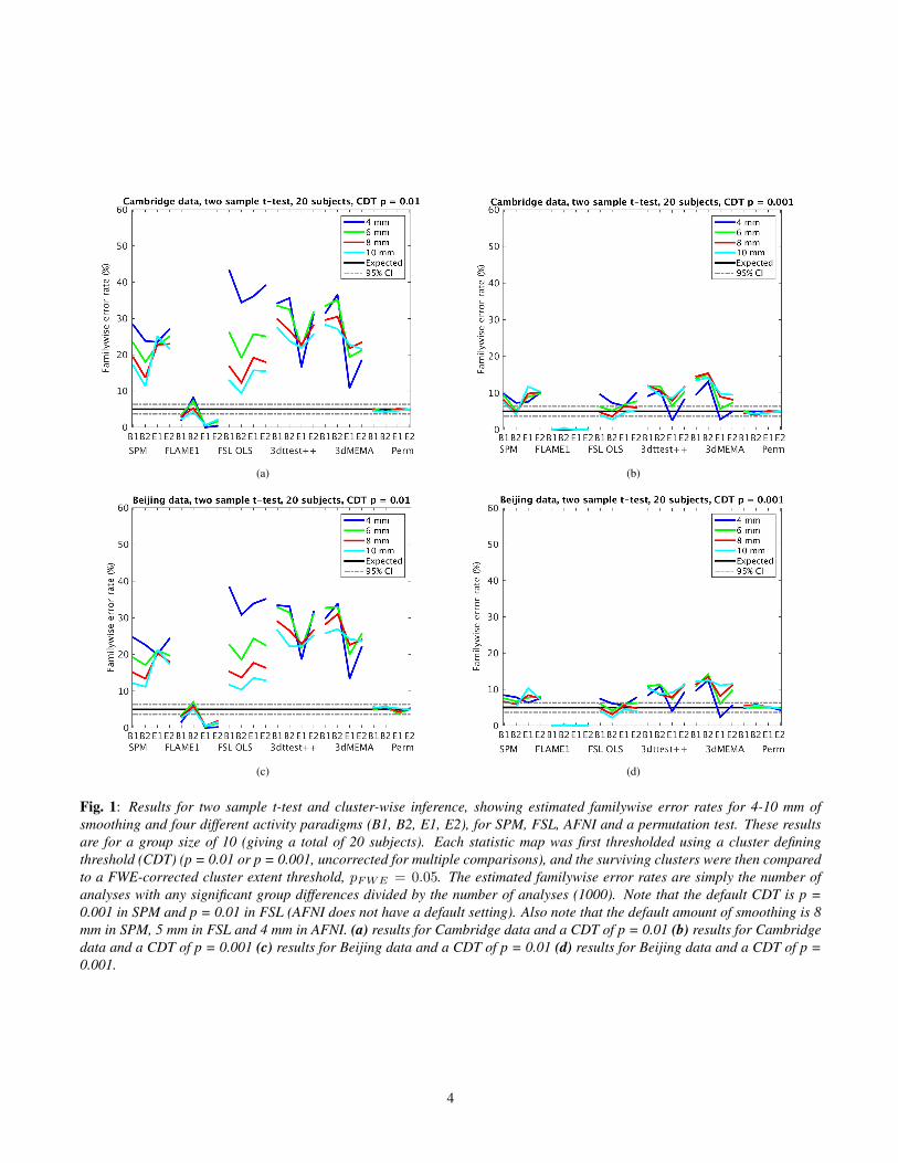
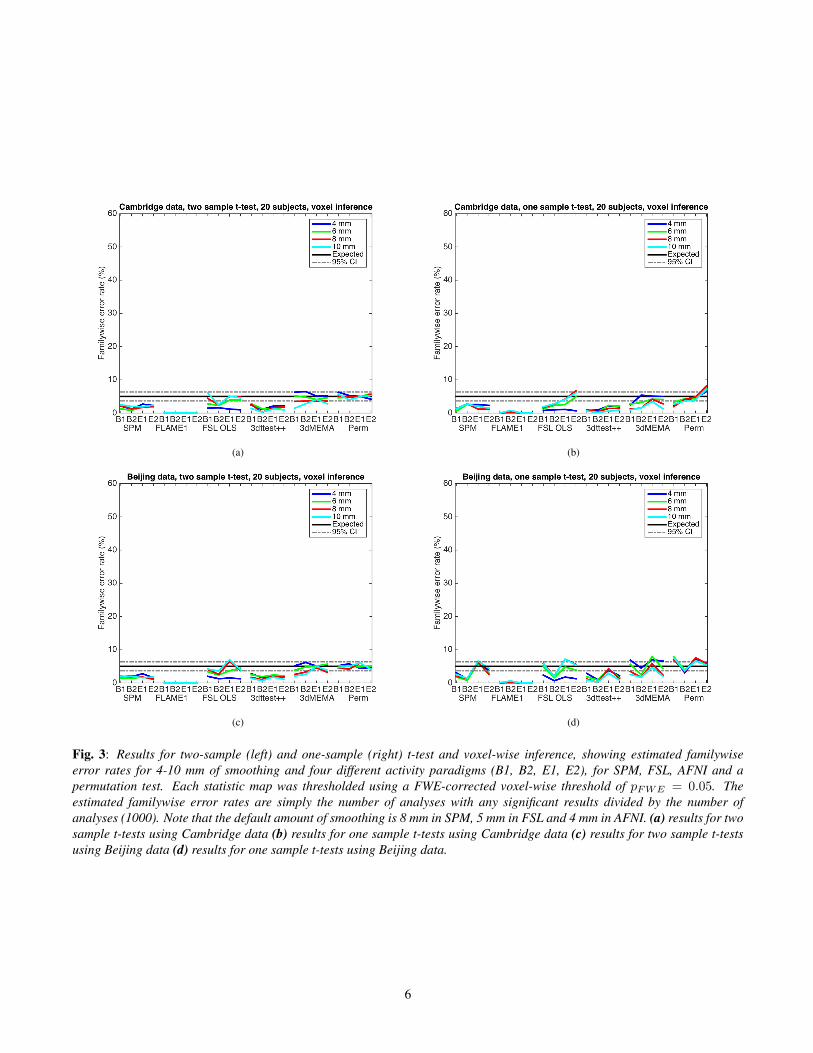
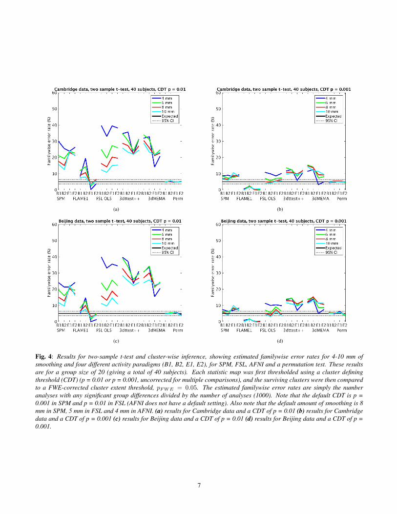
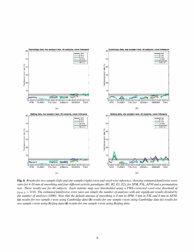
Figures 1 - 3 present the main findings of the study, show-ing cluster-wise (Figure 1, two-sample t-test; Figure 2, one-sample t-test) and voxel-wise (Figure 3) results for a totalsample size of 20 (Figures 4 - 6 show corresponding resultsfor a total sample size of 40). In broad summary, parametricsoftware’s familywise error (FWE) rates for cluster-wise in-ference far exceed their nominal 5% level, while parametricvoxel-wise inferences are valid but often conservative, oftenfalling below 5%. Permutation false positives are controlledat a nominal 5% except for cluster-wise inference with a onesample t-test, mainly with the Beijing data with designs B1and E1. The impact of cluster defining threshold (CDT) wasappreciable for the parametric methods, with CDT p = 0.001having much better FWE control than CDT p = 0.01. Amongthe parametric software packages, FSL’s FLAME1 cluster-wise inference stood out as having much lower FWE, oftenbeing valid (under 5%). But with cluster-wise CDT p = 0.001,and voxel-wise inference, FLAME1 was often very conserva-tive.

2

Table 1: Parameters tested for the different fMRI software packages, giving a total of 128 parameter combinations and 3thresholding approaches. One thousand group analyses were performed for each parameter combination.

Parameter Values usedfMRI data Beijing (198 subjects), Cambridge (198 subjects)

Activity paradigm Block (B1, B2), event (E1, E2)Smoothing 4, 6, 8, 10 mm FWHM

Analysis type One sample t-test (group activation), two sample t-test (group difference)Number of subjects 20, 40

Inference level Voxel, clusterCluster defining threshold p = 0.01 (z = 2.3), p = 0.001 (z = 3.1)

Table 2: Length of activity and rest periods for the used (pretended) activity paradigms, R stands for randomized. Number ofperiods

Paradigm Activity duration (s) Rest duration (s)B1 10 10B2 30 30E1 2 6E2 1-4 (R) 3-6 (R)

3

(a) (b)

(c) (d)

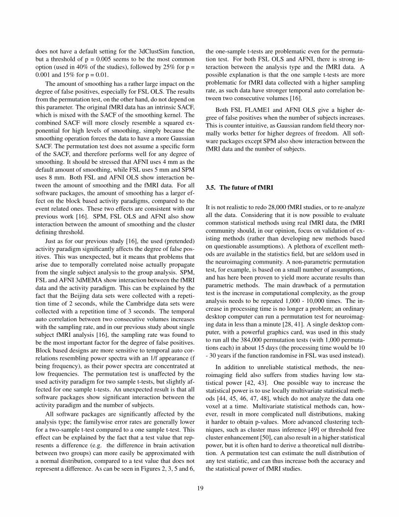
Fig. 1: Results for two sample t-test and cluster-wise inference, showing estimated familywise error rates for 4-10 mm ofsmoothing and four different activity paradigms (B1, B2, E1, E2), for SPM, FSL, AFNI and a permutation test. These resultsare for a group size of 10 (giving a total of 20 subjects). Each statistic map was first thresholded using a cluster definingthreshold (CDT) (p = 0.01 or p = 0.001, uncorrected for multiple comparisons), and the surviving clusters were then comparedto a FWE-corrected cluster extent threshold, pFWE = 0.05. The estimated familywise error rates are simply the number ofanalyses with any significant group differences divided by the number of analyses (1000). Note that the default CDT is p =0.001 in SPM and p = 0.01 in FSL (AFNI does not have a default setting). Also note that the default amount of smoothing is 8mm in SPM, 5 mm in FSL and 4 mm in AFNI. (a) results for Cambridge data and a CDT of p = 0.01 (b) results for Cambridgedata and a CDT of p = 0.001 (c) results for Beijing data and a CDT of p = 0.01 (d) results for Beijing data and a CDT of p =0.001.

4

(a) (b)

(c) (d)

Fig. 2: Results for one sample t-test and cluster-wise inference, showing estimated familywise error rates for 4-10 mm ofsmoothing and four different activity paradigms (B1, B2, E1, E2), for SPM, FSL, AFNI and a permutation test. These resultsare for a group size of 20. Each statistic map was first thresholded using a cluster defining threshold (CDT) (p = 0.01 or p= 0.001, uncorrected for multiple comparisons), and the surviving clusters were then compared to a FWE-corrected clusterextent threshold, pFWE = 0.05. The estimated familywise error rates are simply the number of analyses with any significantgroup activations divided by the number of analyses (1000). Note that the default CDT is p = 0.001 in SPM and p = 0.01 inFSL (AFNI does not have a default setting). Also note that the default amount of smoothing is 8 mm in SPM, 5 mm in FSL and4 mm in AFNI. (a) results for Cambridge data and a CDT of p = 0.01 (b) results for Cambridge data and a CDT of p = 0.001(c) results for Beijing data and a CDT of p = 0.01 (d) results for Beijing data and a CDT of p = 0.001.

5

(a) (b)

(c) (d)

Fig. 3: Results for two-sample (left) and one-sample (right) t-test and voxel-wise inference, showing estimated familywiseerror rates for 4-10 mm of smoothing and four different activity paradigms (B1, B2, E1, E2), for SPM, FSL, AFNI and apermutation test. Each statistic map was thresholded using a FWE-corrected voxel-wise threshold of pFWE = 0.05. Theestimated familywise error rates are simply the number of analyses with any significant results divided by the number ofanalyses (1000). Note that the default amount of smoothing is 8 mm in SPM, 5 mm in FSL and 4 mm in AFNI. (a) results for twosample t-tests using Cambridge data (b) results for one sample t-tests using Cambridge data (c) results for two sample t-testsusing Beijing data (d) results for one sample t-tests using Beijing data.

6

(a) (b)

(c) (d)

Fig. 4: Results for two-sample t-test and cluster-wise inference, showing estimated familywise error rates for 4-10 mm ofsmoothing and four different activity paradigms (B1, B2, E1, E2), for SPM, FSL, AFNI and a permutation test. These resultsare for a group size of 20 (giving a total of 40 subjects). Each statistic map was first thresholded using a cluster definingthreshold (CDT) (p = 0.01 or p = 0.001, uncorrected for multiple comparisons), and the surviving clusters were then comparedto a FWE-corrected cluster extent threshold, pFWE = 0.05. The estimated familywise error rates are simply the numberanalyses with any significant group differences divided by the number of analyses (1000). Note that the default CDT is p =0.001 in SPM and p = 0.01 in FSL (AFNI does not have a default setting). Also note that the default amount of smoothing is 8mm in SPM, 5 mm in FSL and 4 mm in AFNI. (a) results for Cambridge data and a CDT of p = 0.01 (b) results for Cambridgedata and a CDT of p = 0.001 (c) results for Beijing data and a CDT of p = 0.01 (d) results for Beijing data and a CDT of p =0.001.

7

(a) (b)

(c) (d)

Fig. 5: Results for one-sample t-test and cluster-wise inference, showing estimated familywise error rates for 4-10 mm ofsmoothing and four different activity paradigms (B1, B2, E1, E2), for SPM, FSL, AFNI and a permutation test. These resultsare for a group size of 40. Each statistic map was first thresholded using a cluster defining threshold (CDT) (p = 0.01 or p= 0.001, uncorrected for multiple comparisons), and the surviving clusters were then compared to a FWE-corrected clusterextent threshold, pFWE = 0.05. The estimated familywise error rates are simply the number of analyses with significant groupactivations divided by the number of analyses (1000). Note that the default CDT is p = 0.001 in SPM and p = 0.01 in FSL(AFNI does not have a default setting). Also note that the default amount of smoothing is 8 mm in SPM, 5 mm in FSL and 4mm in AFNI. (a) results for Cambridge data and a CDT of p = 0.01 (b) results for Cambridge data and a CDT of p = 0.001 (c)results for Beijing data and a CDT of p = 0.01 (d) results for Beijing data and a CDT of p = 0.001.

8

(a) (b)

(c) (d)

Fig. 6: Results for two-sample (left) and one-sample (right) t-test and voxel-wise inference, showing estimated familywise errorrates for 4-10 mm of smoothing and four different activity paradigms (B1, B2, E1, E2), for SPM, FSL, AFNI and a permutationtest. These results are for 40 subjects. Each statistic map was thresholded using a FWE-corrected voxel-wise threshold ofpFWE = 0.05. The estimated familywise error rates are simply the number of analyses with any significant results divided bythe number of analyses (1000). Note that the default amount of smoothing is 8 mm in SPM, 5 mm in FSL and 4 mm in AFNI.(a) results for two sample t-tests using Cambridge data (b) results for one sample t-tests using Cambridge data (c) results fortwo sample t-tests using Beijing data (d) results for one sample t-tests using Beijing data.

9

2.1. What about other common cluster thresholding ap-proaches?

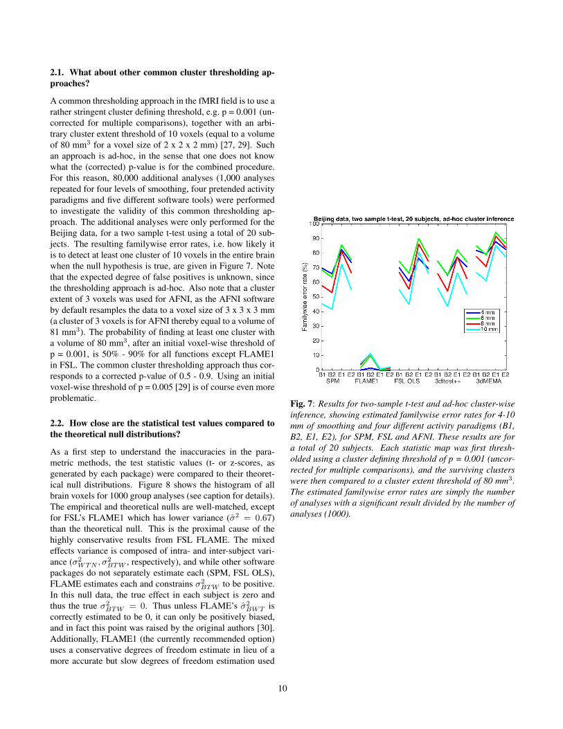
A common thresholding approach in the fMRI field is to use arather stringent cluster defining threshold, e.g. p = 0.001 (un-corrected for multiple comparisons), together with an arbi-trary cluster extent threshold of 10 voxels (equal to a volumeof 80 mm3 for a voxel size of 2 x 2 x 2 mm) [27, 29]. Suchan approach is ad-hoc, in the sense that one does not knowwhat the (corrected) p-value is for the combined procedure.For this reason, 80,000 additional analyses (1,000 analysesrepeated for four levels of smoothing, four pretended activityparadigms and five different software tools) were performedto investigate the validity of this common thresholding ap-proach. The additional analyses were only performed for theBeijing data, for a two sample t-test using a total of 20 sub-jects. The resulting familywise error rates, i.e. how likely itis to detect at least one cluster of 10 voxels in the entire brainwhen the null hypothesis is true, are given in Figure 7. Notethat the expected degree of false positives is unknown, sincethe thresholding approach is ad-hoc. Also note that a clusterextent of 3 voxels was used for AFNI, as the AFNI softwareby default resamples the data to a voxel size of 3 x 3 x 3 mm(a cluster of 3 voxels is for AFNI thereby equal to a volume of81 mm3). The probability of finding at least one cluster witha volume of 80 mm3, after an initial voxel-wise threshold ofp = 0.001, is 50% - 90% for all functions except FLAME1in FSL. The common cluster thresholding approach thus cor-responds to a corrected p-value of 0.5 - 0.9. Using an initialvoxel-wise threshold of p = 0.005 [29] is of course even moreproblematic.

2.2. How close are the statistical test values compared tothe theoretical null distributions?

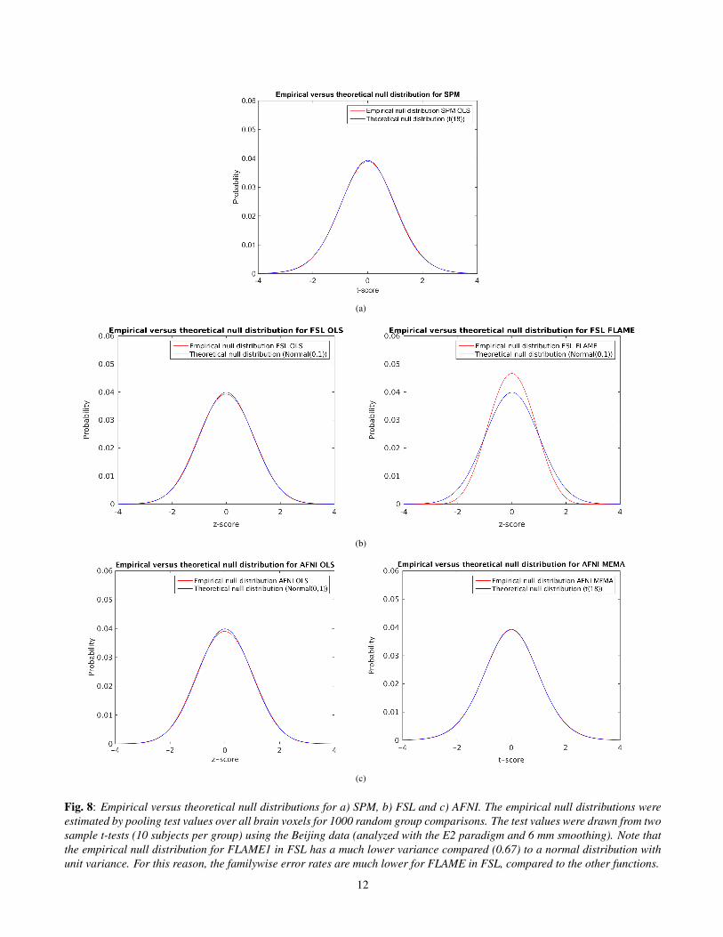
As a first step to understand the inaccuracies in the para-metric methods, the test statistic values (t- or z-scores, asgenerated by each package) were compared to their theoret-ical null distributions. Figure 8 shows the histogram of allbrain voxels for 1000 group analyses (see caption for details).The empirical and theoretical nulls are well-matched, exceptfor FSL’s FLAME1 which has lower variance (σ2 = 0.67)than the theoretical null. This is the proximal cause of thehighly conservative results from FSL FLAME. The mixedeffects variance is composed of intra- and inter-subject vari-ance (σ2

WTN , σ2BTW , respectively), and while other software

packages do not separately estimate each (SPM, FSL OLS),FLAME estimates each and constrains σ2

BTW to be positive.In this null data, the true effect in each subject is zero andthus the true σ2

BTW = 0. Thus unless FLAME’s σ2BWT is

correctly estimated to be 0, it can only be positively biased,and in fact this point was raised by the original authors [30].Additionally, FLAME1 (the currently recommended option)uses a conservative degrees of freedom estimate in lieu of amore accurate but slow degrees of freedom estimation used

Fig. 7: Results for two-sample t-test and ad-hoc cluster-wiseinference, showing estimated familywise error rates for 4-10mm of smoothing and four different activity paradigms (B1,B2, E1, E2), for SPM, FSL and AFNI. These results are fora total of 20 subjects. Each statistic map was first thresh-olded using a cluster defining threshold of p = 0.001 (uncor-rected for multiple comparisons), and the surviving clusterswere then compared to a cluster extent threshold of 80 mm3.The estimated familywise error rates are simply the numberof analyses with a significant result divided by the number ofanalyses (1000).

10

in FLAME2’s BIDET. These two factors are the most likelyexplanation for the observed conservativeness.

2.3. What does the spatial auto correlation function looklike?

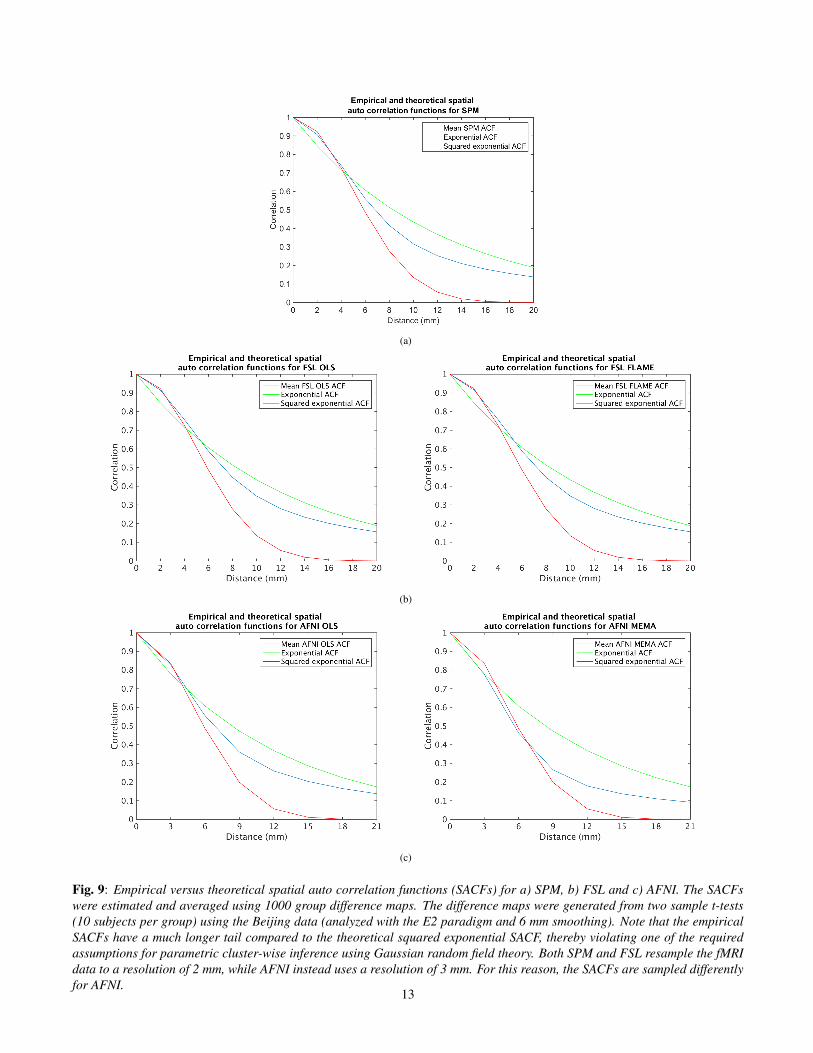
SPM and FSL depend on Gaussian random field theory (RFT)for FWE-corrected voxel-wise and cluster-wise inference.However, RFT cluster-wise inference depends on two addi-tional assumptions. The first assumption is that the spatialsmoothness of the fMRI signal is constant over the brain,and the second assumption is that the spatial auto correlationfunction has a specific shape (a squared exponential) [31]. Toinvestigate the second assumption, the spatial auto correlationfunction was estimated and averaged using 1000 group differ-ence maps. For each group difference map and each distance(1 - 20 mm), the spatial auto correlation was estimated alongx, y and z, by calculating the correlation between the originaldifference map and a shifted version of the difference map.The final estimate is an average of the spatial auto correlationalong x, y and z. The empirical spatial auto correlation func-tions are given in Figure 9. A reference squared exponentialis also included, it is proportional to a Gaussian density withσ = 5 mm, corresponding to an intrinsic smoothness of 8.3mm (FWHM). The empirical spatial auto correlation functionis clearly far from a squared exponential; it has a much longertail. This may explain why the parametric methods workrather well for a high cluster defining threshold (resultingin small clusters) and not as well for a low cluster definingthreshold (resulting in large clusters).

2.4. How do the smoothness estimates and the cluster ex-tent thresholds differ between SPM, FSL and AFNI?

For both voxel and cluster-wise inference, the smoothness ofthe group difference map or group activation map needs to beestimated to calculate the RESEL (resolution element) count,a key parameter for the RFT based p-values. Group modelsmoothness estimates for SPM, FSL FLAME and AFNI, for1000 group comparisons, are given in Figure 10 (see Figurecaption for details). As the preprocessing was unique to eachpackage, it is difficult to make absolute comparisons betweenintrinsic noise smoothness found with each tool. However,the notably lower smoothness estimates from AFNI could bedue to AFNI’s use of first level (intrasubject) residuals insteadof second level (intersubject) residuals like SPM and FSL. Adirect comparison can be made between cluster size thresh-olds of FSL FLAME and a non-parametric test conducted onthe FSL-preprocessed data (see Figure 11), showing the morestringent cluster thresholds the non-parametric method usesto control the familywise error rate.

2.5. Where are the false clusters located in the brain?

To investigate if the false clusters appear randomly in thebrain, all significant clusters (p < 0.05, corrected) were savedas binary maps and summed together, see Figure 13. Thesemaps of voxel-wise cluster frequency show the areas moreand less likely to be marked as significant in a cluster-wiseanalysis (see Figure caption for details). Posterior cingulatewas the most likely area to be covered by a cluster, whilewhite matter was least likely.

To investigate the assumption of a stationary spatialsmoothness, three gradient filters (oriented along x, y and z)were applied to each group difference map, and the averagegradient magnitude

(√(∇x)2 + (∇y)2 + (∇z)2

)(rough-

ness) was calculated over all analyses (while actual analysesuse the residuals, as the null hypothesis is true we can equiv-alently use the statistic maps). The smoothness was finallyobtained as the inverse roughness, and is given in Figure 13.Reductions in smoothness will mean that random clusters aresmaller in size (reducing false positive rate) but also that thereare more clusters (increasing false positive rate); how thesetwo factors balance out are hard to predict.

Clearly, the false clusters appear in spatial patterns thatmatch the degree of smoothness in the group difference maps.For SPM, FSL OLS and AFNI OLS, the degree of smoothnessis correlated with the brain tissue type; the smoothness is gen-erally higher for gray brain tissue compared to white braintissue. This effect has previously been observed for VBMdata [15].

2.6. What is the difference between parametric and non-parametric cluster-wise inference for a typical groupstudy?

All of the analyses to this point have been based on restingstate fMRI data, where the null hypothesis should be true.We now use task data to address the practical question of“How will my FWE-corrected cluster p-values change?” ifa user were to switch from a parametric to a non-parametricmethod. We use four task data sets (rhyme judgment, mixedgambles [32], living-nonliving decision with plain or mirror-reversed text, word and object processing [33]) downloadedfrom the OpenfMRI [9] homepage. The data sets were ana-lyzed using a parametric (the OLS option in FSL’s FEAT) anda non-parametric method (the randomise function in FSL).The only difference between these two methods is that FSLFEAT-OLS relies on Gaussian random field theory to calcu-late the corrected cluster p-values, while randomise insteaduses the data itself. The resulting cluster p-values are givenin Table 3 (cluster defining threshold of p = 0.01) and Ta-bles 4 - 5 (cluster defining threshold of p = 0.001). Figure 14summarizes these results, plotting the ratio of FWE-correctedp-values, non-parametric to parametric, against cluster size.Given the previous null data evaluations showing valid non-

11

(a)

(b)

(c)

Fig. 8: Empirical versus theoretical null distributions for a) SPM, b) FSL and c) AFNI. The empirical null distributions wereestimated by pooling test values over all brain voxels for 1000 random group comparisons. The test values were drawn from twosample t-tests (10 subjects per group) using the Beijing data (analyzed with the E2 paradigm and 6 mm smoothing). Note thatthe empirical null distribution for FLAME1 in FSL has a much lower variance compared (0.67) to a normal distribution withunit variance. For this reason, the familywise error rates are much lower for FLAME in FSL, compared to the other functions.

12

(a)

(b)

(c)

Fig. 9: Empirical versus theoretical spatial auto correlation functions (SACFs) for a) SPM, b) FSL and c) AFNI. The SACFswere estimated and averaged using 1000 group difference maps. The difference maps were generated from two sample t-tests(10 subjects per group) using the Beijing data (analyzed with the E2 paradigm and 6 mm smoothing). Note that the empiricalSACFs have a much longer tail compared to the theoretical squared exponential SACF, thereby violating one of the requiredassumptions for parametric cluster-wise inference using Gaussian random field theory. Both SPM and FSL resample the fMRIdata to a resolution of 2 mm, while AFNI instead uses a resolution of 3 mm. For this reason, the SACFs are sampled differentlyfor AFNI.

13

(a)

(b)

(c)

Fig. 12: The maps show voxel-wise incidence of clusters. Image intensity is the number of times, out of 10,000 random analyses(200,000 for FSL FLAME, to account for fewer clusters per analysis), a cluster occured at a given voxel (CDT p = 0.01), fora) SPM, b) FSL and c) AFNI. Each analysis is a two sample t-test (10 subjects per group) using the Beijing data, analyzed withthe E2 paradigm and 6 mm smoothing. The bright spot in the posterior cingulate corresponds to a region of high smoothness,and suggests non-stationarity as a possible contributing factor.

14

(a)

(b)

(c)

Fig. 13: Maps of inverse spatial gradient magnitude, reflecting the spatial smoothness of the statistic images, for a) SPM, b)FSL and c) AFNI. The smoothness was estimated from 10,000 difference maps generated from two sample t-tests (10 subjectsper group) using the Beijing data (analyzed with the E2 paradigm and 6 mm smoothing). It is clear that the smoothnessvaries spatially; one of the required assumptions for parametric cluster-wise inference using Gaussian random field theory isthereby violated. Note that the bright areas (high smoothness) match the spatial maps of the false clusters; it is more likelyto find a large cluster for areas with a high smoothness. The AFNI software generally results in group difference maps with alower smoothness compared to SPM and FSL. A possible explanation is that AFNI uses higher order interpolation for motioncorrection and spatial normalization, which leads to a lower smoothness compared to more common linear interpolation. Alsonote the reduced smoothness for the iterative methods (FSL FLAME & AFNI 3dMEMA) and their corresponding non-iterativemethods (FSL OLS and AFNI OLS, respectively); the voxel-by-voxel estimation of between subject variance in the iterativemethods reduces the smoothness slightly.

15

Fig. 10: Group smoothness estimates (mm full width at halfmaximum) for SPM, FSL FLAME and AFNI. The smoothnessestimates originate from two sample t-tests (10 subjects pergroup) using the Beijing data (analyzed with the E2 paradigmand 6 mm smoothing). Note that AFNI estimates the groupsmoothness differently compared to SPM and FSL. Also notethat AFNI uses higher order interpolation for motion cor-rection and spatial normalization, which leads to a lowersmoothness compared to more common linear interpolation.

Fig. 11: Cluster extent thresholds (in cubic millimeters) forSPM, FSL FLAME, AFNI and a permutation test, for a clusterdefining threshold of p = 0.01 and a familywise cluster errorrate of p = 0.05. The thresholds originate from two sample t-tests (10 subjects per group) using the Beijing data (analyzedwith the E2 paradigm and 6 mm smoothing). Note that thepermutation threshold can only be directly compared with thethreshold from the FSL software, as first level results fromFSL were used for the non-parametric analyses.

Fig. 14: Ratio of non-parametric to parametric FWE cor-rected p-values for cluster size inference on 4 task (non-null)fMRI datasets, for parametric FWE p-values 0.05 ≥ p ≥10−4. Results for two CDT are shown, p = 0.01 and p= 0.001, and larger ratios indicate parametric p-values be-ing smaller (more significant) than non-parametric p-values(note the logarithmic scale on the y-axis). Clusters with aparametric FWE p-value more significant than 10−4 are ex-cluded because a permutation test with 5000 permutationscan only resolve p-values down to 0.0002, and such p-valueswould generate large ratios inherently. These results suggestcluster size inference with a CDT of p = 0.01 has FWE in-flated by 2 to almost 3 orders of magnitude, and a CDT of p= 0.001 has FWE significance inflated by up to 2 orders ofmagnitude.

parametric and invalid parametric cluster size inference, wetake ratios larger than 1.0 as evidence of inflated (biased) sig-nificance in the parametric inferences.

For a cluster defining threshold of p = 0.01 and a clus-ter size of 400 voxels, the non-parametric cluster p-value isapproximately 10 - 100 times larger compared to the para-metric p-value. For a cluster defining threshold of p = 0.001and a cluster size of 100 voxels, the non-parametric clusterp-value is approximately 1.25 - 10 times larger compared tothe parametric p-value. For contrast 1 of the word and objectprocessing task data set (Table 3), one cluster has a paramet-ric p-value of 0.0182 and a non-parametric p-value of 0.249.This matches the empirically estimated familywise error rateof FSL OLS, according to Figure 5. These findings indicatethat the problems exist also for task based fMRI data, and notonly for resting state data.

16

3. DISCUSSION

Our results clearly show that the parametric statistical meth-ods used for group fMRI analysis with the packages SPM,FSL and AFNI can produce FWE-corrected cluster p-valuesthat are erroneous, being spuriously low and inflating statisti-cal significance. This calls into question the validity of count-less published fMRI studies based on parametric cluster-wiseinference. It is important to stress that we have focused oninferences corrected for multiple comparisons in each groupanalysis, yet some 40% of a sample of 241 recent fMRI pa-pers did not report correcting for multiple comparisons [27],meaning that many group results in the fMRI literature suffereven worse false positive rates than found here [34]. A possi-ble explanation for the lack of multiple comparison correctionis that the correction methods are believed to be too conser-vative, resulting in familywise error rates far below the ex-pected 5%. However, we have found that correction methodsbased on parametric assumptions can actually be very liberalfor cluster-wise inference, yielding familywise error rates ofup to 60%.

Compared to our previous work [16], the results presentedhere are more important for three reasons. First, the cur-rent study considers group analyses, while our previous studylooked at single subject analyses. Group analyses are muchmore common in the fMRI field, and are essential for draw-ing conclusions that should generalize to a population. Sec-ond, we here investigate the validity of the three most com-mon fMRI software packages [27], while we only consideredSPM in our previous study. Third, the non-parametric permu-tation test gives valid results for all two sample t-tests, and for60% of the one sample t-tests. This may be due to violationsof the stronger assumptions of the one-sided permutation testwhich assumes symmetrically distributed errors, in contrast toa two-sample permutation test that only assumes exchange-able errors [25]. In our previous study, the permutation testonly performed well in some cases (mainly because singlesubject fMRI data contain temporal auto correlation whichneeds to be removed prior to permuting the volumes). Forgroup analyses, the brain activity of each subject can be seenas independent, and thus justifies the permutation’s exchange-ability assumption.

3.1. Should resting state data be used to test statistical as-sumptions?

One possible criticism is that resting state fMRI data does nottruly compromise null data, as it may be affected by consistenttrends or transients, for example, at the start of the session.If this was the case, the excess false positives would appearonly in certain paradigms and, in particular, least likely inthe randomized event-related (E2) design. Rather, the inflatedfalse positives were observed across all experiment types withparametric cluster size inference, implying this effect cannot

be responsible.

3.2. Why is cluster-wise inference more problematic thanvoxel-wise?

It is clear that the parametric statistical methods work well, ifconservatively, for voxel-wise inference, but not for cluster-wise inference. We note that other authors have found randomfield theory cluster-wise inference to be invalid in certain set-tings under stationarity [31, 24] and non-stationarity [35, 15].This present work, however, is the most comprehensive toexplore the typical parameters used in task fMRI for a va-riety of software tools. Our results are also corroboratedby similar experiments for structural brain analysis (voxelbased morphometry, VBM) [13, 14, 15, 21, 36], showingthat cluster based p-values are more sensitive to the statis-tical assumptions. For voxel-wise inference, our results areconsistent with a previous comparison between paramet-ric and non-parametric methods for fMRI, showing that anon-parametric permutation test results in lower significancethresholds [15, 37].

Both SPM and FSL rely on RFT to correct for multi-ple comparisons. For voxel-wise inference, RFT is based onthe assumption that the activity map is sufficiently smooth(roughly, at least 3 voxel FWHM [31]), and that the spa-tial auto correlation function (SACF) is twice-differentiableat the origin. Further, RFT is only accurate for sufficient largestatistic values (precisely, a statistic value used as a thresholdwould produce at most one peak under the null hypothesison average). For cluster-wise inference, RFT additionally as-sumes a Gaussian shape of the SACF (i.e. a squared exponen-tial covariance function), and that the spatial smoothness isconstant over the brain. The cluster defining threshold (CDT)must also be sufficiently large, but to accomodate a differ-ent sets of approximations. First, it must be large enough toensure that handles or voids in the clusters do not occur on av-erage (which is much lower than needed for voxel-wise RFTaccuracy), ensuring that the expected Euler characteristic isa good approximation to the (null) expected number of clus-ters. Second, the CDT must be large enough for the (null)distribution of cluster size to be accurate. Note that both SPMand FSL apply cluster size results for Gaussian images to Timages after Gaussianizing the CDT, even though there areT image results available [38]. Hayasaka and Nichols [31]found that the proper T results did not dramatically improvethe performance of the RFT cluster size inferences.

The 3dClustSim function in AFNI also assumes a constantspatial smoothness and a Gaussian form of the SACF (sincea Gaussian smoothing is applied to each generated noise vol-ume). The Monte Carlo approach should be accurate for anyCDT as the other assumptions hold. As the familywise errorrates are far above the expected 5% for cluster-wise inference,but not for voxel-wise inference, one or more of the GaussianSACF, the stationary SACF, or the sufficiently large CDT as-

17

sumptions must be invalid. Cluster-wise inference was dis-couraged for VBM already 15 years ago [14], due to non-stationary spatial smoothness in the statistical maps. The non-stationary smoothness can be modeled [35], but parametricmethods still give invalid results for VBM with low smooth-ing and CDT [15]. In the fMRI field, however, the assumptionof a stationary spatial smoothness has not really been investi-gated.

Figure 9 shows that the SACF is far from a squared expo-nential. The empirical SACFs are close to a squared exponen-tial for small distances, but the auto correlation is higher thanexpected for large distances. This could be the reason whythe parametric methods work rather well for a high clusterdefining threshold (p = 0.001), and not at all for a low thresh-old (p = 0.01). A low threshold gives large clusters with alarge radius, for which the tail of the SACF is quite important.For a high threshold, resulting in rather small clusters with asmall radius, the tail is not as important. Also, it could sim-ply be that the high-threshold assumption is not satisfied fora CDT of p = 0.01. Figure 13 shows that the spatial smooth-ness is not constant in the brain, but varies spatially. Note thatthe bright areas match the spatial distribution of false clus-ters in Figure 12; it is more likely to find a large cluster for ahigh smoothness. The permutation test does not assume a spe-cific shape of the SACF, nor does it assume a constant spatialsmoothness, nor require a high CDT. For these reasons, thepermutation test provides valid results, for two sample t-tests,for both voxel and cluster-wise inference.

3.3. Why does AFNI’s Monte Carlo approach, with fewerparametric assumptions, not perform better?

As can be observed in Figures 1, 2, 4 and 5, AFNI results infamilywise error rates that are high even for a cluster defin-ing threshold of p = 0.001. There are two main factors thatexplain these results.

Firstly, AFNI estimates the spatial group smoothness dif-ferently compared to SPM and FSL. AFNI averages smooth-ness estimates from the first level analysis, whereas SPM andFSL estimate the group smoothness using the group residualsfrom the general linear model [39]. The group smoothnessused by 3dClustSim may for this reason be too low (comparedto SPM and FSL, see Figure 10); the variation of smoothnessover subjects is not considered.

Secondly, a 15 year old bug was found in 3dClustSimwhile testing the three software packages (the bug was fixedby the AFNI group as of May 20151, during preparation ofthis manuscript). The effect of the bug was an underestima-tion of how likely it is to find a cluster of a certain size (inother words, the p-values reported by 3dClustSim were toolow). The main idea behind the 3dClustSim function is togenerate Gaussian noise with unit variance, and then smoothit using a Gaussian lowpass filter with a size corresponding to

1http://afni.nimh.nih.gov/pub/dist/doc/program help/3dClustSim.html

the estimated group smoothness. This procedure is repeated alarge number of times, to obtain an estimate of how commondifferent cluster sizes are for Gaussian noise. The smoothednoise is rescaled back to unit variance, and 3dClustSim per-forms the rescaling by first estimating the variance of thesmoothed noise. Due to edge effects caused by the smoothingoperation the boundary of the volume is attenuated, whichhas two effects. First, the estimated variance used for stan-dardization will be biased down, increasing the variance ofthe simulated images2. Second, the attenuation will reducethe chance that clusters will ever occur near the boundary, ef-fectively reducing the search volume and under estimating theseverity of the multiple testing problem.

Together, the lower group smoothness and the bug in3dClustSim resulted in cluster extent thresholds that aremuch lower compared to SPM and FSL, see Figure 11, whichresulted in particularly high familywise error rates. Note thatthe cluster extent thresholds for SPM, FSL and AFNI matchthe degree of false positives according to Figure 1 (d). AFNIhas the lowest cluster extent thresholds, and therefore resultsin a higher familywise error rate compared to SPM and FSL.FSL has higher extent thresholds compared to SPM, and thefamilywise error rates are therefore slightly lower.

The familywise error rates for AFNI will be lower withthe fixed 3dClustSim function, especially for high levels ofsmoothing (for which the bug in 3dClustSim is more notice-able). As an example of the difference between the old andthe new 3dClustSim function, the new function gives a clusterextent threshold that is 15% higher compared to the old func-tion (for a smoothness of 8 mm). These findings are ratheralarming, as 3dClustSim is one of the most popular choicesfor multiple comparison correction [27].

3.4. Which parameters affect the familywise error ratefor cluster-wise inference?

According to Figures 1, 2, 4 and 5, the cluster defining thresh-old is the most important parameter for SPM, FSL and AFNI;using a more liberal threshold increases the degree of falsepositives. This result is consistent with previous work [15, 24,40]. However, the permutation test is completely unaffectedby changes of this parameter. According to a recent reviewlooking at 484 fMRI studies [24], the used cluster definingthreshold varies greatly between the three software packages(mainly due to different default settings). For SPM, p = 0.001is the default and most common threshold (used in about 70%of the studies), followed by 20% for p = 0.005 and 5% forp = 0.01. For FSL, p = 0.01 is the default and most com-mon choice (65% of the studies), followed by 20% for p =0.001 and 10% greater than p = 0.01. The AFNI software

2The variance of independent unit variance noise after convolution isequal to the sum of squares of the smoothing kernel; this result is not usedby 3dClustSim, which instead uses the empirical variance over the image tostandardize the images.

18

does not have a default setting for the 3dClustSim function,but a threshold of p = 0.005 seems to be the most commonoption (used in 40% of the studies), followed by 25% for p =0.001 and 15% for p = 0.01.

The amount of smoothing has a rather large impact on thedegree of false positives, especially for FSL OLS. The resultsfrom the permutation test, on the other hand, do not depend onthis parameter. The original fMRI data has an intrinsic SACF,which is mixed with the SACF of the smoothing kernel. Thecombined SACF will more closely resemble a squared ex-ponential for high levels of smoothing, simply because thesmoothing operation forces the data to have a more GaussianSACF. The permutation test does not assume a specific formof the SACF, and therefore performs well for any degree ofsmoothing. It should be stressed that AFNI uses 4 mm as thedefault amount of smoothing, while FSL uses 5 mm and SPMuses 8 mm. Both FSL and AFNI OLS show interaction be-tween the amount of smoothing and the fMRI data. For allsoftware packages, the amount of smoothing has a larger ef-fect on the block based activity paradigms, compared to theevent related ones. These two effects are consistent with ourprevious work [16]. SPM, FSL OLS and AFNI also showinteraction between the amount of smoothing and the clusterdefining threshold.

Just as for our previous study [16], the used (pretended)activity paradigm significantly affects the degree of false pos-itives. This was unexpected, but it means that problems thatarise due to temporally correlated noise actually propagatefrom the single subject analysis to the group analysis. SPM,FSL and AFNI 3dMEMA show interaction between the fMRIdata and the activity paradigm. This can be explained by thefact that the Beijing data sets were collected with a repeti-tion time of 2 seconds, while the Cambridge data sets werecollected with a repetition time of 3 seconds. The temporalauto correlation between two consecutive volumes increaseswith the sampling rate, and in our previous study about singlesubject fMRI analysis [16], the sampling rate was found tobe the most important factor for the degree of false positives.Block based designs are more sensitive to temporal auto cor-relations resembling power spectra with an 1/f appearance (fbeing frequency), as their power spectra are concentrated atlow frequencies. The permutation test is unaffected by theused activity paradigm for two sample t-tests, but slightly af-fected for one sample t-tests. An unexpected result is that allsoftware packages show significant interaction between theactivity paradigm and the number of subjects.

All software packages are significantly affected by theanalysis type; the familywise error rates are generally lowerfor a two-sample t-test compared to a one sample t-test. Thiseffect can be explained by the fact that a test value that rep-resents a difference (e.g. the difference in brain activationbetween two groups) can more easily be approximated witha normal distribution, compared to a test value that does notrepresent a difference. As can be seen in Figures 2, 3, 5 and 6,

the one-sample t-tests are problematic even for the permuta-tion test. For both FSL OLS and AFNI, there is strong in-teraction between the analysis type and the fMRI data. Apossible explanation is that the one sample t-tests are moreproblematic for fMRI data collected with a higher samplingrate, as such data have stronger temporal auto correlation be-tween two consecutive volumes [16].

Both FSL FLAME1 and AFNI OLS give a higher de-gree of false positives when the number of subjects increases.This is counter intuitive, as Gaussian random field theory nor-mally works better for higher degrees of freedom. All soft-ware packages except SPM also show interaction between thefMRI data and the number of subjects.

3.5. The future of fMRI

It is not realistic to redo 28,000 fMRI studies, or to re-analyzeall the data. Considering that it is now possible to evaluatecommon statistical methods using real fMRI data, the fMRIcommunity should, in our opinion, focus on validation of ex-isting methods (rather than developing new methods basedon questionable assumptions). A plethora of excellent meth-ods are available in the statistics field, but are seldom used inthe neuroimaging community. A non-parametric permutationtest, for example, is based on a small number of assumptions,and has here been proven to yield more accurate results thanparametric methods. The main drawback of a permutationtest is the increase in computational complexity, as the groupanalysis needs to be repeated 1,000 - 10,000 times. The in-crease in processing time is no longer a problem; an ordinarydesktop computer can run a permutation test for neuroimag-ing data in less than a minute [28, 41]. A single desktop com-puter, with a powerful graphics card, was used in this studyto run all the 384,000 permutation tests (with 1,000 permuta-tions each) in about 15 days (the processing time would be 10- 30 years if the function randomise in FSL was used instead).

In addition to unreliable statistical methods, the neu-roimaging field also suffers from studies having low sta-tistical power [42, 43]. One possible way to increase thestatistical power is to use locally multivariate statistical meth-ods [44, 45, 46, 47, 48], which do not analyze the data onevoxel at a time. Multivariate statistical methods can, how-ever, result in more complicated null distributions, makingit harder to obtain p-values. More advanced clustering tech-niques, such as cluster mass inference [49] or threshold freecluster enhancement [50], can also result in a higher statisticalpower, but it is often hard to derive a theoretical null distribu-tion. A permutation test can estimate the null distribution ofany test statistic, and can thus increase both the accuracy andthe statistical power of fMRI studies.

19

AcknowledgmentThis research was supported by the neuroeconomic researchinitiative at Linkoping university, and by the Swedish researchcouncil (grant 2013-5229 ’statistical analysis of fMRI data’).This study would not be possible without the recent data shar-ing initiatives in the neuroimaging field. We therefore thankthe Neuroimaging Informatics Tools and Resources Clearing-house (NITRC) and all the researchers that have contributedwith resting state data to the 1000 functional connectomesproject. We would also like to thank Russ Poldrack and hiscolleagues for starting the OpenfMRI project (supported byNSF grant OCI-1131441) and all the researchers that haveshared their task based data. The Nvidia corporation, whodonated the Tesla K40 graphics card used to run all the per-mutation tests, is also acknowledged.

4. REFERENCES

[1] Ogawa, S. et al., “Intrinsic signal changes accompany-ing sensory stimulation: functional brain mapping withmagnetic resonance imaging,” PNAS, vol. 89, pp. 5951–5955, 1992.

[2] N.K. Logothetis, “What we can do and what we cannotdo with fMRI,” Nature, vol. 453, pp. 869–878, 2008.

[3] B. Biswal, F. Zerrin Yetkin, V. M. Haughton, and J. S.Hyde, “Functional connectivity in the motor cortex ofresting human brain using echo-planar MRI,” Magneticresonance in medicine, vol. 34, pp. 537–541, 1995.

[4] Hutchison, R.M. et al., “Dynamic functional connectiv-ity: Promise, issues, and interpretations,” NeuroImage,vol. 80, pp. 360 – 378, 2013.

[5] M. Welvaert and Y. Rosseel, “A review of fMRI simu-lation studies,” PLoS ONE, vol. 9, pp. e101953, 2014.

[6] Biswal, B. et al., “Toward discovery science of humanbrain function,” PNAS, vol. 107, pp. 4734–4739, 2010.

[7] Van Essen, D. et al., “The WU-Minn Human Connec-tome Project: An overview,” NeuroImage, vol. 80, pp.62–79, 2013.

[8] R. Poldrack and K. Gorgolewski, “Making big dataopen: data sharing in neuroimaging,” Nature Neuro-science, vol. 17, pp. 1510–1517, 2014.

[9] Poldrack, R. et al., “Toward open sharing of task-basedfMRI data: the OpenfMRI project,” Frontiers in Neu-roinformatics, vol. 7, no. 12, 2013.

[10] Mueller, S.G. et al., “The Alzheimer’s disease neu-roimaging initiative,” Neuroimaging Clinics of NorthAmerica, vol. 15, no. 4, pp. 869 – 877, 2005.

[11] Jack, C.R. et al., “The Alzheimer’s disease neuroimag-ing initiative (ADNI): MRI methods,” Journal of Mag-netic Resonance Imaging, vol. 27, no. 4, pp. 685–691,2008.

[12] Poline, J.B. et al., “Data sharing in neuroimaging re-search,” Frontiers in Neuroinformatics, vol. 6, no. 9,2012.

[13] C. Scarpazza, G. Sartori, M. de Simone, andA. Mechelli, “When the single matters more than thegroup: very high false positive rates in single case voxelbased morphometry,” NeuroImage, vol. 70, pp. 175–188, 2013.

[14] J. Ashburner and K. Friston, “Voxel-based morphome-try - the methods,” NeuroImage, vol. 11, pp. 805–821,2000.

[15] M. Silver, G. Montana, and T. Nichols, “False positivesin neuroimaging genetics using voxel-based morphom-etry data,” NeuroImage, vol. 54, pp. 992–1000, 2011.

[16] A. Eklund, M. Andersson, C. Josephson, M. Johannes-son, and H. Knutsson, “Does parametric fMRI analysiswith SPM yield valid results? - An empirical study of1484 rest datasets,” NeuroImage, vol. 61, pp. 565–578,2012.

[17] K. Friston, J. Ashburner, S. Kiebel, T. Nichols, andW. Penny, Statistical Parametric Mapping: the Analysisof Functional Brain Images, Elsevier/Academic Press,2007.

[18] J. Ashburner, “SPM: a history,” NeuroImage, vol. 62,pp. 791–800, 2012.

[19] M. Jenkinson, C. Beckmann, T. Behrens, M. Woolrich,and S. Smith, “FSL,” NeuroImage, vol. 62, pp. 782–790,2012.

[20] R. W. Cox, “AFNI: Software for analysis and visual-ization of functional magnetic resonance neuroimages,”Computers and Biomedical Research, vol. 29, pp. 162–173, 1996.

[21] C. Scarpazza, S. Tognin, S. Frisciata, G. Sartori, andA. Mechelli, “False positive rates in voxel-based mor-phometry studies of the human brain: Should we beworried?,” Neuroscience & Biobehavioral Reviews, vol.52, pp. 49–55, 2015.

[22] K. J. Friston, K. J. Worsley, R. S. J. Frackowiak, J. C.Mazziotta, and A. C. Evans, “Assessing the significanceof focal activations using their spatial extent,” HumanBrain Mapping, vol. 1, pp. 210–220, 1994.

20

[23] Forman, S. D. et al., “Improved assessment of signifi-cant activation in functional magnetic resonance imag-ing (fMRI): Use of a cluster-size threshold,” Magneticresonance in medicine, vol. 33, pp. 636–647, 1995.

[24] C. Woo, A. Krishnan, and T. Wager, “Cluster-extentbased thresholding in fMRI analyses: Pitfalls and rec-ommendations,” NeuroImage, vol. 91, pp. 412 – 419,2014.

[25] T.E. Nichols and A.P. Holmes, “Nonparametric permu-tation tests for functional neuroimaging: a primer withexamples,” Human brain mapping, vol. 15, pp. 1–25,2002.

[26] A. Winkler, G. Ridgway, M. Webster, S. Smith, andT. Nichols, “Permutation inference for the general linearmodel,” NeuroImage, vol. 92, pp. 381–397, 2014.

[27] J. Carp, “The secret lives of experiments: Methods re-porting in the fMRI literature,” NeuroImage, vol. 63, pp.289–300, 2012.

[28] A. Eklund, P. Dufort, M. Villani, and S. LaConte,“BROCCOLI: Software for fast fMRI analysis on many-core CPUs and GPUs,” Frontiers in Neuroinformatics,vol. 8:24, 2014.

[29] M.D. Lieberman and W.A. Cunningham, “Type I andType II error concerns in fMRI research: re-balancingthe scale,” Social cognitive and affective neuroscience,vol. 4, pp. 423–428, 2009.

[30] M. Woolrich, T. Behrens, C. Beckmann, M. Jenkinson,and S. Smith, “Multilevel linear modelling for FMRIgroup analysis using Bayesian inference,” NeuroImage,vol. 21, pp. 1732–1747, 2004.

[31] S. Hayasaka and T.E. Nichols, “Validating clustersize inference: random field and permutation methods,”NeuroImage, vol. 20, pp. 2343–2356, 2003.

[32] S.M. Tom, C.R. Fox, C. Trepel, and R.A. Poldrack,“The neural basis of loss aversion in decision-makingunder risk,” Science, vol. 315, pp. 515–518, 2007.

[33] K.J. Duncan, C. Pattamadilok, I. Knierim, and J.T. De-vlin, “Consistency and variability in functional localis-ers,” NeuroImage, vol. 46, pp. 1018–1026, 2009.

[34] J.P. A. Ioannidis, “Why most published research find-ings are false,” PLOS Medicine, vol. 2, pp. e124, 2005.

[35] S. Hayasakaa, K. L. Phanb, I. Liberzonc, K. J. Worsley,and T. E. Nichols, “Nonstationary cluster-size inferencewith random field and permutation methods,” NeuroIm-age, vol. 22, pp. 676–687, 2004.

[36] Meyer-Lindenberg, A. et al., “False positives in imaginggenetics,” NeuroImage, vol. 40, pp. 655–661, 2008.

[37] T. Nichols, “Controlling the familywise error rate infunctional neuroimaging: a comparative review,” Statis-tical methods in medical research, vol. 12, pp. 419–446,2003.

[38] J. Cao and K. Worsley, “Applications of random fieldsin human brain mapping,” in Spatial Statistics: Method-ological Aspects and Applications, M. Moore, Ed., pp.169–182. Springer, New York, 2001.

[39] S.J. Kiebel, J.-B. Poline, K.J. Friston, A.P. Holmes, andK.J. Worsley, “Robust smoothness estimation in statis-tical parametric maps using standardized residuals fromthe general linear model,” NeuroImage, vol. 10, pp.756–766, 1999.

[40] A. Eklund, T. Nichols, M. Andersson, and H. Knutsson,“Empirically investigating the statistical validity ofSPM, FSL and AFNI for single subject fMRI analysis,”in IEEE International symposium on biomedical imag-ing (ISBI), 2015, pp. 1376–1380.

[41] A. Eklund, P. Dufort, D. Forsberg, and S. LaConte,“Medical image processing on the GPU - Past, presentand future,” Medical Image Analysis, vol. 17, pp. 1073–1094, 2013.

[42] Button, K.S. et al., “Power failure: why small samplesize undermines the reliability of neuroscience,” NatureReviews Neuroscience, vol. 14, pp. 365–376, 2013.

[43] J. Durnez, B. Moerkerke, and T. Nichols, “Post-hocpower estimation for topological inference in fMRI,”NeuroImage, vol. 84, pp. 45–64, 2014.

[44] O. Friman, M. Borga, P. Lundberg, and H. Knutsson,“Adaptive analysis of fMRI data,” NeuroImage, vol. 19,pp. 837–845, 2003.

[45] A. Eklund, M. Andersson, and H. Knutsson, “Fastrandom permutation tests enable objective evaluationof methods for single-subject fMRI analysis,” Inter-national Journal of Biomedical Imaging, Article ID627947, vol. 2011, 2011.

[46] M. Bjornsdotter, K. Rylander, and J. Wessberg, “AMonte Carlo method for locally multivariate brain map-ping,” NeuroImage, vol. 56, pp. 508–516, 2011.

[47] M. Jin, R. Nandy, T. Curran, and D. Cordes, “Extendinglocal canonical correlation analysis to handle generallinear contrasts for fMRI data,” International Journalof Biomedical Imaging, Article ID 574971, vol. 2012,2012.

21

[48] J.A. Etzel, J.M. Zacks, and T.S. Braver, “Searchlightanalysis: Promise, pitfalls, and potential,” NeuroImage,vol. 78, pp. 261 – 269, 2013.

[49] H. Zhang, T.E. Nichols, and T.D. Johnson, “Clustermass inference via random field theory,” NeuroImage,vol. 44, pp. 51 – 61, 2009.

[50] S.M. Smith and T.E. Nichols, “Threshold-free clus-ter enhancement: Addressing problems of smoothing,threshold dependence and localisation in cluster infer-ence,” NeuroImage, vol. 44, pp. 83–98, 2009.

22

5. METHODS

5.1. Resting state fMRI data

Resting state fMRI data from 396 healthy controls weredownloaded from the homepage of the 1000 functional con-nectomes project [6](http://fcon 1000.projects.nitrc.org/fcpClassic/FcpTable.html).The Beijing and the Cambridge data sets were selected fortheir large sample sizes (198 subjects each) and their narrowage ranges (21.2 ± 1.8 and 21.0 ± 2.3 years, respectively).The Beijing data were collected with a repetition time (TR)of 2 seconds and consist of 225 time points per subject, thespatial resolution is 3.125 x 3.125 x 3.6 mm3. The Cambridgedata were collected with a TR of 3 seconds and consist of 119time points per subject, the spatial resolution is 3 x 3 x 3mm3. For each subject there is one T1-weighted anatomi-cal volume which can be used for normalization to a braintemplate. According to the motion plots from FSL, no sub-ject moved more than 1 mm in any direction. According tomotion plots from AFNI, one Cambridge subject and threeBeijing subjects moved slightly more than 1 mm. The fMRIdata have not been corrected for geometric distortions, andno field maps are available for this purpose.

Since all the subjects are healthy and of similar age, itshould be impossible to find any significant brain activity dif-ferences between two randomly generated subgroups (anal-yses were performed separately for the Beijing data and theCambridge data). The same approach has previously beenused to test the validity of parametric statistics for voxel basedmorphometry [14, 21]. As the subjects have not performedany specific task in the MR scanner, it should also be impos-sible to find significant group activations. The data can thusbe used to test both two-sample t-tests (group differences) andone sample t-tests (group activations).

5.1.1. Random group generation

Each random group was created by first applying a randompermutation to a list containing all the 198 subject numbers.To create two random groups of 20 subjects each, the first 20permuted subject numbers were put into group 1, and the fol-lowing 20 permuted subject numbers were put into group 2.According to the n choose k formula n!

k!(n−k)! it is possible tocreate approximately 1.31 ·1042 such random group divisions(n = 198 and k = 40). The analyses will not be independent,but the estimate of the familywise false positive rate will stillbe unbiased. A total of 1000 random analyses were used to es-timate the familywise false positive rate, giving a 95% confi-dence interval of 3.65% - 6.35% for an expected false positiverate of 5%. To make a fair comparison between the differentsoftware packages, the same 1000 permutations were used forall software packages and all parameter settings.

5.1.2. Code availability

Parametric group analyses were performed using SPM 8(http://www.fil.ion.ucl.ac.uk/spm/software/spm8/), FSL 5.0.7(http://fsl.fmrib.ox.ac.uk/fsldownloads/) and AFNI(http://afni.nimh.nih.gov/afni/download/afni/releases, com-piled August 13 2014, version 2011 12 21 1014). FSL canperform non-parametric group analyses using the functionrandomise, but we here used our BROCCOLI software [28](https://github.com/wanderine/BROCCOLI) to lower the pro-cessing time. All the processing scripts are freely available(https://github.com/wanderine/ParametricMultisubjectfMRI)to show all the processing settings and to facilitate replicationof the results. Since all the software packages and all thefMRI data are also freely available, anyone can replicate theresults in this paper.

5.1.3. First level analyses

A first processing script was used for each software pack-age to perform first level analyses for each subject, resultingin brain activation maps in a standard brain space (MontrealNeurological Institute (MNI) for SPM and FSL, and Talairachfor AFNI). All first level analyses involved normalization toa brain template, motion correction and different amounts ofsmoothing (4, 6, 8 and 10 mm full width at half maximum).Slice timing correction was not performed, as the slice timinginformation is not available in the fMRI data sets. A generallinear model (GLM) was finally applied to the preprocessedfMRI data, using different regressors for activity (B1, B2, E1,E2). The estimated head motion parameters were used as ad-ditional regressors in the design matrix, for all packages, tofurther reduce effects of head motion.

First level analyses were for SPM performed using a Mat-lab batch script, mainly created using the SPM manual. Thespatial normalization was done as a two step procedure, wherethe mean fMRI volume was first aligned to the anatomicalvolume (using the function ’Coregister’ with default settings).The anatomical volume was aligned to MNI space using thefunction ’Segment’ (with default settings), and the two trans-forms were finally combined to transform the fMRI data toMNI space at 2 mm isotropic resolution (using the function’Normalise: Write’). Spatial smoothing was finally appliedto the spatially normalized fMRI data. The first level modelswere then fit in the atlas space, i.e. not in the subject space.

For FSL, first level analyses were setup through theFEAT GUI. The spatial normalization to the brain tem-plate (MNI152 T1 2mm brain.nii.gz) was performed as atwo step linear registration using the function FLIRT (whichis the default option). One fMRI volume was aligned to theanatomical volume using the BBR (boundary based regis-tration) option in FLIRT (default). The anatomical volumewas aligned to MNI space using a linear registration with12 degrees of freedom (default), and the two transforms werefinally combined. The first level models were fit in the subject

23

space (after spatial smoothing), and the contrasts and theirvariances were then transformed to the atlas space.

First level analyses in AFNI were performed using thestandardized processing script afni proc.py, which creates atcsh script which contains all the calls to different AFNI func-tions. The spatial normalization was performed as a two stepprocedure. One fMRI volume was first linearly aligned to theanatomical volume, using the script align epi anat.py. Theanatomical volume was then linearly aligned to the brain tem-plate (TT N27+tlrc) using the script @auto tlrc. The transfor-mations from the spatial normalization and the motion correc-tion were finally applied using a single interpolation, result-ing in normalized fMRI data in an isotropic resolution of 3mm. Spatial smoothing was applied to the spatially normal-ized fMRI data, and the first level models were then fit in theatlas space (i.e. not in the subject space).

Default drift modelling or highpass filtering options wereused in each of SPM, FSL and AFNI. A discrete cosine trans-form with cutoff of 128 seconds was used for SPM, whilehighpass filters with different cutoffs where used for FSL (20seconds for activity paradigm B1, 60 seconds for B2 and 100seconds for E1 and E2), matching the defaults used by theFEAT GUI, and AFNI’s Legende polynomial order is 4 and3 for the Beijing and the Cambridge data, respectively (basedon total scan duration). Temporal correlations were furthercorrected for with a global AR(1) model in SPM, an arbitrarytemporal auto correlation function regularized with a Tukeytaper and adaptive spatial smoothing in FSL and a voxel-wiseARMA(1,1) model in AFNI.

5.1.4. Group analyses

A second processing script was used for each software pack-age to perform random effect group analyses, using the resultsfrom the first level analyses. For SPM, group analyses wereonly performed with the resulting beta weights from the firstlevel analyses, using ordinary least squares (OLS) regressionover subjects. For FSL, group analyses were performed bothusing FLAME1 (which is the default option) and OLS. TheFLAME1 function uses both the beta weight and the corre-sponding variance of each subject, subsequently estimatinga between subject variance. For AFNI, group analyses wereperformed using the functions 3dttest++ (OLS, using beta es-timates from the function 3dDeconvolve which assumes inde-pendent errors) and 3dMEMA (which is similar to FLAME1in FSL, using beta and variance estimates from the function3dREMLfit which uses a voxel-wise ARMA(1,1) model ofthe errors).

For the non-parametric analyses in BROCCOLI, first levelresults from FSL were used and OLS regression was per-formed in each permutation. The largest test value acrossthe entire brain was saved in each permutation, to empiricallyform the null distribution of the maximum test statistic (whichis required to correct for multiple comparisons). For cluster-

wise inference, the cluster defining threshold was first appliedand the size of the largest cluster was then saved in each per-mutation. A permutation test cannot be used for testing groupactivations (one sample t-tests), as the mean brain activity isinvariant to permutations of the subjects. An alternative isto instead use random sign flipping of the subjects, justifiedby an assumption of symmetrically distributed errors, whichis the solution that FSL and BROCCOLI use for one samplet-tests. Each non-parametric group analysis was performedusing 1000 permutations or sign flips, giving a total of 192million permutations and 192 million sign flips for all groupanalyses (hence the need to lower the processing time).

Voxel-wise FWE-corrected p-values from SPM and FSLwere obtained based on their respective implementations ofrandom field theory, while AFNI FWE p-values were ob-tained with a Bonferroni correction for the number of voxels(AFNI does not provide any specific program for voxel-wiseFWE p-values). For the non-parametric analyses, FWE-corrected p-values were calculated with the empirical nulldistribution of the voxel-wise maximum statistic, computedas the proportion of the null distribution being larger than aparticular statistic value.

Cluster-wise FWE-corrected p-values from SPM and FSLwere likewise obtained based on their implementations of ran-dom field theory. AFNI estimates FWE p-values with a sim-ulation based procedure, 3dClustSim. SPM and FSL estimatesmoothness from the residuals of the group level analysis(used for both voxel-wise and cluster-wise inference), whileAFNI uses the average of the first level analyses’ smoothnessestimates. For the non-parametric analyses, FWE-correctedp-values were calculated as the proportion of cluster sizes inthe empirically estimated null distribution being larger thaneach cluster in the group difference map or group activationmap.

Each group analysis was considered to give a significantresult if any cluster or voxel had a FWE-corrected p-valuep < 0.05.

5.2. Task based fMRI data

Task based fMRI data were downloaded from the homepageof the OpenfMRI project [9] (http://openfmri.org), to inves-tigate how cluster based p-values differ between parametricand non-parametric group analyses. Each task dataset con-tains fMRI data, anatomical data and timing information foreach subject. The data sets were only analyzed with FSL,using 5 mm of smoothing (the default option). Motion re-gressors were used in all cases, to further suppress effects ofhead motion. Group analyses were performed using the para-metric OLS option (i.e. not the default FLAME1 option) andthe non-parametric randomise function.

24

5.2.1. Rhyme judgment

The rhyme judgment dataset is available athttp://openfmri.org/dataset/ds000003. The 13 subjects werepresented with pairs of either words or pseudowords, andmade rhyming judgments for each pair. The fMRI data werecollected with a repetition time of 2 seconds and consist of160 time points per subject, the spatial resolution is 3.125x 3.125 x 4 mm3. The data were analyzed with two regres-sors; one for words and one for pseudo words. A total offour contrasts were applied; words, pseudowords, words -pseudowords, pseudowords - words. For a cluster definingthreshold of p = 0.01, a t-threshold of 2.65 was used. For acluster defining threshold of p = 0.001, a t-threshold of 3.95was used.

5.2.2. Mixed-gambles task

The mixed-gambles task dataset is available athttp://openfmri.org/dataset/ds000005. The 16 subjects werepresented with mixed (gain/loss) gambles, and decidedwhether they would accept each gamble. No outcomes ofthese gambles were presented during scanning, but afterthe scan three gambles were selected at random and playedfor real money. The fMRI data were collected using a 3 TSiemens Allegra scanner. A repetition time of 2 seconds wasused and a total of 240 volumes were collected for each run,the spatial resolution is 3.125 x 3.125 x 4 mm3. The datasetcontains three runs per subject, but only the first run was usedin our analysis. The data were analyzed using four regressors;task, parametric gain, parametric loss and distance from in-difference. A total of four contrasts were applied; parametricgain, - parametric gain, parametric loss, - parametric loss.For a cluster defining threshold of p = 0.01, a t-threshold of2.57 was used. For a cluster defining threshold of p = 0.001,a t-threshold of 3.75 was used.

5.2.3. Living-nonliving decision with plain or mirror-reversedtext

The living-nonliving decision task dataset is available athttp://openfmri.org/dataset/ds000006a. The 14 subjects madeliving-nonliving decisions on items presented in either plainor mirror-reversed text. The fMRI data were collected using a3 T Siemens Allegra scanner. A repetition time of 2 secondswas used and a total of 205 volumes were collected for eachrun, the spatial resolution is 3.125 x 3.125 x 5 mm3. Thedataset contains six runs per subject, but only the first runwas used in our analysis. The data were analyzed using fiveregressors; mirror-switched, mirror-repeat, plain-switched,plain-repeat and junk. A total of four contrasts were ap-plied; mirrored versus plain (1,1,-1,-1,0), switched versusnon-switched (1,-1,1,-1,0), switched versus non-switchedmirrored only (1,-1,0,0,0) and switched versus non-switchedplain only (0,0,1,-1,0). For a cluster defining threshold of p =

0.01, a t-threshold of 2.615 was used. For a cluster definingthreshold of p = 0.001, a t-threshold of = 3.87 was used.

5.2.4. Word and object processing

The word and object processing task dataset is available athttp://openfmri.org/dataset/ds000107. The 49 subjects per-formed a visual one-back task with four categories of items:written words, objects, scrambled objects and consonant letterstrings. The fMRI data were collected using a 1.5 T Siemensscanner. A repetition time of 3 seconds was used and a totalof 165 volumes were collected for each run, the spatial resolu-tion is 3 x 3 x 3 mm3. The dataset contains two runs per sub-ject, but only the first run was used in our analysis. The datawere analyzed using four regressors; words, objects, scram-bled objects, consonant strings. A total of six contrasts wereapplied; words, objects, scrambled objects, consonant strings,objects versus scrambled objects (0,1,-1,0) and words versusconsonant strings (1,0,0,-1). For a cluster defining thresholdof p = 0.01, a t-threshold of 2.38 was used. For a cluster defin-ing threshold of p = 0.001, a t-threshold of 3.28 was used.

25

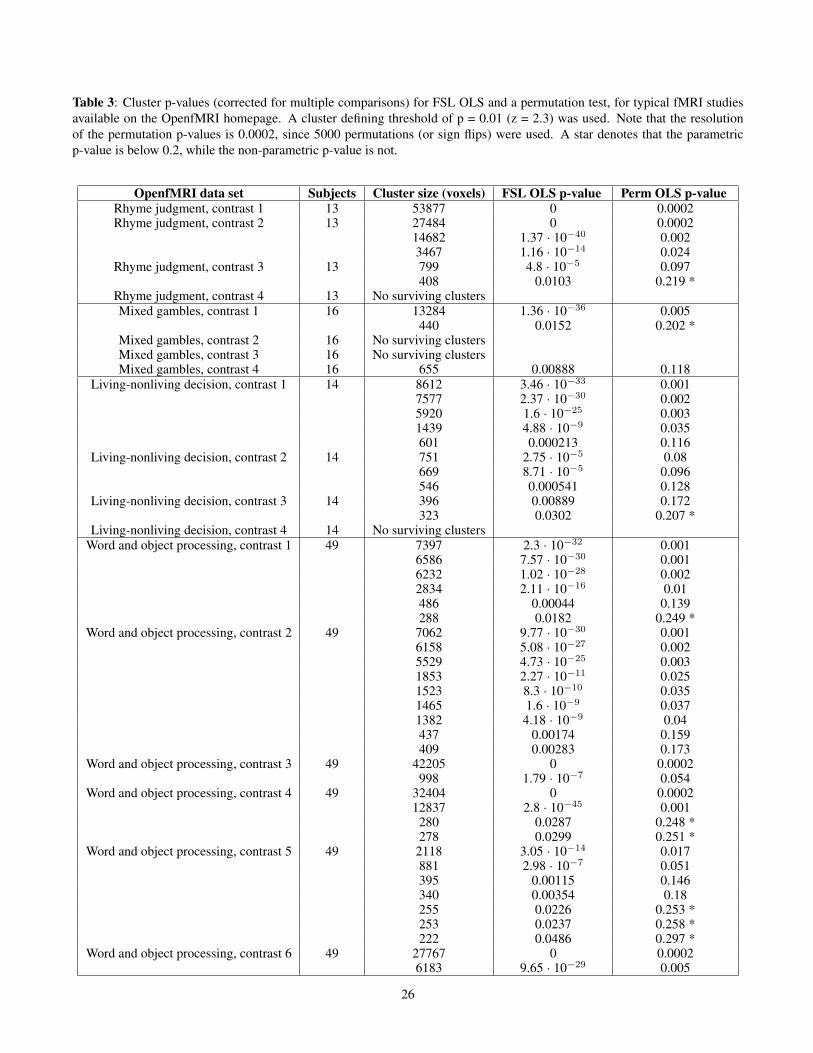
Table 3: Cluster p-values (corrected for multiple comparisons) for FSL OLS and a permutation test, for typical fMRI studiesavailable on the OpenfMRI homepage. A cluster defining threshold of p = 0.01 (z = 2.3) was used. Note that the resolutionof the permutation p-values is 0.0002, since 5000 permutations (or sign flips) were used. A star denotes that the parametricp-value is below 0.2, while the non-parametric p-value is not.

OpenfMRI data set Subjects Cluster size (voxels) FSL OLS p-value Perm OLS p-valueRhyme judgment, contrast 1 13 53877 0 0.0002Rhyme judgment, contrast 2 13 27484 0 0.0002

14682 1.37 · 10−40 0.0023467 1.16 · 10−14 0.024

Rhyme judgment, contrast 3 13 799 4.8 · 10−5 0.097408 0.0103 0.219 *

Rhyme judgment, contrast 4 13 No surviving clustersMixed gambles, contrast 1 16 13284 1.36 · 10−36 0.005

440 0.0152 0.202 *Mixed gambles, contrast 2 16 No surviving clustersMixed gambles, contrast 3 16 No surviving clustersMixed gambles, contrast 4 16 655 0.00888 0.118

Living-nonliving decision, contrast 1 14 8612 3.46 · 10−33 0.0017577 2.37 · 10−30 0.0025920 1.6 · 10−25 0.0031439 4.88 · 10−9 0.035601 0.000213 0.116

Living-nonliving decision, contrast 2 14 751 2.75 · 10−5 0.08669 8.71 · 10−5 0.096546 0.000541 0.128

Living-nonliving decision, contrast 3 14 396 0.00889 0.172323 0.0302 0.207 *

Living-nonliving decision, contrast 4 14 No surviving clustersWord and object processing, contrast 1 49 7397 2.3 · 10−32 0.001

6586 7.57 · 10−30 0.0016232 1.02 · 10−28 0.0022834 2.11 · 10−16 0.01486 0.00044 0.139288 0.0182 0.249 *

Word and object processing, contrast 2 49 7062 9.77 · 10−30 0.0016158 5.08 · 10−27 0.0025529 4.73 · 10−25 0.0031853 2.27 · 10−11 0.0251523 8.3 · 10−10 0.0351465 1.6 · 10−9 0.0371382 4.18 · 10−9 0.04437 0.00174 0.159409 0.00283 0.173

Word and object processing, contrast 3 49 42205 0 0.0002998 1.79 · 10−7 0.054

Word and object processing, contrast 4 49 32404 0 0.000212837 2.8 · 10−45 0.001

280 0.0287 0.248 *278 0.0299 0.251 *

Word and object processing, contrast 5 49 2118 3.05 · 10−14 0.017881 2.98 · 10−7 0.051395 0.00115 0.146340 0.00354 0.18255 0.0226 0.253 *253 0.0237 0.258 *222 0.0486 0.297 *

Word and object processing, contrast 6 49 27767 0 0.00026183 9.65 · 10−29 0.005

26

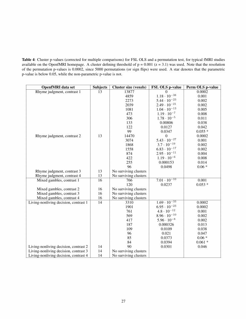
Table 4: Cluster p-values (corrected for multiple comparisons) for FSL OLS and a permutation test, for typical fMRI studiesavailable on the OpenfMRI homepage. A cluster defining threshold of p = 0.001 (z = 3.1) was used. Note that the resolutionof the permutation p-values is 0.0002, since 5000 permutations (or sign flips) were used. A star denotes that the parametricp-value is below 0.05, while the non-parametric p-value is not.

OpenfMRI data set Subjects Cluster size (voxels) FSL OLS p-value Perm OLS p-valueRhyme judgment, contrast 1 13 13877 0 0.0002

4859 1.18 · 10−38 0.0012273 5.44 · 10−23 0.0022039 2.49 · 10−21 0.0021081 1.04 · 10−13 0.005473 1.19 · 10−7 0.008306 1.78 · 10−5 0.011133 0.00806 0.038122 0.0127 0.04299 0.0347 0.055 *

Rhyme judgment, contrast 2 13 14470 0 0.00023074 5.43 · 10−27 0.0011868 3.7 · 10−19 0.0021558 6.83 · 10−17 0.002874 2.95 · 10−11 0.004422 1.19 · 10−6 0.008255 0.000153 0.01496 0.0498 0.06 *

Rhyme judgment, contrast 3 13 No surviving clustersRhyme judgment, contrast 4 13 No surviving clustersMixed gambles, contrast 1 16 766 7.01 · 10−10 0.001

120 0.0237 0.053 *Mixed gambles, contrast 2 16 No surviving clustersMixed gambles, contrast 3 16 No surviving clustersMixed gambles, contrast 4 16 No surviving clusters

Living-nonliving decision, contrast 1 14 3310 1.69 · 10−33 0.00021901 6.95 · 10−23 0.0002761 4.8 · 10−12 0.001569 8.96 · 10−10 0.002417 5.96 · 10−8 0.002187 0.000326 0.013109 0.0109 0.03896 0.021 0.04785 0.0373 0.06 *84 0.0394 0.061 *

Living-nonliving decision, contrast 2 14 90 0.0301 0.046Living-nonliving decision, contrast 3 14 No surviving clustersLiving-nonliving decision, contrast 4 14 No surviving clusters

27

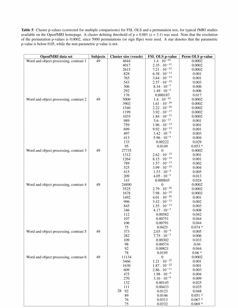
Table 5: Cluster p-values (corrected for multiple comparisons) for FSL OLS and a permutation test, for typical fMRI studiesavailable on the OpenfMRI homepage. A cluster defining threshold of p = 0.001 (z = 3.1) was used. Note that the resolutionof the permutation p-values is 0.0002, since 5000 permutations (or sign flips) were used. A star denotes that the parametricp-value is below 0.05, while the non-parametric p-value is not.

OpenfMRI data set Subjects Cluster size (voxels) FSL OLS p-value Perm OLS p-valueWord and object processing, contrast 1 49 4644 1.4 · 10−45 0.0002

4017 2.35 · 10−41 0.00022615 7.21 · 10−31 0.0002828 6.38 · 10−14 0.001765 3.64 · 10−13 0.001543 2.57 · 10−10 0.003306 8.34 · 10−7 0.006292 1.49 · 10−6 0.006176 0.000187 0.017

Word and object processing, contrast 2 49 5000 1.4 · 10−45 0.00023902 1.61 · 10−38 0.00021540 2.22 · 10−20 0.00021199 3.92 · 10−17 0.00021035 1.84 · 10−15 0.0002989 5.6 · 10−15 0.001759 1.96 · 10−12 0.001699 9.92 · 10−12 0.001497 3.42 · 10−9 0.003413 5.96 · 10−8 0.004133 0.00222 0.02995 0.0149 0.053 *

Word and object processing, contrast 3 49 27735 0 0.00021312 2.62 · 10−19 0.0011264 8.15 · 10−19 0.001789 1.57 · 10−13 0.002525 3.99 · 10−10 0.004415 1.53 · 10−8 0.005209 4.05 · 10−5 0.013143 0.000845 0.024

Word and object processing, contrast 4 49 24890 0 0.00023525 2.79 · 10−36 0.00021678 7.98 · 10−22 0.00021492 4.01 · 10−20 0.001996 3.42 · 10−15 0.002845 1.55 · 10−13 0.003346 4.17 · 10−7 0.008112 0.00582 0.042107 0.00751 0.044106 0.00791 0.04475 0.0425 0.074 *

Word and object processing, contrast 5 49 373 2.03 · 10−8 0.005282 7.75 · 10−7 0.006109 0.00302 0.03398 0.00574 0.0492 0.00821 0.04478 0.0195 0.06 *

Word and object processing, contrast 6 49 11134 0 0.00023466 1.21 · 10−37 0.0011630 1.87 · 10−22 0.001609 2.86 · 10−11 0.003475 1.98 · 10−9 0.004270 3.16 · 10−6 0.009132 0.00145 0.025111 0.00433 0.03592 0.0123 0.04889 0.0146 0.051 *76 0.0313 0.067 *75 0.0332 0.069 *

28