Consiglio Nazionale delle Ricerche

Istituto diMatematica Applicata eTecnologie Informatiche

PUBBLICAZIONI

Enrico Bertolazzi and Gianmarco Manzini

DIAGONALLY IMPLICIT–EXPLICIT RUNGE KUTTA METHODS FORMULTIDIMENSIONAL HYPERBOLIC SYSTEMS.PART II: ANALYSIS AND NUMERICAL EXPERIMENTS.

N. 17-PV 2004

Diagonally Implicit–Explicit Runge Kutta Methodsfor Multidimensional Hyperbolic Systems.

Part II: Analysis and Numerical Experiments.

Enrico Bertolazzia Gianmarco Manzinib

aDipartimento di Ingegneria Meccanica e Strutturale,Universita di Trento,

via Mesiano 77, I – 38050 Trento, ItalybIstituto di Matematica Applicata e Tecnologie Informatiche, IMATI – CNR,

via Ferrata 1, I – 27100 Pavia, Italy

Abstract

In this paper we continue the study of the Diagonally IMplicit-EXplicit Runge-Kutta(DIMEX-RK) methods that we proposed in the first part of this work in the frameworkof Finite Volume methods for unstructured grids. These new numerical approximationschemes are based on a special splitting of the physical and numerical flux vector functionsinto a convective and a non-convective part. In the framework of DIMEX-RK schemes,the convective part is discretized in an implicit way, whilewe discuss the non-convectiveone in an explicit way. We discuss some theoretical properties of the non-linear algebraicevolution operators that are derived in the full discretization from the application of thesemethods to strongly convected dominated flows. A set of numerical experiments illustratesthe behavior of this class of methods on reactive and non-reactive hypersonic simulations.

Key words: Finite Volume, Runge-Kutta, Implicit-Explicit, Partial Differential Equation,M-matrix, Unstructured Grid

1 Introduction

This is the second paper in a series in which we contruct and study high resolu-tion Diagonally IMplicit-EXplicit Runge-Kutta (DIMEX-RK) schemes for numer-ically solving multi-dimensional hyperbolic systems in the framework of FiniteVolume (FV) methods for unstructured grids. The multidimensional hyperbolicsystems that we wish to focus on are related to either time-dependent or steadyhigh speed compressible flow simulations. This kind of flows,that are stronglyconvected-dominated, is usually found when modelling reactive hypersonics. The

1

mathematical model takes the conservative divergence form∂

∂tu + ∇ · F(u) = 0, in Ω × (0, T ), (1)

whereΩ is a bounded open connected subset ofRd, d = 1, 2, 3, u is a vector-valuedfunction fromRd × [0, ∞] into the open subsetU ⊆ Rm, andF(u) is a non-linearvector-valued mapping fromU intoRm. Throughout the paper, we will refer touasthe solution vector function, to U asthe set of admissible solution states, and toF(u) as the flux vector function. As usual, the components atF(u) are assumedsmooth — say of classC∞.

The DIMEX-RK schemes, that we proposed in our first work [1], are based on asplitting of new conception of the numerical flux function into a convective and anon-convective part. This splitting allows us to adopt the DIMEX strategy for thetime discretization. In fact, the convective term, which may be source of stiffness inthis kind of problems, will be treated implicitly by mimicking the upwinding of ascalar linear flux. On the other hand, the non-convective part of the numerical fluxfunction will be treated explicitly. In order to formally introduce this idea, let usfirst denote the set ofd Jacobian matrices of the flux vector functions in (1) by

J(u) =∂F(u)

∂u, for eachu ∈ U.

Equation (1) is a multidimensional hyperbolic system of equations in divergenceform if the matrix J(u,n) = n · J(u) has m real eigenvaluesλmin(u,n) =λ1(u,n) ≤ · · · ≤ λm(u,n) = λmax(u,n) and a complete set of eigenvectorsfor any u ∈ U and any non-zero vectorn ∈ Rd. We will denote the minimumand maximum eigenvalues byλmin(u,n) andλmax(u,n). We focus our attention onproblems of the form (1) whose physical flux vector function satisfies the followingformal assumption.

Assumption 1 The flux vector functionF(u) can be split asF(u) = F

(c)(u) + F(nc)(u),

where the convective part takes the formF

(c)(u) = u⊗ v(u),

v(u) being theconvective velocity fieldand satisfyingλmin(u,n) ≤ n · v(u) ≤ λmax(u,n), for anyu ∈ U, andn ∈ Rd.

Following Assumption 1, we consider numerical fluxesH(uL,uR,n) that satisfythe following definition:

Definition 2 A numerical flux admits anumerical convective splittingif it can bedecomposed into the sum of a convective and non-convective part,

H(u,v,n) = H(c)(u,v,n) + H(nc)(u,v,n).

The convective part takes the formH(c)(u,v,n) = a(u,v,n)u− a(v,u,−n)v,

and is such that for eachu, v ∈ U and n ∈ Rd with ‖n‖ = 1 the numericalconvective velocity satisfies the following conditions:

2

(i) a(u,v,n) ≥ 0;(ii) |a(u,v,n) − a(u′,v′,n)| ≤ L (‖u− u

′‖ + ‖v − v′‖);

(iii) v(u) · n = a(u,u,n) − a(u,u,−n).

In [1] we discuss how many of the shock-capturing numerical fluxes developedfor strongly convected-dominated problems can be re-formulated in accord withDefinition 2. This allowed us to derive a new class of DIMEX-RKdiscretizationmethods in the FV framework and to guarantee high-resolution quality in the solu-tion approximation by using the reconstruction from cell averages .

In this paper, we carry out the theoretical analysis of theseDIMEX-RK finite vol-ume methods to demonstrate some interesting properties concerning the algebraicstructure of the discrete non-linear evolution operators.

The outline of the paper is as follows. In Section 2, we brieflyreview the semi-discrete FV formulation. In Section 3, we introduce the DIMEX-RK methods forthe full discretization and the basic algebraic non-linearproblem derived by the ap-plication of the method to the semi-discrete FV scheme. In Section 4, we study thetheoretical properties of the non-linear algebraic evolution operators. In particular,we show the existence and uniqueness of the solution of the non-linear algebraicproblem under quite general hypothesis by using the M-matrix theory. We alsodesign efficient iterative procedures that ensure the correct formal order of accu-racy in solving this non-linear algebraic problem. In Section 5, we study how non-negativity results can be obtained for these approximationmethods. In Section 6,we illustrate the performance of these methods in term of computational efficiencyand quality of approximation on several 1-D and 2-D numerical examples. Finally,in Section 7 conclusions are offered.

2 The semi-discrete Finite Volume formulation

2.1 Mesh notations and conventions

Our basic FV scheme is defined on a mesh that completely coversthe computationaldomainΩ ∈ Rd. The mesh is defined as the union of a set ofn non-overlappingcontrol volumes orcells, that areintervalsin the 1-D case,trianglesin the 2-D case,andtetrahedronsin the 3-D case. The mesh is assumed to beregularandconformalin the sense specified by Reference [2].

Cells are conventionally labeled by an integer identifier ranging from1 to n. Theidentifier is generically indicated by the index lettersi, j or k. For the generic cellTi we indicate by|Ti| thed dimensional measure of the cell (volume in 3-D, areain 2-D, length in 1-D).

The intersection of two cells or the intersection of a cell and the border ofΩ withpositive(d − 1) dimensional measure is called a face (edge in 2-D, point in 1-D).The internal face shared by the cellsTi andTj is addressed by the pairij and

3

denoted by the symbolfij. For the sake of notation consistency, a boundary faceis also addressed by a pair of indices, namelyik, i being the unique cell the facebelongs to, andk a specific boundary face identifier — like a fictitious “external”cell. This convention allows us to refer to either internal or boundary faces by meansof an index pair. For the generic facefij, we indicate by|fij| its (d−1)−dimensionalmeasure (area in 3-D, length in 2D, conventionally1 in 1-D), and bynij its normalvector (±1 in 1D). The normal vector is assumed to be oriented from the cell i tothe cellj when the face is internal and outward directed when the face is on theboundary.

For each cellTi, we denote byσ(i) the set of internal faces and byσ′(i) the subsetof the cell faces located at the boundary. The symbol|Ti| denotes thed-dimensionalmeasure of the cell, i.e. the tetrahedron volume in 3-D, the triangle area in 2-D, andthe interval length in 1-D. These notations and convectionsare suitable for prac-tical implementation of Finite Volume solvers by using the object oriented libraryP2MESH [3].

2.2 Vector/Matrix notations and conventions

Let us now introduce the vector and matrix notations that will be utilized in thissections and in the following ones. The symbolIk indicates thek × k identitymatrix, 1k the k size vector all of whose components are equal to1, while thesymbol0k indicates thek size vector all of whose components are equal to0. Apositive vectorv satisfiesv ≫ 0, a non-negative vectorv satisfiesv ≥ 0, wherethe compact notation means

v ≫ 0 ⇐⇒ vi > 0 for all i

v ≥ 0 ⇐⇒ vi ≥ 0 for all i

v > 0 ⇐⇒ v ≥ 0 andv 6= 0.Similar notations and definitions also apply to matrices; for instance, the matrixinequalityM ≤ N means thatMij ≤ Nij for every pairij, and a positive (non-negative) real matrixM is a matrix all of whose components are positive (non-negative) real numbers. Block vectors are denoted by underlined bold symbols,that isu is a block vector. Their block components are indicated by indexed (nonunderlined) bold symbols, that isui is thei-th sub-vector block ofu.

The symbol⊗ indicates the standard tensor product, which is as follows.Giventwo matricesA andB of orderm × n andp × q, A ⊗ B is the block matrix ofordermp × nq whose blocki, j is (A ⊗ B)i,j = AijB. The tensor product hastwo noteworthy properties, see for instance Reference [4].We just mention the onemost used in the paper, that is(A ⊗ B)(C ⊗ D) = AC ⊗ BD, with A, B, C andD four generic matrices (with compatible dimensions).

4

2.3 The basic semi-discrete FV scheme

The i-th cell-averaged solution state is denoted byui, and the global collectionof n cell-averaged data byu. Thus, this latter one is then × m-size block vectoru

T = (uT1 ,uT

2 , . . . ,uTn ), whosei-th block is them-size vectorui. We can also

address the cell-averagedk-th equation variable fork = 1, 2, . . . , m within thei-thcell, for i = 1, 2, . . . , n by the notationui|k = u|k+mi. This is thek-th componentof thei-th vector block.

Reformulating equation (1) in an integral form for each cellof the mesh, applyingthe Gauss divergence theorem and introducing suitable numerical flux functionsto discretize the physical flux yield the semi-discrete FV numerical scheme in theform

|Ti|dui

dt+

∑

j∈σ(i)

(aij(u)ui − aji(u)uj) +∑

j∈σ(i)

H(nc)ij (u) +

∑

j′∈σ′(i)

H(bc)ij′ (u) = 0, (2)

where the scalar functionsaij and the vectorsH(nc)ij are defined as follows

aij(u) = |fij|Nq∑

k=1

ωkakij(u), (3a)

H(nc)ij (u) = G(a)

ij (u) + |fij |Nq∑

k=1

ωkH(nc)(ui(·,xkij),uj(·,xk

ij),nij), (3b)

andak

ij(u) = a(ui(·,xkij),uj(·,xk

ij),nij), (4a)

G(a)ij (u) = |fij|

Nq∑

k=1

ωk(akij(u)(ui(·,xk

ij) − ui) − akji(u)(uj(·,xk

ij) − uj)). (4b)

In (3a)–(3b)–(4b),xkij is thekth quadrature node on the facefij, ωk the correspond-

ing quadrature weight, andui(t,x) the solution reconstructed in thei-th cell. Weassume that:

Assumption 3 All of the weights used in quadrature formulae arepositive, i.e.ωi > 0 for all i = 1, . . . , Nq.

3 DIMEX-RK discretization in time

Let us rewrite equation (2) asdu

d t= b (u) − a(u) , (5)

whereD = diag(|T1| , . . . , |TN |), A(u) = D

−1A(u) ⊗ Im, a(u) = A(u)u. (6)

Then × n matrixA(u) is defined as

Aij(u) =

∑

l∈σ(i) ail(u) if i = j;

−aji(u) if ij addresses a mesh face, namelyfij;

0 otherwise.

(7)

5

The block vectorb (u)T = [b1(u)T , . . . ,bn(u)T ], whosei-th block is given by

|Ti|bi(u) = −∑

j∈σ(i)

H(nc)ij (u) −

∑

j′∈σ′(i)

H(bc)ij′ (u).

The DIMEX-RK method provides a natural framework to discretize (5). In fact,sincea(u) contains the transport contribution to the flux, it can be interpreted asthestiff part of the system of ODEs (5), and an implicit discretization can be seek.On the other hand, the second r.h.s. term, i.e.b (u), can be discretized explicitly.

The generalr-stage DIMEX-RK scheme is formulated as:

— for eachi = 1, . . . , r solve forwi:

wi + ∆t αIM

ii a(

wi)

= un + ∆t

i−1∑

j=1

(

αEXij b

(

wj)

− αIMij a

(

wj))

, (8a)

— then compute

un+1 = u

n + ∆tr

∑

i=1

(

ωEXi b

(

wi)

− ω IMi a

(

wi))

. (8b)

Specific values ofαEX, αIM , ω

EX, ωIM can be found in Reference [5,6].

For completeness’ sake, we report in Section 6 the value of these coefficients in adouble Butcher tableau format for all the schemes that we consider in the numericalexperiments.

The DIMEX-RK method in (8a)–(8b) requires the solution ofr non-linear systemsof the form

w + ∆t a a (w) = r, a > 0, (9)wherer is the right-hand-side of (8a). In view of equation (6), let us first define themap

Φ(w) = (I + ∆t a A(w))−1r. (10)

Let us then observe that every solutionw of (9) is equivalently a fixed point of (10).The theoretical results of this paper are resumed in the two following theorems. Thefirst one formally states the existence and uniqueness of thesolution to the non-linear equation (9). The other one defines a recursive procedure to solve (9). Sinceboth theorems are based on some theoretical properties of the discretization matri-ces, such as the Lipschitz continuity ofA(w), we anticipate here their statementswithout the proof, which will be given at the end of the next section.

Theorem 4 The map(10) admits a fixed point for all∆t > 0. The fixed point isunique when

∆t <1

L a κ2 ‖r‖1

, (11)

where

κ =maxi=1,2...,n |Ti|mini=1,2...,n |Ti|

,

6

andL is the Lipschitz constant of the mapA(W).

Equation (9) depends onw in a non-linear fashion, and thus the DIMEX-RKmethod as it has been proposed so far may be very expensive from the viewpointof computational costs. However, the solutionw can be approximated up to orderO

(

∆tk+1)

by a straightforward iterative procedure, as it is stated inthe followingtheorem:

Theorem 5 Letwi be defined iteratively fori = 0, . . . , k asw

0 = un,

wi =

(

I + ∆t aA(wi−1))

−1r, i = 1, 2, . . . , k.

(12)

Then, thek-th iteratewk is anO

(

∆tk+1)

approximation ofw, which is the exactsolution to(9).

4 Properties of the discretization matricesA(u), A(u) ⊗ Im and proofs

In this section, we discuss some important properties of thematricesA(u) andA(u) ⊗ Im and in particular we will prove that they are singularM-matricesandLipschitz continuous mappings ofu. These results are crucial in demonstratingtheorems 4 and 5, whose proofs are given at the end of this section. Let us firstintroduce the notations, the definitions and the basic results from the M-matrix the-ory. The basic properties of M-matrices are listed for reference’s sake as technicallemmata without proofs. A detailed presentation of this topic is beyond the scope ofthe present paper; hence, we refer the interested reader to the extensive expositiongiven in References [7,8].

Definition 6 Any matrixM of the formM = sI − B, with B ≥ 0 is a Z-matrix.Moreover ifs > ρ(B) the spectral radius ofB thenM is anM-matrix, if s = ρ(B)it is a singularM-matrix.

Lemma 7 Any matrixM such thatεI + M is an M-matrix for any real numberε > 0 is a singularM-matrix.

Lemma 8 A matrixM is a Z-matrix iffMij ≤ 0 for i 6= j.

Lemma 9 Each one of these three statements is equivalent to the statement “M isan M-matrix”:

(i) MT is an M-matrix;(ii) M is a Z-matrix and there exists a vectorx ≫ 0 such thatMx ≫ 0;

(iii) M is a non-singular Z-matrix andM−1 > 0.

Lemma 10 LetM be an M-matrix andD a non-negative diagonal matrix, then:

(i) if D is non-singular thenDM is an M-matrix;

7

(ii) D + M is an M-matrix;(iii) the inequality(D + M)−1 ≤ M−1 holds.

From the definition given in (7) it follows thatA(u) andA(u) ⊗ Im are singularmatrices. We formally state this fact in Lemma 11.

Lemma 11

(i) 1Tn is a left eigenvector ofA(u), with respect to the null eigenvalue;

(ii) 1Tnm = 1

Tn ⊗ 1

Tm is a left eigenvector ofA(u) ⊗ Im with respect to the null

eigenvalue;

Proof.

(i) From (7) it follows that[

1TnA(u)

]

k=

∑nj=1 Ajk(u) = 0 for k = 1, 2, . . . , n.

(ii) From (7) and(i) it follows that(1Tn ⊗1

Tm)(A(u)⊗ Im) = 1

TnA(u)⊗1

TmIm =

0Tn ⊗ 1

Tm = 0

Tnm.

The following proposition is among the main results of the present section.

Proposition 12

(i) A(u) is a singular M-matrix.(ii) A(u) ⊗ Im is a singular M-matrix.

Proof.

(i) From (7) and Lemma 8 it follows thatA(u) is a Z-matrix. From Lemma 11 wehave that1T

nA(u) = 0Tn and there holds that1T

n (εIn + A(u)) = ε1Tn ≫ 0

Tn .

By using Lemma 9(ii), it follows thatεIn+A(u) is an M-matrix for allε > 0.Finally, Lemma 7 implies the statement.

(ii) The result follows by using the same arguments of the previous item and thepositive vector1T

n ⊗ 1Tm instead of1T

n

From the Lipschitz continuity property of the numerical fluxof the numerical con-vective splitting there immediately turns out the following proposition.

Proposition 13 BothA(u) andA(u) ⊗ Im are Lipschitz continuous mappings ofthe entry argumentu with respect to thesameLipschitz constantL.

Proof. From Definition 2-(ii) and the fact that the numerical flux is usually sup-posed to be a Lipschitz function of its arguments, it immediately follows that

‖A(u) − A(v)‖1 = ‖A(u) ⊗ Im −A(v) ⊗ Im‖1 ≤ L ‖u − v‖1 .

The following lemma illustrates how we can take advantage ofthe fact that all of thesystems (9) are indeed generated by the finite volume discretization of numericalfluxes re-formulated along the lines of the numerical convective splitting.

Lemma 14 The matrixA(w)

8

(i) is a singular M-matrix;(ii) is a Lipschitz continuous function of its argument, that is areal positive con-

stant exists,L, such that for every couple of vectorsu andw the inequality‖A(u) −A(w)‖1 ≤ L ‖u− w‖1

holds.

Proof. The first item is a direct consequence of Proposition 12, while the secondone follows immediately from Proposition 13.

Then, we have the two following lemmata (see Reference [9] for the‖·‖∞

estimate).

Lemma 15 LetM = I + B be a singular M-matrix, andv ≫ 0 a non-negativevector such thatvT

B = 0; then∥

∥

∥M−1∥

∥

∥

1≤ vmax

vmin

.

Proof. FromvTB = 0 it follows

vmax1T ≥ v

T = vT (I + B)−1 = v

TM−1; (13)from Lemma 9(iii) we can write,

vTM−1 ≥ vmin1

TM−1, (14)and by using both (13) and (14) we prove the lemma.

Lemma 16 The matrixI+∆t a A(w) is a non-singular M-matrix for every vectorw and its non-negative inverse verifies the inequality

∥

∥

∥(I + ∆t a A(w))−1∥

∥

∥

1≤ κ. (15)

Proof. Because of Proposition 12(i), the term∆t aA(w) is a singular M-matrix;moreover a direct calculation yields

(1TnD ⊗ 1

Tm)A(w) = (1T

nD ⊗ 1Tm)

(

D−1

A(w) ⊗ Im

)

,

= 1TnA(w) ⊗ 1

Tm,

= 0n,and from Lemma 15 withv = D1n ⊗ 1m equation (15) follows.

Lemma 17 The following inequality holds for allu, w:‖Φ(u) −Φ(w)‖1 ≤ ∆t a L κ2 ‖u− w‖1 ‖r‖1 . (16)

Proof. The inequality (16) follows by noting thatΦ(u) −Φ(w)

= (I + ∆t aA(u))−1r − (I + ∆t a A(w))−1

r,

= ∆t a (I + ∆t aA(u))−1 (A(w) −A(u)) (I + ∆t aA(w))−1r,

taking the1-norm on both sides and applying the result of Lemma 16

Finally, these are the proofs of Theorems 4 and 5.

9

Proof of Theorem 4. Let us notice thatK = u | ‖u‖1 ≤ κ ‖r‖1

is a convex compact set and that from Lemma 16 there holds

‖Φ(u)‖1 ≤∥

∥

∥(I + ∆t aA(u))−1∥

∥

∥

1‖r‖1 ≤ κ ‖r‖1 .

Thus,Φ is a continuous map from the convex compact setK into K. From theBrouwer fixed point theorem [10] it follows that the map admits a fixed point.Finally, from Lemma 17, equation (16), it follows that if∆t satisfies (11) the mapΦ is a contraction. This implies the uniqueness of the solution.

Proof of Theorem 5. By using the approximationA(w) ≈ A(un) in (9), we definew

∗ as the solution of the linear algebraic system(I + ∆t aA(un))w∗ = r. (17)

By comparing (9) and (17), we have(I + ∆t aA(un)) (w − w

∗) = ∆t a L [A(un) −A(w)]w,

and in view of Lemmata 16 and 14 there holds‖w −w

∗‖1 ≤∥

∥

∥(I + ∆t aA(un))−1∥

∥

∥

1‖A(un) −A(w)‖1 ‖w‖1 ,

≤ κ ∆t a ‖w − un‖1 ‖w‖1 .

(18)

As ‖w − un‖ = O (∆t), it follows that‖w − w

∗‖1 = O(

∆t2)

.

Thus, the approximationA(w) ≈ A(un) in (17) is first order accurate. Nonethe-less, when a better approximation ofw is used instead ofun, namelyu∗,k, such that∥

∥

∥u∗,k − w

∥

∥

∥

1= O

(

∆tk)

, we can definew∗,k as the solution of(

I + ∆t a A(u∗,k))

w∗,k = r.

From inequality (18) withun substituted byu∗,k it turns out thatw∗,k is anO

(

∆tk+1)

approximation of thetruenon-linear solutionw.

5 Some remarks about the non-negativity of the scheme

In order to discuss the non-negativity issue of these DIMEX-RK FV schemes, weshall consider in the rest of this section a simplified model problem. To this purpose,let us assume that the unknown vectoru be transported by a (possibly non-linear)advective fluxu⊗ v(u) and that the strictly non-linear contribution in the physicalflux is null, that isF(nc)(u) = 0. We have

∂

∂tu + ∇ · u⊗ v(u) = 0, in Ω × (0, T ). (19)

Notice that in (19) we do not make any strict assumption on thelinearity of the flux,because the velocity field may still be dependent on the solution u. If the boundaryflux is non-negative, i.e.u⊗v(u)·n ≥ 0, we can state the following non-negativityresults on the cell-averaged solutionu. For the sake of exposition, we consideru

n

as the cell-averaged vector of one unknown field at the timetn. All of the resultsreadily generalize to the more general case of a vector of unknown variables.

Proposition 18 The simplest DIMEX-RK scheme is theForward–Backward Euler

10

method, which is first order accurate in time and takes the form

un+1 + ∆t a

(

un+1

)

= un + ∆t b (un) . (20)

(1) Let us suppose thatun ≥ 0. Then, the scheme in(20), which is globally firstorder accurate when no spatial reconstruction is applied, is unconditionallynon-negative, that isun+1 ≥ 0;

(2) The same scheme produces a non-negative solution under the condition

(I + ∆tC(un))un ≥ 0, (21)which clearly depends on the reconstruction matrix.

Proof.

(1) The semi-discrete form of the model equation (19) is∂

∂tu + A(u)u = 0, (22)

and the first order accurate DIMEX scheme in (20)withoutreconstruction canbe simply formulated as

(

I + ∆tA(un+1))

un+1 = u

n,

which formally implies that

un+1 =

(

I + ∆tA(un+1))

−1u

n.

Since(I + ∆tA(un+1)) is an M-matrix and from Lemma 9, item 3,un ≥ 0

implies thatun+1 ≥ 0. This result is not limited by constraints on the timestep size∆t.

(2) When a spatial reconstruction is considered, (22) is discretized by applyingthe first order time accurate scheme (20) as

(

I + ∆tA(un+1))

un+1 = (I + ∆tC(un))u

n.

The non-negativity ofun+1 can be obtained by an argument that exploits thenon-negativity of the inverse of an M-matrix as in the proof of the previousitem. In this case, the condition to be satisfied by the r.h.s of the equation isno moreu ≥ 0, but the one stated in the proposition.

The condition (21) can be used to produce suitable sufficientconditions capableof ensuring the non-negativity of the cell-averaged solution. To see how this itemworks, let us derive one such sufficient condition. Let us consider thei-th cell equa-tion. There holds

[(I + ∆tC(un))un]i = (Im + ∆tCii(u

n))uni +

∑

j∈σ(i)

Cij(un)un

j

≥ (Im + ∆tCii(un))u

ni − ∆tCiiM

ni 1m ≥ 0,

whereM ni = maxj∈σ(i) u

nj . Thelocal condition on the cell time-step∆ti is

∆ti ≤mn

i

maxs Cii(un)|ss(M ni − mn

i ), m

ni = min

j∈σ(i)u

nj .

This last condition implies theglobal time-step sufficient condition

∆tmax ≤ 2

‖C(un)‖∞

(

m

M − m

)

, m = mini,n

mni , M = max

i,nM

ni ,

11

and we exploited the fact thatmaxi,s Cii(un)|ss = 1

2‖C(un)‖

∞.

Stating general conditions to ensure non-negativity is more difficult when we con-sider a DIMEX-RK scheme with formal accuracy greater than1 or when the trulynon-linear part of the flux defined in (1) is non null, i.e.F

(nc)(u) 6= 0. Nonetheless,a case-by-case analysis may again produce non-negativity results, see for instanceReference [11]. For example, by using the result in Reference [12] and due to thefact that the MDP(1,2,2) can be written as the sum of an implicit and an explicitpart, the non-negativity property can still be ensured under the conditionCFL ≤ 2.

6 Numerical Results

In this section we document the performance of several representative DIMEX-RKFV schemes as far as their approximation order is concerned and experimentallyinvestigate the computational efficiency of the DIMEX-RK approach on a complexfluid dynamics application. Tables (1-3) show the double Butcher’s tableaux withthe coefficientsαIM , ω

IM , andαEX, ω

EX used in the formulation (8a)–(8b) for all ofthe schemes in the numerical experiments of this section. The format is as follows

cIM

αIM

ωIM

cEX

αEX

ωEX

where the tableau on the left refers to the implicit part of the approximation, whilethe one on the right to the explicit part of the approximation. We also use the tripletnotation(s′, s′′, r), where the integers′ characterizes the number of stages of theimplicit scheme, the integers′′ characterizes the number of stages of the explicitscheme, andr is the order of the DIMEX-RK integrator.

Table 1First-Order DIMEX-RK Methods

FB(1,1,1)0 0 0

1 0 1

0 1

0 0 0

1 1 0

1 0

MDP(1,2,2)0 0 0

1/2 0 1/2

0 1

0 0 0

1/2 1/2 0

0 1

6.1 Accuracy of the Methods

In the first set of experiments, we measure the order of accuracy in time and theglobal (spatial and temporal) order of accuracy of each approximation scheme.Since the order of accuracy is formally defined for smooth functions, we pro-pose the following original test case for the one-dimensional compressible Eulerequations which shows a smooth exact solution. The initial density and pressurefields consist in a bell-shaped pulse superimposed to a spatially constant value,which is translated by an initially constant velocity field.The extension of the one-dimensional computational domain is virtually infinite, but clearly only a small por-tion of it can be represented. The simulation is arrested before the pulse goes outof the finite computational domain in order not to have to takecare of the boundary

12

Table 2Second-Order DIMEX-RK Methods

ARS(2,2,2) [5]0 0 0 0

γ 0 γ 0

1 0 1 − γ γ

0 1 − γ γ

0 0 0 0

γ γ 0 0

1 δ 1 − δ 0

δ 1 − δ 0

γ = 1 −√

2

2,

δ = 1 − 1

2γ.

ARS(2,3,2) [5]0 0 0 0

γ 0 γ 0

1 0 1 − γ γ

0 1 − δ δ

0 0 0 0

γ γ 0 0

1 δ 1 − δ 0

δ 1 − δ 0

γ = 1 −√

2

2,

δ = −2√

2

3.

LRR(3,2,2) [13]0 0 0 0 0

1/2 0 1/2 0 0

1/3 0 0 1/3 0

1 0 0 3/4 1/4

0 0 3/4 1/4

0 0 0 0 0

1/2 1/2 0 0 0

1/3 1/3 0 0 0

1 0 1 0 0

0 1 0 0

Table 3Third-Order DIMEX-RK Methods

ARS(2,3,3) [5]0 0 0 0

γ 0 γ 0

1 − γ 0 1 − 2γ γ

0 1/2 1/2

0 0 0 0

γ γ 0 0

1 − γ γ − 1 2 − 2γ) 0

0 1/2 1/2

γ =3 +

√3

6.

ARS(4,4,3) [5]0 0 0 0 0 0

1/2 0 1/2 0 0 0

2/3 0 1/6 1/2 0 0

1/2 0 -1/2 1/2 1/2 0

1 0 3/2 -3/2 1/2 1/2

0 3/2 -3/2 1/2 1/2

0 0 0 0 0 0

1/2 1/2 0 0 0 0

2/3 11/18 1/18 0 0 0

1/2 5/6 -5/6 1/2 0 0

1 1/4 7/4 3/4 -7/4 0

1/4 7/4 3/4 -7/4 0

condition treatment.

The order of accuracy in time is numerically measured as follows. We calculate twodistinct solutions with time-steps∆t and∆t/2 and we compare them with a ref-erence solution obtained by using the time-step∆t/10. The logarithm of the ratiobetween differences measured in a standardL2-norm yields the desired time con-vergence rate. In this case we use a mesh of200 intervals and a piecewise constant

13

reconstruction.

The global accuracy is estimated by running three differentsimulations on mesheswith respectively200, 400 and800 intervals. The time-step size changes during therun in accord with the maximum allowableCFL number. We use a piecewise con-stant reconstruction for the first order time-stepping schemes, a linear reconstruc-tion for the second order time-stepping schemes, and a parabolic reconstructionfor the third order time-stepping schemes. The slopes in thelinear reconstructionare monotonized by a standard minmod limiter, while slopes and concavities in theparabolic reconstruction are monotonized by adopting the procedure proposed inReference [14].

Table 4 reports the orders of accuracy obtained by using the HLLE flux. The firstand second columns of the table are self-explanatory. The third column shows theconvergence rates in time of the DIMEX-RK schemes, and the fourth column theirglobal (in time and space) convergence rates, all measured as explained above.From the table it is evident that all these DIMEX-RK FV achieves the formal orderof accuracy that is theoretically expected. It should be pointed out that repeatingthese experiments by using the other numerical fluxes that meet the numerical con-vective splitting formulation, like theSteger-Warmingflux splitting, theVan Leerflux splitting and theAUSM+flux splitting (see [1] for more details), produces sim-ilar results. This very little dependence on the choice of the numerical flux is quitereasonable, because we do not measure any significant issue related to the spatialdiscretization.Table 4DIMEX-RK convergence rates in time and for the full (time andspace) FV discretizations.

Formal Accuracy DIMEX-RK Method DIMEX-RK Rate Global rate

First-OrderERK(1) 1.220 0.952

FB(1,1,1) 1.126 0.930

Second-Order

ERK(2) 2.048 1.947

MDP(1,2,2) 2.044 1.947

ARS(2,2,2) 2.045 1.946

ARS(2,3,2) 2.045 1.946

LRR(3,3,2) 2.045 1.946

Third-Order

ERK(3) 3.019 2.963

ARS(2,3,3) 2.989 2.984

ARS(4,4,3) 3.004 2.943

6.2 Computational Efficiency

In the second set of experiments, we consider the system of 2-D reactive compress-ible Euler equations on three standard test cases taken fromthe CFD literature.Basically, a shock discontinuity is moving on a compressionramp with different

14

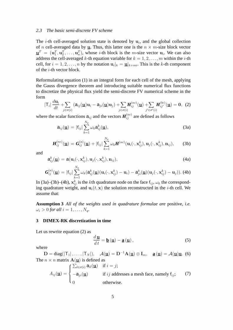
inclination angles and thus forms well-known shock patterns at the final integra-tion time. As we are only interested in measuring the CPU times for the variousDIMEX-RK schemes, a detailed analysis of these shock interaction phenomena isbeyond the scope of this paper. Thus, we refer the reader to Reference [11] andthe bibliography therein for a thorough description of thismodel problems. We listbelow the major simulation parameters that characterize each test case. We alsoprovide for each test case a figure that shows the approximatesolution at the finaltime step as indicated below. The approximate solution shown in each figure is cal-culated by using the a piece-wise linear reconstruction, the HLLE numerical fluxand the ERK(2) time integrator.

(i) Single Mach Reflection:Mach numberMs = 2.03, compression angle270, mesh of59756 triangles, finaltime t = 100µs, solution shown in Figure 1;

(ii) Complex Mach Reflection:Mach numberMs = 10.37, compression angle100, mesh of34833 triangles,final timet = 20µs, solution shown in Figure 3;

(iii) Double Mach Reflection:Mach numberMs = 8.7, compression angle270, mesh of49179 triangles, finaltime t = 24µs, solution shown in Figure 2.

For a complete description of the model problem and the threetest cases, we referthe reader to Reference [11] and the bibliography therein.

Table 5 illustrates the performance of the schemes ERK(2) and DIMEXMDP(1,2,2). Row#Iter reports the total number of iterations required to solvethe non-linear algebraic system (9) by applying the iterative procedure of equa-tion (12). The non-linear solving procedure implements a standard Richardson iter-ative scheme [15] coupled with an incompleteLU preconditioner [16]. RowsRec.,Chem.andSteprespectively detail the computational time (in seconds) needed toperform second order reconstructions, the update of the chemical terms, and therest of the integration time-step. Finally, RowTot. Timegives the total CPU timeto perform the run, and Row% Gain the percentage gain obtained by using theDIMEX-RK scheme instead of the explicit one.

Let us remark that the reconstruction procedure, which is needed to attain secondorder accuracy in space, is the same for both ERK(2) and MDP(1,2,2) methods andmust be performed at each time-step. The reconstruction is an important entry inthe overall computational costs, but its impact is less dramatic in the DIMEX-RKcase than in the explicit one. This is because the former scheme allows a greatertime step size and requires less time iterations to perform the same calculation.The update of the chemical terms (RowChem.) and the rest of the integration timestep (RowStep) is less expensive for the explicit scheme, because the DIMEX-RK method requires the iterative re-solution of a set non-linear algebraic systems.Nonetheless, from the viewpoint of global computational costs (RowTot. Time) the

15

−0.0100.020.040.060.080

0.01

0.02

0.03

0.04

0.05

0.06

0.07

0.08

1.011.5

2

2.5

3

3

3

3.4

3.4

3.4

3.4

3.41

3.41

3.41

3.41

3.49

3.49

3.49

3.49

3.57

3.57

3.57

3.57

3.65

3.65

3.65

3.65

3.733.73

3.8

3.88

Fig. 1. Single Mach Reflection atT = 100µs

00.010.020.030.040.050.060.070

0.01

0.02

0.03

0.04

0.05

5

6.82

10

10

10

10.6

10.6

10.6

12.5

12.5

13.2

13.213.2

13.8

13.8

13.8

14.4

14.4

14.4

15

15

15

15.7

15.7

16.3

16.3

16.9

16.9

16.9

17.6

17.6

17.6

18.2

18.2

18.2

18.8

18.8

19.4

19.4

20.120.7

21.3

22

Fig. 2. Double Mach Reflection atT = 20µs

DIMEX-RK method is always more efficient. The percentage gain (Row% Gain)is in the range[30, 60]%.

16

00.010.020.030.040.050.060.070

0.01

0.02

0.03

0.04

2

46

8.72

8.73

9.11

9.11

9.11

9.67

9.67

9.67

10.6

10.6

10.6

11

11

11

11.4

11.4

11.4

11.8

11.8

11.8

12.2

12.2

12.6

12.6

13

13

13.3

13.3

13.7

13.7

14.1

14.1

Fig. 3. Complex Mach Reflection atT = 24µs

Table 5Perfomance of ERK(2) and MDP(1,2,2) schemes on a 2-D reactive compressible flow cal-culation; the CPU times are in seconds.

Problem SINGLE COMPLEX DOUBLE

Method ERK(2) MDP ERK(2) MDP ERK(2) MDP

#Iter. 1626 771 1512 455 1753 524

Rec. (sec) 3400 1590 1850 556 3040 910

Chem.(sec) — — 318 565 513 852

Step (sec) 5980 5360 3650 2540 5990 4130

Tot. Time (sec) 9370 6960 5810 3660 9540 5900

% Gain 35% 59% 61%

7 Conclusions

In this paper, we studied some theoretical properties of theDIMEX-RK FV integra-tors that have been developed for multi-dimensional hyperbolic systems in [1]. Wedemonstrated that this approach produces a time evolution matrix operator whichshows a peculiar block structure common to a wide family of numerical fluxes. Theunderlying block matrices are M-matrices and the analysis which can be carried onwithin this context allowed to show that simple and efficientresolution algorithmseven for high-order schemes can be built. Although this FV scheme has been de-veloped for unstructured mesh calculations all the theoretical results proved herecan be straightforwardly extended to schemes defined on structured cartesian orcurvilinear meshes.

Finally, the performance of the method has been experimentally investigated. A setof representative time integration schemes up to third order global accuracy appliedto a 1-D test case has been considered to measure the approximation accuracy ofthe method. The computational efficiency of the DIMEX-RK approach when com-pared to an explicit integration time stepping scheme has been measured on a morecomplex application concerning with the simulation of a 2-Dreactive compressible

17

flow. All these experimental investigations illustrate that this approach performs ingood accord with the theoretical predictions.

Acknowledgments

The authors are grateful to Prof. T. Ruggeri and Prof. G. Russo for their usefulsuggestions.

References

[1] E. Bertolazzi, G. Manzini, Diagonally Implicit–Explicit Runge Kutta methods formultidimensional hyperbolic systems. Part I: Formulationof the method, (submitted).

[2] P. G. Ciarlet, The finite element method for elliptic problems, North-HollandPublishing Company, Amsterdam, Holland, 1980.

[3] E. Bertolazzi, G. Manzini, Algorithm 817 P2MESH: generic object-oriented interfacebetween 2-D unstructured meshes and FEM/FVM-based PDE solvers, ACM TOMS28 (1) (2002) 101–132.

[4] P. R. Halmos, Finite-Dimensional Vector Spaces, Van Nostrand, Princeton, N.J., 1958.

[5] U. M. Ascher, S. J. Ruuth, R. J. Spiteri, Implicit-explicit Runge-Kutta methods fortime-dependent partial differential equations, Appl. Numer. Math. 25 (2-3) (1997)151–167, special issue on time integration (Amsterdam, 1996).

[6] L. Pareschi, G. Russo, Implicit-Explicit Runge-Kutta methods and applications tohyperbolic systems with relaxation, J. Sci. Comp.To appear.

[7] O. Axelsson, Iterative solution methods, Cambridge University Press, Cambridge,1994.

[8] A. Berman, R. J. Plemmons, Nonnegative Matrices in the Mathematical Sciences,SIAM, Philadelphia, 1994, (republished in “Classics in Applied Mathematics”).

[9] R. S. Varga, On diagonal dominance arguments for bounding ‖ A−1 ‖∞, LinearAlgebra and Appl. 14 (3) (1976) 211–217.

[10] E. Zeidler, Nonlinear Functional Analysis and its Applications, Springer-Verlag, NewYork, 1986.

[11] E. Bertolazzi, G. Manzini, A triangle-based unstructured finite volume method forchemically reactive hypersonic flows, J. Comput. Phys. 166 (2001) 84–115.

[12] Z. Horvath, Positivity of Runge-Kutta and diagonally split Runge-Kutta methods,Appl. Numer. Math. 28 (1998) 309–326.

[13] S. F. Liotta, V. Romano, G. Russo, Central schemes for balance laws of relaxationtype, SIAM J. Numer. Anal. 38 (4) (2000) 1337–1356 (electronic).

[14] A. Kurganov, E. Tadmor, New high-resolution central schemes for nonlinearconservation laws and convection-diffusion equations, J.Comput. Phys. 160 (1) (2000)241–282.

[15] R. S. Varga, Matrix iterative analysis, expanded Edition, Springer-Verlag, Berlin,2000.

18

[16] G. H. Golub, C. F. Van Loan, Matrix computations, 3rd Edition, Johns HopkinsUniversity Press, Baltimore, MD, 1996.

19