IRLE

IRLE WORKING PAPER#156-07

June 2007

Trond Petersen, Andrew Penner, and Geir Hogsnes

The Motherhood Wage Penalty: Sorting Versus Differential Pay

Cite as: Trond Petersen, Andrew Penner, and Geir Hogsnes. (2007). “The Motherhood Wage Penalty: Sorting Versus Differential Pay.” IRLE Working Paper No. 156-07. http://irle.berkeley.edu/workingpapers/156-07.pdf

irle.berkeley.edu/workingpapers

The Motherhood Wage Penalty: Sorting Versus Differential Pay

Trond PetersenAndrew PennerGeir Høgsnes

University of California, Berkeley and University of OsloUniversity of California, Berkeley

University of Oslo

June 01, 2007 (First Version)

∗Portions of this paper will be presented at the annual meeting of the American SociologicalAssociation in New York City in August 2007, and has been presented at seminars atStanford University, MIT, Harvard University, Yale University, and University of California,Berkeley. Several meeting and seminar partipants made useful comments for which we arethankful. Trond Petersen is grateful for financial support from the Upjohn Institute andfrom the Institute of Industrial Relations at the University of California, Berkeley.

Address for correspondence: Trond Petersen, Professor, Department of Sociology, 410 Bar-rows Hall, University of California, Berkeley. Berkeley, CA 94720–1980, USA. Tel.: 1–510–642–6423. FAX: 1–510–642–0659. E-mail: trond@haas.berkeley.edu.

Andrew Penner, PhD Candidate, Department of Sociology, 410 Barrows Hall, Universi-ty of California, Berkeley. Berkeley, CA 94720–1980. USA. Tel.: 1–510–708–7465. E-mail:penner@berkeley.edu.

Geir Høgsnes, Professor and Chair, Department of Sociology and Human Geography, Uni-versity of Oslo. P. O. Box 1096 — Blindern. 0317 Oslo. Norway. Tel.: 47–22–85–42–61.E-mail: geir.hogsnes@sosiologi.uio.no.

Title

The Motherhood Wage Penalty: Sorting Versus Differential Pay

Abstract

The motherhood wage penalty is today probably the largest obstacle to progress

in gender equality at work. Using matched employer-employee data from Norway

(1980–97), a country with public policies that promote combining family and career,

we investigate (a) whether the penalty arises from differential pay by employers or

from sorting of employees on occupations and establishments, and (b) changes in the

penalties over time in a period with major changes in family policies. The findings

are as follows. (1) There are major wage penalties to motherhood, but these declined

strongly over the 18–year period, likely caused by changes in family policies and

in how families operate. (2) The penalty to motherhood is mostly due to sorting

on occupations and occupation-establishment units. By 1995–97, mothers and non-

mothers working in the same occupation-establishment unit were paid same wages.

(3) Women who become mothers are wage wise positively selected, but the premia

are wiped out by the negative effects of actual motherhood. (4) For wage growth,

there were premia to motherhood in 1980–89, but none by 1990–97. In conclusion,

the motherhood penalty is not due to employers paying mothers lower wages and its

size appears sensitive to changes in family policies, with large reductions in penalties

over time.

1 Introduction

The movement for gender equality in the workplace addressed equal pay for equal

work, equality in hiring and promotion, and in some countries equal pay for work of

equal value. By the end of the twentieth century it was widely recognized that while

major progress has been made in the first two of those three domains, significant

obstacles to further progress arises today from a different source: the processes that

occur in the family and their interrelationships with work. There is a sense of a

serious roadblock, even a stalled revolution.

For men, marriage and to some extent children have positive effects on wages

and careers. For women, the opposite is the case, there are small differentials for

marital status but large penalties for having children. As the economic historian Eric

Hobsbawm (2000, p. 136) reflects in a retrospective on the twentieth century: “There

can be no doubt that the emancipation of women has been one of the great historical

events of the twentieth century. The problem for the twenty-first is to establish what

still has to be done, and what will probably happen.” He continues (p. 136): “There is,

however, a serious problem, and it has become increasingly serious: the extraordinary

difficulties for women of combining high professional posts with being mothers.”

Two key questions concerning this stalled revolution arise. Did it get stalled by

employers, through differential treatment, possibly favoring married men and fat-

hers, while discriminating against mothers? Or was it stalled by women and men

from the adaptations they make between the family sphere and work, from diffe-

rential household-division of labor and preferences for different lifestyles? This paper

explores competing explanations for the most significant part of this puzzle: the mot-

herhood wage penalty as well as the female marital premium. We address the role of

employer discrimination against mothers and the extent to which the penalties can

be ameliorated by family policies.1

Three central hypotheses have been put forth to explain the penalty to mother-

hood and the bonus to marriage (Chiodo and Owyang 2003; Budig and England

2001, p. 204): The selection, treatment, and discrimination hypotheses.

The selection hypothesis argues that women who have children are less productive

than women who don’t, sometimes referred to as the unobserved heterogeneity hy-

pothesis. The treatment hypothesis proposes that upon parenthood women become

less productive: from lower work effort and/or loss of human capital accumulation.

The discrimination hypothesis claims that employers treat women with children dif-

1A separate paper addresses the male marital and parenthood premia, which have differentstructures, and probably different causes. Many of the issues are similar, but given the differentempirical patterns and complexity of results, separating the findings facilitates their presentation.

1

ferently, due to taste and/or statistical discrimination and even nonconscious biases.

These processes and their effects are however amenable to change. Large-scale

cultural transformations over the last 30 years have certainly affected family values

and work-family priorities. A central goal of the women’s movement was to change

how families operate, by having men do more work in the home and more caring

for children, thereby hopefully freeing up time for women to be active on an equal

footing with men in the marketplace. But employers too have been affected by the

cultural changes, and are probably more willing today to accomodate constraints

arising from family obligations than 30 years ago. The processes can also be changed

through family policies, many of which aim at facilitating combining family and

career. These can shift the incentives and the feasibility for being active in market

work for women, and hence also the bargains that are struck within the family.

Against this background we address several issues. The first objective is to assess

the extent to which the motherhood penalty (and secondarily the marriage premium)

arises from differential treatment by employers: (a) whether employers pay women

differently according to motherhood and marital status, (b) the role of sorting of

employees on occupations and establishments for the size of penalties (and premia),

and (c) whether the penalties (and premia) are due to promotion and wage growth

differentials. We cannot address discrimination in hiring, but we can assess the role

of pay and promotion penalties to motherhood, two important aspects of potential

differential treatment in the workplace. The second objective is to assess how these

penalties have evolved over time during a period when significant family policies have

been unrolled. To this end we use matched employer-employee data from Norway in

the period 1980–1997. Our data enable us to provide entirely novel and crucial em-

pirical angles, by documenting where the penalties arise, at the level of the employer

in how they pay and promote mothers and non-mothers, or in how employees are

sorted on establishments and occupations. The longitudinal aspect of the data allows

us to investigate the change over time in the penalties.

Why are these questions important? They are important because if the roadblocks

arise at the level of employers, or fail to arise there, then there are significant public

policy implications. Employers are easier to regulate than families, and if gains can

be had by further regulation of employers, then this should be done. If employers are

not a culprit, an increased emphasis on family policies is warranted. The question

then arises as to whether such policies have had effects in settings where they have

been tried on a large scale. Nowhere have family policies been more extensive than

in Scandinavia. Major policies to reinvent the family were rolled out over the last

20–30 years. But have they worked? Have they led to one of their goals, to facilitate

2

employment and careers for mothers? Scandinavia, including Norway, may now be

the place where the revolution is unstalling.

The national setting is thus significant and of broad interest. Scandinavia along

with the U.S. are in the forefront in regards to gender equality policies and both have

progressive values toward gender equality. The U.S. led the world in regulation of the

workplace, being the first country to pass extensive equality legislation. Scandinavia

is the vanguard in family policies, having adapted policies often identified as central

(Waldfogel 1998, pp. 141–145; Dex and Joshi 1999, pp. 655–656): paid parental leave

with a portion reserved for fathers, cash and tax benefits for children, publicly provi-

ded child care at high quality and low cost, and employment policies allowing flexible

hours and practically universal access to part-time work. While most Scandinavian

family policies are gender neutral, their first-order impact is primarily on mothers,

making it easier to combine family and careers, where female labor-force participa-

tion rates now are close to male rates, though with higher rates of part-time work

for women. The second-order impact is however on the adjustments fathers make. In

passing Norwegian family legislation an explicit goal expressed during parliamentary

debates was to redefine the family institution, by shifting the culture around how

families operate. We thus provide evidence on the motherhood penalty in a country

where public policy has done much first to make it easier to combine family and ca-

reer and second to change the internal organization of the family by trying to create

a more equal division of household labor between the sexes, with internationally now

one of the most equal such divisions (Hook 2006, Fig. 1, p. 650).

A caveat is in order. Ultimately it is probably impossible to discern the precise

effects of family policies on the motherhood penalty, simply because policies work

out over many years and come bundled with other changes. Policies impact fertility,

the work-family interface, and employer adaptations, each of which adjusts slowly

over several years. But then there have been concurrent changes in family culture

and decline in discrimination against women more generally. Empirically one thus

faces an entire constellation of changes. But to the extent that declines have occurred

in the motherhood penalty over the last 20–30 years, family policies likely have been

a major contributing cause.

2 Selection, Treatment, and Discrimination

In four subsections we review the three hypotheses (2.1), discuss our core errand,

the role of differential pay within versus sorting on establishments, occupations,

and occupation-establishment units for how the penalties arise (2.2), summarize the

3

implications of the hypotheses (2.3), and summarize existing evidence (2.4).

2.1 Women and Family

Three central hypotheses have been put forth to explain the motherhood penalty and

the female marital premium (Chiodo and Owyang 2003; Budig and England 2001, p.

204). Since the marital premium is modest for women, but the motherhood penalty

is substantial, the focus will be on the mechanisms behind the latter.

The selection hypothesis works best for the marital premium. The factors that

cause married women to earn more are the same factors that cause them to get marri-

ed: conscientiousness, industriousness, and other traits valued both by employers and

prospective partners.2 Marriage as such does nothing to increase their productivity.

But women who get married also tend to get children, and there is a clear children

penalty. The selection hypothesis may explain the marital wage premium, but not,

without further elaboration, the children penalty. For the latter, it may be that less

productive women tend to have children at younger ages, in which case the penalty

in part is a selection effect (Taniguchi 1999; Amuedo-Dorantes and Kimmel 2005).

Several implications follow from this hypothesis. To the extent that productivity

can be observed and hence rewarded by employers, there should be no wage diffe-

rences at the individual level of getting married or having children: as individuals

move between marital and motherhood statuses, there should be no wage changes.

This also means that women who eventually marry or have children even prior to

entrance into marriage or motherhood earn a wage premium or penalty relative to

women who remain single and childless.

According to the treatment hypothesis, getting married and having children in-

duce women to change their behavior. Productivity goes up with marriage and down

with children. Two mechanisms that could produce this result have been put forth.

One mechanism posits that mothers exert less effort at work than non-mothers.

This could arise simply from the time constraints children give rise to, even when mot-

hers and fathers share equally in householdwork and in taking care of children. But

with household specialization this effect gets excacerbated, with further reduction of

effort in the market for women, while often the opposite for men (Becker 1985). The

lower effort in market work can occur in the same workplace, possibly leading to a

wage penalty in the same job. It can also occur through changing to less demanding

workplaces, in which case the children penalty manifests itself not at the workpla-

2Mueller and Plug (2006) report wage bonuses for a variety of personality traits which may ormay not be related to productivity, for example, that men are rewarded for being antagonistic,while women for opennes to experience.

4

ce level, but in occupational segregation. The policy implications to be drawn with

respect to removing the motherhood penalty varies by the source of lower effort.

If there is equal distribution of work in the household, and the only added burden

is having children, better family-work policies are needed, for example, by provi-

ding high-quality child care at low cost. If there additionally is unequal distribution

of work within the family, one need also to change how families operate, through

cultural campaigns, perhaps the tax system, and more.

A second mechanism in the treatment hypothesis points to less human capital

accumulation during marriage and motherhood. There is loss of experience and on-

the-job training as a result of part-time work and career breaks.

Under both mechanisms the motherhood penalty should have declined over time,

in part because public provision of child care has increased and in part because the

household division of labor and caring for children have become more equal, providing

women with more time for market work today than earlier. For example, in the U.S.,

average household work for married mothers decreased from 34.5 to 19.4 hours per

week between 1965 and 2000, while among married fathers it increased from 4.4 to

9.7 hours, an increase in the share done by men from 13 to 33% (Bianchi, Milkie,

Robinson, and Milkie 2006, p. 93, Table 5.1).

The discrimination hypothesis, in contrast, does not rest on the claim that mot-

hers are less productive than non-mothers, at least not in its pure form. It argues

that employers discriminate against mothers. In its pure form the hypothesis puts

forth that the differential treatment arises from animus (or taste) discrimination,

where an employer has a distaste for working mothers, comparable to when an em-

ployer is willing to pay more for certain demographic groups, such as hiring more

from and paying more for white than black employees, even in absence of objective

reasons for doing so (England 1992, chap. 3). In a less pure form, mothers may in

fact on average be less productive than childless women—be it due to selection or

treatment—but without each mother being less productive than each childless wo-

man, net of other characteristics (Hill 1979, p. 592). When productivity is costly to

observe and measure, employers may act as if the group average applies to each group

member, and will pay more for childless women than for mothers. It would be an

instance of statistical discrimination (England 1992, chap. 3), and would, if costs of

measuring productivity are high, be economically rational behavior. This relates to

an older historical phenomenon. Before and at the turn of the twentieth century, and

especially up through the 1920s and 1930s, many organizations practiced a so-called

marriage bar, under which married women were not hired and women upon marriage

5

or childbirth often were fired.3 Additionally there may be nonconscious sources of

discrimination, as stressed in much recent psychological, legal, and sociological scho-

larship (e.g., Greenwald and Krieger 2006), with same effects as the conscious taste

and statistical discrimination.

While these three hypotheses typically are used to explain the relationship betwe-

en family and wages for both men and women, it needs to be added that the issues

for women are considerably more complex. They involve a set of sequential decisions

made under significant uncertainty and partial knowledge about future personal, or-

ganizational, and societal conditions, such as timing of pregnancy, duration of career

breaks, public policy, and more. But a tractable analysis needs to set more limited

goals than analyzing the entire set of life-cycle decisions.

2.2 The Role of Sorting

Regardless of the precise mechanisms producing the children penalties (and secon-

darily the marital premia), it is instructive to ask, Where do these penalties arise?

Do they arise at the level of employers, when mothers and non-mothers work in sa-

me occupation and establishment? Or do they arise in the sorting of employees on

occupations and establishments, so that non-mothers are hired and promoted into

the higher-paying establishments, occupations, and occupation-establishment units?

And if the penalties arise due to sorting, does the sorting come from employee

choice in which establishments and occupations to work in, or does it come from

employer choices favoring childless women over mothers? A subtle implication ari-

ses here that allows us to gain some insight into the role of employee choices and

productivity versus employer discrimination. If the women who eventually get mar-

ried and have children, while they still are single and childless, sort into the better-

or lower-paying occupations and occupation-establishment units to a higher degree

than the women who remain single and childless, then some of the sorting must occur

due to choice or assessed productivity. The reason is simply that employers have no

opportunity among single and childless women to discriminate on the basis of their

future marital and motherhood status, and if sorting still occurs, it is unrelated to

employer preferences for single over married women or childless women over mothers,

and thus not caused by discrimination.

3For the U.S. see Goldin (1991) and for Norway see Hagemann (1994).

6

2.3 Summary of Main Implications

It is useful to summarize the main empirical implications of the hypotheses. All three

hypotheses agree that mothers suffer a wage penalty relative to non-mothers. They

differ in the mechanisms proposed for the penalty.

According to the selection hypothesis, more relevant for the marital premium

than for the motherhood penalty, the women who eventually marry will earn high

wages also prior to marriage, will not increase their wages upon marriage, and will

not decrease wages upon separation, divorce, or widowhood. Women who become

mothers will suffer a wage penalty also prior to entrance into motherhood.

According to the treatment hypothesis, women who are mothers suffer a wage

penalty relative to non-mothers, simply because of their decreased effort in market

work upon motherhood, either in same occupation in same workplace or through

change of occupation and workplace. Over time there will also be loss in human

capital accumulation which induces additional penalties.

In the discrimination hypothesis, there will be low wages induced from being

a mother, regardless of whether this is due to animus against working mothers or

statistical discrimination. Under statistical discrimination, however, as mothers gain

seniority with the same employer, productivity gets revealed and high-productivity

mothers may be rewarded accordingly and no longer as being representative of the

average mothers.

Two of the hypotheses also have specific implications for the historical trend

in the penalties. Both the treatment hypothesis and the animus mechanism under

the discrimination hypothesis would imply a decline in penalties over time, as the

distribution of household work has become more equal, with less loss in human

capital accumulation, and the amount of animus against working mothers probably

has declined.

Additionally, according to the selection hypothesis, to the extent that the pre-

mium arises from sorting rather than from differential pay for same work for same

employer, and this sorting is due to employee choices or to observable productivity,

we should observe that the sorting occurs even prior to marriage and motherhood.

This would be evidence against discrimination from employers based on animus.

The procesess implied by the three hypotheses also interact. For example, as the

household division of labor has become more equal over time, some employers will

observe that some mothers have more time or effort left for market work, which in

turn may lead them to revise their statistical estimates and perhaps engage less in

statistical discrimination.

In summary, we have three separate hypotheses, and the second and third each

7

has two separate mechanisms, producing different outcomes at different levels. This

can become intricate, and to focus ideas Table 1 summarizes the implications.

(Table 1 about here)

2.4 Summary of Research Evidence

Since our empirical aims are different from what has been addressed by research to

date, only the central findings are discussed below. We start with the U.S. evidence.

With respect to marriage, Waldfogel (1997) in a cross-sectional analysis finds a

positive effect of about 6%, which goes down to 4% with controls for individual-level

fixed effects. Hundley (2000) reports non-significant marital wage differentials from

–2.0 to +3.0% for employed women in one data set but significant premia of 5–8%

in another data set. Studies using earlier data find similar results, marital premia of

1–5% in Korenman and Neumark (1992), of 3.6–4.8% in Hersch (1991), and of 4.2

and 6.7% for white and black women respectivel in Hill (1979).

For children, Waldfogel (1997) reports cross-sectional penalties of 4 and 9.6% for

1 and 2+ children, and even larger within-individual penalties of 5.6 and 14.7%, from

comparing an individual’s wages before and after motherhood. Budig and England

(2001) report similar penalties: in cross-sectional analysis of 3.9, 7.1, and 5.3% for

1, 2, and 3+ children, which increase to 4.5, 11.2, and 15.1% in within-individual

analyses. Anderson, Binder, and Krause (2003) show cross-sectional penalties of 5–

9% and 7–13% of 1 and 2+ children, but these drop to 3 and 5.5% in within-individual

analyses, with somewhat larger penalties in Anderson, Binder, and Krause (2002).

Amuedo-Dorantes and Kimmel (2005) find cross-sectional penalties of 4.5 and 8.8%

for 1 and 2+ children, which increase to 4.9 and 10.3% in within-individual analyses.

Hundley (2000) reports wage penalties of 8, 15, and 23% for 1, 2, and 3+ children,

and substantially larger children penalties among self employed women. But from

another data set, he shows no penalties to 1 and 2 children but a 6% penalty for

3+ children. Lundberg and Rose (2000) find that women who stay continuously

employed after childbirth suffer no wage penalties whereas women who take career

breaks suffer a 5% wage penalty. Taniguchi (1999) finds smaller children penalties

for women who delay childbirth and Amuedo-Dorantes and Kimmel (2005) even find

children bonuses among the highly-educated women who do so.

As for earlier studies, Korenman and Neumark (1992) report penalties of about

15% for 2+ children in both cross-sectional and within-individual analyses. From

more complex econometric analyses they conclude that with continuous employment

there is no children penalty. Hill (1979) finds a 6.9% penalty per child 18 years or

8

younger among white women, but no penalty for children among black women.

Two studies do find positive effects of children. From a sample of 217 women

employed in 18 firms Hersch (1991) find premia of 2.8–4.1% per child, while Hersch

and Stratton (1997) report positive effects of up to 4 younger children. The small

sample size in the first study limits its generality.

Regarding the role of household specialization Hersch and Stratton (2002) find

that both married and unmarried women suffer a wage penalty from housework,

among married women of about 4% for a ten hour increase in weekly housework

hours. The penalty is incurred when they perform typically female tasks in the hou-

sehold, but not for male or sex neutral tasks. Hersch and Stratton (1997) report a

negative effect of housework hours: wages decrease with 5.5% for a 10 hour increase

in housework, but with a very small effect of housework hours once within-individual

analyses are done.

On balance, the studies show relatively small marital premia of 4–6%, but sub-

stantial children penalties, up to 15–20% for 2 or 3+ children. Three of the studies

show large penalties within women’s lives as they transition between having 1, 2,

and 3+ children, larger than the penalties found between mothers and non-mothers

in the cross section. This suggests major treatment effects on wages for women.

Several comparative studies investigate marital premia and children penalties and

some studies address these specifically in the Scandinavian context, though research

on Norway is limited.

With respect to marriage, Harkness and Waldfogel (2003) find premia of 2 and

3% in Finland and Sweden, while Albrect, Edin, Sundstrom, and Vroman (1999)

report premia in Sweden of about 1%. Isacsson (2006) in large-scale longitudinal

study of Swedish twins, finds that among identical twins there is 11% marital wage

penalty, which gets reduced to 7.2% when within-twin analysis is conducted, and to

0.5% and non-significance when within-individual analysis is done. This analysis did

not include controls for children.

Harkness and Waldfogel (2003) report the largest children penalties in the U.S.,

UK, and Germany, and the lowest in the Nordic countries. The country-specific

Scandinavian studies report small penalties to motherhood. For Denmark they are

1% for 1 child and 2% for 2+ children in cross-sectional analysis, but when within-

individual analyses are done, then there are even small positive effects of having

children of less than 0.5%, controlling for other variables, but effects that do not reach

statistical significance (Datta Gupta and Smith 2002, Table 2, p. 618). Using the same

data, Nielsen, Simonsen, and Verner (2004) refine these findings. They demonstrate

that in the family-friendly public sector of the economy there are negative effects

9

of being a mother, a penalty of about 2.4%, but that in the private sector there

are no such effects, a non-significant penalty of about 0.7%. They also investigate

whether women upon childbirth self-select into the public sector. For example, 52%

of women employed in the private sector have no children, while this is the case

for only 38.5% of those in the public sector (Table 1, p. 727). Rosholm and Smith

(1996) find similarly small effects of motherhood in Denmark in 1980–1990. Davies

and Pierre (2005) report children penalties in Denmark, of 0, 3, and 3% for 1, 2, and

3+ children, but then substantially larger penalties in within-individual analyses of

3, 8, and 13%. Albrecht, Edin, Sundstrom, and Vroman (1999) report similar types

of analyses for Sweden, finding that women are penalized neither in the public nor

private sector for taking maternity leave. As in Denmark, there is, after controlling for

career interruptions, even a premium for having children among the highly educated.

The single study of Norway does however find wage penalties to motherhood, but

no within-individual analysis is reported. As in the Danish study, the penalties are

higher in the private than public sector (Hardoy and Schøne 2004).

The evidence is clear that Denmark and Sweden have lower marital premia and

lower children penalties than the U.S. Norway has yet to be studied in detail.

Regardless of country, no study has used matched employer-employee data to

analyze the premia and penalties. These are required for ascertaining whether there

is different pay for the same work for the same employer, that is, whether productivity

differences and/or discrimination could have arisen at that level. Nor has any study

addressed the role of sorting on occupations and occupation-establishment units.

And there is no documentation of the evolution of the premia and penalties over

time, of the extent to which they have changed as family policies have been unrolled.

3 Setting and Data

National Setting

Norwegian family policies have been considerably more elaborate than in most other

countries, though not at the level of Swedish policies. They include paid parental

leave, with some portion reserved for fathers, so as to strengthen the bond between

fathers and children and thereby creating entirely new norms for fatherhood (Leira

2002, chap. 4). They include tax and cash benefits for families with children. Most

important, there is publicly supported child care at relatively low cost and high

quality. Additionally, part-time and work at flexible hours are almost universally

available, and with no wage penalty to being part-time employed. These are all

institutional arrangements central to lessening the family gap in pay and careers

10

(Waldfogel 1998).

With respect to parental leave, it was available for 18, 20, 22 weeks in 1977, 1987,

and 1988, with 100% pay since 1978. Since 1977 fathers could share the leave except

for the first six weeks which were reserved for the mother. Between 1988 and 1993,

parental leave was increased with a few weeks every year from 22 to 52 weeks at 80%

pay or for 42 weeks at 100% pay up to a maximum amount (Rønsen and Sundstrom

2002). Four of those weeks are reserved for the father, whereas six weeks are reserved

for the mother (Leira 2002, pp. 89, 95). In 1996, 69% of fathers took paid parental

leave and about 7% of the parental leave days (Leira 2002, pp. 86, 91).

With respect to child care, 5% of preschoolers had access to publicly funded child

care in 1973, 25% in 1983, and 32% in 1988. By 1995, 22% of 0–3 and 61% of 3–6

year olds attended publicly supported child care (Leira 2002, p. 62). Single parents

pay lower fees. The cost of child care as percent of female earnings is 13 in Norway,

while an entire 22 in the US (Waldfogel 1998, Table 2).4

While the policies on average impact women more than men, by making it easier

to combine family and career, their impact on how both members of a couple behave

can be substantial. With mothers more likely to be employed, and with cultural pres-

sures on fathers to become more involved in household activities, the gender division

of labor in the household is likely to be more egalitarian than in other countries. This

further facilitates career success for mothers through getting more help from men in

running the household and caring for children. Internationally, Norway—along with

Sweden, Canada and the U.S.—has one of the most equal divisions of household

labor (Hook 2006, Fig. 1, p. 650), and along with Sweden scores at the top of the

Gender Empowerment Measure of the Human Development Report (United Nations

Development Program 1998).

Data

We use matched employee-employer data on entire populations of white-collar em-

ployees in central sectors of the Norwegian economy in the period 1980–97. These

allow us (1) to compare employees working in the same occupation for the same

employer, and to make those comparisons between single, married, previously mar-

ried, and those with and without children, (2) to assess the role of sorting, and (3)

to analyze wage growth and promotions between years. Information is available on

about 110,000 employees (about 40,000 women from 1990 on) and 3,000 establish-

4Esping-Andersen (1999, p. 66, Table 4.4) in contrast argues and documents that net costs forchild care in the U.S. are among the lowest internationally, stating that even in the absence ofpublicly provided child care “the United States offers a superior cost-subsidy mix”; as a percent offamily income with costs equal to those in Denmark and France and lower than in Sweden.

11

ments each year. We can follow establishments and their employees from year-to-year,

about 800,000 person-years for the women. We restrict the analysis to women 20–50

years old, leaving about 600,000 person-years. For each employee we have informa-

tion on sex, occupation, rank in occupational hierarchy, age, part- versus full-time

status, contractual hours worked, and monthly earnings from work on contracted

hours, which excludes wages on overtime hours. The data were matched to register

data from the Central Bureau of Statistics on education (length and type, 4 digit

code), family or civil status (8 statuses), number and ages of children and adoptions.

This gives annual educational, marital, and parental histories up to year 2000.

The data were collected from individual-level records kept by the establishments

and compiled by the Norwegian Central Bureau of Statistics and the main employer’s

association in Norway, the Confederation of Business and Employers (NHO). Norwe-

gian employers are bound by law to collect and report the data (e.g., Central Bureau

of Statistics 1991, pp. 120–123). They are used in wage bargaining and economic

planning and should be reliable compared to information from sample surveys with

personal reports of pay rates, hours worked, and occupation or position.5

These data on white-collar employees cover all occupational groups with a few

exceptions: CEOs, working supervisors, top editors of newspapers, secretary to the

editor of newspapers, and journalists. While working supervisors are excluded, su-

pervisors in administrative positions are included.

The data come from a variety of industries: manufacturing, oil extraction, mining,

quarrying, transportation, storage, communication, and other industries. Most of the

industries outside the manufacturing sector are relatively small, but the hotel and

research sectors count 2,201 and 4,771 employees respectively in 1990. This grouping

of industries is used by the Norwegian Central Bureau of Statistics. It is the first

sector to carry out wage negotiations and is thus central for wage setting in other

sectors, and is typical of other major sectors in the economy. For our purposes it is

a strategic sector. Of the seven sectors from which gender wage gaps were computed

for 1990, it had the largest gaps at all levels, also the occupation-establishment

level (Petersen, Snartland, Becken, and Olsen 1997). This ensures variation in the

dependent variable especially at the occupation-establishment level, which also could

show up in marital premia and parenthood penalties. The restriction of analyses to

these white-collar employees probably leads to results with somewhat larger penalties

than if additional employees had been included.

From the contractual monthly earnings and contractual hours worked we compu-

5The data are quite complete. For example, for the year 1992 we have complete data on 84% ofthe establishments and 94% of their white-collar employees.

12

ted the hourly wage, which then refers to hourly wages paid on regular work hours,

hence not mixing pay on regular and over-time hours. This is important since a cen-

tral goal of the analysis is to assess whether employers pay mothers and non-mothers

differently, in which case we need to measure the pay rate, not mixings the different

rates from regular and overtime hours. Five marital statuses are distinguished: sing-

le, married, separated, divorced, and widower. Among the married, separated, and

divorced, we include a few hundred employees in same-sex unions that were still in-

tact (“married”), ”separated”, and “divorced”; these are legal categories in Norway.

Including these cases does not affect the results. We coded three dummy variables for

number of children aged 20 or younger: for one, two, or three or more such children.

We experimented with a number of different codings for the children variables, such

as number of children below age 6, between 6 and 15, and so forth. The alternative

codings make no substantive difference for the conclusions arrived at in the analyses.

The occupational code is quite detailed, with 201, 210, and 209 occupations in

1980, 1990, and 1997. We use data on employees in 155 of these occupations, for

the simple reason that for those occupations a simple aggregation of 21 occupa-

tions exists, an aggregation which allows us to investigate promotions between years.

It makes no substantive difference for the results whether we use 21, 155, or 210

occupations. The gaps between groups are slightly reduced when more occupations

are used, but not the pattern of results. The coarser grouping of 21 occupations

also helps avoid the otherwise large loss of number of observations when computing

fixed-effects estimators at the occupation-establishment level. We need variation at

the occupation-establishment level not only in marital status, but also in whether

employees have 1, 2, or 3+ children aged 20 or younger.

Labor force experience is imputed as age minus 16, minus years of education

beyond age 16, minus one year per child. It makes no difference for results whether

we subtract a year per child or not.

Initially, we controlled for 21 educational groups, based on length and type. Our

final analysis uses a simplification with five educational groups, but with only small

differences in results. This choice followed from the same logic as when using only

21 occupational groups.6

In the promotion analysis we utilize the information on 21 occupational groups.

These are divided into five career ladders with respectively 9, 3, 5, 2, and 2 steps.

For employees who remain in same career ladder between two adjacent years, and

who are employed below the top step in the ladder, we can analyze promotions.

6Results using the full set of 155 or 210 occupations and the fuller set of 21 educational groupsare availabe from the authors upon request.

13

Table 2 provides descriptive statistics for our key variables, with annual averages

reported separately for each of four periods, 1980–84, 1985–89, 1990–94, and 1995–97.

Wages are 18–19% higher for married and previously married women compared to

single and childless women. Single women and childless women are however promoted

at higher rates, but no control is here made for labor force experience. On average

employees are observed for nine years.

(Table 2 about Here)

Our data suffer from one significant weakness. We do not know which women

are cohabitating. For the women who are recorded as single (i.e. not yet married),

some are truly single, others are cohabitating. Cohabitation is important in Norway,

increased over the period 1980–2000, and is more common in younger cohorts (Noack

2001). In 1990, about 58% of Norwegian women aged 20–66 were married and another

6% were cohabitating, with the remaining 36% being single. In our data, 26% percent

are recorded as single in 1995–97, but about one in six of the singles were probably

cohabitating, which would yield a correct percent single around 21. While we are not

aware of any Norwegian studies investigating wage premia for cohabitators, there are

such premia in Denmark of about 1% (Datta Gupta and Smith 2002).

Some biases arise from this misclassification, as documented by Cohen (2002) for

men using U.S. data. If cohabitators enjoy wage premia similar to married women,

the cross-sectional analysis will overestimate the wages of single women, while still

correctly estimating the wages of married women, and thus underestimating the wage

differential, that is, the marital premium. To the extent that cohabitating women are

more like single women in their economic success, there is no problem. In the within-

individual analysis some women will be misclassified as single while cohabitating,

and if there are treatment effects of leaving singlehood, a similar underestimation

occurs, but none if the entire premium is due to selection. Since the marital premium

for women is so small to begin with, about 2% (see below), the absolute size of the

bias will however be small. If one in three of single women are cohabitating, and they

earn the same premium as married women, the bias will be 1%: We will estimate the

marital premium to be 2% rather than the correct 3%.

4 Methods

The data have a unique multilevel structure. One level arises from the across-time

dimension, the other level, at a given time point, arises from the nesting of employ-

ees within occupations and establishments. Most individuals are observed at several

14

points in time, and some even every year in 1980–1997. This gives a standard panel

data set-up (e.g. Hsiao 1985; Petersen 2004). Similarily, each establishment is obser-

ved at several points in time, as much as every year in 1980–1997. In a given year,

we can account for the clustering of employees into establishments, occupations, and

occupation-establishment units, using standard fixed-effects procedures. Across years

we can exploit the panel-nature of the data, taking into account that some employees

are observed at more than one point in time, also using fixed-effects procedures, and

additionally we can account for the fact that some employees remain in the same

establishment, occupation, or occupation-establishment unit.

For each of three dependent variables, we report a sequence of four regression

equations. Each equation includes independent variables for education and imputed

labor force experience plus dummy variables for marital status and dummy variab-

les for the number of children below age 20. The first equation does not take into

account where the employees work nor their occupations, the second controls for

the establishment (workplace), the third for the occupation, and the fourth for the

occupation-establishment unit. The second, third and fourth specifications are esti-

mated using fixed-effects procedures. The four specifications will be referred as the

Population, Establishment, Occupation, and Occupation-Establishment estimators.

Each coefficient estimated is significantly different from zero usually at a high

level, often with z- or t-statistics of 40–50 and significance levels of .000001 or better.

No point is served in reporting these significance levels. The large z-statistics reflect

the large number of observations each year, not superior model specification.

The estimated equations and technical details are given in Appendix. Below we

give a verbal account.

Methods for Analyzing Total Effects on Wage Levels

The baseline analysis reports how wages depend on marital status and children,

controlling for education and imputed labor force experience, at each of the four

levels, population, establishment, occupation, and occupation-establishment. These

are referred to as total effects.

From the multilevel structure of the data we can assess how the employee outco-

mes within establishments and occupations differ from those occurring across establis-

hments and occupations. The estimates from the occupation-establishment analysis

will address whether the marital premia and parenthood penalties in wages are pre-

sent when same work is done for the same employer.

The equations are estimated separately for each of the 18 years in the data. This

allows us to assess possible changes over time, as implied by two of the hypotheses.

15

To simplify presentation, we report the averages of the coefficients within each of

four time periods, 1980–84, 1985–89, 1990–94, and 1995–97.

The dependent variable is the natural logarithm of the hourly wage. When small

(e.g., less than .10 in absolute value), a coefficient can be interpreted as giving the

relative change in the unlogged dependent variable from a one-unit increase in the

independent variable, holding the other variables constant. We implicitly interpret

this as the relative change in the mean of the unlogged wages, but correctly interpre-

ted it gives the absolute change in the mean of logarithms of wages or the relative

change in the geometric mean of unlogged wages (Joshi and Paci 1998, p. 160).

Accounting for Selection Effects

The analyses outlined above do not account for possible selection processes. Women

who have children may differ from those who do not in ways relevant for wages. The

next set of analyses therefore addresses this concern.

In a first analysis we selected only employees who in a given year are single and

childless. The variables for current marital and children status are then excluded.

But we introduce two new dummy variables, one for whether the employee some

time in the future got married and another for whether the employee eventually

had children, called “ever married” and “ever children”, each of them coded 1 for

employees who ever were married or ever had children during the period covered

in our data (up to 2000 for marital status and children), while 0 for everyone else.

Otherwise, the analysis is identical to the one described above. This provides an

estimate of the selection effect, whether future marital and parenthood statuses can

predict the wages while single and childless.

In a second variant we used information on all employees, but for the employees

who eventually got married and/or eventually had children, we introduced the same

two dummy variables for “ever married” and “ever children”, entered in each year the

employee was present in the data. In addition, as in the analyses of total effects, we

enter dummy variables for current marital status and current number of children. The

dummy variables for “ever married” and “ever children” estimate the selection effects

whereas the dummy variables for current marital and parenthood status estimate

treatment effects. The sum of the two dummy variables gives the total effect of

marriage and children, comparable to the analyses where we do not separate the

selection and treatment effects.

These two analyses address the question of selection effects most directly, asses-

sing whether these are present before entrance into the state of marriage or parent-

hood has occurred. The part of the marriage and children effects not due to selection

16

is then due to treatment, according to the interpretation given here.

Accounting for Treatment Effects

We estimate next the treatment effect more directly by utilizing the longitudinal

structure of the data. We add a fixed effect for the individual employee in addition

to fixed effects for establishment, occupation, and occupation-establishment. We then

assess whether individuals, as they transition between statuses—from single to mar-

ried to separated etc., and from childless to having 1, 2, or 3+ children—experience

within-individual changes in wages (premia or penalties) following such transitions.

We use the individual-level data from multiple years, observing employees before and

after family transitions.

Accounting for only individual or for only occupation-establishment fixed effects

is straightforward. Accounting for both at the same time is difficult. With two sets

of fixed effects there is no estimator where all the dummy variables “vanish” from

the estimation procedure. And with about 40,000 individuals each year, and so-

me 20,000 occupation-establishment units, estimating the effects of all the dummy

variables may be impossible. No computer software known to us can handle this.

Our solution was to adapt a simple procedure proposed by Goux, Dominique, and

Maurin (1999). We create an interaction term between the individual-level dum-

my variable and subsequently for the establishment, occupation, and occupation-

establishment dummy variables. This creates a fixed effect specific to the individual

and say the occupation-establishment unit in which she works. If the individual

changes occupation-establishment unit, a new dummy variable pertaining to that

individual and the new occupation-establishment unit is created.

This analysis addresses the question of treatment effects most directly, since it

estimates the effects at the individual level of getting married and becoming a parent.

As above, the part of the total effect not due to treatment, is then due to selection.

The two sets of analyses, of selection and treatment, may give somewhat different

results regarding their relative importance. When estimating selection effects, we

make comparisons to individuals who stayed single and childless. When estimating

treatment effects the comparison is intra individual, before and after the person

enters into marriage and parenthood.

A clarification of terminology should be noted. We uniquely can identify the

selection effect. But what we refer to as the treatment effect really consists of two

parts: The treatment effect, from possible employee adaptations to family situation,

plus the treatment effect of possible employer discrimination, from employers reacting

to changes in the family circumstances of their employees. These two cannot be

17

separated further with our data. But to the extent we find no penalties at one of

the levels, say the occupation-establishment level, then a reasonable inference is to

assume that there are neither true treatment nor discrimination effects at that level.

Methods for Analyzing Individual Career Dynamics

In addition to estimating wage differentials, we also analyze individual career dy-

namics. We first analyze changes in wages from one year to the next among those

employees who stayed in the sector in two adjacent years and remained in the sa-

me establishment, simply because we now primarily are concerned with what occurs

within firms. The dependent variable is the change in logarithm of wages from one

year to the next. The same set of models as for the wage levels are estimated.

Next we analyze promotions in occupational rank, for employees who remained

in (a) the sector between two adjacent years, (b) the same establishment, and (c)

the same career ladder, provided they had not reached the top of the ladder. Our

data allow us to investigate promotions within career ladders, where a hierachy of

occupations is defined, but not between ladders. In order to faciliate communication

of results, we estimate a linear probability model for promotion, where coefficients

can be interpreted directly as giving the difference in proportion promoted adjusting

for the other variables. Computationally it is also easier to estimate than a logit

model with fixed effects, given the large number of occupation-establishment units.

We report the same set of models as in the case of wage changes. The difference is

that the dependent variable now is binary, equal to 1 if a promotion occurred in two

adjacent years and equal to 0 if not.

How to Think About the Various Sets of Coefficients

How should one then think about the various estimates we report? A fruitful way

to think about the estimators is that they report on different aspects of the data,

that they answer different questions. The population-level estimator reports what on

average is the case when all individuals are compared, without making distinctions

about where they work and what type of work they do, both of which, in contrast,

are taken into account in the occupation-establishment estimator. It reports what

on average is the case at the occupation-establishment level. For example, one may

find in the population-level estimator that there is a positive effect on wages of

being married, whereas at the occupation-establishment level there is no such effect.

This would correctly indicate that married women earn higher wages than single

women, but that once employed—married or single—in the same occupation in the

same workplace, then there are no differences in wages. The reason for the premia in

18

the population-level estimator is that married women tend to work in higher-paying

occupation-establishment units than single women.

By comparing changes in coefficients as one goes from the population-level esti-

mator to the occupation- to the occupation-establishment-level estimators one will

be able to assess at what levels differences between groups arise: From differential

wages at say the occupation-establishment level, or from differential sorting of the

groups on occupations and occupation-establishment units.

Similarly, when we take into account individual-level fixed effects, then we assess

how transitions at the individual level from being single to married, from having

0 to 1 child, etc., on average impact the individual’s wages. We no longer make

comparisons between individuals, comparing say single to married, we rather make

comparisons of wages at the within-individual level between when they were single

and when they were married. Both types of comparisons are relevant to make, and

none is better than the other. They just address different questions, and we need to

focus on the estimator that best answers the corresponding question.

5 The Wage Gap By Marital Status and Children

Differential Pay Versus Sorting

Table 3 gives the coefficients on wages of marital status and number of children below

age 20. Each regression is estimated separately by year, for 18 years. But to make

presentation more compact, we have averaged the coefficients across years within

four separate periods: 1980–84, 1985–89, 1990–94, and 1995–97.

(Table 3 about here)

At the population level, with analyses comparable to results already reported in

the literature, the effect of marital status are similar across the four time periods:

Wages are 2% higher for married than single women, with a somewhat lower wage

bonus for previously married women. With controls for establishment, occupation,

and occupation-establishment these effects are cut in about half: The premia are

about 1% for being married and much smaller for post-marital states. The marital

premia are thus small, and close to zero at the occupation-establishment level.

The wage penalties for children are however substantial, especially in 1980–89.

In 1980–84 the penalties were 3.5, 7.6, and 10.7% for 1, 2, and 3+ children. But by

1990–97 the penalties were cut in half, to 2.3, 4.0, and 4.9% (in 1995–97).

As one successively controls for establishment, occupation, and the occupation-

establishment unit the penalties change. Controlling for establishment reduces the

19

children effects by a small 10%. But at the occupation-establishment level, the child-

ren effects are dramatically reduced with about 50% in 1980–89, about 75% in 1990–

95, and 90–100% in 1995–97: The penalties were 0.5–1.6% in 1990–95 and 0.1–0.5% in

1995–97, with almost as strong reductions at the occupation level. By the mid-1990s

the children penalties at the occupation-establishment level had thus disappeared,

and almost disappeared at the occupation level.

What can we then conclude? There are small premia for marital status, but

sizeable penalties for children. For women, as for men there is a premium to being

married, but it is much smaller than typical male premia (in Norway of 6–7%). For

women, unlike men, there is a penalty to having children. The effects of marital

status and especially of children work mostly through sorting on occupations and

occupation-establishment units: In 1980–84, about 50% of the children penalties

are due to sorting, and in 1995–97 a massive 90% is. Women with children work

in different and lower-paying occupations and occupation-establishment units than

childless women. In 1995–97, once mothers and non-mothers work side-by-side, they

receive the same pay. Employers do not pay women with family obligations less. To

the extent there is discrimination then, it is not in pay, but in hiring or promotion.

The strong decline in the children penalties over time at all levels constitutes

a remarkable historical change over a short period. Though difficult to ascertain,

this probably reflects (1) major changes in family culture and the interrelationship

between family and work, including less demands on mothers’ time in the household,

due to the gradual impact of family policies, and (2) changes either in employer

behavior through lower animus against mothers or increased productivity of mothers.

Are Women Who Marry and Have Children Different?

Are the women who marry and/or have children different from those who remain

single and/or without children, so that the former group would earn different wages

even in absence of marriage or parenthood and even prior to these? Or are the

effects due to changes in behavior, such as changes in work effort and occupational

aspirations induced from marriage and parenthood?

Table 4 answers the question about selection effects from two different types of

analyses. In Panel A we select the set of women who in a given year are single

and childless and then examine the effects of eventually marrying and/or becoming

a parent. We focus on the results for 1980–84 and 1985–89, since the window for

eventually getting married and becoming a parent is short from 1990 and later years,

which would lead us incorrectly to classify many single and childless women as always

being single and childless.

20

(Table 4 about here)

At the population level, there is among single women a wage advantage of 2.3%

for those who eventually marry, identical to the total effect of being married from

Table 3 (1980–84). The differential is larger in later years, but these effects are more

open to question, as discussed above. The entire marital premium for women thus

appears to be due to selection.

Women who eventually have children earn higher wages while childless than wo-

men who don’t, of about 1.5% in early years, but less later. There is thus positive

selection not only of wives but also of future mothers. Once the women actually have

children, there is however a penalty, as shown above, and again below.

What happen to these differences as adjustments are made for establishment,

occupation, and occupation-establishment? At the establishment level there is a clear

reduction in both premia, at the occupation level a smaller reduction, and then the

premia practically disappear at the occupation-establishment level. In summary, at

the population level, there are small but clear premia for eventually getting marri-

ed and having children, but very small premia at the occupation and occupation-

establishment levels, that is, after sorting has occurred.

The pre-marital premia provide primae facie evidence that the premia to actually

being married is due either to choice from employees or to higher productivity, not

from differential treatment by employers, since employers cannot sort employees on

the basis of their future marital statuses. The evidence is hence against the claim that

the marital wage premium is due to discrimination in hiring on the basis of marital

status. The pre-motherhood premium also shows that the motherhood penalty is not

about selection. Mothers are earnings wise in fact positively selected.

A variant of this analysis is presented in Panel B. Here we select all employees—

single, married, previously married, mothers, and non-mothers—and examine the

effects of “ever married” and “ever children” and of current marital and parenthood

status. This allows us to distinguish the effects of being someone who eventually gets

married and/or have children (i.e., selection) from the additional effects of actually

being married and/or having children (i.e., treatment).

At the population level, focusing on the periods 1980–84 and 1985–89, for marital

status the selection effect is larger than the treatment effect; the coefficients for “ever

married” is large relative to the coefficient for actually being married. Women who

in a given year are single, but who eventually marry, earn a wage premium of 1.8%

in 1980–84. Once they actually marry, an additional premium of 0.8% is earned. The

total premium is 2.6%. This corresponds to results in Table 3, where the premium

21

for being married is 2.3%.

The selection effects at the establishment and occupation levels are smaller, and

are absent at the occupation-establishment level. At that level, there is a small tre-

atment effect of about 0.5%.

For children there are mostly treatment effects, in each of the four periods. In the

earlier years these are also present at the occupation and occupation-establishment

levels, but not in later years.

Note that at the population level, the negative treatment effects of children are

larger than those found for the total effect in Table 3. The reason is simply that

the total effect is the sum of the selection and treatments effects, the former being

positive, the latter negative, and their sum is then in between. For example, in 1980–

84, for the population effect for 3+ children, the sum of the selection (.011) and

treatment (–.115) effects is –.104 in Panel B of Table 4, corresponding to the total

effect of –.107 in Table 3.

In summary then, for women, the marital premium is entirely about selection.

Women who marry receive a premium even prior to getting married. These premia

are primarily self made, through seeking better opportunities or higher productivity.

There is also a small selection premium of about 1% for the women who eventually

become mothers. They earn higher wages before parenthood. But that premium is

lost once they actually become mothers. For women who have three children, the-

re is a 1.1% pre-children premium, but then they incur a three-children penalty of

11.5%, yielding a net differential vis-a-vis women who remain childless of 10.4%. The

cost of having children is thus larger than the cross-sectional cost, consisting of the

loss of the selection premium plus the penalty relative to childless women. The mot-

herhood penalty is entirely a treatment effect, though as noted above, this includes

both employee and employer adaptations to motherhood. However, the empirical fact

remains: Being motherly pays, being a mother does not.

Do Women’s Wages Change Upon Marriage and Motherhood?

We finally report an analysis of within-individual dynamics, of how wage levels evolve

as the women move from one marital status to another and from being childless to

having children. We perform a fixed-effects analysis for the individual. The results

are given in Table 5.

(Table 5 about here)

At the population level, there are small premia of post-single states of about

0.7–1.0%, As women move from being single to being married the wages, at the

22

within-individual level, increase with 0.7%. These premia are similar at all levels.

For children, we know from Table 3 that the premia declined over time, so we

have included an interaction term between the children dummy variables and num-

ber of years elapsed since 1980 (0–17 years).7 Early in the period (1980) there are

sizeable negative treatment effects of 2.5, 6.8, and 9.2% for 1, 2, and 3+ children

at the population level, with somewhat smaller effects at the other levels. But these

penalties erode with time for having 2 or 3+ children. In 1997, at the population and

occupation-establishment levels the treatment penalties for 2 children are 3.4 and

2.4% and for 3+ children they are 4.1 and 4.1%.

What are the implications of these findings? For women, selection explains most

of the marital premium. There are also clear but small selection premia for women

who eventually become mothers. But once a mother, there are strong treatment

penalties, which account for the entire children penalties. These penalties arise mostly

through sorting on occupations and occupation-establishment units. There may be

some discrimination against mothers early in the period of 0.5–1.6%, but by 1995–97

it had disappeared, down to less than 0.5% at the occupation-establishment level.

These results make sense. Being a mother is taxing, often results in lower work effort,

and thus may extract a wage premium, which wipes out the selection effects for the

women who become mothers.

6 Wage Growth and Promotions

There is a small marital wage premium, and a relatively large motherhood penalty.

Early in the period there was even unequal pay for equal work by motherhood status,

but by the end there were no differentials, that is, when mothers and non-mothers

work in same occupation in same establishment they were paid the same wages. To

the extent that the observed penalties can be attributed to actions by employers they

must toward the end of the period arise either at the point of hire or in subsequent

promotions. We have no information on applicant pools, and thus can not address

hiring, but we can investigate wage growth and promotion processes.

In addressing wage growth and promotions we are restricted to looking at employ-

ees who remained in the sector in two adjacent years. We use the subset of employees

who also remained in the same establishment, and for the promotion analysis we re-

strict the sample further to those who also remained in the same career ladder; the

latter pertains to 71.1% of the employees. Promotions involving shift of career lad-

7Since we include individual-level fixed effects, we cannot estimate coefficients separately by yearand instead need to pool individuals across years.

23

der cannot be analyzed. These restrictions were made since promotion essentially

is a firm-internal process. Wage growth and increases in occupational rank across

establishments involve both a departure and a hire.

Panel A of Table 6 gives the coefficients for marital status and number of children

below age 20 on wage changes between two adjacent years. Each regression is estima-

ted separately by year, for 17 years, but not for 1997 (last year in data), since we know

neither wages nor occupations in 1998. As above, we have averaged the coefficients

across years within four periods: 1980–84, 1985–89, 1990–94, and 1995–97.

(Table 6 about here)

The results are unusually simple: There are no wage growth premia for marital

status at any of the four levels in any of the four periods. The estimates are in size

and substance precisely equal to zero: differentials ranging mostly from –.01% to

+.01% (maximum of 1%).

For children, however, there are small wage growth premia for 2 and 3+ children

of about 0.8% at all levels in 1980–89. By 1990–97, these premia had disappeared,

then being in the range of 0.1–0.3%.

In summary, for wage growth there are no marital premia, but small premia

for children in 1980–89 and none by 1990–97. The lack of marital premia in wage

growth is not surprising. The marital premia for wage levels were small themselves.

This corresponds to small wage growth premia.

The children premia for wage growth can help make sense of the reduction in

children penalties for wage levels between 1980 and 1990. Mothers who remained

in the sector during this decade caught up with non-mothers in wages by receiving

higher wage increases. The wage penalty to 3+ children was 10.1% in 1980–84 but

down to 6.5% in 1990–94. With annual wage growth being 0.78% higher for mothers

with 3+ children than for non-mothers, wages should catch up with 7.8% from 1980

to 1990. The higher wage increases for mothers partly explains the narrowing of the

children penalty in wage levels.

Panel B of Table 6 gives the corresponding results for promotions. For marriage,

there are small positive effects in 1980–89, of 0.5–1.0% for being married at all levels

(population, etc.), but by 1990–97 these effects had disappeared, with the exception

of a somewhat larger effect for the small group of widowers.

For children, there are positive population-level effects on promotion of 1.0–1.5%

in 1980–89, but again, these had disappeared by 1990–97. At the occupation level,

there are no effects of children in 1980–84 but negative effects in 1985–97. The same

is the case at occupation-establishment level; in 1995–97, with effects of –0.8, –1.0,

24

and –1.4% for 1, 2, and 3+ children.

An instructive comparison can be made. In 1980–89 there are at the population

level positive effects on promotions of being a mother, while negative effects at the

occupation-establishment level. This means that within an occupation-establishment

unit women with children on average are promoted at a lower rate than childless wo-

men. At the population level there is however promotion advantage for mothers. This

can only come about if mothers to a larger extent than non-mothers are employed

in occupation-establishment units with higher promotion rates. It is an error to infer

that processes observed at the population level also occur at the workplace level.

A question arises, why are there, at the occupation-establishment level, negative

effects of motherhood status on promotions but either positive or zero effects on wage

growth? The puzzle is why lower promotions rates for mothers at that level do not

translate into lower wage growth, that in fact rather the opposite occurs. The reason

is that very few employees experience promotions, only 6–7% per year, with negative

effects for mothers, whereas about 90% of employees experience wage growth every

year, with positive effects for mothers. Mothers are thus somewhat disadvantaged

in the promotion process affecting few employees, but are advantaged or have no

disadvantage in the wage growth process affecting almost all employees. On average,

the wage increases associated with promotions affecting few employees wash out

in the wage growth process affecting almost all employees. It is also possible that

mothers experience promotions through change of career ladder to a higher extent

than non-mothers, an issue our data do not allow us to address.

7 Conclusion and Discussion

The processes that occur in the family are today probably the largest obstacle to

continued progress in gender equality, with women suffering significant workplace

penalties from motherhood. For understanding how to ameliorate these penalties,

one needs to identify both where they arise and the potential role of public policies.

We investigated first whether the motherhood penalty, as well as the female ma-

rital premium, arise due to differential pay by employers or from differential sorting

of employees on occupations and establishments, that is, the extent to which the

penalties possibly arise from wage discrimination in the workplace. We next investi-

gated wage increases and promotions between years. We assessed how the penalties

changed over time during a period where significant family policies were unrolled.

Data came from Norway in the period 1980–97, a country where public policy has

made it easier to combine family and career, with the clearest first-order impact on

25

women, but with possibly attendant increased pressures on men to be more active in

the family sphere. To the extent that the motherhood penalties arise from household

specialization, this should in itself lead to lower penalties than in other countries and

to its decline over time.

We have four conclusions. First, there are major wage penalties to motherhood,

but these declined strongly over an 18–year period: from 3.5, 7.6, and 10.7% for 1,

2, and 3+ children aged 20 or younger in 1980–1984 to roughly half that level in

1995–97 (i.e., 2.3, 4.0, and 4.9%). The marital wage premia are small, about 2%.

The decline in motherhood penalities is likely caused by changes in family policies

and in how families operate.

Second, the penalty to motherhood (and premium to marriage) is mostly due

to sorting on occupations and occupation-establishment units, and the role of sor-

ting increased over the period. Women with children work in different and lower-

paying occupations and occupation-establishment units than childless women. By

1995–97, once mothers and non-mothers work in the same occupation in the same

establishment, they receive the same pay. This indicates absence of discrimination

and productivity differences at that level. The results answer a question previously

not addressed. The role of differential pay from employers is marginal in explaining

the motherhood penalty and marital premium.

Third, mothers are wagewise positively selected: Among childless women, those

who subsequently become mothers earn higher wages than those who remain child-

less. But once a mother, major negative treatment effects of motherhood wipe out the

positive selection effects. The motherhood penalty is thus in its entirety a treatment

effect. The marital premium in contrast is almost exclusively about selection.

Fourth, with respect to wage growth, there is no impact of marital status, but

premia to motherhood early in the period (1980–89), but these had vanished by 1990–

97. For promotions within career ladder, there was however a motherhood penalty

at the occupation-establishment level. But this did not result in lower wage growth

for mothers at that level.

What are the central implications? One is that the motherhood penalty does

not arise from employers paying mothers less than non-mothers. At that level the-

re appears to be neither discrimination nor productivity differences by motherhood

status. The penalties may arise however from differentials in hiring, wage increases,

or promotions. We could not investigate hiring. But we find that mothers receive

higher wage increases than non-mothers. There are some differences in promotions

at the occupation-establishment level, but promotions are relatively rare, and the

significant motherhood penalty can thus not arise there. This leaves differentials in

26

hiring as the major culprit (see Correll and Bernard 2007), arising either from choi-

ce or discrimination. The single case study done in Norway reports no motherhood

penalty in getting hired (Petersen and Togstad 2006). On balance it is thus possible,

perhaps even likely, that in Scandinavia little can be gained for reducing the mot-

herhood penalty from further regulation of employers, at least not in wage setting

and wage growth. Returning to our opening quotes from Hobsbawm (2000, p. 136),

he concludes on the difficulty for mothers to reach high posts: “This has nothing to

do with discrimination, but with the natural law that women are the ones who give

birth.”

Another important implication follows from the strong decline in the motherhood

penalties over time, which is nothing but a remarkable historical change over a short

period. Though difficult to ascertain, this likely reflects (1) major changes in family

culture and the interrelationship between family and work, including less demands

on mothers’ time in the household, due to the gradual impact of family policies,

and (2) changes either in employer behavior through lower animus against working

mothers or increased productivity of mothers. Nothing can be done about the natural

law that women give birth, but its social and economic consequences are obviously

amenable to modification as shown in the Norwegian case.

What are then the prospects for solving the workplace disadvantages caused by

the organization of the family and its interrelationship to work? The gain to be

had in Scandinavia from further equality and opportunity legislation directed at

employers is in all likelihood limited. Judging from the changes over time in the

motherhood penalty, there are still gains to be had from cultural transformations

and better family policies. On the policy side, Norway and Scandinavia have been

in the forefront in the four domains often identified as pivotal (Waldfogel 1998, pp.

151–154): paid maternity and importantly paternity leave, cash and tax benefits for

children, subsized high-quality child care at low cost, and universal access to flexible

hours, the latter through how employment law works and how social benefits are

financed. From the available evidence, though difficult to ascertain, it appears that

the policies have had one of their intended effects, to partially remove the penalties

from “the greatest barrier to economic equality [...] children” (Fuchs 1988, p. 147).

27

Appendix: Methods

Methods for Analyzing Total Effects on Wage Levels

The subscripts used are as follows: i for individuals, o for occupations, e for establis-

hments, and t for years. The dependent variable is the logarithm of wages (ln wit)

for individual i in year t, and the independent variables are collected in the vector

xit, which includes the constant 1.

In a cross-sectional analysis, separately for each year t we regress the logarithm

of wages ln wit on explanatory variables xit, using four different specifications:

ln wit = αP,txit + εit, (A1)

ln wit = αE,txit + ηet + εiet, (A2)

ln wit = αO,txit + ηot + εiot, (A3)

ln wit = αOE,txit + ηoet + εioet, (A4)

where ηet, ηot, and ηoet are fixed effects (i.e., of dummy variables) capturing establish-

ment e, occupation o, and occupation-establishment unit oe, and εit, εiet, εiot, and εioet

are error terms. The subscripts to the α parameters indicate that these are different

coefficients, pertaining to different levels, population, establishment, etc.

Accounting for Selection Effects

These analyses are described in sufficient detail in text. The same set of equations

as above are estimated, but two new variables are entered, “ever married” and “ever

children”. The sample restrictions differ in one of the analyses reported.

Accounting for Treatment Effects

Define four dummy variables, Di=1 for individual i (0 otherwise), De=1 for establish-

ment e (0 otherwise), Do=1 for occupation o (0 otherwise), and Doe=1 for occupation-

establishment unit oe (0 otherwise). Also define a dummy variable for the year Dt.

For the four levels, we conduct the following sets of analyses (adapted from Goux

and Maurin 1999):

ln wit = αIP xit + δiDi + γtDt + εit, (A5)

ln wit = αIExit + δieDi · De + γE,tDt + εiet, (A6)

ln wit = αIOxit + δoDo + δi|oDi + γO,tDt + εiot, (A7)

ln wit = αIOExit + δioeDi · Doe + γOE,tDt + εioet, (A8)

where δi, δie, δo, δi|o, and δioe are fixed effects, comparable to the regressions in (A1)–

(A4), while the γ’s are fixed effects for the dummy variables for year. The subscripts

28

IP , IE, IO and IOE to the main α coefficients denote that these are fixed effects

at the individual-population, individual-establishment, individual-occupation, and

individual-occupation-establishment levels.

In the first of these specifications (A5), we include only the individual-level fixed

effects, as in standard panel data analysis.

In the second specification (A6), we include the interaction term between the

individual- and establishment-level dummy variables. As long as an individual stays

within the same establishment, the fixed effect remains δie, but when the establish-

ment is changed, from say e=1 to e=2, the fixed effect changes from δi1 to δi2.

In the third specification (A7), we include separate sets of dummy variables for

occupation and for the person. We can do this, since in our analysis we decided

to settle on reporting the results using only 21 occupational groups. With so few

occupational groups, we can estimate occupation effects plus account for the fixed

effects for the tens of thousands of employees.

The fourth specification (A8) corresponds to the second, except that we here

include the interaction term between the individual- and occupation-establishment le-

vel dummy variables. As long as a person stays in the same occupation-establishment

unit, we account for the fixed effect specific to that person and occupation-establish-

ment unit. If a change occurs in occupation, or in establishment, or in both, then

an entirely new fixed effect is defined for the same person but now for a different

occupation-establishment unit. This is cumbersome, but is currently probably the

simplest way simultaneously to take account of the individual- on the one hand and

the establishment-, occupation-, or occupation-establishment-level fixed effects on

the other hand. For example, it would have been computationally infeasible to esti-

mate the fixed effects of separate dummy variables for persons and establishments,

several tens of thousands of the former and several thousands of the latter.8

Methods for Analyzing Individual Career Dynamics

These analyses are described in sufficient detail in text. The same set of analyses as in

(A1)–(A4) are reported. The dependent variables differ and the sample is restricted

to employees present in at last two adjacent years.

8Abowd, Kramarz, and Margiolis (1999) have developed a creative estimator that does this,but it is computationally more complex to implement and relies on the specific assumption ofindependence of the dummy variables for the various fixed effects. It appears to work well for thedata they analyze.

29

References

Abowd, John M., Francis Kramarz, David N. Margolis. 1999. “High Wage Workers

and High Wage Firms.” Econometrica 67(2): 251–333.

Albrecht, James W., Per-Anders Edin, Marianne Sundstrom, and Susan B. Vroman.

1999. “Career Interruptions and Susbequent Earnings: A Reexamination Using

Swedish Data.” Journal of Human Resources 34(2): 294–311.

Amuedo–Dorantes, Catalina, and Jean Kimmel. 2005. “The Motherhood Wage Gap

for Women in the United States: The Importance of College and Fertility

Delay.” Review of Economics of the Household 3(1): 17–48.

Anderson, Deborah J., Melissa Binder, and Kate Kraus. 2002. “The Motherhood

Wage Penalty: Which Mothers Pay It and Why?” American Economic Review

92(2): 354–58.

. 2003. “The Motherhood Wage Penalty Revisited: Experience, Heterogenei-

ty, Work Effort, and Work-Schedule Flexibility.” Industrial and Labor Relations

Review 56(2): 273–294.

Becker, Gary S. 1985. “Human Capital, Effort, and the Sexual Division of Labor.”

Journal of Labor Economics 3(1)[Part 2]: S33–S58.

Bianchi, Suzanne M., Melissa A. Milkie, Liana C. Sayer, and John P. Robinson.

2000. “Is Anyone Doing the Housework? Trends in the Gender Division of

Household Labor.” Social Forces 79(1): 191–228.

Budig, M. J., and P. England. 2001. “The Wage Penalty of Motherhood.” American

Sociological Review 66(2): 204–225.

Central Bureau of Statistics. 1991. Lønnstelling. Norges Offisielle Statistikk. NOS

C 6. Oslo-Kongsvinger: Statistisk Sentralbyra.

Chiodo, Abbigail J., and Michael T. Owyang. 2003. “Marriage, Motherhood, and

Money. How do Women’s Life Decisions Influence Their Wages?” The Regional

Economist April: 5–9

Cohen, Philip N. 2002. “Cohabitation and the Declining Marriage Premium for

Men.” Work and Occupations 29(3): 346–363.

Correll, Shelley J., Stephen Benard, and In Paik. 2007. “Getting a Job: Is There a

Motherhood Penalty?” American Journal of Sociology 112(5): 1297–1338.

Datta Gupta, Nabanita, and Nina Smith. 2002 “Children and Career Interruptions:

The Family Gap in Denmark.” Economica 69(3): 609–629.

Davies, Rhys, and Gaelle Pierre. 2005. “The Family Gap in Pay In Europe: A

Cross-Country Study.” Labour Economics 12(4): 469–486.

30

Dex, Shirley, and Heather Joshi. 1999. “Careers and motherhood: policies for com-

patibility.” Cambridge Journal of Economics 23(5): 641–659.

England, Paula. 1992. Comparable Worth: Theories and Evidence. Hawthorne, NY:

Aldine de Gruyter.

Esping-Andersen, Gøsta. 1999. Social Foundations of Postindustrial Economies.

New York: Oxford University Press.

Fuchs, Victor. 1988. Women’s Quest for Economic Equality. Cambridge, Mass.:

Harvard University Press.

Goldin, Claudia. 1991. “Marriage Bars: Discrimination against Married Women

Workers from the 1920s to the 1950s.” Pp. 511–536 in Patrice Higonnet, Da-

vid S. Landes, and Henry Rosovsky (Eds.), Favorites of Fortune. Technology,

Growth, and Economic Development Since the Industrial Revolution. Cambrid-

ge, MA: Harvard University Press.

Goux, Dominique, and Eric Maurin. 1999. “Persistence of Interindustry Wage Diffe-

rentials: A Reexamination Using Mathced Worker-Firm Panel Data.” Journal

of Labor Economics 17(3): 492–533.

Greenwald, Anthony G., and Linda Hamilton Krieger. 2006. “Implicit Bias: Scien-

tific Foundations.” California Law Review 94(4): 945–967.

Hagemann, Gro. 1994. Kjønn og industrialisering. Oslo: Norwegian University Press

(Universitetsforlaget).

Hardoy, Ines, and Pal Schøne. 2004. I klemme mellom barneomsorg og karriere. En

analyse av karriereutvikling for smabarnsmødre. Report 2004:17. Oslo: Institute

for Social Research.

Harkness, S., and J. Waldfogel. 2003. “The Family Gap in Pay: Evidence from Seven

Industrialized Countries.” In Solomon Polachek (Ed.), Worker Well-Being and

Public Policy. Issue of Research in Labor Economics 22: 369–413. JAI Press

Inc.

Hersch, Joni. 1991. “Male-Female Differences in Hourly Wages: The Role of Human

Capital, Working Conditions, and Housework.” Industrial and Labor Relations

Review 44(4): 746-59.

Hersch, Joni, and Leslie S. Stratton. 1997. “Housework, Fixed Effects, and Wages

of Married Workers.” Journal of Human Resources 32(2): 285–307.

. 2002. “Housework and Wages.” Journal of Human Resources 37(1): 217–

229.

Hill, Martha. 1979. “The Wage Effects of Marital Status and Children.” Journal of

Human Resources 14(4): 579–93.

31

Hobsbawm, Eric (with Antonio Polito). 2000. On the Edge of the New Century.

New York: The New Press.

Hook, Jennifer L. 2006. “Care in Context: Men’s Unpdaid Work in 20 Countries,

1965–2003.” American Sociological Review 71(4): 639–660.

Hsiao, Cheng. 1986. Analysis of Panel Data. New York: Cambridge University press.

Hundley, Greg. 2000. “Male/Female Earnings Differences in Self-Employment: The

Effects of Marriage, Children, and the Household Division of Labor.” Industrial

and Labor Relations Review 54(1): 95-114.

Isacsson, Gunnar. 2006. “Twin Data vs. Longitudinal Data to Control for Unobser-

ved Variables in Earnings Functions—Which Are the Differences?” To appear

in Oxford Bulletin of Economics and Statistics.

Joshi, Heather, and Pierella Paci. 1998. Unequal Pay for Women and Men. Evidence

from the British Birth Cohort Studies. Cambridge, MA: MIT Press.

Korenman, Sanders, and David Neumark. 1992. “Marriage, Motherhood, and Wa-

ges?” Journal of Human Resources 27(2): 233–235.

Leira, Arnlaug. 2002. Working Parents and the Welfare State. Family Change and

Policy Reform in Scandinavia. New York: Cambridge University Press.

Lundberg, S, and E. Rose. 2000. “Parenthood and Earnings of Married Men and

Women.” Labour Economics 7(6): 689–710.

Mueller, Gerrit, and Erik Plug. 2006. “Estimating the Effect of Personality on Male

and Female Earnings.” Industrial and Labor Relations Review 60(1): 3–22.

Nielsen, H. S., M. Simonsen, and M. Verner. 2004. “Does the Gap in Family-Friendly

Policies Drive the Family Gap” Scandinavian Journal of Economics 106(4):

721–744.

Noack, Turid. 2001. “Cohabitation in Norway: An Accepted and Gradually More

Regulated Way of Living.” International Journal of Law, Policy and the Family

15(1): 102–117.

Petersen, Trond. 2004. “Analyzing Panel Data: Fixed– and Random–Effects Mo-

dels.” Chapter 15 (pp. 331–345) in Alan Bryman and Melissa Hardy (Eds.),

Handbook of Data Analysis. London: Sage Publications Inc.

Petersen, Trond, and Thea Togstad. 2006 “Getting the Offer: Sex Discrimination

in Hiring.” Research in Social Stratification and Mobility 24(3): 239–257, 2006.

Petersen, Trond, Vemund Snartland, Lars–Erik Becken, and Karen M. Olsen. 1997.

“Within-Job Wage Discrimination and the Gender Wage Gap, The Case of

Norway.” European Sociological Review 15(2): 199–215.

32

Rønsen, Marit, and Marianne Sundstrom. 2002. “Family Policy and After-Birth

Employment Among New Mothers – A Comparison of Finland, Norway and

Sweden.” European Journal of Population 18(2): 121–151.

Rosholm, Michael , and Nina Smith. 1996. “The Danish Gender Wage Gap in the

1980s: A Panel Data Study.” Oxford Economic Papers 48(2): 254–279.

Taniguchi, Hiromi. 1999. “The Timimg of Childbearing and Women’s Wages.” Jour-

nal of Marriage and the Family 61(4): 1008–1019.

United Nations Development Program. 1998. Human Development Report. New

York: Oxford University Press.

Waldfogel, Jane. 1997. “The Effects of Children on Women’s Wages.” American

Sociological Review 62(2): 209–217.

. 1998. “Understanding the “Family Gap” in Pay for Women with Children.”

Journal of Economic Perspectives 12(1): 137–156.

33

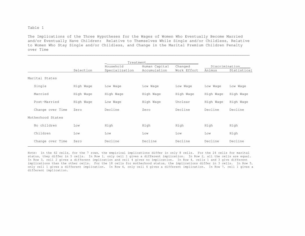
Table 1 The Implications of the Three Hypotheses for the Wages of Women Who Eventually Become Married and/or Eventually Have Children: Relative to Themselves While Single and/or Childless, Relative to Women Who Stay Single and/or Childless, and Change in the Marital Premium Children Penalty over Time ________________________________________________________________________________________________ _ Treatment_________________________ Household Human Capital Changed Discrimination_____ Selection Specialization Accumulation Work Effort Animus Statistical Marital States Single High Wage Low Wage Low Wage Low Wage Low Wage Low Wage Married High Wage High Wage High Wage High Wage High Wage High Wage Post-Married High Wage Low Wage High Wage Unclear High Wage High Wage Change over Time Zero Decline Zero Decline Decline Decline Motherhood States No children Low High High High High High Children Low Low Low Low Low High Change over Time Zero Decline Decline Decline Decline Decline ___________________________________________________________________________________________________________ Note: In the 42 cells, for the 7 rows, the empirical implications differ in only 8 cells. For the 24 cells for marital status, they differ in 5 cells. In Row 1, only cell 1 gives a different implication. In Row 2, all the cells are equal. In Row 3, cell 2 gives a different implication and cell 4 gives no implication. In Row 4, cells 1 and 3 give different implications than the other cells. For the 18 cells for motherhood status, the implications differ in 3 cells. In Row 5, only cell 1 gives a different implication. In Row 6, only cell 6 gives a different implication. In Row 7, cell 1 gives a different implication.

1980-1984 1985-1989 1990-1994 1995-1997Percent:

Single 15.53 20.07 22.51 26.13Married 79.26 73.52 69.79 65.62Widowed .25 .25 .27 .28Divorced 3.15 4.19 5.21 5.96Separated 1.80 1.97 2.22 2.02

No children 25.35 28.71 29.33 29.83First child 19.06 20.43 22.20 21.19Second child 37.81 35.64 33.60 32.54Third+ child 17.78 15.22 14.86 16.44

Basic education 60.85 58.00 53.22 49.94College 7.46 8.06 9.95 11.18Graduate 2.03 3.28 4.87 5.87Professional 24.34 25.43 27.63 29.48Unknown 5.32 5.23 4.33 3.54

Percent Promoted Among:Single 12.89 9.87 9.48 10.70Married 9.35 7.37 7.06 7.28Widowed 6.05 4.21 5.64 7.95Divorced 7.95 5.99 5.56 6.36Separated 8.18 6.90 5.70 6.75

No children 12.27 9.68 8.56 9.67First child 9.71 7.50 7.39 7.26Second child 9.16 7.16 6.81 7.63Third+ child 8.16 6.88 7.14 7.23

Wage relative to singles/childless:Married 1.20 1.20 1.19 1.20Widowed 1.17 1.19 1.16 1.17Divorced 1.18 1.16 1.14 1.13Separated 1.18 1.19 1.15 1.15

First child 1.08 1.09 1.08 1.07Second child 1.16 1.16 1.14 1.15Third+ child 1.17 1.17 1.17 1.19

Experiencemean 16.44 16.71 17.43 17.52sd 7.83 7.94 7.80 7.73

N person-years 241277 257754 271703 155867N individuals 80371 88795 86384 66941N occupations 22 22 22 22N establishments 3810 4057 4293 3468N occ-est 23076 23746 33292 17738

Note: For each year in the data we computed the distributions (in percent) on marital status, parenthood status, educational attainment, and also means and standard deviations for experience. For employees who were present in data in at least two adjacent years, we computed the percent promoted between two years for each marital status and for each parenthood status. We also computed the average wage for each marital and parenthood status as proportion of average wage of single and childless employees. The statistics above have been computed separately for each year, but have then been averaged across years within each of four time periods. The five last lines of the table we give (1) the number of individual-years in each of the four time periods, (2) the number of distinct individuals in each of the four periods, (3) the number of occupations each year, (4) the average number of establishments each year within each of the four time periods, (5) the average number of occupation-establishments units each year within each of the four time periods. Note that on average, employees are observed for a period of 9 years in the data.

Table 2 Descriptive Statistics: Computed Separately by Years, But Averaged Across Years within Each of Four Periods (1980-1984, etc.)

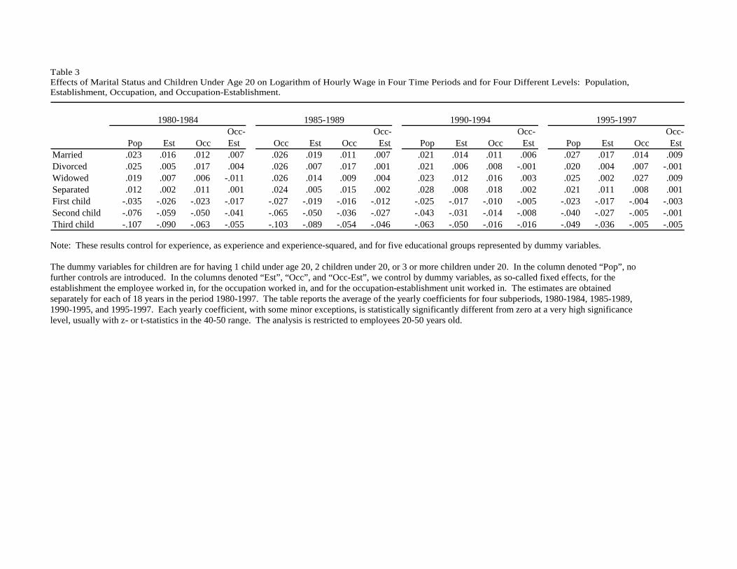
1980-1984 1985-1989 1990-1994 1995-1997 Occ- Occ- Occ- Occ-

Pop Est Occ Est Occ Est Occ Est Pop Est Occ Est Pop Est Occ EstMarried .023 .016 .012 .007 .026 .019 .011 .007 .021 .014 .011 .006 .027 .017 .014 .009Divorced .025 .005 .017 .004 .026 .007 .017 .001 .021 .006 .008 -.001 .020 .004 .007 -.001Widowed .019 .007 .006 -.011 .026 .014 .009 .004 .023 .012 .016 .003 .025 .002 .027 .009Separated .012 .002 .011 .001 .024 .005 .015 .002 .028 .008 .018 .002 .021 .011 .008 .001First child -.035 -.026 -.023 -.017 -.027 -.019 -.016 -.012 -.025 -.017 -.010 -.005 -.023 -.017 -.004 -.003Second child -.076 -.059 -.050 -.041 -.065 -.050 -.036 -.027 -.043 -.031 -.014 -.008 -.040 -.027 -.005 -.001Third child -.107 -.090 -.063 -.055 -.103 -.089 -.054 -.046 -.063 -.050 -.016 -.016 -.049 -.036 -.005 -.005

Note: These results control for experience, as experience and experience-squared, and for five educational groups represented by dummy variables. The dummy variables for children are for having 1 child under age 20, 2 children under 20, or 3 or more children under 20. In the column denoted “Pop”, no further controls are introduced. In the columns denoted “Est”, “Occ”, and “Occ-Est”, we control by dummy variables, as so-called fixed effects, for the establishment the employee worked in, for the occupation worked in, and for the occupation-establishment unit worked in. The estimates are obtained separately for each of 18 years in the period 1980-1997. The table reports the average of the yearly coefficients for four subperiods, 1980-1984, 1985-1989, 1990-1995, and 1995-1997. Each yearly coefficient, with some minor exceptions, is statistically significantly different from zero at a very high significance level, usually with z- or t-statistics in the 40-50 range. The analysis is restricted to employees 20-50 years old.

Table 3 Effects of Marital Status and Children Under Age 20 on Logarithm of Hourly Wage in Four Time Periods and for Four Different Levels: Population, Establishment, Occupation, and Occupation-Establishment.

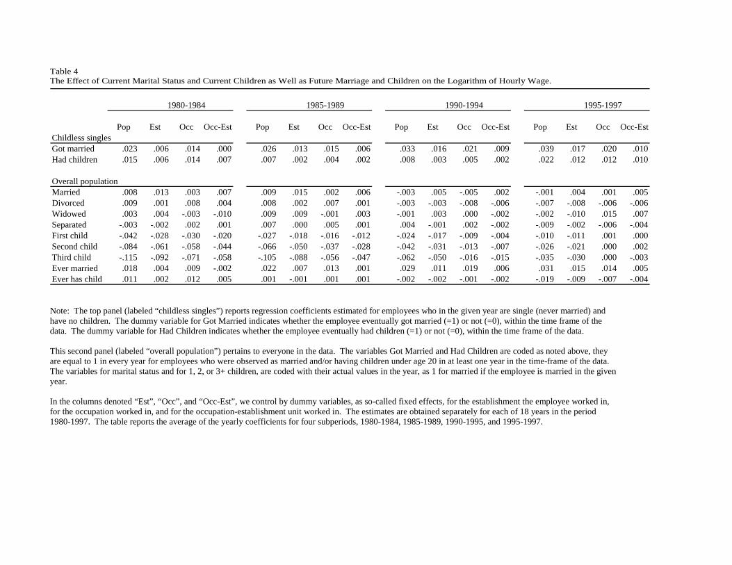
1980-1984 1985-1989 1990-1994 1995-1997

Pop Est Occ Occ-Est Pop Est Occ Occ-Est Pop Est Occ Occ-Est Pop Est Occ Occ-EstChildless singlesGot married .023 .006 .014 .000 .026 .013 .015 .006 .033 .016 .021 .009 .039 .017 .020 .010Had children .015 .006 .014 .007 .007 .002 .004 .002 .008 .003 .005 .002 .022 .012 .012 .010

Overall populationMarried .008 .013 .003 .007 .009 .015 .002 .006 -.003 .005 -.005 .002 -.001 .004 .001 .005Divorced .009 .001 .008 .004 .008 .002 .007 .001 -.003 -.003 -.008 -.006 -.007 -.008 -.006 -.006Widowed .003 .004 -.003 -.010 .009 .009 -.001 .003 -.001 .003 .000 -.002 -.002 -.010 .015 .007Separated -.003 -.002 .002 .001 .007 .000 .005 .001 .004 -.001 .002 -.002 -.009 -.002 -.006 -.004First child -.042 -.028 -.030 -.020 -.027 -.018 -.016 -.012 -.024 -.017 -.009 -.004 -.010 -.011 .001 .000Second child -.084 -.061 -.058 -.044 -.066 -.050 -.037 -.028 -.042 -.031 -.013 -.007 -.026 -.021 .000 .002Third child -.115 -.092 -.071 -.058 -.105 -.088 -.056 -.047 -.062 -.050 -.016 -.015 -.035 -.030 .000 -.003Ever married .018 .004 .009 -.002 .022 .007 .013 .001 .029 .011 .019 .006 .031 .015 .014 .005Ever has child .011 .002 .012 .005 .001 -.001 .001 .001 -.002 -.002 -.001 -.002 -.019 -.009 -.007 -.004

Table 4 The Effect of Current Marital Status and Current Children as Well as Future Marriage and Children on the Logarithm of Hourly Wage.

Note: The top panel (labeled “childless singles”) reports regression coefficients estimated for employees who in the given year are single (never married) and have no children. The dummy variable for Got Married indicates whether the employee eventually got married (=1) or not (=0), within the time frame of the data. The dummy variable for Had Children indicates whether the employee eventually had children (=1) or not (=0), within the time frame of the data. This second panel (labeled “overall population”) pertains to everyone in the data. The variables Got Married and Had Children are coded as noted above, they are equal to 1 in every year for employees who were observed as married and/or having children under age 20 in at least one year in the time-frame of the data. The variables for marital status and for 1, 2, or 3+ children, are coded with their actual values in the year, as 1 for married if the employee is married in the given year. In the columns denoted “Est”, “Occ”, and “Occ-Est”, we control by dummy variables, as so-called fixed effects, for the establishment the employee worked in, for the occupation worked in, and for the occupation-establishment unit worked in. The estimates are obtained separately for each of 18 years in the period 1980-1997. The table reports the average of the yearly coefficients for four subperiods, 1980-1984, 1985-1989, 1990-1995, and 1995-1997.

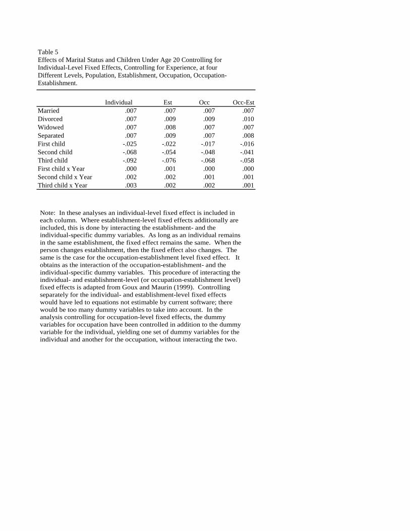
Individual Est Occ Occ-EstMarried .007 .007 .007 .007Divorced .007 .009 .009 .010Widowed .007 .008 .007 .007Separated .007 .009 .007 .008First child -.025 -.022 -.017 -.016Second child -.068 -.054 -.048 -.041Third child -.092 -.076 -.068 -.058First child x Year .000 .001 .000 .000Second child x Year .002 .002 .001 .001Third child x Year .003 .002 .002 .001

Table 5 Effects of Marital Status and Children Under Age 20 Controlling for Individual-Level Fixed Effects, Controlling for Experience, at four Different Levels, Population, Establishment, Occupation, Occupation-Establishment.

Note: In these analyses an individual-level fixed effect is included in each column. Where establishment-level fixed effects additionally are included, this is done by interacting the establishment- and the individual-specific dummy variables. As long as an individual remains in the same establishment, the fixed effect remains the same. When theperson changes establishment, then the fixed effect also changes. The same is the case for the occupation-establishment level fixed effect. It obtains as the interaction of the occupation-establishment- and the individual-specific dummy variables. This procedure of interacting the individual- and establishment-level (or occupation-establishment level) fixed effects is adapted from Goux and Maurin (1999). Controlling separately for the individual- and establishment-level fixed effects would have led to equations not estimable by current software; there would be too many dummy variables to take into account. In the analysis controlling for occupation-level fixed effects, the dummy variables for occupation have been controlled in addition to the dummyvariable for the individual, yielding one set of dummy variables for the individual and another for the occupation, without interacting the two.

1980-1984 1985-1989 1990-1994 1995-1997

Pop Est Occ Occ-Est Pop Est Occ Occ-Est Pop Est Occ Occ-Est Pop Est Occ Occ-EstWage ChangeMarried -.0021 -.0022 -.0021 -.0027 -.0011 -.0008 -.0008 -.0008 -.0001 -.0008 -.0001 -.0009 -.0013 -.0017 -.0017 -.0017Divorced -.0010 -.0012 -.0008 -.0012 -.0006 -.0005 -.0005 -.0005 -.0004 -.0007 -.0002 -.0013 .0000 -.0013 .0001 -.0006Widowed -.0017 -.0019 -.0016 -.0036 -.0004 .0018 .0000 .0014 .0027 .0012 .0015 -.0019 -.0025 -.0019 -.0031 -.0059Separated .0005 -.0013 .0009 -.0015 .0000 -.0008 -.0004 -.0012 .0003 -.0001 .0000 -.0018 .0010 .0006 -.0005 -.0013First child .0003 .0014 .0002 .0016 .0012 .0010 .0011 .0014 -.0002 -.0006 -.0001 -.0001 -.0022 -.0016 -.0021 -.0009Second child .0094 .0102 .0094 .0102 .0080 .0073 .0075 .0073 .0034 .0031 .0031 .0029 .0025 .0030 .0025 .0026Third child .0078 .0101 .0083 .0101 .0112 .0099 .0095 .0090 .0041 .0035 .0037 .0042 .0015 .0024 .0011 .0016

PromotionsMarried .0046 .0045 .0084 .0060 .0115 .0089 .0161 .0115 .0043 .0026 .0059 .0023 .0038 .0012 .0053 .0031Divorced .0054 .0042 .0063 .0017 .0141 .0092 .0157 .0071 -.0008 -.0022 .0027 -.0044 .0072 .0070 .0105 .0074Widowed .0155 .0078 .0194 .0088 .0084 .0017 .0122 .0072 -.0037 -.0089 .0017 .0003 -.0110 -.0149 -.0085 -.0208Separated .0134 .0091 .0164 .0047 .0120 .0054 .0164 .0039 .0030 .0000 .0056 -.0035 .0049 .0056 .0085 .0039First child .0075 .0038 .0027 .0011 -.0022 -.0034 -.0058 -.0082 -.0036 -.0050 -.0081 -.0079 -.0051 -.0044 -.0093 -.0084Second child .0117 .0103 .0022 -.0010 .0075 .0074 -.0036 -.0036 .0000 -.0020 -.0076 -.0055 .0014 -.0003 -.0069 -.0099Third child .0152 .0106 -.0006 -.0226 .0014 -.0013 -.0173 -.0234 .0052 -.0031 -.0081 -.0131 -.0063 -.0043 -.0154 -.0142

Note: The regressions also control for experience, as experience and experience-squared, and for five educational groups represented by dummy variables. The dummy variables for children are for having 1 child under age 20, 2 children under 20, or 3 or more children under 20. In the column denoted “Pop”, no further controls are introduced. In the columns denoted “Est”, “Occ”, and “Occ-Est”, we control by dummy variables, as so-called fixed effects, for the establishment the employee worked in, for the occupation worked in, and for the occupation-establishment unit worked in. The estimates are obtained separately for each of 18 years in the period 1980-1997. The table reports the average of the yearly coefficients for four subperiods, 1980-1984, 1985-1989, 1990-1995, and 1995-1997. The wage change and promotion analyses were restricted to employees who stayed in the same establishment between two adjacent years. The promotion analyses additionally restricted to those who were in the same career ladder between two adjacent years.

Table 6 Effects of Marital Status and Children Under Age 20 on Change in Logarithm of Hourly Wage and Promotion in Occupational Rank Between Two Adjacent Years in Four Time Periods and for Four Different Levels: Population, Establishment, Occupation, and Occupation-Establishment Controlling for Education and Experience.