IRLE

IRLE WORKING PAPER#100-03

November 2003

Marko Tervio

Mediocrity in Talent Markets

Cite as: Marko Tervio. (2003). “Mediocrity in Talent Markets.” IRLE Working Paper No. 100-03. http://irle.berkeley.edu/workingpapers/100-03.pdf

irle.berkeley.edu/workingpapers

eScholarship provides open access, scholarly publishingservices to the University of California and delivers a dynamicresearch platform to scholars worldwide.

Institute for Research on Labor andEmploymentUC Berkeley

Title:Mediocrity in Talent Markets

Author:Tervio, Marko, University of California, Berkeley

Publication Date:11-06-2003

Series:Working Paper Series

Publication Info:Working Paper Series, Institute for Research on Labor and Employment, UC Berkeley

Permalink:http://escholarship.org/uc/item/7411j2vx

Keywords:workforce productivity

Abstract:A model of a labor market is proposed where the level of individual talent can only be learnedon the job and where job positions are scarce. Inability to commit to long-term contracts leavesfirms with insufficient incentives to hire novices, causing them to bid excessively for the pool ofrevealed talent instead. This causes the market to be plagued with too many mediocre workersand inefficiently low output levels, while simultaneously raising the wages for high talents. Thisproblem is most severe where information about talent is initially very imprecise but revealedrelatively quickly on the job. I argue that high incomes in professions such as entertainment,team sports, and entrepreneurship, may at least partly be explained by the nature of the talentrevelation process in those markets. I suggest historical episodes that could be used to identifythe inefficiency and the excessive talent rents predicted by the model.

Copyright Information:All rights reserved unless otherwise indicated. Contact the author or original publisher for anynecessary permissions. eScholarship is not the copyright owner for deposited works. Learn moreat http://www.escholarship.org/help_copyright.html#reuse

Mediocrity in Talent Markets

Marko Terviö∗

Haas School of BusinessUniversity of California, Berkeley

marko@haas.berkeley.edu

November 6, 2003

Abstract

A model of a labor market is proposed where the level of individualtalent can only be learned on the job and where job positions are scarce.Inability to commit to long-term contracts leaves firms with insufficientincentives to hire novices, causing them to bid excessively for the poolof revealed talent instead. This causes the market to be plagued withtoo many mediocre workers and inefficiently low output levels, whilesimultaneously raising the wages for high talents. This problem is mostsevere where information about talent is initially very imprecise butrevealed relatively quickly on the job. I argue that high incomes inprofessions such as entertainment, team sports, and entrepreneurship,may at least partly be explained by the nature of the talent revelationprocess in those markets. I suggest historical episodes that could be usedto identify the inefficiency and the excessive talent rents predicted by themodel.

JEL codes J31, D30.

∗This paper is based on Chapter 1 of my Ph.D. Thesis. I am grateful to Abhijit Banerjee,Emek Basker, Shawn Cole, Frank Fisher, Robert Gibbons, Ben Hermalin, Lakshmi Iyer,Timothy Mueller, Simon Johnson, Eric Van den Steen, Scott Stern, Florian Zettelmeyer,and especially Bengt Holmström and David Autor for comments and suggestions. I thankthe Yrjö Jahnsson Foundation for financial support.

1 Introduction

This paper presents a model of a talent market where industry-specific talent can only be

revealed on the job and publicly. The two crucial features of the model are that individuals

have finite lives and that output has finite demand. This results in a scarcity of both

revealed talent and of job slots. The market price of output has an important role in

determining wages: it must adjust to accommodate the hiring of novices, without which the

industry would run out of workers. I show that, when output and information about worker

productivity are jointly produced, then typical labor market imperfections yield an artificial

scarcity of known talent, too little exit from the industry, and artificially high talent rents.

When individuals cannot commit to long-term wage contracts, the value of information

accrues as rents to those who turn out to be high talents and see their wages bid up, while the

firms that hired them do not get rewarded for the discovery. Unless individuals are able to

pay for the opportunity to reveal their talent, firms will only take into account their expected

talent for the near term and ignore the upside potential of previously untried individuals.

Firms then prefer to hire someone who is known to be even slightly above the population

mean to hiring a novice of unknown type. There is thus an inefficiently low level of exit from

the industry, especially by relatively inexperienced workers. If talent is revealed relatively

quickly, then most of the active workforce may consist of “mediocre” types who would exit

the industry in the efficient solution. Instead they stay in the industry, producing output

that crowds out entry by novices. The industry as a whole has what is in effect an up-or-out

rule, but this rule is unduly lenient.1

If individuals were risk neutral and had sufficient funds, then previously untried individ-

uals would be able to pay for the chance to find out their talent level, up to the expected

value of their lifetime talent rents. This would lead to an efficient solution, where even

relatively high talents exit the industry if their job slots have higher social value in trying

to discover even higher talent. With uncertain return to such talent (i.e. when talent rents

mostly accrue to a minority of very successful individuals) the willingness of young individ-

1Efficient up-or-out rules are possible when information is match-specific; see e.g., O’Flaherty and Siow

(1995). For a signalling perspective to up-or-out rules see Waldman (1990) or Kahn and Huberman (1988).

1

uals to pay for future rents can be much below the expected value. Credit constraints or

even moderate levels of risk aversion can cause the market outcome to deviate considerably

from full efficiency.

Perhaps surprisingly, the opportunity to save aggravates the inefficiency caused by a

credit constraint. Saving by “has-been” individuals who perform well early in their career,

but who fall below population mean in expected talent later, allows them to outbid credit

constrained novices. Their incentive to pay for job slots is the chance of more talent rents

in the future: since talent is only revealed over time, the has-beens still retain some upside

potential, albeit less than the novices. However, after sufficiently bad performance even the

has-beens exit, regardless of their savings.

This paper provides a plausible explanation for high and skewed wages in many industries

that appear to have high talent rents. As an explanation, it is complementary to theories

based on scale effects2 (see, e.g.,Lucas 1978 and Rosen 1982) and superstar economics (Rosen

1981), even though less benign in the sense that it is associated with possibly dramatic ineffi-

ciencies. These papers are concerned with the efficient allocation of capital (and consumers)

to known talent, whereas the focus here is on the discovery process of talent. For example,

we might wonder why some alternative manager wouldn’t be nearly as good as the current

CEO with his exorbitant compensation, scale effects notwithstanding. This paper shows how

the supply of talent, as observed in the market, can be very scarce even when it is not so

in the population; and, more importantly, revealed talent can be much more scarce than it

need be due to the twin imperfection of spot contracts and credit-constrained (or risk averse)

individuals.

This paper also provides predictions about what kind of talents and industries could be

expected to exhibit high and uneven wages. Inasmuch as a talent market fits the assumptions

of the model, it can be expected to be flooded by too many mediocre workers. Such a market

would react to certain exogenous changes, particularly to individual commitment ability and

to access to credit, in ways that could be used to identify and quantify the inefficiencies

described in the model. The benefit from ameliorating market imperfections comes through

2With a scale effect or “scale-of-operations effect” differences in talent are accentuated when higher talent

is matched with more productive complementary resources, such as capital.

2

higher exit rates for young workers, a prediction at odds with standard training and human

capital models. Higher exit rates would in turn show up as increased productivity, lower

wages and decreased wage dispersion.

In this paper talent corresponds to level of output. Jobs within an industry are homoge-

neous, as if all workers operated identical “machines.” To say that one individual is twice as

talented as another means that he produces twice as much output (possibly in expectation,

or in quality-adjusted “hedonic” units). The economic value of talent is endogenous and de-

pends on the equilibrium price of output. Under this definition of talent, it is meaningful to

consider a thought experiment where the distribution of talent is the same in two industries.

In order to focus on learning, several commonly studied features of labor markets are

assumed away in this paper. There is no on-the-job training or learning-by-doing, so ex-

perience per se is not economically valuable. Neither are there any frictions such as hiring

or firing costs, nor any organizational capital to speak of. Information is symmetric at all

times: there are no effort problems, career concerns, or adverse selection. The homogeneity

of job slots rules out any problems with job assignment within the industry.

The inefficiency described here could, in principle, be identified given a suitable natural

experiment. An exogenous change in individuals’ commitment ability would be ideal. For

example, the end of the studio system in the motion picture industry in the 1940s is a change

that the model predicts would lead to rehiring of mediocre talent. Under the studio system,

young actors were able to commit to long-term contracts with motion picture companies.

Available stylized facts of decreased revenue and output, as well as the casual evidence of

increased wages, are consistent with the predictions of the model. However, contemporaneous

changes, in particular the advent of television, make it difficult to draw strong conclusions.

The joint production problem of output and information about worker quality has been

well understood since Johnson (1978) and Jovanovic (1979). The social planner’s solution in

this type of problems draws on the “bandit” literature (see, e.g.,the treatise by Gittins, 1989,

and Miller, 1984, who uses the bandit approach in a multi-sector setting). MacDonald (1988)

presents a stochastic version of Rosen’s superstars model, where superstars are selected

based on earlier performance. These papers solve for the efficient equilibrium; the focus here

is on how the market handles the discovery of talent under the constraints to individual

3

credit and commitment ability. In this way, the model is analogous to setups where firms

should give training in general skills but don’t have sufficient incentives, due to the same

standard labor market imperfections. This literature uses additional imperfections, typically

asymmetric information (proposed by Greenwald 1986), to give firms incentives to train (see,

e.g.,Acemoglu and Pischke, 1998).

The plan of the paper is as follows. In Section 2, a numerical example is used to illustrate

the basic ingredients of the model. Section 3 presents the basic model of a talent market,

with the simplest possible revelation process: individual talent is initially unknown, and then

becomes public knowledge after one period on the job. Mediocrity and the loss associated

with inefficient hiring are defined in an empirically quantifiable way. Section 4 extends the

model to many periods, with talent revealed gradually over time. This makes it possible

to study the effects of saving. Section 5 discusses the relevance of the findings for real-

world talent markets, and suggests possible natural experiments to identify and quantify the

welfare cost of mediocrity. Section 6 concludes the paper.

2 Example: A Simple Talent Market

Consider a competitive industry that combines workers with capital (machines for producing

output). There is free entry by firms, which each need one worker to operate one machine

that has a rental cost of $4 million.3 All units of output are identical, and the amount of

output that a firm produces depends solely on the talent of its worker (later in the paper it

will be more natural to interpret talent as affecting quality, and the market price as being

for hedonic “quality-adjusted” units of output). There is an unlimited supply of potential

workers with an outside wage of zero (outside meaning outside the industry). A novice is

equally likely to produce anywhere between zero and one hundred units.4 The talent of a

novice worker is unknown (including to himself), but becomes public knowledge after one

period of work. Careers are finite and last at most 16 periods. Workers cannot commit to

decline higher outside wage offers in the future. Industry output faces a downward-sloping

3All numbers in this example are chosen for convenience.4For example, the machine could have a capacity for one hundred units per period, and talent could

determine the proportion of successfully completed units.

4

demand curve, and the number of firms is “large,” so that firms take the market price as

given and there is no aggregate uncertainty. Finally, for simplicity, there is no discounting.

How does this talent market work? That depends crucially on whether aspiring workers

can pay for the opportunity to work. There are two extreme cases to consider. In the first,

individuals are constrained to take a non-negative wage. This is the inefficient, but at the

same time also the more straightforward case. In the second case, individuals are risk neutral

and not credit-constrained. Due to the absence of imperfections, this is, not surprisingly,

the efficient benchmark.

The purpose of the example is to compare the distribution of talent and wages in the

industry under these two cases. Only the steady state is considered, where the number of

entering and exiting workers is constant over time.

Constrained Individuals

In this case, all workers who turn out to be above the population mean (i.e., those who were

able to make 50 units or more) will stay in the industry until they retire. These veterans

create more revenue than a novice in expectation, so they can always outcompete them for

a job in this industry.

The market price of output must be such that novice-hiring firms break even. Since

potential novices are not scarce, they will always be paid zero. A novice is expected to make

50 units, so an output price of ($4 million)/(50 units)= $80, 000 ($80K) per unit is needed

to cover the capital cost. At this price there is no entry or exit of firms from the industry.

Veteran workers are always scarce. Due to free entry, firms cannot make positive profits

and will bid up the wages of veteran workers, who get the difference between their revenue-

generating capacity and that of a novice as a Ricardian rent. In particular, the highest type

produces 50 more units than a novice or an average type. Therefore at the price of $80K

per unit, top veterans get 50× $80K = $4 million per period. The average wage of veterans

is $2 million (since talent is uniformly distributed).

Because production cost per worker is fixed, the efficiency at which the demand for

output is satisfied depends solely on the average talent of workers in the industry. The

average output by veterans is 75 units; the average for the whole industry must be lower

5

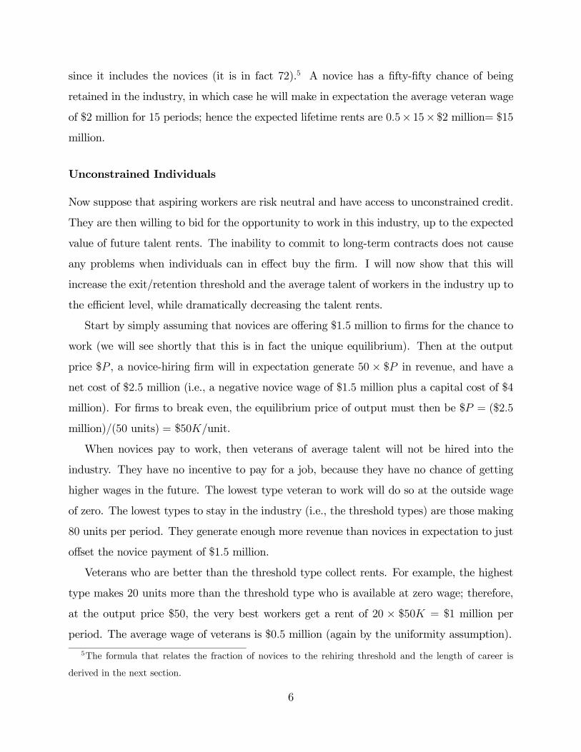
since it includes the novices (it is in fact 72).5 A novice has a fifty-fifty chance of being

retained in the industry, in which case he will make in expectation the average veteran wage

of $2 million for 15 periods; hence the expected lifetime rents are 0.5× 15× $2 million= $15

million.

Unconstrained Individuals

Now suppose that aspiring workers are risk neutral and have access to unconstrained credit.

They are then willing to bid for the opportunity to work in this industry, up to the expected

value of future talent rents. The inability to commit to long-term contracts does not cause

any problems when individuals can in effect buy the firm. I will now show that this will

increase the exit/retention threshold and the average talent of workers in the industry up to

the efficient level, while dramatically decreasing the talent rents.

Start by simply assuming that novices are offering $1.5 million to firms for the chance to

work (we will see shortly that this is in fact the unique equilibrium). Then at the output

price $P , a novice-hiring firm will in expectation generate 50 × $P in revenue, and have a

net cost of $2.5 million (i.e., a negative novice wage of $1.5 million plus a capital cost of $4

million). For firms to break even, the equilibrium price of output must then be $P = ($2.5

million)/(50 units) = $50K/unit.

When novices pay to work, then veterans of average talent will not be hired into the

industry. They have no incentive to pay for a job, because they have no chance of getting

higher wages in the future. The lowest type veteran to work will do so at the outside wage

of zero. The lowest types to stay in the industry (i.e., the threshold types) are those making

80 units per period. They generate enough more revenue than novices in expectation to just

offset the novice payment of $1.5 million.

Veterans who are better than the threshold type collect rents. For example, the highest

type makes 20 units more than the threshold type who is available at zero wage; therefore,

at the output price $50, the very best workers get a rent of 20 × $50K = $1 million per

period. The average wage of veterans is $0.5 million (again by the uniformity assumption).

5The formula that relates the fraction of novices to the rehiring threshold and the length of career is

derived in the next section.

6

Finally, to show that this is the equilibrium, calculate the expected lifetime rents. A

novice has a 20% chance of turning out to be above the 80 unit threshold, in which case his

expected wage is the average veteran wage of $0.5 million for the last 15 periods. Expected

lifetime rents are then 0.2× 15× $0.5 million= $1.5 million, which was the assumption we

started from. This is also the unique equilibrium, because higher offers by novices increase

the exit threshold and thus decrease the expected rents.

The average output of veteran workers is 90 units (because veteran talent is uniform

between 80 and 100). The industry average is lower, because some workers are novices; in

fact it must be exactly 80 units per worker. That the optimal (i.e., maximal) average talent

level of workers is the same as the optimal exit threshold is a general result (in this limiting

case of a zero discount rate). Intuitively, if at the optimum some level of talent gets discarded

from the industry then it must be pulling down the industry average, while a talent that is

retained must be increasing it.

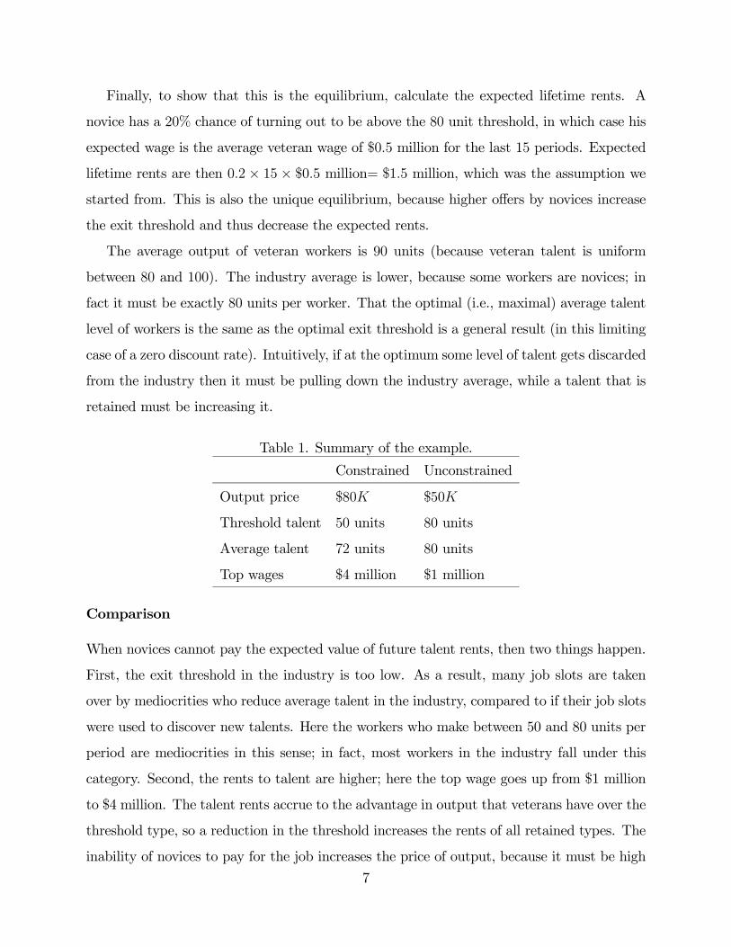
Table 1. Summary of the example.

Constrained Unconstrained

Output price $80K $50K

Threshold talent 50 units 80 units

Average talent 72 units 80 units

Top wages $4 million $1 million

Comparison

When novices cannot pay the expected value of future talent rents, then two things happen.

First, the exit threshold in the industry is too low. As a result, many job slots are taken

over by mediocrities who reduce average talent in the industry, compared to if their job slots

were used to discover new talents. Here the workers who make between 50 and 80 units per

period are mediocrities in this sense; in fact, most workers in the industry fall under this

category. Second, the rents to talent are higher; here the top wage goes up from $1 million

to $4 million. The talent rents accrue to the advantage in output that veterans have over the

threshold type, so a reduction in the threshold increases the rents of all retained types. The

inability of novices to pay for the job increases the price of output, because it must be high

7

enough to cover the cost of production at novice-hiring firms. This increased price further

magnifies the rents to retained talent.

3 The Basic Model

This section introduces the basic model of a competitive talent market. Here I will solve for

the equilibrium distribution of talent, wages, and tenure, with and without the presence of

standard labor market imperfections.

Model assumptions

1. Each firm employs one individual per period, has production cost c, and output equal

to the talent of the worker, θ.

2. There is an unlimited supply of individuals with unknown talent, willing to work at

outside wage w0.

3. A worker’s talent level becomes public after one period in the industry. He can then

work in the industry up to T more periods (1 + T periods in total).

4. Talent is drawn from a distribution with a continuous and strictly increasing cumulative

distribution function, F (•), with support [θmin, θmax].

5. There is no discounting. Firms are infinitely lived and maximize average per-period

profits.

6. There is free entry by firms.

7. The number of firms I is treated as a continuous variable (measure).

8. Industry output faces a downward-sloping demand function Qd(P ).

The first assumption describes the technology. The firms are identical; all differences in

output are caused by the talent of the worker.

Assumptions 2 and 3 describe the information structure. That all uncertainty about

talent is resolved after one period of work is a simplification of the idea that information about

8

the talent of a novice is much less precise than that of experienced individuals. Information

is symmetric at all points in time: firms (as well as individuals themselves) view all novices

as identical, so they are expected to have the mean talent level θ. After one period of work,

an individual’s output (i.e. his talent) becomes public.

Assumptions 4 and 5 are not essential but are made for technical and notational conve-

nience. Assumptions 6 and 7 result in a competitive industry that is “large” in the sense

that there is no uncertainty about the realization of the distribution of talent. Assumption

8 closes the model.

The assumed labor market imperfections are standard:

A. Individuals cannot commit to long-term contracts.

B. Individuals cannot take a wage below some w0 ≥ 0.

The case with both two assumptions is the more realistic case in most industries and will be

referred to as the case of “constrained individuals.” In terms of missing markets, assumption

A means that individuals cannot sell their future labor. Assumption B approximates the idea

that the ability of novices to pay for future talent rents is small compared to their expected

value. This could result from a credit constraint, or from individual risk aversion coupled

with the inability to insure against realizations of one’s own talent level. Removal of either

assumption would allow the industry to operate efficiently. The case with assumption A, but

without B, will be referred to as the case of “unconstrained individuals,” because it allows

individuals in effect to “buy the firm” and thus bypasses the problem of commitment. On

the other hand, in the absence of Assumption A novices would sign up to lifelong contracts

at the outside wage w0 (with firms retaining the right to fire the worker).

Preliminaries

The equilibrating variable is the exit threshold ψ; it will be shown later that the measure of

jobs I will be determined mechanically given the threshold. Those who turn out to have a

talent level below the threshold leave the industry after just one period. Vacancies left by

novices who were not good enough to make the grade and by those retiring must be filled

by new novices. In this preliminary section I derive the relation of the exit threshold, the

equilibrium fraction of novices, and the average level of talent in the industry. With a given

9

exit threshold, this is just a matter of equating the flows of entry and exit.

Denote the fraction of novices by i. When dealing with the distribution of talent, we

can without loss of generality think of the industry as consisting of a unit mass of jobs.

Consider only the steady state, where i is constant over time. Each period, the talents of i

new workers are revealed, and of these a fraction F (ψ) exit. The remaining 1− i jobs in the

industry must be held by veterans; of these the oldest cohort, a fraction 1Tof all veterans,

retires each period. Equating exit and entry yields

iF (ψ) +1

T(1− i) = i =⇒

i(ψ) =1

1 + T (1− F (ψ)).(1)

The exit threshold further determines the average talent of workers in the industry. Denote

the average talent in the industry by

(2) A ≡ iθ + (1− i)E[θ|θ > ψ].

Clearly A will be above the population mean θ, because types above the threshold will work

for longer than the below-threshold types. Only if there were no filtering at all would the

industry average be equal to the population mean. Substituting the equilibrium fraction of

novices (1) into (2) yields the industry average as a function of the exit threshold.

(3) A(ψ) =1

1 + T (1− F (ψ))θ +

T (1− F (ψ))

1 + T (1− F (ψ))E[θ|θ > ψ]

Note that total industry output is the measure of firms times the average level of talent in

the industry.

Social Planner’s Problem

Consider the problem of maximizing social surplus

(4) S(I, ψ) =

Z IA(ψ)

0

P (q)dq − I (w0 + c) ,

where P (q) is the inverse of the demand function Qd(P ) and I the level of employment

(measure of firms). Social surplus is the consumer surplus from total output, minus the

opportunity cost of the factors of production. The problem of choosing the efficient exit

10

threshold is independent of the size of the industry: for any I, the threshold ψ should

be chosen to maximize the average level of talent A in the industry. This will minimize

average costs, because cost per job is constant w0 + c. The level of employment should

then be chosen to equate total output with demand at the minimized average cost, so that

P (IA) = (w0 + c)/A. The industry as a whole has constant returns to scale: to double

the output, the amount of novices hired and total costs would both be doubled; this would

(eventually) double the number of veterans as well.

To maximize the average talent (3), take the first-order condition:

∂

∂ψA(ψ) =

∂

∂ψ

µ1

1 + T (1− F (ψ))

½θ + T

Z θmax

ψ

af(a)da¾¶

= 0

=⇒ T f(ψ)

(1 + T (1− F (ψ)))2©θ + T (1− F (ψ))E[θ|θ > ψ]

ª− T ψf(ψ)

1 + T (1− F (ψ))= 0

=⇒ θ + T (1− F (ψ))E[θ|θ > ψ] = ψ (1 + T (1− F (ψ))) .(5)

The first order condition (5) can be rearranged to yield the following condition:

(6) ψ − θ = T (1− F (ψ)) (E[θ|θ > ψ]− ψ) .

Denote the solution henceforth by A∗.6 To interpret (6), think of the decision to hire a novice

over a veteran of above-average talent as an investment. The LHS gives the immediate loss

in expected output from hiring a novice instead of the threshold veteran. The RHS shows

the expected future gain, assuming that ψ is also kept as the rehiring threshold in the future.

The trade-off is that a higher threshold results in higher-quality veterans, but also in a larger

fraction of the workforce being novices.

It is useful to notice that the maximizer of (3) is also its unique fixed point in the support

of θ.

Proposition 1 maxψ A(ψ) = argmaxψ A(ψ) > θ.

6For example, the uniform [0,1] distribution used in the example of Section 2 yields the solution

(7) A∗ =1

T

³1 + T −

√1 + T

´.

11

Proof. First, to see that the solution to (6) is a fixed point of A, solve the linear term

in ψ and then divide both sides by 1+T (1− F (ψ)). This reproduces the objective function

(3). Second, to see that the solution exists, is unique, and strictly greater than θ, notice that

the LHS of (6) is strictly increasing, and equal to zero at ψ = θ. The RHS is decreasing,

starts from positive T (θ − θmin) at ψ = θmin and reaches zero at ψ = θmax.¤In other words, the optimal exit threshold is also the maximum attainable average level

of talent in the industry: A∗ = A(A∗). Intuitively, discarding a worker above the optimal

threshold must decrease the average, as must retaining a worker below the threshold.7 The

optimal level of employment equates supply IA∗ with demand at average cost (w0 + c) /A∗,

so I∗ ≡ 1A∗Q

d(w0+cA∗ ).

Definition 1. Mediocre types: θ ∈ (θ, A∗). These are the talent levels above the

population mean, but below the optimal rehiring threshold.

In other words, “mediocrities” are people are better than average but who should not be

working in the industry.

Market Equilibrium

Like the social planner’s allocation, market equilibrium can also essentially be described

by the exit threshold ψ. The level of equilibrium threshold will depend on the presence

of market imperfections, but, for a given threshold, we can already deduce the equilibrium

wages, output price, and employment. In any case, the individual inability to commit to

long-term contracts means that wages are determined on a spot market. Equilibrium wages

must therefore keep firms indifferent between hiring any worker in the industry for the

next period. This means that (expected) differences in talent translate into corresponding

differences in wages, and into Ricardian rents for inframarginal talents. At the same time,

the price of output must adjust to allow the hiring of novices into the industry, while free

entry keeps profits at zero.

Proposition 2 w(ψ) = w0.

7With discounting the maximizer would be below the maximum. Reducing the rehiring threshold amounts

to a reduction in investment (the amount of experimentation with new talent), which leads eventually to a

lower average level of talent in the industry.

12

Proof. Since veterans have no future payoffs to think about, their decision to stay

depends solely on whether the wage they can get inside the industry is more than the

outside wage. With a continuum of types, the lowest type veteran to work in the industry

must be indifferent and therefore paid exactly the outside wage.¤

Proposition 3 Given an equilibrium exit threshold ψ, the price of output is P = (w0 + c) /ψ.

Proof. Due to free entry firms must make zero profits. In particular, a firm employing

a veteran of the threshold type ψ gets revenue Pψ and has costs w0 + c. The equilibrium

price sets these equal.¤The combination of free entry by firms and a binding outside wage for veterans of thresh-

old type pins down the price of output.

Proposition 4 Given an equilibrium exit threshold ψ, wages are

(8) w(θ) = (w0 + c)

µθ

ψ− 1¶+ w0.

Proof. For firms to be indifferent between a threshold type ψ and any other talent θ,

the difference in wages must just offset the difference in revenue generated. Hence for any θ

(9) w(θ)− w(ψ) = P (θ − ψ) =

µw0 + c

ψ

¶(θ − ψ) .

Combining this with Proposition 2 completes the proof.¤

Proposition 5 Given an equilibrium threshold ψ, employment is

(10) I(ψ) =1

A(ψ)Qd

µw0 + c

ψ

¶.

Proof With threshold ψ and employment I the supply of output is IA(ψ), that is,

the measure of workers times their average output. Set the supply equal to demand Qd(P ),

substituting in the output price from Proposition 3, and solve for I.¤

13

Constrained Individuals The wage equation from Proposition 4 must also apply to

novice wages: from the firms’ point of view, novices are just workers with talent equal to

population mean θ. In the constrained case, novices must always get paid exactly w0. They

cannot get more, because they are not scarce, and they cannot subsist on less by assumption.

However, workers that have been revealed to be above the population mean are necessarily

scarce; they are earning rents and have no reason to exit. In terms of the wage equation (8) we

have the exit threshold at ψ = θ. And, as we know from Proposition 1, the population mean

is an inefficiently low rehiring threshold: average talent in the industry is not maximized at

A(θ).

If a firm hires a novice that turns out to be above average, his wage will be bid up

by other firms. Therefore firms only care about the expected ability of a worker for the

current period. They fail to take into account the upside potential of young individuals, who

themselves are not able to pay for the chance to make talent rents in the future.

Unconstrained Individuals If individuals are risk neutral and have access to sufficient

funds, then they will bid for the chance to enter the industry up to the expected value of

talent rents. By offering to pay for the chance to work, unconstrained novices provide firms

with the right hiring and firing incentives. Firms will now hire novices instead of mediocre

veterans who have no incentives to offer such payments–whatever wage they could get

in one period, they will get for the rest of their career. As is intuitive, the payments by

unconstrained novices raise the exit threshold to the efficient level. The role of the firm is

reduced to financing the production cost c in return of a certain market rate of return (set

at zero here).

The efficient exit threshold could also be derived by solving for the market equilibrium in

the unconstrained case, which we know must be efficient. In equilibrium, workers and firms

take the output price P and the exit threshold ψ as given. Since veterans of threshold type

are available at the outside wage, novices have to pay P (ψ− θ) for their first period job slot.8

This payment exactly compensates a novice-hiring firm for the one-period revenue loss that it

expects compared to hiring the threshold type. At the same time, the novice payment must

8So the first period wage is w − P (θ∗ − θ), which could be much below zero.

14

be equal to expected lifetime rents: with threshold ψ, a novice has a probability 1 − F (ψ)

of being retained, in which case he gets the excess revenue P (θ−ψ) as a rent on each of the

T remaining periods of his career. This equality is the market equilibrium condition:

(11) P (ψ − θ) = (1− F (ψ))TP (E[θ|θ > ψ]− ψ) .

The market price P cancels out of the equilibrium condition, which is therefore just the

first-order condition (6) in the social planner’s problem and yields the optimal threshold A∗

as a solution. In addition, the distribution of wages is now also determined. Wages are given

by equation (8), with the exit threshold at ψ = A∗.9 Recalling Proposition 3, the price of

output is therefore equal to minimized average cost P ∗ = (w0 + c) /A∗.

Discussion

To summarize, the main effect of the constraint on novices’ ability to pay for jobs is that

the standard of performance required for an individual to be retained in the industry is too

low. Just as a matter of accounting, the inefficiently low exit rates mean that careers are too

long on average and that the proportion of young workers is too low. Older workers are not

as talented as they could be. The inefficient hiring policy increases talent rents in two ways.

First, rents accrue to the difference in units of output that an individual makes compared

to the threshold type; this is higher for any retained type in the constrained case since the

exit threshold is lower. Second, the value of this advantage is proportional to the price of

output, which is higher in the constrained case: when novices cannot pay for the opportunity

to work, it takes a higher output price to allow novice-hiring firms to break even.

The real curse of mediocrity upon society comes not just from the loss in average out-

put per workers, A∗ − A(θ), but from the increase in output price that is needed to make

novice-hiring feasible. This price increase causes some of potential consumer surplus to be

transferred into rents for the workers in the industry, especially to the most talented. Fur-

thermore, since output is produced less efficiently, more workers are needed to satisfy any

9While risk neutral workers are indifferent between any gambles of the same expected value, it is reasonable

to use the solution that is the unique limit of vanishingly small risk aversion. Note that there are no match-

specific rents and therefore no scope for bargaining.

15

given level of demand. In an industry with sufficiently inelastic demand, the hiring of medi-

ocrities is associated with too many people working in the industry.10 In addition to this

transfer there is of course the deadweight loss from the higher price, whose severity also

depends on the elasticity of demand.

Above the comparison of an efficient and an inefficient market was made between markets

where novices can and cannot pay for jobs. Efficiency could also be achieved by eliminating

the other imperfection, the inability to commit to long-term wage contracts. In that case

novices would commit to lifelong contracts at the outside wage and the talent rents w (θ)−w0would accrue to firms. The rent that was part of a veteran’s wages before would now be

the rental cost of talent. Talent at and below the efficient threshold level A∗ would be

available at zero rental cost, so the initial payment P ∗(A∗ − θ) would be the opportunity

cost borne by a novice-hiring firm (free entry would still guarantee that firms make zero

profits in expectation). While the model itself does not require any turnover between firms,

it is consistent with firms renting workers at the equilibrium rental cost or trading them at

the present value of future rents.

In reality, changes to imperfections are unlikely to be of the all-or-nothing type, but

the direction of the effect of more limited changes should be clear. (A few such potential

episodes are discussed in Section 5.) Any payments by novices would displace the worst

of the mediocrities, thus increasing the exit threshold and reducing the talent rents of all

veterans. Similarly, even a limited commitment time would give firms some incentives to

hire novices instead of the lowest types of mediocrities. They could count on keeping any

talent rents generated during the commitment (when the wage is at w0), after which the

rents accrue to the released veterans or “free agents.” Firms would then choose a hiring

policy that maximizes the average talent of committed workers. The longer the duration

of commitment, the closer the solution is to full efficiency and the lower the wages of free

agents of any given talent.

10This effect is not a case of excess talent rents attracting too many hopefuls to the industry, as in the

story of Frank & Cook (1995), but rather a distortion from an inefficient production method which benefits

the owners of a factor of which too much is used.

16

Monopsony. One implication of inefficient hiring is that a monopoly could serve the con-

sumers better than a competitive industry if demand is sufficiently elastic. Suppose that

the industry could merge into one firm that would be a monopsonist on the talent market.

It would then have the incentives to enforce the socially optimal exit threshold. By being

able to maximize the average level of talent in the industry, a monopolist would therefore

also minimize the average cost of production. With sufficiently elastic demand this would

be enough for the monopoly price to be below the competitive price. For example, with

constant elasticity of demand η, we know that a profit-maximizing monopoly marks up its

price by a factor of η/ (η − 1). Since the competitive output price is (w0+ c)/θ, and monop-

olists’ average cost is (w0 + c)/A∗, it follows that the output price would be lower under a

monopolist if η > A∗/¡A∗ − θ

¢.

The Role of Production Costs. Consider two otherwise identical talent markets with

different production costs. Higher cost means higher output price, meaning higher dollar

value for any given difference in talent. In the case of unconstrained novices, higher ex-

pected rents are offset by an increase in the required novice payment, and the costs have no

effect on the hiring threshold. In the constrained case all mediocrities are rehired regardless

of the production cost. However, in the intermediate case, where novices have some ability

to pay, the distribution of talent in the industry does indeed depend of the cost of produc-

tion. Any payment by novices displaces the worst of the mediocrities, namely those whose

output advantage over the population mean is worth less than the novice payment. With a

higher output price the same amount of payment by novices displaces a narrower range of

mediocrities, so hiring gets lets efficient. In an industry with a low cost of production the

novice payment required for full efficiency is relatively low, so the assumed credit constraint

is also less plausible.

The Role of the Speed of Revelation. The parameter T can be interpreted as the

ratio of veteran time to novice time, with the latter normalized at one. A higher number

of “veteran periods” therefore corresponds to quicker revelation of talent. For any given

exit threshold, quicker revelation means that the average level of talent is higher for the

17

mechanical reason that below-threshold talents spend less time in the industry. In the

constrained case this is the only benefit: the exit threshold is always θ; with higher T the

average talent in the industry gets closer to E[θ|θ > θ] as the below-average types get filtered

out faster. The speed of revelation has no effect on the output price as it is fixed by the

need of novice-hiring firms to break even. However, the social return to the investment of

hiring a novice is increasing in the speed of revelation, and so is the efficient threshold. To

see this, totally differentiate the equilibrium condition (6) with respect to ψ and T , and use

the envelope theorem; this yields

(12)∂A∗(T )

∂T=

1− F (A∗)

1 + T (1− F (A∗)){E[θ|θ > A∗]−A∗} > 0.

For ever faster revelation the efficient threshold and the resulting average talent get closer

to the maximum of the talent distribution. With price equal to average cost this higher

productivity goes entirely to the benefit of the consumers.

The main effect of quicker revelation is to increase the social value of experimentation

with new talent. On the other hand, for quicker revelation the required novice payment (for

normalized lifetime length) to achieve efficiency may also get smaller (in the limit, where

the revelation time goes to zero, it must also go to zero), thus making the assumption of a

binding credit constraint less plausible.

4 Gradual Learning and The Phenomenon of Has-beens

This section extends the model by allowing information about talent to be revealed over

time. While the optimal solution is analogous to that of the basic model, the case of credit

constrained individuals is altered by the opportunity to save. I will show that, instead of

mitigating the inefficiency caused by a credit constraint, saving will actually make things

worse. It lowers exit rates even further below optimal because some veterans of below-average

talent will stay in the industry.

In the basic model, individuals have essentially two-period careers, with the relative

length of the second “veteran” period described by T . All uncertainty about an individual’s

talent is resolved at a single point in time, so the only variable of choice is the exit threshold

18

at that point. When new information about talent arrives at several points in time, then the

decision to continue must take into account the option of exiting at a later time. Without

further constraints, this would be a standard optimal stopping problem, introduced into the

theory of labor markets by Jovanovic (1979). In this section I explore the general implications

of a similar problem, but when job slots are scarce, learning is public and industry-specific,

and individuals have finite careers and cannot commit to long-term contracts.

Assumptions

1. Each firm employs one worker per period whose output is yt = θ + εt, where θ is the

worker’s talent and εt an i.i.d. error term.

2. There is an unlimited supply of individuals willing to work at outside wage w0.

3. Individual careers last up to 1 + T periods.

4. The cumulative distribution functions of θ and ε are strictly increasing, continuous,

and yield finite moments.

5. {θt, t} is a sufficient statistic for θt+1, where θt ≡ E[θ|y1, . . . , yt] is the expected level

of talent at tenure t (i.e. after t periods of work).

The expectation θt is taken with respect to the known distributions fθ and fε. For the

novices, no output has yet been observed, so θ0 = θ for all of them. Since predictions are

unbiased by definition, E[θt+s|θt]= θt for any s = 1, . . . , T − t. Period t perceived talent θt

will often be simply referred to as talent. A crucial implication of the assumptions is that the

distribution of prediction errors does not become degenerate in finite time: there is always

some chance that the individual is better than he is expected to be.

Going forward in time, the estimate of any particular worker’s talent becomes more

precise; it gets closer to the true value in expectation and moves about less. However, a

worker’s talent never becomes known for sure. In terms of a whole cohort, the distribution

fθt starts as a degenerate distribution at θ, and then becomes more spread out. Without

filtering, it would become more like the true distribution fθ; with filtering, more of the lower

types, as well as some unlucky higher types, get discarded as time goes by.

Other assumptions

6. Firms are infinitely lived and maximize average expected per-period profits. There is

no discounting.

19

7. There is a unit measure of firms.

8. Price of output is normalized to one.

These assumptions are made in order to simplify the notation. Extending the analysis to

allow for free entry and an endogenous output price is straightforward in light of section 3.

Social Planner’s Problem

The variable of choice is a stopping (exit) policy ψ = {ψ1, . . . , ψT}, which consists of T

separate exit thresholds. Analogously to the single exit threshold of the basic model, this

policy states that an individual with talent θt < ψt will exit the industry. Since everyone

looks identical at t = 0, there is no meaningful choice for ψ0 (besides θ). On the other hand,

after T + 1 periods, the individual will retire anyway, and the updating of θ based on yT+1

is useless. Hence there are in total T points in time where a decision to continue or stop has

to be made. A decision to exit is final, because after the exit no new information will ever

arrive that could change the decision.

The average level of talent in the industry depends on the whole stopping policy. In line

with earlier notation, denote the maximal solution by A∗ ≡ maxψ A(ψ). This would be the

object of a surplus-maximizing social planner, as well as of a firm who could keep individuals

at a fixed wage. The optimal solution must adhere to the following variant of the fixed point

result in Proposition 1.

Proposition 6 In the optimal solution, ψT = A∗.

The proof is omitted as it is basically the same as in the basic model. Intuitively, given

an individual with just one period left, the optimal decision of whether to retain him or not

depends solely on his expected talent for his final period; there is no value for any further

information about him. Thus he should be retained if and only if he contributes positively

to the average talent in the industry.11 At the social optimum, this means that he should be

retained if and only if θT ≥ A∗.

11Again, with a positive discount rate the optimal exit threshold would be below the optimal average,

which in turn is decreasing in the discount rate (since hiring novices is an investment). Discount factors

would complicate the notation without affecting the comparison between different cases.

20

Market Equilibrium

As in the basic model, equilibrium wages are determined on the spot market, taking into

account that individuals on their last period before retirement have a trivial exit decision–

for them it’s all about the current wage.

Proposition 7 Wages are w(θ) = θ − ψT + w0.

The proof is a combination of two observations. First, for individuals at tenure T,

the value of continuing in the industry is simply w(θ) − w0. With a continuum of types,

the lowest type to stay is one who gets exactly the outside wage w0 by doing so, hence

w(ψT ) = w0 regardless of the value of ψT . Second, firms must be indifferent between hiring

a type ψT and any worker in the industry. The difference in current period wage between

any two workers must therefore be equal to the difference in their expected talent.¤In Jovanovic (1979, p. 976), workers have infinite lives, and this “assumption justifies

the exclusion of age as an explicit argument from the wage function.” Here that exclusion

follows from the existence of a spot market for talent, and from the fact that the market

price of talent must be constant in steady state.

Proposition 8 Given any ψT ≥ θ, the optimal exit policy for risk-neutral individuals is

strictly increasing in tenure: ψt < ψt+1.

Proof by backwards induction. First, consider an individual of type θT = θ at tenure T .

His payoff or “value function” is

(13) VT (θ) = max{0, θ − ψT}.

The value function gives the excess expected utility from continuing as opposed to exiting,

and zero if that difference is negative.

Next consider an individual of type θT−1 = θ at tenure T − 1. If he decides to continue,

he gets lifetime expected utility

(14) VT−1(θ) = θ − ψT + E[VT (a)|{θ, T − 1}].

21

The expected utility is taken with respect to fθT |θT−1(a|θ). Since the expectation is increasing

in the prior, also (14) is strictly increasing in θ. Since the distribution functions were assumed

to be continuous, this is also continuous in θ. The optimal exit threshold ψT−1 is defined by

VT−1(ψT−1) = 0.

To see that ψT−1 < ψT , notice that VT−1(ψT ) > 0, because the expectation is strictly

positive at θ = ψT (recall that the distribution of prediction errors does not become degen-

erate in finite time). Denote by V (without tilde) the value function that incorporates the

current period optimal exit policy:

(15) VT−1(θ) = max{0, θ − ψT + E[VT (a)|{θ, T − 1}]}.

This is zero for θ ≤ ψT−1, and strictly increasing for θ > ψT−1.

Completing the induction backwards in time is straightforward. The value function Vt

is always zero below ψt, where there is a kink, and then has positive slope above. Hence

Vt−1(ψt) > 0 and ψt−1 < ψt.¤Intuitively, of two workers of the same expected ability, the younger one has always more

upside potential because the prediction about his talent is less precise. The standards for

hiring should therefore be tougher for older workers. In terms of the market equilibrium, the

willingness to pay for a job slot is higher for a younger individual: paying for continuation

today includes the option to continue tomorrow, and other things equal, an option on an

asset with higher variance is more valuable.

Unconstrained Individuals

If individuals are risk neutral and not credit constrained, then market equilibrium must

be efficient so that ψT = A∗. Again, the inability to commit to long-term contracts is

inconsequential when individuals can pay their first employer for the expected value of future

rents which are made possible by that initial job opportunity. Competition from novices

forces incumbent workers to follow the socially optimal exit policy. This policy is illustrated

in Figure 1 as the smoothly increasing graph from©0, θªto {T,A∗}.12 All possible individual

paths for θ must start at θ; an individual stays in the industry until retirement if and only

12The figures are drawn for a large number of periods T so that time looks continuous.

22

if the path stays above the optimal exit policy throughout. At each point in time, wages are

described by the vertical difference with the horizontal line at A∗, on which they are equal

to the outside wage.

[ Figure 1: Efficient Benchmark. ]

With many potential points in career for exiting, the breakdown of the workforce by

tenure can no longer be captured by the fraction of novices. As in the basic model, more

novices are hired in the efficient case, but the exit rates (hazard rates of exit) are in general

difficult to solve.

Constrained Individuals

Proposition 9 If individuals are credit constrained, then ψT = θ, and no one will exit while

θt > θ.

Proof. Novices are not scarce, so they cannot get more than the outside wage w0. By

assumption of being constrained, they cannot get less either. Therefore w(θ) = w0. But

then anyone with expected talent above the population mean is making rents and does not

exit. Also, by Proposition 7, w0 must be the wage of last period’s threshold type θT = ψT .

Therefore ψT = θ.¤In contrast to the basic model, here the definition of mediocrity is age-dependent. A

mediocre individual is above the population mean, but below the optimal exit threshold

for his tenure. As in the basic model, there is too little exit when individuals are credit-

constrained. Mediocre individuals take up job slots that would be in better use with novices.

The mediocrities are illustrated by the light shaded region in Figure 2. The wage is now

equal to w0 at the horizontal line, and the rents at any point in time are described by the

vertical distance from it.

If constrained individuals require at least the outside wage w0 regardless of past earnings,

then the actual exit policy is ψt = θ at all t. This behavior would only arise if there were no

saving at all, e.g. if individuals were infinitely risk averse or impatient.

23

The Phenomenon of Has-beens It seems reasonable to assume that individuals

could save at least some of their rents. In this case the actual exit decision becomes path-

dependent. Novices still cannot pay for jobs because they have had no opportunity to

accumulate savings; this pins down wages and the tenure-T exit threshold. However, now

some below-mean individuals have enough savings to be able to buy a job and continue in

the industry. Whether they want to depends on how far below the mean they are and how

much savings they have accumulated.

Proposition 10 If individuals are credit constrained, risk neutral, and it is possible to save,

then some veterans of tenure t = 2, . . . , T − 1 will not exit even if θt < θ.

Proof. We know that w¡θ¢= w0 and ψT = θ by Propositions 7 and 9. Consider an

individual with θT−1 = θ− and savings of at least , for some > 0. The value of continuing

is, using the proof of Proposition 8, VT−1(θ − ). This is strictly positive for small enough

since, by Proposition 7, ψT−1 < ψT . And since Vt(θ − ) > Vt+1(θ − ) for any > 0, then

any individual with θt = θ − , with t < T − 1, and with savings of at least will also not

exit.¤The exit policy that is induced by w

¡θ¢= w0 is only privately optimal. Anyone with

sufficiently large savings will follow the privately optimal exit policy. From now on, denote

this privately optimal exit policy of the credit constrained case by ψ∗ ≡ {ψ∗1, . . . , ψ∗T}, where

we know that ψ∗1 < · · · < ψ∗T = θ. However, some individuals–including anyone whose

estimated talent is below the population mean after first period of work–are not able to do

so because of lack of savings.

I assume that even risk neutral individuals need to consume at least w0 every period,

but that they don’t mind saving all of the excess until retirement. Savings are useful by

making it possible to follow the individually optimal exit policy in the future, should the

individual’s talent dip below the population mean but not so much as to go below ψ∗t . These

previously successful veterans, or “has-beens,” are able to compete against novices for scarce

job slots, who would pay more for the job if only they had the money. However, just having

enough funds to pay for the next period’s job is, in general, not enough for continuation

to be worthwhile. This is because the expected benefits of continuation come in part from

24

possible future paths where the individual gets positive rents only several periods from now.

Denote the savings of an individual with a history θt−1 ≡ {θ1, . . . , θt−1} by St(θt−1). Since

individuals save all of the rents we have St(θt−1) =Pt−1

s=1

³θt − θ

´. Denote the necessary

and sufficient amount of savings for an individual with θt to choose to continue by Wt

³θt´.

This is only defined for θt ≥ ψ∗t , because, below the threshold, the individual will want to

exit regardless of savings.

Proposition 11 The minimum wealth requirementWt for an individual with expected talent

θt ≥ ψ∗t to choose to continue at time t satisfies the following properties.

(i) Wt (ψ∗t ) =

TXs=t

¡θ − ψ∗s

¢≡W ∗

t

(ii)∂

∂θWt

³θ´< 0 for θ ∈ (ψ∗t , θ)

(iii) Wt

³θ´= 0 for θ ≥ θ

For proof of sufficiency of part (i), observe that W ∗t is the amount of spending under

the worst case scenario, where expected talent evolves along the stopping policy. Thus an

individual with savings W ∗t can never again be bound by the credit constraint–he will exit

before retirement if and only if his talent falls below the stopping policy. For a proof of

necessity, recall that an (unconstrained) individual of threshold talent gets zero expected

rents by the definition of the exit threshold. Having savings that are less than W ∗t means

that some of the possible future paths that are chosen by the unconstrained individual are

not available; because these paths must have contributed positively to the expected rents,

their removal will pull the expectation below zero. Part (ii) follows already from the fact

that the current period payment for continuation is lower for a higher talent, and future

prospects are at least as good. Part (iii) is trivial, since above-mean types don’t need to pay

for jobs.

Definition 2. Has-beens. Individuals with θt ∈ [ψ∗t , θ) and St(θt−1) ≥Wt(θt).

A has-been is currently below the population mean but above the privately optimal exit

policy. He must have once been successful enough to have sufficient funds to continue. In

Figure 2, the potential has-beens are in the area between the horizontal line and the privately

optimal stopping policy ψ∗. The solid line shows a career path for a has-been that decides

25

to continue at tenure t, and two possible continuations after that (one leading to early exit

and the other to resurrection). The dashed line shows a career path for someone who is more

talented (by expectation) at tenure t but nevertheless exits. He has all the same and even

better chances at resurrection in principle, but his lower savings mean that he would have a

higher risk of running out of funds before resurrection.13

[ Figure 2: Mediocrities and Has-beens ]

The dependence of the exit decision on previous success and wealth implies a rather

peculiar correlation of features in the workforce. Among those below the population mean

by talent, there is a negative correlation between talent and wealth. This results from

selection by wealth: it takes deeper pockets, and so more past success, to be able to continue

for a lower level of below-mean talent. This selection can also be expressed in terms of the

time profile of individual output history. Consider two individuals with the same expected

talent θt and same cumulative outputPt−1

s=1 ys, but with one having been an early success

and the other a late bloomer. The one with better recent performance is the one with less

wealth and is thus more prone to exit at a given θt. The reason is that good luck early on

has a higher impact on lifetime wealth, first because the posterior reacts more to a single

observation early on when there are fewer observations (so the variance of the prior is higher),

and second because any performance will affect the wages of all subsequent periods (i.e. early

luck gets counted into the wage more times over the career).

The presence of any has-beens in the workforce means that the efficiency loss in terms of

average talent in the industry is greater than if saving was not possible. Just like mediocrities,

has-beens reduce total output in the long run (by having less upside potential than novices),

but unlike mediocrities they also reduce it in the near term (by being worse than novices by

expectation).

Where could we observe “has-beens” in the sense defined here?14 In the movie industry,

a has-been could be an actor who used to be a star and made large talent rents, but has

13The dotted area is W ∗t , the future spending under the worst-case scenario for a threshold type has-been

at time-t.14In MacDonald and Weisbach (2001), the term “has-beens” is used for individuals with outdated vintage

human capital.

26

flopped more recently. He then uses savings from earlier rents to participate in the financing

of a movie, which makes negative profits in expectation, but in return offers him a role and

a chance at a resurrection. For him this gamble has a positive expected value, because a

successful comeback would generate more talent rents in the future.

Interpretation as One-Sided Long-Term Contracts Suppose firms commit to a

lifetime wage-policy, including a severance payment policy, even though individuals cannot

commit to contracts that require them to make payments to the firm at any time in the

future (e.g., no quitting penalty). Now the accumulated wealth St would be analogous to

money “in escrow” at the firm, which must always be nonnegative. In the simplest contract

individuals would get w0 until they exit, upon which the firm pays out St. Some separations

result from insufficient funds in escrow, but even those typically involve severance payments

by the firm. When the escrow is full (i.e., St ≥ W ∗t ) exit is voluntary: the worker quits to

stop the bleeding of the escrow because he has fallen below the privately optimal exit policy

ψ∗t .

More interestingly, the contract could also include wages above w0 before separation

or retirement. For sufficiently good histories, the escrow balance can reach a point where

no amount of bad news in the future could ever cause the individual to be fired due to

insufficient funds. In terms of the spot contract world, the credit constraint can no longer

become binding because St ≥ W ∗t , even though the privately optimal exit policy can still

become binding after sufficiently bad performance. This allows the firm to start unloading

the account with payments above w0, up to the point where the remaining balance is W ∗t .

The result that a worker’s escrow can reach a firing-proof level W ∗t is reminiscent of

the “tenure standard” of Harris and Weiss (1984), but this is a different phenomenon. In

their paper, for a sufficiently good history of performance, the expected marginal product

of a worker reaches a level at which the firm knows it can never again fall below the outside

wage. A crucial assumption there is that output consists of successes that arrive as a Poisson

process and that failures are not possible; the impact of the worst possible news is therefore

bounded below.

Firms’ ability to commit to long-term contracts does not improve efficiency here, it merely

27

allows a different interpretation of the equilibrium. In a setup with credit-constrained in-

dividuals and unobservable effort, an escrow can serve the useful purpose of (imperfectly)

mimicking an up-front performance bond, as proposed by Akerlof and Katz (1989). Also, if

individuals were both credit-constrained and risk averse, then one-sided long-term contracts

would allow firms to provide insurance, as in Harris and Holmström (1982). The difference

here is that wage insurance against type realizations below ψT is provided by the outside

wage (turning out to be a bad actor does not diminish one’s prospects as a dishwasher). Note

that there is no scope for wage insurance in the basic model, because workers do not face

downside risk: novices know that they will make at least their current wage in the future,

and veterans know that their type (and wages) will stay constant until retirement.

5 Applications

The prototypical and most high-profile talent markets are found in the entertainment indus-

try. There job performance is almost entirely publicly observable and success of young talents

hard to predict. Neither formal education nor on-the-job training seem to play a large role

in explaining wage differences in these industries. The chance to reveal one’s talent in a real

job is precious, as is suggested by the queuing for positions. Auditions seem to have limited

usefulness beyond working as a cut-off that reduces the number of candidates for any entry-

level position; huge uncertainty over talent remains among many viable candidates. There

simply is no good substitute for observing the success of actual end-products. Based on a

quip by screen writer William Goldman, Richard Caves (2000) has dubbed this uncertainty

the “nobody knows” property, as the first on a list of distinctive and pervasive characteristics

of the entertainment industry. It could be said that, in the entertainment trades, finding

out about someone’s talent is largely about finding out the tastes of the public, but this

distinction is not operational for analytical purposes.

For a talent market to be analyzable with this model, it should exhibit certain broad

features. There should be relatively high exit rates early on (this is true without long-term

commitment, although more so with it). The level of talent should be imprecisely known at

the entry level, and then become known relatively quickly once in the industry. This would

28

appear as a quick increase in within-cohort income dispersion among the “survivors” in the

industry (under long-term contracting, only among free agents). Observed performance in

one firm should be a good predictor of performance at other firms, i.e. match-specificity

should not be too important. If these conditions hold, and if firms are not compensated

for the lifetime value of the talent they discover, then this would suggest the potential for

inefficiencies and excess talent rents described in the model.

There are many models to describe markets for talent that are consistent with stylized

facts about entertainment industry, such as high and skewed income distribution. Just ob-

serving a talent market under one set of institutions does not allow one to show the existence,

not to mention estimate the magnitude, of any inefficiencies. Besides comparing models by

the plausibility of their assumptions, it would of course be desirable to try to identify and

quantify “the curse of mediocrity” proposed in this paper. This would require an exogenous

change in one of the imperfections behind the inefficiency–a natural experiment. The ideal

experiment would be a surprise legal change from full individual commitment ability to none

or vice versa. Such a change would also allow the quantification of the economic value of

commitment ability, and its impact on within-profession income inequality. While a careful

empirical analysis of such natural experiments would require further elaboration, the model

presented here can be used to shed light on stylized facts and to suggest potential empirical

applications.15

Motion Pictures The motion picture industry in Hollywood operated under the so-

called studio system from 1920s to late 1940s. In this system, artists and other inputs

were assembled together within a studio under long-term relationships. As a part of the

system, entering actors made exclusive seven-year contracts with movie studios.16 This kept

their compensation at moderate levels until the initial seven years came to an end, even

if they became big stars meanwhile. This allowed studios to capture much of any increase

15A careful empirical analysis would require a dynamic model that takes into account how a market adjusts

from one steady state to another (which can in principle take a lifetime), and how it reacts to demand shocks.

This depends on features that are irrelevant for the analysis of the steady state, such as whether previously

exited individuals can return to the industry.16The seven-year limitation on personal service contracts dates back to 1890s.

29

in an artists’ worth during the contract. The studios could rent the artist to other studios

on “loan-outs” (for which they charged a premium), and the artist had no right to refuse

roles. The contracts did not provide insurance. Even though wages were specified for the

whole contract period (typically including moderate increases), the studios had the right to

terminate the contract every six or twelve months.

A successful lawsuit by actress Olivia de Havilland, resolved in 1945, made a crucial part

of these long-term contracts unenforceable. She had been hired by Warner Bros. in 1935,

having been an unknown protagonist in a college theater play. She quickly proved very

popular with both audiences and critics and won her first Oscar nomination four years into

the contract, which she then attempted to renegotiate. She refused roles offered by Warner

Bros., and as a result did not work for six months. At the end of the contract Warner Bros.

claimed that the skipped six months should be added to the contractual obligation, since the

original contract required her to actually work for seven years.17 Warner Bros. lost, and the

“De Havilland decision” made long-term contracts less useful, as it gave more renegotiating

power to artists who turn out to be big stars.

At the same time, the studio system came under fire from the Justice Department, which

filed an anti-trust lawsuit against Paramount Pictures in 1938. The suit accused the eight

major studios, which among them produced 95% of movies, of monopolizing the motion

picture industry by restraining trade and fixing prices. The main thrust of the suit was

aimed at the vertical integration of movie theaters and studios. The Supreme Court decision

in 1948 forced the studios to divest from movie theaters, which is commonly thought to have

ended the studio system. Whatever the reason, the system of long-term contracting ended

in the 1940s. After the change, movies have been produced as one-time affairs, where an

entrepreneur-producer assembles a line of talents and other inputs for one movie only.18

17Sources: Screen Actors Guild History Page, www.sag.org, and Capellon & McCann trial lawyers,

www.cappellomccann.com.18It has also been suggested that the system unraveled because of 90% personal income tax rates during

World War II. This caused individuals to set up their own production companies to shift taxable income

toward dividends (also complicating any empirical analysis), which were taxed at 60%. See Stanley (1978),

Chapter 3. Presumably too frequent dealing with the same studio would have exposed the tax dodge.

However, the return of lower tax rates did not bring back the studio system.

30

According to the model, the end of long-term contracting should have led to insufficient

exit of mediocre entertainers, showing up as substitution from unexperienced actors to ex-

perienced (but relatively less paid) actors, to higher and more uneven incomes for veteran

actors, and to lower total revenue. The wages of star actors on their initial contract dur-

ing the studio system can be expected to be lower for obvious reasons. More interestingly,

the contractual situation of free agents (those past the initial seven years) under the studio

system is comparable to actors with the same amount of experience under spot contracting.

During the studio system, there should have been a higher supply of talent due to better use

of movie roles in discovering talent, moderating also the wages of star free agents. After the

change, the share of less experienced actors should have gone down, but the special nature of

the product makes predictions about the age structure less clear-cut; actors of different ages

are not always substitutable, as the actor’s age must be matched with that of the character

in the script. Yet, to the degree that it is feasible, the end of the studio system should have

led to actors being older than their roles.

Unfortunately, the wage data for actors is lacking. According to Caves (2000, p. 389),

“no systematic data have been assembled on whether the studios’ disintegration brought more

rents into the stars’ hands, but casual evidence suggests that it did.” There is more concrete

evidence of a post-war decline in revenue and output at movie studios. The number of movies

made was down 48% from the 1940 level in 1956, while revenues declined by 19%; however,

this fact is difficult to interpret without quantifying the impact of the advent of television

in the 1950s.19 Interestingly though, in terms of quality, the era from the 1920s to the 1940s

is often referred to as the golden age of Hollywood movies. For example, according to film

director Peter Bogdanovich “It was a whole system that found actors who were unusual,

not necessarily versatile in the way we think of versatile actors today, but actors who had

a personality, who had a certain quality ... there was a whole system to that, and it was

extraordinary and produced the greatest array of star actors in the history of the world.”20

19Average costs (available for two studios) roughly doubled at the same time, but I have not found data

on the share of wage costs. The figures are from Conant (1960), Chapter 5.20MacNeil/Lehrer NewsHour, PBS, July 3, 1997.

31

Record Deals Exclusive record deals, by which musicians agree to make a certain

number of albums for the same record company, are a form of long-term commitment similar

to what used to be possible in the motion picture industry. This arrangement is possible

in the record industry, because record deals are exempt from the seven year limitation on

the length of personal service contracts. Challenges similar to the De Havilland case were

forestalled by the California legislature in 1987, when it was decreed that record companies

retain rights to the agreed number of albums by an artist, even if seven years has passed

since the signing of contract.21

The music industry is very competitive at the entry level, where upstart bands and artists

are free agents, but agree to exclusive contracts in exchange of production, distribution, and

promotion by the record company. The production cost alone for a typical record is from

$100,000 up,22 but the biggest cost may be the opportunity cost of promoting one band

rather than another. The scarcity of attention of programming directors for radio stations

and people looking for new music for record shops means that a record simply by its mere

existence has little chance of becoming known. Forecasts of which artist will become a big

seller are notoriously uncertain. About 80-90% of records by new artists end up making a

loss–this must be compensated by the small number of very profitable hits. For the record

companies, the most profitable hits are those by artists still on their initial low-paying

contracts.

However, the efficacy of the system is constantly threatened by attempts to renege or

renegotiate by those who turn out to be big stars and end up getting paid much less than

their current “market price” (high-profile cases include Prince and George Michael). The

quality of the product is obviously not contractible, and artists can fulfill contractual require-

ments (or try to force a renegotiation) with a substandard product, though at a reputational

cost to themselves. Furthermore, there is currently a lobbying battle in the Congress involv-

ing RIAA (Recording Industry Association of America) and AFTRA (American Federation

of Television and Radio Artists) about the continued application of the seven-album amend-

ment. Were the current system of record deals to break down, the proportion of new artists

21This amendment is Subsection B of California Labor Code Section 2855.22Vogel (2001).

32

and new releases can be expected to be reduced, while the proportion of new artists whose

record earns profits and who go on making a second record should go up. This reduced pro-

portion of “failed artists” would probably be regarded by many as a sign of a more judicious

choice of artists by the record companies, but according to the model proposed here it would

actually be an indication of reduced experimentation and lower efficiency.

Professional Team Sports Professional team sports in North America have very

unusual labor markets, mainly because the firms are organized into leagues that are close to

natural monopsonies. The leagues have devised rules that restrict firms from competing for

each others’ employees. In particular, potential novice players (“rookies”) are each assigned

to a single firm, which then has the sole right to negotiate with that particular player (the

allocation of these monopsony rights is known as the “draft”). Under the “reserve clause”

system, players cannot leave for other firms at will, but employers can always sell the player’s

contract to another firm. This system was upheld by a U.S. Supreme Court ruling, Flood

v. Kuhn (1972), against a challenge by baseball player Curt Flood who had been traded

against his will.

Players have responded to owners’ monopsony power by unionization, leading to occa-

sional strikes.23 Baseball players achieved some concessions through collective bargaining

in 1975, after which players reaching six years of league experience became eligible for free

agency, where all teams are free to bid for their services. This change seems to have been

anticipated, and 1975 was more like a culmination of gradual unraveling than a sudden shift.

The change is only applicable to a minority of players however, since slightly more than half

of careers do not last long enough for a player to get a contract as a free agent.

The exit (hazard) rates of major league baseball players indicate that a major shift took

place in the 1950s. In the first half of the century, more than half (52.8%) of players exited

after no more than three seasons, and over two thirds (68.2%) by the end of their sixth

year.24 From 1960 to 1990 these rates were down to 33% and 50.1% respectively, without

a significant break at 1975. For rookies the exit rate was 35.7% before 1950, and 17.2%

23The first collective bargaining agreement is from 1968; there have been five strikes and three lockouts in

major league baseball since then.24Based on data from Sean Lahman’s website “The Baseball Archive,” www.baseball1.com.

33

after 1960. Meanwhile the average age of new players has stayed at 24 years, while the

number of teams and players has been growing. Further investigation would be necessary to

establish the cause of the shift in exit rates, but based on the model in this paper, increasing

(re)negotiation power of players is a prime candidate.

The accuracy of information about novice talent in professional sports remains an open

question under the reserve clause. The draft makes it nearly impossible to evaluate the

economic value of expected talent differences between novice players.25 If prior information

is very inaccurate, then the draft should not make much difference to wages.26 On the other

hand, if the rookies also differ from each other substantially by the expected value of their

talent, then the reserve clause is both rent extraction (the draft) and remedy to the curse of

mediocrity (enforced long-term commitment) bundled in one. However, instead of being just

a transfer of rents from owners to players as claimed by most pundits and some economists,

an implication of the model is that complete free agency could be expected to cause a welfare

loss. It would lead to lower exit rates for young players, lower average quality of players and

lower total revenue. In total, players gain less than the owners and the consumers lose.

A similar but potentially much stronger natural experiment may be about to start in

Europe, where the system of transfer fees in professional soccer is under scrutiny by EU

labor regulators. There young players start as free agents but have the right to commit

to binding long-term contracts, the length of which can be negotiated.27 Casual evidence

suggests that entry level information about talent is very inaccurate compared to what is

known 4-5 years later. If transferable contracts become unenforceable, then players can be

expected to gain more than will be the loss to owners and consumers; at the same time, the

age distribution of players should move upwards.28

25Occasional barter between teams, where draft numbers are traded for free agents, could allow some

inference.26According to Rottenberg (1956), “the process by which players are brought to the major leagues can be

likened to that by which paying oil wells are brought in or patentable inventions discovered.”27In some European countries the contract length became freely negotiable only after the 1995 “Bosman

decision,” until which a player’s old team could require a transfer fee from the new team even at the end of

the contract.28In Terviö (2003), the institution of transfer fees in professional sports is analyzed as a solution to the

mediocrity problem in the presence of a job assignment problem.

34

Entrepreneurship It may be useful to think of the market where entrepreneurs and

venture capitalists meet as a talent market. This market would exhibit the curse of medi-

ocrity if two conditions are met. First, the success of a new firm should depend on the talent

of its founding entrepreneur, of which relatively little is known until after his first project

is financed. Second, entrepreneurs should be able to go on to found new companies later

in their career, and the profits of these new firms cannot be claimed by the financiers of

previous firms. In this case, much of the expected value of financing a start-up by a novice

entrepreneur is not contractible, because it will accrue to the entrepreneur through profits

of future projects. As a result, the investment decisions of venture capitalists do not take

into account the value of information produced about the abilities of the entrepreneur, only

the expected profits from the current project. There is too little investment into projects of

inexperienced entrepreneurs, while too many mediocre entrepreneurs go on to found more

companies. The mediocrities’ new companies are profitable by expectation, but they are not

as profitable as is the expected lifetime profitability of novice entrepreneurs’ projects, tak-

ing into account that unsuccessful entrepreneurs will be filtered out of the market. Known

entrepreneurial talent is artificially scarce, leading to excessive incomes for incumbent en-

trepreneurs. Under these circumstances, we could also expect to see has-been entrepreneurs

using their own wealth from previous start-ups to try to bounce back into talent rents.

6 Conclusion

This paper has presented a model of a labor market where individual talent can only be

learned publicly and on the job. The talent is general to a whole competitive industry that

faces a joint production problem of output and information about individual productivity.

The focus has been on the effect of standard labor market imperfections (credit-constrained

individuals and their inability to commit to long-term wage contracts), which cause firms

to ignore the upside potential of workers and base their hiring decisions on expected talent

alone. As a result, firms hire “mediocrities;” that is, individuals who are above the population

mean but not talented enough to justify them taking up scarce jobs that could be used

to experiment with new talent. Besides implying lower talent levels, this problem is also

35

associated with artificially high rents to talent. Insufficient turnover is associated with

higher wages because revealed talent is scarcer than it need be, and because a higher price

of output (and so a higher value for talent) is required for novice-hiring firms to break even

in equilibrium.

One might expect saving by workers to alleviate the inefficiencies that stem from a credit

constraint, but here saving actually makes matters worse. Saving allows some incumbent

workers, who are even worse than novices, in expectation, to linger in the industry. When

talent is learned over time, even workers with expected talent below the population mean

retain some upside potential and can be willing to pay for the chance of resurrection and

more talent rents in the future. “Has-been” individuals, those who were successful early in

their career, can use saved rents to pay for jobs and thus end up displacing novices, thereby

reducing the average talent in the industry even further.

The model presents a rather bleak picture of talent markets, which is disturbing since

most labor markets are markets for ex-ante unobservable talent to some extent. Markets

for lawyers, advertising copywriters, and college professors are among potential cases not

explored in this paper. If the differences in talent that are only discovered on the job are

indeed the main source of talent rents, then much of observed superstar incomes could be,

instead of a rent to truly scarce factors, a symptom of potentially large inefficiencies resulting

from limitations to contracting. Whether a labor market exhibits the inefficiency and excess

rents described in this paper, and whether these are economically significant, is of course

an empirical question. One empirical strategy would be to consider an exogenous change

to one of the imperfections behind the inefficiency, but such changes are rare. This paper

suggested some potential natural experiments from the entertainment industry for detecting

and quantifying these problems, but actual empirical analysis has been left for future work.

Economists have long understood the economic value of allowing individuals to commit

to long-term contracts and do not tend to take at face value the complaints by those who

find it in their interest to renege. It is well understood that commitment makes it possible

for firms to finance on-the-job training by allowing the firm to recoup the training cost

while keeping the worker at less than his improved post-training market wage. Commitment

also allows employers to offer insurance to credit-constrained individuals, and this insurance

36

requires that those who turn out to do surprisingly well don’t get paid their full market wage.

The argument in favor of long-term commitment presented in this paper is more subtle in

that it involves no spending by the firm that would show up in its accounts. The cost of

experimentation is a pure opportunity cost here, it arises when a firm hires a novice over a

mediocrity who would be more talented by expectation. No doubt, it would be even more

difficult to convince courts or politicians about this argument than about the more traditional

benefits of long-term contracts. Nevertheless, the issue is potentially far-reaching: the extent

of personal service contract enforcement can have huge implications not only for economic

efficiency but also for the income distribution.

37

References

Acemoglu, Daron and Jörn-Steffen Pischke (1998), “Why Do Firms Train? Theory

and Evidence” Quarterly Journal of Economics, 113, pp. 79—119.

Akerlof, George A and Lawrence F Katz (1989), “Workers’ Trust Funds and the

Logic of Wage Profiles” Quarterly Journal of Economics, 104, pp. 525—536.

Becker, Gary S (1964), Human Capital. University of Chicago Press.

Caves, Richard E (2000), Creative Industries: Contracts Between Arts and Commerce.

Harvard University Press.

Demougin, Dominique and Aloysius Siow (1994), “Careers in Ongoing Hierarchies.”

American Economic Review, 84, pp. 1261—1277.

– (1996), “Managerial Husbandry and the Dynamics of Ongoing Hierarchies.” European

Economic Review, 40, pp. 1483—99.

Conant, Michael (1960), Antitrust in the Motion Picture Industry: Economic and Legal

Analysis. University of California Press.

Fort, Rodney and James Quirk (1995), “Cross-subsidization, Incentives, and Outcomes

in Professional Team Sports Leagues.” Journal of Economic Literature, 33, pp. 1265—1299.

Frank, Robert H and Philip J Cook (1995), The Winner-Take-All Society. The Free

Press.

Ghatak, Maitreesh; Massimo Morelli and Tomas Sjöström (2001), “Occupational

Choice and Dynamic Incentives.” Review of Economic Studies, 68, pp. 781—810.

Gibbons, Robert and Michael M Waldman (1984), “Careers in Organizations: Theory

and Evidence.” in Handbook of Labor Economics, Vol 3, Orley Ashenfelter and David Card,

eds. North-Holland, pp. 2373—2437.

– (1999), “A Theory of Wage and Promotion Dynamics Inside Firms.” Quarterly Journal of

Economics, 114, pp. 1321—1358.

Gittins, John C (1989), Multi-Armed Bandit Allocation Indices. John Wiley & Sons.

Greenwald, Bruce C (1986), “Adverse Selection in the Labour Market.” Review of Eco-

nomic Studies, 53, pp. 325-347.

Guasch, J Luis and Joel Sobel (1983), “Breeding and Raiding. A Theory of Strategic

38

Production of Skills.” European Economic Review, 22, pp. 97—115.

Harris, Milton and Bengt Holmström (1982), “A Theory of Wage Dynamics.” Review

of Economic Studies, 49, pp. 315-333.

Harris, Milton and Yoram Weiss (1984), “Job Matching with Finite Horizon and Risk

Aversion.” Journal of Political Economy, 92, pp. 758—779.

Johnson, William R (1978), “A Theory of Job Shopping.” Quarterly Journal of Economics,

93, pp. 261—277.

Jovanovic, Boyan (1979), “Job Matching and the Theory of Turnover.” Journal of Political

Economy, 87, pp. 972—990.

Kahn, Charles and Gur Huberman (1988), “Two-Sided Uncertainty and Up-or-Out

Contracts.” Journal of Labor Economics, 6, pp. 423—444.

Kremer, Michael (1993), “The O-Ring Theory of Economic Development.”Quarterly Jour-

nal of Economics, 108, pp. 551-575.

Lazear, Edwin P and Sherwin Rosen (1981), “Rank-Order Tournaments as Optimum

Labor Contracts.” Journal of Political Economy, 89, pp. 841—864.

Lucas, Robert E Jr (1978), “On the Size Distribution of Business Firms.” Bell Journal of

Economics, 9, pp. 508—523.

MacDonald, Glenn (1988), “The Economics of Rising Stars.” American Economic Review,

78, pp. 155-166.

MacDonald, Glenn and Michael Weisbach (2001), “The Economics of Has-Beens.”

Journal of Political Economy (forthcoming).

Miller, Robert A (1984), “Job Matching and Occupational Choice.” Journal of Political

Economy, 92, pp. 1086-1120.

O’Flaherty, Brendan and Aloysius Siow (1995), “Up-or-Out Rules in the Market for

Lawyers.” Journal of Labor Economics, 13, pp. 709—735.

Prescott, Edward and Michael Visscher (1980), “Organizational Capital.” Journal

of Political Economy, 88, pp. 446-461.

Rosen, Sherwin (1981), “The Economics of Superstars.” American Economic Review, 71,

pp. 845-858.

– (1982), “Authority, Control and the Distribution of Earnings.” Bell Journal of Economics,

39

13, pp. 311-323.

Rottenberg, Simon (1956), “The Baseball Players’ Labor Market.” Journal of Political

Economy, 64, pp. 242—258.

Sattinger, Michael (1993), “Assignment Models of the Distribution of Earnings.” Journal

of Economic Literature, 31, pp. 831-880.

Stanley, Robert H (1978), The Celluloid Empire. New York. Hastings House.

Terviö, Marko (2003), “Transfer Fees and Development of Talent.” Working paper.

Vogel, Harold L (2001), Entertainment Industry Economics, 5th ed. Cambridge University

Press.

Waldman, Michael (1984), “Job Assignments, Signalling and Efficiency.” Rand Journal of

Economics, 15, pp. 255—267.

– (1990), “Up-or-Out Contracts: A Signaling Perspective.” Journal of Labor Economics, 8,

pp. 230—250.

40