1

INVESTOR SENTIMENT, EXECUTIVE COMPENSATION,

AND CORPORATE INVESTMENT

Hui (Michael) Li1

Department of Economic and Finance, La Trobe University, Australia

Aug 2008

1 I acknowledge the helpful comments of Prof. Bruce Grundy, Dr Xin (Simba) Chang. I also thank seminar

participants at Latrobe University and the participants at the 20th

Australasian Finance and Banking

Conference. Email: m.li@latrobe.edu.au

2

ABSTRACT

This paper investigates the relation between investor sentiment, executive

compensation and corporate investment. I derive a model that shows the share price will

be jointly affected by investor sentiment and the corporate investment decision. The

model assumes that risk-averse investors hold heterogeneous beliefs about share prices.

With a large number of uninformed but optimistic investors, and if a manager’s goal is to

maximize her own compensation which has been provided exogenously by the firm, the

model predicts that 1) under a compensation contract that includes both long-term options

and long-term restricted shares or that includes only long-term options, and if the

manager has some vested shares that can be sold, the manager over-invests and

investment level increases with investors’ optimism, and 2) under these contracts, the

relation between investment level and the weight on options (shares) depends on the

value of parameters including investor sentiment and the weight on options (shares) . In

the empirical tests I use four measures as the proxies for investor sentiment. The first is a

firm’s discretionary accruals. The second is the turnover ratio of a firm’s shares. The

third is the dispersion of analyst forecasts of a firm’s earning per share. The last is a

firm’s past net equity issuance. Using a large sample of US firms, I document the

empirical relations that are consistent with our predictions. The result suggests that

managers make investment decisions that cater for investor sentiment, indicating that

managers do seek to maximize shareholders’ wealth or at least the wealth of those

shareholders planning on selling in the near future.

3

1. INTRODUCTION

Classical theory states that a share price should reflect investors’ rational expectations

about the share’s future cash flows, so there should be no relation between the share price

and the corporate investment given the firms’ fundamentals such as the potential payoff

from current investment . Consistent with traditional theory, a number of papers find little

additional explanatory power above the fundamentals of share price for investment at both

the firm level and the aggregate level (Morck, Shleifer and Vishny, 1990; Blanchard, Rhee,

and Summers, 1993). In contrast to the classical theory which gives no role to investor

sentiment in the determination of corporate investment, Stein (1996) argues that if the

apparent required return on a share is not a reflection of the share’s fundamental risk, but

rather a reflection of the investor sentiment, say, investors over-estimate of future payoffs,

then the investment decision will depend on investor sentiment. For example, if investors

are overly optimistic, a manager seeking to maximize the current share price should adopt

an aggressive investment policy. Following Stein’s work, a few empirical papers

investigate the effect of investor sentiment on corporate investment. The general finding of

these papers is that corporate investment is positively associated with investor sentiment:

see Goyal and Yamada (2001); Baker, Stein, and Wurgler (2003); Gilchrist, Himmeberg,

and Huberman (2004); Baker and Wurgler (2006); Polk and Sapienza (2006); Dong,

Hirshleifer, and Teoh (2007).

DeLong, Shleifer, Summers, and Waldmann (1990) develop a model in which

investors hold heterogeneous beliefs about a share’s fundamental value. The authors

4

show that the share price will deviate from its fundamental value if there are limits on the

activities of arbitrage. The assumptions of their model provide a useful framework to

investigate the effect of mispricing on corporate investment. In this paper, I develop a

model that takes institutional ownership and heterogeneous beliefs of investors into

account, while investigating the relation between investor sentiment, executive

compensation and corporate investment. For example, if some investors are overconfident

and some other investors can correctly estimate a share’s value, what will the optimum

investment decision be?

Previous empirical tests of the effect of investor sentiment on investment do not

consider possible agency problems between shareholders and managers. In this thesis, I

investigate the relation between investment decision and managerial compensation when

considering the effect of investor sentiment on investment.

According to Murphy (1999), the median cash compensation paid to S&P CEOs has

more than doubled since 1970, and the median total realized compensation (including

gains from exercising stock options) has nearly quadrupled. My data sample shows that

more than 68% of firms in ExecComp database provide options to their CEOs over the

period between 1992 and 2005. The mean of their options holdings is 2.57% of the

companies’ shares. More than 30% of the sample firms also use restricted shares as

another incentive component of compensation contracts. Agrawal and Mandelker (1987)

and Datta, Iskandar-Datta and Raman (2001) report the evidence that supports the view

that executive stock option grants provide effective and strong motivation for managers

5

to make value-maximizing investment decisions in firm’s acquisitions.

A fundamental reason for the use of equity incentives is the desire by firms to

directly link the wealth of executives to share prices. However, when a manager’s goal is

to maximize her personal wealth, and when she has opinions about share prices that are

different from those of current shareholders, then the equity incentives may not be an

appropriate solution to the agency problem. Due to the undisputed escalation in top

executives’ compensation and the implications of agency theory, it is important to

investigate the effect of compensation structure on corporate investment decisions. In the

presence of an agency problem, investor sentiment could indirectly affect the investment

decision if a manager’s pay is tied to the share price. Since options and stock can provide

different incentives to managers, they may have a different influence on investment

decisions. A richer model that takes investor sentiment and different forms of managerial

compensation contract into account may provide us with further insight into the investment

decisions made by managers.

The main contribution of the model developed in this paper is that it incorporates

ownership structure, investor sentiment, and executive compensation into the investigation

for corporate investment decisions. The model’s setup has the following features - the

shareholders are risk averse and the manager is risk neutral; the firm has an investment

opportunity at time 0 and the payoff of this investment will be realized at time 1 when the

firm will be liquidated; the shareholders have heterogeneous beliefs about the project’s

payoff and the manager has an unbiased belief about the project’s payoff (this feature

6

differentiates this research from the research that assumes an overconfident manager); the

manager can issue equity or debt with unlimited liability to finance the project. There are

two types of investors in the world - the informed and the uninformed. Informed investors

have unbiased expectations about the project’s expected future cash flows and their

volatility and uninformed investors have biased expectations about both moments of the

payoff distribution. Under these assumptions, I show that the equilibrium share price will

be determined by investor sentiment, investor risk aversion and the fraction of investors

who are informed.

In the presence of agency problems, when the manager’s compensation contract has

long-term options or long-term restricted shares and if the informed investors are

optimistic, then the manager’s best interest is not aligned with that of the current

shareholders. This is because the manager has different expectations about the shares’

future cash flow and she cannot sell her shares or exercise her options in the near term. The

model demonstrates that whenever a compensation contract includes long-term options

and investors are optimistic, then the manager over-invests and the investment level is

increasing with the degree of optimism.

I develop two testable hypotheses concerning the relation between the level of

investment and investor sentiment. The hypotheses concern different compensation

packages predict a positive relation between investment level and investors’ optimism,

and an insignificant relation between investment level and the weight on options (shares)

in managers’ compensation.

7

The proxies used in this model to measure investor sentiment are a firm’s

discretionary accruals, share turnover ratio, the dispersion of analysts’ EPS (earning per

share) forecast, and the firm’s past net equity issuance. The sample data covers all the

firms in the Compustat/CRSP merged database for the period between 1980 and 2005.

Analysts’ forecasts are obtained form IBES database. Executive compensation is obtained

from ExecComp database that covers the period from 1992 to 2005.

The general methodology for the empirical tests is panel data regression controlling

for firm-fixed effects and year-fixed effects. In the tests for the relation between the

investment level and managerial compensation, the dependent variable is investment

(capital expenditure to net PPE ratio) and the independent variables are the number of

options granted (adjusted by that option’s delta) divided by the number of total shares

outstanding, the number of restricted shares granted divided by the number of total shares

outstanding, each of the four mispricing proxies, firms’ Q ratios, cash flows, cash

holdings, managerial ownership other than the options and restricted shares granted and

the interaction between the mispricing proxies and the options and restricted shares

granted.

I test the hypotheses for all top executives and CEOs respectively. For all the top

executives reported in the database, the results suggest that the weight for options,

restricted shares and vested shares are not significantly associated with the investment

level. Further, the investment level is found to increase with discretionary accruals, share

turnover ratio, dispersion of analyst forecasts, and past net equity issuance. The results

8

are consistent with the hypothesis, indicating that managers seek to pursue an investment

strategy that caters for current investor sentiment. This is consistent with the managers

acting to maximize current shareholders’ value.

For the sample of CEOs, if a CEO’s compensation package includes only wages and

options and the CEO also owns shares of the company, the result shows that investment

level is significantly associated with the size of the options granted. This is inconsistent

with the hypothesis. The investment level increases with investor sentiment, which is

consistent with the hypothesis. This result indicates investor sentiment has both a direct

and indirect effect on CEOs’ decisions. The indirect effect reflects the effect of investor

sentiment on the value of the CEO’s options. If CEOs can correctly forecast the long-term

value of shares, then the investment level should not relate to their long-term option

holdings. Therefore, a significant association between options and investment level

implies that the investment decisions are distorted by investor sentiment. If a CEO’s

compensation package includes both options and restricted shares and the CEO has some

shares of the company, the empirical results show that there is no significant association

between investment level and the weight on option or restricted share, and that

investment level increases with the mispricing proxies. This result is consistent with the

hypothesis stated indicating that managers maximize current shareholders’ value.

This paper is organized as follows: section 2 develops the model and its predictions;

Section 3 set outs the hypotheses to be tested, depicts the empirical methodologies and

data and analyzes the empirical results. Section 4 draws the conclusions of the paper and

9

points out avenues for future research on this topic.

10

2. THE MODEL

In this section, I build a model to investigate the effects of investor sentiment,

institutional ownership and the structure of managerial compensation on managers’

investment decisions. As in Delong et al (1990) model, there are two types of investors in

the market – sophisticated informed investors and uninformed noise traders. The noise

traders have biased beliefs about the fundamental value of shares. If the noise traders’

beliefs both persist and change through time, they can then create “noise trader risk”. For

example, as the noise traders become increasingly optimistic over time, the sophisticated

investors tempt to trade against the false beliefs of the noise traders by selling shares may

lose money because an increase in noise trader’s optimism could further inflate stock

prices. Hence, the fundamental risk plus the additional noise trader risk will limit the

willingness of the arbitragers to bet against the noise traders. As a result, share prices

could be over-valued or under-valued in equilibrium due to the effects of irrational

investors’ beliefs and the limits of arbitrage.

The informed investors have unbiased beliefs about the fundamental value of the

firm and can correctly estimate the mean and the variance of the firm’s future cash flows.

The uninformed investors have biased beliefs and cannot correctly estimate the mean and

variance of the firm’s future cash flows. The model demonstrates that the equilibrium

share price depends on investor sentiment, investment decisions and the fraction of the

informed investors in the market.

In the model, I consider the optimal investment decisions when the manager’s goal is

11

to maximize her own wealth which is entirely tied to her compensation contract. I assume

that there are different possible forms of contracts that can include options and restricted

shares. The form of the executive compensation contract is taken as exogenous and the

focus of this thesis is not the determinants of an optimal compensation, rather this thesis

examines the relation between investment decisions, investor sentiment and managerial

compensation contract.

2.1 Model Setup

In this model, the entrepreneur is assumed to be risk-neutral and owns the company.

The firm has cash on hand, denoted as C, and an investment opportunity, denoted as I.

The firm’s cash may or may not be enough to cover the investment. I assume that the

manager can borrow unlimited liability debt to finance the investment and can sell her

shares to the new investors. The entrepreneur will sell the firm to the public immediately

(time 0) or in the future (time 1). At time 0, the firm has an investment opportunity. The

investment outlay is I . At time 1, the firm is liquidated and the project’s payoff, plus any

cash remaining, will be distributed to the shareholders. The project’s payoff

is~ ~

( )R I Iµ ε= + . The production function ( )R I is concave and its form is known to all

shareholders.~

ε is normally distributed with mean zero and variance 2σ . The variance

of the project’s payoff is 2Iσ which is increasing in the investment level. The time line

is set up below.

12

Both the informed and uninformed investors are risk-averse with negative

exponential utility function plus constant risk aversion. At time 0, the uninformed

investors have biased expectations about the mean and the variance of the payoff of the

project. They believe that the payoff is~ ~

( )R I Iµ β ξ= + , where 0 β< < ∞ , and that ~

ξ

is normally distributed with mean zero and variance 2ασ , where 0 α< < ∞ . Together

α and β indicate the sentiment of the uninformed investors. Both the informed

investors and the manager have unbiased expectations about the mean and the variance of

the payoff. The total number of investors is N and the fraction of informed investor is

λ . For simplicity, the interest rate is assumed to be zero. The entrepreneur hires a

manager to make the investment decisions. The manager will seek to maximize her own

wealth.

In this case, I assume that the cash in hand is greater than the optimal investment

level that maximizes the firm’s value. As shown at the end of this section, it does not

matter if the internal cash is greater or less than the investment, as long as the

Firm liquidated

Times 1

Entrepreneur/Manager

invests and may sell her

shares

Times 0

13

entrepreneur can issue unlimited liability debt. Let the equilibrium price of the share at

times 0 be denoted as 0P . The number of shares is normalized to 1. The demand for the

share by each informed investor is 0iθ . The demand for the share by each uninformed

investor is 0uθ . The coefficient of risk aversion for both informed and uninformed

investors is λ . Without loss of generality, the initial wealth of each investor is zero.

Each informed investor perceives her wealth at time 1 will be

~ ~

1 0 ( )i iW R I I C I Pθ ε = + + − −

. (1)

The variance of the perceived wealth is

~

2 21 0( )i i

Var W Iθ σ= . (2)

The informed investor chooses 0iθ to maximize her expected utility conditional on this

belief.

0

1 1( | ) ( | )2i

i i i iMax E W Var W

θ

γΩ − Ω , (3)

where i

Ω represents the informed investors’ beliefs. Substituting (3.1) and (3.2) into

(3.3), and solving for the optimal demand at time 0 for the informed investor gives

* 00 2

( )i

R I C I P

Iθ

γσ

+ − −= . (4)

Each uninformed investor perceives her wealth at time 1 will be

~ ~

1 0 0( )u uW R I I C I Pθ β ξ = + + − −

. (5)

The variance of the perceived wealth is

~

2 21 0( )u u

Var W Iαθ σ= . (6)

14

The uninformed investor chooses 0uθ to maximize her expected utility

0

1 1( | ) ( | )2u

u u u uMax E W Var W

θ

γΩ − Ω , (7)

where u

Ω represents the informed investors’ beliefs. The optimal demand at times 0 for

each uninformed investor is given by

* 00 2

( )u

R I C I P

I

βθ

γασ

+ − −= . (8)

Setting the total demand for shares equal to supply gives

* *

0 0(1 ) 1i u

N Nλθ λ θ+ − = . (9)

Solving (3.9) gives 0P

2

0

(1 )( )

1 ( 1 )P R I C I I

N

αλ β λ γασ

αλ λ αλ λ

+ −= + − −

+ − + −. (10)

As seen in equation (3.10), the share price at time 0 depends on investor sentiment

(α and β ), the fraction of the informed investors ( λ ) in the market, the investment

decision, the number of investors ( N ) and the risk aversion of the investors (γ ). I

analyze the optimal investment decisions in two cases: the first case assumes that N is

very large, so the last term in equation (3.10) can be ignored. The second case assumes

that N is not sufficiently large for this last term to be ignored.

When N is very large, 0P is approximately equal to

0

(1 )( )

1P R I C I

αλ β λ

αλ λ

+ −≈ + −

+ −. (11)

If uninformed investors have optimistic beliefs concerning expected payoffs, then the

share price is overvalued.

15

It is noted that whether the internal cash (C) is greater than or less than the

investment (I) is not critical in this model. For example, if the cash is less than the

investment, the entrepreneur can issue unlimited liability debt (by assumption) to finance

the project. The results are exactly the same as the case in which the internal cash is

greater than the investment. For example, if *C I< , the wealth of informed and

uninformed investors at times 1 can be expressed as follows, respectively

~ ~

1 0 0( ) ( )i iW R I I I C Pθ ε = + − − −

(12)

~ ~

1 0 0( ) ( )u uW R I I I C Pθ β ξ = + − − −

(13)

The above two equations are the same as equations (3.1) and (3.5). Therefore, the optimal

demand and the share price are also the same. The investment decision will also be the

same.

2.2 Investment decisions under different forms of executive

compensation

In the US market, most public firms have a large number of investors, and most firms

have managers. Hence, it is important to investigate the optimal investment decisions

when the owner of the firm delegates her control right to a manager. If the manager’s

objective is to maximize the expected payoff from her compensation package, then the

structure of her compensation contract needs to be considered. I assume that the manager

cannot short sell the company’s shares and cannot buy the shares other than by exercising

her options. The manager is restricted from trading the firm’s shares other than trading

through the vested shares. The payment to the manager is assumed to be very small

16

relative to the firm’s size, so that the equilibrium share price is not affected by the

payment. I consider the following five forms of compensation. I assume that the form of

contract is exogenously given. The key issue I aim to address is the relations between the

manager’s investment decision and a) the structure of the compensation contract, and b)

investor sentiment. The investment decision and investor sentiment jointly affect the

share price, and the share price in turn affects the manager’s payoff if the manager’s

shares are vested. I assume the number of investors is very large. Therefore, the share

price at time zero will be well approximated by the expression in equation (11).

2.2.1 Salary plus restricted shares with long maturity

The manager’s objective function is given by

1 ( )I

Max w bE P+ . (14)

where w is the manager’s fixed salary and b is the fraction of the restricted shares that

the manager owns. As w is a riskless and fixed component it does not affect investment

decision. For simplicity, I omit w hereafter. According to (14), the manager’s final

wealth is proportional to the final payoff of the firm’s share. Hence, the manager chooses

an investment level that will maximize the firm’s expected share price at times 1. 1P is

equal to the project’s payoff plus any surplus after the investment

~

1 ( )P R I I I Cε= + − + . (15)

Substituting 1P into (14) gives

[ ( ) ]I

Max b R I I C− + . (16)

The optimal investment level is given by

17

'( ) 1R I = . (17)

Therefore, restricted shares with long maturity provide an incentive for the manager to

invest efficiently. As investor sentiment only affects the contemporaneous share price, the

investment level chosen does not depend on investor sentiment.

2.2.2 Salary plus options with long maturity

Consider a contract that contains options which vest at time 1. The manager’s

objective is to choose the optimal investment level to maximize her personal payoff

[ ] 1 ,0I

Max bE Max P X− , (18)

where 1P is the value of the firm’s share at time 1, b is the fraction of the firm that the

manager owns if she exercises the options, and X is the strike price of the options

granted. I assume that X is exogenously given. From (18), the manager’s wealth will

depend on the expected payoff from the firm’s share and the variance of that payoff.

Since the options value increases with increasing in the variance of the shares payoff, the

manager will have an incentive to increase the variance of the firm’s payoff. The variance

of the project’s payoff increases with the investment level. Hence, the manager has

incentive to over-invest. Again, as investor sentiment only affects the contemporaneous

share price, the investment level chosen does not depend on investor sentiment.

Substituting 1P into (18) gives

~ ~ ~

( )

( ) ( ) ( )I

X R I I C

I

Max b R I I I C X f dε ε ε∞

− + −

+ − + − ∫ . (19)

For notational ease, I omit the lower and upper limit of the integral hereafter.

Differentiating (19) with respect to investment gives the first order condition

18

~ ~ ~ ~ ~

~ ~

1( ) ( ) ( ) ( )

2( )

( ) ( )

f d f dI

R I

f d

ε ε ε ε ε

ε ε

∗

−

′ =∫ ∫

∫. (20)

The derivation of (20) can be found in Appendix 1.

Since~ ~ ~ ~ ~ ~ ~1

0 ( ) ( ) ( ) ( ) ( ) ( )2

f d f d f dI

ε ε ε ε ε ε ε< − <∫ ∫ ∫ , '( ) 1R I < . The manager

over-invests relative to the first-best level. Equation (20) demonstrates that the

investment level does not depend on the weight on options in the compensation contract,

nor on the level of investor sentiment.

2.2.3 Salary plus vested shares plus non-vested restricted shares

In this case the manager has some shares that are vested and some shares that are

non-vested. The manager will either keep the vested shares or sell them, depending on

whether the shares are under-valued or over-valued. Therefore, the value of the vested

shares to the manager is 0 1[ , ( )]Max P E P . The manager’s objective function is then

[ ]1 0 1 2 1 , ( ) ( )I

Max b Max P E P b E P+ , (21)

where 1b is the fraction of the vested shares that the manager owns and 2b is the

fraction of the non-vested shares that the manager owns. According to (11) and (15), if

1β < , 0 1( )P E P< . When uninformed investors are pessimistic ( 1β < ), the manager will

choose to keep the vested shares as they are under-valued by the market. The objective

function is then given by

1 2 1 ( ) ( )I

Max b b E P+ . (22)

Substitute 1P into (22), it follows immediately that '( ) 1R I = . The manager will invest

19

efficiently, as her wealth depends on the final expected payoff of the firm’s share.

If 1β > , 0 1( )P E P> and the manager will choose to sell the shares, as they are

over-valued. The objective function is given by

1 0 2 1 ( )I

Max b P b E P+ . (23)

It follows that

1 0 2 1 0 1arg ( ) arg ( )I I

Max b P b E P Max bP E P+ = + , (24)

where 1

2

bb

b≡ . Substituting 0P and 1P into (24) and differentiating with respect to the

level of investment gives the result that at an optimum

1

( )(1 )

1(1 )

bR I

bαλ β λ

αλ λ

∗ +′ =

+ −+

+ −

. (25)

If 1β > , the numerator on the right-hand side of (25) is less than the denominator

and ( ) 1R I ∗′ < . Thus, when the shares are over-valued the manager over-invests relative

to the first-best level. Because the first term (1 )

(1 )

αλ β λ

αλ λ

+ −

+ − in the denominator is

increasing in β , ( )R I ∗′ is decreasing in β and the investment level increases with the

uninformed investors’ optimism.

To examine the relation between the investment level and the relative weight on

vested and non-vested shares differentiate '( )R I with respect to b .

[ ]

2

(1 )1

( ) (1 )R I

b

αλ β λ

αλ λ∗

+ −−

′∂ + −=

∂ ⋅, (26)

20

where [.] represents the denominator in (25). If 1β > , the right-hand side is negative,

( )R I ∗′ decreases with b . Hence when irrational investors are optimistic, the investment

level increases with the weight on vested shares in the total managerial shareholding.

Optimistic investors over-estimate the marginal productivity of investment and hence the

share price at which the manager will sell is maximized by over-investing.

2.2.4 Salary plus long-term options plus vested and non-vested shares

The manager’s objective function is given by

[ ] [ ]( )1 0 1 2 1 3 1 , ( ) ( )+ ,0I

Max b Max P E P b E P b E Max P X+ − . (27)

If 1β < , 0 1( )P E P< and the manager will choose to keep the vested shares rather than

sell them as they are under-valued. The objective function becomes

( ) [ ]( )1 2 1 3 1 ( )+ ,0I

Max b b E P b E Max P X+ − . (28)

Substituting 1P into (28) and differentiating with respect to the level of investment gives

the first order condition for an optimum

~ ~ ~ ~ ~

1 2 3

~ ~

1 2 3

1( ) ( ) ( ) ( )

2( )

( ) ( )

b b b f d f dI

R I

b b b f d

ε ε ε ε ε

ε ε

∗

+ + −

′ =+ +

∫ ∫

∫. (29)

The proof of (29) can be found in Appendix 1. It follows immediately that the right-hand

is less than 1 and the manager over-invests. This is because over-investing increases the

variance of the underlying firm, which in turn increases the value of the manager’s option

on the firm.

21

If 1β > , 0 1( )P E P> and the manager will choose to sell the shares as they are

over-valued. The objective function is given by

[ ]( )1 0 2 1 3 1 ( )+ ,0I

Max b P b E P b E Max P X+ − . (30)

Substituting 1P and 0P into (30) and differentiating with respect to the level of

investment gives the first order condition for an optimum

~ ~ ~ ~ ~

1 2 3

~ ~

1 2 3

1( ) ( ) ( ) ( )

2( )

(1 )( ) ( )

(1 )

b b b f d f dI

R I

b b b f d

ε ε ε ε ε

αλ β λε ε

αλ λ

∗

+ + −

′ =+ −

+ ++ −

∫ ∫

∫. (31)

The proof of (31) can be found in Appendix 1. Since 1β > , the numerator is less than the

denominator and the manager over-invests relative to the first-best level. Over-investing

caters for the investors’ optimism and increases the manager’s options value. Because the

first term (1 )

(1 )

αλ β λ

αλ λ

+ −

+ − in the denominator increases in β , '( )R I decreases in β

and the investment level increases with uninformed investors’ optimism.

To examine the relations between '( )R I and the parameters 1b , 2b and 3b , I use

the implicit function theorem. Let

~ ~ ~ ~ ~

1 2 3

3 ~ ~

1 2 3

1( ) ( ) ( ) ( )

2( , ) ( ) 0

(1 )( ) ( )

(1 )

b b b f d f dI

F I b R I

b b b f d

ε ε ε ε ε

αλ β λε ε

αλ λ

∗

+ + −

′= − =+ −

+ ++ −

∫ ∫

∫. (32)

It follows that

3

3

FbI

FbI

∗

∗

∂∂∂

= −∂∂

∂

. (33)

Partially differentiating (32) with respect to 1b

22

1 1 2

2

3

(1 )1 ( )

(1 )

[.]

b b bF

b

αλ β λ

αλ λ

+ −Φ − − + Κ + −∂ = −

∂, (34)

where [.] represents the denominator in (32),~ ~

( ) ( )f dε εΦ ≡ ∫ , and

~ ~ ~1( ) ( )

2f d

Iε ε εΚ = ∫ . The proof can be found in Appendix 1. The first term in the

numerator is positive. The second term is the numerator is also positive. Hence, the sign

of 1

F

b

∂

∂ depends on parameter values. In particular, the degree of investors’ optimism and

the fraction of the firm held by the manager as vested and non-vested shares and options.

The sign of F

I∗

∂

∂should be negative since the investment level is at the optimum which

maximizes 1( , )F I b . Hence, the sign of 3

I

b

∗∂

∂ depends on the parameter values. Similarly,

the signs of 1

I

b

∗∂

∂ and

2

I

b

∗∂

∂ depend on parameter values. The investment level is not

clearly increasing or decreasing in the weights on option and vested shares in the

compensation package.

2.2.5 Salary plus long-term options plus vested shares

The objective function is given by

( ) [ ]1 1 2 0 1 [ ,0] , ( )I

Max b E Max P X b Max P E P− + . (35)

If 1β < , 0 1( )P E P< and the manager will choose to keep the vested shares, as they are

under-valued. The objective function is analogous to that in (28). Hence, the result is the

same as that discussed in the previous section. The manager over-invests, and the

23

investment level does not depend on investor sentiment.

If 1β > , 0 1( )P E P> and manager will choose to sell the shares, as they are

over-valued. The objective function is given by

1 1 2 0 ( [ ,0])I

Max b E Max P X b P− + . (36)

Substituting 1P and 0P into (27), it follows that at the optimal level of investment

~ ~ ~ ~ ~

2 1

~ ~

2 1

1[ ( ) ( ) ( ) ( )]

2'( )

(1 )( ) ( )

(1 )

b b f d f dI

R I

b b f d

ε ε ε ε ε

αλ β λε ε

αλ λ

+ −

=+ −

++ −

∫ ∫

∫. (37)

The reader can refer to the proof in Appendix 1. Since 1β > , the numerator is less than

the denominator, and the manager over-invests relative to the first-best level. Because the

first term (1 )

(1 )

αλ β λ

αλ λ

+ −

+ − in the denominator increases in β , '( )R I decreases in β ,

and the investment level increases with the irrational investors’ optimism. Similar to the

situation where the manager has long-term options and both vested shares and non-vested

shares, the signs of 1

I

b

∂

∂ and

2

I

b

∂

∂ depend on the parameter values. The investment level

is not clearly increasing or decreasing in the weight on options and vested shares in the

compensation package.

2.3 Predictions

For firms that are run by managers who are not closely monitored by the owners, it is

possible that the manager may not act in the best interest of the owners. When a manager

seeks to maximize her own compensation, the model makes the following predictions.

24

1. If the manager’s compensation contract includes only long-term restricted shares and

she has no shares that can be sold, then the manager invests at the first-best level. The

investment level does not depend on investor sentiment.

2. If the manager’s compensation contract includes only long-term options, and she has

no vested shares that can be sold, then the manager over-invests, and the investment level

does not depend on the weight on the options in her compensation package, nor on the

investor sentiment.

3. If the manager’s compensation contract only includes long-term restricted shares, and

she has some vested shares that can be sold, and if irrational investors are pessimistic,

then the manager invests at the first-best level. If irrational investors are optimistic, then

the investment level increases with the investors’ optimism, and the investment level

increases with the weight on the vested shares

4. If the manager’s compensation contract includes both long-term options and long-term

restricted shares, and she has some vested shares that can be sold, and if irrational

investors are pessimistic, the manager over-invests and the investment level does not

depend on investor sentiment. If irrational investors are optimistic, then the manager

over-invests, and the investment level increases with the investors’ optimism. The relation

between investment level and the weight on options (shares) depends on parameters.

5. If the manager’s compensation contract only includes long-term options and she has

some vested shares that can be sold, and if irrational investors are pessimistic, then the

manager over-invests and the investment level does not depend on investor sentiment. If

irrational investors are optimistic, then the manager over-invests and the investment level

increases with the investors’ optimism. The relation between investment level and the

25

weight on the options (shares ) in her package depends on parameters.

3. EMPIRICAL TEST

3.1 Proxies for the investor sentiment

The model proposed in section 2 demonstrates that a firm’s share could be misvalued

because of the presence of irrational investors. The mispricing is driven by investor

sentiment. For example, if irrational investors are overconfident about a firm’s prospects,

then the firm’s share will be overvalued. Researchers have used some financial variables

to measure the degree of mispricing. I identify four variables as the mispricing proxies in

empirical tests of the model. The proxies are (A) discretionary accruals, (B) share

turnover ratio, (C) dispersion of analyst forecasts of earning per share and (D) past net

equity issuance. I describe these variables in detail below.

A. Discretionary accruals

Chan, Chan, Jegadeesh, and Lakonishok (2006) study the effects of earnings quality

on stock returns. These authors argue that if the market does not take into full account the

quality of a firm’s earnings, there may be temporary deviations of prices away from their

fundamental values. Accruals represent the difference between a firm’s accounting

earnings and its underlying net cash flow. Large positive accruals indicate that earnings

are much higher than net cash flows. Earnings and cash flow can be different because

accounting’s recognition of revenues and expenses is not necessarily based on cash

inflows and cash outflows. The authors document a reliable negative relation between

accruals and future stock returns. Moreover, they decompose the level of accruals into

26

non-discretionary and discretionary components. The non-discretionary component

captures the impact of business conditions, and the discretionary portion reflects

managerial choices. The negative relation between accruals and future stock returns are

mainly driven by discretionary accruals. Based on this result, Polk and Sapienza (2006)

use discretionary accruals as a mispricing proxy, and test the effect of this mispricing on a

firm’s investment level. Hence, I use discretionary accruals as the first proxy for

mispricing.

B. Share turnover ratio

Baker, Stein (2004) argue that irrational investors participate in a share market with

short-sales constraints only when they are optimistic. Thus, the irrational traders can add

liquidity to the market in the sense that their participation increases turnover. Hence, high

liquidity is a symptom of over-valuation. Baker and Wurgler (2006) use share turnover

ratio as one of the six market-level proxies for investor sentiment (the six proxies being

the closed-end fund discount, NYSE share turnover, the number of IPOs, the average

first-day returns of IPOs, the gross equity issuance, and the dividend premium) to test the

overall effect of investor sentiment on the cross-section of stock returns. In their test, the

turnover is defined as the natural log of the raw turnover ratio, detrended by the five-year

moving average. The authors find a negative association between future stock returns and

the sentiment index cross-sectionally. Lee and Swaminathan (2000) document a negative

relation between past turnover ratios and future returns at firm level. Hence, I use

turnover as the second mispricing proxy.

27

C Dispersion of analyst forecasts of earning per share

Gilchrist et al (2004) develop a model in which an increase in the dispersion of

investor beliefs under short-selling constraints predicts a rise in a stock’s price above its

fundamental value. The authors test the effect of mispricing on a firm’s investment using

analyst forecast dispersion as the mispricing proxy. Dispersion is defined as the logarithm

of the fiscal year average of the monthly standard deviation of analyst forecasts of

earnings per share, times the number of shares, divided by the book value of total assets.

Diether, Malloy, and Scherbina (2002) find a negative relation between lagged dispersion

of analyst forecast and future stock returns. They show that this result cannot be

explained using a beta risk-based framework. Sakda and Scherbina (2007) also document

a link between future stock returns and analyst forecast dispersion. These empirical

results provide the basis for the use of analyst dispersion as a further proxy for mispricing.

Based on these results, I use dispersion of analyst forecast as another proxy for

mispricing.

D. Past net equity issuance

Stein (1996) argues that managers tend to issue shares when they are over-valued.

Daniel and Titman (2006) find that future returns are strongly negatively associated with

share issuance. The authors show that this strong negative correlation cannot be explained

by a traditional risk-based asset pricing model, and suggest that firms with high net equity

issuance are likely to be over-priced. According to this finding, I use past net equity

issuance as another mispricing proxy.

28

3.2 Testable hypotheses

My sample shows that the majority of US firms use options with different vesting

periods, or long-term restricted shares as managerial incentives. The options granted to

managers can be gradually exercised over time. It is difficult to track the exact time when

the managers exercise their options. To examine the relation between investment and

options in managerial compensation, the empirical literature generally treats the options

granted over time as a single grant with an assumed maturity (normally less than 10

years). I follow this method throughout the empirical test.

Restricted shares have a relatively longer vesting period than options. Other than

options and restricted shares, managers usually hold some shares of their companies,

which can be treated as vested shares, as managers are free to sell them. According to

prediction 5 of the model, if a manager’s compensation contract only includes long-term

options and if she has some vested shares, and 1) if irrational investors are pessimistic,

then the investment level does not depend on investor sentiment, and 2) if irrational

investors are optimistic, then the investment level increases with investors’ optimism. So

overall, the investment level should increase with investors’ optimism. There should be a

positive relation between the investment level and the proxy for investors’ optimism.

Prediction 5 also states that the sign of the relation between the weight on options (shares)

and the investment level depends on various parameter values. The relation need not

always be positive or negative. Hence, I examine the empirical relation without having an

ex-ante view. The results can be interesting even through they don not allow for a

rejection of the model

29

Hypothesis 1: If a manager’s compensation contract only includes options and the

managers have vested shares, then the investment level can be increasing or decreasing

with the weight on options (shares), and the investment level should increase with

investor sentiment.

According to prediction 4 of the model, if a manager’s compensation includes both

long-term options and long-term restricted shares and if she has some vested shares, and

1) if irrational investors are pessimistic, then investment level does not depend on

investor sentiment, and 2) if irrational investors are optimistic, then investment level

increases with investors’ optimism. So overall, the investment level should increase with

investors’ optimism. There should be a positive relation between investment level and the

proxy for investors’ optimism. As the direction of the relation between the weight on

options (shares) and investment level is uncertain, on average, I hypothesize that there is

no significant relation between the weight on options (shares) and investment level.

Hence, I propose Hypothesis 2.

Hypothesis 2: If a manager’s compensation contract includes options and restricted

shares and if the manager has vested shares, then the investment level can be increasing

or decreasing with the weight on options (shares), and the investment level should

increase with investor sentiment.

30

3.3 Test of the Hypotheses

3.3.1 Methodology

Following Baker, Stein and Wurgler (2003) and Polk and Sapienza (2006), I use Q

and cash flow as control variables to control for changes in a firm’s investment

opportunity set. There is a risk that Q ratio may mask the effect of mispricing on the

investment because Q ratio can contain both the fundamental and non-fundamental

component of stock prices. Although this may be a problem, it is a problem in existing

literature. Following Chang, Tam, Tan, and Wong (2007), I use a firm’s cash holding as

another control variable to capture the effect of corporate liquidity. The following

regressions link investment to the mispricing proxies including discretionary accruals

(DACCR), share turnover ratio (TURN), the dispersion of analyst forecasts (DISP), and

past net equity issuance (EQISS). The Q ratio is used to control the firm’s investment

opportunity set. Because the mispricing proxy could affect Q ratio through its effect on

share price, I examine the correlation coefficient between Q and the mispricing proxies,

and find that the coefficients are not high. If there are significant transaction costs

associated with external financing, then firms may prefer to use the internal cash to

finance the investment, thus higher cash flow and cash balance could result in higher

investment level. Hence, I include cash flow and cash as independent variables.

, 1 , 2 3 , 1 4 ,

5 , 1 6 7 ,*

i t i t i t i t i t

i t i t

INVEST f OP MISPRICING Q CF

CASH SHROWN OP MISPRICING

γ η η η η

η η η ε

−

−

= + + + + +

+ + + +. (38)

, 1 , 2 3 4 , 1 5 , 6 , 1

7 8 9 ,* *

i t i t i t i t i t i t

i t

INVEST f OP RSH MISPRICING Q CF CASH

SHROWN OP MISPRICING RSH MISPRCING

γ η η η η η η

η η η ε

− −= + + + + + + +

+ + + +,

(39)

where i

f controls the firm fixed effects, and t

γ controls year fixed effects. In

31

regression (38), I do not have a clear prediction on the sign of 1η but 2η is expected to

be positive. In regression (39), I do not have a clear prediction on the signs of 1η and

2η are expected to be statistically insignificant but 3η is expected to be positive.

I run regressions for each mispricing proxy respectively. Regression (38) is used to test

the effect of compensation structure on the investment level, when firms only provide

options as managerial incentive (Hypothesis 1). Regression (39) is used to test the effect of

compensation structure on investment, when firms provide both options and restricted

shares as managerial incentives (Hypothesis 2). Other than options granted (OP) and

restricted shares granted (RSH), the ExecuComap database also reports the ordinary shares

that managers own (SHROWN). These shares may have some impact on the investment

decision made by the managers. Hence, I use managerial ownership as another control

variable.

The dependent variable INVEST is a firm’s capital expenditure (Compustat item 128)

divided by the firm’s last year’s net property, plant, and equipment (net PPE, Compustat

item 8). Q is defined as the market value of equity (prices at the fiscal year end, times

shares outstanding at the fiscal year end) plus total asset (Compustat item 6) minus the

book value of equity (Compustat item 60) minus deferred taxes (Compustat item 74),

divided by a firm’s total assets. CF represents the cash flow, which is defined as the sum

of income before extraordinary items (Compustat 18) and depreciation and amortization

(Compustate item 14), scaled by the last year’s net PPE. CASH is the ratio of cash plus

short-term investment (Compustat item 1) to the last year’s net PPE.

32

EQISS is the average of the current year’s net equity issuance (Compustat item 108

minus Compustat item 115) and the past two years’ net equity issuance, scaled by last

year’s net PPE. DACCR are discretionary accruals. Following Chan et al (2006) and Polk

and Sapienza (2006), I measure accruals by

,i tACCR NCCA CL DEP= ∆ − ∆ − , (40)

where NCCA∆ is the change in non-cash current assets, given by the change in current

assets (Compustat annual item 4) less the change in cash (item 1); CL∆ is the change in

current liabilities excluding short-term debt and taxes payable given by the change in

current liabilities (item 5) and minus the change in income taxes payable (item 71), and

DEP is depreciation and amortization (item 14). The discretionary accruals are given by

, , ,

5

,1, ,5

,1

i t i t i t

i t kki t i t

i t kk

DACCR ACCR NORMALACCR

ACCRNORMALACCR SALES

SALES

−=

−=

= −

=∑∑

, (41)

where ,i tDACCR are discretionary accruals, and ,i t

NORMALACCR are normal accruals.

,i tDACCR is scaled by last year’s net PPE. TURN is a share’s turnover ratio calculated as

the average monthly ratio of shares traded to shares outstanding. DISP is analyst forecast

dispersion calculated using the method proposed by Gilcrist. et al (2004). The dispersion

is defined as the logarithm of the fiscal year average of the monthly standard deviation of

analyst forecasts of EPS, times the number of shares outstanding during that month,

divided by last year’s total assets. The formula is given by

12

12

,

( ) /12log[ ]

j jj

i t

NDISP

TOTAL ASSETS

σ=

=∑

, (42)

where N is the number of shares and σ is the standard deviation of analyst forecasts. All

33

the variables are winsorized at 1% level.

As the ExcuComap database reports both CEOs’ compensation and the top five

executives’ compensation, I estimate the regressions for all the top executives as a whole

and for the CEOs respectively.

3.3.2 Data

The compensation data is obtained from the ExcuComp database over the period

between 1992 and 2005. ExecuComp database provides data on executives’ holdings of

stock in their own companies and options. For options holdings, the database provides

both the options granted during the current fiscal year, and the options holdings at the end

of the fiscal year. There are two types of options reported at the end of the fiscal year.

One type is the options that are unexercised exercisable options, and the other type is the

options that are unexercised unexercisable options. The database also provides the

intrinsic value for each type of option. For stocks holdings, the database provides

restricted shares granted during the current fiscal year, and the number of restricted shares

at the end of the fiscal year. The database also reports the shares owned by the managers,

excluding the options and restricted shares.

For stock, the pay-performance sensitivity is simply the fraction of the firm that the

executives own. For options, the pay-performance sensitivity is the fraction of the

firm’s stock on which the options are written, multiplied by the options’ delta. The

formula to calculate delta is given by

34

2

( )

[ln( / ) ( 0.5 )]

price of the stock

= exercise price of the option

= time-to-maturity in years

= dividend yield of the stock

= risk-free interest rate

expected stock-volat

dtDelta e N Z

S X T r dZ

T

S

X

T

d

r

σ

σ

σ

−=

+ − +=

=

= ility over the life of the option

()=c.d.f of standard normal distributionN

(43)

Aggarwal and Samwick (1999) show how to approximately estimate the delta for the

options from ExecuComp database. I use a similar technique but with a slight alteration.

The calculation involves the following steps

1) For the options granted during the current year, the share price, exercise price,

maturity, the volatility, and the dividend yield can be directly obtained from the

ExecuComp database. I use treasury bonds rates in that year as the risk-free interest rate.

Treasury bonds rates can be obtained from the Federal Reserve Bank Reports. However,

the maturities of the treasury bonds available are not exactly matched with the maturities

of the corresponding options. Hence, I use the following rules when the maturity of the

option cannot be matched with a treasury bond’s maturity. If the option’s maturity is 3 or

4 years, I use the 3-year bond rate. If the option’s maturity is 5 or 6 years, I use the 5-year

bond rate. If the option’s maturity is between 7 and 9 years, I use the 7-year bond rate. If

the option’s maturity is between 10 and 15 years, I use the 10-year bond rate. If the

option’s maturity is longer than 15 years, I use the 15-year bond rate.

35

2) For the options that are granted in the previous years and have not been exercised,

I divide the intrinsic value of unexercisable (excluding new grants) options and

exercisable options by the number of unexercisable options and exercisable options,

respectively, and this yields the average “profit” per option. Subtracting these average

“profits” per option from the stock price at the fiscal year end yields the average exercise

price of the unexercisable and exercisable options, respectively. I treat all these options as

a single grant with a 7-year maturity. Therefore, the corresponding risk-free interest rate

is the interest rate on treasury bonds with 7-year maturity in that year. Other parameters

including dividend yield and standard deviation are the same as that of options granted in

the current year.

3) After estimating the options’ delta, I use the sum of the product of the number of

options and their corresponding deltas to determine the total adjusted number of options

to estimate the sensitivity of investment on option incentives.

Table 1 summarizes the forms of the compensation contracts.

<PLEASE INSERT TABLE 1 HERE>

In Table 1, Panel A summarizes the form of compensation contract for all of the top

executives. ‘Options’ represents the number of observations where the firm only uses

option as the incentive component of the compensation package. ‘Shares’ represents the

number of observations where the firm only uses restricted shares as the incentive

component of the compensation package. ‘Both’ represents the number of observations

where the firm use both options and restricted shares as the incentive component of the

36

compensation package. From panel A, 63.83% of the sample firms only provide

options-based compensation contracts. 36.12% of the firms use both restricted shares and

options in their compensation contracts. Panel B summarizes the CEO’s compensation

contract. 68.81% of the sample firms only provide options-based incentive to their

CEOs, and 31.79% of the firms provide both restricted shares and options as the

incentives to their CEOs. Interestingly, there are no firms that use only restricted shares

as managerial incentives.

Table 2 reports summary the statistics for the options, restricted shares, the share

ownership (excluding options and restricted shares).

<PLEASE INSERT TABLE 2 HERE>

The percentage of the options’ holdings is almost ten times that of the restricted

shares on average. It seems that firms use options as their main incentives. The following

tables report the summary statistics and correlation between variables for the samples of

top executives and CEOs.

<PLEASE INSERT TABLE 3 –TABLE 10 HERE>

The mean and quintiles are at the same level. The correlations between the variables are

not low. The highest correlation is around 0.4, which is the correlation between cash

flows and cash holdings. Therefore, the multi-colinearity is not a serious concern.

3.3.3 Empirical results

Table 11 and Table 12 report the results for the sample of top executives and the

sample of CEOs, respectively.

37

<PLEASE INSERT TABLE 11 –TABLE 12 HERE>

In panel A of Table 11, only one coefficient for options variable is statistically

significant. The other three coefficients for options variable are insignificant. Three out

of the four coefficients for the mispricing proxies are positive and statistically significant,

and this result is consistent with the hypotheses. In panel B of Table 11, all four

coefficients for options variable and restricted shares variable are insignificant. Two

coefficients of mispricing proxies are positive and statistically significant, which is

consistent with the hypotheses. The coefficient for DISP is negative and statistically

significant, which is inconsistent with the hypotheses. The coefficient for TURN is

positive, but insignificant. In Panel A of table 12, when the CEOs are offered an

option-only contract, three out of four coefficients for options are statistically significant,

which is inconsistent with the hypotheses. All of the coefficients for mispricing are

statistically significant and positive, which is consistent with the hypotheses. In panel B

of Table 12, when the CEOs have a contract that includes both options and restricted

shares, seven out of the eight coefficients for options and restricted shares are

insignificant. Three coefficients of mispricing proxies are positive and statistically

significant, this is consistent with the hypotheses. The coefficient for DISP is negative

and statistically significant, which is inconsistent with the hypotheses. Overall, the results

are consistent with the hypotheses, indicating that the managers seek to pursue an

investment strategy that recognizes investor sentiment.

3.3.4 Robustness check

I estimate regressions by adding more lags of Q to check the robustness of the main

38

results. Table 13 and Table 14 report the results.

<PLEASE INSERT TABLE 13 –TABLE 14 HERE>

Table 13 and Table 14 provide similar results to those in Table 11 and Table 12.

It is possible that there is a lag between the time when a firm is misvalued and when

the actual investment is measured. I re-estimate the regression by adding on more lag of

the mispricing proxies. Table 15 and Table 16 report the results.

<PLEASE INSERT TABLE 15 –TABLE 16 HERE>

The results are similar to the main results.

3.3.5 Summary of the results

Most of the coefficients for mispricing proxies are significant, which is consistent with

the hypotheses. This result indicates that managers seek to pursue an investment strategy

that recognizes investor sentiment. It is shown that when the CEOs are incentivized by an

option-only contract, the investment level is significantly associated with options holding

as a percentage of total shares outstanding. When the CEOs are incentivized by a contract

that includes both options and restricted shares, neither options nor restricted shares are

significantly associated with investment level. This may indicate that the investment

decision are affected by investor sentiment if the CEO is only incentivized by options,

recall that option’s vesting period is generally less than that of restricted shares and such a

CEO may focus on near term sock prices. However, when the CEO has options and

restricted shares in her compensation package, the effect of investor sentiment on the

investment decision is not as strong.

39

4. Conclusion

This thesis aims to investigate the complex relation between investor sentiment,

executive compensation and the corporate investment decision. The main theoretical

contribution is that the development of a rich model of the relation between investor

sentiment and corporate investment which incorporates heterogeneous beliefs and the

form of the manager’s compensation. The model shows that the equilibrium share price

will depend on investor sentiment, the proportions of informed and uninformed investors

in the market, the aggregate number of investors sharing the risk and investors’ risk

aversion. If a manager’s objective is to maximize her own compensation, then under a

long-term options-based contract or a contract that includes both long-term options and

restricted shares, the investment level will increase with investor sentiment. This is so

even though the manager may also hold some vested shares.

In the empirical tests I use four measures as the proxies for investor sentiment. The

first is a firm’s discretionary accruals. The second is the turnover ratio of a firm’s shares.

The third is the dispersion of analyst forecasts of a firm’s earning per share. The last is a

firm’s past net equity issuance. Controlling for the degree of investor sentiment, the

investment level is not significantly associated with the weight on options or on stock in

the executive’s compensation package. The finding is consistent with the hypotheses. The

result suggests that managers make investment decisions that cater for investor sentiment,

indicating that managers do seek to maximize shareholders’ wealth or at least the wealth

of those shareholders planning on selling in the near future.

40

There are several avenues for future work. The model can be extended to investigate

what the optimal compensation contract should look like given the effect of investor

sentiment on prices and given a level of and institutional ownership. Other incentives in

compensation contracts - such as bonuses and long-term incentive plans - can also be

included when investigating a manager’s investment behaviour.

41

APPENDIX 1

Proof for equation (20)

~ ~ ~

( )

( )

~

~ ~

( )

( ) ( ) ( )

( )

( ) ( ) |

( )

( ) ( ) | ( ) ( )

X R I I C

I

X R I I C

I

X R I I C

I

db R I I I C X f d

dI

X R I I Cd

Ib R I I I C X f

dI

d R I I I C Xd

b R I I I C X f b f ddI dI

ε

ε

ε ε ε

ε ε

εε ε ε ε

∞

− + −

− + −=

∞

=∞

− + −

+ − + −

− + −

= − + − + −

+ − + − ∞ + + − + − +

∫

∫

~ ~ ~

( )

~ ~ ~

( )

~ ~ ~

( )

~ ~

10 0 ( ) 1 ( ) ( )

2

1( ) 1 ( ) ( )

2

1Letting ( ) 1 ( ) ( ) 0 gives the first order condition

2

1( ) ( )

2( )

X R I I C

I

X R I I C

I

X R I I C

I

b R I f dI

b R I f dI

b R I f dI

f dI

R I

ε ε ε

ε ε ε

ε ε ε

ε ε ε

∞

− + −

∞

− + −

∞

− + −

′= + + + −

′= + −

′ + − =

−

′ =

∫

∫

∫

∫~ ~ ~

~ ~

( ) ( )

( ) ( )

f d

f d

ε ε

ε ε

∫

∫

42

Proof for equation (29)

( )[ ]

( )[ ]

[ ]

~ ~ ~

1 2 3

~ ~ ~

1 2 3

~ ~ ~

1 2 3

~

1

( ) + ( ) ( ) ( )

( ) + ( ) ( ) ( )

1( ) ( ) 1 + ( ) 1 ( ) ( )

2

1Letting ( ) 1 (

2

db b R I I C X b R I I I C X f d

dI

d db b R I I C X b R I I I C X f d

dI dI

b b R I b R I f dI

b R I fI

ε ε ε

ε ε ε

ε ε ε

ε ε

+ − + − + − + −

= + − + − + − + −

′ ′= + − + −

′ + −

∫

∫

∫

[ ]~ ~

2 3

~ ~ ~ ~ ~

1 2 3

~ ~

1 2 3

) ( ) ( ) ( ) 1 0 gives the first order condition

1( ) ( ) ( ) ( )

2( )

( ) ( )

d b b R I

b b b f d f dI

R I

b b b f d

ε

ε ε ε ε ε

ε ε

∗

′+ + − =

+ + −

′ =+ +

∫

∫ ∫

∫

Proof for equation (31)

[ ]

[ ]

~ ~ ~

1 2 3

~ ~ ~

1 2 3

1

(1 )( ) ( ) + ( ) ( ) ( )

1

(1 )( ) ( ) + ( ) ( ) ( )

1

(1 )

1

db R I C I b R I I C X b R I I I C X f d

dI

d d db R I C I b R I I C X b R I I I C X f d

dI dI dI

b

αλ β λε ε ε

αλ λ

αλ β λε ε ε

αλ λ

αλ β λ

αλ λ

+ − + − + − + − + − + − + −

+ − = + − + − + − + − + − + −

+ −′=

+ −

∫

∫

[ ]

[ ]

~ ~ ~

2 3

~ ~ ~

1 2 3

~ ~

1 2 3

1( ) 1 ( ) 1 + ( ) 1 ( ) ( )

2

(1 ) 1Letting ( ) 1 ( ) 1 + ( ) 1 ( ) ( ) 0

1 2

gives the first order condition

1( ) ( )

2( )

R I b R I b R I f dI

b R I b R I b R I f dI

b b b f dI

R I

ε ε ε

αλ β λε ε ε

αλ λ

ε ε

′ ′− + − + −

+ − ′ ′ ′− + − + − = + −

+ + −

′ =

∫

∫

∫~ ~ ~

~ ~

1 2 3

( ) ( )

(1 )( ) ( )

(1 )

f d

b b b f d

ε ε ε

αλ β λε ε

αλ λ

+ −+ +

+ −

∫

∫

43

Proof for equation (34)

[ ]

~ ~ ~ ~ ~

1 2 3

~ ~

31 2 3

1 2 3 1 2 3

2

~ ~ ~ ~

1( ) ( ) ( ) ( )

2( )

(1 )( ) ( )

(1 )

(1 )( ) ( )

(1 )

[.]

1where ( ) ( ), = (

2

b b b f d f dF d d I

R Ib dI dI

b b b f d

b b b b b b

f d fI

ε ε ε ε ε

αλ β λε ε

αλ λ

αλ β λ

αλ λ

ε ε ε ε

+ + − ∂ ′= − + −∂ + +

+ −

+ −Φ − Κ + + Φ − + + Φ − Κ Φ + − = −

Φ = Κ

∫ ∫

∫

∫~ ~ ~

1 2 3

1 1 2

2

(1 )) ( ), and [.] ( ) ( )

(1 )

(1 )1 ( )

(1 )

[.]

d b b b f d

b b b

αλ β λε ε ε

αλ λ

αλ β λ

αλ λ

+ −= + +

+ −

+ −Φ − − + Κ + − = −

∫ ∫

Proof for equation (37)

~ ~ ~

1 2

~ ~ ~

1 2

~ ~ ~

1 2

(1 )( ) ( ) ( ) ( )

1

(1 )( ) ( ) ( ) ( )

1

1 (1 )'( ) 1 ( ) ( ) (

12

db R I I I C X f d b R I C I

dI

d db R I I I C X f d b R I C I

dI dI

b R I f d b RI

αλ β λε ε ε

αλ λ

αλ β λε ε ε

αλ λ

αλ β λε ε ε

αλ λ

+ − + − + − + + − + −

+ − = + − + − + + − + −

+ − ′= + − + + −

∫

∫

∫~ ~ ~

1 2

~ ~ ~ ~ ~

2 1

~ ~

2 1

) 1

1 (1 )Letting '( ) 1 ( ) ( ) ( ) 1 0 gives the first order condition

12

1( ) ( ) ( ) ( )

2( )

(1 )( ) ( )

(1 )

I

b R I f d b R II

b b f d f dI

R I

b b f d

αλ β λε ε ε

αλ λ

ε ε ε ε ε

αλ β λε ε

αλ λ

−

+ − ′+ − + − = + −

+ −

′ =+ −

++ −

∫

∫ ∫

∫

44

APPENDIX 2

Sample Options Restricted Shares Both None

Observation 20289 12948 0 7328 13

Percentage 100% 63.82% 0.00% 36.12% 0.06%

Sample Options Restricted Shares Both None

Observation 15286 10519 0 5307 0

Percentage 100% 68.81% 0.00% 31.19% 0.00%

Table 1 Managerial Compensation Forms

Panel A

Panel B

Panel A presents the composition of compensation forms for the top executives. The “options”

column is for the firms whose top executives only hold options in the fiscal year. The “restricted

shares” column is for the firms whose top executives only hold restricted shares. The “both”

column is for the firms whose top executives hold both restricted shares and options. The “none”

column is for the firms whose top executives hold neither options nor restricted shares. Panel B

presents the composition of compensation forms for the CEOs.

Table 1: Forms of Executive Compensation

10% 50% 95%

N Mean SD Smallest Largest pecentile pecentile pecentile

Options 20289 2.57 2.81 1.31E-07 56.65 0.31 1.74 7.60

Restricted shares 7328 0.25 0.67 9.00E-05 22.96 1.21E-04 0.10 0.87

Ownership 20131 2.72 6.23 2.48E-06 89.01 0.05 0.53 13.62

10% 50% 95%

N Mean SD Smallest Largest pecentile pecentile pecentile

Options 15826 1.36 1.62 4.71E-05 28.38 0.16 0.86 4.14

Restricted shares 5307 0.15 0.57 7.63E-05 20.20 0.01 0.06 0.51

Ownership 15521 2.05 5.28 5.57E-07 76.11 0.02 0.27 11.20

Panel A

Panel B

Table 2 Summary Statistics for Options, Restricted shares and Managerial Ownership

Table 2 describes the summary statistics for the observations with non-zero values. Options are

adjusted options holdings as a percentage of shares outstanding at the end of fiscal year.

Restricted shares are the restricted shares holdings as a percentage of shares outstanding at the

end of fiscal year. Ownership represents the percentage of managerial share holdings excluding

restricted shares and options. Panel A is the sample that includes all of the top executives. Panel B

is the sample that only includes the CEOs.

Table 2: Summary Statistics for Options, Restricted Shares and Managerial

Ownership

45

N Median SD Mean Min 25%th 75%th Max

INVEST 6645 0.22 0.27 0.29 0.03 0.13 0.36 1.88

OP 6645 1.99 2.61 2.77 0.05 0.85 3.85 13.10

Q 6645 1.62 1.49 2.11 0.76 1.20 2.40 9.36

CF 6645 0.35 1.19 0.53 -4.42 0.16 0.75 8.35

CASH 6645 0.27 4.21 1.61 0.00 0.06 1.22 38.04

SHROWN 6645 0.61 5.87 2.98 0.00 0.17 2.50 33.12

DACCR 6645 -0.01 0.62 -0.06 -2.69 -0.14 0.09 2.30

INVEST 3675 0.18 0.17 0.23 0.03 0.12 0.27 1.88

OP 3675 1.23 1.83 1.80 0.05 0.54 2.40 13.10

RSH 3675 0.10 0.79 0.24 0.00 0.04 0.25 22.96

Q 3675 1.49 1.12 1.84 0.76 1.17 2.10 9.36

CF 3675 0.33 0.75 0.46 -4.42 0.17 0.59 8.35

CASH 3675 0.14 2.24 0.70 0.00 0.04 0.49 38.04

SHROWN 3675 0.31 3.78 1.44 0.00 0.12 0.89 33.12

DACCR 3675 0.00 0.45 -0.01 -2.69 -0.08 0.08 2.30

INVEST 5644 0.21 0.25 0.28 0.03 0.13 0.34 1.68

OP 5644 1.00 1.46 1.45 0.03 0.43 1.97 7.82

Q 5644 1.61 1.45 2.08 0.75 1.20 2.36 8.98

CF 5644 0.35 1.14 0.51 -4.29 0.16 0.73 7.71

CASH 5644 0.25 3.89 1.51 0.00 0.06 1.15 36.21

SHROWN 5644 0.31 5.04 2.30 0.00 0.08 1.62 28.68

DACCR 5644 -0.01 0.58 -0.06 -2.61 -0.13 0.09 2.18

INVEST 2681 0.18 0.16 0.22 0.03 0.12 0.27 1.68

OP 2681 0.59 1.03 0.93 0.03 0.25 1.21 7.82

RSH 2681 0.06 0.73 0.16 0.00 0.02 0.14 20.20

Q 2681 1.47 1.06 1.80 0.75 1.17 2.05 8.98

CF 2681 0.32 0.75 0.46 -4.29 0.17 0.58 7.71

CASH 2681 0.13 2.34 0.66 0.00 0.04 0.45 36.21

SHROWN 2681 0.00 2.99 0.88 0.00 0.05 0.08 28.68

Panel C

Panel D

Discretionary Accruals as Mispricing Proxy: Sample Summary Statistics

Table 3: Executive Compensation and Corporate Investment with

Panel A

Panel B

Table 3 reports the sample statistics for the regressions of investment on compensation when the

mispricing proxy is discretionary accruals. Panel A is for the sample firms that only provide

options to the top management. Panel B is for the sample firms that provide both options and

restricted shares to the top management. Panel C is for the sample firms that only provide options

to the CEOs. Panel D is for the sample firms that provide both options and restricted shares to the

CEOs. Definitions of the variables can be found in Section 3.3.1.

Table 3: Executive Compensation and Corporate Investment with Discretionary

Accruals as Mispricing Proxy: Sample Summary Statistics

46

INVEST OP Q CF CASH SHROWN DACCR

INVEST 1.00

OP 0.18 1.00

Q 0.33 0.06 1.00

CF 0.28 0.03 0.24 1.00

CASH 0.36 0.22 0.27 0.31 1.00

SHROWN 0.01 0.14 -0.01 0.00 -0.01 1.00

DACCR 0.06 -0.04 0.09 0.13 -0.05 -0.01 1.00

INVEST OP RSH Q CF CASH SHROWN DACCR

INVEST 1.00

OP 0.18 1.00

RSH 0.02 0.15 1.00

Q 0.23 -0.03 -0.01 1.00

CF 0.40 0.08 0.05 0.25 1.00

CASH 0.33 0.22 0.06 0.13 0.44 1.00

SHROWN 0.07 0.16 0.07 -0.02 0.03 0.00 1.00

DACCR 0.06 0.03 0.01 0.06 0.15 0.00 -0.01 1.00

INVEST OP Q CF CASH SHROWN DACCR

INVEST 1.00

OP 0.16 1.00

Q 0.33 0.05 1.00

CF 0.31 0.03 0.23 1.00

CASH 0.37 0.24 0.28 0.28 1.00

SHROWN 0.02 0.09 0.00 0.01 0.00 1.00

DACCR 0.03 -0.04 0.07 0.13 -0.08 -0.02 1.00

INVEST OP RSH Q CF CASH SHROWN DACCR

INVEST 1.00

OP 0.17 1.00

RSH 0.02 0.11 1.00

Q 0.22 -0.02 0.02 1.00

CF 0.41 0.10 0.05 0.21 1.00

CASH 0.36 0.22 0.05 0.11 0.43 1.00

SHROWN 0.03 0.08 0.09 -0.01 0.01 -0.01 1.00

Panel A

Table 4: Executive Compensation and Corporate Investment with

Discretionary Accruals as Mispricing Proxy: Correlations between Variables

Panel C

Panel D

Panel B

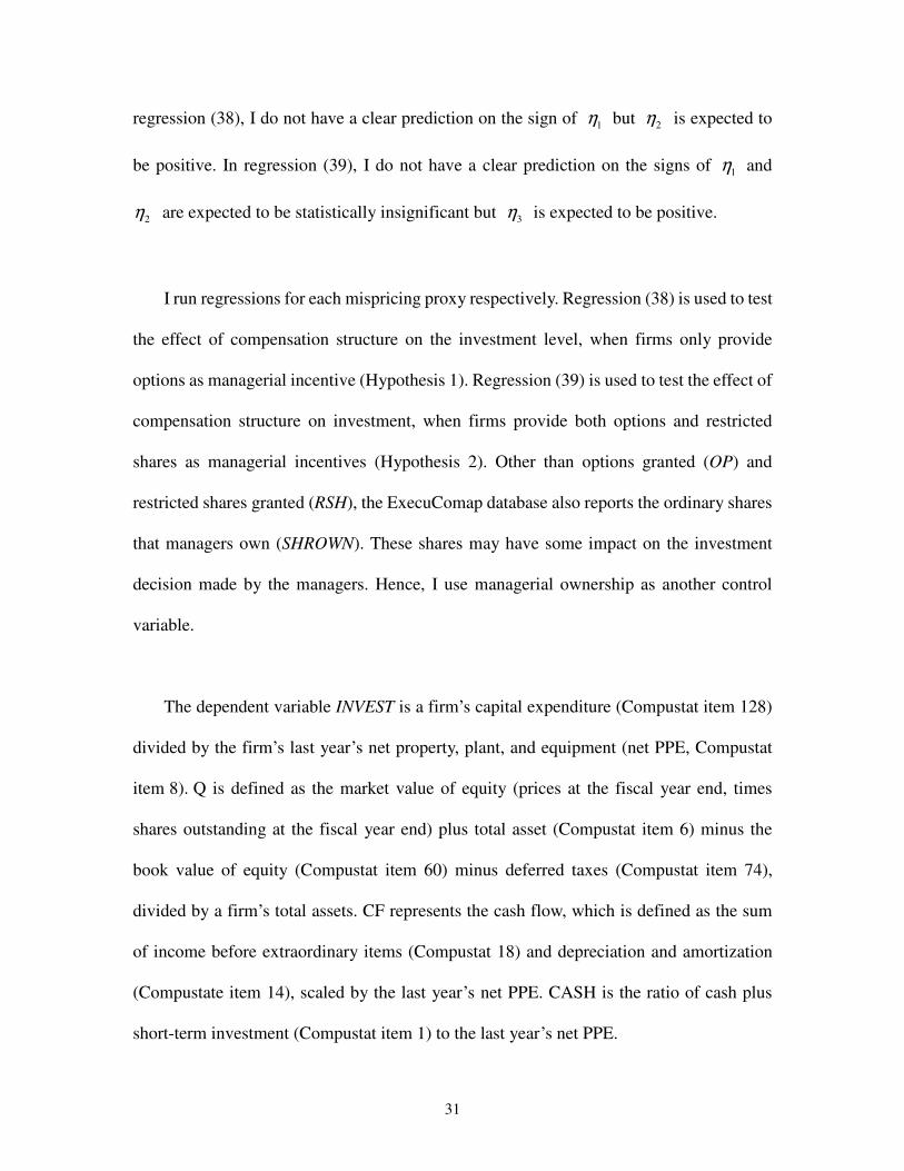
Table 4 reports the correlations between variables for the corresponding samples in Table 3.

Table 4: Executive Compensation and Corporate Investment with Discretionary

Accruals as Mispricing Proxy: Correlations between Variables

47

N Median SD Mean Min 25%th 75%th Max

INVEST 10558 0.24 0.35 0.36 0.03 0.14 0.44 1.88

OP 10558 2.28 2.75 3.03 0.05 0.98 4.20 13.10

Q 10558 1.66 1.62 2.22 0.76 1.21 2.56 9.36

CF 10558 0.39 1.63 0.70 -4.42 0.16 0.91 8.35

CASH 10558 0.38 5.69 2.45 0.00 0.07 1.96 38.04

SHROWN 10558 0.71 6.19 3.28 0.00 0.18 3.05 33.12

TURN 10558 0.11 0.15 0.16 0.02 0.06 0.21 0.74

INVEST 5440 0.19 0.20 0.24 0.03 0.12 0.29 1.88

OP 5440 1.30 1.91 1.88 0.05 0.57 2.50 13.10

RSH 5440 0.11 0.74 0.25 0.00 0.04 0.26 22.96

Q 5440 1.45 1.10 1.80 0.76 1.14 2.05 9.36

CF 5440 0.35 1.12 0.59 -4.42 0.17 0.66 8.35

CASH 5440 0.17 4.94 1.47 0.00 0.05 0.69 38.04

SHROWN 5440 0.32 3.93 1.50 0.00 0.12 0.93 33.12

TURN 5440 0.09 0.10 0.12 0.02 0.06 0.14 0.74

INVEST 8566 0.23 0.31 0.33 0.03 0.14 0.40 1.68

OP 8566 1.10 1.54 1.58 0.03 0.51 2.14 7.82

Q 8566 1.62 1.54 2.15 0.75 1.20 2.41 8.98

CF 8566 0.38 1.52 0.65 -4.29 0.16 0.86 7.71

CASH 8566 0.34 5.27 2.24 0.00 0.06 1.74 36.21

SHROWN 8566 0.39 5.24 2.53 0.00 0.09 2.04 28.68

TURN 8566 0.11 0.15 0.16 0.02 0.06 0.21 0.74

INVEST 3955 0.19 0.19 0.24 0.03 0.12 0.29 1.68

OP 3955 0.62 1.08 0.98 0.03 0.28 1.27 7.82

RSH 3955 0.06 0.63 0.16 0.00 0.02 0.16 20.20

Q 3955 1.44 1.04 1.76 0.75 1.15 1.99 8.98

CF 3955 0.34 1.02 0.56 -4.29 0.17 0.64 7.71

CASH 3955 0.16 4.93 1.41 0.00 0.04 0.60 36.21

SHROWN 3955 0.15 2.88 0.85 0.00 0.05 0.43 28.68

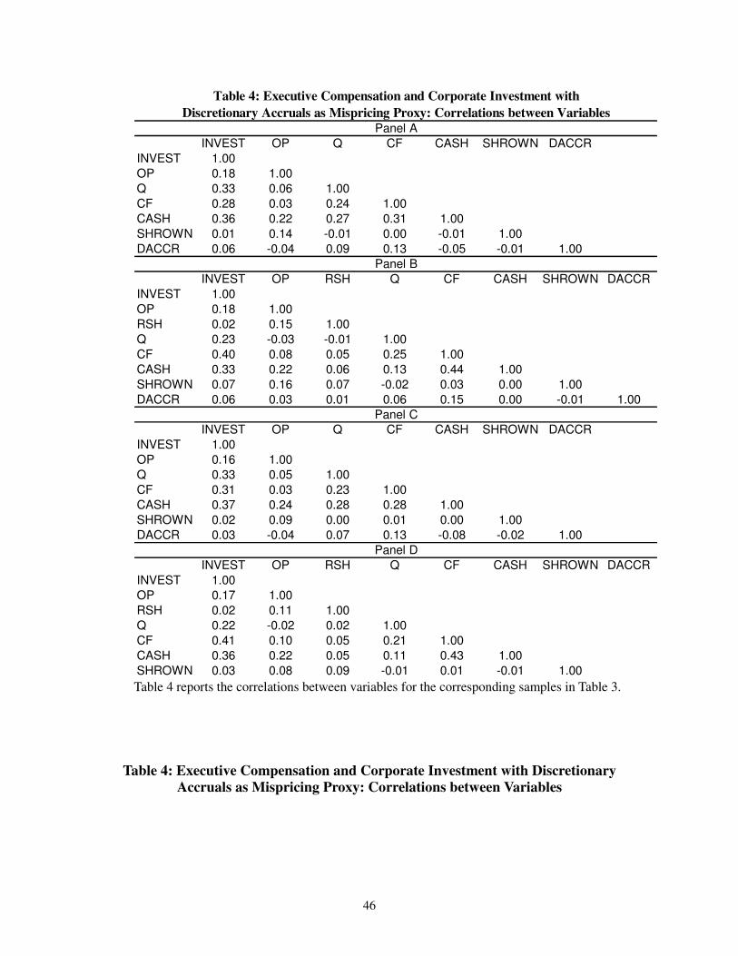
Turnover Ratio as Mispricing Proxy: Sample Summary Statistics

Panel D

Table 5: Executive Compensation and Corporate Investment with Share

Panel A

Panel B

Panel C

Table 5 reports the sample statistics for the regressions of investment on compensation when the

mispricing proxy is share turnover ratio. Panel A is for the sample firms that only provide options

to the top management. Panel B is for the sample firms that provide both options and restricted

shares to the top management. Panel C is for the sample firms that only provide options to the

CEOs. Panel D is for the sample firms that provide both options and restricted shares to the CEOs.

Definitions of the variables can be found in Section 3.3.1.

Table 5: Executive Compensation and Corporate Investment with Share Turnover

Ratio as Mispricing Proxy: Sample Summary Statistics

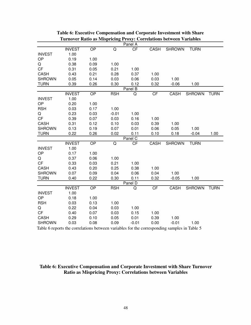
48

INVEST OP Q CF CASH SHROWN TURN

INVEST 1.00

OP 0.19 1.00

Q 0.38 0.09 1.00

CF 0.31 0.05 0.21 1.00

CASH 0.43 0.21 0.28 0.37 1.00

SHROWN 0.05 0.14 0.03 0.06 0.03 1.00

TURN 0.39 0.26 0.30 0.12 0.32 -0.06 1.00

INVEST OP RSH Q CF CASH SHROWN TURN

INVEST 1.00

OP 0.20 1.00

RSH 0.03 0.17 1.00

Q 0.23 0.03 -0.01 1.00

CF 0.39 0.07 0.03 0.16 1.00

CASH 0.31 0.12 0.10 0.03 0.39 1.00

SHROWN 0.13 0.19 0.07 0.01 0.06 0.05 1.00

TURN 0.22 0.26 0.02 0.11 0.10 0.18 -0.04 1.00

INVEST OP Q CF CASH SHROWN TURN

INVEST 1.00

OP 0.17 1.00

Q 0.37 0.06 1.00

CF 0.33 0.03 0.21 1.00

CASH 0.43 0.20 0.25 0.38 1.00

SHROWN 0.07 0.09 0.04 0.06 0.04 1.00

TURN 0.40 0.22 0.30 0.11 0.32 -0.05 1.00

INVEST OP RSH Q CF CASH SHROWN TURN

INVEST 1.00

OP 0.18 1.00

RSH 0.03 0.13 1.00

Q 0.22 0.04 0.03 1.00

CF 0.40 0.07 0.03 0.15 1.00

CASH 0.29 0.10 0.05 0.01 0.39 1.00

SHROWN 0.03 0.08 0.09 -0.01 0.00 -0.01 1.00

Table 6: Executive Compensation and Corporate Investment with Share

Turnover Ratio as Mispricing Proxy: Correlations between VariablesPanel A

Panel B

Panel C

Panel D

Table 6 reports the correlations between variables for the corresponding samples in Table 5

Table 6: Executive Compensation and Corporate Investment with Share Turnover

Ratio as Mispricing Proxy: Correlations between Variables

49

N Median SD Mean Min 25%th 75%th Max

INVEST 8050 0.25 0.35 0.37 0.03 0.15 0.45 1.88

OP 8050 2.35 2.64 3.04 0.06 1.04 4.24 12.33

Q 8050 1.71 1.70 2.31 0.80 1.25 2.67 9.92

CF 8050 0.43 1.70 0.81 -3.88 0.18 0.97 9.29

CASH 8050 0.45 5.78 2.59 0.00 0.07 2.18 37.34

SHROWN 8050 0.74 6.01 3.29 0.00 0.19 3.14 30.47

DISP 8050 -6.08 1.32 -6.07 -9.46 -6.94 -5.21 -2.71

INVEST 4216 0.19 0.20 0.24 0.03 0.12 0.29 1.88

OP 4216 1.35 1.89 1.92 0.06 0.60 2.54 12.33

RSH 4216 0.11 0.50 0.24 0.00 0.04 0.26 13.00

Q 4216 1.47 1.18 1.85 0.80 1.15 2.11 9.92

CF 4216 0.37 1.20 0.63 -3.88 0.17 0.70 9.29

CASH 4216 0.19 4.89 1.52 0.00 0.05 0.77 37.34

SHROWN 4216 0.34 3.58 1.43 0.00 0.12 0.94 30.47

DISP 4216 -6.54 1.20 -6.54 -9.46 -7.29 -5.76 -2.71

INVEST 6614 0.24 0.31 0.34 0.03 0.14 0.42 1.71

OP 6614 1.13 1.46 1.57 0.03 0.53 2.15 7.34

Q 6614 1.67 1.64 2.23 0.80 1.24 2.55 9.67

CF 6614 0.42 1.57 0.76 -3.60 0.18 0.92 8.45

CASH 6614 0.40 5.31 2.36 0.00 0.07 2.01 35.15

SHROWN 6614 0.41 5.17 2.58 0.00 0.09 2.10 26.89

DISP 6614 -6.22 1.30 -6.22 -9.48 -7.07 -5.37 -2.89

INVEST 3077 0.19 0.19 0.24 0.03 0.12 0.29 1.71

OP 3077 0.65 1.08 1.00 0.03 0.29 1.30 7.34

RSH 3077 0.06 0.33 0.14 0.00 0.03 0.15 8.30

Q 3077 1.45 1.14 1.81 0.80 1.15 2.07 9.67

CF 3077 0.35 1.07 0.60 -3.60 0.17 0.67 8.45

CASH 3077 0.17 4.85 1.46 0.00 0.04 0.68 35.15

SHROWN 3077 0.15 2.61 0.79 0.00 0.05 0.41 26.89

Analyst Forecasts as Mispricing Proxy: Sample Summary Statistics

Table 7: Executive Compensation and Corporate Investment with Dispersion of

Panel A

Panel B

Panel C

Panel D

Table 7 reports the sample statistics for the regressions of investment on compensation when the

mispricing proxy is analyst forecast dispersion. Panel A is for the sample firms that only provide

options to the top management. Panel B is for the sample firms that provide options and restricted

shares to the top management. Panel C is for the sample firms that only provide options to the

CEOs. Panel D is for the sample firms that provide options and restricted shares to the CEOs.

Definitions of the variables can be found in Section 3.3.1.

Table 7: Executive Compensation and Corporate Investment with Dispersion of

Analyst Forecasts as Mispricing Proxy: Sample Summary Statistics

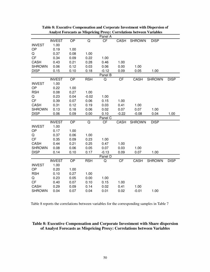
50

INVEST OP Q CF CASH SHROWN DISP

INVEST 1.00

OP 0.19 1.00

Q 0.37 0.08 1.00

CF 0.34 0.09 0.22 1.00

CASH 0.43 0.21 0.28 0.46 1.00

SHROWN 0.06 0.12 0.03 0.06 0.00 1.00

DISP 0.15 0.10 0.18 -0.12 0.09 0.05 1.00

INVEST OP RSH Q CF CASH SHROWN DISP

INVEST 1.00

OP 0.22 1.00

RSH 0.08 0.27 1.00

Q 0.23 0.04 -0.02 1.00

CF 0.39 0.07 0.06 0.15 1.00

CASH 0.31 0.12 0.19 0.03 0.41 1.00

SHROWN 0.13 0.18 0.06 0.02 0.07 0.07 1.00

DISP 0.06 0.09 0.00 0.10 -0.22 -0.08 0.04 1.00

INVEST OP Q CF CASH SHROWN DISP

INVEST 1.00

OP 0.17 1.00

Q 0.37 0.06 1.00

CF 0.35 0.09 0.23 1.00

CASH 0.44 0.21 0.25 0.47 1.00

SHROWN 0.08 0.06 0.05 0.07 0.03 1.00

DISP 0.14 0.10 0.17 -0.13 0.09 0.07 1.00

INVEST OP RSH Q CF CASH SHROWN DISP

INVEST 1.00

OP 0.20 1.00

RSH 0.10 0.27 1.00

Q 0.23 0.05 0.00 1.00

CF 0.40 0.07 0.10 0.15 1.00

CASH 0.29 0.09 0.14 0.02 0.41 1.00

SHROWN 0.04 0.07 0.04 0.01 0.02 -0.01 1.00

Table 8: Executive Compensation and Corporate Investment with Dispersion of

Panel B

Analyst Forecasts as Mispricing Proxy: Correlations between Variables

Panel A

Panel C

Panel D

Table 8 reports the correlations between variables for the corresponding samples in Table 7

Table 8: Executive Compensation and Corporate Investment with Share dispersion

of Analyst Forecasts as Mispricing Proxy: Correlations between Variables

51

N Median SD Mean Min 25%th 75%th Max

INVEST 8583 0.23 0.30 0.33 0.03 0.14 0.41 1.88

OP 8583 2.13 2.72 2.91 0.05 0.91 4.06 13.10

Q 8583 1.62 1.53 2.15 0.76 1.20 2.47 9.36

CF 8583 0.38 1.51 0.69 -4.42 0.17 0.87 8.35

CASH 8583 0.32 5.17 2.16 0.00 0.06 1.65 38.04

SHROWN 8583 0.66 6.26 3.27 0.00 0.17 2.93 33.12

EQISS 8583 0.01 0.74 0.14 -1.85 -0.04 0.10 3.98

INVEST 4568 0.19 0.20 0.24 0.03 0.12 0.29 1.88

OP 4568 1.25 1.86 1.83 0.05 0.56 2.44 13.10

RSH 4568 0.11 0.74 0.25 0.00 0.04 0.26 13.00

Q 4568 1.43 1.06 1.77 0.76 1.14 2.01 9.36

CF 4568 0.34 1.12 0.60 -4.42 0.16 0.65 8.35

CASH 4568 0.16 4.57 1.31 0.00 0.04 0.64 38.04

SHROWN 4568 0.31 3.53 1.37 0.00 0.12 0.89 33.12

EQISS 4568 0.00 0.43 -0.03 -9.46 -0.07 0.02 3.98

INVEST 7024 0.22 0.28 0.31 0.03 0.14 0.38 1.68

OP 7024 1.04 1.52 1.52 0.03 0.46 2.05 7.82

Q 7024 1.60 1.46 2.09 0.75 1.19 2.36 8.98

CF 7024 0.37 1.43 0.66 -4.29 0.17 0.84 7.71

CASH 7024 0.29 4.85 1.99 0.00 0.06 1.49 36.21

SHROWN 7024 0.36 5.27 2.51 0.00 0.08 1.95 28.68

EQISS 7024 0.00 0.64 0.08 -1.86 -0.05 0.08 3.37

INVEST 3343 0.19 0.18 0.23 0.03 0.12 0.28 1.68

OP 3343 0.60 1.05 0.95 0.03 0.27 1.25 7.82

RSH 3343 0.06 0.60 0.16 0.00 0.02 0.16 20.20

Q 3343 1.42 1.01 1.73 0.75 1.14 1.95 8.98

CF 3343 0.33 1.02 0.56 -4.29 0.16 0.62 7.71

CASH 3343 0.14 4.51 1.26 0.00 0.04 0.56 36.21

SHROWN 3343 0.14 2.49 0.77 0.00 0.05 0.40 28.68

Panel C

Panel D

Table 9: Executive Compensation and Corporate Investment with Net Equity

Panel A

Panel B

Issuance as Mispricing Proxy: Sample Summary Statistics

Table 9 reports the sample statistics for the regressions of investment on compensation when the

mispricing proxy is net equity issuance. Panel A is for the sample firms that only provide options

to the top management. Panel B is for the sample firms that provide both options and restricted

shares to the top management. Panel C is for the sample firms that only provide options to the

CEOs. Panel D is for the sample firms that provide both options and restricted shares to the CEOs.

Definitions of the variables can be found in Section 3.3.1.

Table 9: Executive Compensation and Corporate Investment with Net Equity

Issuance as Mispricing Proxy: Sample Summary Statistics

52

INVEST OP Q CF CASH SHROWN EQISS

INVEST 1.00

OP 0.19 1.00

Q 0.34 0.07 1.00

CF 0.32 0.07 0.22 1.00

CASH 0.38 0.21 0.24 0.42 1.00

SHROWN 0.04 0.14 0.02 0.04 0.02 1.00

EQISS 0.33 0.13 0.18 -0.04 0.33 -0.02 1.00

INVEST OP RSH Q CF CASH SHROWN EQISS

INVEST 1.00

OP 0.20 1.00

RSH 0.03 0.19 1.00

Q 0.23 0.01 -0.02 1.00

CF 0.41 0.08 0.03 0.16 1.00

CASH 0.30 0.13 0.12 0.03 0.44 1.00

SHROWN 0.14 0.21 0.09 0.00 0.05 0.05 1.00

EQISS 0.11 0.08 0.06 -0.02 -0.26 -0.02 0.03 1.00

INVEST OP Q CF CASH SHROWN EQISS

INVEST 1.00

OP 0.17 1.00

Q 0.33 0.05 1.00

CF 0.34 0.06 0.21 1.00

CASH 0.39 0.20 0.22 0.44 1.00

SHROWN 0.06 0.08 0.02 0.05 0.03 1.00

EQISS 0.27 0.11 0.14 -0.12 0.26 -0.02 1.00

INVEST OP RSH Q CF CASH SHROWN EQISS

INVEST 1.00

OP 0.17 1.00

RSH 0.03 0.14 1.00

Q 0.22 0.01 0.01 1.00

CF 0.41 0.06 0.04 0.17 1.00

CASH 0.28 0.10 0.07 0.01 0.42 1.00

SHROWN 0.05 0.11 0.13 0.00 0.00 0.00 1.00

EQISS 0.07 0.04 0.05 -0.06 -0.23 -0.04 0.02 1.00

Table 10: Executive Compensation and Corporate Investment with Net Equity

Issuance as Mispricing Proxy: Correlations between Variables

Panel B

Panel C

Panel D

Table 10 reports the correlations between variables for the corresponding samples in Table 9.

Table 10: Executive Compensation and Corporate Investment with Net Equity

Issuance as Mispricing Proxy: Correlations between Variables

53

(1) (2) (3) (4)

OP 0.0016 OP 0.0067 OP 0.0056 OP 0.0032

[0.71] [2.76] [0.75] [1.67]

DACCR 0.0340 TURN 0.4491 DISP-1 0.0068 EQISS 0.0504

[4.27] 8.5600 [1.08] [5.07]

Q-1 0.0492 Q-1 0.0497 Q-1 0.0502 Q-1 0.0397

[15.76] [18.77] [17] [13.81]

CF 0.0351 CF 0.0429 CF 0.0518 CF 0.0395

[8.86] [16.48] [16.18] [12.75]

CASH-1 0.0163 CASH-1 0.0165 CASH-1 0.0178 CASH-1 0.0150

[11.63] [19.54] [17.09] [14.74]

SHROWN -0.0002 SHROWN 0.0011 SHROWN 0.0008 SHROWN -0.0002

[-0.26] [1.41] [0.82] [-0.19]

OP*DACCR -0.0004 OP*TURN -0.0286 OP*DISP-1 0.0006 OP*EQISS 0.0014

[-0.24] [-3.23] [0.49] [0.88]

Firm-year 5411 Firm-year 8859 Firm-year 6584 Firm-year 7061

R square 0.2943 R square 0.4468 R square 0.3656 R square 0.4010

(1) (2) (3) (4)

OP 0.0008 OP 0.0012 OP -0.0028 OP 0.0021

[0.3] [0.4] [-0.25] [0.92]

RSH -0.0044 RSH 0.0007 RSH 0.0471 RSH -0.0004

[-1.42] [0.17] [1.6] [0.11]

DACCR 0.0168 TURN 0.0654 DISP-1 -0.0094 EQISS 0.0904

[2] [1.18] [-1.71] [6.55]

Q-1 0.0305 Q-1 0.0294 Q-1 0.0242 Q-1 0.0316

[8.45] [8.54] [6.66] [8.17]

CF 0.0627 CF 0.0568 CF 0.0734 CF 0.0689

[11.42] [14.43] [13.98] [15.52]

CASH-1 0.0298 CASH-1 0.0143 CASH-1 0.0123 CASH-1 0.0032

[11.49] [11.3] [7.15] [2.13]

SHROWN -0.0004 SHROWN 0.0016 SHROWN 0.0021 SHROWN 0.0007

[-0.3] [1.47] [1.32] [0.58]

OP*DACCR 0.0005 OP*TURN 0.0054 OP*DISP-1 -0.0012 OP*EQISS -0.0057

[0.21] [0.37] [-0.72] [-1.71]

RSH*DACCR -0.0152 RSH*TURN -0.0659 RSH*DISP-1 0.0086 RSH*EQISS -0.0137

[-1.64] [-1.19] [1.98] [-3.79]

Firm-year 3237 Firm-year 4885 Firm-year 3704 Firm-year 4018

R square 0.3349 R square 0.3589 R square 0.3076 R square 0.3729

Panel A

Table 11: Executive Compensation and Corporate Investment (Top Executives)

Panel B

Table 11 reports the results for the sample of top executives. Panel A is for the sample of

managers who only hold options. Panel B is for the sample of managers who hold both options

and restricted shares. In column 1, the mispricing proxy is discretionary accruals. In column 2, the

mispricing proxy is turnover ratio. In column 3, the mispricing proxy is the dispersion of analyst

forecast. In column 4, the mispricing proxy is past net equity issuance. The model specification

can be found in Section 3.3.1.

Table 11: Executive Compensation and Corporate Investment (Top Executives)

54

(1) (2) (3) (4)

OP -0.0046 OP 0.0131 OP 0.0311 OP 0.0085418

[-0.99] [2.66] [1.98] [2.21]

DACCR 0.0156 TURN 0.3803 DISP-1 0.0039 EQISS 0.0607688

[1.72] [6.9] [0.6] [5.26]

Q-1 0.0462 Q-1 0.0473 Q-1 0.0472 Q-1 0.0363091

[13.52] [16.36] [14.83] [11.36]

CF 0.0372 CF 0.0396 CF 0.0535 CF 0.0399153

[7.94] [13.02] [13.93] [11.15]

CASH-1 0.0172 CASH-1 0.0152 CASH-1 0.0199 CASH-1 0.0122764

[10.56] [15.5] [15.56] [10.28]

SHROWN 0.0000 SHROWN 0.0018 SHROWN 0.0010 SHROWN -0.0007751

[0] [1.46] [0.68] [-0.58]

OP*DACCR 0.0030 OP*TURN -0.0425 OP*DISP-1 0.0033 OP*EQISS -0.0035611

[0.95] [-2.41] [1.31] [-1.11]

Firm-year 4501 Firm-year 6975 Firm-year 5239 Firm-year 5608

R square 0.2967 R square 0.4175 R square 0.3590 R square 0.3780

(1) (2) (3) (4)

OP -0.0037 OP 0.0025 OP -0.0205 OP -0.0015049

[-0.74] [0.43] [-0.84] [-0.29]

RSH -0.0051 RSH -0.0007 RSH 0.3167 RSH -0.003032

[-1.31] [-0.11] [3.03] [-0.47]

DACCR 0.0312 TURN 0.2395 DISP-1 -0.0112 EQISS 0.0458068

[3.35] [3.68] [-1.88] [2.44]

Q-1 0.0341 Q-1 0.0284 Q-1 0.0218 Q-1 0.0342061

[8.06] [7.4] [5.46] [7.62]

CF 0.0726 CF 0.0519 CF 0.0692 CF 0.0534596

[11.54] [11.54] [10.68] [10.12]

CASH-1 0.0186 CASH-1 0.0110 CASH-1 0.0114 CASH-1 0.0032424

[6.18] [7.44] [5.45] [1.82]

SHROWN -0.0006 SHROWN -0.0006 SHROWN -0.0011 SHROWN 0.0008422

[-0.29] [-0.29] [-0.41] [0.34]

OP*DACCR -0.0010 OP*TURN -0.0371 OP*DISP-1 -0.0042 OP*EQISS 0.0076947

[-0.21] [-1.41] [-1.2] [0.64]

RSH*DACCR -0.0496 RSH*TURN -0.0690 RSH*DISP-1 0.0474 RSH*EQISS -0.0204789

[-2.7] [-0.67] [3.18] [-2.2]

Firm-year 2289 Firm-year 3447 Firm-year 2624 Firm-year 2846

R square 0.3619 R square 0.3533 R square 0.3153 R square 0.3361

Panel B

Table 12: Executive Compensation and Corporate Investment (CEOs)

Panel A

Table 12 reports the results for the sample of CEOs. Panel A is the result for the sample of

managers who only hold options. Panel B is the result for the sample of managers who hold both

options and restricted shares. In column 1, the mispricing proxy is discretionary accruals. In

column 2, the mispricing proxy is turnover ratio. In column 3, the mispricing proxy is the

dispersion of analyst forecast. In column 4, the mispricing proxy is past net equity issuance. The

model specification can be found in Section 3.3.1.

Table 12: Executive Compensation and Corporate Investment (CEOs)

55

(1) (2) (3) (4)

OP -0.0015 OP 0.0072 OP 0.0061 OP 0.0047

[-0.58] [2.7] [0.7] [2.16]

DACCR 0.0286 TURN 0.3600 DISP-1 0.0089 EQISS 0.0173

[3.19] [6.22] [1.24] [1.47]

Q-1 0.0481 Q-1 0.0468 Q-1 0.0454 Q-1 0.0417

[13.16] [15.56] [13.56] [12.18]

CF 0.0258 CF 0.0409 CF 0.0525 CF 0.0357

[5.43] [13.65] [13.83] [10.11]

CASH-1 0.0149 CASH-1 0.0148 CASH-1 0.0157 CASH-1 0.0124

[8.7] [13.86] [11.77] [9.8]

SHROWN 0.0009 SHROWN 0.0008 SHROWN 0.0000 SHROWN -0.0004

[0.92] [0.97] [0] [-0.47]

OP*DACCR 0.0007 OP*TURN -0.0144 OP*DISP-1 0.0001 OP*EQISS 0.0063

[0.42] [-1.45] [0.1] [3.39]

Q-2 0.0002 Q-2 0.0004 Q-2 0.0040 Q-2 0.0040

[0.05] [0.14] [1.25] [1.25]

Firm-year 4353 Firm-year 7314 Firm-year 5285 Firm-year 5735

R square 0.2681 R square 0.4426 R square 0.3840 R square 0.3670

(1) (2) (3) (4)

OP 0.0017 OP 0.0018 OP 0.0046 OP 0.0020

[0.64] [0.54] [0.36] [0.81]

RSH -0.0050 RSH -0.0005 RSH 0.0479 RSH 0.0002

[-1.58] [-0.11] [0.86] [0.04]

DACCR 0.0268 TURN 0.0835 DISP-1 -0.0122 DISP 0.0956

[2.85] [1.43] [-1.92] [6.34]

Q-1 0.0320 Q-1 0.0284 Q-1 0.0214 Q-1 0.0400

[7.35] [6.89] [4.82] [8.71]

CF 0.0582 CF 0.0513 CF 0.0696 CF 0.0653

[9.59] [12.12] [11.64] [13.69]

CASH-1 0.0183 CASH-1 0.0158 CASH-1 0.0132 CASH-1 0.0028

[6.32] [11.37] [6.42] [1.69]

SHROWN -0.0012 SHROWN 0.0011 SHROWN 0.0015 SHROWN -0.0001

[-0.9] [0.96] [0.84] [-0.08]

OP*DACCR 0.0020 OP*TURN 0.0053 OP*DISP-1 -0.0004 OP*EQISS -0.0113

[0.7] [0.34] [-0.23] [-3.1]

RSH*DACCR -0.0387 RSH*TURN -0.0280 RSH*DISP-1 0.0075 RSH*EQISS -0.0121

[-3.19] [-0.41] [0.9] [-2.81]

Q-2 0.0011 Q-2 0.0045 Q-2 0.0068 Q-2 -0.0089

[0.27] [1.16] [1.61] [-2.08]

Firm-year 2785 Firm-year 4299 Firm-year 3193 Firm-year 3447

R square 0.3049 R square 0.3461 R square 0.3378 R square 0.3387

Panel A

Table 13: Executive Compensation and Corporate Investment (Top Executives) with Lags of Q

Panel B

Table 13 reports the results for the sample of top executives by adding two lags of Q as control

variables.

Table 13: Executive Compensation and Corporate Investment (Top Executives) with

Lags of Q

56

(1) (2) (3) (4)

OP -0.0103 OP 0.0104 OP 0.0455 OP 0.0089

[-1.96] [1.9] [2.45] [1.99]

DACCR 0.0184 TURN 0.2854 DISP-1 -0.0075 EQISS 0.0453

[1.84] [4.76] [-103] [3.18]

Q-1 0.0446 Q-1 0.0461 Q-1 0.0443 Q-1 0.0385

[11.42] [13.74] [12.09] [10.11]

CF 0.0346 CF 0.0381 CF 0.0605 CF 0.0434

[6.33] [10.74] [12.67] [10.46]

CASH-1 0.0167 CASH-1 0.0142 CASH-1 0.0166 CASH-1 0.0091

[8.33] [11.62] [10.25] [6.21]

SHROWN -0.0005 SHROWN 0.0007 SHROWN 0.0010 SHROWN -0.0016

[-0.26] [0.5] [0.61] [-1.01]

OP*DACCR -0.0021 OP*TURN -0.0244 OP*DISP-1 0.0052 OP*EQISS 0.0055

[-0.6] [-1.26] [1.74] [1.36]

Q-2 0.0058 Q-2 0.0013 Q-2 0.0052 Q-2 -0.0011

[1.58] [0.42] [0.46] [-0.31]

Firm-year 3522 Firm-year 5568 Firm-year 4071 Firm-year 4394

R square 0.3199 R square 0.4312 R square 0.3802 R square 0.3579

(1) (2) (3) (4)

OP -0.0121 OP -0.0022 OP -0.0203 OP 0.0014

[-2.27] [-0.35] [-0.76] [0.26]

RSH -0.0042 RSH -0.0087 RSH 0.1490 RSH 0.0083

[-1.01] [-1.34] [1.25] [0.46]

DACCR 0.0390 TURN 0.1408 DISP-1 -0.0101 DISP 0.0249

[3.82] [2.11] [-1.56] [1.28]

Q-1 0.0290 Q-1 0.0236 Q-1 0.0156 Q-1 0.0335

[6.04] [5.38] [3.31] [6.44]

CF 0.0527 CF 0.0406 CF 0.0610 CF 0.0481

[7.08] [8.54] [8.3] [8.45]

CASH-1 0.0118 CASH-1 0.0122 CASH-1 0.0054 CASH-1 0.0028

[3.51] [6.97] [2.3] [1.35]

SHROWN -0.0004 SHROWN -0.0020 SHROWN -0.0031 SHROWN 0.0001

[-0.16] [-0.91] [-1.09] [0.05]

OP*DACCR -0.0030 OP*TURN -0.0424 OP*DISP-1 -0.0035 OP*EQISS 0.0061

[-0.55] [-1.54] [-0.92] [0.49]

RSH*DACCR -0.0484 RSH*TURN 0.0922 RSH*DISP-1 0.0261 RSH*EQISS 0.0714

[-2.6] [0.88] [1.52] [2.48]

Q-2 0.0061 Q-2 0.0108 Q-2 0.0138 Q-2 0.0008

[1.3] [2.53] [2.93] [0.15]

Firm-year 1921 Firm-year 2953 Firm-year 2200 Firm-year 2384

R square 0.3154 R square 0.2705 R square 0.2784 R square 0.3146

Table 14: Executive Compensation and Corporate Investment (CEOs) with Lags of Q

Panel A

Panel B

Table 14 reports the results for the sample of top executives by adding three lags of Q as control

variables.

Table 14: Executive Compensation and Corporate Investment (CEOs) with Lags of

Q

57

(1) (2) (3) (4)

OP 0.0007 OP 0.0079 OP 0.0080 OP 0.0039

[0.34] [3.05] [ 0.86] [2.03]

DACCR 0.0382 TURN 0.4340 DISP -0.0018 EQISS 0.0348

[4.79] [7.08] [-0.21] [2.88]

DACCR-1 0.0376 TURN-1 0.0063 DISP-1 0.0235 EQISS-1 0.0230

[4.67] [0.10] [ 2.81] [1.96 ]

Q 0.0475 Q 0.0497 Q 0.0450 Q 0.0398

[15.15] [18.74] [13.89] [13.81]

CF 0.0333 CF 0.0429 CF 0.0503 CF 0.0395

[8.38] [16.48] [13.28] [12.75]

CASH 0.0164 CASH 0.0165 CASH 0.0160 CASH 0.0150

[11.71] [19.54] [12.14] [14.74]

SHROWN 0.0000 SHROWN 0.0011 SHROWN -0.0001 SHROWN -0.0002

[-0.05] [1.37] [ -0.09] [-0.21]

OP*DACCR -0.0007 OP*TURN -0.0208 OP*DISP 0.0004 OP*EQISS 0.0051

[-0.47] [-1.95] [0.18] [2.59]

OP*DACCR-1 -0.0038 OP*TURN-1 -0.0148 OP*DISP-1 0.0002 OP*EQISS-1 -0.0060

[-2.63] [-1.39] [0.12] [-3.16]

Firm-year 5411 Firm-year 8859 Firm-year 5285 Firm-year 7061

R square 0.2836 R square 0.4435 R square 0.3870 R square 0.3981

(1) (2) (3) (4)

OP 0.0004 OP -0.0011 OP 0.0195 OP 0.0024

[0.15] [-0.36] [1.43] [0.92]

RSH -0.0046 RSH -0.0013 RSH 0.0586 RSH -0.0003

[-1.50] [-0.28] [1.00] [-0.07]

DACCR 0.0181 TURN 0.1050 DISP -0.0088 EQISS 0.0760

[2.15] [1.53] [-1.16] [4.23]

DACCR-1 0.0134 TURN-1 -0.0607 DISP-1 -0.0053 EQISS-1 0.0198

[1.59] [-0.81] [-0.73] [1.23]

Q 0.0302 Q 0.0294 Q 0.0235 Q 0.0303

[8.33] [8.54] [ 5.86] [8.08]

CF 0.0635 CF 0.0568 CF 0.0708 CF 0.0689

[11.42] [14.43] [11.81] [15.52]

CASH 0.0298 CASH 0.0144 CASH 0.0130 CASH 0.0032

[11.22] [10.99] [ 6.39] [1.98]

SHROWN -0.0004 SHROWN 0.0016 SHROWN 0.0013 SHROWN 0.0007

[-0.36] [1.47] [0.74] [0.58]

OP*DACCR -0.0001 OP*TURN 0.0054 OP*DISP -0.0054 OP*EQISS -0.0043

[-0.05] [0.37] [-2.22] [-1.00]

OP*DACCR-1 -0.0047 OP*TURN-1 0.0335 OP*DISP-1 0.0073 OP*EQISS-1 -0.0009

[-1.68] [1.72] [3.17] [-0.22]

RSH*DACCR -0.0155 RSH*TURN -0.0971 RSH*DISP 0.0276 RSH*EQISS -0.0148

[-1.48] [-1.59] [2.24] [-3.43]

RSH*DACCR-1 0.0205 RSH*TURN-1 0.0811 RSH*DISP-1 -0.0190 RSH*EQISS-1 0.0030

[1.75] [1.30] [-2.70] [0.54]

Firm-year 3237 Firm-year 4885 Firm-year 3193 Firm-year 4018

Panel A

with Lags of Mispricing Proxies

Panel B

Table 15: Executive Compensation and Corporate Investment (Top Executives)

Table 15 reports the results for the sample of top executives by adding one lag of mispricing

proxies as control variables.

Table 15: Executive Compensation and Corporate Investment (Top Executives) with

Lags of Mispricing Proxy

58

(1) (2) (3) (4)

OP -0.0060 OP 0.0157 OP 0.0532 OP 0.0096

[-1.29] [3.01] [2.74] [2.48]

DACCR 0.0233 TURN 0.3574 DISP -0.0104 EQISS 0.0433

[2.52] [5.6] [-1.2] [3.20]

DACCR-1 0.0372 TURN-1 0.0077 DISP-1 0.0153 EQISS-1 0.0271

[4.04] [0.12] [1.84] [2.18]

Q 0.0445 Q 0.0473 Q 0.0433 Q 0.0363

[12.96] [16.36] [12.2] [11.53]

CF 0.0359 CF 0.0392 CF 0.0588 CF 0.0368

[7.68] [12.87] [12.38] [11.53]

CASH 0.0174 CASH 0.0155 CASH 0.0166 CASH 0.0128

[10.73] [15.68] [10.46] [10.21]

SHROWN 0.0000 SHROWN 0.0018 SHROWN 0.0010 SHROWN -0.0010

[0.01] [1.44] [0.60] [-0.74]

OP*DACCR 0.0015 OP*TURN -0.0222 OP*DISP 0.0024 OP*EQISS 0.0024

[0.48] [-1.03] [0.62] [0.64]

OP*DACCR-1 -0.0074 OP*TURN-1 -0.0363 OP*DISP-1 0.0044 OP*EQISS-1 -0.0105

[-2.40] [-1.68] [1.21] [-2.90]

Firm-year 4501 Firm-year 6975 Firm-year 4071 Firm-year 5608

R square 0.2884 R square 0.4128 R square 0.3829 R square 0.3753

(1) (2) (3) (4)

OP -0.0044 OP -0.0035 OP -0.0182 OP -0.0027

[-0.87] [-0.57] [-0.63] [-0.52]

RSH -0.0047 RSH 0.0007 RSH 0.2252 RSH -0.0034

[-1.21] [0.11] [1.76] [-0.52]

DACCR 0.0318 TURN 0.2605 DISP -0.0063 EQISS 0.0427

[3.27] [3.34] [-0.82] [2.06]

DACCR-1 0.0111 TURN-1 0.0718 DISP-1 -0.0116 EQISS-1 0.0179

[1.19] [0.88] [-1.57] [0.97]

Q 0.0333 Q 0.0286 Q 0.0223 Q 0.0347

[7.84] [7.49] [5.27] [7.75]

CF 0.0718 CF 0.0516 CF 0.0627 CF 0.0531

[11.02] [11.55] [8.52] [10.03]

CASH 0.0182 CASH 0.0100 CASH 0.0059 CASH 0.0035

[5.78] [6.78] [2.54] [1.97]

SHROWN -0.0005 SHROWN -0.0006 SHROWN -0.0032 SHROWN 0.0008

[-0.28] [-0.31] [-1.1] [0.33]

OP*DACCR -0.0004 OP*TURN -0.1204 OP*DISP -0.0045 OP*EQISS 0.0115

[-0.07] [-3.46] [-0.98] [0.91]

OP*DACCR-1 -0.0018 OP*TURN-1 0.1466 OP*DISP-1 0.0013 OP*EQISS-1 -0.0188

[-0.35] [3.88] [0.3] [-1.95]

RSH*DACCR -0.0485 RSH*TURN 0.0068 RSH*DISP 0.0056 RSH*EQISS -0.0497

[-2.64] [0.06] [0.22] [-3.84]

RSH*DACCR-1 0.0156 RSH*TURN-1 -0.1224 RSH*DISP-1 0.0319 RSH*EQISS-1 0.0343

[0.88] [-1.17] [1.30] [3.25]

Firm-year 2289 Firm-year 3447 Firm-year 2200 Firm-year 2846

Panel A

Panel B

Table 16: Executive Compensation and Corporate Investment (CEOs)

with Lags of Mispricing Proxies

Table 16 reports the results for the sample of CEOs by adding one lag of mispricing proxies as

control variables.

Table 16: Executive Compensation and Corporate Investment (CEOs) with Lags of

Mispricing Proxy

59

REFERENCES

Aggarwal R. K., and A. A. Samwick (1999). “Empire-builders and shirkers: Investment,

firm performance, and managerial incentives”. NBER working paper,

http://www.nber.org/papers/w7335.

Agrawal, A., and G. N. Mandelker. (1987). “Managerial incentives and corporate

investment and financing decisions”. Journal of Finance, 42, 823-837.

Baker, M., and J. Wurgler. (2006). “Investor sentiment and the cross-section of stock

returns”. Journal of Finance, 61, 1645-1680.

Baker, M., and J.C Stein. (2004). “Market liquidity as a sentiment indicator”. Journal of

Financial markets 7, 271-299.

Baker, M., J. C. Stein and J. Wurgler. (2003), “When does the market matter? Stock

prices and the investment of equity-dependent firms”. The Quarterly Journal of

Economics, August, 271-299.

Blanchard O., C. Rhee, and L. Summers (1993), “The stock market, profit, and

investment”. Quarterly Journal of Economics, 108, 115-136.

Chan, K, L.K.C, Chan, N. Jegadeesh, and J. Lakonishok (2006), “Earnings quality and

stock returns”. Journal of Business, 79, 1041-1082.

Chang, X., H. K. Tam, T. J. Tan, and G. Wong. (2007) “The Real Impact of Stock Market

Mispricing - Evidence from Australia”, Pacific Basin Finance Journal, forthcoming.

Daniel, K., and S. Titman. (2006). “Market reactions to tangible and intangible

information”. Journal of Finance, 65, 1605-1643.

Datta, S., M. Iskandar-Datta, and K. Raman. (2001). “Executive compensation and

corporate acquisition decisions”. Journal of Finance, 56, 2299-2336.

DeLong, J. B., A. Shleifer, L. H. Summers, and R. J. Waldmann. (1990). “Noise trader

risk in financial markets”. Journal of Political Economy, 98, 703-738

Diether K.B, C.J. Malloy, and A. Scherbina (2002). “Differences of opinion and the

Cross Section of stock returns”. Journal of Finance, 57, 2113-2141.

Dong, M., D.A. Hirshleifer, and S.H. Teoh. (2007). “Stock market misvaluation and

corporate investment”. Available at SSRN: http://ssrn.com/abstract=972765

Gilchrist S., C. P. Himmelberg, and G. Huberman (2004), “Do stock price influence

coporate investment”? Federal Reserve Bank of New York Staff Reports, no. 177.

Goyal V. K, and T. Yamada (2004), “Asset prices, financial constraints, and investment

60

evidence from Japan”. The Journal of Business, 77, 175–199.

Lee, C.M.C, and B. Swaminathan. (2000). “Price momentum and trading volume”.

Journal of Finance, 55, 2017-2069.

Mork, R., A. Shlefier, and R. W. Vishny. (1990). “The stock market and investment: Is

the market a sideshow”? Brookings Papers on Economic Activity, 1990, 157-215.

Murphy, K. (1999). “Executive compensation” in Orley Ashenfelter and David Card

(eds.), Handbook of Labor Economics, Vol. 3b, Elsevier Science North Holland (1999),

Chapter 38: 2485-2563.

Polk . C. and P. Sapienza. (2006). “The stock market and corporate investment: A test of

catering theory”. Review of Financial Studies, forthcoming.

Ronnie Sadka, and Anna Scherbina (2007), “Analyst disagreement, mispricing and

liquidity”. Journal of Finance, 62, 2367-2404.

Stein, J. C. (1996). “Rational capital budgeting in an irrational world”. Journal of

Business, 69, 429-455.