Investigation of the Stimulated Brillouin Scattering (SBS ... · Investigation of the Stimulated...
138
Investigation of the Stimulated Brillouin Scattering (SBS) Gain Enhancement in Silicon Nano-Waveguides and Applications Von der Fakultät für Elektrotechnik, Informationstechnik, Physik der Technischen Universität Carolo-Wilhelmina zu Braunschweig zur Erlangung des Grades eines Doktors der Ingenieurwissenschaften (Dr.-Ing.) genehmigte Dissertation von Hassanain Majeed Al-Taiy (Irak, Bagdad, University of Information Technology and Communications) aus Irak, Bagdad eingereicht am: 06.10.2016 mündliche Prüfung am: 17.01.2017 1. Referent: Prof. Dr. rer. nat. Thomas Schneider 2. Referent: Jun.-Prof. Dr. Kambiz Jamshidi Druckjahr: 2017
Transcript of Investigation of the Stimulated Brillouin Scattering (SBS ... · Investigation of the Stimulated...
Investigation of the Stimulated Brillouin Scattering (SBS) GainEnhancement in Silicon Nano-Waveguides and Applications
Von der Fakultät für Elektrotechnik, Informationstechnik, Physikder Technischen Universität Carolo-Wilhelmina zu Braunschweig
zur Erlangung des Grades eines Doktorsder Ingenieurwissenschaften (Dr.-Ing.)
genehmigte Dissertation
von Hassanain Majeed Al-Taiy
(Irak, Bagdad, University of Information Technology and Communications)
aus Irak, Bagdad
eingereicht am: 06.10.2016
mündliche Prüfung am: 17.01.2017
1. Referent: Prof. Dr. rer. nat. Thomas Schneider2. Referent: Jun.-Prof. Dr. Kambiz Jamshidi
Druckjahr: 2017

This work was carried out under the supervision of Prof. Dr. rer. nat.
Thomas Schneider, Faculty of Elektrotechnik Engineering, Technischen
Universität Carolo-Wilhelmina zu Braunschweig

Acknowledgment
First of all I want thank my God for saving me and offering me the chance to studyin Germany. Great thanks go to my parents in Baghdad for their praying and encourage-ment. Special thanks go to my family, Shaima’a, Mohammed, Faris and Nora for theirsupport, understanding and encouragement.
Deeply heart thanks go to my supervisor Prof. Thomas Schneider for his continu-ous support and encouragement. I am grateful to Mr. Stefan Preußler for his supportthrough the practical and the writing parts of the study.
Great thanks for Mr. Kambiz Jamshidi for helping me during the organization ofPh.D. letter of acceptance with the supervisor and traveling process from Baghdad toLeipzig.
Special thanks to Mr. Jens Klinger and Norman Wenzel from the Hochschule fürTelekommunikation Leipzig for their support.
I want to acknowledge the Iraqi government: University of Information Technologyand Communications for their financial support and encouragement.
Thanks for Mr. Kevin Leavey for reading my thesis and giving his comments andsuggestions.
Last but not least I want to present this work to the soul of my sister Suad MajeedAl-Taiy for her previous support and encouragement during my B.Sc. and M.Sc. inBaghdad.
iii


Contents
Acknowledgment iii
Glossary ix
Abstract xiii
Kurzfassung xv
1 Introduction 1
1.1 Overview and Motivation . . . . . . . . . . . . . . . . . . . . . . . . . . . 1
1.2 Thesis Outline . . . . . . . . . . . . . . . . . . . . . . . . . . . . . . . . . 5
2 Stimulated Brillouin Scattering 7
2.1 Introduction . . . . . . . . . . . . . . . . . . . . . . . . . . . . . . . . . . . 7
2.2 Linear and Non-Linear Optical Effects . . . . . . . . . . . . . . . . . . . . 8
2.2.1 Linear Effects . . . . . . . . . . . . . . . . . . . . . . . . . . . . . . 10
2.2.2 Non-Linear Effects . . . . . . . . . . . . . . . . . . . . . . . . . . . 14
2.3 Brillouin Scattering Physics . . . . . . . . . . . . . . . . . . . . . . . . . . 17
2.4 Spontaneous and Stimulated Brillouin Scattering . . . . . . . . . . . . . . 20
2.5 Mathematical Description of SBS . . . . . . . . . . . . . . . . . . . . . . . 23
2.6 Brillouin Scattering Factors . . . . . . . . . . . . . . . . . . . . . . . . . . 29
2.6.1 The Brillouin Gain . . . . . . . . . . . . . . . . . . . . . . . . . . . 29
2.7 Pump Depletion Effects in SBS . . . . . . . . . . . . . . . . . . . . . . . . 31
2.8 Summary . . . . . . . . . . . . . . . . . . . . . . . . . . . . . . . . . . . . 34
3 SBS Gain Enhancement Based on Integrated Silicon Photonics 37
3.1 Introduction . . . . . . . . . . . . . . . . . . . . . . . . . . . . . . . . . . . 37
3.2 Silicon Crystalline Structure . . . . . . . . . . . . . . . . . . . . . . . . . . 38
3.2.1 Silicon Lattice . . . . . . . . . . . . . . . . . . . . . . . . . . . . . 38
3.2.2 Silicon Photo-Elastic Tensor . . . . . . . . . . . . . . . . . . . . . . 40
3.3 Two-Photon Absorption (TPA) in Silicon . . . . . . . . . . . . . . . . . . 42
3.4 Electrostriction Forces . . . . . . . . . . . . . . . . . . . . . . . . . . . . . 43
3.5 Radiation Forces . . . . . . . . . . . . . . . . . . . . . . . . . . . . . . . . 46
3.6 Simulation Method . . . . . . . . . . . . . . . . . . . . . . . . . . . . . . . 47
3.7 220x450 nm Silicon Waveguide . . . . . . . . . . . . . . . . . . . . . . . . 49
3.8 Simulation Results . . . . . . . . . . . . . . . . . . . . . . . . . . . . . . . 50
v

3.8.1 Strip: Air Cladding Waveguide . . . . . . . . . . . . . . . . . . . . 50
3.8.2 Strip Waveguide with Silica Cladding . . . . . . . . . . . . . . . . 54
3.8.3 Rib Waveguide with Air Cladding . . . . . . . . . . . . . . . . . . 56
3.8.4 Rib Waveguide with Silica Cladding . . . . . . . . . . . . . . . . . 61
3.9 Discussion and Concluding Remarks . . . . . . . . . . . . . . . . . . . . . 64
3.10 Suggested Experimental Setup . . . . . . . . . . . . . . . . . . . . . . . . 66
3.11 Summary . . . . . . . . . . . . . . . . . . . . . . . . . . . . . . . . . . . . 67
4 Extraction of High Quality Single Laser Lines 69
4.1 Introduction . . . . . . . . . . . . . . . . . . . . . . . . . . . . . . . . . . . 69
4.2 Optical Frequency Combs . . . . . . . . . . . . . . . . . . . . . . . . . . . 71
4.3 Polarization Pulling-Assisted SBS . . . . . . . . . . . . . . . . . . . . . . . 74
4.4 Laser Linewidth Measurement Techniques . . . . . . . . . . . . . . . . . . 78
4.4.1 Heterodyning with a Local Oscillator . . . . . . . . . . . . . . . . . 78
4.4.2 Delayed Self-Heterodyne . . . . . . . . . . . . . . . . . . . . . . . . 79
4.4.3 Delayed Self-Homodyne (Measurement at the Base Band) . . . . . 80
4.5 Experimental Setup and Results . . . . . . . . . . . . . . . . . . . . . . . 81
4.6 Summary . . . . . . . . . . . . . . . . . . . . . . . . . . . . . . . . . . . . 88
5 High Quality Millimeter Wave Generation 91
5.1 Introduction . . . . . . . . . . . . . . . . . . . . . . . . . . . . . . . . . . . 91
5.2 Millimeter-Wave Generation by Mixing Two Optical Waves . . . . . . . . 93
5.3 Millimeter-Wave Generation and Stabilization . . . . . . . . . . . . . . . . 95
5.3.1 Software Approach . . . . . . . . . . . . . . . . . . . . . . . . . . . 96
5.3.2 Analog Circuit Approach . . . . . . . . . . . . . . . . . . . . . . . 97
5.4 Experimental Setup and Results . . . . . . . . . . . . . . . . . . . . . . . 98
5.5 Discussion and Concluding Remarks . . . . . . . . . . . . . . . . . . . . . 102
5.6 Summary . . . . . . . . . . . . . . . . . . . . . . . . . . . . . . . . . . . . 103
6 Conclusions and Outlook 105
Conclusions . . . . . . . . . . . . . . . . . . . . . . . . . . . . . . . . . . . . . . 105
Outlook . . . . . . . . . . . . . . . . . . . . . . . . . . . . . . . . . . . . . . . . 107
References 109
List of Publications 119
Index 121
vi

List of Figures
2.1 Linear and non-linear interaction effects performance . . . . . . . . . . . . 8
2.2 Energy level diagrams illustrate the possible single photon dipole . . . . . 15
2.3 Brillouin scattering process illustration at medium density fluctuations . . 18
2.4 Illustration of the up-shifted and down-shifted scattered wave frequencies 19
2.5 Isosceles triangle illustrates the wave vectors diagram of the pump . . . . 19
2.6 Schematic representation of the SBS process. . . . . . . . . . . . . . . . . 22
2.7 Effective optical fiber length versus the real optical fiber length . . . . . . 23
2.8 Stokes wave powers at the input of the optical fiber . . . . . . . . . . . . . 29
2.9 Brillouin gain Lorentzian distribution against frequency shift . . . . . . . 30
2.10 Pump and Stokes waves power behavior against optical fiber length . . . . 32
2.11 SBS process illustration with predefined boundary values . . . . . . . . . 34
3.1 Arbitrary three dimensional unit cell. . . . . . . . . . . . . . . . . . . . . . 39
3.2 Silicon unite cell with lattice plane (010). . . . . . . . . . . . . . . . . . . 40
3.3 Indirect band gap illustration of silicon. . . . . . . . . . . . . . . . . . . . 42
3.4 Strip SOI Waveguide . . . . . . . . . . . . . . . . . . . . . . . . . . . . . . 48
3.5 Rib SOI Waveguide . . . . . . . . . . . . . . . . . . . . . . . . . . . . . . . 49
3.6 Normalized electric field of a strip SOI waveguide with air cladding. . . . 51
3.7 FSBS gain profile of a strip air cladding SOI waveguide . . . . . . . . . . 52
3.8 Elastic mode at 12.988 GHz on the FSBS strip air cladding SOI . . . . . 53
3.9 BSBS gain profile of strip air cladding waveguide . . . . . . . . . . . . . . 53
3.10 Elastic mode for the gain at 13.039 GHz in the FSBS strip waveguide . . 54
3.11 FSBS gain profile of a strip waveguide with silica cladding. . . . . . . . . 55
3.12 Elastic mode for the gain at 12.988 GHz in FSBS strip waveguide . . . . . 55
3.13 BSBS gain profile of a strip SOI waveguide with silica cladding. . . . . . . 56
3.14 Elastic mode for the gain at 12.9 GHz in the BSBS strip waveguide . . . . 57
3.15 Normalized electric field of rib air cladding waveguide . . . . . . . . . . . 58
3.16 Normalized electric field of rib air cladding waveguide: transparent . . . . 58
3.17 FSBS gain profile of a rib SOI waveguide with air cladding. . . . . . . . . 59
3.18 Elastic mode at 12.85 GHz of the FSBS rib air cladding SOI waveguide . 59
3.19 BSBS gain profile of a rib SOI waveguide with air cladding. . . . . . . . . 60
3.20 Elastic mode for the gain at 12.94 GHz in the BSBS rib SOI waveguide . 61
3.21 FSBS gain profile of a rib SOI waveguide with silica cladding. . . . . . . . 62
3.22 Excited elastic mode at 12.94 GHz in the FSBS rib SOI waveguide. . . . . 62
3.23 Asymmetric excited elastic mode at 13.048 GHz in FSBS rib SOI waveguide 63
3.24 BSBS gain profile of a rib SOI waveguide with silica cladding. . . . . . . . 63

3.25 Excited elastic mode at 12.9533 GHz in the BSBS rib SOI waveguide . . . 643.26 Suggested experimental setup for SBS gain measurement of SOI waveguide 67
4.1 Pulse train composition by adding three different frequency waves . . . . 714.2 Simulated 100 phase unlocked laser modes. . . . . . . . . . . . . . . . . . 734.3 Simulated 10 phase locked laser modes. . . . . . . . . . . . . . . . . . . . 744.4 Simulated 100 phase locked laser modes. . . . . . . . . . . . . . . . . . . . 754.5 PPA-SBS process vectors illustration . . . . . . . . . . . . . . . . . . . . . 774.6 Heterodyne process illustration between LUT and (LO) . . . . . . . . . . 794.7 Self-Heterodyne process illustration between LUT and delayed LUT . . . . 804.8 Self-Homodyne process illustration of the LUT . . . . . . . . . . . . . . . . 814.9 Experimental setup for single line laser extraction . . . . . . . . . . . . . . 824.10 Optical Spectrum of the fs-laser . . . . . . . . . . . . . . . . . . . . . . . . 834.11 Polarization beam splitter. . . . . . . . . . . . . . . . . . . . . . . . . . . . 844.12 Optical spectrum of the pre-filtered comb with a single line . . . . . . . . 854.13 Measured linewidth of the generated single line . . . . . . . . . . . . . . . 864.14 Tuning of the discriminated line by different modulation frequencies. . . . 874.15 Frequency shift of the heterodyned stabilized laser line . . . . . . . . . . . 88
5.1 Schematic diagram for mm-wave generation . . . . . . . . . . . . . . . . . 935.2 Mm-wave generation and stabilization block diagram . . . . . . . . . . . . 965.3 Block diagram for the software stabilization process. . . . . . . . . . . . . 975.4 Operating principle of the analog circuit. . . . . . . . . . . . . . . . . . . . 985.5 Experimental setup for the generation and stabilization of the mm-wave . 995.6 Frequency drift of the non-stabilized mm-wave over 10 minutes . . . . . . 1005.7 Frequency drift of the stabilized mm-wave over more than 40 minutes . . 1015.8 Phase noise measurement of the stabilized mm-wave . . . . . . . . . . . . 102

Glossary
BSBS backward stimulated Brillouin scattering
BV bias voltage
C circulator
Cb conductive band
Comp computer software
DFB distributed feedback laser
DS dip search
EDFA Erbium doped fiber amplifier
EFS Eigen frequency study
ES electrostriction
ESA electrical spectrum analyzer
EWM elastic wave module
FBG fiber Bragg gratings
FC frequency counter
FCA free carrier absorption
FCI free carrier index
FP floquet periodicity
FPGA field programmable gate array
FSBS forward stimulated Brillouin scattering
FWM four wave mixing
ix

IM intensity modulator
LUT laser under test
MLFL mode-locked fiber laser
MLL mode locked laser
mm-wave millimeter wave
MST Maxwells stress tensor
OSA optical spectrum analyzer
PBS polarization beam sipliter
PC polarization controller
PD photo diode
PLL phase locked loop
PN phase noise
PPA-SBS polarization pulling assisted stimulated Brillouin scattering
Q quality factor
QLS quasi light storage
RF radio frequency
RFG radio frequency generator
RP radiation pressure
SBS stimulated Brillouin scattering
SOI silicon on insulator
SOP state of polarization
SOS silicon on sapphire
SPM self phase modulation
SSMF standard single mode fiber
TOF tuneable optical filter

TPA two-photon absorption
URS ultrahigh-resolution spectroscopy
Vb valence band
VCO voltage controled oscillator
WDM wavelength-division multiplexing
WS wave shaper
XPM cross phase modulation

Abstract
Stimulated Brillouin scattering is a third order non-linear effect with the lowest powerthreshold in standard single mode optical fiber, by which an interaction between opticaland acoustic modes takes place. During the Brillouin scattering process, part of thepump wave power will be transferred to a counter propagating wave (Stokes), with afrequency shift of about 11 GHz for a telecommunication wavelength of 1550 nm in astandard single mode fiber. The frequency shift effective parameters had been studiedas well as the governed equations for the pump and Stokes waves had been given. TheBrillouin scattering gain linewidth for a standard single mode fiber was about 35 MHz.Therefore, and due to the increasing demands for ultra-high resolution spectroscopy,integrated photonics and other interesting applications, the effect and utilization of thestimulated Brillouin scattering were studied. It’s effect in silicon-on-insulator waveguideswas investigated as well.The effect of stimulated Brillouin scattering in silicon-on-insulator was studied in stripand rip-waveguides, each with two cases: air and silica cladding. The gain coefficient wassimulated for each kind and case. It is found that the rib air cladding waveguide has thehighest non-linearity with a gain coefficient of 1.32×10⁴ (m∗W)−1 which is in the orderof magnitudes higher than in optical fibers (2e−11 m/W). Therefore, an SOI-waveguidewith a length of 100 µm corresponds to a 1 km optical fiber.Furthermore, the stimulated Brillouin scattering was utilized as a narrow band opticalfilter and amplifier in standard single mode fibers for various applications. First, stim-ulated Brillouin scattering assisted with polarization pulling was utilized to extract onehigh quality, narrow linewidth and tunable spectral line out of a frequency comb gener-ated by a mode locked fiber laser. This spectral line had a linewidth of 1 kHz and actedas tunable laser source. The laser was stabilized by measuring the temperature depen-dent repetition rate drift of the mode locked fiber laser and a subsequent modulation.A residual drift for the extracted spectral line of ± 160 mHz was achieved. Second, twospectral lines were extracted out of the frequency comb by the same manner and mixedin a photo diode to generate a high quality milli-meter wave. It was stabilized via twomethods: software and analog circuit. The RF signal showed a linewidth < 1 Hz and aphase noise of -134 dBc/Hz at 10 kHz frequency offset and a stability of 50 Hz in about40 minutes duration time for the software approach. For the analog circuit approach aphase noise of -58 dBc/Hz at 10 kHz and a stability of 1 Hz over 40 minutes could beachieved.
xiii

Kurzfassung
Die stimulierte Brillouin-Streuung, ein nichtlinearer Effekt der dritten Ordnung, be-sitzt den niedrigsten Schwellwert in optischen Fasern und beruht auf der Wechselwirkungzwischen optischen und akustischen Wellen. Während des Streuprozesses wird ein Teilder Energie der Pumpwelle auf eine sich gegenläufig ausbreitende Stokeswelle übertragen,wobei der Frequenzversatz in Standard-Einmodenfasern bei einer Pumpwellenlänge von1550 nm ungefähr 11 GHz beträgt. Die Parameter hinsichtlich der Frequenzverschiebungals auch die Gleichungssysteme für die Pump- und Stokeswelle wurden betrachtet. DieLinienbreite der stimulierten Brillouin Streuung in einer Standard-Einmodenfaser be-trägt etwa 35 MHz. Deshalb und aufgrund der zunehmenden Anforderungen für ultra-hochauflösende Spektroskopie, integrierte Photonik und andere interessante Anwendun-gen, wurde der Effekt und die Verwendung der stimulierten Brillouin Streuung unter-sucht. Zusätzlich wurde der Effekt der stimulierten Brillouin Streuung auch in silicon-on-insulator Wellenleitern untersucht.Dabei wurden speziell Streifenwellenleiter und rip-waveguides untersucht und dabei dasMantelmaterial variiert. Der Verstärkungskoeffizient wurde für jede Art und gedenFall simuliert. Dabei ergaben sich die höchsten Nichtlinearitäten für den rip-waveguidemit einem Verstärkungskoeffizienten von 1.32×10⁴ (m∗W)−1, welcher im Vergleich zuStandard-Einmodenfasern (2e−11 m/W) um Größenordnungen höher ist. Daher entsprichtdie Nicht-Linearität in einem 100 µm SOI-waveguide der von 1 km Faser.Weiterhin wurde die stimulierte Brillouin Streuung als schmalbandiger optischer Fil-ter und Verstärker in Standard-Einmodenfasern für verschiedene Anwendungen einge-setzt. Zuerst wurde die polarisationsabhängige Verstärkung der Brillouin Streuung fürdie Extraktion einer einzelnen, schmalen und durchstimmbaren Mode aus einem Fre-quenzkamm, erzeugt von einem modengekoppelten Faserlaser, verwendet. Die Linien-breite dieser Mode ergab sich zu 1 kHz und wurde als durchstimmbarer Laser genutzt.Der Laser wurde durch eine Messung der temperaturabhängigen Drift der Wiederhol-rate und anschließender Modulation der extrahierten Mode stabilisiert. Dabei wurde einRestdrift des Lasers von ± 160 mHz erreicht. Zweitens wurden auf die gleiche Weisezwei Spektrallinien aus dem Frequenzkamm extrahiert und in einer Fotodiode gemischt.Dies ermöglichte die Erzeugung von qualitativ hochwertigen Millimeterwellen, welcheanhand von zwei unterschiedlichen Methoden stabilisiert wurden. Die erste Methodeerfolgte durch eine Software wodurch das Hochfrequenzsignal eine Linienbreite <1 Hz,ein Phasenrauschen von -134 dBc/Hz bei einem Frequenzoffset von 10 kHz und einerStabilität von 50 Hz für eine Dauer von 40 Minuten hatte. Für die zweite Methode zur
xv

Stabilisierung wurde eine analoge Schaltung verwendet, womit ein Phasenrauschen von-58 dBc/Hz bei 10 kHz Offset und eine Stabilität von 1 Hz über 40 Minuten erreichtwerden konnten.
Chapter 1
Introduction
1.1 Overview and Motivation
In general, light scattering can be defined as the deviation of a part of the incidentlight into any possible direction. In principle, when the light particles, i.e. photons(quanta of the electromagnetic field) are forced to deviate from their straight trajectoryinto one or more paths via an obstacle or non-homogeneity i.e. scattering particles of thetransfer medium, then light scattering takes place. The scattered light was first observedspectroscopically by which a beam of light irradiates at a sample like a solid, liquid orgas [1].
There are many types of light scattering like: Rayleigh, Mie, Tyndall, Raman andBrillouin scattering [1, 2, 3]. All these phenomena are caused by inhomogeneities of theoptical properties in the light transfer medium, such as the variation in the refractiveindex, molecules or the polarization [4, 5]. For example, Rayleigh scattering is causedby the deviation of the incident light by the density variation of the molecules and par-ticulate matter which have size much smaller than the wavelength of the incident light.Rayleigh scattering process occurs when light penetrates gaseous, liquid, or solid phaseswhen they were liquids before such as optical fibers after glass melting of matter. Inprinciple, no frequency shift occurs within the Rayleigh effect, since it is due to the lightscattering from non-propagating arbitrary refractive index fluctuations which is causedby a random density distribution. It is called elastic scattering, since the light that isscattered by the particle is emitted at the same frequency of the incident light. Therefore,Rayleigh scattering is playing an important role in the determining of the usable opticalwindow in the optical fibers, i.e. it is the main cause of signal loss in optical fibers [6].
The intensity of Rayleigh scattering has a very strong dependence on the size of themedium particles within the range of the wavelength, since it is proportional to the thirdpower of their diameter. Additionally, it is inversely proportional to the fourth powerof the wavelength of the incident light such as (IS ≈ 1
λ4 ). This means that the shorterwavelengths in the visible white light (blue and violet) are scattered stronger than the
1
1.1. OVERVIEW AND MOTIVATION CHAPTER 1. INTRODUCTION
longer wavelengths toward the red end of the visible spectrum. Therefore, it is responsi-ble for the blue color of the sky during the day and the orange colors during sunrise andsunset [7].
Mie scattering is a broad type of light scattering caused by spherical particles of di-ameters in the order of the magnitude of the wavelength. The scattering intensity ingeneral is not strongly dependent on the wavelength i.e. within the wavelength band allfrequencies act in the same way, however it is sensitive to the particle size. The intensityof Mie scattering for large particles is proportional to the square of the particle diameterwithin the range of the wavelength. The appearance of the common materials like milk,latex paint, water drops or fog and biological tissue can be understood via Mie scattering,for instance. On the other hand, Tyndall scattering is just like Mie scattering withoutthe restriction to the spherical geometry of the particles. It is particularly applicable tocolloidal mixtures and suspensions like milk.
Raman scattering was first discovered by the Indian physicist Sir ChandrasekharaRaman in 1928. First he noticed the blue color of the sea (which is caused by Rayleighscattering), and therefore he predicted the scattering origin of the sun light at the watermolecules. Additionally, he found in addition to the original wavelength, that in thescattered field other frequencies with shifted wavelengths could be found, i.e higher andlower as the incident frequency. In principle, Raman scattering is inelastic light scat-tering, since the incident light interacts with the optical phonons (quanta of mediumexcitation), which are predominantly intra-molecular vibrations and rotations with en-ergies larger than that of acoustic phonons.
Generally, Raman scattering can be spontaneous or stimulated. In the spontaneouscase the interaction between the photons and phonons results from the transfer of a partof the incident light with a specific wavelength to a new wave (scattered wave) with upor down shifted wavelength. The vibrational modes of the medium are responsible fordetermining the wavelength shift of the scattered wave. Therefore, the Stokes and anti-Stokes frequency shifts are in the THz range. On the other hand, in the stimulated case(which was first observed in 1971 [8]) high power transformation takes place betweenthe incident light and the scattered wave with a new frequency. Raman scattering isvery useful for several applications, since it occurs regardless of the incident frequency[9]. For example, Raman spectroscopy is used for distributed temperature sensing alongoptical fibers. Therefore, the Raman-backscattered wave from laser pulses is utilized todetermine the temperature along optical fibers.
The Scattering of light at acoustic waves was first investigated by the french physicistLéon Brillouin in the 1920s [10, 7]. Later this effect was named after him. Brillouinscattering occurs as a result of the interaction between the incident light (photons) andthe vibrational quanta of lattice vibrations (acoustic phonons) in solids or with elasticwaves in liquids. In other words, sound waves represent alternating regions of compressedmaterial and expanded material. Therefore, the refractive index increases with the den-sity of electrons and thus with compression. Hence, scattering will be induced by index
2
CHAPTER 1. INTRODUCTION 1.1. OVERVIEW AND MOTIVATION
discontinuities. The main difference between Brillouin and Raman scattering is that, inBrillouin scattering the acoustic phonon is responsible for the scattering process while inRaman the optical phonon generates the scattering.
Just like Raman scattering, there are two cases of Brillouin scattering: spontaneousand stimulated. At normal light power levels (low photon density) the amount of Brillouinscattering is rather low, which is called spontaneous Brillouin Scattering. In principle,spontaneous Brillouin scattering is caused by the arbitrary traveling of acoustic wavesoriginated from the thermal motions of the molecules in the medium [7]. On the otherhand, with high intensity coherent laser light, the amount of Brillouin scattering can be-come enormous, and therefore the Brillouin scattered light takes the exponential growthform [11]. Hence, the acoustic phonons generated by the medium density fluctuations(which result from the intensity modulation by electrostriction) that propagates with thevelocity of sound, are in turn generating a refractive index modulation. Therefore, theincident light will be scattered, which in turn increase the density modulation and so on.This phenomenon is known as stimulated Brillouin scattering (SBS).
In principle and according to the quantum mechanics explanation, during the Bril-louin scattering process the incident photon will be annihilated, whereas a new photonas well as a new phonon will be created. Therefore, and with the creation or annihilationof a phonon (which will be added to the acoustic wave within the medium) during theBrillouin scattering process, a radiation i.e. scattered photons will be generated whichare known as Stokes or anti-Stokes waves, respectively [12]. Hence, the Brillouin scatter-ing process is considered to be an inelastic process, i.e. it is shifted in energy from theinput pump frequency by an amount that corresponds to the energy of the elastic wave orphonon. Therefore, it occurs on the higher and lower energy side of the pump frequency,which may be associated with the creation and annihilation of a phonon [13]. The Stokeswave is downshifted from the incident wave frequency, while the anti-Stokes wave is up-shifted. These frequency shifts are in the GHz range, since the relative velocity betweenpump and acoustic wave which is responsible for determining the frequency shift, is muchsmaller than the optical frequency and therefore smaller than in the Raman case. Forthe stimulated process, the Stokes wave requires a launching wave at a specific frequencyand position within the medium. There are two generation possibilities for that launch-ing wave: either generated from the spontaneous scattering, i.e. the noise ground of theoptical medium or from a separate counter propagating wave. Additionally, the Stokeswave intensity depends on the incident light wave, the attenuation of the incident wavewithin the transmission medium and the Brillouin gain which refers to the medium. Likethe Raman process, a part of the incident wave power will be transferred to the Stokeswithin the Brillouin process.
In many fields like telecommunication, determining the power of the input and outputwave is very important. Therefore, the effective mode area factor is used to govern therelation between the power and intensity. In principle, within optical fibers the waveis guided in the core area, where the standard single mode fiber has an effective modearea of 80 µm2 [14]. For a non-guiding medium SBS requires a high power, therefore
3
1.1. OVERVIEW AND MOTIVATION CHAPTER 1. INTRODUCTION
an optical fiber is used to achieve SBS. Nevertheless, the required high power could bereduced via reducing the interaction cross section area (effective mode area), increas-ing the interaction length (effective length) of the incident light beam or increasing themedium non-linearity [15]. Hence, the selection of the non-linear material and interac-tion medium is very important for SBS applications. Additionally, since the SBS; as anon-linear process, causes optical power transfer between modes in both backward andforward directions, SBS generates optical gain with a frequency shift. This optical gainis very useful for different applications, therefore a lot of attempts had been done toenhance the SBS gain and reduce the interaction optical length such as the utilization ofintegrated photonics devices, for instance.
In optical telecommunication applications, mainly fiber based SBS is utilized. SinceSBS is particularly generated by electrostriction, kilometers of fibers are required to ini-tiate a rather low SBS effect via electrostriction, while with the nano-scale this patterncollapses [16]. Due to the small modal area of the silicon waveguides which is about 100times smaller than the conventional optical fibers, an increased optical intensity withinthe silicon waveguides could be achieved easily. Hence, it is possible to produce chip-scale Brillouin devices. In principle, the non-linearities within silicon are caused by theinteraction of the incident waves optical fields (electric field) with electrons and phonons.Therefore, the incident electric field resonates with the outer shells electrons and thenpolarization will take place. Hence, silicon provides massiveness of non-linear opticaleffects mainly for Brillouin and Raman scattering, therefore it can be used to achieveand process optical signals in low-cost ultra compact chips with speeds above those oftoday’s electronic devices [17].
It is shown that in Silicon on Insulator (SOI) waveguides in addition to the elec-trostriction, the radiation pressure takes place to enhance the SBS gain by several ordersof magnitude [18]. Hence, a new form of SBS non-linearity can be achieved. SOI indi-cates to the technology by which a layered silicon-insulator-silicon is used instead of aconventional silicon substrate [19].
In principle, the SBS effect in optical fiber is attractive for a lot of applications.For example, there are many demonstrations for Brillouin-based optical fiber sensorsto measure the temperature like: Brillouin optical correlation-domain analyzers, Bril-louin optical time domain reflectometers and Brillouin optical time domain analyzers[20, 21, 22], respectively. In [23] for example, a method for temperature sensing utilizingSBS-based slow light (where the group velocity of the light wave within a medium ismuch less than the light velocity in vacuum) is presented by using 100 m single modeoptical fiber and a continuous wave pump. The approach of sensing is based on the tem-perature dependence of the Brillouin frequency shift in the optical fiber. As consequence,the spatial resolution is realized by measuring the frequency shift in dependence of thetime delay of the input pump pulse.
Additionally, optical amplifiers and filters are key elements of any long fiber opticcommunication system. Recently, an elegant method was reported to filter and amplify
4
CHAPTER 1. INTRODUCTION 1.2. THESIS OUTLINE
spectral lines out of a frequency comb generated by a mode-locked fiber laser (MLFL)[24, 25]. The MLFL which has a very high precision is utilized for producing a verynarrow linewidth and high quality tunable single line laser and generating a very highquality millimeter wave with a very low phase noise. The MLFL contains around 100.000spectral lines with a repetition rate of 100 MHz. However, the conventional optical filtersare not sufficient to filter one line out of that MLFL, since their bandwidths are higherthan the MLFL repetition rate. Therefore, the non-linear effect of polarization pullingassisted stimulated Brillouin scattering (PPA-SBS) [26] in a 50 km long standard singlemode fiber ( SSMF) with a bandwidth of 10-30 MHz is utilized to select and amplify anyspectral line out of the MLFL comb.
The high quality extracted spectral lines out of the MLFL have very important appli-cations. For example, coherent detection systems require a highly stable single spectralline and therefore can be used for optical communications. In addition, wavelength-division multiplexing systems, high resolution spectroscopy as well as multilevel modula-tion formats require a narrow linewidth, very stable and widely wavelength-tunable singlespectral line. Whereas, two extracted spectral lines out of the MLFL can be utilized togenerate high quality RF signals, i.e. millimeter and sub-millimeter waves. In principle,when two optical waves are mixed at a proper photo diode an optoelectronic conversionwill take place and therefore an RF signal will be generated.
1.2 Thesis Outline
This thesis investigates the effect and applications of SBS in optical fibers as well asits gain enhancement in SOI waveguides.
In chapter two, the physics and theory of SBS are presented as well as the origin ofSBS scattering within optical fibers is studied and equations are driven.
Chapter three covers the SBS effect in SOI waveguides. Equations that govern theopto-mechanical forces within SOI waveguides are derived. Simulation results and prac-tical challenges are presented. SBS gain enhancement is shown within these simulations.
The second part of the thesis is focused on the utilization of SBS for the processing offrequency combs. Chapter four investigates an important application of SBS in opticalfibers: the extraction and stabilization of a single line out of a frequency comb producedby a MLFL. The generated frequency comb is utilized with the help of the polarizationpulling assisted stimulated Brillouin scattering to extract a high quality spectral laserline. Several methods for measuring the extracted laser line are explained. The experi-mental setup and results are presented.
Chapter five deals with another important SBS application which is a high qualitymillimeter wave generation and stabilization. Millimeter waves generation and stabi-
5

1.2. THESIS OUTLINE CHAPTER 1. INTRODUCTION
lization as well as the phase noise are explained. The practical setup and results arepresented. Chapter six exhibits the conclusions and proposes the outlook.
6
Chapter 2
Stimulated Brillouin Scattering
2.1 Introduction
As early as 1918, Leonid Mandelstam believed to have recognized the possibility ofinelastic light scattering, nevertheless he published that idea in 1926 [27]. In 1922, LéonNicolas Brillouin predicted the inelastic light scattering by thermally excited acousticphonons [28]. Therefore, that kind of non-linear effect is named by his name: BrillouinScattering.
In principle, the interaction between the incident light waves (photons) with theacoustic waves (phonons) is responsible for the so-called: Brillouin scattering effect.Within this effect, the incident photons will be annihilated. As a result and with thecreation or annihilation of a phonon, a scattered radiation (photons) will be generated atthe downshifted frequency component (Stokes) or upshifted frequency component (anti-Stokes), respectively. On the other hand, the acoustic wave inside the medium originatesfrom the density fluctuations which travel through the medium at the velocity of sound.Additionally, optical property variations of the medium could also lead to light scatter-ing. Normally at low intensity light level, the scattering is caused by thermal or quantummechanical excitation. This kind of scattering is known as spontaneous scattering. Fur-thermore, at high light power level stronger light scattering could be achieved due tothe excitation of the density fluctuations. This kind of scattering is called stimulated.For both spontaneous and stimulated light scattering, the periodic density fluctuationscauses a refractive index modulation. Hence, the incident light scatters.
Among the other non-linear effects in optical fibers like: Four-Wave-Mixing, Self- andCross-Phase Modulation, Solitons and Raman scattering, the Stimulated Brillouin scat-tering (SBS) has the lowest threshold power. Therefore, a relative low incident poweris adequate to generate the SBS. As it will be shown later, in optical communicationsystems when the SBS threshold will be exceeded, all the input power will be scatteredback and hence, the signal power could not be increased further. Thus, the usable inputpower within optical communication systems is determined by SBS. However, this can be
7
2.2. LINEAR AND NON-LINEAR OPTICAL EFFECTSCHAPTER 2. STIMULATED BRILLOUIN SCATTERING
avoided easily by increasing the SBS threshold by using a transmitted signal with higherbandwidth than the intrinsic Brillouin gain.
This chapter is organized as follows: the derivations of Maxwell’s equations are stud-ied and the linear and non-linear effects are first explained in general and then in detail.The optical fiber linear effects are explained in detail through the derivations of the lin-ear wave propagation and polarization effect equations within a linear optical medium.Then, the non-linear optical effects are studied and the non-linear- wave and polarizationequations are derived.
The chapter is focused on the origin of the non-linear Brillouin scattering effect whichis explained in detail. After that, the spontaneous and stimulated Brillouin scatteringare studied. Then the theoretical description of stimulated Brillouin scattering is given.After that, Brillouin scattering factors are determined. At the end of this chapter, thepump depletion effect in stimulated Brillouin scattering is presented.
2.2 Linear and Non-Linear Optical Effects
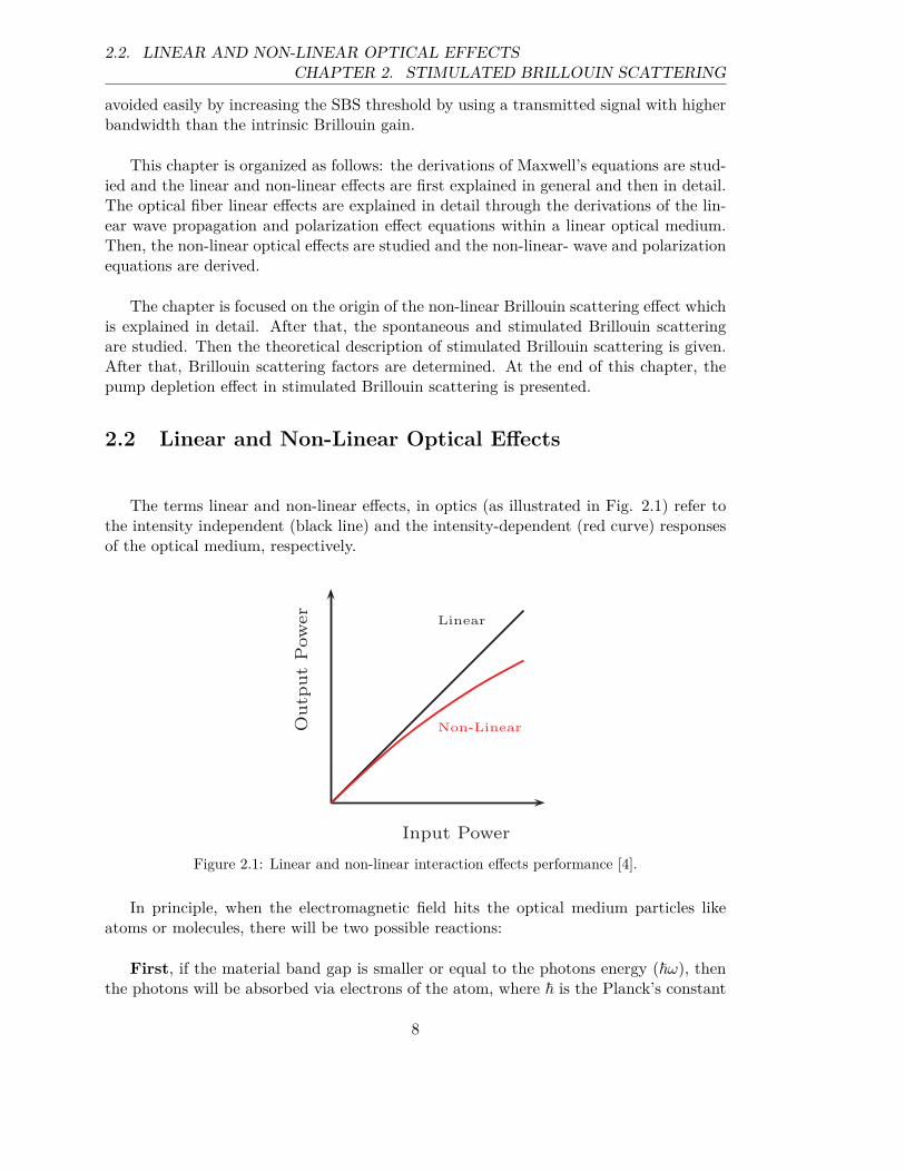
The terms linear and non-linear effects, in optics (as illustrated in Fig. 2.1) refer tothe intensity independent (black line) and the intensity-dependent (red curve) responsesof the optical medium, respectively.
Input Power
Outp
utPower
Linear
Non-Linear
Figure 2.1: Linear and non-linear interaction effects performance [4].
In principle, when the electromagnetic field hits the optical medium particles likeatoms or molecules, there will be two possible reactions:
First, if the material band gap is smaller or equal to the photons energy (~ω), thenthe photons will be absorbed via electrons of the atom, where ~ is the Planck’s constant
8
CHAPTER 2. STIMULATED BRILLOUIN SCATTERING2.2. LINEAR AND NON-LINEAR OPTICAL EFFECTS
and ω is the photon angular frequency. Therefore, the absorbed energy will be trans-formed into internal energy of the absorber, like thermal energy [29]. The reduction inthe intensity of the light wave propagating through a medium by absorption of a partof its photons is called attenuation. Normally, the absorption of waves is intensity in-dependent i.e. it is linear. Nevertheless, in optics the medium changes its transparencydepending on the intensity of the incident waves, and hence a saturable absorption i.e.non-linear absorption takes place. On the other hand, after the absorption the excitationdecay of the atom could take different forms with different energy and frequency from theoriginal wave. The most important and dominant in optical telecommunications is thespontaneous emission [7], since within some materials it can be transferred to the regionof stimulated emission by which lasers and Erbium-doped amplifiers (EDFA) based on.
Second, if the band gap of the material is larger than the photon energy, then andcontrary to the first case, no excitation towards the higher atom energy level will occur.However, the absorbed photon will upset the distribution of the charges within the atom.Since, the charges depend on the incident electric field, they will be accelerated. Addi-tionally, the emitted photons have the same energy and frequency of the original wave.Nevertheless, they have a different phase by which the linear optical effects originatefrom, such as diffraction, reflection, refraction, absorption and scattering. On the otherhand, in mediums like optical fibers which are made from silica glass, only the excitationin the way of charge acceleration can occur because they have a much higher band gapthan the photon energy.
To describe the linear effects in optical fibers, one should start from the Maxwell’sequations in vacuum that describe the interaction between the electromagnetic field (op-tical wave) and the material (optical fiber).
The Maxwell equations can be written as [30]:
∇ × E = −∂B
∂t(2.1a)
∇ × H = j +∂D
∂t(2.1b)
∇ · D = ρ (2.1c)
∇ · B = 0 (2.1d)
where ∇ is the Nabla operator, E and H are the electric and magnetic field vectors withthe corresponding flux densities (inductions) D and B, respectively. j is the current den-
sity and ρ is the carrier density. In Eq. 2.1a a time varying field (−∂B
∂t) is the origin of the
electric field eddies (∇×E). While, in Eq. 2.1b either the current density (j) or the time
dependent variation in the electric flux density (∂D
∂t) is the origin of magnetic eddies.
On the other hand, the existance of the sources (ρ) is the origin of the electric field as il-lustrated in Eq. 2.1c. Whereas, the magnetic field is free of sources as shown in Eq. 2.1d.
9

2.2. LINEAR AND NON-LINEAR OPTICAL EFFECTSCHAPTER 2. STIMULATED BRILLOUIN SCATTERING
In vacuum, the electric flux density (D) is related to the electric field vector (E) bythe vacuum permittivity (ε0), i.e. (D = ε0E) and within identity, (B = µ0H ), where(µ0) is the permeability [31, 32]. Since in vacuum there are no current (j) and carrier(ρ) densities, and by using the magnetic flux (B) instead of (H ) and (E) instead of (D)in Eq. 2.1b then Eq. 2.1 can be rewritten as follows:
∇ × E = −∂B
∂t(2.2a)
∇ × B = µ0ε0∂E
∂t(2.2b)
by substituting Eq. 2.2b into Eq. 2.2a, one can get a hyperbolic partial differentialequation which is the wave equation of the electromagnetic field that propagates invacuum and can be written as:
(c2∇2 − ∂2
∂t2
)E = 0 (2.3)
where c = 1/√ε0µ0 is the speed of light in vacuum (299,792,458 m/s) which is identical
for all waves in vacuum and (∇2) is the spatial Laplace operator (∆). Therefore, Eq. 2.3can be rewritten as follows:
∆E =1
c2
∂2E
∂t2(2.4)
The medium can be classified to:
1. Simple Medium.
2. Dispersive Medium.
3. Non-linear Medium.
4. Anisotropic Medium.
5. Bi-isotropic and Bi-anisotropic Medium.
Here, it will be discussed only the simple and non-linear dispersive medium.
2.2.1 Linear Effects
When a wave travels within a certain medium, that medium affects the propagatingwave and hence the wave equation itself. For example, the phenomena of conduction,polarization, and magnetization would take place. In principle, within vacuum (P=
10
CHAPTER 2. STIMULATED BRILLOUIN SCATTERING2.2. LINEAR AND NON-LINEAR OPTICAL EFFECTS
0), where (P) is the (polarization vector) which is the vector sum of the electric dipolemoments per unit volume, i.e. the volume density of electric dipole moment. For example,when an electric field of a condenser is applied to an insulator which placed into thatcondenser, then the charges of the insulator atoms will shift as an influence of the electricfield force. This phenomenon is called polarization [7]. Therefore, the electric flux densitywill be:
D = εrε0E (2.5)
where εr is the relative permittivity which depends on the medium, polarization and thefrequency of the incident wave.
The simple medium is the non-dispersive, linear and isotropic medium. Hence, withinsuch medium the vector (P) is parallel and linearly related to the external low strengthelectric field (E). In principle, the relation between them can be written as:
P = PL = ε0χE (2.6)
where PL refers to the linear polarization and (χ = εr − 1) is the electric susceptibilityand refers to the polarizability of the medium. Therefore, Eq. 2.5 can be rewritten byusing Eq. 2.6 as follows:
D = ε0 (1 + χ) E = ε0E + P (2.7)
The main difference between linear and non-linear optics is that the polarization is lin-early and non-linearly proportional to the electric field strength, respectively, i.e. de-pending on the strength of the applied electric field itself. For instance, by applying anoncoherent source like a light emitting diode, lamps or a sunlight, linear optical effectstake place. Substituting Eq. 2.7 in Eq. 2.1b and by assuming the current density (j=0)within the simple medium, one can get:
∇ × B = ε0µ0∂E
∂t+ µ0
∂P
∂t(2.8)
Thus, the wave equation for the stable, uniform simple medium will be:
∆E =1
c2
∂2E
∂t2+
1
ε0c2
∂2P
∂t2(2.9)
11
2.2. LINEAR AND NON-LINEAR OPTICAL EFFECTSCHAPTER 2. STIMULATED BRILLOUIN SCATTERING
The first term refers to the primary wave, while the second term refers to the secondarywave which originates from the polarization effect of the medium as a result of the externalwave. Both waves have the same frequency but with a relative phase shift. SubstitutingEq. 2.6 into Eq. 2.9 and by using Eq. 2.5, then the wave equation in a simple mediumwill be:
∆E =εr
c2
∂2E
∂t2(2.10)
In isotropic simple media, both the electric and polarization vectors are in the samedirection and the susceptibilities in all directions are equal. Additionally, in isotropicmedia the relative permittivity is a constant scalar [31]. On the other hand, in other (non-simple) media the relative permittivity is a complex second order tensor. The solution ofEq. 2.10 will be used to describe the linear optical effects. The main difference betweenthe wave propagation in vacuum and material is that: within material the wave willtravel slower than within vacuum by a factor of (1/n), where n is the real part of thecomplex refractive index (n(ω)) of the material and can be written as [7]:
n(ω) = n(ω) + jκ(ω) =√εr(ω) (2.11)
where (κ) and (ω) are the extinction coefficient and the molecule resonance frequencyof the material, respectively. In principle and referring to Eq. 2.9, the phase differencebetween the primary and secondary waves results in a wave propagation velocity differ-ence between vacuum and material. Therefore, the wave propagation velocity in materialdepends on the electromagnetic wave frequency and the material properties while this isnot the case within vacuum and the wave propagates with the velocity of light.
By assuming a plane transverse monochromatic wave which depends only on onecoordinate (z direction for example), then Eq. 2.10 will be:
∂2E
∂z2=
n2
c2
∂2E
∂t2(2.12)
here E = (Ex, Ey, 0) is perpendicular to the propagation direction z. The solution forEq. 2.12 will be:
E(z, t) =1
2(Eej(nk0z−ωt) + c.c)ei =
∣∣∣E∣∣∣ cos(nk0z − ωt+ ϕ0)ei (2.13)
where (E = Re(E) + j Im(E) = a + jb) is the complex amplitude of the wave, (ω = 2πf)
12
CHAPTER 2. STIMULATED BRILLOUIN SCATTERING2.2. LINEAR AND NON-LINEAR OPTICAL EFFECTS
is the angular frequency, (k0 = 2π/λ) is the wave number, ei is the unit vector for an
arbitrary i-direction and (ϕ0 = arctana
b) is the phase for z=0, therefore E can be written
as:
E = E0ejϕ0 (2.14)
In principle, all linear optical phenomena like: scattering, reflection, refraction, ab-sorption and diffraction can be described by Eq. 2.10 and for a particular condition(propagation in z direction) Eq. 2.13 can be used as a solution for Eq. 2.10. When Eq.2.11 is used in Eq. 2.13, then the wave propagation within insulator can be written as:
E(z, t) =1
2(Eej((n+jκ)k0z−ωt) + c.c)ei =
1
2(Ee−κk0zej(nk0z−ωt) + c.c)ei (2.15)
To understand the optical signal attenuation within optical fibers, a brief focus onEq. 2.15 will be given. Mainly, scattering and absorption are the origin of an attenuationin optical fibers. The term (Ee−κk0z) for instance, refers to the wave amplitude decreasewithin z distance propagation. Additionally, the wave intensity is related to the squareof the wave amplitude as:
I =1
2nε0c
∣∣∣E∣∣∣2
(2.16)
therefore, the wave intensity as a function of distance z can be written as:
I(z) = I0e−2k0κz = I0e
−αz (2.17)
where α denotes the attenuation constant (α = 2κk0 = 4πλ0κ) measured in km−1. For
example, α for a normal window glass is 11500 km−1, while it is 0.04 – 0.07 km−1 inoptical fibers for telecommunication wavelengths (1550 nm) [7]. Although the attenuationconstant is small for optical fibers compared to the ordinary glass and the power lossesare very low, they are not negligible if too long optical fibers are used. In principle, thewave intensity can be written as:
I =P
Aeff(2.18)
where P is the wave power and Aeff is the effective area of the fiber core that the
13
2.2. LINEAR AND NON-LINEAR OPTICAL EFFECTSCHAPTER 2. STIMULATED BRILLOUIN SCATTERING
wave propagates through. In case, when the effective area is constant during the wavepropagation, then both the intensity and the power of the wave are related to the squaredamplitude. Therefore, and referring to Eq. 2.17, the wave power will be introduced as:
dP (z)
dz= −αP (z) (2.19)
If z is changed with L: the propagation length, then Eq. 2.19 can be written as:
P (L) = P (0)e−αL (2.20)
where P (0) denotes the wave power at the fiber input.
2.2.2 Non-Linear Effects
Within a non-linear medium the relation between the polarization and the electricfield is non-linear . The non-linearity originates mainly from either microscopic or macro-scopic considerations. In general, the polarization density P can be considered as a prod-uct of dipole moment p induced by the applied electric field E and the dipole momentsnumber density N , i.e. P = pN [33]. Within the microscopic consideration, when theelectric field strength is high enough typically 105-108 V/m, i.e. it has values near theinter-atomic electric field, then the relation between the dipole moment p and the elec-tric field E becomes non-linear. In principle, the dipole moment p = −ex, here x isthe mass displacement which has a charge −e related to the applied electric force −eE.When Hooke’s law is satisfied [34], i.e. the restraining force is linearly proportional tothe displacement then the equilibrium displacement x is proportional to E. Hence, P islinearly related to E and the medium is linear. Additionally, when the restraining force isnon-linearly functioning with the displacement, then the equilibrium displacement x andthe polarization density P both are non-linearly related to the electric field E. Therefore,the medium can be considered as non-linear.
In principle, if the dipole moments number density N of the medium depends on theincident electric field E, then the macroscopic consideration takes place. In this case, thepolarization is the summation of the discrete macroscopic field induced dipole momentsof ith molecule, depending on the macroscopic symmetry of the medium. Hence, thepolarization can be expressed as:
P(t) =N∑
i=1
Pi(t) (2.21)
14
CHAPTER 2. STIMULATED BRILLOUIN SCATTERING2.2. LINEAR AND NON-LINEAR OPTICAL EFFECTS
and therefore the macroscopic polarization can be expressed as a power Taylor series[33, 35]:
P(t) = ε0(χ(1)E(t) + χ(2)E2(t) + χ(3)E3(t) + ...) (2.22)
The susceptibility terms χ(i=1,2,3,...) (linear and non-linear) are tensors of rank (i+1).In principle, the susceptibility defines the relation between the induced polarization if itis linear or non-linear. Additionally, it describes whether the electric fields produce phaseshifts or waves with new frequencies, and if the incident field will be absorbed or ampli-fied. The first order susceptibility χ(1) refers to the dipole excitation with bound and freeelectrons produced by a single photon. In principle, the real part of χ(1) is related to thereal part of the refractive index, while the imaginary part of χ(1) refers to the gain or loss.
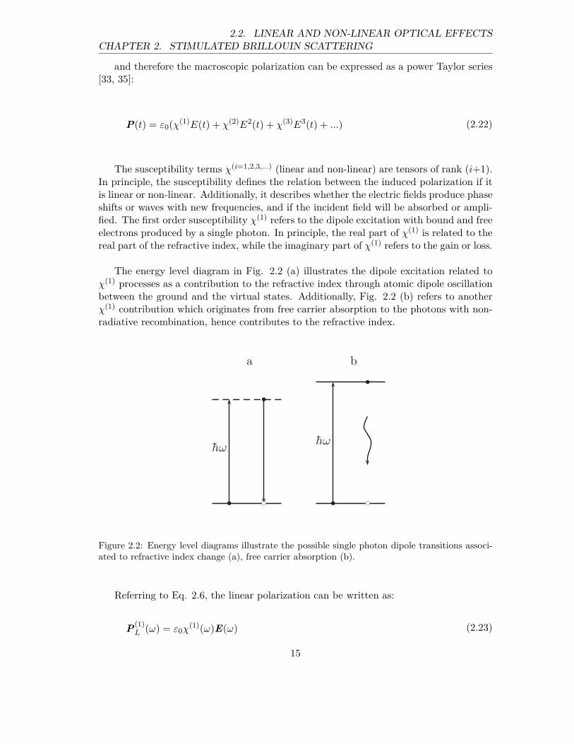
The energy level diagram in Fig. 2.2 (a) illustrates the dipole excitation related toχ(1) processes as a contribution to the refractive index through atomic dipole oscillationbetween the ground and the virtual states. Additionally, Fig. 2.2 (b) refers to anotherχ(1) contribution which originates from free carrier absorption to the photons with non-radiative recombination, hence contributes to the refractive index.
hω
!
a
hω
!
b
Figure 2.2: Energy level diagrams illustrate the possible single photon dipole transitions associ-ated to refractive index change (a), free carrier absorption (b).
Referring to Eq. 2.6, the linear polarization can be written as:
P(1)L (ω) = ε0χ
(1)(ω)E(ω) (2.23)
15
2.2. LINEAR AND NON-LINEAR OPTICAL EFFECTSCHAPTER 2. STIMULATED BRILLOUIN SCATTERING
Within the same frequency ω, both the polarization and the incident electric field arelinearly related including the linearity constant χ(1). Hence and referring to Eq. 2.9, theprimary wave promotes the dipoles to oscillate with its frequency ω and the secondarywave has a phase shift without any new frequency components. Having the fact that thesusceptibility is a tensor of (i+1) rank, then Eq. 2.23 can be written as:
P(1)Li (ω) = ε0
∑
j
χ(1)ij (ω)Ej(ω) (2.24)
where i, j = x, y, z. Here, the first order susceptibility tensor (χ(1)ij ) contains nine elements
(31x3). Depending on the material symmetry arguments, the susceptibility tensor canbe reduced. For example and according to [36], the first order susceptibility tensor χ(1)
of an isotropic material contains a single frequency dependent element. As mentionedearlier, this contributes to refractive index.
The second order susceptibility χ(2) depends on the combination of the input frequen-cies, since the external fields can interact with each other and nine field combinations arepossible. For example, when the incident field has two different frequencies, then theyachieve a second order polarization at the sum, difference or multiples of the incidentfrequencies. And therefore, the secondary wave contains new as well as the original fre-quency components. Additionally, the second order susceptibility χ(2) is related to theincident field vectors as well as the field vector of the polarization. Therefore, the secondorder non-linear polarization which connect two incident fields can be written as:
P(2)NLi(ω1, ω2) = ε0χ
(2)(ω1, ω2)E(ω1)E(ω2) (2.25)
Having the fact that the second order susceptibility χ(2)ijk has 27 elements (32x3) and only
9 field combinations (32) are possible, therefore Eq. 2.25 can be written as:
P(2)NLi(ω1, ω2) = ε0
∑
jk
χ(2)ijk(ω1, ω2)Ej(ω1)Ek(ω2) (2.26)
where, i, j, k = x, y, z.Eq. 2.25 is responsible for all the second order non-linear effects. Since optical fibers
are made from silica glass which has a symmetry center, all the 27 tensor elements of thesecond order susceptibility χ(2) are zero. Therefore, the second order non-linear effectscan be ignored.
The third order susceptibility tensor χ(3) consists of 81 elements (33×3) for threedirections and the third order polarization P 3
NL connects three fields, therefore 27 fieldcombinations (33) are possible. As in the second order case, the polarization will beproduced at the sum, difference or multiples of the incident frequencies. The third orderpolarization can be written as:
P(3)NLi(ω1, ω2, ω3) = ε0χ
(3)(ω1, ω2, ω3)E(ω1)E(ω2)E(ω3) (2.27)
16
CHAPTER 2. STIMULATED BRILLOUIN SCATTERING2.3. BRILLOUIN SCATTERING PHYSICS
and in summation form:
P(3)NLi(ω1, ω2, ω3) = ε0
∑
jkl
χ(3)ijkl(ω1, ω2, ω3)Ej(ω1)Ek(ω2)E l(ω3) (2.28)
where, i, j, k, l = x, y, z directions.
Referring to Eq. 2.11 where n =√εr =
√χ(1) + 1, the non-linear wave equation for
a non-linear medium will be:
∆E =1
c2
∂2E
∂t2︸ ︷︷ ︸L
+1
c2χ(1)∂
2E
∂t2+
1
c2χ(2)∂
2EE
∂t2+
1
c2χ(3)∂
2EEE
∂t2+ ...
︸ ︷︷ ︸NL
(2.29)
and therefore:
∆E − n2
c2
∂2E
∂t2=
1
c2
∂2
∂t2
(χ(2)EE + χ(3)EEE + ...
)(2.30)
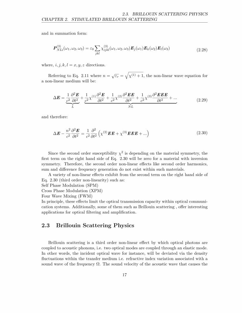
Since the second order susceptibility χ2 is depending on the material symmetry, thefirst term on the right hand side of Eq. 2.30 will be zero for a material with inversionsymmetry. Therefore, the second order non-linear effects like second order harmonics,sum and difference frequency generation do not exist within such materials.
A variety of non-linear effects exhibit from the second term on the right hand side ofEq. 2.30 (third order non-linearity) such as:Self Phase Modulation (SPM)Cross Phase Modulation (XPM)Four Wave Mixing (FWM)In principle, these effects limit the optical transmission capacity within optical communi-cation systems. Additionally, some of them such as Brillouin scattering , offer interestingapplications for optical filtering and amplification.
2.3 Brillouin Scattering Physics
Brillouin scattering is a third order non-linear effect by which optical photons arecoupled to acoustic phonons, i.e. two optical modes are coupled through an elastic mode.In other words, the incident optical wave for instance, will be deviated via the densityfluctuations within the transfer medium i.e. refractive index variation associated with asound wave of the frequency Ω. The sound velocity of the acoustic wave that causes the
17

2.3. BRILLOUIN SCATTERING PHYSICSCHAPTER 2. STIMULATED BRILLOUIN SCATTERING
density fluctuations (grating) is denoted as (νA). The frequencies of incident (pump),Stokes (scattered) and acoustic waves are denoted as fP , fS and fA, respectively. Thewave vectors of the pump, Stokes and acoustic waves will be denoted as: kP ,kS and kA,respectively.
Fig. 2.3 illustrates the Brillouin scattering process via medium induced density vari-ations which originate from the acoustic wave in two directions, (a) and (b), travelingwith sound velocity (νA) and having the angle θ with the incident optical pump field.
(a)
νA
kS
θ
kP kS
kP
kA
(b)
νA
kS
θ
kP kS
kP
kA
Figure 2.3: Brillouin scattering process illustration at medium density fluctuations for two direc-tions (a) and (b) with sound velocity (νA) and wave vectors representation.
The Energy (~ω) and momentum (~k) are conserved during the scattering process.Therefore, according to the vector diagrams in Fig. 2.3 the condition can be written as:
kS = kP ∓ kA (2.31)
and hence, the scattered wave frequency will be:
fS = fP ∓ fA (2.32)
18
CHAPTER 2. STIMULATED BRILLOUIN SCATTERING2.3. BRILLOUIN SCATTERING PHYSICS
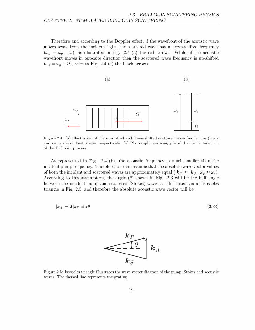
Therefore and according to the Doppler effect, if the wavefront of the acoustic wavemoves away from the incident light, the scattered wave has a down-shifted frequency(ωs = ωp − Ω), as illustrated in Fig. 2.4 (a) the red arrows. While, if the acousticwavefront moves in opposite direction then the scattered wave frequency is up-shifted(ωs = ωp + Ω), refer to Fig. 2.4 (a) the black arrows.
(a)
Ωωp
ωs
(b)
ωp ωs
Ω
Figure 2.4: (a) Illustration of the up-shifted and down-shifted scattered wave frequencies (blackand red arrows) illustrations, respectively. (b) Photon-phonon energy level diagram interactionof the Brillouin process.
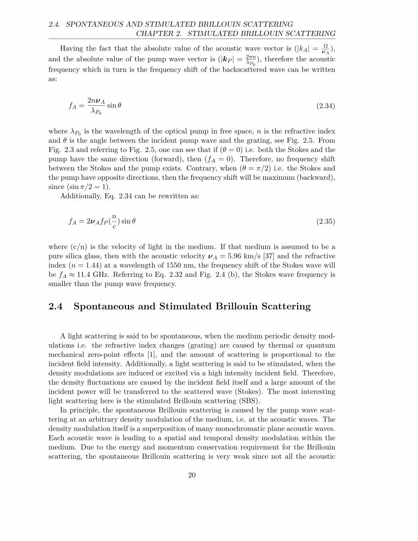
As represented in Fig. 2.4 (b), the acoustic frequency is much smaller than theincident pump frequency. Therefore, one can assume that the absolute wave vector valuesof both the incident and scattered waves are approximately equal (|kP | ≈ |kS | , ωp ≈ ωs).According to this assumption, the angle (θ) shown in Fig. 2.3 will be the half anglebetween the incident pump and scattered (Stokes) waves as illustrated via an isoscelestriangle in Fig. 2.5, and therefore the absolute acoustic wave vector will be:
|kA| = 2 |kP | sin θ (2.33)
kP
kS
kAθ
Figure 2.5: Isosceles triangle illustrates the wave vector diagram of the pump, Stokes and acousticwaves. The dashed line represents the grating.
19
2.4. SPONTANEOUS AND STIMULATED BRILLOUIN SCATTERINGCHAPTER 2. STIMULATED BRILLOUIN SCATTERING
Having the fact that the absolute value of the acoustic wave vector is (|kA| = ΩνA
),
and the absolute value of the pump wave vector is (|kP | = 2πnλP0
), therefore the acoustic
frequency which in turn is the frequency shift of the backscattered wave can be writtenas:
fA =2nνA
λP0
sin θ (2.34)
where λP0 is the wavelength of the optical pump in free space, n is the refractive indexand θ is the angle between the incident pump wave and the grating, see Fig. 2.5. FromFig. 2.3 and referring to Fig. 2.5, one can see that if (θ = 0) i.e. both the Stokes and thepump have the same direction (forward), then (fA = 0). Therefore, no frequency shiftbetween the Stokes and the pump exists. Contrary, when (θ = π/2) i.e. the Stokes andthe pump have opposite directions, then the frequency shift will be maximum (backward),since (sin π/2 = 1).
Additionally, Eq. 2.34 can be rewritten as:
fA = 2νAfP (n
c) sin θ (2.35)
where (c/n) is the velocity of light in the medium. If that medium is assumed to be apure silica glass, then with the acoustic velocity νA = 5.96 km/s [37] and the refractiveindex (n = 1.44) at a wavelength of 1550 nm, the frequency shift of the Stokes wave willbe fA ≈ 11.4 GHz. Referring to Eq. 2.32 and Fig. 2.4 (b), the Stokes wave frequency issmaller than the pump wave frequency.
2.4 Spontaneous and Stimulated Brillouin Scattering
A light scattering is said to be spontaneous, when the medium periodic density mod-ulations i.e. the refractive index changes (grating) are caused by thermal or quantummechanical zero-point effects [1], and the amount of scattering is proportional to theincident field intensity. Additionally, a light scattering is said to be stimulated, when thedensity modulations are induced or excited via a high intensity incident field. Therefore,the density fluctuations are caused by the incident field itself and a large amount of theincident power will be transferred to the scattered wave (Stokes). The most interestinglight scattering here is the stimulated Brillouin scattering (SBS).
In principle, the spontaneous Brillouin scattering is caused by the pump wave scat-tering at an arbitrary density modulation of the medium, i.e. at the acoustic waves. Thedensity modulation itself is a superposition of many monochromatic plane acoustic waves.Each acoustic wave is leading to a spatial and temporal density modulation within themedium. Due to the energy and momentum conservation requirement for the Brillouinscattering, the spontaneous Brillouin scattering is very weak since not all the acoustic
20

CHAPTER 2. STIMULATED BRILLOUIN SCATTERING2.4. SPONTANEOUS AND STIMULATED BRILLOUIN SCATTERING
waves could generate a Stokes wave.
Contrary to the spontaneous Brillouin scattering, the SBS is a result of a high inci-dent field in the optical medium. Therefore, a beating (interference) between the incidentpump wave and the back scattered wave (Stokes) will take place. In principle when thepump power is high enough, then the power transfer from the pump to the Stokes ishigher than the attenuation within the medium. Additionally, the interference betweenthe pump and Stokes waves contains a frequency component at a frequency differencebetween the pump and Stokes waves i.e. at the acoustic frequency (Ω) and in the direc-tion of the pump wave.
The medium will response to that interference in a way that will act as a new sourcefor the sound wave and increase the acoustic amplitude. Hence, the interference re-sults into reinforce (amplification) to the acoustic wave. In principle, the superpositionbetween the pump and Stokes waves results in a fading with the acoustic frequency.Therefore, an intensity modulation in the direction of the pump wave will take place.Afterwords, the intensity modulation will be translated to a density modulation throughan electrostriction effect. A high pump wave results in a higher interference and there-fore, a stronger acoustic wave and stronger Stokes will be generated and so on, which iscalled stimulation. Under certain conditions i.e. sufficient temporal and spatial coher-ence of the pump source, the positive interference feedback achieves exponential growth(amplification) of the Stokes amplitude [38, 39]:
IS(Output)= IS(Input)
exp(gBIP (L)Leff )︸ ︷︷ ︸
G
(2.36)
Leff =[1 − exp (−αz)]
α(2.37)
where IS(Output)and IS(Input)
are the scattered wave (Stokes) output and input intensitiesat z = 0 and z = L, respectively as illustrated in Fig. 2.6.
The length of the optical fiber is denoted as L and the specific length position as z.The factor G refers to the Stokes amplification as a function of the gain coefficient gB,pump intensity IP (L) and the fiber interaction length (effective length ) Leff , see Fig. 2.7.The gain coefficient gB is a function of the frequency shift ∆Ω from the gain center anddepends on the optical fiber properties and the scattering environments. Eq. 2.36 (whichwill be derived in the next section) shows that the Stokes intensity strongly dependson the pump intensity IP (L), therefore if the pump intensity is increased by a smallmagnitude, the Stokes intensity will be increased by orders of magnitude. Additionally,at the gain center when the frequency shift ∆Ω = 0 which is called resonance frequencyand will be denoted as ΩB(0), the Stokes intensity reaches the maximum value which iscalled gain maximum or resonance condition (gB(0)).
21
2.4. SPONTANEOUS AND STIMULATED BRILLOUIN SCATTERINGCHAPTER 2. STIMULATED BRILLOUIN SCATTERING
I P I S
L
d
z = Lz = 0
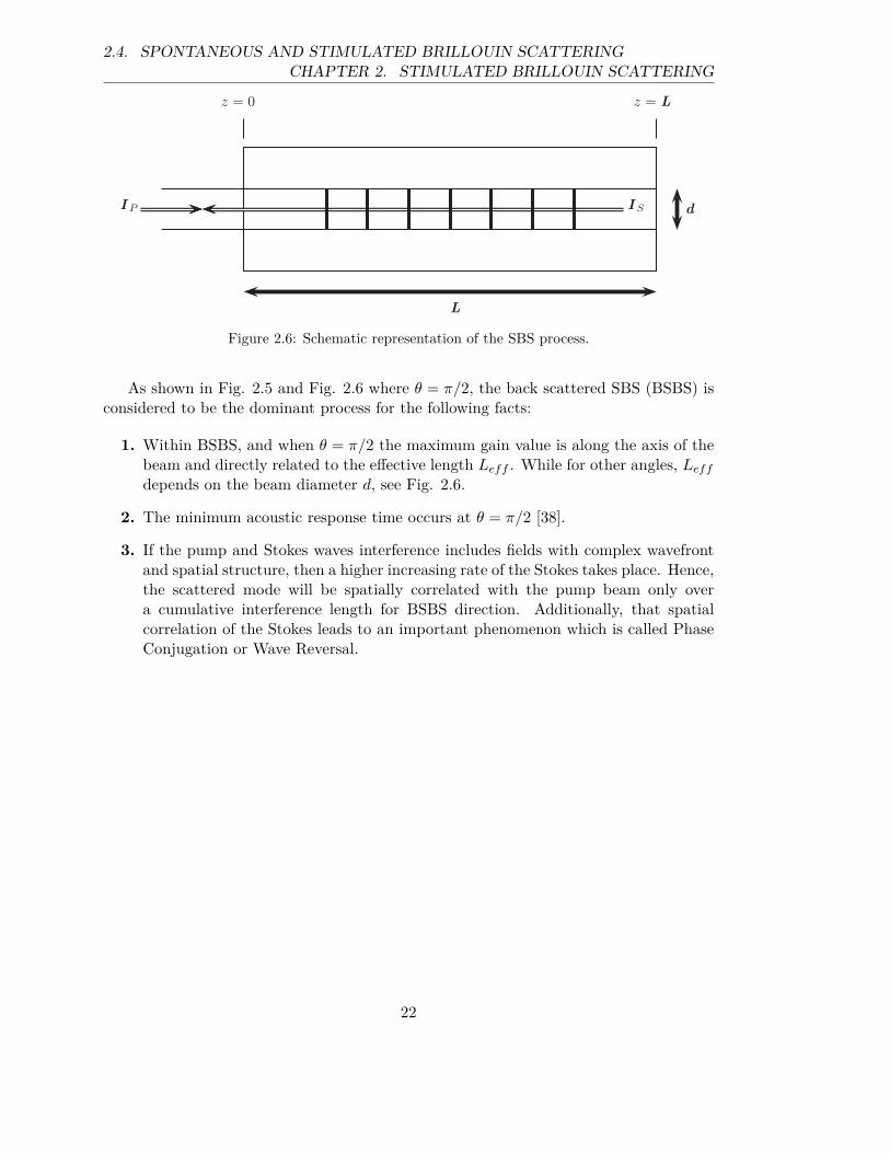
Figure 2.6: Schematic representation of the SBS process.
As shown in Fig. 2.5 and Fig. 2.6 where θ = π/2, the back scattered SBS (BSBS) isconsidered to be the dominant process for the following facts:
1. Within BSBS, and when θ = π/2 the maximum gain value is along the axis of thebeam and directly related to the effective length Leff . While for other angles, Leff
depends on the beam diameter d, see Fig. 2.6.
2. The minimum acoustic response time occurs at θ = π/2 [38].
3. If the pump and Stokes waves interference includes fields with complex wavefrontand spatial structure, then a higher increasing rate of the Stokes takes place. Hence,the scattered mode will be spatially correlated with the pump beam only overa cumulative interference length for BSBS direction. Additionally, that spatialcorrelation of the Stokes leads to an important phenomenon which is called PhaseConjugation or Wave Reversal.
22
CHAPTER 2. STIMULATED BRILLOUIN SCATTERING2.5. MATHEMATICAL DESCRIPTION OF SBS
0 10 20 30 40 50 60 700
3
6
9
12
15
18
21
Effe
ctiv
e Le
ngth
[km
]
Optical Fiber Length [km]
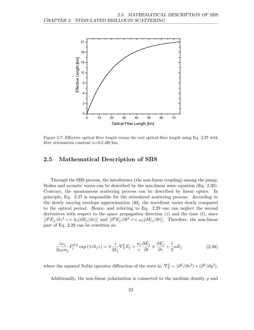
Figure 2.7: Effective optical fiber length versus the real optical fiber length using Eq. 2.37 withfiber attenuation constant α=0.2 dB/km.
2.5 Mathematical Description of SBS
Through the SBS process, the interference (the non-linear coupling) among the pump,Stokes and acoustic waves can be described by the non-linear wave equation (Eq. 2.30).Contrary, the spontaneous scattering process can be described by linear optics. Inprinciple, Eq. 2.27 is responsible for the stimulated scattering process. According tothe slowly varying envelope approximation [40], the wavefront varies slowly comparedto the optical period. Hence, and referring to Eq. 2.29 one can neglect the secondderivatives with respect to the space propagation direction (z) and the time (t), since[∂2Ej/∂z
2 << kj(∂Ej/∂z)]
and[∂2Ej/∂t
2 << ωj(∂Ej/∂t)]. Therefore, the non-linear
part of Eq. 2.29 can be rewritten as:
iωj
2ǫ0cnjPNL
j exp (∓ikjz) = ∓ i
2kj∇2
TEj +nj
c
∂Ej
∂t∓ ∂Ej
∂z+
1
2αEj (2.38)
where the squared Nabla operator diffraction of the wave is: ∇2T = (∂2/∂x2) + (∂2/∂y2).
Additionally, the non-linear polarization is connected to the medium density ρ and
23
2.5. MATHEMATICAL DESCRIPTION OF SBSCHAPTER 2. STIMULATED BRILLOUIN SCATTERING
the temperature T as follows [38]:
PNL =
(∂ε
∂ρ
)
T
∆ρ
︸ ︷︷ ︸Electrostriction
+
(∂ε
∂T
)
ρ∆T
︸ ︷︷ ︸Absorption
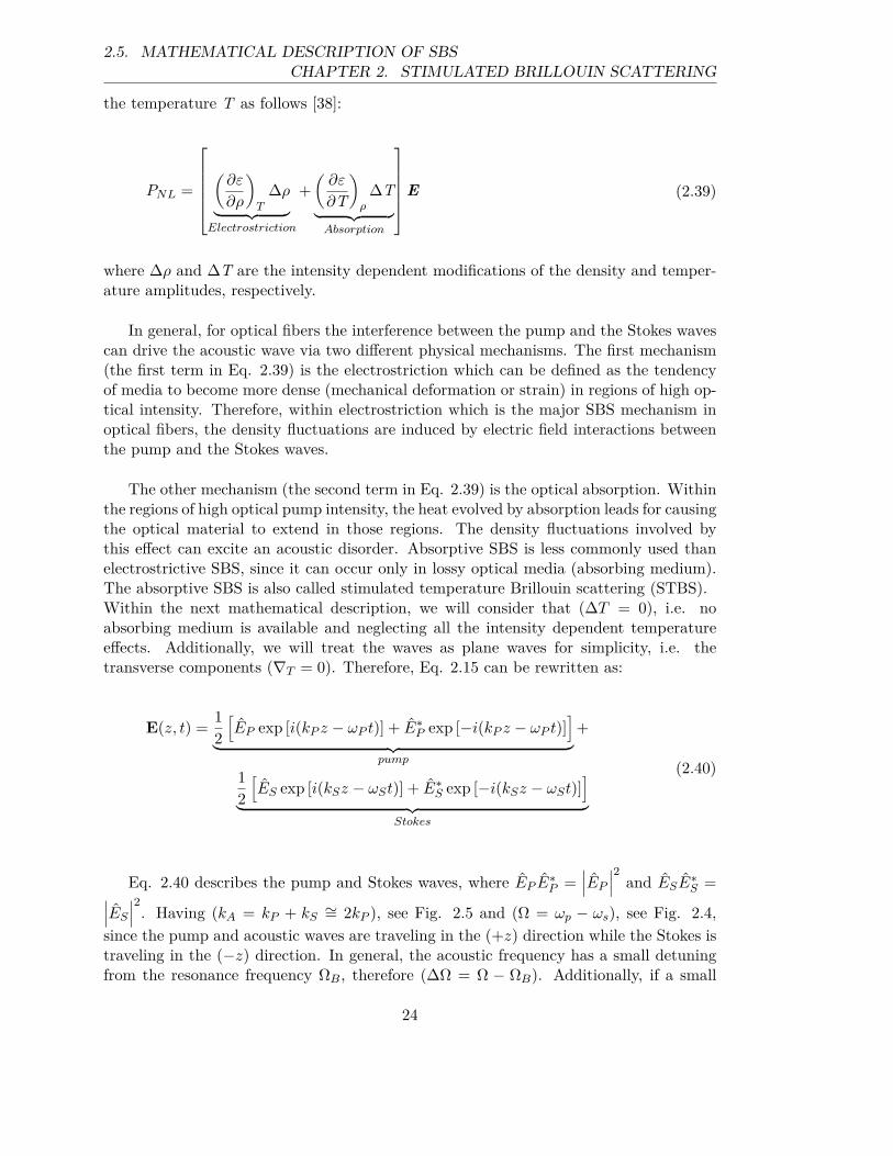
E (2.39)
where ∆ρ and ∆T are the intensity dependent modifications of the density and temper-ature amplitudes, respectively.
In general, for optical fibers the interference between the pump and the Stokes wavescan drive the acoustic wave via two different physical mechanisms. The first mechanism(the first term in Eq. 2.39) is the electrostriction which can be defined as the tendencyof media to become more dense (mechanical deformation or strain) in regions of high op-tical intensity. Therefore, within electrostriction which is the major SBS mechanism inoptical fibers, the density fluctuations are induced by electric field interactions betweenthe pump and the Stokes waves.
The other mechanism (the second term in Eq. 2.39) is the optical absorption. Withinthe regions of high optical pump intensity, the heat evolved by absorption leads for causingthe optical material to extend in those regions. The density fluctuations involved bythis effect can excite an acoustic disorder. Absorptive SBS is less commonly used thanelectrostrictive SBS, since it can occur only in lossy optical media (absorbing medium).The absorptive SBS is also called stimulated temperature Brillouin scattering (STBS).Within the next mathematical description, we will consider that (∆T = 0), i.e. noabsorbing medium is available and neglecting all the intensity dependent temperatureeffects. Additionally, we will treat the waves as plane waves for simplicity, i.e. thetransverse components (∇T = 0). Therefore, Eq. 2.15 can be rewritten as:
E(z, t) =1
2
[EP exp [i(kP z − ωP t)] + E∗
P exp [−i(kP z − ωP t)]]
︸ ︷︷ ︸pump
+
1
2
[ES exp [i(kSz − ωSt)] + E∗
S exp [−i(kSz − ωSt)]]
︸ ︷︷ ︸Stokes
(2.40)
Eq. 2.40 describes the pump and Stokes waves, where EP E∗
P =∣∣∣EP
∣∣∣2
and ESE∗
S =∣∣∣ES
∣∣∣2. Having (kA = kP + kS
∼= 2kP ), see Fig. 2.5 and (Ω = ωp − ωs), see Fig. 2.4,
since the pump and acoustic waves are traveling in the (+z) direction while the Stokes istraveling in the (−z) direction. In general, the acoustic frequency has a small detuningfrom the resonance frequency ΩB, therefore (∆Ω = Ω − ΩB). Additionally, if a small
24
CHAPTER 2. STIMULATED BRILLOUIN SCATTERING2.5. MATHEMATICAL DESCRIPTION OF SBS
variation in the medium density is considered (∆ρ = ρ′ − ρ0): where ρ0 is the average
density, which is evolved by the pump field, the medium density wave can be written as:
∆ρ =1
2[ρ exp [i(kAz − ωt)] + c.c] (2.41)
As mentioned earlier, the medium becomes more dense in the regions of high opticalfield, since the medium is mainly response to the superposition of the pump and Stokeswaves, i.e. at the beat frequency (Ω = ωp − ωs) which travels at a velocity:
νA =ωp − ωs
kP + kS(2.42)
Therefore, and according to the energy and momentum conservation (correspondingto resonance), the electrostrictive deriving force remains in phase with the generatedacoustic wave. Hence, and from Eq. 2.28 the pump and Stokes field equations can bewritten as [38]:
∂EP
∂z+n
c
∂EP
∂t+
1
2αEP =
iωp
4cnp
γe
ρ0ESρ (2.43)
−∂ES
∂z+n
c
∂ES
∂t+
1
2αES =
iωs
4cns
γe
ρ0EPρ
∗ (2.44)
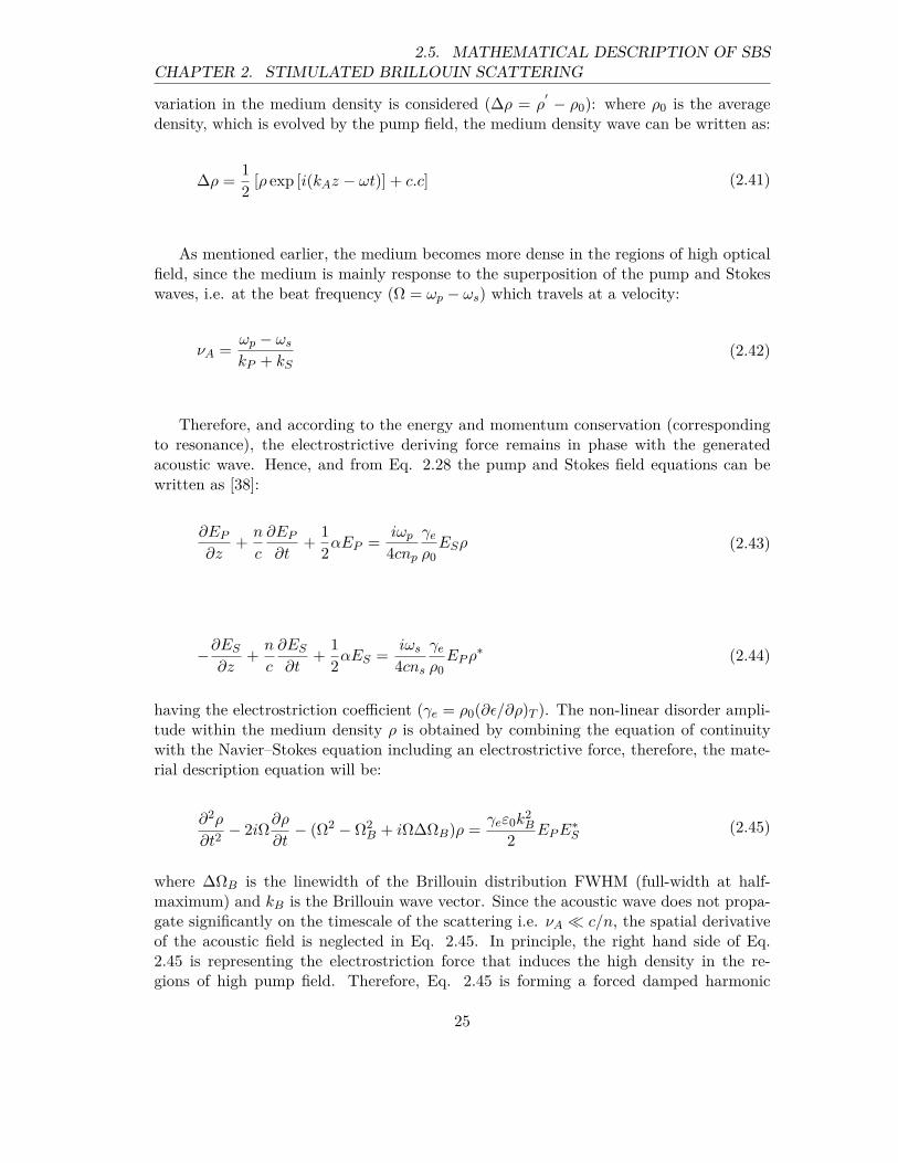
having the electrostriction coefficient (γe = ρ0(∂ǫ/∂ρ)T ). The non-linear disorder ampli-tude within the medium density ρ is obtained by combining the equation of continuitywith the Navier–Stokes equation including an electrostrictive force, therefore, the mate-rial description equation will be:
∂2ρ
∂t2− 2iΩ
∂ρ
∂t− (Ω2 − Ω2
B + iΩ∆ΩB)ρ =γeε0k
2B
2EPE
∗
S(2.45)
where ∆ΩB is the linewidth of the Brillouin distribution FWHM (full-width at half-maximum) and kB is the Brillouin wave vector. Since the acoustic wave does not propa-gate significantly on the timescale of the scattering i.e. νA ≪ c/n, the spatial derivativeof the acoustic field is neglected in Eq. 2.45. In principle, the right hand side of Eq.2.45 is representing the electrostriction force that induces the high density in the re-gions of high pump field. Therefore, Eq. 2.45 is forming a forced damped harmonic
25

2.5. MATHEMATICAL DESCRIPTION OF SBSCHAPTER 2. STIMULATED BRILLOUIN SCATTERING
oscillator. Additionally, in practical case one can assume that the acoustic wave ampli-tude growth is slow in comparison to the acoustic frequency, therefore the approximation(∂2ρ/∂t2 ≪ 2Ω(∂ρ/∂t)) is valid. In principle, if the SBS process is driven by a very shortpulse i.e. the acoustic period ≈ 1 ns, then the above approximation is not valid.
As mentioned earlier, if a small detuning from resonance is considered, i.e. (Ω2−Ω2B =
(Ω + ΩB)(Ω − ΩB) ≈ 2ΩB∆Ω), then the acoustic wave can be described as:
∂ρ
∂t+ (−i∆Ω +
∆ΩB
2)ρ =
iγeε0kB
4νAEPE
∗
S (2.46)
In general, and by the consideration of plane wave interaction, the SBS process canbe described by Equations 2.43, 2.44 and 2.46 regarding time and space. In case of asteady state set of equations, i.e. the time derivatives are zero, then the density wavewill be:
ρ =iγeε0kB
4νA
1
(1 − 2i∆Ω/∆ΩB)EPE
∗
S (2.47)
Having the intensity-field relation (Ij = ε0cn |Ej |2 /2) and by inserting Eq. 2.47 intoequations 2.43 and 2.44, one can obtain the set of the two coupled non-linear equa-tions that describes the relation between the pump and Stokes waves for approximatelymonochromatic waves or relatively long pulses:
dIP
dz= −gBpIP IS (2.48)
dIS
dz= −gBsIP IS (2.49)
As mentioned earlier, that the frequency shift between the pump and Stokes wave issmall (fA ≈ 11.4 GHz). This leads to the consideration that the Stokes wave frequency isapproximately equal to the pump wave frequency. Hence, one can assume that both theBrillouin gain coefficient and the attenuation factor are approximately equal for the pumpand Stokes waves. Therefore, (gBp ≈ gBs, αp ≈ αs). Now, the steady state Brillouin gaincoefficient (gB) can be given as:
gB = ΩB(0)1
1 + (2∆Ω/∆ΩB)2 (2.50)
26
CHAPTER 2. STIMULATED BRILLOUIN SCATTERING2.5. MATHEMATICAL DESCRIPTION OF SBS
and the maximum gain coefficient at resonance is:
ΩB(0) =ω2
s(γe)2
c3νAρ0∆ΩB(2.51)
Additionally, if the loss inside the medium is considered, then the attenuation factorα should be added. Therefore, Equations 2.48 and 2.49 can be rewritten as:
dIP
dz= −gBIP IS − αpIP (2.52)
dIS
dz= −gBIP IS + αsIS (2.53)
where (αp ≈ αs = α) are the attenuation constants for the pump and Stokes wave,respectively, which both are approximately equal, as mentioned earlier. In principle,equations 2.52 and 2.53 show that there is a power transfer from the pump wave to theStokes wave (−gB), in addition it is attenuated within the medium via (α). The Stokeswave growth in the backward direction (−z) and shows an exponential growth while thepump wave shows a depletion. With low intensities, the pump depletion is rather small.Therefore, the first term in Eq. 2.52 can be neglected and can be represented as:
IP (z) = IP (0) exp (−αz) (2.54)
Eq. 2.54, shows that, under the above simplifications the pump intensity dependsonly on the attenuation of the fiber, and at any fiber position (L) the pump intensitycan be written as:
IP (L) = IP (0)
∫ L
0e−αzdz =
IP (0)
α(1 − e−αL) = IP (0)Leff (2.55)
If the pump intensity is not effected by the Brillouin process, then Eq. 2.53 can berepresented as:
dIS
dz= (−gBIP + α)IS (2.56)
27
2.5. MATHEMATICAL DESCRIPTION OF SBSCHAPTER 2. STIMULATED BRILLOUIN SCATTERING
Now, by substituting Eq. 2.55 into Eq. 2.56, the Stokes intensity at any position (L) canbe given as:
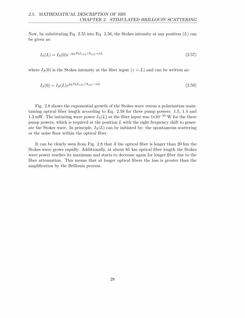
IS(L) = IS(0)e−gBP0Leff /Aeff +αL (2.57)
where IS(0) is the Stokes intensity at the fiber input (z = L) and can be written as:
IS(0) = IS(L)egBP0Leff /Aeff −αL (2.58)
Fig. 2.8 shows the exponential growth of the Stokes wave versus a polarization main-taining optical fiber length according to Eq. 2.58 for three pump powers: 1.5, 1.4 and1.3 mW. The initiating wave power IS(L) at the fiber input was 1x10⁻¹⁰ W for the threepump powers, which is required at the position L with the right frequency shift to gener-ate the Stokes wave. In principle, IS(L) can be initiated by: the spontaneous scatteringor the noise floor within the optical fiber.
It can be clearly seen from Fig. 2.8 that if the optical fiber is longer than 20 km theStokes wave grows rapidly. Additionally, at about 65 km optical fiber length the Stokeswave power reaches its maximum and starts to decrease again for longer fiber due to thefiber attenuation. This means that at longer optical fibers the loss is greater than theamplification by the Brillouin process.
28
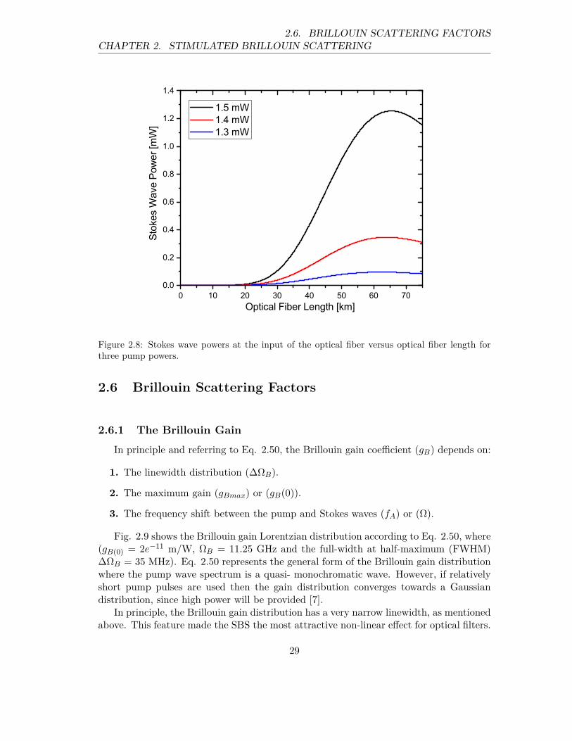
CHAPTER 2. STIMULATED BRILLOUIN SCATTERING2.6. BRILLOUIN SCATTERING FACTORS
0 10 20 30 40 50 60 700.0
0.2
0.4
0.6
0.8
1.0
1.2
1.4
Stok
es W
ave
Pow
er [m
W]
Optical Fiber Length [km]
1.5 mW 1.4 mW 1.3 mW
Figure 2.8: Stokes wave powers at the input of the optical fiber versus optical fiber length forthree pump powers.
2.6 Brillouin Scattering Factors
2.6.1 The Brillouin Gain
In principle and referring to Eq. 2.50, the Brillouin gain coefficient (gB) depends on:
1. The linewidth distribution (∆ΩB).
2. The maximum gain (gBmax) or (gB(0)).
3. The frequency shift between the pump and Stokes waves (fA) or (Ω).
Fig. 2.9 shows the Brillouin gain Lorentzian distribution according to Eq. 2.50, where(gB(0) = 2e−11 m/W, ΩB = 11.25 GHz and the full-width at half-maximum (FWHM)∆ΩB = 35 MHz). Eq. 2.50 represents the general form of the Brillouin gain distributionwhere the pump wave spectrum is a quasi- monochromatic wave. However, if relativelyshort pump pulses are used then the gain distribution converges towards a Gaussiandistribution, since high power will be provided [7].
In principle, the Brillouin gain distribution has a very narrow linewidth, as mentionedabove. This feature made the SBS the most attractive non-linear effect for optical filters.
29
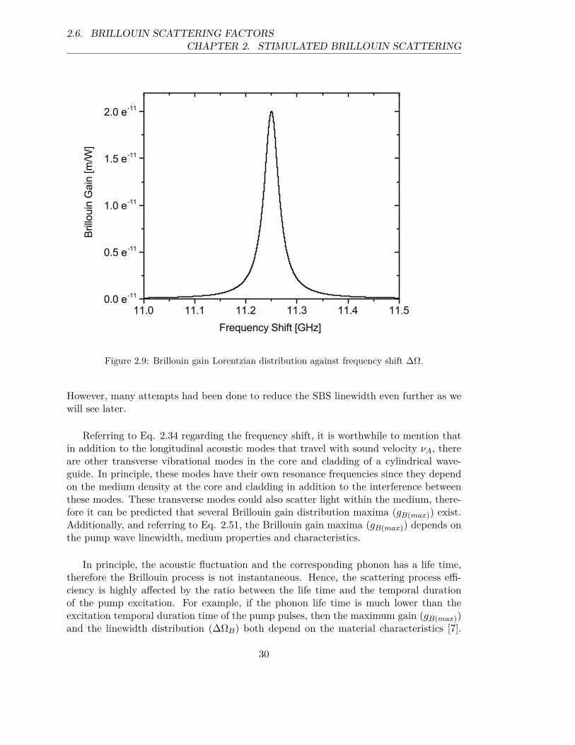
2.6. BRILLOUIN SCATTERING FACTORSCHAPTER 2. STIMULATED BRILLOUIN SCATTERING
11.0 11.1 11.2 11.3 11.4 11.50.0 e-11
0.5 e-11
1.0 e-11
1.5 e-11
2.0 e-11
Brillo
uin
Gai
n [m
/W]
Frequency Shift [GHz]
Figure 2.9: Brillouin gain Lorentzian distribution against frequency shift ∆Ω.
However, many attempts had been done to reduce the SBS linewidth even further as wewill see later.
Referring to Eq. 2.34 regarding the frequency shift, it is worthwhile to mention thatin addition to the longitudinal acoustic modes that travel with sound velocity νA, thereare other transverse vibrational modes in the core and cladding of a cylindrical wave-guide. In principle, these modes have their own resonance frequencies since they dependon the medium density at the core and cladding in addition to the interference betweenthese modes. These transverse modes could also scatter light within the medium, there-fore it can be predicted that several Brillouin gain distribution maxima (gB(max)) exist.Additionally, and referring to Eq. 2.51, the Brillouin gain maxima (gB(max)) depends onthe pump wave linewidth, medium properties and characteristics.
In principle, the acoustic fluctuation and the corresponding phonon has a life time,therefore the Brillouin process is not instantaneous. Hence, the scattering process effi-ciency is highly affected by the ratio between the life time and the temporal durationof the pump excitation. For example, if the phonon life time is much lower than theexcitation temporal duration time of the pump pulses, then the maximum gain (gB(max))and the linewidth distribution (∆ΩB) both depend on the material characteristics [7].
30
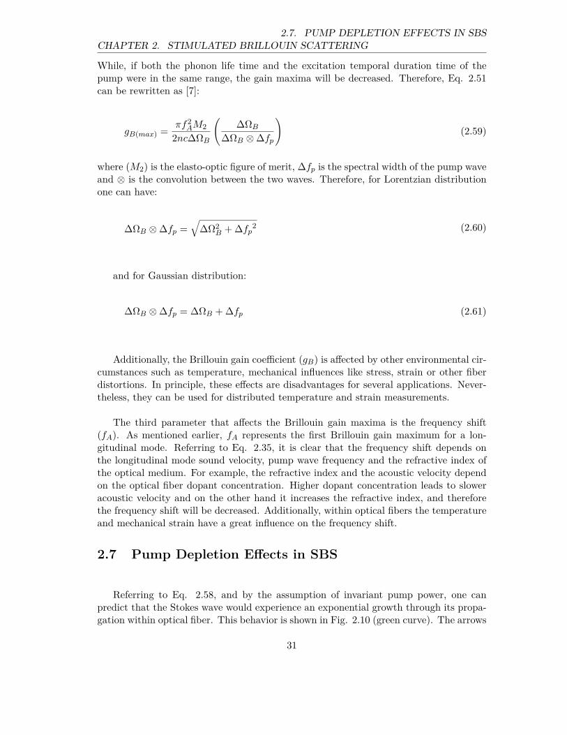
CHAPTER 2. STIMULATED BRILLOUIN SCATTERING2.7. PUMP DEPLETION EFFECTS IN SBS
While, if both the phonon life time and the excitation temporal duration time of thepump were in the same range, the gain maxima will be decreased. Therefore, Eq. 2.51can be rewritten as [7]:
gB(max) =πf2
AM2
2nc∆ΩB
(∆ΩB
∆ΩB ⊗ ∆fp
)(2.59)
where (M2) is the elasto-optic figure of merit, ∆fp is the spectral width of the pump waveand ⊗ is the convolution between the two waves. Therefore, for Lorentzian distributionone can have:
∆ΩB ⊗ ∆fp =√
∆Ω2B + ∆fp
2 (2.60)
and for Gaussian distribution:
∆ΩB ⊗ ∆fp = ∆ΩB + ∆fp (2.61)
Additionally, the Brillouin gain coefficient (gB) is affected by other environmental cir-cumstances such as temperature, mechanical influences like stress, strain or other fiberdistortions. In principle, these effects are disadvantages for several applications. Never-theless, they can be used for distributed temperature and strain measurements.
The third parameter that affects the Brillouin gain maxima is the frequency shift(fA). As mentioned earlier, fA represents the first Brillouin gain maximum for a lon-gitudinal mode. Referring to Eq. 2.35, it is clear that the frequency shift depends onthe longitudinal mode sound velocity, pump wave frequency and the refractive index ofthe optical medium. For example, the refractive index and the acoustic velocity dependon the optical fiber dopant concentration. Higher dopant concentration leads to sloweracoustic velocity and on the other hand it increases the refractive index, and thereforethe frequency shift will be decreased. Additionally, within optical fibers the temperatureand mechanical strain have a great influence on the frequency shift.
2.7 Pump Depletion Effects in SBS
Referring to Eq. 2.58, and by the assumption of invariant pump power, one canpredict that the Stokes wave would experience an exponential growth through its propa-gation within optical fiber. This behavior is shown in Fig. 2.10 (green curve). The arrows
31
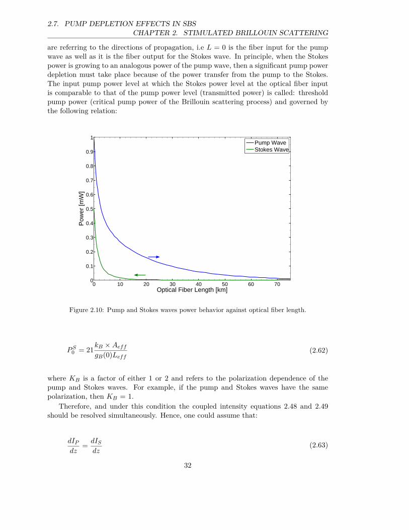
2.7. PUMP DEPLETION EFFECTS IN SBSCHAPTER 2. STIMULATED BRILLOUIN SCATTERING
are referring to the directions of propagation, i.e L = 0 is the fiber input for the pumpwave as well as it is the fiber output for the Stokes wave. In principle, when the Stokespower is growing to an analogous power of the pump wave, then a significant pump powerdepletion must take place because of the power transfer from the pump to the Stokes.The input pump power level at which the Stokes power level at the optical fiber inputis comparable to that of the pump power level (transmitted power) is called: thresholdpump power (critical pump power of the Brillouin scattering process) and governed bythe following relation:
0 10 20 30 40 50 60 700
0.1
0.2
0.3
0.4
0.5
0.6
0.7
0.8
0.9
1
Optical Fiber Length [km]
Pow
er [m
W]
Pump WaveStokes Wave
Figure 2.10: Pump and Stokes waves power behavior against optical fiber length.
PS0 = 21
kB ×Aeff
gB(0)Leff(2.62)
where KB is a factor of either 1 or 2 and refers to the polarization dependence of thepump and Stokes waves. For example, if the pump and Stokes waves have the samepolarization, then KB = 1.
Therefore, and under this condition the coupled intensity equations 2.48 and 2.49should be resolved simultaneously. Hence, one could assume that:
dIP
dz=dIS
dz(2.63)
32

CHAPTER 2. STIMULATED BRILLOUIN SCATTERING2.7. PUMP DEPLETION EFFECTS IN SBS
and therefore:
IP (z) = IS(z) + C (2.64)
where C is the integration constant which is related to the boundary conditions [1].Hence, Eq. 2.49 can be rewritten as:
dIS
IS(IS + C)= −gBdz (2.65)
After integration Eq. 2.65 will be:
∫ IS(z)
IS(0)
dIS
IS(IS + C)= −
∫ z
0gBdz
′ (2.66)
then:
ln
IS(z)[IS(0) + C]
IS(0)[IS(z) + C]
= −gBCz (2.67)
In principle, the pump power value IP (0) is known, therefore the integration constantC can be expressed as (C = IP (0) − IS(0)). Hence, Eq. 2.67 can be solved algebraicallyfor the Stokes power at any position of the optical fiber (z) as:
IS(z) =IS(0)[IP (0) − IS(0)]
IP (0) exp (gBz[IP (0) − IS(0)]) − IS(0)(2.68)
Referring to Eq. 2.64, the pump power at (z) position of the optical fiber can be writtenby means of the power conservation law as:
IP (z) = IS(z) + IP (0) − IS(0) (2.69)
Now one can find the intensity values for both the pump and Stokes at z, i.e. thespatial distribution in terms of the given boundary values at the input of the opticalfiber IP (0) and IS(0). Referring to Fig. 2.11, the boundary values IP (0) and IS(L) could
33
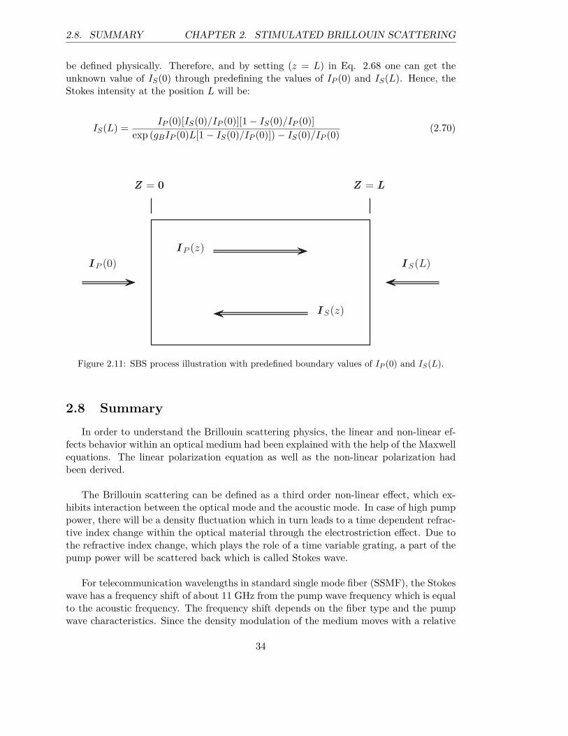
2.8. SUMMARY CHAPTER 2. STIMULATED BRILLOUIN SCATTERING
be defined physically. Therefore, and by setting (z = L) in Eq. 2.68 one can get theunknown value of IS(0) through predefining the values of IP (0) and IS(L). Hence, theStokes intensity at the position L will be:
IS(L) =IP (0)[IS(0)/IP (0)][1 − IS(0)/IP (0)]
exp (gBIP (0)L[1 − IS(0)/IP (0)]) − IS(0)/IP (0)(2.70)
I P (0) I S(L)
I P (z)
I S(z)
Z = LZ = 0
Figure 2.11: SBS process illustration with predefined boundary values of IP (0) and IS(L).
2.8 Summary
In order to understand the Brillouin scattering physics, the linear and non-linear ef-fects behavior within an optical medium had been explained with the help of the Maxwellequations. The linear polarization equation as well as the non-linear polarization hadbeen derived.
The Brillouin scattering can be defined as a third order non-linear effect, which ex-hibits interaction between the optical mode and the acoustic mode. In case of high pumppower, there will be a density fluctuation which in turn leads to a time dependent refrac-tive index change within the optical material through the electrostriction effect. Due tothe refractive index change, which plays the role of a time variable grating, a part of thepump power will be scattered back which is called Stokes wave.
For telecommunication wavelengths in standard single mode fiber (SSMF), the Stokeswave has a frequency shift of about 11 GHz from the pump wave frequency which is equalto the acoustic frequency. The frequency shift depends on the fiber type and the pumpwave characteristics. Since the density modulation of the medium moves with a relative
34
CHAPTER 2. STIMULATED BRILLOUIN SCATTERING 2.8. SUMMARY
velocity to the pump and in its direction, the Stokes wave is down shifted in frequency.Therefore, both pump and Stokes waves are counter propagating through the opticalmedium.
The governing equations for the pump and Stokes waves had been derived in addi-tion to the Brillouin gain parameter. The Brillouin gain coefficient linewidth dependson many factors like: the optical medium characteristics, the temperature as well as theoptical fiber core diameter and the spectral width of the pump wave. Usually for a silicaoptical fiber within room temperature the Brillouin gain coefficient has a natural gainlinewidth of about 35 MHz. However, by increasing the pump power the bandwidthdecreases.
At a certain pump power level, the scattering starts to be stimulated. Therefore,the Stokes wave growths up exponentially within the optical medium. That specificpump power level is called threshold and governed by the gain coefficient. The Brillouinscattering effect has the lowest non-linear threshold pump power. The threshold pumppower level depends mainly on the fiber length, by which it decreases with increasingfiber length. However, it will reach a fixed value after a length that could be definedby the fiber attenuation depending on the fiber effective length behavior. The thresholdpower level limits the input pump power for a lot of applications. However, one can getrid of this limitation by using a higher bandwidth transmitted signal than the intrinsicBrillouin gain bandwidth and therefore increasing the SBS threshold.
35

2.8. SUMMARY CHAPTER 2. STIMULATED BRILLOUIN SCATTERING
36
Chapter 3
SBS Gain Enhancement Based onIntegrated Silicon Photonics
3.1 Introduction
As explained in the previous chapter, the Stimulated Brillouin Scattering (SBS) is athird-order non-linear optical process by which optical photons are coupled to acousticphonons, i.e. two optical modes (the pump and the Stokes ) are coupled through anelastic mode. The SBS has unique properties, which makes it very attractive for manyapplications developed in the last few years. For optical telecommunications especiallythe alteration of the group velocity (Slow- and Fast Light), Quasi Light Storage (QLS)[41], microwave photonics and Ultrahigh-Resolution Spectroscopy (URS) are very impor-tant [7, 1, 2]. In principle, in optical fibers the SBS is initiated by electrostriction, whichmakes the effect rather low and requires kilometers of fiber to be effective and sufficient.However, within the nano-scale this role can be broken down, since tremendous pressureforces can form new SBS non-linearities [18].
In silicon-on-insulator (SOI) based sub-wavelength waveguides a combination of elec-trostriction and radiation pressure can lead to an enhancement of the SBS effect byseveral orders of magnitude. Therefore, such type of nano-waveguides based chips havethe potential to effectively store optical packets, measure optical spectra with ultrahighresolution, or can be the building blocks of microwave photonics [42].
In principle, SOI technology refers to the utilization of a layered silicon–insulator–silicon substrate in place of conventional silicon substrates in semiconductor utilizationlike microelectronics. The main difference between SOI-based devices and conventionalsilicon-built devices is that the silicon junction is above an electrical insulator. For ex-ample, silicon dioxide or sapphire devices which are called silicon on sapphire (SOS).The selection of insulator type depends mainly on the desired application. For example,sapphire being used for high-performance radio frequency (RF) and radiation-sensitiveapplications. Additionally, silicon dioxide is used for diminished short channel effects in
37

3.2. SILICON CRYSTALLINE STRUCTURECHAPTER 3. SBS GAIN ENHANCEMENT BASED ON INTEGRATED SILICON
PHOTONICS
microelectronics devices [43]. However, the insulating layer and topmost silicon layer alsocan be different according to the desired application [44].
In RF applications for instance, the development of an SOI fabrication technologyusing a standard 0.5 µm CMOS node and an enhanced sapphire substrate had been done.The invention of silicon on sapphire (SOS) fabrication is widely used in high-performanceRF applications, since its intrinsic benefits of the insulating sapphire substrate which al-lows high isolation, high linearity and electro-static discharge. Additionally, SOI wafersare mainly used for silicon photonics fabrications. For example, nowadays the crystallinesilicon layer on insulator is used for optical nano-waveguides fabrication as well as otherpassive optical devices for integrated optics. In principle, the crystalline silicon layer issandwiched between the buried insulator and top cladding of air (or Silicon oxide or anyother low refractive index material). Therefore, this enables propagation of electromag-netic waves in the waveguides on the basis of total internal reflection.
Having the fact, that within SBS process two optical modes are coupled throughan elastic mode, therefore at a certain beat frequency (simultaneously frequency andphase matched) a dynamic optical force is generated through the interference betweenthe pump and Stokes waves. Hence, a mechanical oscillation takes place in the nano-waveguide. Because of the transverse dimensions of the silicon nano-waveguide, bothwaves are greatly confined as discrete sets of Eigen-modes. The optical forces inside thenano-waveguide can be divided into two types: electrostriction and radiation forces andeach type has two kinds: bulk and boundary forces.
This chapter is organized as follows: the silicon crystalline structure as well as thesilicon lattice structure will be explained. The two-photon absorption non-linearity willbe presented in order to calculate the maximum launchable input pump power for theSOI waveguide. Two kinds of forces: electrostriction and radiation will be studied. Foreach force two types will be investigated: body and pressure.The Brillouin gain and the predicted Stokes wave power will be calculated in terms of theopto-mechanical forces and the elastic waveguide deformation. Two kinds of waveguideswill be studied: strip and rib, each two structures will be investigated. Simulation resultswill be presented for rectangular SOI based strip and rib nano-waveguides, showing thevery high potential of this new approach.
3.2 Silicon Crystalline Structure
3.2.1 Silicon Lattice
Silicon has a cubic crystalline centro-symmetric structure. In general, the crystalseventually terminate at a surface since they are not infinitely large. Semiconductor de-vices are fabricated at or near a surface; therefore the surface properties give an indicationabout the device characteristics. It is interesting to describe these surfaces in terms ofthe lattice. Assuming a general three dimensional unit cell shown in Fig. 3.1 with wavevectors a, b and c.
38
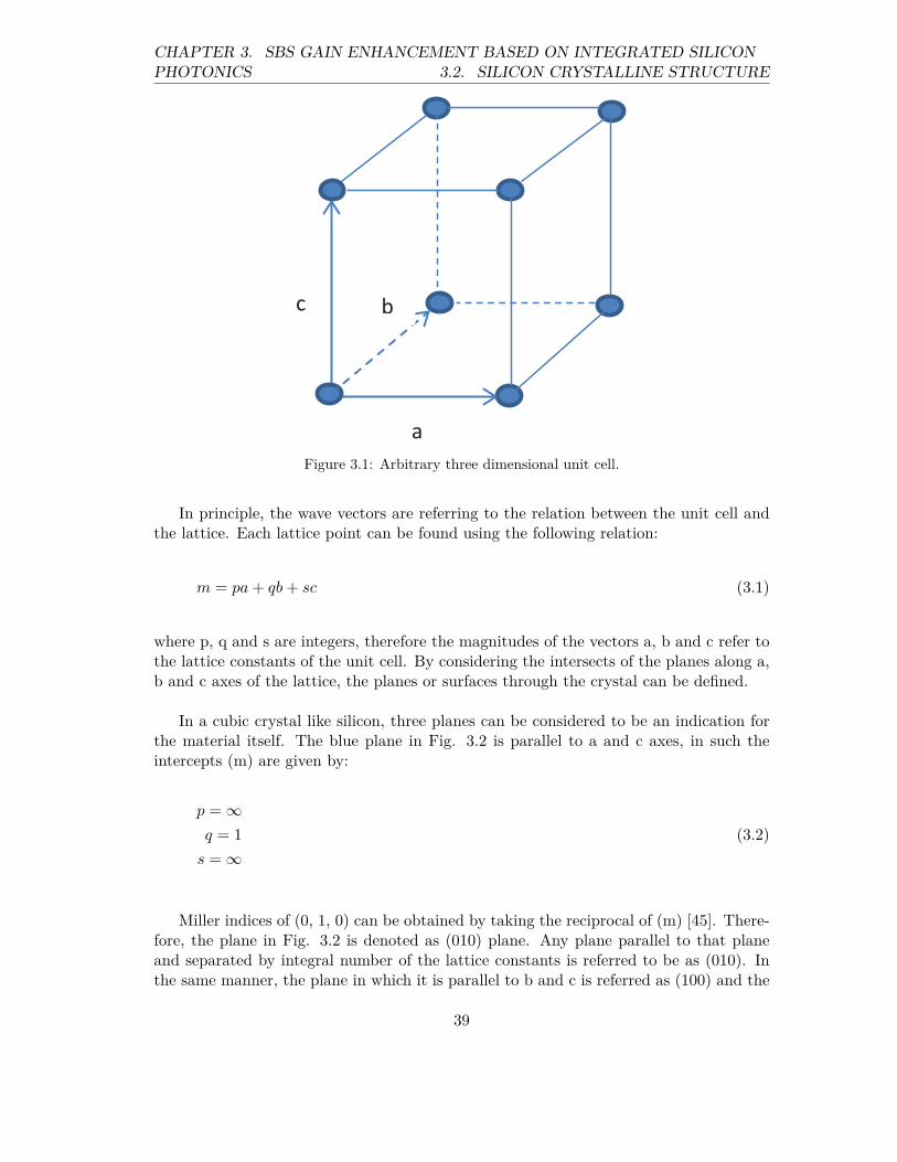
CHAPTER 3. SBS GAIN ENHANCEMENT BASED ON INTEGRATED SILICONPHOTONICS 3.2. SILICON CRYSTALLINE STRUCTURE
a
b c
Figure 3.1: Arbitrary three dimensional unit cell.
In principle, the wave vectors are referring to the relation between the unit cell andthe lattice. Each lattice point can be found using the following relation:
m = pa+ qb+ sc (3.1)
where p, q and s are integers, therefore the magnitudes of the vectors a, b and c refer tothe lattice constants of the unit cell. By considering the intersects of the planes along a,b and c axes of the lattice, the planes or surfaces through the crystal can be defined.
In a cubic crystal like silicon, three planes can be considered to be an indication forthe material itself. The blue plane in Fig. 3.2 is parallel to a and c axes, in such theintercepts (m) are given by:
p = ∞q = 1
s = ∞(3.2)
Miller indices of (0, 1, 0) can be obtained by taking the reciprocal of (m) [45]. There-fore, the plane in Fig. 3.2 is denoted as (010) plane. Any plane parallel to that planeand separated by integral number of the lattice constants is referred to be as (010). Inthe same manner, the plane in which it is parallel to b and c is referred as (100) and the
39
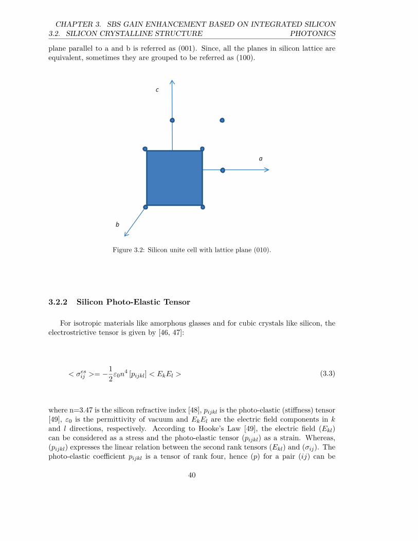
3.2. SILICON CRYSTALLINE STRUCTURECHAPTER 3. SBS GAIN ENHANCEMENT BASED ON INTEGRATED SILICON
PHOTONICS
plane parallel to a and b is referred as (001). Since, all the planes in silicon lattice areequivalent, sometimes they are grouped to be referred as (100).
b
a
c
Figure 3.2: Silicon unite cell with lattice plane (010).
3.2.2 Silicon Photo-Elastic Tensor
For isotropic materials like amorphous glasses and for cubic crystals like silicon, theelectrostrictive tensor is given by [46, 47]:
< σesij >= −1
2ε0n
4 [pijkl] < EkEl > (3.3)
where n=3.47 is the silicon refractive index [48], pijkl is the photo-elastic (stiffness) tensor[49], ε0 is the permittivity of vacuum and EkEl are the electric field components in kand l directions, respectively. According to Hooke’s Law [49], the electric field (Ekl)can be considered as a stress and the photo-elastic tensor (pijkl) as a strain. Whereas,(pijkl) expresses the linear relation between the second rank tensors (Ekl) and (σij). Thephoto-elastic coefficient pijkl is a tensor of rank four, hence (p) for a pair (ij) can be
40

CHAPTER 3. SBS GAIN ENHANCEMENT BASED ON INTEGRATED SILICONPHOTONICS 3.2. SILICON CRYSTALLINE STRUCTURE
written as [49]:
pij =
p11 p12 p13 p14 p15 p16
p21 p22 p23 p24 p25 p26
p31 p32 p33 p34 p35 p36
p41 p42 p43 p44 p45 p46
p51 p52 p53 p54 p55 p56
p61 p62 p63 p64 p65 p66
(3.4)
Since the tensors Ekl and σij are symmetric, the photo-elastic coefficients are unaf-fected when either the first two or the last two indices are interchanged, Hence:
pijkl = pjikl
pijkl = pijlk
(3.5)
According to that symmetry, pijkl is symmetric about its main diagonal and therefore,Eq. 3.4 can be rewritten as:
pij =
p11 p12 p13 p14 p15 p16
p12 p22 p23 p24 p25 p26
p13 p23 p33 p34 p35 p36
p14 p24 p34 p44 p45 p46
p15 p25 p35 p45 p55 p56
p16 p26 p36 p46 p56 p66
(3.6)
Since, silicon has a cubic crystalline symmetric structure and according to the earliersilicon lattice description by which silicon is symmetric with respect to x=0, y=0 andz=0, thus pij is zero if it contains odd number of certain components. Therefore, pij canbe rewritten as:
pij =
p11 p12 p13 0 0 0p12 p22 p23 0 0 0p13 p23 p33 0 0 00 0 0 p44 0 00 0 0 0 p55 00 0 0 0 0 p66
(3.7)
Referring to the silicon parameters as: refractive index n = 3.47, Young’s modulusE = 170×109 Pa and Poisson’s ration ν = 0.28. The photo-elastic coefficients would
41

3.3. TWO-PHOTON ABSORPTION (TPA) IN SILICONCHAPTER 3. SBS GAIN ENHANCEMENT BASED ON INTEGRATED SILICON
PHOTONICS
be: p11 = p22 = p33 = −0.09, p12 = p13 = p21 = p23 = p31 = p32 = 0.017 andp44 = p55 = p66 = −0.051 [49]. These parameters had been used to achieve the simulationresults, presented in the next sections.
3.3 Two-Photon Absorption (TPA) in Silicon
Due to the high index contrast between the silicon core and silica cladding, siliconwaveguides allow strong optical confinement and large effective non-linearity. Therefore,it facilitates low cost chip-scale demonstration of all-optical non-linear functional devicesat low pump powers.
In SOI waveguides the non-linear Kerr parameter can scale up to 7×10³ (W−1∗m−1)[50]. Hence, it is about three orders of magnitude higher than the non-linearity in highlynon-linear optical fibers. Additionally, within SOI waveguides there are a variety of op-tical non-linear effects since they are generated from the interaction of the optical fieldwith phonons and electrons.
Two-Photon Absorption (TPA) is a third order non-linear process. It is one of themost effective non-linear effects in SOI waveguides, by which it is dominated in highoptical intensities. Additionally, it can be assumed as a fundamental limitation for theSOI devices. Silicon has an indirect band gap of 1.12 eV. Therefore, a single photon isnot enough to excite an electron from the Valence band (Vb) to the Conduction band(Cb) as illustrated in Fig. 3.3.
Vb
Cb
Hole
Electron
Band gap=1.12 eV
Figure 3.3: Indirect band gap illustration of silicon.
In principle, TPA involves the simultaneous absorption of two photons during theexcitation of one electron from Vb to Cb. Since silicon has an indirect bad gap of1.12 eV, the sum of the energies of the two absorbed phonons should exceed 1.12 eV.
42
CHAPTER 3. SBS GAIN ENHANCEMENT BASED ON INTEGRATED SILICONPHOTONICS 3.4. ELECTROSTRICTION FORCES
TPA excitations are absorbing, since energetically they correspond to an excitation ofan electron from the Vb to the Cb. Therefore, TPA generates free carriers in the Cbin which they act as sources for Free Carrier Absorption (FCA) and Free Carrier Index(FCI). Thus, the long lifetime of the free carriers in the Cb leads to long-lasting FCAand FCI effects. The results is a speed down of SOI devices. The TPA loss is governedby the following intensity dependent relation:
dI
dx= −βI2 (3.8)
where x is the propagation direction, β is the TPA coefficient and I is the optical intensityin the waveguide. One can use the Drude model to describe the TPA-induced free carrierabsorption loss as [51]:
∆αF CA∼= 6.04e−18λ2
pβI2(τeff/2Ep) (3.9)
where λp denotes the pump wavelength in nm, τeff is the effective carrier lifetime (carrierlifetime is the average time it takes for a minority carrier to recombine) and Ep is thephoton energy. The TPA parameter (β) was measured by many groups and it is varyingbetween 0.4 to 1.5 cm/GW [52]. If the two photons have the same frequency, then thisis referred as degenerate TPA (two photons from the Pump or the Stokes wave). Non-degenerate TPA takes place when the two photons have different frequencies (one photonfrom the pump and one from the Stokes wave). According to [53], the TPA thresholdinput power for the same SOI waveguide type and dimensions that was in the simulationshere is 30 mW.
Many methods can be found in the literature to reduce the effect of the FCA, suchas:
1. Operation at low pump power.
2. Increase the device length.
3. Using a pulsed pump power laser.
4. Sweeping out the free carriers from the optical mode using a transverse p-n junctionstructure.
3.4 Electrostriction Forces
The forces are generated through the SBS process by the interaction of the Pumpwave (Epe
i(kpx−ωpt)) and the Stokes wave (Esei(−ksx−ωst)), this results in a beat wave
with a frequency (Ω = ωp − ωs) and a wave vector (kA = kP − kS), as described in theprevious chapter. In principle, the maximum SBS gain value is determined by the elastic
43

3.4. ELECTROSTRICTION FORCESCHAPTER 3. SBS GAIN ENHANCEMENT BASED ON INTEGRATED SILICON
PHOTONICS
wave damping [18]. At resonance, the peak elastic displacement velocity is proportionalto the phononic quality factor (Q) and the optical force value. Therefore, within sim-ulations and depending on the silicon damping limit for the frequency range of interest[54], one can assume a frequency-independent quality factor of Q=1000 as a phononicproperty (energy loss in the resonator) for all elastic modes, where [49, 55, 56]:
Q = 2πmaximum energy stored during a period of oscillation
energy lost during a period of oscillation(3.10)
The pump and Stokes waves can be launched in the same direction for forward SBS(FSBS) and in opposite direction for backward SBS (BSBS). In FSBS, the generatedforces excite standing-wave elastic modes, while in BSBS traveling-wave elastic modesare excited. The high optical intensity in the waveguide leads to a compression of thematerial in that region, so that an electrostriction force is generated in the bulk, whilethe electrostriction pressure is generated from the discontinuities of the optical intensitiesand photo-elastic coefficients at the boundaries. The parametric conversion between thepump and Stokes waves is described by Eq. 2.56. Instead, here we used x rather than z.
Although, the Brillouin gain gB can be calculated from Eq. 2.50 in terms of valuesof the maximum gain ΩB(0), frequency shift ∆Ω and linewidth ∆ΩB. One can get theBrillouin gain gB from the following relation [16]:
gB = 2
(ωs
Ω
)∫
wgRe[fn(x, y)un(x, y)
]dA (3.11)
where fn are the total optical forces, un is the elastic Eigen mode deformation andfn(x, y)un(x, y) is the overlap integral between the forces and the elastic deformation.For the bulk forces the integration is taken over the waveguide cross section while for thepressure forces it is taken over the boundaries.
In principle, the electrostriction forces can be derived from the electrostriction tensor.Therefore, the total electric field of the waveguide system will be substituted in Eq. 3.3.The total electric field within the waveguide system is:
E =Epe
i(kpx−ωpt) + Esei(−ksx−ωst)
2+ C.C. (3.12)
then Eq. 3.3 can be rewritten as:
< σesij >= −1
4ε0n
4 [pijkl] (EpkE∗
sl + EplE∗
sk) (3.13)
44
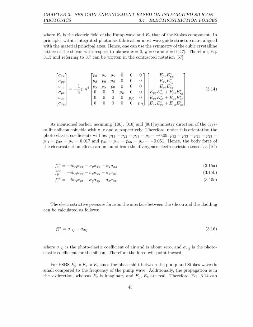
CHAPTER 3. SBS GAIN ENHANCEMENT BASED ON INTEGRATED SILICONPHOTONICS 3.4. ELECTROSTRICTION FORCES
where Ep is the electric field of the Pump wave and Es that of the Stokes component. Inprinciple, within integrated photonics fabrication most waveguide structures are alignedwith the material principal axes. Hence, one can use the symmetry of the cubic crystallinelattice of the silicon with respect to planes: x = 0, y = 0 and z = 0 [47]. Therefore, Eq.3.13 and referring to 3.7 can be written in the contracted notation [57]:
σxx
σyy
σzz
σyz
σxz
σxy
= −1
4ε0n
4
p0 pS pS 0 0 0pS p0 pS 0 0 0pS pS p0 0 0 00 0 0 pR 0 00 0 0 0 pR 00 0 0 0 0 pR
EpxE∗
sx
EpyE∗
sy
EpzE∗
sz
EpyE∗
sz + EpzE∗
sy
EpxE∗
sz + EpzE∗
sx
EpxE∗
sy + EpyE∗
sx
(3.14)
As mentioned earlier, assuming [100], [010] and [001] symmetry direction of the crys-talline silicon coincide with x, y and z, respectively. Therefore, under this orientation thephoto-elastic coefficients will be: p11 = p22 = p33 = p0 = −0.09, p12 = p13 = p21 = p23 =p31 = p32 = pS = 0.017 and p44 = p55 = p66 = pR = −0.051. Hence, the body force ofthe electrostriction effect can be found from the divergence electrostriction tensor as [16]:
fesx = −ikAσxx − σyσxy − σzσxz (3.15a)
fesy = −ikAσxy − σyσyy − σzσyz (3.15b)
fesz = −ikAσxz − σyσzy − σzσxz (3.15c)
The electrostrictive pressure force on the interface between the silicon and the claddingcan be calculated as follows:
fesi = σ1ij − σ2ij (3.16)
where σ1ij is the photo-elastic coefficient of air and is about zero, and σ2ij is the photo-elastic coefficient for the silicon. Therefore the force will point inward.
For FSBS Ep ≈ Es ≈ E, since the phase shift between the pump and Stokes waves issmall compared to the frequency of the pump wave. Additionally, the propagation is inthe x-direction, whereas Ex is imaginary and Ey, Ez are real. Therefore, Eq. 3.14 can
45

3.5. RADIATION FORCESCHAPTER 3. SBS GAIN ENHANCEMENT BASED ON INTEGRATED SILICON
PHOTONICS
be rewritten as:
σxx
σyy
σzz
σyz
σxz
σxy
= −1
4ε0n
4
p0 pS pS 0 0 0pS p0 pS 0 0 0pS pS p0 0 0 00 0 0 pR 0 00 0 0 0 pR 00 0 0 0 0 pR
|Ex|2|Ey|2|Ez|2
2Re(EyEz)00
(3.17)
Therefore, Eq. 3.15 will be rewritten as:
fesx = 0 (3.18a)
fesy = σyσyy − σzσyz (3.18b)
fesz = σyσzy − σzσxz (3.18c)
Within BSBS kA = 2kp and Ep = E, Es = E∗, therefore Eq. 3.14 can be expressedas:
σxx
σyy
σzz
σyz
σxz
σxy
= −1
4ε0n
4
p0 pS pS 0 0 0pS p0 pS 0 0 0pS pS p0 0 0 00 0 0 pR 0 00 0 0 0 pR 00 0 0 0 0 pR
E2x
E2y
E2z
2EyEz
2ExEz
2ExEy
(3.19)
Additionally, it can be shown that the electrostrictive body force is both transverseand longitudinal since Eq. 3.15 has a non-zero component.
3.5 Radiation Forces
In principle, both body and radiation pressure forces can be derived from MaxwellsStress Tensor (MST) which is [58]:
Tij = ε0ε(x, y)
[EiEj − 1
2δij |E|2
]+ µ0µ
[HiHj − 1
2δij |H|2
](3.20)
where ε0 and ε are the vacuum dielectric and relative dielectric permittivity, µ0 and µ are
46
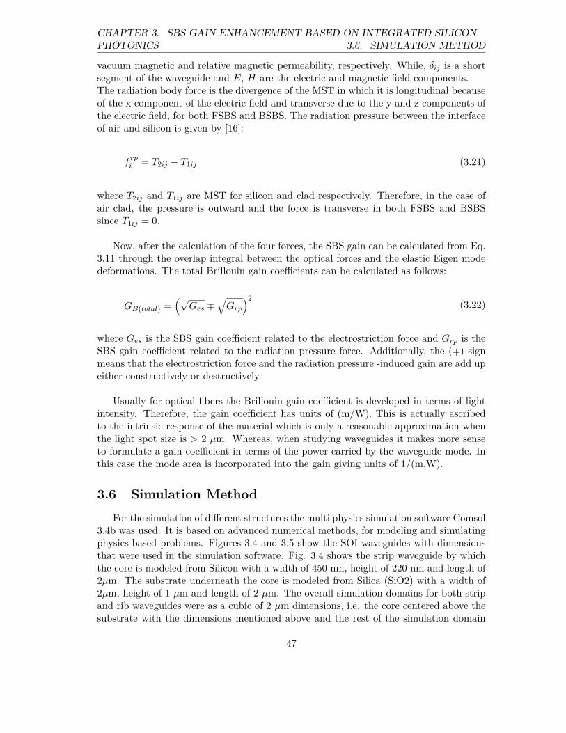
CHAPTER 3. SBS GAIN ENHANCEMENT BASED ON INTEGRATED SILICONPHOTONICS 3.6. SIMULATION METHOD
vacuum magnetic and relative magnetic permeability, respectively. While, δij is a shortsegment of the waveguide and E, H are the electric and magnetic field components.The radiation body force is the divergence of the MST in which it is longitudinal becauseof the x component of the electric field and transverse due to the y and z components ofthe electric field, for both FSBS and BSBS. The radiation pressure between the interfaceof air and silicon is given by [16]:
f rpi = T2ij − T1ij (3.21)
where T2ij and T1ij are MST for silicon and clad respectively. Therefore, in the case ofair clad, the pressure is outward and the force is transverse in both FSBS and BSBSsince T1ij = 0.
Now, after the calculation of the four forces, the SBS gain can be calculated from Eq.3.11 through the overlap integral between the optical forces and the elastic Eigen modedeformations. The total Brillouin gain coefficients can be calculated as follows:
GB(total) =(√
Ges ∓√Grp
)2(3.22)
where Ges is the SBS gain coefficient related to the electrostriction force and Grp is theSBS gain coefficient related to the radiation pressure force. Additionally, the (∓) signmeans that the electrostriction force and the radiation pressure -induced gain are add upeither constructively or destructively.
Usually for optical fibers the Brillouin gain coefficient is developed in terms of lightintensity. Therefore, the gain coefficient has units of (m/W). This is actually ascribedto the intrinsic response of the material which is only a reasonable approximation whenthe light spot size is > 2 µm. Whereas, when studying waveguides it makes more senseto formulate a gain coefficient in terms of the power carried by the waveguide mode. Inthis case the mode area is incorporated into the gain giving units of 1/(m.W).
3.6 Simulation Method
For the simulation of different structures the multi physics simulation software Comsol3.4b was used. It is based on advanced numerical methods, for modeling and simulatingphysics-based problems. Figures 3.4 and 3.5 show the SOI waveguides with dimensionsthat were used in the simulation software. Fig. 3.4 shows the strip waveguide by whichthe core is modeled from Silicon with a width of 450 nm, height of 220 nm and length of2µm. The substrate underneath the core is modeled from Silica (SiO2) with a width of2µm, height of 1 µm and length of 2 µm. The overall simulation domains for both stripand rib waveguides were as a cubic of 2 µm dimensions, i.e. the core centered above thesubstrate with the dimensions mentioned above and the rest of the simulation domain
47
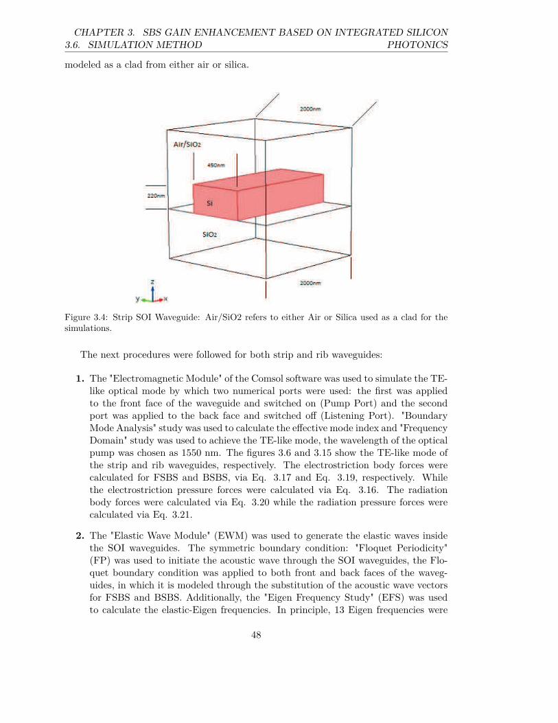
3.6. SIMULATION METHODCHAPTER 3. SBS GAIN ENHANCEMENT BASED ON INTEGRATED SILICON
PHOTONICS
modeled as a clad from either air or silica.
Figure 3.4: Strip SOI Waveguide: Air/SiO2 refers to either Air or Silica used as a clad for thesimulations.
The next procedures were followed for both strip and rib waveguides:
1. The "Electromagnetic Module" of the Comsol software was used to simulate the TE-like optical mode by which two numerical ports were used: the first was appliedto the front face of the waveguide and switched on (Pump Port) and the secondport was applied to the back face and switched off (Listening Port). "BoundaryMode Analysis" study was used to calculate the effective mode index and "FrequencyDomain" study was used to achieve the TE-like mode, the wavelength of the opticalpump was chosen as 1550 nm. The figures 3.6 and 3.15 show the TE-like mode ofthe strip and rib waveguides, respectively. The electrostriction body forces werecalculated for FSBS and BSBS, via Eq. 3.17 and Eq. 3.19, respectively. Whilethe electrostriction pressure forces were calculated via Eq. 3.16. The radiationbody forces were calculated via Eq. 3.20 while the radiation pressure forces werecalculated via Eq. 3.21.
2. The "Elastic Wave Module" (EWM) was used to generate the elastic waves insidethe SOI waveguides. The symmetric boundary condition: "Floquet Periodicity"(FP) was used to initiate the acoustic wave through the SOI waveguides, the Flo-quet boundary condition was applied to both front and back faces of the waveg-uides, in which it is modeled through the substitution of the acoustic wave vectorsfor FSBS and BSBS. Additionally, the "Eigen Frequency Study" (EFS) was usedto calculate the elastic-Eigen frequencies. In principle, 13 Eigen frequencies were
48
CHAPTER 3. SBS GAIN ENHANCEMENT BASED ON INTEGRATED SILICONPHOTONICS 3.7. 220X450 NM SILICON WAVEGUIDE
Figure 3.5: Rib SOI Waveguide: Air/SiO2 refers to either Air or Silica used as a clad in thesimulations.
achieved by searching around 13 GHz for 13 Eigen frequencies: as a number offrequencies. Additionally, the quality factor (Q = 1000) was used for all the elasticEigen-modes [47].
3. The "MATLAB Life Link Module" was used as a client with COMSOL server tosimulate the SBS gain coefficients via Eq. 3.11. The gain profiles had been plottedversus the achieved Eigen frequencies.
3.7 220x450 nm Silicon Waveguide
First a silicon waveguide with a length of 2 µm, a height of 220 nm and a widthof 450 nm had been simulated. Two kinds of waveguides were simulated (strip and ribwaveguides) and for each kind two cases were investigated, silicon core on silica substratewith air cladding and silicon core on silica substrate with silica cladding. The refractiveindex of silicon for 1550 nm wavelength was chosen as n=3.47 and for silica as n=1.45.
A strip waveguide is a rectangular waveguide in which the core is made from siliconand the substrate from silica, the core is based directly on the substrate without a slab asshown in Fig. 3.4. The clad is made from either air or silica. Whereas, a rib waveguideis just like the strip waveguide but it consists of a slab of 50 nm between the silicon coreand the substrate and this slab is made of silicon. Therefore, the core height will be220 nm as shown in Fig. 3.5. The bold red interfaces refer to the separations betweenmaterials.
49
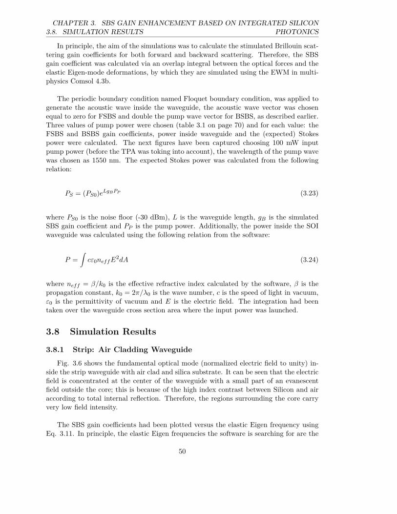
3.8. SIMULATION RESULTSCHAPTER 3. SBS GAIN ENHANCEMENT BASED ON INTEGRATED SILICON
PHOTONICS
In principle, the aim of the simulations was to calculate the stimulated Brillouin scat-tering gain coefficients for both forward and backward scattering. Therefore, the SBSgain coefficient was calculated via an overlap integral between the optical forces and theelastic Eigen-mode deformations, by which they are simulated using the EWM in multi-physics Comsol 4.3b.
The periodic boundary condition named Floquet boundary condition, was applied togenerate the acoustic wave inside the waveguide, the acoustic wave vector was chosenequal to zero for FSBS and double the pump wave vector for BSBS, as described earlier.Three values of pump power were chosen (table 3.1 on page 70) and for each value: theFSBS and BSBS gain coefficients, power inside waveguide and the (expected) Stokespower were calculated. The next figures have been captured choosing 100 mW inputpump power (before the TPA was toking into account), the wavelength of the pump wavewas chosen as 1550 nm. The expected Stokes power was calculated from the followingrelation:
PS = (PS0)eLgBPP (3.23)
where PS0 is the noise floor (-30 dBm), L is the waveguide length, gB is the simulatedSBS gain coefficient and PP is the pump power. Additionally, the power inside the SOIwaveguide was calculated using the following relation from the software:
P =
∫cε0neffE
2dA (3.24)
where neff = β/k0 is the effective refractive index calculated by the software, β is thepropagation constant, k0 = 2π/λ0 is the wave number, c is the speed of light in vacuum,ε0 is the permittivity of vacuum and E is the electric field. The integration had beentaken over the waveguide cross section area where the input power was launched.
3.8 Simulation Results
3.8.1 Strip: Air Cladding Waveguide
Fig. 3.6 shows the fundamental optical mode (normalized electric field to unity) in-side the strip waveguide with air clad and silica substrate. It can be seen that the electricfield is concentrated at the center of the waveguide with a small part of an evanescentfield outside the core; this is because of the high index contrast between Silicon and airaccording to total internal reflection. Therefore, the regions surrounding the core carryvery low field intensity.
The SBS gain coefficients had been plotted versus the elastic Eigen frequency usingEq. 3.11. In principle, the elastic Eigen frequencies the software is searching for are the
50
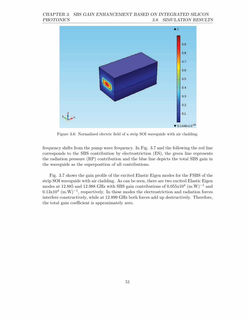
CHAPTER 3. SBS GAIN ENHANCEMENT BASED ON INTEGRATED SILICONPHOTONICS 3.8. SIMULATION RESULTS
Figure 3.6: Normalized electric field of a strip SOI waveguide with air cladding.
frequency shifts from the pump wave frequency. In Fig. 3.7 and the following the red linecorresponds to the SBS contribution by electrostriction (ES), the green line representsthe radiation pressure (RP) contribution and the blue line depicts the total SBS gain inthe waveguide as the superposition of all contributions.
Fig. 3.7 shows the gain profile of the excited Elastic Eigen modes for the FSBS of thestrip SOI waveguide with air cladding. As can be seen, there are two excited Elastic Eigenmodes at 12.885 and 12.988 GHz with SBS gain contributions of 0.055x10⁴ (m.W)−1 and0.13x104 (m.W)−1, respectively. In these modes the electrostriction and radiation forcesinterfere constructively, while at 12.899 GHz both forces add up destructively. Therefore,the total gain coefficient is approximately zero.
51
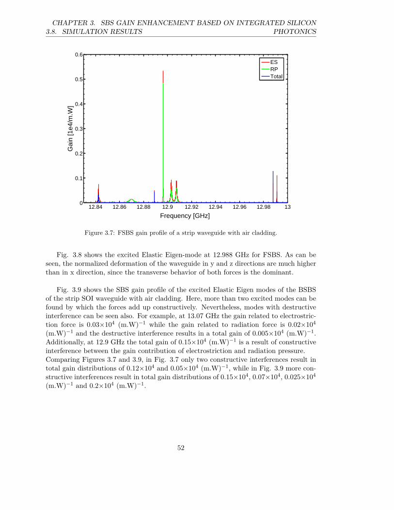
3.8. SIMULATION RESULTSCHAPTER 3. SBS GAIN ENHANCEMENT BASED ON INTEGRATED SILICON
PHOTONICS
12.84 12.86 12.88 12.9 12.92 12.94 12.96 12.98 130
0.1
0.2
0.3
0.4
0.5
0.6
Frequency [GHz]
Gai
n [1
e4/m
.W]
ESRPTotal
Figure 3.7: FSBS gain profile of a strip waveguide with air cladding.
Fig. 3.8 shows the excited Elastic Eigen-mode at 12.988 GHz for FSBS. As can beseen, the normalized deformation of the waveguide in y and z directions are much higherthan in x direction, since the transverse behavior of both forces is the dominant.
Fig. 3.9 shows the SBS gain profile of the excited Elastic Eigen modes of the BSBSof the strip SOI waveguide with air cladding. Here, more than two excited modes can befound by which the forces add up constructively. Nevertheless, modes with destructiveinterference can be seen also. For example, at 13.07 GHz the gain related to electrostric-tion force is 0.03×10⁴ (m.W)−1 while the gain related to radiation force is 0.02×10⁴
(m.W)−1 and the destructive interference results in a total gain of 0.005×10⁴ (m.W)−1.Additionally, at 12.9 GHz the total gain of 0.15×10⁴ (m.W)−1 is a result of constructiveinterference between the gain contribution of electrostriction and radiation pressure.Comparing Figures 3.7 and 3.9, in Fig. 3.7 only two constructive interferences result intotal gain distributions of 0.12×10⁴ and 0.05×10⁴ (m.W)−1, while in Fig. 3.9 more con-structive interferences result in total gain distributions of 0.15×10⁴, 0.07×10⁴, 0.025×10⁴
(m.W)−1 and 0.2×10⁴ (m.W)−1.
52
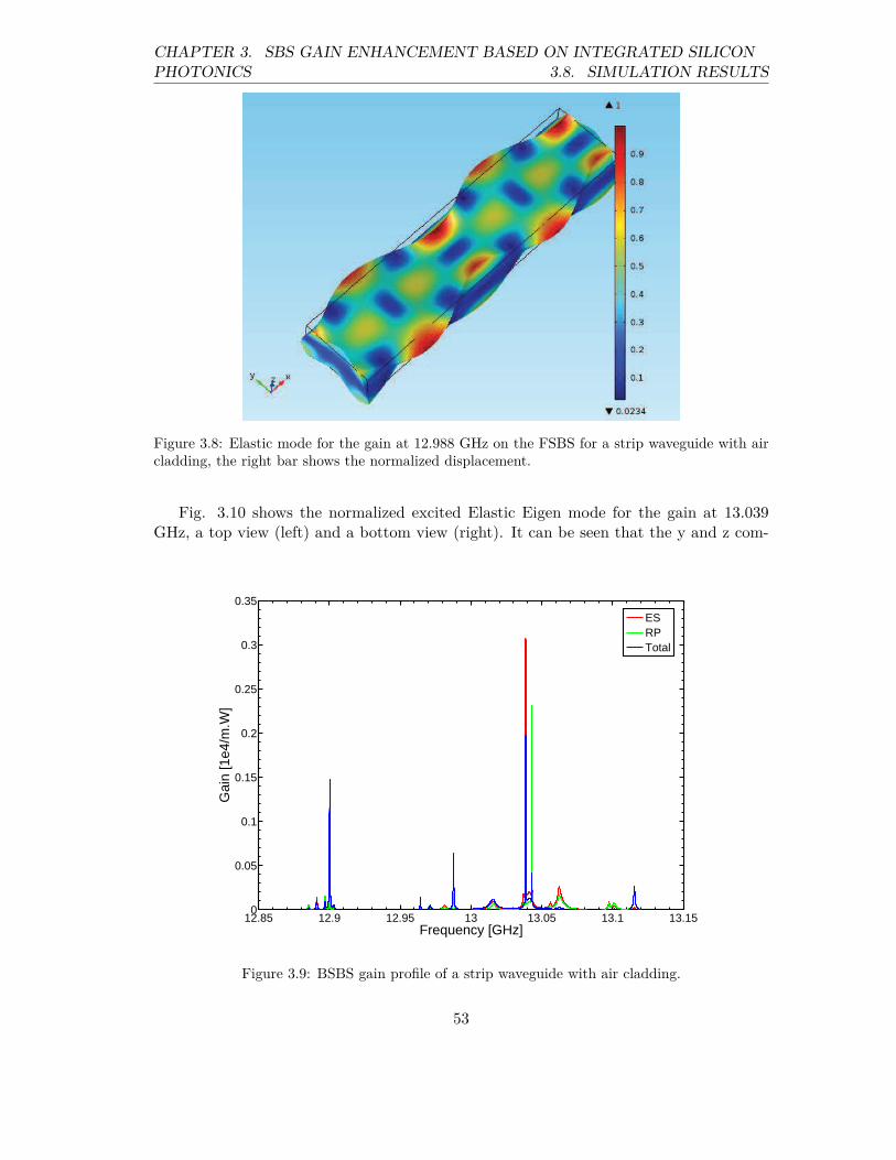
CHAPTER 3. SBS GAIN ENHANCEMENT BASED ON INTEGRATED SILICONPHOTONICS 3.8. SIMULATION RESULTS
Figure 3.8: Elastic mode for the gain at 12.988 GHz on the FSBS for a strip waveguide with aircladding, the right bar shows the normalized displacement.
Fig. 3.10 shows the normalized excited Elastic Eigen mode for the gain at 13.039GHz, a top view (left) and a bottom view (right). It can be seen that the y and z com-
12.85 12.9 12.95 13 13.05 13.1 13.150
0.05
0.1
0.15
0.2
0.25
0.3
0.35
Frequency [GHz]
Gai
n [1
e4/m
.W]
ESRPTotal
Figure 3.9: BSBS gain profile of a strip waveguide with air cladding.
53
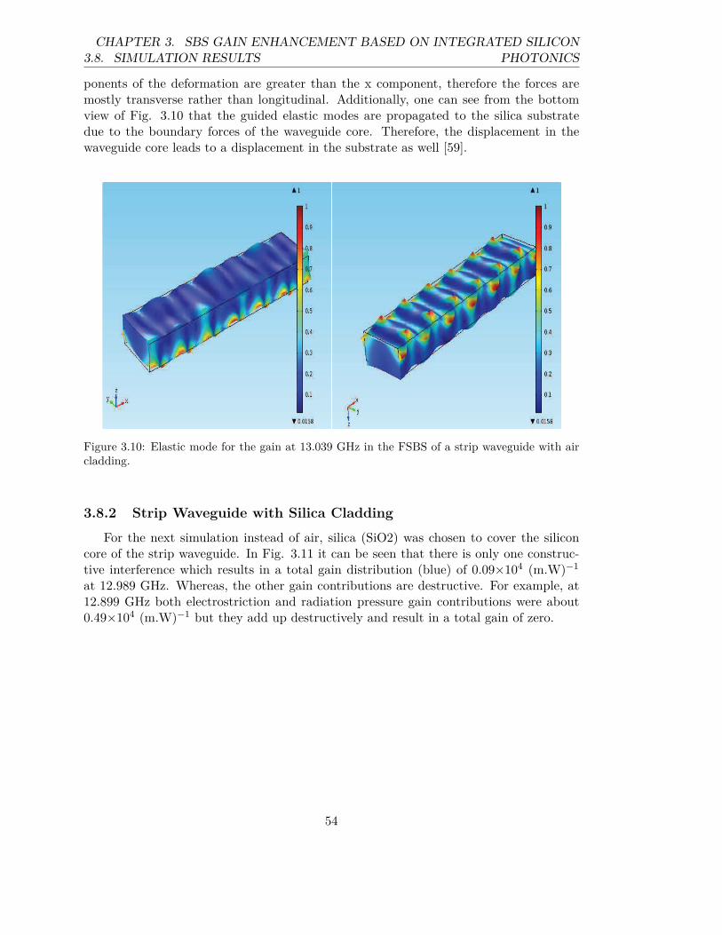
3.8. SIMULATION RESULTSCHAPTER 3. SBS GAIN ENHANCEMENT BASED ON INTEGRATED SILICON
PHOTONICS
ponents of the deformation are greater than the x component, therefore the forces aremostly transverse rather than longitudinal. Additionally, one can see from the bottomview of Fig. 3.10 that the guided elastic modes are propagated to the silica substratedue to the boundary forces of the waveguide core. Therefore, the displacement in thewaveguide core leads to a displacement in the substrate as well [59].
Figure 3.10: Elastic mode for the gain at 13.039 GHz in the FSBS of a strip waveguide with aircladding.
3.8.2 Strip Waveguide with Silica Cladding
For the next simulation instead of air, silica (SiO2) was chosen to cover the siliconcore of the strip waveguide. In Fig. 3.11 it can be seen that there is only one construc-tive interference which results in a total gain distribution (blue) of 0.09×10⁴ (m.W)−1
at 12.989 GHz. Whereas, the other gain contributions are destructive. For example, at12.899 GHz both electrostriction and radiation pressure gain contributions were about0.49×104 (m.W)−1 but they add up destructively and result in a total gain of zero.
54

CHAPTER 3. SBS GAIN ENHANCEMENT BASED ON INTEGRATED SILICONPHOTONICS 3.8. SIMULATION RESULTS
12.84 12.86 12.88 12.9 12.92 12.94 12.96 12.98 130
0.1
0.2
0.3
0.4
0.5
Frequency [GHz]
Gai
n [1
e4/m
.W]
ESRPTotal
Figure 3.11: FSBS gain profile of a strip waveguide with silica cladding.
Fig. 3.12 shows the normalized elastic deformation of the gain at 12.988 GHz forFSBS, the oscillation takes place mainly in y and z at the button side of the core, i.e.the dominant force is transverse.
Figure 3.12: Elastic mode for the gain at 12.988 GHz in FSBS of a strip waveguide with silicacladding.
55
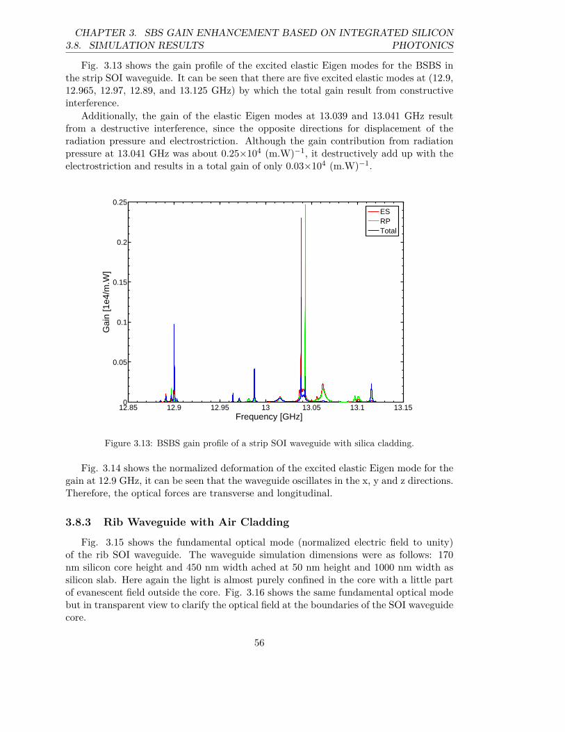
3.8. SIMULATION RESULTSCHAPTER 3. SBS GAIN ENHANCEMENT BASED ON INTEGRATED SILICON
PHOTONICS
Fig. 3.13 shows the gain profile of the excited elastic Eigen modes for the BSBS inthe strip SOI waveguide. It can be seen that there are five excited elastic modes at (12.9,12.965, 12.97, 12.89, and 13.125 GHz) by which the total gain result from constructiveinterference.
Additionally, the gain of the elastic Eigen modes at 13.039 and 13.041 GHz resultfrom a destructive interference, since the opposite directions for displacement of theradiation pressure and electrostriction. Although the gain contribution from radiationpressure at 13.041 GHz was about 0.25×10⁴ (m.W)−1, it destructively add up with theelectrostriction and results in a total gain of only 0.03×10⁴ (m.W)−1.
12.85 12.9 12.95 13 13.05 13.1 13.150
0.05
0.1
0.15
0.2
0.25
Frequency [GHz]
Gai
n [1
e4/m
.W]
ESRPTotal
Figure 3.13: BSBS gain profile of a strip SOI waveguide with silica cladding.
Fig. 3.14 shows the normalized deformation of the excited elastic Eigen mode for thegain at 12.9 GHz, it can be seen that the waveguide oscillates in the x, y and z directions.Therefore, the optical forces are transverse and longitudinal.
3.8.3 Rib Waveguide with Air Cladding
Fig. 3.15 shows the fundamental optical mode (normalized electric field to unity)of the rib SOI waveguide. The waveguide simulation dimensions were as follows: 170nm silicon core height and 450 nm width ached at 50 nm height and 1000 nm width assilicon slab. Here again the light is almost purely confined in the core with a little partof evanescent field outside the core. Fig. 3.16 shows the same fundamental optical modebut in transparent view to clarify the optical field at the boundaries of the SOI waveguidecore.
56
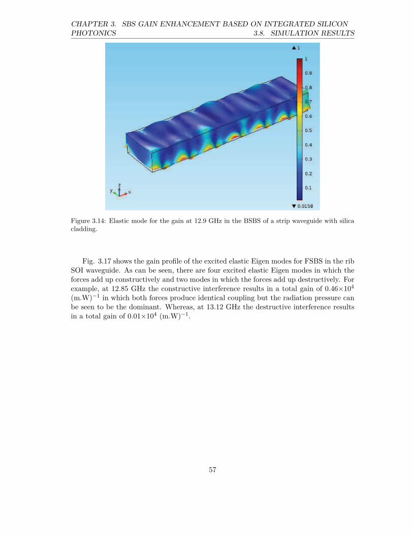
CHAPTER 3. SBS GAIN ENHANCEMENT BASED ON INTEGRATED SILICONPHOTONICS 3.8. SIMULATION RESULTS
Figure 3.14: Elastic mode for the gain at 12.9 GHz in the BSBS of a strip waveguide with silicacladding.
Fig. 3.17 shows the gain profile of the excited elastic Eigen modes for FSBS in the ribSOI waveguide. As can be seen, there are four excited elastic Eigen modes in which theforces add up constructively and two modes in which the forces add up destructively. Forexample, at 12.85 GHz the constructive interference results in a total gain of 0.46×10⁴
(m.W)−1 in which both forces produce identical coupling but the radiation pressure canbe seen to be the dominant. Whereas, at 13.12 GHz the destructive interference resultsin a total gain of 0.01×10⁴ (m.W)−1.
57
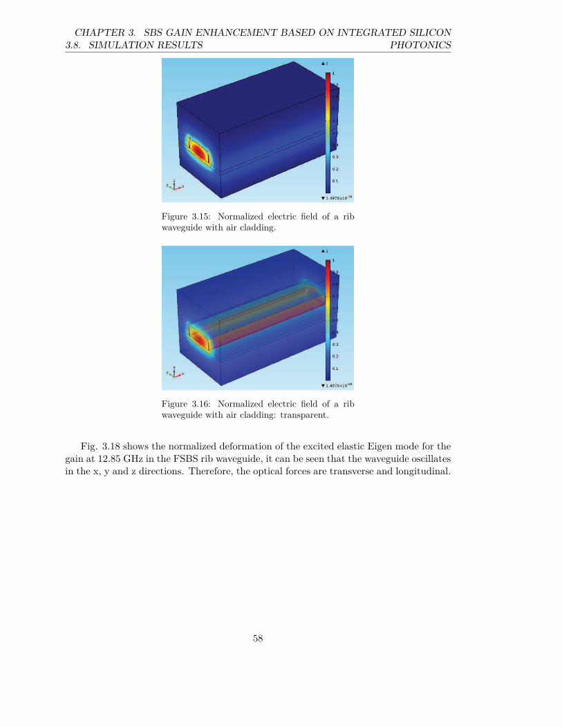
3.8. SIMULATION RESULTSCHAPTER 3. SBS GAIN ENHANCEMENT BASED ON INTEGRATED SILICON
PHOTONICS
Figure 3.15: Normalized electric field of a ribwaveguide with air cladding.
Figure 3.16: Normalized electric field of a ribwaveguide with air cladding: transparent.
Fig. 3.18 shows the normalized deformation of the excited elastic Eigen mode for thegain at 12.85 GHz in the FSBS rib waveguide, it can be seen that the waveguide oscillatesin the x, y and z directions. Therefore, the optical forces are transverse and longitudinal.
58
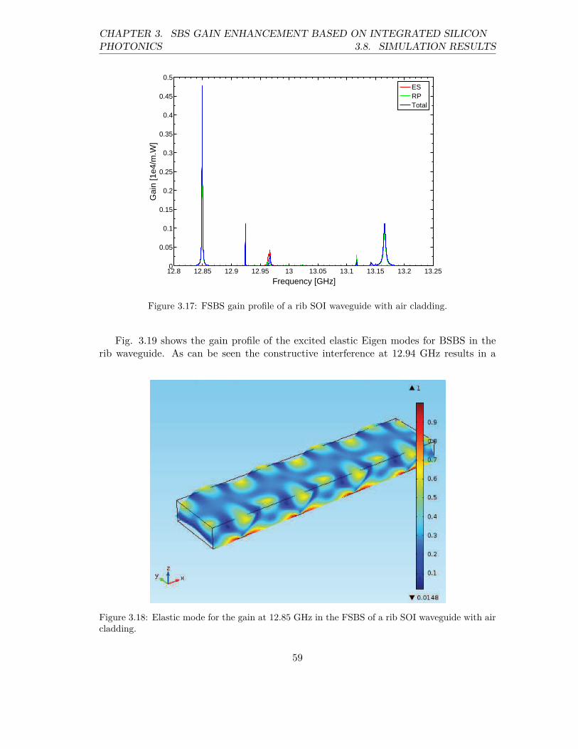
CHAPTER 3. SBS GAIN ENHANCEMENT BASED ON INTEGRATED SILICONPHOTONICS 3.8. SIMULATION RESULTS
12.8 12.85 12.9 12.95 13 13.05 13.1 13.15 13.2 13.250
0.05
0.1
0.15
0.2
0.25
0.3
0.35
0.4
0.45
0.5
Frequency [GHz]
Gai
n [1
e4/m
.W]
ESRPTotal
Figure 3.17: FSBS gain profile of a rib SOI waveguide with air cladding.
Fig. 3.19 shows the gain profile of the excited elastic Eigen modes for BSBS in therib waveguide. As can be seen the constructive interference at 12.94 GHz results in a
Figure 3.18: Elastic mode for the gain at 12.85 GHz in the FSBS of a rib SOI waveguide with aircladding.
59

3.8. SIMULATION RESULTSCHAPTER 3. SBS GAIN ENHANCEMENT BASED ON INTEGRATED SILICON
PHOTONICS
12.8 12.85 12.9 12.95 13 13.05 13.1 13.15 13.2 13.250
0.2
0.4
0.6
0.8
1
1.2
1.4
Frequency [GHz]
Gai
n [1
e4/m
.W]
ESRPTotal
12.935 12.94 12.9450
0.2
0.4
0.6
0.8
1
1.2
1.4
Frequency [GHz]
Gai
n [1
e4/m
.W]
Figure 3.19: BSBS gain profile of a rib SOI waveguide with air cladding.
significant total gain of 1.32×10⁴ (m.W)−1.The inset of Fig. 3.19 shows a magnified gain profile of the excited elastic Eigen mode
at 12.94 GHz. As can be seen the radiation results in a gain of 0.41×10⁴ (m.W)−1 andthe electrostriction results in a gain of 0.25×10⁴ (m.W)−1.
Fig. 3.20 shows the normalized deformation of the excited elastic Eigen mode forthe gain at 12.95 GHz in the BSBS rib waveguide, it can be seen that the waveguideoscillates in the x, y and z directions. Therefore, the optical forces are transverse andlongitudinal.
60
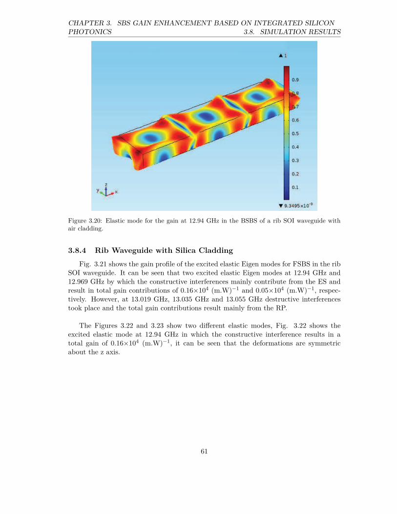
CHAPTER 3. SBS GAIN ENHANCEMENT BASED ON INTEGRATED SILICONPHOTONICS 3.8. SIMULATION RESULTS
Figure 3.20: Elastic mode for the gain at 12.94 GHz in the BSBS of a rib SOI waveguide withair cladding.
3.8.4 Rib Waveguide with Silica Cladding
Fig. 3.21 shows the gain profile of the excited elastic Eigen modes for FSBS in the ribSOI waveguide. It can be seen that two excited elastic Eigen modes at 12.94 GHz and12.969 GHz by which the constructive interferences mainly contribute from the ES andresult in total gain contributions of 0.16×10⁴ (m.W)−1 and 0.05×10⁴ (m.W)−1, respec-tively. However, at 13.019 GHz, 13.035 GHz and 13.055 GHz destructive interferencestook place and the total gain contributions result mainly from the RP.
The Figures 3.22 and 3.23 show two different elastic modes, Fig. 3.22 shows theexcited elastic mode at 12.94 GHz in which the constructive interference results in atotal gain of 0.16×10⁴ (m.W)−1, it can be seen that the deformations are symmetricabout the z axis.
61
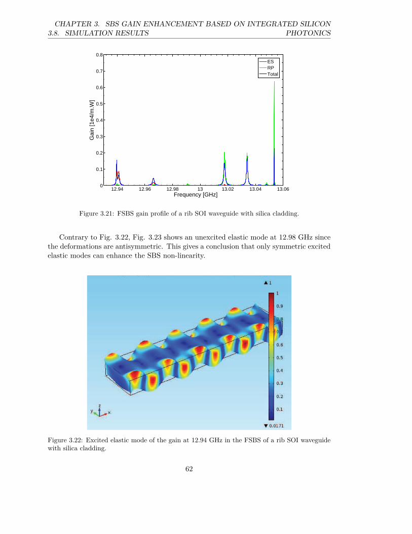
3.8. SIMULATION RESULTSCHAPTER 3. SBS GAIN ENHANCEMENT BASED ON INTEGRATED SILICON
PHOTONICS
12.94 12.96 12.98 13 13.02 13.04 13.060
0.1
0.2
0.3
0.4
0.5
0.6
0.7
0.8
Frequency [GHz]
Gai
n [1
e4/m
.W]
ESRPTotal
Figure 3.21: FSBS gain profile of a rib SOI waveguide with silica cladding.
Contrary to Fig. 3.22, Fig. 3.23 shows an unexcited elastic mode at 12.98 GHz sincethe deformations are antisymmetric. This gives a conclusion that only symmetric excitedelastic modes can enhance the SBS non-linearity.
Figure 3.22: Excited elastic mode of the gain at 12.94 GHz in the FSBS of a rib SOI waveguidewith silica cladding.
62
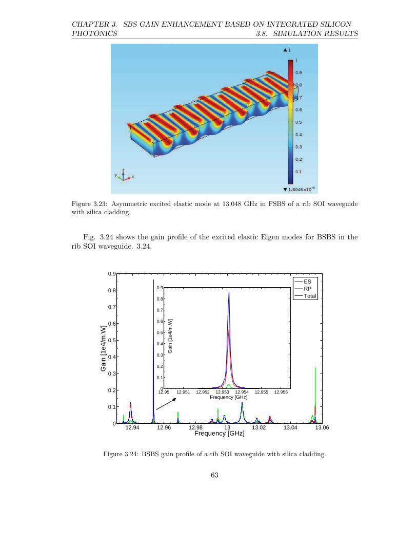
CHAPTER 3. SBS GAIN ENHANCEMENT BASED ON INTEGRATED SILICONPHOTONICS 3.8. SIMULATION RESULTS
Figure 3.23: Asymmetric excited elastic mode at 13.048 GHz in FSBS of a rib SOI waveguidewith silica cladding.
Fig. 3.24 shows the gain profile of the excited elastic Eigen modes for BSBS in therib SOI waveguide. 3.24.
12.94 12.96 12.98 13 13.02 13.04 13.060
0.1
0.2
0.3
0.4
0.5
0.6
0.7
0.8
0.9
Frequency [GHz]
Gai
n [1
e4/m
.W]
ESRPTotal
12.95 12.951 12.952 12.953 12.954 12.955 12.9560
0.1
0.2
0.3
0.4
0.5
0.6
0.7
0.8
0.9
Frequency [GHz]
Gai
n [1
e4/m
.W]
Figure 3.24: BSBS gain profile of a rib SOI waveguide with silica cladding.
63
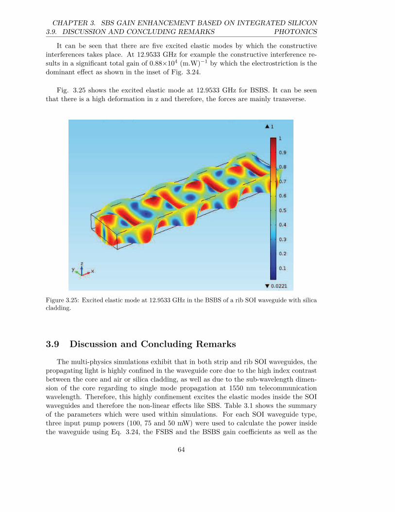
3.9. DISCUSSION AND CONCLUDING REMARKSCHAPTER 3. SBS GAIN ENHANCEMENT BASED ON INTEGRATED SILICON
PHOTONICS
It can be seen that there are five excited elastic modes by which the constructiveinterferences takes place. At 12.9533 GHz for example the constructive interference re-sults in a significant total gain of 0.88×10⁴ (m.W)−1 by which the electrostriction is thedominant effect as shown in the inset of Fig. 3.24.
Fig. 3.25 shows the excited elastic mode at 12.9533 GHz for BSBS. It can be seenthat there is a high deformation in z and therefore, the forces are mainly transverse.
Figure 3.25: Excited elastic mode at 12.9533 GHz in the BSBS of a rib SOI waveguide with silicacladding.
3.9 Discussion and Concluding Remarks
The multi-physics simulations exhibit that in both strip and rib SOI waveguides, thepropagating light is highly confined in the waveguide core due to the high index contrastbetween the core and air or silica cladding, as well as due to the sub-wavelength dimen-sion of the core regarding to single mode propagation at 1550 nm telecommunicationwavelength. Therefore, this highly confinement excites the elastic modes inside the SOIwaveguides and therefore the non-linear effects like SBS. Table 3.1 shows the summaryof the parameters which were used within simulations. For each SOI waveguide type,three input pump powers (100, 75 and 50 mW) were used to calculate the power insidethe waveguide using Eq. 3.24, the FSBS and the BSBS gain coefficients as well as the
64
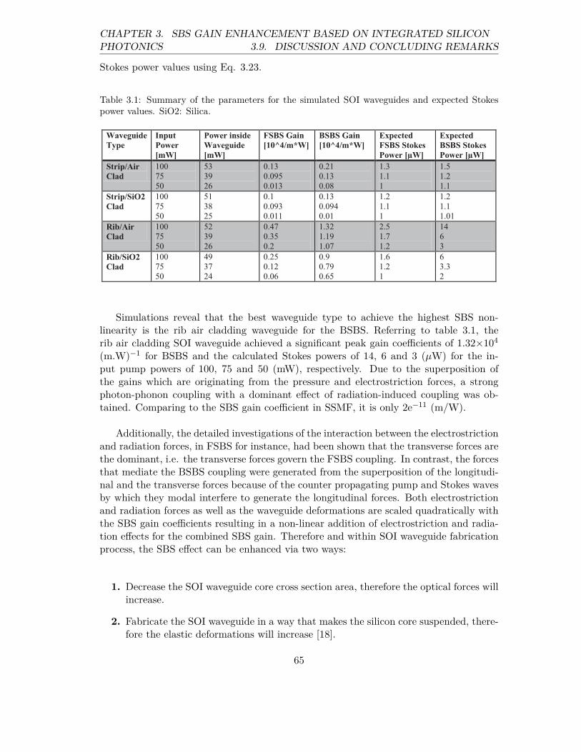
CHAPTER 3. SBS GAIN ENHANCEMENT BASED ON INTEGRATED SILICONPHOTONICS 3.9. DISCUSSION AND CONCLUDING REMARKS
Stokes power values using Eq. 3.23.
Table 3.1: Summary of the parameters for the simulated SOI waveguides and expected Stokespower values. SiO2: Silica.
Waveguide
Type
Input
Power
[mW]
Power inside
Waveguide
[mW]
FSBS Gain
[10^4/m*W]
BSBS Gain
[10^4/m*W]
Expected
FSBS Stokes
Power [µW]
Expected
BSBS Stokes
Power [µW]
Strip/Air
Clad
100
75
50
53
39
26
0.13
0.095
0.013
0.21
0.13
0.08
1.3
1.1
1
1.5
1.2
1.1
Strip/SiO2
Clad
100
75
50
51
38
25
0.1
0.093
0.011
0.13
0.094
0.01
1.2
1.1
1
1.2
1.1
1.01
Rib/Air
Clad
100
75
50
52
39
26
0.47
0.35
0.2
1.32
1.19
1.07
2.5
1.7
1.2
14
6
3
Rib/SiO2
Clad
100
75
50
49
37
24
0.25
0.12
0.06
0.9
0.79
0.65
1.6
1.2
1
6
3.3
2
Simulations reveal that the best waveguide type to achieve the highest SBS non-linearity is the rib air cladding waveguide for the BSBS. Referring to table 3.1, therib air cladding SOI waveguide achieved a significant peak gain coefficients of 1.32×10⁴
(m.W)−1 for BSBS and the calculated Stokes powers of 14, 6 and 3 (µW) for the in-put pump powers of 100, 75 and 50 (mW), respectively. Due to the superposition ofthe gains which are originating from the pressure and electrostriction forces, a strongphoton-phonon coupling with a dominant effect of radiation-induced coupling was ob-tained. Comparing to the SBS gain coefficient in SSMF, it is only 2e−11 (m/W).
Additionally, the detailed investigations of the interaction between the electrostrictionand radiation forces, in FSBS for instance, had been shown that the transverse forces arethe dominant, i.e. the transverse forces govern the FSBS coupling. In contrast, the forcesthat mediate the BSBS coupling were generated from the superposition of the longitudi-nal and the transverse forces because of the counter propagating pump and Stokes wavesby which they modal interfere to generate the longitudinal forces. Both electrostrictionand radiation forces as well as the waveguide deformations are scaled quadratically withthe SBS gain coefficients resulting in a non-linear addition of electrostriction and radia-tion effects for the combined SBS gain. Therefore and within SOI waveguide fabricationprocess, the SBS effect can be enhanced via two ways:
1. Decrease the SOI waveguide core cross section area, therefore the optical forces willincrease.
2. Fabricate the SOI waveguide in a way that makes the silicon core suspended, there-fore the elastic deformations will increase [18].
65
3.10. SUGGESTED EXPERIMENTAL SETUPCHAPTER 3. SBS GAIN ENHANCEMENT BASED ON INTEGRATED SILICON
PHOTONICS
In the modes where the electrostriction forces are the dominant and referring to theelastic modes oscillations, it can be seen that transverse forces have both inward andoutward deformation directions. This can be understood from the different signs of thephoto elastic coefficients in the electrostrictive tensor. Hence, the main diagonal coeffi-cients have the minus sign while the other coefficients have the plus sign.
According to Figures 3.21 and 3.23 it can be seen that only symmetric waveguideoscillations enhance the SBS non-linearity. The direct interference between the opti-cal forces can enhance or suppress the SBS process, since the Transverse Electric (TE)like mode results in symmetric force distributions for both electrostriction and radiation.Therefore, only phonon modes with even displacement with respect to the SOI waveguidecore can achieve the effective SBS coupling.
Additionally, if the TPA effect limitation is considered and referring to the simulatedpower values inside the waveguide in table 3.1, it can be noticed that only 50 mw inputpower is possible to achieve the SBS non-linear effect, otherwise the TPA non-linear ef-fect could take place. Since for (50 mW) input pump power, the calculated power insidethe waveguide is below the TPA threshold, i.e. 30 (mW), as mentioned earlier. Referringto Eq. 3.24 by which the power inside the waveguide was calculated and the effectiverefractive index was simulated, the power loss between the input and the power inside thewaveguide was due to the coupling losses which are included in the simulated effectiverefractive index values. In principle, one can use the fiber laser or Distributed Feed Back(DFB) lasers as a pump source of 5 mW output power with several amplifiers to reachthe optimum input power of 50 (mW). Each of the fiber laser and the DFB lasers has alinewidth smaller than the SBS linewdth, therefore the expected Stokes linewidth wouldbe about the natural SBS gain linewidth relating to the convolution of the SBS gain andthe pump wave.
3.10 Suggested Experimental Setup
The suggested experimental setup to measure the SBS gain using the SOI waveguideis shown in Fig. 3.26. The blue color refers to the setup equipments that could be usedto achieve FSBS measurement while the green refers to the setup that could be used toachieve the BSBS measurement.
An optical signal would be modulated using the intensity modulator (IM) and a sweep(fmod) RF signal would be used to scan the achieved gain profile of the SOI waveguideafterwords. The bias voltage (BV) would be used to suppress the carrier of the IM andthe tuneable filter (TOF) would suppress the unwanted sideband and the remaining car-rier of the modulator. The selected sideband out of the TF would be amplified via theErbium Doped Fiber Amplifier (EDFA2) to be coupled with the amplified pump wavevia 90/10 coupler. A fiber or DFB lasers could be used as pump source. EDFA1 outputshould be set for 50 mW in order to get rid of the TPA effect. Both the pump wave(blue) and the scan signal would be launched to the SOI waveguide to achieve FSBS,
66
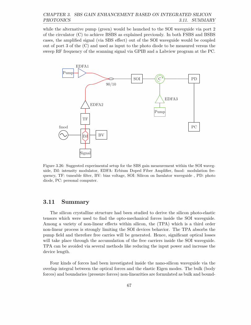
CHAPTER 3. SBS GAIN ENHANCEMENT BASED ON INTEGRATED SILICONPHOTONICS 3.11. SUMMARY
while the alternative pump (green) would be launched to the SOI waveguide via port 2of the circulator (C) to achieve BSBS as explained previously. In both FSBS and BSBScases, the amplified signal (via SBS effect) out of the SOI waveguide would be coupledout of port 3 of the (C) and used as input to the photo diode to be measured versus thesweep RF frequency of the scanning signal via GPIB and a Labview program at the PC.
Pump
90/10
EDFA1
EDFA2
TF
IM
fmod
Signal
BV
PC
PDSOI C
EDFA3
Pump
Figure 3.26: Suggested experimental setup for the SBS gain measurement within the SOI waveg-uide, IM: intensity modulator, EDFA: Erbium Doped Fiber Amplifier, fmod: modulation fre-quency, TF: tuneable filter, BV: bias voltage, SOI: Silicon on Insulator waveguide , PD: photodiode, PC: personal computer.
3.11 Summary
The silicon crystalline structure had been studied to derive the silicon photo-elastictensors which were used to find the opto-mechanical forces inside the SOI waveguide.Among a variety of non-linear effects within silicon, the (TPA) which is a third ordernon-linear process is strongly limiting the SOI devices behavior. The TPA absorbs thepump field and therefore free carries will be generated. Hence, significant optical losseswill take place through the accumulation of the free carriers inside the SOI waveguide.TPA can be avoided via several methods like reducing the input power and increase thedevice length.
Four kinds of forces had been investigated inside the nano-silicon waveguide via theoverlap integral between the optical forces and the elastic Eigen modes. The bulk (bodyforces) and boundaries (pressure forces) non-linearities are formulated as bulk and bound-
67

3.11. SUMMARYCHAPTER 3. SBS GAIN ENHANCEMENT BASED ON INTEGRATED SILICON
PHOTONICS
ary integrals over the waveguide cross section and boundaries, respectively. Both bodyand pressure electrostriction forces had been derived from the photo-elastic tensor. Theradiation body and pressure forces had been derived from the Maxwells stress tensor.
The Brillouin gain had been calculated from the overlap integral between all forcesand the elastic deformation which is caused by the forces. The integration is taken overthe waveguide cross section for body forces, while for pressure forces the integration istaken over the boundaries.
Two kinds of waveguides are investigated: strip and rib waveguides. For each kind,two cases are studied: air and silica cladding. The FSBS and BSBS gain within thewave guide had been calculated. It is shown that an unprecedented high SBS gain witha large magnitude can be found in many elastic Eigen-modes. A constructive interfer-ence between the forces could be found mainly with symmetric deformation of the SOIwaveguide. The rib air cladding waveguide was achieved the highest BSBS non-linearitywith a significant peak gain of 1.32×10⁴ (m.W)−1 which is order of magnitudes higherthan the optical fibers peak gain coefficient.
In table 3.1, three pump powers (100, 75, and 50 mW) were simulated to find theappropriate pump power for the waveguide. It is found that with 50 (mW) pump power,the power inside the waveguide is below the TPA threshold which is 30 (mW). Therefore,the recommended maximum pump power within the suggested experimental setup was50 mW.
68
Chapter 4
Extraction of High Quality Single LaserLines
4.1 Introduction
Since the high interest in coherent detection systems as a local oscillator for opticalcommunications as well as high resolution spectroscopy, wavelength-division multiplexing(WDM) systems and multilevel modulation formats, great efforts had been payed towardthe development of stable, widely wavelength-tuneable and narrow linewidth single linelasers [60, 61, 62, 63]. Highly stable and narrow linewidth lasers are very important fordigital coherent detection systems, since they are used as a technique for the enhance-ment of the capacity and spectral quality of the next-generation fiber-optical networks[64]. For optical sensors such high quality lasers, mainly stable single line lasers, arenecessary as well.
Many methods had been demonstrated to achieve the desired requirements of the sin-gle line laser, such as widely tuneable, narrow linewidth and stable lasers for the abovementioned applications. For example, less than 5 MHz laser linewidth over 40 nm tuningrange was reported using a distributed Bragg reflector (DBR) laser [65]. Additionally,in [66] a single-longitudinal mode laser with a linewidth of less than 20 kHz using along-cavity, narrow-bandwidth SBS as filter and multi-frequency selection mechanismsimultaneously had been presented. In [67] a linewidth of less than 5 kHz and a stabilityof 62.2 MHz for a single longitudinal mode laser is reported using spectral overlappingof two uniform fiber Bragg gratings (FBG). On the other hand, a method to reducethe linewidth of commercially available distributed feedback (DFB) laser diodes down to1.8 kHz with an electro-optical feed-forward loop was reported [68]. Since the SBS gainbandwidth can be reduced via several amplification stages [69], a linewidth below 1 kHzof a single frequency and continuous wave Brillouin fiber-ring laser was achieved by uti-lizing an unbalanced Mach-Zehnder interferometer as a coupling device [70]. Regardingthe laser tuneability, a conventional DFB laser diode has a tuneability range of 2-6 nm.
69
4.1. INTRODUCTIONCHAPTER 4. EXTRACTION OF HIGH QUALITY SINGLE LASER LINES
However, in [68] a tuneability range of 40 nm was reported for a DFB laser.
In principle, all the previous attempts for enhancing the lasers quality are limitedeither in the minimum linewidth or tuneability range, or both. Therefore, in this chap-ter a simple method to extract one spectral laser line out of a frequency comb which isgenerated by a mode-locked fiber laser (MLFL) will be demonstrated and experimentallyimplemented. The frequency comb has unique features such as broad bandwidth i.e.thousands of spectral lines with equidistant frequency spacing (25 MHz up to 10 GHzdepending on the resonator length [76]) and a highly stable amplitude. Additionally,according to [71, 72] some frequency combs have a bandwidth of about 100 nm and thelinewidth of each spectral mode could reach down to sub-millihertz.
In order to extract one spectral line out of thousands of lines, a narrow band opticalfilter is required. Thus, if the repetition rate is in the range of 100 MHz, an optical filterwith a bandwidth less than 100 MHz is needed. Therefore, conventional optical filters arenot sufficient such as a wave shaper optical filter which has a minimum bandwidth of 10GHz or a coated thin film band bass filter which has a bandwidth in the GHz range. In[73] for example, a 325 MHz bandpass filter is reported via Fiber Bragg Gratings (FBG).Narrow FBG cannot be tuned very far and conventional FBGs are too broad. However,in [74] a Fabry-Perot filter of 250 MHz bandwidth with several filter modes as well as arepetitive structure was reported.
Thus, here the non-linear effect of polarization pulling assisted SBS (PPA-SBS) hadbeen utilized as a filter and amplifier [26]. Such a filter offers a narrow bandwidth in theorder of 10-30 MHz within standard single mode fibers (SSMF). Therefore, the band-width of PPA-SBS is less than the frequency difference between any two neighboringspectral lines of the frequency comb. Hence, any specific spectral line can be discrimi-nated. In principle, the idea behind the extraction of the desired spectral comb line viaPPA-SBS is the suppression of the unwanted spectral lines via the careful polarizationsetting of the pump wave (which is used to generate the SBS effect) and the pre-filtered(to provide sufficient signal to noise ratio for the next step) comb lines by a polarizationcontroller. Therefore, the state of polarization of the desired and amplified spectral combline via SBS is perpendicular to the state of polarization of the unwanted comb lines.Additionally, the linewidth determination of the extracted spectral line is very important.Therefore, several techniques will be presented to determine the linewidth of the spectralline.
This chapter is organized as follows: optical frequency comb operation principlesand generation are explained. The polarization pulling assisted SBS is introduced andthe previously derived SBS differential equations are modified depending on the stateof polarization of both pump and Stokes waves. Several laser linewidth measurementtechniques are presented. The experimental setup and results for the extraction of thelaser, linewidth measurement, tuneability and stabilization are presented as well. Finally,a discussion, concluding remarks and a summery are given.
70

CHAPTER 4. EXTRACTION OF HIGH QUALITY SINGLE LASER LINES4.2. OPTICAL FREQUENCY COMBS
4.2 Optical Frequency Combs
In the late 1970s the optical frequency comb was developed through a picosecond laser[75]. There are many different mechanisms to generate optical frequency combs including:amplitude modulation of a continuous wave laser, four wave mixing, micro-ring resonatoror a mode locking inside a lasers cavity [76]. The most popular and famous mechanism forachieving a frequency comb is a mode locked laser (MLL). In the frequency-domain thefrequency comb consists of thousands of equidistant narrow spectral lines over a broadspectral range each spectral line is known as a mode. If all these frequencies (modes)are locked in phase, i.e. fixed phase relationship between all of the lasing longitudinalmodes, this corresponds to a sequence of pulses in the time domain. Fig. 4.1 shows therepresentation of a pulse train composition by adding three waves with different frequen-cies (modes). The vertical black line refers to the time points where all waves are equalin phase.
0 2 4 6 8 10 12−0.5
0
0.5
0 2 4 6 8 10 12−1
0
1
0 2 4 6 8 10 12−2
0
2
Am
plitu
de [a
.u]
0 2 4 6 8 10 12
−5
0
5
Time [a.u.]
Figure 4.1: Pulse train composition (solid blue) by superposition of three different frequencywaves.
Generally, the laser requires a cavity consisting of two mirrors with different perme-
71
4.2. OPTICAL FREQUENCY COMBSCHAPTER 4. EXTRACTION OF HIGH QUALITY SINGLE LASER LINES
ability by which the laser light can resonate (radiate) and pass through a gain medium.The gain medium such as an erbium-doped fiber will compensate for losses during thelight propagation inside the cavity. Laser diodes are mainly used for the pumping ofMLL. Hence, the laser diode provides energy to the gain medium, whereas the circulat-ing pulse reproduces energy in a uniform time period. The term mode locking refers tothe method by which ultra-short laser pulses can be obtained. For mode locking, thelaser cavity needs to contain either an active element such as an optical modulator ora non-linear passive element such as a saturable absorber. Therefore, the formation ofultra-short pulses will circulate inside the laser cavity. Every time the pulse hits theoutput coupler mirror, a part of the pulse will be emitted and therefore a pulse train willbe generated.
The different frequency lines are separated by the repetition rate which is the inverseof the round trip time of the laser resonator. Whereas, the pulse duration is inverselyrelated to the number of the involved modes times the frequency spacing between them,i.e. more involved modes result in a shorter pulse duration.
Frequency combs are commonly used in metrology [77]. In the field of ultrafast spec-troscopy the interest is to achieve extremely short time domain bursts of the electric field,which requires a large spectral bandwidth. In contrast, in the field of precision measure-ments the interest is to have lasers with a very narrow spectral linewidth. Therefore,both requirements can be satisfied simultaneously by utilizing a MLL frequency comb.Frequency combs can also be used for atomic clocks and Lidar (inspecting technologyby which a distance can be measured by illuminating a target with a laser light) or thesynthesization of arbitrary optical waveforms by modulating the phase and amplitudeof individual lines [78, 79, 80]. Moreover, the extraction of spectral lines out of the fre-quency comb is very important. For example, they can be used to generate high qualitysingle line lasers [24], as well as high quality microwaves with phase noise much lower thanachievable by conventional microwave oscillators as will be shown in the next chapter [25].
To understand how the mode-locked laser is working, a simulation model had beenmade for 100 modes without phase coherence between the modes, the results are shownin Fig. 4.2. In principle, the simulated model adds up cavity electrical field modes. Thecavity and simulation parameters were set as follows:
The noise factor was either 0 (phase locking) or >> 0 (large phase noise), the cavitylength was l = 1.5 m, and the free spectral range of the cavity was FSR = c0/(2×l).The total electric field E = Em cos (2πft+ ∆ν), where f is a frequency goes from funda-mental to higher laser frequencies with a step of the free spectral range, ∆ν is the phaseand t is the time from 0 to 50 ns.
72
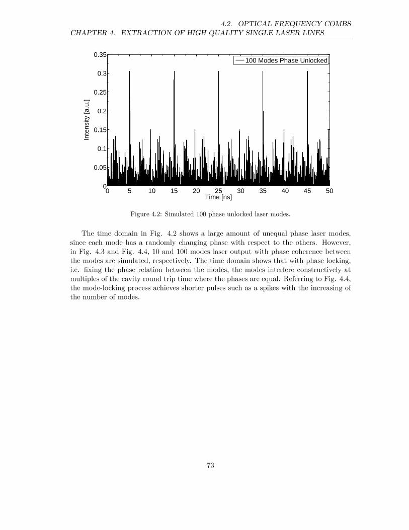
CHAPTER 4. EXTRACTION OF HIGH QUALITY SINGLE LASER LINES4.2. OPTICAL FREQUENCY COMBS
0 5 10 15 20 25 30 35 40 45 500
0.05
0.1
0.15
0.2
0.25
0.3
0.35
Time [ns]
Inte
nsity
[a.u
.]
100 Modes Phase Unlocked
Figure 4.2: Simulated 100 phase unlocked laser modes.
The time domain in Fig. 4.2 shows a large amount of unequal phase laser modes,since each mode has a randomly changing phase with respect to the others. However,in Fig. 4.3 and Fig. 4.4, 10 and 100 modes laser output with phase coherence betweenthe modes are simulated, respectively. The time domain shows that with phase locking,i.e. fixing the phase relation between the modes, the modes interfere constructively atmultiples of the cavity round trip time where the phases are equal. Referring to Fig. 4.4,the mode-locking process achieves shorter pulses such as a spikes with the increasing ofthe number of modes.
73
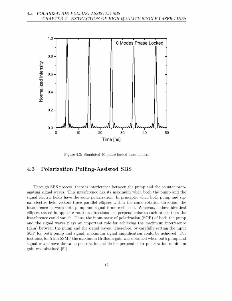
4.3. POLARIZATION PULLING-ASSISTED SBSCHAPTER 4. EXTRACTION OF HIGH QUALITY SINGLE LASER LINES
0 10 20 30 40 500.0
0.2
0.4
0.6
0.8
1.0N
orm
aliz
ed In
tens
ity
Time [ns]
10 Modes Phase Locked
Figure 4.3: Simulated 10 phase locked laser modes.
4.3 Polarization Pulling-Assisted SBS
Through SBS process, there is interference between the pump and the counter prop-agating signal waves. This interference has its maximum when both the pump and thesignal electric fields have the same polarization. In principle, when both pump and sig-nal electric field vectors trace parallel ellipses within the same rotation direction, theinterference between both pump and signal is more efficient. Whereas, if these identicalellipses traced in opposite rotation directions i.e. perpendicular to each other, then theinterference could vanish. Thus, the input state of polarization (SOP) of both the pumpand the signal waves plays an important role for achieving the maximum interference(gain) between the pump and the signal waves. Therefore, by carefully setting the inputSOP for both pump and signal, maximum signal amplification could be achieved. Forinstance, for 5 km SSMF the maximum Brillouin gain was obtained when both pump andsignal waves have the same polarization, while for perpendicular polarization minimumgain was obtained [81].
74

CHAPTER 4. EXTRACTION OF HIGH QUALITY SINGLE LASER LINES4.3. POLARIZATION PULLING-ASSISTED SBS
0 10 20 30 40 500.0
0.2
0.4
0.6
0.8
1.0
Nor
mal
ized
Inte
nsity
Time [ns]
100 Modes Phase locked
Figure 4.4: Simulated 100 phase locked laser modes.
As mentioned earlier, in order to select one spectral line of the frequency comb, anarrow bandwidth optical filter is required where its bandwidth should be less than thefrequency difference between each neighboring spectral lines. Hence, conventional opticalfilters are not sufficient and therefore the PPA-SBS will be utilized as can be seen later.
According to [82], to describe the SOP of an optical signal the Stokes representationcan be used as [S = S0, S1, S2, S3], where (S) is the SOP of the incident light and(S0, S1, S2, S3) are the SOP of the light emerging from the four quadrants of the half-shade system, see [82] for more details. Therefore, if two coherent optical co-propagatingsignals with polarizations (Sa, Sb) are mixed at a photomixer, the mixing efficiency canbe written as [83]:
ψ(=⇒) =1
2(SaSb) =
1
2(1 + S1aS1b + S2aS2b + S3aS3b) (4.1)
where the components S1, S2, S3 are considered to be normalized to unit intensity S0 = 1.Additionally, no depolarization of the forward pump wave is considered, i.e., (s2
1+s22+s2
3 =1).
In principle, the mixing efficiency can be considered as a punishment against polar-ization mismatch at a coherent mixer. Hence, for co-propagating (=⇒) optical signals
75
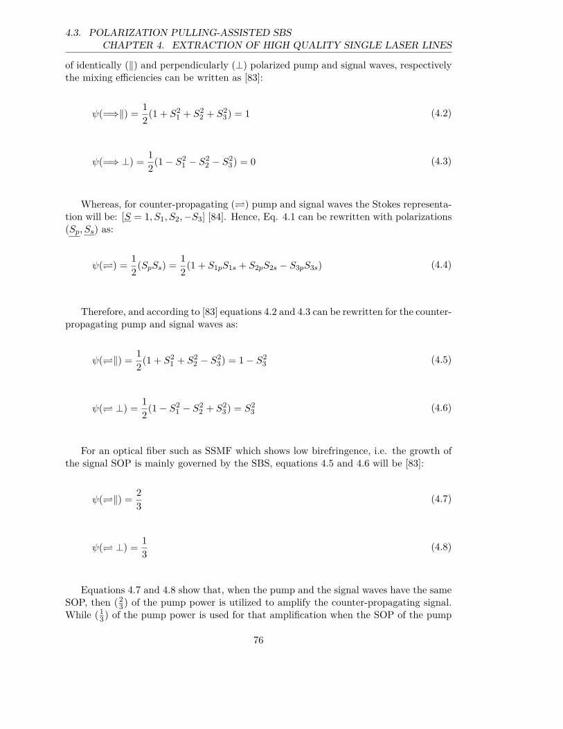
4.3. POLARIZATION PULLING-ASSISTED SBSCHAPTER 4. EXTRACTION OF HIGH QUALITY SINGLE LASER LINES
of identically (‖) and perpendicularly (⊥) polarized pump and signal waves, respectivelythe mixing efficiencies can be written as [83]:
ψ(=⇒‖) =1
2(1 + S2
1 + S22 + S2
3) = 1 (4.2)
ψ(=⇒ ⊥) =1
2(1 − S2
1 − S22 − S2
3) = 0 (4.3)
Whereas, for counter-propagating () pump and signal waves the Stokes representa-tion will be: [S = 1, S1, S2,−S3] [84]. Hence, Eq. 4.1 can be rewritten with polarizations(Sp, Ss) as:
ψ() =1
2(SpSs) =
1
2(1 + S1pS1s + S2pS2s − S3pS3s) (4.4)
Therefore, and according to [83] equations 4.2 and 4.3 can be rewritten for the counter-propagating pump and signal waves as:
ψ(‖) =1
2(1 + S2
1 + S22 − S2
3) = 1 − S23 (4.5)
ψ( ⊥) =1
2(1 − S2
1 − S22 + S2
3) = S23 (4.6)
For an optical fiber such as SSMF which shows low birefringence, i.e. the growth ofthe signal SOP is mainly governed by the SBS, equations 4.5 and 4.6 will be [83]:
ψ(‖) =2
3(4.7)
ψ( ⊥) =1
3(4.8)
Equations 4.7 and 4.8 show that, when the pump and the signal waves have the sameSOP, then (2
3) of the pump power is utilized to amplify the counter-propagating signal.While (1
3) of the pump power is used for that amplification when the SOP of the pump
76
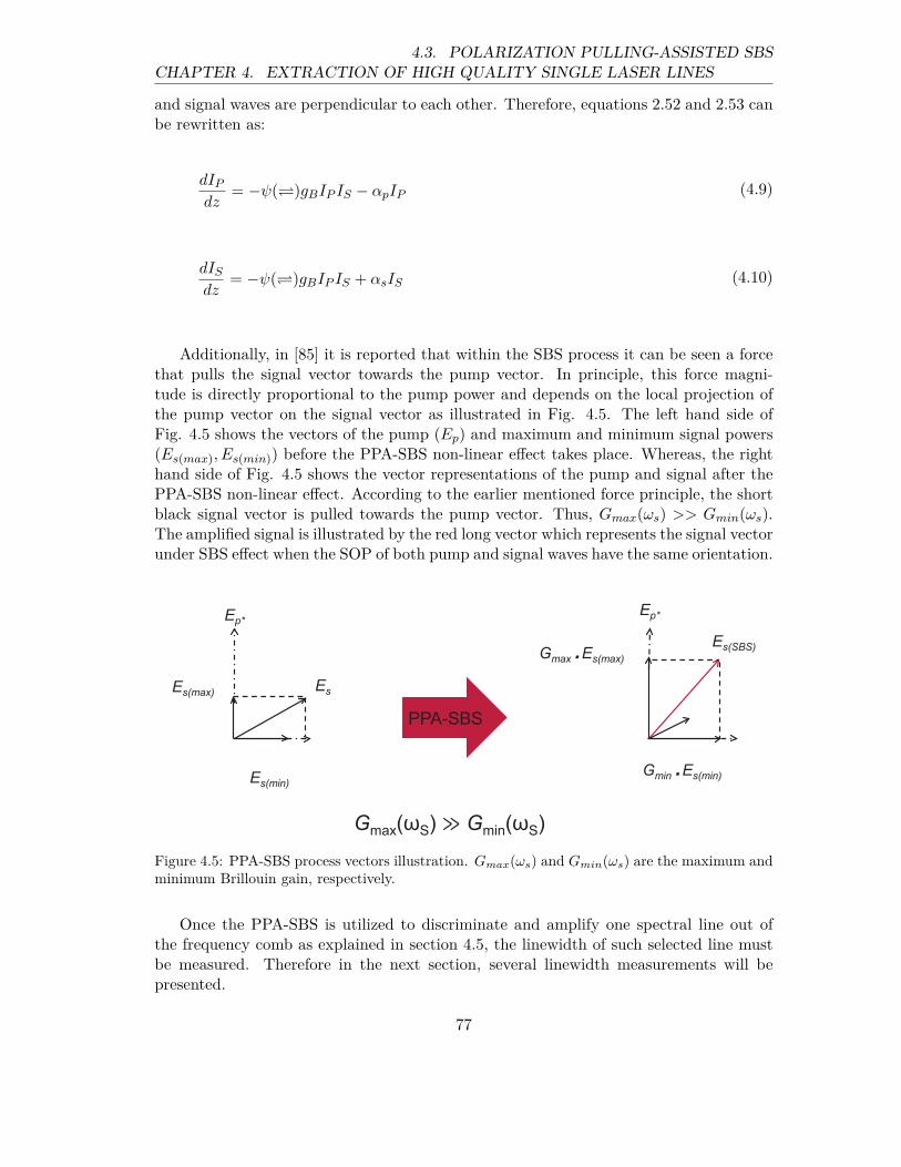
CHAPTER 4. EXTRACTION OF HIGH QUALITY SINGLE LASER LINES4.3. POLARIZATION PULLING-ASSISTED SBS
and signal waves are perpendicular to each other. Therefore, equations 2.52 and 2.53 canbe rewritten as:
dIP
dz= −ψ()gBIP IS − αpIP (4.9)
dIS
dz= −ψ()gBIP IS + αsIS (4.10)
Additionally, in [85] it is reported that within the SBS process it can be seen a forcethat pulls the signal vector towards the pump vector. In principle, this force magni-tude is directly proportional to the pump power and depends on the local projection ofthe pump vector on the signal vector as illustrated in Fig. 4.5. The left hand side ofFig. 4.5 shows the vectors of the pump (Ep) and maximum and minimum signal powers(Es(max), Es(min)) before the PPA-SBS non-linear effect takes place. Whereas, the righthand side of Fig. 4.5 shows the vector representations of the pump and signal after thePPA-SBS non-linear effect. According to the earlier mentioned force principle, the shortblack signal vector is pulled towards the pump vector. Thus, Gmax(ωs) >> Gmin(ωs).The amplified signal is illustrated by the red long vector which represents the signal vectorunder SBS effect when the SOP of both pump and signal waves have the same orientation.
PPA-SBS
Ep*Ep*
Es(max) Es
Gmax .Es(max)
Gmin .Es(min)
Es(SBS)
Es(min)
Gmax( S) Gmin( S)
Figure 4.5: PPA-SBS process vectors illustration. Gmax(ωs) and Gmin(ωs) are the maximum andminimum Brillouin gain, respectively.
Once the PPA-SBS is utilized to discriminate and amplify one spectral line out ofthe frequency comb as explained in section 4.5, the linewidth of such selected line mustbe measured. Therefore in the next section, several linewidth measurements will bepresented.
77
4.4. LASER LINEWIDTH MEASUREMENT TECHNIQUESCHAPTER 4. EXTRACTION OF HIGH QUALITY SINGLE LASER LINES
4.4 Laser Linewidth Measurement Techniques
Many applications require a full characterization of the laser parameters. For exam-ple, a laser linewidth measurement gives high potential for atomic physics, metrology andtelecommunications applications, to name a few [86, 87, 88]. Additionally, in communica-tions the proper narrow linewidth lasers and the high transmission rates demands coulddevelop the coherent communications to the next step [89]. Since the linewidth is directlyrelated to the achieved signal to noise ratio (SNR), these applications depend directly onthe linewidth of the used lasers. Thus linewidths in and below the kHz are highly recom-mended for several applications and research fields. Many techniques are demonstratedto measure the laser linewidth, mainly based on the interference of two optical fields at aproper photo diode (PD) or converting frequency fluctuations into intensity fluctuationsusing a Mach-Zehnder interferometer. Here they are explained briefly.
4.4.1 Heterodyning with a Local Oscillator
In principle, the interference between two optical fields at a proper PD (non-linearelement) results in a beat note frequency centered at the frequency difference betweenthe interfered optical waves. The resulting linewidth is a convolution of both waveslinewidths. The photo-current out of the PD, is analyzed at an electrical spectrum an-alyzer (ESA). Hence, the resultant beat note characteristics can be investigated in theelectrical domain.The two optical fields are the laser under test (LUT ) which has unknown spectral char-acteristics and the local oscillator laser as a reference. The response at the ESA containsthe direct detection part between the PD and the ESA and the heterodyne spectrumpart. The relation that governs the power spectrum out of the PD is [90]:
Si(f) ∼= R2
Sd(f)︸ ︷︷ ︸direct detection
+ 2[SLO(ν) ⊗ SLUT (−ν)]︸ ︷︷ ︸heterodyne spectrum
(4.11)
where R is the PD responsivity, Sd(f) is the ordinary direct detection spectrum at theESA, [SLO(ν)⊗SLUT (−ν)] is the heterodyne mixing part which is a convolution betweenthe local oscillator and the LUT signal. The time-varying multiplication between thelocal oscillator and the LUT at the PD produces the convolution product. In principle,multiplication in time domain is referred to convolution in frequency domain. As theconvolution scans from negative to positive infinity, it passes the local oscillator at νLO
as well as the LUT line shape.
As shown in the illustration of Fig. 4.6, the resultant beat note is a line shapetranslation as well as the power of the LUT at a frequency difference between the lo-cal oscillator and the LUT which is accessible by electronics. Assuming that the local
78
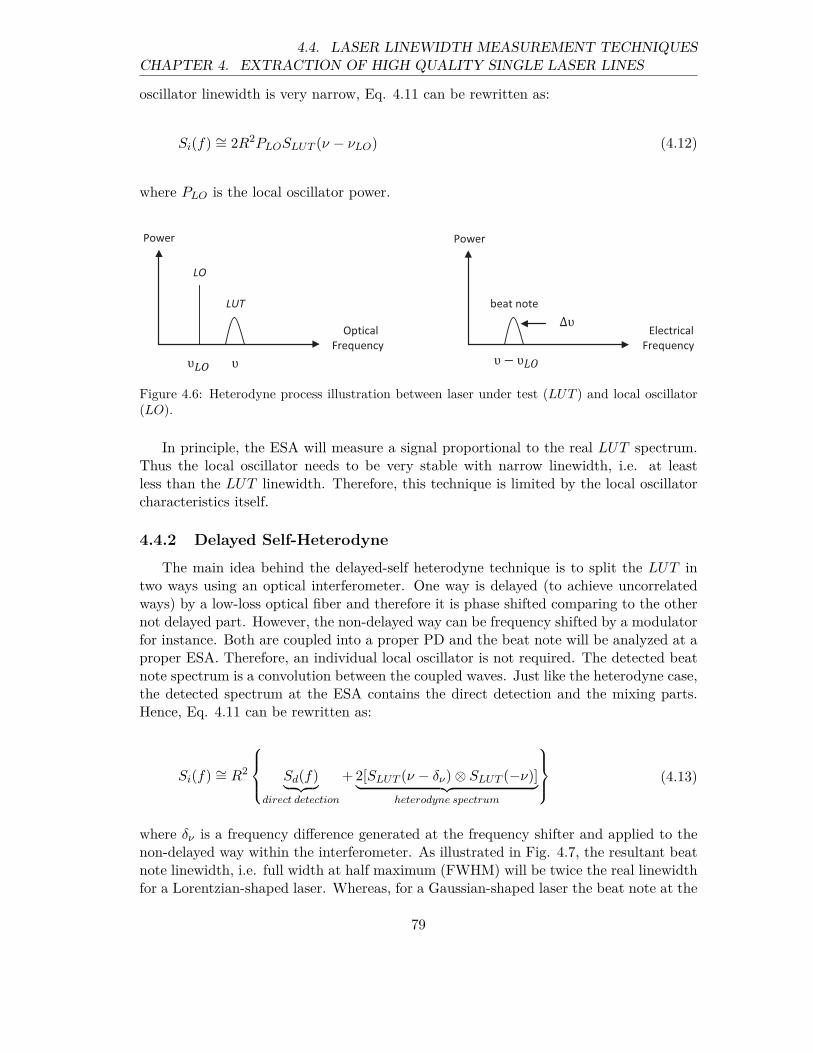
CHAPTER 4. EXTRACTION OF HIGH QUALITY SINGLE LASER LINES4.4. LASER LINEWIDTH MEASUREMENT TECHNIQUES
oscillator linewidth is very narrow, Eq. 4.11 can be rewritten as:
Si(f) ∼= 2R2PLOSLUT (ν − νLO) (4.12)
where PLO is the local oscillator power.
LO
LUT beat note
Power Power
Optical
Frequency
Electrical
Frequency
Figure 4.6: Heterodyne process illustration between laser under test (LUT ) and local oscillator(LO).
In principle, the ESA will measure a signal proportional to the real LUT spectrum.Thus the local oscillator needs to be very stable with narrow linewidth, i.e. at leastless than the LUT linewidth. Therefore, this technique is limited by the local oscillatorcharacteristics itself.
4.4.2 Delayed Self-Heterodyne
The main idea behind the delayed-self heterodyne technique is to split the LUT intwo ways using an optical interferometer. One way is delayed (to achieve uncorrelatedways) by a low-loss optical fiber and therefore it is phase shifted comparing to the othernot delayed part. However, the non-delayed way can be frequency shifted by a modulatorfor instance. Both are coupled into a proper PD and the beat note will be analyzed at aproper ESA. Therefore, an individual local oscillator is not required. The detected beatnote spectrum is a convolution between the coupled waves. Just like the heterodyne case,the detected spectrum at the ESA contains the direct detection and the mixing parts.Hence, Eq. 4.11 can be rewritten as:
Si(f) ∼= R2
Sd(f)︸ ︷︷ ︸direct detection
+ 2[SLUT (ν − δν) ⊗ SLUT (−ν)]︸ ︷︷ ︸heterodyne spectrum
(4.13)
where δν is a frequency difference generated at the frequency shifter and applied to thenon-delayed way within the interferometer. As illustrated in Fig. 4.7, the resultant beatnote linewidth, i.e. full width at half maximum (FWHM) will be twice the real linewidthfor a Lorentzian-shaped laser. Whereas, for a Gaussian-shaped laser the beat note at the
79
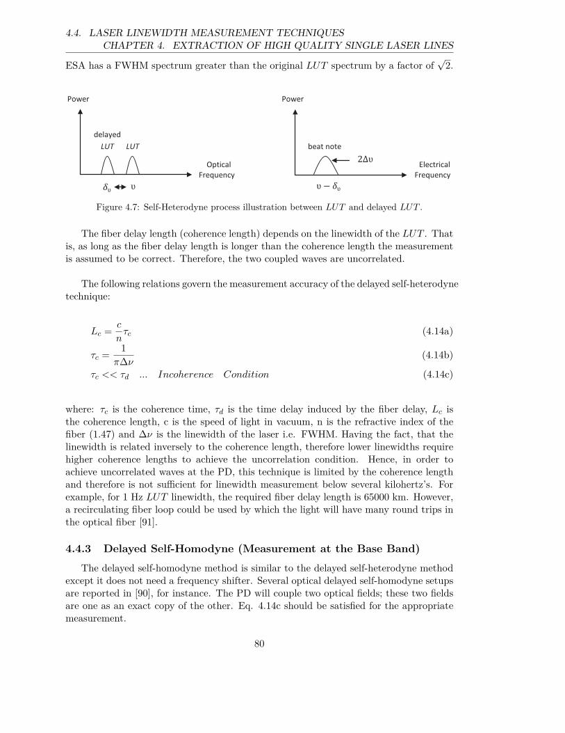
4.4. LASER LINEWIDTH MEASUREMENT TECHNIQUESCHAPTER 4. EXTRACTION OF HIGH QUALITY SINGLE LASER LINES
ESA has a FWHM spectrum greater than the original LUT spectrum by a factor of√
2.
delayed
LUT LUT beat note
2
Power Power
Optical
Frequency
Electrical
Frequency
Figure 4.7: Self-Heterodyne process illustration between LUT and delayed LUT .
The fiber delay length (coherence length) depends on the linewidth of the LUT . Thatis, as long as the fiber delay length is longer than the coherence length the measurementis assumed to be correct. Therefore, the two coupled waves are uncorrelated.
The following relations govern the measurement accuracy of the delayed self-heterodynetechnique:
Lc =c
nτc (4.14a)
τc =1
π∆ν(4.14b)
τc << τd ... Incoherence Condition (4.14c)
where: τc is the coherence time, τd is the time delay induced by the fiber delay, Lc isthe coherence length, c is the speed of light in vacuum, n is the refractive index of thefiber (1.47) and ∆ν is the linewidth of the laser i.e. FWHM. Having the fact, that thelinewidth is related inversely to the coherence length, therefore lower linewidths requirehigher coherence lengths to achieve the uncorrelation condition. Hence, in order toachieve uncorrelated waves at the PD, this technique is limited by the coherence lengthand therefore is not sufficient for linewidth measurement below several kilohertz’s. Forexample, for 1 Hz LUT linewidth, the required fiber delay length is 65000 km. However,a recirculating fiber loop could be used by which the light will have many round trips inthe optical fiber [91].
4.4.3 Delayed Self-Homodyne (Measurement at the Base Band)
The delayed self-homodyne method is similar to the delayed self-heterodyne methodexcept it does not need a frequency shifter. Several optical delayed self-homodyne setupsare reported in [90], for instance. The PD will couple two optical fields; these two fieldsare one as an exact copy of the other. Eq. 4.14c should be satisfied for the appropriatemeasurement.
80
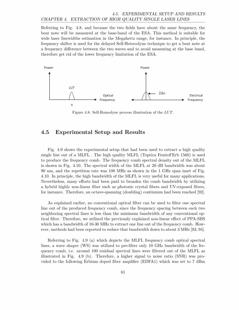
CHAPTER 4. EXTRACTION OF HIGH QUALITY SINGLE LASER LINES4.5. EXPERIMENTAL SETUP AND RESULTS
Referring to Fig. 4.8, and because the two fields have about the same frequency, thebeat note will be measured at the base-band of the ESA. This method is suitable forwide laser linewidths estimation in the Megahertz range, for instance. In principle, thefrequency shifter is used for the delayed Self-Heterodyne technique to get a beat note ata frequency difference between the two waves and to avoid measuring at the base band,therefore get rid of the lower frequency limitation of the ESA.
LUT
2
Power Power
Optical
Frequency
Electrical
Frequency
Figure 4.8: Self-Homodyne process illustration of the LUT .
4.5 Experimental Setup and Results
Fig. 4.9 shows the experimental setup that had been used to extract a high qualitysingle line out of a MLFL . The high quality MLFL (Toptica FemtoFErb 1560) is usedto produce the frequency comb. The frequency comb spectral density out of the MLFLis shown in Fig. 4.10. The spectral width of the MLFL at 20 dB bandwidth was about90 nm, and the repetition rate was 100 MHz as shown in the 1 GHz span inset of Fig.4.10. In principle, the high bandwidth of the MLFL is very useful for many applications.Nevertheless, many efforts had been paid to broaden the comb bandwidth by utilizinga hybrid highly non-linear fiber such as photonic crystal fibers and UV-exposed fibers,for instance. Therefore, an octave-spanning (doubling) continuum had been reached [92].
As explained earlier, no conventional optical filter can be used to filter one spectralline out of the produced frequency comb, since the frequency spacing between each twoneighboring spectral lines is less than the minimum bandwidth of any conventional op-tical filter. Therefore, we utilized the previously explained non-linear effect of PPA-SBSwhich has a bandwidth of 10-30 MHz to extract one line out of the frequency comb. How-ever, methods had been reported to reduce that bandwidth down to about 3 MHz [93, 94].
Referring to Fig. 4.9 (a) which depicts the MLFL frequency comb optical spectrallines, a wave shaper (WS) was utilized to pre-filter only 10 GHz bandwidth of the fre-quency comb, i.e. around 100 residual spectral lines were filtered out of the MLFL asillustrated in Fig. 4.9 (b). Therefore, a higher signal to noise ratio (SNR) was pro-vided to the following Erbium doped fiber amplifier (EDFA1) which was set to 7 dBm
81
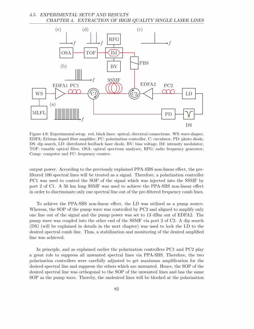
4.5. EXPERIMENTAL SETUP AND RESULTSCHAPTER 4. EXTRACTION OF HIGH QUALITY SINGLE LASER LINES
f
(a)
f
(b)
f
(c)
f
(d)
f
(e)
MLFL
WS
EDFA1 PC1
C1
SSMF
C2
EDFA2 PC2
LD
DS
PD
PBS
IMTOFOSA
RFG
BV
Figure 4.9: Experimental setup. red, black lines: optical, electrical connections. WS: wave shaper,EDFA: Erbium doped fiber amplifier, PC: polarization controller, C: circulator, PD: photo diode,DS: dip search, LD: distributed feedback laser diode, BV: bias voltage, IM: intensity modulator,TOF: tunable optical filter, OSA: optical spectrum analyzer, RFG: radio frequency generator,Comp: computer and FC: frequency counter.
output power. According to the previously explained PPA-SBS non-linear effect, the pre-filtered 100 spectral lines will be treated as a signal. Therefore, a polarization controllerPC1 was used to control the SOP of the signal which was injected into the SSMF byport 2 of C1. A 50 km long SSMF was used to achieve the PPA-SBS non-linear effectin order to discriminate only one spectral line out of the pre-filtered frequency comb lines.
To achieve the PPA-SBS non-linear effect, the LD was utilized as a pump source.Whereas, the SOP of the pump wave was controlled by PC2 and aligned to amplify onlyone line out of the signal and the pump power was set to 13 dBm out of EDFA2. Thepump wave was coupled into the other end of the SSMF via port 2 of C2. A dip search(DS) (will be explained in details in the next chapter) was used to lock the LD to thedesired spectral comb line. Thus, a stabilization and monitoring of the desired amplifiedline was achieved.
In principle, and as explained earlier the polarization controllers PC1 and PC2 playa great role to suppress all unwanted spectral lines via PPA-SBS. Therefore, the twopolarization controllers were carefully adjusted to get maximum amplification for thedesired spectral line and suppress the others which are unwanted. Hence, the SOP of thedesired spectral line was orthogonal to the SOP of the unwanted lines and has the sameSOP as the pump wave. Thereby, the undesired lines will be blocked at the polarization
82
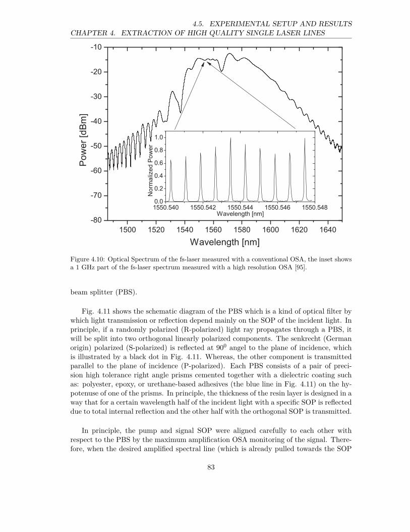
CHAPTER 4. EXTRACTION OF HIGH QUALITY SINGLE LASER LINES4.5. EXPERIMENTAL SETUP AND RESULTS
1500 1520 1540 1560 1580 1600 1620 1640
-80
-70
-60
-50
-40
-30
-20
-10
1550.540 1550.542 1550.544 1550.546 1550.5480.0
0.2
0.4
0.6
0.8
1.0
Power[dBm]
Wavelength [nm]
NormalizedPower
Wavelength [nm]
Figure 4.10: Optical Spectrum of the fs-laser measured with a conventional OSA, the inset showsa 1 GHz part of the fs-laser spectrum measured with a high resolution OSA [95].
beam splitter (PBS).
Fig. 4.11 shows the schematic diagram of the PBS which is a kind of optical filter bywhich light transmission or reflection depend mainly on the SOP of the incident light. Inprinciple, if a randomly polarized (R-polarized) light ray propagates through a PBS, itwill be split into two orthogonal linearly polarized components. The senkrecht (Germanorigin) polarized (S-polarized) is reflected at 900 angel to the plane of incidence, whichis illustrated by a black dot in Fig. 4.11. Whereas, the other component is transmittedparallel to the plane of incidence (P-polarized). Each PBS consists of a pair of preci-sion high tolerance right angle prisms cemented together with a dielectric coating suchas: polyester, epoxy, or urethane-based adhesives (the blue line in Fig. 4.11) on the hy-potenuse of one of the prisms. In principle, the thickness of the resin layer is designed in away that for a certain wavelength half of the incident light with a specific SOP is reflecteddue to total internal reflection and the other half with the orthogonal SOP is transmitted.
In principle, the pump and signal SOP were aligned carefully to each other withrespect to the PBS by the maximum amplification OSA monitoring of the signal. There-fore, when the desired amplified spectral line (which is already pulled towards the SOP
83
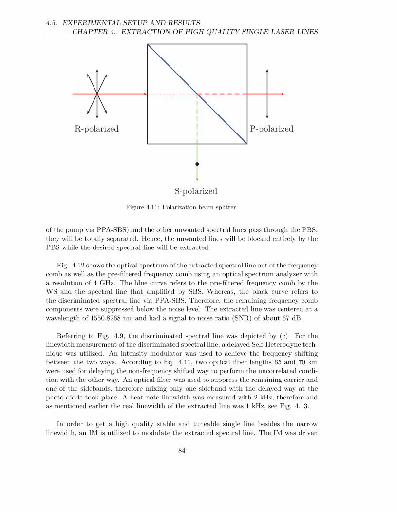
4.5. EXPERIMENTAL SETUP AND RESULTSCHAPTER 4. EXTRACTION OF HIGH QUALITY SINGLE LASER LINES
P-polarized
S-polarized
R-polarized
Figure 4.11: Polarization beam splitter.
of the pump via PPA-SBS) and the other unwanted spectral lines pass through the PBS,they will be totally separated. Hence, the unwanted lines will be blocked entirely by thePBS while the desired spectral line will be extracted.
Fig. 4.12 shows the optical spectrum of the extracted spectral line out of the frequencycomb as well as the pre-filtered frequency comb using an optical spectrum analyzer witha resolution of 4 GHz. The blue curve refers to the pre-filtered frequency comb by theWS and the spectral line that amplified by SBS. Whereas, the black curve refers tothe discriminated spectral line via PPA-SBS. Therefore, the remaining frequency combcomponents were suppressed below the noise level. The extracted line was centered at awavelength of 1550.8268 nm and had a signal to noise ratio (SNR) of about 67 dB.
Referring to Fig. 4.9, the discriminated spectral line was depicted by (c). For thelinewidth measurement of the discriminated spectral line, a delayed Self-Heterodyne tech-nique was utilized. An intensity modulator was used to achieve the frequency shiftingbetween the two ways. According to Eq. 4.11, two optical fiber lengths 65 and 70 kmwere used for delaying the non-frequency shifted way to perform the uncorrelated condi-tion with the other way. An optical filter was used to suppress the remaining carrier andone of the sidebands, therefore mixing only one sideband with the delayed way at thephoto diode took place. A beat note linewidth was measured with 2 kHz, therefore andas mentioned earlier the real linewidth of the extracted line was 1 kHz, see Fig. 4.13.
In order to get a high quality stable and tuneable single line besides the narrowlinewidth, an IM is utilized to modulate the extracted spectral line. The IM was driven
84

CHAPTER 4. EXTRACTION OF HIGH QUALITY SINGLE LASER LINES4.5. EXPERIMENTAL SETUP AND RESULTS
1550.1 1550.4 1550.7 1551.0 1551.3 1551.6-80
-70
-60
-50
-40
-30
-20
-10
0
Pow
er [d
Bm]
Wavelength [nm]
PPA-SBS SBS-only
Figure 4.12: Optical spectrum of the pre-filtered comb with a single line amplified by SBS (blue)and the suppression of the unwanted components through PPA-SBS (black). Please note thatthe linewidth of the spectral component is much narrower than the resolution bandwidth of theOSA.
in the carrier suppressed regime as illustrated in Fig. 4.9 (d). Therefore, the BV was setto 0.84 Vπ (3.2 V) and the RFG had been set to 17 dBm electrical output power. Asconsequence, only the first order sidebands had been achieved. As illustrated in Fig. 4.9(e), a TOF was utilized to filter only one sideband. The TOF had a bandwidth of 10GHz, therefore the modulation offset frequency was set to 5-20 GHz limited by the TOFand the IM bandwidths.
In order to show the ability for tuning the selected spectral line, it was modulatedwith 4 randomly chosen frequencies restricted by the 20 GHz bandwidth modulator. Fig.4.14 shows the optical spectrum of the modulated line with 5, 10, 15 and 20 GHz, theSNR was 47 dB at a limited conventional OSA resolution of 4 GHz. However, a verydelicate tuning can be achieved for full MLFL bandwidth by both: coarse and precisetuning of the extracted spectral line. For example, when the pump wave is shifted bychanging the laser diode current and locking to another spectral line via the DS tech-nique, then a coarse tuning will be achieved with a step of 100 MHz. Whereas, with the
85
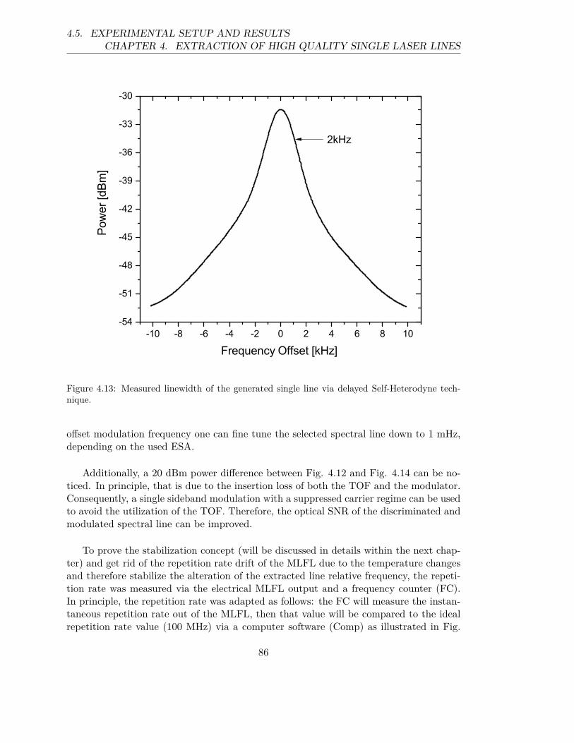
4.5. EXPERIMENTAL SETUP AND RESULTSCHAPTER 4. EXTRACTION OF HIGH QUALITY SINGLE LASER LINES
-10 -8 -6 -4 -2 0 2 4 6 8 10-54
-51
-48
-45
-42
-39
-36
-33
-30Po
wer
[dBm
]
Frequency Offset [kHz]
2kHz
Figure 4.13: Measured linewidth of the generated single line via delayed Self-Heterodyne tech-nique.
offset modulation frequency one can fine tune the selected spectral line down to 1 mHz,depending on the used ESA.
Additionally, a 20 dBm power difference between Fig. 4.12 and Fig. 4.14 can be no-ticed. In principle, that is due to the insertion loss of both the TOF and the modulator.Consequently, a single sideband modulation with a suppressed carrier regime can be usedto avoid the utilization of the TOF. Therefore, the optical SNR of the discriminated andmodulated spectral line can be improved.
To prove the stabilization concept (will be discussed in details within the next chap-ter) and get rid of the repetition rate drift of the MLFL due to the temperature changesand therefore stabilize the alteration of the extracted line relative frequency, the repeti-tion rate was measured via the electrical MLFL output and a frequency counter (FC).In principle, the repetition rate was adapted as follows: the FC will measure the instan-taneous repetition rate out of the MLFL, then that value will be compared to the idealrepetition rate value (100 MHz) via a computer software (Comp) as illustrated in Fig.
86

CHAPTER 4. EXTRACTION OF HIGH QUALITY SINGLE LASER LINES4.5. EXPERIMENTAL SETUP AND RESULTS
1551.1 1551.2 1551.3 1551.4 1551.5 1551.6
-80
-70
-60
-50
-40
-30
-20
Power[dBm]
Wavelength [nm]
05GHz
10GHz
15GHz
20GHz
Figure 4.14: Tuning of the discriminated line by different modulation frequencies.
4.9. The adaption value will be provided to the RFG to set the adaption frequency offsetfor the IM. For example, if the repetition rate is increased then the adaption frequencyoffset will decrease and vice versa. Therefore, the resultant sideband (single line) fre-quency will be adapted depending on the repetition rate alteration.
Fig. 4.15 shows the heterodyne beat note between the adapted spectral line with another extracted line out of the frequency comb. The 10 dB power difference between Fig.4.13 and Fig. 4.9 is due to the power loss within the IM and TOF.
87

4.6. SUMMARYCHAPTER 4. EXTRACTION OF HIGH QUALITY SINGLE LASER LINES
-1500 -1000 -500 0 500 1000 1500
-120
-110
-100
-90
-80
-70
-60
-50
Power[dBm]
Frequency Offset [Hz]
80Hz
Figure 4.15: Frequency shift of the heterodyned stabilized laser line and other spectral comb lineat a PD over 5 hours.
The beating frequency was centered at 24.63937142 GHz, i.e. there were 246 linesbetween the two mixed lines at the PD, and the drift was about 80 Hz over 5 hours.Consequently, the residual single line drift can be found by dividing the overall frequencydrift over the number of lines in between, i.e. 246. Thus, the resultant residual spectralline drift was ± 160 mHz.
4.6 Summary
The experimental setup is based on a stable, easy to operate, small footprint, light-weight and cost-effective MLFL as well as standard optical communications equipments.A highly stable, widely tuneable and extremely narrow single line laser was proposedand experimentally demonstrated. The precise stability of the extracted spectral linehad been achieved via measuring the repetition rate drift of the MLFL and an adapta-tion of the modulation frequency offset. Hence, the residual spectral line drift was ±160 mHz. However, the utilized stabilization technique was limited down to 100 mHzregistration value by the accuracy and the read out time of the FC. Therefore, during thestabilization process if faster repetition rate changes out of the MLL take place, then itcannot be captured. Thus, by a direct generation of the modulation frequency depend-
88

CHAPTER 4. EXTRACTION OF HIGH QUALITY SINGLE LASER LINES4.6. SUMMARY
ing on the directly measured repetition rate out of the MLFL with an analog circuit,that residual frequency drift could be largely reduced within the limits of the electricalcomponents [96]. Additionally, changing in the absolute frequency of the extracted linecould take place as well due to the whole laser drift. Nevertheless, in [97] several wellknown methods for femtosecond laser stabilization were reported.
The tuneability concept was proved via modulation frequency offset by randomlychoosing values limited by the modulator and the TOF. However, the discriminated sin-gle line laser can be easily tuned over the whole C-band via coarse and fine tuning, aswell as a tuneability over S-and L-bands could be achieved via non-linear comb broaden-ing. A linewidth of 1 kHz was measured as well as 47 dB SNR was achieved at a 4 GHzresolution OSA.
The high quality optical frequency comb out of the MLFL has wide application fieldslike: synthesis of ultra-purity optical and RF frequencies, metrology and precision spec-troscopy. The optical frequency comb out of the Toptica FemtoFErb 1560 femto-secondlaser was utilized to extract a high quality single spectral line. The PPA-SBS non-lineareffect was utilized as a sharp optical filter and amplifier to discriminate a high qualitysingle spectral line out of the optical frequency comb. The principle of operation of thePPA-SBS non-linear effect was explained. Additionally, several linewidth measurementtechniques were presented with their advantages and disadvantages. The delayed Self-Heterodyne was utilized to measure the linewidth of the extracted spectral line.
The implementation of the experimental setup for the single spectral line extraction,linewidth measurement, tuneability and stabilization were presented in detail. Amongthousands of spectral frequency comb lines only one line was discriminated via the PPA-SBS non-linear effect. The linewidth measurement of 1 kHz was achieved by the delayedSelf-Heterodyne technique. The fine tuneability with optical SNR of 47 dB was done bythe modulation, whereas the coarse tuning could easily be achieved by selecting anotherspectral line out of the frequency comb via PPA-SBS and therefore pump wavelengthtuning would be necessary. The residual stabilization of ± 160 mHz for the extractedlaser line was achieved by measuring the repetition rate out of the MLFL electrically andadapting it via computer software and modulation frequency.
The high quality and wide tuneability of the generated single line laser, shows highpotential for many applications in the field of optical communications with spectral effi-cient modulation formats and for ultra-high resolution spectroscopy.
89

4.6. SUMMARYCHAPTER 4. EXTRACTION OF HIGH QUALITY SINGLE LASER LINES
90
Chapter 5
High Quality Millimeter WaveGeneration
5.1 Introduction
The millimetre length electromagnetic waves were first investigated within the 1890sby pioneering Indian scientist Jagadish Chandra Bose. These waves travel just throughline-of-sight and are blocked via building walls and attenuated by foliage as well [98]. Inprinciple, the millimeter (30 - 300 GHz), i.e. (1 cm - 1 mm) and sub-millimeter or THzband (0.3 - 3 THz) of the electromagnetic spectrum has great potential for various sci-entific and engineering applications like photonic analog-to-digital converters [99], localoscillators for fountain clocks [100], high performance antennas and radars, high speedwireless communications, and high-resolution signal analysis. In wireless communicationsfor instance, the frequency bands above 300 GHz are unused and offer large bandwidthsfor transmissions up to the TBits/s range [101]. Additionally, the wide band provides avaluable support for video distribution and high speed data [102].
Usually, electrical oscillators are used for the generation of electrical waves in the MHzand GHz range, frequencies up to 100 GHz are actually possible. These frequencies canbe transferred into higher frequency ranges via electronic up conversions, the millimeterand sub-millimeter range, for instance. Unfortunately, the electronic upconversion gen-erates a phase noise which scales quadratically with the harmonic frequency order due tothe non-linear mixing processes [103]. Thus, millimeter wave generation with low phasenoise is challenging via electronic methods.
A more convenient approach for the millimeter wave generation is the heterodyningand optoelectronic conversion of two optical waves in an appropriate non-linear elementsuch as a non-linear crystal or a PD. For example, optical heterodyning of two inde-pendent laser sources is the simplest way to generate mm-waves with wide frequencytuneability. In [104] for example, a beat note of about 3.3 MHz linewidth was reported
91
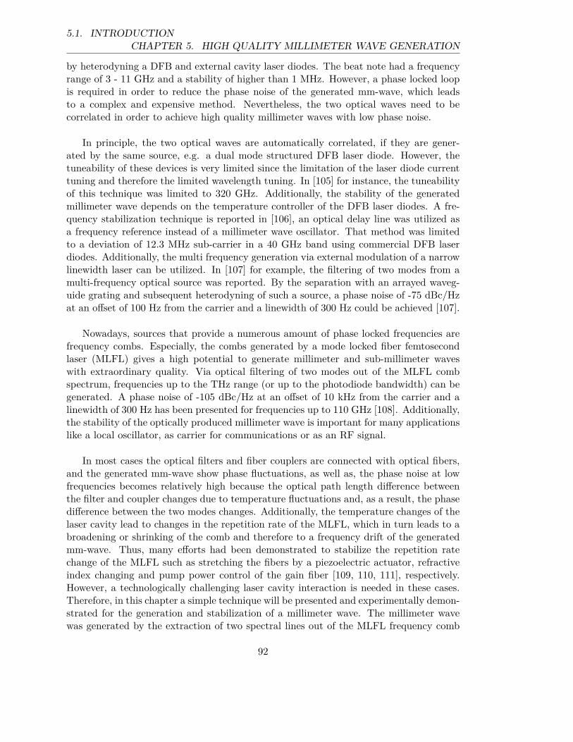
5.1. INTRODUCTIONCHAPTER 5. HIGH QUALITY MILLIMETER WAVE GENERATION
by heterodyning a DFB and external cavity laser diodes. The beat note had a frequencyrange of 3 - 11 GHz and a stability of higher than 1 MHz. However, a phase locked loopis required in order to reduce the phase noise of the generated mm-wave, which leadsto a complex and expensive method. Nevertheless, the two optical waves need to becorrelated in order to achieve high quality millimeter waves with low phase noise.
In principle, the two optical waves are automatically correlated, if they are gener-ated by the same source, e.g. a dual mode structured DFB laser diode. However, thetuneability of these devices is very limited since the limitation of the laser diode currenttuning and therefore the limited wavelength tuning. In [105] for instance, the tuneabilityof this technique was limited to 320 GHz. Additionally, the stability of the generatedmillimeter wave depends on the temperature controller of the DFB laser diodes. A fre-quency stabilization technique is reported in [106], an optical delay line was utilized asa frequency reference instead of a millimeter wave oscillator. That method was limitedto a deviation of 12.3 MHz sub-carrier in a 40 GHz band using commercial DFB laserdiodes. Additionally, the multi frequency generation via external modulation of a narrowlinewidth laser can be utilized. In [107] for example, the filtering of two modes from amulti-frequency optical source was reported. By the separation with an arrayed waveg-uide grating and subsequent heterodyning of such a source, a phase noise of -75 dBc/Hzat an offset of 100 Hz from the carrier and a linewidth of 300 Hz could be achieved [107].
Nowadays, sources that provide a numerous amount of phase locked frequencies arefrequency combs. Especially, the combs generated by a mode locked fiber femtosecondlaser (MLFL) gives a high potential to generate millimeter and sub-millimeter waveswith extraordinary quality. Via optical filtering of two modes out of the MLFL combspectrum, frequencies up to the THz range (or up to the photodiode bandwidth) can begenerated. A phase noise of -105 dBc/Hz at an offset of 10 kHz from the carrier and alinewidth of 300 Hz has been presented for frequencies up to 110 GHz [108]. Additionally,the stability of the optically produced millimeter wave is important for many applicationslike a local oscillator, as carrier for communications or as an RF signal.
In most cases the optical filters and fiber couplers are connected with optical fibers,and the generated mm-wave show phase fluctuations, as well as, the phase noise at lowfrequencies becomes relatively high because the optical path length difference betweenthe filter and coupler changes due to temperature fluctuations and, as a result, the phasedifference between the two modes changes. Additionally, the temperature changes of thelaser cavity lead to changes in the repetition rate of the MLFL, which in turn leads to abroadening or shrinking of the comb and therefore to a frequency drift of the generatedmm-wave. Thus, many efforts had been demonstrated to stabilize the repetition ratechange of the MLFL such as stretching the fibers by a piezoelectric actuator, refractiveindex changing and pump power control of the gain fiber [109, 110, 111], respectively.However, a technologically challenging laser cavity interaction is needed in these cases.Therefore, in this chapter a simple technique will be presented and experimentally demon-strated for the generation and stabilization of a millimeter wave. The millimeter wavewas generated by the extraction of two spectral lines out of the MLFL frequency comb
92

CHAPTER 5. HIGH QUALITY MILLIMETER WAVE GENERATION5.2. MILLIMETER-WAVE GENERATION BY MIXING TWO OPTICAL WAVES
and both were mixed at a proper PD. The stabilization was achieved by the stabilizationof the MLFL repetition rate via two approaches: analog and software, without an inter-action with the laser cavity, and therefore the generated millimeter wave was stabilized aswell. Thus, one of the optical waves is externally modulated and adapted at the inverseof the repetition rate drift. An analog and software approach for the generation of themodulation signal are presented and compared.
This chapter is organized as follows: the description of mm-wave generation from themixing of two optical waves as well as the phase noise are presented. An elegant methodto generate and stabilize a high quality mm-wave with low phase noise via extracting twospectral lines out of a frequency comb is explained. Then the experimental setup andresults are presented.
5.2 Millimeter-Wave Generation by Mixing Two OpticalWaves
Currently, the mixing and optoelectronic conversion of two optical waves at a properPD is a widely used method for the generation of mm-waves. Fig. 5.1 illustrates themixing of two different optical frequencies at a non-linear element (PD), the gray arrowsare referring to the frequency drifting.
PD
f1
f2
f3
Figure 5.1: Schematic diagram for mm-wave generation by difference frequency generation. Thetwo optical fields are heterodyned at a photo diode (PD).
Referring to Fig. 5.1, the electrical fields of the two optical input waves (f1, f2) canbe written as [90]:
E1(t) = |E1(t)| cos (ω1t) (5.1a)
E2(t) = |E2(t)| cos (ω2t+ φ) (5.1b)
93
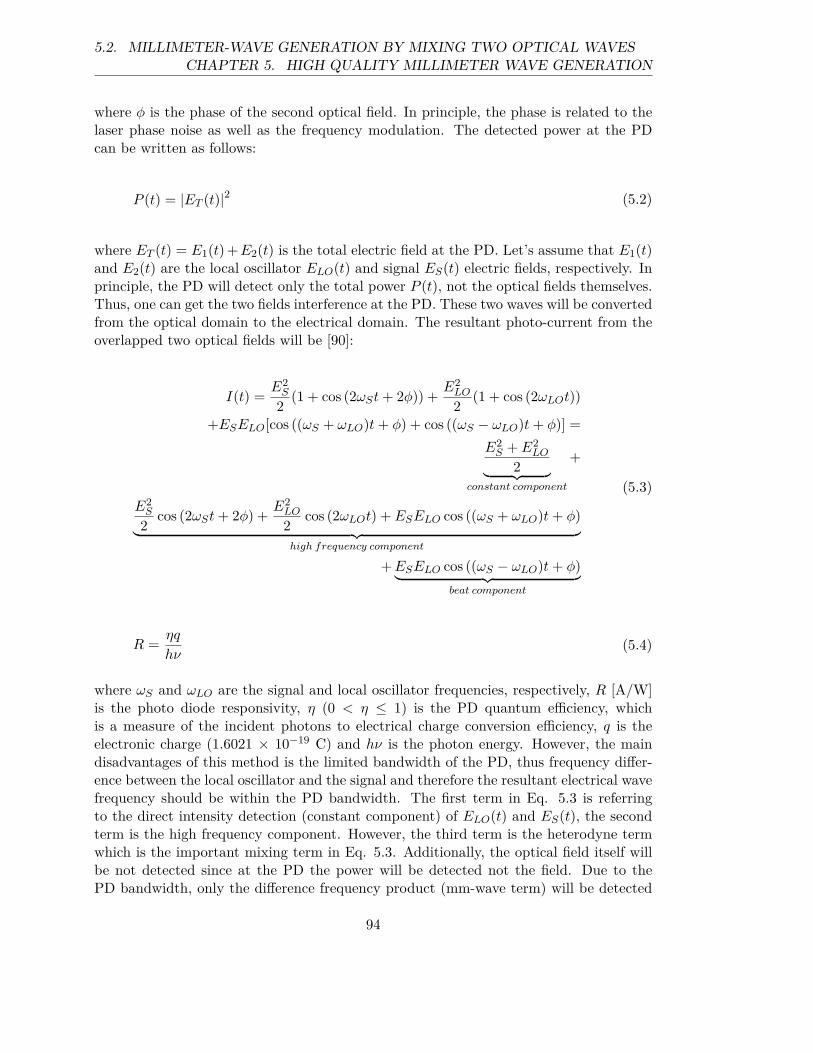
5.2. MILLIMETER-WAVE GENERATION BY MIXING TWO OPTICAL WAVESCHAPTER 5. HIGH QUALITY MILLIMETER WAVE GENERATION
where φ is the phase of the second optical field. In principle, the phase is related to thelaser phase noise as well as the frequency modulation. The detected power at the PDcan be written as follows:
P (t) = |ET (t)|2 (5.2)
where ET (t) = E1(t) +E2(t) is the total electric field at the PD. Let’s assume that E1(t)and E2(t) are the local oscillator ELO(t) and signal ES(t) electric fields, respectively. Inprinciple, the PD will detect only the total power P (t), not the optical fields themselves.Thus, one can get the two fields interference at the PD. These two waves will be convertedfrom the optical domain to the electrical domain. The resultant photo-current from theoverlapped two optical fields will be [90]:
I(t) =E2
S
2(1 + cos (2ωSt+ 2φ)) +
E2LO
2(1 + cos (2ωLOt))
+ESELO[cos ((ωS + ωLO)t+ φ) + cos ((ωS − ωLO)t+ φ)] =
E2S + E2
LO
2︸ ︷︷ ︸constant component
+
E2S
2cos (2ωSt+ 2φ) +
E2LO
2cos (2ωLOt) + ESELO cos ((ωS + ωLO)t+ φ)
︸ ︷︷ ︸high frequency component
+ESELO cos ((ωS − ωLO)t+ φ)︸ ︷︷ ︸beat component
(5.3)
R =ηq
hν(5.4)
where ωS and ωLO are the signal and local oscillator frequencies, respectively, R [A/W]is the photo diode responsivity, η (0 < η ≤ 1) is the PD quantum efficiency, whichis a measure of the incident photons to electrical charge conversion efficiency, q is theelectronic charge (1.6021 × 10⁻¹⁹ C) and hν is the photon energy. However, the maindisadvantages of this method is the limited bandwidth of the PD, thus frequency differ-ence between the local oscillator and the signal and therefore the resultant electrical wavefrequency should be within the PD bandwidth. The first term in Eq. 5.3 is referringto the direct intensity detection (constant component) of ELO(t) and ES(t), the secondterm is the high frequency component. However, the third term is the heterodyne termwhich is the important mixing term in Eq. 5.3. Additionally, the optical field itself willbe not detected since at the PD the power will be detected not the field. Due to thePD bandwidth, only the difference frequency product (mm-wave term) will be detected
94
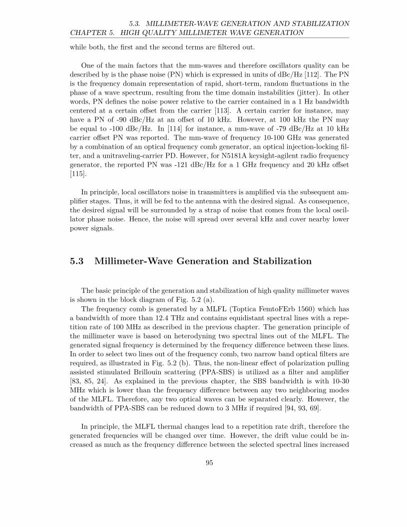
CHAPTER 5. HIGH QUALITY MILLIMETER WAVE GENERATION5.3. MILLIMETER-WAVE GENERATION AND STABILIZATION
while both, the first and the second terms are filtered out.
One of the main factors that the mm-waves and therefore oscillators quality can bedescribed by is the phase noise (PN) which is expressed in units of dBc/Hz [112]. The PNis the frequency domain representation of rapid, short-term, random fluctuations in thephase of a wave spectrum, resulting from the time domain instabilities (jitter). In otherwords, PN defines the noise power relative to the carrier contained in a 1 Hz bandwidthcentered at a certain offset from the carrier [113]. A certain carrier for instance, mayhave a PN of -90 dBc/Hz at an offset of 10 kHz. However, at 100 kHz the PN maybe equal to -100 dBc/Hz. In [114] for instance, a mm-wave of -79 dBc/Hz at 10 kHzcarrier offset PN was reported. The mm-wave of frequency 10-100 GHz was generatedby a combination of an optical frequency comb generator, an optical injection-locking fil-ter, and a unitraveling-carrier PD. However, for N5181A keysight-agilent radio frequencygenerator, the reported PN was -121 dBc/Hz for a 1 GHz frequency and 20 kHz offset[115].
In principle, local oscillators noise in transmitters is amplified via the subsequent am-plifier stages. Thus, it will be fed to the antenna with the desired signal. As consequence,the desired signal will be surrounded by a strap of noise that comes from the local oscil-lator phase noise. Hence, the noise will spread over several kHz and cover nearby lowerpower signals.
5.3 Millimeter-Wave Generation and Stabilization
The basic principle of the generation and stabilization of high quality millimeter wavesis shown in the block diagram of Fig. 5.2 (a).
The frequency comb is generated by a MLFL (Toptica FemtoFErb 1560) which hasa bandwidth of more than 12.4 THz and contains equidistant spectral lines with a repe-tition rate of 100 MHz as described in the previous chapter. The generation principle ofthe millimeter wave is based on heterodyning two spectral lines out of the MLFL. Thegenerated signal frequency is determined by the frequency difference between these lines.In order to select two lines out of the frequency comb, two narrow band optical filters arerequired, as illustrated in Fig. 5.2 (b). Thus, the non-linear effect of polarization pullingassisted stimulated Brillouin scattering (PPA-SBS) is utilized as a filter and amplifier[83, 85, 24]. As explained in the previous chapter, the SBS bandwidth is with 10-30MHz which is lower than the frequency difference between any two neighboring modesof the MLFL. Therefore, any two optical waves can be separated clearly. However, thebandwidth of PPA-SBS can be reduced down to 3 MHz if required [94, 93, 69].
In principle, the MLFL thermal changes lead to a repetition rate drift, therefore thegenerated frequencies will be changed over time. However, the drift value could be in-creased as much as the frequency difference between the selected spectral lines increased
95
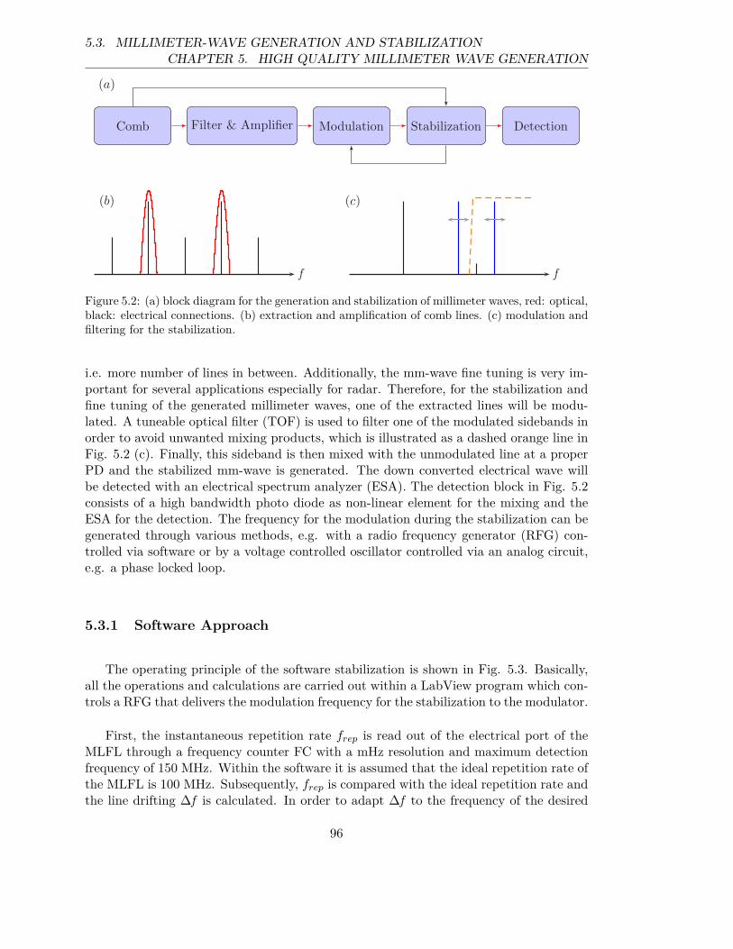
5.3. MILLIMETER-WAVE GENERATION AND STABILIZATIONCHAPTER 5. HIGH QUALITY MILLIMETER WAVE GENERATION
Comb Filter & Amplifier Modulation Stabilization Detection
f f
(b) (c)
(a)
Figure 5.2: (a) block diagram for the generation and stabilization of millimeter waves, red: optical,black: electrical connections. (b) extraction and amplification of comb lines. (c) modulation andfiltering for the stabilization.
i.e. more number of lines in between. Additionally, the mm-wave fine tuning is very im-portant for several applications especially for radar. Therefore, for the stabilization andfine tuning of the generated millimeter waves, one of the extracted lines will be modu-lated. A tuneable optical filter (TOF) is used to filter one of the modulated sidebands inorder to avoid unwanted mixing products, which is illustrated as a dashed orange line inFig. 5.2 (c). Finally, this sideband is then mixed with the unmodulated line at a properPD and the stabilized mm-wave is generated. The down converted electrical wave willbe detected with an electrical spectrum analyzer (ESA). The detection block in Fig. 5.2consists of a high bandwidth photo diode as non-linear element for the mixing and theESA for the detection. The frequency for the modulation during the stabilization can begenerated through various methods, e.g. with a radio frequency generator (RFG) con-trolled via software or by a voltage controlled oscillator controlled via an analog circuit,e.g. a phase locked loop.
5.3.1 Software Approach
The operating principle of the software stabilization is shown in Fig. 5.3. Basically,all the operations and calculations are carried out within a LabView program which con-trols a RFG that delivers the modulation frequency for the stabilization to the modulator.
First, the instantaneous repetition rate frep is read out of the electrical port of theMLFL through a frequency counter FC with a mHz resolution and maximum detectionfrequency of 150 MHz. Within the software it is assumed that the ideal repetition rate ofthe MLFL is 100 MHz. Subsequently, frep is compared with the ideal repetition rate andthe line drifting ∆f is calculated. In order to adapt ∆f to the frequency of the desired
96
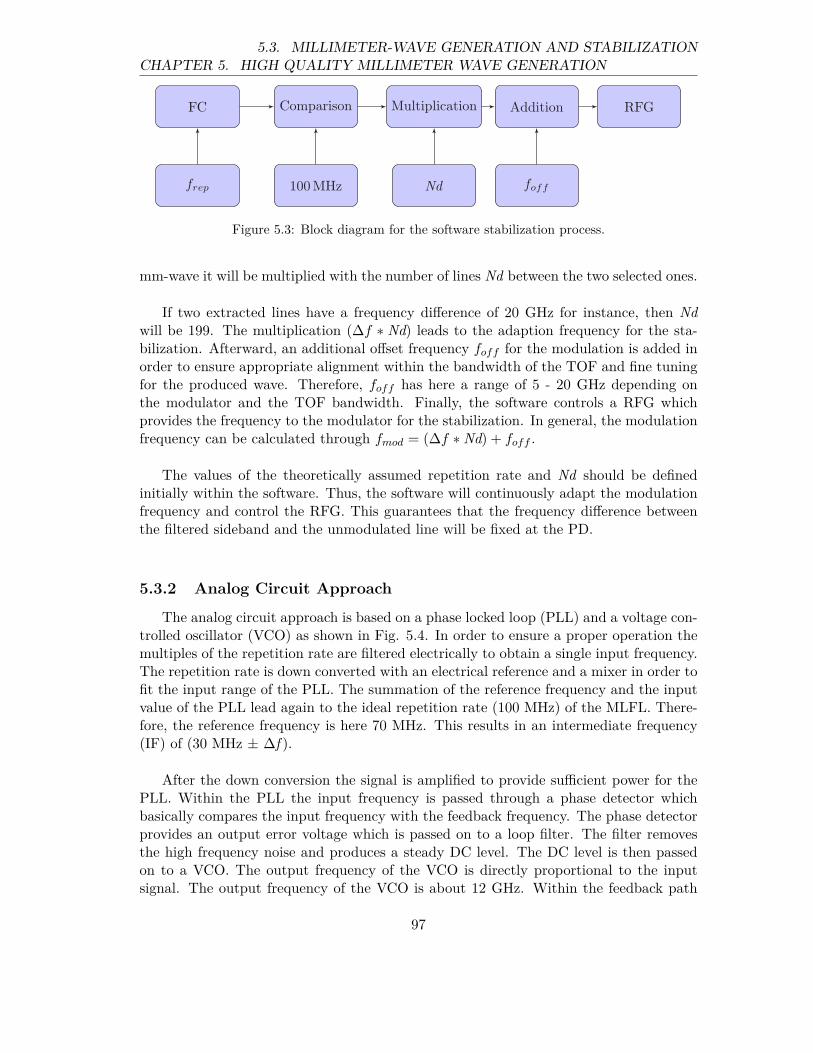
CHAPTER 5. HIGH QUALITY MILLIMETER WAVE GENERATION5.3. MILLIMETER-WAVE GENERATION AND STABILIZATION
FC
frep
Comparison Multiplication
100MHz Nd
Addition
foff
RFG
Figure 5.3: Block diagram for the software stabilization process.
mm-wave it will be multiplied with the number of lines Nd between the two selected ones.
If two extracted lines have a frequency difference of 20 GHz for instance, then Nd
will be 199. The multiplication (∆f ∗ Nd) leads to the adaption frequency for the sta-bilization. Afterward, an additional offset frequency foff for the modulation is added inorder to ensure appropriate alignment within the bandwidth of the TOF and fine tuningfor the produced wave. Therefore, foff has here a range of 5 - 20 GHz depending onthe modulator and the TOF bandwidth. Finally, the software controls a RFG whichprovides the frequency to the modulator for the stabilization. In general, the modulationfrequency can be calculated through fmod = (∆f ∗ Nd) + foff .
The values of the theoretically assumed repetition rate and Nd should be definedinitially within the software. Thus, the software will continuously adapt the modulationfrequency and control the RFG. This guarantees that the frequency difference betweenthe filtered sideband and the unmodulated line will be fixed at the PD.
5.3.2 Analog Circuit Approach
The analog circuit approach is based on a phase locked loop (PLL) and a voltage con-trolled oscillator (VCO) as shown in Fig. 5.4. In order to ensure a proper operation themultiples of the repetition rate are filtered electrically to obtain a single input frequency.The repetition rate is down converted with an electrical reference and a mixer in order tofit the input range of the PLL. The summation of the reference frequency and the inputvalue of the PLL lead again to the ideal repetition rate (100 MHz) of the MLFL. There-fore, the reference frequency is here 70 MHz. This results in an intermediate frequency(IF) of (30 MHz ± ∆f ).
After the down conversion the signal is amplified to provide sufficient power for thePLL. Within the PLL the input frequency is passed through a phase detector whichbasically compares the input frequency with the feedback frequency. The phase detectorprovides an output error voltage which is passed on to a loop filter. The filter removesthe high frequency noise and produces a steady DC level. The DC level is then passedon to a VCO. The output frequency of the VCO is directly proportional to the inputsignal. The output frequency of the VCO is about 12 GHz. Within the feedback path
97

5.4. EXPERIMENTAL SETUP AND RESULTSCHAPTER 5. HIGH QUALITY MILLIMETER WAVE GENERATION
PLL
frepIFRF
LO
70MHz
PhaseDetector
LoopFilter
VCOf
Freq. Divider: Nd
•
Figure 5.4: Operating principle of the analog circuit.
the output frequency of the VCO is divided by the number of lines Nd. Therefore, thefeedback frequency fits again the input range.
Both, the input frequency and feedback frequency are compared and adjusted throughfeedback loops until the output frequency equals the input frequency. Thus, changes ofthe repetition rate are directly translated to a change of the VCO output frequency, whichdrives the modulator for the stabilization. Again, this leads to a very stable mm-waveafter the down conversion of the two optical waves. To provide sufficient power for themodulator, the VCO output signal is amplified. Since the output range of the PLL isaround 12 GHz there is no additional offset frequency necessary. The unwanted sidebandof the modulation can be filtered out easily with the TOF.
5.4 Experimental Setup and Results
The experimental setup is shown in Fig. 5.5 [25]. As explained in the previous section,for the extraction of two lines out of the MLFL frequency comb, the non-linear effect ofPPA-SBS is used [116] as illustrated in Fig. 5.5 (dashed box).
The frequency comb will be pre-filtered by a 10 GHz bandwidth wave shaper WS.The state of polarization (SOP) of the pre-filtered spectral lines (treated as a signal forthe SBS process) will be controlled via a PC. The signal will be launched to the 20 kmSSMF via port 2 of C1, while the two pump waves from LD1 and LD2 will be launchedto the other end of the SSMF via port 2 of C2 and their SOP will be controlled via twopolarization controllers PC.
In principle, in order to lock the two laser diodes LD1 and LD2 to the desired twospectral comb lines through the SBS process, an electrical dip search (DS) module, i.eminimum value detection was utilized [117]. Within SBS process and as explained inchapter two, the pump power will be transferred to the amplified signal. Therefore, anarrow band and fast PD1 was used to detect the pump power out of the SSMF via port3 of C1. Thus, the DS module will trace the maximum pump power depletion (signal
98
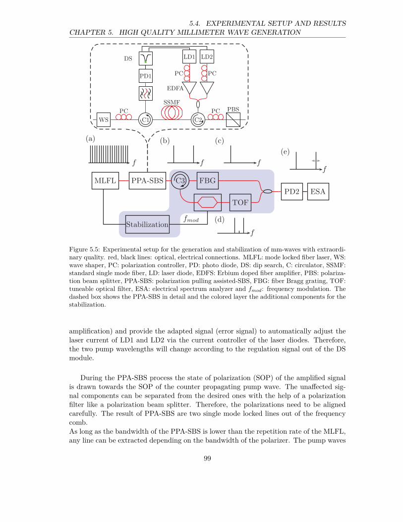
CHAPTER 5. HIGH QUALITY MILLIMETER WAVE GENERATION5.4. EXPERIMENTAL SETUP AND RESULTS
MLFL PPA-SBS C3 FBG
TOF
PD2 ESA
Stabilizationfmod
f
(a)
f
(b)
f
(c)
f
(d)
f
(e)
PC
C1
SSMF
C2
PC PBS
EDFA
PCPC
LD2LD1
PD1
DS
WS
Figure 5.5: Experimental setup for the generation and stabilization of mm-waves with extraordi-nary quality. red, black lines: optical, electrical connections. MLFL: mode locked fiber laser, WS:wave shaper, PC: polarization controller, PD: photo diode, DS: dip search, C: circulator, SSMF:standard single mode fiber, LD: laser diode, EDFS: Erbium doped fiber amplifier, PBS: polariza-tion beam splitter, PPA-SBS: polarization pulling assisted-SBS, FBG: fiber Bragg grating, TOF:tuneable optical filter, ESA: electrical spectrum analyzer and fmod: frequency modulation. Thedashed box shows the PPA-SBS in detail and the colored layer the additional components for thestabilization.
amplification) and provide the adapted signal (error signal) to automatically adjust thelaser current of LD1 and LD2 via the current controller of the laser diodes. Therefore,the two pump wavelengths will change according to the regulation signal out of the DSmodule.
During the PPA-SBS process the state of polarization (SOP) of the amplified signalis drawn towards the SOP of the counter propagating pump wave. The unaffected sig-nal components can be separated from the desired ones with the help of a polarizationfilter like a polarization beam splitter. Therefore, the polarizations need to be alignedcarefully. The result of PPA-SBS are two single mode locked lines out of the frequencycomb.As long as the bandwidth of the PPA-SBS is lower than the repetition rate of the MLFL,any line can be extracted depending on the bandwidth of the polarizer. The pump waves
99
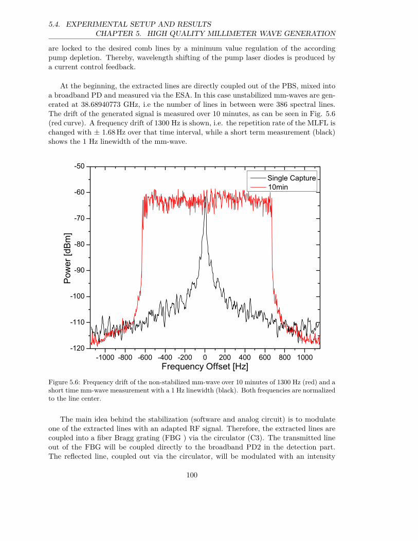
5.4. EXPERIMENTAL SETUP AND RESULTSCHAPTER 5. HIGH QUALITY MILLIMETER WAVE GENERATION
are locked to the desired comb lines by a minimum value regulation of the accordingpump depletion. Thereby, wavelength shifting of the pump laser diodes is produced bya current control feedback.
At the beginning, the extracted lines are directly coupled out of the PBS, mixed intoa broadband PD and measured via the ESA. In this case unstabilized mm-waves are gen-erated at 38.68940773 GHz, i.e the number of lines in between were 386 spectral lines.The drift of the generated signal is measured over 10 minutes, as can be seen in Fig. 5.6(red curve). A frequency drift of 1300 Hz is shown, i.e. the repetition rate of the MLFL ischanged with ± 1.68 Hz over that time interval, while a short term measurement (black)shows the 1 Hz linewidth of the mm-wave.
-1000 -800 -600 -400 -200 0 200 400 600 800 1000
-120
-110
-100
-90
-80
-70
-60
-50
Power[dBm]
Frequency Offset [Hz]
Single Capture
10min
Figure 5.6: Frequency drift of the non-stabilized mm-wave over 10 minutes of 1300 Hz (red) and ashort time mm-wave measurement with a 1 Hz linewidth (black). Both frequencies are normalizedto the line center.
The main idea behind the stabilization (software and analog circuit) is to modulateone of the extracted lines with an adapted RF signal. Therefore, the extracted lines arecoupled into a fiber Bragg grating (FBG ) via the circulator (C3). The transmitted lineout of the FBG will be coupled directly to the broadband PD2 in the detection part.The reflected line, coupled out via the circulator, will be modulated with an intensity
100
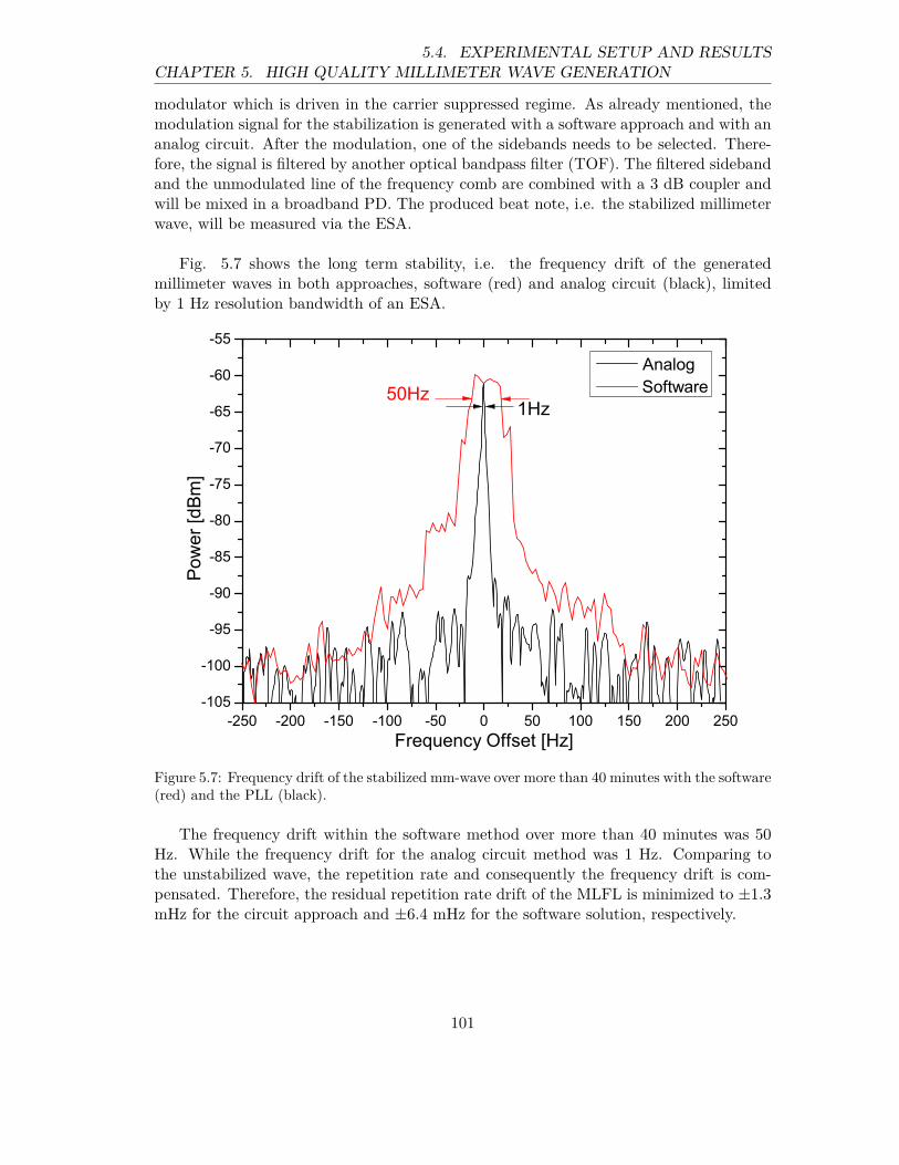
CHAPTER 5. HIGH QUALITY MILLIMETER WAVE GENERATION5.4. EXPERIMENTAL SETUP AND RESULTS
modulator which is driven in the carrier suppressed regime. As already mentioned, themodulation signal for the stabilization is generated with a software approach and with ananalog circuit. After the modulation, one of the sidebands needs to be selected. There-fore, the signal is filtered by another optical bandpass filter (TOF). The filtered sidebandand the unmodulated line of the frequency comb are combined with a 3 dB coupler andwill be mixed in a broadband PD. The produced beat note, i.e. the stabilized millimeterwave, will be measured via the ESA.
Fig. 5.7 shows the long term stability, i.e. the frequency drift of the generatedmillimeter waves in both approaches, software (red) and analog circuit (black), limitedby 1 Hz resolution bandwidth of an ESA.
-250 -200 -150 -100 -50 0 50 100 150 200 250
-105
-100
-95
-90
-85
-80
-75
-70
-65
-60
-55
1Hz
Power[dBm]
Frequency Offset [Hz]
Analog
Software50Hz
Figure 5.7: Frequency drift of the stabilized mm-wave over more than 40 minutes with the software(red) and the PLL (black).
The frequency drift within the software method over more than 40 minutes was 50Hz. While the frequency drift for the analog circuit method was 1 Hz. Comparing tothe unstabilized wave, the repetition rate and consequently the frequency drift is com-pensated. Therefore, the residual repetition rate drift of the MLFL is minimized to ±1.3mHz for the circuit approach and ±6.4 mHz for the software solution, respectively.
101
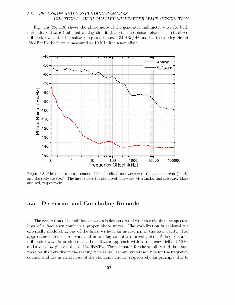
5.5. DISCUSSION AND CONCLUDING REMARKSCHAPTER 5. HIGH QUALITY MILLIMETER WAVE GENERATION
Fig. 5.8 [25, 118] shows the phase noise of the generated millimeter wave for bothmethods, software (red) and analog circuit (black). The phase noise of the stabilizedmillimeter wave for the software approach was -134 dBc/Hz and for the analog circuit-58 dBc/Hz, both were measured at 10 kHz frequency offset.
0.1 1 10 100 1000 10000 100000
-150
-140
-130
-120
-110
-100
-90
-80
-70
-60
-50
-40
PhaseNoise[dBc/Hz]
Frequency Offset [kHz]
Analog
Software
Figure 5.8: Phase noise measurement of the stabilized mm-wave with the analog circuit (black)and the software (red). The inset shows the stabilized mm-wave with analog and software: blackand red, respectively.
5.5 Discussion and Concluding Remarks
The generation of the millimeter waves is demonstrated via heterodyning two spectrallines of a frequency comb in a proper photo mixer. The stabilization is achieved viaexternally modulating one of the lines, without an interaction in the laser cavity. Twoapproaches based on software and an analog circuit are investigated. A highly stablemillimeter wave is produced via the software approach with a frequency drift of 50 Hzand a very low phase noise of -134 dBc/Hz. The mismatch for the stability and the phasenoise results were due to the reading time as well as minimum resolution for the frequencycounter and the internal noise of the electronic circuit, respectively. In principle, due to
102
CHAPTER 5. HIGH QUALITY MILLIMETER WAVE GENERATION5.6. SUMMARY
the electronic limitation of the VCO, the phase noise of the analog circuit was higherwhich is transferred to the modulation. While the long term stability was 1 Hz. At anyrate, this optical generation method provides high potential regarding the phase noiseand stability in a comparison with electrical signal generation methods, especially forhigher frequencies.
The two proposed mm-wave stabilization methods have their own benefits. However,the software stabilization technique for instance, had shown a much lower phase noiseachieved by the high quality RFG. Additionally, lower stability had been got due to thelimited resolution of the frequency counter and the slow read out rate, and thereforelimited update rate of the software-based control loop had been took place. Additionally,the software-stabilization technique is very useful for communication systems, since itslow phase noise. However, the 50 kHz drift range is insufficient, thus frequency stabiliza-tion by means of carrier recovery and synchronization mechanisms could be additionallyutilized, by which they are inherent part of the receiver and demodulator.
In principle, both: software and analog circuit approaches could be improved to getrid of the low resolution of the frequency counter and the high phase noise of the VCOas well as the limited input and output range of the PLL and therefore the tuneabilityrange. Hence, a high precision digital frequency counter or a higher quality VCO couldbe utilized. Additionally, the filtering of the mixing products is highly recommendedto get proper operations, since spurious frequencies could take place. The FC, softwareprocessing and controlling could be combined at a micro controller or integrating with afield programmable gate array (FPGA) to get rid of the timing challenges and thereforethe degradation of this method.
5.6 Summary
Highly quality millimeter-waves provide a great potential for several applicationswithin scientific research, telecommunications, security screening and medicine. There-fore, a novel stabilization technique for the generation of mm-waves has been proposedand experimentally proofed.
A basic theory about two optical wave mixing at a non-linear element such as aphoto diode to generate a proper RF signal was explained. Two spectral lines out of ahigh quality frequency comb produced by a femtosecond fiber laser were interfered togenerate the millimeter-wave. One of the extracted lines was modulated to stabilize themillimeter-wave, and therefore any modulation information could be added to the mod-ulated mode. Thus, the repetition rate drift could be overcame. Additionally, choosingvariable wavelength laser modes from the MLFL permits flexible and tunable RF signalsgeneration.
Two mm-wave stabilization approaches: software and analog were experimentallydemonstrated that can produce high quality mm-waves. Within the software approach
103

5.6. SUMMARYCHAPTER 5. HIGH QUALITY MILLIMETER WAVE GENERATION
for instance, a RF signal at a frequency of 38.6 GHz with a linewidth < 1Hz and aphase noise of -134 dBc/Hz at a 10 kHz offset from the carrier was achieved. However,the stability was 50 Hz for about 40 min. The same linewidth was achieved within theanalog circuit approach, whereas the stability was 1 Hz for the same time period and thephase noise was -58 dBc/Hz.
104
Chapter 6
Conclusions and Outlook
Conclusions
The aim of this thesis was to investigate the stimulated Brillouin scattering effectin silicon-on-insulator waveguides, as well as the experimental implementation of two ofits applications had been presented. The SBS effect within SOI waveguides was studiedthrough the derivation of the photo-elastic tensors and the Maxwells stress tensor whichwere used to simulate the opto-mechanical forces (electrostriction and radiation, respec-tively) inside the SOI waveguides. Four types of forces were presented and the overlapintegrations had been taken into account with the elastic Eigen-modes to achieve theSBS gain profile. Each, electrostriction and radiation forces, have bulk and boundarycontributions to the elastic Eigen-modes and therefore to the SBS gain profile. Two typesof SOI waveguides were investigated: strip and rip, each with two cases: air and silicacladding. Both forward and backward SBS had been investigated for both waveguidekinds and cases. The simulations have revealed that many elastic Eigen modes con-tributed to a novel and high magnitude SBS gain. Additionally, it was found that onlythe symmetric SOI waveguide oscillations could contribute to the forward and backwardSBS gain via the constructive interference between the optical forces.Compared to the maximum SBS gain in SSMF which was about 2×10⁻¹¹m/W [7], theSBS gain in SOI waveguides is several orders of magnitude higher than in SSMF sincethe combination of the optical forces could contribute for both BSBS and FSBS. TheSBS non-linearity in the SOI waveguide of about 100 µm length is equivalent to the SBSnon-linearity in about 1 km length of the SSMF. Among the investigated SOI waveguidetypes and cases, the rib air cladding type had accomplished a significant BSBS peak gainvalue of 1.32×10⁴ (m×W)−1. Therefore, within SOI waveguides new degrees of freedomcan be created. The two-photon absorption was taken into account, showing a thresholdof 30 mW for the investigated waveguides [53]. According to the presented calculationsin table 3.1, a pump power as low as 50 mW can generate an SBS gain and omit theTPA effect. Thus, according to Eq. 3.24 for 50 mW pump power the power inside the
105
CONCLUSIONSCHAPTER 6. CONCLUSIONS AND OUTLOOK
SOI waveguide is 26 mW.
The first proposed and experimentally demonstrated SBS application was the extrac-tion and stabilization of a high quality single line out of the frequency comb of a fs-fiberlaser. The frequency comb was containing thousands of equidistant and very narrowlinewidth spectral lines. In order to extract one specific line out of the comb, it waspre-filtered by a wave shaper of 10 GHz bandwidth and subsequently processed by SBS.Due to its narrow bandwidth of about 10 MHz and the polarization pulling attributes,it enables the amplification of one single line and simultaneous suppression of unwantedsignal components. Compared to the traditional optical filters and because of the 100MHz frequency difference between any neighboring spectral lines, only the PPA-SBSnon-linear effect can be used for such application. The PPA-SBS filter could be easilytuned by changing the pump wavelength and therefore coarse tuning could be achieved.In order to compensate the repetition rate drift and achieve fine tuning of the laser downto 1 mHz, the extracted line was processed by external modulation. The results for thesoftware based stabilization show a FWHM linewidth of 1 kHz with a residual drift of ±160 mHz. In comparison to a single longitudinal mode laser using spectral overlappingof two uniform fiber Bragg gratings with a linewidth of 5 MHz and a stability of 62.2MHz [67], the achieved results show an increase in quality by three orders of magnitudeand much higher regarding the stability.
The second proposed and experimentally demonstrated SBS application was the gen-eration and stabilization of high quality millimeter waves. Thereby, two spectral lineswere extracted by utilizing two independent PPA-SBS non-liner optical filters. In ad-dition, two different techniques were used to stabilize the generated millimeter waves.The two filtered spectral lines were mixed at a proper photo diode and as a result ofthe opto-electric conversion, a millimeter wave was generated which was centered at thefrequency difference between the two mixed spectral lines.Compared to the typically used electrical oscillators for the electrical wave generation,optically generated millimeter waves can reach easily superior quality. A short termmeasurement of the generated wave had revealed a linewidth of 1 Hz. However, a longterm measurement had shown a drift of 1.3 kHz due to the repetition rate drift. Inorder to overcome these impairment the generated wave was stabilized by a software andhardware approach. Through the software approach, a phase noise of -134 dBc/Hz at 10kHz frequency offset and a stability of 50 Hz over several hours were achieved. Whereas,a phase noise of -58 dBc/Hz and a stability of 1 Hz could be accomplished with theelectrical circuit. The low phase noise of the first approach was resulting from the usedhigh quality radio frequency generator, while the high stability of the second methodwas resulting from the high speed reading and high resolution of the electrical circuit.The low stability of the first approach came from the reading time and resolution of theused frequency counter, while the high phase noise of the second approach came fromthe high electrical noise of the voltage controlled oscillator. Each technique has its ownadvantages for specific applications such as communication systems and medicine.
The center frequency of the achieved milli-meter wave was about 39 GHz, limited bythe photo diode bandwidth. However, higher frequencies up to the THz-range could be
106
CHAPTER 6. CONCLUSIONS AND OUTLOOKOUTLOOK
achieved easily by utilizing a photo diode with a larger bandwidth and selecting linesout of the comb with a larger frequency difference via different wavelength pumps forthe PPA-SBS non-linear filters. Therefore, the method shows a high coarse tuning rangeof several tens of THz. Additionally, fine tuning is enabled by the earlier mentionedmodulation of one extracted line.
Outlook
For the simulations there are different improvement suggestions for the future, thatwill be summarized below. The simulated waveguide types and cases could be experi-mentally demonstrated according to the proposed setup in Fig. 3.26, as well. Whereas,during the experiments for the SBS applications there were different problems. There-fore, suggested solutions and recommendations for the future will be mentioned.The stimulated Brillouin scattering peak gain profile could be radically enhanced by us-ing a suspended SOI waveguide instead of the silica substrate. Therefore, this will givemore degree of freedom to the oscillated SOI and will increase the resultant oscillationdisplacements due to the optical forces. Hence, the over all SBS gain will increase accord-ing to Eq. 3.11. In addition, the multi gain frequency contributions are very attractivefor multi-frequency signal amplification via the SBS non-linear effect. Therefore, thesignal that need to be amplified could be tuned and the appropriate SBS amplificationfrequency chosen. Additionally, if the SOI is cooled to a specific low temperature a giantincrease in the SBS gain could take place. Since the phonon losses will be reduced atlow temperatures, the gain could be enhanced 10-100 times [18]. In order to reduce thetwo-photon absorption non-linear effect and therefore allow more useful pump power toincrease the SBS gain, there are three main suggestions. First: using a pulsed pumppower laser, and therefore provide high power in a short time. Second: increase thewaveguide length to increase the interaction length. Third: sweeping out the free carri-ers from the optical mode using a transverse p-n junction structure.
For the first stimulated Brillouin scattering optical sharp filter application, a soft-ware technique (dip search) was used to detect the amplified spectral line and lock thepump wavelength for the SBS process via adapting the laser current controller. Thistechnique suffered from the measuring delay time, as well as the frequency comb and thepump laser diode had fast drifts where the algorithm lost the locking state. An electricaldigital circuit could be utilized in the future to achieve the locking task. Hence, theinstantaneous electrical processing for the amplified spectral line detection and thereforethe very fast reaction and adapting the pump wavelength will reduce the time delay toa minimum. Additionally, for the fine tuning and stabilization of the extracted spectralline the tuneable optical filter bandwidth was limited as well as there was about 20 dBpower loss. In order to get rid of the these limitations, a single sideband modulationor an acousto optic modulator can be utilized. Thus, the tunable optical filter could beomitted. Hence, the fine tuneability could be increased or decreased depending on thesingle sideband scheme that will be used. Additionally, the software technique that wasused to achieve the stabilization could be changed with the electronic digital circuit that
107
OUTLOOKCHAPTER 6. CONCLUSIONS AND OUTLOOK
was used with the stabilization of the milli-meter wave or a frequency counter with avery high resolution and fast data acquisition time could be used. Therefore, a drift of 1Hz could be achieved over several hours.
For the second stimulated Brillouin scattering optical sharp filter application, thesame technique that is mentioned above could be utilized to enhance the locking task.For the software stabilization approach, as mentioned earlier, a high quality frequencycounter can be used to get higher stabilization for the repetition rate drift. Additionally,for the stabilization one can combine both the software and the electric circuit approachesin one high quality electronic circuit to achieve both the low phase noise and the highmilli-meter stabilization. For the future, a high quality electronic circuit with lower elec-trical noise components could be applied to get rid of the high frequency noise that hadbeen impaired the experiment.
Generally, in the near future the applications of the stimulated Brillouin scatteringwill show a great attraction. Recently, there has been shown a great interest in SBSapplications based on SOI, investigating the role of the spatial evolution of the acousticfield in SBS effect in short high-gain structures (SOI), for instance [120]. Additionally,investigations and demonstrations like: chalcogenide glass waveguide [119, 120, 121],tunable narrow band microwave photonic filter achieved by SBS based silicon nanowire[122] and realization of the SBS based tunable microwave photonic notch filter in aphotonic chip [123], show a great attraction towards the integration of the SBS systemon a chip. Finally, the investigated SBS effect in the proposed SOI structures and casesshould be experimentally demonstrated and proved, as well as the applications based onSBS should be integrated within the SOI technology.
108
References
[1] R. W. Boyd "Nonlinear Optics," Elsevier Inc., 2008.
[2] G. P. Agrawal "Fiber-Optic Communication Systems," John Wiley and Sons, Inc.,2002.
[3] R. S. Krishnan "On the Depolarisation of Tyndall Scattering in Colloids," Proceed-ings of the Indian Academy of Sciences - Section A, Vol. 1, No. 10 , pp 717-722,2000.
[4] B. E. A. Saleh, and M. C. Teich "Fundamentals of Photonics," John Wiley and Sons,Inc., 1991.
[5] J. C. Stover "Optical Scattering: Measurement and Analysis," Spie Press Book, 1995.
[6] I. Kaminow, and T. Li "Optical Fiber Telecommunications IV-A: Components,"Elsevier Science, 2002.
[7] T. Schneider "Nonlinear optics in Telecommunications," Springer, 2004.
[8] R. H. Stolen, E. P. Ippen, and A. R. Tynes "Raman Oscillation in Glass OpticalWaveguide," Appl. Phys. Lett., Vol. 20, No. 2, pp. 62-64, 1972.
[9] A. Ishimaru "Wave Propagation and Scattering in Random Media," Academic Press,1978.
[10] L. Brillouin "Wave Propagation and Group Velocity," Academic Press, 1960.
[11] W. Kaiser, and M. Maier "Stimulated Rayleigh, Brillouin and Raman spectroscopy,"in Laser Handbook, Eds.. F. T. Arecchi and E. O. Schulz, Vol 2, pp. 1077-1150,1972.
[12] P. Yu, and M. Cardona "Fundamentals of Semiconductors: Physics and MaterialsProperties," Springer Science and Business Media, 2010.
[13] R. D. Mountain "Spectral Distribution of Scattered Light in a Simple Fluid," Rev.Mod. Phys., Vol. 38, No. 1, pp. 205-214, 1966.
[14] F. Forghieri, R.W. Tkack, and A. R. Chraplyvy "Fiber Nonlinearities and TheirImpact on Transmission Systems," Academic Press, 1997.
109
REFERENCES REFERENCES
[15] R. G. Smith "Optical power handling capacity of low loss optical fibers as determinedby stimulated Raman and Brillouin scattering," Appl. Opt., Vol. 11, No. 11, pp.2489-2494, 1972.
[16] H. Al-Taiy, and T. Schneider "Drastically SBS Gain Enhancement in Silicon-on-Insulator based Nano-Waveguides," Photonic Networks 14, ITG Symposium Pro-ceedings, Vol. 241, pp. 182-188, 2013.
[17] J. Leuthold, C. Koos, and W. Freude "Nonlinear Silicon Photonics," Nat. Photon.,Vol. 4, No. 8, pp. 535-544, 2010.
[18] P. T. Rakich, C. Reinke, R. Camacho, P. Davids, and Z. Wang "Giant Enhancementof Stimulated Brillouin Scattering in the Subwavelength Limit," Phys. Rev. X 2, Vol.2, No. 1, pp. 11008-11023, 2012.
[19] G. K. Celler and, S. Cristoloveanu "Frontiers of silicon-on-insulator," Appl. Phys.,Vol. 93, No. 9, pp. 4955-4978, 2003.
[20] K. Hotate, and H. Zuyuan "Synthesis of Optical-Coherence Function and Its Appli-cations in Distributed and Multiplexed Optical Sensing," J. Lightw. Technol., Vol.24, No. 7, pp. 2541-2557, 2006.
[21] K. Shimizu, T. Horiguchi, Y. Koyamada, and T. Kurashima "Coherent Self-Heterodyne Brillouin OTDR for Measurement of Brillouin Frequency Shift Distri-bution in Optical Fibers," J. Lightw. Tech., Vol. 12, No. 5, pp. 730-736, 1994.
[22] T. Horiguchi, T. Kurashima, and M. Tateda "A Technique to Measure DistributedStrain in Optical Fiber," IEEE Phot. Tech. Lett., Vol. 2, No. 5, pp. 352-354, 1990.
[23] L. Wang, B. Zhou, C. Shu, and S. He "Stimulated Brillouin Scattering Slow-Light-Based Fiber-Optic Temperature Sensor," Opt. Lett. Vol, 36, No.3, pp. 427-429, 2011.
[24] H. Al-Taiy, N. Wenzel, S. Preußler, J. Klinger, and T. Schneider "Ultra-NarrowLinewidth, Stable and Tunable Laser Source for Optical Communication Systemsand Spectroscopy," Opt. Lett., Vol. 39, No. 20, pp. 5826-5829, 2014.
[25] H. Al-Taiy, S. Preußler, S. Bruckner, J Schoebel, and T. Schneider "Generation ofHighly Stable Millimeter Waves With Low Phase Noise and Narrow Linewidth,"IEEE Phot. Tech. Lett., Vol. 27, No. 15, pp. 1613-1616, 2015.
[26] A. Wise, M. Tur and, A. Zadok "Sharp Tunable Optical Filters Based on the Po-larization Attributes of Stimulated Brillouin Scattering," Opt. Express, Vol. 19, No.22, pp. 21945-21955, 2011.
[27] E. L. Feinberg "The forefather (about Leonid Isaakovich Mandelstam)," Physics-Uspekhi, Vol. 45, No. 1, pp. 81-100, 2002.
[28] L. Brillouin "Diffusion de la Lumière et des Rayonnes X par un Corps TransparentHomogène; Influence de L’agitation Thermique," Ann. phys. (Paris), Vol. 17, pp.88-122, 1922.
110

REFERENCES REFERENCES
[29] W. William "Absorption of Electromagnetic Radiation," AccessScience, McGraw-Hill, 2013.
[30] J. C. Maxwell "A Dynamical Theory of the Electromagnetic Field," Phil. Trans. R.Soc. Lond., Vol. 155, pp. 459-512, 1865.
[31] K. Zhang, and D. Li "Electromagnetic Theory for Microwaves and Optoelectronics,"Springer, 2008.
[32] Wave Propagation Standards Committee of the Antennas and Propagation Society,"IEEE Standard Definitions of Terms for Radio Wave Propagation," IEEE Std. 211-1997 USA, pp. 1-39, 1998.
[33] Y. R. Shen "The Principles of Nonlinear Optics," John Wiley and Sons, 1984.
[34] K. A. Tsokos "Physics for the IB Diploma Full Colour," Cambridge University Press,2010.
[35] A. Yariv "Quantum Electronics," John Wiley and Sons, 1989.
[36] J. F. Nye "Physical Properties of Crystals: Their Representation by Tensors andMatrices," Oxford University Press, 1985.
[37] J. M. Ide "The Velocity of Sound in Rocks and Glasses as a Function of Temperature,"The Journal of Geology, Vol. 45, No. 7, pp. 689-716, 1937.
[38] M. J. Damzen "Stimulated Brillouin Scattering Fundamentals and Applications,"IOP Publishing, 2003.
[39] M. Niklès, L. Thévenaz, and P. A. Robert "Brillouin Gain Spectrum Characterizationin Single-Mode Optical Fibers," Jour. of Light. Tech., Vol. 15, No. 10, pp. 1842-1851,1997.
[40] A. Zheltikov, A. L’Huillier, and F. Krausz "Springer Handbook of Lasers and Optics,"Springer Berlin Heidelberg, 2012.
[41] S. Preußler, K. Jamshidi, A. Wiatrek, R. Henker, CA. Bunge, and T. Schneider"Quasi-Light-Storage Based on Time-Frequency Coherence," Opt. Exp., Vol. 17, No.18, pp. 15790-15798, 2009.
[42] A. Coillet, R. Henriet, K. P. Huy, M. Jacquot, L. Furfaro, I. Balakireva, L. Larger,and Y. K. Chembo "Microwave Photonics Systems Based on Whispering-gallery-mode Resonators," Jour. Vis. Exp. Vol. 78, No. pp 50423, 2013.
[43] A. Marshall, and S. Natarajan "SOI Design: Analog, Memory and Digital Tech-niques," Springer, 2002.
[44] J.-P. Colinge "Silicon-on-Insulator Technology: Materials to VLSI," Springer, 2004.
[45] N. W. Ashcroft, and N. D. Mermin "Solid State Physics," Harcourt: New York, 1976.
111
REFERENCES REFERENCES
[46] A. Feldman "Relations Between Electrostriction and The Stress-Optical Effect,"Phys. Rev. B 11, No. 12, pp. 5112-5114, 1975.
[47] W. Qiu, P. T. Rakich, H. Shin, H. Dong, M. Soljačić, and, Z. Wang "StimulatedBrillouin Scattering in Nanoscale Silicon Step-Index Waveguides: a General Frame-work of Selection Rules and Calculating SBS Gain," Opt. Exp., Vol. 21, No. 25, pp.31402-31419, 2013.
[48] A. J. Moses "Refractive Index of Optical Materials in The Infrared Region," HughesAircraft Co., Culver City, California, DS-166, 1970.
[49] D. Royer, and E. Dieulesaint "Elastic Waves in Solids 1: Free and Guided Propaga-tion," Springer, 1996.
[50] C. Koos, L. Jacome, C. Poulton, J. Leuthold, and W. Freude "Nonlinear Silicon-on-Insulator Waveguides for All-Optical Signal Processing," Opt. Exp, Vol. 15, No. 10,pp. 5976-5990, 2005.
[51] V. Raghunathan, D. Dimitropoulos, R. Claps, and B. Jalali "Raman Induced Wave-length Conversion in Scaled Silicon Waveguides," IEICE Electronics Exp., Vol. 1,No. 11, pp. 298-304, 2004.
[52] R. Claps, D. Dimitropoulos, V. Raghunathan, Y. Han, and B. Jalali "Observationof Stimulated Raman Amplification in Silicon Waveguides," Opt. Exp., Vol. 11, No.15, pp. 1731-1739, 2003.
[53] S. Mahdi "Raman Effect in Silicon-On-Insulator Nanowire Waveguides," Mensch andBuch, 2013.
[54] COMSOL AB, COMSOL 4.3b: Structural Mechanics Module User’s Guide, COM-SOL AB, 2013.
[55] S. A. Chandorkar, R.N. Candler, A. Duwel, R. Melamud, M. Agarwal, K. E. Good-son, and T. Kenny "Multimode Thermo Elastic Dissipation," Jour. Appl. Phys., Vol105, No. 4, pp. 043505-043518, 2009.
[56] W. Qiu, P. Rakich, M. Soljacic, and Z. Wang "Stimulated Brillouin Scattering inSlow Light Waveguides," arXiv 1210.0738, 2012.
[57] L. S. Hounsome, R. Jones, M. J. Shaw, and P. R. Briddon "Photoelastic Constantsin Diamond and Silicon," Phys. Status Solidi (A), Vol. 203, No. 12, pp. 3088-3093,2006.
[58] K. H. Panofsky, and M. Phillips "Classical Electricity and Magnetism," AddisonWesley, 1962.
[59] H. Shin, W, Qiu, R. Jarecki, J. A. Cox, R. H. Olsson, A. Starbuck, Z. Wang,and P. T. Rakich "Tailorable Stimulated Brillouin Scattering in Nanoscale SiliconWaveguides," Nat. Commun., Vol 4, No. 1944, pp. 1-10, 2013.
112

REFERENCES REFERENCES
[60] E. Ip, and J. M. Kahn "Feedforward Carrier Recovery for Coherent Optical Com-munications," Jour. of Lightwave Technol., Vol. 25, No. 9, pp. 2675-2692, 2007.
[61] H. Al-Taiy, N. Wenzel, S. Preußler, J. Klinger, and T. Schneider "Ultra-NarrowLine-width, Stable and Widely Tuneable Laser Source for Coherent Optical Com-munication Systems," (ECOC), European Conference, DOI: 10.13140/2.1.3913.3765,2014.
[62] A. Cygan, D. Lisak, P. Morzyński, M. Bober, M. Zawada, E. Pazderski, and R. C. lo"Cavity Mode-Width Spectroscopy with Widely Tunable Ultra Narrow Laser," Opt.Express, Vol. 21, No. 24, pp. 29744-29754, 2013.
[63] M. Nakazawa, T. Hirooka, M. Yoshida, and K. Kasai "Ultrafast Coherent OpticalTransmission," IEEE Jour. of Selected Topics in Quantum Electronics, Vol. 18, No.1, pp. 363-366, 2012.
[64] T. Wang, G. Wellbrock, and O. Ishida "Next Generation Optical Transport Beyond100G," IEEE Comm. Mag., Vol. 50, No. 2, pp. s10-s11, 2012.
[65] R. Todt, T. Jacke, R. Meyer, J. Adler, R. Laroy, G. Morthier, and M.-C. Amann"Sampled Grating Tunable Twinguide Laser Diodes with Over 40-nm ElectronicTuning Range," IEEE Phot. Technol. Lett., Vol. 17, No. 12, pp. 2514-2516, 2005.
[66] D. Pan, C. Ke, S. Fu, Y. Liu, D. Liu, and A. E. Willner "All-Optical SpectralLinewidth Reduction of Lasers for Coherent Optical Communication," Opt. Lett.,Vol. 38, No. 24, pp. 5220-5223, 2013.
[67] L. Rodrguez-Cobo, M. A. Quintela, S. Rota-Rodrigo, M. Lpez-Amo, and J. M.Lpez-Higuera "Single- Longitudinal Mode Laser Structure Based on a Very NarrowFiltering Technique," Opt. Express, Vol. 21, No. 8, pp. 10289-10294, 2013.
[68] F. Aflatouni, and H. Hashemi "Light Source Independent Linewidth Reduction ofLasers," Optical Fiber Communication Conference OSA Technical Digest (OpticalSociety of America), doi:10.1364/OFC.2012.OW1G.6, 2012.
[69] S. Preußler, and T. Schneider "Bandwidth reduction in a multi-stage Brillouin sys-tem," Opt. Lett., Vol. 37, No. 19, pp. 4122-4124, 2012.
[70] J. C. Yong, L. Thvenaz, and B. Kim "Brillouin Fiber Laser Pumped by a DFB LaserDiode," Jour. Lightwave Technol., Vol. 21, No. 2, pp. 546-554, 2003.
[71] T. R. Schibli, I. Hartl, D. C. Yost, M. J. Martin, A. Marcinkevic caronius, M. E.Fermann, and J. Ye "Optical Frequency Comb with Submillihertz Linewidth andmore than 10 W Average Power," Nat. Photon., Vol. 2, No. 6, pp. 355-359, 2008.
[72] A. Bartels, C. W. Oates, L. Hollberg, and S. A. Diddams "Stabilization of Femtosec-ond Laser Frequency Combs with Subhertz Residual Linewidths," Opt. Lett., Vol.29, No. 10, pp. 1081-1083, 2004.
113
REFERENCES REFERENCES
[73] M. Gagné, S. Loranger, J. Lapointe, and R. Kashyap "Fabrication of High Quality,Ultra-Long Fiber Bragg Gratings: up to 2 Million Periods in Phase," Opt. Express,Vol. 22, No. 1, pp. 387-398, 2014.
[74] M. F. Karim, A. Q. Liu, L. C. Ong, and Y. -X. Guo "Micromachined based narrowband FabryPerot tunable bandpass filter," IET Microw., Antennas and Propag., Vol.6, No. 5, pp. 562-568, 2012.
[75] J. N. Eckstein, A. I. Ferguson, and T. W. Hänsch "High-Resolution Two-PhotonSpectroscopy with Picosecond Light Pulses," Phys. Rev. Lett., Vol. 40, No. 13, pp.847-850, 1978.
[76] J. Ye and S. T. Cundiff "Femtosecond Optical Frequency Comb: Principle, Operationand Applications," Springer, 2004.
[77] J. Ye, H. Schnatz, and L. W. Hollberg "Optical Frequency Combs: From FrequencyMetrology to Optical Phase Control," IEEE J. Sel. Top. Quantum Electron., Vol. 9,No. 4, pp. 1041-1058, 2003.
[78] L. Hollberg, S. Diddams, C. Oates, A. Curtis, and J. Bergquist "Atomic Clocksof The Future: Using The Ultrafast and Ultrastable," International Conference onUltrafast Phenomena 13, OSA Technical Digest Series, paper MA1, pp. 170-174,2002.
[79] Y. Bai, D. Ren, W. Zhao, Y. Qu, L. Qian, and Z. Chen "Heterodyne Doppler VelocityMeasurement of Moving Targets by Mode-Locked Pulse Laser," Opt. Exp., Vol 20,No. 2, pp. 764-768, 2011.
[80] S. T. Cundiff and A. M. Weiner "Optical Arbitrary Waveform Generation," Nat.Photon., Vol. 4, No. 11, pp. 760-766, 2010.
[81] T. Horiguchi, M. Tateda, M. Shibata, and Y. Azuma "Brillouin Gain Variation dueto a Polarization-State Change of the Pump or Stokes Field in Standard Single ModeFibers," Opt. Lett., Vol. 14, No. 6, pp. 329-331, 1989.
[82] G. N. Ramachandran, and S. Ramaseshan "Crystal Optics, Part A: Polarisation ofLight," Springer-Verlag, Vol. XXV/I, pp. 1-54, 1961.
[83] M. O. van Deventer, and A, J. Boot "Polarization Properties of Stimulated BrillouinScattering in Single-Mode Fibers," Light. Technol, Vol. 12, No. 4, pp. 585-590, 1994.
[84] M. O. van Deventer "Polarization properties of Rayleigh Backscattering in Single-Mode Fibers," Light. Technol., Vol. 11, No. 12, pp. 1985-899, 1993.
[85] A. Zadok, E. Zilka, A. Eyal, L. Thévenaz, and M. Tur "Vector Analysis of StimulatedBrillouin Scattering Amplification in Standard Single-Mode Fibers," Opt. Exp., Vol.16, No. 26, pp. 21692-21707, 2008.
114
REFERENCES REFERENCES
[86] D. Guyomarc’h, G. Hagel, C. Zumsteg, and M. Knoop "Some Aspects of Simulationand Realization of an Optical Reference Cavity," Phys. Rev. A, Vol. 80, No. 6, pp.63802-63806, 2009.
[87] J. Subías, C. Heras, J. Pelayo, and F. Villuendas "All in Fiber Optical FrequencyMetrology by Selective Brillouin Amplification of Single Peak in an Optical Comb,"Opt. Exp., Vol. 17, No. 8, pp. 6753–6758, 2009.
[88] E. Ip, A. P. Lau, D. J. Barros, and J. M. Kahn "Coherent Detection in Optical FiberSystems," Opt. Exp., Vol. 16, No. 2, pp. 753–791, 2008.
[89] T. Pfau, S. Hoffmann, O. Adamczyk, R. Peveling, V. Herath, M. Porrmann, andR. Noé "Coherent Optical Communication: Towards Realtime Systems at 40 Gbit/sand Beyond," Opt. Exp., Vol. 16, No. 2, pp. 866–872, 2008.
[90] D. Derickson "Fiber Optic Test and Measurement," Prentice Hall PTR, 1998.
[91] H. Tsuchida "Simple Technique for Improving the Resolution of the Delayed Self-Heterodyne Method," Opt. Lett. Vol. 15, No. 11, pp. 640-642, 1990.
[92] J. W. Nicholson, M. F. Yan, P. Wisk, J. Fleming, F. DiMarcello, E. Monberg, A.Yablon, C. Jrgensen, and T. Veng "All-fiber, Octave-Spanning Supercontinuum,"Opt. Lett., Vol. 28, No. 8, pp. 643-645, 2003.
[93] S. Preußler, A. Wiatrek, K. Jamshidi, and T. Schneider "Brillouin Scattering GainBandwidth Reduction down to 3.4 MHz," Opt. Exp., Vol. 19, No. 9, pp. 8565-8570,2011.
[94] A. Wiatrek, S. Preußler, K. Jamshidi, and T. Schneider "Frequency Domain Aper-ture for the Gain Bandwidth Reduction of Stimulated Brillouin Scattering," Opt.Lett., Vol. 37, No. 5, pp. 930-932, 2012.
[95] S. Preußler, A. Wiatrek, K. Jamshidi, and T. Schneider "Ultrahigh Resolution Spec-troscopy Based on the Bandwidth Reduction of Stimulated Brillouin Scattering,"IEEE Phot. Technol. Lett., Vol. 23, No. 16, pp. 1118-1120, 2011.
[96] H. Al-Taiy, S. Preußler, S. Bruckner, J. Schoebel, and T. Schneider "Generationof Highly Stable Millimeter Waves with Low Phase Noise and Narrow Linewidth,"IEEE Phot. Soci. Conf. Reston, Virginia USA, pp. 98-101, 2015.
[97] R. J. Jones, K. Holman, and J. Ye "Femtosecond Laser Stabilization: Time andFrequency Domain Applications," IEEE LEOS Newsletter, Vol. 17, No. 5, pp. 43-44,2003.
[98] K. C. Huang and W. Zhaocheng "Millimeter Wave Communication Systems," JohnWiley and Sons, 2011.
[99] G. C. Valley "Photonic Analog-to-Digital Converters," Opt. Exp., Vol. 15, No. 5, pp.1955-1982, 2007.
115
REFERENCES REFERENCES
[100] G. Santarelli, C. Audoin, A. Makdissi, P. Laurent, G. J. Dick, and A. Clairon "Fre-quency Stability Degradation of an Oscillator Slaved to a Periodically InterrogatedAtomic Resonator," IEEE Trans. Ultrason. Ferroelectr. Freq. Control, 45, 887, 1998.
[101] T. Schneider, A. Wiatrek, S. Preußler, M. Grigat, and R. Braun "Link BudgetAnalysis for Terahertz Fixed Wireless Links," IEEE Trans. Terahertz Sci. Technol.,Vol. 2, No. 2, pp. 250-256, 2012.
[102] M. Marcus and B. Pattan "Millimeter Wave Propagation; Spectrum ManagementImplications," Microwave Magazine IEEE, Vol. 6, No. 2, pp. 54-62, 2005.
[103] J. R. Demers, T. M. Goyette, K. B. Ferrio, H. O. Everitt, B. D. Guenther, and F.C. De Lucia "Spectral purity and Sources of Noise in Femtosecond DemodulationTerahertz Sources Driven by Ti : Sapphire mode-locked Lasers," IEEE Jour. Quant.Electron., Vol. 37, No. 4, pp. 595-605, 2001.
[104] T. Uehara, K. Tsuji, K. Hagiwara, and N. Onodera "Optical Beat-Note FrequencyStabilization Between Two Lasers Using a Radio Frequency Interferometer in theGigahertz Frequency Band," Opt. Eng. Vol. 52, No. 12, pp. 4109-4115, 2014.
[105] N. Kim, J. Shin, E. Sim, C. W. Lee, D-S. Yee, M. Y. Jeon, Y. Jang, and K. H.Park "Monolithic Dual-Mode Distributed Feedback Semiconductor Laser for TunableContinuous-wave Terahertz Generation," Opt. Exp., Vol. 17, No. 16, pp. 13851-13859, 2009.
[106] Y. Doi, S. Fukushima, T. Ohno, and K. Yoshino "Frequency Stabilization ofMillimeter-Wave Subcarrier Using Laser Heterodyne Source and Optical Delay Line"Phot. Tech. Lett. Vol. 13, No. 9, pp. 1002-1004, Sep. 2001.
[107] A. Hirata, H. Togo, N. Shimizu, H. Takahashi, K. Okamoto, and T. Nagatsuma"Low-Phase Noise Photonic Millimeter-Wave Generator Using an AWG Integratedwith a 3-dB Combiner," IEICE Trans. Electron. E88-C, pp. 1458-1464, 2005.
[108] S. Preußler, N. Wenzel, R. -P. Braun, N. Owschimikow, C. Vogel, A. Deninger,A. Zadok, U. Woggon, and T. Schneider "Generation of Ultranarrow, Stable andTunable Millimeter- and Terahertz- Waves with Very Low Phase Noise," Opt. Exp.,Vol. 21, No. 20, pp. 23950-23962, 2013.
[109] J. Rauschenberger, T. M. Fortier, D. J. Jones, J. Ye, and S. T. Cundiff "Control ofthe Frequency Comb from a Mode-Locked Erbium-Doped Fiber Laser," Opt. Exp.,Vol. 10, No. 24, pp. 1404-1410, 2002.
[110] S. Rieger, T. Hellwig, T. Walbaum, and C. Fallnich "Optical Repetition Rate Stabi-lization of a Mode-Locked All-Fiber Laser," Opt. Exp., Vol. 21, No. 3, pp. 4889-4895,2013.
[111] N. Haverkamp, H. Hundertmark, C. Fallnich, and H. R. Telle "Frequency Stabi-lization of Mode-Locked Erbium Fiber Lasers Using Pump Power Control," Appl.Phys. B, Vol. 78, No. 3-4, pp. 321-324, 2004.
116

REFERENCES REFERENCES
[112] T. H. Lee and A. Hajimiri "Oscillator Phase Noise: A Tutorial," IEEE Jour. ofSolid-State Circuits, Vol. 35, No. 3, pp. 326-336, 2000.
[113] A. Demir, A. Mehrotra, and J. Roychowdhury "Phase Noise in Oscillators: a Unify-ing Theory and Numerical Methods for Characterization," IEEE Trans. on Circuitsand Systems I: Fundamental Theory and Applications, Vol. 47, No. 5, pp. 655-674,2000.
[114] S. Fukushima, C. F. C. Silva, Y. Muramoto, and A. J. Seeds "OptoelectronicMillimeter-Wave Synthesis Using an Optical Frequency Comb Generator, OpticallyInjection Locked Lasers, and a Unitraveling-Carrier Photodiode," Jour. of Light.Tech., Vol. 21, No. 12, pp. 3043-3051, 2003.
[115] N5181A Keysight-Agilent Radio Frequency Generator Data Sheet.
[116] S. Preußler, H. Al-Taiy, and T. Schneider "Optical Spectrum Analysis with kHzResolution Based on Polarization Pulling and Local Oscillator Assisted BrillouinScattering," ECOC European Conference on, Valencia, pp. 1-3, 2015.
[117] E. D. Black "An Introduction to Pound-Drever-Hall Laser Frequency Stabilization,"Am. J. Phys., Vol. 69, No. 1, pp. 79-87, 2001.
[118] S. Preußler, H. Al-Taiy, and T. Schneider "Generation and Stabilization of THz-Waves with Extraordinary Low Line Width and Phase Noise," CLEO San Jose, CA,pp. 1-2, 2015.
[119] S. R. Mirnaziry, C. Wolff, M. J. Steel, B. J. Eggleton, and C. G. Poulton "StimulatedBrillouin Scattering in Silicon/Chalcogenide Slot Waveguides," Opt. Exp., Vol. 24,No. 5, pp. 4786-4800 , 2016.
[120] C. Wolff, M. J. Steel, B. J. Eggleton, and C. G. Poulton "Acoustic Build-up in on-Chip Stimulated Brillouin Scattering," Scientific Reports, Vol. 5, SP. 13656, 2015.
[121] B. J. Eggleton, C. G. Poulton, and R. Pant "Inducing and Harnessing StimulatedBrillouin Scattering in Photonic Integrated Circuits," Adv. in Opt. and Phot., Vol.5, No. 4, pp. 536-587, 2013.
[122] A. C. Bedoya, B. Morrison, M. Pagani, D. Marpaung, and B. J. Eggleton "TunableNarrowband Microwave Photonic Filter Created by Stimulated Brillouin Scatteringfrom a Silicon Nanowire," Opt. Lett., Vol. 40, No. 17, pp. 4154-4157, 2015.
[123] B. Morrisona, D. Marpaunga, R. Panta, E. Lia, D. Y. Choib, S. Maddenb, B.L. Daviesb, and B. J. Eggletona "Tunable Microwave Photonic Notch Filter Usingon-Chip Stimulated Brillouin Scattering," Opt. Comm., Vol. 313, pp. 85-89, 2014.
117

REFERENCES REFERENCES
118
List of Publications
1. H. Al-Taiy and T. Schneider "Utilization of Polarization Pulling Assisted Stimu-lated Brillouin Scattering for Frequency Comb Applications," EMN Beijing Meet-ing, Invited Talk, 2016.
2. H. Al-Taiy, S. Preußler, S. Bruckner, J Schoebel and T. Schneider "Generationof Highly Stable Millimeter Waves With Low Phase Noise and Narrow Linewidth",IEEE Phot. Tech. Lett., Vol. 27, No. 15, pp. 1613-1616, 2015.
3. H. Al-Taiy, S. Preußler, S. Bruckner, J. Schoebel, and T. Schneider "Generationof Highly Stable Millimeter Waves with Low Phase Noise and Narrow Linewidth,"IEEE Phot. Soci. Conf. Reston, Virginia USA, pp. 98-101, 2015.
4. S. Preußler, H. Al-Taiy, and T. Schneider "Generation and Stabilization of THz-Waves with Extraordinary Low Line Width and Phase Noise," CLEO San Jose,CA, pp. 1-2, 2015.
5. S. Preußler, H. Al-Taiy, and T Schneider "Optical Spectrum Analysis with kHzResolution Based on Polarization Pulling and Local Oscillator Assisted BrillouinScattering," Optical Communication (ECOC), European Conference, Valencia, DOI:10.1109 / 3.1.7341758, 2015.
6. H. Al-Taiy S. Preußler, and T. Schneider "Extra-Narrow Linewidth, Stable andWidely Tunable Extracted Single Laser Line," DPG conference in Heidelberg, Quan-tum Optics and Photonics, Division Fachverband Quantenoptik und Photonik (Q),No. Q 67/2015, pp. 75-75, 2015.
7. H. Al-Taiy, N. Wenzel, S. Preußler, J. Klinger and T. Schneider "Ultra-NarrowLine-Width, Stable and Widely Tuneable Laser Source for Coherent Optical Com-munication Systems", (ECOC), European Conference, DOI: 10.13140/2.1.3913.3765,2014.
8. H. Al-Taiy, N. Wenzel, S. Preußler, J. Klinger and T. Schneider "Ultra-NarrowLinewidth, Stable and Tunable Laser Source for Optical Communication Systemsand Spectroscopy", Opt. Lett., Vol. 39, No. 20, pp. 5826-5829, 2014.
9. H. Al-Taiy and T. Schneider "Drastically SBS Gain Enhancement in Silicon-on-Insulator based Nano-Waveguides", Photonic Networks 14, ITG Symposium Pro-ceedings, Vol. 241, pp. 182-188, 2013.
119

CHAPTER 6. LIST OF PUBLICATIONS
10. H. Al-Taiy "Proposed Photonic Integrated Circuit For Photonic Networks," IEEEEng. and Tech. Jour., Vol. 28, No. 8, pp. 1-14, 2010.
11. H. Al-Taiy and R. S. Fyath "Analysis and Simulation of All-Optical Router forTDM-Based Optical Networks Using: NOLM," IEEE Eng. and Tech. Jour., Vol.27, No. 8, pp. 1-13, 2008.
120

Index
Acoustic velocity, 31Acoustic wave, 7Acoustic waves, 2, 3, 7, 18, 20Air cladding, 68Anti-Stokes, 7Anti-Stokes waves, 3Attenuation, 3, 9, 13, 21
Boundary forces, 38Brillouin gain, 8, 21, 26, 29Brillouin scattering, 2, 3, 7, 17, 20, 21Bulk forces, 38
Cross-phase modulation, 7, 17
Density fluctuations, 3, 7Distributed Bragg reflector, 69
Effective length, 4, 21, 35Electrical spectrum analyzer, 78Electrostriction, 24, 25, 34Erbium Doped Fiber Amplifier, 66
Fiber Bragg gratings, 69, 70, 100Field programmable gate array, 103Four-Wave-Mixing, 7Frequency comb, 70, 71, 81Fs-laser, 83
High resolution spectroscopy, 69
Inelastic light scattering, 7
Laser under test, 78, 79Linear effects, 8, 11
Local oscillator, 69
Mie scattering, 2Mode-Locked Fiber Laser, 70, 81
Non-linear effects, 8, 14, 42, 64
Octave-spanning, 81Optical communications, 5, 7, 69Optical telecommunications, 9
Phase noise, 95Phonons, 2, 4, 7Photo diode, 78Polarization pulling-assisted SBS, 5, 70, 74
Radiation forces, 38Raman scattering, 2, 7Rayleigh scattering, 1Refractive index, 1, 7, 15, 38, 80Rib waveguide, 38
Self-phase Modulation, 7Signal to noise ratio, 78, 81Silica cladding, 68Silicon on Insulator, 4, 37, 67Single line laser, 69Solitons, 7SSMF, 5, 34, 70, 74, 76, 82State of polarization, 74Stimulated Brillouin Scattering, 7Stokes, 3, 7, 37, 38Strip waveguide, 38
Telecommunications, 3, 4
121

INDEX INDEX
Threshold power, 7, 35Two-photon absorption, 42, 66, 105Tyndall scattering, 1
Wavelength-division multiplexing, 5, 69
122