DISTRIBUTION FUNCTIONS

Introduction Section 0 Lecture 1 Slide 1

Lecture 3 Slide 1

INTRODUCTION TO Modern Physics PHYX 2710

Fall 2004

Intermediate 3870

Fall 2013

Intermediate Lab PHYS 3870

Lecture 3

Distribution Functions

References Taylor Ch 5 (and Chs 10 and 11 for Reference)

Taylor Ch 6 and 7

Also refer to ldquoGlossary of Important Terms in Error Analysisrdquo

ldquoProbability Cheat Sheetrdquo

DISTRIBUTION FUNCTIONS

Introduction Section 0 Lecture 1 Slide 2

Lecture 3 Slide 2

INTRODUCTION TO Modern Physics PHYX 2710

Fall 2004

Intermediate 3870

Fall 2013

Intermediate Lab PHYS 3870

Distribution Functions

DISTRIBUTION FUNCTIONS

Introduction Section 0 Lecture 1 Slide 3

Lecture 3 Slide 3

INTRODUCTION TO Modern Physics PHYX 2710

Fall 2004

Intermediate 3870

Fall 2013

Practical Methods to Calculate Mean and St Deviation

We need to develop a good way to tally display and think about

a collection of repeated measurements of the same quantity

Here is where we are headed bull Develop the notion of a probability distribution function a distribution to

describe the probable outcomes of a measurement

bull Define what a distribution function is and its properties

bull Look at the properties of the most common distribution function the Gaussian

distribution for purely random events

bull Introduce other probability distribution functions

We will develop the mathematical basis for bull Mean

bull Standard deviation

bull Standard deviation of the mean (SDOM)

bull Moments and expectation values

bull Error propagation formulas

bull Addition of errors in quadrature (for independent and random measurements)

bull Schwartz inequality (ie the uncertainty principle) (next lecture)

bull Numerical values for confidence limits (t-test)

bull Principle of maximal likelihood

bull Central limit theorem

DISTRIBUTION FUNCTIONS

Introduction Section 0 Lecture 1 Slide 4

Lecture 3 Slide 4

INTRODUCTION TO Modern Physics PHYX 2710

Fall 2004

Intermediate 3870

Fall 2013

Two Practical Exercises in Probabilities

Roll a pair of dice 50 times and record the results

Flip Penny 50 times and record the results Flip a penny 50 times and record the results

Grab a partner and a

set of instructions

and complete the

exercise

DISTRIBUTION FUNCTIONS

Introduction Section 0 Lecture 1 Slide 5

Lecture 3 Slide 5

INTRODUCTION TO Modern Physics PHYX 2710

Fall 2004

Intermediate 3870

Fall 2013

Flip a penny 50 times and record the results

Two Practical Exercises in Probabilities

What is the asymmetry of the results

DISTRIBUTION FUNCTIONS

Introduction Section 0 Lecture 1 Slide 6

Lecture 3 Slide 6

INTRODUCTION TO Modern Physics PHYX 2710

Fall 2004

Intermediate 3870

Fall 2013

Two Practical Exercises in Probabilities

Flip a penny 50 times and record the results

What is the asymmetry of the results

4 asymmetry asymmetry

DISTRIBUTION FUNCTIONS

Introduction Section 0 Lecture 1 Slide 7

Lecture 3 Slide 7

INTRODUCTION TO Modern Physics PHYX 2710

Fall 2004

Intermediate 3870

Fall 2013

Two Practical Exercises in Probabilities

Roll a pair of dice 50 times and record the results

What is the mean value

The standard deviation

DISTRIBUTION FUNCTIONS

Introduction Section 0 Lecture 1 Slide 8

Lecture 3 Slide 8

INTRODUCTION TO Modern Physics PHYX 2710

Fall 2004

Intermediate 3870

Fall 2013

Two Practical Exercises in Probabilities

Roll a pair of dice 50 times and record the results

What is the mean value

The standard deviation

What is the asymmetry

(kurtosis)

What is the probability of

rolling a 4

DISTRIBUTION FUNCTIONS

Introduction Section 0 Lecture 1 Slide 9

Lecture 3 Slide 9

INTRODUCTION TO Modern Physics PHYX 2710

Fall 2004

Intermediate 3870

Fall 2013

Discrete Distribution Functions

A data set to play with Written in terms of ldquooccurrencerdquo F

The mean value In terms of fractional expectations

Fractional expectations

Normalization condition

Mean value

(This is just a weighted sum)

DISTRIBUTION FUNCTIONS

Introduction Section 0 Lecture 1 Slide 10

Lecture 3 Slide 10

INTRODUCTION TO Modern Physics PHYX 2710

Fall 2004

Intermediate 3870

Fall 2013

Limit of Discrete Distribution Functions

ldquoNormalizingrdquo data sets

Binned data sets

fk equiv fractional occurrence

∆k equiv bin width

Mean value

Normalization

Expected value 119875119903119900119887 4 =1198654

119873= 1198914

119883 = 119865119896

119896

119909119896 = (119891119896119896

Δ119896)119909119896

1 = (119891119896119896 Δ119896)119909119896

Δ119896119896

DISTRIBUTION FUNCTIONS

Introduction Section 0 Lecture 1 Slide 11

Lecture 3 Slide 11

INTRODUCTION TO Modern Physics PHYX 2710

Fall 2004

Intermediate 3870

Fall 2013

Limits of Distribution Functions

Consider the limiting distribution function as N ȸ and ∆k0

Larger data sets

Mathcad Games

DISTRIBUTION FUNCTIONS

Introduction Section 0 Lecture 1 Slide 12

Lecture 3 Slide 12

INTRODUCTION TO Modern Physics PHYX 2710

Fall 2004

Intermediate 3870

Fall 2013

Continuous Distribution Functions

Central (mean) Value Width of Distribution

Meaning of Distribution Interval

Normalization of Distribution

Thus

and by extension

= fraction of measurements

that fall within altxltb

DISTRIBUTION FUNCTIONS

Introduction Section 0 Lecture 1 Slide 13

Lecture 3 Slide 13

INTRODUCTION TO Modern Physics PHYX 2710

Fall 2004

Intermediate 3870

Fall 2013

Moments of Distribution Functions

The first moment for a probability distribution function is

119909 equiv 119909 = 119891119894119903119904119905 119898119900119898119890119899119905 = 119909 119891(119909)+infin

minusinfin119889119909

For a general distribution function

119909 equiv 119909 = 119891119894119903119904119905 119898119900119898119890119899119905 = 119909 119892(119909)

+infinminusinfin

119889119909

119892(119909)+infinminusinfin

119889119909

Generalizing the n

th moment is

119909119899 equiv 119909119899 = 119899119905ℎ 119898119900119898119890119899119905 = 119909119899 119892(119909)

+infinminusinfin

119889119909

119892(119909)+infinminusinfin

119889119909= 119909119899 119891(119909)

+infin

minusinfin119889119909

Oth moment equiv N 2

nd moment equiv 119909 minus 119909 2 rarr 1199092

1st moment equiv 119909 3

rd moment equiv kurtosis

0 (for a centered distribution)

DISTRIBUTION FUNCTIONS

Introduction Section 0 Lecture 1 Slide 14

Lecture 3 Slide 14

INTRODUCTION TO Modern Physics PHYX 2710

Fall 2004

Intermediate 3870

Fall 2013

Moments of Distribution Functions

Generalizing the nth

moment is

119909119899 equiv 119909119899 = 119899119905ℎ 119898119900119898119890119899119905 = 119909119899 119892(119909)

+infinminusinfin

119889119909

119892(119909)+infinminusinfin

119889119909= 119909119899 119891(119909)

+infin

minusinfin119889119909

Oth

moment equiv N 2nd

moment equiv 119909 minus 119909 2 rarr 1199092

1st moment equiv 119909 3

rd moment equiv kurtosis

The nth

moment about the mean is

120583119899 equiv 119909 minus 119909 119899 = 119899119905ℎ 119898119900119898119890119899119905 119886119887119900119906119905 119905ℎ119890 119898119890119886119899

= 119909minus119909 119899 119892(119909)

+infinminusinfin

119889119909

119892(119909)+infinminusinfin

119889119909= 119909 minus 119909 119899 119891(119909)

+infin

minusinfin119889119909

The standard deviation (or second moment about the mean) is

1205901199092 equiv 1205832 equiv 119909 minus 119909 2 = 2119899119889 119898119900119898119890119899119905 119886119887119900119906119905 119905ℎ119890 119898119890119886119899

= 119909minus119909 2 119892(119909)

+infinminusinfin

119889119909

119892(119909)+infinminusinfin

119889119909= 119909 minus 119909 2 119891(119909)

+infin

minusinfin119889119909

0

DISTRIBUTION FUNCTIONS

Introduction Section 0 Lecture 1 Slide 15

Lecture 3 Slide 15

INTRODUCTION TO Modern Physics PHYX 2710

Fall 2004

Intermediate 3870

Fall 2013

Example of Continuous Distribution Functions and Expectation Values Harmonic Oscillator Example from Mechanics

Expected Values

The expectation value of a function Ɍ(x) is

Ɍ x equiv Ɍ x 119892 119909

+infin

minusinfin119889119909

119892 119909 +infin

minusinfin119889119909

= Ɍ(x) 119891(119909)+infin

minusinfin119889119909

DISTRIBUTION FUNCTIONS

Introduction Section 0 Lecture 1 Slide 16

Lecture 3 Slide 16

INTRODUCTION TO Modern Physics PHYX 2710

Fall 2004

Intermediate 3870

Fall 2013

Example of Continuous Distribution Functions and Expectation Values Boltzmann Distribution Example from Kinetic Theory

Expected Values

The expectation value of a function

Ɍ(x) is

Ɍ x equiv Ɍ x 119892 119909

+infin

minusinfin119889119909

119892 119909 +infin

minusinfin119889119909

= Ɍ(x) 119891(119909)+infin

minusinfin119889119909

The Boltzmann distribution function for velocities of particles as

a function of temperature T is

119875 119907 119879 = 4120587 119872

2120587 119896119861119879

3 2

1199072119890119909119901

121198721199072

12119896119861119879

Then

v = 119907 119875(119907)+infin

minusinfin119889119907 =

8 119896119861119879120587 119872

1 2

v2 = v2 119875(119907)+infin

minusinfin119889119907 =

3 119896119861119879 119872

1 2

implies KE = 1

2119872 v2 =

3

2119896119861119879

vpeak=

2 119896119861119879 119872

1 2

= 2 3

1 2

v2

DISTRIBUTION FUNCTIONS

Introduction Section 0 Lecture 1 Slide 17

Lecture 3 Slide 17

INTRODUCTION TO Modern Physics PHYX 2710

Fall 2004

Intermediate 3870

Fall 2013

Example of Continuous Distribution Functions and Expectation Values Fermi-Dirac Distribution Example from Kinetic Theory

For a system of identical fermions the average number of fermions in a single-particle state is given

by the FermindashDirac (FndashD) distribution

where kB is Boltzmanns constant T is the absolute temperature is the energy of the single-particle

state and μ is the total chemical potential

Since the FndashD distribution was derived using the Pauli exclusion principle which allows at most one

electron to occupy each possible state a result is that

When a quasi-continuum of energies has an associated density of states (ie the number of

states per unit energy range per unit volume) the average number of fermions per unit energy range

per unit volume is

where is called the Fermi function

so that

DISTRIBUTION FUNCTIONS

Introduction Section 0 Lecture 1 Slide 18

Lecture 3 Slide 18

INTRODUCTION TO Modern Physics PHYX 2710

Fall 2004

Intermediate 3870

Fall 2013

Example of Continuous Distribution Functions and Expectation Values Finite Square Well Example from Quantum Mechanics

Expectation Values The expectation value of a QM operator O(x) is O x equiv Ψlowast x 119874 119909

+infin

minusinfinΨ x 119889119909

Ψlowast x Ψ x +infin

minusinfin119889119909

For a finite square well of width L Ψn x = 2L sin

n π x

L

Ψnlowast x |Ψn x equiv

Ψnlowast x 119874 119909

+infin

minusinfinΨn x 119889119909

Ψnlowast x Ψn x

+infin

minusinfin119889119909

= 1

119909 = Ψnlowast x |x|Ψn x equiv

Ψnlowast x 119909

+infin

minusinfinΨn x 119889119909

Ψnlowast x Ψn x

+infin

minusinfin119889119909

= 1198712

119901 = Ψnlowast x |

ℏ

i

part

partx|Ψn x equiv

Ψnlowast x

ℏi

partpartx

+infin

minusinfinΨn x 119889119909

Ψnlowast x Ψn x

+infin

minusinfin119889119909

= 0

119864119899 = Ψnlowast x |iℏ

part

partt|Ψn x equiv

Ψnlowast x iℏ

partpartt

+infin

minusinfinΨn x 119889119909

Ψnlowast x Ψn x

+infin

minusinfin119889119909

=11989921205872ℏ2

2 119898 1198712

DISTRIBUTION FUNCTIONS

Introduction Section 0 Lecture 1 Slide 19

Lecture 3 Slide 19

INTRODUCTION TO Modern Physics PHYX 2710

Fall 2004

Intermediate 3870

Fall 2013

Summary of Distribution Functions

Available

on web site

DISTRIBUTION FUNCTIONS

Introduction Section 0 Lecture 1 Slide 20

Lecture 3 Slide 20

INTRODUCTION TO Modern Physics PHYX 2710

Fall 2004

Intermediate 3870

Fall 2013

Intermediate Lab PHYS 3870

The Gaussian Distribution

Function

References Taylor Ch 5

DISTRIBUTION FUNCTIONS

Introduction Section 0 Lecture 1 Slide 21

Lecture 3 Slide 21

INTRODUCTION TO Modern Physics PHYX 2710

Fall 2004

Intermediate 3870

Fall 2013

Gaussian Integrals

Factorial Approximations

119899 asymp 2120587119899 1 2 119899119899 119890119909119901 minus119899 + 1

12 119899+ 119874

1

1198992

119897119900119892 119899 asymp 1

2 119897119900119892 2120587 + 119899 +

1

2 log 119899 minus 119899 +

1

12 119899+ 119874

1

1198992

119897119900119892 119899 asymp 119899 log 119899 minus 119899 (for all terms decreasing faster than linearly with n)

Gaussian Integrals

119868119898 = 2 119909119898 exp(minus1199092)infin

0 119889119909 mgt-1

119868119898 = 2 119910119899 exp(minus119910)infin

0 119889119910 equiv Γ(119899 + 1) 1199092 equiv 119910 2 119889119909 = 1199101 2 119889119910 119899 equiv 1

2 (119898 minus 1)

1198680 = Γ 119899 =1

2 = 120587 m=0 119899 = minus1

2

1198682 119896 = Γ 119896 +1

2 = 119896 minus 1

2 119896 minus 32 3

2 12 120587 even m m=2 kgt0 119899 = 119896 minus 1

2

1198682 119896+1 = Γ 119896 + 1 = 119896 odd m m=2 k+1gt0 119899 = 119896 ge 0

DISTRIBUTION FUNCTIONS

Introduction Section 0 Lecture 1 Slide 22

Lecture 3 Slide 22

INTRODUCTION TO Modern Physics PHYX 2710

Fall 2004

Intermediate 3870

Fall 2013

Gaussian Distribution Function

Width of Distribution

(standard deviation)

Center of Distribution

(mean) Distribution

Function

Independent

Variable

Gaussian Distribution Function

Normalization

Constant

DISTRIBUTION FUNCTIONS

Introduction Section 0 Lecture 1 Slide 23

Lecture 3 Slide 23

INTRODUCTION TO Modern Physics PHYX 2710

Fall 2004

Intermediate 3870

Fall 2013

Effects of Increasing N on Gaussian Distribution Functions

Consider the limiting distribution function as N infin and dx0

DISTRIBUTION FUNCTIONS

Introduction Section 0 Lecture 1 Slide 24

Lecture 3 Slide 24

INTRODUCTION TO Modern Physics PHYX 2710

Fall 2004

Intermediate 3870

Fall 2013

Defining the Gaussian

distribution function

in Mathcad

I suggest you ldquoinvestigaterdquo

these with the Mathcad sheet

on the web site

DISTRIBUTION FUNCTIONS

Introduction Section 0 Lecture 1 Slide 25

Lecture 3 Slide 25

INTRODUCTION TO Modern Physics PHYX 2710

Fall 2004

Intermediate 3870

Fall 2013

Using Mathcad to

define other common

distribution functions

Consider the limiting

distribution function

as N ȸ and ∆k0

DISTRIBUTION FUNCTIONS

Introduction Section 0 Lecture 1 Slide 26

Lecture 3 Slide 26

INTRODUCTION TO Modern Physics PHYX 2710

Fall 2004

Intermediate 3870

Fall 2013

Consider the Gaussian distribution function

Use the normalization condition to

evaluate the normalization constant

(see Taylor p 132)

The mean Ẋ is the first moment

of the Gaussian distribution

function (see Taylor p 134)

The standard deviation σx is the standard

deviation of the mean of the Gaussian

distribution function (see Taylor p 143)

Gaussian Distribution Moments

DISTRIBUTION FUNCTIONS

Introduction Section 0 Lecture 1 Slide 27

Lecture 3 Slide 27

INTRODUCTION TO Modern Physics PHYX 2710

Fall 2004

Intermediate 3870

Fall 2013

When is mean x not Xbest

Answer When the

distribution is not

symmetric about X

Example Cauchy

Distribution

DISTRIBUTION FUNCTIONS

Introduction Section 0 Lecture 1 Slide 28

Lecture 3 Slide 28

INTRODUCTION TO Modern Physics PHYX 2710

Fall 2004

Intermediate 3870

Fall 2013

When is mean x not Xbest

DISTRIBUTION FUNCTIONS

Introduction Section 0 Lecture 1 Slide 29

Lecture 3 Slide 29

INTRODUCTION TO Modern Physics PHYX 2710

Fall 2004

Intermediate 3870

Fall 2013

When is mean x not Xbest

Answer When the

distribution is has

more than one peak

DISTRIBUTION FUNCTIONS

Introduction Section 0 Lecture 1 Slide 30

Lecture 3 Slide 30

INTRODUCTION TO Modern Physics PHYX 2710

Fall 2004

Intermediate 3870

Fall 2013

Intermediate Lab PHYS 3870

The Gaussian Distribution

Function and Its Relation to

Errors

DISTRIBUTION FUNCTIONS

Introduction Section 0 Lecture 1 Slide 31

Lecture 3 Slide 31

INTRODUCTION TO Modern Physics PHYX 2710

Fall 2004

Intermediate 3870

Fall 2013

A Review of Probabilities in Combination

Probability of a data set of N like measurements (x1x2hellipxN)

P (x1x2hellipxN) = P(x)1P(x2)hellipP(xN)

1 head AND 1 Four

P(H4) = P(H) P(4)

1 head OR 1 Four

P(H4) = P(H) + P(4) - P(H and 4) (true for a ldquonon-mutually exclusiverdquo events)

NOT 1 Six

P(NOT 6) = 1 - P(6)

1 Six OR 1 Four

P(64) = P(6) + P(4) (true for a ldquomutually exclusiverdquo single role)

DISTRIBUTION FUNCTIONS

Introduction Section 0 Lecture 1 Slide 32

Lecture 3 Slide 32

INTRODUCTION TO Modern Physics PHYX 2710

Fall 2004

Intermediate 3870

Fall 2013

The Gaussian Distribution Function and Its Relation to Errors

We will use the Gaussian distribution as applied to random

variables to develop the mathematical basis for bull Mean

bull Standard deviation

bull Standard deviation of the mean (SDOM)

bull Moments and expectation values

bull Error propagation formulas

bull Addition of errors in quadrature (for independent and random

measurements)

bull Numerical values for confidence limits (t-test)

bull Principle of maximal likelihood

bull Central limit theorem

bull Weighted distributions and Chi squared

bull Schwartz inequality (ie the uncertainty principle) (next lecture)

DISTRIBUTION FUNCTIONS

Introduction Section 0 Lecture 1 Slide 33

Lecture 3 Slide 33

INTRODUCTION TO Modern Physics PHYX 2710

Fall 2004

Intermediate 3870

Fall 2013

Consider the Gaussian distribution function

Use the normalization condition to

evaluate the normalization constant

(see Taylor p 132)

The mean Ẋ is the first moment

of the Gaussian distribution

function (see Taylor p 134)

The standard deviation σx is the standard

deviation of the mean of the Gaussian

distribution function (see Taylor p 143)

Gaussian Distribution Moments

DISTRIBUTION FUNCTIONS

Introduction Section 0 Lecture 1 Slide 34

Lecture 3 Slide 34

INTRODUCTION TO Modern Physics PHYX 2710

Fall 2004

Intermediate 3870

Fall 2013

Standard Deviation of Gaussian Distribution

Area under curve

(probability that

ndashσltxlt+σ) is 68

5 or ~2σ ldquoSignificantrdquo

1 or ~3σ ldquoHighly Significantrdquo

1σ ldquoWithin errorsrdquo

5 ppm or ~5σ ldquoValid for HEPrdquo

See Sec 106 Testing of

Hypotheses

More complete Table in App A and B

Ah thatrsquos

highly

significant

DISTRIBUTION FUNCTIONS

Introduction Section 0 Lecture 1 Slide 35

Lecture 3 Slide 35

INTRODUCTION TO Modern Physics PHYX 2710

Fall 2004

Intermediate 3870

Fall 2013

Error Function of Gaussian Distribution

Area under curve

(probability that

ndashtσltxlt+tσ) is given

in Table at right

Probable Error (probability that

ndash067σltxlt+067σ) is 50

Error Function (probability that ndashtσltxlt+tσ )

Error Function Tabulated values-see App A

Complementary Error Function

(probability that ndashxlt-tσ AND xgt+tσ )

Prob(x outside tσ) = 1 - Prob(x within tσ)

More complete Table in App A and B

DISTRIBUTION FUNCTIONS

Introduction Section 0 Lecture 1 Slide 36

Lecture 3 Slide 36

INTRODUCTION TO Modern Physics PHYX 2710

Fall 2004

Intermediate 3870

Fall 2013

Useful Points on Gaussian Distribution

Full Width at Half Maximum FWHM

(See Prob 512)

Points of Inflection Occur at plusmnσ

(See Prob 513)

DISTRIBUTION FUNCTIONS

Introduction Section 0 Lecture 1 Slide 37

Lecture 3 Slide 37

INTRODUCTION TO Modern Physics PHYX 2710

Fall 2004

Intermediate 3870

Fall 2013

Error Analysis and Gaussian Distribution

Adding a Constant Multiplying by a Constant

XX+A XBX and σB σ

DISTRIBUTION FUNCTIONS

Introduction Section 0 Lecture 1 Slide 38

Lecture 3 Slide 38

INTRODUCTION TO Modern Physics PHYX 2710

Fall 2004

Intermediate 3870

Fall 2013

Sum of Two Variables

Consider the derived quantity

Z=X + Y

(with X=0 and Y=0)

Error Propagation Addition

Error in Z

Multiple two probabilities 119875119903119900119887 119909 119910 = 119875119903119900119887 119909 ∙ 119875119903119900119887 119909 prop 119890119909119901 minus

1

2

1199092

1205901199092+

1199102

1205901199102

prop 119890119909119901 minus1

2

(119909+119910)2

1205901199092+120590119910

2 minus1199112

prop 119890119909119901 minus1

2

(119909+119910)2

1205901199092+120590119910

2 119890119909119901 minus

1199112

2

ICBST (Eq 553)

X+YZ and σx2 + σy

2 σz

2

(addition in quadrature for random independent variables)

Integrates to radic2π

DISTRIBUTION FUNCTIONS

Introduction Section 0 Lecture 1 Slide 39

Lecture 3 Slide 39

INTRODUCTION TO Modern Physics PHYX 2710

Fall 2004

Intermediate 3870

Fall 2013

General Formula for Error Propagation

General formula for error propagation see [Taylor Secs 35 and 39]

Uncertainty as a function of one variable [Taylor Sec 35]

1 Consider a graphical method of estimating error

a) Consider an arbitaray function q(x)

b) Plot q(x) vs x

c) On the graph label

(1) qbest = q(xbest)

(2) qhi = q(xbest + δx)

(3) qlow = q(xbest- δx)

d) Making a linear approximation

x

qqxslopeqq

x

qqxslopeqq

bestbestlow

bestbesthi

e) Therefore

xx

qq

Note the absolute value

How do we determine the error of a derived quantity Z(XYhellip) from errors in XYhellip

DISTRIBUTION FUNCTIONS

Introduction Section 0 Lecture 1 Slide 40

Lecture 3 Slide 40

INTRODUCTION TO Modern Physics PHYX 2710

Fall 2004

Intermediate 3870

Fall 2013

General Formula for Error Propagation

General formula for uncertainty of a function of one variable

xx

qq

[Taylor Eq 323]

Can you now derive for specific rules of error propagation

1 Addition and Subtraction [Taylor p 49]

2 Multiplication and Division [Taylor p 51]

3 Multiplication by a constant (exact number) [Taylor p 54]

4 Exponentiation (powers) [Taylor p 56]

DISTRIBUTION FUNCTIONS

Introduction Section 0 Lecture 1 Slide 41

Lecture 3 Slide 41

INTRODUCTION TO Modern Physics PHYX 2710

Fall 2004

Intermediate 3870

Fall 2013

General Formula for Multiple Variables

Uncertainty of a function of multiple variables [Taylor Sec 311]

1 It can easily (no really) be shown that (see Taylor Sec 311) for a

function of several variables

)(

z

z

qy

y

qx

x

qzyxq

[Taylor Eq 347]

2 More correctly it can be shown that (see Taylor Sec 311) for a

function of several variables

)(

z

z

qy

y

qx

x

qzyxq

[Taylor Eq 347]

where the equals sign represents an upper bound as discussed above

3 For a function of several independent and random variables

)(

222

z

z

qy

y

qx

x

qzyxq

[Taylor Eq 348]

Again the proof is left for Ch 5

DISTRIBUTION FUNCTIONS

Introduction Section 0 Lecture 1 Slide 42

Lecture 3 Slide 42

INTRODUCTION TO Modern Physics PHYX 2710

Fall 2004

Intermediate 3870

Fall 2013

Product of Two Variables

Consider the arbitrary derived quantity

q(xy) of two independent random variables x and y

Expand q(xy) in a Taylor series about the expected values of x and y

(ie at points near X and Y)

Error Propagation General Case

119902 119909 119910 = 119902 119883 119884 + 120597119902

120597119909

119883 119909 minus 119883 +

120597119902

120597119910

119884

(119910 minus 119884)

Fixed shifts peak of distribution

Fixed Distribution centered at X with width σX

120575119902 119909 119910 = 120590119902 = 119902 119883 119884 + 120597119902

120597119909

119883120590119909

2

+ 120597119902

120597119910

119884

120590119910

2

0

How do we determine the error of a derived quantity Z(XYhellip) from errors in XYhellip

DISTRIBUTION FUNCTIONS

Introduction Section 0 Lecture 1 Slide 43

Lecture 3 Slide 43

INTRODUCTION TO Modern Physics PHYX 2710

Fall 2004

Intermediate 3870

Fall 2013

SDOM of Gaussian Distribution

Standard Deviation of the Mean

The SDOM decreases as the square root of the number of measurements

That is the relative width σẊ of the distribution gets narrower as more

measurements are made

Each measurement

has similar σXi= σẊ

and similar partial

derivatives

Thushellip

DISTRIBUTION FUNCTIONS

Introduction Section 0 Lecture 1 Slide 44

Lecture 3 Slide 44

INTRODUCTION TO Modern Physics PHYX 2710

Fall 2004

Intermediate 3870

Fall 2013

Two Key Theorems from Probability

Central Limit Theorem

For random independent measurements (each with a well-define

expectation value and well-defined variance) the arithmetic mean

(average) will be approximately normally distributed

Principle of Maximum Likelihood

Given the N observed measurements x1 x2hellipxN the best estimates

for Ẋ and σ are those values for which the observed x1 x2hellipxN are

most likely

DISTRIBUTION FUNCTIONS

Introduction Section 0 Lecture 1 Slide 45

Lecture 3 Slide 45

INTRODUCTION TO Modern Physics PHYX 2710

Fall 2004

Intermediate 3870

Fall 2013

Mean of Gaussian Distribution as ldquoBest Estimaterdquo

Principle of Maximum Likelihood

Best Estimate of X is from maximum probability or minimum summation

Consider a data set

Each randomly distributed with

x1 x2 x3 hellipxN

To find the most likely value of the mean (the best estimate of ẋ)

find X that yields the highest probability for the data set

The combined probability for the full data set is the product

Minimize

Sum

Solve for

derivative wrst

X set to 0

Best

estimate

of X

prop1

120590119890minus(1199091minus119883)2 2120590 times

1

120590119890minus(1199092minus119883)2 2120590 times hellip times

1

120590119890minus(119909119873minus119883)2 2120590 =

1

120590119873119890 minus(119909119894minus119883)2 2120590

DISTRIBUTION FUNCTIONS

Introduction Section 0 Lecture 1 Slide 46

Lecture 3 Slide 46

INTRODUCTION TO Modern Physics PHYX 2710

Fall 2004

Intermediate 3870

Fall 2013

Uncertainty of ldquoBest Estimatesrdquo of Gaussian Distribution Principle of Maximum Likelihood

Best Estimate of X is from maximum probability or minimum summation

Consider a data set x1 x2 x3 hellipxN

To find the most likely value of the standard deviation (the best estimate of

the width of the x distribution) find σx that yields the highest probability for

the data set

The combined probability for the full data set is the product

Minimize

Sum

Solve for

derivative

wrst X set to 0

Best

estimate

of X

Best Estimate of σ is from maximum probability or minimum summation

Minimize

Sum

Best

estimate

of σ

Solve for

derivative

wrst σ set to 0

See

Prob 526

prop1

120590119890minus(1199091minus119883)2 2120590 times

1

120590119890minus(1199092minus119883)2 2120590 times hellip times

1

120590119890minus(119909119873minus119883)2 2120590 =

1

120590119873119890 minus(119909119894minus119883)2 2120590

DISTRIBUTION FUNCTIONS

Introduction Section 0 Lecture 1 Slide 47

Lecture 3 Slide 47

INTRODUCTION TO Modern Physics PHYX 2710

Fall 2004

Intermediate 3870

Fall 2013

Intermediate Lab PHYS 3870

Combining Data Sets

Weighted Averages

References Taylor Ch 7

DISTRIBUTION FUNCTIONS

Introduction Section 0 Lecture 1 Slide 48

Lecture 3 Slide 48

INTRODUCTION TO Modern Physics PHYX 2710

Fall 2004

Intermediate 3870

Fall 2013

Weighted Averages

Question How can we properly combine two or more separate

independent measurements of the same randomly distributed

quantity to determine a best combined value with uncertainty

DISTRIBUTION FUNCTIONS

Introduction Section 0 Lecture 1 Slide 49

Lecture 3 Slide 49

INTRODUCTION TO Modern Physics PHYX 2710

Fall 2004

Intermediate 3870

Fall 2013

Consider two measurements of the same quantity described by a random Gaussian distribution

ltx1gt x1 and ltx2gt x2

The probability of measuring two such measurements is

119875119903119900119887119909 1199091 1199092 = 119875119903119900119887119909 1199091 119875119903119900119887119909 1199092

= 1

12059011205902119890minus12059422 119908ℎ119890119903119890 1205942 equiv

1199091 minus 119883

1205901 2 +

1199092 minus 119883

1205902 2

To find the best value for χ find the maximum Prob or minimum χ2

Weighted Averages

Assume negligible systematic errors

Note χ2 or Chi squared is the sum of the squares of the deviations from the mean divided by

the corresponding uncertainty

Such methods are called ldquoMethods of Least Squaresrdquo They follow directly from the Principle of

Maximum Likelihood

DISTRIBUTION FUNCTIONS

Introduction Section 0 Lecture 1 Slide 50

Lecture 3 Slide 50

INTRODUCTION TO Modern Physics PHYX 2710

Fall 2004

Intermediate 3870

Fall 2013

The probability of measuring two such measurements is

119875119903119900119887119909 1199091 1199092 = 119875119903119900119887119909 1199091 119875119903119900119887119909 1199092

= 1

12059011205902119890minus12059422 119908ℎ119890119903119890 1205942 equiv

1199091 minus 119883

1205901 2 +

1199092 minus 119883

1205902 2

To find the best value for χ find the maximum Prob or minimum χ2

Weighted Averages

This leads to 119909119882_119886119907119892 = 11990811199091+11990821199092

1199081+1199082=

119908119894 119909119894

119908119894 119908ℎ119890119903119890 119908119894 = 1

120590119894 2

Best Estimate of χ is from maximum probibility or minimum summation

Minimize Sum Solve for best estimate of χ Solve for derivative wrst χ set to 0

Note If w1=w2 we recover the standard result Xwavg= (12) (x1+x2)

Finally the width of a weighted average distribution is

120590119908119894119890119892 ℎ119905119890119889 119886119907119892 = 1

119908119894119894

DISTRIBUTION FUNCTIONS

Introduction Section 0 Lecture 1 Slide 51

Lecture 3 Slide 51

INTRODUCTION TO Modern Physics PHYX 2710

Fall 2004

Intermediate 3870

Fall 2013

Weighted Averages on Steroids

A very powerful method for combining data from different sources

with different methods and uncertainties (or indeed data of

related measured and calculated quantities) is Kalman filtering

The Kalman filter also known as

linear quadratic estimation (LQE)

is an algorithm that uses a series

of measurements observed over

time containing noise (random

variations) and other

inaccuracies and produces

estimates of unknown variables

that tend to be more precise than

those based on a single

measurement alone

The Kalman filter keeps track of the estimated state of the system and the variance or uncertainty of the

estimate The estimate is updated using a state transition model and measurements xk|k-1 denotes the

estimate of the systems state at time step k before the kth measurement yk has been taken into account Pk|k-1

is the corresponding uncertainty --Wikipedia 2013

Ludger Scherliess of USU Physics is a world expert at using Kalman filtering for the assimilation

of satellite and ground-based data and the USU GAMES model to predict space weather

DISTRIBUTION FUNCTIONS

Introduction Section 0 Lecture 1 Slide 52

Lecture 3 Slide 52

INTRODUCTION TO Modern Physics PHYX 2710

Fall 2004

Intermediate 3870

Fall 2013

Intermediate Lab PHYS 3870

Rejecting Data

Chauvenetrsquos Criterion

References Taylor Ch 6

DISTRIBUTION FUNCTIONS

Introduction Section 0 Lecture 1 Slide 53

Lecture 3 Slide 53

INTRODUCTION TO Modern Physics PHYX 2710

Fall 2004

Intermediate 3870

Fall 2013

Question When is it ldquoreasonablerdquo to discard a seemingly

ldquounreasonablerdquo data point from a set of randomly distributed

measurements

bull Never

bull Whenever it makes things look better

bull Chauvenetrsquos criterion provides a (quantitative) compromise

Rejecting Data

What is a good criteria for

rejecting data

DISTRIBUTION FUNCTIONS

Introduction Section 0 Lecture 1 Slide 54

Lecture 3 Slide 54

INTRODUCTION TO Modern Physics PHYX 2710

Fall 2004

Intermediate 3870

Fall 2013

Question When is it ldquoreasonablerdquo to discard a seemingly

ldquounreasonablerdquo data point from a set of randomly distributed

measurements

bull Never

Rejecting Data

Zallenrsquos Criterion

DISTRIBUTION FUNCTIONS

Introduction Section 0 Lecture 1 Slide 55

Lecture 3 Slide 55

INTRODUCTION TO Modern Physics PHYX 2710

Fall 2004

Intermediate 3870

Fall 2013

Question When is it ldquoreasonablerdquo to discard a seemingly

ldquounreasonablerdquo data point from a set of randomly distributed

measurements

bull Whenever it makes things look better

Rejecting Data

Disneyrsquos Criterion

Disneyrsquos First Law

Wishing will make it so

Disneyrsquos Second Law

Dreams are more colorful than reality

DISTRIBUTION FUNCTIONS

Introduction Section 0 Lecture 1 Slide 56

Lecture 3 Slide 56

INTRODUCTION TO Modern Physics PHYX 2710

Fall 2004

Intermediate 3870

Fall 2013

Data may be rejected if the expected number of measurements at

least as deviant as the suspect measurement is less than 50

Consider a set of N measurements of a single quantity

x1x2 helliphellipxN

Calculate ltxgt and σx and then determine the fractional deviations from the mean of all

the points

For the suspect point(s) xsuspect find the probability of such a point occurring in N

measurements

n = (expected number as deviant as xsuspect)

= N Prob(outside xsuspectσx)

Rejecting Data

Chauvenetrsquos Criterion

DISTRIBUTION FUNCTIONS

Introduction Section 0 Lecture 1 Slide 57

Lecture 3 Slide 57

INTRODUCTION TO Modern Physics PHYX 2710

Fall 2004

Intermediate 3870

Fall 2013

Error Function of Gaussian Distribution

Area under curve

(probability that

ndashtσltxlt+tσ) is given

in Table at right

Probable Error (probability that

ndash067σltxlt+067σ) is 50

Error Function (probability that ndashtσltxlt+tσ )

Error Function Tabulated values-see App A

DISTRIBUTION FUNCTIONS

Introduction Section 0 Lecture 1 Slide 58

Lecture 3 Slide 58

INTRODUCTION TO Modern Physics PHYX 2710

Fall 2004

Intermediate 3870

Fall 2013

Chauvenetrsquos Criterion

DISTRIBUTION FUNCTIONS

Introduction Section 0 Lecture 1 Slide 59

Lecture 3 Slide 59

INTRODUCTION TO Modern Physics PHYX 2710

Fall 2004

Intermediate 3870

Fall 2013

Chauvenetrsquos CriterionmdashExample 1

DISTRIBUTION FUNCTIONS

Introduction Section 0 Lecture 1 Slide 60

Lecture 3 Slide 60

INTRODUCTION TO Modern Physics PHYX 2710

Fall 2004

Intermediate 3870

Fall 2013

Chauvenetrsquos Details (1)

DISTRIBUTION FUNCTIONS

Introduction Section 0 Lecture 1 Slide 61

Lecture 3 Slide 61

INTRODUCTION TO Modern Physics PHYX 2710

Fall 2004

Intermediate 3870

Fall 2013

Chauvenetrsquos CriterionmdashDetails (2)

DISTRIBUTION FUNCTIONS

Introduction Section 0 Lecture 1 Slide 62

Lecture 3 Slide 62

INTRODUCTION TO Modern Physics PHYX 2710

Fall 2004

Intermediate 3870

Fall 2013

Chauvenetrsquos

Criterionmdash

Details (3)

DISTRIBUTION FUNCTIONS

Introduction Section 0 Lecture 1 Slide 63

Lecture 3 Slide 63

INTRODUCTION TO Modern Physics PHYX 2710

Fall 2004

Intermediate 3870

Fall 2013

Chauvenetrsquos

Criterionmdash

Example 2

DISTRIBUTION FUNCTIONS

Introduction Section 0 Lecture 1 Slide 64

Lecture 3 Slide 64

INTRODUCTION TO Modern Physics PHYX 2710

Fall 2004

Intermediate 3870

Fall 2013

Intermediate Lab PHYS 3870

Summary of Probability Theory

DISTRIBUTION FUNCTIONS

Introduction Section 0 Lecture 1 Slide 65

Lecture 3 Slide 65

INTRODUCTION TO Modern Physics PHYX 2710

Fall 2004

Intermediate 3870

Fall 2013

Summary of

Probability

Theory-I

DISTRIBUTION FUNCTIONS

Introduction Section 0 Lecture 1 Slide 66

Lecture 3 Slide 66

INTRODUCTION TO Modern Physics PHYX 2710

Fall 2004

Intermediate 3870

Fall 2013

Summary of

Probability

Theory-II

DISTRIBUTION FUNCTIONS

Introduction Section 0 Lecture 1 Slide 67

Lecture 3 Slide 67

INTRODUCTION TO Modern Physics PHYX 2710

Fall 2004

Intermediate 3870

Fall 2013

Summary of Probability Theory-III

DISTRIBUTION FUNCTIONS

Introduction Section 0 Lecture 1 Slide 68

Lecture 3 Slide 68

INTRODUCTION TO Modern Physics PHYX 2710

Fall 2004

Intermediate 3870

Fall 2013

Summary of Probability Theory-IV

DISTRIBUTION FUNCTIONS

Introduction Section 0 Lecture 1 Slide 2

Lecture 3 Slide 2

INTRODUCTION TO Modern Physics PHYX 2710

Fall 2004

Intermediate 3870

Fall 2013

Intermediate Lab PHYS 3870

Distribution Functions

DISTRIBUTION FUNCTIONS

Introduction Section 0 Lecture 1 Slide 3

Lecture 3 Slide 3

INTRODUCTION TO Modern Physics PHYX 2710

Fall 2004

Intermediate 3870

Fall 2013

Practical Methods to Calculate Mean and St Deviation

We need to develop a good way to tally display and think about

a collection of repeated measurements of the same quantity

Here is where we are headed bull Develop the notion of a probability distribution function a distribution to

describe the probable outcomes of a measurement

bull Define what a distribution function is and its properties

bull Look at the properties of the most common distribution function the Gaussian

distribution for purely random events

bull Introduce other probability distribution functions

We will develop the mathematical basis for bull Mean

bull Standard deviation

bull Standard deviation of the mean (SDOM)

bull Moments and expectation values

bull Error propagation formulas

bull Addition of errors in quadrature (for independent and random measurements)

bull Schwartz inequality (ie the uncertainty principle) (next lecture)

bull Numerical values for confidence limits (t-test)

bull Principle of maximal likelihood

bull Central limit theorem

DISTRIBUTION FUNCTIONS

Introduction Section 0 Lecture 1 Slide 4

Lecture 3 Slide 4

INTRODUCTION TO Modern Physics PHYX 2710

Fall 2004

Intermediate 3870

Fall 2013

Two Practical Exercises in Probabilities

Roll a pair of dice 50 times and record the results

Flip Penny 50 times and record the results Flip a penny 50 times and record the results

Grab a partner and a

set of instructions

and complete the

exercise

DISTRIBUTION FUNCTIONS

Introduction Section 0 Lecture 1 Slide 5

Lecture 3 Slide 5

INTRODUCTION TO Modern Physics PHYX 2710

Fall 2004

Intermediate 3870

Fall 2013

Flip a penny 50 times and record the results

Two Practical Exercises in Probabilities

What is the asymmetry of the results

DISTRIBUTION FUNCTIONS

Introduction Section 0 Lecture 1 Slide 6

Lecture 3 Slide 6

INTRODUCTION TO Modern Physics PHYX 2710

Fall 2004

Intermediate 3870

Fall 2013

Two Practical Exercises in Probabilities

Flip a penny 50 times and record the results

What is the asymmetry of the results

4 asymmetry asymmetry

DISTRIBUTION FUNCTIONS

Introduction Section 0 Lecture 1 Slide 7

Lecture 3 Slide 7

INTRODUCTION TO Modern Physics PHYX 2710

Fall 2004

Intermediate 3870

Fall 2013

Two Practical Exercises in Probabilities

Roll a pair of dice 50 times and record the results

What is the mean value

The standard deviation

DISTRIBUTION FUNCTIONS

Introduction Section 0 Lecture 1 Slide 8

Lecture 3 Slide 8

INTRODUCTION TO Modern Physics PHYX 2710

Fall 2004

Intermediate 3870

Fall 2013

Two Practical Exercises in Probabilities

Roll a pair of dice 50 times and record the results

What is the mean value

The standard deviation

What is the asymmetry

(kurtosis)

What is the probability of

rolling a 4

DISTRIBUTION FUNCTIONS

Introduction Section 0 Lecture 1 Slide 9

Lecture 3 Slide 9

INTRODUCTION TO Modern Physics PHYX 2710

Fall 2004

Intermediate 3870

Fall 2013

Discrete Distribution Functions

A data set to play with Written in terms of ldquooccurrencerdquo F

The mean value In terms of fractional expectations

Fractional expectations

Normalization condition

Mean value

(This is just a weighted sum)

DISTRIBUTION FUNCTIONS

Introduction Section 0 Lecture 1 Slide 10

Lecture 3 Slide 10

INTRODUCTION TO Modern Physics PHYX 2710

Fall 2004

Intermediate 3870

Fall 2013

Limit of Discrete Distribution Functions

ldquoNormalizingrdquo data sets

Binned data sets

fk equiv fractional occurrence

∆k equiv bin width

Mean value

Normalization

Expected value 119875119903119900119887 4 =1198654

119873= 1198914

119883 = 119865119896

119896

119909119896 = (119891119896119896

Δ119896)119909119896

1 = (119891119896119896 Δ119896)119909119896

Δ119896119896

DISTRIBUTION FUNCTIONS

Introduction Section 0 Lecture 1 Slide 11

Lecture 3 Slide 11

INTRODUCTION TO Modern Physics PHYX 2710

Fall 2004

Intermediate 3870

Fall 2013

Limits of Distribution Functions

Consider the limiting distribution function as N ȸ and ∆k0

Larger data sets

Mathcad Games

DISTRIBUTION FUNCTIONS

Introduction Section 0 Lecture 1 Slide 12

Lecture 3 Slide 12

INTRODUCTION TO Modern Physics PHYX 2710

Fall 2004

Intermediate 3870

Fall 2013

Continuous Distribution Functions

Central (mean) Value Width of Distribution

Meaning of Distribution Interval

Normalization of Distribution

Thus

and by extension

= fraction of measurements

that fall within altxltb

DISTRIBUTION FUNCTIONS

Introduction Section 0 Lecture 1 Slide 13

Lecture 3 Slide 13

INTRODUCTION TO Modern Physics PHYX 2710

Fall 2004

Intermediate 3870

Fall 2013

Moments of Distribution Functions

The first moment for a probability distribution function is

119909 equiv 119909 = 119891119894119903119904119905 119898119900119898119890119899119905 = 119909 119891(119909)+infin

minusinfin119889119909

For a general distribution function

119909 equiv 119909 = 119891119894119903119904119905 119898119900119898119890119899119905 = 119909 119892(119909)

+infinminusinfin

119889119909

119892(119909)+infinminusinfin

119889119909

Generalizing the n

th moment is

119909119899 equiv 119909119899 = 119899119905ℎ 119898119900119898119890119899119905 = 119909119899 119892(119909)

+infinminusinfin

119889119909

119892(119909)+infinminusinfin

119889119909= 119909119899 119891(119909)

+infin

minusinfin119889119909

Oth moment equiv N 2

nd moment equiv 119909 minus 119909 2 rarr 1199092

1st moment equiv 119909 3

rd moment equiv kurtosis

0 (for a centered distribution)

DISTRIBUTION FUNCTIONS

Introduction Section 0 Lecture 1 Slide 14

Lecture 3 Slide 14

INTRODUCTION TO Modern Physics PHYX 2710

Fall 2004

Intermediate 3870

Fall 2013

Moments of Distribution Functions

Generalizing the nth

moment is

119909119899 equiv 119909119899 = 119899119905ℎ 119898119900119898119890119899119905 = 119909119899 119892(119909)

+infinminusinfin

119889119909

119892(119909)+infinminusinfin

119889119909= 119909119899 119891(119909)

+infin

minusinfin119889119909

Oth

moment equiv N 2nd

moment equiv 119909 minus 119909 2 rarr 1199092

1st moment equiv 119909 3

rd moment equiv kurtosis

The nth

moment about the mean is

120583119899 equiv 119909 minus 119909 119899 = 119899119905ℎ 119898119900119898119890119899119905 119886119887119900119906119905 119905ℎ119890 119898119890119886119899

= 119909minus119909 119899 119892(119909)

+infinminusinfin

119889119909

119892(119909)+infinminusinfin

119889119909= 119909 minus 119909 119899 119891(119909)

+infin

minusinfin119889119909

The standard deviation (or second moment about the mean) is

1205901199092 equiv 1205832 equiv 119909 minus 119909 2 = 2119899119889 119898119900119898119890119899119905 119886119887119900119906119905 119905ℎ119890 119898119890119886119899

= 119909minus119909 2 119892(119909)

+infinminusinfin

119889119909

119892(119909)+infinminusinfin

119889119909= 119909 minus 119909 2 119891(119909)

+infin

minusinfin119889119909

0

DISTRIBUTION FUNCTIONS

Introduction Section 0 Lecture 1 Slide 15

Lecture 3 Slide 15

INTRODUCTION TO Modern Physics PHYX 2710

Fall 2004

Intermediate 3870

Fall 2013

Example of Continuous Distribution Functions and Expectation Values Harmonic Oscillator Example from Mechanics

Expected Values

The expectation value of a function Ɍ(x) is

Ɍ x equiv Ɍ x 119892 119909

+infin

minusinfin119889119909

119892 119909 +infin

minusinfin119889119909

= Ɍ(x) 119891(119909)+infin

minusinfin119889119909

DISTRIBUTION FUNCTIONS

Introduction Section 0 Lecture 1 Slide 16

Lecture 3 Slide 16

INTRODUCTION TO Modern Physics PHYX 2710

Fall 2004

Intermediate 3870

Fall 2013

Example of Continuous Distribution Functions and Expectation Values Boltzmann Distribution Example from Kinetic Theory

Expected Values

The expectation value of a function

Ɍ(x) is

Ɍ x equiv Ɍ x 119892 119909

+infin

minusinfin119889119909

119892 119909 +infin

minusinfin119889119909

= Ɍ(x) 119891(119909)+infin

minusinfin119889119909

The Boltzmann distribution function for velocities of particles as

a function of temperature T is

119875 119907 119879 = 4120587 119872

2120587 119896119861119879

3 2

1199072119890119909119901

121198721199072

12119896119861119879

Then

v = 119907 119875(119907)+infin

minusinfin119889119907 =

8 119896119861119879120587 119872

1 2

v2 = v2 119875(119907)+infin

minusinfin119889119907 =

3 119896119861119879 119872

1 2

implies KE = 1

2119872 v2 =

3

2119896119861119879

vpeak=

2 119896119861119879 119872

1 2

= 2 3

1 2

v2

DISTRIBUTION FUNCTIONS

Introduction Section 0 Lecture 1 Slide 17

Lecture 3 Slide 17

INTRODUCTION TO Modern Physics PHYX 2710

Fall 2004

Intermediate 3870

Fall 2013

Example of Continuous Distribution Functions and Expectation Values Fermi-Dirac Distribution Example from Kinetic Theory

For a system of identical fermions the average number of fermions in a single-particle state is given

by the FermindashDirac (FndashD) distribution

where kB is Boltzmanns constant T is the absolute temperature is the energy of the single-particle

state and μ is the total chemical potential

Since the FndashD distribution was derived using the Pauli exclusion principle which allows at most one

electron to occupy each possible state a result is that

When a quasi-continuum of energies has an associated density of states (ie the number of

states per unit energy range per unit volume) the average number of fermions per unit energy range

per unit volume is

where is called the Fermi function

so that

DISTRIBUTION FUNCTIONS

Introduction Section 0 Lecture 1 Slide 18

Lecture 3 Slide 18

INTRODUCTION TO Modern Physics PHYX 2710

Fall 2004

Intermediate 3870

Fall 2013

Example of Continuous Distribution Functions and Expectation Values Finite Square Well Example from Quantum Mechanics

Expectation Values The expectation value of a QM operator O(x) is O x equiv Ψlowast x 119874 119909

+infin

minusinfinΨ x 119889119909

Ψlowast x Ψ x +infin

minusinfin119889119909

For a finite square well of width L Ψn x = 2L sin

n π x

L

Ψnlowast x |Ψn x equiv

Ψnlowast x 119874 119909

+infin

minusinfinΨn x 119889119909

Ψnlowast x Ψn x

+infin

minusinfin119889119909

= 1

119909 = Ψnlowast x |x|Ψn x equiv

Ψnlowast x 119909

+infin

minusinfinΨn x 119889119909

Ψnlowast x Ψn x

+infin

minusinfin119889119909

= 1198712

119901 = Ψnlowast x |

ℏ

i

part

partx|Ψn x equiv

Ψnlowast x

ℏi

partpartx

+infin

minusinfinΨn x 119889119909

Ψnlowast x Ψn x

+infin

minusinfin119889119909

= 0

119864119899 = Ψnlowast x |iℏ

part

partt|Ψn x equiv

Ψnlowast x iℏ

partpartt

+infin

minusinfinΨn x 119889119909

Ψnlowast x Ψn x

+infin

minusinfin119889119909

=11989921205872ℏ2

2 119898 1198712

DISTRIBUTION FUNCTIONS

Introduction Section 0 Lecture 1 Slide 19

Lecture 3 Slide 19

INTRODUCTION TO Modern Physics PHYX 2710

Fall 2004

Intermediate 3870

Fall 2013

Summary of Distribution Functions

Available

on web site

DISTRIBUTION FUNCTIONS

Introduction Section 0 Lecture 1 Slide 20

Lecture 3 Slide 20

INTRODUCTION TO Modern Physics PHYX 2710

Fall 2004

Intermediate 3870

Fall 2013

Intermediate Lab PHYS 3870

The Gaussian Distribution

Function

References Taylor Ch 5

DISTRIBUTION FUNCTIONS

Introduction Section 0 Lecture 1 Slide 21

Lecture 3 Slide 21

INTRODUCTION TO Modern Physics PHYX 2710

Fall 2004

Intermediate 3870

Fall 2013

Gaussian Integrals

Factorial Approximations

119899 asymp 2120587119899 1 2 119899119899 119890119909119901 minus119899 + 1

12 119899+ 119874

1

1198992

119897119900119892 119899 asymp 1

2 119897119900119892 2120587 + 119899 +

1

2 log 119899 minus 119899 +

1

12 119899+ 119874

1

1198992

119897119900119892 119899 asymp 119899 log 119899 minus 119899 (for all terms decreasing faster than linearly with n)

Gaussian Integrals

119868119898 = 2 119909119898 exp(minus1199092)infin

0 119889119909 mgt-1

119868119898 = 2 119910119899 exp(minus119910)infin

0 119889119910 equiv Γ(119899 + 1) 1199092 equiv 119910 2 119889119909 = 1199101 2 119889119910 119899 equiv 1

2 (119898 minus 1)

1198680 = Γ 119899 =1

2 = 120587 m=0 119899 = minus1

2

1198682 119896 = Γ 119896 +1

2 = 119896 minus 1

2 119896 minus 32 3

2 12 120587 even m m=2 kgt0 119899 = 119896 minus 1

2

1198682 119896+1 = Γ 119896 + 1 = 119896 odd m m=2 k+1gt0 119899 = 119896 ge 0

DISTRIBUTION FUNCTIONS

Introduction Section 0 Lecture 1 Slide 22

Lecture 3 Slide 22

INTRODUCTION TO Modern Physics PHYX 2710

Fall 2004

Intermediate 3870

Fall 2013

Gaussian Distribution Function

Width of Distribution

(standard deviation)

Center of Distribution

(mean) Distribution

Function

Independent

Variable

Gaussian Distribution Function

Normalization

Constant

DISTRIBUTION FUNCTIONS

Introduction Section 0 Lecture 1 Slide 23

Lecture 3 Slide 23

INTRODUCTION TO Modern Physics PHYX 2710

Fall 2004

Intermediate 3870

Fall 2013

Effects of Increasing N on Gaussian Distribution Functions

Consider the limiting distribution function as N infin and dx0

DISTRIBUTION FUNCTIONS

Introduction Section 0 Lecture 1 Slide 24

Lecture 3 Slide 24

INTRODUCTION TO Modern Physics PHYX 2710

Fall 2004

Intermediate 3870

Fall 2013

Defining the Gaussian

distribution function

in Mathcad

I suggest you ldquoinvestigaterdquo

these with the Mathcad sheet

on the web site

DISTRIBUTION FUNCTIONS

Introduction Section 0 Lecture 1 Slide 25

Lecture 3 Slide 25

INTRODUCTION TO Modern Physics PHYX 2710

Fall 2004

Intermediate 3870

Fall 2013

Using Mathcad to

define other common

distribution functions

Consider the limiting

distribution function

as N ȸ and ∆k0

DISTRIBUTION FUNCTIONS

Introduction Section 0 Lecture 1 Slide 26

Lecture 3 Slide 26

INTRODUCTION TO Modern Physics PHYX 2710

Fall 2004

Intermediate 3870

Fall 2013

Consider the Gaussian distribution function

Use the normalization condition to

evaluate the normalization constant

(see Taylor p 132)

The mean Ẋ is the first moment

of the Gaussian distribution

function (see Taylor p 134)

The standard deviation σx is the standard

deviation of the mean of the Gaussian

distribution function (see Taylor p 143)

Gaussian Distribution Moments

DISTRIBUTION FUNCTIONS

Introduction Section 0 Lecture 1 Slide 27

Lecture 3 Slide 27

INTRODUCTION TO Modern Physics PHYX 2710

Fall 2004

Intermediate 3870

Fall 2013

When is mean x not Xbest

Answer When the

distribution is not

symmetric about X

Example Cauchy

Distribution

DISTRIBUTION FUNCTIONS

Introduction Section 0 Lecture 1 Slide 28

Lecture 3 Slide 28

INTRODUCTION TO Modern Physics PHYX 2710

Fall 2004

Intermediate 3870

Fall 2013

When is mean x not Xbest

DISTRIBUTION FUNCTIONS

Introduction Section 0 Lecture 1 Slide 29

Lecture 3 Slide 29

INTRODUCTION TO Modern Physics PHYX 2710

Fall 2004

Intermediate 3870

Fall 2013

When is mean x not Xbest

Answer When the

distribution is has

more than one peak

DISTRIBUTION FUNCTIONS

Introduction Section 0 Lecture 1 Slide 30

Lecture 3 Slide 30

INTRODUCTION TO Modern Physics PHYX 2710

Fall 2004

Intermediate 3870

Fall 2013

Intermediate Lab PHYS 3870

The Gaussian Distribution

Function and Its Relation to

Errors

DISTRIBUTION FUNCTIONS

Introduction Section 0 Lecture 1 Slide 31

Lecture 3 Slide 31

INTRODUCTION TO Modern Physics PHYX 2710

Fall 2004

Intermediate 3870

Fall 2013

A Review of Probabilities in Combination

Probability of a data set of N like measurements (x1x2hellipxN)

P (x1x2hellipxN) = P(x)1P(x2)hellipP(xN)

1 head AND 1 Four

P(H4) = P(H) P(4)

1 head OR 1 Four

P(H4) = P(H) + P(4) - P(H and 4) (true for a ldquonon-mutually exclusiverdquo events)

NOT 1 Six

P(NOT 6) = 1 - P(6)

1 Six OR 1 Four

P(64) = P(6) + P(4) (true for a ldquomutually exclusiverdquo single role)

DISTRIBUTION FUNCTIONS

Introduction Section 0 Lecture 1 Slide 32

Lecture 3 Slide 32

INTRODUCTION TO Modern Physics PHYX 2710

Fall 2004

Intermediate 3870

Fall 2013

The Gaussian Distribution Function and Its Relation to Errors

We will use the Gaussian distribution as applied to random

variables to develop the mathematical basis for bull Mean

bull Standard deviation

bull Standard deviation of the mean (SDOM)

bull Moments and expectation values

bull Error propagation formulas

bull Addition of errors in quadrature (for independent and random

measurements)

bull Numerical values for confidence limits (t-test)

bull Principle of maximal likelihood

bull Central limit theorem

bull Weighted distributions and Chi squared

bull Schwartz inequality (ie the uncertainty principle) (next lecture)

DISTRIBUTION FUNCTIONS

Introduction Section 0 Lecture 1 Slide 33

Lecture 3 Slide 33

INTRODUCTION TO Modern Physics PHYX 2710

Fall 2004

Intermediate 3870

Fall 2013

Consider the Gaussian distribution function

Use the normalization condition to

evaluate the normalization constant

(see Taylor p 132)

The mean Ẋ is the first moment

of the Gaussian distribution

function (see Taylor p 134)

The standard deviation σx is the standard

deviation of the mean of the Gaussian

distribution function (see Taylor p 143)

Gaussian Distribution Moments

DISTRIBUTION FUNCTIONS

Introduction Section 0 Lecture 1 Slide 34

Lecture 3 Slide 34

INTRODUCTION TO Modern Physics PHYX 2710

Fall 2004

Intermediate 3870

Fall 2013

Standard Deviation of Gaussian Distribution

Area under curve

(probability that

ndashσltxlt+σ) is 68

5 or ~2σ ldquoSignificantrdquo

1 or ~3σ ldquoHighly Significantrdquo

1σ ldquoWithin errorsrdquo

5 ppm or ~5σ ldquoValid for HEPrdquo

See Sec 106 Testing of

Hypotheses

More complete Table in App A and B

Ah thatrsquos

highly

significant

DISTRIBUTION FUNCTIONS

Introduction Section 0 Lecture 1 Slide 35

Lecture 3 Slide 35

INTRODUCTION TO Modern Physics PHYX 2710

Fall 2004

Intermediate 3870

Fall 2013

Error Function of Gaussian Distribution

Area under curve

(probability that

ndashtσltxlt+tσ) is given

in Table at right

Probable Error (probability that

ndash067σltxlt+067σ) is 50

Error Function (probability that ndashtσltxlt+tσ )

Error Function Tabulated values-see App A

Complementary Error Function

(probability that ndashxlt-tσ AND xgt+tσ )

Prob(x outside tσ) = 1 - Prob(x within tσ)

More complete Table in App A and B

DISTRIBUTION FUNCTIONS

Introduction Section 0 Lecture 1 Slide 36

Lecture 3 Slide 36

INTRODUCTION TO Modern Physics PHYX 2710

Fall 2004

Intermediate 3870

Fall 2013

Useful Points on Gaussian Distribution

Full Width at Half Maximum FWHM

(See Prob 512)

Points of Inflection Occur at plusmnσ

(See Prob 513)

DISTRIBUTION FUNCTIONS

Introduction Section 0 Lecture 1 Slide 37

Lecture 3 Slide 37

INTRODUCTION TO Modern Physics PHYX 2710

Fall 2004

Intermediate 3870

Fall 2013

Error Analysis and Gaussian Distribution

Adding a Constant Multiplying by a Constant

XX+A XBX and σB σ

DISTRIBUTION FUNCTIONS

Introduction Section 0 Lecture 1 Slide 38

Lecture 3 Slide 38

INTRODUCTION TO Modern Physics PHYX 2710

Fall 2004

Intermediate 3870

Fall 2013

Sum of Two Variables

Consider the derived quantity

Z=X + Y

(with X=0 and Y=0)

Error Propagation Addition

Error in Z

Multiple two probabilities 119875119903119900119887 119909 119910 = 119875119903119900119887 119909 ∙ 119875119903119900119887 119909 prop 119890119909119901 minus

1

2

1199092

1205901199092+

1199102

1205901199102

prop 119890119909119901 minus1

2

(119909+119910)2

1205901199092+120590119910

2 minus1199112

prop 119890119909119901 minus1

2

(119909+119910)2

1205901199092+120590119910

2 119890119909119901 minus

1199112

2

ICBST (Eq 553)

X+YZ and σx2 + σy

2 σz

2

(addition in quadrature for random independent variables)

Integrates to radic2π

DISTRIBUTION FUNCTIONS

Introduction Section 0 Lecture 1 Slide 39

Lecture 3 Slide 39

INTRODUCTION TO Modern Physics PHYX 2710

Fall 2004

Intermediate 3870

Fall 2013

General Formula for Error Propagation

General formula for error propagation see [Taylor Secs 35 and 39]

Uncertainty as a function of one variable [Taylor Sec 35]

1 Consider a graphical method of estimating error

a) Consider an arbitaray function q(x)

b) Plot q(x) vs x

c) On the graph label

(1) qbest = q(xbest)

(2) qhi = q(xbest + δx)

(3) qlow = q(xbest- δx)

d) Making a linear approximation

x

qqxslopeqq

x

qqxslopeqq

bestbestlow

bestbesthi

e) Therefore

xx

qq

Note the absolute value

How do we determine the error of a derived quantity Z(XYhellip) from errors in XYhellip

DISTRIBUTION FUNCTIONS

Introduction Section 0 Lecture 1 Slide 40

Lecture 3 Slide 40

INTRODUCTION TO Modern Physics PHYX 2710

Fall 2004

Intermediate 3870

Fall 2013

General Formula for Error Propagation

General formula for uncertainty of a function of one variable

xx

qq

[Taylor Eq 323]

Can you now derive for specific rules of error propagation

1 Addition and Subtraction [Taylor p 49]

2 Multiplication and Division [Taylor p 51]

3 Multiplication by a constant (exact number) [Taylor p 54]

4 Exponentiation (powers) [Taylor p 56]

DISTRIBUTION FUNCTIONS

Introduction Section 0 Lecture 1 Slide 41

Lecture 3 Slide 41

INTRODUCTION TO Modern Physics PHYX 2710

Fall 2004

Intermediate 3870

Fall 2013

General Formula for Multiple Variables

Uncertainty of a function of multiple variables [Taylor Sec 311]

1 It can easily (no really) be shown that (see Taylor Sec 311) for a

function of several variables

)(

z

z

qy

y

qx

x

qzyxq

[Taylor Eq 347]

2 More correctly it can be shown that (see Taylor Sec 311) for a

function of several variables

)(

z

z

qy

y

qx

x

qzyxq

[Taylor Eq 347]

where the equals sign represents an upper bound as discussed above

3 For a function of several independent and random variables

)(

222

z

z

qy

y

qx

x

qzyxq

[Taylor Eq 348]

Again the proof is left for Ch 5

DISTRIBUTION FUNCTIONS

Introduction Section 0 Lecture 1 Slide 42

Lecture 3 Slide 42

INTRODUCTION TO Modern Physics PHYX 2710

Fall 2004

Intermediate 3870

Fall 2013

Product of Two Variables

Consider the arbitrary derived quantity

q(xy) of two independent random variables x and y

Expand q(xy) in a Taylor series about the expected values of x and y

(ie at points near X and Y)

Error Propagation General Case

119902 119909 119910 = 119902 119883 119884 + 120597119902

120597119909

119883 119909 minus 119883 +

120597119902

120597119910

119884

(119910 minus 119884)

Fixed shifts peak of distribution

Fixed Distribution centered at X with width σX

120575119902 119909 119910 = 120590119902 = 119902 119883 119884 + 120597119902

120597119909

119883120590119909

2

+ 120597119902

120597119910

119884

120590119910

2

0

How do we determine the error of a derived quantity Z(XYhellip) from errors in XYhellip

DISTRIBUTION FUNCTIONS

Introduction Section 0 Lecture 1 Slide 43

Lecture 3 Slide 43

INTRODUCTION TO Modern Physics PHYX 2710

Fall 2004

Intermediate 3870

Fall 2013

SDOM of Gaussian Distribution

Standard Deviation of the Mean

The SDOM decreases as the square root of the number of measurements

That is the relative width σẊ of the distribution gets narrower as more

measurements are made

Each measurement

has similar σXi= σẊ

and similar partial

derivatives

Thushellip

DISTRIBUTION FUNCTIONS

Introduction Section 0 Lecture 1 Slide 44

Lecture 3 Slide 44

INTRODUCTION TO Modern Physics PHYX 2710

Fall 2004

Intermediate 3870

Fall 2013

Two Key Theorems from Probability

Central Limit Theorem

For random independent measurements (each with a well-define

expectation value and well-defined variance) the arithmetic mean

(average) will be approximately normally distributed

Principle of Maximum Likelihood

Given the N observed measurements x1 x2hellipxN the best estimates

for Ẋ and σ are those values for which the observed x1 x2hellipxN are

most likely

DISTRIBUTION FUNCTIONS

Introduction Section 0 Lecture 1 Slide 45

Lecture 3 Slide 45

INTRODUCTION TO Modern Physics PHYX 2710

Fall 2004

Intermediate 3870

Fall 2013

Mean of Gaussian Distribution as ldquoBest Estimaterdquo

Principle of Maximum Likelihood

Best Estimate of X is from maximum probability or minimum summation

Consider a data set

Each randomly distributed with

x1 x2 x3 hellipxN

To find the most likely value of the mean (the best estimate of ẋ)

find X that yields the highest probability for the data set

The combined probability for the full data set is the product

Minimize

Sum

Solve for

derivative wrst

X set to 0

Best

estimate

of X

prop1

120590119890minus(1199091minus119883)2 2120590 times

1

120590119890minus(1199092minus119883)2 2120590 times hellip times

1

120590119890minus(119909119873minus119883)2 2120590 =

1

120590119873119890 minus(119909119894minus119883)2 2120590

DISTRIBUTION FUNCTIONS

Introduction Section 0 Lecture 1 Slide 46

Lecture 3 Slide 46

INTRODUCTION TO Modern Physics PHYX 2710

Fall 2004

Intermediate 3870

Fall 2013

Uncertainty of ldquoBest Estimatesrdquo of Gaussian Distribution Principle of Maximum Likelihood

Best Estimate of X is from maximum probability or minimum summation

Consider a data set x1 x2 x3 hellipxN

To find the most likely value of the standard deviation (the best estimate of

the width of the x distribution) find σx that yields the highest probability for

the data set

The combined probability for the full data set is the product

Minimize

Sum

Solve for

derivative

wrst X set to 0

Best

estimate

of X

Best Estimate of σ is from maximum probability or minimum summation

Minimize

Sum

Best

estimate

of σ

Solve for

derivative

wrst σ set to 0

See

Prob 526

prop1

120590119890minus(1199091minus119883)2 2120590 times

1

120590119890minus(1199092minus119883)2 2120590 times hellip times

1

120590119890minus(119909119873minus119883)2 2120590 =

1

120590119873119890 minus(119909119894minus119883)2 2120590

DISTRIBUTION FUNCTIONS

Introduction Section 0 Lecture 1 Slide 47

Lecture 3 Slide 47

INTRODUCTION TO Modern Physics PHYX 2710

Fall 2004

Intermediate 3870

Fall 2013

Intermediate Lab PHYS 3870

Combining Data Sets

Weighted Averages

References Taylor Ch 7

DISTRIBUTION FUNCTIONS

Introduction Section 0 Lecture 1 Slide 48

Lecture 3 Slide 48

INTRODUCTION TO Modern Physics PHYX 2710

Fall 2004

Intermediate 3870

Fall 2013

Weighted Averages

Question How can we properly combine two or more separate

independent measurements of the same randomly distributed

quantity to determine a best combined value with uncertainty

DISTRIBUTION FUNCTIONS

Introduction Section 0 Lecture 1 Slide 49

Lecture 3 Slide 49

INTRODUCTION TO Modern Physics PHYX 2710

Fall 2004

Intermediate 3870

Fall 2013

Consider two measurements of the same quantity described by a random Gaussian distribution

ltx1gt x1 and ltx2gt x2

The probability of measuring two such measurements is

119875119903119900119887119909 1199091 1199092 = 119875119903119900119887119909 1199091 119875119903119900119887119909 1199092

= 1

12059011205902119890minus12059422 119908ℎ119890119903119890 1205942 equiv

1199091 minus 119883

1205901 2 +

1199092 minus 119883

1205902 2

To find the best value for χ find the maximum Prob or minimum χ2

Weighted Averages

Assume negligible systematic errors

Note χ2 or Chi squared is the sum of the squares of the deviations from the mean divided by

the corresponding uncertainty

Such methods are called ldquoMethods of Least Squaresrdquo They follow directly from the Principle of

Maximum Likelihood

DISTRIBUTION FUNCTIONS

Introduction Section 0 Lecture 1 Slide 50

Lecture 3 Slide 50

INTRODUCTION TO Modern Physics PHYX 2710

Fall 2004

Intermediate 3870

Fall 2013

The probability of measuring two such measurements is

119875119903119900119887119909 1199091 1199092 = 119875119903119900119887119909 1199091 119875119903119900119887119909 1199092

= 1

12059011205902119890minus12059422 119908ℎ119890119903119890 1205942 equiv

1199091 minus 119883

1205901 2 +

1199092 minus 119883

1205902 2

To find the best value for χ find the maximum Prob or minimum χ2

Weighted Averages

This leads to 119909119882_119886119907119892 = 11990811199091+11990821199092

1199081+1199082=

119908119894 119909119894

119908119894 119908ℎ119890119903119890 119908119894 = 1

120590119894 2

Best Estimate of χ is from maximum probibility or minimum summation

Minimize Sum Solve for best estimate of χ Solve for derivative wrst χ set to 0

Note If w1=w2 we recover the standard result Xwavg= (12) (x1+x2)

Finally the width of a weighted average distribution is

120590119908119894119890119892 ℎ119905119890119889 119886119907119892 = 1

119908119894119894

DISTRIBUTION FUNCTIONS

Introduction Section 0 Lecture 1 Slide 51

Lecture 3 Slide 51

INTRODUCTION TO Modern Physics PHYX 2710

Fall 2004

Intermediate 3870

Fall 2013

Weighted Averages on Steroids

A very powerful method for combining data from different sources

with different methods and uncertainties (or indeed data of

related measured and calculated quantities) is Kalman filtering

The Kalman filter also known as

linear quadratic estimation (LQE)

is an algorithm that uses a series

of measurements observed over

time containing noise (random

variations) and other

inaccuracies and produces

estimates of unknown variables

that tend to be more precise than

those based on a single

measurement alone

The Kalman filter keeps track of the estimated state of the system and the variance or uncertainty of the

estimate The estimate is updated using a state transition model and measurements xk|k-1 denotes the

estimate of the systems state at time step k before the kth measurement yk has been taken into account Pk|k-1

is the corresponding uncertainty --Wikipedia 2013

Ludger Scherliess of USU Physics is a world expert at using Kalman filtering for the assimilation

of satellite and ground-based data and the USU GAMES model to predict space weather

DISTRIBUTION FUNCTIONS

Introduction Section 0 Lecture 1 Slide 52

Lecture 3 Slide 52

INTRODUCTION TO Modern Physics PHYX 2710

Fall 2004

Intermediate 3870

Fall 2013

Intermediate Lab PHYS 3870

Rejecting Data

Chauvenetrsquos Criterion

References Taylor Ch 6

DISTRIBUTION FUNCTIONS

Introduction Section 0 Lecture 1 Slide 53

Lecture 3 Slide 53

INTRODUCTION TO Modern Physics PHYX 2710

Fall 2004

Intermediate 3870

Fall 2013

Question When is it ldquoreasonablerdquo to discard a seemingly

ldquounreasonablerdquo data point from a set of randomly distributed

measurements

bull Never

bull Whenever it makes things look better

bull Chauvenetrsquos criterion provides a (quantitative) compromise

Rejecting Data

What is a good criteria for

rejecting data

DISTRIBUTION FUNCTIONS

Introduction Section 0 Lecture 1 Slide 54

Lecture 3 Slide 54

INTRODUCTION TO Modern Physics PHYX 2710

Fall 2004

Intermediate 3870

Fall 2013

Question When is it ldquoreasonablerdquo to discard a seemingly

ldquounreasonablerdquo data point from a set of randomly distributed

measurements

bull Never

Rejecting Data

Zallenrsquos Criterion

DISTRIBUTION FUNCTIONS

Introduction Section 0 Lecture 1 Slide 55

Lecture 3 Slide 55

INTRODUCTION TO Modern Physics PHYX 2710

Fall 2004

Intermediate 3870

Fall 2013

Question When is it ldquoreasonablerdquo to discard a seemingly

ldquounreasonablerdquo data point from a set of randomly distributed

measurements

bull Whenever it makes things look better

Rejecting Data

Disneyrsquos Criterion

Disneyrsquos First Law

Wishing will make it so

Disneyrsquos Second Law

Dreams are more colorful than reality

DISTRIBUTION FUNCTIONS

Introduction Section 0 Lecture 1 Slide 56

Lecture 3 Slide 56

INTRODUCTION TO Modern Physics PHYX 2710

Fall 2004

Intermediate 3870

Fall 2013

Data may be rejected if the expected number of measurements at

least as deviant as the suspect measurement is less than 50

Consider a set of N measurements of a single quantity

x1x2 helliphellipxN

Calculate ltxgt and σx and then determine the fractional deviations from the mean of all

the points

For the suspect point(s) xsuspect find the probability of such a point occurring in N

measurements

n = (expected number as deviant as xsuspect)

= N Prob(outside xsuspectσx)

Rejecting Data

Chauvenetrsquos Criterion

DISTRIBUTION FUNCTIONS

Introduction Section 0 Lecture 1 Slide 57

Lecture 3 Slide 57

INTRODUCTION TO Modern Physics PHYX 2710

Fall 2004

Intermediate 3870

Fall 2013

Error Function of Gaussian Distribution

Area under curve

(probability that

ndashtσltxlt+tσ) is given

in Table at right

Probable Error (probability that

ndash067σltxlt+067σ) is 50

Error Function (probability that ndashtσltxlt+tσ )

Error Function Tabulated values-see App A

DISTRIBUTION FUNCTIONS

Introduction Section 0 Lecture 1 Slide 58

Lecture 3 Slide 58

INTRODUCTION TO Modern Physics PHYX 2710

Fall 2004

Intermediate 3870

Fall 2013

Chauvenetrsquos Criterion

DISTRIBUTION FUNCTIONS

Introduction Section 0 Lecture 1 Slide 59

Lecture 3 Slide 59

INTRODUCTION TO Modern Physics PHYX 2710

Fall 2004

Intermediate 3870

Fall 2013

Chauvenetrsquos CriterionmdashExample 1

DISTRIBUTION FUNCTIONS

Introduction Section 0 Lecture 1 Slide 60

Lecture 3 Slide 60

INTRODUCTION TO Modern Physics PHYX 2710

Fall 2004

Intermediate 3870

Fall 2013

Chauvenetrsquos Details (1)

DISTRIBUTION FUNCTIONS

Introduction Section 0 Lecture 1 Slide 61

Lecture 3 Slide 61

INTRODUCTION TO Modern Physics PHYX 2710

Fall 2004

Intermediate 3870

Fall 2013

Chauvenetrsquos CriterionmdashDetails (2)

DISTRIBUTION FUNCTIONS

Introduction Section 0 Lecture 1 Slide 62

Lecture 3 Slide 62

INTRODUCTION TO Modern Physics PHYX 2710

Fall 2004

Intermediate 3870

Fall 2013

Chauvenetrsquos

Criterionmdash

Details (3)

DISTRIBUTION FUNCTIONS

Introduction Section 0 Lecture 1 Slide 63

Lecture 3 Slide 63

INTRODUCTION TO Modern Physics PHYX 2710

Fall 2004

Intermediate 3870

Fall 2013

Chauvenetrsquos

Criterionmdash

Example 2

DISTRIBUTION FUNCTIONS

Introduction Section 0 Lecture 1 Slide 64

Lecture 3 Slide 64

INTRODUCTION TO Modern Physics PHYX 2710

Fall 2004

Intermediate 3870

Fall 2013

Intermediate Lab PHYS 3870

Summary of Probability Theory

DISTRIBUTION FUNCTIONS

Introduction Section 0 Lecture 1 Slide 65

Lecture 3 Slide 65

INTRODUCTION TO Modern Physics PHYX 2710

Fall 2004

Intermediate 3870

Fall 2013

Summary of

Probability

Theory-I

DISTRIBUTION FUNCTIONS

Introduction Section 0 Lecture 1 Slide 66

Lecture 3 Slide 66

INTRODUCTION TO Modern Physics PHYX 2710

Fall 2004

Intermediate 3870

Fall 2013

Summary of

Probability

Theory-II

DISTRIBUTION FUNCTIONS

Introduction Section 0 Lecture 1 Slide 67

Lecture 3 Slide 67

INTRODUCTION TO Modern Physics PHYX 2710

Fall 2004

Intermediate 3870

Fall 2013

Summary of Probability Theory-III

DISTRIBUTION FUNCTIONS

Introduction Section 0 Lecture 1 Slide 68

Lecture 3 Slide 68

INTRODUCTION TO Modern Physics PHYX 2710

Fall 2004

Intermediate 3870

Fall 2013

Summary of Probability Theory-IV

DISTRIBUTION FUNCTIONS

Introduction Section 0 Lecture 1 Slide 3

Lecture 3 Slide 3

INTRODUCTION TO Modern Physics PHYX 2710

Fall 2004

Intermediate 3870

Fall 2013

Practical Methods to Calculate Mean and St Deviation

We need to develop a good way to tally display and think about

a collection of repeated measurements of the same quantity

Here is where we are headed bull Develop the notion of a probability distribution function a distribution to

describe the probable outcomes of a measurement

bull Define what a distribution function is and its properties

bull Look at the properties of the most common distribution function the Gaussian

distribution for purely random events

bull Introduce other probability distribution functions

We will develop the mathematical basis for bull Mean

bull Standard deviation

bull Standard deviation of the mean (SDOM)

bull Moments and expectation values

bull Error propagation formulas

bull Addition of errors in quadrature (for independent and random measurements)

bull Schwartz inequality (ie the uncertainty principle) (next lecture)

bull Numerical values for confidence limits (t-test)

bull Principle of maximal likelihood

bull Central limit theorem

DISTRIBUTION FUNCTIONS

Introduction Section 0 Lecture 1 Slide 4

Lecture 3 Slide 4

INTRODUCTION TO Modern Physics PHYX 2710

Fall 2004

Intermediate 3870

Fall 2013

Two Practical Exercises in Probabilities

Roll a pair of dice 50 times and record the results

Flip Penny 50 times and record the results Flip a penny 50 times and record the results

Grab a partner and a

set of instructions

and complete the

exercise

DISTRIBUTION FUNCTIONS

Introduction Section 0 Lecture 1 Slide 5

Lecture 3 Slide 5

INTRODUCTION TO Modern Physics PHYX 2710

Fall 2004

Intermediate 3870

Fall 2013

Flip a penny 50 times and record the results

Two Practical Exercises in Probabilities

What is the asymmetry of the results

DISTRIBUTION FUNCTIONS

Introduction Section 0 Lecture 1 Slide 6

Lecture 3 Slide 6

INTRODUCTION TO Modern Physics PHYX 2710

Fall 2004

Intermediate 3870

Fall 2013

Two Practical Exercises in Probabilities

Flip a penny 50 times and record the results

What is the asymmetry of the results

4 asymmetry asymmetry

DISTRIBUTION FUNCTIONS

Introduction Section 0 Lecture 1 Slide 7

Lecture 3 Slide 7

INTRODUCTION TO Modern Physics PHYX 2710

Fall 2004

Intermediate 3870

Fall 2013

Two Practical Exercises in Probabilities

Roll a pair of dice 50 times and record the results

What is the mean value

The standard deviation

DISTRIBUTION FUNCTIONS

Introduction Section 0 Lecture 1 Slide 8

Lecture 3 Slide 8

INTRODUCTION TO Modern Physics PHYX 2710

Fall 2004

Intermediate 3870

Fall 2013

Two Practical Exercises in Probabilities

Roll a pair of dice 50 times and record the results

What is the mean value

The standard deviation

What is the asymmetry

(kurtosis)

What is the probability of

rolling a 4

DISTRIBUTION FUNCTIONS

Introduction Section 0 Lecture 1 Slide 9

Lecture 3 Slide 9

INTRODUCTION TO Modern Physics PHYX 2710

Fall 2004

Intermediate 3870

Fall 2013

Discrete Distribution Functions

A data set to play with Written in terms of ldquooccurrencerdquo F

The mean value In terms of fractional expectations

Fractional expectations

Normalization condition

Mean value

(This is just a weighted sum)

DISTRIBUTION FUNCTIONS

Introduction Section 0 Lecture 1 Slide 10

Lecture 3 Slide 10

INTRODUCTION TO Modern Physics PHYX 2710

Fall 2004

Intermediate 3870

Fall 2013

Limit of Discrete Distribution Functions

ldquoNormalizingrdquo data sets

Binned data sets

fk equiv fractional occurrence

∆k equiv bin width

Mean value

Normalization

Expected value 119875119903119900119887 4 =1198654

119873= 1198914

119883 = 119865119896

119896

119909119896 = (119891119896119896

Δ119896)119909119896

1 = (119891119896119896 Δ119896)119909119896

Δ119896119896

DISTRIBUTION FUNCTIONS

Introduction Section 0 Lecture 1 Slide 11

Lecture 3 Slide 11

INTRODUCTION TO Modern Physics PHYX 2710

Fall 2004

Intermediate 3870

Fall 2013

Limits of Distribution Functions

Consider the limiting distribution function as N ȸ and ∆k0

Larger data sets

Mathcad Games

DISTRIBUTION FUNCTIONS

Introduction Section 0 Lecture 1 Slide 12

Lecture 3 Slide 12

INTRODUCTION TO Modern Physics PHYX 2710

Fall 2004

Intermediate 3870

Fall 2013

Continuous Distribution Functions

Central (mean) Value Width of Distribution

Meaning of Distribution Interval

Normalization of Distribution

Thus

and by extension

= fraction of measurements

that fall within altxltb

DISTRIBUTION FUNCTIONS

Introduction Section 0 Lecture 1 Slide 13

Lecture 3 Slide 13

INTRODUCTION TO Modern Physics PHYX 2710

Fall 2004

Intermediate 3870

Fall 2013

Moments of Distribution Functions

The first moment for a probability distribution function is

119909 equiv 119909 = 119891119894119903119904119905 119898119900119898119890119899119905 = 119909 119891(119909)+infin

minusinfin119889119909

For a general distribution function

119909 equiv 119909 = 119891119894119903119904119905 119898119900119898119890119899119905 = 119909 119892(119909)

+infinminusinfin

119889119909

119892(119909)+infinminusinfin

119889119909

Generalizing the n

th moment is

119909119899 equiv 119909119899 = 119899119905ℎ 119898119900119898119890119899119905 = 119909119899 119892(119909)

+infinminusinfin

119889119909

119892(119909)+infinminusinfin

119889119909= 119909119899 119891(119909)

+infin

minusinfin119889119909

Oth moment equiv N 2

nd moment equiv 119909 minus 119909 2 rarr 1199092

1st moment equiv 119909 3

rd moment equiv kurtosis

0 (for a centered distribution)

DISTRIBUTION FUNCTIONS

Introduction Section 0 Lecture 1 Slide 14

Lecture 3 Slide 14

INTRODUCTION TO Modern Physics PHYX 2710

Fall 2004

Intermediate 3870

Fall 2013

Moments of Distribution Functions

Generalizing the nth

moment is

119909119899 equiv 119909119899 = 119899119905ℎ 119898119900119898119890119899119905 = 119909119899 119892(119909)

+infinminusinfin

119889119909

119892(119909)+infinminusinfin

119889119909= 119909119899 119891(119909)

+infin

minusinfin119889119909

Oth

moment equiv N 2nd

moment equiv 119909 minus 119909 2 rarr 1199092

1st moment equiv 119909 3

rd moment equiv kurtosis

The nth

moment about the mean is

120583119899 equiv 119909 minus 119909 119899 = 119899119905ℎ 119898119900119898119890119899119905 119886119887119900119906119905 119905ℎ119890 119898119890119886119899

= 119909minus119909 119899 119892(119909)

+infinminusinfin

119889119909

119892(119909)+infinminusinfin

119889119909= 119909 minus 119909 119899 119891(119909)

+infin

minusinfin119889119909

The standard deviation (or second moment about the mean) is

1205901199092 equiv 1205832 equiv 119909 minus 119909 2 = 2119899119889 119898119900119898119890119899119905 119886119887119900119906119905 119905ℎ119890 119898119890119886119899

= 119909minus119909 2 119892(119909)

+infinminusinfin

119889119909

119892(119909)+infinminusinfin

119889119909= 119909 minus 119909 2 119891(119909)

+infin

minusinfin119889119909

0

DISTRIBUTION FUNCTIONS

Introduction Section 0 Lecture 1 Slide 15

Lecture 3 Slide 15

INTRODUCTION TO Modern Physics PHYX 2710

Fall 2004

Intermediate 3870

Fall 2013

Example of Continuous Distribution Functions and Expectation Values Harmonic Oscillator Example from Mechanics

Expected Values

The expectation value of a function Ɍ(x) is

Ɍ x equiv Ɍ x 119892 119909

+infin

minusinfin119889119909

119892 119909 +infin

minusinfin119889119909

= Ɍ(x) 119891(119909)+infin

minusinfin119889119909

DISTRIBUTION FUNCTIONS

Introduction Section 0 Lecture 1 Slide 16

Lecture 3 Slide 16

INTRODUCTION TO Modern Physics PHYX 2710

Fall 2004

Intermediate 3870

Fall 2013

Example of Continuous Distribution Functions and Expectation Values Boltzmann Distribution Example from Kinetic Theory

Expected Values

The expectation value of a function

Ɍ(x) is

Ɍ x equiv Ɍ x 119892 119909

+infin

minusinfin119889119909

119892 119909 +infin

minusinfin119889119909

= Ɍ(x) 119891(119909)+infin

minusinfin119889119909

The Boltzmann distribution function for velocities of particles as

a function of temperature T is

119875 119907 119879 = 4120587 119872

2120587 119896119861119879

3 2

1199072119890119909119901

121198721199072

12119896119861119879

Then

v = 119907 119875(119907)+infin

minusinfin119889119907 =

8 119896119861119879120587 119872

1 2

v2 = v2 119875(119907)+infin

minusinfin119889119907 =

3 119896119861119879 119872

1 2

implies KE = 1

2119872 v2 =

3

2119896119861119879

vpeak=

2 119896119861119879 119872

1 2

= 2 3

1 2

v2

DISTRIBUTION FUNCTIONS

Introduction Section 0 Lecture 1 Slide 17

Lecture 3 Slide 17

INTRODUCTION TO Modern Physics PHYX 2710

Fall 2004

Intermediate 3870

Fall 2013

Example of Continuous Distribution Functions and Expectation Values Fermi-Dirac Distribution Example from Kinetic Theory

For a system of identical fermions the average number of fermions in a single-particle state is given

by the FermindashDirac (FndashD) distribution

where kB is Boltzmanns constant T is the absolute temperature is the energy of the single-particle

state and μ is the total chemical potential

Since the FndashD distribution was derived using the Pauli exclusion principle which allows at most one

electron to occupy each possible state a result is that

When a quasi-continuum of energies has an associated density of states (ie the number of

states per unit energy range per unit volume) the average number of fermions per unit energy range

per unit volume is

where is called the Fermi function

so that

DISTRIBUTION FUNCTIONS

Introduction Section 0 Lecture 1 Slide 18

Lecture 3 Slide 18

INTRODUCTION TO Modern Physics PHYX 2710

Fall 2004

Intermediate 3870

Fall 2013

Example of Continuous Distribution Functions and Expectation Values Finite Square Well Example from Quantum Mechanics

Expectation Values The expectation value of a QM operator O(x) is O x equiv Ψlowast x 119874 119909

+infin

minusinfinΨ x 119889119909

Ψlowast x Ψ x +infin

minusinfin119889119909

For a finite square well of width L Ψn x = 2L sin

n π x

L

Ψnlowast x |Ψn x equiv

Ψnlowast x 119874 119909

+infin

minusinfinΨn x 119889119909

Ψnlowast x Ψn x

+infin

minusinfin119889119909

= 1

119909 = Ψnlowast x |x|Ψn x equiv

Ψnlowast x 119909

+infin

minusinfinΨn x 119889119909

Ψnlowast x Ψn x

+infin

minusinfin119889119909

= 1198712

119901 = Ψnlowast x |

ℏ

i

part

partx|Ψn x equiv

Ψnlowast x

ℏi

partpartx

+infin

minusinfinΨn x 119889119909

Ψnlowast x Ψn x

+infin

minusinfin119889119909

= 0

119864119899 = Ψnlowast x |iℏ

part

partt|Ψn x equiv

Ψnlowast x iℏ

partpartt

+infin

minusinfinΨn x 119889119909

Ψnlowast x Ψn x

+infin

minusinfin119889119909

=11989921205872ℏ2

2 119898 1198712

DISTRIBUTION FUNCTIONS

Introduction Section 0 Lecture 1 Slide 19

Lecture 3 Slide 19

INTRODUCTION TO Modern Physics PHYX 2710

Fall 2004

Intermediate 3870

Fall 2013

Summary of Distribution Functions

Available

on web site

DISTRIBUTION FUNCTIONS

Introduction Section 0 Lecture 1 Slide 20

Lecture 3 Slide 20

INTRODUCTION TO Modern Physics PHYX 2710

Fall 2004

Intermediate 3870

Fall 2013

Intermediate Lab PHYS 3870

The Gaussian Distribution

Function

References Taylor Ch 5

DISTRIBUTION FUNCTIONS

Introduction Section 0 Lecture 1 Slide 21

Lecture 3 Slide 21

INTRODUCTION TO Modern Physics PHYX 2710

Fall 2004

Intermediate 3870

Fall 2013

Gaussian Integrals

Factorial Approximations

119899 asymp 2120587119899 1 2 119899119899 119890119909119901 minus119899 + 1

12 119899+ 119874

1

1198992

119897119900119892 119899 asymp 1

2 119897119900119892 2120587 + 119899 +

1

2 log 119899 minus 119899 +

1

12 119899+ 119874

1

1198992

119897119900119892 119899 asymp 119899 log 119899 minus 119899 (for all terms decreasing faster than linearly with n)

Gaussian Integrals

119868119898 = 2 119909119898 exp(minus1199092)infin

0 119889119909 mgt-1

119868119898 = 2 119910119899 exp(minus119910)infin

0 119889119910 equiv Γ(119899 + 1) 1199092 equiv 119910 2 119889119909 = 1199101 2 119889119910 119899 equiv 1

2 (119898 minus 1)

1198680 = Γ 119899 =1

2 = 120587 m=0 119899 = minus1

2

1198682 119896 = Γ 119896 +1

2 = 119896 minus 1

2 119896 minus 32 3

2 12 120587 even m m=2 kgt0 119899 = 119896 minus 1

2

1198682 119896+1 = Γ 119896 + 1 = 119896 odd m m=2 k+1gt0 119899 = 119896 ge 0

DISTRIBUTION FUNCTIONS

Introduction Section 0 Lecture 1 Slide 22

Lecture 3 Slide 22

INTRODUCTION TO Modern Physics PHYX 2710

Fall 2004

Intermediate 3870

Fall 2013

Gaussian Distribution Function

Width of Distribution

(standard deviation)

Center of Distribution

(mean) Distribution

Function

Independent

Variable

Gaussian Distribution Function

Normalization

Constant

DISTRIBUTION FUNCTIONS

Introduction Section 0 Lecture 1 Slide 23

Lecture 3 Slide 23

INTRODUCTION TO Modern Physics PHYX 2710

Fall 2004

Intermediate 3870

Fall 2013

Effects of Increasing N on Gaussian Distribution Functions

Consider the limiting distribution function as N infin and dx0

DISTRIBUTION FUNCTIONS

Introduction Section 0 Lecture 1 Slide 24

Lecture 3 Slide 24

INTRODUCTION TO Modern Physics PHYX 2710

Fall 2004

Intermediate 3870

Fall 2013

Defining the Gaussian

distribution function

in Mathcad

I suggest you ldquoinvestigaterdquo

these with the Mathcad sheet

on the web site

DISTRIBUTION FUNCTIONS

Introduction Section 0 Lecture 1 Slide 25

Lecture 3 Slide 25

INTRODUCTION TO Modern Physics PHYX 2710

Fall 2004

Intermediate 3870

Fall 2013

Using Mathcad to

define other common

distribution functions

Consider the limiting

distribution function

as N ȸ and ∆k0

DISTRIBUTION FUNCTIONS

Introduction Section 0 Lecture 1 Slide 26

Lecture 3 Slide 26

INTRODUCTION TO Modern Physics PHYX 2710

Fall 2004

Intermediate 3870

Fall 2013

Consider the Gaussian distribution function

Use the normalization condition to

evaluate the normalization constant

(see Taylor p 132)

The mean Ẋ is the first moment

of the Gaussian distribution

function (see Taylor p 134)

The standard deviation σx is the standard

deviation of the mean of the Gaussian

distribution function (see Taylor p 143)

Gaussian Distribution Moments

DISTRIBUTION FUNCTIONS

Introduction Section 0 Lecture 1 Slide 27

Lecture 3 Slide 27

INTRODUCTION TO Modern Physics PHYX 2710

Fall 2004

Intermediate 3870

Fall 2013

When is mean x not Xbest

Answer When the

distribution is not

symmetric about X

Example Cauchy

Distribution

DISTRIBUTION FUNCTIONS

Introduction Section 0 Lecture 1 Slide 28

Lecture 3 Slide 28

INTRODUCTION TO Modern Physics PHYX 2710

Fall 2004

Intermediate 3870

Fall 2013

When is mean x not Xbest

DISTRIBUTION FUNCTIONS

Introduction Section 0 Lecture 1 Slide 29

Lecture 3 Slide 29

INTRODUCTION TO Modern Physics PHYX 2710

Fall 2004

Intermediate 3870

Fall 2013

When is mean x not Xbest

Answer When the

distribution is has

more than one peak

DISTRIBUTION FUNCTIONS

Introduction Section 0 Lecture 1 Slide 30

Lecture 3 Slide 30

INTRODUCTION TO Modern Physics PHYX 2710

Fall 2004

Intermediate 3870

Fall 2013

Intermediate Lab PHYS 3870

The Gaussian Distribution

Function and Its Relation to

Errors

DISTRIBUTION FUNCTIONS

Introduction Section 0 Lecture 1 Slide 31

Lecture 3 Slide 31

INTRODUCTION TO Modern Physics PHYX 2710

Fall 2004

Intermediate 3870

Fall 2013

A Review of Probabilities in Combination

Probability of a data set of N like measurements (x1x2hellipxN)

P (x1x2hellipxN) = P(x)1P(x2)hellipP(xN)

1 head AND 1 Four

P(H4) = P(H) P(4)

1 head OR 1 Four

P(H4) = P(H) + P(4) - P(H and 4) (true for a ldquonon-mutually exclusiverdquo events)

NOT 1 Six

P(NOT 6) = 1 - P(6)

1 Six OR 1 Four

P(64) = P(6) + P(4) (true for a ldquomutually exclusiverdquo single role)

DISTRIBUTION FUNCTIONS

Introduction Section 0 Lecture 1 Slide 32

Lecture 3 Slide 32

INTRODUCTION TO Modern Physics PHYX 2710

Fall 2004

Intermediate 3870

Fall 2013

The Gaussian Distribution Function and Its Relation to Errors

We will use the Gaussian distribution as applied to random

variables to develop the mathematical basis for bull Mean

bull Standard deviation

bull Standard deviation of the mean (SDOM)

bull Moments and expectation values

bull Error propagation formulas

bull Addition of errors in quadrature (for independent and random

measurements)

bull Numerical values for confidence limits (t-test)

bull Principle of maximal likelihood

bull Central limit theorem

bull Weighted distributions and Chi squared

bull Schwartz inequality (ie the uncertainty principle) (next lecture)

DISTRIBUTION FUNCTIONS

Introduction Section 0 Lecture 1 Slide 33

Lecture 3 Slide 33

INTRODUCTION TO Modern Physics PHYX 2710

Fall 2004

Intermediate 3870

Fall 2013

Consider the Gaussian distribution function

Use the normalization condition to

evaluate the normalization constant

(see Taylor p 132)

The mean Ẋ is the first moment

of the Gaussian distribution

function (see Taylor p 134)

The standard deviation σx is the standard

deviation of the mean of the Gaussian

distribution function (see Taylor p 143)

Gaussian Distribution Moments

DISTRIBUTION FUNCTIONS

Introduction Section 0 Lecture 1 Slide 34

Lecture 3 Slide 34

INTRODUCTION TO Modern Physics PHYX 2710

Fall 2004

Intermediate 3870

Fall 2013

Standard Deviation of Gaussian Distribution

Area under curve

(probability that

ndashσltxlt+σ) is 68

5 or ~2σ ldquoSignificantrdquo

1 or ~3σ ldquoHighly Significantrdquo

1σ ldquoWithin errorsrdquo

5 ppm or ~5σ ldquoValid for HEPrdquo

See Sec 106 Testing of

Hypotheses

More complete Table in App A and B

Ah thatrsquos

highly

significant

DISTRIBUTION FUNCTIONS

Introduction Section 0 Lecture 1 Slide 35

Lecture 3 Slide 35

INTRODUCTION TO Modern Physics PHYX 2710

Fall 2004

Intermediate 3870

Fall 2013

Error Function of Gaussian Distribution

Area under curve

(probability that

ndashtσltxlt+tσ) is given

in Table at right

Probable Error (probability that

ndash067σltxlt+067σ) is 50

Error Function (probability that ndashtσltxlt+tσ )

Error Function Tabulated values-see App A

Complementary Error Function

(probability that ndashxlt-tσ AND xgt+tσ )

Prob(x outside tσ) = 1 - Prob(x within tσ)

More complete Table in App A and B

DISTRIBUTION FUNCTIONS

Introduction Section 0 Lecture 1 Slide 36

Lecture 3 Slide 36

INTRODUCTION TO Modern Physics PHYX 2710

Fall 2004

Intermediate 3870

Fall 2013

Useful Points on Gaussian Distribution

Full Width at Half Maximum FWHM

(See Prob 512)

Points of Inflection Occur at plusmnσ

(See Prob 513)

DISTRIBUTION FUNCTIONS

Introduction Section 0 Lecture 1 Slide 37

Lecture 3 Slide 37

INTRODUCTION TO Modern Physics PHYX 2710

Fall 2004

Intermediate 3870

Fall 2013

Error Analysis and Gaussian Distribution

Adding a Constant Multiplying by a Constant

XX+A XBX and σB σ

DISTRIBUTION FUNCTIONS

Introduction Section 0 Lecture 1 Slide 38

Lecture 3 Slide 38

INTRODUCTION TO Modern Physics PHYX 2710

Fall 2004

Intermediate 3870

Fall 2013

Sum of Two Variables

Consider the derived quantity

Z=X + Y

(with X=0 and Y=0)

Error Propagation Addition

Error in Z

Multiple two probabilities 119875119903119900119887 119909 119910 = 119875119903119900119887 119909 ∙ 119875119903119900119887 119909 prop 119890119909119901 minus

1

2

1199092

1205901199092+

1199102

1205901199102

prop 119890119909119901 minus1

2

(119909+119910)2

1205901199092+120590119910

2 minus1199112

prop 119890119909119901 minus1

2

(119909+119910)2

1205901199092+120590119910

2 119890119909119901 minus

1199112

2

ICBST (Eq 553)

X+YZ and σx2 + σy

2 σz

2

(addition in quadrature for random independent variables)

Integrates to radic2π

DISTRIBUTION FUNCTIONS

Introduction Section 0 Lecture 1 Slide 39

Lecture 3 Slide 39

INTRODUCTION TO Modern Physics PHYX 2710

Fall 2004

Intermediate 3870

Fall 2013

General Formula for Error Propagation

General formula for error propagation see [Taylor Secs 35 and 39]

Uncertainty as a function of one variable [Taylor Sec 35]

1 Consider a graphical method of estimating error

a) Consider an arbitaray function q(x)

b) Plot q(x) vs x

c) On the graph label

(1) qbest = q(xbest)

(2) qhi = q(xbest + δx)

(3) qlow = q(xbest- δx)

d) Making a linear approximation

x

qqxslopeqq

x

qqxslopeqq

bestbestlow

bestbesthi

e) Therefore

xx

qq

Note the absolute value

How do we determine the error of a derived quantity Z(XYhellip) from errors in XYhellip

DISTRIBUTION FUNCTIONS

Introduction Section 0 Lecture 1 Slide 40

Lecture 3 Slide 40

INTRODUCTION TO Modern Physics PHYX 2710

Fall 2004

Intermediate 3870

Fall 2013

General Formula for Error Propagation

General formula for uncertainty of a function of one variable

xx

qq

[Taylor Eq 323]

Can you now derive for specific rules of error propagation

1 Addition and Subtraction [Taylor p 49]

2 Multiplication and Division [Taylor p 51]

3 Multiplication by a constant (exact number) [Taylor p 54]

4 Exponentiation (powers) [Taylor p 56]

DISTRIBUTION FUNCTIONS

Introduction Section 0 Lecture 1 Slide 41

Lecture 3 Slide 41

INTRODUCTION TO Modern Physics PHYX 2710

Fall 2004

Intermediate 3870

Fall 2013

General Formula for Multiple Variables

Uncertainty of a function of multiple variables [Taylor Sec 311]

1 It can easily (no really) be shown that (see Taylor Sec 311) for a

function of several variables

)(

z

z

qy

y

qx

x

qzyxq

[Taylor Eq 347]

2 More correctly it can be shown that (see Taylor Sec 311) for a

function of several variables

)(

z

z

qy

y

qx

x

qzyxq

[Taylor Eq 347]

where the equals sign represents an upper bound as discussed above

3 For a function of several independent and random variables

)(

222

z

z

qy

y

qx

x

qzyxq

[Taylor Eq 348]

Again the proof is left for Ch 5

DISTRIBUTION FUNCTIONS

Introduction Section 0 Lecture 1 Slide 42

Lecture 3 Slide 42

INTRODUCTION TO Modern Physics PHYX 2710

Fall 2004

Intermediate 3870

Fall 2013

Product of Two Variables

Consider the arbitrary derived quantity

q(xy) of two independent random variables x and y

Expand q(xy) in a Taylor series about the expected values of x and y

(ie at points near X and Y)

Error Propagation General Case

119902 119909 119910 = 119902 119883 119884 + 120597119902

120597119909

119883 119909 minus 119883 +

120597119902

120597119910

119884

(119910 minus 119884)

Fixed shifts peak of distribution

Fixed Distribution centered at X with width σX

120575119902 119909 119910 = 120590119902 = 119902 119883 119884 + 120597119902

120597119909

119883120590119909

2

+ 120597119902

120597119910

119884

120590119910

2

0

How do we determine the error of a derived quantity Z(XYhellip) from errors in XYhellip

DISTRIBUTION FUNCTIONS

Introduction Section 0 Lecture 1 Slide 43

Lecture 3 Slide 43

INTRODUCTION TO Modern Physics PHYX 2710

Fall 2004

Intermediate 3870

Fall 2013

SDOM of Gaussian Distribution

Standard Deviation of the Mean

The SDOM decreases as the square root of the number of measurements

That is the relative width σẊ of the distribution gets narrower as more

measurements are made

Each measurement

has similar σXi= σẊ

and similar partial

derivatives

Thushellip

DISTRIBUTION FUNCTIONS

Introduction Section 0 Lecture 1 Slide 44

Lecture 3 Slide 44

INTRODUCTION TO Modern Physics PHYX 2710

Fall 2004

Intermediate 3870

Fall 2013

Two Key Theorems from Probability

Central Limit Theorem

For random independent measurements (each with a well-define

expectation value and well-defined variance) the arithmetic mean

(average) will be approximately normally distributed

Principle of Maximum Likelihood

Given the N observed measurements x1 x2hellipxN the best estimates

for Ẋ and σ are those values for which the observed x1 x2hellipxN are

most likely

DISTRIBUTION FUNCTIONS

Introduction Section 0 Lecture 1 Slide 45

Lecture 3 Slide 45

INTRODUCTION TO Modern Physics PHYX 2710

Fall 2004

Intermediate 3870

Fall 2013

Mean of Gaussian Distribution as ldquoBest Estimaterdquo

Principle of Maximum Likelihood

Best Estimate of X is from maximum probability or minimum summation

Consider a data set

Each randomly distributed with

x1 x2 x3 hellipxN

To find the most likely value of the mean (the best estimate of ẋ)

find X that yields the highest probability for the data set

The combined probability for the full data set is the product

Minimize

Sum

Solve for

derivative wrst

X set to 0

Best

estimate

of X

prop1

120590119890minus(1199091minus119883)2 2120590 times

1

120590119890minus(1199092minus119883)2 2120590 times hellip times

1

120590119890minus(119909119873minus119883)2 2120590 =

1

120590119873119890 minus(119909119894minus119883)2 2120590

DISTRIBUTION FUNCTIONS

Introduction Section 0 Lecture 1 Slide 46

Lecture 3 Slide 46

INTRODUCTION TO Modern Physics PHYX 2710

Fall 2004

Intermediate 3870

Fall 2013

Uncertainty of ldquoBest Estimatesrdquo of Gaussian Distribution Principle of Maximum Likelihood

Best Estimate of X is from maximum probability or minimum summation

Consider a data set x1 x2 x3 hellipxN

To find the most likely value of the standard deviation (the best estimate of

the width of the x distribution) find σx that yields the highest probability for

the data set

The combined probability for the full data set is the product

Minimize

Sum

Solve for

derivative

wrst X set to 0

Best

estimate

of X

Best Estimate of σ is from maximum probability or minimum summation

Minimize

Sum

Best

estimate

of σ

Solve for

derivative

wrst σ set to 0

See

Prob 526

prop1

120590119890minus(1199091minus119883)2 2120590 times

1

120590119890minus(1199092minus119883)2 2120590 times hellip times

1

120590119890minus(119909119873minus119883)2 2120590 =

1

120590119873119890 minus(119909119894minus119883)2 2120590

DISTRIBUTION FUNCTIONS

Introduction Section 0 Lecture 1 Slide 47

Lecture 3 Slide 47

INTRODUCTION TO Modern Physics PHYX 2710

Fall 2004

Intermediate 3870

Fall 2013

Intermediate Lab PHYS 3870

Combining Data Sets

Weighted Averages

References Taylor Ch 7

DISTRIBUTION FUNCTIONS

Introduction Section 0 Lecture 1 Slide 48

Lecture 3 Slide 48

INTRODUCTION TO Modern Physics PHYX 2710

Fall 2004

Intermediate 3870

Fall 2013

Weighted Averages

Question How can we properly combine two or more separate

independent measurements of the same randomly distributed

quantity to determine a best combined value with uncertainty

DISTRIBUTION FUNCTIONS

Introduction Section 0 Lecture 1 Slide 49

Lecture 3 Slide 49

INTRODUCTION TO Modern Physics PHYX 2710

Fall 2004

Intermediate 3870

Fall 2013

Consider two measurements of the same quantity described by a random Gaussian distribution

ltx1gt x1 and ltx2gt x2

The probability of measuring two such measurements is

119875119903119900119887119909 1199091 1199092 = 119875119903119900119887119909 1199091 119875119903119900119887119909 1199092

= 1

12059011205902119890minus12059422 119908ℎ119890119903119890 1205942 equiv

1199091 minus 119883

1205901 2 +

1199092 minus 119883

1205902 2

To find the best value for χ find the maximum Prob or minimum χ2

Weighted Averages

Assume negligible systematic errors

Note χ2 or Chi squared is the sum of the squares of the deviations from the mean divided by

the corresponding uncertainty

Such methods are called ldquoMethods of Least Squaresrdquo They follow directly from the Principle of

Maximum Likelihood

DISTRIBUTION FUNCTIONS

Introduction Section 0 Lecture 1 Slide 50

Lecture 3 Slide 50

INTRODUCTION TO Modern Physics PHYX 2710

Fall 2004

Intermediate 3870

Fall 2013

The probability of measuring two such measurements is

119875119903119900119887119909 1199091 1199092 = 119875119903119900119887119909 1199091 119875119903119900119887119909 1199092

= 1

12059011205902119890minus12059422 119908ℎ119890119903119890 1205942 equiv

1199091 minus 119883

1205901 2 +

1199092 minus 119883

1205902 2

To find the best value for χ find the maximum Prob or minimum χ2

Weighted Averages

This leads to 119909119882_119886119907119892 = 11990811199091+11990821199092

1199081+1199082=

119908119894 119909119894

119908119894 119908ℎ119890119903119890 119908119894 = 1

120590119894 2

Best Estimate of χ is from maximum probibility or minimum summation

Minimize Sum Solve for best estimate of χ Solve for derivative wrst χ set to 0

Note If w1=w2 we recover the standard result Xwavg= (12) (x1+x2)

Finally the width of a weighted average distribution is

120590119908119894119890119892 ℎ119905119890119889 119886119907119892 = 1

119908119894119894

DISTRIBUTION FUNCTIONS

Introduction Section 0 Lecture 1 Slide 51

Lecture 3 Slide 51

INTRODUCTION TO Modern Physics PHYX 2710

Fall 2004

Intermediate 3870

Fall 2013

Weighted Averages on Steroids

A very powerful method for combining data from different sources

with different methods and uncertainties (or indeed data of

related measured and calculated quantities) is Kalman filtering

The Kalman filter also known as

linear quadratic estimation (LQE)

is an algorithm that uses a series

of measurements observed over

time containing noise (random

variations) and other

inaccuracies and produces

estimates of unknown variables

that tend to be more precise than

those based on a single

measurement alone

The Kalman filter keeps track of the estimated state of the system and the variance or uncertainty of the

estimate The estimate is updated using a state transition model and measurements xk|k-1 denotes the

estimate of the systems state at time step k before the kth measurement yk has been taken into account Pk|k-1

is the corresponding uncertainty --Wikipedia 2013

Ludger Scherliess of USU Physics is a world expert at using Kalman filtering for the assimilation

of satellite and ground-based data and the USU GAMES model to predict space weather

DISTRIBUTION FUNCTIONS

Introduction Section 0 Lecture 1 Slide 52

Lecture 3 Slide 52

INTRODUCTION TO Modern Physics PHYX 2710

Fall 2004

Intermediate 3870

Fall 2013

Intermediate Lab PHYS 3870

Rejecting Data

Chauvenetrsquos Criterion

References Taylor Ch 6

DISTRIBUTION FUNCTIONS

Introduction Section 0 Lecture 1 Slide 53

Lecture 3 Slide 53

INTRODUCTION TO Modern Physics PHYX 2710

Fall 2004

Intermediate 3870

Fall 2013

Question When is it ldquoreasonablerdquo to discard a seemingly

ldquounreasonablerdquo data point from a set of randomly distributed

measurements

bull Never

bull Whenever it makes things look better

bull Chauvenetrsquos criterion provides a (quantitative) compromise

Rejecting Data

What is a good criteria for

rejecting data

DISTRIBUTION FUNCTIONS

Introduction Section 0 Lecture 1 Slide 54

Lecture 3 Slide 54

INTRODUCTION TO Modern Physics PHYX 2710

Fall 2004

Intermediate 3870

Fall 2013

Question When is it ldquoreasonablerdquo to discard a seemingly

ldquounreasonablerdquo data point from a set of randomly distributed

measurements

bull Never

Rejecting Data

Zallenrsquos Criterion

DISTRIBUTION FUNCTIONS

Introduction Section 0 Lecture 1 Slide 55

Lecture 3 Slide 55

INTRODUCTION TO Modern Physics PHYX 2710

Fall 2004

Intermediate 3870

Fall 2013

Question When is it ldquoreasonablerdquo to discard a seemingly

ldquounreasonablerdquo data point from a set of randomly distributed

measurements

bull Whenever it makes things look better

Rejecting Data

Disneyrsquos Criterion

Disneyrsquos First Law

Wishing will make it so

Disneyrsquos Second Law

Dreams are more colorful than reality

DISTRIBUTION FUNCTIONS

Introduction Section 0 Lecture 1 Slide 56

Lecture 3 Slide 56

INTRODUCTION TO Modern Physics PHYX 2710

Fall 2004

Intermediate 3870

Fall 2013

Data may be rejected if the expected number of measurements at

least as deviant as the suspect measurement is less than 50

Consider a set of N measurements of a single quantity

x1x2 helliphellipxN

Calculate ltxgt and σx and then determine the fractional deviations from the mean of all

the points

For the suspect point(s) xsuspect find the probability of such a point occurring in N

measurements

n = (expected number as deviant as xsuspect)

= N Prob(outside xsuspectσx)

Rejecting Data

Chauvenetrsquos Criterion

DISTRIBUTION FUNCTIONS

Introduction Section 0 Lecture 1 Slide 57

Lecture 3 Slide 57

INTRODUCTION TO Modern Physics PHYX 2710

Fall 2004

Intermediate 3870

Fall 2013

Error Function of Gaussian Distribution

Area under curve

(probability that

ndashtσltxlt+tσ) is given

in Table at right

Probable Error (probability that

ndash067σltxlt+067σ) is 50

Error Function (probability that ndashtσltxlt+tσ )

Error Function Tabulated values-see App A

DISTRIBUTION FUNCTIONS

Introduction Section 0 Lecture 1 Slide 58

Lecture 3 Slide 58

INTRODUCTION TO Modern Physics PHYX 2710

Fall 2004

Intermediate 3870

Fall 2013

Chauvenetrsquos Criterion

DISTRIBUTION FUNCTIONS

Introduction Section 0 Lecture 1 Slide 59

Lecture 3 Slide 59

INTRODUCTION TO Modern Physics PHYX 2710

Fall 2004

Intermediate 3870

Fall 2013

Chauvenetrsquos CriterionmdashExample 1

DISTRIBUTION FUNCTIONS

Introduction Section 0 Lecture 1 Slide 60

Lecture 3 Slide 60

INTRODUCTION TO Modern Physics PHYX 2710

Fall 2004

Intermediate 3870

Fall 2013

Chauvenetrsquos Details (1)

DISTRIBUTION FUNCTIONS

Introduction Section 0 Lecture 1 Slide 61

Lecture 3 Slide 61

INTRODUCTION TO Modern Physics PHYX 2710

Fall 2004

Intermediate 3870

Fall 2013

Chauvenetrsquos CriterionmdashDetails (2)

DISTRIBUTION FUNCTIONS

Introduction Section 0 Lecture 1 Slide 62

Lecture 3 Slide 62

INTRODUCTION TO Modern Physics PHYX 2710

Fall 2004

Intermediate 3870

Fall 2013

Chauvenetrsquos

Criterionmdash

Details (3)

DISTRIBUTION FUNCTIONS

Introduction Section 0 Lecture 1 Slide 63

Lecture 3 Slide 63

INTRODUCTION TO Modern Physics PHYX 2710

Fall 2004

Intermediate 3870

Fall 2013

Chauvenetrsquos

Criterionmdash

Example 2

DISTRIBUTION FUNCTIONS

Introduction Section 0 Lecture 1 Slide 64

Lecture 3 Slide 64

INTRODUCTION TO Modern Physics PHYX 2710

Fall 2004

Intermediate 3870

Fall 2013

Intermediate Lab PHYS 3870

Summary of Probability Theory

DISTRIBUTION FUNCTIONS

Introduction Section 0 Lecture 1 Slide 65

Lecture 3 Slide 65

INTRODUCTION TO Modern Physics PHYX 2710

Fall 2004

Intermediate 3870

Fall 2013

Summary of

Probability

Theory-I

DISTRIBUTION FUNCTIONS

Introduction Section 0 Lecture 1 Slide 66

Lecture 3 Slide 66

INTRODUCTION TO Modern Physics PHYX 2710

Fall 2004

Intermediate 3870

Fall 2013

Summary of

Probability

Theory-II

DISTRIBUTION FUNCTIONS

Introduction Section 0 Lecture 1 Slide 67

Lecture 3 Slide 67

INTRODUCTION TO Modern Physics PHYX 2710

Fall 2004

Intermediate 3870

Fall 2013

Summary of Probability Theory-III

DISTRIBUTION FUNCTIONS

Introduction Section 0 Lecture 1 Slide 68

Lecture 3 Slide 68

INTRODUCTION TO Modern Physics PHYX 2710

Fall 2004

Intermediate 3870

Fall 2013

Summary of Probability Theory-IV

DISTRIBUTION FUNCTIONS

Introduction Section 0 Lecture 1 Slide 4

Lecture 3 Slide 4

INTRODUCTION TO Modern Physics PHYX 2710

Fall 2004

Intermediate 3870

Fall 2013

Two Practical Exercises in Probabilities

Roll a pair of dice 50 times and record the results

Flip Penny 50 times and record the results Flip a penny 50 times and record the results

Grab a partner and a

set of instructions

and complete the

exercise

DISTRIBUTION FUNCTIONS

Introduction Section 0 Lecture 1 Slide 5

Lecture 3 Slide 5

INTRODUCTION TO Modern Physics PHYX 2710

Fall 2004

Intermediate 3870

Fall 2013

Flip a penny 50 times and record the results

Two Practical Exercises in Probabilities

What is the asymmetry of the results

DISTRIBUTION FUNCTIONS

Introduction Section 0 Lecture 1 Slide 6

Lecture 3 Slide 6

INTRODUCTION TO Modern Physics PHYX 2710

Fall 2004

Intermediate 3870

Fall 2013

Two Practical Exercises in Probabilities

Flip a penny 50 times and record the results

What is the asymmetry of the results

4 asymmetry asymmetry

DISTRIBUTION FUNCTIONS

Introduction Section 0 Lecture 1 Slide 7

Lecture 3 Slide 7

INTRODUCTION TO Modern Physics PHYX 2710

Fall 2004

Intermediate 3870

Fall 2013

Two Practical Exercises in Probabilities

Roll a pair of dice 50 times and record the results

What is the mean value

The standard deviation

DISTRIBUTION FUNCTIONS

Introduction Section 0 Lecture 1 Slide 8

Lecture 3 Slide 8

INTRODUCTION TO Modern Physics PHYX 2710

Fall 2004

Intermediate 3870

Fall 2013

Two Practical Exercises in Probabilities

Roll a pair of dice 50 times and record the results

What is the mean value

The standard deviation

What is the asymmetry

(kurtosis)

What is the probability of

rolling a 4

DISTRIBUTION FUNCTIONS

Introduction Section 0 Lecture 1 Slide 9

Lecture 3 Slide 9

INTRODUCTION TO Modern Physics PHYX 2710

Fall 2004

Intermediate 3870

Fall 2013

Discrete Distribution Functions

A data set to play with Written in terms of ldquooccurrencerdquo F

The mean value In terms of fractional expectations

Fractional expectations

Normalization condition

Mean value

(This is just a weighted sum)

DISTRIBUTION FUNCTIONS

Introduction Section 0 Lecture 1 Slide 10

Lecture 3 Slide 10

INTRODUCTION TO Modern Physics PHYX 2710

Fall 2004

Intermediate 3870

Fall 2013

Limit of Discrete Distribution Functions

ldquoNormalizingrdquo data sets

Binned data sets

fk equiv fractional occurrence

∆k equiv bin width

Mean value

Normalization

Expected value 119875119903119900119887 4 =1198654

119873= 1198914

119883 = 119865119896

119896

119909119896 = (119891119896119896

Δ119896)119909119896

1 = (119891119896119896 Δ119896)119909119896

Δ119896119896

DISTRIBUTION FUNCTIONS

Introduction Section 0 Lecture 1 Slide 11

Lecture 3 Slide 11

INTRODUCTION TO Modern Physics PHYX 2710

Fall 2004

Intermediate 3870

Fall 2013

Limits of Distribution Functions

Consider the limiting distribution function as N ȸ and ∆k0

Larger data sets

Mathcad Games

DISTRIBUTION FUNCTIONS

Introduction Section 0 Lecture 1 Slide 12

Lecture 3 Slide 12

INTRODUCTION TO Modern Physics PHYX 2710

Fall 2004

Intermediate 3870

Fall 2013

Continuous Distribution Functions

Central (mean) Value Width of Distribution

Meaning of Distribution Interval

Normalization of Distribution

Thus

and by extension

= fraction of measurements

that fall within altxltb

DISTRIBUTION FUNCTIONS

Introduction Section 0 Lecture 1 Slide 13

Lecture 3 Slide 13

INTRODUCTION TO Modern Physics PHYX 2710

Fall 2004

Intermediate 3870

Fall 2013

Moments of Distribution Functions

The first moment for a probability distribution function is

119909 equiv 119909 = 119891119894119903119904119905 119898119900119898119890119899119905 = 119909 119891(119909)+infin

minusinfin119889119909

For a general distribution function

119909 equiv 119909 = 119891119894119903119904119905 119898119900119898119890119899119905 = 119909 119892(119909)

+infinminusinfin

119889119909

119892(119909)+infinminusinfin

119889119909

Generalizing the n

th moment is

119909119899 equiv 119909119899 = 119899119905ℎ 119898119900119898119890119899119905 = 119909119899 119892(119909)

+infinminusinfin

119889119909

119892(119909)+infinminusinfin

119889119909= 119909119899 119891(119909)

+infin

minusinfin119889119909

Oth moment equiv N 2

nd moment equiv 119909 minus 119909 2 rarr 1199092

1st moment equiv 119909 3

rd moment equiv kurtosis

0 (for a centered distribution)

DISTRIBUTION FUNCTIONS

Introduction Section 0 Lecture 1 Slide 14

Lecture 3 Slide 14

INTRODUCTION TO Modern Physics PHYX 2710

Fall 2004

Intermediate 3870

Fall 2013

Moments of Distribution Functions

Generalizing the nth

moment is

119909119899 equiv 119909119899 = 119899119905ℎ 119898119900119898119890119899119905 = 119909119899 119892(119909)

+infinminusinfin

119889119909

119892(119909)+infinminusinfin

119889119909= 119909119899 119891(119909)

+infin

minusinfin119889119909

Oth

moment equiv N 2nd

moment equiv 119909 minus 119909 2 rarr 1199092

1st moment equiv 119909 3

rd moment equiv kurtosis

The nth

moment about the mean is

120583119899 equiv 119909 minus 119909 119899 = 119899119905ℎ 119898119900119898119890119899119905 119886119887119900119906119905 119905ℎ119890 119898119890119886119899

= 119909minus119909 119899 119892(119909)

+infinminusinfin

119889119909

119892(119909)+infinminusinfin

119889119909= 119909 minus 119909 119899 119891(119909)

+infin

minusinfin119889119909

The standard deviation (or second moment about the mean) is

1205901199092 equiv 1205832 equiv 119909 minus 119909 2 = 2119899119889 119898119900119898119890119899119905 119886119887119900119906119905 119905ℎ119890 119898119890119886119899

= 119909minus119909 2 119892(119909)

+infinminusinfin

119889119909

119892(119909)+infinminusinfin

119889119909= 119909 minus 119909 2 119891(119909)

+infin

minusinfin119889119909

0

DISTRIBUTION FUNCTIONS

Introduction Section 0 Lecture 1 Slide 15

Lecture 3 Slide 15

INTRODUCTION TO Modern Physics PHYX 2710

Fall 2004

Intermediate 3870

Fall 2013

Example of Continuous Distribution Functions and Expectation Values Harmonic Oscillator Example from Mechanics

Expected Values

The expectation value of a function Ɍ(x) is

Ɍ x equiv Ɍ x 119892 119909

+infin

minusinfin119889119909

119892 119909 +infin

minusinfin119889119909

= Ɍ(x) 119891(119909)+infin

minusinfin119889119909

DISTRIBUTION FUNCTIONS

Introduction Section 0 Lecture 1 Slide 16

Lecture 3 Slide 16

INTRODUCTION TO Modern Physics PHYX 2710

Fall 2004

Intermediate 3870

Fall 2013

Example of Continuous Distribution Functions and Expectation Values Boltzmann Distribution Example from Kinetic Theory

Expected Values

The expectation value of a function

Ɍ(x) is

Ɍ x equiv Ɍ x 119892 119909

+infin

minusinfin119889119909

119892 119909 +infin

minusinfin119889119909

= Ɍ(x) 119891(119909)+infin

minusinfin119889119909

The Boltzmann distribution function for velocities of particles as

a function of temperature T is

119875 119907 119879 = 4120587 119872

2120587 119896119861119879

3 2

1199072119890119909119901

121198721199072

12119896119861119879

Then

v = 119907 119875(119907)+infin

minusinfin119889119907 =

8 119896119861119879120587 119872

1 2

v2 = v2 119875(119907)+infin

minusinfin119889119907 =

3 119896119861119879 119872

1 2

implies KE = 1

2119872 v2 =

3

2119896119861119879

vpeak=

2 119896119861119879 119872

1 2

= 2 3

1 2

v2

DISTRIBUTION FUNCTIONS

Introduction Section 0 Lecture 1 Slide 17

Lecture 3 Slide 17

INTRODUCTION TO Modern Physics PHYX 2710

Fall 2004

Intermediate 3870

Fall 2013

Example of Continuous Distribution Functions and Expectation Values Fermi-Dirac Distribution Example from Kinetic Theory

For a system of identical fermions the average number of fermions in a single-particle state is given

by the FermindashDirac (FndashD) distribution

where kB is Boltzmanns constant T is the absolute temperature is the energy of the single-particle

state and μ is the total chemical potential

Since the FndashD distribution was derived using the Pauli exclusion principle which allows at most one

electron to occupy each possible state a result is that

When a quasi-continuum of energies has an associated density of states (ie the number of

states per unit energy range per unit volume) the average number of fermions per unit energy range

per unit volume is

where is called the Fermi function

so that

DISTRIBUTION FUNCTIONS

Introduction Section 0 Lecture 1 Slide 18

Lecture 3 Slide 18

INTRODUCTION TO Modern Physics PHYX 2710

Fall 2004

Intermediate 3870

Fall 2013

Example of Continuous Distribution Functions and Expectation Values Finite Square Well Example from Quantum Mechanics

Expectation Values The expectation value of a QM operator O(x) is O x equiv Ψlowast x 119874 119909

+infin

minusinfinΨ x 119889119909

Ψlowast x Ψ x +infin

minusinfin119889119909

For a finite square well of width L Ψn x = 2L sin

n π x

L

Ψnlowast x |Ψn x equiv

Ψnlowast x 119874 119909

+infin

minusinfinΨn x 119889119909

Ψnlowast x Ψn x

+infin

minusinfin119889119909

= 1

119909 = Ψnlowast x |x|Ψn x equiv

Ψnlowast x 119909

+infin

minusinfinΨn x 119889119909

Ψnlowast x Ψn x

+infin

minusinfin119889119909

= 1198712

119901 = Ψnlowast x |

ℏ

i

part

partx|Ψn x equiv

Ψnlowast x

ℏi

partpartx

+infin

minusinfinΨn x 119889119909

Ψnlowast x Ψn x

+infin

minusinfin119889119909

= 0

119864119899 = Ψnlowast x |iℏ

part

partt|Ψn x equiv

Ψnlowast x iℏ

partpartt

+infin

minusinfinΨn x 119889119909

Ψnlowast x Ψn x

+infin

minusinfin119889119909

=11989921205872ℏ2

2 119898 1198712

DISTRIBUTION FUNCTIONS

Introduction Section 0 Lecture 1 Slide 19

Lecture 3 Slide 19

INTRODUCTION TO Modern Physics PHYX 2710

Fall 2004

Intermediate 3870

Fall 2013

Summary of Distribution Functions

Available

on web site

DISTRIBUTION FUNCTIONS

Introduction Section 0 Lecture 1 Slide 20

Lecture 3 Slide 20

INTRODUCTION TO Modern Physics PHYX 2710

Fall 2004

Intermediate 3870

Fall 2013

Intermediate Lab PHYS 3870

The Gaussian Distribution

Function

References Taylor Ch 5

DISTRIBUTION FUNCTIONS

Introduction Section 0 Lecture 1 Slide 21

Lecture 3 Slide 21

INTRODUCTION TO Modern Physics PHYX 2710

Fall 2004

Intermediate 3870

Fall 2013

Gaussian Integrals

Factorial Approximations

119899 asymp 2120587119899 1 2 119899119899 119890119909119901 minus119899 + 1

12 119899+ 119874

1

1198992

119897119900119892 119899 asymp 1

2 119897119900119892 2120587 + 119899 +

1

2 log 119899 minus 119899 +

1

12 119899+ 119874

1

1198992

119897119900119892 119899 asymp 119899 log 119899 minus 119899 (for all terms decreasing faster than linearly with n)

Gaussian Integrals

119868119898 = 2 119909119898 exp(minus1199092)infin

0 119889119909 mgt-1

119868119898 = 2 119910119899 exp(minus119910)infin

0 119889119910 equiv Γ(119899 + 1) 1199092 equiv 119910 2 119889119909 = 1199101 2 119889119910 119899 equiv 1

2 (119898 minus 1)

1198680 = Γ 119899 =1

2 = 120587 m=0 119899 = minus1

2

1198682 119896 = Γ 119896 +1

2 = 119896 minus 1

2 119896 minus 32 3

2 12 120587 even m m=2 kgt0 119899 = 119896 minus 1

2

1198682 119896+1 = Γ 119896 + 1 = 119896 odd m m=2 k+1gt0 119899 = 119896 ge 0

DISTRIBUTION FUNCTIONS

Introduction Section 0 Lecture 1 Slide 22

Lecture 3 Slide 22

INTRODUCTION TO Modern Physics PHYX 2710

Fall 2004

Intermediate 3870

Fall 2013

Gaussian Distribution Function

Width of Distribution

(standard deviation)

Center of Distribution

(mean) Distribution

Function

Independent

Variable

Gaussian Distribution Function

Normalization

Constant

DISTRIBUTION FUNCTIONS

Introduction Section 0 Lecture 1 Slide 23

Lecture 3 Slide 23

INTRODUCTION TO Modern Physics PHYX 2710

Fall 2004

Intermediate 3870

Fall 2013

Effects of Increasing N on Gaussian Distribution Functions

Consider the limiting distribution function as N infin and dx0

DISTRIBUTION FUNCTIONS

Introduction Section 0 Lecture 1 Slide 24

Lecture 3 Slide 24

INTRODUCTION TO Modern Physics PHYX 2710

Fall 2004

Intermediate 3870

Fall 2013

Defining the Gaussian

distribution function

in Mathcad

I suggest you ldquoinvestigaterdquo

these with the Mathcad sheet

on the web site

DISTRIBUTION FUNCTIONS

Introduction Section 0 Lecture 1 Slide 25

Lecture 3 Slide 25

INTRODUCTION TO Modern Physics PHYX 2710

Fall 2004

Intermediate 3870

Fall 2013

Using Mathcad to

define other common

distribution functions

Consider the limiting

distribution function

as N ȸ and ∆k0

DISTRIBUTION FUNCTIONS

Introduction Section 0 Lecture 1 Slide 26

Lecture 3 Slide 26

INTRODUCTION TO Modern Physics PHYX 2710

Fall 2004

Intermediate 3870

Fall 2013

Consider the Gaussian distribution function

Use the normalization condition to

evaluate the normalization constant

(see Taylor p 132)

The mean Ẋ is the first moment

of the Gaussian distribution

function (see Taylor p 134)

The standard deviation σx is the standard

deviation of the mean of the Gaussian

distribution function (see Taylor p 143)

Gaussian Distribution Moments

DISTRIBUTION FUNCTIONS

Introduction Section 0 Lecture 1 Slide 27

Lecture 3 Slide 27

INTRODUCTION TO Modern Physics PHYX 2710

Fall 2004

Intermediate 3870

Fall 2013

When is mean x not Xbest

Answer When the

distribution is not

symmetric about X

Example Cauchy

Distribution

DISTRIBUTION FUNCTIONS

Introduction Section 0 Lecture 1 Slide 28

Lecture 3 Slide 28

INTRODUCTION TO Modern Physics PHYX 2710

Fall 2004

Intermediate 3870

Fall 2013

When is mean x not Xbest

DISTRIBUTION FUNCTIONS

Introduction Section 0 Lecture 1 Slide 29

Lecture 3 Slide 29

INTRODUCTION TO Modern Physics PHYX 2710

Fall 2004

Intermediate 3870

Fall 2013

When is mean x not Xbest

Answer When the

distribution is has

more than one peak

DISTRIBUTION FUNCTIONS

Introduction Section 0 Lecture 1 Slide 30

Lecture 3 Slide 30

INTRODUCTION TO Modern Physics PHYX 2710

Fall 2004

Intermediate 3870

Fall 2013

Intermediate Lab PHYS 3870

The Gaussian Distribution

Function and Its Relation to

Errors

DISTRIBUTION FUNCTIONS

Introduction Section 0 Lecture 1 Slide 31

Lecture 3 Slide 31

INTRODUCTION TO Modern Physics PHYX 2710

Fall 2004

Intermediate 3870

Fall 2013

A Review of Probabilities in Combination

Probability of a data set of N like measurements (x1x2hellipxN)

P (x1x2hellipxN) = P(x)1P(x2)hellipP(xN)

1 head AND 1 Four

P(H4) = P(H) P(4)

1 head OR 1 Four

P(H4) = P(H) + P(4) - P(H and 4) (true for a ldquonon-mutually exclusiverdquo events)

NOT 1 Six

P(NOT 6) = 1 - P(6)

1 Six OR 1 Four

P(64) = P(6) + P(4) (true for a ldquomutually exclusiverdquo single role)

DISTRIBUTION FUNCTIONS

Introduction Section 0 Lecture 1 Slide 32

Lecture 3 Slide 32

INTRODUCTION TO Modern Physics PHYX 2710

Fall 2004

Intermediate 3870

Fall 2013

The Gaussian Distribution Function and Its Relation to Errors

We will use the Gaussian distribution as applied to random

variables to develop the mathematical basis for bull Mean

bull Standard deviation

bull Standard deviation of the mean (SDOM)

bull Moments and expectation values

bull Error propagation formulas

bull Addition of errors in quadrature (for independent and random

measurements)

bull Numerical values for confidence limits (t-test)

bull Principle of maximal likelihood

bull Central limit theorem

bull Weighted distributions and Chi squared

bull Schwartz inequality (ie the uncertainty principle) (next lecture)

DISTRIBUTION FUNCTIONS

Introduction Section 0 Lecture 1 Slide 33

Lecture 3 Slide 33

INTRODUCTION TO Modern Physics PHYX 2710

Fall 2004

Intermediate 3870

Fall 2013

Consider the Gaussian distribution function

Use the normalization condition to

evaluate the normalization constant

(see Taylor p 132)

The mean Ẋ is the first moment

of the Gaussian distribution

function (see Taylor p 134)

The standard deviation σx is the standard

deviation of the mean of the Gaussian

distribution function (see Taylor p 143)

Gaussian Distribution Moments

DISTRIBUTION FUNCTIONS

Introduction Section 0 Lecture 1 Slide 34

Lecture 3 Slide 34

INTRODUCTION TO Modern Physics PHYX 2710

Fall 2004

Intermediate 3870

Fall 2013

Standard Deviation of Gaussian Distribution

Area under curve

(probability that

ndashσltxlt+σ) is 68

5 or ~2σ ldquoSignificantrdquo

1 or ~3σ ldquoHighly Significantrdquo

1σ ldquoWithin errorsrdquo

5 ppm or ~5σ ldquoValid for HEPrdquo

See Sec 106 Testing of

Hypotheses

More complete Table in App A and B

Ah thatrsquos

highly

significant

DISTRIBUTION FUNCTIONS

Introduction Section 0 Lecture 1 Slide 35

Lecture 3 Slide 35

INTRODUCTION TO Modern Physics PHYX 2710

Fall 2004

Intermediate 3870

Fall 2013

Error Function of Gaussian Distribution

Area under curve

(probability that

ndashtσltxlt+tσ) is given

in Table at right

Probable Error (probability that

ndash067σltxlt+067σ) is 50

Error Function (probability that ndashtσltxlt+tσ )

Error Function Tabulated values-see App A

Complementary Error Function

(probability that ndashxlt-tσ AND xgt+tσ )

Prob(x outside tσ) = 1 - Prob(x within tσ)

More complete Table in App A and B

DISTRIBUTION FUNCTIONS

Introduction Section 0 Lecture 1 Slide 36

Lecture 3 Slide 36

INTRODUCTION TO Modern Physics PHYX 2710

Fall 2004

Intermediate 3870

Fall 2013

Useful Points on Gaussian Distribution

Full Width at Half Maximum FWHM

(See Prob 512)

Points of Inflection Occur at plusmnσ

(See Prob 513)

DISTRIBUTION FUNCTIONS

Introduction Section 0 Lecture 1 Slide 37

Lecture 3 Slide 37

INTRODUCTION TO Modern Physics PHYX 2710

Fall 2004

Intermediate 3870

Fall 2013

Error Analysis and Gaussian Distribution

Adding a Constant Multiplying by a Constant

XX+A XBX and σB σ

DISTRIBUTION FUNCTIONS

Introduction Section 0 Lecture 1 Slide 38

Lecture 3 Slide 38

INTRODUCTION TO Modern Physics PHYX 2710

Fall 2004

Intermediate 3870

Fall 2013

Sum of Two Variables

Consider the derived quantity

Z=X + Y

(with X=0 and Y=0)

Error Propagation Addition

Error in Z

Multiple two probabilities 119875119903119900119887 119909 119910 = 119875119903119900119887 119909 ∙ 119875119903119900119887 119909 prop 119890119909119901 minus

1

2

1199092

1205901199092+

1199102

1205901199102

prop 119890119909119901 minus1

2

(119909+119910)2

1205901199092+120590119910

2 minus1199112

prop 119890119909119901 minus1

2

(119909+119910)2

1205901199092+120590119910

2 119890119909119901 minus

1199112

2

ICBST (Eq 553)

X+YZ and σx2 + σy

2 σz

2

(addition in quadrature for random independent variables)

Integrates to radic2π

DISTRIBUTION FUNCTIONS

Introduction Section 0 Lecture 1 Slide 39

Lecture 3 Slide 39

INTRODUCTION TO Modern Physics PHYX 2710

Fall 2004

Intermediate 3870

Fall 2013

General Formula for Error Propagation

General formula for error propagation see [Taylor Secs 35 and 39]

Uncertainty as a function of one variable [Taylor Sec 35]

1 Consider a graphical method of estimating error

a) Consider an arbitaray function q(x)

b) Plot q(x) vs x

c) On the graph label

(1) qbest = q(xbest)

(2) qhi = q(xbest + δx)

(3) qlow = q(xbest- δx)

d) Making a linear approximation

x

qqxslopeqq

x

qqxslopeqq

bestbestlow

bestbesthi

e) Therefore

xx

qq

Note the absolute value

How do we determine the error of a derived quantity Z(XYhellip) from errors in XYhellip

DISTRIBUTION FUNCTIONS

Introduction Section 0 Lecture 1 Slide 40

Lecture 3 Slide 40

INTRODUCTION TO Modern Physics PHYX 2710

Fall 2004

Intermediate 3870

Fall 2013

General Formula for Error Propagation

General formula for uncertainty of a function of one variable

xx

qq

[Taylor Eq 323]

Can you now derive for specific rules of error propagation

1 Addition and Subtraction [Taylor p 49]

2 Multiplication and Division [Taylor p 51]

3 Multiplication by a constant (exact number) [Taylor p 54]

4 Exponentiation (powers) [Taylor p 56]

DISTRIBUTION FUNCTIONS

Introduction Section 0 Lecture 1 Slide 41

Lecture 3 Slide 41

INTRODUCTION TO Modern Physics PHYX 2710

Fall 2004

Intermediate 3870

Fall 2013

General Formula for Multiple Variables

Uncertainty of a function of multiple variables [Taylor Sec 311]

1 It can easily (no really) be shown that (see Taylor Sec 311) for a

function of several variables

)(

z

z

qy

y

qx

x

qzyxq

[Taylor Eq 347]

2 More correctly it can be shown that (see Taylor Sec 311) for a

function of several variables

)(

z

z

qy

y

qx

x

qzyxq

[Taylor Eq 347]

where the equals sign represents an upper bound as discussed above

3 For a function of several independent and random variables

)(

222

z

z

qy

y

qx

x

qzyxq

[Taylor Eq 348]

Again the proof is left for Ch 5

DISTRIBUTION FUNCTIONS

Introduction Section 0 Lecture 1 Slide 42

Lecture 3 Slide 42

INTRODUCTION TO Modern Physics PHYX 2710

Fall 2004

Intermediate 3870

Fall 2013

Product of Two Variables

Consider the arbitrary derived quantity

q(xy) of two independent random variables x and y

Expand q(xy) in a Taylor series about the expected values of x and y

(ie at points near X and Y)

Error Propagation General Case

119902 119909 119910 = 119902 119883 119884 + 120597119902

120597119909

119883 119909 minus 119883 +

120597119902

120597119910

119884

(119910 minus 119884)

Fixed shifts peak of distribution

Fixed Distribution centered at X with width σX

120575119902 119909 119910 = 120590119902 = 119902 119883 119884 + 120597119902

120597119909

119883120590119909

2

+ 120597119902

120597119910

119884

120590119910

2

0

How do we determine the error of a derived quantity Z(XYhellip) from errors in XYhellip

DISTRIBUTION FUNCTIONS

Introduction Section 0 Lecture 1 Slide 43

Lecture 3 Slide 43

INTRODUCTION TO Modern Physics PHYX 2710

Fall 2004

Intermediate 3870

Fall 2013

SDOM of Gaussian Distribution

Standard Deviation of the Mean

The SDOM decreases as the square root of the number of measurements

That is the relative width σẊ of the distribution gets narrower as more

measurements are made

Each measurement

has similar σXi= σẊ

and similar partial

derivatives

Thushellip

DISTRIBUTION FUNCTIONS

Introduction Section 0 Lecture 1 Slide 44

Lecture 3 Slide 44

INTRODUCTION TO Modern Physics PHYX 2710

Fall 2004

Intermediate 3870

Fall 2013

Two Key Theorems from Probability

Central Limit Theorem

For random independent measurements (each with a well-define

expectation value and well-defined variance) the arithmetic mean

(average) will be approximately normally distributed

Principle of Maximum Likelihood

Given the N observed measurements x1 x2hellipxN the best estimates

for Ẋ and σ are those values for which the observed x1 x2hellipxN are

most likely

DISTRIBUTION FUNCTIONS

Introduction Section 0 Lecture 1 Slide 45

Lecture 3 Slide 45

INTRODUCTION TO Modern Physics PHYX 2710

Fall 2004

Intermediate 3870

Fall 2013

Mean of Gaussian Distribution as ldquoBest Estimaterdquo

Principle of Maximum Likelihood

Best Estimate of X is from maximum probability or minimum summation

Consider a data set

Each randomly distributed with

x1 x2 x3 hellipxN

To find the most likely value of the mean (the best estimate of ẋ)

find X that yields the highest probability for the data set

The combined probability for the full data set is the product

Minimize

Sum

Solve for

derivative wrst

X set to 0

Best

estimate

of X

prop1

120590119890minus(1199091minus119883)2 2120590 times

1

120590119890minus(1199092minus119883)2 2120590 times hellip times

1

120590119890minus(119909119873minus119883)2 2120590 =

1

120590119873119890 minus(119909119894minus119883)2 2120590

DISTRIBUTION FUNCTIONS

Introduction Section 0 Lecture 1 Slide 46

Lecture 3 Slide 46

INTRODUCTION TO Modern Physics PHYX 2710

Fall 2004

Intermediate 3870

Fall 2013

Uncertainty of ldquoBest Estimatesrdquo of Gaussian Distribution Principle of Maximum Likelihood

Best Estimate of X is from maximum probability or minimum summation

Consider a data set x1 x2 x3 hellipxN

To find the most likely value of the standard deviation (the best estimate of

the width of the x distribution) find σx that yields the highest probability for

the data set

The combined probability for the full data set is the product

Minimize

Sum

Solve for

derivative

wrst X set to 0

Best

estimate

of X

Best Estimate of σ is from maximum probability or minimum summation

Minimize

Sum

Best

estimate

of σ

Solve for

derivative

wrst σ set to 0

See

Prob 526

prop1

120590119890minus(1199091minus119883)2 2120590 times

1

120590119890minus(1199092minus119883)2 2120590 times hellip times

1

120590119890minus(119909119873minus119883)2 2120590 =

1

120590119873119890 minus(119909119894minus119883)2 2120590

DISTRIBUTION FUNCTIONS

Introduction Section 0 Lecture 1 Slide 47

Lecture 3 Slide 47

INTRODUCTION TO Modern Physics PHYX 2710

Fall 2004

Intermediate 3870

Fall 2013

Intermediate Lab PHYS 3870

Combining Data Sets

Weighted Averages

References Taylor Ch 7

DISTRIBUTION FUNCTIONS

Introduction Section 0 Lecture 1 Slide 48

Lecture 3 Slide 48

INTRODUCTION TO Modern Physics PHYX 2710

Fall 2004

Intermediate 3870

Fall 2013

Weighted Averages

Question How can we properly combine two or more separate

independent measurements of the same randomly distributed

quantity to determine a best combined value with uncertainty

DISTRIBUTION FUNCTIONS

Introduction Section 0 Lecture 1 Slide 49

Lecture 3 Slide 49

INTRODUCTION TO Modern Physics PHYX 2710

Fall 2004

Intermediate 3870

Fall 2013

Consider two measurements of the same quantity described by a random Gaussian distribution

ltx1gt x1 and ltx2gt x2

The probability of measuring two such measurements is

119875119903119900119887119909 1199091 1199092 = 119875119903119900119887119909 1199091 119875119903119900119887119909 1199092

= 1

12059011205902119890minus12059422 119908ℎ119890119903119890 1205942 equiv

1199091 minus 119883

1205901 2 +

1199092 minus 119883

1205902 2

To find the best value for χ find the maximum Prob or minimum χ2

Weighted Averages

Assume negligible systematic errors

Note χ2 or Chi squared is the sum of the squares of the deviations from the mean divided by

the corresponding uncertainty

Such methods are called ldquoMethods of Least Squaresrdquo They follow directly from the Principle of

Maximum Likelihood

DISTRIBUTION FUNCTIONS

Introduction Section 0 Lecture 1 Slide 50

Lecture 3 Slide 50

INTRODUCTION TO Modern Physics PHYX 2710

Fall 2004

Intermediate 3870

Fall 2013

The probability of measuring two such measurements is

119875119903119900119887119909 1199091 1199092 = 119875119903119900119887119909 1199091 119875119903119900119887119909 1199092

= 1

12059011205902119890minus12059422 119908ℎ119890119903119890 1205942 equiv

1199091 minus 119883

1205901 2 +

1199092 minus 119883

1205902 2

To find the best value for χ find the maximum Prob or minimum χ2

Weighted Averages

This leads to 119909119882_119886119907119892 = 11990811199091+11990821199092

1199081+1199082=

119908119894 119909119894

119908119894 119908ℎ119890119903119890 119908119894 = 1

120590119894 2

Best Estimate of χ is from maximum probibility or minimum summation

Minimize Sum Solve for best estimate of χ Solve for derivative wrst χ set to 0

Note If w1=w2 we recover the standard result Xwavg= (12) (x1+x2)

Finally the width of a weighted average distribution is

120590119908119894119890119892 ℎ119905119890119889 119886119907119892 = 1

119908119894119894

DISTRIBUTION FUNCTIONS

Introduction Section 0 Lecture 1 Slide 51

Lecture 3 Slide 51

INTRODUCTION TO Modern Physics PHYX 2710

Fall 2004

Intermediate 3870

Fall 2013

Weighted Averages on Steroids

A very powerful method for combining data from different sources

with different methods and uncertainties (or indeed data of

related measured and calculated quantities) is Kalman filtering

The Kalman filter also known as

linear quadratic estimation (LQE)

is an algorithm that uses a series

of measurements observed over

time containing noise (random

variations) and other

inaccuracies and produces

estimates of unknown variables

that tend to be more precise than

those based on a single

measurement alone

The Kalman filter keeps track of the estimated state of the system and the variance or uncertainty of the

estimate The estimate is updated using a state transition model and measurements xk|k-1 denotes the

estimate of the systems state at time step k before the kth measurement yk has been taken into account Pk|k-1

is the corresponding uncertainty --Wikipedia 2013

Ludger Scherliess of USU Physics is a world expert at using Kalman filtering for the assimilation

of satellite and ground-based data and the USU GAMES model to predict space weather

DISTRIBUTION FUNCTIONS

Introduction Section 0 Lecture 1 Slide 52

Lecture 3 Slide 52

INTRODUCTION TO Modern Physics PHYX 2710

Fall 2004

Intermediate 3870

Fall 2013

Intermediate Lab PHYS 3870

Rejecting Data

Chauvenetrsquos Criterion

References Taylor Ch 6

DISTRIBUTION FUNCTIONS

Introduction Section 0 Lecture 1 Slide 53

Lecture 3 Slide 53

INTRODUCTION TO Modern Physics PHYX 2710

Fall 2004

Intermediate 3870

Fall 2013

Question When is it ldquoreasonablerdquo to discard a seemingly

ldquounreasonablerdquo data point from a set of randomly distributed

measurements

bull Never

bull Whenever it makes things look better

bull Chauvenetrsquos criterion provides a (quantitative) compromise

Rejecting Data

What is a good criteria for

rejecting data

DISTRIBUTION FUNCTIONS

Introduction Section 0 Lecture 1 Slide 54

Lecture 3 Slide 54

INTRODUCTION TO Modern Physics PHYX 2710

Fall 2004

Intermediate 3870

Fall 2013

Question When is it ldquoreasonablerdquo to discard a seemingly

ldquounreasonablerdquo data point from a set of randomly distributed

measurements

bull Never

Rejecting Data

Zallenrsquos Criterion

DISTRIBUTION FUNCTIONS

Introduction Section 0 Lecture 1 Slide 55

Lecture 3 Slide 55

INTRODUCTION TO Modern Physics PHYX 2710

Fall 2004

Intermediate 3870

Fall 2013

Question When is it ldquoreasonablerdquo to discard a seemingly

ldquounreasonablerdquo data point from a set of randomly distributed

measurements

bull Whenever it makes things look better

Rejecting Data

Disneyrsquos Criterion

Disneyrsquos First Law

Wishing will make it so

Disneyrsquos Second Law

Dreams are more colorful than reality

DISTRIBUTION FUNCTIONS

Introduction Section 0 Lecture 1 Slide 56

Lecture 3 Slide 56

INTRODUCTION TO Modern Physics PHYX 2710

Fall 2004

Intermediate 3870

Fall 2013

Data may be rejected if the expected number of measurements at

least as deviant as the suspect measurement is less than 50

Consider a set of N measurements of a single quantity

x1x2 helliphellipxN

Calculate ltxgt and σx and then determine the fractional deviations from the mean of all

the points

For the suspect point(s) xsuspect find the probability of such a point occurring in N

measurements

n = (expected number as deviant as xsuspect)

= N Prob(outside xsuspectσx)

Rejecting Data

Chauvenetrsquos Criterion

DISTRIBUTION FUNCTIONS

Introduction Section 0 Lecture 1 Slide 57

Lecture 3 Slide 57

INTRODUCTION TO Modern Physics PHYX 2710

Fall 2004

Intermediate 3870

Fall 2013

Error Function of Gaussian Distribution

Area under curve

(probability that

ndashtσltxlt+tσ) is given

in Table at right

Probable Error (probability that

ndash067σltxlt+067σ) is 50

Error Function (probability that ndashtσltxlt+tσ )

Error Function Tabulated values-see App A

DISTRIBUTION FUNCTIONS

Introduction Section 0 Lecture 1 Slide 58

Lecture 3 Slide 58

INTRODUCTION TO Modern Physics PHYX 2710

Fall 2004

Intermediate 3870

Fall 2013

Chauvenetrsquos Criterion

DISTRIBUTION FUNCTIONS

Introduction Section 0 Lecture 1 Slide 59

Lecture 3 Slide 59

INTRODUCTION TO Modern Physics PHYX 2710

Fall 2004

Intermediate 3870

Fall 2013

Chauvenetrsquos CriterionmdashExample 1

DISTRIBUTION FUNCTIONS

Introduction Section 0 Lecture 1 Slide 60

Lecture 3 Slide 60

INTRODUCTION TO Modern Physics PHYX 2710

Fall 2004

Intermediate 3870

Fall 2013

Chauvenetrsquos Details (1)

DISTRIBUTION FUNCTIONS

Introduction Section 0 Lecture 1 Slide 61

Lecture 3 Slide 61

INTRODUCTION TO Modern Physics PHYX 2710

Fall 2004

Intermediate 3870

Fall 2013

Chauvenetrsquos CriterionmdashDetails (2)

DISTRIBUTION FUNCTIONS

Introduction Section 0 Lecture 1 Slide 62

Lecture 3 Slide 62

INTRODUCTION TO Modern Physics PHYX 2710

Fall 2004

Intermediate 3870

Fall 2013

Chauvenetrsquos

Criterionmdash

Details (3)

DISTRIBUTION FUNCTIONS

Introduction Section 0 Lecture 1 Slide 63

Lecture 3 Slide 63

INTRODUCTION TO Modern Physics PHYX 2710

Fall 2004

Intermediate 3870

Fall 2013

Chauvenetrsquos

Criterionmdash

Example 2

DISTRIBUTION FUNCTIONS

Introduction Section 0 Lecture 1 Slide 64

Lecture 3 Slide 64

INTRODUCTION TO Modern Physics PHYX 2710

Fall 2004

Intermediate 3870

Fall 2013

Intermediate Lab PHYS 3870

Summary of Probability Theory

DISTRIBUTION FUNCTIONS

Introduction Section 0 Lecture 1 Slide 65

Lecture 3 Slide 65

INTRODUCTION TO Modern Physics PHYX 2710

Fall 2004

Intermediate 3870

Fall 2013

Summary of

Probability

Theory-I

DISTRIBUTION FUNCTIONS

Introduction Section 0 Lecture 1 Slide 66

Lecture 3 Slide 66

INTRODUCTION TO Modern Physics PHYX 2710

Fall 2004

Intermediate 3870

Fall 2013

Summary of

Probability

Theory-II

DISTRIBUTION FUNCTIONS

Introduction Section 0 Lecture 1 Slide 67

Lecture 3 Slide 67

INTRODUCTION TO Modern Physics PHYX 2710

Fall 2004

Intermediate 3870

Fall 2013

Summary of Probability Theory-III

DISTRIBUTION FUNCTIONS

Introduction Section 0 Lecture 1 Slide 68

Lecture 3 Slide 68

INTRODUCTION TO Modern Physics PHYX 2710

Fall 2004

Intermediate 3870

Fall 2013

Summary of Probability Theory-IV

DISTRIBUTION FUNCTIONS

Introduction Section 0 Lecture 1 Slide 5

Lecture 3 Slide 5

INTRODUCTION TO Modern Physics PHYX 2710

Fall 2004

Intermediate 3870

Fall 2013

Flip a penny 50 times and record the results

Two Practical Exercises in Probabilities

What is the asymmetry of the results

DISTRIBUTION FUNCTIONS

Introduction Section 0 Lecture 1 Slide 6

Lecture 3 Slide 6

INTRODUCTION TO Modern Physics PHYX 2710

Fall 2004

Intermediate 3870

Fall 2013

Two Practical Exercises in Probabilities

Flip a penny 50 times and record the results

What is the asymmetry of the results

4 asymmetry asymmetry

DISTRIBUTION FUNCTIONS

Introduction Section 0 Lecture 1 Slide 7

Lecture 3 Slide 7

INTRODUCTION TO Modern Physics PHYX 2710

Fall 2004

Intermediate 3870

Fall 2013

Two Practical Exercises in Probabilities

Roll a pair of dice 50 times and record the results

What is the mean value

The standard deviation

DISTRIBUTION FUNCTIONS

Introduction Section 0 Lecture 1 Slide 8

Lecture 3 Slide 8

INTRODUCTION TO Modern Physics PHYX 2710

Fall 2004

Intermediate 3870

Fall 2013

Two Practical Exercises in Probabilities

Roll a pair of dice 50 times and record the results

What is the mean value

The standard deviation

What is the asymmetry

(kurtosis)

What is the probability of

rolling a 4

DISTRIBUTION FUNCTIONS

Introduction Section 0 Lecture 1 Slide 9

Lecture 3 Slide 9

INTRODUCTION TO Modern Physics PHYX 2710

Fall 2004

Intermediate 3870

Fall 2013

Discrete Distribution Functions

A data set to play with Written in terms of ldquooccurrencerdquo F

The mean value In terms of fractional expectations

Fractional expectations

Normalization condition

Mean value

(This is just a weighted sum)

DISTRIBUTION FUNCTIONS

Introduction Section 0 Lecture 1 Slide 10

Lecture 3 Slide 10

INTRODUCTION TO Modern Physics PHYX 2710

Fall 2004

Intermediate 3870

Fall 2013

Limit of Discrete Distribution Functions

ldquoNormalizingrdquo data sets

Binned data sets

fk equiv fractional occurrence

∆k equiv bin width

Mean value

Normalization

Expected value 119875119903119900119887 4 =1198654

119873= 1198914

119883 = 119865119896

119896

119909119896 = (119891119896119896

Δ119896)119909119896

1 = (119891119896119896 Δ119896)119909119896

Δ119896119896

DISTRIBUTION FUNCTIONS

Introduction Section 0 Lecture 1 Slide 11

Lecture 3 Slide 11

INTRODUCTION TO Modern Physics PHYX 2710

Fall 2004

Intermediate 3870

Fall 2013

Limits of Distribution Functions

Consider the limiting distribution function as N ȸ and ∆k0

Larger data sets

Mathcad Games

DISTRIBUTION FUNCTIONS

Introduction Section 0 Lecture 1 Slide 12

Lecture 3 Slide 12

INTRODUCTION TO Modern Physics PHYX 2710

Fall 2004

Intermediate 3870

Fall 2013

Continuous Distribution Functions

Central (mean) Value Width of Distribution

Meaning of Distribution Interval

Normalization of Distribution

Thus

and by extension

= fraction of measurements

that fall within altxltb

DISTRIBUTION FUNCTIONS

Introduction Section 0 Lecture 1 Slide 13

Lecture 3 Slide 13

INTRODUCTION TO Modern Physics PHYX 2710

Fall 2004

Intermediate 3870

Fall 2013

Moments of Distribution Functions

The first moment for a probability distribution function is

119909 equiv 119909 = 119891119894119903119904119905 119898119900119898119890119899119905 = 119909 119891(119909)+infin

minusinfin119889119909

For a general distribution function

119909 equiv 119909 = 119891119894119903119904119905 119898119900119898119890119899119905 = 119909 119892(119909)

+infinminusinfin

119889119909

119892(119909)+infinminusinfin

119889119909

Generalizing the n

th moment is

119909119899 equiv 119909119899 = 119899119905ℎ 119898119900119898119890119899119905 = 119909119899 119892(119909)

+infinminusinfin

119889119909

119892(119909)+infinminusinfin

119889119909= 119909119899 119891(119909)

+infin

minusinfin119889119909

Oth moment equiv N 2

nd moment equiv 119909 minus 119909 2 rarr 1199092

1st moment equiv 119909 3

rd moment equiv kurtosis

0 (for a centered distribution)

DISTRIBUTION FUNCTIONS

Introduction Section 0 Lecture 1 Slide 14

Lecture 3 Slide 14

INTRODUCTION TO Modern Physics PHYX 2710

Fall 2004

Intermediate 3870

Fall 2013

Moments of Distribution Functions

Generalizing the nth

moment is

119909119899 equiv 119909119899 = 119899119905ℎ 119898119900119898119890119899119905 = 119909119899 119892(119909)

+infinminusinfin

119889119909

119892(119909)+infinminusinfin

119889119909= 119909119899 119891(119909)

+infin

minusinfin119889119909

Oth

moment equiv N 2nd

moment equiv 119909 minus 119909 2 rarr 1199092

1st moment equiv 119909 3

rd moment equiv kurtosis

The nth

moment about the mean is

120583119899 equiv 119909 minus 119909 119899 = 119899119905ℎ 119898119900119898119890119899119905 119886119887119900119906119905 119905ℎ119890 119898119890119886119899

= 119909minus119909 119899 119892(119909)

+infinminusinfin

119889119909

119892(119909)+infinminusinfin

119889119909= 119909 minus 119909 119899 119891(119909)

+infin

minusinfin119889119909

The standard deviation (or second moment about the mean) is

1205901199092 equiv 1205832 equiv 119909 minus 119909 2 = 2119899119889 119898119900119898119890119899119905 119886119887119900119906119905 119905ℎ119890 119898119890119886119899

= 119909minus119909 2 119892(119909)

+infinminusinfin

119889119909

119892(119909)+infinminusinfin

119889119909= 119909 minus 119909 2 119891(119909)

+infin

minusinfin119889119909

0

DISTRIBUTION FUNCTIONS

Introduction Section 0 Lecture 1 Slide 15

Lecture 3 Slide 15

INTRODUCTION TO Modern Physics PHYX 2710

Fall 2004

Intermediate 3870

Fall 2013

Example of Continuous Distribution Functions and Expectation Values Harmonic Oscillator Example from Mechanics

Expected Values

The expectation value of a function Ɍ(x) is

Ɍ x equiv Ɍ x 119892 119909

+infin

minusinfin119889119909

119892 119909 +infin

minusinfin119889119909

= Ɍ(x) 119891(119909)+infin

minusinfin119889119909

DISTRIBUTION FUNCTIONS

Introduction Section 0 Lecture 1 Slide 16

Lecture 3 Slide 16

INTRODUCTION TO Modern Physics PHYX 2710

Fall 2004

Intermediate 3870

Fall 2013

Example of Continuous Distribution Functions and Expectation Values Boltzmann Distribution Example from Kinetic Theory

Expected Values

The expectation value of a function

Ɍ(x) is

Ɍ x equiv Ɍ x 119892 119909

+infin

minusinfin119889119909

119892 119909 +infin

minusinfin119889119909

= Ɍ(x) 119891(119909)+infin

minusinfin119889119909

The Boltzmann distribution function for velocities of particles as

a function of temperature T is

119875 119907 119879 = 4120587 119872

2120587 119896119861119879

3 2

1199072119890119909119901

121198721199072

12119896119861119879

Then

v = 119907 119875(119907)+infin

minusinfin119889119907 =

8 119896119861119879120587 119872

1 2

v2 = v2 119875(119907)+infin

minusinfin119889119907 =

3 119896119861119879 119872

1 2

implies KE = 1

2119872 v2 =

3

2119896119861119879

vpeak=

2 119896119861119879 119872

1 2

= 2 3

1 2

v2

DISTRIBUTION FUNCTIONS

Introduction Section 0 Lecture 1 Slide 17

Lecture 3 Slide 17

INTRODUCTION TO Modern Physics PHYX 2710

Fall 2004

Intermediate 3870

Fall 2013

Example of Continuous Distribution Functions and Expectation Values Fermi-Dirac Distribution Example from Kinetic Theory

For a system of identical fermions the average number of fermions in a single-particle state is given

by the FermindashDirac (FndashD) distribution

where kB is Boltzmanns constant T is the absolute temperature is the energy of the single-particle

state and μ is the total chemical potential

Since the FndashD distribution was derived using the Pauli exclusion principle which allows at most one

electron to occupy each possible state a result is that

When a quasi-continuum of energies has an associated density of states (ie the number of

states per unit energy range per unit volume) the average number of fermions per unit energy range

per unit volume is

where is called the Fermi function

so that

DISTRIBUTION FUNCTIONS

Introduction Section 0 Lecture 1 Slide 18

Lecture 3 Slide 18

INTRODUCTION TO Modern Physics PHYX 2710

Fall 2004

Intermediate 3870

Fall 2013

Example of Continuous Distribution Functions and Expectation Values Finite Square Well Example from Quantum Mechanics

Expectation Values The expectation value of a QM operator O(x) is O x equiv Ψlowast x 119874 119909

+infin

minusinfinΨ x 119889119909

Ψlowast x Ψ x +infin

minusinfin119889119909

For a finite square well of width L Ψn x = 2L sin

n π x

L

Ψnlowast x |Ψn x equiv

Ψnlowast x 119874 119909

+infin

minusinfinΨn x 119889119909

Ψnlowast x Ψn x

+infin

minusinfin119889119909

= 1

119909 = Ψnlowast x |x|Ψn x equiv

Ψnlowast x 119909

+infin

minusinfinΨn x 119889119909

Ψnlowast x Ψn x

+infin

minusinfin119889119909

= 1198712

119901 = Ψnlowast x |

ℏ

i

part

partx|Ψn x equiv

Ψnlowast x

ℏi

partpartx

+infin

minusinfinΨn x 119889119909

Ψnlowast x Ψn x

+infin

minusinfin119889119909

= 0

119864119899 = Ψnlowast x |iℏ

part

partt|Ψn x equiv

Ψnlowast x iℏ

partpartt

+infin

minusinfinΨn x 119889119909

Ψnlowast x Ψn x

+infin

minusinfin119889119909

=11989921205872ℏ2

2 119898 1198712

DISTRIBUTION FUNCTIONS

Introduction Section 0 Lecture 1 Slide 19

Lecture 3 Slide 19

INTRODUCTION TO Modern Physics PHYX 2710

Fall 2004

Intermediate 3870

Fall 2013

Summary of Distribution Functions

Available

on web site

DISTRIBUTION FUNCTIONS

Introduction Section 0 Lecture 1 Slide 20

Lecture 3 Slide 20

INTRODUCTION TO Modern Physics PHYX 2710

Fall 2004

Intermediate 3870

Fall 2013

Intermediate Lab PHYS 3870

The Gaussian Distribution

Function

References Taylor Ch 5

DISTRIBUTION FUNCTIONS

Introduction Section 0 Lecture 1 Slide 21

Lecture 3 Slide 21

INTRODUCTION TO Modern Physics PHYX 2710

Fall 2004

Intermediate 3870

Fall 2013

Gaussian Integrals

Factorial Approximations

119899 asymp 2120587119899 1 2 119899119899 119890119909119901 minus119899 + 1

12 119899+ 119874

1

1198992

119897119900119892 119899 asymp 1

2 119897119900119892 2120587 + 119899 +

1

2 log 119899 minus 119899 +

1

12 119899+ 119874

1

1198992

119897119900119892 119899 asymp 119899 log 119899 minus 119899 (for all terms decreasing faster than linearly with n)

Gaussian Integrals

119868119898 = 2 119909119898 exp(minus1199092)infin

0 119889119909 mgt-1

119868119898 = 2 119910119899 exp(minus119910)infin

0 119889119910 equiv Γ(119899 + 1) 1199092 equiv 119910 2 119889119909 = 1199101 2 119889119910 119899 equiv 1

2 (119898 minus 1)

1198680 = Γ 119899 =1

2 = 120587 m=0 119899 = minus1

2

1198682 119896 = Γ 119896 +1

2 = 119896 minus 1

2 119896 minus 32 3

2 12 120587 even m m=2 kgt0 119899 = 119896 minus 1

2

1198682 119896+1 = Γ 119896 + 1 = 119896 odd m m=2 k+1gt0 119899 = 119896 ge 0

DISTRIBUTION FUNCTIONS

Introduction Section 0 Lecture 1 Slide 22

Lecture 3 Slide 22

INTRODUCTION TO Modern Physics PHYX 2710

Fall 2004

Intermediate 3870

Fall 2013

Gaussian Distribution Function

Width of Distribution

(standard deviation)

Center of Distribution

(mean) Distribution

Function

Independent

Variable

Gaussian Distribution Function

Normalization

Constant

DISTRIBUTION FUNCTIONS

Introduction Section 0 Lecture 1 Slide 23

Lecture 3 Slide 23

INTRODUCTION TO Modern Physics PHYX 2710

Fall 2004

Intermediate 3870

Fall 2013

Effects of Increasing N on Gaussian Distribution Functions

Consider the limiting distribution function as N infin and dx0

DISTRIBUTION FUNCTIONS

Introduction Section 0 Lecture 1 Slide 24

Lecture 3 Slide 24

INTRODUCTION TO Modern Physics PHYX 2710

Fall 2004

Intermediate 3870

Fall 2013

Defining the Gaussian

distribution function

in Mathcad

I suggest you ldquoinvestigaterdquo

these with the Mathcad sheet

on the web site

DISTRIBUTION FUNCTIONS

Introduction Section 0 Lecture 1 Slide 25

Lecture 3 Slide 25

INTRODUCTION TO Modern Physics PHYX 2710

Fall 2004

Intermediate 3870

Fall 2013

Using Mathcad to

define other common

distribution functions

Consider the limiting

distribution function

as N ȸ and ∆k0

DISTRIBUTION FUNCTIONS

Introduction Section 0 Lecture 1 Slide 26

Lecture 3 Slide 26

INTRODUCTION TO Modern Physics PHYX 2710

Fall 2004

Intermediate 3870

Fall 2013

Consider the Gaussian distribution function

Use the normalization condition to

evaluate the normalization constant

(see Taylor p 132)

The mean Ẋ is the first moment

of the Gaussian distribution

function (see Taylor p 134)

The standard deviation σx is the standard

deviation of the mean of the Gaussian

distribution function (see Taylor p 143)

Gaussian Distribution Moments

DISTRIBUTION FUNCTIONS

Introduction Section 0 Lecture 1 Slide 27

Lecture 3 Slide 27

INTRODUCTION TO Modern Physics PHYX 2710

Fall 2004

Intermediate 3870

Fall 2013

When is mean x not Xbest

Answer When the

distribution is not

symmetric about X

Example Cauchy

Distribution

DISTRIBUTION FUNCTIONS

Introduction Section 0 Lecture 1 Slide 28

Lecture 3 Slide 28

INTRODUCTION TO Modern Physics PHYX 2710

Fall 2004

Intermediate 3870

Fall 2013

When is mean x not Xbest

DISTRIBUTION FUNCTIONS

Introduction Section 0 Lecture 1 Slide 29

Lecture 3 Slide 29

INTRODUCTION TO Modern Physics PHYX 2710

Fall 2004

Intermediate 3870

Fall 2013

When is mean x not Xbest

Answer When the

distribution is has

more than one peak

DISTRIBUTION FUNCTIONS

Introduction Section 0 Lecture 1 Slide 30

Lecture 3 Slide 30

INTRODUCTION TO Modern Physics PHYX 2710

Fall 2004

Intermediate 3870

Fall 2013

Intermediate Lab PHYS 3870

The Gaussian Distribution

Function and Its Relation to

Errors

DISTRIBUTION FUNCTIONS

Introduction Section 0 Lecture 1 Slide 31

Lecture 3 Slide 31

INTRODUCTION TO Modern Physics PHYX 2710

Fall 2004

Intermediate 3870

Fall 2013

A Review of Probabilities in Combination

Probability of a data set of N like measurements (x1x2hellipxN)

P (x1x2hellipxN) = P(x)1P(x2)hellipP(xN)

1 head AND 1 Four

P(H4) = P(H) P(4)

1 head OR 1 Four

P(H4) = P(H) + P(4) - P(H and 4) (true for a ldquonon-mutually exclusiverdquo events)

NOT 1 Six

P(NOT 6) = 1 - P(6)

1 Six OR 1 Four

P(64) = P(6) + P(4) (true for a ldquomutually exclusiverdquo single role)

DISTRIBUTION FUNCTIONS

Introduction Section 0 Lecture 1 Slide 32

Lecture 3 Slide 32

INTRODUCTION TO Modern Physics PHYX 2710

Fall 2004

Intermediate 3870

Fall 2013

The Gaussian Distribution Function and Its Relation to Errors

We will use the Gaussian distribution as applied to random

variables to develop the mathematical basis for bull Mean

bull Standard deviation

bull Standard deviation of the mean (SDOM)

bull Moments and expectation values

bull Error propagation formulas

bull Addition of errors in quadrature (for independent and random

measurements)

bull Numerical values for confidence limits (t-test)

bull Principle of maximal likelihood

bull Central limit theorem

bull Weighted distributions and Chi squared

bull Schwartz inequality (ie the uncertainty principle) (next lecture)

DISTRIBUTION FUNCTIONS

Introduction Section 0 Lecture 1 Slide 33

Lecture 3 Slide 33

INTRODUCTION TO Modern Physics PHYX 2710

Fall 2004

Intermediate 3870

Fall 2013

Consider the Gaussian distribution function

Use the normalization condition to

evaluate the normalization constant

(see Taylor p 132)

The mean Ẋ is the first moment

of the Gaussian distribution

function (see Taylor p 134)

The standard deviation σx is the standard

deviation of the mean of the Gaussian

distribution function (see Taylor p 143)

Gaussian Distribution Moments

DISTRIBUTION FUNCTIONS

Introduction Section 0 Lecture 1 Slide 34

Lecture 3 Slide 34

INTRODUCTION TO Modern Physics PHYX 2710

Fall 2004

Intermediate 3870

Fall 2013

Standard Deviation of Gaussian Distribution

Area under curve

(probability that

ndashσltxlt+σ) is 68

5 or ~2σ ldquoSignificantrdquo

1 or ~3σ ldquoHighly Significantrdquo

1σ ldquoWithin errorsrdquo

5 ppm or ~5σ ldquoValid for HEPrdquo

See Sec 106 Testing of

Hypotheses

More complete Table in App A and B

Ah thatrsquos

highly

significant

DISTRIBUTION FUNCTIONS

Introduction Section 0 Lecture 1 Slide 35

Lecture 3 Slide 35

INTRODUCTION TO Modern Physics PHYX 2710

Fall 2004

Intermediate 3870

Fall 2013

Error Function of Gaussian Distribution

Area under curve

(probability that

ndashtσltxlt+tσ) is given

in Table at right

Probable Error (probability that

ndash067σltxlt+067σ) is 50

Error Function (probability that ndashtσltxlt+tσ )

Error Function Tabulated values-see App A

Complementary Error Function

(probability that ndashxlt-tσ AND xgt+tσ )

Prob(x outside tσ) = 1 - Prob(x within tσ)

More complete Table in App A and B

DISTRIBUTION FUNCTIONS

Introduction Section 0 Lecture 1 Slide 36

Lecture 3 Slide 36

INTRODUCTION TO Modern Physics PHYX 2710

Fall 2004

Intermediate 3870

Fall 2013

Useful Points on Gaussian Distribution

Full Width at Half Maximum FWHM

(See Prob 512)

Points of Inflection Occur at plusmnσ

(See Prob 513)

DISTRIBUTION FUNCTIONS

Introduction Section 0 Lecture 1 Slide 37

Lecture 3 Slide 37

INTRODUCTION TO Modern Physics PHYX 2710

Fall 2004

Intermediate 3870

Fall 2013

Error Analysis and Gaussian Distribution

Adding a Constant Multiplying by a Constant

XX+A XBX and σB σ

DISTRIBUTION FUNCTIONS

Introduction Section 0 Lecture 1 Slide 38

Lecture 3 Slide 38

INTRODUCTION TO Modern Physics PHYX 2710

Fall 2004

Intermediate 3870

Fall 2013

Sum of Two Variables

Consider the derived quantity

Z=X + Y

(with X=0 and Y=0)

Error Propagation Addition

Error in Z

Multiple two probabilities 119875119903119900119887 119909 119910 = 119875119903119900119887 119909 ∙ 119875119903119900119887 119909 prop 119890119909119901 minus

1

2

1199092

1205901199092+

1199102

1205901199102

prop 119890119909119901 minus1

2

(119909+119910)2

1205901199092+120590119910

2 minus1199112

prop 119890119909119901 minus1

2

(119909+119910)2

1205901199092+120590119910

2 119890119909119901 minus

1199112

2

ICBST (Eq 553)

X+YZ and σx2 + σy

2 σz

2

(addition in quadrature for random independent variables)

Integrates to radic2π

DISTRIBUTION FUNCTIONS

Introduction Section 0 Lecture 1 Slide 39

Lecture 3 Slide 39

INTRODUCTION TO Modern Physics PHYX 2710

Fall 2004

Intermediate 3870

Fall 2013

General Formula for Error Propagation

General formula for error propagation see [Taylor Secs 35 and 39]

Uncertainty as a function of one variable [Taylor Sec 35]

1 Consider a graphical method of estimating error

a) Consider an arbitaray function q(x)

b) Plot q(x) vs x

c) On the graph label

(1) qbest = q(xbest)

(2) qhi = q(xbest + δx)

(3) qlow = q(xbest- δx)

d) Making a linear approximation

x

qqxslopeqq

x

qqxslopeqq

bestbestlow

bestbesthi

e) Therefore

xx

qq

Note the absolute value

How do we determine the error of a derived quantity Z(XYhellip) from errors in XYhellip

DISTRIBUTION FUNCTIONS

Introduction Section 0 Lecture 1 Slide 40

Lecture 3 Slide 40

INTRODUCTION TO Modern Physics PHYX 2710

Fall 2004

Intermediate 3870

Fall 2013

General Formula for Error Propagation

General formula for uncertainty of a function of one variable

xx

qq

[Taylor Eq 323]

Can you now derive for specific rules of error propagation

1 Addition and Subtraction [Taylor p 49]

2 Multiplication and Division [Taylor p 51]

3 Multiplication by a constant (exact number) [Taylor p 54]

4 Exponentiation (powers) [Taylor p 56]

DISTRIBUTION FUNCTIONS

Introduction Section 0 Lecture 1 Slide 41

Lecture 3 Slide 41

INTRODUCTION TO Modern Physics PHYX 2710

Fall 2004

Intermediate 3870

Fall 2013

General Formula for Multiple Variables

Uncertainty of a function of multiple variables [Taylor Sec 311]

1 It can easily (no really) be shown that (see Taylor Sec 311) for a

function of several variables

)(

z

z

qy

y

qx

x

qzyxq

[Taylor Eq 347]

2 More correctly it can be shown that (see Taylor Sec 311) for a

function of several variables

)(

z

z

qy

y

qx

x

qzyxq

[Taylor Eq 347]

where the equals sign represents an upper bound as discussed above

3 For a function of several independent and random variables

)(

222

z

z

qy

y

qx

x

qzyxq

[Taylor Eq 348]

Again the proof is left for Ch 5

DISTRIBUTION FUNCTIONS

Introduction Section 0 Lecture 1 Slide 42

Lecture 3 Slide 42

INTRODUCTION TO Modern Physics PHYX 2710

Fall 2004

Intermediate 3870

Fall 2013

Product of Two Variables

Consider the arbitrary derived quantity

q(xy) of two independent random variables x and y

Expand q(xy) in a Taylor series about the expected values of x and y

(ie at points near X and Y)

Error Propagation General Case

119902 119909 119910 = 119902 119883 119884 + 120597119902

120597119909

119883 119909 minus 119883 +

120597119902

120597119910

119884

(119910 minus 119884)

Fixed shifts peak of distribution

Fixed Distribution centered at X with width σX

120575119902 119909 119910 = 120590119902 = 119902 119883 119884 + 120597119902

120597119909

119883120590119909

2

+ 120597119902

120597119910

119884

120590119910

2

0

How do we determine the error of a derived quantity Z(XYhellip) from errors in XYhellip

DISTRIBUTION FUNCTIONS

Introduction Section 0 Lecture 1 Slide 43

Lecture 3 Slide 43

INTRODUCTION TO Modern Physics PHYX 2710

Fall 2004

Intermediate 3870

Fall 2013

SDOM of Gaussian Distribution

Standard Deviation of the Mean

The SDOM decreases as the square root of the number of measurements

That is the relative width σẊ of the distribution gets narrower as more

measurements are made

Each measurement

has similar σXi= σẊ

and similar partial

derivatives

Thushellip

DISTRIBUTION FUNCTIONS

Introduction Section 0 Lecture 1 Slide 44

Lecture 3 Slide 44

INTRODUCTION TO Modern Physics PHYX 2710

Fall 2004

Intermediate 3870

Fall 2013

Two Key Theorems from Probability

Central Limit Theorem

For random independent measurements (each with a well-define

expectation value and well-defined variance) the arithmetic mean

(average) will be approximately normally distributed

Principle of Maximum Likelihood

Given the N observed measurements x1 x2hellipxN the best estimates

for Ẋ and σ are those values for which the observed x1 x2hellipxN are

most likely

DISTRIBUTION FUNCTIONS

Introduction Section 0 Lecture 1 Slide 45

Lecture 3 Slide 45

INTRODUCTION TO Modern Physics PHYX 2710

Fall 2004

Intermediate 3870

Fall 2013

Mean of Gaussian Distribution as ldquoBest Estimaterdquo

Principle of Maximum Likelihood

Best Estimate of X is from maximum probability or minimum summation

Consider a data set

Each randomly distributed with

x1 x2 x3 hellipxN

To find the most likely value of the mean (the best estimate of ẋ)

find X that yields the highest probability for the data set

The combined probability for the full data set is the product

Minimize

Sum

Solve for

derivative wrst

X set to 0

Best

estimate

of X

prop1

120590119890minus(1199091minus119883)2 2120590 times

1

120590119890minus(1199092minus119883)2 2120590 times hellip times

1

120590119890minus(119909119873minus119883)2 2120590 =

1

120590119873119890 minus(119909119894minus119883)2 2120590

DISTRIBUTION FUNCTIONS

Introduction Section 0 Lecture 1 Slide 46

Lecture 3 Slide 46

INTRODUCTION TO Modern Physics PHYX 2710

Fall 2004

Intermediate 3870

Fall 2013

Uncertainty of ldquoBest Estimatesrdquo of Gaussian Distribution Principle of Maximum Likelihood

Best Estimate of X is from maximum probability or minimum summation

Consider a data set x1 x2 x3 hellipxN

To find the most likely value of the standard deviation (the best estimate of

the width of the x distribution) find σx that yields the highest probability for

the data set

The combined probability for the full data set is the product

Minimize

Sum

Solve for

derivative

wrst X set to 0

Best

estimate

of X

Best Estimate of σ is from maximum probability or minimum summation

Minimize

Sum

Best

estimate

of σ

Solve for

derivative

wrst σ set to 0

See

Prob 526

prop1

120590119890minus(1199091minus119883)2 2120590 times

1

120590119890minus(1199092minus119883)2 2120590 times hellip times

1

120590119890minus(119909119873minus119883)2 2120590 =

1

120590119873119890 minus(119909119894minus119883)2 2120590

DISTRIBUTION FUNCTIONS

Introduction Section 0 Lecture 1 Slide 47

Lecture 3 Slide 47

INTRODUCTION TO Modern Physics PHYX 2710

Fall 2004

Intermediate 3870

Fall 2013

Intermediate Lab PHYS 3870

Combining Data Sets

Weighted Averages

References Taylor Ch 7

DISTRIBUTION FUNCTIONS

Introduction Section 0 Lecture 1 Slide 48

Lecture 3 Slide 48

INTRODUCTION TO Modern Physics PHYX 2710

Fall 2004

Intermediate 3870

Fall 2013

Weighted Averages

Question How can we properly combine two or more separate

independent measurements of the same randomly distributed

quantity to determine a best combined value with uncertainty

DISTRIBUTION FUNCTIONS

Introduction Section 0 Lecture 1 Slide 49

Lecture 3 Slide 49

INTRODUCTION TO Modern Physics PHYX 2710

Fall 2004

Intermediate 3870

Fall 2013

Consider two measurements of the same quantity described by a random Gaussian distribution

ltx1gt x1 and ltx2gt x2

The probability of measuring two such measurements is

119875119903119900119887119909 1199091 1199092 = 119875119903119900119887119909 1199091 119875119903119900119887119909 1199092

= 1

12059011205902119890minus12059422 119908ℎ119890119903119890 1205942 equiv

1199091 minus 119883

1205901 2 +

1199092 minus 119883

1205902 2

To find the best value for χ find the maximum Prob or minimum χ2

Weighted Averages

Assume negligible systematic errors

Note χ2 or Chi squared is the sum of the squares of the deviations from the mean divided by

the corresponding uncertainty

Such methods are called ldquoMethods of Least Squaresrdquo They follow directly from the Principle of

Maximum Likelihood

DISTRIBUTION FUNCTIONS

Introduction Section 0 Lecture 1 Slide 50

Lecture 3 Slide 50

INTRODUCTION TO Modern Physics PHYX 2710

Fall 2004

Intermediate 3870

Fall 2013

The probability of measuring two such measurements is

119875119903119900119887119909 1199091 1199092 = 119875119903119900119887119909 1199091 119875119903119900119887119909 1199092

= 1

12059011205902119890minus12059422 119908ℎ119890119903119890 1205942 equiv

1199091 minus 119883

1205901 2 +

1199092 minus 119883

1205902 2

To find the best value for χ find the maximum Prob or minimum χ2

Weighted Averages

This leads to 119909119882_119886119907119892 = 11990811199091+11990821199092

1199081+1199082=

119908119894 119909119894

119908119894 119908ℎ119890119903119890 119908119894 = 1

120590119894 2

Best Estimate of χ is from maximum probibility or minimum summation

Minimize Sum Solve for best estimate of χ Solve for derivative wrst χ set to 0

Note If w1=w2 we recover the standard result Xwavg= (12) (x1+x2)

Finally the width of a weighted average distribution is

120590119908119894119890119892 ℎ119905119890119889 119886119907119892 = 1

119908119894119894

DISTRIBUTION FUNCTIONS

Introduction Section 0 Lecture 1 Slide 51

Lecture 3 Slide 51

INTRODUCTION TO Modern Physics PHYX 2710

Fall 2004

Intermediate 3870

Fall 2013

Weighted Averages on Steroids

A very powerful method for combining data from different sources

with different methods and uncertainties (or indeed data of

related measured and calculated quantities) is Kalman filtering

The Kalman filter also known as

linear quadratic estimation (LQE)

is an algorithm that uses a series

of measurements observed over

time containing noise (random

variations) and other

inaccuracies and produces

estimates of unknown variables

that tend to be more precise than

those based on a single

measurement alone

The Kalman filter keeps track of the estimated state of the system and the variance or uncertainty of the

estimate The estimate is updated using a state transition model and measurements xk|k-1 denotes the

estimate of the systems state at time step k before the kth measurement yk has been taken into account Pk|k-1

is the corresponding uncertainty --Wikipedia 2013

Ludger Scherliess of USU Physics is a world expert at using Kalman filtering for the assimilation

of satellite and ground-based data and the USU GAMES model to predict space weather

DISTRIBUTION FUNCTIONS

Introduction Section 0 Lecture 1 Slide 52

Lecture 3 Slide 52

INTRODUCTION TO Modern Physics PHYX 2710

Fall 2004

Intermediate 3870

Fall 2013

Intermediate Lab PHYS 3870

Rejecting Data

Chauvenetrsquos Criterion

References Taylor Ch 6

DISTRIBUTION FUNCTIONS

Introduction Section 0 Lecture 1 Slide 53

Lecture 3 Slide 53

INTRODUCTION TO Modern Physics PHYX 2710

Fall 2004

Intermediate 3870

Fall 2013

Question When is it ldquoreasonablerdquo to discard a seemingly

ldquounreasonablerdquo data point from a set of randomly distributed

measurements

bull Never

bull Whenever it makes things look better

bull Chauvenetrsquos criterion provides a (quantitative) compromise

Rejecting Data

What is a good criteria for

rejecting data

DISTRIBUTION FUNCTIONS

Introduction Section 0 Lecture 1 Slide 54

Lecture 3 Slide 54

INTRODUCTION TO Modern Physics PHYX 2710

Fall 2004

Intermediate 3870

Fall 2013

Question When is it ldquoreasonablerdquo to discard a seemingly

ldquounreasonablerdquo data point from a set of randomly distributed

measurements

bull Never

Rejecting Data

Zallenrsquos Criterion

DISTRIBUTION FUNCTIONS

Introduction Section 0 Lecture 1 Slide 55

Lecture 3 Slide 55

INTRODUCTION TO Modern Physics PHYX 2710

Fall 2004

Intermediate 3870

Fall 2013

Question When is it ldquoreasonablerdquo to discard a seemingly

ldquounreasonablerdquo data point from a set of randomly distributed

measurements

bull Whenever it makes things look better

Rejecting Data

Disneyrsquos Criterion

Disneyrsquos First Law

Wishing will make it so

Disneyrsquos Second Law

Dreams are more colorful than reality

DISTRIBUTION FUNCTIONS

Introduction Section 0 Lecture 1 Slide 56

Lecture 3 Slide 56

INTRODUCTION TO Modern Physics PHYX 2710

Fall 2004

Intermediate 3870

Fall 2013

Data may be rejected if the expected number of measurements at

least as deviant as the suspect measurement is less than 50

Consider a set of N measurements of a single quantity

x1x2 helliphellipxN

Calculate ltxgt and σx and then determine the fractional deviations from the mean of all

the points

For the suspect point(s) xsuspect find the probability of such a point occurring in N

measurements

n = (expected number as deviant as xsuspect)

= N Prob(outside xsuspectσx)

Rejecting Data

Chauvenetrsquos Criterion

DISTRIBUTION FUNCTIONS

Introduction Section 0 Lecture 1 Slide 57

Lecture 3 Slide 57

INTRODUCTION TO Modern Physics PHYX 2710

Fall 2004

Intermediate 3870

Fall 2013

Error Function of Gaussian Distribution

Area under curve

(probability that

ndashtσltxlt+tσ) is given

in Table at right

Probable Error (probability that

ndash067σltxlt+067σ) is 50

Error Function (probability that ndashtσltxlt+tσ )

Error Function Tabulated values-see App A

DISTRIBUTION FUNCTIONS

Introduction Section 0 Lecture 1 Slide 58

Lecture 3 Slide 58

INTRODUCTION TO Modern Physics PHYX 2710

Fall 2004

Intermediate 3870

Fall 2013

Chauvenetrsquos Criterion

DISTRIBUTION FUNCTIONS

Introduction Section 0 Lecture 1 Slide 59

Lecture 3 Slide 59

INTRODUCTION TO Modern Physics PHYX 2710

Fall 2004

Intermediate 3870

Fall 2013

Chauvenetrsquos CriterionmdashExample 1

DISTRIBUTION FUNCTIONS

Introduction Section 0 Lecture 1 Slide 60

Lecture 3 Slide 60

INTRODUCTION TO Modern Physics PHYX 2710

Fall 2004

Intermediate 3870

Fall 2013

Chauvenetrsquos Details (1)

DISTRIBUTION FUNCTIONS

Introduction Section 0 Lecture 1 Slide 61

Lecture 3 Slide 61

INTRODUCTION TO Modern Physics PHYX 2710

Fall 2004

Intermediate 3870

Fall 2013

Chauvenetrsquos CriterionmdashDetails (2)

DISTRIBUTION FUNCTIONS

Introduction Section 0 Lecture 1 Slide 62

Lecture 3 Slide 62

INTRODUCTION TO Modern Physics PHYX 2710

Fall 2004

Intermediate 3870

Fall 2013

Chauvenetrsquos

Criterionmdash

Details (3)

DISTRIBUTION FUNCTIONS

Introduction Section 0 Lecture 1 Slide 63

Lecture 3 Slide 63

INTRODUCTION TO Modern Physics PHYX 2710

Fall 2004

Intermediate 3870

Fall 2013

Chauvenetrsquos

Criterionmdash

Example 2

DISTRIBUTION FUNCTIONS

Introduction Section 0 Lecture 1 Slide 64

Lecture 3 Slide 64

INTRODUCTION TO Modern Physics PHYX 2710

Fall 2004

Intermediate 3870

Fall 2013

Intermediate Lab PHYS 3870

Summary of Probability Theory

DISTRIBUTION FUNCTIONS

Introduction Section 0 Lecture 1 Slide 65

Lecture 3 Slide 65

INTRODUCTION TO Modern Physics PHYX 2710

Fall 2004

Intermediate 3870

Fall 2013

Summary of

Probability

Theory-I

DISTRIBUTION FUNCTIONS

Introduction Section 0 Lecture 1 Slide 66

Lecture 3 Slide 66

INTRODUCTION TO Modern Physics PHYX 2710

Fall 2004

Intermediate 3870

Fall 2013

Summary of

Probability

Theory-II

DISTRIBUTION FUNCTIONS

Introduction Section 0 Lecture 1 Slide 67

Lecture 3 Slide 67

INTRODUCTION TO Modern Physics PHYX 2710

Fall 2004

Intermediate 3870

Fall 2013

Summary of Probability Theory-III

DISTRIBUTION FUNCTIONS

Introduction Section 0 Lecture 1 Slide 68

Lecture 3 Slide 68

INTRODUCTION TO Modern Physics PHYX 2710

Fall 2004

Intermediate 3870

Fall 2013

Summary of Probability Theory-IV

DISTRIBUTION FUNCTIONS

Introduction Section 0 Lecture 1 Slide 6

Lecture 3 Slide 6

INTRODUCTION TO Modern Physics PHYX 2710

Fall 2004

Intermediate 3870

Fall 2013

Two Practical Exercises in Probabilities

Flip a penny 50 times and record the results

What is the asymmetry of the results

4 asymmetry asymmetry

DISTRIBUTION FUNCTIONS

Introduction Section 0 Lecture 1 Slide 7

Lecture 3 Slide 7

INTRODUCTION TO Modern Physics PHYX 2710

Fall 2004

Intermediate 3870

Fall 2013

Two Practical Exercises in Probabilities

Roll a pair of dice 50 times and record the results

What is the mean value

The standard deviation

DISTRIBUTION FUNCTIONS

Introduction Section 0 Lecture 1 Slide 8

Lecture 3 Slide 8

INTRODUCTION TO Modern Physics PHYX 2710

Fall 2004

Intermediate 3870

Fall 2013

Two Practical Exercises in Probabilities

Roll a pair of dice 50 times and record the results

What is the mean value

The standard deviation

What is the asymmetry

(kurtosis)

What is the probability of

rolling a 4

DISTRIBUTION FUNCTIONS

Introduction Section 0 Lecture 1 Slide 9

Lecture 3 Slide 9

INTRODUCTION TO Modern Physics PHYX 2710

Fall 2004

Intermediate 3870

Fall 2013

Discrete Distribution Functions

A data set to play with Written in terms of ldquooccurrencerdquo F

The mean value In terms of fractional expectations

Fractional expectations

Normalization condition

Mean value

(This is just a weighted sum)

DISTRIBUTION FUNCTIONS

Introduction Section 0 Lecture 1 Slide 10

Lecture 3 Slide 10

INTRODUCTION TO Modern Physics PHYX 2710

Fall 2004

Intermediate 3870

Fall 2013

Limit of Discrete Distribution Functions

ldquoNormalizingrdquo data sets

Binned data sets

fk equiv fractional occurrence

∆k equiv bin width

Mean value

Normalization

Expected value 119875119903119900119887 4 =1198654

119873= 1198914

119883 = 119865119896

119896

119909119896 = (119891119896119896

Δ119896)119909119896

1 = (119891119896119896 Δ119896)119909119896

Δ119896119896

DISTRIBUTION FUNCTIONS

Introduction Section 0 Lecture 1 Slide 11

Lecture 3 Slide 11

INTRODUCTION TO Modern Physics PHYX 2710

Fall 2004

Intermediate 3870

Fall 2013

Limits of Distribution Functions

Consider the limiting distribution function as N ȸ and ∆k0

Larger data sets

Mathcad Games

DISTRIBUTION FUNCTIONS

Introduction Section 0 Lecture 1 Slide 12

Lecture 3 Slide 12

INTRODUCTION TO Modern Physics PHYX 2710

Fall 2004

Intermediate 3870

Fall 2013

Continuous Distribution Functions

Central (mean) Value Width of Distribution

Meaning of Distribution Interval

Normalization of Distribution

Thus

and by extension

= fraction of measurements

that fall within altxltb

DISTRIBUTION FUNCTIONS

Introduction Section 0 Lecture 1 Slide 13

Lecture 3 Slide 13

INTRODUCTION TO Modern Physics PHYX 2710

Fall 2004

Intermediate 3870

Fall 2013

Moments of Distribution Functions

The first moment for a probability distribution function is

119909 equiv 119909 = 119891119894119903119904119905 119898119900119898119890119899119905 = 119909 119891(119909)+infin

minusinfin119889119909

For a general distribution function

119909 equiv 119909 = 119891119894119903119904119905 119898119900119898119890119899119905 = 119909 119892(119909)

+infinminusinfin

119889119909

119892(119909)+infinminusinfin

119889119909

Generalizing the n

th moment is

119909119899 equiv 119909119899 = 119899119905ℎ 119898119900119898119890119899119905 = 119909119899 119892(119909)

+infinminusinfin

119889119909

119892(119909)+infinminusinfin

119889119909= 119909119899 119891(119909)

+infin

minusinfin119889119909

Oth moment equiv N 2

nd moment equiv 119909 minus 119909 2 rarr 1199092

1st moment equiv 119909 3

rd moment equiv kurtosis

0 (for a centered distribution)

DISTRIBUTION FUNCTIONS

Introduction Section 0 Lecture 1 Slide 14

Lecture 3 Slide 14

INTRODUCTION TO Modern Physics PHYX 2710

Fall 2004

Intermediate 3870

Fall 2013

Moments of Distribution Functions

Generalizing the nth

moment is

119909119899 equiv 119909119899 = 119899119905ℎ 119898119900119898119890119899119905 = 119909119899 119892(119909)

+infinminusinfin

119889119909

119892(119909)+infinminusinfin

119889119909= 119909119899 119891(119909)

+infin

minusinfin119889119909

Oth

moment equiv N 2nd

moment equiv 119909 minus 119909 2 rarr 1199092

1st moment equiv 119909 3

rd moment equiv kurtosis

The nth

moment about the mean is

120583119899 equiv 119909 minus 119909 119899 = 119899119905ℎ 119898119900119898119890119899119905 119886119887119900119906119905 119905ℎ119890 119898119890119886119899

= 119909minus119909 119899 119892(119909)

+infinminusinfin

119889119909

119892(119909)+infinminusinfin

119889119909= 119909 minus 119909 119899 119891(119909)

+infin

minusinfin119889119909

The standard deviation (or second moment about the mean) is

1205901199092 equiv 1205832 equiv 119909 minus 119909 2 = 2119899119889 119898119900119898119890119899119905 119886119887119900119906119905 119905ℎ119890 119898119890119886119899

= 119909minus119909 2 119892(119909)

+infinminusinfin

119889119909

119892(119909)+infinminusinfin

119889119909= 119909 minus 119909 2 119891(119909)

+infin

minusinfin119889119909

0

DISTRIBUTION FUNCTIONS

Introduction Section 0 Lecture 1 Slide 15

Lecture 3 Slide 15

INTRODUCTION TO Modern Physics PHYX 2710

Fall 2004

Intermediate 3870

Fall 2013

Example of Continuous Distribution Functions and Expectation Values Harmonic Oscillator Example from Mechanics

Expected Values

The expectation value of a function Ɍ(x) is

Ɍ x equiv Ɍ x 119892 119909

+infin

minusinfin119889119909

119892 119909 +infin

minusinfin119889119909

= Ɍ(x) 119891(119909)+infin

minusinfin119889119909

DISTRIBUTION FUNCTIONS

Introduction Section 0 Lecture 1 Slide 16

Lecture 3 Slide 16

INTRODUCTION TO Modern Physics PHYX 2710

Fall 2004

Intermediate 3870

Fall 2013

Example of Continuous Distribution Functions and Expectation Values Boltzmann Distribution Example from Kinetic Theory

Expected Values

The expectation value of a function

Ɍ(x) is

Ɍ x equiv Ɍ x 119892 119909

+infin

minusinfin119889119909

119892 119909 +infin

minusinfin119889119909

= Ɍ(x) 119891(119909)+infin

minusinfin119889119909

The Boltzmann distribution function for velocities of particles as

a function of temperature T is

119875 119907 119879 = 4120587 119872

2120587 119896119861119879

3 2

1199072119890119909119901

121198721199072

12119896119861119879

Then

v = 119907 119875(119907)+infin

minusinfin119889119907 =

8 119896119861119879120587 119872

1 2

v2 = v2 119875(119907)+infin

minusinfin119889119907 =

3 119896119861119879 119872

1 2

implies KE = 1

2119872 v2 =

3

2119896119861119879

vpeak=

2 119896119861119879 119872

1 2

= 2 3

1 2

v2

DISTRIBUTION FUNCTIONS

Introduction Section 0 Lecture 1 Slide 17

Lecture 3 Slide 17

INTRODUCTION TO Modern Physics PHYX 2710

Fall 2004

Intermediate 3870

Fall 2013

Example of Continuous Distribution Functions and Expectation Values Fermi-Dirac Distribution Example from Kinetic Theory

For a system of identical fermions the average number of fermions in a single-particle state is given

by the FermindashDirac (FndashD) distribution

where kB is Boltzmanns constant T is the absolute temperature is the energy of the single-particle

state and μ is the total chemical potential

Since the FndashD distribution was derived using the Pauli exclusion principle which allows at most one

electron to occupy each possible state a result is that

When a quasi-continuum of energies has an associated density of states (ie the number of

states per unit energy range per unit volume) the average number of fermions per unit energy range

per unit volume is

where is called the Fermi function

so that

DISTRIBUTION FUNCTIONS

Introduction Section 0 Lecture 1 Slide 18

Lecture 3 Slide 18

INTRODUCTION TO Modern Physics PHYX 2710

Fall 2004

Intermediate 3870

Fall 2013

Example of Continuous Distribution Functions and Expectation Values Finite Square Well Example from Quantum Mechanics

Expectation Values The expectation value of a QM operator O(x) is O x equiv Ψlowast x 119874 119909

+infin

minusinfinΨ x 119889119909

Ψlowast x Ψ x +infin

minusinfin119889119909

For a finite square well of width L Ψn x = 2L sin

n π x

L

Ψnlowast x |Ψn x equiv

Ψnlowast x 119874 119909

+infin

minusinfinΨn x 119889119909

Ψnlowast x Ψn x

+infin

minusinfin119889119909

= 1

119909 = Ψnlowast x |x|Ψn x equiv

Ψnlowast x 119909

+infin

minusinfinΨn x 119889119909

Ψnlowast x Ψn x

+infin

minusinfin119889119909

= 1198712

119901 = Ψnlowast x |

ℏ

i

part

partx|Ψn x equiv

Ψnlowast x

ℏi

partpartx

+infin

minusinfinΨn x 119889119909

Ψnlowast x Ψn x

+infin

minusinfin119889119909

= 0

119864119899 = Ψnlowast x |iℏ

part

partt|Ψn x equiv

Ψnlowast x iℏ

partpartt

+infin

minusinfinΨn x 119889119909

Ψnlowast x Ψn x

+infin

minusinfin119889119909

=11989921205872ℏ2

2 119898 1198712

DISTRIBUTION FUNCTIONS

Introduction Section 0 Lecture 1 Slide 19

Lecture 3 Slide 19

INTRODUCTION TO Modern Physics PHYX 2710

Fall 2004

Intermediate 3870

Fall 2013

Summary of Distribution Functions

Available

on web site

DISTRIBUTION FUNCTIONS

Introduction Section 0 Lecture 1 Slide 20

Lecture 3 Slide 20

INTRODUCTION TO Modern Physics PHYX 2710

Fall 2004

Intermediate 3870

Fall 2013

Intermediate Lab PHYS 3870

The Gaussian Distribution

Function

References Taylor Ch 5

DISTRIBUTION FUNCTIONS

Introduction Section 0 Lecture 1 Slide 21

Lecture 3 Slide 21

INTRODUCTION TO Modern Physics PHYX 2710

Fall 2004

Intermediate 3870

Fall 2013

Gaussian Integrals

Factorial Approximations

119899 asymp 2120587119899 1 2 119899119899 119890119909119901 minus119899 + 1

12 119899+ 119874

1

1198992

119897119900119892 119899 asymp 1

2 119897119900119892 2120587 + 119899 +

1

2 log 119899 minus 119899 +

1

12 119899+ 119874

1

1198992

119897119900119892 119899 asymp 119899 log 119899 minus 119899 (for all terms decreasing faster than linearly with n)

Gaussian Integrals

119868119898 = 2 119909119898 exp(minus1199092)infin

0 119889119909 mgt-1

119868119898 = 2 119910119899 exp(minus119910)infin

0 119889119910 equiv Γ(119899 + 1) 1199092 equiv 119910 2 119889119909 = 1199101 2 119889119910 119899 equiv 1

2 (119898 minus 1)

1198680 = Γ 119899 =1

2 = 120587 m=0 119899 = minus1

2

1198682 119896 = Γ 119896 +1

2 = 119896 minus 1

2 119896 minus 32 3

2 12 120587 even m m=2 kgt0 119899 = 119896 minus 1

2

1198682 119896+1 = Γ 119896 + 1 = 119896 odd m m=2 k+1gt0 119899 = 119896 ge 0

DISTRIBUTION FUNCTIONS

Introduction Section 0 Lecture 1 Slide 22

Lecture 3 Slide 22

INTRODUCTION TO Modern Physics PHYX 2710

Fall 2004

Intermediate 3870

Fall 2013

Gaussian Distribution Function

Width of Distribution

(standard deviation)

Center of Distribution

(mean) Distribution

Function

Independent

Variable

Gaussian Distribution Function

Normalization

Constant

DISTRIBUTION FUNCTIONS

Introduction Section 0 Lecture 1 Slide 23

Lecture 3 Slide 23

INTRODUCTION TO Modern Physics PHYX 2710

Fall 2004

Intermediate 3870

Fall 2013

Effects of Increasing N on Gaussian Distribution Functions

Consider the limiting distribution function as N infin and dx0

DISTRIBUTION FUNCTIONS

Introduction Section 0 Lecture 1 Slide 24

Lecture 3 Slide 24

INTRODUCTION TO Modern Physics PHYX 2710

Fall 2004

Intermediate 3870

Fall 2013

Defining the Gaussian

distribution function

in Mathcad

I suggest you ldquoinvestigaterdquo

these with the Mathcad sheet

on the web site

DISTRIBUTION FUNCTIONS

Introduction Section 0 Lecture 1 Slide 25

Lecture 3 Slide 25

INTRODUCTION TO Modern Physics PHYX 2710

Fall 2004

Intermediate 3870

Fall 2013

Using Mathcad to

define other common

distribution functions

Consider the limiting

distribution function

as N ȸ and ∆k0

DISTRIBUTION FUNCTIONS

Introduction Section 0 Lecture 1 Slide 26

Lecture 3 Slide 26

INTRODUCTION TO Modern Physics PHYX 2710

Fall 2004

Intermediate 3870

Fall 2013

Consider the Gaussian distribution function

Use the normalization condition to

evaluate the normalization constant

(see Taylor p 132)

The mean Ẋ is the first moment

of the Gaussian distribution

function (see Taylor p 134)

The standard deviation σx is the standard

deviation of the mean of the Gaussian

distribution function (see Taylor p 143)

Gaussian Distribution Moments

DISTRIBUTION FUNCTIONS

Introduction Section 0 Lecture 1 Slide 27

Lecture 3 Slide 27

INTRODUCTION TO Modern Physics PHYX 2710

Fall 2004

Intermediate 3870

Fall 2013

When is mean x not Xbest

Answer When the

distribution is not

symmetric about X

Example Cauchy

Distribution

DISTRIBUTION FUNCTIONS

Introduction Section 0 Lecture 1 Slide 28

Lecture 3 Slide 28

INTRODUCTION TO Modern Physics PHYX 2710

Fall 2004

Intermediate 3870

Fall 2013

When is mean x not Xbest

DISTRIBUTION FUNCTIONS

Introduction Section 0 Lecture 1 Slide 29

Lecture 3 Slide 29

INTRODUCTION TO Modern Physics PHYX 2710

Fall 2004

Intermediate 3870

Fall 2013

When is mean x not Xbest

Answer When the

distribution is has

more than one peak

DISTRIBUTION FUNCTIONS

Introduction Section 0 Lecture 1 Slide 30

Lecture 3 Slide 30

INTRODUCTION TO Modern Physics PHYX 2710

Fall 2004

Intermediate 3870

Fall 2013

Intermediate Lab PHYS 3870

The Gaussian Distribution

Function and Its Relation to

Errors

DISTRIBUTION FUNCTIONS

Introduction Section 0 Lecture 1 Slide 31

Lecture 3 Slide 31

INTRODUCTION TO Modern Physics PHYX 2710

Fall 2004

Intermediate 3870

Fall 2013

A Review of Probabilities in Combination

Probability of a data set of N like measurements (x1x2hellipxN)

P (x1x2hellipxN) = P(x)1P(x2)hellipP(xN)

1 head AND 1 Four

P(H4) = P(H) P(4)

1 head OR 1 Four

P(H4) = P(H) + P(4) - P(H and 4) (true for a ldquonon-mutually exclusiverdquo events)

NOT 1 Six

P(NOT 6) = 1 - P(6)

1 Six OR 1 Four

P(64) = P(6) + P(4) (true for a ldquomutually exclusiverdquo single role)

DISTRIBUTION FUNCTIONS

Introduction Section 0 Lecture 1 Slide 32

Lecture 3 Slide 32

INTRODUCTION TO Modern Physics PHYX 2710

Fall 2004

Intermediate 3870

Fall 2013

The Gaussian Distribution Function and Its Relation to Errors

We will use the Gaussian distribution as applied to random

variables to develop the mathematical basis for bull Mean

bull Standard deviation

bull Standard deviation of the mean (SDOM)

bull Moments and expectation values

bull Error propagation formulas

bull Addition of errors in quadrature (for independent and random

measurements)

bull Numerical values for confidence limits (t-test)

bull Principle of maximal likelihood

bull Central limit theorem

bull Weighted distributions and Chi squared

bull Schwartz inequality (ie the uncertainty principle) (next lecture)

DISTRIBUTION FUNCTIONS

Introduction Section 0 Lecture 1 Slide 33

Lecture 3 Slide 33

INTRODUCTION TO Modern Physics PHYX 2710

Fall 2004

Intermediate 3870

Fall 2013

Consider the Gaussian distribution function

Use the normalization condition to

evaluate the normalization constant

(see Taylor p 132)

The mean Ẋ is the first moment

of the Gaussian distribution

function (see Taylor p 134)

The standard deviation σx is the standard

deviation of the mean of the Gaussian

distribution function (see Taylor p 143)

Gaussian Distribution Moments

DISTRIBUTION FUNCTIONS

Introduction Section 0 Lecture 1 Slide 34

Lecture 3 Slide 34

INTRODUCTION TO Modern Physics PHYX 2710

Fall 2004

Intermediate 3870

Fall 2013

Standard Deviation of Gaussian Distribution

Area under curve

(probability that

ndashσltxlt+σ) is 68

5 or ~2σ ldquoSignificantrdquo

1 or ~3σ ldquoHighly Significantrdquo

1σ ldquoWithin errorsrdquo

5 ppm or ~5σ ldquoValid for HEPrdquo

See Sec 106 Testing of

Hypotheses

More complete Table in App A and B

Ah thatrsquos

highly

significant

DISTRIBUTION FUNCTIONS

Introduction Section 0 Lecture 1 Slide 35

Lecture 3 Slide 35

INTRODUCTION TO Modern Physics PHYX 2710

Fall 2004

Intermediate 3870

Fall 2013

Error Function of Gaussian Distribution

Area under curve

(probability that

ndashtσltxlt+tσ) is given

in Table at right

Probable Error (probability that

ndash067σltxlt+067σ) is 50

Error Function (probability that ndashtσltxlt+tσ )

Error Function Tabulated values-see App A

Complementary Error Function

(probability that ndashxlt-tσ AND xgt+tσ )

Prob(x outside tσ) = 1 - Prob(x within tσ)

More complete Table in App A and B

DISTRIBUTION FUNCTIONS

Introduction Section 0 Lecture 1 Slide 36

Lecture 3 Slide 36

INTRODUCTION TO Modern Physics PHYX 2710

Fall 2004

Intermediate 3870

Fall 2013

Useful Points on Gaussian Distribution

Full Width at Half Maximum FWHM

(See Prob 512)

Points of Inflection Occur at plusmnσ

(See Prob 513)

DISTRIBUTION FUNCTIONS

Introduction Section 0 Lecture 1 Slide 37

Lecture 3 Slide 37

INTRODUCTION TO Modern Physics PHYX 2710

Fall 2004

Intermediate 3870

Fall 2013

Error Analysis and Gaussian Distribution

Adding a Constant Multiplying by a Constant

XX+A XBX and σB σ

DISTRIBUTION FUNCTIONS

Introduction Section 0 Lecture 1 Slide 38

Lecture 3 Slide 38

INTRODUCTION TO Modern Physics PHYX 2710

Fall 2004

Intermediate 3870

Fall 2013

Sum of Two Variables

Consider the derived quantity

Z=X + Y

(with X=0 and Y=0)

Error Propagation Addition

Error in Z

Multiple two probabilities 119875119903119900119887 119909 119910 = 119875119903119900119887 119909 ∙ 119875119903119900119887 119909 prop 119890119909119901 minus

1

2

1199092

1205901199092+

1199102

1205901199102

prop 119890119909119901 minus1

2

(119909+119910)2

1205901199092+120590119910

2 minus1199112

prop 119890119909119901 minus1

2

(119909+119910)2

1205901199092+120590119910

2 119890119909119901 minus

1199112

2

ICBST (Eq 553)

X+YZ and σx2 + σy

2 σz

2

(addition in quadrature for random independent variables)

Integrates to radic2π

DISTRIBUTION FUNCTIONS

Introduction Section 0 Lecture 1 Slide 39

Lecture 3 Slide 39

INTRODUCTION TO Modern Physics PHYX 2710

Fall 2004

Intermediate 3870

Fall 2013

General Formula for Error Propagation

General formula for error propagation see [Taylor Secs 35 and 39]

Uncertainty as a function of one variable [Taylor Sec 35]

1 Consider a graphical method of estimating error

a) Consider an arbitaray function q(x)

b) Plot q(x) vs x

c) On the graph label

(1) qbest = q(xbest)

(2) qhi = q(xbest + δx)

(3) qlow = q(xbest- δx)

d) Making a linear approximation

x

qqxslopeqq

x

qqxslopeqq

bestbestlow

bestbesthi

e) Therefore

xx

qq

Note the absolute value

How do we determine the error of a derived quantity Z(XYhellip) from errors in XYhellip

DISTRIBUTION FUNCTIONS

Introduction Section 0 Lecture 1 Slide 40

Lecture 3 Slide 40

INTRODUCTION TO Modern Physics PHYX 2710

Fall 2004

Intermediate 3870

Fall 2013

General Formula for Error Propagation

General formula for uncertainty of a function of one variable

xx

qq

[Taylor Eq 323]

Can you now derive for specific rules of error propagation

1 Addition and Subtraction [Taylor p 49]

2 Multiplication and Division [Taylor p 51]

3 Multiplication by a constant (exact number) [Taylor p 54]

4 Exponentiation (powers) [Taylor p 56]

DISTRIBUTION FUNCTIONS

Introduction Section 0 Lecture 1 Slide 41

Lecture 3 Slide 41

INTRODUCTION TO Modern Physics PHYX 2710

Fall 2004

Intermediate 3870

Fall 2013

General Formula for Multiple Variables

Uncertainty of a function of multiple variables [Taylor Sec 311]

1 It can easily (no really) be shown that (see Taylor Sec 311) for a

function of several variables

)(

z

z

qy

y

qx

x

qzyxq

[Taylor Eq 347]

2 More correctly it can be shown that (see Taylor Sec 311) for a

function of several variables

)(

z

z

qy

y

qx

x

qzyxq

[Taylor Eq 347]

where the equals sign represents an upper bound as discussed above

3 For a function of several independent and random variables

)(

222

z

z

qy

y

qx

x

qzyxq

[Taylor Eq 348]

Again the proof is left for Ch 5

DISTRIBUTION FUNCTIONS

Introduction Section 0 Lecture 1 Slide 42

Lecture 3 Slide 42

INTRODUCTION TO Modern Physics PHYX 2710

Fall 2004

Intermediate 3870

Fall 2013

Product of Two Variables

Consider the arbitrary derived quantity

q(xy) of two independent random variables x and y

Expand q(xy) in a Taylor series about the expected values of x and y

(ie at points near X and Y)

Error Propagation General Case

119902 119909 119910 = 119902 119883 119884 + 120597119902

120597119909

119883 119909 minus 119883 +

120597119902

120597119910

119884

(119910 minus 119884)

Fixed shifts peak of distribution

Fixed Distribution centered at X with width σX

120575119902 119909 119910 = 120590119902 = 119902 119883 119884 + 120597119902

120597119909

119883120590119909

2

+ 120597119902

120597119910

119884

120590119910

2

0

How do we determine the error of a derived quantity Z(XYhellip) from errors in XYhellip

DISTRIBUTION FUNCTIONS

Introduction Section 0 Lecture 1 Slide 43

Lecture 3 Slide 43

INTRODUCTION TO Modern Physics PHYX 2710

Fall 2004

Intermediate 3870

Fall 2013

SDOM of Gaussian Distribution

Standard Deviation of the Mean

The SDOM decreases as the square root of the number of measurements

That is the relative width σẊ of the distribution gets narrower as more

measurements are made

Each measurement

has similar σXi= σẊ

and similar partial

derivatives

Thushellip

DISTRIBUTION FUNCTIONS

Introduction Section 0 Lecture 1 Slide 44

Lecture 3 Slide 44

INTRODUCTION TO Modern Physics PHYX 2710

Fall 2004

Intermediate 3870

Fall 2013

Two Key Theorems from Probability

Central Limit Theorem

For random independent measurements (each with a well-define

expectation value and well-defined variance) the arithmetic mean

(average) will be approximately normally distributed

Principle of Maximum Likelihood

Given the N observed measurements x1 x2hellipxN the best estimates

for Ẋ and σ are those values for which the observed x1 x2hellipxN are

most likely

DISTRIBUTION FUNCTIONS

Introduction Section 0 Lecture 1 Slide 45

Lecture 3 Slide 45

INTRODUCTION TO Modern Physics PHYX 2710

Fall 2004

Intermediate 3870

Fall 2013

Mean of Gaussian Distribution as ldquoBest Estimaterdquo

Principle of Maximum Likelihood

Best Estimate of X is from maximum probability or minimum summation

Consider a data set

Each randomly distributed with

x1 x2 x3 hellipxN

To find the most likely value of the mean (the best estimate of ẋ)

find X that yields the highest probability for the data set

The combined probability for the full data set is the product

Minimize

Sum

Solve for

derivative wrst

X set to 0

Best

estimate

of X

prop1

120590119890minus(1199091minus119883)2 2120590 times

1

120590119890minus(1199092minus119883)2 2120590 times hellip times

1

120590119890minus(119909119873minus119883)2 2120590 =

1

120590119873119890 minus(119909119894minus119883)2 2120590

DISTRIBUTION FUNCTIONS

Introduction Section 0 Lecture 1 Slide 46

Lecture 3 Slide 46

INTRODUCTION TO Modern Physics PHYX 2710

Fall 2004

Intermediate 3870

Fall 2013

Uncertainty of ldquoBest Estimatesrdquo of Gaussian Distribution Principle of Maximum Likelihood

Best Estimate of X is from maximum probability or minimum summation

Consider a data set x1 x2 x3 hellipxN

To find the most likely value of the standard deviation (the best estimate of

the width of the x distribution) find σx that yields the highest probability for

the data set

The combined probability for the full data set is the product

Minimize

Sum

Solve for

derivative

wrst X set to 0

Best

estimate

of X

Best Estimate of σ is from maximum probability or minimum summation

Minimize

Sum

Best

estimate

of σ

Solve for

derivative

wrst σ set to 0

See

Prob 526

prop1

120590119890minus(1199091minus119883)2 2120590 times

1

120590119890minus(1199092minus119883)2 2120590 times hellip times

1

120590119890minus(119909119873minus119883)2 2120590 =

1

120590119873119890 minus(119909119894minus119883)2 2120590

DISTRIBUTION FUNCTIONS

Introduction Section 0 Lecture 1 Slide 47

Lecture 3 Slide 47

INTRODUCTION TO Modern Physics PHYX 2710

Fall 2004

Intermediate 3870

Fall 2013

Intermediate Lab PHYS 3870

Combining Data Sets

Weighted Averages

References Taylor Ch 7

DISTRIBUTION FUNCTIONS

Introduction Section 0 Lecture 1 Slide 48

Lecture 3 Slide 48

INTRODUCTION TO Modern Physics PHYX 2710

Fall 2004

Intermediate 3870

Fall 2013

Weighted Averages

Question How can we properly combine two or more separate

independent measurements of the same randomly distributed

quantity to determine a best combined value with uncertainty

DISTRIBUTION FUNCTIONS

Introduction Section 0 Lecture 1 Slide 49

Lecture 3 Slide 49

INTRODUCTION TO Modern Physics PHYX 2710

Fall 2004

Intermediate 3870

Fall 2013

Consider two measurements of the same quantity described by a random Gaussian distribution

ltx1gt x1 and ltx2gt x2

The probability of measuring two such measurements is

119875119903119900119887119909 1199091 1199092 = 119875119903119900119887119909 1199091 119875119903119900119887119909 1199092

= 1

12059011205902119890minus12059422 119908ℎ119890119903119890 1205942 equiv

1199091 minus 119883

1205901 2 +

1199092 minus 119883

1205902 2

To find the best value for χ find the maximum Prob or minimum χ2

Weighted Averages

Assume negligible systematic errors

Note χ2 or Chi squared is the sum of the squares of the deviations from the mean divided by

the corresponding uncertainty

Such methods are called ldquoMethods of Least Squaresrdquo They follow directly from the Principle of

Maximum Likelihood

DISTRIBUTION FUNCTIONS

Introduction Section 0 Lecture 1 Slide 50

Lecture 3 Slide 50

INTRODUCTION TO Modern Physics PHYX 2710

Fall 2004

Intermediate 3870

Fall 2013

The probability of measuring two such measurements is

119875119903119900119887119909 1199091 1199092 = 119875119903119900119887119909 1199091 119875119903119900119887119909 1199092

= 1

12059011205902119890minus12059422 119908ℎ119890119903119890 1205942 equiv

1199091 minus 119883

1205901 2 +

1199092 minus 119883

1205902 2

To find the best value for χ find the maximum Prob or minimum χ2

Weighted Averages

This leads to 119909119882_119886119907119892 = 11990811199091+11990821199092

1199081+1199082=

119908119894 119909119894

119908119894 119908ℎ119890119903119890 119908119894 = 1

120590119894 2

Best Estimate of χ is from maximum probibility or minimum summation

Minimize Sum Solve for best estimate of χ Solve for derivative wrst χ set to 0

Note If w1=w2 we recover the standard result Xwavg= (12) (x1+x2)

Finally the width of a weighted average distribution is

120590119908119894119890119892 ℎ119905119890119889 119886119907119892 = 1

119908119894119894

DISTRIBUTION FUNCTIONS

Introduction Section 0 Lecture 1 Slide 51

Lecture 3 Slide 51

INTRODUCTION TO Modern Physics PHYX 2710

Fall 2004

Intermediate 3870

Fall 2013

Weighted Averages on Steroids

A very powerful method for combining data from different sources

with different methods and uncertainties (or indeed data of

related measured and calculated quantities) is Kalman filtering

The Kalman filter also known as

linear quadratic estimation (LQE)

is an algorithm that uses a series

of measurements observed over

time containing noise (random

variations) and other

inaccuracies and produces

estimates of unknown variables

that tend to be more precise than

those based on a single

measurement alone

The Kalman filter keeps track of the estimated state of the system and the variance or uncertainty of the

estimate The estimate is updated using a state transition model and measurements xk|k-1 denotes the

estimate of the systems state at time step k before the kth measurement yk has been taken into account Pk|k-1

is the corresponding uncertainty --Wikipedia 2013

Ludger Scherliess of USU Physics is a world expert at using Kalman filtering for the assimilation

of satellite and ground-based data and the USU GAMES model to predict space weather

DISTRIBUTION FUNCTIONS

Introduction Section 0 Lecture 1 Slide 52

Lecture 3 Slide 52

INTRODUCTION TO Modern Physics PHYX 2710

Fall 2004

Intermediate 3870

Fall 2013

Intermediate Lab PHYS 3870

Rejecting Data

Chauvenetrsquos Criterion

References Taylor Ch 6

DISTRIBUTION FUNCTIONS

Introduction Section 0 Lecture 1 Slide 53

Lecture 3 Slide 53

INTRODUCTION TO Modern Physics PHYX 2710

Fall 2004

Intermediate 3870

Fall 2013

Question When is it ldquoreasonablerdquo to discard a seemingly

ldquounreasonablerdquo data point from a set of randomly distributed

measurements

bull Never

bull Whenever it makes things look better

bull Chauvenetrsquos criterion provides a (quantitative) compromise

Rejecting Data

What is a good criteria for

rejecting data

DISTRIBUTION FUNCTIONS

Introduction Section 0 Lecture 1 Slide 54

Lecture 3 Slide 54

INTRODUCTION TO Modern Physics PHYX 2710

Fall 2004

Intermediate 3870

Fall 2013

Question When is it ldquoreasonablerdquo to discard a seemingly

ldquounreasonablerdquo data point from a set of randomly distributed

measurements

bull Never

Rejecting Data

Zallenrsquos Criterion

DISTRIBUTION FUNCTIONS

Introduction Section 0 Lecture 1 Slide 55

Lecture 3 Slide 55

INTRODUCTION TO Modern Physics PHYX 2710

Fall 2004

Intermediate 3870

Fall 2013

Question When is it ldquoreasonablerdquo to discard a seemingly

ldquounreasonablerdquo data point from a set of randomly distributed

measurements

bull Whenever it makes things look better

Rejecting Data

Disneyrsquos Criterion

Disneyrsquos First Law

Wishing will make it so

Disneyrsquos Second Law

Dreams are more colorful than reality

DISTRIBUTION FUNCTIONS

Introduction Section 0 Lecture 1 Slide 56

Lecture 3 Slide 56

INTRODUCTION TO Modern Physics PHYX 2710

Fall 2004

Intermediate 3870

Fall 2013

Data may be rejected if the expected number of measurements at

least as deviant as the suspect measurement is less than 50

Consider a set of N measurements of a single quantity

x1x2 helliphellipxN

Calculate ltxgt and σx and then determine the fractional deviations from the mean of all

the points

For the suspect point(s) xsuspect find the probability of such a point occurring in N

measurements

n = (expected number as deviant as xsuspect)

= N Prob(outside xsuspectσx)

Rejecting Data

Chauvenetrsquos Criterion

DISTRIBUTION FUNCTIONS

Introduction Section 0 Lecture 1 Slide 57

Lecture 3 Slide 57

INTRODUCTION TO Modern Physics PHYX 2710

Fall 2004

Intermediate 3870

Fall 2013

Error Function of Gaussian Distribution

Area under curve

(probability that

ndashtσltxlt+tσ) is given

in Table at right

Probable Error (probability that

ndash067σltxlt+067σ) is 50

Error Function (probability that ndashtσltxlt+tσ )

Error Function Tabulated values-see App A

DISTRIBUTION FUNCTIONS

Introduction Section 0 Lecture 1 Slide 58

Lecture 3 Slide 58

INTRODUCTION TO Modern Physics PHYX 2710

Fall 2004

Intermediate 3870

Fall 2013

Chauvenetrsquos Criterion

DISTRIBUTION FUNCTIONS

Introduction Section 0 Lecture 1 Slide 59

Lecture 3 Slide 59

INTRODUCTION TO Modern Physics PHYX 2710

Fall 2004

Intermediate 3870

Fall 2013

Chauvenetrsquos CriterionmdashExample 1

DISTRIBUTION FUNCTIONS

Introduction Section 0 Lecture 1 Slide 60

Lecture 3 Slide 60

INTRODUCTION TO Modern Physics PHYX 2710

Fall 2004

Intermediate 3870

Fall 2013

Chauvenetrsquos Details (1)

DISTRIBUTION FUNCTIONS

Introduction Section 0 Lecture 1 Slide 61

Lecture 3 Slide 61

INTRODUCTION TO Modern Physics PHYX 2710

Fall 2004

Intermediate 3870

Fall 2013

Chauvenetrsquos CriterionmdashDetails (2)

DISTRIBUTION FUNCTIONS

Introduction Section 0 Lecture 1 Slide 62

Lecture 3 Slide 62

INTRODUCTION TO Modern Physics PHYX 2710

Fall 2004

Intermediate 3870

Fall 2013

Chauvenetrsquos

Criterionmdash

Details (3)

DISTRIBUTION FUNCTIONS

Introduction Section 0 Lecture 1 Slide 63

Lecture 3 Slide 63

INTRODUCTION TO Modern Physics PHYX 2710

Fall 2004

Intermediate 3870

Fall 2013

Chauvenetrsquos

Criterionmdash

Example 2

DISTRIBUTION FUNCTIONS

Introduction Section 0 Lecture 1 Slide 64

Lecture 3 Slide 64

INTRODUCTION TO Modern Physics PHYX 2710

Fall 2004

Intermediate 3870

Fall 2013

Intermediate Lab PHYS 3870

Summary of Probability Theory

DISTRIBUTION FUNCTIONS

Introduction Section 0 Lecture 1 Slide 65

Lecture 3 Slide 65

INTRODUCTION TO Modern Physics PHYX 2710

Fall 2004

Intermediate 3870

Fall 2013

Summary of

Probability

Theory-I

DISTRIBUTION FUNCTIONS

Introduction Section 0 Lecture 1 Slide 66

Lecture 3 Slide 66

INTRODUCTION TO Modern Physics PHYX 2710

Fall 2004

Intermediate 3870

Fall 2013

Summary of

Probability

Theory-II

DISTRIBUTION FUNCTIONS

Introduction Section 0 Lecture 1 Slide 67

Lecture 3 Slide 67

INTRODUCTION TO Modern Physics PHYX 2710

Fall 2004

Intermediate 3870

Fall 2013

Summary of Probability Theory-III

DISTRIBUTION FUNCTIONS

Introduction Section 0 Lecture 1 Slide 68

Lecture 3 Slide 68

INTRODUCTION TO Modern Physics PHYX 2710

Fall 2004

Intermediate 3870

Fall 2013

Summary of Probability Theory-IV

DISTRIBUTION FUNCTIONS

Introduction Section 0 Lecture 1 Slide 7

Lecture 3 Slide 7

INTRODUCTION TO Modern Physics PHYX 2710

Fall 2004

Intermediate 3870

Fall 2013

Two Practical Exercises in Probabilities

Roll a pair of dice 50 times and record the results

What is the mean value

The standard deviation

DISTRIBUTION FUNCTIONS

Introduction Section 0 Lecture 1 Slide 8

Lecture 3 Slide 8

INTRODUCTION TO Modern Physics PHYX 2710

Fall 2004

Intermediate 3870

Fall 2013

Two Practical Exercises in Probabilities

Roll a pair of dice 50 times and record the results

What is the mean value

The standard deviation

What is the asymmetry

(kurtosis)

What is the probability of

rolling a 4

DISTRIBUTION FUNCTIONS

Introduction Section 0 Lecture 1 Slide 9

Lecture 3 Slide 9

INTRODUCTION TO Modern Physics PHYX 2710

Fall 2004

Intermediate 3870

Fall 2013

Discrete Distribution Functions

A data set to play with Written in terms of ldquooccurrencerdquo F

The mean value In terms of fractional expectations

Fractional expectations

Normalization condition

Mean value

(This is just a weighted sum)

DISTRIBUTION FUNCTIONS

Introduction Section 0 Lecture 1 Slide 10

Lecture 3 Slide 10

INTRODUCTION TO Modern Physics PHYX 2710

Fall 2004

Intermediate 3870

Fall 2013

Limit of Discrete Distribution Functions

ldquoNormalizingrdquo data sets

Binned data sets

fk equiv fractional occurrence

∆k equiv bin width

Mean value

Normalization

Expected value 119875119903119900119887 4 =1198654

119873= 1198914

119883 = 119865119896

119896

119909119896 = (119891119896119896

Δ119896)119909119896

1 = (119891119896119896 Δ119896)119909119896

Δ119896119896

DISTRIBUTION FUNCTIONS

Introduction Section 0 Lecture 1 Slide 11

Lecture 3 Slide 11

INTRODUCTION TO Modern Physics PHYX 2710

Fall 2004

Intermediate 3870

Fall 2013

Limits of Distribution Functions

Consider the limiting distribution function as N ȸ and ∆k0

Larger data sets

Mathcad Games

DISTRIBUTION FUNCTIONS

Introduction Section 0 Lecture 1 Slide 12

Lecture 3 Slide 12

INTRODUCTION TO Modern Physics PHYX 2710

Fall 2004

Intermediate 3870

Fall 2013

Continuous Distribution Functions

Central (mean) Value Width of Distribution

Meaning of Distribution Interval

Normalization of Distribution

Thus

and by extension

= fraction of measurements

that fall within altxltb

DISTRIBUTION FUNCTIONS

Introduction Section 0 Lecture 1 Slide 13

Lecture 3 Slide 13

INTRODUCTION TO Modern Physics PHYX 2710

Fall 2004

Intermediate 3870

Fall 2013

Moments of Distribution Functions

The first moment for a probability distribution function is

119909 equiv 119909 = 119891119894119903119904119905 119898119900119898119890119899119905 = 119909 119891(119909)+infin

minusinfin119889119909

For a general distribution function

119909 equiv 119909 = 119891119894119903119904119905 119898119900119898119890119899119905 = 119909 119892(119909)

+infinminusinfin

119889119909

119892(119909)+infinminusinfin

119889119909

Generalizing the n

th moment is

119909119899 equiv 119909119899 = 119899119905ℎ 119898119900119898119890119899119905 = 119909119899 119892(119909)

+infinminusinfin

119889119909

119892(119909)+infinminusinfin

119889119909= 119909119899 119891(119909)

+infin

minusinfin119889119909

Oth moment equiv N 2

nd moment equiv 119909 minus 119909 2 rarr 1199092

1st moment equiv 119909 3

rd moment equiv kurtosis

0 (for a centered distribution)

DISTRIBUTION FUNCTIONS

Introduction Section 0 Lecture 1 Slide 14

Lecture 3 Slide 14

INTRODUCTION TO Modern Physics PHYX 2710

Fall 2004

Intermediate 3870

Fall 2013

Moments of Distribution Functions

Generalizing the nth

moment is

119909119899 equiv 119909119899 = 119899119905ℎ 119898119900119898119890119899119905 = 119909119899 119892(119909)

+infinminusinfin

119889119909

119892(119909)+infinminusinfin

119889119909= 119909119899 119891(119909)

+infin

minusinfin119889119909

Oth

moment equiv N 2nd

moment equiv 119909 minus 119909 2 rarr 1199092

1st moment equiv 119909 3

rd moment equiv kurtosis

The nth

moment about the mean is

120583119899 equiv 119909 minus 119909 119899 = 119899119905ℎ 119898119900119898119890119899119905 119886119887119900119906119905 119905ℎ119890 119898119890119886119899

= 119909minus119909 119899 119892(119909)

+infinminusinfin

119889119909

119892(119909)+infinminusinfin

119889119909= 119909 minus 119909 119899 119891(119909)

+infin

minusinfin119889119909

The standard deviation (or second moment about the mean) is

1205901199092 equiv 1205832 equiv 119909 minus 119909 2 = 2119899119889 119898119900119898119890119899119905 119886119887119900119906119905 119905ℎ119890 119898119890119886119899

= 119909minus119909 2 119892(119909)

+infinminusinfin

119889119909

119892(119909)+infinminusinfin

119889119909= 119909 minus 119909 2 119891(119909)

+infin

minusinfin119889119909

0

DISTRIBUTION FUNCTIONS

Introduction Section 0 Lecture 1 Slide 15

Lecture 3 Slide 15

INTRODUCTION TO Modern Physics PHYX 2710

Fall 2004

Intermediate 3870

Fall 2013

Example of Continuous Distribution Functions and Expectation Values Harmonic Oscillator Example from Mechanics

Expected Values

The expectation value of a function Ɍ(x) is

Ɍ x equiv Ɍ x 119892 119909

+infin

minusinfin119889119909

119892 119909 +infin

minusinfin119889119909

= Ɍ(x) 119891(119909)+infin

minusinfin119889119909

DISTRIBUTION FUNCTIONS

Introduction Section 0 Lecture 1 Slide 16

Lecture 3 Slide 16

INTRODUCTION TO Modern Physics PHYX 2710

Fall 2004

Intermediate 3870

Fall 2013

Example of Continuous Distribution Functions and Expectation Values Boltzmann Distribution Example from Kinetic Theory

Expected Values

The expectation value of a function

Ɍ(x) is

Ɍ x equiv Ɍ x 119892 119909

+infin

minusinfin119889119909

119892 119909 +infin

minusinfin119889119909

= Ɍ(x) 119891(119909)+infin

minusinfin119889119909

The Boltzmann distribution function for velocities of particles as

a function of temperature T is

119875 119907 119879 = 4120587 119872

2120587 119896119861119879

3 2

1199072119890119909119901

121198721199072

12119896119861119879

Then

v = 119907 119875(119907)+infin

minusinfin119889119907 =

8 119896119861119879120587 119872

1 2

v2 = v2 119875(119907)+infin

minusinfin119889119907 =

3 119896119861119879 119872

1 2

implies KE = 1

2119872 v2 =

3

2119896119861119879

vpeak=

2 119896119861119879 119872

1 2

= 2 3

1 2

v2

DISTRIBUTION FUNCTIONS

Introduction Section 0 Lecture 1 Slide 17

Lecture 3 Slide 17

INTRODUCTION TO Modern Physics PHYX 2710

Fall 2004

Intermediate 3870

Fall 2013

Example of Continuous Distribution Functions and Expectation Values Fermi-Dirac Distribution Example from Kinetic Theory

For a system of identical fermions the average number of fermions in a single-particle state is given

by the FermindashDirac (FndashD) distribution

where kB is Boltzmanns constant T is the absolute temperature is the energy of the single-particle

state and μ is the total chemical potential

Since the FndashD distribution was derived using the Pauli exclusion principle which allows at most one

electron to occupy each possible state a result is that

When a quasi-continuum of energies has an associated density of states (ie the number of

states per unit energy range per unit volume) the average number of fermions per unit energy range

per unit volume is

where is called the Fermi function

so that

DISTRIBUTION FUNCTIONS

Introduction Section 0 Lecture 1 Slide 18

Lecture 3 Slide 18

INTRODUCTION TO Modern Physics PHYX 2710

Fall 2004

Intermediate 3870

Fall 2013

Example of Continuous Distribution Functions and Expectation Values Finite Square Well Example from Quantum Mechanics

Expectation Values The expectation value of a QM operator O(x) is O x equiv Ψlowast x 119874 119909

+infin

minusinfinΨ x 119889119909

Ψlowast x Ψ x +infin

minusinfin119889119909

For a finite square well of width L Ψn x = 2L sin

n π x

L

Ψnlowast x |Ψn x equiv

Ψnlowast x 119874 119909

+infin

minusinfinΨn x 119889119909

Ψnlowast x Ψn x

+infin

minusinfin119889119909

= 1

119909 = Ψnlowast x |x|Ψn x equiv

Ψnlowast x 119909

+infin

minusinfinΨn x 119889119909

Ψnlowast x Ψn x

+infin

minusinfin119889119909

= 1198712

119901 = Ψnlowast x |

ℏ

i

part

partx|Ψn x equiv

Ψnlowast x

ℏi

partpartx

+infin

minusinfinΨn x 119889119909

Ψnlowast x Ψn x

+infin

minusinfin119889119909

= 0

119864119899 = Ψnlowast x |iℏ

part

partt|Ψn x equiv

Ψnlowast x iℏ

partpartt

+infin

minusinfinΨn x 119889119909

Ψnlowast x Ψn x

+infin

minusinfin119889119909

=11989921205872ℏ2

2 119898 1198712

DISTRIBUTION FUNCTIONS

Introduction Section 0 Lecture 1 Slide 19

Lecture 3 Slide 19

INTRODUCTION TO Modern Physics PHYX 2710

Fall 2004

Intermediate 3870

Fall 2013

Summary of Distribution Functions

Available

on web site

DISTRIBUTION FUNCTIONS

Introduction Section 0 Lecture 1 Slide 20

Lecture 3 Slide 20

INTRODUCTION TO Modern Physics PHYX 2710

Fall 2004

Intermediate 3870

Fall 2013

Intermediate Lab PHYS 3870

The Gaussian Distribution

Function

References Taylor Ch 5

DISTRIBUTION FUNCTIONS

Introduction Section 0 Lecture 1 Slide 21

Lecture 3 Slide 21

INTRODUCTION TO Modern Physics PHYX 2710

Fall 2004

Intermediate 3870

Fall 2013

Gaussian Integrals

Factorial Approximations

119899 asymp 2120587119899 1 2 119899119899 119890119909119901 minus119899 + 1

12 119899+ 119874

1

1198992

119897119900119892 119899 asymp 1

2 119897119900119892 2120587 + 119899 +

1

2 log 119899 minus 119899 +

1

12 119899+ 119874

1

1198992

119897119900119892 119899 asymp 119899 log 119899 minus 119899 (for all terms decreasing faster than linearly with n)

Gaussian Integrals

119868119898 = 2 119909119898 exp(minus1199092)infin

0 119889119909 mgt-1

119868119898 = 2 119910119899 exp(minus119910)infin

0 119889119910 equiv Γ(119899 + 1) 1199092 equiv 119910 2 119889119909 = 1199101 2 119889119910 119899 equiv 1

2 (119898 minus 1)

1198680 = Γ 119899 =1

2 = 120587 m=0 119899 = minus1

2

1198682 119896 = Γ 119896 +1

2 = 119896 minus 1

2 119896 minus 32 3

2 12 120587 even m m=2 kgt0 119899 = 119896 minus 1

2

1198682 119896+1 = Γ 119896 + 1 = 119896 odd m m=2 k+1gt0 119899 = 119896 ge 0

DISTRIBUTION FUNCTIONS

Introduction Section 0 Lecture 1 Slide 22

Lecture 3 Slide 22

INTRODUCTION TO Modern Physics PHYX 2710

Fall 2004

Intermediate 3870

Fall 2013

Gaussian Distribution Function

Width of Distribution

(standard deviation)

Center of Distribution

(mean) Distribution

Function

Independent

Variable

Gaussian Distribution Function

Normalization

Constant

DISTRIBUTION FUNCTIONS

Introduction Section 0 Lecture 1 Slide 23

Lecture 3 Slide 23

INTRODUCTION TO Modern Physics PHYX 2710

Fall 2004

Intermediate 3870

Fall 2013

Effects of Increasing N on Gaussian Distribution Functions

Consider the limiting distribution function as N infin and dx0

DISTRIBUTION FUNCTIONS

Introduction Section 0 Lecture 1 Slide 24

Lecture 3 Slide 24

INTRODUCTION TO Modern Physics PHYX 2710

Fall 2004

Intermediate 3870

Fall 2013

Defining the Gaussian

distribution function

in Mathcad

I suggest you ldquoinvestigaterdquo

these with the Mathcad sheet

on the web site

DISTRIBUTION FUNCTIONS

Introduction Section 0 Lecture 1 Slide 25

Lecture 3 Slide 25

INTRODUCTION TO Modern Physics PHYX 2710

Fall 2004

Intermediate 3870

Fall 2013

Using Mathcad to

define other common

distribution functions

Consider the limiting

distribution function

as N ȸ and ∆k0

DISTRIBUTION FUNCTIONS

Introduction Section 0 Lecture 1 Slide 26

Lecture 3 Slide 26

INTRODUCTION TO Modern Physics PHYX 2710

Fall 2004

Intermediate 3870

Fall 2013

Consider the Gaussian distribution function

Use the normalization condition to

evaluate the normalization constant

(see Taylor p 132)

The mean Ẋ is the first moment

of the Gaussian distribution

function (see Taylor p 134)

The standard deviation σx is the standard

deviation of the mean of the Gaussian

distribution function (see Taylor p 143)

Gaussian Distribution Moments

DISTRIBUTION FUNCTIONS

Introduction Section 0 Lecture 1 Slide 27

Lecture 3 Slide 27

INTRODUCTION TO Modern Physics PHYX 2710

Fall 2004

Intermediate 3870

Fall 2013

When is mean x not Xbest

Answer When the

distribution is not

symmetric about X

Example Cauchy

Distribution

DISTRIBUTION FUNCTIONS

Introduction Section 0 Lecture 1 Slide 28

Lecture 3 Slide 28

INTRODUCTION TO Modern Physics PHYX 2710

Fall 2004

Intermediate 3870

Fall 2013

When is mean x not Xbest

DISTRIBUTION FUNCTIONS

Introduction Section 0 Lecture 1 Slide 29

Lecture 3 Slide 29

INTRODUCTION TO Modern Physics PHYX 2710

Fall 2004

Intermediate 3870

Fall 2013

When is mean x not Xbest

Answer When the

distribution is has

more than one peak

DISTRIBUTION FUNCTIONS

Introduction Section 0 Lecture 1 Slide 30

Lecture 3 Slide 30

INTRODUCTION TO Modern Physics PHYX 2710

Fall 2004

Intermediate 3870

Fall 2013

Intermediate Lab PHYS 3870

The Gaussian Distribution

Function and Its Relation to

Errors

DISTRIBUTION FUNCTIONS

Introduction Section 0 Lecture 1 Slide 31

Lecture 3 Slide 31

INTRODUCTION TO Modern Physics PHYX 2710

Fall 2004

Intermediate 3870

Fall 2013

A Review of Probabilities in Combination

Probability of a data set of N like measurements (x1x2hellipxN)

P (x1x2hellipxN) = P(x)1P(x2)hellipP(xN)

1 head AND 1 Four

P(H4) = P(H) P(4)

1 head OR 1 Four

P(H4) = P(H) + P(4) - P(H and 4) (true for a ldquonon-mutually exclusiverdquo events)

NOT 1 Six

P(NOT 6) = 1 - P(6)

1 Six OR 1 Four

P(64) = P(6) + P(4) (true for a ldquomutually exclusiverdquo single role)

DISTRIBUTION FUNCTIONS

Introduction Section 0 Lecture 1 Slide 32

Lecture 3 Slide 32

INTRODUCTION TO Modern Physics PHYX 2710

Fall 2004

Intermediate 3870

Fall 2013

The Gaussian Distribution Function and Its Relation to Errors

We will use the Gaussian distribution as applied to random

variables to develop the mathematical basis for bull Mean

bull Standard deviation

bull Standard deviation of the mean (SDOM)

bull Moments and expectation values

bull Error propagation formulas

bull Addition of errors in quadrature (for independent and random

measurements)

bull Numerical values for confidence limits (t-test)

bull Principle of maximal likelihood

bull Central limit theorem

bull Weighted distributions and Chi squared

bull Schwartz inequality (ie the uncertainty principle) (next lecture)

DISTRIBUTION FUNCTIONS

Introduction Section 0 Lecture 1 Slide 33

Lecture 3 Slide 33

INTRODUCTION TO Modern Physics PHYX 2710

Fall 2004

Intermediate 3870

Fall 2013

Consider the Gaussian distribution function

Use the normalization condition to

evaluate the normalization constant

(see Taylor p 132)

The mean Ẋ is the first moment

of the Gaussian distribution

function (see Taylor p 134)

The standard deviation σx is the standard

deviation of the mean of the Gaussian

distribution function (see Taylor p 143)

Gaussian Distribution Moments

DISTRIBUTION FUNCTIONS

Introduction Section 0 Lecture 1 Slide 34

Lecture 3 Slide 34

INTRODUCTION TO Modern Physics PHYX 2710

Fall 2004

Intermediate 3870

Fall 2013

Standard Deviation of Gaussian Distribution

Area under curve

(probability that

ndashσltxlt+σ) is 68

5 or ~2σ ldquoSignificantrdquo

1 or ~3σ ldquoHighly Significantrdquo

1σ ldquoWithin errorsrdquo

5 ppm or ~5σ ldquoValid for HEPrdquo

See Sec 106 Testing of

Hypotheses

More complete Table in App A and B

Ah thatrsquos

highly

significant

DISTRIBUTION FUNCTIONS

Introduction Section 0 Lecture 1 Slide 35

Lecture 3 Slide 35

INTRODUCTION TO Modern Physics PHYX 2710

Fall 2004

Intermediate 3870

Fall 2013

Error Function of Gaussian Distribution

Area under curve

(probability that

ndashtσltxlt+tσ) is given

in Table at right

Probable Error (probability that

ndash067σltxlt+067σ) is 50

Error Function (probability that ndashtσltxlt+tσ )

Error Function Tabulated values-see App A

Complementary Error Function

(probability that ndashxlt-tσ AND xgt+tσ )

Prob(x outside tσ) = 1 - Prob(x within tσ)

More complete Table in App A and B

DISTRIBUTION FUNCTIONS

Introduction Section 0 Lecture 1 Slide 36

Lecture 3 Slide 36

INTRODUCTION TO Modern Physics PHYX 2710

Fall 2004

Intermediate 3870

Fall 2013

Useful Points on Gaussian Distribution

Full Width at Half Maximum FWHM

(See Prob 512)

Points of Inflection Occur at plusmnσ

(See Prob 513)

DISTRIBUTION FUNCTIONS

Introduction Section 0 Lecture 1 Slide 37

Lecture 3 Slide 37

INTRODUCTION TO Modern Physics PHYX 2710

Fall 2004

Intermediate 3870

Fall 2013

Error Analysis and Gaussian Distribution

Adding a Constant Multiplying by a Constant

XX+A XBX and σB σ

DISTRIBUTION FUNCTIONS

Introduction Section 0 Lecture 1 Slide 38

Lecture 3 Slide 38

INTRODUCTION TO Modern Physics PHYX 2710

Fall 2004

Intermediate 3870

Fall 2013

Sum of Two Variables

Consider the derived quantity

Z=X + Y

(with X=0 and Y=0)

Error Propagation Addition

Error in Z

Multiple two probabilities 119875119903119900119887 119909 119910 = 119875119903119900119887 119909 ∙ 119875119903119900119887 119909 prop 119890119909119901 minus

1

2

1199092

1205901199092+

1199102

1205901199102

prop 119890119909119901 minus1

2

(119909+119910)2

1205901199092+120590119910

2 minus1199112

prop 119890119909119901 minus1

2

(119909+119910)2

1205901199092+120590119910

2 119890119909119901 minus

1199112

2

ICBST (Eq 553)

X+YZ and σx2 + σy

2 σz

2

(addition in quadrature for random independent variables)

Integrates to radic2π

DISTRIBUTION FUNCTIONS

Introduction Section 0 Lecture 1 Slide 39

Lecture 3 Slide 39

INTRODUCTION TO Modern Physics PHYX 2710

Fall 2004

Intermediate 3870

Fall 2013

General Formula for Error Propagation

General formula for error propagation see [Taylor Secs 35 and 39]

Uncertainty as a function of one variable [Taylor Sec 35]

1 Consider a graphical method of estimating error

a) Consider an arbitaray function q(x)

b) Plot q(x) vs x

c) On the graph label

(1) qbest = q(xbest)

(2) qhi = q(xbest + δx)

(3) qlow = q(xbest- δx)

d) Making a linear approximation

x

qqxslopeqq

x

qqxslopeqq

bestbestlow

bestbesthi

e) Therefore

xx

qq

Note the absolute value

How do we determine the error of a derived quantity Z(XYhellip) from errors in XYhellip

DISTRIBUTION FUNCTIONS

Introduction Section 0 Lecture 1 Slide 40

Lecture 3 Slide 40

INTRODUCTION TO Modern Physics PHYX 2710

Fall 2004

Intermediate 3870

Fall 2013

General Formula for Error Propagation

General formula for uncertainty of a function of one variable

xx

qq

[Taylor Eq 323]

Can you now derive for specific rules of error propagation

1 Addition and Subtraction [Taylor p 49]

2 Multiplication and Division [Taylor p 51]

3 Multiplication by a constant (exact number) [Taylor p 54]

4 Exponentiation (powers) [Taylor p 56]

DISTRIBUTION FUNCTIONS

Introduction Section 0 Lecture 1 Slide 41

Lecture 3 Slide 41

INTRODUCTION TO Modern Physics PHYX 2710

Fall 2004

Intermediate 3870

Fall 2013

General Formula for Multiple Variables

Uncertainty of a function of multiple variables [Taylor Sec 311]

1 It can easily (no really) be shown that (see Taylor Sec 311) for a

function of several variables

)(

z

z

qy

y

qx

x

qzyxq

[Taylor Eq 347]

2 More correctly it can be shown that (see Taylor Sec 311) for a

function of several variables

)(

z

z

qy

y

qx

x

qzyxq

[Taylor Eq 347]

where the equals sign represents an upper bound as discussed above

3 For a function of several independent and random variables

)(

222

z

z

qy

y

qx

x

qzyxq

[Taylor Eq 348]

Again the proof is left for Ch 5

DISTRIBUTION FUNCTIONS

Introduction Section 0 Lecture 1 Slide 42

Lecture 3 Slide 42

INTRODUCTION TO Modern Physics PHYX 2710

Fall 2004

Intermediate 3870

Fall 2013

Product of Two Variables

Consider the arbitrary derived quantity

q(xy) of two independent random variables x and y

Expand q(xy) in a Taylor series about the expected values of x and y

(ie at points near X and Y)

Error Propagation General Case

119902 119909 119910 = 119902 119883 119884 + 120597119902

120597119909

119883 119909 minus 119883 +

120597119902

120597119910

119884

(119910 minus 119884)

Fixed shifts peak of distribution

Fixed Distribution centered at X with width σX

120575119902 119909 119910 = 120590119902 = 119902 119883 119884 + 120597119902

120597119909

119883120590119909

2

+ 120597119902

120597119910

119884

120590119910

2

0

How do we determine the error of a derived quantity Z(XYhellip) from errors in XYhellip

DISTRIBUTION FUNCTIONS

Introduction Section 0 Lecture 1 Slide 43

Lecture 3 Slide 43

INTRODUCTION TO Modern Physics PHYX 2710

Fall 2004

Intermediate 3870

Fall 2013

SDOM of Gaussian Distribution

Standard Deviation of the Mean

The SDOM decreases as the square root of the number of measurements

That is the relative width σẊ of the distribution gets narrower as more

measurements are made

Each measurement

has similar σXi= σẊ

and similar partial

derivatives

Thushellip

DISTRIBUTION FUNCTIONS

Introduction Section 0 Lecture 1 Slide 44

Lecture 3 Slide 44

INTRODUCTION TO Modern Physics PHYX 2710

Fall 2004

Intermediate 3870

Fall 2013

Two Key Theorems from Probability

Central Limit Theorem

For random independent measurements (each with a well-define

expectation value and well-defined variance) the arithmetic mean

(average) will be approximately normally distributed

Principle of Maximum Likelihood

Given the N observed measurements x1 x2hellipxN the best estimates

for Ẋ and σ are those values for which the observed x1 x2hellipxN are

most likely

DISTRIBUTION FUNCTIONS

Introduction Section 0 Lecture 1 Slide 45

Lecture 3 Slide 45

INTRODUCTION TO Modern Physics PHYX 2710

Fall 2004

Intermediate 3870

Fall 2013

Mean of Gaussian Distribution as ldquoBest Estimaterdquo

Principle of Maximum Likelihood

Best Estimate of X is from maximum probability or minimum summation

Consider a data set

Each randomly distributed with

x1 x2 x3 hellipxN

To find the most likely value of the mean (the best estimate of ẋ)

find X that yields the highest probability for the data set

The combined probability for the full data set is the product

Minimize

Sum

Solve for

derivative wrst

X set to 0

Best

estimate

of X

prop1

120590119890minus(1199091minus119883)2 2120590 times

1

120590119890minus(1199092minus119883)2 2120590 times hellip times

1

120590119890minus(119909119873minus119883)2 2120590 =

1

120590119873119890 minus(119909119894minus119883)2 2120590

DISTRIBUTION FUNCTIONS

Introduction Section 0 Lecture 1 Slide 46

Lecture 3 Slide 46

INTRODUCTION TO Modern Physics PHYX 2710

Fall 2004

Intermediate 3870

Fall 2013

Uncertainty of ldquoBest Estimatesrdquo of Gaussian Distribution Principle of Maximum Likelihood

Best Estimate of X is from maximum probability or minimum summation

Consider a data set x1 x2 x3 hellipxN

To find the most likely value of the standard deviation (the best estimate of

the width of the x distribution) find σx that yields the highest probability for

the data set

The combined probability for the full data set is the product

Minimize

Sum

Solve for

derivative

wrst X set to 0

Best

estimate

of X

Best Estimate of σ is from maximum probability or minimum summation

Minimize

Sum

Best

estimate

of σ

Solve for

derivative

wrst σ set to 0

See

Prob 526

prop1

120590119890minus(1199091minus119883)2 2120590 times

1

120590119890minus(1199092minus119883)2 2120590 times hellip times

1

120590119890minus(119909119873minus119883)2 2120590 =

1

120590119873119890 minus(119909119894minus119883)2 2120590

DISTRIBUTION FUNCTIONS

Introduction Section 0 Lecture 1 Slide 47

Lecture 3 Slide 47

INTRODUCTION TO Modern Physics PHYX 2710

Fall 2004

Intermediate 3870

Fall 2013

Intermediate Lab PHYS 3870

Combining Data Sets

Weighted Averages

References Taylor Ch 7

DISTRIBUTION FUNCTIONS

Introduction Section 0 Lecture 1 Slide 48

Lecture 3 Slide 48

INTRODUCTION TO Modern Physics PHYX 2710

Fall 2004

Intermediate 3870

Fall 2013

Weighted Averages

Question How can we properly combine two or more separate

independent measurements of the same randomly distributed

quantity to determine a best combined value with uncertainty

DISTRIBUTION FUNCTIONS

Introduction Section 0 Lecture 1 Slide 49

Lecture 3 Slide 49

INTRODUCTION TO Modern Physics PHYX 2710

Fall 2004

Intermediate 3870

Fall 2013

Consider two measurements of the same quantity described by a random Gaussian distribution

ltx1gt x1 and ltx2gt x2

The probability of measuring two such measurements is

119875119903119900119887119909 1199091 1199092 = 119875119903119900119887119909 1199091 119875119903119900119887119909 1199092

= 1

12059011205902119890minus12059422 119908ℎ119890119903119890 1205942 equiv

1199091 minus 119883

1205901 2 +

1199092 minus 119883

1205902 2

To find the best value for χ find the maximum Prob or minimum χ2

Weighted Averages

Assume negligible systematic errors

Note χ2 or Chi squared is the sum of the squares of the deviations from the mean divided by

the corresponding uncertainty

Such methods are called ldquoMethods of Least Squaresrdquo They follow directly from the Principle of

Maximum Likelihood

DISTRIBUTION FUNCTIONS

Introduction Section 0 Lecture 1 Slide 50

Lecture 3 Slide 50

INTRODUCTION TO Modern Physics PHYX 2710

Fall 2004

Intermediate 3870

Fall 2013

The probability of measuring two such measurements is

119875119903119900119887119909 1199091 1199092 = 119875119903119900119887119909 1199091 119875119903119900119887119909 1199092

= 1

12059011205902119890minus12059422 119908ℎ119890119903119890 1205942 equiv

1199091 minus 119883

1205901 2 +

1199092 minus 119883

1205902 2

To find the best value for χ find the maximum Prob or minimum χ2

Weighted Averages

This leads to 119909119882_119886119907119892 = 11990811199091+11990821199092

1199081+1199082=

119908119894 119909119894

119908119894 119908ℎ119890119903119890 119908119894 = 1

120590119894 2

Best Estimate of χ is from maximum probibility or minimum summation

Minimize Sum Solve for best estimate of χ Solve for derivative wrst χ set to 0

Note If w1=w2 we recover the standard result Xwavg= (12) (x1+x2)

Finally the width of a weighted average distribution is

120590119908119894119890119892 ℎ119905119890119889 119886119907119892 = 1

119908119894119894

DISTRIBUTION FUNCTIONS

Introduction Section 0 Lecture 1 Slide 51

Lecture 3 Slide 51

INTRODUCTION TO Modern Physics PHYX 2710

Fall 2004

Intermediate 3870

Fall 2013

Weighted Averages on Steroids

A very powerful method for combining data from different sources

with different methods and uncertainties (or indeed data of

related measured and calculated quantities) is Kalman filtering

The Kalman filter also known as

linear quadratic estimation (LQE)

is an algorithm that uses a series

of measurements observed over

time containing noise (random

variations) and other

inaccuracies and produces

estimates of unknown variables

that tend to be more precise than

those based on a single

measurement alone

The Kalman filter keeps track of the estimated state of the system and the variance or uncertainty of the

estimate The estimate is updated using a state transition model and measurements xk|k-1 denotes the

estimate of the systems state at time step k before the kth measurement yk has been taken into account Pk|k-1

is the corresponding uncertainty --Wikipedia 2013

Ludger Scherliess of USU Physics is a world expert at using Kalman filtering for the assimilation

of satellite and ground-based data and the USU GAMES model to predict space weather

DISTRIBUTION FUNCTIONS

Introduction Section 0 Lecture 1 Slide 52

Lecture 3 Slide 52

INTRODUCTION TO Modern Physics PHYX 2710

Fall 2004

Intermediate 3870

Fall 2013

Intermediate Lab PHYS 3870

Rejecting Data

Chauvenetrsquos Criterion

References Taylor Ch 6

DISTRIBUTION FUNCTIONS

Introduction Section 0 Lecture 1 Slide 53

Lecture 3 Slide 53

INTRODUCTION TO Modern Physics PHYX 2710

Fall 2004

Intermediate 3870

Fall 2013

Question When is it ldquoreasonablerdquo to discard a seemingly

ldquounreasonablerdquo data point from a set of randomly distributed

measurements

bull Never

bull Whenever it makes things look better

bull Chauvenetrsquos criterion provides a (quantitative) compromise

Rejecting Data

What is a good criteria for

rejecting data

DISTRIBUTION FUNCTIONS

Introduction Section 0 Lecture 1 Slide 54

Lecture 3 Slide 54

INTRODUCTION TO Modern Physics PHYX 2710

Fall 2004

Intermediate 3870

Fall 2013

Question When is it ldquoreasonablerdquo to discard a seemingly

ldquounreasonablerdquo data point from a set of randomly distributed

measurements

bull Never

Rejecting Data

Zallenrsquos Criterion

DISTRIBUTION FUNCTIONS

Introduction Section 0 Lecture 1 Slide 55

Lecture 3 Slide 55

INTRODUCTION TO Modern Physics PHYX 2710

Fall 2004

Intermediate 3870

Fall 2013

Question When is it ldquoreasonablerdquo to discard a seemingly

ldquounreasonablerdquo data point from a set of randomly distributed

measurements

bull Whenever it makes things look better

Rejecting Data

Disneyrsquos Criterion

Disneyrsquos First Law

Wishing will make it so

Disneyrsquos Second Law

Dreams are more colorful than reality

DISTRIBUTION FUNCTIONS

Introduction Section 0 Lecture 1 Slide 56

Lecture 3 Slide 56

INTRODUCTION TO Modern Physics PHYX 2710

Fall 2004

Intermediate 3870

Fall 2013

Data may be rejected if the expected number of measurements at

least as deviant as the suspect measurement is less than 50

Consider a set of N measurements of a single quantity

x1x2 helliphellipxN

Calculate ltxgt and σx and then determine the fractional deviations from the mean of all

the points

For the suspect point(s) xsuspect find the probability of such a point occurring in N

measurements

n = (expected number as deviant as xsuspect)

= N Prob(outside xsuspectσx)

Rejecting Data

Chauvenetrsquos Criterion

DISTRIBUTION FUNCTIONS

Introduction Section 0 Lecture 1 Slide 57

Lecture 3 Slide 57

INTRODUCTION TO Modern Physics PHYX 2710

Fall 2004

Intermediate 3870

Fall 2013

Error Function of Gaussian Distribution

Area under curve

(probability that

ndashtσltxlt+tσ) is given

in Table at right

Probable Error (probability that

ndash067σltxlt+067σ) is 50

Error Function (probability that ndashtσltxlt+tσ )

Error Function Tabulated values-see App A

DISTRIBUTION FUNCTIONS

Introduction Section 0 Lecture 1 Slide 58

Lecture 3 Slide 58

INTRODUCTION TO Modern Physics PHYX 2710

Fall 2004

Intermediate 3870

Fall 2013

Chauvenetrsquos Criterion

DISTRIBUTION FUNCTIONS

Introduction Section 0 Lecture 1 Slide 59

Lecture 3 Slide 59

INTRODUCTION TO Modern Physics PHYX 2710

Fall 2004

Intermediate 3870

Fall 2013

Chauvenetrsquos CriterionmdashExample 1

DISTRIBUTION FUNCTIONS

Introduction Section 0 Lecture 1 Slide 60

Lecture 3 Slide 60

INTRODUCTION TO Modern Physics PHYX 2710

Fall 2004

Intermediate 3870

Fall 2013

Chauvenetrsquos Details (1)

DISTRIBUTION FUNCTIONS

Introduction Section 0 Lecture 1 Slide 61

Lecture 3 Slide 61

INTRODUCTION TO Modern Physics PHYX 2710

Fall 2004

Intermediate 3870

Fall 2013

Chauvenetrsquos CriterionmdashDetails (2)

DISTRIBUTION FUNCTIONS

Introduction Section 0 Lecture 1 Slide 62

Lecture 3 Slide 62

INTRODUCTION TO Modern Physics PHYX 2710

Fall 2004

Intermediate 3870

Fall 2013

Chauvenetrsquos

Criterionmdash

Details (3)

DISTRIBUTION FUNCTIONS

Introduction Section 0 Lecture 1 Slide 63

Lecture 3 Slide 63

INTRODUCTION TO Modern Physics PHYX 2710

Fall 2004

Intermediate 3870

Fall 2013

Chauvenetrsquos

Criterionmdash

Example 2

DISTRIBUTION FUNCTIONS

Introduction Section 0 Lecture 1 Slide 64

Lecture 3 Slide 64

INTRODUCTION TO Modern Physics PHYX 2710

Fall 2004

Intermediate 3870

Fall 2013

Intermediate Lab PHYS 3870

Summary of Probability Theory

DISTRIBUTION FUNCTIONS

Introduction Section 0 Lecture 1 Slide 65

Lecture 3 Slide 65

INTRODUCTION TO Modern Physics PHYX 2710

Fall 2004

Intermediate 3870

Fall 2013

Summary of

Probability

Theory-I

DISTRIBUTION FUNCTIONS

Introduction Section 0 Lecture 1 Slide 66

Lecture 3 Slide 66

INTRODUCTION TO Modern Physics PHYX 2710

Fall 2004

Intermediate 3870

Fall 2013

Summary of

Probability

Theory-II

DISTRIBUTION FUNCTIONS

Introduction Section 0 Lecture 1 Slide 67

Lecture 3 Slide 67

INTRODUCTION TO Modern Physics PHYX 2710

Fall 2004

Intermediate 3870

Fall 2013

Summary of Probability Theory-III

DISTRIBUTION FUNCTIONS

Introduction Section 0 Lecture 1 Slide 68

Lecture 3 Slide 68

INTRODUCTION TO Modern Physics PHYX 2710

Fall 2004

Intermediate 3870

Fall 2013

Summary of Probability Theory-IV

DISTRIBUTION FUNCTIONS

Introduction Section 0 Lecture 1 Slide 8

Lecture 3 Slide 8

INTRODUCTION TO Modern Physics PHYX 2710

Fall 2004

Intermediate 3870

Fall 2013

Two Practical Exercises in Probabilities

Roll a pair of dice 50 times and record the results

What is the mean value

The standard deviation

What is the asymmetry

(kurtosis)

What is the probability of

rolling a 4

DISTRIBUTION FUNCTIONS

Introduction Section 0 Lecture 1 Slide 9

Lecture 3 Slide 9

INTRODUCTION TO Modern Physics PHYX 2710

Fall 2004

Intermediate 3870

Fall 2013

Discrete Distribution Functions

A data set to play with Written in terms of ldquooccurrencerdquo F

The mean value In terms of fractional expectations

Fractional expectations

Normalization condition

Mean value

(This is just a weighted sum)

DISTRIBUTION FUNCTIONS

Introduction Section 0 Lecture 1 Slide 10

Lecture 3 Slide 10

INTRODUCTION TO Modern Physics PHYX 2710

Fall 2004

Intermediate 3870

Fall 2013

Limit of Discrete Distribution Functions

ldquoNormalizingrdquo data sets

Binned data sets

fk equiv fractional occurrence

∆k equiv bin width

Mean value

Normalization

Expected value 119875119903119900119887 4 =1198654

119873= 1198914

119883 = 119865119896

119896

119909119896 = (119891119896119896

Δ119896)119909119896

1 = (119891119896119896 Δ119896)119909119896

Δ119896119896

DISTRIBUTION FUNCTIONS

Introduction Section 0 Lecture 1 Slide 11

Lecture 3 Slide 11

INTRODUCTION TO Modern Physics PHYX 2710

Fall 2004

Intermediate 3870

Fall 2013

Limits of Distribution Functions

Consider the limiting distribution function as N ȸ and ∆k0

Larger data sets

Mathcad Games

DISTRIBUTION FUNCTIONS

Introduction Section 0 Lecture 1 Slide 12

Lecture 3 Slide 12

INTRODUCTION TO Modern Physics PHYX 2710

Fall 2004

Intermediate 3870

Fall 2013

Continuous Distribution Functions

Central (mean) Value Width of Distribution

Meaning of Distribution Interval

Normalization of Distribution

Thus

and by extension

= fraction of measurements

that fall within altxltb

DISTRIBUTION FUNCTIONS

Introduction Section 0 Lecture 1 Slide 13

Lecture 3 Slide 13

INTRODUCTION TO Modern Physics PHYX 2710

Fall 2004

Intermediate 3870

Fall 2013

Moments of Distribution Functions

The first moment for a probability distribution function is

119909 equiv 119909 = 119891119894119903119904119905 119898119900119898119890119899119905 = 119909 119891(119909)+infin

minusinfin119889119909

For a general distribution function

119909 equiv 119909 = 119891119894119903119904119905 119898119900119898119890119899119905 = 119909 119892(119909)

+infinminusinfin

119889119909

119892(119909)+infinminusinfin

119889119909

Generalizing the n

th moment is

119909119899 equiv 119909119899 = 119899119905ℎ 119898119900119898119890119899119905 = 119909119899 119892(119909)

+infinminusinfin

119889119909

119892(119909)+infinminusinfin

119889119909= 119909119899 119891(119909)

+infin

minusinfin119889119909

Oth moment equiv N 2

nd moment equiv 119909 minus 119909 2 rarr 1199092

1st moment equiv 119909 3

rd moment equiv kurtosis

0 (for a centered distribution)

DISTRIBUTION FUNCTIONS

Introduction Section 0 Lecture 1 Slide 14

Lecture 3 Slide 14

INTRODUCTION TO Modern Physics PHYX 2710

Fall 2004

Intermediate 3870

Fall 2013

Moments of Distribution Functions

Generalizing the nth

moment is

119909119899 equiv 119909119899 = 119899119905ℎ 119898119900119898119890119899119905 = 119909119899 119892(119909)

+infinminusinfin

119889119909

119892(119909)+infinminusinfin

119889119909= 119909119899 119891(119909)

+infin

minusinfin119889119909

Oth

moment equiv N 2nd

moment equiv 119909 minus 119909 2 rarr 1199092

1st moment equiv 119909 3

rd moment equiv kurtosis

The nth

moment about the mean is

120583119899 equiv 119909 minus 119909 119899 = 119899119905ℎ 119898119900119898119890119899119905 119886119887119900119906119905 119905ℎ119890 119898119890119886119899

= 119909minus119909 119899 119892(119909)

+infinminusinfin

119889119909

119892(119909)+infinminusinfin

119889119909= 119909 minus 119909 119899 119891(119909)

+infin

minusinfin119889119909

The standard deviation (or second moment about the mean) is

1205901199092 equiv 1205832 equiv 119909 minus 119909 2 = 2119899119889 119898119900119898119890119899119905 119886119887119900119906119905 119905ℎ119890 119898119890119886119899

= 119909minus119909 2 119892(119909)

+infinminusinfin

119889119909

119892(119909)+infinminusinfin

119889119909= 119909 minus 119909 2 119891(119909)

+infin

minusinfin119889119909

0

DISTRIBUTION FUNCTIONS

Introduction Section 0 Lecture 1 Slide 15

Lecture 3 Slide 15

INTRODUCTION TO Modern Physics PHYX 2710

Fall 2004

Intermediate 3870

Fall 2013

Example of Continuous Distribution Functions and Expectation Values Harmonic Oscillator Example from Mechanics

Expected Values

The expectation value of a function Ɍ(x) is

Ɍ x equiv Ɍ x 119892 119909

+infin

minusinfin119889119909

119892 119909 +infin

minusinfin119889119909

= Ɍ(x) 119891(119909)+infin

minusinfin119889119909

DISTRIBUTION FUNCTIONS

Introduction Section 0 Lecture 1 Slide 16

Lecture 3 Slide 16

INTRODUCTION TO Modern Physics PHYX 2710

Fall 2004

Intermediate 3870

Fall 2013

Example of Continuous Distribution Functions and Expectation Values Boltzmann Distribution Example from Kinetic Theory

Expected Values

The expectation value of a function

Ɍ(x) is

Ɍ x equiv Ɍ x 119892 119909

+infin

minusinfin119889119909

119892 119909 +infin

minusinfin119889119909

= Ɍ(x) 119891(119909)+infin

minusinfin119889119909

The Boltzmann distribution function for velocities of particles as

a function of temperature T is

119875 119907 119879 = 4120587 119872

2120587 119896119861119879

3 2

1199072119890119909119901

121198721199072

12119896119861119879

Then

v = 119907 119875(119907)+infin

minusinfin119889119907 =

8 119896119861119879120587 119872

1 2

v2 = v2 119875(119907)+infin

minusinfin119889119907 =

3 119896119861119879 119872

1 2

implies KE = 1

2119872 v2 =

3

2119896119861119879

vpeak=

2 119896119861119879 119872

1 2

= 2 3

1 2

v2

DISTRIBUTION FUNCTIONS

Introduction Section 0 Lecture 1 Slide 17

Lecture 3 Slide 17

INTRODUCTION TO Modern Physics PHYX 2710

Fall 2004

Intermediate 3870

Fall 2013

Example of Continuous Distribution Functions and Expectation Values Fermi-Dirac Distribution Example from Kinetic Theory

For a system of identical fermions the average number of fermions in a single-particle state is given

by the FermindashDirac (FndashD) distribution

where kB is Boltzmanns constant T is the absolute temperature is the energy of the single-particle

state and μ is the total chemical potential

Since the FndashD distribution was derived using the Pauli exclusion principle which allows at most one

electron to occupy each possible state a result is that

When a quasi-continuum of energies has an associated density of states (ie the number of

states per unit energy range per unit volume) the average number of fermions per unit energy range

per unit volume is

where is called the Fermi function

so that

DISTRIBUTION FUNCTIONS

Introduction Section 0 Lecture 1 Slide 18

Lecture 3 Slide 18

INTRODUCTION TO Modern Physics PHYX 2710

Fall 2004

Intermediate 3870

Fall 2013

Example of Continuous Distribution Functions and Expectation Values Finite Square Well Example from Quantum Mechanics

Expectation Values The expectation value of a QM operator O(x) is O x equiv Ψlowast x 119874 119909

+infin

minusinfinΨ x 119889119909

Ψlowast x Ψ x +infin

minusinfin119889119909

For a finite square well of width L Ψn x = 2L sin

n π x

L

Ψnlowast x |Ψn x equiv

Ψnlowast x 119874 119909

+infin

minusinfinΨn x 119889119909

Ψnlowast x Ψn x

+infin

minusinfin119889119909

= 1

119909 = Ψnlowast x |x|Ψn x equiv

Ψnlowast x 119909

+infin

minusinfinΨn x 119889119909

Ψnlowast x Ψn x

+infin

minusinfin119889119909

= 1198712

119901 = Ψnlowast x |

ℏ

i

part

partx|Ψn x equiv

Ψnlowast x

ℏi

partpartx

+infin

minusinfinΨn x 119889119909

Ψnlowast x Ψn x

+infin

minusinfin119889119909

= 0

119864119899 = Ψnlowast x |iℏ

part

partt|Ψn x equiv

Ψnlowast x iℏ

partpartt

+infin

minusinfinΨn x 119889119909

Ψnlowast x Ψn x

+infin

minusinfin119889119909

=11989921205872ℏ2

2 119898 1198712

DISTRIBUTION FUNCTIONS

Introduction Section 0 Lecture 1 Slide 19

Lecture 3 Slide 19

INTRODUCTION TO Modern Physics PHYX 2710

Fall 2004

Intermediate 3870

Fall 2013

Summary of Distribution Functions

Available

on web site

DISTRIBUTION FUNCTIONS

Introduction Section 0 Lecture 1 Slide 20

Lecture 3 Slide 20

INTRODUCTION TO Modern Physics PHYX 2710

Fall 2004

Intermediate 3870

Fall 2013

Intermediate Lab PHYS 3870

The Gaussian Distribution

Function

References Taylor Ch 5

DISTRIBUTION FUNCTIONS

Introduction Section 0 Lecture 1 Slide 21

Lecture 3 Slide 21

INTRODUCTION TO Modern Physics PHYX 2710

Fall 2004

Intermediate 3870

Fall 2013

Gaussian Integrals

Factorial Approximations

119899 asymp 2120587119899 1 2 119899119899 119890119909119901 minus119899 + 1

12 119899+ 119874

1

1198992

119897119900119892 119899 asymp 1

2 119897119900119892 2120587 + 119899 +

1

2 log 119899 minus 119899 +

1

12 119899+ 119874

1

1198992

119897119900119892 119899 asymp 119899 log 119899 minus 119899 (for all terms decreasing faster than linearly with n)

Gaussian Integrals

119868119898 = 2 119909119898 exp(minus1199092)infin

0 119889119909 mgt-1

119868119898 = 2 119910119899 exp(minus119910)infin

0 119889119910 equiv Γ(119899 + 1) 1199092 equiv 119910 2 119889119909 = 1199101 2 119889119910 119899 equiv 1

2 (119898 minus 1)

1198680 = Γ 119899 =1

2 = 120587 m=0 119899 = minus1

2

1198682 119896 = Γ 119896 +1

2 = 119896 minus 1

2 119896 minus 32 3

2 12 120587 even m m=2 kgt0 119899 = 119896 minus 1

2

1198682 119896+1 = Γ 119896 + 1 = 119896 odd m m=2 k+1gt0 119899 = 119896 ge 0

DISTRIBUTION FUNCTIONS

Introduction Section 0 Lecture 1 Slide 22

Lecture 3 Slide 22

INTRODUCTION TO Modern Physics PHYX 2710

Fall 2004

Intermediate 3870

Fall 2013

Gaussian Distribution Function

Width of Distribution

(standard deviation)

Center of Distribution

(mean) Distribution

Function

Independent

Variable

Gaussian Distribution Function

Normalization

Constant

DISTRIBUTION FUNCTIONS

Introduction Section 0 Lecture 1 Slide 23

Lecture 3 Slide 23

INTRODUCTION TO Modern Physics PHYX 2710

Fall 2004

Intermediate 3870

Fall 2013

Effects of Increasing N on Gaussian Distribution Functions

Consider the limiting distribution function as N infin and dx0

DISTRIBUTION FUNCTIONS

Introduction Section 0 Lecture 1 Slide 24

Lecture 3 Slide 24

INTRODUCTION TO Modern Physics PHYX 2710

Fall 2004

Intermediate 3870

Fall 2013

Defining the Gaussian

distribution function

in Mathcad

I suggest you ldquoinvestigaterdquo

these with the Mathcad sheet

on the web site

DISTRIBUTION FUNCTIONS

Introduction Section 0 Lecture 1 Slide 25

Lecture 3 Slide 25

INTRODUCTION TO Modern Physics PHYX 2710

Fall 2004

Intermediate 3870

Fall 2013

Using Mathcad to

define other common

distribution functions

Consider the limiting

distribution function

as N ȸ and ∆k0

DISTRIBUTION FUNCTIONS

Introduction Section 0 Lecture 1 Slide 26

Lecture 3 Slide 26

INTRODUCTION TO Modern Physics PHYX 2710

Fall 2004

Intermediate 3870

Fall 2013

Consider the Gaussian distribution function

Use the normalization condition to

evaluate the normalization constant

(see Taylor p 132)

The mean Ẋ is the first moment

of the Gaussian distribution

function (see Taylor p 134)

The standard deviation σx is the standard

deviation of the mean of the Gaussian

distribution function (see Taylor p 143)

Gaussian Distribution Moments

DISTRIBUTION FUNCTIONS

Introduction Section 0 Lecture 1 Slide 27

Lecture 3 Slide 27

INTRODUCTION TO Modern Physics PHYX 2710

Fall 2004

Intermediate 3870

Fall 2013

When is mean x not Xbest

Answer When the

distribution is not

symmetric about X

Example Cauchy

Distribution

DISTRIBUTION FUNCTIONS

Introduction Section 0 Lecture 1 Slide 28

Lecture 3 Slide 28

INTRODUCTION TO Modern Physics PHYX 2710

Fall 2004

Intermediate 3870

Fall 2013

When is mean x not Xbest

DISTRIBUTION FUNCTIONS

Introduction Section 0 Lecture 1 Slide 29

Lecture 3 Slide 29

INTRODUCTION TO Modern Physics PHYX 2710

Fall 2004

Intermediate 3870

Fall 2013

When is mean x not Xbest

Answer When the

distribution is has

more than one peak

DISTRIBUTION FUNCTIONS

Introduction Section 0 Lecture 1 Slide 30

Lecture 3 Slide 30

INTRODUCTION TO Modern Physics PHYX 2710

Fall 2004

Intermediate 3870

Fall 2013

Intermediate Lab PHYS 3870

The Gaussian Distribution

Function and Its Relation to

Errors

DISTRIBUTION FUNCTIONS

Introduction Section 0 Lecture 1 Slide 31

Lecture 3 Slide 31

INTRODUCTION TO Modern Physics PHYX 2710

Fall 2004

Intermediate 3870

Fall 2013

A Review of Probabilities in Combination

Probability of a data set of N like measurements (x1x2hellipxN)

P (x1x2hellipxN) = P(x)1P(x2)hellipP(xN)

1 head AND 1 Four

P(H4) = P(H) P(4)

1 head OR 1 Four

P(H4) = P(H) + P(4) - P(H and 4) (true for a ldquonon-mutually exclusiverdquo events)

NOT 1 Six

P(NOT 6) = 1 - P(6)

1 Six OR 1 Four

P(64) = P(6) + P(4) (true for a ldquomutually exclusiverdquo single role)

DISTRIBUTION FUNCTIONS

Introduction Section 0 Lecture 1 Slide 32

Lecture 3 Slide 32

INTRODUCTION TO Modern Physics PHYX 2710

Fall 2004

Intermediate 3870

Fall 2013

The Gaussian Distribution Function and Its Relation to Errors

We will use the Gaussian distribution as applied to random

variables to develop the mathematical basis for bull Mean

bull Standard deviation

bull Standard deviation of the mean (SDOM)

bull Moments and expectation values

bull Error propagation formulas

bull Addition of errors in quadrature (for independent and random

measurements)

bull Numerical values for confidence limits (t-test)

bull Principle of maximal likelihood

bull Central limit theorem

bull Weighted distributions and Chi squared

bull Schwartz inequality (ie the uncertainty principle) (next lecture)

DISTRIBUTION FUNCTIONS

Introduction Section 0 Lecture 1 Slide 33

Lecture 3 Slide 33

INTRODUCTION TO Modern Physics PHYX 2710

Fall 2004

Intermediate 3870

Fall 2013

Consider the Gaussian distribution function

Use the normalization condition to

evaluate the normalization constant

(see Taylor p 132)

The mean Ẋ is the first moment

of the Gaussian distribution

function (see Taylor p 134)

The standard deviation σx is the standard

deviation of the mean of the Gaussian

distribution function (see Taylor p 143)

Gaussian Distribution Moments

DISTRIBUTION FUNCTIONS

Introduction Section 0 Lecture 1 Slide 34

Lecture 3 Slide 34

INTRODUCTION TO Modern Physics PHYX 2710

Fall 2004

Intermediate 3870

Fall 2013

Standard Deviation of Gaussian Distribution

Area under curve

(probability that

ndashσltxlt+σ) is 68

5 or ~2σ ldquoSignificantrdquo

1 or ~3σ ldquoHighly Significantrdquo

1σ ldquoWithin errorsrdquo

5 ppm or ~5σ ldquoValid for HEPrdquo

See Sec 106 Testing of

Hypotheses

More complete Table in App A and B

Ah thatrsquos

highly

significant

DISTRIBUTION FUNCTIONS

Introduction Section 0 Lecture 1 Slide 35

Lecture 3 Slide 35

INTRODUCTION TO Modern Physics PHYX 2710

Fall 2004

Intermediate 3870

Fall 2013

Error Function of Gaussian Distribution

Area under curve

(probability that

ndashtσltxlt+tσ) is given

in Table at right

Probable Error (probability that

ndash067σltxlt+067σ) is 50

Error Function (probability that ndashtσltxlt+tσ )

Error Function Tabulated values-see App A

Complementary Error Function

(probability that ndashxlt-tσ AND xgt+tσ )

Prob(x outside tσ) = 1 - Prob(x within tσ)

More complete Table in App A and B

DISTRIBUTION FUNCTIONS

Introduction Section 0 Lecture 1 Slide 36

Lecture 3 Slide 36

INTRODUCTION TO Modern Physics PHYX 2710

Fall 2004

Intermediate 3870

Fall 2013

Useful Points on Gaussian Distribution

Full Width at Half Maximum FWHM

(See Prob 512)

Points of Inflection Occur at plusmnσ

(See Prob 513)

DISTRIBUTION FUNCTIONS

Introduction Section 0 Lecture 1 Slide 37

Lecture 3 Slide 37

INTRODUCTION TO Modern Physics PHYX 2710

Fall 2004

Intermediate 3870

Fall 2013

Error Analysis and Gaussian Distribution

Adding a Constant Multiplying by a Constant

XX+A XBX and σB σ

DISTRIBUTION FUNCTIONS

Introduction Section 0 Lecture 1 Slide 38

Lecture 3 Slide 38

INTRODUCTION TO Modern Physics PHYX 2710

Fall 2004

Intermediate 3870

Fall 2013

Sum of Two Variables

Consider the derived quantity

Z=X + Y

(with X=0 and Y=0)

Error Propagation Addition

Error in Z

Multiple two probabilities 119875119903119900119887 119909 119910 = 119875119903119900119887 119909 ∙ 119875119903119900119887 119909 prop 119890119909119901 minus

1

2

1199092

1205901199092+

1199102

1205901199102

prop 119890119909119901 minus1

2

(119909+119910)2

1205901199092+120590119910

2 minus1199112

prop 119890119909119901 minus1

2

(119909+119910)2

1205901199092+120590119910

2 119890119909119901 minus

1199112

2

ICBST (Eq 553)

X+YZ and σx2 + σy

2 σz

2

(addition in quadrature for random independent variables)

Integrates to radic2π

DISTRIBUTION FUNCTIONS

Introduction Section 0 Lecture 1 Slide 39

Lecture 3 Slide 39

INTRODUCTION TO Modern Physics PHYX 2710

Fall 2004

Intermediate 3870

Fall 2013

General Formula for Error Propagation

General formula for error propagation see [Taylor Secs 35 and 39]

Uncertainty as a function of one variable [Taylor Sec 35]

1 Consider a graphical method of estimating error

a) Consider an arbitaray function q(x)

b) Plot q(x) vs x

c) On the graph label

(1) qbest = q(xbest)

(2) qhi = q(xbest + δx)

(3) qlow = q(xbest- δx)

d) Making a linear approximation

x

qqxslopeqq

x

qqxslopeqq

bestbestlow

bestbesthi

e) Therefore

xx

qq

Note the absolute value

How do we determine the error of a derived quantity Z(XYhellip) from errors in XYhellip

DISTRIBUTION FUNCTIONS

Introduction Section 0 Lecture 1 Slide 40

Lecture 3 Slide 40

INTRODUCTION TO Modern Physics PHYX 2710

Fall 2004

Intermediate 3870

Fall 2013

General Formula for Error Propagation

General formula for uncertainty of a function of one variable

xx

qq

[Taylor Eq 323]

Can you now derive for specific rules of error propagation

1 Addition and Subtraction [Taylor p 49]

2 Multiplication and Division [Taylor p 51]

3 Multiplication by a constant (exact number) [Taylor p 54]

4 Exponentiation (powers) [Taylor p 56]

DISTRIBUTION FUNCTIONS

Introduction Section 0 Lecture 1 Slide 41

Lecture 3 Slide 41

INTRODUCTION TO Modern Physics PHYX 2710

Fall 2004

Intermediate 3870

Fall 2013

General Formula for Multiple Variables

Uncertainty of a function of multiple variables [Taylor Sec 311]

1 It can easily (no really) be shown that (see Taylor Sec 311) for a

function of several variables

)(

z

z

qy

y

qx

x

qzyxq

[Taylor Eq 347]

2 More correctly it can be shown that (see Taylor Sec 311) for a

function of several variables

)(

z

z

qy

y

qx

x

qzyxq

[Taylor Eq 347]

where the equals sign represents an upper bound as discussed above

3 For a function of several independent and random variables

)(

222

z

z

qy

y

qx

x

qzyxq

[Taylor Eq 348]

Again the proof is left for Ch 5

DISTRIBUTION FUNCTIONS

Introduction Section 0 Lecture 1 Slide 42

Lecture 3 Slide 42

INTRODUCTION TO Modern Physics PHYX 2710

Fall 2004

Intermediate 3870

Fall 2013

Product of Two Variables

Consider the arbitrary derived quantity

q(xy) of two independent random variables x and y

Expand q(xy) in a Taylor series about the expected values of x and y

(ie at points near X and Y)

Error Propagation General Case

119902 119909 119910 = 119902 119883 119884 + 120597119902

120597119909

119883 119909 minus 119883 +

120597119902

120597119910

119884

(119910 minus 119884)

Fixed shifts peak of distribution

Fixed Distribution centered at X with width σX

120575119902 119909 119910 = 120590119902 = 119902 119883 119884 + 120597119902

120597119909

119883120590119909

2

+ 120597119902

120597119910

119884

120590119910

2

0

How do we determine the error of a derived quantity Z(XYhellip) from errors in XYhellip

DISTRIBUTION FUNCTIONS

Introduction Section 0 Lecture 1 Slide 43

Lecture 3 Slide 43

INTRODUCTION TO Modern Physics PHYX 2710

Fall 2004

Intermediate 3870

Fall 2013

SDOM of Gaussian Distribution

Standard Deviation of the Mean

The SDOM decreases as the square root of the number of measurements

That is the relative width σẊ of the distribution gets narrower as more

measurements are made

Each measurement

has similar σXi= σẊ

and similar partial

derivatives

Thushellip

DISTRIBUTION FUNCTIONS

Introduction Section 0 Lecture 1 Slide 44

Lecture 3 Slide 44

INTRODUCTION TO Modern Physics PHYX 2710

Fall 2004

Intermediate 3870

Fall 2013

Two Key Theorems from Probability

Central Limit Theorem

For random independent measurements (each with a well-define

expectation value and well-defined variance) the arithmetic mean

(average) will be approximately normally distributed

Principle of Maximum Likelihood

Given the N observed measurements x1 x2hellipxN the best estimates

for Ẋ and σ are those values for which the observed x1 x2hellipxN are

most likely

DISTRIBUTION FUNCTIONS

Introduction Section 0 Lecture 1 Slide 45

Lecture 3 Slide 45

INTRODUCTION TO Modern Physics PHYX 2710

Fall 2004

Intermediate 3870

Fall 2013

Mean of Gaussian Distribution as ldquoBest Estimaterdquo

Principle of Maximum Likelihood

Best Estimate of X is from maximum probability or minimum summation

Consider a data set

Each randomly distributed with

x1 x2 x3 hellipxN

To find the most likely value of the mean (the best estimate of ẋ)

find X that yields the highest probability for the data set

The combined probability for the full data set is the product

Minimize

Sum

Solve for

derivative wrst

X set to 0

Best

estimate

of X

prop1

120590119890minus(1199091minus119883)2 2120590 times

1

120590119890minus(1199092minus119883)2 2120590 times hellip times

1

120590119890minus(119909119873minus119883)2 2120590 =

1

120590119873119890 minus(119909119894minus119883)2 2120590

DISTRIBUTION FUNCTIONS

Introduction Section 0 Lecture 1 Slide 46

Lecture 3 Slide 46

INTRODUCTION TO Modern Physics PHYX 2710

Fall 2004

Intermediate 3870

Fall 2013

Uncertainty of ldquoBest Estimatesrdquo of Gaussian Distribution Principle of Maximum Likelihood

Best Estimate of X is from maximum probability or minimum summation

Consider a data set x1 x2 x3 hellipxN

To find the most likely value of the standard deviation (the best estimate of

the width of the x distribution) find σx that yields the highest probability for

the data set

The combined probability for the full data set is the product

Minimize

Sum

Solve for

derivative

wrst X set to 0

Best

estimate

of X

Best Estimate of σ is from maximum probability or minimum summation

Minimize

Sum

Best

estimate

of σ

Solve for

derivative

wrst σ set to 0

See

Prob 526

prop1

120590119890minus(1199091minus119883)2 2120590 times

1

120590119890minus(1199092minus119883)2 2120590 times hellip times

1

120590119890minus(119909119873minus119883)2 2120590 =

1

120590119873119890 minus(119909119894minus119883)2 2120590

DISTRIBUTION FUNCTIONS

Introduction Section 0 Lecture 1 Slide 47

Lecture 3 Slide 47

INTRODUCTION TO Modern Physics PHYX 2710

Fall 2004

Intermediate 3870

Fall 2013

Intermediate Lab PHYS 3870

Combining Data Sets

Weighted Averages

References Taylor Ch 7

DISTRIBUTION FUNCTIONS

Introduction Section 0 Lecture 1 Slide 48

Lecture 3 Slide 48

INTRODUCTION TO Modern Physics PHYX 2710

Fall 2004

Intermediate 3870

Fall 2013

Weighted Averages

Question How can we properly combine two or more separate

independent measurements of the same randomly distributed

quantity to determine a best combined value with uncertainty

DISTRIBUTION FUNCTIONS

Introduction Section 0 Lecture 1 Slide 49

Lecture 3 Slide 49

INTRODUCTION TO Modern Physics PHYX 2710

Fall 2004

Intermediate 3870

Fall 2013

Consider two measurements of the same quantity described by a random Gaussian distribution

ltx1gt x1 and ltx2gt x2

The probability of measuring two such measurements is

119875119903119900119887119909 1199091 1199092 = 119875119903119900119887119909 1199091 119875119903119900119887119909 1199092

= 1

12059011205902119890minus12059422 119908ℎ119890119903119890 1205942 equiv

1199091 minus 119883

1205901 2 +

1199092 minus 119883

1205902 2

To find the best value for χ find the maximum Prob or minimum χ2

Weighted Averages

Assume negligible systematic errors

Note χ2 or Chi squared is the sum of the squares of the deviations from the mean divided by

the corresponding uncertainty

Such methods are called ldquoMethods of Least Squaresrdquo They follow directly from the Principle of

Maximum Likelihood

DISTRIBUTION FUNCTIONS

Introduction Section 0 Lecture 1 Slide 50

Lecture 3 Slide 50

INTRODUCTION TO Modern Physics PHYX 2710

Fall 2004

Intermediate 3870

Fall 2013

The probability of measuring two such measurements is

119875119903119900119887119909 1199091 1199092 = 119875119903119900119887119909 1199091 119875119903119900119887119909 1199092

= 1

12059011205902119890minus12059422 119908ℎ119890119903119890 1205942 equiv

1199091 minus 119883

1205901 2 +

1199092 minus 119883

1205902 2

To find the best value for χ find the maximum Prob or minimum χ2

Weighted Averages

This leads to 119909119882_119886119907119892 = 11990811199091+11990821199092

1199081+1199082=

119908119894 119909119894

119908119894 119908ℎ119890119903119890 119908119894 = 1

120590119894 2

Best Estimate of χ is from maximum probibility or minimum summation

Minimize Sum Solve for best estimate of χ Solve for derivative wrst χ set to 0

Note If w1=w2 we recover the standard result Xwavg= (12) (x1+x2)

Finally the width of a weighted average distribution is

120590119908119894119890119892 ℎ119905119890119889 119886119907119892 = 1

119908119894119894

DISTRIBUTION FUNCTIONS

Introduction Section 0 Lecture 1 Slide 51

Lecture 3 Slide 51

INTRODUCTION TO Modern Physics PHYX 2710

Fall 2004

Intermediate 3870

Fall 2013

Weighted Averages on Steroids

A very powerful method for combining data from different sources

with different methods and uncertainties (or indeed data of

related measured and calculated quantities) is Kalman filtering

The Kalman filter also known as

linear quadratic estimation (LQE)

is an algorithm that uses a series

of measurements observed over

time containing noise (random

variations) and other

inaccuracies and produces

estimates of unknown variables

that tend to be more precise than

those based on a single

measurement alone

The Kalman filter keeps track of the estimated state of the system and the variance or uncertainty of the

estimate The estimate is updated using a state transition model and measurements xk|k-1 denotes the

estimate of the systems state at time step k before the kth measurement yk has been taken into account Pk|k-1

is the corresponding uncertainty --Wikipedia 2013

Ludger Scherliess of USU Physics is a world expert at using Kalman filtering for the assimilation

of satellite and ground-based data and the USU GAMES model to predict space weather

DISTRIBUTION FUNCTIONS

Introduction Section 0 Lecture 1 Slide 52

Lecture 3 Slide 52

INTRODUCTION TO Modern Physics PHYX 2710

Fall 2004

Intermediate 3870

Fall 2013

Intermediate Lab PHYS 3870

Rejecting Data

Chauvenetrsquos Criterion

References Taylor Ch 6

DISTRIBUTION FUNCTIONS

Introduction Section 0 Lecture 1 Slide 53

Lecture 3 Slide 53

INTRODUCTION TO Modern Physics PHYX 2710

Fall 2004

Intermediate 3870

Fall 2013

Question When is it ldquoreasonablerdquo to discard a seemingly

ldquounreasonablerdquo data point from a set of randomly distributed

measurements

bull Never

bull Whenever it makes things look better

bull Chauvenetrsquos criterion provides a (quantitative) compromise

Rejecting Data

What is a good criteria for

rejecting data

DISTRIBUTION FUNCTIONS

Introduction Section 0 Lecture 1 Slide 54

Lecture 3 Slide 54

INTRODUCTION TO Modern Physics PHYX 2710

Fall 2004

Intermediate 3870

Fall 2013

Question When is it ldquoreasonablerdquo to discard a seemingly

ldquounreasonablerdquo data point from a set of randomly distributed

measurements

bull Never

Rejecting Data

Zallenrsquos Criterion

DISTRIBUTION FUNCTIONS

Introduction Section 0 Lecture 1 Slide 55

Lecture 3 Slide 55

INTRODUCTION TO Modern Physics PHYX 2710

Fall 2004

Intermediate 3870

Fall 2013

Question When is it ldquoreasonablerdquo to discard a seemingly

ldquounreasonablerdquo data point from a set of randomly distributed

measurements

bull Whenever it makes things look better

Rejecting Data

Disneyrsquos Criterion

Disneyrsquos First Law

Wishing will make it so

Disneyrsquos Second Law

Dreams are more colorful than reality

DISTRIBUTION FUNCTIONS

Introduction Section 0 Lecture 1 Slide 56

Lecture 3 Slide 56

INTRODUCTION TO Modern Physics PHYX 2710

Fall 2004

Intermediate 3870

Fall 2013

Data may be rejected if the expected number of measurements at

least as deviant as the suspect measurement is less than 50

Consider a set of N measurements of a single quantity

x1x2 helliphellipxN

Calculate ltxgt and σx and then determine the fractional deviations from the mean of all

the points

For the suspect point(s) xsuspect find the probability of such a point occurring in N

measurements

n = (expected number as deviant as xsuspect)

= N Prob(outside xsuspectσx)

Rejecting Data

Chauvenetrsquos Criterion

DISTRIBUTION FUNCTIONS

Introduction Section 0 Lecture 1 Slide 57

Lecture 3 Slide 57

INTRODUCTION TO Modern Physics PHYX 2710

Fall 2004

Intermediate 3870

Fall 2013

Error Function of Gaussian Distribution

Area under curve

(probability that

ndashtσltxlt+tσ) is given

in Table at right

Probable Error (probability that

ndash067σltxlt+067σ) is 50

Error Function (probability that ndashtσltxlt+tσ )

Error Function Tabulated values-see App A

DISTRIBUTION FUNCTIONS

Introduction Section 0 Lecture 1 Slide 58

Lecture 3 Slide 58

INTRODUCTION TO Modern Physics PHYX 2710

Fall 2004

Intermediate 3870

Fall 2013

Chauvenetrsquos Criterion

DISTRIBUTION FUNCTIONS

Introduction Section 0 Lecture 1 Slide 59

Lecture 3 Slide 59

INTRODUCTION TO Modern Physics PHYX 2710

Fall 2004

Intermediate 3870

Fall 2013

Chauvenetrsquos CriterionmdashExample 1

DISTRIBUTION FUNCTIONS

Introduction Section 0 Lecture 1 Slide 60

Lecture 3 Slide 60

INTRODUCTION TO Modern Physics PHYX 2710

Fall 2004

Intermediate 3870

Fall 2013

Chauvenetrsquos Details (1)

DISTRIBUTION FUNCTIONS

Introduction Section 0 Lecture 1 Slide 61

Lecture 3 Slide 61

INTRODUCTION TO Modern Physics PHYX 2710

Fall 2004

Intermediate 3870

Fall 2013

Chauvenetrsquos CriterionmdashDetails (2)

DISTRIBUTION FUNCTIONS

Introduction Section 0 Lecture 1 Slide 62

Lecture 3 Slide 62

INTRODUCTION TO Modern Physics PHYX 2710

Fall 2004

Intermediate 3870

Fall 2013

Chauvenetrsquos

Criterionmdash

Details (3)

DISTRIBUTION FUNCTIONS

Introduction Section 0 Lecture 1 Slide 63

Lecture 3 Slide 63

INTRODUCTION TO Modern Physics PHYX 2710

Fall 2004

Intermediate 3870

Fall 2013

Chauvenetrsquos

Criterionmdash

Example 2

DISTRIBUTION FUNCTIONS

Introduction Section 0 Lecture 1 Slide 64

Lecture 3 Slide 64

INTRODUCTION TO Modern Physics PHYX 2710

Fall 2004

Intermediate 3870

Fall 2013

Intermediate Lab PHYS 3870

Summary of Probability Theory

DISTRIBUTION FUNCTIONS

Introduction Section 0 Lecture 1 Slide 65

Lecture 3 Slide 65

INTRODUCTION TO Modern Physics PHYX 2710

Fall 2004

Intermediate 3870

Fall 2013

Summary of

Probability

Theory-I

DISTRIBUTION FUNCTIONS

Introduction Section 0 Lecture 1 Slide 66

Lecture 3 Slide 66

INTRODUCTION TO Modern Physics PHYX 2710

Fall 2004

Intermediate 3870

Fall 2013

Summary of

Probability

Theory-II

DISTRIBUTION FUNCTIONS

Introduction Section 0 Lecture 1 Slide 67

Lecture 3 Slide 67

INTRODUCTION TO Modern Physics PHYX 2710

Fall 2004

Intermediate 3870

Fall 2013

Summary of Probability Theory-III

DISTRIBUTION FUNCTIONS

Introduction Section 0 Lecture 1 Slide 68

Lecture 3 Slide 68

INTRODUCTION TO Modern Physics PHYX 2710

Fall 2004

Intermediate 3870

Fall 2013

Summary of Probability Theory-IV

DISTRIBUTION FUNCTIONS

Introduction Section 0 Lecture 1 Slide 9

Lecture 3 Slide 9

INTRODUCTION TO Modern Physics PHYX 2710

Fall 2004

Intermediate 3870

Fall 2013

Discrete Distribution Functions

A data set to play with Written in terms of ldquooccurrencerdquo F

The mean value In terms of fractional expectations

Fractional expectations

Normalization condition

Mean value

(This is just a weighted sum)

DISTRIBUTION FUNCTIONS

Introduction Section 0 Lecture 1 Slide 10

Lecture 3 Slide 10

INTRODUCTION TO Modern Physics PHYX 2710

Fall 2004

Intermediate 3870

Fall 2013

Limit of Discrete Distribution Functions

ldquoNormalizingrdquo data sets

Binned data sets

fk equiv fractional occurrence

∆k equiv bin width

Mean value

Normalization

Expected value 119875119903119900119887 4 =1198654

119873= 1198914

119883 = 119865119896

119896

119909119896 = (119891119896119896

Δ119896)119909119896

1 = (119891119896119896 Δ119896)119909119896

Δ119896119896

DISTRIBUTION FUNCTIONS

Introduction Section 0 Lecture 1 Slide 11

Lecture 3 Slide 11

INTRODUCTION TO Modern Physics PHYX 2710

Fall 2004

Intermediate 3870

Fall 2013

Limits of Distribution Functions

Consider the limiting distribution function as N ȸ and ∆k0

Larger data sets

Mathcad Games

DISTRIBUTION FUNCTIONS

Introduction Section 0 Lecture 1 Slide 12

Lecture 3 Slide 12

INTRODUCTION TO Modern Physics PHYX 2710

Fall 2004

Intermediate 3870

Fall 2013

Continuous Distribution Functions

Central (mean) Value Width of Distribution

Meaning of Distribution Interval

Normalization of Distribution

Thus

and by extension

= fraction of measurements

that fall within altxltb

DISTRIBUTION FUNCTIONS

Introduction Section 0 Lecture 1 Slide 13

Lecture 3 Slide 13

INTRODUCTION TO Modern Physics PHYX 2710

Fall 2004

Intermediate 3870

Fall 2013

Moments of Distribution Functions

The first moment for a probability distribution function is

119909 equiv 119909 = 119891119894119903119904119905 119898119900119898119890119899119905 = 119909 119891(119909)+infin

minusinfin119889119909

For a general distribution function

119909 equiv 119909 = 119891119894119903119904119905 119898119900119898119890119899119905 = 119909 119892(119909)

+infinminusinfin

119889119909

119892(119909)+infinminusinfin

119889119909

Generalizing the n

th moment is

119909119899 equiv 119909119899 = 119899119905ℎ 119898119900119898119890119899119905 = 119909119899 119892(119909)

+infinminusinfin

119889119909

119892(119909)+infinminusinfin

119889119909= 119909119899 119891(119909)

+infin

minusinfin119889119909

Oth moment equiv N 2

nd moment equiv 119909 minus 119909 2 rarr 1199092

1st moment equiv 119909 3

rd moment equiv kurtosis

0 (for a centered distribution)

DISTRIBUTION FUNCTIONS

Introduction Section 0 Lecture 1 Slide 14

Lecture 3 Slide 14

INTRODUCTION TO Modern Physics PHYX 2710

Fall 2004

Intermediate 3870

Fall 2013

Moments of Distribution Functions

Generalizing the nth

moment is

119909119899 equiv 119909119899 = 119899119905ℎ 119898119900119898119890119899119905 = 119909119899 119892(119909)

+infinminusinfin

119889119909

119892(119909)+infinminusinfin

119889119909= 119909119899 119891(119909)

+infin

minusinfin119889119909

Oth

moment equiv N 2nd

moment equiv 119909 minus 119909 2 rarr 1199092

1st moment equiv 119909 3

rd moment equiv kurtosis

The nth

moment about the mean is

120583119899 equiv 119909 minus 119909 119899 = 119899119905ℎ 119898119900119898119890119899119905 119886119887119900119906119905 119905ℎ119890 119898119890119886119899

= 119909minus119909 119899 119892(119909)

+infinminusinfin

119889119909

119892(119909)+infinminusinfin

119889119909= 119909 minus 119909 119899 119891(119909)

+infin

minusinfin119889119909

The standard deviation (or second moment about the mean) is

1205901199092 equiv 1205832 equiv 119909 minus 119909 2 = 2119899119889 119898119900119898119890119899119905 119886119887119900119906119905 119905ℎ119890 119898119890119886119899

= 119909minus119909 2 119892(119909)

+infinminusinfin

119889119909

119892(119909)+infinminusinfin

119889119909= 119909 minus 119909 2 119891(119909)

+infin

minusinfin119889119909

0

DISTRIBUTION FUNCTIONS

Introduction Section 0 Lecture 1 Slide 15

Lecture 3 Slide 15

INTRODUCTION TO Modern Physics PHYX 2710

Fall 2004

Intermediate 3870

Fall 2013

Example of Continuous Distribution Functions and Expectation Values Harmonic Oscillator Example from Mechanics

Expected Values

The expectation value of a function Ɍ(x) is

Ɍ x equiv Ɍ x 119892 119909

+infin

minusinfin119889119909

119892 119909 +infin

minusinfin119889119909

= Ɍ(x) 119891(119909)+infin

minusinfin119889119909

DISTRIBUTION FUNCTIONS

Introduction Section 0 Lecture 1 Slide 16

Lecture 3 Slide 16

INTRODUCTION TO Modern Physics PHYX 2710

Fall 2004

Intermediate 3870

Fall 2013

Example of Continuous Distribution Functions and Expectation Values Boltzmann Distribution Example from Kinetic Theory

Expected Values

The expectation value of a function

Ɍ(x) is

Ɍ x equiv Ɍ x 119892 119909

+infin

minusinfin119889119909

119892 119909 +infin

minusinfin119889119909

= Ɍ(x) 119891(119909)+infin

minusinfin119889119909

The Boltzmann distribution function for velocities of particles as

a function of temperature T is

119875 119907 119879 = 4120587 119872

2120587 119896119861119879

3 2

1199072119890119909119901

121198721199072

12119896119861119879

Then

v = 119907 119875(119907)+infin

minusinfin119889119907 =

8 119896119861119879120587 119872

1 2

v2 = v2 119875(119907)+infin

minusinfin119889119907 =

3 119896119861119879 119872

1 2

implies KE = 1

2119872 v2 =

3

2119896119861119879

vpeak=

2 119896119861119879 119872

1 2

= 2 3

1 2

v2

DISTRIBUTION FUNCTIONS

Introduction Section 0 Lecture 1 Slide 17

Lecture 3 Slide 17

INTRODUCTION TO Modern Physics PHYX 2710

Fall 2004

Intermediate 3870

Fall 2013

Example of Continuous Distribution Functions and Expectation Values Fermi-Dirac Distribution Example from Kinetic Theory

For a system of identical fermions the average number of fermions in a single-particle state is given

by the FermindashDirac (FndashD) distribution

where kB is Boltzmanns constant T is the absolute temperature is the energy of the single-particle

state and μ is the total chemical potential

Since the FndashD distribution was derived using the Pauli exclusion principle which allows at most one

electron to occupy each possible state a result is that

When a quasi-continuum of energies has an associated density of states (ie the number of

states per unit energy range per unit volume) the average number of fermions per unit energy range

per unit volume is

where is called the Fermi function

so that

DISTRIBUTION FUNCTIONS

Introduction Section 0 Lecture 1 Slide 18

Lecture 3 Slide 18

INTRODUCTION TO Modern Physics PHYX 2710

Fall 2004

Intermediate 3870

Fall 2013

Example of Continuous Distribution Functions and Expectation Values Finite Square Well Example from Quantum Mechanics

Expectation Values The expectation value of a QM operator O(x) is O x equiv Ψlowast x 119874 119909

+infin

minusinfinΨ x 119889119909

Ψlowast x Ψ x +infin

minusinfin119889119909

For a finite square well of width L Ψn x = 2L sin

n π x

L

Ψnlowast x |Ψn x equiv

Ψnlowast x 119874 119909

+infin

minusinfinΨn x 119889119909

Ψnlowast x Ψn x

+infin

minusinfin119889119909

= 1

119909 = Ψnlowast x |x|Ψn x equiv

Ψnlowast x 119909

+infin

minusinfinΨn x 119889119909

Ψnlowast x Ψn x

+infin

minusinfin119889119909

= 1198712

119901 = Ψnlowast x |

ℏ

i

part

partx|Ψn x equiv

Ψnlowast x

ℏi

partpartx

+infin

minusinfinΨn x 119889119909

Ψnlowast x Ψn x

+infin

minusinfin119889119909

= 0

119864119899 = Ψnlowast x |iℏ

part

partt|Ψn x equiv

Ψnlowast x iℏ

partpartt

+infin

minusinfinΨn x 119889119909

Ψnlowast x Ψn x

+infin

minusinfin119889119909

=11989921205872ℏ2

2 119898 1198712

DISTRIBUTION FUNCTIONS

Introduction Section 0 Lecture 1 Slide 19

Lecture 3 Slide 19

INTRODUCTION TO Modern Physics PHYX 2710

Fall 2004

Intermediate 3870

Fall 2013

Summary of Distribution Functions

Available

on web site

DISTRIBUTION FUNCTIONS

Introduction Section 0 Lecture 1 Slide 20

Lecture 3 Slide 20

INTRODUCTION TO Modern Physics PHYX 2710

Fall 2004

Intermediate 3870

Fall 2013

Intermediate Lab PHYS 3870

The Gaussian Distribution

Function

References Taylor Ch 5

DISTRIBUTION FUNCTIONS

Introduction Section 0 Lecture 1 Slide 21

Lecture 3 Slide 21

INTRODUCTION TO Modern Physics PHYX 2710

Fall 2004

Intermediate 3870

Fall 2013

Gaussian Integrals

Factorial Approximations

119899 asymp 2120587119899 1 2 119899119899 119890119909119901 minus119899 + 1

12 119899+ 119874

1

1198992

119897119900119892 119899 asymp 1

2 119897119900119892 2120587 + 119899 +

1

2 log 119899 minus 119899 +

1

12 119899+ 119874

1

1198992

119897119900119892 119899 asymp 119899 log 119899 minus 119899 (for all terms decreasing faster than linearly with n)

Gaussian Integrals

119868119898 = 2 119909119898 exp(minus1199092)infin

0 119889119909 mgt-1

119868119898 = 2 119910119899 exp(minus119910)infin

0 119889119910 equiv Γ(119899 + 1) 1199092 equiv 119910 2 119889119909 = 1199101 2 119889119910 119899 equiv 1

2 (119898 minus 1)

1198680 = Γ 119899 =1

2 = 120587 m=0 119899 = minus1

2

1198682 119896 = Γ 119896 +1

2 = 119896 minus 1

2 119896 minus 32 3

2 12 120587 even m m=2 kgt0 119899 = 119896 minus 1

2

1198682 119896+1 = Γ 119896 + 1 = 119896 odd m m=2 k+1gt0 119899 = 119896 ge 0

DISTRIBUTION FUNCTIONS

Introduction Section 0 Lecture 1 Slide 22

Lecture 3 Slide 22

INTRODUCTION TO Modern Physics PHYX 2710

Fall 2004

Intermediate 3870

Fall 2013

Gaussian Distribution Function

Width of Distribution

(standard deviation)

Center of Distribution

(mean) Distribution

Function

Independent

Variable

Gaussian Distribution Function

Normalization

Constant

DISTRIBUTION FUNCTIONS

Introduction Section 0 Lecture 1 Slide 23

Lecture 3 Slide 23

INTRODUCTION TO Modern Physics PHYX 2710

Fall 2004

Intermediate 3870

Fall 2013

Effects of Increasing N on Gaussian Distribution Functions

Consider the limiting distribution function as N infin and dx0

DISTRIBUTION FUNCTIONS

Introduction Section 0 Lecture 1 Slide 24

Lecture 3 Slide 24

INTRODUCTION TO Modern Physics PHYX 2710

Fall 2004

Intermediate 3870

Fall 2013

Defining the Gaussian

distribution function

in Mathcad

I suggest you ldquoinvestigaterdquo

these with the Mathcad sheet

on the web site

DISTRIBUTION FUNCTIONS

Introduction Section 0 Lecture 1 Slide 25

Lecture 3 Slide 25

INTRODUCTION TO Modern Physics PHYX 2710

Fall 2004

Intermediate 3870

Fall 2013

Using Mathcad to

define other common

distribution functions

Consider the limiting

distribution function

as N ȸ and ∆k0

DISTRIBUTION FUNCTIONS

Introduction Section 0 Lecture 1 Slide 26

Lecture 3 Slide 26

INTRODUCTION TO Modern Physics PHYX 2710

Fall 2004

Intermediate 3870

Fall 2013

Consider the Gaussian distribution function

Use the normalization condition to

evaluate the normalization constant

(see Taylor p 132)

The mean Ẋ is the first moment

of the Gaussian distribution

function (see Taylor p 134)

The standard deviation σx is the standard

deviation of the mean of the Gaussian

distribution function (see Taylor p 143)

Gaussian Distribution Moments

DISTRIBUTION FUNCTIONS

Introduction Section 0 Lecture 1 Slide 27

Lecture 3 Slide 27

INTRODUCTION TO Modern Physics PHYX 2710

Fall 2004

Intermediate 3870

Fall 2013

When is mean x not Xbest

Answer When the

distribution is not

symmetric about X

Example Cauchy

Distribution

DISTRIBUTION FUNCTIONS

Introduction Section 0 Lecture 1 Slide 28

Lecture 3 Slide 28

INTRODUCTION TO Modern Physics PHYX 2710

Fall 2004

Intermediate 3870

Fall 2013

When is mean x not Xbest

DISTRIBUTION FUNCTIONS

Introduction Section 0 Lecture 1 Slide 29

Lecture 3 Slide 29

INTRODUCTION TO Modern Physics PHYX 2710

Fall 2004

Intermediate 3870

Fall 2013

When is mean x not Xbest

Answer When the

distribution is has

more than one peak

DISTRIBUTION FUNCTIONS

Introduction Section 0 Lecture 1 Slide 30

Lecture 3 Slide 30

INTRODUCTION TO Modern Physics PHYX 2710

Fall 2004

Intermediate 3870

Fall 2013

Intermediate Lab PHYS 3870

The Gaussian Distribution

Function and Its Relation to

Errors

DISTRIBUTION FUNCTIONS

Introduction Section 0 Lecture 1 Slide 31

Lecture 3 Slide 31

INTRODUCTION TO Modern Physics PHYX 2710

Fall 2004

Intermediate 3870

Fall 2013

A Review of Probabilities in Combination

Probability of a data set of N like measurements (x1x2hellipxN)

P (x1x2hellipxN) = P(x)1P(x2)hellipP(xN)

1 head AND 1 Four

P(H4) = P(H) P(4)

1 head OR 1 Four

P(H4) = P(H) + P(4) - P(H and 4) (true for a ldquonon-mutually exclusiverdquo events)

NOT 1 Six

P(NOT 6) = 1 - P(6)

1 Six OR 1 Four

P(64) = P(6) + P(4) (true for a ldquomutually exclusiverdquo single role)

DISTRIBUTION FUNCTIONS

Introduction Section 0 Lecture 1 Slide 32

Lecture 3 Slide 32

INTRODUCTION TO Modern Physics PHYX 2710

Fall 2004

Intermediate 3870

Fall 2013

The Gaussian Distribution Function and Its Relation to Errors

We will use the Gaussian distribution as applied to random

variables to develop the mathematical basis for bull Mean

bull Standard deviation

bull Standard deviation of the mean (SDOM)

bull Moments and expectation values

bull Error propagation formulas

bull Addition of errors in quadrature (for independent and random

measurements)

bull Numerical values for confidence limits (t-test)

bull Principle of maximal likelihood

bull Central limit theorem

bull Weighted distributions and Chi squared

bull Schwartz inequality (ie the uncertainty principle) (next lecture)

DISTRIBUTION FUNCTIONS

Introduction Section 0 Lecture 1 Slide 33

Lecture 3 Slide 33

INTRODUCTION TO Modern Physics PHYX 2710

Fall 2004

Intermediate 3870

Fall 2013

Consider the Gaussian distribution function

Use the normalization condition to

evaluate the normalization constant

(see Taylor p 132)

The mean Ẋ is the first moment

of the Gaussian distribution

function (see Taylor p 134)

The standard deviation σx is the standard

deviation of the mean of the Gaussian

distribution function (see Taylor p 143)

Gaussian Distribution Moments

DISTRIBUTION FUNCTIONS

Introduction Section 0 Lecture 1 Slide 34

Lecture 3 Slide 34

INTRODUCTION TO Modern Physics PHYX 2710

Fall 2004

Intermediate 3870

Fall 2013

Standard Deviation of Gaussian Distribution

Area under curve

(probability that

ndashσltxlt+σ) is 68

5 or ~2σ ldquoSignificantrdquo

1 or ~3σ ldquoHighly Significantrdquo

1σ ldquoWithin errorsrdquo

5 ppm or ~5σ ldquoValid for HEPrdquo

See Sec 106 Testing of

Hypotheses

More complete Table in App A and B

Ah thatrsquos

highly

significant

DISTRIBUTION FUNCTIONS

Introduction Section 0 Lecture 1 Slide 35

Lecture 3 Slide 35

INTRODUCTION TO Modern Physics PHYX 2710

Fall 2004

Intermediate 3870

Fall 2013

Error Function of Gaussian Distribution

Area under curve

(probability that

ndashtσltxlt+tσ) is given

in Table at right

Probable Error (probability that

ndash067σltxlt+067σ) is 50

Error Function (probability that ndashtσltxlt+tσ )

Error Function Tabulated values-see App A

Complementary Error Function

(probability that ndashxlt-tσ AND xgt+tσ )

Prob(x outside tσ) = 1 - Prob(x within tσ)

More complete Table in App A and B

DISTRIBUTION FUNCTIONS

Introduction Section 0 Lecture 1 Slide 36

Lecture 3 Slide 36

INTRODUCTION TO Modern Physics PHYX 2710

Fall 2004

Intermediate 3870

Fall 2013

Useful Points on Gaussian Distribution

Full Width at Half Maximum FWHM

(See Prob 512)

Points of Inflection Occur at plusmnσ

(See Prob 513)

DISTRIBUTION FUNCTIONS

Introduction Section 0 Lecture 1 Slide 37

Lecture 3 Slide 37

INTRODUCTION TO Modern Physics PHYX 2710

Fall 2004

Intermediate 3870

Fall 2013

Error Analysis and Gaussian Distribution

Adding a Constant Multiplying by a Constant

XX+A XBX and σB σ

DISTRIBUTION FUNCTIONS

Introduction Section 0 Lecture 1 Slide 38

Lecture 3 Slide 38

INTRODUCTION TO Modern Physics PHYX 2710

Fall 2004

Intermediate 3870

Fall 2013

Sum of Two Variables

Consider the derived quantity

Z=X + Y

(with X=0 and Y=0)

Error Propagation Addition

Error in Z

Multiple two probabilities 119875119903119900119887 119909 119910 = 119875119903119900119887 119909 ∙ 119875119903119900119887 119909 prop 119890119909119901 minus

1

2

1199092

1205901199092+

1199102

1205901199102

prop 119890119909119901 minus1

2

(119909+119910)2

1205901199092+120590119910

2 minus1199112

prop 119890119909119901 minus1

2

(119909+119910)2

1205901199092+120590119910

2 119890119909119901 minus

1199112

2

ICBST (Eq 553)

X+YZ and σx2 + σy

2 σz

2

(addition in quadrature for random independent variables)

Integrates to radic2π

DISTRIBUTION FUNCTIONS

Introduction Section 0 Lecture 1 Slide 39

Lecture 3 Slide 39

INTRODUCTION TO Modern Physics PHYX 2710

Fall 2004

Intermediate 3870

Fall 2013

General Formula for Error Propagation

General formula for error propagation see [Taylor Secs 35 and 39]

Uncertainty as a function of one variable [Taylor Sec 35]

1 Consider a graphical method of estimating error

a) Consider an arbitaray function q(x)

b) Plot q(x) vs x

c) On the graph label

(1) qbest = q(xbest)

(2) qhi = q(xbest + δx)

(3) qlow = q(xbest- δx)

d) Making a linear approximation

x

qqxslopeqq

x

qqxslopeqq

bestbestlow

bestbesthi

e) Therefore

xx

qq

Note the absolute value

How do we determine the error of a derived quantity Z(XYhellip) from errors in XYhellip

DISTRIBUTION FUNCTIONS

Introduction Section 0 Lecture 1 Slide 40

Lecture 3 Slide 40

INTRODUCTION TO Modern Physics PHYX 2710

Fall 2004

Intermediate 3870

Fall 2013

General Formula for Error Propagation

General formula for uncertainty of a function of one variable

xx

qq

[Taylor Eq 323]

Can you now derive for specific rules of error propagation

1 Addition and Subtraction [Taylor p 49]

2 Multiplication and Division [Taylor p 51]

3 Multiplication by a constant (exact number) [Taylor p 54]

4 Exponentiation (powers) [Taylor p 56]

DISTRIBUTION FUNCTIONS

Introduction Section 0 Lecture 1 Slide 41

Lecture 3 Slide 41

INTRODUCTION TO Modern Physics PHYX 2710

Fall 2004

Intermediate 3870

Fall 2013

General Formula for Multiple Variables

Uncertainty of a function of multiple variables [Taylor Sec 311]

1 It can easily (no really) be shown that (see Taylor Sec 311) for a

function of several variables

)(

z

z

qy

y

qx

x

qzyxq

[Taylor Eq 347]

2 More correctly it can be shown that (see Taylor Sec 311) for a

function of several variables

)(

z

z

qy

y

qx

x

qzyxq

[Taylor Eq 347]

where the equals sign represents an upper bound as discussed above

3 For a function of several independent and random variables

)(

222

z

z

qy

y

qx

x

qzyxq

[Taylor Eq 348]

Again the proof is left for Ch 5

DISTRIBUTION FUNCTIONS

Introduction Section 0 Lecture 1 Slide 42

Lecture 3 Slide 42

INTRODUCTION TO Modern Physics PHYX 2710

Fall 2004

Intermediate 3870

Fall 2013

Product of Two Variables

Consider the arbitrary derived quantity

q(xy) of two independent random variables x and y

Expand q(xy) in a Taylor series about the expected values of x and y

(ie at points near X and Y)

Error Propagation General Case

119902 119909 119910 = 119902 119883 119884 + 120597119902

120597119909

119883 119909 minus 119883 +

120597119902

120597119910

119884

(119910 minus 119884)

Fixed shifts peak of distribution

Fixed Distribution centered at X with width σX

120575119902 119909 119910 = 120590119902 = 119902 119883 119884 + 120597119902

120597119909

119883120590119909

2

+ 120597119902

120597119910

119884

120590119910

2

0

How do we determine the error of a derived quantity Z(XYhellip) from errors in XYhellip

DISTRIBUTION FUNCTIONS

Introduction Section 0 Lecture 1 Slide 43

Lecture 3 Slide 43

INTRODUCTION TO Modern Physics PHYX 2710

Fall 2004

Intermediate 3870

Fall 2013

SDOM of Gaussian Distribution

Standard Deviation of the Mean

The SDOM decreases as the square root of the number of measurements

That is the relative width σẊ of the distribution gets narrower as more

measurements are made

Each measurement

has similar σXi= σẊ

and similar partial

derivatives

Thushellip

DISTRIBUTION FUNCTIONS

Introduction Section 0 Lecture 1 Slide 44

Lecture 3 Slide 44

INTRODUCTION TO Modern Physics PHYX 2710

Fall 2004

Intermediate 3870

Fall 2013

Two Key Theorems from Probability

Central Limit Theorem

For random independent measurements (each with a well-define

expectation value and well-defined variance) the arithmetic mean

(average) will be approximately normally distributed

Principle of Maximum Likelihood

Given the N observed measurements x1 x2hellipxN the best estimates

for Ẋ and σ are those values for which the observed x1 x2hellipxN are

most likely

DISTRIBUTION FUNCTIONS

Introduction Section 0 Lecture 1 Slide 45

Lecture 3 Slide 45

INTRODUCTION TO Modern Physics PHYX 2710

Fall 2004

Intermediate 3870

Fall 2013

Mean of Gaussian Distribution as ldquoBest Estimaterdquo

Principle of Maximum Likelihood

Best Estimate of X is from maximum probability or minimum summation

Consider a data set

Each randomly distributed with

x1 x2 x3 hellipxN

To find the most likely value of the mean (the best estimate of ẋ)

find X that yields the highest probability for the data set

The combined probability for the full data set is the product

Minimize

Sum

Solve for

derivative wrst

X set to 0

Best

estimate

of X

prop1

120590119890minus(1199091minus119883)2 2120590 times

1

120590119890minus(1199092minus119883)2 2120590 times hellip times

1

120590119890minus(119909119873minus119883)2 2120590 =

1

120590119873119890 minus(119909119894minus119883)2 2120590

DISTRIBUTION FUNCTIONS

Introduction Section 0 Lecture 1 Slide 46

Lecture 3 Slide 46

INTRODUCTION TO Modern Physics PHYX 2710

Fall 2004

Intermediate 3870

Fall 2013

Uncertainty of ldquoBest Estimatesrdquo of Gaussian Distribution Principle of Maximum Likelihood

Best Estimate of X is from maximum probability or minimum summation

Consider a data set x1 x2 x3 hellipxN

To find the most likely value of the standard deviation (the best estimate of

the width of the x distribution) find σx that yields the highest probability for

the data set

The combined probability for the full data set is the product

Minimize

Sum

Solve for

derivative

wrst X set to 0

Best

estimate

of X

Best Estimate of σ is from maximum probability or minimum summation

Minimize

Sum

Best

estimate

of σ

Solve for

derivative

wrst σ set to 0

See

Prob 526

prop1

120590119890minus(1199091minus119883)2 2120590 times

1

120590119890minus(1199092minus119883)2 2120590 times hellip times

1

120590119890minus(119909119873minus119883)2 2120590 =

1

120590119873119890 minus(119909119894minus119883)2 2120590

DISTRIBUTION FUNCTIONS

Introduction Section 0 Lecture 1 Slide 47

Lecture 3 Slide 47

INTRODUCTION TO Modern Physics PHYX 2710

Fall 2004

Intermediate 3870

Fall 2013

Intermediate Lab PHYS 3870

Combining Data Sets

Weighted Averages

References Taylor Ch 7

DISTRIBUTION FUNCTIONS

Introduction Section 0 Lecture 1 Slide 48

Lecture 3 Slide 48

INTRODUCTION TO Modern Physics PHYX 2710

Fall 2004

Intermediate 3870

Fall 2013

Weighted Averages

Question How can we properly combine two or more separate

independent measurements of the same randomly distributed

quantity to determine a best combined value with uncertainty

DISTRIBUTION FUNCTIONS

Introduction Section 0 Lecture 1 Slide 49

Lecture 3 Slide 49

INTRODUCTION TO Modern Physics PHYX 2710

Fall 2004

Intermediate 3870

Fall 2013

Consider two measurements of the same quantity described by a random Gaussian distribution

ltx1gt x1 and ltx2gt x2

The probability of measuring two such measurements is

119875119903119900119887119909 1199091 1199092 = 119875119903119900119887119909 1199091 119875119903119900119887119909 1199092

= 1

12059011205902119890minus12059422 119908ℎ119890119903119890 1205942 equiv

1199091 minus 119883

1205901 2 +

1199092 minus 119883

1205902 2

To find the best value for χ find the maximum Prob or minimum χ2

Weighted Averages

Assume negligible systematic errors

Note χ2 or Chi squared is the sum of the squares of the deviations from the mean divided by

the corresponding uncertainty

Such methods are called ldquoMethods of Least Squaresrdquo They follow directly from the Principle of

Maximum Likelihood

DISTRIBUTION FUNCTIONS

Introduction Section 0 Lecture 1 Slide 50

Lecture 3 Slide 50

INTRODUCTION TO Modern Physics PHYX 2710

Fall 2004

Intermediate 3870

Fall 2013

The probability of measuring two such measurements is

119875119903119900119887119909 1199091 1199092 = 119875119903119900119887119909 1199091 119875119903119900119887119909 1199092

= 1

12059011205902119890minus12059422 119908ℎ119890119903119890 1205942 equiv

1199091 minus 119883

1205901 2 +

1199092 minus 119883

1205902 2

To find the best value for χ find the maximum Prob or minimum χ2

Weighted Averages

This leads to 119909119882_119886119907119892 = 11990811199091+11990821199092

1199081+1199082=

119908119894 119909119894

119908119894 119908ℎ119890119903119890 119908119894 = 1

120590119894 2

Best Estimate of χ is from maximum probibility or minimum summation

Minimize Sum Solve for best estimate of χ Solve for derivative wrst χ set to 0

Note If w1=w2 we recover the standard result Xwavg= (12) (x1+x2)

Finally the width of a weighted average distribution is

120590119908119894119890119892 ℎ119905119890119889 119886119907119892 = 1

119908119894119894

DISTRIBUTION FUNCTIONS

Introduction Section 0 Lecture 1 Slide 51

Lecture 3 Slide 51

INTRODUCTION TO Modern Physics PHYX 2710

Fall 2004

Intermediate 3870

Fall 2013

Weighted Averages on Steroids

A very powerful method for combining data from different sources

with different methods and uncertainties (or indeed data of

related measured and calculated quantities) is Kalman filtering

The Kalman filter also known as

linear quadratic estimation (LQE)

is an algorithm that uses a series

of measurements observed over

time containing noise (random

variations) and other

inaccuracies and produces

estimates of unknown variables

that tend to be more precise than

those based on a single

measurement alone

The Kalman filter keeps track of the estimated state of the system and the variance or uncertainty of the

estimate The estimate is updated using a state transition model and measurements xk|k-1 denotes the

estimate of the systems state at time step k before the kth measurement yk has been taken into account Pk|k-1

is the corresponding uncertainty --Wikipedia 2013

Ludger Scherliess of USU Physics is a world expert at using Kalman filtering for the assimilation

of satellite and ground-based data and the USU GAMES model to predict space weather

DISTRIBUTION FUNCTIONS

Introduction Section 0 Lecture 1 Slide 52

Lecture 3 Slide 52

INTRODUCTION TO Modern Physics PHYX 2710

Fall 2004

Intermediate 3870

Fall 2013

Intermediate Lab PHYS 3870

Rejecting Data

Chauvenetrsquos Criterion

References Taylor Ch 6

DISTRIBUTION FUNCTIONS

Introduction Section 0 Lecture 1 Slide 53

Lecture 3 Slide 53

INTRODUCTION TO Modern Physics PHYX 2710

Fall 2004

Intermediate 3870

Fall 2013

Question When is it ldquoreasonablerdquo to discard a seemingly

ldquounreasonablerdquo data point from a set of randomly distributed

measurements

bull Never

bull Whenever it makes things look better

bull Chauvenetrsquos criterion provides a (quantitative) compromise

Rejecting Data

What is a good criteria for

rejecting data

DISTRIBUTION FUNCTIONS

Introduction Section 0 Lecture 1 Slide 54

Lecture 3 Slide 54

INTRODUCTION TO Modern Physics PHYX 2710

Fall 2004

Intermediate 3870

Fall 2013

Question When is it ldquoreasonablerdquo to discard a seemingly

ldquounreasonablerdquo data point from a set of randomly distributed

measurements

bull Never

Rejecting Data

Zallenrsquos Criterion

DISTRIBUTION FUNCTIONS

Introduction Section 0 Lecture 1 Slide 55

Lecture 3 Slide 55

INTRODUCTION TO Modern Physics PHYX 2710

Fall 2004

Intermediate 3870

Fall 2013

Question When is it ldquoreasonablerdquo to discard a seemingly

ldquounreasonablerdquo data point from a set of randomly distributed

measurements

bull Whenever it makes things look better

Rejecting Data

Disneyrsquos Criterion

Disneyrsquos First Law

Wishing will make it so

Disneyrsquos Second Law

Dreams are more colorful than reality

DISTRIBUTION FUNCTIONS

Introduction Section 0 Lecture 1 Slide 56

Lecture 3 Slide 56

INTRODUCTION TO Modern Physics PHYX 2710

Fall 2004

Intermediate 3870

Fall 2013

Data may be rejected if the expected number of measurements at

least as deviant as the suspect measurement is less than 50

Consider a set of N measurements of a single quantity

x1x2 helliphellipxN

Calculate ltxgt and σx and then determine the fractional deviations from the mean of all

the points

For the suspect point(s) xsuspect find the probability of such a point occurring in N

measurements

n = (expected number as deviant as xsuspect)

= N Prob(outside xsuspectσx)

Rejecting Data

Chauvenetrsquos Criterion

DISTRIBUTION FUNCTIONS

Introduction Section 0 Lecture 1 Slide 57

Lecture 3 Slide 57

INTRODUCTION TO Modern Physics PHYX 2710

Fall 2004

Intermediate 3870

Fall 2013

Error Function of Gaussian Distribution

Area under curve

(probability that

ndashtσltxlt+tσ) is given

in Table at right

Probable Error (probability that

ndash067σltxlt+067σ) is 50

Error Function (probability that ndashtσltxlt+tσ )

Error Function Tabulated values-see App A

DISTRIBUTION FUNCTIONS

Introduction Section 0 Lecture 1 Slide 58

Lecture 3 Slide 58

INTRODUCTION TO Modern Physics PHYX 2710

Fall 2004

Intermediate 3870

Fall 2013

Chauvenetrsquos Criterion

DISTRIBUTION FUNCTIONS

Introduction Section 0 Lecture 1 Slide 59

Lecture 3 Slide 59

INTRODUCTION TO Modern Physics PHYX 2710

Fall 2004

Intermediate 3870

Fall 2013

Chauvenetrsquos CriterionmdashExample 1

DISTRIBUTION FUNCTIONS

Introduction Section 0 Lecture 1 Slide 60

Lecture 3 Slide 60

INTRODUCTION TO Modern Physics PHYX 2710

Fall 2004

Intermediate 3870

Fall 2013

Chauvenetrsquos Details (1)

DISTRIBUTION FUNCTIONS

Introduction Section 0 Lecture 1 Slide 61

Lecture 3 Slide 61

INTRODUCTION TO Modern Physics PHYX 2710

Fall 2004

Intermediate 3870

Fall 2013

Chauvenetrsquos CriterionmdashDetails (2)

DISTRIBUTION FUNCTIONS

Introduction Section 0 Lecture 1 Slide 62

Lecture 3 Slide 62

INTRODUCTION TO Modern Physics PHYX 2710

Fall 2004

Intermediate 3870

Fall 2013

Chauvenetrsquos

Criterionmdash

Details (3)

DISTRIBUTION FUNCTIONS

Introduction Section 0 Lecture 1 Slide 63

Lecture 3 Slide 63

INTRODUCTION TO Modern Physics PHYX 2710

Fall 2004

Intermediate 3870

Fall 2013

Chauvenetrsquos

Criterionmdash

Example 2

DISTRIBUTION FUNCTIONS

Introduction Section 0 Lecture 1 Slide 64

Lecture 3 Slide 64

INTRODUCTION TO Modern Physics PHYX 2710

Fall 2004

Intermediate 3870

Fall 2013

Intermediate Lab PHYS 3870

Summary of Probability Theory

DISTRIBUTION FUNCTIONS

Introduction Section 0 Lecture 1 Slide 65

Lecture 3 Slide 65

INTRODUCTION TO Modern Physics PHYX 2710

Fall 2004

Intermediate 3870

Fall 2013

Summary of

Probability

Theory-I

DISTRIBUTION FUNCTIONS

Introduction Section 0 Lecture 1 Slide 66

Lecture 3 Slide 66

INTRODUCTION TO Modern Physics PHYX 2710

Fall 2004

Intermediate 3870

Fall 2013

Summary of

Probability

Theory-II

DISTRIBUTION FUNCTIONS

Introduction Section 0 Lecture 1 Slide 67

Lecture 3 Slide 67

INTRODUCTION TO Modern Physics PHYX 2710

Fall 2004

Intermediate 3870

Fall 2013

Summary of Probability Theory-III

DISTRIBUTION FUNCTIONS

Introduction Section 0 Lecture 1 Slide 68

Lecture 3 Slide 68

INTRODUCTION TO Modern Physics PHYX 2710

Fall 2004

Intermediate 3870

Fall 2013

Summary of Probability Theory-IV

DISTRIBUTION FUNCTIONS

Introduction Section 0 Lecture 1 Slide 10

Lecture 3 Slide 10

INTRODUCTION TO Modern Physics PHYX 2710

Fall 2004

Intermediate 3870

Fall 2013

Limit of Discrete Distribution Functions

ldquoNormalizingrdquo data sets

Binned data sets

fk equiv fractional occurrence

∆k equiv bin width

Mean value

Normalization

Expected value 119875119903119900119887 4 =1198654

119873= 1198914

119883 = 119865119896

119896

119909119896 = (119891119896119896

Δ119896)119909119896

1 = (119891119896119896 Δ119896)119909119896

Δ119896119896

DISTRIBUTION FUNCTIONS

Introduction Section 0 Lecture 1 Slide 11

Lecture 3 Slide 11

INTRODUCTION TO Modern Physics PHYX 2710

Fall 2004

Intermediate 3870

Fall 2013

Limits of Distribution Functions

Consider the limiting distribution function as N ȸ and ∆k0

Larger data sets

Mathcad Games

DISTRIBUTION FUNCTIONS

Introduction Section 0 Lecture 1 Slide 12

Lecture 3 Slide 12

INTRODUCTION TO Modern Physics PHYX 2710

Fall 2004

Intermediate 3870

Fall 2013

Continuous Distribution Functions

Central (mean) Value Width of Distribution

Meaning of Distribution Interval

Normalization of Distribution

Thus

and by extension

= fraction of measurements

that fall within altxltb

DISTRIBUTION FUNCTIONS

Introduction Section 0 Lecture 1 Slide 13

Lecture 3 Slide 13

INTRODUCTION TO Modern Physics PHYX 2710

Fall 2004

Intermediate 3870

Fall 2013

Moments of Distribution Functions

The first moment for a probability distribution function is

119909 equiv 119909 = 119891119894119903119904119905 119898119900119898119890119899119905 = 119909 119891(119909)+infin

minusinfin119889119909

For a general distribution function

119909 equiv 119909 = 119891119894119903119904119905 119898119900119898119890119899119905 = 119909 119892(119909)

+infinminusinfin

119889119909

119892(119909)+infinminusinfin

119889119909

Generalizing the n

th moment is

119909119899 equiv 119909119899 = 119899119905ℎ 119898119900119898119890119899119905 = 119909119899 119892(119909)

+infinminusinfin

119889119909

119892(119909)+infinminusinfin

119889119909= 119909119899 119891(119909)

+infin

minusinfin119889119909

Oth moment equiv N 2

nd moment equiv 119909 minus 119909 2 rarr 1199092

1st moment equiv 119909 3

rd moment equiv kurtosis

0 (for a centered distribution)

DISTRIBUTION FUNCTIONS

Introduction Section 0 Lecture 1 Slide 14

Lecture 3 Slide 14

INTRODUCTION TO Modern Physics PHYX 2710

Fall 2004

Intermediate 3870

Fall 2013

Moments of Distribution Functions

Generalizing the nth

moment is

119909119899 equiv 119909119899 = 119899119905ℎ 119898119900119898119890119899119905 = 119909119899 119892(119909)

+infinminusinfin

119889119909

119892(119909)+infinminusinfin

119889119909= 119909119899 119891(119909)

+infin

minusinfin119889119909

Oth

moment equiv N 2nd

moment equiv 119909 minus 119909 2 rarr 1199092

1st moment equiv 119909 3

rd moment equiv kurtosis

The nth

moment about the mean is

120583119899 equiv 119909 minus 119909 119899 = 119899119905ℎ 119898119900119898119890119899119905 119886119887119900119906119905 119905ℎ119890 119898119890119886119899

= 119909minus119909 119899 119892(119909)

+infinminusinfin

119889119909

119892(119909)+infinminusinfin

119889119909= 119909 minus 119909 119899 119891(119909)

+infin

minusinfin119889119909

The standard deviation (or second moment about the mean) is

1205901199092 equiv 1205832 equiv 119909 minus 119909 2 = 2119899119889 119898119900119898119890119899119905 119886119887119900119906119905 119905ℎ119890 119898119890119886119899

= 119909minus119909 2 119892(119909)

+infinminusinfin

119889119909

119892(119909)+infinminusinfin

119889119909= 119909 minus 119909 2 119891(119909)

+infin

minusinfin119889119909

0

DISTRIBUTION FUNCTIONS

Introduction Section 0 Lecture 1 Slide 15

Lecture 3 Slide 15

INTRODUCTION TO Modern Physics PHYX 2710

Fall 2004

Intermediate 3870

Fall 2013

Example of Continuous Distribution Functions and Expectation Values Harmonic Oscillator Example from Mechanics

Expected Values

The expectation value of a function Ɍ(x) is

Ɍ x equiv Ɍ x 119892 119909

+infin

minusinfin119889119909

119892 119909 +infin

minusinfin119889119909

= Ɍ(x) 119891(119909)+infin

minusinfin119889119909

DISTRIBUTION FUNCTIONS

Introduction Section 0 Lecture 1 Slide 16

Lecture 3 Slide 16

INTRODUCTION TO Modern Physics PHYX 2710

Fall 2004

Intermediate 3870

Fall 2013

Example of Continuous Distribution Functions and Expectation Values Boltzmann Distribution Example from Kinetic Theory

Expected Values

The expectation value of a function

Ɍ(x) is

Ɍ x equiv Ɍ x 119892 119909

+infin

minusinfin119889119909

119892 119909 +infin

minusinfin119889119909

= Ɍ(x) 119891(119909)+infin

minusinfin119889119909

The Boltzmann distribution function for velocities of particles as

a function of temperature T is

119875 119907 119879 = 4120587 119872

2120587 119896119861119879

3 2

1199072119890119909119901

121198721199072

12119896119861119879

Then

v = 119907 119875(119907)+infin

minusinfin119889119907 =

8 119896119861119879120587 119872

1 2

v2 = v2 119875(119907)+infin

minusinfin119889119907 =

3 119896119861119879 119872

1 2

implies KE = 1

2119872 v2 =

3

2119896119861119879

vpeak=

2 119896119861119879 119872

1 2

= 2 3

1 2

v2

DISTRIBUTION FUNCTIONS

Introduction Section 0 Lecture 1 Slide 17

Lecture 3 Slide 17

INTRODUCTION TO Modern Physics PHYX 2710

Fall 2004

Intermediate 3870

Fall 2013

Example of Continuous Distribution Functions and Expectation Values Fermi-Dirac Distribution Example from Kinetic Theory

For a system of identical fermions the average number of fermions in a single-particle state is given

by the FermindashDirac (FndashD) distribution

where kB is Boltzmanns constant T is the absolute temperature is the energy of the single-particle

state and μ is the total chemical potential

Since the FndashD distribution was derived using the Pauli exclusion principle which allows at most one

electron to occupy each possible state a result is that

When a quasi-continuum of energies has an associated density of states (ie the number of

states per unit energy range per unit volume) the average number of fermions per unit energy range

per unit volume is

where is called the Fermi function

so that

DISTRIBUTION FUNCTIONS

Introduction Section 0 Lecture 1 Slide 18

Lecture 3 Slide 18

INTRODUCTION TO Modern Physics PHYX 2710

Fall 2004

Intermediate 3870

Fall 2013

Example of Continuous Distribution Functions and Expectation Values Finite Square Well Example from Quantum Mechanics

Expectation Values The expectation value of a QM operator O(x) is O x equiv Ψlowast x 119874 119909

+infin

minusinfinΨ x 119889119909

Ψlowast x Ψ x +infin

minusinfin119889119909

For a finite square well of width L Ψn x = 2L sin

n π x

L

Ψnlowast x |Ψn x equiv

Ψnlowast x 119874 119909

+infin

minusinfinΨn x 119889119909

Ψnlowast x Ψn x

+infin

minusinfin119889119909

= 1

119909 = Ψnlowast x |x|Ψn x equiv

Ψnlowast x 119909

+infin

minusinfinΨn x 119889119909

Ψnlowast x Ψn x

+infin

minusinfin119889119909

= 1198712

119901 = Ψnlowast x |

ℏ

i

part

partx|Ψn x equiv

Ψnlowast x

ℏi

partpartx

+infin

minusinfinΨn x 119889119909

Ψnlowast x Ψn x

+infin

minusinfin119889119909

= 0

119864119899 = Ψnlowast x |iℏ

part

partt|Ψn x equiv

Ψnlowast x iℏ

partpartt

+infin

minusinfinΨn x 119889119909

Ψnlowast x Ψn x

+infin

minusinfin119889119909

=11989921205872ℏ2

2 119898 1198712

DISTRIBUTION FUNCTIONS

Introduction Section 0 Lecture 1 Slide 19

Lecture 3 Slide 19

INTRODUCTION TO Modern Physics PHYX 2710

Fall 2004

Intermediate 3870

Fall 2013

Summary of Distribution Functions

Available

on web site

DISTRIBUTION FUNCTIONS

Introduction Section 0 Lecture 1 Slide 20

Lecture 3 Slide 20

INTRODUCTION TO Modern Physics PHYX 2710

Fall 2004

Intermediate 3870

Fall 2013

Intermediate Lab PHYS 3870

The Gaussian Distribution

Function

References Taylor Ch 5

DISTRIBUTION FUNCTIONS

Introduction Section 0 Lecture 1 Slide 21

Lecture 3 Slide 21

INTRODUCTION TO Modern Physics PHYX 2710

Fall 2004

Intermediate 3870

Fall 2013

Gaussian Integrals

Factorial Approximations

119899 asymp 2120587119899 1 2 119899119899 119890119909119901 minus119899 + 1

12 119899+ 119874

1

1198992

119897119900119892 119899 asymp 1

2 119897119900119892 2120587 + 119899 +

1

2 log 119899 minus 119899 +

1

12 119899+ 119874

1

1198992

119897119900119892 119899 asymp 119899 log 119899 minus 119899 (for all terms decreasing faster than linearly with n)

Gaussian Integrals

119868119898 = 2 119909119898 exp(minus1199092)infin

0 119889119909 mgt-1

119868119898 = 2 119910119899 exp(minus119910)infin

0 119889119910 equiv Γ(119899 + 1) 1199092 equiv 119910 2 119889119909 = 1199101 2 119889119910 119899 equiv 1

2 (119898 minus 1)

1198680 = Γ 119899 =1

2 = 120587 m=0 119899 = minus1

2

1198682 119896 = Γ 119896 +1

2 = 119896 minus 1

2 119896 minus 32 3

2 12 120587 even m m=2 kgt0 119899 = 119896 minus 1

2

1198682 119896+1 = Γ 119896 + 1 = 119896 odd m m=2 k+1gt0 119899 = 119896 ge 0

DISTRIBUTION FUNCTIONS

Introduction Section 0 Lecture 1 Slide 22

Lecture 3 Slide 22

INTRODUCTION TO Modern Physics PHYX 2710

Fall 2004

Intermediate 3870

Fall 2013

Gaussian Distribution Function

Width of Distribution

(standard deviation)

Center of Distribution

(mean) Distribution

Function

Independent

Variable

Gaussian Distribution Function

Normalization

Constant

DISTRIBUTION FUNCTIONS

Introduction Section 0 Lecture 1 Slide 23

Lecture 3 Slide 23

INTRODUCTION TO Modern Physics PHYX 2710

Fall 2004

Intermediate 3870

Fall 2013

Effects of Increasing N on Gaussian Distribution Functions

Consider the limiting distribution function as N infin and dx0

DISTRIBUTION FUNCTIONS

Introduction Section 0 Lecture 1 Slide 24

Lecture 3 Slide 24

INTRODUCTION TO Modern Physics PHYX 2710

Fall 2004

Intermediate 3870

Fall 2013

Defining the Gaussian

distribution function

in Mathcad

I suggest you ldquoinvestigaterdquo

these with the Mathcad sheet

on the web site

DISTRIBUTION FUNCTIONS

Introduction Section 0 Lecture 1 Slide 25

Lecture 3 Slide 25

INTRODUCTION TO Modern Physics PHYX 2710

Fall 2004

Intermediate 3870

Fall 2013

Using Mathcad to

define other common

distribution functions

Consider the limiting

distribution function

as N ȸ and ∆k0

DISTRIBUTION FUNCTIONS

Introduction Section 0 Lecture 1 Slide 26

Lecture 3 Slide 26

INTRODUCTION TO Modern Physics PHYX 2710

Fall 2004

Intermediate 3870

Fall 2013

Consider the Gaussian distribution function

Use the normalization condition to

evaluate the normalization constant

(see Taylor p 132)

The mean Ẋ is the first moment

of the Gaussian distribution

function (see Taylor p 134)

The standard deviation σx is the standard

deviation of the mean of the Gaussian

distribution function (see Taylor p 143)

Gaussian Distribution Moments

DISTRIBUTION FUNCTIONS

Introduction Section 0 Lecture 1 Slide 27

Lecture 3 Slide 27

INTRODUCTION TO Modern Physics PHYX 2710

Fall 2004

Intermediate 3870

Fall 2013

When is mean x not Xbest

Answer When the

distribution is not

symmetric about X

Example Cauchy

Distribution

DISTRIBUTION FUNCTIONS

Introduction Section 0 Lecture 1 Slide 28

Lecture 3 Slide 28

INTRODUCTION TO Modern Physics PHYX 2710

Fall 2004

Intermediate 3870

Fall 2013

When is mean x not Xbest

DISTRIBUTION FUNCTIONS

Introduction Section 0 Lecture 1 Slide 29

Lecture 3 Slide 29

INTRODUCTION TO Modern Physics PHYX 2710

Fall 2004

Intermediate 3870

Fall 2013

When is mean x not Xbest

Answer When the

distribution is has

more than one peak

DISTRIBUTION FUNCTIONS

Introduction Section 0 Lecture 1 Slide 30

Lecture 3 Slide 30

INTRODUCTION TO Modern Physics PHYX 2710

Fall 2004

Intermediate 3870

Fall 2013

Intermediate Lab PHYS 3870

The Gaussian Distribution

Function and Its Relation to

Errors

DISTRIBUTION FUNCTIONS

Introduction Section 0 Lecture 1 Slide 31

Lecture 3 Slide 31

INTRODUCTION TO Modern Physics PHYX 2710

Fall 2004

Intermediate 3870

Fall 2013

A Review of Probabilities in Combination

Probability of a data set of N like measurements (x1x2hellipxN)

P (x1x2hellipxN) = P(x)1P(x2)hellipP(xN)

1 head AND 1 Four

P(H4) = P(H) P(4)

1 head OR 1 Four

P(H4) = P(H) + P(4) - P(H and 4) (true for a ldquonon-mutually exclusiverdquo events)

NOT 1 Six

P(NOT 6) = 1 - P(6)

1 Six OR 1 Four

P(64) = P(6) + P(4) (true for a ldquomutually exclusiverdquo single role)

DISTRIBUTION FUNCTIONS

Introduction Section 0 Lecture 1 Slide 32

Lecture 3 Slide 32

INTRODUCTION TO Modern Physics PHYX 2710

Fall 2004

Intermediate 3870

Fall 2013

The Gaussian Distribution Function and Its Relation to Errors

We will use the Gaussian distribution as applied to random

variables to develop the mathematical basis for bull Mean

bull Standard deviation

bull Standard deviation of the mean (SDOM)

bull Moments and expectation values

bull Error propagation formulas

bull Addition of errors in quadrature (for independent and random

measurements)

bull Numerical values for confidence limits (t-test)

bull Principle of maximal likelihood

bull Central limit theorem

bull Weighted distributions and Chi squared

bull Schwartz inequality (ie the uncertainty principle) (next lecture)

DISTRIBUTION FUNCTIONS

Introduction Section 0 Lecture 1 Slide 33

Lecture 3 Slide 33

INTRODUCTION TO Modern Physics PHYX 2710

Fall 2004

Intermediate 3870

Fall 2013

Consider the Gaussian distribution function

Use the normalization condition to

evaluate the normalization constant

(see Taylor p 132)

The mean Ẋ is the first moment

of the Gaussian distribution

function (see Taylor p 134)

The standard deviation σx is the standard

deviation of the mean of the Gaussian

distribution function (see Taylor p 143)

Gaussian Distribution Moments

DISTRIBUTION FUNCTIONS

Introduction Section 0 Lecture 1 Slide 34

Lecture 3 Slide 34

INTRODUCTION TO Modern Physics PHYX 2710

Fall 2004

Intermediate 3870

Fall 2013

Standard Deviation of Gaussian Distribution

Area under curve

(probability that

ndashσltxlt+σ) is 68

5 or ~2σ ldquoSignificantrdquo

1 or ~3σ ldquoHighly Significantrdquo

1σ ldquoWithin errorsrdquo

5 ppm or ~5σ ldquoValid for HEPrdquo

See Sec 106 Testing of

Hypotheses

More complete Table in App A and B

Ah thatrsquos

highly

significant

DISTRIBUTION FUNCTIONS

Introduction Section 0 Lecture 1 Slide 35

Lecture 3 Slide 35

INTRODUCTION TO Modern Physics PHYX 2710

Fall 2004

Intermediate 3870

Fall 2013

Error Function of Gaussian Distribution

Area under curve

(probability that

ndashtσltxlt+tσ) is given

in Table at right

Probable Error (probability that

ndash067σltxlt+067σ) is 50

Error Function (probability that ndashtσltxlt+tσ )

Error Function Tabulated values-see App A

Complementary Error Function

(probability that ndashxlt-tσ AND xgt+tσ )

Prob(x outside tσ) = 1 - Prob(x within tσ)

More complete Table in App A and B

DISTRIBUTION FUNCTIONS

Introduction Section 0 Lecture 1 Slide 36

Lecture 3 Slide 36

INTRODUCTION TO Modern Physics PHYX 2710

Fall 2004

Intermediate 3870

Fall 2013

Useful Points on Gaussian Distribution

Full Width at Half Maximum FWHM

(See Prob 512)

Points of Inflection Occur at plusmnσ

(See Prob 513)

DISTRIBUTION FUNCTIONS

Introduction Section 0 Lecture 1 Slide 37

Lecture 3 Slide 37

INTRODUCTION TO Modern Physics PHYX 2710

Fall 2004

Intermediate 3870

Fall 2013

Error Analysis and Gaussian Distribution

Adding a Constant Multiplying by a Constant

XX+A XBX and σB σ

DISTRIBUTION FUNCTIONS

Introduction Section 0 Lecture 1 Slide 38

Lecture 3 Slide 38

INTRODUCTION TO Modern Physics PHYX 2710

Fall 2004

Intermediate 3870

Fall 2013

Sum of Two Variables

Consider the derived quantity

Z=X + Y

(with X=0 and Y=0)

Error Propagation Addition

Error in Z

Multiple two probabilities 119875119903119900119887 119909 119910 = 119875119903119900119887 119909 ∙ 119875119903119900119887 119909 prop 119890119909119901 minus

1

2

1199092

1205901199092+

1199102

1205901199102

prop 119890119909119901 minus1

2

(119909+119910)2

1205901199092+120590119910

2 minus1199112

prop 119890119909119901 minus1

2

(119909+119910)2

1205901199092+120590119910

2 119890119909119901 minus

1199112

2

ICBST (Eq 553)

X+YZ and σx2 + σy

2 σz

2

(addition in quadrature for random independent variables)

Integrates to radic2π

DISTRIBUTION FUNCTIONS

Introduction Section 0 Lecture 1 Slide 39

Lecture 3 Slide 39

INTRODUCTION TO Modern Physics PHYX 2710

Fall 2004

Intermediate 3870

Fall 2013

General Formula for Error Propagation

General formula for error propagation see [Taylor Secs 35 and 39]

Uncertainty as a function of one variable [Taylor Sec 35]

1 Consider a graphical method of estimating error

a) Consider an arbitaray function q(x)

b) Plot q(x) vs x

c) On the graph label

(1) qbest = q(xbest)

(2) qhi = q(xbest + δx)

(3) qlow = q(xbest- δx)

d) Making a linear approximation

x

qqxslopeqq

x

qqxslopeqq

bestbestlow

bestbesthi

e) Therefore

xx

qq

Note the absolute value

How do we determine the error of a derived quantity Z(XYhellip) from errors in XYhellip

DISTRIBUTION FUNCTIONS

Introduction Section 0 Lecture 1 Slide 40

Lecture 3 Slide 40

INTRODUCTION TO Modern Physics PHYX 2710

Fall 2004

Intermediate 3870

Fall 2013

General Formula for Error Propagation

General formula for uncertainty of a function of one variable

xx

qq

[Taylor Eq 323]

Can you now derive for specific rules of error propagation

1 Addition and Subtraction [Taylor p 49]

2 Multiplication and Division [Taylor p 51]

3 Multiplication by a constant (exact number) [Taylor p 54]

4 Exponentiation (powers) [Taylor p 56]

DISTRIBUTION FUNCTIONS

Introduction Section 0 Lecture 1 Slide 41

Lecture 3 Slide 41

INTRODUCTION TO Modern Physics PHYX 2710

Fall 2004

Intermediate 3870

Fall 2013

General Formula for Multiple Variables

Uncertainty of a function of multiple variables [Taylor Sec 311]

1 It can easily (no really) be shown that (see Taylor Sec 311) for a

function of several variables

)(

z

z

qy

y

qx

x

qzyxq

[Taylor Eq 347]

2 More correctly it can be shown that (see Taylor Sec 311) for a

function of several variables

)(

z

z

qy

y

qx

x

qzyxq

[Taylor Eq 347]

where the equals sign represents an upper bound as discussed above

3 For a function of several independent and random variables

)(

222

z

z

qy

y

qx

x

qzyxq

[Taylor Eq 348]

Again the proof is left for Ch 5

DISTRIBUTION FUNCTIONS

Introduction Section 0 Lecture 1 Slide 42

Lecture 3 Slide 42

INTRODUCTION TO Modern Physics PHYX 2710

Fall 2004

Intermediate 3870

Fall 2013

Product of Two Variables

Consider the arbitrary derived quantity

q(xy) of two independent random variables x and y

Expand q(xy) in a Taylor series about the expected values of x and y

(ie at points near X and Y)

Error Propagation General Case

119902 119909 119910 = 119902 119883 119884 + 120597119902

120597119909

119883 119909 minus 119883 +

120597119902

120597119910

119884

(119910 minus 119884)

Fixed shifts peak of distribution

Fixed Distribution centered at X with width σX

120575119902 119909 119910 = 120590119902 = 119902 119883 119884 + 120597119902

120597119909

119883120590119909

2

+ 120597119902

120597119910

119884

120590119910

2

0

How do we determine the error of a derived quantity Z(XYhellip) from errors in XYhellip

DISTRIBUTION FUNCTIONS

Introduction Section 0 Lecture 1 Slide 43

Lecture 3 Slide 43

INTRODUCTION TO Modern Physics PHYX 2710

Fall 2004

Intermediate 3870

Fall 2013

SDOM of Gaussian Distribution

Standard Deviation of the Mean

The SDOM decreases as the square root of the number of measurements

That is the relative width σẊ of the distribution gets narrower as more

measurements are made

Each measurement

has similar σXi= σẊ

and similar partial

derivatives

Thushellip

DISTRIBUTION FUNCTIONS

Introduction Section 0 Lecture 1 Slide 44

Lecture 3 Slide 44

INTRODUCTION TO Modern Physics PHYX 2710

Fall 2004

Intermediate 3870

Fall 2013

Two Key Theorems from Probability

Central Limit Theorem

For random independent measurements (each with a well-define

expectation value and well-defined variance) the arithmetic mean

(average) will be approximately normally distributed

Principle of Maximum Likelihood

Given the N observed measurements x1 x2hellipxN the best estimates

for Ẋ and σ are those values for which the observed x1 x2hellipxN are

most likely

DISTRIBUTION FUNCTIONS

Introduction Section 0 Lecture 1 Slide 45

Lecture 3 Slide 45

INTRODUCTION TO Modern Physics PHYX 2710

Fall 2004

Intermediate 3870

Fall 2013

Mean of Gaussian Distribution as ldquoBest Estimaterdquo

Principle of Maximum Likelihood

Best Estimate of X is from maximum probability or minimum summation

Consider a data set

Each randomly distributed with

x1 x2 x3 hellipxN

To find the most likely value of the mean (the best estimate of ẋ)

find X that yields the highest probability for the data set

The combined probability for the full data set is the product

Minimize

Sum

Solve for

derivative wrst

X set to 0

Best

estimate

of X

prop1

120590119890minus(1199091minus119883)2 2120590 times

1

120590119890minus(1199092minus119883)2 2120590 times hellip times

1

120590119890minus(119909119873minus119883)2 2120590 =

1

120590119873119890 minus(119909119894minus119883)2 2120590

DISTRIBUTION FUNCTIONS

Introduction Section 0 Lecture 1 Slide 46

Lecture 3 Slide 46

INTRODUCTION TO Modern Physics PHYX 2710

Fall 2004

Intermediate 3870

Fall 2013

Uncertainty of ldquoBest Estimatesrdquo of Gaussian Distribution Principle of Maximum Likelihood

Best Estimate of X is from maximum probability or minimum summation

Consider a data set x1 x2 x3 hellipxN

To find the most likely value of the standard deviation (the best estimate of

the width of the x distribution) find σx that yields the highest probability for

the data set

The combined probability for the full data set is the product

Minimize

Sum

Solve for

derivative

wrst X set to 0

Best

estimate

of X

Best Estimate of σ is from maximum probability or minimum summation

Minimize

Sum

Best

estimate

of σ

Solve for

derivative

wrst σ set to 0

See

Prob 526

prop1

120590119890minus(1199091minus119883)2 2120590 times

1

120590119890minus(1199092minus119883)2 2120590 times hellip times

1

120590119890minus(119909119873minus119883)2 2120590 =

1

120590119873119890 minus(119909119894minus119883)2 2120590

DISTRIBUTION FUNCTIONS

Introduction Section 0 Lecture 1 Slide 47

Lecture 3 Slide 47

INTRODUCTION TO Modern Physics PHYX 2710

Fall 2004

Intermediate 3870

Fall 2013

Intermediate Lab PHYS 3870

Combining Data Sets

Weighted Averages

References Taylor Ch 7

DISTRIBUTION FUNCTIONS

Introduction Section 0 Lecture 1 Slide 48

Lecture 3 Slide 48

INTRODUCTION TO Modern Physics PHYX 2710

Fall 2004

Intermediate 3870

Fall 2013

Weighted Averages

Question How can we properly combine two or more separate

independent measurements of the same randomly distributed

quantity to determine a best combined value with uncertainty

DISTRIBUTION FUNCTIONS

Introduction Section 0 Lecture 1 Slide 49

Lecture 3 Slide 49

INTRODUCTION TO Modern Physics PHYX 2710

Fall 2004

Intermediate 3870

Fall 2013

Consider two measurements of the same quantity described by a random Gaussian distribution

ltx1gt x1 and ltx2gt x2

The probability of measuring two such measurements is

119875119903119900119887119909 1199091 1199092 = 119875119903119900119887119909 1199091 119875119903119900119887119909 1199092

= 1

12059011205902119890minus12059422 119908ℎ119890119903119890 1205942 equiv

1199091 minus 119883

1205901 2 +

1199092 minus 119883

1205902 2

To find the best value for χ find the maximum Prob or minimum χ2

Weighted Averages

Assume negligible systematic errors

Note χ2 or Chi squared is the sum of the squares of the deviations from the mean divided by

the corresponding uncertainty

Such methods are called ldquoMethods of Least Squaresrdquo They follow directly from the Principle of

Maximum Likelihood

DISTRIBUTION FUNCTIONS

Introduction Section 0 Lecture 1 Slide 50

Lecture 3 Slide 50

INTRODUCTION TO Modern Physics PHYX 2710

Fall 2004

Intermediate 3870

Fall 2013

The probability of measuring two such measurements is

119875119903119900119887119909 1199091 1199092 = 119875119903119900119887119909 1199091 119875119903119900119887119909 1199092

= 1

12059011205902119890minus12059422 119908ℎ119890119903119890 1205942 equiv

1199091 minus 119883

1205901 2 +

1199092 minus 119883

1205902 2

To find the best value for χ find the maximum Prob or minimum χ2

Weighted Averages

This leads to 119909119882_119886119907119892 = 11990811199091+11990821199092

1199081+1199082=

119908119894 119909119894

119908119894 119908ℎ119890119903119890 119908119894 = 1

120590119894 2

Best Estimate of χ is from maximum probibility or minimum summation

Minimize Sum Solve for best estimate of χ Solve for derivative wrst χ set to 0

Note If w1=w2 we recover the standard result Xwavg= (12) (x1+x2)

Finally the width of a weighted average distribution is

120590119908119894119890119892 ℎ119905119890119889 119886119907119892 = 1

119908119894119894

DISTRIBUTION FUNCTIONS

Introduction Section 0 Lecture 1 Slide 51

Lecture 3 Slide 51

INTRODUCTION TO Modern Physics PHYX 2710

Fall 2004

Intermediate 3870

Fall 2013

Weighted Averages on Steroids

A very powerful method for combining data from different sources

with different methods and uncertainties (or indeed data of

related measured and calculated quantities) is Kalman filtering

The Kalman filter also known as

linear quadratic estimation (LQE)

is an algorithm that uses a series

of measurements observed over

time containing noise (random

variations) and other

inaccuracies and produces

estimates of unknown variables

that tend to be more precise than

those based on a single

measurement alone

The Kalman filter keeps track of the estimated state of the system and the variance or uncertainty of the

estimate The estimate is updated using a state transition model and measurements xk|k-1 denotes the

estimate of the systems state at time step k before the kth measurement yk has been taken into account Pk|k-1

is the corresponding uncertainty --Wikipedia 2013

Ludger Scherliess of USU Physics is a world expert at using Kalman filtering for the assimilation

of satellite and ground-based data and the USU GAMES model to predict space weather

DISTRIBUTION FUNCTIONS

Introduction Section 0 Lecture 1 Slide 52

Lecture 3 Slide 52

INTRODUCTION TO Modern Physics PHYX 2710

Fall 2004

Intermediate 3870

Fall 2013

Intermediate Lab PHYS 3870

Rejecting Data

Chauvenetrsquos Criterion

References Taylor Ch 6

DISTRIBUTION FUNCTIONS

Introduction Section 0 Lecture 1 Slide 53

Lecture 3 Slide 53

INTRODUCTION TO Modern Physics PHYX 2710

Fall 2004

Intermediate 3870

Fall 2013

Question When is it ldquoreasonablerdquo to discard a seemingly

ldquounreasonablerdquo data point from a set of randomly distributed

measurements

bull Never

bull Whenever it makes things look better

bull Chauvenetrsquos criterion provides a (quantitative) compromise

Rejecting Data

What is a good criteria for

rejecting data

DISTRIBUTION FUNCTIONS

Introduction Section 0 Lecture 1 Slide 54

Lecture 3 Slide 54

INTRODUCTION TO Modern Physics PHYX 2710

Fall 2004

Intermediate 3870

Fall 2013

Question When is it ldquoreasonablerdquo to discard a seemingly

ldquounreasonablerdquo data point from a set of randomly distributed

measurements

bull Never

Rejecting Data

Zallenrsquos Criterion

DISTRIBUTION FUNCTIONS

Introduction Section 0 Lecture 1 Slide 55

Lecture 3 Slide 55

INTRODUCTION TO Modern Physics PHYX 2710

Fall 2004

Intermediate 3870

Fall 2013

Question When is it ldquoreasonablerdquo to discard a seemingly

ldquounreasonablerdquo data point from a set of randomly distributed

measurements

bull Whenever it makes things look better

Rejecting Data

Disneyrsquos Criterion

Disneyrsquos First Law

Wishing will make it so

Disneyrsquos Second Law

Dreams are more colorful than reality

DISTRIBUTION FUNCTIONS

Introduction Section 0 Lecture 1 Slide 56

Lecture 3 Slide 56

INTRODUCTION TO Modern Physics PHYX 2710

Fall 2004

Intermediate 3870

Fall 2013

Data may be rejected if the expected number of measurements at

least as deviant as the suspect measurement is less than 50

Consider a set of N measurements of a single quantity

x1x2 helliphellipxN

Calculate ltxgt and σx and then determine the fractional deviations from the mean of all

the points

For the suspect point(s) xsuspect find the probability of such a point occurring in N

measurements

n = (expected number as deviant as xsuspect)

= N Prob(outside xsuspectσx)

Rejecting Data

Chauvenetrsquos Criterion

DISTRIBUTION FUNCTIONS

Introduction Section 0 Lecture 1 Slide 57

Lecture 3 Slide 57

INTRODUCTION TO Modern Physics PHYX 2710

Fall 2004

Intermediate 3870

Fall 2013

Error Function of Gaussian Distribution

Area under curve

(probability that

ndashtσltxlt+tσ) is given

in Table at right

Probable Error (probability that

ndash067σltxlt+067σ) is 50

Error Function (probability that ndashtσltxlt+tσ )

Error Function Tabulated values-see App A

DISTRIBUTION FUNCTIONS

Introduction Section 0 Lecture 1 Slide 58

Lecture 3 Slide 58

INTRODUCTION TO Modern Physics PHYX 2710

Fall 2004

Intermediate 3870

Fall 2013

Chauvenetrsquos Criterion

DISTRIBUTION FUNCTIONS

Introduction Section 0 Lecture 1 Slide 59

Lecture 3 Slide 59

INTRODUCTION TO Modern Physics PHYX 2710

Fall 2004

Intermediate 3870

Fall 2013

Chauvenetrsquos CriterionmdashExample 1

DISTRIBUTION FUNCTIONS

Introduction Section 0 Lecture 1 Slide 60

Lecture 3 Slide 60

INTRODUCTION TO Modern Physics PHYX 2710

Fall 2004

Intermediate 3870

Fall 2013

Chauvenetrsquos Details (1)

DISTRIBUTION FUNCTIONS

Introduction Section 0 Lecture 1 Slide 61

Lecture 3 Slide 61

INTRODUCTION TO Modern Physics PHYX 2710

Fall 2004

Intermediate 3870

Fall 2013

Chauvenetrsquos CriterionmdashDetails (2)

DISTRIBUTION FUNCTIONS

Introduction Section 0 Lecture 1 Slide 62

Lecture 3 Slide 62

INTRODUCTION TO Modern Physics PHYX 2710

Fall 2004

Intermediate 3870

Fall 2013

Chauvenetrsquos

Criterionmdash

Details (3)

DISTRIBUTION FUNCTIONS

Introduction Section 0 Lecture 1 Slide 63

Lecture 3 Slide 63

INTRODUCTION TO Modern Physics PHYX 2710

Fall 2004

Intermediate 3870

Fall 2013

Chauvenetrsquos

Criterionmdash

Example 2

DISTRIBUTION FUNCTIONS

Introduction Section 0 Lecture 1 Slide 64

Lecture 3 Slide 64

INTRODUCTION TO Modern Physics PHYX 2710

Fall 2004

Intermediate 3870

Fall 2013

Intermediate Lab PHYS 3870

Summary of Probability Theory

DISTRIBUTION FUNCTIONS

Introduction Section 0 Lecture 1 Slide 65

Lecture 3 Slide 65

INTRODUCTION TO Modern Physics PHYX 2710

Fall 2004

Intermediate 3870

Fall 2013

Summary of

Probability

Theory-I

DISTRIBUTION FUNCTIONS

Introduction Section 0 Lecture 1 Slide 66

Lecture 3 Slide 66

INTRODUCTION TO Modern Physics PHYX 2710

Fall 2004

Intermediate 3870

Fall 2013

Summary of

Probability

Theory-II

DISTRIBUTION FUNCTIONS

Introduction Section 0 Lecture 1 Slide 67

Lecture 3 Slide 67

INTRODUCTION TO Modern Physics PHYX 2710

Fall 2004

Intermediate 3870

Fall 2013

Summary of Probability Theory-III

DISTRIBUTION FUNCTIONS

Introduction Section 0 Lecture 1 Slide 68

Lecture 3 Slide 68

INTRODUCTION TO Modern Physics PHYX 2710

Fall 2004

Intermediate 3870

Fall 2013

Summary of Probability Theory-IV

DISTRIBUTION FUNCTIONS

Introduction Section 0 Lecture 1 Slide 11

Lecture 3 Slide 11

INTRODUCTION TO Modern Physics PHYX 2710

Fall 2004

Intermediate 3870

Fall 2013

Limits of Distribution Functions

Consider the limiting distribution function as N ȸ and ∆k0

Larger data sets

Mathcad Games

DISTRIBUTION FUNCTIONS

Introduction Section 0 Lecture 1 Slide 12

Lecture 3 Slide 12

INTRODUCTION TO Modern Physics PHYX 2710

Fall 2004

Intermediate 3870

Fall 2013

Continuous Distribution Functions

Central (mean) Value Width of Distribution

Meaning of Distribution Interval

Normalization of Distribution

Thus

and by extension

= fraction of measurements

that fall within altxltb

DISTRIBUTION FUNCTIONS

Introduction Section 0 Lecture 1 Slide 13

Lecture 3 Slide 13

INTRODUCTION TO Modern Physics PHYX 2710

Fall 2004

Intermediate 3870

Fall 2013

Moments of Distribution Functions

The first moment for a probability distribution function is

119909 equiv 119909 = 119891119894119903119904119905 119898119900119898119890119899119905 = 119909 119891(119909)+infin

minusinfin119889119909

For a general distribution function

119909 equiv 119909 = 119891119894119903119904119905 119898119900119898119890119899119905 = 119909 119892(119909)

+infinminusinfin

119889119909

119892(119909)+infinminusinfin

119889119909

Generalizing the n

th moment is

119909119899 equiv 119909119899 = 119899119905ℎ 119898119900119898119890119899119905 = 119909119899 119892(119909)

+infinminusinfin

119889119909

119892(119909)+infinminusinfin

119889119909= 119909119899 119891(119909)

+infin

minusinfin119889119909

Oth moment equiv N 2

nd moment equiv 119909 minus 119909 2 rarr 1199092

1st moment equiv 119909 3

rd moment equiv kurtosis

0 (for a centered distribution)

DISTRIBUTION FUNCTIONS

Introduction Section 0 Lecture 1 Slide 14

Lecture 3 Slide 14

INTRODUCTION TO Modern Physics PHYX 2710

Fall 2004

Intermediate 3870

Fall 2013

Moments of Distribution Functions

Generalizing the nth

moment is

119909119899 equiv 119909119899 = 119899119905ℎ 119898119900119898119890119899119905 = 119909119899 119892(119909)

+infinminusinfin

119889119909

119892(119909)+infinminusinfin

119889119909= 119909119899 119891(119909)

+infin

minusinfin119889119909

Oth

moment equiv N 2nd

moment equiv 119909 minus 119909 2 rarr 1199092

1st moment equiv 119909 3

rd moment equiv kurtosis

The nth

moment about the mean is

120583119899 equiv 119909 minus 119909 119899 = 119899119905ℎ 119898119900119898119890119899119905 119886119887119900119906119905 119905ℎ119890 119898119890119886119899

= 119909minus119909 119899 119892(119909)

+infinminusinfin

119889119909

119892(119909)+infinminusinfin

119889119909= 119909 minus 119909 119899 119891(119909)

+infin

minusinfin119889119909

The standard deviation (or second moment about the mean) is

1205901199092 equiv 1205832 equiv 119909 minus 119909 2 = 2119899119889 119898119900119898119890119899119905 119886119887119900119906119905 119905ℎ119890 119898119890119886119899

= 119909minus119909 2 119892(119909)

+infinminusinfin

119889119909

119892(119909)+infinminusinfin

119889119909= 119909 minus 119909 2 119891(119909)

+infin

minusinfin119889119909

0

DISTRIBUTION FUNCTIONS

Introduction Section 0 Lecture 1 Slide 15

Lecture 3 Slide 15

INTRODUCTION TO Modern Physics PHYX 2710

Fall 2004

Intermediate 3870

Fall 2013

Example of Continuous Distribution Functions and Expectation Values Harmonic Oscillator Example from Mechanics

Expected Values

The expectation value of a function Ɍ(x) is

Ɍ x equiv Ɍ x 119892 119909

+infin

minusinfin119889119909

119892 119909 +infin

minusinfin119889119909

= Ɍ(x) 119891(119909)+infin

minusinfin119889119909

DISTRIBUTION FUNCTIONS

Introduction Section 0 Lecture 1 Slide 16

Lecture 3 Slide 16

INTRODUCTION TO Modern Physics PHYX 2710

Fall 2004

Intermediate 3870

Fall 2013

Example of Continuous Distribution Functions and Expectation Values Boltzmann Distribution Example from Kinetic Theory

Expected Values

The expectation value of a function

Ɍ(x) is

Ɍ x equiv Ɍ x 119892 119909

+infin

minusinfin119889119909

119892 119909 +infin

minusinfin119889119909

= Ɍ(x) 119891(119909)+infin

minusinfin119889119909

The Boltzmann distribution function for velocities of particles as

a function of temperature T is

119875 119907 119879 = 4120587 119872

2120587 119896119861119879

3 2

1199072119890119909119901

121198721199072

12119896119861119879

Then

v = 119907 119875(119907)+infin

minusinfin119889119907 =

8 119896119861119879120587 119872

1 2

v2 = v2 119875(119907)+infin

minusinfin119889119907 =

3 119896119861119879 119872

1 2

implies KE = 1

2119872 v2 =

3

2119896119861119879

vpeak=

2 119896119861119879 119872

1 2

= 2 3

1 2

v2

DISTRIBUTION FUNCTIONS

Introduction Section 0 Lecture 1 Slide 17

Lecture 3 Slide 17

INTRODUCTION TO Modern Physics PHYX 2710

Fall 2004

Intermediate 3870

Fall 2013

Example of Continuous Distribution Functions and Expectation Values Fermi-Dirac Distribution Example from Kinetic Theory

For a system of identical fermions the average number of fermions in a single-particle state is given

by the FermindashDirac (FndashD) distribution

where kB is Boltzmanns constant T is the absolute temperature is the energy of the single-particle

state and μ is the total chemical potential

Since the FndashD distribution was derived using the Pauli exclusion principle which allows at most one

electron to occupy each possible state a result is that

When a quasi-continuum of energies has an associated density of states (ie the number of

states per unit energy range per unit volume) the average number of fermions per unit energy range

per unit volume is

where is called the Fermi function

so that

DISTRIBUTION FUNCTIONS

Introduction Section 0 Lecture 1 Slide 18

Lecture 3 Slide 18

INTRODUCTION TO Modern Physics PHYX 2710

Fall 2004

Intermediate 3870

Fall 2013

Example of Continuous Distribution Functions and Expectation Values Finite Square Well Example from Quantum Mechanics

Expectation Values The expectation value of a QM operator O(x) is O x equiv Ψlowast x 119874 119909

+infin

minusinfinΨ x 119889119909

Ψlowast x Ψ x +infin

minusinfin119889119909

For a finite square well of width L Ψn x = 2L sin

n π x

L

Ψnlowast x |Ψn x equiv

Ψnlowast x 119874 119909

+infin

minusinfinΨn x 119889119909

Ψnlowast x Ψn x

+infin

minusinfin119889119909

= 1

119909 = Ψnlowast x |x|Ψn x equiv

Ψnlowast x 119909

+infin

minusinfinΨn x 119889119909

Ψnlowast x Ψn x

+infin

minusinfin119889119909

= 1198712

119901 = Ψnlowast x |

ℏ

i

part

partx|Ψn x equiv

Ψnlowast x

ℏi

partpartx

+infin

minusinfinΨn x 119889119909

Ψnlowast x Ψn x

+infin

minusinfin119889119909

= 0

119864119899 = Ψnlowast x |iℏ

part

partt|Ψn x equiv

Ψnlowast x iℏ

partpartt

+infin

minusinfinΨn x 119889119909

Ψnlowast x Ψn x

+infin

minusinfin119889119909

=11989921205872ℏ2

2 119898 1198712

DISTRIBUTION FUNCTIONS

Introduction Section 0 Lecture 1 Slide 19

Lecture 3 Slide 19

INTRODUCTION TO Modern Physics PHYX 2710

Fall 2004

Intermediate 3870

Fall 2013

Summary of Distribution Functions

Available

on web site

DISTRIBUTION FUNCTIONS

Introduction Section 0 Lecture 1 Slide 20

Lecture 3 Slide 20

INTRODUCTION TO Modern Physics PHYX 2710

Fall 2004

Intermediate 3870

Fall 2013

Intermediate Lab PHYS 3870

The Gaussian Distribution

Function

References Taylor Ch 5

DISTRIBUTION FUNCTIONS

Introduction Section 0 Lecture 1 Slide 21

Lecture 3 Slide 21

INTRODUCTION TO Modern Physics PHYX 2710

Fall 2004

Intermediate 3870

Fall 2013

Gaussian Integrals

Factorial Approximations

119899 asymp 2120587119899 1 2 119899119899 119890119909119901 minus119899 + 1

12 119899+ 119874

1

1198992

119897119900119892 119899 asymp 1

2 119897119900119892 2120587 + 119899 +

1

2 log 119899 minus 119899 +

1

12 119899+ 119874

1

1198992

119897119900119892 119899 asymp 119899 log 119899 minus 119899 (for all terms decreasing faster than linearly with n)

Gaussian Integrals

119868119898 = 2 119909119898 exp(minus1199092)infin

0 119889119909 mgt-1

119868119898 = 2 119910119899 exp(minus119910)infin

0 119889119910 equiv Γ(119899 + 1) 1199092 equiv 119910 2 119889119909 = 1199101 2 119889119910 119899 equiv 1

2 (119898 minus 1)

1198680 = Γ 119899 =1

2 = 120587 m=0 119899 = minus1

2

1198682 119896 = Γ 119896 +1

2 = 119896 minus 1

2 119896 minus 32 3

2 12 120587 even m m=2 kgt0 119899 = 119896 minus 1

2

1198682 119896+1 = Γ 119896 + 1 = 119896 odd m m=2 k+1gt0 119899 = 119896 ge 0

DISTRIBUTION FUNCTIONS

Introduction Section 0 Lecture 1 Slide 22

Lecture 3 Slide 22

INTRODUCTION TO Modern Physics PHYX 2710

Fall 2004

Intermediate 3870

Fall 2013

Gaussian Distribution Function

Width of Distribution

(standard deviation)

Center of Distribution

(mean) Distribution

Function

Independent

Variable

Gaussian Distribution Function

Normalization

Constant

DISTRIBUTION FUNCTIONS

Introduction Section 0 Lecture 1 Slide 23

Lecture 3 Slide 23

INTRODUCTION TO Modern Physics PHYX 2710

Fall 2004

Intermediate 3870

Fall 2013

Effects of Increasing N on Gaussian Distribution Functions

Consider the limiting distribution function as N infin and dx0

DISTRIBUTION FUNCTIONS

Introduction Section 0 Lecture 1 Slide 24

Lecture 3 Slide 24

INTRODUCTION TO Modern Physics PHYX 2710

Fall 2004

Intermediate 3870

Fall 2013

Defining the Gaussian

distribution function

in Mathcad

I suggest you ldquoinvestigaterdquo

these with the Mathcad sheet

on the web site

DISTRIBUTION FUNCTIONS

Introduction Section 0 Lecture 1 Slide 25

Lecture 3 Slide 25

INTRODUCTION TO Modern Physics PHYX 2710

Fall 2004

Intermediate 3870

Fall 2013

Using Mathcad to

define other common

distribution functions

Consider the limiting

distribution function

as N ȸ and ∆k0

DISTRIBUTION FUNCTIONS

Introduction Section 0 Lecture 1 Slide 26

Lecture 3 Slide 26

INTRODUCTION TO Modern Physics PHYX 2710

Fall 2004

Intermediate 3870

Fall 2013

Consider the Gaussian distribution function

Use the normalization condition to

evaluate the normalization constant

(see Taylor p 132)

The mean Ẋ is the first moment

of the Gaussian distribution

function (see Taylor p 134)

The standard deviation σx is the standard

deviation of the mean of the Gaussian

distribution function (see Taylor p 143)

Gaussian Distribution Moments

DISTRIBUTION FUNCTIONS

Introduction Section 0 Lecture 1 Slide 27

Lecture 3 Slide 27

INTRODUCTION TO Modern Physics PHYX 2710

Fall 2004

Intermediate 3870

Fall 2013

When is mean x not Xbest

Answer When the

distribution is not

symmetric about X

Example Cauchy

Distribution

DISTRIBUTION FUNCTIONS

Introduction Section 0 Lecture 1 Slide 28

Lecture 3 Slide 28

INTRODUCTION TO Modern Physics PHYX 2710

Fall 2004

Intermediate 3870

Fall 2013

When is mean x not Xbest

DISTRIBUTION FUNCTIONS

Introduction Section 0 Lecture 1 Slide 29

Lecture 3 Slide 29

INTRODUCTION TO Modern Physics PHYX 2710

Fall 2004

Intermediate 3870

Fall 2013

When is mean x not Xbest

Answer When the

distribution is has

more than one peak

DISTRIBUTION FUNCTIONS

Introduction Section 0 Lecture 1 Slide 30

Lecture 3 Slide 30

INTRODUCTION TO Modern Physics PHYX 2710

Fall 2004

Intermediate 3870

Fall 2013

Intermediate Lab PHYS 3870

The Gaussian Distribution

Function and Its Relation to

Errors

DISTRIBUTION FUNCTIONS

Introduction Section 0 Lecture 1 Slide 31

Lecture 3 Slide 31

INTRODUCTION TO Modern Physics PHYX 2710

Fall 2004

Intermediate 3870

Fall 2013

A Review of Probabilities in Combination

Probability of a data set of N like measurements (x1x2hellipxN)

P (x1x2hellipxN) = P(x)1P(x2)hellipP(xN)

1 head AND 1 Four

P(H4) = P(H) P(4)

1 head OR 1 Four

P(H4) = P(H) + P(4) - P(H and 4) (true for a ldquonon-mutually exclusiverdquo events)

NOT 1 Six

P(NOT 6) = 1 - P(6)

1 Six OR 1 Four

P(64) = P(6) + P(4) (true for a ldquomutually exclusiverdquo single role)

DISTRIBUTION FUNCTIONS

Introduction Section 0 Lecture 1 Slide 32

Lecture 3 Slide 32

INTRODUCTION TO Modern Physics PHYX 2710

Fall 2004

Intermediate 3870

Fall 2013

The Gaussian Distribution Function and Its Relation to Errors

We will use the Gaussian distribution as applied to random

variables to develop the mathematical basis for bull Mean

bull Standard deviation

bull Standard deviation of the mean (SDOM)

bull Moments and expectation values

bull Error propagation formulas

bull Addition of errors in quadrature (for independent and random

measurements)

bull Numerical values for confidence limits (t-test)

bull Principle of maximal likelihood

bull Central limit theorem

bull Weighted distributions and Chi squared

bull Schwartz inequality (ie the uncertainty principle) (next lecture)

DISTRIBUTION FUNCTIONS

Introduction Section 0 Lecture 1 Slide 33

Lecture 3 Slide 33

INTRODUCTION TO Modern Physics PHYX 2710

Fall 2004

Intermediate 3870

Fall 2013

Consider the Gaussian distribution function

Use the normalization condition to

evaluate the normalization constant

(see Taylor p 132)

The mean Ẋ is the first moment

of the Gaussian distribution

function (see Taylor p 134)

The standard deviation σx is the standard

deviation of the mean of the Gaussian

distribution function (see Taylor p 143)

Gaussian Distribution Moments

DISTRIBUTION FUNCTIONS

Introduction Section 0 Lecture 1 Slide 34

Lecture 3 Slide 34

INTRODUCTION TO Modern Physics PHYX 2710

Fall 2004

Intermediate 3870

Fall 2013

Standard Deviation of Gaussian Distribution

Area under curve

(probability that

ndashσltxlt+σ) is 68

5 or ~2σ ldquoSignificantrdquo

1 or ~3σ ldquoHighly Significantrdquo

1σ ldquoWithin errorsrdquo

5 ppm or ~5σ ldquoValid for HEPrdquo

See Sec 106 Testing of

Hypotheses

More complete Table in App A and B

Ah thatrsquos

highly

significant

DISTRIBUTION FUNCTIONS

Introduction Section 0 Lecture 1 Slide 35

Lecture 3 Slide 35

INTRODUCTION TO Modern Physics PHYX 2710

Fall 2004

Intermediate 3870

Fall 2013

Error Function of Gaussian Distribution

Area under curve

(probability that

ndashtσltxlt+tσ) is given

in Table at right

Probable Error (probability that

ndash067σltxlt+067σ) is 50

Error Function (probability that ndashtσltxlt+tσ )

Error Function Tabulated values-see App A

Complementary Error Function

(probability that ndashxlt-tσ AND xgt+tσ )

Prob(x outside tσ) = 1 - Prob(x within tσ)

More complete Table in App A and B

DISTRIBUTION FUNCTIONS

Introduction Section 0 Lecture 1 Slide 36

Lecture 3 Slide 36

INTRODUCTION TO Modern Physics PHYX 2710

Fall 2004

Intermediate 3870

Fall 2013

Useful Points on Gaussian Distribution

Full Width at Half Maximum FWHM

(See Prob 512)

Points of Inflection Occur at plusmnσ

(See Prob 513)

DISTRIBUTION FUNCTIONS

Introduction Section 0 Lecture 1 Slide 37

Lecture 3 Slide 37

INTRODUCTION TO Modern Physics PHYX 2710

Fall 2004

Intermediate 3870

Fall 2013

Error Analysis and Gaussian Distribution

Adding a Constant Multiplying by a Constant

XX+A XBX and σB σ

DISTRIBUTION FUNCTIONS

Introduction Section 0 Lecture 1 Slide 38

Lecture 3 Slide 38

INTRODUCTION TO Modern Physics PHYX 2710

Fall 2004

Intermediate 3870

Fall 2013

Sum of Two Variables

Consider the derived quantity

Z=X + Y

(with X=0 and Y=0)

Error Propagation Addition

Error in Z

Multiple two probabilities 119875119903119900119887 119909 119910 = 119875119903119900119887 119909 ∙ 119875119903119900119887 119909 prop 119890119909119901 minus

1

2

1199092

1205901199092+

1199102

1205901199102

prop 119890119909119901 minus1

2

(119909+119910)2

1205901199092+120590119910

2 minus1199112

prop 119890119909119901 minus1

2

(119909+119910)2

1205901199092+120590119910

2 119890119909119901 minus

1199112

2

ICBST (Eq 553)

X+YZ and σx2 + σy

2 σz

2

(addition in quadrature for random independent variables)

Integrates to radic2π

DISTRIBUTION FUNCTIONS

Introduction Section 0 Lecture 1 Slide 39

Lecture 3 Slide 39

INTRODUCTION TO Modern Physics PHYX 2710

Fall 2004

Intermediate 3870

Fall 2013

General Formula for Error Propagation

General formula for error propagation see [Taylor Secs 35 and 39]

Uncertainty as a function of one variable [Taylor Sec 35]

1 Consider a graphical method of estimating error

a) Consider an arbitaray function q(x)

b) Plot q(x) vs x

c) On the graph label

(1) qbest = q(xbest)

(2) qhi = q(xbest + δx)

(3) qlow = q(xbest- δx)

d) Making a linear approximation

x

qqxslopeqq

x

qqxslopeqq

bestbestlow

bestbesthi

e) Therefore

xx

qq

Note the absolute value

How do we determine the error of a derived quantity Z(XYhellip) from errors in XYhellip

DISTRIBUTION FUNCTIONS

Introduction Section 0 Lecture 1 Slide 40

Lecture 3 Slide 40

INTRODUCTION TO Modern Physics PHYX 2710

Fall 2004

Intermediate 3870

Fall 2013

General Formula for Error Propagation

General formula for uncertainty of a function of one variable

xx

qq

[Taylor Eq 323]

Can you now derive for specific rules of error propagation

1 Addition and Subtraction [Taylor p 49]

2 Multiplication and Division [Taylor p 51]

3 Multiplication by a constant (exact number) [Taylor p 54]

4 Exponentiation (powers) [Taylor p 56]

DISTRIBUTION FUNCTIONS

Introduction Section 0 Lecture 1 Slide 41

Lecture 3 Slide 41

INTRODUCTION TO Modern Physics PHYX 2710

Fall 2004

Intermediate 3870

Fall 2013

General Formula for Multiple Variables

Uncertainty of a function of multiple variables [Taylor Sec 311]

1 It can easily (no really) be shown that (see Taylor Sec 311) for a

function of several variables

)(

z

z

qy

y

qx

x

qzyxq

[Taylor Eq 347]

2 More correctly it can be shown that (see Taylor Sec 311) for a

function of several variables

)(

z

z

qy

y

qx

x

qzyxq

[Taylor Eq 347]

where the equals sign represents an upper bound as discussed above

3 For a function of several independent and random variables

)(

222

z

z

qy

y

qx

x

qzyxq

[Taylor Eq 348]

Again the proof is left for Ch 5

DISTRIBUTION FUNCTIONS

Introduction Section 0 Lecture 1 Slide 42

Lecture 3 Slide 42

INTRODUCTION TO Modern Physics PHYX 2710

Fall 2004

Intermediate 3870

Fall 2013

Product of Two Variables

Consider the arbitrary derived quantity

q(xy) of two independent random variables x and y

Expand q(xy) in a Taylor series about the expected values of x and y

(ie at points near X and Y)

Error Propagation General Case

119902 119909 119910 = 119902 119883 119884 + 120597119902

120597119909

119883 119909 minus 119883 +

120597119902

120597119910

119884

(119910 minus 119884)

Fixed shifts peak of distribution

Fixed Distribution centered at X with width σX

120575119902 119909 119910 = 120590119902 = 119902 119883 119884 + 120597119902

120597119909

119883120590119909

2

+ 120597119902

120597119910

119884

120590119910

2

0

How do we determine the error of a derived quantity Z(XYhellip) from errors in XYhellip

DISTRIBUTION FUNCTIONS

Introduction Section 0 Lecture 1 Slide 43

Lecture 3 Slide 43

INTRODUCTION TO Modern Physics PHYX 2710

Fall 2004

Intermediate 3870

Fall 2013

SDOM of Gaussian Distribution

Standard Deviation of the Mean

The SDOM decreases as the square root of the number of measurements

That is the relative width σẊ of the distribution gets narrower as more

measurements are made

Each measurement

has similar σXi= σẊ

and similar partial

derivatives

Thushellip

DISTRIBUTION FUNCTIONS

Introduction Section 0 Lecture 1 Slide 44

Lecture 3 Slide 44

INTRODUCTION TO Modern Physics PHYX 2710

Fall 2004

Intermediate 3870

Fall 2013

Two Key Theorems from Probability

Central Limit Theorem

For random independent measurements (each with a well-define

expectation value and well-defined variance) the arithmetic mean

(average) will be approximately normally distributed

Principle of Maximum Likelihood

Given the N observed measurements x1 x2hellipxN the best estimates

for Ẋ and σ are those values for which the observed x1 x2hellipxN are

most likely

DISTRIBUTION FUNCTIONS

Introduction Section 0 Lecture 1 Slide 45

Lecture 3 Slide 45

INTRODUCTION TO Modern Physics PHYX 2710

Fall 2004

Intermediate 3870

Fall 2013

Mean of Gaussian Distribution as ldquoBest Estimaterdquo

Principle of Maximum Likelihood

Best Estimate of X is from maximum probability or minimum summation

Consider a data set

Each randomly distributed with

x1 x2 x3 hellipxN

To find the most likely value of the mean (the best estimate of ẋ)

find X that yields the highest probability for the data set

The combined probability for the full data set is the product

Minimize

Sum

Solve for

derivative wrst

X set to 0

Best

estimate

of X

prop1

120590119890minus(1199091minus119883)2 2120590 times

1

120590119890minus(1199092minus119883)2 2120590 times hellip times

1

120590119890minus(119909119873minus119883)2 2120590 =

1

120590119873119890 minus(119909119894minus119883)2 2120590

DISTRIBUTION FUNCTIONS

Introduction Section 0 Lecture 1 Slide 46

Lecture 3 Slide 46

INTRODUCTION TO Modern Physics PHYX 2710

Fall 2004

Intermediate 3870

Fall 2013

Uncertainty of ldquoBest Estimatesrdquo of Gaussian Distribution Principle of Maximum Likelihood

Best Estimate of X is from maximum probability or minimum summation

Consider a data set x1 x2 x3 hellipxN

To find the most likely value of the standard deviation (the best estimate of

the width of the x distribution) find σx that yields the highest probability for

the data set

The combined probability for the full data set is the product

Minimize

Sum

Solve for

derivative

wrst X set to 0

Best

estimate

of X

Best Estimate of σ is from maximum probability or minimum summation

Minimize

Sum

Best

estimate

of σ

Solve for

derivative

wrst σ set to 0

See

Prob 526

prop1

120590119890minus(1199091minus119883)2 2120590 times

1

120590119890minus(1199092minus119883)2 2120590 times hellip times

1

120590119890minus(119909119873minus119883)2 2120590 =

1

120590119873119890 minus(119909119894minus119883)2 2120590

DISTRIBUTION FUNCTIONS

Introduction Section 0 Lecture 1 Slide 47

Lecture 3 Slide 47

INTRODUCTION TO Modern Physics PHYX 2710

Fall 2004

Intermediate 3870

Fall 2013

Intermediate Lab PHYS 3870

Combining Data Sets

Weighted Averages

References Taylor Ch 7

DISTRIBUTION FUNCTIONS

Introduction Section 0 Lecture 1 Slide 48

Lecture 3 Slide 48

INTRODUCTION TO Modern Physics PHYX 2710

Fall 2004

Intermediate 3870

Fall 2013

Weighted Averages

Question How can we properly combine two or more separate

independent measurements of the same randomly distributed

quantity to determine a best combined value with uncertainty

DISTRIBUTION FUNCTIONS

Introduction Section 0 Lecture 1 Slide 49

Lecture 3 Slide 49

INTRODUCTION TO Modern Physics PHYX 2710

Fall 2004

Intermediate 3870

Fall 2013

Consider two measurements of the same quantity described by a random Gaussian distribution

ltx1gt x1 and ltx2gt x2

The probability of measuring two such measurements is

119875119903119900119887119909 1199091 1199092 = 119875119903119900119887119909 1199091 119875119903119900119887119909 1199092

= 1

12059011205902119890minus12059422 119908ℎ119890119903119890 1205942 equiv

1199091 minus 119883

1205901 2 +

1199092 minus 119883

1205902 2

To find the best value for χ find the maximum Prob or minimum χ2

Weighted Averages

Assume negligible systematic errors

Note χ2 or Chi squared is the sum of the squares of the deviations from the mean divided by

the corresponding uncertainty

Such methods are called ldquoMethods of Least Squaresrdquo They follow directly from the Principle of

Maximum Likelihood

DISTRIBUTION FUNCTIONS

Introduction Section 0 Lecture 1 Slide 50

Lecture 3 Slide 50

INTRODUCTION TO Modern Physics PHYX 2710

Fall 2004

Intermediate 3870

Fall 2013

The probability of measuring two such measurements is

119875119903119900119887119909 1199091 1199092 = 119875119903119900119887119909 1199091 119875119903119900119887119909 1199092

= 1

12059011205902119890minus12059422 119908ℎ119890119903119890 1205942 equiv

1199091 minus 119883

1205901 2 +

1199092 minus 119883

1205902 2

To find the best value for χ find the maximum Prob or minimum χ2

Weighted Averages

This leads to 119909119882_119886119907119892 = 11990811199091+11990821199092

1199081+1199082=

119908119894 119909119894

119908119894 119908ℎ119890119903119890 119908119894 = 1

120590119894 2

Best Estimate of χ is from maximum probibility or minimum summation

Minimize Sum Solve for best estimate of χ Solve for derivative wrst χ set to 0

Note If w1=w2 we recover the standard result Xwavg= (12) (x1+x2)

Finally the width of a weighted average distribution is

120590119908119894119890119892 ℎ119905119890119889 119886119907119892 = 1

119908119894119894

DISTRIBUTION FUNCTIONS

Introduction Section 0 Lecture 1 Slide 51

Lecture 3 Slide 51

INTRODUCTION TO Modern Physics PHYX 2710

Fall 2004

Intermediate 3870

Fall 2013

Weighted Averages on Steroids

A very powerful method for combining data from different sources

with different methods and uncertainties (or indeed data of

related measured and calculated quantities) is Kalman filtering

The Kalman filter also known as

linear quadratic estimation (LQE)

is an algorithm that uses a series

of measurements observed over

time containing noise (random

variations) and other

inaccuracies and produces

estimates of unknown variables

that tend to be more precise than

those based on a single

measurement alone

The Kalman filter keeps track of the estimated state of the system and the variance or uncertainty of the

estimate The estimate is updated using a state transition model and measurements xk|k-1 denotes the

estimate of the systems state at time step k before the kth measurement yk has been taken into account Pk|k-1

is the corresponding uncertainty --Wikipedia 2013

Ludger Scherliess of USU Physics is a world expert at using Kalman filtering for the assimilation

of satellite and ground-based data and the USU GAMES model to predict space weather

DISTRIBUTION FUNCTIONS

Introduction Section 0 Lecture 1 Slide 52

Lecture 3 Slide 52

INTRODUCTION TO Modern Physics PHYX 2710

Fall 2004

Intermediate 3870

Fall 2013

Intermediate Lab PHYS 3870

Rejecting Data

Chauvenetrsquos Criterion

References Taylor Ch 6

DISTRIBUTION FUNCTIONS

Introduction Section 0 Lecture 1 Slide 53

Lecture 3 Slide 53

INTRODUCTION TO Modern Physics PHYX 2710

Fall 2004

Intermediate 3870

Fall 2013

Question When is it ldquoreasonablerdquo to discard a seemingly

ldquounreasonablerdquo data point from a set of randomly distributed

measurements

bull Never

bull Whenever it makes things look better

bull Chauvenetrsquos criterion provides a (quantitative) compromise

Rejecting Data

What is a good criteria for

rejecting data

DISTRIBUTION FUNCTIONS

Introduction Section 0 Lecture 1 Slide 54

Lecture 3 Slide 54

INTRODUCTION TO Modern Physics PHYX 2710

Fall 2004

Intermediate 3870

Fall 2013

Question When is it ldquoreasonablerdquo to discard a seemingly

ldquounreasonablerdquo data point from a set of randomly distributed

measurements

bull Never

Rejecting Data

Zallenrsquos Criterion

DISTRIBUTION FUNCTIONS

Introduction Section 0 Lecture 1 Slide 55

Lecture 3 Slide 55

INTRODUCTION TO Modern Physics PHYX 2710

Fall 2004

Intermediate 3870

Fall 2013

Question When is it ldquoreasonablerdquo to discard a seemingly

ldquounreasonablerdquo data point from a set of randomly distributed

measurements

bull Whenever it makes things look better

Rejecting Data

Disneyrsquos Criterion

Disneyrsquos First Law

Wishing will make it so

Disneyrsquos Second Law

Dreams are more colorful than reality

DISTRIBUTION FUNCTIONS

Introduction Section 0 Lecture 1 Slide 56

Lecture 3 Slide 56

INTRODUCTION TO Modern Physics PHYX 2710

Fall 2004

Intermediate 3870

Fall 2013

Data may be rejected if the expected number of measurements at

least as deviant as the suspect measurement is less than 50

Consider a set of N measurements of a single quantity

x1x2 helliphellipxN

Calculate ltxgt and σx and then determine the fractional deviations from the mean of all

the points

For the suspect point(s) xsuspect find the probability of such a point occurring in N

measurements

n = (expected number as deviant as xsuspect)

= N Prob(outside xsuspectσx)

Rejecting Data

Chauvenetrsquos Criterion

DISTRIBUTION FUNCTIONS

Introduction Section 0 Lecture 1 Slide 57

Lecture 3 Slide 57

INTRODUCTION TO Modern Physics PHYX 2710

Fall 2004

Intermediate 3870

Fall 2013

Error Function of Gaussian Distribution

Area under curve

(probability that

ndashtσltxlt+tσ) is given

in Table at right

Probable Error (probability that

ndash067σltxlt+067σ) is 50

Error Function (probability that ndashtσltxlt+tσ )

Error Function Tabulated values-see App A

DISTRIBUTION FUNCTIONS

Introduction Section 0 Lecture 1 Slide 58

Lecture 3 Slide 58

INTRODUCTION TO Modern Physics PHYX 2710

Fall 2004

Intermediate 3870

Fall 2013

Chauvenetrsquos Criterion

DISTRIBUTION FUNCTIONS

Introduction Section 0 Lecture 1 Slide 59

Lecture 3 Slide 59

INTRODUCTION TO Modern Physics PHYX 2710

Fall 2004

Intermediate 3870

Fall 2013

Chauvenetrsquos CriterionmdashExample 1

DISTRIBUTION FUNCTIONS

Introduction Section 0 Lecture 1 Slide 60

Lecture 3 Slide 60

INTRODUCTION TO Modern Physics PHYX 2710

Fall 2004

Intermediate 3870

Fall 2013

Chauvenetrsquos Details (1)

DISTRIBUTION FUNCTIONS

Introduction Section 0 Lecture 1 Slide 61

Lecture 3 Slide 61

INTRODUCTION TO Modern Physics PHYX 2710

Fall 2004

Intermediate 3870

Fall 2013

Chauvenetrsquos CriterionmdashDetails (2)

DISTRIBUTION FUNCTIONS

Introduction Section 0 Lecture 1 Slide 62

Lecture 3 Slide 62

INTRODUCTION TO Modern Physics PHYX 2710

Fall 2004

Intermediate 3870

Fall 2013

Chauvenetrsquos

Criterionmdash

Details (3)

DISTRIBUTION FUNCTIONS

Introduction Section 0 Lecture 1 Slide 63

Lecture 3 Slide 63

INTRODUCTION TO Modern Physics PHYX 2710

Fall 2004

Intermediate 3870

Fall 2013

Chauvenetrsquos

Criterionmdash

Example 2

DISTRIBUTION FUNCTIONS

Introduction Section 0 Lecture 1 Slide 64

Lecture 3 Slide 64

INTRODUCTION TO Modern Physics PHYX 2710

Fall 2004

Intermediate 3870

Fall 2013

Intermediate Lab PHYS 3870

Summary of Probability Theory

DISTRIBUTION FUNCTIONS

Introduction Section 0 Lecture 1 Slide 65

Lecture 3 Slide 65

INTRODUCTION TO Modern Physics PHYX 2710

Fall 2004

Intermediate 3870

Fall 2013

Summary of

Probability

Theory-I

DISTRIBUTION FUNCTIONS

Introduction Section 0 Lecture 1 Slide 66

Lecture 3 Slide 66

INTRODUCTION TO Modern Physics PHYX 2710

Fall 2004

Intermediate 3870

Fall 2013

Summary of

Probability

Theory-II

DISTRIBUTION FUNCTIONS

Introduction Section 0 Lecture 1 Slide 67

Lecture 3 Slide 67

INTRODUCTION TO Modern Physics PHYX 2710

Fall 2004

Intermediate 3870

Fall 2013

Summary of Probability Theory-III

DISTRIBUTION FUNCTIONS

Introduction Section 0 Lecture 1 Slide 68

Lecture 3 Slide 68

INTRODUCTION TO Modern Physics PHYX 2710

Fall 2004

Intermediate 3870

Fall 2013

Summary of Probability Theory-IV

DISTRIBUTION FUNCTIONS

Introduction Section 0 Lecture 1 Slide 12

Lecture 3 Slide 12

INTRODUCTION TO Modern Physics PHYX 2710

Fall 2004

Intermediate 3870

Fall 2013

Continuous Distribution Functions

Central (mean) Value Width of Distribution

Meaning of Distribution Interval

Normalization of Distribution

Thus

and by extension

= fraction of measurements

that fall within altxltb

DISTRIBUTION FUNCTIONS

Introduction Section 0 Lecture 1 Slide 13

Lecture 3 Slide 13

INTRODUCTION TO Modern Physics PHYX 2710

Fall 2004

Intermediate 3870

Fall 2013

Moments of Distribution Functions

The first moment for a probability distribution function is

119909 equiv 119909 = 119891119894119903119904119905 119898119900119898119890119899119905 = 119909 119891(119909)+infin

minusinfin119889119909

For a general distribution function

119909 equiv 119909 = 119891119894119903119904119905 119898119900119898119890119899119905 = 119909 119892(119909)

+infinminusinfin

119889119909

119892(119909)+infinminusinfin

119889119909

Generalizing the n

th moment is

119909119899 equiv 119909119899 = 119899119905ℎ 119898119900119898119890119899119905 = 119909119899 119892(119909)

+infinminusinfin

119889119909

119892(119909)+infinminusinfin

119889119909= 119909119899 119891(119909)

+infin

minusinfin119889119909

Oth moment equiv N 2

nd moment equiv 119909 minus 119909 2 rarr 1199092

1st moment equiv 119909 3

rd moment equiv kurtosis

0 (for a centered distribution)

DISTRIBUTION FUNCTIONS

Introduction Section 0 Lecture 1 Slide 14

Lecture 3 Slide 14

INTRODUCTION TO Modern Physics PHYX 2710

Fall 2004

Intermediate 3870

Fall 2013

Moments of Distribution Functions

Generalizing the nth

moment is

119909119899 equiv 119909119899 = 119899119905ℎ 119898119900119898119890119899119905 = 119909119899 119892(119909)

+infinminusinfin

119889119909

119892(119909)+infinminusinfin

119889119909= 119909119899 119891(119909)

+infin

minusinfin119889119909

Oth

moment equiv N 2nd

moment equiv 119909 minus 119909 2 rarr 1199092

1st moment equiv 119909 3

rd moment equiv kurtosis

The nth

moment about the mean is

120583119899 equiv 119909 minus 119909 119899 = 119899119905ℎ 119898119900119898119890119899119905 119886119887119900119906119905 119905ℎ119890 119898119890119886119899

= 119909minus119909 119899 119892(119909)

+infinminusinfin

119889119909

119892(119909)+infinminusinfin

119889119909= 119909 minus 119909 119899 119891(119909)

+infin

minusinfin119889119909

The standard deviation (or second moment about the mean) is

1205901199092 equiv 1205832 equiv 119909 minus 119909 2 = 2119899119889 119898119900119898119890119899119905 119886119887119900119906119905 119905ℎ119890 119898119890119886119899

= 119909minus119909 2 119892(119909)

+infinminusinfin

119889119909

119892(119909)+infinminusinfin

119889119909= 119909 minus 119909 2 119891(119909)

+infin

minusinfin119889119909

0

DISTRIBUTION FUNCTIONS

Introduction Section 0 Lecture 1 Slide 15

Lecture 3 Slide 15

INTRODUCTION TO Modern Physics PHYX 2710

Fall 2004

Intermediate 3870

Fall 2013

Example of Continuous Distribution Functions and Expectation Values Harmonic Oscillator Example from Mechanics

Expected Values

The expectation value of a function Ɍ(x) is

Ɍ x equiv Ɍ x 119892 119909

+infin

minusinfin119889119909

119892 119909 +infin

minusinfin119889119909

= Ɍ(x) 119891(119909)+infin

minusinfin119889119909

DISTRIBUTION FUNCTIONS

Introduction Section 0 Lecture 1 Slide 16

Lecture 3 Slide 16

INTRODUCTION TO Modern Physics PHYX 2710

Fall 2004

Intermediate 3870

Fall 2013

Example of Continuous Distribution Functions and Expectation Values Boltzmann Distribution Example from Kinetic Theory

Expected Values

The expectation value of a function

Ɍ(x) is

Ɍ x equiv Ɍ x 119892 119909

+infin

minusinfin119889119909

119892 119909 +infin

minusinfin119889119909

= Ɍ(x) 119891(119909)+infin

minusinfin119889119909

The Boltzmann distribution function for velocities of particles as

a function of temperature T is

119875 119907 119879 = 4120587 119872

2120587 119896119861119879

3 2

1199072119890119909119901

121198721199072

12119896119861119879

Then

v = 119907 119875(119907)+infin

minusinfin119889119907 =

8 119896119861119879120587 119872

1 2

v2 = v2 119875(119907)+infin

minusinfin119889119907 =

3 119896119861119879 119872

1 2

implies KE = 1

2119872 v2 =

3

2119896119861119879

vpeak=

2 119896119861119879 119872

1 2

= 2 3

1 2

v2

DISTRIBUTION FUNCTIONS

Introduction Section 0 Lecture 1 Slide 17

Lecture 3 Slide 17

INTRODUCTION TO Modern Physics PHYX 2710

Fall 2004

Intermediate 3870

Fall 2013

Example of Continuous Distribution Functions and Expectation Values Fermi-Dirac Distribution Example from Kinetic Theory

For a system of identical fermions the average number of fermions in a single-particle state is given

by the FermindashDirac (FndashD) distribution

where kB is Boltzmanns constant T is the absolute temperature is the energy of the single-particle

state and μ is the total chemical potential

Since the FndashD distribution was derived using the Pauli exclusion principle which allows at most one

electron to occupy each possible state a result is that

When a quasi-continuum of energies has an associated density of states (ie the number of

states per unit energy range per unit volume) the average number of fermions per unit energy range

per unit volume is

where is called the Fermi function

so that

DISTRIBUTION FUNCTIONS

Introduction Section 0 Lecture 1 Slide 18

Lecture 3 Slide 18

INTRODUCTION TO Modern Physics PHYX 2710

Fall 2004

Intermediate 3870

Fall 2013

Example of Continuous Distribution Functions and Expectation Values Finite Square Well Example from Quantum Mechanics

Expectation Values The expectation value of a QM operator O(x) is O x equiv Ψlowast x 119874 119909

+infin

minusinfinΨ x 119889119909

Ψlowast x Ψ x +infin

minusinfin119889119909

For a finite square well of width L Ψn x = 2L sin

n π x

L

Ψnlowast x |Ψn x equiv

Ψnlowast x 119874 119909

+infin

minusinfinΨn x 119889119909

Ψnlowast x Ψn x

+infin

minusinfin119889119909

= 1

119909 = Ψnlowast x |x|Ψn x equiv

Ψnlowast x 119909

+infin

minusinfinΨn x 119889119909

Ψnlowast x Ψn x

+infin

minusinfin119889119909

= 1198712

119901 = Ψnlowast x |

ℏ

i

part

partx|Ψn x equiv

Ψnlowast x

ℏi

partpartx

+infin

minusinfinΨn x 119889119909

Ψnlowast x Ψn x

+infin

minusinfin119889119909

= 0

119864119899 = Ψnlowast x |iℏ

part

partt|Ψn x equiv

Ψnlowast x iℏ

partpartt

+infin

minusinfinΨn x 119889119909

Ψnlowast x Ψn x

+infin

minusinfin119889119909

=11989921205872ℏ2

2 119898 1198712

DISTRIBUTION FUNCTIONS

Introduction Section 0 Lecture 1 Slide 19

Lecture 3 Slide 19

INTRODUCTION TO Modern Physics PHYX 2710

Fall 2004

Intermediate 3870

Fall 2013

Summary of Distribution Functions

Available

on web site

DISTRIBUTION FUNCTIONS

Introduction Section 0 Lecture 1 Slide 20

Lecture 3 Slide 20

INTRODUCTION TO Modern Physics PHYX 2710

Fall 2004

Intermediate 3870

Fall 2013

Intermediate Lab PHYS 3870

The Gaussian Distribution

Function

References Taylor Ch 5

DISTRIBUTION FUNCTIONS

Introduction Section 0 Lecture 1 Slide 21

Lecture 3 Slide 21

INTRODUCTION TO Modern Physics PHYX 2710

Fall 2004

Intermediate 3870

Fall 2013

Gaussian Integrals

Factorial Approximations

119899 asymp 2120587119899 1 2 119899119899 119890119909119901 minus119899 + 1

12 119899+ 119874

1

1198992

119897119900119892 119899 asymp 1

2 119897119900119892 2120587 + 119899 +

1

2 log 119899 minus 119899 +

1

12 119899+ 119874

1

1198992

119897119900119892 119899 asymp 119899 log 119899 minus 119899 (for all terms decreasing faster than linearly with n)

Gaussian Integrals

119868119898 = 2 119909119898 exp(minus1199092)infin

0 119889119909 mgt-1

119868119898 = 2 119910119899 exp(minus119910)infin

0 119889119910 equiv Γ(119899 + 1) 1199092 equiv 119910 2 119889119909 = 1199101 2 119889119910 119899 equiv 1

2 (119898 minus 1)

1198680 = Γ 119899 =1

2 = 120587 m=0 119899 = minus1

2

1198682 119896 = Γ 119896 +1

2 = 119896 minus 1

2 119896 minus 32 3

2 12 120587 even m m=2 kgt0 119899 = 119896 minus 1

2

1198682 119896+1 = Γ 119896 + 1 = 119896 odd m m=2 k+1gt0 119899 = 119896 ge 0

DISTRIBUTION FUNCTIONS

Introduction Section 0 Lecture 1 Slide 22

Lecture 3 Slide 22

INTRODUCTION TO Modern Physics PHYX 2710

Fall 2004

Intermediate 3870

Fall 2013

Gaussian Distribution Function

Width of Distribution

(standard deviation)

Center of Distribution

(mean) Distribution

Function

Independent

Variable

Gaussian Distribution Function

Normalization

Constant

DISTRIBUTION FUNCTIONS

Introduction Section 0 Lecture 1 Slide 23

Lecture 3 Slide 23

INTRODUCTION TO Modern Physics PHYX 2710

Fall 2004

Intermediate 3870

Fall 2013

Effects of Increasing N on Gaussian Distribution Functions

Consider the limiting distribution function as N infin and dx0

DISTRIBUTION FUNCTIONS

Introduction Section 0 Lecture 1 Slide 24

Lecture 3 Slide 24

INTRODUCTION TO Modern Physics PHYX 2710

Fall 2004

Intermediate 3870

Fall 2013

Defining the Gaussian

distribution function

in Mathcad

I suggest you ldquoinvestigaterdquo

these with the Mathcad sheet

on the web site

DISTRIBUTION FUNCTIONS

Introduction Section 0 Lecture 1 Slide 25

Lecture 3 Slide 25

INTRODUCTION TO Modern Physics PHYX 2710

Fall 2004

Intermediate 3870

Fall 2013

Using Mathcad to

define other common

distribution functions

Consider the limiting

distribution function

as N ȸ and ∆k0

DISTRIBUTION FUNCTIONS

Introduction Section 0 Lecture 1 Slide 26

Lecture 3 Slide 26

INTRODUCTION TO Modern Physics PHYX 2710

Fall 2004

Intermediate 3870

Fall 2013

Consider the Gaussian distribution function

Use the normalization condition to

evaluate the normalization constant

(see Taylor p 132)

The mean Ẋ is the first moment

of the Gaussian distribution

function (see Taylor p 134)

The standard deviation σx is the standard

deviation of the mean of the Gaussian

distribution function (see Taylor p 143)

Gaussian Distribution Moments

DISTRIBUTION FUNCTIONS

Introduction Section 0 Lecture 1 Slide 27

Lecture 3 Slide 27

INTRODUCTION TO Modern Physics PHYX 2710

Fall 2004

Intermediate 3870

Fall 2013

When is mean x not Xbest

Answer When the

distribution is not

symmetric about X

Example Cauchy

Distribution

DISTRIBUTION FUNCTIONS

Introduction Section 0 Lecture 1 Slide 28

Lecture 3 Slide 28

INTRODUCTION TO Modern Physics PHYX 2710

Fall 2004

Intermediate 3870

Fall 2013

When is mean x not Xbest

DISTRIBUTION FUNCTIONS

Introduction Section 0 Lecture 1 Slide 29

Lecture 3 Slide 29

INTRODUCTION TO Modern Physics PHYX 2710

Fall 2004

Intermediate 3870

Fall 2013

When is mean x not Xbest

Answer When the

distribution is has

more than one peak

DISTRIBUTION FUNCTIONS

Introduction Section 0 Lecture 1 Slide 30

Lecture 3 Slide 30

INTRODUCTION TO Modern Physics PHYX 2710

Fall 2004

Intermediate 3870

Fall 2013

Intermediate Lab PHYS 3870

The Gaussian Distribution

Function and Its Relation to

Errors

DISTRIBUTION FUNCTIONS

Introduction Section 0 Lecture 1 Slide 31

Lecture 3 Slide 31

INTRODUCTION TO Modern Physics PHYX 2710

Fall 2004

Intermediate 3870

Fall 2013

A Review of Probabilities in Combination

Probability of a data set of N like measurements (x1x2hellipxN)

P (x1x2hellipxN) = P(x)1P(x2)hellipP(xN)

1 head AND 1 Four

P(H4) = P(H) P(4)

1 head OR 1 Four

P(H4) = P(H) + P(4) - P(H and 4) (true for a ldquonon-mutually exclusiverdquo events)

NOT 1 Six

P(NOT 6) = 1 - P(6)

1 Six OR 1 Four

P(64) = P(6) + P(4) (true for a ldquomutually exclusiverdquo single role)

DISTRIBUTION FUNCTIONS

Introduction Section 0 Lecture 1 Slide 32

Lecture 3 Slide 32

INTRODUCTION TO Modern Physics PHYX 2710

Fall 2004

Intermediate 3870

Fall 2013

The Gaussian Distribution Function and Its Relation to Errors

We will use the Gaussian distribution as applied to random

variables to develop the mathematical basis for bull Mean

bull Standard deviation

bull Standard deviation of the mean (SDOM)

bull Moments and expectation values

bull Error propagation formulas

bull Addition of errors in quadrature (for independent and random

measurements)

bull Numerical values for confidence limits (t-test)

bull Principle of maximal likelihood

bull Central limit theorem

bull Weighted distributions and Chi squared

bull Schwartz inequality (ie the uncertainty principle) (next lecture)

DISTRIBUTION FUNCTIONS

Introduction Section 0 Lecture 1 Slide 33

Lecture 3 Slide 33

INTRODUCTION TO Modern Physics PHYX 2710

Fall 2004

Intermediate 3870

Fall 2013

Consider the Gaussian distribution function

Use the normalization condition to

evaluate the normalization constant

(see Taylor p 132)

The mean Ẋ is the first moment

of the Gaussian distribution

function (see Taylor p 134)

The standard deviation σx is the standard

deviation of the mean of the Gaussian

distribution function (see Taylor p 143)

Gaussian Distribution Moments

DISTRIBUTION FUNCTIONS

Introduction Section 0 Lecture 1 Slide 34

Lecture 3 Slide 34

INTRODUCTION TO Modern Physics PHYX 2710

Fall 2004

Intermediate 3870

Fall 2013

Standard Deviation of Gaussian Distribution

Area under curve

(probability that

ndashσltxlt+σ) is 68

5 or ~2σ ldquoSignificantrdquo

1 or ~3σ ldquoHighly Significantrdquo

1σ ldquoWithin errorsrdquo

5 ppm or ~5σ ldquoValid for HEPrdquo

See Sec 106 Testing of

Hypotheses

More complete Table in App A and B

Ah thatrsquos

highly

significant

DISTRIBUTION FUNCTIONS

Introduction Section 0 Lecture 1 Slide 35

Lecture 3 Slide 35

INTRODUCTION TO Modern Physics PHYX 2710

Fall 2004

Intermediate 3870

Fall 2013

Error Function of Gaussian Distribution

Area under curve

(probability that

ndashtσltxlt+tσ) is given

in Table at right

Probable Error (probability that

ndash067σltxlt+067σ) is 50

Error Function (probability that ndashtσltxlt+tσ )

Error Function Tabulated values-see App A

Complementary Error Function

(probability that ndashxlt-tσ AND xgt+tσ )

Prob(x outside tσ) = 1 - Prob(x within tσ)

More complete Table in App A and B

DISTRIBUTION FUNCTIONS

Introduction Section 0 Lecture 1 Slide 36

Lecture 3 Slide 36

INTRODUCTION TO Modern Physics PHYX 2710

Fall 2004

Intermediate 3870

Fall 2013

Useful Points on Gaussian Distribution

Full Width at Half Maximum FWHM

(See Prob 512)

Points of Inflection Occur at plusmnσ

(See Prob 513)

DISTRIBUTION FUNCTIONS

Introduction Section 0 Lecture 1 Slide 37

Lecture 3 Slide 37

INTRODUCTION TO Modern Physics PHYX 2710

Fall 2004

Intermediate 3870

Fall 2013

Error Analysis and Gaussian Distribution

Adding a Constant Multiplying by a Constant

XX+A XBX and σB σ

DISTRIBUTION FUNCTIONS

Introduction Section 0 Lecture 1 Slide 38

Lecture 3 Slide 38

INTRODUCTION TO Modern Physics PHYX 2710

Fall 2004

Intermediate 3870

Fall 2013

Sum of Two Variables

Consider the derived quantity

Z=X + Y

(with X=0 and Y=0)

Error Propagation Addition

Error in Z

Multiple two probabilities 119875119903119900119887 119909 119910 = 119875119903119900119887 119909 ∙ 119875119903119900119887 119909 prop 119890119909119901 minus

1

2

1199092

1205901199092+

1199102

1205901199102

prop 119890119909119901 minus1

2

(119909+119910)2

1205901199092+120590119910

2 minus1199112

prop 119890119909119901 minus1

2

(119909+119910)2

1205901199092+120590119910

2 119890119909119901 minus

1199112

2

ICBST (Eq 553)

X+YZ and σx2 + σy

2 σz

2

(addition in quadrature for random independent variables)

Integrates to radic2π

DISTRIBUTION FUNCTIONS

Introduction Section 0 Lecture 1 Slide 39

Lecture 3 Slide 39

INTRODUCTION TO Modern Physics PHYX 2710

Fall 2004

Intermediate 3870

Fall 2013

General Formula for Error Propagation

General formula for error propagation see [Taylor Secs 35 and 39]

Uncertainty as a function of one variable [Taylor Sec 35]

1 Consider a graphical method of estimating error

a) Consider an arbitaray function q(x)

b) Plot q(x) vs x

c) On the graph label

(1) qbest = q(xbest)

(2) qhi = q(xbest + δx)

(3) qlow = q(xbest- δx)

d) Making a linear approximation

x

qqxslopeqq

x

qqxslopeqq

bestbestlow

bestbesthi

e) Therefore

xx

qq

Note the absolute value

How do we determine the error of a derived quantity Z(XYhellip) from errors in XYhellip

DISTRIBUTION FUNCTIONS

Introduction Section 0 Lecture 1 Slide 40

Lecture 3 Slide 40

INTRODUCTION TO Modern Physics PHYX 2710

Fall 2004

Intermediate 3870

Fall 2013

General Formula for Error Propagation

General formula for uncertainty of a function of one variable

xx

qq

[Taylor Eq 323]

Can you now derive for specific rules of error propagation

1 Addition and Subtraction [Taylor p 49]

2 Multiplication and Division [Taylor p 51]

3 Multiplication by a constant (exact number) [Taylor p 54]

4 Exponentiation (powers) [Taylor p 56]

DISTRIBUTION FUNCTIONS

Introduction Section 0 Lecture 1 Slide 41

Lecture 3 Slide 41

INTRODUCTION TO Modern Physics PHYX 2710

Fall 2004

Intermediate 3870

Fall 2013

General Formula for Multiple Variables

Uncertainty of a function of multiple variables [Taylor Sec 311]

1 It can easily (no really) be shown that (see Taylor Sec 311) for a

function of several variables

)(

z

z

qy

y

qx

x

qzyxq

[Taylor Eq 347]

2 More correctly it can be shown that (see Taylor Sec 311) for a

function of several variables

)(

z

z

qy

y

qx

x

qzyxq

[Taylor Eq 347]

where the equals sign represents an upper bound as discussed above

3 For a function of several independent and random variables

)(

222

z

z

qy

y

qx

x

qzyxq

[Taylor Eq 348]

Again the proof is left for Ch 5

DISTRIBUTION FUNCTIONS

Introduction Section 0 Lecture 1 Slide 42

Lecture 3 Slide 42

INTRODUCTION TO Modern Physics PHYX 2710

Fall 2004

Intermediate 3870

Fall 2013

Product of Two Variables

Consider the arbitrary derived quantity

q(xy) of two independent random variables x and y

Expand q(xy) in a Taylor series about the expected values of x and y

(ie at points near X and Y)

Error Propagation General Case

119902 119909 119910 = 119902 119883 119884 + 120597119902

120597119909

119883 119909 minus 119883 +

120597119902

120597119910

119884

(119910 minus 119884)

Fixed shifts peak of distribution

Fixed Distribution centered at X with width σX

120575119902 119909 119910 = 120590119902 = 119902 119883 119884 + 120597119902

120597119909

119883120590119909

2

+ 120597119902

120597119910

119884

120590119910

2

0

How do we determine the error of a derived quantity Z(XYhellip) from errors in XYhellip

DISTRIBUTION FUNCTIONS

Introduction Section 0 Lecture 1 Slide 43

Lecture 3 Slide 43

INTRODUCTION TO Modern Physics PHYX 2710

Fall 2004

Intermediate 3870

Fall 2013

SDOM of Gaussian Distribution

Standard Deviation of the Mean

The SDOM decreases as the square root of the number of measurements

That is the relative width σẊ of the distribution gets narrower as more

measurements are made

Each measurement

has similar σXi= σẊ

and similar partial

derivatives

Thushellip

DISTRIBUTION FUNCTIONS

Introduction Section 0 Lecture 1 Slide 44

Lecture 3 Slide 44

INTRODUCTION TO Modern Physics PHYX 2710

Fall 2004

Intermediate 3870

Fall 2013

Two Key Theorems from Probability

Central Limit Theorem

For random independent measurements (each with a well-define

expectation value and well-defined variance) the arithmetic mean

(average) will be approximately normally distributed

Principle of Maximum Likelihood

Given the N observed measurements x1 x2hellipxN the best estimates

for Ẋ and σ are those values for which the observed x1 x2hellipxN are

most likely

DISTRIBUTION FUNCTIONS

Introduction Section 0 Lecture 1 Slide 45

Lecture 3 Slide 45

INTRODUCTION TO Modern Physics PHYX 2710

Fall 2004

Intermediate 3870

Fall 2013

Mean of Gaussian Distribution as ldquoBest Estimaterdquo

Principle of Maximum Likelihood

Best Estimate of X is from maximum probability or minimum summation

Consider a data set

Each randomly distributed with

x1 x2 x3 hellipxN

To find the most likely value of the mean (the best estimate of ẋ)

find X that yields the highest probability for the data set

The combined probability for the full data set is the product

Minimize

Sum

Solve for

derivative wrst

X set to 0

Best

estimate

of X

prop1

120590119890minus(1199091minus119883)2 2120590 times

1

120590119890minus(1199092minus119883)2 2120590 times hellip times

1

120590119890minus(119909119873minus119883)2 2120590 =

1

120590119873119890 minus(119909119894minus119883)2 2120590

DISTRIBUTION FUNCTIONS

Introduction Section 0 Lecture 1 Slide 46

Lecture 3 Slide 46

INTRODUCTION TO Modern Physics PHYX 2710

Fall 2004

Intermediate 3870

Fall 2013

Uncertainty of ldquoBest Estimatesrdquo of Gaussian Distribution Principle of Maximum Likelihood

Best Estimate of X is from maximum probability or minimum summation

Consider a data set x1 x2 x3 hellipxN

To find the most likely value of the standard deviation (the best estimate of

the width of the x distribution) find σx that yields the highest probability for

the data set

The combined probability for the full data set is the product

Minimize

Sum

Solve for

derivative

wrst X set to 0

Best

estimate

of X

Best Estimate of σ is from maximum probability or minimum summation

Minimize

Sum

Best

estimate

of σ

Solve for

derivative

wrst σ set to 0

See

Prob 526

prop1

120590119890minus(1199091minus119883)2 2120590 times

1

120590119890minus(1199092minus119883)2 2120590 times hellip times

1

120590119890minus(119909119873minus119883)2 2120590 =

1

120590119873119890 minus(119909119894minus119883)2 2120590

DISTRIBUTION FUNCTIONS

Introduction Section 0 Lecture 1 Slide 47

Lecture 3 Slide 47

INTRODUCTION TO Modern Physics PHYX 2710

Fall 2004

Intermediate 3870

Fall 2013

Intermediate Lab PHYS 3870

Combining Data Sets

Weighted Averages

References Taylor Ch 7

DISTRIBUTION FUNCTIONS

Introduction Section 0 Lecture 1 Slide 48

Lecture 3 Slide 48

INTRODUCTION TO Modern Physics PHYX 2710

Fall 2004

Intermediate 3870

Fall 2013

Weighted Averages

Question How can we properly combine two or more separate

independent measurements of the same randomly distributed

quantity to determine a best combined value with uncertainty

DISTRIBUTION FUNCTIONS

Introduction Section 0 Lecture 1 Slide 49

Lecture 3 Slide 49

INTRODUCTION TO Modern Physics PHYX 2710

Fall 2004

Intermediate 3870

Fall 2013

Consider two measurements of the same quantity described by a random Gaussian distribution

ltx1gt x1 and ltx2gt x2

The probability of measuring two such measurements is

119875119903119900119887119909 1199091 1199092 = 119875119903119900119887119909 1199091 119875119903119900119887119909 1199092

= 1

12059011205902119890minus12059422 119908ℎ119890119903119890 1205942 equiv

1199091 minus 119883

1205901 2 +

1199092 minus 119883

1205902 2

To find the best value for χ find the maximum Prob or minimum χ2

Weighted Averages

Assume negligible systematic errors

Note χ2 or Chi squared is the sum of the squares of the deviations from the mean divided by

the corresponding uncertainty

Such methods are called ldquoMethods of Least Squaresrdquo They follow directly from the Principle of

Maximum Likelihood

DISTRIBUTION FUNCTIONS

Introduction Section 0 Lecture 1 Slide 50

Lecture 3 Slide 50

INTRODUCTION TO Modern Physics PHYX 2710

Fall 2004

Intermediate 3870

Fall 2013

The probability of measuring two such measurements is

119875119903119900119887119909 1199091 1199092 = 119875119903119900119887119909 1199091 119875119903119900119887119909 1199092

= 1

12059011205902119890minus12059422 119908ℎ119890119903119890 1205942 equiv

1199091 minus 119883

1205901 2 +

1199092 minus 119883

1205902 2

To find the best value for χ find the maximum Prob or minimum χ2

Weighted Averages

This leads to 119909119882_119886119907119892 = 11990811199091+11990821199092

1199081+1199082=

119908119894 119909119894

119908119894 119908ℎ119890119903119890 119908119894 = 1

120590119894 2

Best Estimate of χ is from maximum probibility or minimum summation

Minimize Sum Solve for best estimate of χ Solve for derivative wrst χ set to 0

Note If w1=w2 we recover the standard result Xwavg= (12) (x1+x2)

Finally the width of a weighted average distribution is

120590119908119894119890119892 ℎ119905119890119889 119886119907119892 = 1

119908119894119894

DISTRIBUTION FUNCTIONS

Introduction Section 0 Lecture 1 Slide 51

Lecture 3 Slide 51

INTRODUCTION TO Modern Physics PHYX 2710

Fall 2004

Intermediate 3870

Fall 2013

Weighted Averages on Steroids

A very powerful method for combining data from different sources

with different methods and uncertainties (or indeed data of

related measured and calculated quantities) is Kalman filtering

The Kalman filter also known as

linear quadratic estimation (LQE)

is an algorithm that uses a series

of measurements observed over

time containing noise (random

variations) and other

inaccuracies and produces

estimates of unknown variables

that tend to be more precise than

those based on a single

measurement alone

The Kalman filter keeps track of the estimated state of the system and the variance or uncertainty of the

estimate The estimate is updated using a state transition model and measurements xk|k-1 denotes the

estimate of the systems state at time step k before the kth measurement yk has been taken into account Pk|k-1

is the corresponding uncertainty --Wikipedia 2013

Ludger Scherliess of USU Physics is a world expert at using Kalman filtering for the assimilation

of satellite and ground-based data and the USU GAMES model to predict space weather

DISTRIBUTION FUNCTIONS

Introduction Section 0 Lecture 1 Slide 52

Lecture 3 Slide 52

INTRODUCTION TO Modern Physics PHYX 2710

Fall 2004

Intermediate 3870

Fall 2013

Intermediate Lab PHYS 3870

Rejecting Data

Chauvenetrsquos Criterion

References Taylor Ch 6

DISTRIBUTION FUNCTIONS

Introduction Section 0 Lecture 1 Slide 53

Lecture 3 Slide 53

INTRODUCTION TO Modern Physics PHYX 2710

Fall 2004

Intermediate 3870

Fall 2013

Question When is it ldquoreasonablerdquo to discard a seemingly

ldquounreasonablerdquo data point from a set of randomly distributed

measurements

bull Never

bull Whenever it makes things look better

bull Chauvenetrsquos criterion provides a (quantitative) compromise

Rejecting Data

What is a good criteria for

rejecting data

DISTRIBUTION FUNCTIONS

Introduction Section 0 Lecture 1 Slide 54

Lecture 3 Slide 54

INTRODUCTION TO Modern Physics PHYX 2710

Fall 2004

Intermediate 3870

Fall 2013

Question When is it ldquoreasonablerdquo to discard a seemingly

ldquounreasonablerdquo data point from a set of randomly distributed

measurements

bull Never

Rejecting Data

Zallenrsquos Criterion

DISTRIBUTION FUNCTIONS

Introduction Section 0 Lecture 1 Slide 55

Lecture 3 Slide 55

INTRODUCTION TO Modern Physics PHYX 2710

Fall 2004

Intermediate 3870

Fall 2013

Question When is it ldquoreasonablerdquo to discard a seemingly

ldquounreasonablerdquo data point from a set of randomly distributed

measurements

bull Whenever it makes things look better

Rejecting Data

Disneyrsquos Criterion

Disneyrsquos First Law

Wishing will make it so

Disneyrsquos Second Law

Dreams are more colorful than reality

DISTRIBUTION FUNCTIONS

Introduction Section 0 Lecture 1 Slide 56

Lecture 3 Slide 56

INTRODUCTION TO Modern Physics PHYX 2710

Fall 2004

Intermediate 3870

Fall 2013

Data may be rejected if the expected number of measurements at

least as deviant as the suspect measurement is less than 50

Consider a set of N measurements of a single quantity

x1x2 helliphellipxN

Calculate ltxgt and σx and then determine the fractional deviations from the mean of all

the points

For the suspect point(s) xsuspect find the probability of such a point occurring in N

measurements

n = (expected number as deviant as xsuspect)

= N Prob(outside xsuspectσx)

Rejecting Data

Chauvenetrsquos Criterion

DISTRIBUTION FUNCTIONS

Introduction Section 0 Lecture 1 Slide 57

Lecture 3 Slide 57

INTRODUCTION TO Modern Physics PHYX 2710

Fall 2004

Intermediate 3870

Fall 2013

Error Function of Gaussian Distribution

Area under curve

(probability that

ndashtσltxlt+tσ) is given

in Table at right

Probable Error (probability that

ndash067σltxlt+067σ) is 50

Error Function (probability that ndashtσltxlt+tσ )

Error Function Tabulated values-see App A

DISTRIBUTION FUNCTIONS

Introduction Section 0 Lecture 1 Slide 58

Lecture 3 Slide 58

INTRODUCTION TO Modern Physics PHYX 2710

Fall 2004

Intermediate 3870

Fall 2013

Chauvenetrsquos Criterion

DISTRIBUTION FUNCTIONS

Introduction Section 0 Lecture 1 Slide 59

Lecture 3 Slide 59

INTRODUCTION TO Modern Physics PHYX 2710

Fall 2004

Intermediate 3870

Fall 2013

Chauvenetrsquos CriterionmdashExample 1

DISTRIBUTION FUNCTIONS

Introduction Section 0 Lecture 1 Slide 60

Lecture 3 Slide 60

INTRODUCTION TO Modern Physics PHYX 2710

Fall 2004

Intermediate 3870

Fall 2013

Chauvenetrsquos Details (1)

DISTRIBUTION FUNCTIONS

Introduction Section 0 Lecture 1 Slide 61

Lecture 3 Slide 61

INTRODUCTION TO Modern Physics PHYX 2710

Fall 2004

Intermediate 3870

Fall 2013

Chauvenetrsquos CriterionmdashDetails (2)

DISTRIBUTION FUNCTIONS

Introduction Section 0 Lecture 1 Slide 62

Lecture 3 Slide 62

INTRODUCTION TO Modern Physics PHYX 2710

Fall 2004

Intermediate 3870

Fall 2013

Chauvenetrsquos

Criterionmdash

Details (3)

DISTRIBUTION FUNCTIONS

Introduction Section 0 Lecture 1 Slide 63

Lecture 3 Slide 63

INTRODUCTION TO Modern Physics PHYX 2710

Fall 2004

Intermediate 3870

Fall 2013

Chauvenetrsquos

Criterionmdash

Example 2

DISTRIBUTION FUNCTIONS

Introduction Section 0 Lecture 1 Slide 64

Lecture 3 Slide 64

INTRODUCTION TO Modern Physics PHYX 2710

Fall 2004

Intermediate 3870

Fall 2013

Intermediate Lab PHYS 3870

Summary of Probability Theory

DISTRIBUTION FUNCTIONS

Introduction Section 0 Lecture 1 Slide 65

Lecture 3 Slide 65

INTRODUCTION TO Modern Physics PHYX 2710

Fall 2004

Intermediate 3870

Fall 2013

Summary of

Probability

Theory-I

DISTRIBUTION FUNCTIONS

Introduction Section 0 Lecture 1 Slide 66

Lecture 3 Slide 66

INTRODUCTION TO Modern Physics PHYX 2710

Fall 2004

Intermediate 3870

Fall 2013

Summary of

Probability

Theory-II

DISTRIBUTION FUNCTIONS

Introduction Section 0 Lecture 1 Slide 67

Lecture 3 Slide 67

INTRODUCTION TO Modern Physics PHYX 2710

Fall 2004

Intermediate 3870

Fall 2013

Summary of Probability Theory-III

DISTRIBUTION FUNCTIONS

Introduction Section 0 Lecture 1 Slide 68

Lecture 3 Slide 68

INTRODUCTION TO Modern Physics PHYX 2710

Fall 2004

Intermediate 3870

Fall 2013

Summary of Probability Theory-IV

DISTRIBUTION FUNCTIONS

Introduction Section 0 Lecture 1 Slide 13

Lecture 3 Slide 13

INTRODUCTION TO Modern Physics PHYX 2710

Fall 2004

Intermediate 3870

Fall 2013

Moments of Distribution Functions

The first moment for a probability distribution function is

119909 equiv 119909 = 119891119894119903119904119905 119898119900119898119890119899119905 = 119909 119891(119909)+infin

minusinfin119889119909

For a general distribution function

119909 equiv 119909 = 119891119894119903119904119905 119898119900119898119890119899119905 = 119909 119892(119909)

+infinminusinfin

119889119909

119892(119909)+infinminusinfin

119889119909

Generalizing the n

th moment is

119909119899 equiv 119909119899 = 119899119905ℎ 119898119900119898119890119899119905 = 119909119899 119892(119909)

+infinminusinfin

119889119909

119892(119909)+infinminusinfin

119889119909= 119909119899 119891(119909)

+infin

minusinfin119889119909

Oth moment equiv N 2

nd moment equiv 119909 minus 119909 2 rarr 1199092

1st moment equiv 119909 3

rd moment equiv kurtosis

0 (for a centered distribution)

DISTRIBUTION FUNCTIONS

Introduction Section 0 Lecture 1 Slide 14

Lecture 3 Slide 14

INTRODUCTION TO Modern Physics PHYX 2710

Fall 2004

Intermediate 3870

Fall 2013

Moments of Distribution Functions

Generalizing the nth

moment is

119909119899 equiv 119909119899 = 119899119905ℎ 119898119900119898119890119899119905 = 119909119899 119892(119909)

+infinminusinfin

119889119909

119892(119909)+infinminusinfin

119889119909= 119909119899 119891(119909)

+infin

minusinfin119889119909

Oth

moment equiv N 2nd

moment equiv 119909 minus 119909 2 rarr 1199092

1st moment equiv 119909 3

rd moment equiv kurtosis

The nth

moment about the mean is

120583119899 equiv 119909 minus 119909 119899 = 119899119905ℎ 119898119900119898119890119899119905 119886119887119900119906119905 119905ℎ119890 119898119890119886119899

= 119909minus119909 119899 119892(119909)

+infinminusinfin

119889119909

119892(119909)+infinminusinfin

119889119909= 119909 minus 119909 119899 119891(119909)

+infin

minusinfin119889119909

The standard deviation (or second moment about the mean) is

1205901199092 equiv 1205832 equiv 119909 minus 119909 2 = 2119899119889 119898119900119898119890119899119905 119886119887119900119906119905 119905ℎ119890 119898119890119886119899

= 119909minus119909 2 119892(119909)

+infinminusinfin

119889119909

119892(119909)+infinminusinfin

119889119909= 119909 minus 119909 2 119891(119909)

+infin

minusinfin119889119909

0

DISTRIBUTION FUNCTIONS

Introduction Section 0 Lecture 1 Slide 15

Lecture 3 Slide 15

INTRODUCTION TO Modern Physics PHYX 2710

Fall 2004

Intermediate 3870

Fall 2013

Example of Continuous Distribution Functions and Expectation Values Harmonic Oscillator Example from Mechanics

Expected Values

The expectation value of a function Ɍ(x) is

Ɍ x equiv Ɍ x 119892 119909

+infin

minusinfin119889119909

119892 119909 +infin

minusinfin119889119909

= Ɍ(x) 119891(119909)+infin

minusinfin119889119909

DISTRIBUTION FUNCTIONS

Introduction Section 0 Lecture 1 Slide 16

Lecture 3 Slide 16

INTRODUCTION TO Modern Physics PHYX 2710

Fall 2004

Intermediate 3870

Fall 2013

Example of Continuous Distribution Functions and Expectation Values Boltzmann Distribution Example from Kinetic Theory

Expected Values

The expectation value of a function

Ɍ(x) is

Ɍ x equiv Ɍ x 119892 119909

+infin

minusinfin119889119909

119892 119909 +infin

minusinfin119889119909

= Ɍ(x) 119891(119909)+infin

minusinfin119889119909

The Boltzmann distribution function for velocities of particles as

a function of temperature T is

119875 119907 119879 = 4120587 119872

2120587 119896119861119879

3 2

1199072119890119909119901

121198721199072

12119896119861119879

Then

v = 119907 119875(119907)+infin

minusinfin119889119907 =

8 119896119861119879120587 119872

1 2

v2 = v2 119875(119907)+infin

minusinfin119889119907 =

3 119896119861119879 119872

1 2

implies KE = 1

2119872 v2 =

3

2119896119861119879

vpeak=

2 119896119861119879 119872

1 2

= 2 3

1 2

v2

DISTRIBUTION FUNCTIONS

Introduction Section 0 Lecture 1 Slide 17

Lecture 3 Slide 17

INTRODUCTION TO Modern Physics PHYX 2710

Fall 2004

Intermediate 3870

Fall 2013

Example of Continuous Distribution Functions and Expectation Values Fermi-Dirac Distribution Example from Kinetic Theory

For a system of identical fermions the average number of fermions in a single-particle state is given

by the FermindashDirac (FndashD) distribution

where kB is Boltzmanns constant T is the absolute temperature is the energy of the single-particle

state and μ is the total chemical potential

Since the FndashD distribution was derived using the Pauli exclusion principle which allows at most one

electron to occupy each possible state a result is that

When a quasi-continuum of energies has an associated density of states (ie the number of

states per unit energy range per unit volume) the average number of fermions per unit energy range

per unit volume is

where is called the Fermi function

so that

DISTRIBUTION FUNCTIONS

Introduction Section 0 Lecture 1 Slide 18

Lecture 3 Slide 18

INTRODUCTION TO Modern Physics PHYX 2710

Fall 2004

Intermediate 3870

Fall 2013

Example of Continuous Distribution Functions and Expectation Values Finite Square Well Example from Quantum Mechanics

Expectation Values The expectation value of a QM operator O(x) is O x equiv Ψlowast x 119874 119909

+infin

minusinfinΨ x 119889119909

Ψlowast x Ψ x +infin

minusinfin119889119909

For a finite square well of width L Ψn x = 2L sin

n π x

L

Ψnlowast x |Ψn x equiv

Ψnlowast x 119874 119909

+infin

minusinfinΨn x 119889119909

Ψnlowast x Ψn x

+infin

minusinfin119889119909

= 1

119909 = Ψnlowast x |x|Ψn x equiv

Ψnlowast x 119909

+infin

minusinfinΨn x 119889119909

Ψnlowast x Ψn x

+infin

minusinfin119889119909

= 1198712

119901 = Ψnlowast x |

ℏ

i

part

partx|Ψn x equiv

Ψnlowast x

ℏi

partpartx

+infin

minusinfinΨn x 119889119909

Ψnlowast x Ψn x

+infin

minusinfin119889119909

= 0

119864119899 = Ψnlowast x |iℏ

part

partt|Ψn x equiv

Ψnlowast x iℏ

partpartt

+infin

minusinfinΨn x 119889119909

Ψnlowast x Ψn x

+infin

minusinfin119889119909

=11989921205872ℏ2

2 119898 1198712

DISTRIBUTION FUNCTIONS

Introduction Section 0 Lecture 1 Slide 19

Lecture 3 Slide 19

INTRODUCTION TO Modern Physics PHYX 2710

Fall 2004

Intermediate 3870

Fall 2013

Summary of Distribution Functions

Available

on web site

DISTRIBUTION FUNCTIONS

Introduction Section 0 Lecture 1 Slide 20

Lecture 3 Slide 20

INTRODUCTION TO Modern Physics PHYX 2710

Fall 2004

Intermediate 3870

Fall 2013

Intermediate Lab PHYS 3870

The Gaussian Distribution

Function

References Taylor Ch 5

DISTRIBUTION FUNCTIONS

Introduction Section 0 Lecture 1 Slide 21

Lecture 3 Slide 21

INTRODUCTION TO Modern Physics PHYX 2710

Fall 2004

Intermediate 3870

Fall 2013

Gaussian Integrals

Factorial Approximations

119899 asymp 2120587119899 1 2 119899119899 119890119909119901 minus119899 + 1

12 119899+ 119874

1

1198992

119897119900119892 119899 asymp 1

2 119897119900119892 2120587 + 119899 +

1

2 log 119899 minus 119899 +

1

12 119899+ 119874

1

1198992

119897119900119892 119899 asymp 119899 log 119899 minus 119899 (for all terms decreasing faster than linearly with n)

Gaussian Integrals

119868119898 = 2 119909119898 exp(minus1199092)infin

0 119889119909 mgt-1

119868119898 = 2 119910119899 exp(minus119910)infin

0 119889119910 equiv Γ(119899 + 1) 1199092 equiv 119910 2 119889119909 = 1199101 2 119889119910 119899 equiv 1

2 (119898 minus 1)

1198680 = Γ 119899 =1

2 = 120587 m=0 119899 = minus1

2

1198682 119896 = Γ 119896 +1

2 = 119896 minus 1

2 119896 minus 32 3

2 12 120587 even m m=2 kgt0 119899 = 119896 minus 1

2

1198682 119896+1 = Γ 119896 + 1 = 119896 odd m m=2 k+1gt0 119899 = 119896 ge 0

DISTRIBUTION FUNCTIONS

Introduction Section 0 Lecture 1 Slide 22

Lecture 3 Slide 22

INTRODUCTION TO Modern Physics PHYX 2710

Fall 2004

Intermediate 3870

Fall 2013

Gaussian Distribution Function

Width of Distribution

(standard deviation)

Center of Distribution

(mean) Distribution

Function

Independent

Variable

Gaussian Distribution Function

Normalization

Constant

DISTRIBUTION FUNCTIONS

Introduction Section 0 Lecture 1 Slide 23

Lecture 3 Slide 23

INTRODUCTION TO Modern Physics PHYX 2710

Fall 2004

Intermediate 3870

Fall 2013

Effects of Increasing N on Gaussian Distribution Functions

Consider the limiting distribution function as N infin and dx0

DISTRIBUTION FUNCTIONS

Introduction Section 0 Lecture 1 Slide 24

Lecture 3 Slide 24

INTRODUCTION TO Modern Physics PHYX 2710

Fall 2004

Intermediate 3870

Fall 2013

Defining the Gaussian

distribution function

in Mathcad

I suggest you ldquoinvestigaterdquo

these with the Mathcad sheet

on the web site

DISTRIBUTION FUNCTIONS

Introduction Section 0 Lecture 1 Slide 25

Lecture 3 Slide 25

INTRODUCTION TO Modern Physics PHYX 2710

Fall 2004

Intermediate 3870

Fall 2013

Using Mathcad to

define other common

distribution functions

Consider the limiting

distribution function

as N ȸ and ∆k0

DISTRIBUTION FUNCTIONS

Introduction Section 0 Lecture 1 Slide 26

Lecture 3 Slide 26

INTRODUCTION TO Modern Physics PHYX 2710

Fall 2004

Intermediate 3870

Fall 2013

Consider the Gaussian distribution function

Use the normalization condition to

evaluate the normalization constant

(see Taylor p 132)

The mean Ẋ is the first moment

of the Gaussian distribution

function (see Taylor p 134)

The standard deviation σx is the standard

deviation of the mean of the Gaussian

distribution function (see Taylor p 143)

Gaussian Distribution Moments

DISTRIBUTION FUNCTIONS

Introduction Section 0 Lecture 1 Slide 27

Lecture 3 Slide 27

INTRODUCTION TO Modern Physics PHYX 2710

Fall 2004

Intermediate 3870

Fall 2013

When is mean x not Xbest

Answer When the

distribution is not

symmetric about X

Example Cauchy

Distribution

DISTRIBUTION FUNCTIONS

Introduction Section 0 Lecture 1 Slide 28

Lecture 3 Slide 28

INTRODUCTION TO Modern Physics PHYX 2710

Fall 2004

Intermediate 3870

Fall 2013

When is mean x not Xbest

DISTRIBUTION FUNCTIONS

Introduction Section 0 Lecture 1 Slide 29

Lecture 3 Slide 29

INTRODUCTION TO Modern Physics PHYX 2710

Fall 2004

Intermediate 3870

Fall 2013

When is mean x not Xbest

Answer When the

distribution is has

more than one peak

DISTRIBUTION FUNCTIONS

Introduction Section 0 Lecture 1 Slide 30

Lecture 3 Slide 30

INTRODUCTION TO Modern Physics PHYX 2710

Fall 2004

Intermediate 3870

Fall 2013

Intermediate Lab PHYS 3870

The Gaussian Distribution

Function and Its Relation to

Errors

DISTRIBUTION FUNCTIONS

Introduction Section 0 Lecture 1 Slide 31

Lecture 3 Slide 31

INTRODUCTION TO Modern Physics PHYX 2710

Fall 2004

Intermediate 3870

Fall 2013

A Review of Probabilities in Combination

Probability of a data set of N like measurements (x1x2hellipxN)

P (x1x2hellipxN) = P(x)1P(x2)hellipP(xN)

1 head AND 1 Four

P(H4) = P(H) P(4)

1 head OR 1 Four

P(H4) = P(H) + P(4) - P(H and 4) (true for a ldquonon-mutually exclusiverdquo events)

NOT 1 Six

P(NOT 6) = 1 - P(6)

1 Six OR 1 Four

P(64) = P(6) + P(4) (true for a ldquomutually exclusiverdquo single role)

DISTRIBUTION FUNCTIONS

Introduction Section 0 Lecture 1 Slide 32

Lecture 3 Slide 32

INTRODUCTION TO Modern Physics PHYX 2710

Fall 2004

Intermediate 3870

Fall 2013

The Gaussian Distribution Function and Its Relation to Errors

We will use the Gaussian distribution as applied to random

variables to develop the mathematical basis for bull Mean

bull Standard deviation

bull Standard deviation of the mean (SDOM)

bull Moments and expectation values

bull Error propagation formulas

bull Addition of errors in quadrature (for independent and random

measurements)

bull Numerical values for confidence limits (t-test)

bull Principle of maximal likelihood

bull Central limit theorem

bull Weighted distributions and Chi squared

bull Schwartz inequality (ie the uncertainty principle) (next lecture)

DISTRIBUTION FUNCTIONS

Introduction Section 0 Lecture 1 Slide 33

Lecture 3 Slide 33

INTRODUCTION TO Modern Physics PHYX 2710

Fall 2004

Intermediate 3870

Fall 2013

Consider the Gaussian distribution function

Use the normalization condition to

evaluate the normalization constant

(see Taylor p 132)

The mean Ẋ is the first moment

of the Gaussian distribution

function (see Taylor p 134)

The standard deviation σx is the standard

deviation of the mean of the Gaussian

distribution function (see Taylor p 143)

Gaussian Distribution Moments

DISTRIBUTION FUNCTIONS

Introduction Section 0 Lecture 1 Slide 34

Lecture 3 Slide 34

INTRODUCTION TO Modern Physics PHYX 2710

Fall 2004

Intermediate 3870

Fall 2013

Standard Deviation of Gaussian Distribution

Area under curve

(probability that

ndashσltxlt+σ) is 68

5 or ~2σ ldquoSignificantrdquo

1 or ~3σ ldquoHighly Significantrdquo

1σ ldquoWithin errorsrdquo

5 ppm or ~5σ ldquoValid for HEPrdquo

See Sec 106 Testing of

Hypotheses

More complete Table in App A and B

Ah thatrsquos

highly

significant

DISTRIBUTION FUNCTIONS

Introduction Section 0 Lecture 1 Slide 35

Lecture 3 Slide 35

INTRODUCTION TO Modern Physics PHYX 2710

Fall 2004

Intermediate 3870

Fall 2013

Error Function of Gaussian Distribution

Area under curve

(probability that

ndashtσltxlt+tσ) is given

in Table at right

Probable Error (probability that

ndash067σltxlt+067σ) is 50

Error Function (probability that ndashtσltxlt+tσ )

Error Function Tabulated values-see App A

Complementary Error Function

(probability that ndashxlt-tσ AND xgt+tσ )

Prob(x outside tσ) = 1 - Prob(x within tσ)

More complete Table in App A and B

DISTRIBUTION FUNCTIONS

Introduction Section 0 Lecture 1 Slide 36

Lecture 3 Slide 36

INTRODUCTION TO Modern Physics PHYX 2710

Fall 2004

Intermediate 3870

Fall 2013

Useful Points on Gaussian Distribution

Full Width at Half Maximum FWHM

(See Prob 512)

Points of Inflection Occur at plusmnσ

(See Prob 513)

DISTRIBUTION FUNCTIONS

Introduction Section 0 Lecture 1 Slide 37

Lecture 3 Slide 37

INTRODUCTION TO Modern Physics PHYX 2710

Fall 2004

Intermediate 3870

Fall 2013

Error Analysis and Gaussian Distribution

Adding a Constant Multiplying by a Constant

XX+A XBX and σB σ

DISTRIBUTION FUNCTIONS

Introduction Section 0 Lecture 1 Slide 38

Lecture 3 Slide 38

INTRODUCTION TO Modern Physics PHYX 2710

Fall 2004

Intermediate 3870

Fall 2013

Sum of Two Variables

Consider the derived quantity

Z=X + Y

(with X=0 and Y=0)

Error Propagation Addition

Error in Z

Multiple two probabilities 119875119903119900119887 119909 119910 = 119875119903119900119887 119909 ∙ 119875119903119900119887 119909 prop 119890119909119901 minus

1

2

1199092

1205901199092+

1199102

1205901199102

prop 119890119909119901 minus1

2

(119909+119910)2

1205901199092+120590119910

2 minus1199112

prop 119890119909119901 minus1

2

(119909+119910)2

1205901199092+120590119910

2 119890119909119901 minus

1199112

2

ICBST (Eq 553)

X+YZ and σx2 + σy

2 σz

2

(addition in quadrature for random independent variables)

Integrates to radic2π

DISTRIBUTION FUNCTIONS

Introduction Section 0 Lecture 1 Slide 39

Lecture 3 Slide 39

INTRODUCTION TO Modern Physics PHYX 2710

Fall 2004

Intermediate 3870

Fall 2013

General Formula for Error Propagation

General formula for error propagation see [Taylor Secs 35 and 39]

Uncertainty as a function of one variable [Taylor Sec 35]

1 Consider a graphical method of estimating error

a) Consider an arbitaray function q(x)

b) Plot q(x) vs x

c) On the graph label

(1) qbest = q(xbest)

(2) qhi = q(xbest + δx)

(3) qlow = q(xbest- δx)

d) Making a linear approximation

x

qqxslopeqq

x

qqxslopeqq

bestbestlow

bestbesthi

e) Therefore

xx

qq

Note the absolute value

How do we determine the error of a derived quantity Z(XYhellip) from errors in XYhellip

DISTRIBUTION FUNCTIONS

Introduction Section 0 Lecture 1 Slide 40

Lecture 3 Slide 40

INTRODUCTION TO Modern Physics PHYX 2710

Fall 2004

Intermediate 3870

Fall 2013

General Formula for Error Propagation

General formula for uncertainty of a function of one variable

xx

qq

[Taylor Eq 323]

Can you now derive for specific rules of error propagation

1 Addition and Subtraction [Taylor p 49]

2 Multiplication and Division [Taylor p 51]

3 Multiplication by a constant (exact number) [Taylor p 54]

4 Exponentiation (powers) [Taylor p 56]

DISTRIBUTION FUNCTIONS

Introduction Section 0 Lecture 1 Slide 41

Lecture 3 Slide 41

INTRODUCTION TO Modern Physics PHYX 2710

Fall 2004

Intermediate 3870

Fall 2013

General Formula for Multiple Variables

Uncertainty of a function of multiple variables [Taylor Sec 311]

1 It can easily (no really) be shown that (see Taylor Sec 311) for a

function of several variables

)(

z

z

qy

y

qx

x

qzyxq

[Taylor Eq 347]

2 More correctly it can be shown that (see Taylor Sec 311) for a

function of several variables

)(

z

z

qy

y

qx

x

qzyxq

[Taylor Eq 347]

where the equals sign represents an upper bound as discussed above

3 For a function of several independent and random variables

)(

222

z

z

qy

y

qx

x

qzyxq

[Taylor Eq 348]

Again the proof is left for Ch 5

DISTRIBUTION FUNCTIONS

Introduction Section 0 Lecture 1 Slide 42

Lecture 3 Slide 42

INTRODUCTION TO Modern Physics PHYX 2710

Fall 2004

Intermediate 3870

Fall 2013

Product of Two Variables

Consider the arbitrary derived quantity

q(xy) of two independent random variables x and y

Expand q(xy) in a Taylor series about the expected values of x and y

(ie at points near X and Y)

Error Propagation General Case

119902 119909 119910 = 119902 119883 119884 + 120597119902

120597119909

119883 119909 minus 119883 +

120597119902

120597119910

119884

(119910 minus 119884)

Fixed shifts peak of distribution

Fixed Distribution centered at X with width σX

120575119902 119909 119910 = 120590119902 = 119902 119883 119884 + 120597119902

120597119909

119883120590119909

2

+ 120597119902

120597119910

119884

120590119910

2

0

How do we determine the error of a derived quantity Z(XYhellip) from errors in XYhellip

DISTRIBUTION FUNCTIONS

Introduction Section 0 Lecture 1 Slide 43

Lecture 3 Slide 43

INTRODUCTION TO Modern Physics PHYX 2710

Fall 2004

Intermediate 3870

Fall 2013

SDOM of Gaussian Distribution

Standard Deviation of the Mean

The SDOM decreases as the square root of the number of measurements

That is the relative width σẊ of the distribution gets narrower as more

measurements are made

Each measurement

has similar σXi= σẊ

and similar partial

derivatives

Thushellip

DISTRIBUTION FUNCTIONS

Introduction Section 0 Lecture 1 Slide 44

Lecture 3 Slide 44

INTRODUCTION TO Modern Physics PHYX 2710

Fall 2004

Intermediate 3870

Fall 2013

Two Key Theorems from Probability

Central Limit Theorem

For random independent measurements (each with a well-define

expectation value and well-defined variance) the arithmetic mean

(average) will be approximately normally distributed

Principle of Maximum Likelihood

Given the N observed measurements x1 x2hellipxN the best estimates

for Ẋ and σ are those values for which the observed x1 x2hellipxN are

most likely

DISTRIBUTION FUNCTIONS

Introduction Section 0 Lecture 1 Slide 45

Lecture 3 Slide 45

INTRODUCTION TO Modern Physics PHYX 2710

Fall 2004

Intermediate 3870

Fall 2013

Mean of Gaussian Distribution as ldquoBest Estimaterdquo

Principle of Maximum Likelihood

Best Estimate of X is from maximum probability or minimum summation

Consider a data set

Each randomly distributed with

x1 x2 x3 hellipxN

To find the most likely value of the mean (the best estimate of ẋ)

find X that yields the highest probability for the data set

The combined probability for the full data set is the product

Minimize

Sum

Solve for

derivative wrst

X set to 0

Best

estimate

of X

prop1

120590119890minus(1199091minus119883)2 2120590 times

1

120590119890minus(1199092minus119883)2 2120590 times hellip times

1

120590119890minus(119909119873minus119883)2 2120590 =

1

120590119873119890 minus(119909119894minus119883)2 2120590

DISTRIBUTION FUNCTIONS

Introduction Section 0 Lecture 1 Slide 46

Lecture 3 Slide 46

INTRODUCTION TO Modern Physics PHYX 2710

Fall 2004

Intermediate 3870

Fall 2013

Uncertainty of ldquoBest Estimatesrdquo of Gaussian Distribution Principle of Maximum Likelihood

Best Estimate of X is from maximum probability or minimum summation

Consider a data set x1 x2 x3 hellipxN

To find the most likely value of the standard deviation (the best estimate of

the width of the x distribution) find σx that yields the highest probability for

the data set

The combined probability for the full data set is the product

Minimize

Sum

Solve for

derivative

wrst X set to 0

Best

estimate

of X

Best Estimate of σ is from maximum probability or minimum summation

Minimize

Sum

Best

estimate

of σ

Solve for

derivative

wrst σ set to 0

See

Prob 526

prop1

120590119890minus(1199091minus119883)2 2120590 times

1

120590119890minus(1199092minus119883)2 2120590 times hellip times

1

120590119890minus(119909119873minus119883)2 2120590 =

1

120590119873119890 minus(119909119894minus119883)2 2120590

DISTRIBUTION FUNCTIONS

Introduction Section 0 Lecture 1 Slide 47

Lecture 3 Slide 47

INTRODUCTION TO Modern Physics PHYX 2710

Fall 2004

Intermediate 3870

Fall 2013

Intermediate Lab PHYS 3870

Combining Data Sets

Weighted Averages

References Taylor Ch 7

DISTRIBUTION FUNCTIONS

Introduction Section 0 Lecture 1 Slide 48

Lecture 3 Slide 48

INTRODUCTION TO Modern Physics PHYX 2710

Fall 2004

Intermediate 3870

Fall 2013

Weighted Averages

Question How can we properly combine two or more separate

independent measurements of the same randomly distributed

quantity to determine a best combined value with uncertainty

DISTRIBUTION FUNCTIONS

Introduction Section 0 Lecture 1 Slide 49

Lecture 3 Slide 49

INTRODUCTION TO Modern Physics PHYX 2710

Fall 2004

Intermediate 3870

Fall 2013

Consider two measurements of the same quantity described by a random Gaussian distribution

ltx1gt x1 and ltx2gt x2

The probability of measuring two such measurements is

119875119903119900119887119909 1199091 1199092 = 119875119903119900119887119909 1199091 119875119903119900119887119909 1199092

= 1

12059011205902119890minus12059422 119908ℎ119890119903119890 1205942 equiv

1199091 minus 119883

1205901 2 +

1199092 minus 119883

1205902 2

To find the best value for χ find the maximum Prob or minimum χ2

Weighted Averages

Assume negligible systematic errors

Note χ2 or Chi squared is the sum of the squares of the deviations from the mean divided by

the corresponding uncertainty

Such methods are called ldquoMethods of Least Squaresrdquo They follow directly from the Principle of

Maximum Likelihood

DISTRIBUTION FUNCTIONS

Introduction Section 0 Lecture 1 Slide 50

Lecture 3 Slide 50

INTRODUCTION TO Modern Physics PHYX 2710

Fall 2004

Intermediate 3870

Fall 2013

The probability of measuring two such measurements is

119875119903119900119887119909 1199091 1199092 = 119875119903119900119887119909 1199091 119875119903119900119887119909 1199092

= 1

12059011205902119890minus12059422 119908ℎ119890119903119890 1205942 equiv

1199091 minus 119883

1205901 2 +

1199092 minus 119883

1205902 2

To find the best value for χ find the maximum Prob or minimum χ2

Weighted Averages

This leads to 119909119882_119886119907119892 = 11990811199091+11990821199092

1199081+1199082=

119908119894 119909119894

119908119894 119908ℎ119890119903119890 119908119894 = 1

120590119894 2

Best Estimate of χ is from maximum probibility or minimum summation

Minimize Sum Solve for best estimate of χ Solve for derivative wrst χ set to 0

Note If w1=w2 we recover the standard result Xwavg= (12) (x1+x2)

Finally the width of a weighted average distribution is

120590119908119894119890119892 ℎ119905119890119889 119886119907119892 = 1

119908119894119894

DISTRIBUTION FUNCTIONS

Introduction Section 0 Lecture 1 Slide 51

Lecture 3 Slide 51

INTRODUCTION TO Modern Physics PHYX 2710

Fall 2004

Intermediate 3870

Fall 2013

Weighted Averages on Steroids

A very powerful method for combining data from different sources

with different methods and uncertainties (or indeed data of

related measured and calculated quantities) is Kalman filtering

The Kalman filter also known as

linear quadratic estimation (LQE)

is an algorithm that uses a series

of measurements observed over

time containing noise (random

variations) and other

inaccuracies and produces

estimates of unknown variables

that tend to be more precise than

those based on a single

measurement alone

The Kalman filter keeps track of the estimated state of the system and the variance or uncertainty of the

estimate The estimate is updated using a state transition model and measurements xk|k-1 denotes the

estimate of the systems state at time step k before the kth measurement yk has been taken into account Pk|k-1

is the corresponding uncertainty --Wikipedia 2013

Ludger Scherliess of USU Physics is a world expert at using Kalman filtering for the assimilation

of satellite and ground-based data and the USU GAMES model to predict space weather

DISTRIBUTION FUNCTIONS

Introduction Section 0 Lecture 1 Slide 52

Lecture 3 Slide 52

INTRODUCTION TO Modern Physics PHYX 2710

Fall 2004

Intermediate 3870

Fall 2013

Intermediate Lab PHYS 3870

Rejecting Data

Chauvenetrsquos Criterion

References Taylor Ch 6

DISTRIBUTION FUNCTIONS

Introduction Section 0 Lecture 1 Slide 53

Lecture 3 Slide 53

INTRODUCTION TO Modern Physics PHYX 2710

Fall 2004

Intermediate 3870

Fall 2013

Question When is it ldquoreasonablerdquo to discard a seemingly

ldquounreasonablerdquo data point from a set of randomly distributed

measurements

bull Never

bull Whenever it makes things look better

bull Chauvenetrsquos criterion provides a (quantitative) compromise

Rejecting Data

What is a good criteria for

rejecting data

DISTRIBUTION FUNCTIONS

Introduction Section 0 Lecture 1 Slide 54

Lecture 3 Slide 54

INTRODUCTION TO Modern Physics PHYX 2710

Fall 2004

Intermediate 3870

Fall 2013

Question When is it ldquoreasonablerdquo to discard a seemingly

ldquounreasonablerdquo data point from a set of randomly distributed

measurements

bull Never

Rejecting Data

Zallenrsquos Criterion

DISTRIBUTION FUNCTIONS

Introduction Section 0 Lecture 1 Slide 55

Lecture 3 Slide 55

INTRODUCTION TO Modern Physics PHYX 2710

Fall 2004

Intermediate 3870

Fall 2013

Question When is it ldquoreasonablerdquo to discard a seemingly

ldquounreasonablerdquo data point from a set of randomly distributed

measurements

bull Whenever it makes things look better

Rejecting Data

Disneyrsquos Criterion

Disneyrsquos First Law

Wishing will make it so

Disneyrsquos Second Law

Dreams are more colorful than reality

DISTRIBUTION FUNCTIONS

Introduction Section 0 Lecture 1 Slide 56

Lecture 3 Slide 56

INTRODUCTION TO Modern Physics PHYX 2710

Fall 2004

Intermediate 3870

Fall 2013

Data may be rejected if the expected number of measurements at

least as deviant as the suspect measurement is less than 50

Consider a set of N measurements of a single quantity

x1x2 helliphellipxN

Calculate ltxgt and σx and then determine the fractional deviations from the mean of all

the points

For the suspect point(s) xsuspect find the probability of such a point occurring in N

measurements

n = (expected number as deviant as xsuspect)

= N Prob(outside xsuspectσx)

Rejecting Data

Chauvenetrsquos Criterion

DISTRIBUTION FUNCTIONS

Introduction Section 0 Lecture 1 Slide 57

Lecture 3 Slide 57

INTRODUCTION TO Modern Physics PHYX 2710

Fall 2004

Intermediate 3870

Fall 2013

Error Function of Gaussian Distribution

Area under curve

(probability that

ndashtσltxlt+tσ) is given

in Table at right

Probable Error (probability that

ndash067σltxlt+067σ) is 50

Error Function (probability that ndashtσltxlt+tσ )

Error Function Tabulated values-see App A

DISTRIBUTION FUNCTIONS

Introduction Section 0 Lecture 1 Slide 58

Lecture 3 Slide 58

INTRODUCTION TO Modern Physics PHYX 2710

Fall 2004

Intermediate 3870

Fall 2013

Chauvenetrsquos Criterion

DISTRIBUTION FUNCTIONS

Introduction Section 0 Lecture 1 Slide 59

Lecture 3 Slide 59

INTRODUCTION TO Modern Physics PHYX 2710

Fall 2004

Intermediate 3870

Fall 2013

Chauvenetrsquos CriterionmdashExample 1

DISTRIBUTION FUNCTIONS

Introduction Section 0 Lecture 1 Slide 60

Lecture 3 Slide 60

INTRODUCTION TO Modern Physics PHYX 2710

Fall 2004

Intermediate 3870

Fall 2013

Chauvenetrsquos Details (1)

DISTRIBUTION FUNCTIONS

Introduction Section 0 Lecture 1 Slide 61

Lecture 3 Slide 61

INTRODUCTION TO Modern Physics PHYX 2710

Fall 2004

Intermediate 3870

Fall 2013

Chauvenetrsquos CriterionmdashDetails (2)

DISTRIBUTION FUNCTIONS

Introduction Section 0 Lecture 1 Slide 62

Lecture 3 Slide 62

INTRODUCTION TO Modern Physics PHYX 2710

Fall 2004

Intermediate 3870

Fall 2013

Chauvenetrsquos

Criterionmdash

Details (3)

DISTRIBUTION FUNCTIONS

Introduction Section 0 Lecture 1 Slide 63

Lecture 3 Slide 63

INTRODUCTION TO Modern Physics PHYX 2710

Fall 2004

Intermediate 3870

Fall 2013

Chauvenetrsquos

Criterionmdash

Example 2

DISTRIBUTION FUNCTIONS

Introduction Section 0 Lecture 1 Slide 64

Lecture 3 Slide 64

INTRODUCTION TO Modern Physics PHYX 2710

Fall 2004

Intermediate 3870

Fall 2013

Intermediate Lab PHYS 3870

Summary of Probability Theory

DISTRIBUTION FUNCTIONS

Introduction Section 0 Lecture 1 Slide 65

Lecture 3 Slide 65

INTRODUCTION TO Modern Physics PHYX 2710

Fall 2004

Intermediate 3870

Fall 2013

Summary of

Probability

Theory-I

DISTRIBUTION FUNCTIONS

Introduction Section 0 Lecture 1 Slide 66

Lecture 3 Slide 66

INTRODUCTION TO Modern Physics PHYX 2710

Fall 2004

Intermediate 3870

Fall 2013

Summary of

Probability

Theory-II

DISTRIBUTION FUNCTIONS

Introduction Section 0 Lecture 1 Slide 67

Lecture 3 Slide 67

INTRODUCTION TO Modern Physics PHYX 2710

Fall 2004

Intermediate 3870

Fall 2013

Summary of Probability Theory-III

DISTRIBUTION FUNCTIONS

Introduction Section 0 Lecture 1 Slide 68

Lecture 3 Slide 68

INTRODUCTION TO Modern Physics PHYX 2710

Fall 2004

Intermediate 3870

Fall 2013

Summary of Probability Theory-IV

DISTRIBUTION FUNCTIONS

Introduction Section 0 Lecture 1 Slide 14

Lecture 3 Slide 14

INTRODUCTION TO Modern Physics PHYX 2710

Fall 2004

Intermediate 3870

Fall 2013

Moments of Distribution Functions

Generalizing the nth

moment is

119909119899 equiv 119909119899 = 119899119905ℎ 119898119900119898119890119899119905 = 119909119899 119892(119909)

+infinminusinfin

119889119909

119892(119909)+infinminusinfin

119889119909= 119909119899 119891(119909)

+infin

minusinfin119889119909

Oth

moment equiv N 2nd

moment equiv 119909 minus 119909 2 rarr 1199092

1st moment equiv 119909 3

rd moment equiv kurtosis

The nth

moment about the mean is

120583119899 equiv 119909 minus 119909 119899 = 119899119905ℎ 119898119900119898119890119899119905 119886119887119900119906119905 119905ℎ119890 119898119890119886119899

= 119909minus119909 119899 119892(119909)

+infinminusinfin

119889119909

119892(119909)+infinminusinfin

119889119909= 119909 minus 119909 119899 119891(119909)

+infin

minusinfin119889119909

The standard deviation (or second moment about the mean) is

1205901199092 equiv 1205832 equiv 119909 minus 119909 2 = 2119899119889 119898119900119898119890119899119905 119886119887119900119906119905 119905ℎ119890 119898119890119886119899

= 119909minus119909 2 119892(119909)

+infinminusinfin

119889119909

119892(119909)+infinminusinfin

119889119909= 119909 minus 119909 2 119891(119909)

+infin

minusinfin119889119909

0

DISTRIBUTION FUNCTIONS

Introduction Section 0 Lecture 1 Slide 15

Lecture 3 Slide 15

INTRODUCTION TO Modern Physics PHYX 2710

Fall 2004

Intermediate 3870

Fall 2013

Example of Continuous Distribution Functions and Expectation Values Harmonic Oscillator Example from Mechanics

Expected Values

The expectation value of a function Ɍ(x) is

Ɍ x equiv Ɍ x 119892 119909

+infin

minusinfin119889119909

119892 119909 +infin

minusinfin119889119909

= Ɍ(x) 119891(119909)+infin

minusinfin119889119909

DISTRIBUTION FUNCTIONS

Introduction Section 0 Lecture 1 Slide 16

Lecture 3 Slide 16

INTRODUCTION TO Modern Physics PHYX 2710

Fall 2004

Intermediate 3870

Fall 2013

Example of Continuous Distribution Functions and Expectation Values Boltzmann Distribution Example from Kinetic Theory

Expected Values

The expectation value of a function

Ɍ(x) is

Ɍ x equiv Ɍ x 119892 119909

+infin

minusinfin119889119909

119892 119909 +infin

minusinfin119889119909

= Ɍ(x) 119891(119909)+infin

minusinfin119889119909

The Boltzmann distribution function for velocities of particles as

a function of temperature T is

119875 119907 119879 = 4120587 119872

2120587 119896119861119879

3 2

1199072119890119909119901

121198721199072

12119896119861119879

Then

v = 119907 119875(119907)+infin

minusinfin119889119907 =

8 119896119861119879120587 119872

1 2

v2 = v2 119875(119907)+infin

minusinfin119889119907 =

3 119896119861119879 119872

1 2

implies KE = 1

2119872 v2 =

3

2119896119861119879

vpeak=

2 119896119861119879 119872

1 2

= 2 3

1 2

v2

DISTRIBUTION FUNCTIONS

Introduction Section 0 Lecture 1 Slide 17

Lecture 3 Slide 17

INTRODUCTION TO Modern Physics PHYX 2710

Fall 2004

Intermediate 3870

Fall 2013

Example of Continuous Distribution Functions and Expectation Values Fermi-Dirac Distribution Example from Kinetic Theory

For a system of identical fermions the average number of fermions in a single-particle state is given

by the FermindashDirac (FndashD) distribution

where kB is Boltzmanns constant T is the absolute temperature is the energy of the single-particle

state and μ is the total chemical potential

Since the FndashD distribution was derived using the Pauli exclusion principle which allows at most one

electron to occupy each possible state a result is that

When a quasi-continuum of energies has an associated density of states (ie the number of

states per unit energy range per unit volume) the average number of fermions per unit energy range

per unit volume is

where is called the Fermi function

so that

DISTRIBUTION FUNCTIONS

Introduction Section 0 Lecture 1 Slide 18

Lecture 3 Slide 18

INTRODUCTION TO Modern Physics PHYX 2710

Fall 2004

Intermediate 3870

Fall 2013

Example of Continuous Distribution Functions and Expectation Values Finite Square Well Example from Quantum Mechanics

Expectation Values The expectation value of a QM operator O(x) is O x equiv Ψlowast x 119874 119909

+infin

minusinfinΨ x 119889119909

Ψlowast x Ψ x +infin

minusinfin119889119909

For a finite square well of width L Ψn x = 2L sin

n π x

L

Ψnlowast x |Ψn x equiv

Ψnlowast x 119874 119909

+infin

minusinfinΨn x 119889119909

Ψnlowast x Ψn x

+infin

minusinfin119889119909

= 1

119909 = Ψnlowast x |x|Ψn x equiv

Ψnlowast x 119909

+infin

minusinfinΨn x 119889119909

Ψnlowast x Ψn x

+infin

minusinfin119889119909

= 1198712

119901 = Ψnlowast x |

ℏ

i

part

partx|Ψn x equiv

Ψnlowast x

ℏi

partpartx

+infin

minusinfinΨn x 119889119909

Ψnlowast x Ψn x

+infin

minusinfin119889119909

= 0

119864119899 = Ψnlowast x |iℏ

part

partt|Ψn x equiv

Ψnlowast x iℏ

partpartt

+infin

minusinfinΨn x 119889119909

Ψnlowast x Ψn x

+infin

minusinfin119889119909

=11989921205872ℏ2

2 119898 1198712

DISTRIBUTION FUNCTIONS

Introduction Section 0 Lecture 1 Slide 19

Lecture 3 Slide 19

INTRODUCTION TO Modern Physics PHYX 2710

Fall 2004

Intermediate 3870

Fall 2013

Summary of Distribution Functions

Available

on web site

DISTRIBUTION FUNCTIONS

Introduction Section 0 Lecture 1 Slide 20

Lecture 3 Slide 20

INTRODUCTION TO Modern Physics PHYX 2710

Fall 2004

Intermediate 3870

Fall 2013

Intermediate Lab PHYS 3870

The Gaussian Distribution

Function

References Taylor Ch 5

DISTRIBUTION FUNCTIONS

Introduction Section 0 Lecture 1 Slide 21

Lecture 3 Slide 21

INTRODUCTION TO Modern Physics PHYX 2710

Fall 2004

Intermediate 3870

Fall 2013

Gaussian Integrals

Factorial Approximations

119899 asymp 2120587119899 1 2 119899119899 119890119909119901 minus119899 + 1

12 119899+ 119874

1

1198992

119897119900119892 119899 asymp 1

2 119897119900119892 2120587 + 119899 +

1

2 log 119899 minus 119899 +

1

12 119899+ 119874

1

1198992

119897119900119892 119899 asymp 119899 log 119899 minus 119899 (for all terms decreasing faster than linearly with n)

Gaussian Integrals

119868119898 = 2 119909119898 exp(minus1199092)infin

0 119889119909 mgt-1

119868119898 = 2 119910119899 exp(minus119910)infin

0 119889119910 equiv Γ(119899 + 1) 1199092 equiv 119910 2 119889119909 = 1199101 2 119889119910 119899 equiv 1

2 (119898 minus 1)

1198680 = Γ 119899 =1

2 = 120587 m=0 119899 = minus1

2

1198682 119896 = Γ 119896 +1

2 = 119896 minus 1

2 119896 minus 32 3

2 12 120587 even m m=2 kgt0 119899 = 119896 minus 1

2

1198682 119896+1 = Γ 119896 + 1 = 119896 odd m m=2 k+1gt0 119899 = 119896 ge 0

DISTRIBUTION FUNCTIONS

Introduction Section 0 Lecture 1 Slide 22

Lecture 3 Slide 22

INTRODUCTION TO Modern Physics PHYX 2710

Fall 2004

Intermediate 3870

Fall 2013

Gaussian Distribution Function

Width of Distribution

(standard deviation)

Center of Distribution

(mean) Distribution

Function

Independent

Variable

Gaussian Distribution Function

Normalization

Constant

DISTRIBUTION FUNCTIONS

Introduction Section 0 Lecture 1 Slide 23

Lecture 3 Slide 23

INTRODUCTION TO Modern Physics PHYX 2710

Fall 2004

Intermediate 3870

Fall 2013

Effects of Increasing N on Gaussian Distribution Functions

Consider the limiting distribution function as N infin and dx0

DISTRIBUTION FUNCTIONS

Introduction Section 0 Lecture 1 Slide 24

Lecture 3 Slide 24

INTRODUCTION TO Modern Physics PHYX 2710

Fall 2004

Intermediate 3870

Fall 2013

Defining the Gaussian

distribution function

in Mathcad

I suggest you ldquoinvestigaterdquo

these with the Mathcad sheet

on the web site

DISTRIBUTION FUNCTIONS

Introduction Section 0 Lecture 1 Slide 25

Lecture 3 Slide 25

INTRODUCTION TO Modern Physics PHYX 2710

Fall 2004

Intermediate 3870

Fall 2013

Using Mathcad to

define other common

distribution functions

Consider the limiting

distribution function

as N ȸ and ∆k0

DISTRIBUTION FUNCTIONS

Introduction Section 0 Lecture 1 Slide 26

Lecture 3 Slide 26

INTRODUCTION TO Modern Physics PHYX 2710

Fall 2004

Intermediate 3870

Fall 2013

Consider the Gaussian distribution function

Use the normalization condition to

evaluate the normalization constant

(see Taylor p 132)

The mean Ẋ is the first moment

of the Gaussian distribution

function (see Taylor p 134)

The standard deviation σx is the standard

deviation of the mean of the Gaussian

distribution function (see Taylor p 143)

Gaussian Distribution Moments

DISTRIBUTION FUNCTIONS

Introduction Section 0 Lecture 1 Slide 27

Lecture 3 Slide 27

INTRODUCTION TO Modern Physics PHYX 2710

Fall 2004

Intermediate 3870

Fall 2013

When is mean x not Xbest

Answer When the

distribution is not

symmetric about X

Example Cauchy

Distribution

DISTRIBUTION FUNCTIONS

Introduction Section 0 Lecture 1 Slide 28

Lecture 3 Slide 28

INTRODUCTION TO Modern Physics PHYX 2710

Fall 2004

Intermediate 3870

Fall 2013

When is mean x not Xbest

DISTRIBUTION FUNCTIONS

Introduction Section 0 Lecture 1 Slide 29

Lecture 3 Slide 29

INTRODUCTION TO Modern Physics PHYX 2710

Fall 2004

Intermediate 3870

Fall 2013

When is mean x not Xbest

Answer When the

distribution is has

more than one peak

DISTRIBUTION FUNCTIONS

Introduction Section 0 Lecture 1 Slide 30

Lecture 3 Slide 30

INTRODUCTION TO Modern Physics PHYX 2710

Fall 2004

Intermediate 3870

Fall 2013

Intermediate Lab PHYS 3870

The Gaussian Distribution

Function and Its Relation to

Errors

DISTRIBUTION FUNCTIONS

Introduction Section 0 Lecture 1 Slide 31

Lecture 3 Slide 31

INTRODUCTION TO Modern Physics PHYX 2710

Fall 2004

Intermediate 3870

Fall 2013

A Review of Probabilities in Combination

Probability of a data set of N like measurements (x1x2hellipxN)

P (x1x2hellipxN) = P(x)1P(x2)hellipP(xN)

1 head AND 1 Four

P(H4) = P(H) P(4)

1 head OR 1 Four

P(H4) = P(H) + P(4) - P(H and 4) (true for a ldquonon-mutually exclusiverdquo events)

NOT 1 Six

P(NOT 6) = 1 - P(6)

1 Six OR 1 Four

P(64) = P(6) + P(4) (true for a ldquomutually exclusiverdquo single role)

DISTRIBUTION FUNCTIONS

Introduction Section 0 Lecture 1 Slide 32

Lecture 3 Slide 32

INTRODUCTION TO Modern Physics PHYX 2710

Fall 2004

Intermediate 3870

Fall 2013

The Gaussian Distribution Function and Its Relation to Errors

We will use the Gaussian distribution as applied to random

variables to develop the mathematical basis for bull Mean

bull Standard deviation

bull Standard deviation of the mean (SDOM)

bull Moments and expectation values

bull Error propagation formulas

bull Addition of errors in quadrature (for independent and random

measurements)

bull Numerical values for confidence limits (t-test)

bull Principle of maximal likelihood

bull Central limit theorem

bull Weighted distributions and Chi squared

bull Schwartz inequality (ie the uncertainty principle) (next lecture)

DISTRIBUTION FUNCTIONS

Introduction Section 0 Lecture 1 Slide 33

Lecture 3 Slide 33

INTRODUCTION TO Modern Physics PHYX 2710

Fall 2004

Intermediate 3870

Fall 2013

Consider the Gaussian distribution function

Use the normalization condition to

evaluate the normalization constant

(see Taylor p 132)

The mean Ẋ is the first moment

of the Gaussian distribution

function (see Taylor p 134)

The standard deviation σx is the standard

deviation of the mean of the Gaussian

distribution function (see Taylor p 143)

Gaussian Distribution Moments

DISTRIBUTION FUNCTIONS

Introduction Section 0 Lecture 1 Slide 34

Lecture 3 Slide 34

INTRODUCTION TO Modern Physics PHYX 2710

Fall 2004

Intermediate 3870

Fall 2013

Standard Deviation of Gaussian Distribution

Area under curve

(probability that

ndashσltxlt+σ) is 68

5 or ~2σ ldquoSignificantrdquo

1 or ~3σ ldquoHighly Significantrdquo

1σ ldquoWithin errorsrdquo

5 ppm or ~5σ ldquoValid for HEPrdquo

See Sec 106 Testing of

Hypotheses

More complete Table in App A and B

Ah thatrsquos

highly

significant

DISTRIBUTION FUNCTIONS

Introduction Section 0 Lecture 1 Slide 35

Lecture 3 Slide 35

INTRODUCTION TO Modern Physics PHYX 2710

Fall 2004

Intermediate 3870

Fall 2013

Error Function of Gaussian Distribution

Area under curve

(probability that

ndashtσltxlt+tσ) is given

in Table at right

Probable Error (probability that

ndash067σltxlt+067σ) is 50

Error Function (probability that ndashtσltxlt+tσ )

Error Function Tabulated values-see App A

Complementary Error Function

(probability that ndashxlt-tσ AND xgt+tσ )

Prob(x outside tσ) = 1 - Prob(x within tσ)

More complete Table in App A and B

DISTRIBUTION FUNCTIONS

Introduction Section 0 Lecture 1 Slide 36

Lecture 3 Slide 36

INTRODUCTION TO Modern Physics PHYX 2710

Fall 2004

Intermediate 3870

Fall 2013

Useful Points on Gaussian Distribution

Full Width at Half Maximum FWHM

(See Prob 512)

Points of Inflection Occur at plusmnσ

(See Prob 513)

DISTRIBUTION FUNCTIONS

Introduction Section 0 Lecture 1 Slide 37

Lecture 3 Slide 37

INTRODUCTION TO Modern Physics PHYX 2710

Fall 2004

Intermediate 3870

Fall 2013

Error Analysis and Gaussian Distribution

Adding a Constant Multiplying by a Constant

XX+A XBX and σB σ

DISTRIBUTION FUNCTIONS

Introduction Section 0 Lecture 1 Slide 38

Lecture 3 Slide 38

INTRODUCTION TO Modern Physics PHYX 2710

Fall 2004

Intermediate 3870

Fall 2013

Sum of Two Variables

Consider the derived quantity

Z=X + Y

(with X=0 and Y=0)

Error Propagation Addition

Error in Z

Multiple two probabilities 119875119903119900119887 119909 119910 = 119875119903119900119887 119909 ∙ 119875119903119900119887 119909 prop 119890119909119901 minus

1

2

1199092

1205901199092+

1199102

1205901199102

prop 119890119909119901 minus1

2

(119909+119910)2

1205901199092+120590119910

2 minus1199112

prop 119890119909119901 minus1

2

(119909+119910)2

1205901199092+120590119910

2 119890119909119901 minus

1199112

2

ICBST (Eq 553)

X+YZ and σx2 + σy

2 σz

2

(addition in quadrature for random independent variables)

Integrates to radic2π

DISTRIBUTION FUNCTIONS

Introduction Section 0 Lecture 1 Slide 39

Lecture 3 Slide 39

INTRODUCTION TO Modern Physics PHYX 2710

Fall 2004

Intermediate 3870

Fall 2013

General Formula for Error Propagation

General formula for error propagation see [Taylor Secs 35 and 39]

Uncertainty as a function of one variable [Taylor Sec 35]

1 Consider a graphical method of estimating error

a) Consider an arbitaray function q(x)

b) Plot q(x) vs x

c) On the graph label

(1) qbest = q(xbest)

(2) qhi = q(xbest + δx)

(3) qlow = q(xbest- δx)

d) Making a linear approximation

x

qqxslopeqq

x

qqxslopeqq

bestbestlow

bestbesthi

e) Therefore

xx

qq

Note the absolute value

How do we determine the error of a derived quantity Z(XYhellip) from errors in XYhellip

DISTRIBUTION FUNCTIONS

Introduction Section 0 Lecture 1 Slide 40

Lecture 3 Slide 40

INTRODUCTION TO Modern Physics PHYX 2710

Fall 2004

Intermediate 3870

Fall 2013

General Formula for Error Propagation

General formula for uncertainty of a function of one variable

xx

qq

[Taylor Eq 323]

Can you now derive for specific rules of error propagation

1 Addition and Subtraction [Taylor p 49]

2 Multiplication and Division [Taylor p 51]

3 Multiplication by a constant (exact number) [Taylor p 54]

4 Exponentiation (powers) [Taylor p 56]

DISTRIBUTION FUNCTIONS

Introduction Section 0 Lecture 1 Slide 41

Lecture 3 Slide 41

INTRODUCTION TO Modern Physics PHYX 2710

Fall 2004

Intermediate 3870

Fall 2013

General Formula for Multiple Variables

Uncertainty of a function of multiple variables [Taylor Sec 311]

1 It can easily (no really) be shown that (see Taylor Sec 311) for a

function of several variables

)(

z

z

qy

y

qx

x

qzyxq

[Taylor Eq 347]

2 More correctly it can be shown that (see Taylor Sec 311) for a

function of several variables

)(

z

z

qy

y

qx

x

qzyxq

[Taylor Eq 347]

where the equals sign represents an upper bound as discussed above

3 For a function of several independent and random variables

)(

222

z

z

qy

y

qx

x

qzyxq

[Taylor Eq 348]

Again the proof is left for Ch 5

DISTRIBUTION FUNCTIONS

Introduction Section 0 Lecture 1 Slide 42

Lecture 3 Slide 42

INTRODUCTION TO Modern Physics PHYX 2710

Fall 2004

Intermediate 3870

Fall 2013

Product of Two Variables

Consider the arbitrary derived quantity

q(xy) of two independent random variables x and y

Expand q(xy) in a Taylor series about the expected values of x and y

(ie at points near X and Y)

Error Propagation General Case

119902 119909 119910 = 119902 119883 119884 + 120597119902

120597119909

119883 119909 minus 119883 +

120597119902

120597119910

119884

(119910 minus 119884)

Fixed shifts peak of distribution

Fixed Distribution centered at X with width σX

120575119902 119909 119910 = 120590119902 = 119902 119883 119884 + 120597119902

120597119909

119883120590119909

2

+ 120597119902

120597119910

119884

120590119910

2

0

How do we determine the error of a derived quantity Z(XYhellip) from errors in XYhellip

DISTRIBUTION FUNCTIONS

Introduction Section 0 Lecture 1 Slide 43

Lecture 3 Slide 43

INTRODUCTION TO Modern Physics PHYX 2710

Fall 2004

Intermediate 3870

Fall 2013

SDOM of Gaussian Distribution

Standard Deviation of the Mean

The SDOM decreases as the square root of the number of measurements

That is the relative width σẊ of the distribution gets narrower as more

measurements are made

Each measurement

has similar σXi= σẊ

and similar partial

derivatives

Thushellip

DISTRIBUTION FUNCTIONS

Introduction Section 0 Lecture 1 Slide 44

Lecture 3 Slide 44

INTRODUCTION TO Modern Physics PHYX 2710

Fall 2004

Intermediate 3870

Fall 2013

Two Key Theorems from Probability

Central Limit Theorem

For random independent measurements (each with a well-define

expectation value and well-defined variance) the arithmetic mean

(average) will be approximately normally distributed

Principle of Maximum Likelihood

Given the N observed measurements x1 x2hellipxN the best estimates

for Ẋ and σ are those values for which the observed x1 x2hellipxN are

most likely

DISTRIBUTION FUNCTIONS

Introduction Section 0 Lecture 1 Slide 45

Lecture 3 Slide 45

INTRODUCTION TO Modern Physics PHYX 2710

Fall 2004

Intermediate 3870

Fall 2013

Mean of Gaussian Distribution as ldquoBest Estimaterdquo

Principle of Maximum Likelihood

Best Estimate of X is from maximum probability or minimum summation

Consider a data set

Each randomly distributed with

x1 x2 x3 hellipxN

To find the most likely value of the mean (the best estimate of ẋ)

find X that yields the highest probability for the data set

The combined probability for the full data set is the product

Minimize

Sum

Solve for

derivative wrst

X set to 0

Best

estimate

of X

prop1

120590119890minus(1199091minus119883)2 2120590 times

1

120590119890minus(1199092minus119883)2 2120590 times hellip times

1

120590119890minus(119909119873minus119883)2 2120590 =

1

120590119873119890 minus(119909119894minus119883)2 2120590

DISTRIBUTION FUNCTIONS

Introduction Section 0 Lecture 1 Slide 46

Lecture 3 Slide 46

INTRODUCTION TO Modern Physics PHYX 2710

Fall 2004

Intermediate 3870

Fall 2013

Uncertainty of ldquoBest Estimatesrdquo of Gaussian Distribution Principle of Maximum Likelihood

Best Estimate of X is from maximum probability or minimum summation

Consider a data set x1 x2 x3 hellipxN

To find the most likely value of the standard deviation (the best estimate of

the width of the x distribution) find σx that yields the highest probability for

the data set

The combined probability for the full data set is the product

Minimize

Sum

Solve for

derivative

wrst X set to 0

Best

estimate

of X

Best Estimate of σ is from maximum probability or minimum summation

Minimize

Sum

Best

estimate

of σ

Solve for

derivative

wrst σ set to 0

See

Prob 526

prop1

120590119890minus(1199091minus119883)2 2120590 times

1

120590119890minus(1199092minus119883)2 2120590 times hellip times

1

120590119890minus(119909119873minus119883)2 2120590 =

1

120590119873119890 minus(119909119894minus119883)2 2120590

DISTRIBUTION FUNCTIONS

Introduction Section 0 Lecture 1 Slide 47

Lecture 3 Slide 47

INTRODUCTION TO Modern Physics PHYX 2710

Fall 2004

Intermediate 3870

Fall 2013

Intermediate Lab PHYS 3870

Combining Data Sets

Weighted Averages

References Taylor Ch 7

DISTRIBUTION FUNCTIONS

Introduction Section 0 Lecture 1 Slide 48

Lecture 3 Slide 48

INTRODUCTION TO Modern Physics PHYX 2710

Fall 2004

Intermediate 3870

Fall 2013

Weighted Averages

Question How can we properly combine two or more separate

independent measurements of the same randomly distributed

quantity to determine a best combined value with uncertainty

DISTRIBUTION FUNCTIONS

Introduction Section 0 Lecture 1 Slide 49

Lecture 3 Slide 49

INTRODUCTION TO Modern Physics PHYX 2710

Fall 2004

Intermediate 3870

Fall 2013

Consider two measurements of the same quantity described by a random Gaussian distribution

ltx1gt x1 and ltx2gt x2

The probability of measuring two such measurements is

119875119903119900119887119909 1199091 1199092 = 119875119903119900119887119909 1199091 119875119903119900119887119909 1199092

= 1

12059011205902119890minus12059422 119908ℎ119890119903119890 1205942 equiv

1199091 minus 119883

1205901 2 +

1199092 minus 119883

1205902 2

To find the best value for χ find the maximum Prob or minimum χ2

Weighted Averages

Assume negligible systematic errors

Note χ2 or Chi squared is the sum of the squares of the deviations from the mean divided by

the corresponding uncertainty

Such methods are called ldquoMethods of Least Squaresrdquo They follow directly from the Principle of

Maximum Likelihood

DISTRIBUTION FUNCTIONS

Introduction Section 0 Lecture 1 Slide 50

Lecture 3 Slide 50

INTRODUCTION TO Modern Physics PHYX 2710

Fall 2004

Intermediate 3870

Fall 2013

The probability of measuring two such measurements is

119875119903119900119887119909 1199091 1199092 = 119875119903119900119887119909 1199091 119875119903119900119887119909 1199092

= 1

12059011205902119890minus12059422 119908ℎ119890119903119890 1205942 equiv

1199091 minus 119883

1205901 2 +

1199092 minus 119883

1205902 2

To find the best value for χ find the maximum Prob or minimum χ2

Weighted Averages

This leads to 119909119882_119886119907119892 = 11990811199091+11990821199092

1199081+1199082=

119908119894 119909119894

119908119894 119908ℎ119890119903119890 119908119894 = 1

120590119894 2

Best Estimate of χ is from maximum probibility or minimum summation

Minimize Sum Solve for best estimate of χ Solve for derivative wrst χ set to 0

Note If w1=w2 we recover the standard result Xwavg= (12) (x1+x2)

Finally the width of a weighted average distribution is

120590119908119894119890119892 ℎ119905119890119889 119886119907119892 = 1

119908119894119894

DISTRIBUTION FUNCTIONS

Introduction Section 0 Lecture 1 Slide 51

Lecture 3 Slide 51

INTRODUCTION TO Modern Physics PHYX 2710

Fall 2004

Intermediate 3870

Fall 2013

Weighted Averages on Steroids

A very powerful method for combining data from different sources

with different methods and uncertainties (or indeed data of

related measured and calculated quantities) is Kalman filtering

The Kalman filter also known as

linear quadratic estimation (LQE)

is an algorithm that uses a series

of measurements observed over

time containing noise (random

variations) and other

inaccuracies and produces

estimates of unknown variables

that tend to be more precise than

those based on a single

measurement alone

The Kalman filter keeps track of the estimated state of the system and the variance or uncertainty of the

estimate The estimate is updated using a state transition model and measurements xk|k-1 denotes the

estimate of the systems state at time step k before the kth measurement yk has been taken into account Pk|k-1

is the corresponding uncertainty --Wikipedia 2013

Ludger Scherliess of USU Physics is a world expert at using Kalman filtering for the assimilation

of satellite and ground-based data and the USU GAMES model to predict space weather

DISTRIBUTION FUNCTIONS

Introduction Section 0 Lecture 1 Slide 52

Lecture 3 Slide 52

INTRODUCTION TO Modern Physics PHYX 2710

Fall 2004

Intermediate 3870

Fall 2013

Intermediate Lab PHYS 3870

Rejecting Data

Chauvenetrsquos Criterion

References Taylor Ch 6

DISTRIBUTION FUNCTIONS

Introduction Section 0 Lecture 1 Slide 53

Lecture 3 Slide 53

INTRODUCTION TO Modern Physics PHYX 2710

Fall 2004

Intermediate 3870

Fall 2013

Question When is it ldquoreasonablerdquo to discard a seemingly

ldquounreasonablerdquo data point from a set of randomly distributed

measurements

bull Never

bull Whenever it makes things look better

bull Chauvenetrsquos criterion provides a (quantitative) compromise

Rejecting Data

What is a good criteria for

rejecting data

DISTRIBUTION FUNCTIONS

Introduction Section 0 Lecture 1 Slide 54

Lecture 3 Slide 54

INTRODUCTION TO Modern Physics PHYX 2710

Fall 2004

Intermediate 3870

Fall 2013

Question When is it ldquoreasonablerdquo to discard a seemingly

ldquounreasonablerdquo data point from a set of randomly distributed

measurements

bull Never

Rejecting Data

Zallenrsquos Criterion

DISTRIBUTION FUNCTIONS

Introduction Section 0 Lecture 1 Slide 55

Lecture 3 Slide 55

INTRODUCTION TO Modern Physics PHYX 2710

Fall 2004

Intermediate 3870

Fall 2013

Question When is it ldquoreasonablerdquo to discard a seemingly

ldquounreasonablerdquo data point from a set of randomly distributed

measurements

bull Whenever it makes things look better

Rejecting Data

Disneyrsquos Criterion

Disneyrsquos First Law

Wishing will make it so

Disneyrsquos Second Law

Dreams are more colorful than reality

DISTRIBUTION FUNCTIONS

Introduction Section 0 Lecture 1 Slide 56

Lecture 3 Slide 56

INTRODUCTION TO Modern Physics PHYX 2710

Fall 2004

Intermediate 3870

Fall 2013

Data may be rejected if the expected number of measurements at

least as deviant as the suspect measurement is less than 50

Consider a set of N measurements of a single quantity

x1x2 helliphellipxN

Calculate ltxgt and σx and then determine the fractional deviations from the mean of all

the points

For the suspect point(s) xsuspect find the probability of such a point occurring in N

measurements

n = (expected number as deviant as xsuspect)

= N Prob(outside xsuspectσx)

Rejecting Data

Chauvenetrsquos Criterion

DISTRIBUTION FUNCTIONS

Introduction Section 0 Lecture 1 Slide 57

Lecture 3 Slide 57

INTRODUCTION TO Modern Physics PHYX 2710

Fall 2004

Intermediate 3870

Fall 2013

Error Function of Gaussian Distribution

Area under curve

(probability that

ndashtσltxlt+tσ) is given

in Table at right

Probable Error (probability that

ndash067σltxlt+067σ) is 50

Error Function (probability that ndashtσltxlt+tσ )

Error Function Tabulated values-see App A

DISTRIBUTION FUNCTIONS

Introduction Section 0 Lecture 1 Slide 58

Lecture 3 Slide 58

INTRODUCTION TO Modern Physics PHYX 2710

Fall 2004

Intermediate 3870

Fall 2013

Chauvenetrsquos Criterion

DISTRIBUTION FUNCTIONS

Introduction Section 0 Lecture 1 Slide 59

Lecture 3 Slide 59

INTRODUCTION TO Modern Physics PHYX 2710

Fall 2004

Intermediate 3870

Fall 2013

Chauvenetrsquos CriterionmdashExample 1

DISTRIBUTION FUNCTIONS

Introduction Section 0 Lecture 1 Slide 60

Lecture 3 Slide 60

INTRODUCTION TO Modern Physics PHYX 2710

Fall 2004

Intermediate 3870

Fall 2013

Chauvenetrsquos Details (1)

DISTRIBUTION FUNCTIONS

Introduction Section 0 Lecture 1 Slide 61

Lecture 3 Slide 61

INTRODUCTION TO Modern Physics PHYX 2710

Fall 2004

Intermediate 3870

Fall 2013

Chauvenetrsquos CriterionmdashDetails (2)

DISTRIBUTION FUNCTIONS

Introduction Section 0 Lecture 1 Slide 62

Lecture 3 Slide 62

INTRODUCTION TO Modern Physics PHYX 2710

Fall 2004

Intermediate 3870

Fall 2013

Chauvenetrsquos

Criterionmdash

Details (3)

DISTRIBUTION FUNCTIONS

Introduction Section 0 Lecture 1 Slide 63

Lecture 3 Slide 63

INTRODUCTION TO Modern Physics PHYX 2710

Fall 2004

Intermediate 3870

Fall 2013

Chauvenetrsquos

Criterionmdash

Example 2

DISTRIBUTION FUNCTIONS

Introduction Section 0 Lecture 1 Slide 64

Lecture 3 Slide 64

INTRODUCTION TO Modern Physics PHYX 2710

Fall 2004

Intermediate 3870

Fall 2013

Intermediate Lab PHYS 3870

Summary of Probability Theory

DISTRIBUTION FUNCTIONS

Introduction Section 0 Lecture 1 Slide 65

Lecture 3 Slide 65

INTRODUCTION TO Modern Physics PHYX 2710

Fall 2004

Intermediate 3870

Fall 2013

Summary of

Probability

Theory-I

DISTRIBUTION FUNCTIONS

Introduction Section 0 Lecture 1 Slide 66

Lecture 3 Slide 66

INTRODUCTION TO Modern Physics PHYX 2710

Fall 2004

Intermediate 3870

Fall 2013

Summary of

Probability

Theory-II

DISTRIBUTION FUNCTIONS

Introduction Section 0 Lecture 1 Slide 67

Lecture 3 Slide 67

INTRODUCTION TO Modern Physics PHYX 2710

Fall 2004

Intermediate 3870

Fall 2013

Summary of Probability Theory-III

DISTRIBUTION FUNCTIONS

Introduction Section 0 Lecture 1 Slide 68

Lecture 3 Slide 68

INTRODUCTION TO Modern Physics PHYX 2710

Fall 2004

Intermediate 3870

Fall 2013

Summary of Probability Theory-IV

DISTRIBUTION FUNCTIONS

Introduction Section 0 Lecture 1 Slide 15

Lecture 3 Slide 15

INTRODUCTION TO Modern Physics PHYX 2710

Fall 2004

Intermediate 3870

Fall 2013

Example of Continuous Distribution Functions and Expectation Values Harmonic Oscillator Example from Mechanics

Expected Values

The expectation value of a function Ɍ(x) is

Ɍ x equiv Ɍ x 119892 119909

+infin

minusinfin119889119909

119892 119909 +infin

minusinfin119889119909

= Ɍ(x) 119891(119909)+infin

minusinfin119889119909

DISTRIBUTION FUNCTIONS

Introduction Section 0 Lecture 1 Slide 16

Lecture 3 Slide 16

INTRODUCTION TO Modern Physics PHYX 2710

Fall 2004

Intermediate 3870

Fall 2013

Example of Continuous Distribution Functions and Expectation Values Boltzmann Distribution Example from Kinetic Theory

Expected Values

The expectation value of a function

Ɍ(x) is

Ɍ x equiv Ɍ x 119892 119909

+infin

minusinfin119889119909

119892 119909 +infin

minusinfin119889119909

= Ɍ(x) 119891(119909)+infin

minusinfin119889119909

The Boltzmann distribution function for velocities of particles as

a function of temperature T is

119875 119907 119879 = 4120587 119872

2120587 119896119861119879

3 2

1199072119890119909119901

121198721199072

12119896119861119879

Then

v = 119907 119875(119907)+infin

minusinfin119889119907 =

8 119896119861119879120587 119872

1 2

v2 = v2 119875(119907)+infin

minusinfin119889119907 =

3 119896119861119879 119872

1 2

implies KE = 1

2119872 v2 =

3

2119896119861119879

vpeak=

2 119896119861119879 119872

1 2

= 2 3

1 2

v2

DISTRIBUTION FUNCTIONS

Introduction Section 0 Lecture 1 Slide 17

Lecture 3 Slide 17

INTRODUCTION TO Modern Physics PHYX 2710

Fall 2004

Intermediate 3870

Fall 2013

Example of Continuous Distribution Functions and Expectation Values Fermi-Dirac Distribution Example from Kinetic Theory

For a system of identical fermions the average number of fermions in a single-particle state is given

by the FermindashDirac (FndashD) distribution

where kB is Boltzmanns constant T is the absolute temperature is the energy of the single-particle

state and μ is the total chemical potential

Since the FndashD distribution was derived using the Pauli exclusion principle which allows at most one

electron to occupy each possible state a result is that

When a quasi-continuum of energies has an associated density of states (ie the number of

states per unit energy range per unit volume) the average number of fermions per unit energy range

per unit volume is

where is called the Fermi function

so that

DISTRIBUTION FUNCTIONS

Introduction Section 0 Lecture 1 Slide 18

Lecture 3 Slide 18

INTRODUCTION TO Modern Physics PHYX 2710

Fall 2004

Intermediate 3870

Fall 2013

Example of Continuous Distribution Functions and Expectation Values Finite Square Well Example from Quantum Mechanics

Expectation Values The expectation value of a QM operator O(x) is O x equiv Ψlowast x 119874 119909

+infin

minusinfinΨ x 119889119909

Ψlowast x Ψ x +infin

minusinfin119889119909

For a finite square well of width L Ψn x = 2L sin

n π x

L

Ψnlowast x |Ψn x equiv

Ψnlowast x 119874 119909

+infin

minusinfinΨn x 119889119909

Ψnlowast x Ψn x

+infin

minusinfin119889119909

= 1

119909 = Ψnlowast x |x|Ψn x equiv

Ψnlowast x 119909

+infin

minusinfinΨn x 119889119909

Ψnlowast x Ψn x

+infin

minusinfin119889119909

= 1198712

119901 = Ψnlowast x |

ℏ

i

part

partx|Ψn x equiv

Ψnlowast x

ℏi

partpartx

+infin

minusinfinΨn x 119889119909

Ψnlowast x Ψn x

+infin

minusinfin119889119909

= 0

119864119899 = Ψnlowast x |iℏ

part

partt|Ψn x equiv

Ψnlowast x iℏ

partpartt

+infin

minusinfinΨn x 119889119909

Ψnlowast x Ψn x

+infin

minusinfin119889119909

=11989921205872ℏ2

2 119898 1198712

DISTRIBUTION FUNCTIONS

Introduction Section 0 Lecture 1 Slide 19

Lecture 3 Slide 19

INTRODUCTION TO Modern Physics PHYX 2710

Fall 2004

Intermediate 3870

Fall 2013

Summary of Distribution Functions

Available

on web site

DISTRIBUTION FUNCTIONS

Introduction Section 0 Lecture 1 Slide 20

Lecture 3 Slide 20

INTRODUCTION TO Modern Physics PHYX 2710

Fall 2004

Intermediate 3870

Fall 2013

Intermediate Lab PHYS 3870

The Gaussian Distribution

Function

References Taylor Ch 5

DISTRIBUTION FUNCTIONS

Introduction Section 0 Lecture 1 Slide 21

Lecture 3 Slide 21

INTRODUCTION TO Modern Physics PHYX 2710

Fall 2004

Intermediate 3870

Fall 2013

Gaussian Integrals

Factorial Approximations

119899 asymp 2120587119899 1 2 119899119899 119890119909119901 minus119899 + 1

12 119899+ 119874

1

1198992

119897119900119892 119899 asymp 1

2 119897119900119892 2120587 + 119899 +

1

2 log 119899 minus 119899 +

1

12 119899+ 119874

1

1198992

119897119900119892 119899 asymp 119899 log 119899 minus 119899 (for all terms decreasing faster than linearly with n)

Gaussian Integrals

119868119898 = 2 119909119898 exp(minus1199092)infin

0 119889119909 mgt-1

119868119898 = 2 119910119899 exp(minus119910)infin

0 119889119910 equiv Γ(119899 + 1) 1199092 equiv 119910 2 119889119909 = 1199101 2 119889119910 119899 equiv 1

2 (119898 minus 1)

1198680 = Γ 119899 =1

2 = 120587 m=0 119899 = minus1

2

1198682 119896 = Γ 119896 +1

2 = 119896 minus 1

2 119896 minus 32 3

2 12 120587 even m m=2 kgt0 119899 = 119896 minus 1

2

1198682 119896+1 = Γ 119896 + 1 = 119896 odd m m=2 k+1gt0 119899 = 119896 ge 0

DISTRIBUTION FUNCTIONS

Introduction Section 0 Lecture 1 Slide 22

Lecture 3 Slide 22

INTRODUCTION TO Modern Physics PHYX 2710

Fall 2004

Intermediate 3870

Fall 2013

Gaussian Distribution Function

Width of Distribution

(standard deviation)

Center of Distribution

(mean) Distribution

Function

Independent

Variable

Gaussian Distribution Function

Normalization

Constant

DISTRIBUTION FUNCTIONS

Introduction Section 0 Lecture 1 Slide 23

Lecture 3 Slide 23

INTRODUCTION TO Modern Physics PHYX 2710

Fall 2004

Intermediate 3870

Fall 2013

Effects of Increasing N on Gaussian Distribution Functions

Consider the limiting distribution function as N infin and dx0

DISTRIBUTION FUNCTIONS

Introduction Section 0 Lecture 1 Slide 24

Lecture 3 Slide 24

INTRODUCTION TO Modern Physics PHYX 2710

Fall 2004

Intermediate 3870

Fall 2013

Defining the Gaussian

distribution function

in Mathcad

I suggest you ldquoinvestigaterdquo

these with the Mathcad sheet

on the web site

DISTRIBUTION FUNCTIONS

Introduction Section 0 Lecture 1 Slide 25

Lecture 3 Slide 25

INTRODUCTION TO Modern Physics PHYX 2710

Fall 2004

Intermediate 3870

Fall 2013

Using Mathcad to

define other common

distribution functions

Consider the limiting

distribution function

as N ȸ and ∆k0

DISTRIBUTION FUNCTIONS

Introduction Section 0 Lecture 1 Slide 26

Lecture 3 Slide 26

INTRODUCTION TO Modern Physics PHYX 2710

Fall 2004

Intermediate 3870

Fall 2013

Consider the Gaussian distribution function

Use the normalization condition to

evaluate the normalization constant

(see Taylor p 132)

The mean Ẋ is the first moment

of the Gaussian distribution

function (see Taylor p 134)

The standard deviation σx is the standard

deviation of the mean of the Gaussian

distribution function (see Taylor p 143)

Gaussian Distribution Moments

DISTRIBUTION FUNCTIONS

Introduction Section 0 Lecture 1 Slide 27

Lecture 3 Slide 27

INTRODUCTION TO Modern Physics PHYX 2710

Fall 2004

Intermediate 3870

Fall 2013

When is mean x not Xbest

Answer When the

distribution is not

symmetric about X

Example Cauchy

Distribution

DISTRIBUTION FUNCTIONS

Introduction Section 0 Lecture 1 Slide 28

Lecture 3 Slide 28

INTRODUCTION TO Modern Physics PHYX 2710

Fall 2004

Intermediate 3870

Fall 2013

When is mean x not Xbest

DISTRIBUTION FUNCTIONS

Introduction Section 0 Lecture 1 Slide 29

Lecture 3 Slide 29

INTRODUCTION TO Modern Physics PHYX 2710

Fall 2004

Intermediate 3870

Fall 2013

When is mean x not Xbest

Answer When the

distribution is has

more than one peak

DISTRIBUTION FUNCTIONS

Introduction Section 0 Lecture 1 Slide 30

Lecture 3 Slide 30

INTRODUCTION TO Modern Physics PHYX 2710

Fall 2004

Intermediate 3870

Fall 2013

Intermediate Lab PHYS 3870

The Gaussian Distribution

Function and Its Relation to

Errors

DISTRIBUTION FUNCTIONS

Introduction Section 0 Lecture 1 Slide 31

Lecture 3 Slide 31

INTRODUCTION TO Modern Physics PHYX 2710

Fall 2004

Intermediate 3870

Fall 2013

A Review of Probabilities in Combination

Probability of a data set of N like measurements (x1x2hellipxN)

P (x1x2hellipxN) = P(x)1P(x2)hellipP(xN)

1 head AND 1 Four

P(H4) = P(H) P(4)

1 head OR 1 Four

P(H4) = P(H) + P(4) - P(H and 4) (true for a ldquonon-mutually exclusiverdquo events)

NOT 1 Six

P(NOT 6) = 1 - P(6)

1 Six OR 1 Four

P(64) = P(6) + P(4) (true for a ldquomutually exclusiverdquo single role)

DISTRIBUTION FUNCTIONS

Introduction Section 0 Lecture 1 Slide 32

Lecture 3 Slide 32

INTRODUCTION TO Modern Physics PHYX 2710

Fall 2004

Intermediate 3870

Fall 2013

The Gaussian Distribution Function and Its Relation to Errors

We will use the Gaussian distribution as applied to random

variables to develop the mathematical basis for bull Mean

bull Standard deviation

bull Standard deviation of the mean (SDOM)

bull Moments and expectation values

bull Error propagation formulas

bull Addition of errors in quadrature (for independent and random

measurements)

bull Numerical values for confidence limits (t-test)

bull Principle of maximal likelihood

bull Central limit theorem

bull Weighted distributions and Chi squared

bull Schwartz inequality (ie the uncertainty principle) (next lecture)

DISTRIBUTION FUNCTIONS

Introduction Section 0 Lecture 1 Slide 33

Lecture 3 Slide 33

INTRODUCTION TO Modern Physics PHYX 2710

Fall 2004

Intermediate 3870

Fall 2013

Consider the Gaussian distribution function

Use the normalization condition to

evaluate the normalization constant

(see Taylor p 132)

The mean Ẋ is the first moment

of the Gaussian distribution

function (see Taylor p 134)

The standard deviation σx is the standard

deviation of the mean of the Gaussian

distribution function (see Taylor p 143)

Gaussian Distribution Moments

DISTRIBUTION FUNCTIONS

Introduction Section 0 Lecture 1 Slide 34

Lecture 3 Slide 34

INTRODUCTION TO Modern Physics PHYX 2710

Fall 2004

Intermediate 3870

Fall 2013

Standard Deviation of Gaussian Distribution

Area under curve

(probability that

ndashσltxlt+σ) is 68

5 or ~2σ ldquoSignificantrdquo

1 or ~3σ ldquoHighly Significantrdquo

1σ ldquoWithin errorsrdquo

5 ppm or ~5σ ldquoValid for HEPrdquo

See Sec 106 Testing of

Hypotheses

More complete Table in App A and B

Ah thatrsquos

highly

significant

DISTRIBUTION FUNCTIONS

Introduction Section 0 Lecture 1 Slide 35

Lecture 3 Slide 35

INTRODUCTION TO Modern Physics PHYX 2710

Fall 2004

Intermediate 3870

Fall 2013

Error Function of Gaussian Distribution

Area under curve

(probability that

ndashtσltxlt+tσ) is given

in Table at right

Probable Error (probability that

ndash067σltxlt+067σ) is 50

Error Function (probability that ndashtσltxlt+tσ )

Error Function Tabulated values-see App A

Complementary Error Function

(probability that ndashxlt-tσ AND xgt+tσ )

Prob(x outside tσ) = 1 - Prob(x within tσ)

More complete Table in App A and B

DISTRIBUTION FUNCTIONS

Introduction Section 0 Lecture 1 Slide 36

Lecture 3 Slide 36

INTRODUCTION TO Modern Physics PHYX 2710

Fall 2004

Intermediate 3870

Fall 2013

Useful Points on Gaussian Distribution

Full Width at Half Maximum FWHM

(See Prob 512)

Points of Inflection Occur at plusmnσ

(See Prob 513)

DISTRIBUTION FUNCTIONS

Introduction Section 0 Lecture 1 Slide 37

Lecture 3 Slide 37

INTRODUCTION TO Modern Physics PHYX 2710

Fall 2004

Intermediate 3870

Fall 2013

Error Analysis and Gaussian Distribution

Adding a Constant Multiplying by a Constant

XX+A XBX and σB σ

DISTRIBUTION FUNCTIONS

Introduction Section 0 Lecture 1 Slide 38

Lecture 3 Slide 38

INTRODUCTION TO Modern Physics PHYX 2710

Fall 2004

Intermediate 3870

Fall 2013

Sum of Two Variables

Consider the derived quantity

Z=X + Y

(with X=0 and Y=0)

Error Propagation Addition

Error in Z

Multiple two probabilities 119875119903119900119887 119909 119910 = 119875119903119900119887 119909 ∙ 119875119903119900119887 119909 prop 119890119909119901 minus

1

2

1199092

1205901199092+

1199102

1205901199102

prop 119890119909119901 minus1

2

(119909+119910)2

1205901199092+120590119910

2 minus1199112

prop 119890119909119901 minus1

2

(119909+119910)2

1205901199092+120590119910

2 119890119909119901 minus

1199112

2

ICBST (Eq 553)

X+YZ and σx2 + σy

2 σz

2

(addition in quadrature for random independent variables)

Integrates to radic2π

DISTRIBUTION FUNCTIONS

Introduction Section 0 Lecture 1 Slide 39

Lecture 3 Slide 39

INTRODUCTION TO Modern Physics PHYX 2710

Fall 2004

Intermediate 3870

Fall 2013

General Formula for Error Propagation

General formula for error propagation see [Taylor Secs 35 and 39]

Uncertainty as a function of one variable [Taylor Sec 35]

1 Consider a graphical method of estimating error

a) Consider an arbitaray function q(x)

b) Plot q(x) vs x

c) On the graph label

(1) qbest = q(xbest)

(2) qhi = q(xbest + δx)

(3) qlow = q(xbest- δx)

d) Making a linear approximation

x

qqxslopeqq

x

qqxslopeqq

bestbestlow

bestbesthi

e) Therefore

xx

qq

Note the absolute value

How do we determine the error of a derived quantity Z(XYhellip) from errors in XYhellip

DISTRIBUTION FUNCTIONS

Introduction Section 0 Lecture 1 Slide 40

Lecture 3 Slide 40

INTRODUCTION TO Modern Physics PHYX 2710

Fall 2004

Intermediate 3870

Fall 2013

General Formula for Error Propagation

General formula for uncertainty of a function of one variable

xx

qq

[Taylor Eq 323]

Can you now derive for specific rules of error propagation

1 Addition and Subtraction [Taylor p 49]

2 Multiplication and Division [Taylor p 51]

3 Multiplication by a constant (exact number) [Taylor p 54]

4 Exponentiation (powers) [Taylor p 56]

DISTRIBUTION FUNCTIONS

Introduction Section 0 Lecture 1 Slide 41

Lecture 3 Slide 41

INTRODUCTION TO Modern Physics PHYX 2710

Fall 2004

Intermediate 3870

Fall 2013

General Formula for Multiple Variables

Uncertainty of a function of multiple variables [Taylor Sec 311]

1 It can easily (no really) be shown that (see Taylor Sec 311) for a

function of several variables

)(

z

z

qy

y

qx

x

qzyxq

[Taylor Eq 347]

2 More correctly it can be shown that (see Taylor Sec 311) for a

function of several variables

)(

z

z

qy

y

qx

x

qzyxq

[Taylor Eq 347]

where the equals sign represents an upper bound as discussed above

3 For a function of several independent and random variables

)(

222

z

z

qy

y

qx

x

qzyxq

[Taylor Eq 348]

Again the proof is left for Ch 5

DISTRIBUTION FUNCTIONS

Introduction Section 0 Lecture 1 Slide 42

Lecture 3 Slide 42

INTRODUCTION TO Modern Physics PHYX 2710

Fall 2004

Intermediate 3870

Fall 2013

Product of Two Variables

Consider the arbitrary derived quantity

q(xy) of two independent random variables x and y

Expand q(xy) in a Taylor series about the expected values of x and y

(ie at points near X and Y)

Error Propagation General Case

119902 119909 119910 = 119902 119883 119884 + 120597119902

120597119909

119883 119909 minus 119883 +

120597119902

120597119910

119884

(119910 minus 119884)

Fixed shifts peak of distribution

Fixed Distribution centered at X with width σX

120575119902 119909 119910 = 120590119902 = 119902 119883 119884 + 120597119902

120597119909

119883120590119909

2

+ 120597119902

120597119910

119884

120590119910

2

0

How do we determine the error of a derived quantity Z(XYhellip) from errors in XYhellip

DISTRIBUTION FUNCTIONS

Introduction Section 0 Lecture 1 Slide 43

Lecture 3 Slide 43

INTRODUCTION TO Modern Physics PHYX 2710

Fall 2004

Intermediate 3870

Fall 2013

SDOM of Gaussian Distribution

Standard Deviation of the Mean

The SDOM decreases as the square root of the number of measurements

That is the relative width σẊ of the distribution gets narrower as more

measurements are made

Each measurement

has similar σXi= σẊ

and similar partial

derivatives

Thushellip

DISTRIBUTION FUNCTIONS

Introduction Section 0 Lecture 1 Slide 44

Lecture 3 Slide 44

INTRODUCTION TO Modern Physics PHYX 2710

Fall 2004

Intermediate 3870

Fall 2013

Two Key Theorems from Probability

Central Limit Theorem

For random independent measurements (each with a well-define

expectation value and well-defined variance) the arithmetic mean

(average) will be approximately normally distributed

Principle of Maximum Likelihood

Given the N observed measurements x1 x2hellipxN the best estimates

for Ẋ and σ are those values for which the observed x1 x2hellipxN are

most likely

DISTRIBUTION FUNCTIONS

Introduction Section 0 Lecture 1 Slide 45

Lecture 3 Slide 45

INTRODUCTION TO Modern Physics PHYX 2710

Fall 2004

Intermediate 3870

Fall 2013

Mean of Gaussian Distribution as ldquoBest Estimaterdquo

Principle of Maximum Likelihood

Best Estimate of X is from maximum probability or minimum summation

Consider a data set

Each randomly distributed with

x1 x2 x3 hellipxN

To find the most likely value of the mean (the best estimate of ẋ)

find X that yields the highest probability for the data set

The combined probability for the full data set is the product

Minimize

Sum

Solve for

derivative wrst

X set to 0

Best

estimate

of X

prop1

120590119890minus(1199091minus119883)2 2120590 times

1

120590119890minus(1199092minus119883)2 2120590 times hellip times

1

120590119890minus(119909119873minus119883)2 2120590 =

1

120590119873119890 minus(119909119894minus119883)2 2120590

DISTRIBUTION FUNCTIONS

Introduction Section 0 Lecture 1 Slide 46

Lecture 3 Slide 46

INTRODUCTION TO Modern Physics PHYX 2710

Fall 2004

Intermediate 3870

Fall 2013

Uncertainty of ldquoBest Estimatesrdquo of Gaussian Distribution Principle of Maximum Likelihood

Best Estimate of X is from maximum probability or minimum summation

Consider a data set x1 x2 x3 hellipxN

To find the most likely value of the standard deviation (the best estimate of

the width of the x distribution) find σx that yields the highest probability for

the data set

The combined probability for the full data set is the product

Minimize

Sum

Solve for

derivative

wrst X set to 0

Best

estimate

of X

Best Estimate of σ is from maximum probability or minimum summation

Minimize

Sum

Best

estimate

of σ

Solve for

derivative

wrst σ set to 0

See

Prob 526

prop1

120590119890minus(1199091minus119883)2 2120590 times

1

120590119890minus(1199092minus119883)2 2120590 times hellip times

1

120590119890minus(119909119873minus119883)2 2120590 =

1

120590119873119890 minus(119909119894minus119883)2 2120590

DISTRIBUTION FUNCTIONS

Introduction Section 0 Lecture 1 Slide 47

Lecture 3 Slide 47

INTRODUCTION TO Modern Physics PHYX 2710

Fall 2004

Intermediate 3870

Fall 2013

Intermediate Lab PHYS 3870

Combining Data Sets

Weighted Averages

References Taylor Ch 7

DISTRIBUTION FUNCTIONS

Introduction Section 0 Lecture 1 Slide 48

Lecture 3 Slide 48

INTRODUCTION TO Modern Physics PHYX 2710

Fall 2004

Intermediate 3870

Fall 2013

Weighted Averages

Question How can we properly combine two or more separate

independent measurements of the same randomly distributed

quantity to determine a best combined value with uncertainty

DISTRIBUTION FUNCTIONS

Introduction Section 0 Lecture 1 Slide 49

Lecture 3 Slide 49

INTRODUCTION TO Modern Physics PHYX 2710

Fall 2004

Intermediate 3870

Fall 2013

Consider two measurements of the same quantity described by a random Gaussian distribution

ltx1gt x1 and ltx2gt x2

The probability of measuring two such measurements is

119875119903119900119887119909 1199091 1199092 = 119875119903119900119887119909 1199091 119875119903119900119887119909 1199092

= 1

12059011205902119890minus12059422 119908ℎ119890119903119890 1205942 equiv

1199091 minus 119883

1205901 2 +

1199092 minus 119883

1205902 2

To find the best value for χ find the maximum Prob or minimum χ2

Weighted Averages

Assume negligible systematic errors

Note χ2 or Chi squared is the sum of the squares of the deviations from the mean divided by

the corresponding uncertainty

Such methods are called ldquoMethods of Least Squaresrdquo They follow directly from the Principle of

Maximum Likelihood

DISTRIBUTION FUNCTIONS

Introduction Section 0 Lecture 1 Slide 50

Lecture 3 Slide 50

INTRODUCTION TO Modern Physics PHYX 2710

Fall 2004

Intermediate 3870

Fall 2013

The probability of measuring two such measurements is

119875119903119900119887119909 1199091 1199092 = 119875119903119900119887119909 1199091 119875119903119900119887119909 1199092

= 1

12059011205902119890minus12059422 119908ℎ119890119903119890 1205942 equiv

1199091 minus 119883

1205901 2 +

1199092 minus 119883

1205902 2

To find the best value for χ find the maximum Prob or minimum χ2

Weighted Averages

This leads to 119909119882_119886119907119892 = 11990811199091+11990821199092

1199081+1199082=

119908119894 119909119894

119908119894 119908ℎ119890119903119890 119908119894 = 1

120590119894 2

Best Estimate of χ is from maximum probibility or minimum summation

Minimize Sum Solve for best estimate of χ Solve for derivative wrst χ set to 0

Note If w1=w2 we recover the standard result Xwavg= (12) (x1+x2)

Finally the width of a weighted average distribution is

120590119908119894119890119892 ℎ119905119890119889 119886119907119892 = 1

119908119894119894

DISTRIBUTION FUNCTIONS

Introduction Section 0 Lecture 1 Slide 51

Lecture 3 Slide 51

INTRODUCTION TO Modern Physics PHYX 2710

Fall 2004

Intermediate 3870

Fall 2013

Weighted Averages on Steroids

A very powerful method for combining data from different sources

with different methods and uncertainties (or indeed data of

related measured and calculated quantities) is Kalman filtering

The Kalman filter also known as

linear quadratic estimation (LQE)

is an algorithm that uses a series

of measurements observed over

time containing noise (random

variations) and other

inaccuracies and produces

estimates of unknown variables

that tend to be more precise than

those based on a single

measurement alone

The Kalman filter keeps track of the estimated state of the system and the variance or uncertainty of the

estimate The estimate is updated using a state transition model and measurements xk|k-1 denotes the

estimate of the systems state at time step k before the kth measurement yk has been taken into account Pk|k-1

is the corresponding uncertainty --Wikipedia 2013

Ludger Scherliess of USU Physics is a world expert at using Kalman filtering for the assimilation

of satellite and ground-based data and the USU GAMES model to predict space weather

DISTRIBUTION FUNCTIONS

Introduction Section 0 Lecture 1 Slide 52

Lecture 3 Slide 52

INTRODUCTION TO Modern Physics PHYX 2710

Fall 2004

Intermediate 3870

Fall 2013

Intermediate Lab PHYS 3870

Rejecting Data

Chauvenetrsquos Criterion

References Taylor Ch 6

DISTRIBUTION FUNCTIONS

Introduction Section 0 Lecture 1 Slide 53

Lecture 3 Slide 53

INTRODUCTION TO Modern Physics PHYX 2710

Fall 2004

Intermediate 3870

Fall 2013

Question When is it ldquoreasonablerdquo to discard a seemingly

ldquounreasonablerdquo data point from a set of randomly distributed

measurements

bull Never

bull Whenever it makes things look better

bull Chauvenetrsquos criterion provides a (quantitative) compromise

Rejecting Data

What is a good criteria for

rejecting data

DISTRIBUTION FUNCTIONS

Introduction Section 0 Lecture 1 Slide 54

Lecture 3 Slide 54

INTRODUCTION TO Modern Physics PHYX 2710

Fall 2004

Intermediate 3870

Fall 2013

Question When is it ldquoreasonablerdquo to discard a seemingly

ldquounreasonablerdquo data point from a set of randomly distributed

measurements

bull Never

Rejecting Data

Zallenrsquos Criterion

DISTRIBUTION FUNCTIONS

Introduction Section 0 Lecture 1 Slide 55

Lecture 3 Slide 55

INTRODUCTION TO Modern Physics PHYX 2710

Fall 2004

Intermediate 3870

Fall 2013

Question When is it ldquoreasonablerdquo to discard a seemingly

ldquounreasonablerdquo data point from a set of randomly distributed

measurements

bull Whenever it makes things look better

Rejecting Data

Disneyrsquos Criterion

Disneyrsquos First Law

Wishing will make it so

Disneyrsquos Second Law

Dreams are more colorful than reality

DISTRIBUTION FUNCTIONS

Introduction Section 0 Lecture 1 Slide 56

Lecture 3 Slide 56

INTRODUCTION TO Modern Physics PHYX 2710

Fall 2004

Intermediate 3870

Fall 2013

Data may be rejected if the expected number of measurements at

least as deviant as the suspect measurement is less than 50

Consider a set of N measurements of a single quantity

x1x2 helliphellipxN

Calculate ltxgt and σx and then determine the fractional deviations from the mean of all

the points

For the suspect point(s) xsuspect find the probability of such a point occurring in N

measurements

n = (expected number as deviant as xsuspect)

= N Prob(outside xsuspectσx)

Rejecting Data

Chauvenetrsquos Criterion

DISTRIBUTION FUNCTIONS

Introduction Section 0 Lecture 1 Slide 57

Lecture 3 Slide 57

INTRODUCTION TO Modern Physics PHYX 2710

Fall 2004

Intermediate 3870

Fall 2013

Error Function of Gaussian Distribution

Area under curve

(probability that

ndashtσltxlt+tσ) is given

in Table at right

Probable Error (probability that

ndash067σltxlt+067σ) is 50

Error Function (probability that ndashtσltxlt+tσ )

Error Function Tabulated values-see App A

DISTRIBUTION FUNCTIONS

Introduction Section 0 Lecture 1 Slide 58

Lecture 3 Slide 58

INTRODUCTION TO Modern Physics PHYX 2710

Fall 2004

Intermediate 3870

Fall 2013

Chauvenetrsquos Criterion

DISTRIBUTION FUNCTIONS

Introduction Section 0 Lecture 1 Slide 59

Lecture 3 Slide 59

INTRODUCTION TO Modern Physics PHYX 2710

Fall 2004

Intermediate 3870

Fall 2013

Chauvenetrsquos CriterionmdashExample 1

DISTRIBUTION FUNCTIONS

Introduction Section 0 Lecture 1 Slide 60

Lecture 3 Slide 60

INTRODUCTION TO Modern Physics PHYX 2710

Fall 2004

Intermediate 3870

Fall 2013

Chauvenetrsquos Details (1)

DISTRIBUTION FUNCTIONS

Introduction Section 0 Lecture 1 Slide 61

Lecture 3 Slide 61

INTRODUCTION TO Modern Physics PHYX 2710

Fall 2004

Intermediate 3870

Fall 2013

Chauvenetrsquos CriterionmdashDetails (2)

DISTRIBUTION FUNCTIONS

Introduction Section 0 Lecture 1 Slide 62

Lecture 3 Slide 62

INTRODUCTION TO Modern Physics PHYX 2710

Fall 2004

Intermediate 3870

Fall 2013

Chauvenetrsquos

Criterionmdash

Details (3)

DISTRIBUTION FUNCTIONS

Introduction Section 0 Lecture 1 Slide 63

Lecture 3 Slide 63

INTRODUCTION TO Modern Physics PHYX 2710

Fall 2004

Intermediate 3870

Fall 2013

Chauvenetrsquos

Criterionmdash

Example 2

DISTRIBUTION FUNCTIONS

Introduction Section 0 Lecture 1 Slide 64

Lecture 3 Slide 64

INTRODUCTION TO Modern Physics PHYX 2710

Fall 2004

Intermediate 3870

Fall 2013

Intermediate Lab PHYS 3870

Summary of Probability Theory

DISTRIBUTION FUNCTIONS

Introduction Section 0 Lecture 1 Slide 65

Lecture 3 Slide 65

INTRODUCTION TO Modern Physics PHYX 2710

Fall 2004

Intermediate 3870

Fall 2013

Summary of

Probability

Theory-I

DISTRIBUTION FUNCTIONS

Introduction Section 0 Lecture 1 Slide 66

Lecture 3 Slide 66

INTRODUCTION TO Modern Physics PHYX 2710

Fall 2004

Intermediate 3870

Fall 2013

Summary of

Probability

Theory-II

DISTRIBUTION FUNCTIONS

Introduction Section 0 Lecture 1 Slide 67

Lecture 3 Slide 67

INTRODUCTION TO Modern Physics PHYX 2710

Fall 2004

Intermediate 3870

Fall 2013

Summary of Probability Theory-III

DISTRIBUTION FUNCTIONS

Introduction Section 0 Lecture 1 Slide 68

Lecture 3 Slide 68

INTRODUCTION TO Modern Physics PHYX 2710

Fall 2004

Intermediate 3870

Fall 2013

Summary of Probability Theory-IV

DISTRIBUTION FUNCTIONS

Introduction Section 0 Lecture 1 Slide 16

Lecture 3 Slide 16

INTRODUCTION TO Modern Physics PHYX 2710

Fall 2004

Intermediate 3870

Fall 2013

Example of Continuous Distribution Functions and Expectation Values Boltzmann Distribution Example from Kinetic Theory

Expected Values

The expectation value of a function

Ɍ(x) is

Ɍ x equiv Ɍ x 119892 119909

+infin

minusinfin119889119909

119892 119909 +infin

minusinfin119889119909

= Ɍ(x) 119891(119909)+infin

minusinfin119889119909

The Boltzmann distribution function for velocities of particles as

a function of temperature T is

119875 119907 119879 = 4120587 119872

2120587 119896119861119879

3 2

1199072119890119909119901

121198721199072

12119896119861119879

Then

v = 119907 119875(119907)+infin

minusinfin119889119907 =

8 119896119861119879120587 119872

1 2

v2 = v2 119875(119907)+infin

minusinfin119889119907 =

3 119896119861119879 119872

1 2

implies KE = 1

2119872 v2 =

3

2119896119861119879

vpeak=

2 119896119861119879 119872

1 2

= 2 3

1 2

v2

DISTRIBUTION FUNCTIONS

Introduction Section 0 Lecture 1 Slide 17

Lecture 3 Slide 17

INTRODUCTION TO Modern Physics PHYX 2710

Fall 2004

Intermediate 3870

Fall 2013

Example of Continuous Distribution Functions and Expectation Values Fermi-Dirac Distribution Example from Kinetic Theory

For a system of identical fermions the average number of fermions in a single-particle state is given

by the FermindashDirac (FndashD) distribution

where kB is Boltzmanns constant T is the absolute temperature is the energy of the single-particle

state and μ is the total chemical potential

Since the FndashD distribution was derived using the Pauli exclusion principle which allows at most one

electron to occupy each possible state a result is that

When a quasi-continuum of energies has an associated density of states (ie the number of

states per unit energy range per unit volume) the average number of fermions per unit energy range

per unit volume is

where is called the Fermi function

so that

DISTRIBUTION FUNCTIONS

Introduction Section 0 Lecture 1 Slide 18

Lecture 3 Slide 18

INTRODUCTION TO Modern Physics PHYX 2710

Fall 2004

Intermediate 3870

Fall 2013

Example of Continuous Distribution Functions and Expectation Values Finite Square Well Example from Quantum Mechanics

Expectation Values The expectation value of a QM operator O(x) is O x equiv Ψlowast x 119874 119909

+infin

minusinfinΨ x 119889119909

Ψlowast x Ψ x +infin

minusinfin119889119909

For a finite square well of width L Ψn x = 2L sin

n π x

L

Ψnlowast x |Ψn x equiv

Ψnlowast x 119874 119909

+infin

minusinfinΨn x 119889119909

Ψnlowast x Ψn x

+infin

minusinfin119889119909

= 1

119909 = Ψnlowast x |x|Ψn x equiv

Ψnlowast x 119909

+infin

minusinfinΨn x 119889119909

Ψnlowast x Ψn x

+infin

minusinfin119889119909

= 1198712

119901 = Ψnlowast x |

ℏ

i

part

partx|Ψn x equiv

Ψnlowast x

ℏi

partpartx

+infin

minusinfinΨn x 119889119909

Ψnlowast x Ψn x

+infin

minusinfin119889119909

= 0

119864119899 = Ψnlowast x |iℏ

part

partt|Ψn x equiv

Ψnlowast x iℏ

partpartt

+infin

minusinfinΨn x 119889119909

Ψnlowast x Ψn x

+infin

minusinfin119889119909

=11989921205872ℏ2

2 119898 1198712

DISTRIBUTION FUNCTIONS

Introduction Section 0 Lecture 1 Slide 19

Lecture 3 Slide 19

INTRODUCTION TO Modern Physics PHYX 2710

Fall 2004

Intermediate 3870

Fall 2013

Summary of Distribution Functions

Available

on web site

DISTRIBUTION FUNCTIONS

Introduction Section 0 Lecture 1 Slide 20

Lecture 3 Slide 20

INTRODUCTION TO Modern Physics PHYX 2710

Fall 2004

Intermediate 3870

Fall 2013

Intermediate Lab PHYS 3870

The Gaussian Distribution

Function

References Taylor Ch 5

DISTRIBUTION FUNCTIONS

Introduction Section 0 Lecture 1 Slide 21

Lecture 3 Slide 21

INTRODUCTION TO Modern Physics PHYX 2710

Fall 2004

Intermediate 3870

Fall 2013

Gaussian Integrals

Factorial Approximations

119899 asymp 2120587119899 1 2 119899119899 119890119909119901 minus119899 + 1

12 119899+ 119874

1

1198992

119897119900119892 119899 asymp 1

2 119897119900119892 2120587 + 119899 +

1

2 log 119899 minus 119899 +

1

12 119899+ 119874

1

1198992

119897119900119892 119899 asymp 119899 log 119899 minus 119899 (for all terms decreasing faster than linearly with n)

Gaussian Integrals

119868119898 = 2 119909119898 exp(minus1199092)infin

0 119889119909 mgt-1

119868119898 = 2 119910119899 exp(minus119910)infin

0 119889119910 equiv Γ(119899 + 1) 1199092 equiv 119910 2 119889119909 = 1199101 2 119889119910 119899 equiv 1

2 (119898 minus 1)

1198680 = Γ 119899 =1

2 = 120587 m=0 119899 = minus1

2

1198682 119896 = Γ 119896 +1

2 = 119896 minus 1

2 119896 minus 32 3

2 12 120587 even m m=2 kgt0 119899 = 119896 minus 1

2

1198682 119896+1 = Γ 119896 + 1 = 119896 odd m m=2 k+1gt0 119899 = 119896 ge 0

DISTRIBUTION FUNCTIONS

Introduction Section 0 Lecture 1 Slide 22

Lecture 3 Slide 22

INTRODUCTION TO Modern Physics PHYX 2710

Fall 2004

Intermediate 3870

Fall 2013

Gaussian Distribution Function

Width of Distribution

(standard deviation)

Center of Distribution

(mean) Distribution

Function

Independent

Variable

Gaussian Distribution Function

Normalization

Constant

DISTRIBUTION FUNCTIONS

Introduction Section 0 Lecture 1 Slide 23

Lecture 3 Slide 23

INTRODUCTION TO Modern Physics PHYX 2710

Fall 2004

Intermediate 3870

Fall 2013

Effects of Increasing N on Gaussian Distribution Functions

Consider the limiting distribution function as N infin and dx0

DISTRIBUTION FUNCTIONS

Introduction Section 0 Lecture 1 Slide 24

Lecture 3 Slide 24

INTRODUCTION TO Modern Physics PHYX 2710

Fall 2004

Intermediate 3870

Fall 2013

Defining the Gaussian

distribution function

in Mathcad

I suggest you ldquoinvestigaterdquo

these with the Mathcad sheet

on the web site

DISTRIBUTION FUNCTIONS

Introduction Section 0 Lecture 1 Slide 25

Lecture 3 Slide 25

INTRODUCTION TO Modern Physics PHYX 2710

Fall 2004

Intermediate 3870

Fall 2013

Using Mathcad to

define other common

distribution functions

Consider the limiting

distribution function

as N ȸ and ∆k0

DISTRIBUTION FUNCTIONS

Introduction Section 0 Lecture 1 Slide 26

Lecture 3 Slide 26

INTRODUCTION TO Modern Physics PHYX 2710

Fall 2004

Intermediate 3870

Fall 2013

Consider the Gaussian distribution function

Use the normalization condition to

evaluate the normalization constant

(see Taylor p 132)

The mean Ẋ is the first moment

of the Gaussian distribution

function (see Taylor p 134)

The standard deviation σx is the standard

deviation of the mean of the Gaussian

distribution function (see Taylor p 143)

Gaussian Distribution Moments

DISTRIBUTION FUNCTIONS

Introduction Section 0 Lecture 1 Slide 27

Lecture 3 Slide 27

INTRODUCTION TO Modern Physics PHYX 2710

Fall 2004

Intermediate 3870

Fall 2013

When is mean x not Xbest

Answer When the

distribution is not

symmetric about X

Example Cauchy

Distribution

DISTRIBUTION FUNCTIONS

Introduction Section 0 Lecture 1 Slide 28

Lecture 3 Slide 28

INTRODUCTION TO Modern Physics PHYX 2710

Fall 2004

Intermediate 3870

Fall 2013

When is mean x not Xbest

DISTRIBUTION FUNCTIONS

Introduction Section 0 Lecture 1 Slide 29

Lecture 3 Slide 29

INTRODUCTION TO Modern Physics PHYX 2710

Fall 2004

Intermediate 3870

Fall 2013

When is mean x not Xbest

Answer When the

distribution is has

more than one peak

DISTRIBUTION FUNCTIONS

Introduction Section 0 Lecture 1 Slide 30

Lecture 3 Slide 30

INTRODUCTION TO Modern Physics PHYX 2710

Fall 2004

Intermediate 3870

Fall 2013

Intermediate Lab PHYS 3870

The Gaussian Distribution

Function and Its Relation to

Errors

DISTRIBUTION FUNCTIONS

Introduction Section 0 Lecture 1 Slide 31

Lecture 3 Slide 31

INTRODUCTION TO Modern Physics PHYX 2710

Fall 2004

Intermediate 3870

Fall 2013

A Review of Probabilities in Combination

Probability of a data set of N like measurements (x1x2hellipxN)

P (x1x2hellipxN) = P(x)1P(x2)hellipP(xN)

1 head AND 1 Four

P(H4) = P(H) P(4)

1 head OR 1 Four

P(H4) = P(H) + P(4) - P(H and 4) (true for a ldquonon-mutually exclusiverdquo events)

NOT 1 Six

P(NOT 6) = 1 - P(6)

1 Six OR 1 Four

P(64) = P(6) + P(4) (true for a ldquomutually exclusiverdquo single role)

DISTRIBUTION FUNCTIONS

Introduction Section 0 Lecture 1 Slide 32

Lecture 3 Slide 32

INTRODUCTION TO Modern Physics PHYX 2710

Fall 2004

Intermediate 3870

Fall 2013

The Gaussian Distribution Function and Its Relation to Errors

We will use the Gaussian distribution as applied to random

variables to develop the mathematical basis for bull Mean

bull Standard deviation

bull Standard deviation of the mean (SDOM)

bull Moments and expectation values

bull Error propagation formulas

bull Addition of errors in quadrature (for independent and random

measurements)

bull Numerical values for confidence limits (t-test)

bull Principle of maximal likelihood

bull Central limit theorem

bull Weighted distributions and Chi squared

bull Schwartz inequality (ie the uncertainty principle) (next lecture)

DISTRIBUTION FUNCTIONS

Introduction Section 0 Lecture 1 Slide 33

Lecture 3 Slide 33

INTRODUCTION TO Modern Physics PHYX 2710

Fall 2004

Intermediate 3870

Fall 2013

Consider the Gaussian distribution function

Use the normalization condition to

evaluate the normalization constant

(see Taylor p 132)

The mean Ẋ is the first moment

of the Gaussian distribution

function (see Taylor p 134)

The standard deviation σx is the standard

deviation of the mean of the Gaussian

distribution function (see Taylor p 143)

Gaussian Distribution Moments

DISTRIBUTION FUNCTIONS

Introduction Section 0 Lecture 1 Slide 34

Lecture 3 Slide 34

INTRODUCTION TO Modern Physics PHYX 2710

Fall 2004

Intermediate 3870

Fall 2013

Standard Deviation of Gaussian Distribution

Area under curve

(probability that

ndashσltxlt+σ) is 68

5 or ~2σ ldquoSignificantrdquo

1 or ~3σ ldquoHighly Significantrdquo

1σ ldquoWithin errorsrdquo

5 ppm or ~5σ ldquoValid for HEPrdquo

See Sec 106 Testing of

Hypotheses

More complete Table in App A and B

Ah thatrsquos

highly

significant

DISTRIBUTION FUNCTIONS

Introduction Section 0 Lecture 1 Slide 35

Lecture 3 Slide 35

INTRODUCTION TO Modern Physics PHYX 2710

Fall 2004

Intermediate 3870

Fall 2013

Error Function of Gaussian Distribution

Area under curve

(probability that

ndashtσltxlt+tσ) is given

in Table at right

Probable Error (probability that

ndash067σltxlt+067σ) is 50

Error Function (probability that ndashtσltxlt+tσ )

Error Function Tabulated values-see App A

Complementary Error Function

(probability that ndashxlt-tσ AND xgt+tσ )

Prob(x outside tσ) = 1 - Prob(x within tσ)

More complete Table in App A and B

DISTRIBUTION FUNCTIONS

Introduction Section 0 Lecture 1 Slide 36

Lecture 3 Slide 36

INTRODUCTION TO Modern Physics PHYX 2710

Fall 2004

Intermediate 3870

Fall 2013

Useful Points on Gaussian Distribution

Full Width at Half Maximum FWHM

(See Prob 512)

Points of Inflection Occur at plusmnσ

(See Prob 513)

DISTRIBUTION FUNCTIONS

Introduction Section 0 Lecture 1 Slide 37

Lecture 3 Slide 37

INTRODUCTION TO Modern Physics PHYX 2710

Fall 2004

Intermediate 3870

Fall 2013

Error Analysis and Gaussian Distribution

Adding a Constant Multiplying by a Constant

XX+A XBX and σB σ

DISTRIBUTION FUNCTIONS

Introduction Section 0 Lecture 1 Slide 38

Lecture 3 Slide 38

INTRODUCTION TO Modern Physics PHYX 2710

Fall 2004

Intermediate 3870

Fall 2013

Sum of Two Variables

Consider the derived quantity

Z=X + Y

(with X=0 and Y=0)

Error Propagation Addition

Error in Z

Multiple two probabilities 119875119903119900119887 119909 119910 = 119875119903119900119887 119909 ∙ 119875119903119900119887 119909 prop 119890119909119901 minus

1

2

1199092

1205901199092+

1199102

1205901199102

prop 119890119909119901 minus1

2

(119909+119910)2

1205901199092+120590119910

2 minus1199112

prop 119890119909119901 minus1

2

(119909+119910)2

1205901199092+120590119910

2 119890119909119901 minus

1199112

2

ICBST (Eq 553)

X+YZ and σx2 + σy

2 σz

2

(addition in quadrature for random independent variables)

Integrates to radic2π

DISTRIBUTION FUNCTIONS

Introduction Section 0 Lecture 1 Slide 39

Lecture 3 Slide 39

INTRODUCTION TO Modern Physics PHYX 2710

Fall 2004

Intermediate 3870

Fall 2013

General Formula for Error Propagation

General formula for error propagation see [Taylor Secs 35 and 39]

Uncertainty as a function of one variable [Taylor Sec 35]

1 Consider a graphical method of estimating error

a) Consider an arbitaray function q(x)

b) Plot q(x) vs x

c) On the graph label

(1) qbest = q(xbest)

(2) qhi = q(xbest + δx)

(3) qlow = q(xbest- δx)

d) Making a linear approximation

x

qqxslopeqq

x

qqxslopeqq

bestbestlow

bestbesthi

e) Therefore

xx

qq

Note the absolute value

How do we determine the error of a derived quantity Z(XYhellip) from errors in XYhellip

DISTRIBUTION FUNCTIONS

Introduction Section 0 Lecture 1 Slide 40

Lecture 3 Slide 40

INTRODUCTION TO Modern Physics PHYX 2710

Fall 2004

Intermediate 3870

Fall 2013

General Formula for Error Propagation

General formula for uncertainty of a function of one variable

xx

qq

[Taylor Eq 323]

Can you now derive for specific rules of error propagation

1 Addition and Subtraction [Taylor p 49]

2 Multiplication and Division [Taylor p 51]

3 Multiplication by a constant (exact number) [Taylor p 54]

4 Exponentiation (powers) [Taylor p 56]

DISTRIBUTION FUNCTIONS

Introduction Section 0 Lecture 1 Slide 41

Lecture 3 Slide 41

INTRODUCTION TO Modern Physics PHYX 2710

Fall 2004

Intermediate 3870

Fall 2013

General Formula for Multiple Variables

Uncertainty of a function of multiple variables [Taylor Sec 311]

1 It can easily (no really) be shown that (see Taylor Sec 311) for a

function of several variables

)(

z

z

qy

y

qx

x

qzyxq

[Taylor Eq 347]

2 More correctly it can be shown that (see Taylor Sec 311) for a

function of several variables

)(

z

z

qy

y

qx

x

qzyxq

[Taylor Eq 347]

where the equals sign represents an upper bound as discussed above

3 For a function of several independent and random variables

)(

222

z

z

qy

y

qx

x

qzyxq

[Taylor Eq 348]

Again the proof is left for Ch 5

DISTRIBUTION FUNCTIONS

Introduction Section 0 Lecture 1 Slide 42

Lecture 3 Slide 42

INTRODUCTION TO Modern Physics PHYX 2710

Fall 2004

Intermediate 3870

Fall 2013

Product of Two Variables

Consider the arbitrary derived quantity

q(xy) of two independent random variables x and y

Expand q(xy) in a Taylor series about the expected values of x and y

(ie at points near X and Y)

Error Propagation General Case

119902 119909 119910 = 119902 119883 119884 + 120597119902

120597119909

119883 119909 minus 119883 +

120597119902

120597119910

119884

(119910 minus 119884)

Fixed shifts peak of distribution

Fixed Distribution centered at X with width σX

120575119902 119909 119910 = 120590119902 = 119902 119883 119884 + 120597119902

120597119909

119883120590119909

2

+ 120597119902

120597119910

119884

120590119910

2

0

How do we determine the error of a derived quantity Z(XYhellip) from errors in XYhellip

DISTRIBUTION FUNCTIONS

Introduction Section 0 Lecture 1 Slide 43

Lecture 3 Slide 43

INTRODUCTION TO Modern Physics PHYX 2710

Fall 2004

Intermediate 3870

Fall 2013

SDOM of Gaussian Distribution

Standard Deviation of the Mean

The SDOM decreases as the square root of the number of measurements

That is the relative width σẊ of the distribution gets narrower as more

measurements are made

Each measurement

has similar σXi= σẊ

and similar partial

derivatives

Thushellip

DISTRIBUTION FUNCTIONS

Introduction Section 0 Lecture 1 Slide 44

Lecture 3 Slide 44

INTRODUCTION TO Modern Physics PHYX 2710

Fall 2004

Intermediate 3870

Fall 2013

Two Key Theorems from Probability

Central Limit Theorem

For random independent measurements (each with a well-define

expectation value and well-defined variance) the arithmetic mean

(average) will be approximately normally distributed

Principle of Maximum Likelihood

Given the N observed measurements x1 x2hellipxN the best estimates

for Ẋ and σ are those values for which the observed x1 x2hellipxN are

most likely

DISTRIBUTION FUNCTIONS

Introduction Section 0 Lecture 1 Slide 45

Lecture 3 Slide 45

INTRODUCTION TO Modern Physics PHYX 2710

Fall 2004

Intermediate 3870

Fall 2013

Mean of Gaussian Distribution as ldquoBest Estimaterdquo

Principle of Maximum Likelihood

Best Estimate of X is from maximum probability or minimum summation

Consider a data set

Each randomly distributed with

x1 x2 x3 hellipxN

To find the most likely value of the mean (the best estimate of ẋ)

find X that yields the highest probability for the data set

The combined probability for the full data set is the product

Minimize

Sum

Solve for

derivative wrst

X set to 0

Best

estimate

of X

prop1

120590119890minus(1199091minus119883)2 2120590 times

1

120590119890minus(1199092minus119883)2 2120590 times hellip times

1

120590119890minus(119909119873minus119883)2 2120590 =

1

120590119873119890 minus(119909119894minus119883)2 2120590

DISTRIBUTION FUNCTIONS

Introduction Section 0 Lecture 1 Slide 46

Lecture 3 Slide 46

INTRODUCTION TO Modern Physics PHYX 2710

Fall 2004

Intermediate 3870

Fall 2013

Uncertainty of ldquoBest Estimatesrdquo of Gaussian Distribution Principle of Maximum Likelihood

Best Estimate of X is from maximum probability or minimum summation

Consider a data set x1 x2 x3 hellipxN

To find the most likely value of the standard deviation (the best estimate of

the width of the x distribution) find σx that yields the highest probability for

the data set

The combined probability for the full data set is the product

Minimize

Sum

Solve for

derivative

wrst X set to 0

Best

estimate

of X

Best Estimate of σ is from maximum probability or minimum summation

Minimize

Sum

Best

estimate

of σ

Solve for

derivative

wrst σ set to 0

See

Prob 526

prop1

120590119890minus(1199091minus119883)2 2120590 times

1

120590119890minus(1199092minus119883)2 2120590 times hellip times

1

120590119890minus(119909119873minus119883)2 2120590 =

1

120590119873119890 minus(119909119894minus119883)2 2120590

DISTRIBUTION FUNCTIONS

Introduction Section 0 Lecture 1 Slide 47

Lecture 3 Slide 47

INTRODUCTION TO Modern Physics PHYX 2710

Fall 2004

Intermediate 3870

Fall 2013

Intermediate Lab PHYS 3870

Combining Data Sets

Weighted Averages

References Taylor Ch 7

DISTRIBUTION FUNCTIONS

Introduction Section 0 Lecture 1 Slide 48

Lecture 3 Slide 48

INTRODUCTION TO Modern Physics PHYX 2710

Fall 2004

Intermediate 3870

Fall 2013

Weighted Averages

Question How can we properly combine two or more separate

independent measurements of the same randomly distributed

quantity to determine a best combined value with uncertainty

DISTRIBUTION FUNCTIONS

Introduction Section 0 Lecture 1 Slide 49

Lecture 3 Slide 49

INTRODUCTION TO Modern Physics PHYX 2710

Fall 2004

Intermediate 3870

Fall 2013

Consider two measurements of the same quantity described by a random Gaussian distribution

ltx1gt x1 and ltx2gt x2

The probability of measuring two such measurements is

119875119903119900119887119909 1199091 1199092 = 119875119903119900119887119909 1199091 119875119903119900119887119909 1199092

= 1

12059011205902119890minus12059422 119908ℎ119890119903119890 1205942 equiv

1199091 minus 119883

1205901 2 +

1199092 minus 119883

1205902 2

To find the best value for χ find the maximum Prob or minimum χ2

Weighted Averages

Assume negligible systematic errors

Note χ2 or Chi squared is the sum of the squares of the deviations from the mean divided by

the corresponding uncertainty

Such methods are called ldquoMethods of Least Squaresrdquo They follow directly from the Principle of

Maximum Likelihood

DISTRIBUTION FUNCTIONS

Introduction Section 0 Lecture 1 Slide 50

Lecture 3 Slide 50

INTRODUCTION TO Modern Physics PHYX 2710

Fall 2004

Intermediate 3870

Fall 2013

The probability of measuring two such measurements is

119875119903119900119887119909 1199091 1199092 = 119875119903119900119887119909 1199091 119875119903119900119887119909 1199092

= 1

12059011205902119890minus12059422 119908ℎ119890119903119890 1205942 equiv

1199091 minus 119883

1205901 2 +

1199092 minus 119883

1205902 2

To find the best value for χ find the maximum Prob or minimum χ2

Weighted Averages

This leads to 119909119882_119886119907119892 = 11990811199091+11990821199092

1199081+1199082=

119908119894 119909119894

119908119894 119908ℎ119890119903119890 119908119894 = 1

120590119894 2

Best Estimate of χ is from maximum probibility or minimum summation

Minimize Sum Solve for best estimate of χ Solve for derivative wrst χ set to 0

Note If w1=w2 we recover the standard result Xwavg= (12) (x1+x2)

Finally the width of a weighted average distribution is

120590119908119894119890119892 ℎ119905119890119889 119886119907119892 = 1

119908119894119894

DISTRIBUTION FUNCTIONS

Introduction Section 0 Lecture 1 Slide 51

Lecture 3 Slide 51

INTRODUCTION TO Modern Physics PHYX 2710

Fall 2004

Intermediate 3870

Fall 2013

Weighted Averages on Steroids

A very powerful method for combining data from different sources

with different methods and uncertainties (or indeed data of

related measured and calculated quantities) is Kalman filtering

The Kalman filter also known as

linear quadratic estimation (LQE)

is an algorithm that uses a series

of measurements observed over

time containing noise (random

variations) and other

inaccuracies and produces

estimates of unknown variables

that tend to be more precise than

those based on a single

measurement alone

The Kalman filter keeps track of the estimated state of the system and the variance or uncertainty of the

estimate The estimate is updated using a state transition model and measurements xk|k-1 denotes the

estimate of the systems state at time step k before the kth measurement yk has been taken into account Pk|k-1

is the corresponding uncertainty --Wikipedia 2013

Ludger Scherliess of USU Physics is a world expert at using Kalman filtering for the assimilation

of satellite and ground-based data and the USU GAMES model to predict space weather

DISTRIBUTION FUNCTIONS

Introduction Section 0 Lecture 1 Slide 52

Lecture 3 Slide 52

INTRODUCTION TO Modern Physics PHYX 2710

Fall 2004

Intermediate 3870

Fall 2013

Intermediate Lab PHYS 3870

Rejecting Data

Chauvenetrsquos Criterion

References Taylor Ch 6

DISTRIBUTION FUNCTIONS

Introduction Section 0 Lecture 1 Slide 53

Lecture 3 Slide 53

INTRODUCTION TO Modern Physics PHYX 2710

Fall 2004

Intermediate 3870

Fall 2013

Question When is it ldquoreasonablerdquo to discard a seemingly

ldquounreasonablerdquo data point from a set of randomly distributed

measurements

bull Never

bull Whenever it makes things look better

bull Chauvenetrsquos criterion provides a (quantitative) compromise

Rejecting Data

What is a good criteria for

rejecting data

DISTRIBUTION FUNCTIONS

Introduction Section 0 Lecture 1 Slide 54

Lecture 3 Slide 54

INTRODUCTION TO Modern Physics PHYX 2710

Fall 2004

Intermediate 3870

Fall 2013

Question When is it ldquoreasonablerdquo to discard a seemingly

ldquounreasonablerdquo data point from a set of randomly distributed

measurements

bull Never

Rejecting Data

Zallenrsquos Criterion

DISTRIBUTION FUNCTIONS

Introduction Section 0 Lecture 1 Slide 55

Lecture 3 Slide 55

INTRODUCTION TO Modern Physics PHYX 2710

Fall 2004

Intermediate 3870

Fall 2013

Question When is it ldquoreasonablerdquo to discard a seemingly

ldquounreasonablerdquo data point from a set of randomly distributed

measurements

bull Whenever it makes things look better

Rejecting Data

Disneyrsquos Criterion

Disneyrsquos First Law

Wishing will make it so

Disneyrsquos Second Law

Dreams are more colorful than reality

DISTRIBUTION FUNCTIONS

Introduction Section 0 Lecture 1 Slide 56

Lecture 3 Slide 56

INTRODUCTION TO Modern Physics PHYX 2710

Fall 2004

Intermediate 3870

Fall 2013

Data may be rejected if the expected number of measurements at

least as deviant as the suspect measurement is less than 50

Consider a set of N measurements of a single quantity

x1x2 helliphellipxN

Calculate ltxgt and σx and then determine the fractional deviations from the mean of all

the points

For the suspect point(s) xsuspect find the probability of such a point occurring in N

measurements

n = (expected number as deviant as xsuspect)

= N Prob(outside xsuspectσx)

Rejecting Data

Chauvenetrsquos Criterion

DISTRIBUTION FUNCTIONS

Introduction Section 0 Lecture 1 Slide 57

Lecture 3 Slide 57

INTRODUCTION TO Modern Physics PHYX 2710

Fall 2004

Intermediate 3870

Fall 2013

Error Function of Gaussian Distribution

Area under curve

(probability that

ndashtσltxlt+tσ) is given

in Table at right

Probable Error (probability that

ndash067σltxlt+067σ) is 50

Error Function (probability that ndashtσltxlt+tσ )

Error Function Tabulated values-see App A

DISTRIBUTION FUNCTIONS

Introduction Section 0 Lecture 1 Slide 58

Lecture 3 Slide 58

INTRODUCTION TO Modern Physics PHYX 2710

Fall 2004

Intermediate 3870

Fall 2013

Chauvenetrsquos Criterion

DISTRIBUTION FUNCTIONS

Introduction Section 0 Lecture 1 Slide 59

Lecture 3 Slide 59

INTRODUCTION TO Modern Physics PHYX 2710

Fall 2004

Intermediate 3870

Fall 2013

Chauvenetrsquos CriterionmdashExample 1

DISTRIBUTION FUNCTIONS

Introduction Section 0 Lecture 1 Slide 60

Lecture 3 Slide 60

INTRODUCTION TO Modern Physics PHYX 2710

Fall 2004

Intermediate 3870

Fall 2013

Chauvenetrsquos Details (1)

DISTRIBUTION FUNCTIONS

Introduction Section 0 Lecture 1 Slide 61

Lecture 3 Slide 61

INTRODUCTION TO Modern Physics PHYX 2710

Fall 2004

Intermediate 3870

Fall 2013

Chauvenetrsquos CriterionmdashDetails (2)

DISTRIBUTION FUNCTIONS

Introduction Section 0 Lecture 1 Slide 62

Lecture 3 Slide 62

INTRODUCTION TO Modern Physics PHYX 2710

Fall 2004

Intermediate 3870

Fall 2013

Chauvenetrsquos

Criterionmdash

Details (3)

DISTRIBUTION FUNCTIONS

Introduction Section 0 Lecture 1 Slide 63

Lecture 3 Slide 63

INTRODUCTION TO Modern Physics PHYX 2710

Fall 2004

Intermediate 3870

Fall 2013

Chauvenetrsquos

Criterionmdash

Example 2

DISTRIBUTION FUNCTIONS

Introduction Section 0 Lecture 1 Slide 64

Lecture 3 Slide 64

INTRODUCTION TO Modern Physics PHYX 2710

Fall 2004

Intermediate 3870

Fall 2013

Intermediate Lab PHYS 3870

Summary of Probability Theory

DISTRIBUTION FUNCTIONS

Introduction Section 0 Lecture 1 Slide 65

Lecture 3 Slide 65

INTRODUCTION TO Modern Physics PHYX 2710

Fall 2004

Intermediate 3870

Fall 2013

Summary of

Probability

Theory-I

DISTRIBUTION FUNCTIONS

Introduction Section 0 Lecture 1 Slide 66

Lecture 3 Slide 66

INTRODUCTION TO Modern Physics PHYX 2710

Fall 2004

Intermediate 3870

Fall 2013

Summary of

Probability

Theory-II

DISTRIBUTION FUNCTIONS

Introduction Section 0 Lecture 1 Slide 67

Lecture 3 Slide 67

INTRODUCTION TO Modern Physics PHYX 2710

Fall 2004

Intermediate 3870

Fall 2013

Summary of Probability Theory-III

DISTRIBUTION FUNCTIONS

Introduction Section 0 Lecture 1 Slide 68

Lecture 3 Slide 68

INTRODUCTION TO Modern Physics PHYX 2710

Fall 2004

Intermediate 3870

Fall 2013

Summary of Probability Theory-IV

DISTRIBUTION FUNCTIONS

Introduction Section 0 Lecture 1 Slide 17

Lecture 3 Slide 17

INTRODUCTION TO Modern Physics PHYX 2710

Fall 2004

Intermediate 3870

Fall 2013

Example of Continuous Distribution Functions and Expectation Values Fermi-Dirac Distribution Example from Kinetic Theory

For a system of identical fermions the average number of fermions in a single-particle state is given

by the FermindashDirac (FndashD) distribution

where kB is Boltzmanns constant T is the absolute temperature is the energy of the single-particle

state and μ is the total chemical potential

Since the FndashD distribution was derived using the Pauli exclusion principle which allows at most one

electron to occupy each possible state a result is that

When a quasi-continuum of energies has an associated density of states (ie the number of

states per unit energy range per unit volume) the average number of fermions per unit energy range

per unit volume is

where is called the Fermi function

so that

DISTRIBUTION FUNCTIONS

Introduction Section 0 Lecture 1 Slide 18

Lecture 3 Slide 18

INTRODUCTION TO Modern Physics PHYX 2710

Fall 2004

Intermediate 3870

Fall 2013

Example of Continuous Distribution Functions and Expectation Values Finite Square Well Example from Quantum Mechanics

Expectation Values The expectation value of a QM operator O(x) is O x equiv Ψlowast x 119874 119909

+infin

minusinfinΨ x 119889119909

Ψlowast x Ψ x +infin

minusinfin119889119909

For a finite square well of width L Ψn x = 2L sin

n π x

L

Ψnlowast x |Ψn x equiv

Ψnlowast x 119874 119909

+infin

minusinfinΨn x 119889119909

Ψnlowast x Ψn x

+infin

minusinfin119889119909

= 1

119909 = Ψnlowast x |x|Ψn x equiv

Ψnlowast x 119909

+infin

minusinfinΨn x 119889119909

Ψnlowast x Ψn x

+infin

minusinfin119889119909

= 1198712

119901 = Ψnlowast x |

ℏ

i

part

partx|Ψn x equiv

Ψnlowast x

ℏi

partpartx

+infin

minusinfinΨn x 119889119909

Ψnlowast x Ψn x

+infin

minusinfin119889119909

= 0

119864119899 = Ψnlowast x |iℏ

part

partt|Ψn x equiv

Ψnlowast x iℏ

partpartt

+infin

minusinfinΨn x 119889119909

Ψnlowast x Ψn x

+infin

minusinfin119889119909

=11989921205872ℏ2

2 119898 1198712

DISTRIBUTION FUNCTIONS

Introduction Section 0 Lecture 1 Slide 19

Lecture 3 Slide 19

INTRODUCTION TO Modern Physics PHYX 2710

Fall 2004

Intermediate 3870

Fall 2013

Summary of Distribution Functions

Available

on web site

DISTRIBUTION FUNCTIONS

Introduction Section 0 Lecture 1 Slide 20

Lecture 3 Slide 20

INTRODUCTION TO Modern Physics PHYX 2710

Fall 2004

Intermediate 3870

Fall 2013

Intermediate Lab PHYS 3870

The Gaussian Distribution

Function

References Taylor Ch 5

DISTRIBUTION FUNCTIONS

Introduction Section 0 Lecture 1 Slide 21

Lecture 3 Slide 21

INTRODUCTION TO Modern Physics PHYX 2710

Fall 2004

Intermediate 3870

Fall 2013

Gaussian Integrals

Factorial Approximations

119899 asymp 2120587119899 1 2 119899119899 119890119909119901 minus119899 + 1

12 119899+ 119874

1

1198992

119897119900119892 119899 asymp 1

2 119897119900119892 2120587 + 119899 +

1

2 log 119899 minus 119899 +

1

12 119899+ 119874

1

1198992

119897119900119892 119899 asymp 119899 log 119899 minus 119899 (for all terms decreasing faster than linearly with n)

Gaussian Integrals

119868119898 = 2 119909119898 exp(minus1199092)infin

0 119889119909 mgt-1

119868119898 = 2 119910119899 exp(minus119910)infin

0 119889119910 equiv Γ(119899 + 1) 1199092 equiv 119910 2 119889119909 = 1199101 2 119889119910 119899 equiv 1

2 (119898 minus 1)

1198680 = Γ 119899 =1

2 = 120587 m=0 119899 = minus1

2

1198682 119896 = Γ 119896 +1

2 = 119896 minus 1

2 119896 minus 32 3

2 12 120587 even m m=2 kgt0 119899 = 119896 minus 1

2

1198682 119896+1 = Γ 119896 + 1 = 119896 odd m m=2 k+1gt0 119899 = 119896 ge 0

DISTRIBUTION FUNCTIONS

Introduction Section 0 Lecture 1 Slide 22

Lecture 3 Slide 22

INTRODUCTION TO Modern Physics PHYX 2710

Fall 2004

Intermediate 3870

Fall 2013

Gaussian Distribution Function

Width of Distribution

(standard deviation)

Center of Distribution

(mean) Distribution

Function

Independent

Variable

Gaussian Distribution Function

Normalization

Constant

DISTRIBUTION FUNCTIONS

Introduction Section 0 Lecture 1 Slide 23

Lecture 3 Slide 23

INTRODUCTION TO Modern Physics PHYX 2710

Fall 2004

Intermediate 3870

Fall 2013

Effects of Increasing N on Gaussian Distribution Functions

Consider the limiting distribution function as N infin and dx0

DISTRIBUTION FUNCTIONS

Introduction Section 0 Lecture 1 Slide 24

Lecture 3 Slide 24

INTRODUCTION TO Modern Physics PHYX 2710

Fall 2004

Intermediate 3870

Fall 2013

Defining the Gaussian

distribution function

in Mathcad

I suggest you ldquoinvestigaterdquo

these with the Mathcad sheet

on the web site

DISTRIBUTION FUNCTIONS

Introduction Section 0 Lecture 1 Slide 25

Lecture 3 Slide 25

INTRODUCTION TO Modern Physics PHYX 2710

Fall 2004

Intermediate 3870

Fall 2013

Using Mathcad to

define other common

distribution functions

Consider the limiting

distribution function

as N ȸ and ∆k0

DISTRIBUTION FUNCTIONS

Introduction Section 0 Lecture 1 Slide 26

Lecture 3 Slide 26

INTRODUCTION TO Modern Physics PHYX 2710

Fall 2004

Intermediate 3870

Fall 2013

Consider the Gaussian distribution function

Use the normalization condition to

evaluate the normalization constant

(see Taylor p 132)

The mean Ẋ is the first moment

of the Gaussian distribution

function (see Taylor p 134)

The standard deviation σx is the standard

deviation of the mean of the Gaussian

distribution function (see Taylor p 143)

Gaussian Distribution Moments

DISTRIBUTION FUNCTIONS

Introduction Section 0 Lecture 1 Slide 27

Lecture 3 Slide 27

INTRODUCTION TO Modern Physics PHYX 2710

Fall 2004

Intermediate 3870

Fall 2013

When is mean x not Xbest

Answer When the

distribution is not

symmetric about X

Example Cauchy

Distribution

DISTRIBUTION FUNCTIONS

Introduction Section 0 Lecture 1 Slide 28

Lecture 3 Slide 28

INTRODUCTION TO Modern Physics PHYX 2710

Fall 2004

Intermediate 3870

Fall 2013

When is mean x not Xbest

DISTRIBUTION FUNCTIONS

Introduction Section 0 Lecture 1 Slide 29

Lecture 3 Slide 29

INTRODUCTION TO Modern Physics PHYX 2710

Fall 2004

Intermediate 3870

Fall 2013

When is mean x not Xbest

Answer When the

distribution is has

more than one peak

DISTRIBUTION FUNCTIONS

Introduction Section 0 Lecture 1 Slide 30

Lecture 3 Slide 30

INTRODUCTION TO Modern Physics PHYX 2710

Fall 2004

Intermediate 3870

Fall 2013

Intermediate Lab PHYS 3870

The Gaussian Distribution

Function and Its Relation to

Errors

DISTRIBUTION FUNCTIONS

Introduction Section 0 Lecture 1 Slide 31

Lecture 3 Slide 31

INTRODUCTION TO Modern Physics PHYX 2710

Fall 2004

Intermediate 3870

Fall 2013

A Review of Probabilities in Combination

Probability of a data set of N like measurements (x1x2hellipxN)

P (x1x2hellipxN) = P(x)1P(x2)hellipP(xN)

1 head AND 1 Four

P(H4) = P(H) P(4)

1 head OR 1 Four

P(H4) = P(H) + P(4) - P(H and 4) (true for a ldquonon-mutually exclusiverdquo events)

NOT 1 Six

P(NOT 6) = 1 - P(6)

1 Six OR 1 Four

P(64) = P(6) + P(4) (true for a ldquomutually exclusiverdquo single role)

DISTRIBUTION FUNCTIONS

Introduction Section 0 Lecture 1 Slide 32

Lecture 3 Slide 32

INTRODUCTION TO Modern Physics PHYX 2710

Fall 2004

Intermediate 3870

Fall 2013

The Gaussian Distribution Function and Its Relation to Errors

We will use the Gaussian distribution as applied to random

variables to develop the mathematical basis for bull Mean

bull Standard deviation

bull Standard deviation of the mean (SDOM)

bull Moments and expectation values

bull Error propagation formulas

bull Addition of errors in quadrature (for independent and random

measurements)

bull Numerical values for confidence limits (t-test)

bull Principle of maximal likelihood

bull Central limit theorem

bull Weighted distributions and Chi squared

bull Schwartz inequality (ie the uncertainty principle) (next lecture)

DISTRIBUTION FUNCTIONS

Introduction Section 0 Lecture 1 Slide 33

Lecture 3 Slide 33

INTRODUCTION TO Modern Physics PHYX 2710

Fall 2004

Intermediate 3870

Fall 2013

Consider the Gaussian distribution function

Use the normalization condition to

evaluate the normalization constant

(see Taylor p 132)

The mean Ẋ is the first moment

of the Gaussian distribution

function (see Taylor p 134)

The standard deviation σx is the standard

deviation of the mean of the Gaussian

distribution function (see Taylor p 143)

Gaussian Distribution Moments

DISTRIBUTION FUNCTIONS

Introduction Section 0 Lecture 1 Slide 34

Lecture 3 Slide 34

INTRODUCTION TO Modern Physics PHYX 2710

Fall 2004

Intermediate 3870

Fall 2013

Standard Deviation of Gaussian Distribution

Area under curve

(probability that

ndashσltxlt+σ) is 68

5 or ~2σ ldquoSignificantrdquo

1 or ~3σ ldquoHighly Significantrdquo

1σ ldquoWithin errorsrdquo

5 ppm or ~5σ ldquoValid for HEPrdquo

See Sec 106 Testing of

Hypotheses

More complete Table in App A and B

Ah thatrsquos

highly

significant

DISTRIBUTION FUNCTIONS

Introduction Section 0 Lecture 1 Slide 35

Lecture 3 Slide 35

INTRODUCTION TO Modern Physics PHYX 2710

Fall 2004

Intermediate 3870

Fall 2013

Error Function of Gaussian Distribution

Area under curve

(probability that

ndashtσltxlt+tσ) is given

in Table at right

Probable Error (probability that

ndash067σltxlt+067σ) is 50

Error Function (probability that ndashtσltxlt+tσ )

Error Function Tabulated values-see App A

Complementary Error Function

(probability that ndashxlt-tσ AND xgt+tσ )

Prob(x outside tσ) = 1 - Prob(x within tσ)

More complete Table in App A and B

DISTRIBUTION FUNCTIONS

Introduction Section 0 Lecture 1 Slide 36

Lecture 3 Slide 36

INTRODUCTION TO Modern Physics PHYX 2710

Fall 2004

Intermediate 3870

Fall 2013

Useful Points on Gaussian Distribution

Full Width at Half Maximum FWHM

(See Prob 512)

Points of Inflection Occur at plusmnσ

(See Prob 513)

DISTRIBUTION FUNCTIONS

Introduction Section 0 Lecture 1 Slide 37

Lecture 3 Slide 37

INTRODUCTION TO Modern Physics PHYX 2710

Fall 2004

Intermediate 3870

Fall 2013

Error Analysis and Gaussian Distribution

Adding a Constant Multiplying by a Constant

XX+A XBX and σB σ

DISTRIBUTION FUNCTIONS

Introduction Section 0 Lecture 1 Slide 38

Lecture 3 Slide 38

INTRODUCTION TO Modern Physics PHYX 2710

Fall 2004

Intermediate 3870

Fall 2013

Sum of Two Variables

Consider the derived quantity

Z=X + Y

(with X=0 and Y=0)

Error Propagation Addition

Error in Z

Multiple two probabilities 119875119903119900119887 119909 119910 = 119875119903119900119887 119909 ∙ 119875119903119900119887 119909 prop 119890119909119901 minus

1

2

1199092

1205901199092+

1199102

1205901199102

prop 119890119909119901 minus1

2

(119909+119910)2

1205901199092+120590119910

2 minus1199112

prop 119890119909119901 minus1

2

(119909+119910)2

1205901199092+120590119910

2 119890119909119901 minus

1199112

2

ICBST (Eq 553)

X+YZ and σx2 + σy

2 σz

2

(addition in quadrature for random independent variables)

Integrates to radic2π

DISTRIBUTION FUNCTIONS

Introduction Section 0 Lecture 1 Slide 39

Lecture 3 Slide 39

INTRODUCTION TO Modern Physics PHYX 2710

Fall 2004

Intermediate 3870

Fall 2013

General Formula for Error Propagation

General formula for error propagation see [Taylor Secs 35 and 39]

Uncertainty as a function of one variable [Taylor Sec 35]

1 Consider a graphical method of estimating error

a) Consider an arbitaray function q(x)

b) Plot q(x) vs x

c) On the graph label

(1) qbest = q(xbest)

(2) qhi = q(xbest + δx)

(3) qlow = q(xbest- δx)

d) Making a linear approximation

x

qqxslopeqq

x

qqxslopeqq

bestbestlow

bestbesthi

e) Therefore

xx

qq

Note the absolute value

How do we determine the error of a derived quantity Z(XYhellip) from errors in XYhellip

DISTRIBUTION FUNCTIONS

Introduction Section 0 Lecture 1 Slide 40

Lecture 3 Slide 40

INTRODUCTION TO Modern Physics PHYX 2710

Fall 2004

Intermediate 3870

Fall 2013

General Formula for Error Propagation

General formula for uncertainty of a function of one variable

xx

qq

[Taylor Eq 323]

Can you now derive for specific rules of error propagation

1 Addition and Subtraction [Taylor p 49]

2 Multiplication and Division [Taylor p 51]

3 Multiplication by a constant (exact number) [Taylor p 54]

4 Exponentiation (powers) [Taylor p 56]

DISTRIBUTION FUNCTIONS

Introduction Section 0 Lecture 1 Slide 41

Lecture 3 Slide 41

INTRODUCTION TO Modern Physics PHYX 2710

Fall 2004

Intermediate 3870

Fall 2013

General Formula for Multiple Variables

Uncertainty of a function of multiple variables [Taylor Sec 311]

1 It can easily (no really) be shown that (see Taylor Sec 311) for a

function of several variables

)(

z

z

qy

y

qx

x

qzyxq

[Taylor Eq 347]

2 More correctly it can be shown that (see Taylor Sec 311) for a

function of several variables

)(

z

z

qy

y

qx

x

qzyxq

[Taylor Eq 347]

where the equals sign represents an upper bound as discussed above

3 For a function of several independent and random variables

)(

222

z

z

qy

y

qx

x

qzyxq

[Taylor Eq 348]

Again the proof is left for Ch 5

DISTRIBUTION FUNCTIONS

Introduction Section 0 Lecture 1 Slide 42

Lecture 3 Slide 42

INTRODUCTION TO Modern Physics PHYX 2710

Fall 2004

Intermediate 3870

Fall 2013

Product of Two Variables

Consider the arbitrary derived quantity

q(xy) of two independent random variables x and y

Expand q(xy) in a Taylor series about the expected values of x and y

(ie at points near X and Y)

Error Propagation General Case

119902 119909 119910 = 119902 119883 119884 + 120597119902

120597119909

119883 119909 minus 119883 +

120597119902

120597119910

119884

(119910 minus 119884)

Fixed shifts peak of distribution

Fixed Distribution centered at X with width σX

120575119902 119909 119910 = 120590119902 = 119902 119883 119884 + 120597119902

120597119909

119883120590119909

2

+ 120597119902

120597119910

119884

120590119910

2

0

How do we determine the error of a derived quantity Z(XYhellip) from errors in XYhellip

DISTRIBUTION FUNCTIONS

Introduction Section 0 Lecture 1 Slide 43

Lecture 3 Slide 43

INTRODUCTION TO Modern Physics PHYX 2710

Fall 2004

Intermediate 3870

Fall 2013

SDOM of Gaussian Distribution

Standard Deviation of the Mean

The SDOM decreases as the square root of the number of measurements

That is the relative width σẊ of the distribution gets narrower as more

measurements are made

Each measurement

has similar σXi= σẊ

and similar partial

derivatives

Thushellip

DISTRIBUTION FUNCTIONS

Introduction Section 0 Lecture 1 Slide 44

Lecture 3 Slide 44

INTRODUCTION TO Modern Physics PHYX 2710

Fall 2004

Intermediate 3870

Fall 2013

Two Key Theorems from Probability

Central Limit Theorem

For random independent measurements (each with a well-define

expectation value and well-defined variance) the arithmetic mean

(average) will be approximately normally distributed

Principle of Maximum Likelihood

Given the N observed measurements x1 x2hellipxN the best estimates

for Ẋ and σ are those values for which the observed x1 x2hellipxN are

most likely

DISTRIBUTION FUNCTIONS

Introduction Section 0 Lecture 1 Slide 45

Lecture 3 Slide 45

INTRODUCTION TO Modern Physics PHYX 2710

Fall 2004

Intermediate 3870

Fall 2013

Mean of Gaussian Distribution as ldquoBest Estimaterdquo

Principle of Maximum Likelihood

Best Estimate of X is from maximum probability or minimum summation

Consider a data set

Each randomly distributed with

x1 x2 x3 hellipxN

To find the most likely value of the mean (the best estimate of ẋ)

find X that yields the highest probability for the data set

The combined probability for the full data set is the product

Minimize

Sum

Solve for

derivative wrst

X set to 0

Best

estimate

of X

prop1

120590119890minus(1199091minus119883)2 2120590 times

1

120590119890minus(1199092minus119883)2 2120590 times hellip times

1

120590119890minus(119909119873minus119883)2 2120590 =

1

120590119873119890 minus(119909119894minus119883)2 2120590

DISTRIBUTION FUNCTIONS

Introduction Section 0 Lecture 1 Slide 46

Lecture 3 Slide 46

INTRODUCTION TO Modern Physics PHYX 2710

Fall 2004

Intermediate 3870

Fall 2013

Uncertainty of ldquoBest Estimatesrdquo of Gaussian Distribution Principle of Maximum Likelihood

Best Estimate of X is from maximum probability or minimum summation

Consider a data set x1 x2 x3 hellipxN

To find the most likely value of the standard deviation (the best estimate of

the width of the x distribution) find σx that yields the highest probability for

the data set

The combined probability for the full data set is the product

Minimize

Sum

Solve for

derivative

wrst X set to 0

Best

estimate

of X

Best Estimate of σ is from maximum probability or minimum summation

Minimize

Sum

Best

estimate

of σ

Solve for

derivative

wrst σ set to 0

See

Prob 526

prop1

120590119890minus(1199091minus119883)2 2120590 times

1

120590119890minus(1199092minus119883)2 2120590 times hellip times

1

120590119890minus(119909119873minus119883)2 2120590 =

1

120590119873119890 minus(119909119894minus119883)2 2120590

DISTRIBUTION FUNCTIONS

Introduction Section 0 Lecture 1 Slide 47

Lecture 3 Slide 47

INTRODUCTION TO Modern Physics PHYX 2710

Fall 2004

Intermediate 3870

Fall 2013

Intermediate Lab PHYS 3870

Combining Data Sets

Weighted Averages

References Taylor Ch 7

DISTRIBUTION FUNCTIONS

Introduction Section 0 Lecture 1 Slide 48

Lecture 3 Slide 48

INTRODUCTION TO Modern Physics PHYX 2710

Fall 2004

Intermediate 3870

Fall 2013

Weighted Averages

Question How can we properly combine two or more separate

independent measurements of the same randomly distributed

quantity to determine a best combined value with uncertainty

DISTRIBUTION FUNCTIONS

Introduction Section 0 Lecture 1 Slide 49

Lecture 3 Slide 49

INTRODUCTION TO Modern Physics PHYX 2710

Fall 2004

Intermediate 3870

Fall 2013

Consider two measurements of the same quantity described by a random Gaussian distribution

ltx1gt x1 and ltx2gt x2

The probability of measuring two such measurements is

119875119903119900119887119909 1199091 1199092 = 119875119903119900119887119909 1199091 119875119903119900119887119909 1199092

= 1

12059011205902119890minus12059422 119908ℎ119890119903119890 1205942 equiv

1199091 minus 119883

1205901 2 +

1199092 minus 119883

1205902 2

To find the best value for χ find the maximum Prob or minimum χ2

Weighted Averages

Assume negligible systematic errors

Note χ2 or Chi squared is the sum of the squares of the deviations from the mean divided by

the corresponding uncertainty

Such methods are called ldquoMethods of Least Squaresrdquo They follow directly from the Principle of

Maximum Likelihood

DISTRIBUTION FUNCTIONS

Introduction Section 0 Lecture 1 Slide 50

Lecture 3 Slide 50

INTRODUCTION TO Modern Physics PHYX 2710

Fall 2004

Intermediate 3870

Fall 2013

The probability of measuring two such measurements is

119875119903119900119887119909 1199091 1199092 = 119875119903119900119887119909 1199091 119875119903119900119887119909 1199092

= 1

12059011205902119890minus12059422 119908ℎ119890119903119890 1205942 equiv

1199091 minus 119883

1205901 2 +

1199092 minus 119883

1205902 2

To find the best value for χ find the maximum Prob or minimum χ2

Weighted Averages

This leads to 119909119882_119886119907119892 = 11990811199091+11990821199092

1199081+1199082=

119908119894 119909119894

119908119894 119908ℎ119890119903119890 119908119894 = 1

120590119894 2

Best Estimate of χ is from maximum probibility or minimum summation

Minimize Sum Solve for best estimate of χ Solve for derivative wrst χ set to 0

Note If w1=w2 we recover the standard result Xwavg= (12) (x1+x2)

Finally the width of a weighted average distribution is

120590119908119894119890119892 ℎ119905119890119889 119886119907119892 = 1

119908119894119894

DISTRIBUTION FUNCTIONS

Introduction Section 0 Lecture 1 Slide 51

Lecture 3 Slide 51

INTRODUCTION TO Modern Physics PHYX 2710

Fall 2004

Intermediate 3870

Fall 2013

Weighted Averages on Steroids

A very powerful method for combining data from different sources

with different methods and uncertainties (or indeed data of

related measured and calculated quantities) is Kalman filtering

The Kalman filter also known as

linear quadratic estimation (LQE)

is an algorithm that uses a series

of measurements observed over

time containing noise (random

variations) and other

inaccuracies and produces

estimates of unknown variables

that tend to be more precise than

those based on a single

measurement alone

The Kalman filter keeps track of the estimated state of the system and the variance or uncertainty of the

estimate The estimate is updated using a state transition model and measurements xk|k-1 denotes the

estimate of the systems state at time step k before the kth measurement yk has been taken into account Pk|k-1

is the corresponding uncertainty --Wikipedia 2013

Ludger Scherliess of USU Physics is a world expert at using Kalman filtering for the assimilation

of satellite and ground-based data and the USU GAMES model to predict space weather

DISTRIBUTION FUNCTIONS

Introduction Section 0 Lecture 1 Slide 52

Lecture 3 Slide 52

INTRODUCTION TO Modern Physics PHYX 2710

Fall 2004

Intermediate 3870

Fall 2013

Intermediate Lab PHYS 3870

Rejecting Data

Chauvenetrsquos Criterion

References Taylor Ch 6

DISTRIBUTION FUNCTIONS

Introduction Section 0 Lecture 1 Slide 53

Lecture 3 Slide 53

INTRODUCTION TO Modern Physics PHYX 2710

Fall 2004

Intermediate 3870

Fall 2013

Question When is it ldquoreasonablerdquo to discard a seemingly

ldquounreasonablerdquo data point from a set of randomly distributed

measurements

bull Never

bull Whenever it makes things look better

bull Chauvenetrsquos criterion provides a (quantitative) compromise

Rejecting Data

What is a good criteria for

rejecting data

DISTRIBUTION FUNCTIONS

Introduction Section 0 Lecture 1 Slide 54

Lecture 3 Slide 54

INTRODUCTION TO Modern Physics PHYX 2710

Fall 2004

Intermediate 3870

Fall 2013

Question When is it ldquoreasonablerdquo to discard a seemingly

ldquounreasonablerdquo data point from a set of randomly distributed

measurements

bull Never

Rejecting Data

Zallenrsquos Criterion

DISTRIBUTION FUNCTIONS

Introduction Section 0 Lecture 1 Slide 55

Lecture 3 Slide 55

INTRODUCTION TO Modern Physics PHYX 2710

Fall 2004

Intermediate 3870

Fall 2013

Question When is it ldquoreasonablerdquo to discard a seemingly

ldquounreasonablerdquo data point from a set of randomly distributed

measurements

bull Whenever it makes things look better

Rejecting Data

Disneyrsquos Criterion

Disneyrsquos First Law

Wishing will make it so

Disneyrsquos Second Law

Dreams are more colorful than reality

DISTRIBUTION FUNCTIONS

Introduction Section 0 Lecture 1 Slide 56

Lecture 3 Slide 56

INTRODUCTION TO Modern Physics PHYX 2710

Fall 2004

Intermediate 3870

Fall 2013

Data may be rejected if the expected number of measurements at

least as deviant as the suspect measurement is less than 50

Consider a set of N measurements of a single quantity

x1x2 helliphellipxN

Calculate ltxgt and σx and then determine the fractional deviations from the mean of all

the points

For the suspect point(s) xsuspect find the probability of such a point occurring in N

measurements

n = (expected number as deviant as xsuspect)

= N Prob(outside xsuspectσx)

Rejecting Data

Chauvenetrsquos Criterion

DISTRIBUTION FUNCTIONS

Introduction Section 0 Lecture 1 Slide 57

Lecture 3 Slide 57

INTRODUCTION TO Modern Physics PHYX 2710

Fall 2004

Intermediate 3870

Fall 2013

Error Function of Gaussian Distribution

Area under curve

(probability that

ndashtσltxlt+tσ) is given

in Table at right

Probable Error (probability that

ndash067σltxlt+067σ) is 50

Error Function (probability that ndashtσltxlt+tσ )

Error Function Tabulated values-see App A

DISTRIBUTION FUNCTIONS

Introduction Section 0 Lecture 1 Slide 58

Lecture 3 Slide 58

INTRODUCTION TO Modern Physics PHYX 2710

Fall 2004

Intermediate 3870

Fall 2013

Chauvenetrsquos Criterion

DISTRIBUTION FUNCTIONS

Introduction Section 0 Lecture 1 Slide 59

Lecture 3 Slide 59

INTRODUCTION TO Modern Physics PHYX 2710

Fall 2004

Intermediate 3870

Fall 2013

Chauvenetrsquos CriterionmdashExample 1

DISTRIBUTION FUNCTIONS

Introduction Section 0 Lecture 1 Slide 60

Lecture 3 Slide 60

INTRODUCTION TO Modern Physics PHYX 2710

Fall 2004

Intermediate 3870

Fall 2013

Chauvenetrsquos Details (1)

DISTRIBUTION FUNCTIONS

Introduction Section 0 Lecture 1 Slide 61

Lecture 3 Slide 61

INTRODUCTION TO Modern Physics PHYX 2710

Fall 2004

Intermediate 3870

Fall 2013

Chauvenetrsquos CriterionmdashDetails (2)

DISTRIBUTION FUNCTIONS

Introduction Section 0 Lecture 1 Slide 62

Lecture 3 Slide 62

INTRODUCTION TO Modern Physics PHYX 2710

Fall 2004

Intermediate 3870

Fall 2013

Chauvenetrsquos

Criterionmdash

Details (3)

DISTRIBUTION FUNCTIONS

Introduction Section 0 Lecture 1 Slide 63

Lecture 3 Slide 63

INTRODUCTION TO Modern Physics PHYX 2710

Fall 2004

Intermediate 3870

Fall 2013

Chauvenetrsquos

Criterionmdash

Example 2

DISTRIBUTION FUNCTIONS

Introduction Section 0 Lecture 1 Slide 64

Lecture 3 Slide 64

INTRODUCTION TO Modern Physics PHYX 2710

Fall 2004

Intermediate 3870

Fall 2013

Intermediate Lab PHYS 3870

Summary of Probability Theory

DISTRIBUTION FUNCTIONS

Introduction Section 0 Lecture 1 Slide 65

Lecture 3 Slide 65

INTRODUCTION TO Modern Physics PHYX 2710

Fall 2004

Intermediate 3870

Fall 2013

Summary of

Probability

Theory-I

DISTRIBUTION FUNCTIONS

Introduction Section 0 Lecture 1 Slide 66

Lecture 3 Slide 66

INTRODUCTION TO Modern Physics PHYX 2710

Fall 2004

Intermediate 3870

Fall 2013

Summary of

Probability

Theory-II

DISTRIBUTION FUNCTIONS

Introduction Section 0 Lecture 1 Slide 67

Lecture 3 Slide 67

INTRODUCTION TO Modern Physics PHYX 2710

Fall 2004

Intermediate 3870

Fall 2013

Summary of Probability Theory-III

DISTRIBUTION FUNCTIONS

Introduction Section 0 Lecture 1 Slide 68

Lecture 3 Slide 68

INTRODUCTION TO Modern Physics PHYX 2710

Fall 2004

Intermediate 3870

Fall 2013

Summary of Probability Theory-IV

DISTRIBUTION FUNCTIONS

Introduction Section 0 Lecture 1 Slide 18

Lecture 3 Slide 18

INTRODUCTION TO Modern Physics PHYX 2710

Fall 2004

Intermediate 3870

Fall 2013

Example of Continuous Distribution Functions and Expectation Values Finite Square Well Example from Quantum Mechanics

Expectation Values The expectation value of a QM operator O(x) is O x equiv Ψlowast x 119874 119909

+infin

minusinfinΨ x 119889119909

Ψlowast x Ψ x +infin

minusinfin119889119909

For a finite square well of width L Ψn x = 2L sin

n π x

L

Ψnlowast x |Ψn x equiv

Ψnlowast x 119874 119909

+infin

minusinfinΨn x 119889119909

Ψnlowast x Ψn x

+infin

minusinfin119889119909

= 1

119909 = Ψnlowast x |x|Ψn x equiv

Ψnlowast x 119909

+infin

minusinfinΨn x 119889119909

Ψnlowast x Ψn x

+infin

minusinfin119889119909

= 1198712

119901 = Ψnlowast x |

ℏ

i

part

partx|Ψn x equiv

Ψnlowast x

ℏi

partpartx

+infin

minusinfinΨn x 119889119909

Ψnlowast x Ψn x

+infin

minusinfin119889119909

= 0

119864119899 = Ψnlowast x |iℏ

part

partt|Ψn x equiv

Ψnlowast x iℏ

partpartt

+infin

minusinfinΨn x 119889119909

Ψnlowast x Ψn x

+infin

minusinfin119889119909

=11989921205872ℏ2

2 119898 1198712

DISTRIBUTION FUNCTIONS

Introduction Section 0 Lecture 1 Slide 19

Lecture 3 Slide 19

INTRODUCTION TO Modern Physics PHYX 2710

Fall 2004

Intermediate 3870

Fall 2013

Summary of Distribution Functions

Available

on web site

DISTRIBUTION FUNCTIONS

Introduction Section 0 Lecture 1 Slide 20

Lecture 3 Slide 20

INTRODUCTION TO Modern Physics PHYX 2710

Fall 2004

Intermediate 3870

Fall 2013

Intermediate Lab PHYS 3870

The Gaussian Distribution

Function

References Taylor Ch 5

DISTRIBUTION FUNCTIONS

Introduction Section 0 Lecture 1 Slide 21

Lecture 3 Slide 21

INTRODUCTION TO Modern Physics PHYX 2710

Fall 2004

Intermediate 3870

Fall 2013

Gaussian Integrals

Factorial Approximations

119899 asymp 2120587119899 1 2 119899119899 119890119909119901 minus119899 + 1

12 119899+ 119874

1

1198992

119897119900119892 119899 asymp 1

2 119897119900119892 2120587 + 119899 +

1

2 log 119899 minus 119899 +

1

12 119899+ 119874

1

1198992

119897119900119892 119899 asymp 119899 log 119899 minus 119899 (for all terms decreasing faster than linearly with n)

Gaussian Integrals

119868119898 = 2 119909119898 exp(minus1199092)infin

0 119889119909 mgt-1

119868119898 = 2 119910119899 exp(minus119910)infin

0 119889119910 equiv Γ(119899 + 1) 1199092 equiv 119910 2 119889119909 = 1199101 2 119889119910 119899 equiv 1

2 (119898 minus 1)

1198680 = Γ 119899 =1

2 = 120587 m=0 119899 = minus1

2

1198682 119896 = Γ 119896 +1

2 = 119896 minus 1

2 119896 minus 32 3

2 12 120587 even m m=2 kgt0 119899 = 119896 minus 1

2

1198682 119896+1 = Γ 119896 + 1 = 119896 odd m m=2 k+1gt0 119899 = 119896 ge 0

DISTRIBUTION FUNCTIONS

Introduction Section 0 Lecture 1 Slide 22

Lecture 3 Slide 22

INTRODUCTION TO Modern Physics PHYX 2710

Fall 2004

Intermediate 3870

Fall 2013

Gaussian Distribution Function

Width of Distribution

(standard deviation)

Center of Distribution

(mean) Distribution

Function

Independent

Variable

Gaussian Distribution Function

Normalization

Constant

DISTRIBUTION FUNCTIONS

Introduction Section 0 Lecture 1 Slide 23

Lecture 3 Slide 23

INTRODUCTION TO Modern Physics PHYX 2710

Fall 2004

Intermediate 3870

Fall 2013

Effects of Increasing N on Gaussian Distribution Functions

Consider the limiting distribution function as N infin and dx0

DISTRIBUTION FUNCTIONS

Introduction Section 0 Lecture 1 Slide 24

Lecture 3 Slide 24

INTRODUCTION TO Modern Physics PHYX 2710

Fall 2004

Intermediate 3870

Fall 2013

Defining the Gaussian

distribution function

in Mathcad

I suggest you ldquoinvestigaterdquo

these with the Mathcad sheet

on the web site

DISTRIBUTION FUNCTIONS

Introduction Section 0 Lecture 1 Slide 25

Lecture 3 Slide 25

INTRODUCTION TO Modern Physics PHYX 2710

Fall 2004

Intermediate 3870

Fall 2013

Using Mathcad to

define other common

distribution functions

Consider the limiting

distribution function

as N ȸ and ∆k0

DISTRIBUTION FUNCTIONS

Introduction Section 0 Lecture 1 Slide 26

Lecture 3 Slide 26

INTRODUCTION TO Modern Physics PHYX 2710

Fall 2004

Intermediate 3870

Fall 2013

Consider the Gaussian distribution function

Use the normalization condition to

evaluate the normalization constant

(see Taylor p 132)

The mean Ẋ is the first moment

of the Gaussian distribution

function (see Taylor p 134)

The standard deviation σx is the standard

deviation of the mean of the Gaussian

distribution function (see Taylor p 143)

Gaussian Distribution Moments

DISTRIBUTION FUNCTIONS

Introduction Section 0 Lecture 1 Slide 27

Lecture 3 Slide 27

INTRODUCTION TO Modern Physics PHYX 2710

Fall 2004

Intermediate 3870

Fall 2013

When is mean x not Xbest

Answer When the

distribution is not

symmetric about X

Example Cauchy

Distribution

DISTRIBUTION FUNCTIONS

Introduction Section 0 Lecture 1 Slide 28

Lecture 3 Slide 28

INTRODUCTION TO Modern Physics PHYX 2710

Fall 2004

Intermediate 3870

Fall 2013

When is mean x not Xbest

DISTRIBUTION FUNCTIONS

Introduction Section 0 Lecture 1 Slide 29

Lecture 3 Slide 29

INTRODUCTION TO Modern Physics PHYX 2710

Fall 2004

Intermediate 3870

Fall 2013

When is mean x not Xbest

Answer When the

distribution is has

more than one peak

DISTRIBUTION FUNCTIONS

Introduction Section 0 Lecture 1 Slide 30

Lecture 3 Slide 30

INTRODUCTION TO Modern Physics PHYX 2710

Fall 2004

Intermediate 3870

Fall 2013

Intermediate Lab PHYS 3870

The Gaussian Distribution

Function and Its Relation to

Errors

DISTRIBUTION FUNCTIONS

Introduction Section 0 Lecture 1 Slide 31

Lecture 3 Slide 31

INTRODUCTION TO Modern Physics PHYX 2710

Fall 2004

Intermediate 3870

Fall 2013

A Review of Probabilities in Combination

Probability of a data set of N like measurements (x1x2hellipxN)

P (x1x2hellipxN) = P(x)1P(x2)hellipP(xN)

1 head AND 1 Four

P(H4) = P(H) P(4)

1 head OR 1 Four

P(H4) = P(H) + P(4) - P(H and 4) (true for a ldquonon-mutually exclusiverdquo events)

NOT 1 Six

P(NOT 6) = 1 - P(6)

1 Six OR 1 Four

P(64) = P(6) + P(4) (true for a ldquomutually exclusiverdquo single role)

DISTRIBUTION FUNCTIONS

Introduction Section 0 Lecture 1 Slide 32

Lecture 3 Slide 32

INTRODUCTION TO Modern Physics PHYX 2710

Fall 2004

Intermediate 3870

Fall 2013

The Gaussian Distribution Function and Its Relation to Errors

We will use the Gaussian distribution as applied to random

variables to develop the mathematical basis for bull Mean

bull Standard deviation

bull Standard deviation of the mean (SDOM)

bull Moments and expectation values

bull Error propagation formulas

bull Addition of errors in quadrature (for independent and random

measurements)

bull Numerical values for confidence limits (t-test)

bull Principle of maximal likelihood

bull Central limit theorem

bull Weighted distributions and Chi squared

bull Schwartz inequality (ie the uncertainty principle) (next lecture)

DISTRIBUTION FUNCTIONS

Introduction Section 0 Lecture 1 Slide 33

Lecture 3 Slide 33

INTRODUCTION TO Modern Physics PHYX 2710

Fall 2004

Intermediate 3870

Fall 2013

Consider the Gaussian distribution function

Use the normalization condition to

evaluate the normalization constant

(see Taylor p 132)

The mean Ẋ is the first moment

of the Gaussian distribution

function (see Taylor p 134)

The standard deviation σx is the standard

deviation of the mean of the Gaussian

distribution function (see Taylor p 143)

Gaussian Distribution Moments

DISTRIBUTION FUNCTIONS

Introduction Section 0 Lecture 1 Slide 34

Lecture 3 Slide 34

INTRODUCTION TO Modern Physics PHYX 2710

Fall 2004

Intermediate 3870

Fall 2013

Standard Deviation of Gaussian Distribution

Area under curve

(probability that

ndashσltxlt+σ) is 68

5 or ~2σ ldquoSignificantrdquo

1 or ~3σ ldquoHighly Significantrdquo

1σ ldquoWithin errorsrdquo

5 ppm or ~5σ ldquoValid for HEPrdquo

See Sec 106 Testing of

Hypotheses

More complete Table in App A and B

Ah thatrsquos

highly

significant

DISTRIBUTION FUNCTIONS

Introduction Section 0 Lecture 1 Slide 35

Lecture 3 Slide 35

INTRODUCTION TO Modern Physics PHYX 2710

Fall 2004

Intermediate 3870

Fall 2013

Error Function of Gaussian Distribution

Area under curve

(probability that

ndashtσltxlt+tσ) is given

in Table at right

Probable Error (probability that

ndash067σltxlt+067σ) is 50

Error Function (probability that ndashtσltxlt+tσ )

Error Function Tabulated values-see App A

Complementary Error Function

(probability that ndashxlt-tσ AND xgt+tσ )

Prob(x outside tσ) = 1 - Prob(x within tσ)

More complete Table in App A and B

DISTRIBUTION FUNCTIONS

Introduction Section 0 Lecture 1 Slide 36

Lecture 3 Slide 36

INTRODUCTION TO Modern Physics PHYX 2710

Fall 2004

Intermediate 3870

Fall 2013

Useful Points on Gaussian Distribution

Full Width at Half Maximum FWHM

(See Prob 512)

Points of Inflection Occur at plusmnσ

(See Prob 513)

DISTRIBUTION FUNCTIONS

Introduction Section 0 Lecture 1 Slide 37

Lecture 3 Slide 37

INTRODUCTION TO Modern Physics PHYX 2710

Fall 2004

Intermediate 3870

Fall 2013

Error Analysis and Gaussian Distribution

Adding a Constant Multiplying by a Constant

XX+A XBX and σB σ

DISTRIBUTION FUNCTIONS

Introduction Section 0 Lecture 1 Slide 38

Lecture 3 Slide 38

INTRODUCTION TO Modern Physics PHYX 2710

Fall 2004

Intermediate 3870

Fall 2013

Sum of Two Variables

Consider the derived quantity

Z=X + Y

(with X=0 and Y=0)

Error Propagation Addition

Error in Z

Multiple two probabilities 119875119903119900119887 119909 119910 = 119875119903119900119887 119909 ∙ 119875119903119900119887 119909 prop 119890119909119901 minus

1

2

1199092

1205901199092+

1199102

1205901199102

prop 119890119909119901 minus1

2

(119909+119910)2

1205901199092+120590119910

2 minus1199112

prop 119890119909119901 minus1

2

(119909+119910)2

1205901199092+120590119910

2 119890119909119901 minus

1199112

2

ICBST (Eq 553)

X+YZ and σx2 + σy

2 σz

2

(addition in quadrature for random independent variables)

Integrates to radic2π

DISTRIBUTION FUNCTIONS

Introduction Section 0 Lecture 1 Slide 39

Lecture 3 Slide 39

INTRODUCTION TO Modern Physics PHYX 2710

Fall 2004

Intermediate 3870

Fall 2013

General Formula for Error Propagation

General formula for error propagation see [Taylor Secs 35 and 39]

Uncertainty as a function of one variable [Taylor Sec 35]

1 Consider a graphical method of estimating error

a) Consider an arbitaray function q(x)

b) Plot q(x) vs x

c) On the graph label

(1) qbest = q(xbest)

(2) qhi = q(xbest + δx)

(3) qlow = q(xbest- δx)

d) Making a linear approximation

x

qqxslopeqq

x

qqxslopeqq

bestbestlow

bestbesthi

e) Therefore

xx

qq

Note the absolute value

How do we determine the error of a derived quantity Z(XYhellip) from errors in XYhellip

DISTRIBUTION FUNCTIONS

Introduction Section 0 Lecture 1 Slide 40

Lecture 3 Slide 40

INTRODUCTION TO Modern Physics PHYX 2710

Fall 2004

Intermediate 3870

Fall 2013

General Formula for Error Propagation

General formula for uncertainty of a function of one variable

xx

qq

[Taylor Eq 323]

Can you now derive for specific rules of error propagation

1 Addition and Subtraction [Taylor p 49]

2 Multiplication and Division [Taylor p 51]

3 Multiplication by a constant (exact number) [Taylor p 54]

4 Exponentiation (powers) [Taylor p 56]

DISTRIBUTION FUNCTIONS

Introduction Section 0 Lecture 1 Slide 41

Lecture 3 Slide 41

INTRODUCTION TO Modern Physics PHYX 2710

Fall 2004

Intermediate 3870

Fall 2013

General Formula for Multiple Variables

Uncertainty of a function of multiple variables [Taylor Sec 311]

1 It can easily (no really) be shown that (see Taylor Sec 311) for a

function of several variables

)(

z

z

qy

y

qx

x

qzyxq

[Taylor Eq 347]

2 More correctly it can be shown that (see Taylor Sec 311) for a

function of several variables

)(

z

z

qy

y

qx

x

qzyxq

[Taylor Eq 347]

where the equals sign represents an upper bound as discussed above

3 For a function of several independent and random variables

)(

222

z

z

qy

y

qx

x

qzyxq

[Taylor Eq 348]

Again the proof is left for Ch 5

DISTRIBUTION FUNCTIONS

Introduction Section 0 Lecture 1 Slide 42

Lecture 3 Slide 42

INTRODUCTION TO Modern Physics PHYX 2710

Fall 2004

Intermediate 3870

Fall 2013

Product of Two Variables

Consider the arbitrary derived quantity

q(xy) of two independent random variables x and y

Expand q(xy) in a Taylor series about the expected values of x and y

(ie at points near X and Y)

Error Propagation General Case

119902 119909 119910 = 119902 119883 119884 + 120597119902

120597119909

119883 119909 minus 119883 +

120597119902

120597119910

119884

(119910 minus 119884)

Fixed shifts peak of distribution

Fixed Distribution centered at X with width σX

120575119902 119909 119910 = 120590119902 = 119902 119883 119884 + 120597119902

120597119909

119883120590119909

2

+ 120597119902

120597119910

119884

120590119910

2

0

How do we determine the error of a derived quantity Z(XYhellip) from errors in XYhellip

DISTRIBUTION FUNCTIONS

Introduction Section 0 Lecture 1 Slide 43

Lecture 3 Slide 43

INTRODUCTION TO Modern Physics PHYX 2710

Fall 2004

Intermediate 3870

Fall 2013

SDOM of Gaussian Distribution

Standard Deviation of the Mean

The SDOM decreases as the square root of the number of measurements

That is the relative width σẊ of the distribution gets narrower as more

measurements are made

Each measurement

has similar σXi= σẊ

and similar partial

derivatives

Thushellip

DISTRIBUTION FUNCTIONS

Introduction Section 0 Lecture 1 Slide 44

Lecture 3 Slide 44

INTRODUCTION TO Modern Physics PHYX 2710

Fall 2004

Intermediate 3870

Fall 2013

Two Key Theorems from Probability

Central Limit Theorem

For random independent measurements (each with a well-define

expectation value and well-defined variance) the arithmetic mean

(average) will be approximately normally distributed

Principle of Maximum Likelihood

Given the N observed measurements x1 x2hellipxN the best estimates

for Ẋ and σ are those values for which the observed x1 x2hellipxN are

most likely

DISTRIBUTION FUNCTIONS

Introduction Section 0 Lecture 1 Slide 45

Lecture 3 Slide 45

INTRODUCTION TO Modern Physics PHYX 2710

Fall 2004

Intermediate 3870

Fall 2013

Mean of Gaussian Distribution as ldquoBest Estimaterdquo

Principle of Maximum Likelihood

Best Estimate of X is from maximum probability or minimum summation

Consider a data set

Each randomly distributed with

x1 x2 x3 hellipxN

To find the most likely value of the mean (the best estimate of ẋ)

find X that yields the highest probability for the data set

The combined probability for the full data set is the product

Minimize

Sum

Solve for

derivative wrst

X set to 0

Best

estimate

of X

prop1

120590119890minus(1199091minus119883)2 2120590 times

1

120590119890minus(1199092minus119883)2 2120590 times hellip times

1

120590119890minus(119909119873minus119883)2 2120590 =

1

120590119873119890 minus(119909119894minus119883)2 2120590

DISTRIBUTION FUNCTIONS

Introduction Section 0 Lecture 1 Slide 46

Lecture 3 Slide 46

INTRODUCTION TO Modern Physics PHYX 2710

Fall 2004

Intermediate 3870

Fall 2013

Uncertainty of ldquoBest Estimatesrdquo of Gaussian Distribution Principle of Maximum Likelihood

Best Estimate of X is from maximum probability or minimum summation

Consider a data set x1 x2 x3 hellipxN

To find the most likely value of the standard deviation (the best estimate of

the width of the x distribution) find σx that yields the highest probability for

the data set

The combined probability for the full data set is the product

Minimize

Sum

Solve for

derivative

wrst X set to 0

Best

estimate

of X

Best Estimate of σ is from maximum probability or minimum summation

Minimize

Sum

Best

estimate

of σ

Solve for

derivative

wrst σ set to 0

See

Prob 526

prop1

120590119890minus(1199091minus119883)2 2120590 times

1

120590119890minus(1199092minus119883)2 2120590 times hellip times

1

120590119890minus(119909119873minus119883)2 2120590 =

1

120590119873119890 minus(119909119894minus119883)2 2120590

DISTRIBUTION FUNCTIONS

Introduction Section 0 Lecture 1 Slide 47

Lecture 3 Slide 47

INTRODUCTION TO Modern Physics PHYX 2710

Fall 2004

Intermediate 3870

Fall 2013

Intermediate Lab PHYS 3870

Combining Data Sets

Weighted Averages

References Taylor Ch 7

DISTRIBUTION FUNCTIONS

Introduction Section 0 Lecture 1 Slide 48

Lecture 3 Slide 48

INTRODUCTION TO Modern Physics PHYX 2710

Fall 2004

Intermediate 3870

Fall 2013

Weighted Averages

Question How can we properly combine two or more separate

independent measurements of the same randomly distributed

quantity to determine a best combined value with uncertainty

DISTRIBUTION FUNCTIONS

Introduction Section 0 Lecture 1 Slide 49

Lecture 3 Slide 49

INTRODUCTION TO Modern Physics PHYX 2710

Fall 2004

Intermediate 3870

Fall 2013

Consider two measurements of the same quantity described by a random Gaussian distribution

ltx1gt x1 and ltx2gt x2

The probability of measuring two such measurements is

119875119903119900119887119909 1199091 1199092 = 119875119903119900119887119909 1199091 119875119903119900119887119909 1199092

= 1

12059011205902119890minus12059422 119908ℎ119890119903119890 1205942 equiv

1199091 minus 119883

1205901 2 +

1199092 minus 119883

1205902 2

To find the best value for χ find the maximum Prob or minimum χ2

Weighted Averages

Assume negligible systematic errors

Note χ2 or Chi squared is the sum of the squares of the deviations from the mean divided by

the corresponding uncertainty

Such methods are called ldquoMethods of Least Squaresrdquo They follow directly from the Principle of

Maximum Likelihood

DISTRIBUTION FUNCTIONS

Introduction Section 0 Lecture 1 Slide 50

Lecture 3 Slide 50

INTRODUCTION TO Modern Physics PHYX 2710

Fall 2004

Intermediate 3870

Fall 2013

The probability of measuring two such measurements is

119875119903119900119887119909 1199091 1199092 = 119875119903119900119887119909 1199091 119875119903119900119887119909 1199092

= 1

12059011205902119890minus12059422 119908ℎ119890119903119890 1205942 equiv

1199091 minus 119883

1205901 2 +

1199092 minus 119883

1205902 2

To find the best value for χ find the maximum Prob or minimum χ2

Weighted Averages

This leads to 119909119882_119886119907119892 = 11990811199091+11990821199092

1199081+1199082=

119908119894 119909119894

119908119894 119908ℎ119890119903119890 119908119894 = 1

120590119894 2

Best Estimate of χ is from maximum probibility or minimum summation

Minimize Sum Solve for best estimate of χ Solve for derivative wrst χ set to 0

Note If w1=w2 we recover the standard result Xwavg= (12) (x1+x2)

Finally the width of a weighted average distribution is

120590119908119894119890119892 ℎ119905119890119889 119886119907119892 = 1

119908119894119894

DISTRIBUTION FUNCTIONS

Introduction Section 0 Lecture 1 Slide 51

Lecture 3 Slide 51

INTRODUCTION TO Modern Physics PHYX 2710

Fall 2004

Intermediate 3870

Fall 2013

Weighted Averages on Steroids

A very powerful method for combining data from different sources

with different methods and uncertainties (or indeed data of

related measured and calculated quantities) is Kalman filtering

The Kalman filter also known as

linear quadratic estimation (LQE)

is an algorithm that uses a series

of measurements observed over

time containing noise (random

variations) and other

inaccuracies and produces

estimates of unknown variables

that tend to be more precise than

those based on a single

measurement alone

The Kalman filter keeps track of the estimated state of the system and the variance or uncertainty of the

estimate The estimate is updated using a state transition model and measurements xk|k-1 denotes the

estimate of the systems state at time step k before the kth measurement yk has been taken into account Pk|k-1

is the corresponding uncertainty --Wikipedia 2013

Ludger Scherliess of USU Physics is a world expert at using Kalman filtering for the assimilation

of satellite and ground-based data and the USU GAMES model to predict space weather

DISTRIBUTION FUNCTIONS

Introduction Section 0 Lecture 1 Slide 52

Lecture 3 Slide 52

INTRODUCTION TO Modern Physics PHYX 2710

Fall 2004

Intermediate 3870

Fall 2013

Intermediate Lab PHYS 3870

Rejecting Data

Chauvenetrsquos Criterion

References Taylor Ch 6

DISTRIBUTION FUNCTIONS

Introduction Section 0 Lecture 1 Slide 53

Lecture 3 Slide 53

INTRODUCTION TO Modern Physics PHYX 2710

Fall 2004

Intermediate 3870

Fall 2013

Question When is it ldquoreasonablerdquo to discard a seemingly

ldquounreasonablerdquo data point from a set of randomly distributed

measurements

bull Never

bull Whenever it makes things look better

bull Chauvenetrsquos criterion provides a (quantitative) compromise

Rejecting Data

What is a good criteria for

rejecting data

DISTRIBUTION FUNCTIONS

Introduction Section 0 Lecture 1 Slide 54

Lecture 3 Slide 54

INTRODUCTION TO Modern Physics PHYX 2710

Fall 2004

Intermediate 3870

Fall 2013

Question When is it ldquoreasonablerdquo to discard a seemingly

ldquounreasonablerdquo data point from a set of randomly distributed

measurements

bull Never

Rejecting Data

Zallenrsquos Criterion

DISTRIBUTION FUNCTIONS

Introduction Section 0 Lecture 1 Slide 55

Lecture 3 Slide 55

INTRODUCTION TO Modern Physics PHYX 2710

Fall 2004

Intermediate 3870

Fall 2013

Question When is it ldquoreasonablerdquo to discard a seemingly

ldquounreasonablerdquo data point from a set of randomly distributed

measurements

bull Whenever it makes things look better

Rejecting Data

Disneyrsquos Criterion

Disneyrsquos First Law

Wishing will make it so

Disneyrsquos Second Law

Dreams are more colorful than reality

DISTRIBUTION FUNCTIONS

Introduction Section 0 Lecture 1 Slide 56

Lecture 3 Slide 56

INTRODUCTION TO Modern Physics PHYX 2710

Fall 2004

Intermediate 3870

Fall 2013

Data may be rejected if the expected number of measurements at

least as deviant as the suspect measurement is less than 50

Consider a set of N measurements of a single quantity

x1x2 helliphellipxN

Calculate ltxgt and σx and then determine the fractional deviations from the mean of all

the points

For the suspect point(s) xsuspect find the probability of such a point occurring in N

measurements

n = (expected number as deviant as xsuspect)

= N Prob(outside xsuspectσx)

Rejecting Data

Chauvenetrsquos Criterion

DISTRIBUTION FUNCTIONS

Introduction Section 0 Lecture 1 Slide 57

Lecture 3 Slide 57

INTRODUCTION TO Modern Physics PHYX 2710

Fall 2004

Intermediate 3870

Fall 2013

Error Function of Gaussian Distribution

Area under curve

(probability that

ndashtσltxlt+tσ) is given

in Table at right

Probable Error (probability that

ndash067σltxlt+067σ) is 50

Error Function (probability that ndashtσltxlt+tσ )

Error Function Tabulated values-see App A

DISTRIBUTION FUNCTIONS

Introduction Section 0 Lecture 1 Slide 58

Lecture 3 Slide 58

INTRODUCTION TO Modern Physics PHYX 2710

Fall 2004

Intermediate 3870

Fall 2013

Chauvenetrsquos Criterion

DISTRIBUTION FUNCTIONS

Introduction Section 0 Lecture 1 Slide 59

Lecture 3 Slide 59

INTRODUCTION TO Modern Physics PHYX 2710

Fall 2004

Intermediate 3870

Fall 2013

Chauvenetrsquos CriterionmdashExample 1

DISTRIBUTION FUNCTIONS

Introduction Section 0 Lecture 1 Slide 60

Lecture 3 Slide 60

INTRODUCTION TO Modern Physics PHYX 2710

Fall 2004

Intermediate 3870

Fall 2013

Chauvenetrsquos Details (1)

DISTRIBUTION FUNCTIONS

Introduction Section 0 Lecture 1 Slide 61

Lecture 3 Slide 61

INTRODUCTION TO Modern Physics PHYX 2710

Fall 2004

Intermediate 3870

Fall 2013

Chauvenetrsquos CriterionmdashDetails (2)

DISTRIBUTION FUNCTIONS

Introduction Section 0 Lecture 1 Slide 62

Lecture 3 Slide 62

INTRODUCTION TO Modern Physics PHYX 2710

Fall 2004

Intermediate 3870

Fall 2013

Chauvenetrsquos

Criterionmdash

Details (3)

DISTRIBUTION FUNCTIONS

Introduction Section 0 Lecture 1 Slide 63

Lecture 3 Slide 63

INTRODUCTION TO Modern Physics PHYX 2710

Fall 2004

Intermediate 3870

Fall 2013

Chauvenetrsquos

Criterionmdash

Example 2

DISTRIBUTION FUNCTIONS

Introduction Section 0 Lecture 1 Slide 64

Lecture 3 Slide 64

INTRODUCTION TO Modern Physics PHYX 2710

Fall 2004

Intermediate 3870

Fall 2013

Intermediate Lab PHYS 3870

Summary of Probability Theory

DISTRIBUTION FUNCTIONS

Introduction Section 0 Lecture 1 Slide 65

Lecture 3 Slide 65

INTRODUCTION TO Modern Physics PHYX 2710

Fall 2004

Intermediate 3870

Fall 2013

Summary of

Probability

Theory-I

DISTRIBUTION FUNCTIONS

Introduction Section 0 Lecture 1 Slide 66

Lecture 3 Slide 66

INTRODUCTION TO Modern Physics PHYX 2710

Fall 2004

Intermediate 3870

Fall 2013

Summary of

Probability

Theory-II

DISTRIBUTION FUNCTIONS

Introduction Section 0 Lecture 1 Slide 67

Lecture 3 Slide 67

INTRODUCTION TO Modern Physics PHYX 2710

Fall 2004

Intermediate 3870

Fall 2013

Summary of Probability Theory-III

DISTRIBUTION FUNCTIONS

Introduction Section 0 Lecture 1 Slide 68

Lecture 3 Slide 68

INTRODUCTION TO Modern Physics PHYX 2710

Fall 2004

Intermediate 3870

Fall 2013

Summary of Probability Theory-IV

DISTRIBUTION FUNCTIONS

Introduction Section 0 Lecture 1 Slide 19

Lecture 3 Slide 19

INTRODUCTION TO Modern Physics PHYX 2710

Fall 2004

Intermediate 3870

Fall 2013

Summary of Distribution Functions

Available

on web site

DISTRIBUTION FUNCTIONS

Introduction Section 0 Lecture 1 Slide 20

Lecture 3 Slide 20

INTRODUCTION TO Modern Physics PHYX 2710

Fall 2004

Intermediate 3870

Fall 2013

Intermediate Lab PHYS 3870

The Gaussian Distribution

Function

References Taylor Ch 5

DISTRIBUTION FUNCTIONS

Introduction Section 0 Lecture 1 Slide 21

Lecture 3 Slide 21

INTRODUCTION TO Modern Physics PHYX 2710

Fall 2004

Intermediate 3870

Fall 2013

Gaussian Integrals

Factorial Approximations

119899 asymp 2120587119899 1 2 119899119899 119890119909119901 minus119899 + 1

12 119899+ 119874

1

1198992

119897119900119892 119899 asymp 1

2 119897119900119892 2120587 + 119899 +

1

2 log 119899 minus 119899 +

1

12 119899+ 119874

1

1198992

119897119900119892 119899 asymp 119899 log 119899 minus 119899 (for all terms decreasing faster than linearly with n)

Gaussian Integrals

119868119898 = 2 119909119898 exp(minus1199092)infin

0 119889119909 mgt-1

119868119898 = 2 119910119899 exp(minus119910)infin

0 119889119910 equiv Γ(119899 + 1) 1199092 equiv 119910 2 119889119909 = 1199101 2 119889119910 119899 equiv 1

2 (119898 minus 1)

1198680 = Γ 119899 =1

2 = 120587 m=0 119899 = minus1

2

1198682 119896 = Γ 119896 +1

2 = 119896 minus 1

2 119896 minus 32 3

2 12 120587 even m m=2 kgt0 119899 = 119896 minus 1

2

1198682 119896+1 = Γ 119896 + 1 = 119896 odd m m=2 k+1gt0 119899 = 119896 ge 0

DISTRIBUTION FUNCTIONS

Introduction Section 0 Lecture 1 Slide 22

Lecture 3 Slide 22

INTRODUCTION TO Modern Physics PHYX 2710

Fall 2004

Intermediate 3870

Fall 2013

Gaussian Distribution Function

Width of Distribution

(standard deviation)

Center of Distribution

(mean) Distribution

Function

Independent

Variable

Gaussian Distribution Function

Normalization

Constant

DISTRIBUTION FUNCTIONS

Introduction Section 0 Lecture 1 Slide 23

Lecture 3 Slide 23

INTRODUCTION TO Modern Physics PHYX 2710

Fall 2004

Intermediate 3870

Fall 2013

Effects of Increasing N on Gaussian Distribution Functions

Consider the limiting distribution function as N infin and dx0

DISTRIBUTION FUNCTIONS

Introduction Section 0 Lecture 1 Slide 24

Lecture 3 Slide 24

INTRODUCTION TO Modern Physics PHYX 2710

Fall 2004

Intermediate 3870

Fall 2013

Defining the Gaussian

distribution function

in Mathcad

I suggest you ldquoinvestigaterdquo

these with the Mathcad sheet

on the web site

DISTRIBUTION FUNCTIONS

Introduction Section 0 Lecture 1 Slide 25

Lecture 3 Slide 25

INTRODUCTION TO Modern Physics PHYX 2710

Fall 2004

Intermediate 3870

Fall 2013

Using Mathcad to

define other common

distribution functions

Consider the limiting

distribution function

as N ȸ and ∆k0

DISTRIBUTION FUNCTIONS

Introduction Section 0 Lecture 1 Slide 26

Lecture 3 Slide 26

INTRODUCTION TO Modern Physics PHYX 2710

Fall 2004

Intermediate 3870

Fall 2013

Consider the Gaussian distribution function

Use the normalization condition to

evaluate the normalization constant

(see Taylor p 132)

The mean Ẋ is the first moment

of the Gaussian distribution

function (see Taylor p 134)

The standard deviation σx is the standard

deviation of the mean of the Gaussian

distribution function (see Taylor p 143)

Gaussian Distribution Moments

DISTRIBUTION FUNCTIONS

Introduction Section 0 Lecture 1 Slide 27

Lecture 3 Slide 27

INTRODUCTION TO Modern Physics PHYX 2710

Fall 2004

Intermediate 3870

Fall 2013

When is mean x not Xbest

Answer When the

distribution is not

symmetric about X

Example Cauchy

Distribution

DISTRIBUTION FUNCTIONS

Introduction Section 0 Lecture 1 Slide 28

Lecture 3 Slide 28

INTRODUCTION TO Modern Physics PHYX 2710

Fall 2004

Intermediate 3870

Fall 2013

When is mean x not Xbest

DISTRIBUTION FUNCTIONS

Introduction Section 0 Lecture 1 Slide 29

Lecture 3 Slide 29

INTRODUCTION TO Modern Physics PHYX 2710

Fall 2004

Intermediate 3870

Fall 2013

When is mean x not Xbest

Answer When the

distribution is has

more than one peak

DISTRIBUTION FUNCTIONS

Introduction Section 0 Lecture 1 Slide 30

Lecture 3 Slide 30

INTRODUCTION TO Modern Physics PHYX 2710

Fall 2004

Intermediate 3870

Fall 2013

Intermediate Lab PHYS 3870

The Gaussian Distribution

Function and Its Relation to

Errors

DISTRIBUTION FUNCTIONS

Introduction Section 0 Lecture 1 Slide 31

Lecture 3 Slide 31

INTRODUCTION TO Modern Physics PHYX 2710

Fall 2004

Intermediate 3870

Fall 2013

A Review of Probabilities in Combination

Probability of a data set of N like measurements (x1x2hellipxN)

P (x1x2hellipxN) = P(x)1P(x2)hellipP(xN)

1 head AND 1 Four

P(H4) = P(H) P(4)

1 head OR 1 Four

P(H4) = P(H) + P(4) - P(H and 4) (true for a ldquonon-mutually exclusiverdquo events)

NOT 1 Six

P(NOT 6) = 1 - P(6)

1 Six OR 1 Four

P(64) = P(6) + P(4) (true for a ldquomutually exclusiverdquo single role)

DISTRIBUTION FUNCTIONS

Introduction Section 0 Lecture 1 Slide 32

Lecture 3 Slide 32

INTRODUCTION TO Modern Physics PHYX 2710

Fall 2004

Intermediate 3870

Fall 2013

The Gaussian Distribution Function and Its Relation to Errors

We will use the Gaussian distribution as applied to random

variables to develop the mathematical basis for bull Mean

bull Standard deviation

bull Standard deviation of the mean (SDOM)

bull Moments and expectation values

bull Error propagation formulas

bull Addition of errors in quadrature (for independent and random

measurements)

bull Numerical values for confidence limits (t-test)

bull Principle of maximal likelihood

bull Central limit theorem

bull Weighted distributions and Chi squared

bull Schwartz inequality (ie the uncertainty principle) (next lecture)

DISTRIBUTION FUNCTIONS

Introduction Section 0 Lecture 1 Slide 33

Lecture 3 Slide 33

INTRODUCTION TO Modern Physics PHYX 2710

Fall 2004

Intermediate 3870

Fall 2013

Consider the Gaussian distribution function

Use the normalization condition to

evaluate the normalization constant

(see Taylor p 132)

The mean Ẋ is the first moment

of the Gaussian distribution

function (see Taylor p 134)

The standard deviation σx is the standard

deviation of the mean of the Gaussian

distribution function (see Taylor p 143)

Gaussian Distribution Moments

DISTRIBUTION FUNCTIONS

Introduction Section 0 Lecture 1 Slide 34

Lecture 3 Slide 34

INTRODUCTION TO Modern Physics PHYX 2710

Fall 2004

Intermediate 3870

Fall 2013

Standard Deviation of Gaussian Distribution

Area under curve

(probability that

ndashσltxlt+σ) is 68

5 or ~2σ ldquoSignificantrdquo

1 or ~3σ ldquoHighly Significantrdquo

1σ ldquoWithin errorsrdquo

5 ppm or ~5σ ldquoValid for HEPrdquo

See Sec 106 Testing of

Hypotheses

More complete Table in App A and B

Ah thatrsquos

highly

significant

DISTRIBUTION FUNCTIONS

Introduction Section 0 Lecture 1 Slide 35

Lecture 3 Slide 35

INTRODUCTION TO Modern Physics PHYX 2710

Fall 2004

Intermediate 3870

Fall 2013

Error Function of Gaussian Distribution

Area under curve

(probability that

ndashtσltxlt+tσ) is given

in Table at right

Probable Error (probability that

ndash067σltxlt+067σ) is 50

Error Function (probability that ndashtσltxlt+tσ )

Error Function Tabulated values-see App A

Complementary Error Function

(probability that ndashxlt-tσ AND xgt+tσ )

Prob(x outside tσ) = 1 - Prob(x within tσ)

More complete Table in App A and B

DISTRIBUTION FUNCTIONS

Introduction Section 0 Lecture 1 Slide 36

Lecture 3 Slide 36

INTRODUCTION TO Modern Physics PHYX 2710

Fall 2004

Intermediate 3870

Fall 2013

Useful Points on Gaussian Distribution

Full Width at Half Maximum FWHM

(See Prob 512)

Points of Inflection Occur at plusmnσ

(See Prob 513)

DISTRIBUTION FUNCTIONS

Introduction Section 0 Lecture 1 Slide 37

Lecture 3 Slide 37

INTRODUCTION TO Modern Physics PHYX 2710

Fall 2004

Intermediate 3870

Fall 2013

Error Analysis and Gaussian Distribution

Adding a Constant Multiplying by a Constant

XX+A XBX and σB σ

DISTRIBUTION FUNCTIONS

Introduction Section 0 Lecture 1 Slide 38

Lecture 3 Slide 38

INTRODUCTION TO Modern Physics PHYX 2710

Fall 2004

Intermediate 3870

Fall 2013

Sum of Two Variables

Consider the derived quantity

Z=X + Y

(with X=0 and Y=0)

Error Propagation Addition

Error in Z

Multiple two probabilities 119875119903119900119887 119909 119910 = 119875119903119900119887 119909 ∙ 119875119903119900119887 119909 prop 119890119909119901 minus

1

2

1199092

1205901199092+

1199102

1205901199102

prop 119890119909119901 minus1

2

(119909+119910)2

1205901199092+120590119910

2 minus1199112

prop 119890119909119901 minus1

2

(119909+119910)2

1205901199092+120590119910

2 119890119909119901 minus

1199112

2

ICBST (Eq 553)

X+YZ and σx2 + σy

2 σz

2

(addition in quadrature for random independent variables)

Integrates to radic2π

DISTRIBUTION FUNCTIONS

Introduction Section 0 Lecture 1 Slide 39

Lecture 3 Slide 39

INTRODUCTION TO Modern Physics PHYX 2710

Fall 2004

Intermediate 3870

Fall 2013

General Formula for Error Propagation

General formula for error propagation see [Taylor Secs 35 and 39]

Uncertainty as a function of one variable [Taylor Sec 35]

1 Consider a graphical method of estimating error

a) Consider an arbitaray function q(x)

b) Plot q(x) vs x

c) On the graph label

(1) qbest = q(xbest)

(2) qhi = q(xbest + δx)

(3) qlow = q(xbest- δx)

d) Making a linear approximation

x

qqxslopeqq

x

qqxslopeqq

bestbestlow

bestbesthi

e) Therefore

xx

qq

Note the absolute value

How do we determine the error of a derived quantity Z(XYhellip) from errors in XYhellip

DISTRIBUTION FUNCTIONS

Introduction Section 0 Lecture 1 Slide 40

Lecture 3 Slide 40

INTRODUCTION TO Modern Physics PHYX 2710

Fall 2004

Intermediate 3870

Fall 2013

General Formula for Error Propagation

General formula for uncertainty of a function of one variable

xx

qq

[Taylor Eq 323]

Can you now derive for specific rules of error propagation

1 Addition and Subtraction [Taylor p 49]

2 Multiplication and Division [Taylor p 51]

3 Multiplication by a constant (exact number) [Taylor p 54]

4 Exponentiation (powers) [Taylor p 56]

DISTRIBUTION FUNCTIONS

Introduction Section 0 Lecture 1 Slide 41

Lecture 3 Slide 41

INTRODUCTION TO Modern Physics PHYX 2710

Fall 2004

Intermediate 3870

Fall 2013

General Formula for Multiple Variables

Uncertainty of a function of multiple variables [Taylor Sec 311]

1 It can easily (no really) be shown that (see Taylor Sec 311) for a

function of several variables

)(

z

z

qy

y

qx

x

qzyxq

[Taylor Eq 347]

2 More correctly it can be shown that (see Taylor Sec 311) for a

function of several variables

)(

z

z

qy

y

qx

x

qzyxq

[Taylor Eq 347]

where the equals sign represents an upper bound as discussed above

3 For a function of several independent and random variables

)(

222

z

z

qy

y

qx

x

qzyxq

[Taylor Eq 348]

Again the proof is left for Ch 5

DISTRIBUTION FUNCTIONS

Introduction Section 0 Lecture 1 Slide 42

Lecture 3 Slide 42

INTRODUCTION TO Modern Physics PHYX 2710

Fall 2004

Intermediate 3870

Fall 2013

Product of Two Variables

Consider the arbitrary derived quantity

q(xy) of two independent random variables x and y

Expand q(xy) in a Taylor series about the expected values of x and y

(ie at points near X and Y)

Error Propagation General Case

119902 119909 119910 = 119902 119883 119884 + 120597119902

120597119909

119883 119909 minus 119883 +

120597119902

120597119910

119884

(119910 minus 119884)

Fixed shifts peak of distribution

Fixed Distribution centered at X with width σX

120575119902 119909 119910 = 120590119902 = 119902 119883 119884 + 120597119902

120597119909

119883120590119909

2

+ 120597119902

120597119910

119884

120590119910

2

0

How do we determine the error of a derived quantity Z(XYhellip) from errors in XYhellip

DISTRIBUTION FUNCTIONS

Introduction Section 0 Lecture 1 Slide 43

Lecture 3 Slide 43

INTRODUCTION TO Modern Physics PHYX 2710

Fall 2004

Intermediate 3870

Fall 2013

SDOM of Gaussian Distribution

Standard Deviation of the Mean

The SDOM decreases as the square root of the number of measurements

That is the relative width σẊ of the distribution gets narrower as more

measurements are made

Each measurement

has similar σXi= σẊ

and similar partial

derivatives

Thushellip

DISTRIBUTION FUNCTIONS

Introduction Section 0 Lecture 1 Slide 44

Lecture 3 Slide 44

INTRODUCTION TO Modern Physics PHYX 2710

Fall 2004

Intermediate 3870

Fall 2013

Two Key Theorems from Probability

Central Limit Theorem

For random independent measurements (each with a well-define

expectation value and well-defined variance) the arithmetic mean

(average) will be approximately normally distributed

Principle of Maximum Likelihood

Given the N observed measurements x1 x2hellipxN the best estimates

for Ẋ and σ are those values for which the observed x1 x2hellipxN are

most likely

DISTRIBUTION FUNCTIONS

Introduction Section 0 Lecture 1 Slide 45

Lecture 3 Slide 45

INTRODUCTION TO Modern Physics PHYX 2710

Fall 2004

Intermediate 3870

Fall 2013

Mean of Gaussian Distribution as ldquoBest Estimaterdquo

Principle of Maximum Likelihood

Best Estimate of X is from maximum probability or minimum summation

Consider a data set

Each randomly distributed with

x1 x2 x3 hellipxN

To find the most likely value of the mean (the best estimate of ẋ)

find X that yields the highest probability for the data set

The combined probability for the full data set is the product

Minimize

Sum

Solve for

derivative wrst

X set to 0

Best

estimate

of X

prop1

120590119890minus(1199091minus119883)2 2120590 times

1

120590119890minus(1199092minus119883)2 2120590 times hellip times

1

120590119890minus(119909119873minus119883)2 2120590 =

1

120590119873119890 minus(119909119894minus119883)2 2120590

DISTRIBUTION FUNCTIONS

Introduction Section 0 Lecture 1 Slide 46

Lecture 3 Slide 46

INTRODUCTION TO Modern Physics PHYX 2710

Fall 2004

Intermediate 3870

Fall 2013

Uncertainty of ldquoBest Estimatesrdquo of Gaussian Distribution Principle of Maximum Likelihood

Best Estimate of X is from maximum probability or minimum summation

Consider a data set x1 x2 x3 hellipxN

To find the most likely value of the standard deviation (the best estimate of

the width of the x distribution) find σx that yields the highest probability for

the data set

The combined probability for the full data set is the product

Minimize

Sum

Solve for

derivative

wrst X set to 0

Best

estimate

of X

Best Estimate of σ is from maximum probability or minimum summation

Minimize

Sum

Best

estimate

of σ

Solve for

derivative

wrst σ set to 0

See

Prob 526

prop1

120590119890minus(1199091minus119883)2 2120590 times

1

120590119890minus(1199092minus119883)2 2120590 times hellip times

1

120590119890minus(119909119873minus119883)2 2120590 =

1

120590119873119890 minus(119909119894minus119883)2 2120590

DISTRIBUTION FUNCTIONS

Introduction Section 0 Lecture 1 Slide 47

Lecture 3 Slide 47

INTRODUCTION TO Modern Physics PHYX 2710

Fall 2004

Intermediate 3870

Fall 2013

Intermediate Lab PHYS 3870

Combining Data Sets

Weighted Averages

References Taylor Ch 7

DISTRIBUTION FUNCTIONS

Introduction Section 0 Lecture 1 Slide 48

Lecture 3 Slide 48

INTRODUCTION TO Modern Physics PHYX 2710

Fall 2004

Intermediate 3870

Fall 2013

Weighted Averages

Question How can we properly combine two or more separate

independent measurements of the same randomly distributed

quantity to determine a best combined value with uncertainty

DISTRIBUTION FUNCTIONS

Introduction Section 0 Lecture 1 Slide 49

Lecture 3 Slide 49

INTRODUCTION TO Modern Physics PHYX 2710

Fall 2004

Intermediate 3870

Fall 2013

Consider two measurements of the same quantity described by a random Gaussian distribution

ltx1gt x1 and ltx2gt x2

The probability of measuring two such measurements is

119875119903119900119887119909 1199091 1199092 = 119875119903119900119887119909 1199091 119875119903119900119887119909 1199092

= 1

12059011205902119890minus12059422 119908ℎ119890119903119890 1205942 equiv

1199091 minus 119883

1205901 2 +

1199092 minus 119883

1205902 2

To find the best value for χ find the maximum Prob or minimum χ2

Weighted Averages

Assume negligible systematic errors

Note χ2 or Chi squared is the sum of the squares of the deviations from the mean divided by

the corresponding uncertainty

Such methods are called ldquoMethods of Least Squaresrdquo They follow directly from the Principle of

Maximum Likelihood

DISTRIBUTION FUNCTIONS

Introduction Section 0 Lecture 1 Slide 50

Lecture 3 Slide 50

INTRODUCTION TO Modern Physics PHYX 2710

Fall 2004

Intermediate 3870

Fall 2013

The probability of measuring two such measurements is

119875119903119900119887119909 1199091 1199092 = 119875119903119900119887119909 1199091 119875119903119900119887119909 1199092

= 1

12059011205902119890minus12059422 119908ℎ119890119903119890 1205942 equiv

1199091 minus 119883

1205901 2 +

1199092 minus 119883

1205902 2

To find the best value for χ find the maximum Prob or minimum χ2

Weighted Averages

This leads to 119909119882_119886119907119892 = 11990811199091+11990821199092

1199081+1199082=

119908119894 119909119894

119908119894 119908ℎ119890119903119890 119908119894 = 1

120590119894 2

Best Estimate of χ is from maximum probibility or minimum summation

Minimize Sum Solve for best estimate of χ Solve for derivative wrst χ set to 0

Note If w1=w2 we recover the standard result Xwavg= (12) (x1+x2)

Finally the width of a weighted average distribution is

120590119908119894119890119892 ℎ119905119890119889 119886119907119892 = 1

119908119894119894

DISTRIBUTION FUNCTIONS

Introduction Section 0 Lecture 1 Slide 51

Lecture 3 Slide 51

INTRODUCTION TO Modern Physics PHYX 2710

Fall 2004

Intermediate 3870

Fall 2013

Weighted Averages on Steroids

A very powerful method for combining data from different sources

with different methods and uncertainties (or indeed data of

related measured and calculated quantities) is Kalman filtering

The Kalman filter also known as

linear quadratic estimation (LQE)

is an algorithm that uses a series

of measurements observed over

time containing noise (random

variations) and other

inaccuracies and produces

estimates of unknown variables

that tend to be more precise than

those based on a single

measurement alone

The Kalman filter keeps track of the estimated state of the system and the variance or uncertainty of the

estimate The estimate is updated using a state transition model and measurements xk|k-1 denotes the

estimate of the systems state at time step k before the kth measurement yk has been taken into account Pk|k-1

is the corresponding uncertainty --Wikipedia 2013

Ludger Scherliess of USU Physics is a world expert at using Kalman filtering for the assimilation

of satellite and ground-based data and the USU GAMES model to predict space weather

DISTRIBUTION FUNCTIONS

Introduction Section 0 Lecture 1 Slide 52

Lecture 3 Slide 52

INTRODUCTION TO Modern Physics PHYX 2710

Fall 2004

Intermediate 3870

Fall 2013

Intermediate Lab PHYS 3870

Rejecting Data

Chauvenetrsquos Criterion

References Taylor Ch 6

DISTRIBUTION FUNCTIONS

Introduction Section 0 Lecture 1 Slide 53

Lecture 3 Slide 53

INTRODUCTION TO Modern Physics PHYX 2710

Fall 2004

Intermediate 3870

Fall 2013

Question When is it ldquoreasonablerdquo to discard a seemingly

ldquounreasonablerdquo data point from a set of randomly distributed

measurements

bull Never

bull Whenever it makes things look better

bull Chauvenetrsquos criterion provides a (quantitative) compromise

Rejecting Data

What is a good criteria for

rejecting data

DISTRIBUTION FUNCTIONS

Introduction Section 0 Lecture 1 Slide 54

Lecture 3 Slide 54

INTRODUCTION TO Modern Physics PHYX 2710

Fall 2004

Intermediate 3870

Fall 2013

Question When is it ldquoreasonablerdquo to discard a seemingly

ldquounreasonablerdquo data point from a set of randomly distributed

measurements

bull Never

Rejecting Data

Zallenrsquos Criterion

DISTRIBUTION FUNCTIONS

Introduction Section 0 Lecture 1 Slide 55

Lecture 3 Slide 55

INTRODUCTION TO Modern Physics PHYX 2710

Fall 2004

Intermediate 3870

Fall 2013

Question When is it ldquoreasonablerdquo to discard a seemingly

ldquounreasonablerdquo data point from a set of randomly distributed

measurements

bull Whenever it makes things look better

Rejecting Data

Disneyrsquos Criterion

Disneyrsquos First Law

Wishing will make it so

Disneyrsquos Second Law

Dreams are more colorful than reality

DISTRIBUTION FUNCTIONS

Introduction Section 0 Lecture 1 Slide 56

Lecture 3 Slide 56

INTRODUCTION TO Modern Physics PHYX 2710

Fall 2004

Intermediate 3870

Fall 2013

Data may be rejected if the expected number of measurements at

least as deviant as the suspect measurement is less than 50

Consider a set of N measurements of a single quantity

x1x2 helliphellipxN

Calculate ltxgt and σx and then determine the fractional deviations from the mean of all

the points

For the suspect point(s) xsuspect find the probability of such a point occurring in N

measurements

n = (expected number as deviant as xsuspect)

= N Prob(outside xsuspectσx)

Rejecting Data

Chauvenetrsquos Criterion

DISTRIBUTION FUNCTIONS

Introduction Section 0 Lecture 1 Slide 57

Lecture 3 Slide 57

INTRODUCTION TO Modern Physics PHYX 2710

Fall 2004

Intermediate 3870

Fall 2013

Error Function of Gaussian Distribution

Area under curve

(probability that

ndashtσltxlt+tσ) is given

in Table at right

Probable Error (probability that

ndash067σltxlt+067σ) is 50

Error Function (probability that ndashtσltxlt+tσ )

Error Function Tabulated values-see App A

DISTRIBUTION FUNCTIONS

Introduction Section 0 Lecture 1 Slide 58

Lecture 3 Slide 58

INTRODUCTION TO Modern Physics PHYX 2710

Fall 2004

Intermediate 3870

Fall 2013

Chauvenetrsquos Criterion

DISTRIBUTION FUNCTIONS

Introduction Section 0 Lecture 1 Slide 59

Lecture 3 Slide 59

INTRODUCTION TO Modern Physics PHYX 2710

Fall 2004

Intermediate 3870

Fall 2013

Chauvenetrsquos CriterionmdashExample 1

DISTRIBUTION FUNCTIONS

Introduction Section 0 Lecture 1 Slide 60

Lecture 3 Slide 60

INTRODUCTION TO Modern Physics PHYX 2710

Fall 2004

Intermediate 3870

Fall 2013

Chauvenetrsquos Details (1)

DISTRIBUTION FUNCTIONS

Introduction Section 0 Lecture 1 Slide 61

Lecture 3 Slide 61

INTRODUCTION TO Modern Physics PHYX 2710

Fall 2004

Intermediate 3870

Fall 2013

Chauvenetrsquos CriterionmdashDetails (2)

DISTRIBUTION FUNCTIONS

Introduction Section 0 Lecture 1 Slide 62

Lecture 3 Slide 62

INTRODUCTION TO Modern Physics PHYX 2710

Fall 2004

Intermediate 3870

Fall 2013

Chauvenetrsquos

Criterionmdash

Details (3)

DISTRIBUTION FUNCTIONS

Introduction Section 0 Lecture 1 Slide 63

Lecture 3 Slide 63

INTRODUCTION TO Modern Physics PHYX 2710

Fall 2004

Intermediate 3870

Fall 2013

Chauvenetrsquos

Criterionmdash

Example 2

DISTRIBUTION FUNCTIONS

Introduction Section 0 Lecture 1 Slide 64

Lecture 3 Slide 64

INTRODUCTION TO Modern Physics PHYX 2710

Fall 2004

Intermediate 3870

Fall 2013

Intermediate Lab PHYS 3870

Summary of Probability Theory

DISTRIBUTION FUNCTIONS

Introduction Section 0 Lecture 1 Slide 65

Lecture 3 Slide 65

INTRODUCTION TO Modern Physics PHYX 2710

Fall 2004

Intermediate 3870

Fall 2013

Summary of

Probability

Theory-I

DISTRIBUTION FUNCTIONS

Introduction Section 0 Lecture 1 Slide 66

Lecture 3 Slide 66

INTRODUCTION TO Modern Physics PHYX 2710

Fall 2004

Intermediate 3870

Fall 2013

Summary of

Probability

Theory-II

DISTRIBUTION FUNCTIONS

Introduction Section 0 Lecture 1 Slide 67

Lecture 3 Slide 67

INTRODUCTION TO Modern Physics PHYX 2710

Fall 2004

Intermediate 3870

Fall 2013

Summary of Probability Theory-III

DISTRIBUTION FUNCTIONS

Introduction Section 0 Lecture 1 Slide 68

Lecture 3 Slide 68

INTRODUCTION TO Modern Physics PHYX 2710

Fall 2004

Intermediate 3870

Fall 2013

Summary of Probability Theory-IV

DISTRIBUTION FUNCTIONS

Introduction Section 0 Lecture 1 Slide 20

Lecture 3 Slide 20

INTRODUCTION TO Modern Physics PHYX 2710

Fall 2004

Intermediate 3870

Fall 2013

Intermediate Lab PHYS 3870

The Gaussian Distribution

Function

References Taylor Ch 5

DISTRIBUTION FUNCTIONS

Introduction Section 0 Lecture 1 Slide 21

Lecture 3 Slide 21

INTRODUCTION TO Modern Physics PHYX 2710

Fall 2004

Intermediate 3870

Fall 2013

Gaussian Integrals

Factorial Approximations

119899 asymp 2120587119899 1 2 119899119899 119890119909119901 minus119899 + 1

12 119899+ 119874

1

1198992

119897119900119892 119899 asymp 1

2 119897119900119892 2120587 + 119899 +

1

2 log 119899 minus 119899 +

1

12 119899+ 119874

1

1198992

119897119900119892 119899 asymp 119899 log 119899 minus 119899 (for all terms decreasing faster than linearly with n)

Gaussian Integrals

119868119898 = 2 119909119898 exp(minus1199092)infin

0 119889119909 mgt-1

119868119898 = 2 119910119899 exp(minus119910)infin

0 119889119910 equiv Γ(119899 + 1) 1199092 equiv 119910 2 119889119909 = 1199101 2 119889119910 119899 equiv 1

2 (119898 minus 1)

1198680 = Γ 119899 =1

2 = 120587 m=0 119899 = minus1

2

1198682 119896 = Γ 119896 +1

2 = 119896 minus 1

2 119896 minus 32 3

2 12 120587 even m m=2 kgt0 119899 = 119896 minus 1

2

1198682 119896+1 = Γ 119896 + 1 = 119896 odd m m=2 k+1gt0 119899 = 119896 ge 0

DISTRIBUTION FUNCTIONS

Introduction Section 0 Lecture 1 Slide 22

Lecture 3 Slide 22

INTRODUCTION TO Modern Physics PHYX 2710

Fall 2004

Intermediate 3870

Fall 2013

Gaussian Distribution Function

Width of Distribution

(standard deviation)

Center of Distribution

(mean) Distribution

Function

Independent

Variable

Gaussian Distribution Function

Normalization

Constant

DISTRIBUTION FUNCTIONS

Introduction Section 0 Lecture 1 Slide 23

Lecture 3 Slide 23

INTRODUCTION TO Modern Physics PHYX 2710

Fall 2004

Intermediate 3870

Fall 2013

Effects of Increasing N on Gaussian Distribution Functions

Consider the limiting distribution function as N infin and dx0

DISTRIBUTION FUNCTIONS

Introduction Section 0 Lecture 1 Slide 24

Lecture 3 Slide 24

INTRODUCTION TO Modern Physics PHYX 2710

Fall 2004

Intermediate 3870

Fall 2013

Defining the Gaussian

distribution function

in Mathcad

I suggest you ldquoinvestigaterdquo

these with the Mathcad sheet

on the web site

DISTRIBUTION FUNCTIONS

Introduction Section 0 Lecture 1 Slide 25

Lecture 3 Slide 25

INTRODUCTION TO Modern Physics PHYX 2710

Fall 2004

Intermediate 3870

Fall 2013

Using Mathcad to

define other common

distribution functions

Consider the limiting

distribution function

as N ȸ and ∆k0

DISTRIBUTION FUNCTIONS

Introduction Section 0 Lecture 1 Slide 26

Lecture 3 Slide 26

INTRODUCTION TO Modern Physics PHYX 2710

Fall 2004

Intermediate 3870

Fall 2013

Consider the Gaussian distribution function

Use the normalization condition to

evaluate the normalization constant

(see Taylor p 132)

The mean Ẋ is the first moment

of the Gaussian distribution

function (see Taylor p 134)

The standard deviation σx is the standard

deviation of the mean of the Gaussian

distribution function (see Taylor p 143)

Gaussian Distribution Moments

DISTRIBUTION FUNCTIONS

Introduction Section 0 Lecture 1 Slide 27

Lecture 3 Slide 27

INTRODUCTION TO Modern Physics PHYX 2710

Fall 2004

Intermediate 3870

Fall 2013

When is mean x not Xbest

Answer When the

distribution is not

symmetric about X

Example Cauchy

Distribution

DISTRIBUTION FUNCTIONS

Introduction Section 0 Lecture 1 Slide 28

Lecture 3 Slide 28

INTRODUCTION TO Modern Physics PHYX 2710

Fall 2004

Intermediate 3870

Fall 2013

When is mean x not Xbest

DISTRIBUTION FUNCTIONS

Introduction Section 0 Lecture 1 Slide 29

Lecture 3 Slide 29

INTRODUCTION TO Modern Physics PHYX 2710

Fall 2004

Intermediate 3870

Fall 2013

When is mean x not Xbest

Answer When the

distribution is has

more than one peak

DISTRIBUTION FUNCTIONS

Introduction Section 0 Lecture 1 Slide 30

Lecture 3 Slide 30

INTRODUCTION TO Modern Physics PHYX 2710

Fall 2004

Intermediate 3870

Fall 2013

Intermediate Lab PHYS 3870

The Gaussian Distribution

Function and Its Relation to

Errors

DISTRIBUTION FUNCTIONS

Introduction Section 0 Lecture 1 Slide 31

Lecture 3 Slide 31

INTRODUCTION TO Modern Physics PHYX 2710

Fall 2004

Intermediate 3870

Fall 2013

A Review of Probabilities in Combination

Probability of a data set of N like measurements (x1x2hellipxN)

P (x1x2hellipxN) = P(x)1P(x2)hellipP(xN)

1 head AND 1 Four

P(H4) = P(H) P(4)

1 head OR 1 Four

P(H4) = P(H) + P(4) - P(H and 4) (true for a ldquonon-mutually exclusiverdquo events)

NOT 1 Six

P(NOT 6) = 1 - P(6)

1 Six OR 1 Four

P(64) = P(6) + P(4) (true for a ldquomutually exclusiverdquo single role)

DISTRIBUTION FUNCTIONS

Introduction Section 0 Lecture 1 Slide 32

Lecture 3 Slide 32

INTRODUCTION TO Modern Physics PHYX 2710

Fall 2004

Intermediate 3870

Fall 2013

The Gaussian Distribution Function and Its Relation to Errors

We will use the Gaussian distribution as applied to random

variables to develop the mathematical basis for bull Mean

bull Standard deviation

bull Standard deviation of the mean (SDOM)

bull Moments and expectation values

bull Error propagation formulas

bull Addition of errors in quadrature (for independent and random

measurements)

bull Numerical values for confidence limits (t-test)

bull Principle of maximal likelihood

bull Central limit theorem

bull Weighted distributions and Chi squared

bull Schwartz inequality (ie the uncertainty principle) (next lecture)

DISTRIBUTION FUNCTIONS

Introduction Section 0 Lecture 1 Slide 33

Lecture 3 Slide 33

INTRODUCTION TO Modern Physics PHYX 2710

Fall 2004

Intermediate 3870

Fall 2013

Consider the Gaussian distribution function

Use the normalization condition to

evaluate the normalization constant

(see Taylor p 132)

The mean Ẋ is the first moment

of the Gaussian distribution

function (see Taylor p 134)

The standard deviation σx is the standard

deviation of the mean of the Gaussian

distribution function (see Taylor p 143)

Gaussian Distribution Moments

DISTRIBUTION FUNCTIONS

Introduction Section 0 Lecture 1 Slide 34

Lecture 3 Slide 34

INTRODUCTION TO Modern Physics PHYX 2710

Fall 2004

Intermediate 3870

Fall 2013

Standard Deviation of Gaussian Distribution

Area under curve

(probability that

ndashσltxlt+σ) is 68

5 or ~2σ ldquoSignificantrdquo

1 or ~3σ ldquoHighly Significantrdquo

1σ ldquoWithin errorsrdquo

5 ppm or ~5σ ldquoValid for HEPrdquo

See Sec 106 Testing of

Hypotheses

More complete Table in App A and B

Ah thatrsquos

highly

significant

DISTRIBUTION FUNCTIONS

Introduction Section 0 Lecture 1 Slide 35

Lecture 3 Slide 35

INTRODUCTION TO Modern Physics PHYX 2710

Fall 2004

Intermediate 3870

Fall 2013

Error Function of Gaussian Distribution

Area under curve

(probability that

ndashtσltxlt+tσ) is given

in Table at right

Probable Error (probability that

ndash067σltxlt+067σ) is 50

Error Function (probability that ndashtσltxlt+tσ )

Error Function Tabulated values-see App A

Complementary Error Function

(probability that ndashxlt-tσ AND xgt+tσ )

Prob(x outside tσ) = 1 - Prob(x within tσ)

More complete Table in App A and B

DISTRIBUTION FUNCTIONS

Introduction Section 0 Lecture 1 Slide 36

Lecture 3 Slide 36

INTRODUCTION TO Modern Physics PHYX 2710

Fall 2004

Intermediate 3870

Fall 2013

Useful Points on Gaussian Distribution

Full Width at Half Maximum FWHM

(See Prob 512)

Points of Inflection Occur at plusmnσ

(See Prob 513)

DISTRIBUTION FUNCTIONS

Introduction Section 0 Lecture 1 Slide 37

Lecture 3 Slide 37

INTRODUCTION TO Modern Physics PHYX 2710

Fall 2004

Intermediate 3870

Fall 2013

Error Analysis and Gaussian Distribution

Adding a Constant Multiplying by a Constant

XX+A XBX and σB σ

DISTRIBUTION FUNCTIONS

Introduction Section 0 Lecture 1 Slide 38

Lecture 3 Slide 38

INTRODUCTION TO Modern Physics PHYX 2710

Fall 2004

Intermediate 3870

Fall 2013

Sum of Two Variables

Consider the derived quantity

Z=X + Y

(with X=0 and Y=0)

Error Propagation Addition

Error in Z

Multiple two probabilities 119875119903119900119887 119909 119910 = 119875119903119900119887 119909 ∙ 119875119903119900119887 119909 prop 119890119909119901 minus

1

2

1199092

1205901199092+

1199102

1205901199102

prop 119890119909119901 minus1

2

(119909+119910)2

1205901199092+120590119910

2 minus1199112

prop 119890119909119901 minus1

2

(119909+119910)2

1205901199092+120590119910

2 119890119909119901 minus

1199112

2

ICBST (Eq 553)

X+YZ and σx2 + σy

2 σz

2

(addition in quadrature for random independent variables)

Integrates to radic2π

DISTRIBUTION FUNCTIONS

Introduction Section 0 Lecture 1 Slide 39

Lecture 3 Slide 39

INTRODUCTION TO Modern Physics PHYX 2710

Fall 2004

Intermediate 3870

Fall 2013

General Formula for Error Propagation

General formula for error propagation see [Taylor Secs 35 and 39]

Uncertainty as a function of one variable [Taylor Sec 35]

1 Consider a graphical method of estimating error

a) Consider an arbitaray function q(x)

b) Plot q(x) vs x

c) On the graph label

(1) qbest = q(xbest)

(2) qhi = q(xbest + δx)

(3) qlow = q(xbest- δx)

d) Making a linear approximation

x

qqxslopeqq

x

qqxslopeqq

bestbestlow

bestbesthi

e) Therefore

xx

qq

Note the absolute value

How do we determine the error of a derived quantity Z(XYhellip) from errors in XYhellip

DISTRIBUTION FUNCTIONS

Introduction Section 0 Lecture 1 Slide 40

Lecture 3 Slide 40

INTRODUCTION TO Modern Physics PHYX 2710

Fall 2004

Intermediate 3870

Fall 2013

General Formula for Error Propagation

General formula for uncertainty of a function of one variable

xx

qq

[Taylor Eq 323]

Can you now derive for specific rules of error propagation

1 Addition and Subtraction [Taylor p 49]

2 Multiplication and Division [Taylor p 51]

3 Multiplication by a constant (exact number) [Taylor p 54]

4 Exponentiation (powers) [Taylor p 56]

DISTRIBUTION FUNCTIONS

Introduction Section 0 Lecture 1 Slide 41

Lecture 3 Slide 41

INTRODUCTION TO Modern Physics PHYX 2710

Fall 2004

Intermediate 3870

Fall 2013

General Formula for Multiple Variables

Uncertainty of a function of multiple variables [Taylor Sec 311]

1 It can easily (no really) be shown that (see Taylor Sec 311) for a

function of several variables

)(

z

z

qy

y

qx

x

qzyxq

[Taylor Eq 347]

2 More correctly it can be shown that (see Taylor Sec 311) for a

function of several variables

)(

z

z

qy

y

qx

x

qzyxq

[Taylor Eq 347]

where the equals sign represents an upper bound as discussed above

3 For a function of several independent and random variables

)(

222

z

z

qy

y

qx

x

qzyxq

[Taylor Eq 348]

Again the proof is left for Ch 5

DISTRIBUTION FUNCTIONS

Introduction Section 0 Lecture 1 Slide 42

Lecture 3 Slide 42

INTRODUCTION TO Modern Physics PHYX 2710

Fall 2004

Intermediate 3870

Fall 2013

Product of Two Variables

Consider the arbitrary derived quantity

q(xy) of two independent random variables x and y

Expand q(xy) in a Taylor series about the expected values of x and y

(ie at points near X and Y)

Error Propagation General Case

119902 119909 119910 = 119902 119883 119884 + 120597119902

120597119909

119883 119909 minus 119883 +

120597119902

120597119910

119884

(119910 minus 119884)

Fixed shifts peak of distribution

Fixed Distribution centered at X with width σX

120575119902 119909 119910 = 120590119902 = 119902 119883 119884 + 120597119902

120597119909

119883120590119909

2

+ 120597119902

120597119910

119884

120590119910

2

0

How do we determine the error of a derived quantity Z(XYhellip) from errors in XYhellip

DISTRIBUTION FUNCTIONS

Introduction Section 0 Lecture 1 Slide 43

Lecture 3 Slide 43

INTRODUCTION TO Modern Physics PHYX 2710

Fall 2004

Intermediate 3870

Fall 2013

SDOM of Gaussian Distribution

Standard Deviation of the Mean

The SDOM decreases as the square root of the number of measurements

That is the relative width σẊ of the distribution gets narrower as more

measurements are made

Each measurement

has similar σXi= σẊ

and similar partial

derivatives

Thushellip

DISTRIBUTION FUNCTIONS

Introduction Section 0 Lecture 1 Slide 44

Lecture 3 Slide 44

INTRODUCTION TO Modern Physics PHYX 2710

Fall 2004

Intermediate 3870

Fall 2013

Two Key Theorems from Probability

Central Limit Theorem

For random independent measurements (each with a well-define

expectation value and well-defined variance) the arithmetic mean

(average) will be approximately normally distributed

Principle of Maximum Likelihood

Given the N observed measurements x1 x2hellipxN the best estimates

for Ẋ and σ are those values for which the observed x1 x2hellipxN are

most likely

DISTRIBUTION FUNCTIONS

Introduction Section 0 Lecture 1 Slide 45

Lecture 3 Slide 45

INTRODUCTION TO Modern Physics PHYX 2710

Fall 2004

Intermediate 3870

Fall 2013

Mean of Gaussian Distribution as ldquoBest Estimaterdquo

Principle of Maximum Likelihood

Best Estimate of X is from maximum probability or minimum summation

Consider a data set

Each randomly distributed with

x1 x2 x3 hellipxN

To find the most likely value of the mean (the best estimate of ẋ)

find X that yields the highest probability for the data set

The combined probability for the full data set is the product

Minimize

Sum

Solve for

derivative wrst

X set to 0

Best

estimate

of X

prop1

120590119890minus(1199091minus119883)2 2120590 times

1

120590119890minus(1199092minus119883)2 2120590 times hellip times

1

120590119890minus(119909119873minus119883)2 2120590 =

1

120590119873119890 minus(119909119894minus119883)2 2120590

DISTRIBUTION FUNCTIONS

Introduction Section 0 Lecture 1 Slide 46

Lecture 3 Slide 46

INTRODUCTION TO Modern Physics PHYX 2710

Fall 2004

Intermediate 3870

Fall 2013

Uncertainty of ldquoBest Estimatesrdquo of Gaussian Distribution Principle of Maximum Likelihood

Best Estimate of X is from maximum probability or minimum summation

Consider a data set x1 x2 x3 hellipxN

To find the most likely value of the standard deviation (the best estimate of

the width of the x distribution) find σx that yields the highest probability for

the data set

The combined probability for the full data set is the product

Minimize

Sum

Solve for

derivative

wrst X set to 0

Best

estimate

of X

Best Estimate of σ is from maximum probability or minimum summation

Minimize

Sum

Best

estimate

of σ

Solve for

derivative

wrst σ set to 0

See

Prob 526

prop1

120590119890minus(1199091minus119883)2 2120590 times

1

120590119890minus(1199092minus119883)2 2120590 times hellip times

1

120590119890minus(119909119873minus119883)2 2120590 =

1

120590119873119890 minus(119909119894minus119883)2 2120590

DISTRIBUTION FUNCTIONS

Introduction Section 0 Lecture 1 Slide 47

Lecture 3 Slide 47

INTRODUCTION TO Modern Physics PHYX 2710

Fall 2004

Intermediate 3870

Fall 2013

Intermediate Lab PHYS 3870

Combining Data Sets

Weighted Averages

References Taylor Ch 7

DISTRIBUTION FUNCTIONS

Introduction Section 0 Lecture 1 Slide 48

Lecture 3 Slide 48

INTRODUCTION TO Modern Physics PHYX 2710

Fall 2004

Intermediate 3870

Fall 2013

Weighted Averages

Question How can we properly combine two or more separate

independent measurements of the same randomly distributed

quantity to determine a best combined value with uncertainty

DISTRIBUTION FUNCTIONS

Introduction Section 0 Lecture 1 Slide 49

Lecture 3 Slide 49

INTRODUCTION TO Modern Physics PHYX 2710

Fall 2004

Intermediate 3870

Fall 2013

Consider two measurements of the same quantity described by a random Gaussian distribution

ltx1gt x1 and ltx2gt x2

The probability of measuring two such measurements is

119875119903119900119887119909 1199091 1199092 = 119875119903119900119887119909 1199091 119875119903119900119887119909 1199092

= 1

12059011205902119890minus12059422 119908ℎ119890119903119890 1205942 equiv

1199091 minus 119883

1205901 2 +

1199092 minus 119883

1205902 2

To find the best value for χ find the maximum Prob or minimum χ2

Weighted Averages

Assume negligible systematic errors

Note χ2 or Chi squared is the sum of the squares of the deviations from the mean divided by

the corresponding uncertainty

Such methods are called ldquoMethods of Least Squaresrdquo They follow directly from the Principle of

Maximum Likelihood

DISTRIBUTION FUNCTIONS

Introduction Section 0 Lecture 1 Slide 50

Lecture 3 Slide 50

INTRODUCTION TO Modern Physics PHYX 2710

Fall 2004

Intermediate 3870

Fall 2013

The probability of measuring two such measurements is

119875119903119900119887119909 1199091 1199092 = 119875119903119900119887119909 1199091 119875119903119900119887119909 1199092

= 1

12059011205902119890minus12059422 119908ℎ119890119903119890 1205942 equiv

1199091 minus 119883

1205901 2 +

1199092 minus 119883

1205902 2

To find the best value for χ find the maximum Prob or minimum χ2

Weighted Averages

This leads to 119909119882_119886119907119892 = 11990811199091+11990821199092

1199081+1199082=

119908119894 119909119894

119908119894 119908ℎ119890119903119890 119908119894 = 1

120590119894 2

Best Estimate of χ is from maximum probibility or minimum summation

Minimize Sum Solve for best estimate of χ Solve for derivative wrst χ set to 0

Note If w1=w2 we recover the standard result Xwavg= (12) (x1+x2)

Finally the width of a weighted average distribution is

120590119908119894119890119892 ℎ119905119890119889 119886119907119892 = 1

119908119894119894

DISTRIBUTION FUNCTIONS

Introduction Section 0 Lecture 1 Slide 51

Lecture 3 Slide 51

INTRODUCTION TO Modern Physics PHYX 2710

Fall 2004

Intermediate 3870

Fall 2013

Weighted Averages on Steroids

A very powerful method for combining data from different sources

with different methods and uncertainties (or indeed data of

related measured and calculated quantities) is Kalman filtering

The Kalman filter also known as

linear quadratic estimation (LQE)

is an algorithm that uses a series

of measurements observed over

time containing noise (random

variations) and other

inaccuracies and produces

estimates of unknown variables

that tend to be more precise than

those based on a single

measurement alone

The Kalman filter keeps track of the estimated state of the system and the variance or uncertainty of the

estimate The estimate is updated using a state transition model and measurements xk|k-1 denotes the

estimate of the systems state at time step k before the kth measurement yk has been taken into account Pk|k-1

is the corresponding uncertainty --Wikipedia 2013

Ludger Scherliess of USU Physics is a world expert at using Kalman filtering for the assimilation

of satellite and ground-based data and the USU GAMES model to predict space weather

DISTRIBUTION FUNCTIONS

Introduction Section 0 Lecture 1 Slide 52

Lecture 3 Slide 52

INTRODUCTION TO Modern Physics PHYX 2710

Fall 2004

Intermediate 3870

Fall 2013

Intermediate Lab PHYS 3870

Rejecting Data

Chauvenetrsquos Criterion

References Taylor Ch 6

DISTRIBUTION FUNCTIONS

Introduction Section 0 Lecture 1 Slide 53

Lecture 3 Slide 53

INTRODUCTION TO Modern Physics PHYX 2710

Fall 2004

Intermediate 3870

Fall 2013

Question When is it ldquoreasonablerdquo to discard a seemingly

ldquounreasonablerdquo data point from a set of randomly distributed

measurements

bull Never

bull Whenever it makes things look better

bull Chauvenetrsquos criterion provides a (quantitative) compromise

Rejecting Data

What is a good criteria for

rejecting data

DISTRIBUTION FUNCTIONS

Introduction Section 0 Lecture 1 Slide 54

Lecture 3 Slide 54

INTRODUCTION TO Modern Physics PHYX 2710

Fall 2004

Intermediate 3870

Fall 2013

Question When is it ldquoreasonablerdquo to discard a seemingly

ldquounreasonablerdquo data point from a set of randomly distributed

measurements

bull Never

Rejecting Data

Zallenrsquos Criterion

DISTRIBUTION FUNCTIONS

Introduction Section 0 Lecture 1 Slide 55

Lecture 3 Slide 55

INTRODUCTION TO Modern Physics PHYX 2710

Fall 2004

Intermediate 3870

Fall 2013

Question When is it ldquoreasonablerdquo to discard a seemingly

ldquounreasonablerdquo data point from a set of randomly distributed

measurements

bull Whenever it makes things look better

Rejecting Data

Disneyrsquos Criterion

Disneyrsquos First Law

Wishing will make it so

Disneyrsquos Second Law

Dreams are more colorful than reality

DISTRIBUTION FUNCTIONS

Introduction Section 0 Lecture 1 Slide 56

Lecture 3 Slide 56

INTRODUCTION TO Modern Physics PHYX 2710

Fall 2004

Intermediate 3870

Fall 2013

Data may be rejected if the expected number of measurements at

least as deviant as the suspect measurement is less than 50

Consider a set of N measurements of a single quantity

x1x2 helliphellipxN

Calculate ltxgt and σx and then determine the fractional deviations from the mean of all

the points

For the suspect point(s) xsuspect find the probability of such a point occurring in N

measurements

n = (expected number as deviant as xsuspect)

= N Prob(outside xsuspectσx)

Rejecting Data

Chauvenetrsquos Criterion

DISTRIBUTION FUNCTIONS

Introduction Section 0 Lecture 1 Slide 57

Lecture 3 Slide 57

INTRODUCTION TO Modern Physics PHYX 2710

Fall 2004

Intermediate 3870

Fall 2013

Error Function of Gaussian Distribution

Area under curve

(probability that

ndashtσltxlt+tσ) is given

in Table at right

Probable Error (probability that

ndash067σltxlt+067σ) is 50

Error Function (probability that ndashtσltxlt+tσ )

Error Function Tabulated values-see App A

DISTRIBUTION FUNCTIONS

Introduction Section 0 Lecture 1 Slide 58

Lecture 3 Slide 58

INTRODUCTION TO Modern Physics PHYX 2710

Fall 2004

Intermediate 3870

Fall 2013

Chauvenetrsquos Criterion

DISTRIBUTION FUNCTIONS

Introduction Section 0 Lecture 1 Slide 59

Lecture 3 Slide 59

INTRODUCTION TO Modern Physics PHYX 2710

Fall 2004

Intermediate 3870

Fall 2013

Chauvenetrsquos CriterionmdashExample 1

DISTRIBUTION FUNCTIONS

Introduction Section 0 Lecture 1 Slide 60

Lecture 3 Slide 60

INTRODUCTION TO Modern Physics PHYX 2710

Fall 2004

Intermediate 3870

Fall 2013

Chauvenetrsquos Details (1)

DISTRIBUTION FUNCTIONS

Introduction Section 0 Lecture 1 Slide 61

Lecture 3 Slide 61

INTRODUCTION TO Modern Physics PHYX 2710

Fall 2004

Intermediate 3870

Fall 2013

Chauvenetrsquos CriterionmdashDetails (2)

DISTRIBUTION FUNCTIONS

Introduction Section 0 Lecture 1 Slide 62

Lecture 3 Slide 62

INTRODUCTION TO Modern Physics PHYX 2710

Fall 2004

Intermediate 3870

Fall 2013

Chauvenetrsquos

Criterionmdash

Details (3)

DISTRIBUTION FUNCTIONS

Introduction Section 0 Lecture 1 Slide 63

Lecture 3 Slide 63

INTRODUCTION TO Modern Physics PHYX 2710

Fall 2004

Intermediate 3870

Fall 2013

Chauvenetrsquos

Criterionmdash

Example 2

DISTRIBUTION FUNCTIONS

Introduction Section 0 Lecture 1 Slide 64

Lecture 3 Slide 64

INTRODUCTION TO Modern Physics PHYX 2710

Fall 2004

Intermediate 3870

Fall 2013

Intermediate Lab PHYS 3870

Summary of Probability Theory

DISTRIBUTION FUNCTIONS

Introduction Section 0 Lecture 1 Slide 65

Lecture 3 Slide 65

INTRODUCTION TO Modern Physics PHYX 2710

Fall 2004

Intermediate 3870

Fall 2013

Summary of

Probability

Theory-I

DISTRIBUTION FUNCTIONS

Introduction Section 0 Lecture 1 Slide 66

Lecture 3 Slide 66

INTRODUCTION TO Modern Physics PHYX 2710

Fall 2004

Intermediate 3870

Fall 2013

Summary of

Probability

Theory-II

DISTRIBUTION FUNCTIONS

Introduction Section 0 Lecture 1 Slide 67

Lecture 3 Slide 67

INTRODUCTION TO Modern Physics PHYX 2710

Fall 2004

Intermediate 3870

Fall 2013

Summary of Probability Theory-III

DISTRIBUTION FUNCTIONS

Introduction Section 0 Lecture 1 Slide 68

Lecture 3 Slide 68

INTRODUCTION TO Modern Physics PHYX 2710

Fall 2004

Intermediate 3870

Fall 2013

Summary of Probability Theory-IV

DISTRIBUTION FUNCTIONS

Introduction Section 0 Lecture 1 Slide 21

Lecture 3 Slide 21

INTRODUCTION TO Modern Physics PHYX 2710

Fall 2004

Intermediate 3870

Fall 2013

Gaussian Integrals

Factorial Approximations

119899 asymp 2120587119899 1 2 119899119899 119890119909119901 minus119899 + 1

12 119899+ 119874

1

1198992

119897119900119892 119899 asymp 1

2 119897119900119892 2120587 + 119899 +

1

2 log 119899 minus 119899 +

1

12 119899+ 119874

1

1198992

119897119900119892 119899 asymp 119899 log 119899 minus 119899 (for all terms decreasing faster than linearly with n)

Gaussian Integrals

119868119898 = 2 119909119898 exp(minus1199092)infin

0 119889119909 mgt-1

119868119898 = 2 119910119899 exp(minus119910)infin

0 119889119910 equiv Γ(119899 + 1) 1199092 equiv 119910 2 119889119909 = 1199101 2 119889119910 119899 equiv 1

2 (119898 minus 1)

1198680 = Γ 119899 =1

2 = 120587 m=0 119899 = minus1

2

1198682 119896 = Γ 119896 +1

2 = 119896 minus 1

2 119896 minus 32 3

2 12 120587 even m m=2 kgt0 119899 = 119896 minus 1

2

1198682 119896+1 = Γ 119896 + 1 = 119896 odd m m=2 k+1gt0 119899 = 119896 ge 0

DISTRIBUTION FUNCTIONS

Introduction Section 0 Lecture 1 Slide 22

Lecture 3 Slide 22

INTRODUCTION TO Modern Physics PHYX 2710

Fall 2004

Intermediate 3870

Fall 2013

Gaussian Distribution Function

Width of Distribution

(standard deviation)

Center of Distribution

(mean) Distribution

Function

Independent

Variable

Gaussian Distribution Function

Normalization

Constant

DISTRIBUTION FUNCTIONS

Introduction Section 0 Lecture 1 Slide 23

Lecture 3 Slide 23

INTRODUCTION TO Modern Physics PHYX 2710

Fall 2004

Intermediate 3870

Fall 2013

Effects of Increasing N on Gaussian Distribution Functions

Consider the limiting distribution function as N infin and dx0

DISTRIBUTION FUNCTIONS

Introduction Section 0 Lecture 1 Slide 24

Lecture 3 Slide 24

INTRODUCTION TO Modern Physics PHYX 2710

Fall 2004

Intermediate 3870

Fall 2013

Defining the Gaussian

distribution function

in Mathcad

I suggest you ldquoinvestigaterdquo

these with the Mathcad sheet

on the web site

DISTRIBUTION FUNCTIONS

Introduction Section 0 Lecture 1 Slide 25

Lecture 3 Slide 25

INTRODUCTION TO Modern Physics PHYX 2710

Fall 2004

Intermediate 3870

Fall 2013

Using Mathcad to

define other common

distribution functions

Consider the limiting

distribution function

as N ȸ and ∆k0

DISTRIBUTION FUNCTIONS

Introduction Section 0 Lecture 1 Slide 26

Lecture 3 Slide 26

INTRODUCTION TO Modern Physics PHYX 2710

Fall 2004

Intermediate 3870

Fall 2013

Consider the Gaussian distribution function

Use the normalization condition to

evaluate the normalization constant

(see Taylor p 132)

The mean Ẋ is the first moment

of the Gaussian distribution

function (see Taylor p 134)

The standard deviation σx is the standard

deviation of the mean of the Gaussian

distribution function (see Taylor p 143)

Gaussian Distribution Moments

DISTRIBUTION FUNCTIONS

Introduction Section 0 Lecture 1 Slide 27

Lecture 3 Slide 27

INTRODUCTION TO Modern Physics PHYX 2710

Fall 2004

Intermediate 3870

Fall 2013

When is mean x not Xbest

Answer When the

distribution is not

symmetric about X

Example Cauchy

Distribution

DISTRIBUTION FUNCTIONS

Introduction Section 0 Lecture 1 Slide 28

Lecture 3 Slide 28

INTRODUCTION TO Modern Physics PHYX 2710

Fall 2004

Intermediate 3870

Fall 2013

When is mean x not Xbest

DISTRIBUTION FUNCTIONS

Introduction Section 0 Lecture 1 Slide 29

Lecture 3 Slide 29

INTRODUCTION TO Modern Physics PHYX 2710

Fall 2004

Intermediate 3870

Fall 2013

When is mean x not Xbest

Answer When the

distribution is has

more than one peak

DISTRIBUTION FUNCTIONS

Introduction Section 0 Lecture 1 Slide 30

Lecture 3 Slide 30

INTRODUCTION TO Modern Physics PHYX 2710

Fall 2004

Intermediate 3870

Fall 2013

Intermediate Lab PHYS 3870

The Gaussian Distribution

Function and Its Relation to

Errors

DISTRIBUTION FUNCTIONS

Introduction Section 0 Lecture 1 Slide 31

Lecture 3 Slide 31

INTRODUCTION TO Modern Physics PHYX 2710

Fall 2004

Intermediate 3870

Fall 2013

A Review of Probabilities in Combination

Probability of a data set of N like measurements (x1x2hellipxN)

P (x1x2hellipxN) = P(x)1P(x2)hellipP(xN)

1 head AND 1 Four

P(H4) = P(H) P(4)

1 head OR 1 Four

P(H4) = P(H) + P(4) - P(H and 4) (true for a ldquonon-mutually exclusiverdquo events)

NOT 1 Six

P(NOT 6) = 1 - P(6)

1 Six OR 1 Four

P(64) = P(6) + P(4) (true for a ldquomutually exclusiverdquo single role)

DISTRIBUTION FUNCTIONS

Introduction Section 0 Lecture 1 Slide 32

Lecture 3 Slide 32

INTRODUCTION TO Modern Physics PHYX 2710

Fall 2004

Intermediate 3870

Fall 2013

The Gaussian Distribution Function and Its Relation to Errors

We will use the Gaussian distribution as applied to random

variables to develop the mathematical basis for bull Mean

bull Standard deviation

bull Standard deviation of the mean (SDOM)

bull Moments and expectation values

bull Error propagation formulas

bull Addition of errors in quadrature (for independent and random

measurements)

bull Numerical values for confidence limits (t-test)

bull Principle of maximal likelihood

bull Central limit theorem

bull Weighted distributions and Chi squared

bull Schwartz inequality (ie the uncertainty principle) (next lecture)

DISTRIBUTION FUNCTIONS

Introduction Section 0 Lecture 1 Slide 33

Lecture 3 Slide 33

INTRODUCTION TO Modern Physics PHYX 2710

Fall 2004

Intermediate 3870

Fall 2013

Consider the Gaussian distribution function

Use the normalization condition to

evaluate the normalization constant

(see Taylor p 132)

The mean Ẋ is the first moment

of the Gaussian distribution

function (see Taylor p 134)

The standard deviation σx is the standard

deviation of the mean of the Gaussian

distribution function (see Taylor p 143)

Gaussian Distribution Moments

DISTRIBUTION FUNCTIONS

Introduction Section 0 Lecture 1 Slide 34

Lecture 3 Slide 34

INTRODUCTION TO Modern Physics PHYX 2710

Fall 2004

Intermediate 3870

Fall 2013

Standard Deviation of Gaussian Distribution

Area under curve

(probability that

ndashσltxlt+σ) is 68

5 or ~2σ ldquoSignificantrdquo

1 or ~3σ ldquoHighly Significantrdquo

1σ ldquoWithin errorsrdquo

5 ppm or ~5σ ldquoValid for HEPrdquo

See Sec 106 Testing of

Hypotheses

More complete Table in App A and B

Ah thatrsquos

highly

significant

DISTRIBUTION FUNCTIONS

Introduction Section 0 Lecture 1 Slide 35

Lecture 3 Slide 35

INTRODUCTION TO Modern Physics PHYX 2710

Fall 2004

Intermediate 3870

Fall 2013

Error Function of Gaussian Distribution

Area under curve

(probability that

ndashtσltxlt+tσ) is given

in Table at right

Probable Error (probability that

ndash067σltxlt+067σ) is 50

Error Function (probability that ndashtσltxlt+tσ )

Error Function Tabulated values-see App A

Complementary Error Function

(probability that ndashxlt-tσ AND xgt+tσ )

Prob(x outside tσ) = 1 - Prob(x within tσ)

More complete Table in App A and B

DISTRIBUTION FUNCTIONS

Introduction Section 0 Lecture 1 Slide 36

Lecture 3 Slide 36

INTRODUCTION TO Modern Physics PHYX 2710

Fall 2004

Intermediate 3870

Fall 2013

Useful Points on Gaussian Distribution

Full Width at Half Maximum FWHM

(See Prob 512)

Points of Inflection Occur at plusmnσ

(See Prob 513)

DISTRIBUTION FUNCTIONS

Introduction Section 0 Lecture 1 Slide 37

Lecture 3 Slide 37

INTRODUCTION TO Modern Physics PHYX 2710

Fall 2004

Intermediate 3870

Fall 2013

Error Analysis and Gaussian Distribution

Adding a Constant Multiplying by a Constant

XX+A XBX and σB σ

DISTRIBUTION FUNCTIONS

Introduction Section 0 Lecture 1 Slide 38

Lecture 3 Slide 38

INTRODUCTION TO Modern Physics PHYX 2710

Fall 2004

Intermediate 3870

Fall 2013

Sum of Two Variables

Consider the derived quantity

Z=X + Y

(with X=0 and Y=0)

Error Propagation Addition

Error in Z

Multiple two probabilities 119875119903119900119887 119909 119910 = 119875119903119900119887 119909 ∙ 119875119903119900119887 119909 prop 119890119909119901 minus

1

2

1199092

1205901199092+

1199102

1205901199102

prop 119890119909119901 minus1

2

(119909+119910)2

1205901199092+120590119910

2 minus1199112

prop 119890119909119901 minus1

2

(119909+119910)2

1205901199092+120590119910

2 119890119909119901 minus

1199112

2

ICBST (Eq 553)

X+YZ and σx2 + σy

2 σz

2

(addition in quadrature for random independent variables)

Integrates to radic2π

DISTRIBUTION FUNCTIONS

Introduction Section 0 Lecture 1 Slide 39

Lecture 3 Slide 39

INTRODUCTION TO Modern Physics PHYX 2710

Fall 2004

Intermediate 3870

Fall 2013

General Formula for Error Propagation

General formula for error propagation see [Taylor Secs 35 and 39]

Uncertainty as a function of one variable [Taylor Sec 35]

1 Consider a graphical method of estimating error

a) Consider an arbitaray function q(x)

b) Plot q(x) vs x

c) On the graph label

(1) qbest = q(xbest)

(2) qhi = q(xbest + δx)

(3) qlow = q(xbest- δx)

d) Making a linear approximation

x

qqxslopeqq

x

qqxslopeqq

bestbestlow

bestbesthi

e) Therefore

xx

qq

Note the absolute value

How do we determine the error of a derived quantity Z(XYhellip) from errors in XYhellip

DISTRIBUTION FUNCTIONS

Introduction Section 0 Lecture 1 Slide 40

Lecture 3 Slide 40

INTRODUCTION TO Modern Physics PHYX 2710

Fall 2004

Intermediate 3870

Fall 2013

General Formula for Error Propagation

General formula for uncertainty of a function of one variable

xx

qq

[Taylor Eq 323]

Can you now derive for specific rules of error propagation

1 Addition and Subtraction [Taylor p 49]

2 Multiplication and Division [Taylor p 51]

3 Multiplication by a constant (exact number) [Taylor p 54]

4 Exponentiation (powers) [Taylor p 56]

DISTRIBUTION FUNCTIONS

Introduction Section 0 Lecture 1 Slide 41

Lecture 3 Slide 41

INTRODUCTION TO Modern Physics PHYX 2710

Fall 2004

Intermediate 3870

Fall 2013

General Formula for Multiple Variables

Uncertainty of a function of multiple variables [Taylor Sec 311]

1 It can easily (no really) be shown that (see Taylor Sec 311) for a

function of several variables

)(

z

z

qy

y

qx

x

qzyxq

[Taylor Eq 347]

2 More correctly it can be shown that (see Taylor Sec 311) for a

function of several variables

)(

z

z

qy

y

qx

x

qzyxq

[Taylor Eq 347]

where the equals sign represents an upper bound as discussed above

3 For a function of several independent and random variables

)(

222

z

z

qy

y

qx

x

qzyxq

[Taylor Eq 348]

Again the proof is left for Ch 5

DISTRIBUTION FUNCTIONS

Introduction Section 0 Lecture 1 Slide 42

Lecture 3 Slide 42

INTRODUCTION TO Modern Physics PHYX 2710

Fall 2004

Intermediate 3870

Fall 2013

Product of Two Variables

Consider the arbitrary derived quantity

q(xy) of two independent random variables x and y

Expand q(xy) in a Taylor series about the expected values of x and y

(ie at points near X and Y)

Error Propagation General Case

119902 119909 119910 = 119902 119883 119884 + 120597119902

120597119909

119883 119909 minus 119883 +

120597119902

120597119910

119884

(119910 minus 119884)

Fixed shifts peak of distribution

Fixed Distribution centered at X with width σX

120575119902 119909 119910 = 120590119902 = 119902 119883 119884 + 120597119902

120597119909

119883120590119909

2

+ 120597119902

120597119910

119884

120590119910

2

0

How do we determine the error of a derived quantity Z(XYhellip) from errors in XYhellip

DISTRIBUTION FUNCTIONS

Introduction Section 0 Lecture 1 Slide 43

Lecture 3 Slide 43

INTRODUCTION TO Modern Physics PHYX 2710

Fall 2004

Intermediate 3870

Fall 2013

SDOM of Gaussian Distribution

Standard Deviation of the Mean

The SDOM decreases as the square root of the number of measurements

That is the relative width σẊ of the distribution gets narrower as more

measurements are made

Each measurement

has similar σXi= σẊ

and similar partial

derivatives

Thushellip

DISTRIBUTION FUNCTIONS

Introduction Section 0 Lecture 1 Slide 44

Lecture 3 Slide 44

INTRODUCTION TO Modern Physics PHYX 2710

Fall 2004

Intermediate 3870

Fall 2013

Two Key Theorems from Probability

Central Limit Theorem

For random independent measurements (each with a well-define

expectation value and well-defined variance) the arithmetic mean

(average) will be approximately normally distributed

Principle of Maximum Likelihood

Given the N observed measurements x1 x2hellipxN the best estimates

for Ẋ and σ are those values for which the observed x1 x2hellipxN are

most likely

DISTRIBUTION FUNCTIONS

Introduction Section 0 Lecture 1 Slide 45

Lecture 3 Slide 45

INTRODUCTION TO Modern Physics PHYX 2710

Fall 2004

Intermediate 3870

Fall 2013

Mean of Gaussian Distribution as ldquoBest Estimaterdquo

Principle of Maximum Likelihood

Best Estimate of X is from maximum probability or minimum summation

Consider a data set

Each randomly distributed with

x1 x2 x3 hellipxN

To find the most likely value of the mean (the best estimate of ẋ)

find X that yields the highest probability for the data set

The combined probability for the full data set is the product

Minimize

Sum

Solve for

derivative wrst

X set to 0

Best

estimate

of X

prop1

120590119890minus(1199091minus119883)2 2120590 times

1

120590119890minus(1199092minus119883)2 2120590 times hellip times

1

120590119890minus(119909119873minus119883)2 2120590 =

1

120590119873119890 minus(119909119894minus119883)2 2120590

DISTRIBUTION FUNCTIONS

Introduction Section 0 Lecture 1 Slide 46

Lecture 3 Slide 46

INTRODUCTION TO Modern Physics PHYX 2710

Fall 2004

Intermediate 3870

Fall 2013

Uncertainty of ldquoBest Estimatesrdquo of Gaussian Distribution Principle of Maximum Likelihood

Best Estimate of X is from maximum probability or minimum summation

Consider a data set x1 x2 x3 hellipxN

To find the most likely value of the standard deviation (the best estimate of

the width of the x distribution) find σx that yields the highest probability for

the data set

The combined probability for the full data set is the product

Minimize

Sum

Solve for

derivative

wrst X set to 0

Best

estimate

of X

Best Estimate of σ is from maximum probability or minimum summation

Minimize

Sum

Best

estimate

of σ

Solve for

derivative

wrst σ set to 0

See

Prob 526

prop1

120590119890minus(1199091minus119883)2 2120590 times

1

120590119890minus(1199092minus119883)2 2120590 times hellip times

1

120590119890minus(119909119873minus119883)2 2120590 =

1

120590119873119890 minus(119909119894minus119883)2 2120590

DISTRIBUTION FUNCTIONS

Introduction Section 0 Lecture 1 Slide 47

Lecture 3 Slide 47

INTRODUCTION TO Modern Physics PHYX 2710

Fall 2004

Intermediate 3870

Fall 2013

Intermediate Lab PHYS 3870

Combining Data Sets

Weighted Averages

References Taylor Ch 7

DISTRIBUTION FUNCTIONS

Introduction Section 0 Lecture 1 Slide 48

Lecture 3 Slide 48

INTRODUCTION TO Modern Physics PHYX 2710

Fall 2004

Intermediate 3870

Fall 2013

Weighted Averages

Question How can we properly combine two or more separate

independent measurements of the same randomly distributed

quantity to determine a best combined value with uncertainty

DISTRIBUTION FUNCTIONS

Introduction Section 0 Lecture 1 Slide 49

Lecture 3 Slide 49

INTRODUCTION TO Modern Physics PHYX 2710

Fall 2004

Intermediate 3870

Fall 2013

Consider two measurements of the same quantity described by a random Gaussian distribution

ltx1gt x1 and ltx2gt x2

The probability of measuring two such measurements is

119875119903119900119887119909 1199091 1199092 = 119875119903119900119887119909 1199091 119875119903119900119887119909 1199092

= 1

12059011205902119890minus12059422 119908ℎ119890119903119890 1205942 equiv

1199091 minus 119883

1205901 2 +

1199092 minus 119883

1205902 2

To find the best value for χ find the maximum Prob or minimum χ2

Weighted Averages

Assume negligible systematic errors

Note χ2 or Chi squared is the sum of the squares of the deviations from the mean divided by

the corresponding uncertainty

Such methods are called ldquoMethods of Least Squaresrdquo They follow directly from the Principle of

Maximum Likelihood

DISTRIBUTION FUNCTIONS

Introduction Section 0 Lecture 1 Slide 50

Lecture 3 Slide 50

INTRODUCTION TO Modern Physics PHYX 2710

Fall 2004

Intermediate 3870

Fall 2013

The probability of measuring two such measurements is

119875119903119900119887119909 1199091 1199092 = 119875119903119900119887119909 1199091 119875119903119900119887119909 1199092

= 1

12059011205902119890minus12059422 119908ℎ119890119903119890 1205942 equiv

1199091 minus 119883

1205901 2 +

1199092 minus 119883

1205902 2

To find the best value for χ find the maximum Prob or minimum χ2

Weighted Averages

This leads to 119909119882_119886119907119892 = 11990811199091+11990821199092

1199081+1199082=

119908119894 119909119894

119908119894 119908ℎ119890119903119890 119908119894 = 1

120590119894 2

Best Estimate of χ is from maximum probibility or minimum summation

Minimize Sum Solve for best estimate of χ Solve for derivative wrst χ set to 0

Note If w1=w2 we recover the standard result Xwavg= (12) (x1+x2)

Finally the width of a weighted average distribution is

120590119908119894119890119892 ℎ119905119890119889 119886119907119892 = 1

119908119894119894

DISTRIBUTION FUNCTIONS

Introduction Section 0 Lecture 1 Slide 51

Lecture 3 Slide 51

INTRODUCTION TO Modern Physics PHYX 2710

Fall 2004

Intermediate 3870

Fall 2013

Weighted Averages on Steroids

A very powerful method for combining data from different sources

with different methods and uncertainties (or indeed data of

related measured and calculated quantities) is Kalman filtering

The Kalman filter also known as

linear quadratic estimation (LQE)

is an algorithm that uses a series

of measurements observed over

time containing noise (random

variations) and other

inaccuracies and produces

estimates of unknown variables

that tend to be more precise than

those based on a single

measurement alone

The Kalman filter keeps track of the estimated state of the system and the variance or uncertainty of the

estimate The estimate is updated using a state transition model and measurements xk|k-1 denotes the

estimate of the systems state at time step k before the kth measurement yk has been taken into account Pk|k-1

is the corresponding uncertainty --Wikipedia 2013

Ludger Scherliess of USU Physics is a world expert at using Kalman filtering for the assimilation

of satellite and ground-based data and the USU GAMES model to predict space weather

DISTRIBUTION FUNCTIONS

Introduction Section 0 Lecture 1 Slide 52

Lecture 3 Slide 52

INTRODUCTION TO Modern Physics PHYX 2710

Fall 2004

Intermediate 3870

Fall 2013

Intermediate Lab PHYS 3870

Rejecting Data

Chauvenetrsquos Criterion

References Taylor Ch 6

DISTRIBUTION FUNCTIONS

Introduction Section 0 Lecture 1 Slide 53

Lecture 3 Slide 53

INTRODUCTION TO Modern Physics PHYX 2710

Fall 2004

Intermediate 3870

Fall 2013

Question When is it ldquoreasonablerdquo to discard a seemingly

ldquounreasonablerdquo data point from a set of randomly distributed

measurements

bull Never

bull Whenever it makes things look better

bull Chauvenetrsquos criterion provides a (quantitative) compromise

Rejecting Data

What is a good criteria for

rejecting data

DISTRIBUTION FUNCTIONS

Introduction Section 0 Lecture 1 Slide 54

Lecture 3 Slide 54

INTRODUCTION TO Modern Physics PHYX 2710

Fall 2004

Intermediate 3870

Fall 2013

Question When is it ldquoreasonablerdquo to discard a seemingly

ldquounreasonablerdquo data point from a set of randomly distributed

measurements

bull Never

Rejecting Data

Zallenrsquos Criterion

DISTRIBUTION FUNCTIONS

Introduction Section 0 Lecture 1 Slide 55

Lecture 3 Slide 55

INTRODUCTION TO Modern Physics PHYX 2710

Fall 2004

Intermediate 3870

Fall 2013

Question When is it ldquoreasonablerdquo to discard a seemingly

ldquounreasonablerdquo data point from a set of randomly distributed

measurements

bull Whenever it makes things look better

Rejecting Data

Disneyrsquos Criterion

Disneyrsquos First Law

Wishing will make it so

Disneyrsquos Second Law

Dreams are more colorful than reality

DISTRIBUTION FUNCTIONS

Introduction Section 0 Lecture 1 Slide 56

Lecture 3 Slide 56

INTRODUCTION TO Modern Physics PHYX 2710

Fall 2004

Intermediate 3870

Fall 2013

Data may be rejected if the expected number of measurements at

least as deviant as the suspect measurement is less than 50

Consider a set of N measurements of a single quantity

x1x2 helliphellipxN

Calculate ltxgt and σx and then determine the fractional deviations from the mean of all

the points

For the suspect point(s) xsuspect find the probability of such a point occurring in N

measurements

n = (expected number as deviant as xsuspect)

= N Prob(outside xsuspectσx)

Rejecting Data

Chauvenetrsquos Criterion

DISTRIBUTION FUNCTIONS

Introduction Section 0 Lecture 1 Slide 57

Lecture 3 Slide 57

INTRODUCTION TO Modern Physics PHYX 2710

Fall 2004

Intermediate 3870

Fall 2013

Error Function of Gaussian Distribution

Area under curve

(probability that

ndashtσltxlt+tσ) is given

in Table at right

Probable Error (probability that

ndash067σltxlt+067σ) is 50

Error Function (probability that ndashtσltxlt+tσ )

Error Function Tabulated values-see App A

DISTRIBUTION FUNCTIONS

Introduction Section 0 Lecture 1 Slide 58

Lecture 3 Slide 58

INTRODUCTION TO Modern Physics PHYX 2710

Fall 2004

Intermediate 3870

Fall 2013

Chauvenetrsquos Criterion

DISTRIBUTION FUNCTIONS

Introduction Section 0 Lecture 1 Slide 59

Lecture 3 Slide 59

INTRODUCTION TO Modern Physics PHYX 2710

Fall 2004

Intermediate 3870

Fall 2013

Chauvenetrsquos CriterionmdashExample 1

DISTRIBUTION FUNCTIONS

Introduction Section 0 Lecture 1 Slide 60

Lecture 3 Slide 60

INTRODUCTION TO Modern Physics PHYX 2710

Fall 2004

Intermediate 3870

Fall 2013

Chauvenetrsquos Details (1)

DISTRIBUTION FUNCTIONS

Introduction Section 0 Lecture 1 Slide 61

Lecture 3 Slide 61

INTRODUCTION TO Modern Physics PHYX 2710

Fall 2004

Intermediate 3870

Fall 2013

Chauvenetrsquos CriterionmdashDetails (2)

DISTRIBUTION FUNCTIONS

Introduction Section 0 Lecture 1 Slide 62

Lecture 3 Slide 62

INTRODUCTION TO Modern Physics PHYX 2710

Fall 2004

Intermediate 3870

Fall 2013

Chauvenetrsquos

Criterionmdash

Details (3)

DISTRIBUTION FUNCTIONS

Introduction Section 0 Lecture 1 Slide 63

Lecture 3 Slide 63

INTRODUCTION TO Modern Physics PHYX 2710

Fall 2004

Intermediate 3870

Fall 2013

Chauvenetrsquos

Criterionmdash

Example 2

DISTRIBUTION FUNCTIONS

Introduction Section 0 Lecture 1 Slide 64

Lecture 3 Slide 64

INTRODUCTION TO Modern Physics PHYX 2710

Fall 2004

Intermediate 3870

Fall 2013

Intermediate Lab PHYS 3870

Summary of Probability Theory

DISTRIBUTION FUNCTIONS

Introduction Section 0 Lecture 1 Slide 65

Lecture 3 Slide 65

INTRODUCTION TO Modern Physics PHYX 2710

Fall 2004

Intermediate 3870

Fall 2013

Summary of

Probability

Theory-I

DISTRIBUTION FUNCTIONS

Introduction Section 0 Lecture 1 Slide 66

Lecture 3 Slide 66

INTRODUCTION TO Modern Physics PHYX 2710

Fall 2004

Intermediate 3870

Fall 2013

Summary of

Probability

Theory-II

DISTRIBUTION FUNCTIONS

Introduction Section 0 Lecture 1 Slide 67

Lecture 3 Slide 67

INTRODUCTION TO Modern Physics PHYX 2710

Fall 2004

Intermediate 3870

Fall 2013

Summary of Probability Theory-III

DISTRIBUTION FUNCTIONS

Introduction Section 0 Lecture 1 Slide 68

Lecture 3 Slide 68

INTRODUCTION TO Modern Physics PHYX 2710

Fall 2004

Intermediate 3870

Fall 2013

Summary of Probability Theory-IV

DISTRIBUTION FUNCTIONS

Introduction Section 0 Lecture 1 Slide 22

Lecture 3 Slide 22

INTRODUCTION TO Modern Physics PHYX 2710

Fall 2004

Intermediate 3870

Fall 2013

Gaussian Distribution Function

Width of Distribution

(standard deviation)

Center of Distribution

(mean) Distribution

Function

Independent

Variable

Gaussian Distribution Function

Normalization

Constant

DISTRIBUTION FUNCTIONS

Introduction Section 0 Lecture 1 Slide 23

Lecture 3 Slide 23

INTRODUCTION TO Modern Physics PHYX 2710

Fall 2004

Intermediate 3870

Fall 2013

Effects of Increasing N on Gaussian Distribution Functions

Consider the limiting distribution function as N infin and dx0

DISTRIBUTION FUNCTIONS

Introduction Section 0 Lecture 1 Slide 24

Lecture 3 Slide 24

INTRODUCTION TO Modern Physics PHYX 2710

Fall 2004

Intermediate 3870

Fall 2013

Defining the Gaussian

distribution function

in Mathcad

I suggest you ldquoinvestigaterdquo

these with the Mathcad sheet

on the web site

DISTRIBUTION FUNCTIONS

Introduction Section 0 Lecture 1 Slide 25

Lecture 3 Slide 25

INTRODUCTION TO Modern Physics PHYX 2710

Fall 2004

Intermediate 3870

Fall 2013

Using Mathcad to

define other common

distribution functions

Consider the limiting

distribution function

as N ȸ and ∆k0

DISTRIBUTION FUNCTIONS

Introduction Section 0 Lecture 1 Slide 26

Lecture 3 Slide 26

INTRODUCTION TO Modern Physics PHYX 2710

Fall 2004

Intermediate 3870

Fall 2013

Consider the Gaussian distribution function

Use the normalization condition to

evaluate the normalization constant

(see Taylor p 132)

The mean Ẋ is the first moment

of the Gaussian distribution

function (see Taylor p 134)

The standard deviation σx is the standard

deviation of the mean of the Gaussian

distribution function (see Taylor p 143)

Gaussian Distribution Moments

DISTRIBUTION FUNCTIONS

Introduction Section 0 Lecture 1 Slide 27

Lecture 3 Slide 27

INTRODUCTION TO Modern Physics PHYX 2710

Fall 2004

Intermediate 3870

Fall 2013

When is mean x not Xbest

Answer When the

distribution is not

symmetric about X

Example Cauchy

Distribution

DISTRIBUTION FUNCTIONS

Introduction Section 0 Lecture 1 Slide 28

Lecture 3 Slide 28

INTRODUCTION TO Modern Physics PHYX 2710

Fall 2004

Intermediate 3870

Fall 2013

When is mean x not Xbest

DISTRIBUTION FUNCTIONS

Introduction Section 0 Lecture 1 Slide 29

Lecture 3 Slide 29

INTRODUCTION TO Modern Physics PHYX 2710

Fall 2004

Intermediate 3870

Fall 2013

When is mean x not Xbest

Answer When the

distribution is has

more than one peak

DISTRIBUTION FUNCTIONS

Introduction Section 0 Lecture 1 Slide 30

Lecture 3 Slide 30

INTRODUCTION TO Modern Physics PHYX 2710

Fall 2004

Intermediate 3870

Fall 2013

Intermediate Lab PHYS 3870

The Gaussian Distribution

Function and Its Relation to

Errors

DISTRIBUTION FUNCTIONS

Introduction Section 0 Lecture 1 Slide 31

Lecture 3 Slide 31

INTRODUCTION TO Modern Physics PHYX 2710

Fall 2004

Intermediate 3870

Fall 2013

A Review of Probabilities in Combination

Probability of a data set of N like measurements (x1x2hellipxN)

P (x1x2hellipxN) = P(x)1P(x2)hellipP(xN)

1 head AND 1 Four

P(H4) = P(H) P(4)

1 head OR 1 Four

P(H4) = P(H) + P(4) - P(H and 4) (true for a ldquonon-mutually exclusiverdquo events)

NOT 1 Six

P(NOT 6) = 1 - P(6)

1 Six OR 1 Four

P(64) = P(6) + P(4) (true for a ldquomutually exclusiverdquo single role)

DISTRIBUTION FUNCTIONS

Introduction Section 0 Lecture 1 Slide 32

Lecture 3 Slide 32

INTRODUCTION TO Modern Physics PHYX 2710

Fall 2004

Intermediate 3870

Fall 2013

The Gaussian Distribution Function and Its Relation to Errors

We will use the Gaussian distribution as applied to random

variables to develop the mathematical basis for bull Mean

bull Standard deviation

bull Standard deviation of the mean (SDOM)

bull Moments and expectation values

bull Error propagation formulas

bull Addition of errors in quadrature (for independent and random

measurements)

bull Numerical values for confidence limits (t-test)

bull Principle of maximal likelihood

bull Central limit theorem

bull Weighted distributions and Chi squared

bull Schwartz inequality (ie the uncertainty principle) (next lecture)

DISTRIBUTION FUNCTIONS

Introduction Section 0 Lecture 1 Slide 33

Lecture 3 Slide 33

INTRODUCTION TO Modern Physics PHYX 2710

Fall 2004

Intermediate 3870

Fall 2013

Consider the Gaussian distribution function

Use the normalization condition to

evaluate the normalization constant

(see Taylor p 132)

The mean Ẋ is the first moment

of the Gaussian distribution

function (see Taylor p 134)

The standard deviation σx is the standard

deviation of the mean of the Gaussian

distribution function (see Taylor p 143)

Gaussian Distribution Moments

DISTRIBUTION FUNCTIONS

Introduction Section 0 Lecture 1 Slide 34

Lecture 3 Slide 34

INTRODUCTION TO Modern Physics PHYX 2710

Fall 2004

Intermediate 3870

Fall 2013

Standard Deviation of Gaussian Distribution

Area under curve

(probability that

ndashσltxlt+σ) is 68

5 or ~2σ ldquoSignificantrdquo

1 or ~3σ ldquoHighly Significantrdquo

1σ ldquoWithin errorsrdquo

5 ppm or ~5σ ldquoValid for HEPrdquo

See Sec 106 Testing of

Hypotheses

More complete Table in App A and B

Ah thatrsquos

highly

significant

DISTRIBUTION FUNCTIONS

Introduction Section 0 Lecture 1 Slide 35

Lecture 3 Slide 35

INTRODUCTION TO Modern Physics PHYX 2710

Fall 2004

Intermediate 3870

Fall 2013

Error Function of Gaussian Distribution

Area under curve

(probability that

ndashtσltxlt+tσ) is given

in Table at right

Probable Error (probability that

ndash067σltxlt+067σ) is 50

Error Function (probability that ndashtσltxlt+tσ )

Error Function Tabulated values-see App A

Complementary Error Function

(probability that ndashxlt-tσ AND xgt+tσ )

Prob(x outside tσ) = 1 - Prob(x within tσ)

More complete Table in App A and B

DISTRIBUTION FUNCTIONS

Introduction Section 0 Lecture 1 Slide 36

Lecture 3 Slide 36

INTRODUCTION TO Modern Physics PHYX 2710

Fall 2004

Intermediate 3870

Fall 2013

Useful Points on Gaussian Distribution

Full Width at Half Maximum FWHM

(See Prob 512)

Points of Inflection Occur at plusmnσ

(See Prob 513)

DISTRIBUTION FUNCTIONS

Introduction Section 0 Lecture 1 Slide 37

Lecture 3 Slide 37

INTRODUCTION TO Modern Physics PHYX 2710

Fall 2004

Intermediate 3870

Fall 2013

Error Analysis and Gaussian Distribution

Adding a Constant Multiplying by a Constant

XX+A XBX and σB σ

DISTRIBUTION FUNCTIONS

Introduction Section 0 Lecture 1 Slide 38

Lecture 3 Slide 38

INTRODUCTION TO Modern Physics PHYX 2710

Fall 2004

Intermediate 3870

Fall 2013

Sum of Two Variables

Consider the derived quantity

Z=X + Y

(with X=0 and Y=0)

Error Propagation Addition

Error in Z

Multiple two probabilities 119875119903119900119887 119909 119910 = 119875119903119900119887 119909 ∙ 119875119903119900119887 119909 prop 119890119909119901 minus

1

2

1199092

1205901199092+

1199102

1205901199102

prop 119890119909119901 minus1

2

(119909+119910)2

1205901199092+120590119910

2 minus1199112

prop 119890119909119901 minus1

2

(119909+119910)2

1205901199092+120590119910

2 119890119909119901 minus

1199112

2

ICBST (Eq 553)

X+YZ and σx2 + σy

2 σz

2

(addition in quadrature for random independent variables)

Integrates to radic2π

DISTRIBUTION FUNCTIONS

Introduction Section 0 Lecture 1 Slide 39

Lecture 3 Slide 39

INTRODUCTION TO Modern Physics PHYX 2710

Fall 2004

Intermediate 3870

Fall 2013

General Formula for Error Propagation

General formula for error propagation see [Taylor Secs 35 and 39]

Uncertainty as a function of one variable [Taylor Sec 35]

1 Consider a graphical method of estimating error

a) Consider an arbitaray function q(x)

b) Plot q(x) vs x

c) On the graph label

(1) qbest = q(xbest)

(2) qhi = q(xbest + δx)

(3) qlow = q(xbest- δx)

d) Making a linear approximation

x

qqxslopeqq

x

qqxslopeqq

bestbestlow

bestbesthi

e) Therefore

xx

qq

Note the absolute value

How do we determine the error of a derived quantity Z(XYhellip) from errors in XYhellip

DISTRIBUTION FUNCTIONS

Introduction Section 0 Lecture 1 Slide 40

Lecture 3 Slide 40

INTRODUCTION TO Modern Physics PHYX 2710

Fall 2004

Intermediate 3870

Fall 2013

General Formula for Error Propagation

General formula for uncertainty of a function of one variable

xx

qq

[Taylor Eq 323]

Can you now derive for specific rules of error propagation

1 Addition and Subtraction [Taylor p 49]

2 Multiplication and Division [Taylor p 51]

3 Multiplication by a constant (exact number) [Taylor p 54]

4 Exponentiation (powers) [Taylor p 56]

DISTRIBUTION FUNCTIONS

Introduction Section 0 Lecture 1 Slide 41

Lecture 3 Slide 41

INTRODUCTION TO Modern Physics PHYX 2710

Fall 2004

Intermediate 3870

Fall 2013

General Formula for Multiple Variables

Uncertainty of a function of multiple variables [Taylor Sec 311]

1 It can easily (no really) be shown that (see Taylor Sec 311) for a

function of several variables

)(

z

z

qy

y

qx

x

qzyxq

[Taylor Eq 347]

2 More correctly it can be shown that (see Taylor Sec 311) for a

function of several variables

)(

z

z

qy

y

qx

x

qzyxq

[Taylor Eq 347]

where the equals sign represents an upper bound as discussed above

3 For a function of several independent and random variables

)(

222

z

z

qy

y

qx

x

qzyxq

[Taylor Eq 348]

Again the proof is left for Ch 5

DISTRIBUTION FUNCTIONS

Introduction Section 0 Lecture 1 Slide 42

Lecture 3 Slide 42

INTRODUCTION TO Modern Physics PHYX 2710

Fall 2004

Intermediate 3870

Fall 2013

Product of Two Variables

Consider the arbitrary derived quantity

q(xy) of two independent random variables x and y

Expand q(xy) in a Taylor series about the expected values of x and y

(ie at points near X and Y)

Error Propagation General Case

119902 119909 119910 = 119902 119883 119884 + 120597119902

120597119909

119883 119909 minus 119883 +

120597119902

120597119910

119884

(119910 minus 119884)

Fixed shifts peak of distribution

Fixed Distribution centered at X with width σX

120575119902 119909 119910 = 120590119902 = 119902 119883 119884 + 120597119902

120597119909

119883120590119909

2

+ 120597119902

120597119910

119884

120590119910

2

0

How do we determine the error of a derived quantity Z(XYhellip) from errors in XYhellip

DISTRIBUTION FUNCTIONS

Introduction Section 0 Lecture 1 Slide 43

Lecture 3 Slide 43

INTRODUCTION TO Modern Physics PHYX 2710

Fall 2004

Intermediate 3870

Fall 2013

SDOM of Gaussian Distribution

Standard Deviation of the Mean

The SDOM decreases as the square root of the number of measurements

That is the relative width σẊ of the distribution gets narrower as more

measurements are made

Each measurement

has similar σXi= σẊ

and similar partial

derivatives

Thushellip

DISTRIBUTION FUNCTIONS

Introduction Section 0 Lecture 1 Slide 44

Lecture 3 Slide 44

INTRODUCTION TO Modern Physics PHYX 2710

Fall 2004

Intermediate 3870

Fall 2013

Two Key Theorems from Probability

Central Limit Theorem

For random independent measurements (each with a well-define

expectation value and well-defined variance) the arithmetic mean

(average) will be approximately normally distributed

Principle of Maximum Likelihood

Given the N observed measurements x1 x2hellipxN the best estimates

for Ẋ and σ are those values for which the observed x1 x2hellipxN are

most likely

DISTRIBUTION FUNCTIONS

Introduction Section 0 Lecture 1 Slide 45

Lecture 3 Slide 45

INTRODUCTION TO Modern Physics PHYX 2710

Fall 2004

Intermediate 3870

Fall 2013

Mean of Gaussian Distribution as ldquoBest Estimaterdquo

Principle of Maximum Likelihood

Best Estimate of X is from maximum probability or minimum summation

Consider a data set

Each randomly distributed with

x1 x2 x3 hellipxN

To find the most likely value of the mean (the best estimate of ẋ)

find X that yields the highest probability for the data set

The combined probability for the full data set is the product

Minimize

Sum

Solve for

derivative wrst

X set to 0

Best

estimate

of X

prop1

120590119890minus(1199091minus119883)2 2120590 times

1

120590119890minus(1199092minus119883)2 2120590 times hellip times

1

120590119890minus(119909119873minus119883)2 2120590 =

1

120590119873119890 minus(119909119894minus119883)2 2120590

DISTRIBUTION FUNCTIONS

Introduction Section 0 Lecture 1 Slide 46

Lecture 3 Slide 46

INTRODUCTION TO Modern Physics PHYX 2710

Fall 2004

Intermediate 3870

Fall 2013

Uncertainty of ldquoBest Estimatesrdquo of Gaussian Distribution Principle of Maximum Likelihood

Best Estimate of X is from maximum probability or minimum summation

Consider a data set x1 x2 x3 hellipxN

To find the most likely value of the standard deviation (the best estimate of

the width of the x distribution) find σx that yields the highest probability for

the data set

The combined probability for the full data set is the product

Minimize

Sum

Solve for

derivative

wrst X set to 0

Best

estimate

of X

Best Estimate of σ is from maximum probability or minimum summation

Minimize

Sum

Best

estimate

of σ

Solve for

derivative

wrst σ set to 0

See

Prob 526

prop1

120590119890minus(1199091minus119883)2 2120590 times

1

120590119890minus(1199092minus119883)2 2120590 times hellip times

1

120590119890minus(119909119873minus119883)2 2120590 =

1

120590119873119890 minus(119909119894minus119883)2 2120590

DISTRIBUTION FUNCTIONS

Introduction Section 0 Lecture 1 Slide 47

Lecture 3 Slide 47

INTRODUCTION TO Modern Physics PHYX 2710

Fall 2004

Intermediate 3870

Fall 2013

Intermediate Lab PHYS 3870

Combining Data Sets

Weighted Averages

References Taylor Ch 7

DISTRIBUTION FUNCTIONS

Introduction Section 0 Lecture 1 Slide 48

Lecture 3 Slide 48

INTRODUCTION TO Modern Physics PHYX 2710

Fall 2004

Intermediate 3870

Fall 2013

Weighted Averages

Question How can we properly combine two or more separate

independent measurements of the same randomly distributed

quantity to determine a best combined value with uncertainty

DISTRIBUTION FUNCTIONS

Introduction Section 0 Lecture 1 Slide 49

Lecture 3 Slide 49

INTRODUCTION TO Modern Physics PHYX 2710

Fall 2004

Intermediate 3870

Fall 2013

Consider two measurements of the same quantity described by a random Gaussian distribution

ltx1gt x1 and ltx2gt x2

The probability of measuring two such measurements is

119875119903119900119887119909 1199091 1199092 = 119875119903119900119887119909 1199091 119875119903119900119887119909 1199092

= 1

12059011205902119890minus12059422 119908ℎ119890119903119890 1205942 equiv

1199091 minus 119883

1205901 2 +

1199092 minus 119883

1205902 2

To find the best value for χ find the maximum Prob or minimum χ2

Weighted Averages

Assume negligible systematic errors

Note χ2 or Chi squared is the sum of the squares of the deviations from the mean divided by

the corresponding uncertainty

Such methods are called ldquoMethods of Least Squaresrdquo They follow directly from the Principle of

Maximum Likelihood

DISTRIBUTION FUNCTIONS

Introduction Section 0 Lecture 1 Slide 50

Lecture 3 Slide 50

INTRODUCTION TO Modern Physics PHYX 2710

Fall 2004

Intermediate 3870

Fall 2013

The probability of measuring two such measurements is

119875119903119900119887119909 1199091 1199092 = 119875119903119900119887119909 1199091 119875119903119900119887119909 1199092

= 1

12059011205902119890minus12059422 119908ℎ119890119903119890 1205942 equiv

1199091 minus 119883

1205901 2 +

1199092 minus 119883

1205902 2

To find the best value for χ find the maximum Prob or minimum χ2

Weighted Averages

This leads to 119909119882_119886119907119892 = 11990811199091+11990821199092

1199081+1199082=

119908119894 119909119894

119908119894 119908ℎ119890119903119890 119908119894 = 1

120590119894 2

Best Estimate of χ is from maximum probibility or minimum summation

Minimize Sum Solve for best estimate of χ Solve for derivative wrst χ set to 0

Note If w1=w2 we recover the standard result Xwavg= (12) (x1+x2)

Finally the width of a weighted average distribution is

120590119908119894119890119892 ℎ119905119890119889 119886119907119892 = 1

119908119894119894

DISTRIBUTION FUNCTIONS

Introduction Section 0 Lecture 1 Slide 51

Lecture 3 Slide 51

INTRODUCTION TO Modern Physics PHYX 2710

Fall 2004

Intermediate 3870

Fall 2013

Weighted Averages on Steroids

A very powerful method for combining data from different sources

with different methods and uncertainties (or indeed data of

related measured and calculated quantities) is Kalman filtering

The Kalman filter also known as

linear quadratic estimation (LQE)

is an algorithm that uses a series

of measurements observed over

time containing noise (random

variations) and other

inaccuracies and produces

estimates of unknown variables

that tend to be more precise than

those based on a single

measurement alone

The Kalman filter keeps track of the estimated state of the system and the variance or uncertainty of the

estimate The estimate is updated using a state transition model and measurements xk|k-1 denotes the

estimate of the systems state at time step k before the kth measurement yk has been taken into account Pk|k-1

is the corresponding uncertainty --Wikipedia 2013

Ludger Scherliess of USU Physics is a world expert at using Kalman filtering for the assimilation

of satellite and ground-based data and the USU GAMES model to predict space weather

DISTRIBUTION FUNCTIONS

Introduction Section 0 Lecture 1 Slide 52

Lecture 3 Slide 52

INTRODUCTION TO Modern Physics PHYX 2710

Fall 2004

Intermediate 3870

Fall 2013

Intermediate Lab PHYS 3870

Rejecting Data

Chauvenetrsquos Criterion

References Taylor Ch 6

DISTRIBUTION FUNCTIONS

Introduction Section 0 Lecture 1 Slide 53

Lecture 3 Slide 53

INTRODUCTION TO Modern Physics PHYX 2710

Fall 2004

Intermediate 3870

Fall 2013

Question When is it ldquoreasonablerdquo to discard a seemingly

ldquounreasonablerdquo data point from a set of randomly distributed

measurements

bull Never

bull Whenever it makes things look better

bull Chauvenetrsquos criterion provides a (quantitative) compromise

Rejecting Data

What is a good criteria for

rejecting data

DISTRIBUTION FUNCTIONS

Introduction Section 0 Lecture 1 Slide 54

Lecture 3 Slide 54

INTRODUCTION TO Modern Physics PHYX 2710

Fall 2004

Intermediate 3870

Fall 2013

Question When is it ldquoreasonablerdquo to discard a seemingly

ldquounreasonablerdquo data point from a set of randomly distributed

measurements

bull Never

Rejecting Data

Zallenrsquos Criterion

DISTRIBUTION FUNCTIONS

Introduction Section 0 Lecture 1 Slide 55

Lecture 3 Slide 55

INTRODUCTION TO Modern Physics PHYX 2710

Fall 2004

Intermediate 3870

Fall 2013

Question When is it ldquoreasonablerdquo to discard a seemingly

ldquounreasonablerdquo data point from a set of randomly distributed

measurements

bull Whenever it makes things look better

Rejecting Data

Disneyrsquos Criterion

Disneyrsquos First Law

Wishing will make it so

Disneyrsquos Second Law

Dreams are more colorful than reality

DISTRIBUTION FUNCTIONS

Introduction Section 0 Lecture 1 Slide 56

Lecture 3 Slide 56

INTRODUCTION TO Modern Physics PHYX 2710

Fall 2004

Intermediate 3870

Fall 2013

Data may be rejected if the expected number of measurements at

least as deviant as the suspect measurement is less than 50

Consider a set of N measurements of a single quantity

x1x2 helliphellipxN

Calculate ltxgt and σx and then determine the fractional deviations from the mean of all

the points

For the suspect point(s) xsuspect find the probability of such a point occurring in N

measurements

n = (expected number as deviant as xsuspect)

= N Prob(outside xsuspectσx)

Rejecting Data

Chauvenetrsquos Criterion

DISTRIBUTION FUNCTIONS

Introduction Section 0 Lecture 1 Slide 57

Lecture 3 Slide 57

INTRODUCTION TO Modern Physics PHYX 2710

Fall 2004

Intermediate 3870

Fall 2013

Error Function of Gaussian Distribution

Area under curve

(probability that

ndashtσltxlt+tσ) is given

in Table at right

Probable Error (probability that

ndash067σltxlt+067σ) is 50

Error Function (probability that ndashtσltxlt+tσ )

Error Function Tabulated values-see App A

DISTRIBUTION FUNCTIONS

Introduction Section 0 Lecture 1 Slide 58

Lecture 3 Slide 58

INTRODUCTION TO Modern Physics PHYX 2710

Fall 2004

Intermediate 3870

Fall 2013

Chauvenetrsquos Criterion

DISTRIBUTION FUNCTIONS

Introduction Section 0 Lecture 1 Slide 59

Lecture 3 Slide 59

INTRODUCTION TO Modern Physics PHYX 2710

Fall 2004

Intermediate 3870

Fall 2013

Chauvenetrsquos CriterionmdashExample 1

DISTRIBUTION FUNCTIONS

Introduction Section 0 Lecture 1 Slide 60

Lecture 3 Slide 60

INTRODUCTION TO Modern Physics PHYX 2710

Fall 2004

Intermediate 3870

Fall 2013

Chauvenetrsquos Details (1)

DISTRIBUTION FUNCTIONS

Introduction Section 0 Lecture 1 Slide 61

Lecture 3 Slide 61

INTRODUCTION TO Modern Physics PHYX 2710

Fall 2004

Intermediate 3870

Fall 2013

Chauvenetrsquos CriterionmdashDetails (2)

DISTRIBUTION FUNCTIONS

Introduction Section 0 Lecture 1 Slide 62

Lecture 3 Slide 62

INTRODUCTION TO Modern Physics PHYX 2710

Fall 2004

Intermediate 3870

Fall 2013

Chauvenetrsquos

Criterionmdash

Details (3)

DISTRIBUTION FUNCTIONS

Introduction Section 0 Lecture 1 Slide 63

Lecture 3 Slide 63

INTRODUCTION TO Modern Physics PHYX 2710

Fall 2004

Intermediate 3870

Fall 2013

Chauvenetrsquos

Criterionmdash

Example 2

DISTRIBUTION FUNCTIONS

Introduction Section 0 Lecture 1 Slide 64

Lecture 3 Slide 64

INTRODUCTION TO Modern Physics PHYX 2710

Fall 2004

Intermediate 3870

Fall 2013

Intermediate Lab PHYS 3870

Summary of Probability Theory

DISTRIBUTION FUNCTIONS

Introduction Section 0 Lecture 1 Slide 65

Lecture 3 Slide 65

INTRODUCTION TO Modern Physics PHYX 2710

Fall 2004

Intermediate 3870

Fall 2013

Summary of

Probability

Theory-I

DISTRIBUTION FUNCTIONS

Introduction Section 0 Lecture 1 Slide 66

Lecture 3 Slide 66

INTRODUCTION TO Modern Physics PHYX 2710

Fall 2004

Intermediate 3870

Fall 2013

Summary of

Probability

Theory-II

DISTRIBUTION FUNCTIONS

Introduction Section 0 Lecture 1 Slide 67

Lecture 3 Slide 67

INTRODUCTION TO Modern Physics PHYX 2710

Fall 2004

Intermediate 3870

Fall 2013

Summary of Probability Theory-III

DISTRIBUTION FUNCTIONS

Introduction Section 0 Lecture 1 Slide 68

Lecture 3 Slide 68

INTRODUCTION TO Modern Physics PHYX 2710

Fall 2004

Intermediate 3870

Fall 2013

Summary of Probability Theory-IV

DISTRIBUTION FUNCTIONS

Introduction Section 0 Lecture 1 Slide 23

Lecture 3 Slide 23

INTRODUCTION TO Modern Physics PHYX 2710

Fall 2004

Intermediate 3870

Fall 2013

Effects of Increasing N on Gaussian Distribution Functions

Consider the limiting distribution function as N infin and dx0

DISTRIBUTION FUNCTIONS

Introduction Section 0 Lecture 1 Slide 24

Lecture 3 Slide 24

INTRODUCTION TO Modern Physics PHYX 2710

Fall 2004

Intermediate 3870

Fall 2013

Defining the Gaussian

distribution function

in Mathcad

I suggest you ldquoinvestigaterdquo

these with the Mathcad sheet

on the web site

DISTRIBUTION FUNCTIONS

Introduction Section 0 Lecture 1 Slide 25

Lecture 3 Slide 25

INTRODUCTION TO Modern Physics PHYX 2710

Fall 2004

Intermediate 3870

Fall 2013

Using Mathcad to

define other common

distribution functions

Consider the limiting

distribution function

as N ȸ and ∆k0

DISTRIBUTION FUNCTIONS

Introduction Section 0 Lecture 1 Slide 26

Lecture 3 Slide 26

INTRODUCTION TO Modern Physics PHYX 2710

Fall 2004

Intermediate 3870

Fall 2013

Consider the Gaussian distribution function

Use the normalization condition to

evaluate the normalization constant

(see Taylor p 132)

The mean Ẋ is the first moment

of the Gaussian distribution

function (see Taylor p 134)

The standard deviation σx is the standard

deviation of the mean of the Gaussian

distribution function (see Taylor p 143)

Gaussian Distribution Moments

DISTRIBUTION FUNCTIONS

Introduction Section 0 Lecture 1 Slide 27

Lecture 3 Slide 27

INTRODUCTION TO Modern Physics PHYX 2710

Fall 2004

Intermediate 3870

Fall 2013

When is mean x not Xbest

Answer When the

distribution is not

symmetric about X

Example Cauchy

Distribution

DISTRIBUTION FUNCTIONS

Introduction Section 0 Lecture 1 Slide 28

Lecture 3 Slide 28

INTRODUCTION TO Modern Physics PHYX 2710

Fall 2004

Intermediate 3870

Fall 2013

When is mean x not Xbest

DISTRIBUTION FUNCTIONS

Introduction Section 0 Lecture 1 Slide 29

Lecture 3 Slide 29

INTRODUCTION TO Modern Physics PHYX 2710

Fall 2004

Intermediate 3870

Fall 2013

When is mean x not Xbest

Answer When the

distribution is has

more than one peak

DISTRIBUTION FUNCTIONS

Introduction Section 0 Lecture 1 Slide 30

Lecture 3 Slide 30

INTRODUCTION TO Modern Physics PHYX 2710

Fall 2004

Intermediate 3870

Fall 2013

Intermediate Lab PHYS 3870

The Gaussian Distribution

Function and Its Relation to

Errors

DISTRIBUTION FUNCTIONS

Introduction Section 0 Lecture 1 Slide 31

Lecture 3 Slide 31

INTRODUCTION TO Modern Physics PHYX 2710

Fall 2004

Intermediate 3870

Fall 2013

A Review of Probabilities in Combination

Probability of a data set of N like measurements (x1x2hellipxN)

P (x1x2hellipxN) = P(x)1P(x2)hellipP(xN)

1 head AND 1 Four

P(H4) = P(H) P(4)

1 head OR 1 Four

P(H4) = P(H) + P(4) - P(H and 4) (true for a ldquonon-mutually exclusiverdquo events)

NOT 1 Six

P(NOT 6) = 1 - P(6)

1 Six OR 1 Four

P(64) = P(6) + P(4) (true for a ldquomutually exclusiverdquo single role)

DISTRIBUTION FUNCTIONS

Introduction Section 0 Lecture 1 Slide 32

Lecture 3 Slide 32

INTRODUCTION TO Modern Physics PHYX 2710

Fall 2004

Intermediate 3870

Fall 2013

The Gaussian Distribution Function and Its Relation to Errors

We will use the Gaussian distribution as applied to random

variables to develop the mathematical basis for bull Mean

bull Standard deviation

bull Standard deviation of the mean (SDOM)

bull Moments and expectation values

bull Error propagation formulas

bull Addition of errors in quadrature (for independent and random

measurements)

bull Numerical values for confidence limits (t-test)

bull Principle of maximal likelihood

bull Central limit theorem

bull Weighted distributions and Chi squared

bull Schwartz inequality (ie the uncertainty principle) (next lecture)

DISTRIBUTION FUNCTIONS

Introduction Section 0 Lecture 1 Slide 33

Lecture 3 Slide 33

INTRODUCTION TO Modern Physics PHYX 2710

Fall 2004

Intermediate 3870

Fall 2013

Consider the Gaussian distribution function

Use the normalization condition to

evaluate the normalization constant

(see Taylor p 132)

The mean Ẋ is the first moment

of the Gaussian distribution

function (see Taylor p 134)

The standard deviation σx is the standard

deviation of the mean of the Gaussian

distribution function (see Taylor p 143)

Gaussian Distribution Moments

DISTRIBUTION FUNCTIONS

Introduction Section 0 Lecture 1 Slide 34

Lecture 3 Slide 34

INTRODUCTION TO Modern Physics PHYX 2710

Fall 2004

Intermediate 3870

Fall 2013

Standard Deviation of Gaussian Distribution

Area under curve

(probability that

ndashσltxlt+σ) is 68

5 or ~2σ ldquoSignificantrdquo

1 or ~3σ ldquoHighly Significantrdquo

1σ ldquoWithin errorsrdquo

5 ppm or ~5σ ldquoValid for HEPrdquo

See Sec 106 Testing of

Hypotheses

More complete Table in App A and B

Ah thatrsquos

highly

significant

DISTRIBUTION FUNCTIONS

Introduction Section 0 Lecture 1 Slide 35

Lecture 3 Slide 35

INTRODUCTION TO Modern Physics PHYX 2710

Fall 2004

Intermediate 3870

Fall 2013

Error Function of Gaussian Distribution

Area under curve

(probability that

ndashtσltxlt+tσ) is given

in Table at right

Probable Error (probability that

ndash067σltxlt+067σ) is 50

Error Function (probability that ndashtσltxlt+tσ )

Error Function Tabulated values-see App A

Complementary Error Function

(probability that ndashxlt-tσ AND xgt+tσ )

Prob(x outside tσ) = 1 - Prob(x within tσ)

More complete Table in App A and B

DISTRIBUTION FUNCTIONS

Introduction Section 0 Lecture 1 Slide 36

Lecture 3 Slide 36

INTRODUCTION TO Modern Physics PHYX 2710

Fall 2004

Intermediate 3870

Fall 2013

Useful Points on Gaussian Distribution

Full Width at Half Maximum FWHM

(See Prob 512)

Points of Inflection Occur at plusmnσ

(See Prob 513)

DISTRIBUTION FUNCTIONS

Introduction Section 0 Lecture 1 Slide 37

Lecture 3 Slide 37

INTRODUCTION TO Modern Physics PHYX 2710

Fall 2004

Intermediate 3870

Fall 2013

Error Analysis and Gaussian Distribution

Adding a Constant Multiplying by a Constant

XX+A XBX and σB σ

DISTRIBUTION FUNCTIONS

Introduction Section 0 Lecture 1 Slide 38

Lecture 3 Slide 38

INTRODUCTION TO Modern Physics PHYX 2710

Fall 2004

Intermediate 3870

Fall 2013

Sum of Two Variables

Consider the derived quantity

Z=X + Y

(with X=0 and Y=0)

Error Propagation Addition

Error in Z

Multiple two probabilities 119875119903119900119887 119909 119910 = 119875119903119900119887 119909 ∙ 119875119903119900119887 119909 prop 119890119909119901 minus

1

2

1199092

1205901199092+

1199102

1205901199102

prop 119890119909119901 minus1

2

(119909+119910)2

1205901199092+120590119910

2 minus1199112

prop 119890119909119901 minus1

2

(119909+119910)2

1205901199092+120590119910

2 119890119909119901 minus

1199112

2

ICBST (Eq 553)

X+YZ and σx2 + σy

2 σz

2

(addition in quadrature for random independent variables)

Integrates to radic2π

DISTRIBUTION FUNCTIONS

Introduction Section 0 Lecture 1 Slide 39

Lecture 3 Slide 39

INTRODUCTION TO Modern Physics PHYX 2710

Fall 2004

Intermediate 3870

Fall 2013

General Formula for Error Propagation

General formula for error propagation see [Taylor Secs 35 and 39]

Uncertainty as a function of one variable [Taylor Sec 35]

1 Consider a graphical method of estimating error

a) Consider an arbitaray function q(x)

b) Plot q(x) vs x

c) On the graph label

(1) qbest = q(xbest)

(2) qhi = q(xbest + δx)

(3) qlow = q(xbest- δx)

d) Making a linear approximation

x

qqxslopeqq

x

qqxslopeqq

bestbestlow

bestbesthi

e) Therefore

xx

qq

Note the absolute value

How do we determine the error of a derived quantity Z(XYhellip) from errors in XYhellip

DISTRIBUTION FUNCTIONS

Introduction Section 0 Lecture 1 Slide 40

Lecture 3 Slide 40

INTRODUCTION TO Modern Physics PHYX 2710

Fall 2004

Intermediate 3870

Fall 2013

General Formula for Error Propagation

General formula for uncertainty of a function of one variable

xx

qq

[Taylor Eq 323]

Can you now derive for specific rules of error propagation

1 Addition and Subtraction [Taylor p 49]

2 Multiplication and Division [Taylor p 51]

3 Multiplication by a constant (exact number) [Taylor p 54]

4 Exponentiation (powers) [Taylor p 56]

DISTRIBUTION FUNCTIONS

Introduction Section 0 Lecture 1 Slide 41

Lecture 3 Slide 41

INTRODUCTION TO Modern Physics PHYX 2710

Fall 2004

Intermediate 3870

Fall 2013

General Formula for Multiple Variables

Uncertainty of a function of multiple variables [Taylor Sec 311]

1 It can easily (no really) be shown that (see Taylor Sec 311) for a

function of several variables

)(

z

z

qy

y

qx

x

qzyxq

[Taylor Eq 347]

2 More correctly it can be shown that (see Taylor Sec 311) for a

function of several variables

)(

z

z

qy

y

qx

x

qzyxq

[Taylor Eq 347]

where the equals sign represents an upper bound as discussed above

3 For a function of several independent and random variables

)(

222

z

z

qy

y

qx

x

qzyxq

[Taylor Eq 348]

Again the proof is left for Ch 5

DISTRIBUTION FUNCTIONS

Introduction Section 0 Lecture 1 Slide 42

Lecture 3 Slide 42

INTRODUCTION TO Modern Physics PHYX 2710

Fall 2004

Intermediate 3870

Fall 2013

Product of Two Variables

Consider the arbitrary derived quantity

q(xy) of two independent random variables x and y

Expand q(xy) in a Taylor series about the expected values of x and y

(ie at points near X and Y)

Error Propagation General Case

119902 119909 119910 = 119902 119883 119884 + 120597119902

120597119909

119883 119909 minus 119883 +

120597119902

120597119910

119884

(119910 minus 119884)

Fixed shifts peak of distribution

Fixed Distribution centered at X with width σX

120575119902 119909 119910 = 120590119902 = 119902 119883 119884 + 120597119902

120597119909

119883120590119909

2

+ 120597119902

120597119910

119884

120590119910

2

0

How do we determine the error of a derived quantity Z(XYhellip) from errors in XYhellip

DISTRIBUTION FUNCTIONS

Introduction Section 0 Lecture 1 Slide 43

Lecture 3 Slide 43

INTRODUCTION TO Modern Physics PHYX 2710

Fall 2004

Intermediate 3870

Fall 2013

SDOM of Gaussian Distribution

Standard Deviation of the Mean

The SDOM decreases as the square root of the number of measurements

That is the relative width σẊ of the distribution gets narrower as more

measurements are made

Each measurement

has similar σXi= σẊ

and similar partial

derivatives

Thushellip

DISTRIBUTION FUNCTIONS

Introduction Section 0 Lecture 1 Slide 44

Lecture 3 Slide 44

INTRODUCTION TO Modern Physics PHYX 2710

Fall 2004

Intermediate 3870

Fall 2013

Two Key Theorems from Probability

Central Limit Theorem

For random independent measurements (each with a well-define

expectation value and well-defined variance) the arithmetic mean

(average) will be approximately normally distributed

Principle of Maximum Likelihood

Given the N observed measurements x1 x2hellipxN the best estimates

for Ẋ and σ are those values for which the observed x1 x2hellipxN are

most likely

DISTRIBUTION FUNCTIONS

Introduction Section 0 Lecture 1 Slide 45

Lecture 3 Slide 45

INTRODUCTION TO Modern Physics PHYX 2710

Fall 2004

Intermediate 3870

Fall 2013

Mean of Gaussian Distribution as ldquoBest Estimaterdquo

Principle of Maximum Likelihood

Best Estimate of X is from maximum probability or minimum summation

Consider a data set

Each randomly distributed with

x1 x2 x3 hellipxN

To find the most likely value of the mean (the best estimate of ẋ)

find X that yields the highest probability for the data set

The combined probability for the full data set is the product

Minimize

Sum

Solve for

derivative wrst

X set to 0

Best

estimate

of X

prop1

120590119890minus(1199091minus119883)2 2120590 times

1

120590119890minus(1199092minus119883)2 2120590 times hellip times

1

120590119890minus(119909119873minus119883)2 2120590 =

1

120590119873119890 minus(119909119894minus119883)2 2120590

DISTRIBUTION FUNCTIONS

Introduction Section 0 Lecture 1 Slide 46

Lecture 3 Slide 46

INTRODUCTION TO Modern Physics PHYX 2710

Fall 2004

Intermediate 3870

Fall 2013

Uncertainty of ldquoBest Estimatesrdquo of Gaussian Distribution Principle of Maximum Likelihood

Best Estimate of X is from maximum probability or minimum summation

Consider a data set x1 x2 x3 hellipxN

To find the most likely value of the standard deviation (the best estimate of

the width of the x distribution) find σx that yields the highest probability for

the data set

The combined probability for the full data set is the product

Minimize

Sum

Solve for

derivative

wrst X set to 0

Best

estimate

of X

Best Estimate of σ is from maximum probability or minimum summation

Minimize

Sum

Best

estimate

of σ

Solve for

derivative

wrst σ set to 0

See

Prob 526

prop1

120590119890minus(1199091minus119883)2 2120590 times

1

120590119890minus(1199092minus119883)2 2120590 times hellip times

1

120590119890minus(119909119873minus119883)2 2120590 =

1

120590119873119890 minus(119909119894minus119883)2 2120590

DISTRIBUTION FUNCTIONS

Introduction Section 0 Lecture 1 Slide 47

Lecture 3 Slide 47

INTRODUCTION TO Modern Physics PHYX 2710

Fall 2004

Intermediate 3870

Fall 2013

Intermediate Lab PHYS 3870

Combining Data Sets

Weighted Averages

References Taylor Ch 7

DISTRIBUTION FUNCTIONS

Introduction Section 0 Lecture 1 Slide 48

Lecture 3 Slide 48

INTRODUCTION TO Modern Physics PHYX 2710

Fall 2004

Intermediate 3870

Fall 2013

Weighted Averages

Question How can we properly combine two or more separate

independent measurements of the same randomly distributed

quantity to determine a best combined value with uncertainty

DISTRIBUTION FUNCTIONS

Introduction Section 0 Lecture 1 Slide 49

Lecture 3 Slide 49

INTRODUCTION TO Modern Physics PHYX 2710

Fall 2004

Intermediate 3870

Fall 2013

Consider two measurements of the same quantity described by a random Gaussian distribution

ltx1gt x1 and ltx2gt x2

The probability of measuring two such measurements is

119875119903119900119887119909 1199091 1199092 = 119875119903119900119887119909 1199091 119875119903119900119887119909 1199092

= 1

12059011205902119890minus12059422 119908ℎ119890119903119890 1205942 equiv

1199091 minus 119883

1205901 2 +

1199092 minus 119883

1205902 2

To find the best value for χ find the maximum Prob or minimum χ2

Weighted Averages

Assume negligible systematic errors

Note χ2 or Chi squared is the sum of the squares of the deviations from the mean divided by

the corresponding uncertainty

Such methods are called ldquoMethods of Least Squaresrdquo They follow directly from the Principle of

Maximum Likelihood

DISTRIBUTION FUNCTIONS

Introduction Section 0 Lecture 1 Slide 50

Lecture 3 Slide 50

INTRODUCTION TO Modern Physics PHYX 2710

Fall 2004

Intermediate 3870

Fall 2013

The probability of measuring two such measurements is

119875119903119900119887119909 1199091 1199092 = 119875119903119900119887119909 1199091 119875119903119900119887119909 1199092

= 1

12059011205902119890minus12059422 119908ℎ119890119903119890 1205942 equiv

1199091 minus 119883

1205901 2 +

1199092 minus 119883

1205902 2

To find the best value for χ find the maximum Prob or minimum χ2

Weighted Averages

This leads to 119909119882_119886119907119892 = 11990811199091+11990821199092

1199081+1199082=

119908119894 119909119894

119908119894 119908ℎ119890119903119890 119908119894 = 1

120590119894 2

Best Estimate of χ is from maximum probibility or minimum summation

Minimize Sum Solve for best estimate of χ Solve for derivative wrst χ set to 0

Note If w1=w2 we recover the standard result Xwavg= (12) (x1+x2)

Finally the width of a weighted average distribution is

120590119908119894119890119892 ℎ119905119890119889 119886119907119892 = 1

119908119894119894

DISTRIBUTION FUNCTIONS

Introduction Section 0 Lecture 1 Slide 51

Lecture 3 Slide 51

INTRODUCTION TO Modern Physics PHYX 2710

Fall 2004

Intermediate 3870

Fall 2013

Weighted Averages on Steroids

A very powerful method for combining data from different sources

with different methods and uncertainties (or indeed data of

related measured and calculated quantities) is Kalman filtering

The Kalman filter also known as

linear quadratic estimation (LQE)

is an algorithm that uses a series

of measurements observed over

time containing noise (random

variations) and other

inaccuracies and produces

estimates of unknown variables

that tend to be more precise than

those based on a single

measurement alone

The Kalman filter keeps track of the estimated state of the system and the variance or uncertainty of the

estimate The estimate is updated using a state transition model and measurements xk|k-1 denotes the

estimate of the systems state at time step k before the kth measurement yk has been taken into account Pk|k-1

is the corresponding uncertainty --Wikipedia 2013

Ludger Scherliess of USU Physics is a world expert at using Kalman filtering for the assimilation

of satellite and ground-based data and the USU GAMES model to predict space weather

DISTRIBUTION FUNCTIONS

Introduction Section 0 Lecture 1 Slide 52

Lecture 3 Slide 52

INTRODUCTION TO Modern Physics PHYX 2710

Fall 2004

Intermediate 3870

Fall 2013

Intermediate Lab PHYS 3870

Rejecting Data

Chauvenetrsquos Criterion

References Taylor Ch 6

DISTRIBUTION FUNCTIONS

Introduction Section 0 Lecture 1 Slide 53

Lecture 3 Slide 53

INTRODUCTION TO Modern Physics PHYX 2710

Fall 2004

Intermediate 3870

Fall 2013

Question When is it ldquoreasonablerdquo to discard a seemingly

ldquounreasonablerdquo data point from a set of randomly distributed

measurements

bull Never

bull Whenever it makes things look better

bull Chauvenetrsquos criterion provides a (quantitative) compromise

Rejecting Data

What is a good criteria for

rejecting data

DISTRIBUTION FUNCTIONS

Introduction Section 0 Lecture 1 Slide 54

Lecture 3 Slide 54

INTRODUCTION TO Modern Physics PHYX 2710

Fall 2004

Intermediate 3870

Fall 2013

Question When is it ldquoreasonablerdquo to discard a seemingly

ldquounreasonablerdquo data point from a set of randomly distributed

measurements

bull Never

Rejecting Data

Zallenrsquos Criterion

DISTRIBUTION FUNCTIONS

Introduction Section 0 Lecture 1 Slide 55

Lecture 3 Slide 55

INTRODUCTION TO Modern Physics PHYX 2710

Fall 2004

Intermediate 3870

Fall 2013

Question When is it ldquoreasonablerdquo to discard a seemingly

ldquounreasonablerdquo data point from a set of randomly distributed

measurements

bull Whenever it makes things look better

Rejecting Data

Disneyrsquos Criterion

Disneyrsquos First Law

Wishing will make it so

Disneyrsquos Second Law

Dreams are more colorful than reality

DISTRIBUTION FUNCTIONS

Introduction Section 0 Lecture 1 Slide 56

Lecture 3 Slide 56

INTRODUCTION TO Modern Physics PHYX 2710

Fall 2004

Intermediate 3870

Fall 2013

Data may be rejected if the expected number of measurements at

least as deviant as the suspect measurement is less than 50

Consider a set of N measurements of a single quantity

x1x2 helliphellipxN

Calculate ltxgt and σx and then determine the fractional deviations from the mean of all

the points

For the suspect point(s) xsuspect find the probability of such a point occurring in N

measurements

n = (expected number as deviant as xsuspect)

= N Prob(outside xsuspectσx)

Rejecting Data

Chauvenetrsquos Criterion

DISTRIBUTION FUNCTIONS

Introduction Section 0 Lecture 1 Slide 57

Lecture 3 Slide 57

INTRODUCTION TO Modern Physics PHYX 2710

Fall 2004

Intermediate 3870

Fall 2013

Error Function of Gaussian Distribution

Area under curve

(probability that

ndashtσltxlt+tσ) is given

in Table at right

Probable Error (probability that

ndash067σltxlt+067σ) is 50

Error Function (probability that ndashtσltxlt+tσ )

Error Function Tabulated values-see App A

DISTRIBUTION FUNCTIONS

Introduction Section 0 Lecture 1 Slide 58

Lecture 3 Slide 58

INTRODUCTION TO Modern Physics PHYX 2710

Fall 2004

Intermediate 3870

Fall 2013

Chauvenetrsquos Criterion

DISTRIBUTION FUNCTIONS

Introduction Section 0 Lecture 1 Slide 59

Lecture 3 Slide 59

INTRODUCTION TO Modern Physics PHYX 2710

Fall 2004

Intermediate 3870

Fall 2013

Chauvenetrsquos CriterionmdashExample 1

DISTRIBUTION FUNCTIONS

Introduction Section 0 Lecture 1 Slide 60

Lecture 3 Slide 60

INTRODUCTION TO Modern Physics PHYX 2710

Fall 2004

Intermediate 3870

Fall 2013

Chauvenetrsquos Details (1)

DISTRIBUTION FUNCTIONS

Introduction Section 0 Lecture 1 Slide 61

Lecture 3 Slide 61

INTRODUCTION TO Modern Physics PHYX 2710

Fall 2004

Intermediate 3870

Fall 2013

Chauvenetrsquos CriterionmdashDetails (2)

DISTRIBUTION FUNCTIONS

Introduction Section 0 Lecture 1 Slide 62

Lecture 3 Slide 62

INTRODUCTION TO Modern Physics PHYX 2710

Fall 2004

Intermediate 3870

Fall 2013

Chauvenetrsquos

Criterionmdash

Details (3)

DISTRIBUTION FUNCTIONS

Introduction Section 0 Lecture 1 Slide 63

Lecture 3 Slide 63

INTRODUCTION TO Modern Physics PHYX 2710

Fall 2004

Intermediate 3870

Fall 2013

Chauvenetrsquos

Criterionmdash

Example 2

DISTRIBUTION FUNCTIONS

Introduction Section 0 Lecture 1 Slide 64

Lecture 3 Slide 64

INTRODUCTION TO Modern Physics PHYX 2710

Fall 2004

Intermediate 3870

Fall 2013

Intermediate Lab PHYS 3870

Summary of Probability Theory

DISTRIBUTION FUNCTIONS

Introduction Section 0 Lecture 1 Slide 65

Lecture 3 Slide 65

INTRODUCTION TO Modern Physics PHYX 2710

Fall 2004

Intermediate 3870

Fall 2013

Summary of

Probability

Theory-I

DISTRIBUTION FUNCTIONS

Introduction Section 0 Lecture 1 Slide 66

Lecture 3 Slide 66

INTRODUCTION TO Modern Physics PHYX 2710

Fall 2004

Intermediate 3870

Fall 2013

Summary of

Probability

Theory-II

DISTRIBUTION FUNCTIONS

Introduction Section 0 Lecture 1 Slide 67

Lecture 3 Slide 67

INTRODUCTION TO Modern Physics PHYX 2710

Fall 2004

Intermediate 3870

Fall 2013

Summary of Probability Theory-III

DISTRIBUTION FUNCTIONS

Introduction Section 0 Lecture 1 Slide 68

Lecture 3 Slide 68

INTRODUCTION TO Modern Physics PHYX 2710

Fall 2004

Intermediate 3870

Fall 2013

Summary of Probability Theory-IV

DISTRIBUTION FUNCTIONS

Introduction Section 0 Lecture 1 Slide 24

Lecture 3 Slide 24

INTRODUCTION TO Modern Physics PHYX 2710

Fall 2004

Intermediate 3870

Fall 2013

Defining the Gaussian

distribution function

in Mathcad

I suggest you ldquoinvestigaterdquo

these with the Mathcad sheet

on the web site

DISTRIBUTION FUNCTIONS

Introduction Section 0 Lecture 1 Slide 25

Lecture 3 Slide 25

INTRODUCTION TO Modern Physics PHYX 2710

Fall 2004

Intermediate 3870

Fall 2013

Using Mathcad to

define other common

distribution functions

Consider the limiting

distribution function

as N ȸ and ∆k0

DISTRIBUTION FUNCTIONS

Introduction Section 0 Lecture 1 Slide 26

Lecture 3 Slide 26

INTRODUCTION TO Modern Physics PHYX 2710

Fall 2004

Intermediate 3870

Fall 2013

Consider the Gaussian distribution function

Use the normalization condition to

evaluate the normalization constant

(see Taylor p 132)

The mean Ẋ is the first moment

of the Gaussian distribution

function (see Taylor p 134)

The standard deviation σx is the standard

deviation of the mean of the Gaussian

distribution function (see Taylor p 143)

Gaussian Distribution Moments

DISTRIBUTION FUNCTIONS

Introduction Section 0 Lecture 1 Slide 27

Lecture 3 Slide 27

INTRODUCTION TO Modern Physics PHYX 2710

Fall 2004

Intermediate 3870

Fall 2013

When is mean x not Xbest

Answer When the

distribution is not

symmetric about X

Example Cauchy

Distribution

DISTRIBUTION FUNCTIONS

Introduction Section 0 Lecture 1 Slide 28

Lecture 3 Slide 28

INTRODUCTION TO Modern Physics PHYX 2710

Fall 2004

Intermediate 3870

Fall 2013

When is mean x not Xbest

DISTRIBUTION FUNCTIONS

Introduction Section 0 Lecture 1 Slide 29

Lecture 3 Slide 29

INTRODUCTION TO Modern Physics PHYX 2710

Fall 2004

Intermediate 3870

Fall 2013

When is mean x not Xbest

Answer When the

distribution is has

more than one peak

DISTRIBUTION FUNCTIONS

Introduction Section 0 Lecture 1 Slide 30

Lecture 3 Slide 30

INTRODUCTION TO Modern Physics PHYX 2710

Fall 2004

Intermediate 3870

Fall 2013

Intermediate Lab PHYS 3870

The Gaussian Distribution

Function and Its Relation to

Errors

DISTRIBUTION FUNCTIONS

Introduction Section 0 Lecture 1 Slide 31

Lecture 3 Slide 31

INTRODUCTION TO Modern Physics PHYX 2710

Fall 2004

Intermediate 3870

Fall 2013

A Review of Probabilities in Combination

Probability of a data set of N like measurements (x1x2hellipxN)

P (x1x2hellipxN) = P(x)1P(x2)hellipP(xN)

1 head AND 1 Four

P(H4) = P(H) P(4)

1 head OR 1 Four

P(H4) = P(H) + P(4) - P(H and 4) (true for a ldquonon-mutually exclusiverdquo events)

NOT 1 Six

P(NOT 6) = 1 - P(6)

1 Six OR 1 Four

P(64) = P(6) + P(4) (true for a ldquomutually exclusiverdquo single role)

DISTRIBUTION FUNCTIONS

Introduction Section 0 Lecture 1 Slide 32

Lecture 3 Slide 32

INTRODUCTION TO Modern Physics PHYX 2710

Fall 2004

Intermediate 3870

Fall 2013

The Gaussian Distribution Function and Its Relation to Errors

We will use the Gaussian distribution as applied to random

variables to develop the mathematical basis for bull Mean

bull Standard deviation

bull Standard deviation of the mean (SDOM)

bull Moments and expectation values

bull Error propagation formulas

bull Addition of errors in quadrature (for independent and random

measurements)

bull Numerical values for confidence limits (t-test)

bull Principle of maximal likelihood

bull Central limit theorem

bull Weighted distributions and Chi squared

bull Schwartz inequality (ie the uncertainty principle) (next lecture)

DISTRIBUTION FUNCTIONS

Introduction Section 0 Lecture 1 Slide 33

Lecture 3 Slide 33

INTRODUCTION TO Modern Physics PHYX 2710

Fall 2004

Intermediate 3870

Fall 2013

Consider the Gaussian distribution function

Use the normalization condition to

evaluate the normalization constant

(see Taylor p 132)

The mean Ẋ is the first moment

of the Gaussian distribution

function (see Taylor p 134)

The standard deviation σx is the standard

deviation of the mean of the Gaussian

distribution function (see Taylor p 143)

Gaussian Distribution Moments

DISTRIBUTION FUNCTIONS

Introduction Section 0 Lecture 1 Slide 34

Lecture 3 Slide 34

INTRODUCTION TO Modern Physics PHYX 2710

Fall 2004

Intermediate 3870

Fall 2013

Standard Deviation of Gaussian Distribution

Area under curve

(probability that

ndashσltxlt+σ) is 68

5 or ~2σ ldquoSignificantrdquo

1 or ~3σ ldquoHighly Significantrdquo

1σ ldquoWithin errorsrdquo

5 ppm or ~5σ ldquoValid for HEPrdquo

See Sec 106 Testing of

Hypotheses

More complete Table in App A and B

Ah thatrsquos

highly

significant

DISTRIBUTION FUNCTIONS

Introduction Section 0 Lecture 1 Slide 35

Lecture 3 Slide 35

INTRODUCTION TO Modern Physics PHYX 2710

Fall 2004

Intermediate 3870

Fall 2013

Error Function of Gaussian Distribution

Area under curve

(probability that

ndashtσltxlt+tσ) is given

in Table at right

Probable Error (probability that

ndash067σltxlt+067σ) is 50

Error Function (probability that ndashtσltxlt+tσ )

Error Function Tabulated values-see App A

Complementary Error Function

(probability that ndashxlt-tσ AND xgt+tσ )

Prob(x outside tσ) = 1 - Prob(x within tσ)

More complete Table in App A and B

DISTRIBUTION FUNCTIONS

Introduction Section 0 Lecture 1 Slide 36

Lecture 3 Slide 36

INTRODUCTION TO Modern Physics PHYX 2710

Fall 2004

Intermediate 3870

Fall 2013

Useful Points on Gaussian Distribution

Full Width at Half Maximum FWHM

(See Prob 512)

Points of Inflection Occur at plusmnσ

(See Prob 513)

DISTRIBUTION FUNCTIONS

Introduction Section 0 Lecture 1 Slide 37

Lecture 3 Slide 37

INTRODUCTION TO Modern Physics PHYX 2710

Fall 2004

Intermediate 3870

Fall 2013

Error Analysis and Gaussian Distribution

Adding a Constant Multiplying by a Constant

XX+A XBX and σB σ

DISTRIBUTION FUNCTIONS

Introduction Section 0 Lecture 1 Slide 38

Lecture 3 Slide 38

INTRODUCTION TO Modern Physics PHYX 2710

Fall 2004

Intermediate 3870

Fall 2013

Sum of Two Variables

Consider the derived quantity

Z=X + Y

(with X=0 and Y=0)

Error Propagation Addition

Error in Z

Multiple two probabilities 119875119903119900119887 119909 119910 = 119875119903119900119887 119909 ∙ 119875119903119900119887 119909 prop 119890119909119901 minus

1

2

1199092

1205901199092+

1199102

1205901199102

prop 119890119909119901 minus1

2

(119909+119910)2

1205901199092+120590119910

2 minus1199112

prop 119890119909119901 minus1

2

(119909+119910)2

1205901199092+120590119910

2 119890119909119901 minus

1199112

2

ICBST (Eq 553)

X+YZ and σx2 + σy

2 σz

2

(addition in quadrature for random independent variables)

Integrates to radic2π

DISTRIBUTION FUNCTIONS

Introduction Section 0 Lecture 1 Slide 39

Lecture 3 Slide 39

INTRODUCTION TO Modern Physics PHYX 2710

Fall 2004

Intermediate 3870

Fall 2013

General Formula for Error Propagation

General formula for error propagation see [Taylor Secs 35 and 39]

Uncertainty as a function of one variable [Taylor Sec 35]

1 Consider a graphical method of estimating error

a) Consider an arbitaray function q(x)

b) Plot q(x) vs x

c) On the graph label

(1) qbest = q(xbest)

(2) qhi = q(xbest + δx)

(3) qlow = q(xbest- δx)

d) Making a linear approximation

x

qqxslopeqq

x

qqxslopeqq

bestbestlow

bestbesthi

e) Therefore

xx

qq

Note the absolute value

How do we determine the error of a derived quantity Z(XYhellip) from errors in XYhellip

DISTRIBUTION FUNCTIONS

Introduction Section 0 Lecture 1 Slide 40

Lecture 3 Slide 40

INTRODUCTION TO Modern Physics PHYX 2710

Fall 2004

Intermediate 3870

Fall 2013

General Formula for Error Propagation

General formula for uncertainty of a function of one variable

xx

qq

[Taylor Eq 323]

Can you now derive for specific rules of error propagation

1 Addition and Subtraction [Taylor p 49]

2 Multiplication and Division [Taylor p 51]

3 Multiplication by a constant (exact number) [Taylor p 54]

4 Exponentiation (powers) [Taylor p 56]

DISTRIBUTION FUNCTIONS

Introduction Section 0 Lecture 1 Slide 41

Lecture 3 Slide 41

INTRODUCTION TO Modern Physics PHYX 2710

Fall 2004

Intermediate 3870

Fall 2013

General Formula for Multiple Variables

Uncertainty of a function of multiple variables [Taylor Sec 311]

1 It can easily (no really) be shown that (see Taylor Sec 311) for a

function of several variables

)(

z

z

qy

y

qx

x

qzyxq

[Taylor Eq 347]

2 More correctly it can be shown that (see Taylor Sec 311) for a

function of several variables

)(

z

z

qy

y

qx

x

qzyxq

[Taylor Eq 347]

where the equals sign represents an upper bound as discussed above

3 For a function of several independent and random variables

)(

222

z

z

qy

y

qx

x

qzyxq

[Taylor Eq 348]

Again the proof is left for Ch 5

DISTRIBUTION FUNCTIONS

Introduction Section 0 Lecture 1 Slide 42

Lecture 3 Slide 42

INTRODUCTION TO Modern Physics PHYX 2710

Fall 2004

Intermediate 3870

Fall 2013

Product of Two Variables

Consider the arbitrary derived quantity

q(xy) of two independent random variables x and y

Expand q(xy) in a Taylor series about the expected values of x and y

(ie at points near X and Y)

Error Propagation General Case

119902 119909 119910 = 119902 119883 119884 + 120597119902

120597119909

119883 119909 minus 119883 +

120597119902

120597119910

119884

(119910 minus 119884)

Fixed shifts peak of distribution

Fixed Distribution centered at X with width σX

120575119902 119909 119910 = 120590119902 = 119902 119883 119884 + 120597119902

120597119909

119883120590119909

2

+ 120597119902

120597119910

119884

120590119910

2

0

How do we determine the error of a derived quantity Z(XYhellip) from errors in XYhellip

DISTRIBUTION FUNCTIONS

Introduction Section 0 Lecture 1 Slide 43

Lecture 3 Slide 43

INTRODUCTION TO Modern Physics PHYX 2710

Fall 2004

Intermediate 3870

Fall 2013

SDOM of Gaussian Distribution

Standard Deviation of the Mean

The SDOM decreases as the square root of the number of measurements

That is the relative width σẊ of the distribution gets narrower as more

measurements are made

Each measurement

has similar σXi= σẊ

and similar partial

derivatives

Thushellip

DISTRIBUTION FUNCTIONS

Introduction Section 0 Lecture 1 Slide 44

Lecture 3 Slide 44

INTRODUCTION TO Modern Physics PHYX 2710

Fall 2004

Intermediate 3870

Fall 2013

Two Key Theorems from Probability

Central Limit Theorem

For random independent measurements (each with a well-define

expectation value and well-defined variance) the arithmetic mean

(average) will be approximately normally distributed

Principle of Maximum Likelihood

Given the N observed measurements x1 x2hellipxN the best estimates

for Ẋ and σ are those values for which the observed x1 x2hellipxN are

most likely

DISTRIBUTION FUNCTIONS

Introduction Section 0 Lecture 1 Slide 45

Lecture 3 Slide 45

INTRODUCTION TO Modern Physics PHYX 2710

Fall 2004

Intermediate 3870

Fall 2013

Mean of Gaussian Distribution as ldquoBest Estimaterdquo

Principle of Maximum Likelihood

Best Estimate of X is from maximum probability or minimum summation

Consider a data set

Each randomly distributed with

x1 x2 x3 hellipxN

To find the most likely value of the mean (the best estimate of ẋ)

find X that yields the highest probability for the data set

The combined probability for the full data set is the product

Minimize

Sum

Solve for

derivative wrst

X set to 0

Best

estimate

of X

prop1

120590119890minus(1199091minus119883)2 2120590 times

1

120590119890minus(1199092minus119883)2 2120590 times hellip times

1

120590119890minus(119909119873minus119883)2 2120590 =

1

120590119873119890 minus(119909119894minus119883)2 2120590

DISTRIBUTION FUNCTIONS

Introduction Section 0 Lecture 1 Slide 46

Lecture 3 Slide 46

INTRODUCTION TO Modern Physics PHYX 2710

Fall 2004

Intermediate 3870

Fall 2013

Uncertainty of ldquoBest Estimatesrdquo of Gaussian Distribution Principle of Maximum Likelihood

Best Estimate of X is from maximum probability or minimum summation

Consider a data set x1 x2 x3 hellipxN

To find the most likely value of the standard deviation (the best estimate of

the width of the x distribution) find σx that yields the highest probability for

the data set

The combined probability for the full data set is the product

Minimize

Sum

Solve for

derivative

wrst X set to 0

Best

estimate

of X

Best Estimate of σ is from maximum probability or minimum summation

Minimize

Sum

Best

estimate

of σ

Solve for

derivative

wrst σ set to 0

See

Prob 526

prop1

120590119890minus(1199091minus119883)2 2120590 times

1

120590119890minus(1199092minus119883)2 2120590 times hellip times

1

120590119890minus(119909119873minus119883)2 2120590 =

1

120590119873119890 minus(119909119894minus119883)2 2120590

DISTRIBUTION FUNCTIONS

Introduction Section 0 Lecture 1 Slide 47

Lecture 3 Slide 47

INTRODUCTION TO Modern Physics PHYX 2710

Fall 2004

Intermediate 3870

Fall 2013

Intermediate Lab PHYS 3870

Combining Data Sets

Weighted Averages

References Taylor Ch 7

DISTRIBUTION FUNCTIONS

Introduction Section 0 Lecture 1 Slide 48

Lecture 3 Slide 48

INTRODUCTION TO Modern Physics PHYX 2710

Fall 2004

Intermediate 3870

Fall 2013

Weighted Averages

Question How can we properly combine two or more separate

independent measurements of the same randomly distributed

quantity to determine a best combined value with uncertainty

DISTRIBUTION FUNCTIONS

Introduction Section 0 Lecture 1 Slide 49

Lecture 3 Slide 49

INTRODUCTION TO Modern Physics PHYX 2710

Fall 2004

Intermediate 3870

Fall 2013

Consider two measurements of the same quantity described by a random Gaussian distribution

ltx1gt x1 and ltx2gt x2

The probability of measuring two such measurements is

119875119903119900119887119909 1199091 1199092 = 119875119903119900119887119909 1199091 119875119903119900119887119909 1199092

= 1

12059011205902119890minus12059422 119908ℎ119890119903119890 1205942 equiv

1199091 minus 119883

1205901 2 +

1199092 minus 119883

1205902 2

To find the best value for χ find the maximum Prob or minimum χ2

Weighted Averages

Assume negligible systematic errors

Note χ2 or Chi squared is the sum of the squares of the deviations from the mean divided by

the corresponding uncertainty

Such methods are called ldquoMethods of Least Squaresrdquo They follow directly from the Principle of

Maximum Likelihood

DISTRIBUTION FUNCTIONS

Introduction Section 0 Lecture 1 Slide 50

Lecture 3 Slide 50

INTRODUCTION TO Modern Physics PHYX 2710

Fall 2004

Intermediate 3870

Fall 2013

The probability of measuring two such measurements is

119875119903119900119887119909 1199091 1199092 = 119875119903119900119887119909 1199091 119875119903119900119887119909 1199092

= 1

12059011205902119890minus12059422 119908ℎ119890119903119890 1205942 equiv

1199091 minus 119883

1205901 2 +

1199092 minus 119883

1205902 2

To find the best value for χ find the maximum Prob or minimum χ2

Weighted Averages

This leads to 119909119882_119886119907119892 = 11990811199091+11990821199092

1199081+1199082=

119908119894 119909119894

119908119894 119908ℎ119890119903119890 119908119894 = 1

120590119894 2

Best Estimate of χ is from maximum probibility or minimum summation

Minimize Sum Solve for best estimate of χ Solve for derivative wrst χ set to 0

Note If w1=w2 we recover the standard result Xwavg= (12) (x1+x2)

Finally the width of a weighted average distribution is

120590119908119894119890119892 ℎ119905119890119889 119886119907119892 = 1

119908119894119894

DISTRIBUTION FUNCTIONS

Introduction Section 0 Lecture 1 Slide 51

Lecture 3 Slide 51

INTRODUCTION TO Modern Physics PHYX 2710

Fall 2004

Intermediate 3870

Fall 2013

Weighted Averages on Steroids

A very powerful method for combining data from different sources

with different methods and uncertainties (or indeed data of

related measured and calculated quantities) is Kalman filtering

The Kalman filter also known as

linear quadratic estimation (LQE)

is an algorithm that uses a series

of measurements observed over

time containing noise (random

variations) and other

inaccuracies and produces

estimates of unknown variables

that tend to be more precise than

those based on a single

measurement alone

The Kalman filter keeps track of the estimated state of the system and the variance or uncertainty of the

estimate The estimate is updated using a state transition model and measurements xk|k-1 denotes the

estimate of the systems state at time step k before the kth measurement yk has been taken into account Pk|k-1

is the corresponding uncertainty --Wikipedia 2013

Ludger Scherliess of USU Physics is a world expert at using Kalman filtering for the assimilation

of satellite and ground-based data and the USU GAMES model to predict space weather

DISTRIBUTION FUNCTIONS

Introduction Section 0 Lecture 1 Slide 52

Lecture 3 Slide 52

INTRODUCTION TO Modern Physics PHYX 2710

Fall 2004

Intermediate 3870

Fall 2013

Intermediate Lab PHYS 3870

Rejecting Data

Chauvenetrsquos Criterion

References Taylor Ch 6

DISTRIBUTION FUNCTIONS

Introduction Section 0 Lecture 1 Slide 53

Lecture 3 Slide 53

INTRODUCTION TO Modern Physics PHYX 2710

Fall 2004

Intermediate 3870

Fall 2013

Question When is it ldquoreasonablerdquo to discard a seemingly

ldquounreasonablerdquo data point from a set of randomly distributed

measurements

bull Never

bull Whenever it makes things look better

bull Chauvenetrsquos criterion provides a (quantitative) compromise

Rejecting Data

What is a good criteria for

rejecting data

DISTRIBUTION FUNCTIONS

Introduction Section 0 Lecture 1 Slide 54

Lecture 3 Slide 54

INTRODUCTION TO Modern Physics PHYX 2710

Fall 2004

Intermediate 3870

Fall 2013

Question When is it ldquoreasonablerdquo to discard a seemingly

ldquounreasonablerdquo data point from a set of randomly distributed

measurements

bull Never

Rejecting Data

Zallenrsquos Criterion

DISTRIBUTION FUNCTIONS

Introduction Section 0 Lecture 1 Slide 55

Lecture 3 Slide 55

INTRODUCTION TO Modern Physics PHYX 2710

Fall 2004

Intermediate 3870

Fall 2013

Question When is it ldquoreasonablerdquo to discard a seemingly

ldquounreasonablerdquo data point from a set of randomly distributed

measurements

bull Whenever it makes things look better

Rejecting Data

Disneyrsquos Criterion

Disneyrsquos First Law

Wishing will make it so

Disneyrsquos Second Law

Dreams are more colorful than reality

DISTRIBUTION FUNCTIONS

Introduction Section 0 Lecture 1 Slide 56

Lecture 3 Slide 56

INTRODUCTION TO Modern Physics PHYX 2710

Fall 2004

Intermediate 3870

Fall 2013

Data may be rejected if the expected number of measurements at

least as deviant as the suspect measurement is less than 50

Consider a set of N measurements of a single quantity

x1x2 helliphellipxN

Calculate ltxgt and σx and then determine the fractional deviations from the mean of all

the points

For the suspect point(s) xsuspect find the probability of such a point occurring in N

measurements

n = (expected number as deviant as xsuspect)

= N Prob(outside xsuspectσx)

Rejecting Data

Chauvenetrsquos Criterion

DISTRIBUTION FUNCTIONS

Introduction Section 0 Lecture 1 Slide 57

Lecture 3 Slide 57

INTRODUCTION TO Modern Physics PHYX 2710

Fall 2004

Intermediate 3870

Fall 2013

Error Function of Gaussian Distribution

Area under curve

(probability that

ndashtσltxlt+tσ) is given

in Table at right

Probable Error (probability that

ndash067σltxlt+067σ) is 50

Error Function (probability that ndashtσltxlt+tσ )

Error Function Tabulated values-see App A

DISTRIBUTION FUNCTIONS

Introduction Section 0 Lecture 1 Slide 58

Lecture 3 Slide 58

INTRODUCTION TO Modern Physics PHYX 2710

Fall 2004

Intermediate 3870

Fall 2013

Chauvenetrsquos Criterion

DISTRIBUTION FUNCTIONS

Introduction Section 0 Lecture 1 Slide 59

Lecture 3 Slide 59

INTRODUCTION TO Modern Physics PHYX 2710

Fall 2004

Intermediate 3870

Fall 2013

Chauvenetrsquos CriterionmdashExample 1

DISTRIBUTION FUNCTIONS

Introduction Section 0 Lecture 1 Slide 60

Lecture 3 Slide 60

INTRODUCTION TO Modern Physics PHYX 2710

Fall 2004

Intermediate 3870

Fall 2013

Chauvenetrsquos Details (1)

DISTRIBUTION FUNCTIONS

Introduction Section 0 Lecture 1 Slide 61

Lecture 3 Slide 61

INTRODUCTION TO Modern Physics PHYX 2710

Fall 2004

Intermediate 3870

Fall 2013

Chauvenetrsquos CriterionmdashDetails (2)

DISTRIBUTION FUNCTIONS

Introduction Section 0 Lecture 1 Slide 62

Lecture 3 Slide 62

INTRODUCTION TO Modern Physics PHYX 2710

Fall 2004

Intermediate 3870

Fall 2013

Chauvenetrsquos

Criterionmdash

Details (3)

DISTRIBUTION FUNCTIONS

Introduction Section 0 Lecture 1 Slide 63

Lecture 3 Slide 63

INTRODUCTION TO Modern Physics PHYX 2710

Fall 2004

Intermediate 3870

Fall 2013

Chauvenetrsquos

Criterionmdash

Example 2

DISTRIBUTION FUNCTIONS

Introduction Section 0 Lecture 1 Slide 64

Lecture 3 Slide 64

INTRODUCTION TO Modern Physics PHYX 2710

Fall 2004

Intermediate 3870

Fall 2013

Intermediate Lab PHYS 3870

Summary of Probability Theory

DISTRIBUTION FUNCTIONS

Introduction Section 0 Lecture 1 Slide 65

Lecture 3 Slide 65

INTRODUCTION TO Modern Physics PHYX 2710

Fall 2004

Intermediate 3870

Fall 2013

Summary of

Probability

Theory-I

DISTRIBUTION FUNCTIONS

Introduction Section 0 Lecture 1 Slide 66

Lecture 3 Slide 66

INTRODUCTION TO Modern Physics PHYX 2710

Fall 2004

Intermediate 3870

Fall 2013

Summary of

Probability

Theory-II

DISTRIBUTION FUNCTIONS

Introduction Section 0 Lecture 1 Slide 67

Lecture 3 Slide 67

INTRODUCTION TO Modern Physics PHYX 2710

Fall 2004

Intermediate 3870

Fall 2013

Summary of Probability Theory-III

DISTRIBUTION FUNCTIONS

Introduction Section 0 Lecture 1 Slide 68

Lecture 3 Slide 68

INTRODUCTION TO Modern Physics PHYX 2710

Fall 2004

Intermediate 3870

Fall 2013

Summary of Probability Theory-IV

DISTRIBUTION FUNCTIONS

Introduction Section 0 Lecture 1 Slide 25

Lecture 3 Slide 25

INTRODUCTION TO Modern Physics PHYX 2710

Fall 2004

Intermediate 3870

Fall 2013

Using Mathcad to

define other common

distribution functions

Consider the limiting

distribution function

as N ȸ and ∆k0

DISTRIBUTION FUNCTIONS

Introduction Section 0 Lecture 1 Slide 26

Lecture 3 Slide 26

INTRODUCTION TO Modern Physics PHYX 2710

Fall 2004

Intermediate 3870

Fall 2013

Consider the Gaussian distribution function

Use the normalization condition to

evaluate the normalization constant

(see Taylor p 132)

The mean Ẋ is the first moment

of the Gaussian distribution

function (see Taylor p 134)

The standard deviation σx is the standard

deviation of the mean of the Gaussian

distribution function (see Taylor p 143)

Gaussian Distribution Moments

DISTRIBUTION FUNCTIONS

Introduction Section 0 Lecture 1 Slide 27

Lecture 3 Slide 27

INTRODUCTION TO Modern Physics PHYX 2710

Fall 2004

Intermediate 3870

Fall 2013

When is mean x not Xbest

Answer When the

distribution is not

symmetric about X

Example Cauchy

Distribution

DISTRIBUTION FUNCTIONS

Introduction Section 0 Lecture 1 Slide 28

Lecture 3 Slide 28

INTRODUCTION TO Modern Physics PHYX 2710

Fall 2004

Intermediate 3870

Fall 2013

When is mean x not Xbest

DISTRIBUTION FUNCTIONS

Introduction Section 0 Lecture 1 Slide 29

Lecture 3 Slide 29

INTRODUCTION TO Modern Physics PHYX 2710

Fall 2004

Intermediate 3870

Fall 2013

When is mean x not Xbest

Answer When the

distribution is has

more than one peak

DISTRIBUTION FUNCTIONS

Introduction Section 0 Lecture 1 Slide 30

Lecture 3 Slide 30

INTRODUCTION TO Modern Physics PHYX 2710

Fall 2004

Intermediate 3870

Fall 2013

Intermediate Lab PHYS 3870

The Gaussian Distribution

Function and Its Relation to

Errors

DISTRIBUTION FUNCTIONS

Introduction Section 0 Lecture 1 Slide 31

Lecture 3 Slide 31

INTRODUCTION TO Modern Physics PHYX 2710

Fall 2004

Intermediate 3870

Fall 2013

A Review of Probabilities in Combination

Probability of a data set of N like measurements (x1x2hellipxN)

P (x1x2hellipxN) = P(x)1P(x2)hellipP(xN)

1 head AND 1 Four

P(H4) = P(H) P(4)

1 head OR 1 Four

P(H4) = P(H) + P(4) - P(H and 4) (true for a ldquonon-mutually exclusiverdquo events)

NOT 1 Six

P(NOT 6) = 1 - P(6)

1 Six OR 1 Four

P(64) = P(6) + P(4) (true for a ldquomutually exclusiverdquo single role)

DISTRIBUTION FUNCTIONS

Introduction Section 0 Lecture 1 Slide 32

Lecture 3 Slide 32

INTRODUCTION TO Modern Physics PHYX 2710

Fall 2004

Intermediate 3870

Fall 2013

The Gaussian Distribution Function and Its Relation to Errors

We will use the Gaussian distribution as applied to random

variables to develop the mathematical basis for bull Mean

bull Standard deviation

bull Standard deviation of the mean (SDOM)

bull Moments and expectation values

bull Error propagation formulas

bull Addition of errors in quadrature (for independent and random

measurements)

bull Numerical values for confidence limits (t-test)

bull Principle of maximal likelihood

bull Central limit theorem

bull Weighted distributions and Chi squared

bull Schwartz inequality (ie the uncertainty principle) (next lecture)

DISTRIBUTION FUNCTIONS

Introduction Section 0 Lecture 1 Slide 33

Lecture 3 Slide 33

INTRODUCTION TO Modern Physics PHYX 2710

Fall 2004

Intermediate 3870

Fall 2013

Consider the Gaussian distribution function

Use the normalization condition to

evaluate the normalization constant

(see Taylor p 132)

The mean Ẋ is the first moment

of the Gaussian distribution

function (see Taylor p 134)

The standard deviation σx is the standard

deviation of the mean of the Gaussian

distribution function (see Taylor p 143)

Gaussian Distribution Moments

DISTRIBUTION FUNCTIONS

Introduction Section 0 Lecture 1 Slide 34

Lecture 3 Slide 34

INTRODUCTION TO Modern Physics PHYX 2710

Fall 2004

Intermediate 3870

Fall 2013

Standard Deviation of Gaussian Distribution

Area under curve

(probability that

ndashσltxlt+σ) is 68

5 or ~2σ ldquoSignificantrdquo

1 or ~3σ ldquoHighly Significantrdquo

1σ ldquoWithin errorsrdquo

5 ppm or ~5σ ldquoValid for HEPrdquo

See Sec 106 Testing of

Hypotheses

More complete Table in App A and B

Ah thatrsquos

highly

significant

DISTRIBUTION FUNCTIONS

Introduction Section 0 Lecture 1 Slide 35

Lecture 3 Slide 35

INTRODUCTION TO Modern Physics PHYX 2710

Fall 2004

Intermediate 3870

Fall 2013

Error Function of Gaussian Distribution

Area under curve

(probability that

ndashtσltxlt+tσ) is given

in Table at right

Probable Error (probability that

ndash067σltxlt+067σ) is 50

Error Function (probability that ndashtσltxlt+tσ )

Error Function Tabulated values-see App A

Complementary Error Function

(probability that ndashxlt-tσ AND xgt+tσ )

Prob(x outside tσ) = 1 - Prob(x within tσ)

More complete Table in App A and B

DISTRIBUTION FUNCTIONS

Introduction Section 0 Lecture 1 Slide 36

Lecture 3 Slide 36

INTRODUCTION TO Modern Physics PHYX 2710

Fall 2004

Intermediate 3870

Fall 2013

Useful Points on Gaussian Distribution

Full Width at Half Maximum FWHM

(See Prob 512)

Points of Inflection Occur at plusmnσ

(See Prob 513)

DISTRIBUTION FUNCTIONS

Introduction Section 0 Lecture 1 Slide 37

Lecture 3 Slide 37

INTRODUCTION TO Modern Physics PHYX 2710

Fall 2004

Intermediate 3870

Fall 2013

Error Analysis and Gaussian Distribution

Adding a Constant Multiplying by a Constant

XX+A XBX and σB σ

DISTRIBUTION FUNCTIONS

Introduction Section 0 Lecture 1 Slide 38

Lecture 3 Slide 38

INTRODUCTION TO Modern Physics PHYX 2710

Fall 2004

Intermediate 3870

Fall 2013

Sum of Two Variables

Consider the derived quantity

Z=X + Y

(with X=0 and Y=0)

Error Propagation Addition

Error in Z

Multiple two probabilities 119875119903119900119887 119909 119910 = 119875119903119900119887 119909 ∙ 119875119903119900119887 119909 prop 119890119909119901 minus

1

2

1199092

1205901199092+

1199102

1205901199102

prop 119890119909119901 minus1

2

(119909+119910)2

1205901199092+120590119910

2 minus1199112

prop 119890119909119901 minus1

2

(119909+119910)2

1205901199092+120590119910

2 119890119909119901 minus

1199112

2

ICBST (Eq 553)

X+YZ and σx2 + σy

2 σz

2

(addition in quadrature for random independent variables)

Integrates to radic2π

DISTRIBUTION FUNCTIONS

Introduction Section 0 Lecture 1 Slide 39

Lecture 3 Slide 39

INTRODUCTION TO Modern Physics PHYX 2710

Fall 2004

Intermediate 3870

Fall 2013

General Formula for Error Propagation

General formula for error propagation see [Taylor Secs 35 and 39]

Uncertainty as a function of one variable [Taylor Sec 35]

1 Consider a graphical method of estimating error

a) Consider an arbitaray function q(x)

b) Plot q(x) vs x

c) On the graph label

(1) qbest = q(xbest)

(2) qhi = q(xbest + δx)

(3) qlow = q(xbest- δx)

d) Making a linear approximation

x

qqxslopeqq

x

qqxslopeqq

bestbestlow

bestbesthi

e) Therefore

xx

qq

Note the absolute value

How do we determine the error of a derived quantity Z(XYhellip) from errors in XYhellip

DISTRIBUTION FUNCTIONS

Introduction Section 0 Lecture 1 Slide 40

Lecture 3 Slide 40

INTRODUCTION TO Modern Physics PHYX 2710

Fall 2004

Intermediate 3870

Fall 2013

General Formula for Error Propagation

General formula for uncertainty of a function of one variable

xx

qq

[Taylor Eq 323]

Can you now derive for specific rules of error propagation

1 Addition and Subtraction [Taylor p 49]

2 Multiplication and Division [Taylor p 51]

3 Multiplication by a constant (exact number) [Taylor p 54]

4 Exponentiation (powers) [Taylor p 56]

DISTRIBUTION FUNCTIONS

Introduction Section 0 Lecture 1 Slide 41

Lecture 3 Slide 41

INTRODUCTION TO Modern Physics PHYX 2710

Fall 2004

Intermediate 3870

Fall 2013

General Formula for Multiple Variables

Uncertainty of a function of multiple variables [Taylor Sec 311]

1 It can easily (no really) be shown that (see Taylor Sec 311) for a

function of several variables

)(

z

z

qy

y

qx

x

qzyxq

[Taylor Eq 347]

2 More correctly it can be shown that (see Taylor Sec 311) for a

function of several variables

)(

z

z

qy

y

qx

x

qzyxq

[Taylor Eq 347]

where the equals sign represents an upper bound as discussed above

3 For a function of several independent and random variables

)(

222

z

z

qy

y

qx

x

qzyxq

[Taylor Eq 348]

Again the proof is left for Ch 5

DISTRIBUTION FUNCTIONS

Introduction Section 0 Lecture 1 Slide 42

Lecture 3 Slide 42

INTRODUCTION TO Modern Physics PHYX 2710

Fall 2004

Intermediate 3870

Fall 2013

Product of Two Variables

Consider the arbitrary derived quantity

q(xy) of two independent random variables x and y

Expand q(xy) in a Taylor series about the expected values of x and y

(ie at points near X and Y)

Error Propagation General Case

119902 119909 119910 = 119902 119883 119884 + 120597119902

120597119909

119883 119909 minus 119883 +

120597119902

120597119910

119884

(119910 minus 119884)

Fixed shifts peak of distribution

Fixed Distribution centered at X with width σX

120575119902 119909 119910 = 120590119902 = 119902 119883 119884 + 120597119902

120597119909

119883120590119909

2

+ 120597119902

120597119910

119884

120590119910

2

0

How do we determine the error of a derived quantity Z(XYhellip) from errors in XYhellip

DISTRIBUTION FUNCTIONS

Introduction Section 0 Lecture 1 Slide 43

Lecture 3 Slide 43

INTRODUCTION TO Modern Physics PHYX 2710

Fall 2004

Intermediate 3870

Fall 2013

SDOM of Gaussian Distribution

Standard Deviation of the Mean

The SDOM decreases as the square root of the number of measurements

That is the relative width σẊ of the distribution gets narrower as more

measurements are made

Each measurement

has similar σXi= σẊ

and similar partial

derivatives

Thushellip

DISTRIBUTION FUNCTIONS

Introduction Section 0 Lecture 1 Slide 44

Lecture 3 Slide 44

INTRODUCTION TO Modern Physics PHYX 2710

Fall 2004

Intermediate 3870

Fall 2013

Two Key Theorems from Probability

Central Limit Theorem

For random independent measurements (each with a well-define

expectation value and well-defined variance) the arithmetic mean

(average) will be approximately normally distributed

Principle of Maximum Likelihood

Given the N observed measurements x1 x2hellipxN the best estimates

for Ẋ and σ are those values for which the observed x1 x2hellipxN are

most likely

DISTRIBUTION FUNCTIONS

Introduction Section 0 Lecture 1 Slide 45

Lecture 3 Slide 45

INTRODUCTION TO Modern Physics PHYX 2710

Fall 2004

Intermediate 3870

Fall 2013

Mean of Gaussian Distribution as ldquoBest Estimaterdquo

Principle of Maximum Likelihood

Best Estimate of X is from maximum probability or minimum summation

Consider a data set

Each randomly distributed with

x1 x2 x3 hellipxN

To find the most likely value of the mean (the best estimate of ẋ)

find X that yields the highest probability for the data set

The combined probability for the full data set is the product

Minimize

Sum

Solve for

derivative wrst

X set to 0

Best

estimate

of X

prop1

120590119890minus(1199091minus119883)2 2120590 times

1

120590119890minus(1199092minus119883)2 2120590 times hellip times

1

120590119890minus(119909119873minus119883)2 2120590 =

1

120590119873119890 minus(119909119894minus119883)2 2120590

DISTRIBUTION FUNCTIONS

Introduction Section 0 Lecture 1 Slide 46

Lecture 3 Slide 46

INTRODUCTION TO Modern Physics PHYX 2710

Fall 2004

Intermediate 3870

Fall 2013

Uncertainty of ldquoBest Estimatesrdquo of Gaussian Distribution Principle of Maximum Likelihood

Best Estimate of X is from maximum probability or minimum summation

Consider a data set x1 x2 x3 hellipxN

To find the most likely value of the standard deviation (the best estimate of

the width of the x distribution) find σx that yields the highest probability for

the data set

The combined probability for the full data set is the product

Minimize

Sum

Solve for

derivative

wrst X set to 0

Best

estimate

of X

Best Estimate of σ is from maximum probability or minimum summation

Minimize

Sum

Best

estimate

of σ

Solve for

derivative

wrst σ set to 0

See

Prob 526

prop1

120590119890minus(1199091minus119883)2 2120590 times

1

120590119890minus(1199092minus119883)2 2120590 times hellip times

1

120590119890minus(119909119873minus119883)2 2120590 =

1

120590119873119890 minus(119909119894minus119883)2 2120590

DISTRIBUTION FUNCTIONS

Introduction Section 0 Lecture 1 Slide 47

Lecture 3 Slide 47

INTRODUCTION TO Modern Physics PHYX 2710

Fall 2004

Intermediate 3870

Fall 2013

Intermediate Lab PHYS 3870

Combining Data Sets

Weighted Averages

References Taylor Ch 7

DISTRIBUTION FUNCTIONS

Introduction Section 0 Lecture 1 Slide 48

Lecture 3 Slide 48

INTRODUCTION TO Modern Physics PHYX 2710

Fall 2004

Intermediate 3870

Fall 2013

Weighted Averages

Question How can we properly combine two or more separate

independent measurements of the same randomly distributed

quantity to determine a best combined value with uncertainty

DISTRIBUTION FUNCTIONS

Introduction Section 0 Lecture 1 Slide 49

Lecture 3 Slide 49

INTRODUCTION TO Modern Physics PHYX 2710

Fall 2004

Intermediate 3870

Fall 2013

Consider two measurements of the same quantity described by a random Gaussian distribution

ltx1gt x1 and ltx2gt x2

The probability of measuring two such measurements is

119875119903119900119887119909 1199091 1199092 = 119875119903119900119887119909 1199091 119875119903119900119887119909 1199092

= 1

12059011205902119890minus12059422 119908ℎ119890119903119890 1205942 equiv

1199091 minus 119883

1205901 2 +

1199092 minus 119883

1205902 2

To find the best value for χ find the maximum Prob or minimum χ2

Weighted Averages

Assume negligible systematic errors

Note χ2 or Chi squared is the sum of the squares of the deviations from the mean divided by

the corresponding uncertainty

Such methods are called ldquoMethods of Least Squaresrdquo They follow directly from the Principle of

Maximum Likelihood

DISTRIBUTION FUNCTIONS

Introduction Section 0 Lecture 1 Slide 50

Lecture 3 Slide 50

INTRODUCTION TO Modern Physics PHYX 2710

Fall 2004

Intermediate 3870

Fall 2013

The probability of measuring two such measurements is

119875119903119900119887119909 1199091 1199092 = 119875119903119900119887119909 1199091 119875119903119900119887119909 1199092

= 1

12059011205902119890minus12059422 119908ℎ119890119903119890 1205942 equiv

1199091 minus 119883

1205901 2 +

1199092 minus 119883

1205902 2

To find the best value for χ find the maximum Prob or minimum χ2

Weighted Averages

This leads to 119909119882_119886119907119892 = 11990811199091+11990821199092

1199081+1199082=

119908119894 119909119894

119908119894 119908ℎ119890119903119890 119908119894 = 1

120590119894 2

Best Estimate of χ is from maximum probibility or minimum summation

Minimize Sum Solve for best estimate of χ Solve for derivative wrst χ set to 0

Note If w1=w2 we recover the standard result Xwavg= (12) (x1+x2)

Finally the width of a weighted average distribution is

120590119908119894119890119892 ℎ119905119890119889 119886119907119892 = 1

119908119894119894

DISTRIBUTION FUNCTIONS

Introduction Section 0 Lecture 1 Slide 51

Lecture 3 Slide 51

INTRODUCTION TO Modern Physics PHYX 2710

Fall 2004

Intermediate 3870

Fall 2013

Weighted Averages on Steroids

A very powerful method for combining data from different sources

with different methods and uncertainties (or indeed data of

related measured and calculated quantities) is Kalman filtering

The Kalman filter also known as

linear quadratic estimation (LQE)

is an algorithm that uses a series

of measurements observed over

time containing noise (random

variations) and other

inaccuracies and produces

estimates of unknown variables

that tend to be more precise than

those based on a single

measurement alone

The Kalman filter keeps track of the estimated state of the system and the variance or uncertainty of the

estimate The estimate is updated using a state transition model and measurements xk|k-1 denotes the

estimate of the systems state at time step k before the kth measurement yk has been taken into account Pk|k-1

is the corresponding uncertainty --Wikipedia 2013

Ludger Scherliess of USU Physics is a world expert at using Kalman filtering for the assimilation

of satellite and ground-based data and the USU GAMES model to predict space weather

DISTRIBUTION FUNCTIONS

Introduction Section 0 Lecture 1 Slide 52

Lecture 3 Slide 52

INTRODUCTION TO Modern Physics PHYX 2710

Fall 2004

Intermediate 3870

Fall 2013

Intermediate Lab PHYS 3870

Rejecting Data

Chauvenetrsquos Criterion

References Taylor Ch 6

DISTRIBUTION FUNCTIONS

Introduction Section 0 Lecture 1 Slide 53

Lecture 3 Slide 53

INTRODUCTION TO Modern Physics PHYX 2710

Fall 2004

Intermediate 3870

Fall 2013

Question When is it ldquoreasonablerdquo to discard a seemingly

ldquounreasonablerdquo data point from a set of randomly distributed

measurements

bull Never

bull Whenever it makes things look better

bull Chauvenetrsquos criterion provides a (quantitative) compromise

Rejecting Data

What is a good criteria for

rejecting data

DISTRIBUTION FUNCTIONS

Introduction Section 0 Lecture 1 Slide 54

Lecture 3 Slide 54

INTRODUCTION TO Modern Physics PHYX 2710

Fall 2004

Intermediate 3870

Fall 2013

Question When is it ldquoreasonablerdquo to discard a seemingly

ldquounreasonablerdquo data point from a set of randomly distributed

measurements

bull Never

Rejecting Data

Zallenrsquos Criterion

DISTRIBUTION FUNCTIONS

Introduction Section 0 Lecture 1 Slide 55

Lecture 3 Slide 55

INTRODUCTION TO Modern Physics PHYX 2710

Fall 2004

Intermediate 3870

Fall 2013

Question When is it ldquoreasonablerdquo to discard a seemingly

ldquounreasonablerdquo data point from a set of randomly distributed

measurements

bull Whenever it makes things look better

Rejecting Data

Disneyrsquos Criterion

Disneyrsquos First Law

Wishing will make it so

Disneyrsquos Second Law

Dreams are more colorful than reality

DISTRIBUTION FUNCTIONS

Introduction Section 0 Lecture 1 Slide 56

Lecture 3 Slide 56

INTRODUCTION TO Modern Physics PHYX 2710

Fall 2004

Intermediate 3870

Fall 2013

Data may be rejected if the expected number of measurements at

least as deviant as the suspect measurement is less than 50

Consider a set of N measurements of a single quantity

x1x2 helliphellipxN

Calculate ltxgt and σx and then determine the fractional deviations from the mean of all

the points

For the suspect point(s) xsuspect find the probability of such a point occurring in N

measurements

n = (expected number as deviant as xsuspect)

= N Prob(outside xsuspectσx)

Rejecting Data

Chauvenetrsquos Criterion

DISTRIBUTION FUNCTIONS

Introduction Section 0 Lecture 1 Slide 57

Lecture 3 Slide 57

INTRODUCTION TO Modern Physics PHYX 2710

Fall 2004

Intermediate 3870

Fall 2013

Error Function of Gaussian Distribution

Area under curve

(probability that

ndashtσltxlt+tσ) is given

in Table at right

Probable Error (probability that

ndash067σltxlt+067σ) is 50

Error Function (probability that ndashtσltxlt+tσ )

Error Function Tabulated values-see App A

DISTRIBUTION FUNCTIONS

Introduction Section 0 Lecture 1 Slide 58

Lecture 3 Slide 58

INTRODUCTION TO Modern Physics PHYX 2710

Fall 2004

Intermediate 3870

Fall 2013

Chauvenetrsquos Criterion

DISTRIBUTION FUNCTIONS

Introduction Section 0 Lecture 1 Slide 59

Lecture 3 Slide 59

INTRODUCTION TO Modern Physics PHYX 2710

Fall 2004

Intermediate 3870

Fall 2013

Chauvenetrsquos CriterionmdashExample 1

DISTRIBUTION FUNCTIONS

Introduction Section 0 Lecture 1 Slide 60

Lecture 3 Slide 60

INTRODUCTION TO Modern Physics PHYX 2710

Fall 2004

Intermediate 3870

Fall 2013

Chauvenetrsquos Details (1)

DISTRIBUTION FUNCTIONS

Introduction Section 0 Lecture 1 Slide 61

Lecture 3 Slide 61

INTRODUCTION TO Modern Physics PHYX 2710

Fall 2004

Intermediate 3870

Fall 2013

Chauvenetrsquos CriterionmdashDetails (2)

DISTRIBUTION FUNCTIONS

Introduction Section 0 Lecture 1 Slide 62

Lecture 3 Slide 62

INTRODUCTION TO Modern Physics PHYX 2710

Fall 2004

Intermediate 3870

Fall 2013

Chauvenetrsquos

Criterionmdash

Details (3)

DISTRIBUTION FUNCTIONS

Introduction Section 0 Lecture 1 Slide 63

Lecture 3 Slide 63

INTRODUCTION TO Modern Physics PHYX 2710

Fall 2004

Intermediate 3870

Fall 2013

Chauvenetrsquos

Criterionmdash

Example 2

DISTRIBUTION FUNCTIONS

Introduction Section 0 Lecture 1 Slide 64

Lecture 3 Slide 64

INTRODUCTION TO Modern Physics PHYX 2710

Fall 2004

Intermediate 3870

Fall 2013

Intermediate Lab PHYS 3870

Summary of Probability Theory

DISTRIBUTION FUNCTIONS

Introduction Section 0 Lecture 1 Slide 65

Lecture 3 Slide 65

INTRODUCTION TO Modern Physics PHYX 2710

Fall 2004

Intermediate 3870

Fall 2013

Summary of

Probability

Theory-I

DISTRIBUTION FUNCTIONS

Introduction Section 0 Lecture 1 Slide 66

Lecture 3 Slide 66

INTRODUCTION TO Modern Physics PHYX 2710

Fall 2004

Intermediate 3870

Fall 2013

Summary of

Probability

Theory-II

DISTRIBUTION FUNCTIONS

Introduction Section 0 Lecture 1 Slide 67

Lecture 3 Slide 67

INTRODUCTION TO Modern Physics PHYX 2710

Fall 2004

Intermediate 3870

Fall 2013

Summary of Probability Theory-III

DISTRIBUTION FUNCTIONS

Introduction Section 0 Lecture 1 Slide 68

Lecture 3 Slide 68

INTRODUCTION TO Modern Physics PHYX 2710

Fall 2004

Intermediate 3870

Fall 2013

Summary of Probability Theory-IV

DISTRIBUTION FUNCTIONS

Introduction Section 0 Lecture 1 Slide 26

Lecture 3 Slide 26

INTRODUCTION TO Modern Physics PHYX 2710

Fall 2004

Intermediate 3870

Fall 2013

Consider the Gaussian distribution function

Use the normalization condition to

evaluate the normalization constant

(see Taylor p 132)

The mean Ẋ is the first moment

of the Gaussian distribution

function (see Taylor p 134)

The standard deviation σx is the standard

deviation of the mean of the Gaussian

distribution function (see Taylor p 143)

Gaussian Distribution Moments

DISTRIBUTION FUNCTIONS

Introduction Section 0 Lecture 1 Slide 27

Lecture 3 Slide 27

INTRODUCTION TO Modern Physics PHYX 2710

Fall 2004

Intermediate 3870

Fall 2013

When is mean x not Xbest

Answer When the

distribution is not

symmetric about X

Example Cauchy

Distribution

DISTRIBUTION FUNCTIONS

Introduction Section 0 Lecture 1 Slide 28

Lecture 3 Slide 28

INTRODUCTION TO Modern Physics PHYX 2710

Fall 2004

Intermediate 3870

Fall 2013

When is mean x not Xbest

DISTRIBUTION FUNCTIONS

Introduction Section 0 Lecture 1 Slide 29

Lecture 3 Slide 29

INTRODUCTION TO Modern Physics PHYX 2710

Fall 2004

Intermediate 3870

Fall 2013

When is mean x not Xbest

Answer When the

distribution is has

more than one peak

DISTRIBUTION FUNCTIONS

Introduction Section 0 Lecture 1 Slide 30

Lecture 3 Slide 30

INTRODUCTION TO Modern Physics PHYX 2710

Fall 2004

Intermediate 3870

Fall 2013

Intermediate Lab PHYS 3870

The Gaussian Distribution

Function and Its Relation to

Errors

DISTRIBUTION FUNCTIONS

Introduction Section 0 Lecture 1 Slide 31

Lecture 3 Slide 31

INTRODUCTION TO Modern Physics PHYX 2710

Fall 2004

Intermediate 3870

Fall 2013

A Review of Probabilities in Combination

Probability of a data set of N like measurements (x1x2hellipxN)

P (x1x2hellipxN) = P(x)1P(x2)hellipP(xN)

1 head AND 1 Four

P(H4) = P(H) P(4)

1 head OR 1 Four

P(H4) = P(H) + P(4) - P(H and 4) (true for a ldquonon-mutually exclusiverdquo events)

NOT 1 Six

P(NOT 6) = 1 - P(6)

1 Six OR 1 Four

P(64) = P(6) + P(4) (true for a ldquomutually exclusiverdquo single role)

DISTRIBUTION FUNCTIONS

Introduction Section 0 Lecture 1 Slide 32

Lecture 3 Slide 32

INTRODUCTION TO Modern Physics PHYX 2710

Fall 2004

Intermediate 3870

Fall 2013

The Gaussian Distribution Function and Its Relation to Errors

We will use the Gaussian distribution as applied to random

variables to develop the mathematical basis for bull Mean

bull Standard deviation

bull Standard deviation of the mean (SDOM)

bull Moments and expectation values

bull Error propagation formulas

bull Addition of errors in quadrature (for independent and random

measurements)

bull Numerical values for confidence limits (t-test)

bull Principle of maximal likelihood

bull Central limit theorem

bull Weighted distributions and Chi squared

bull Schwartz inequality (ie the uncertainty principle) (next lecture)

DISTRIBUTION FUNCTIONS

Introduction Section 0 Lecture 1 Slide 33

Lecture 3 Slide 33

INTRODUCTION TO Modern Physics PHYX 2710

Fall 2004

Intermediate 3870

Fall 2013

Consider the Gaussian distribution function

Use the normalization condition to

evaluate the normalization constant

(see Taylor p 132)

The mean Ẋ is the first moment

of the Gaussian distribution

function (see Taylor p 134)

The standard deviation σx is the standard

deviation of the mean of the Gaussian

distribution function (see Taylor p 143)

Gaussian Distribution Moments

DISTRIBUTION FUNCTIONS

Introduction Section 0 Lecture 1 Slide 34

Lecture 3 Slide 34

INTRODUCTION TO Modern Physics PHYX 2710

Fall 2004

Intermediate 3870

Fall 2013

Standard Deviation of Gaussian Distribution

Area under curve

(probability that

ndashσltxlt+σ) is 68

5 or ~2σ ldquoSignificantrdquo

1 or ~3σ ldquoHighly Significantrdquo

1σ ldquoWithin errorsrdquo

5 ppm or ~5σ ldquoValid for HEPrdquo

See Sec 106 Testing of

Hypotheses

More complete Table in App A and B

Ah thatrsquos

highly

significant

DISTRIBUTION FUNCTIONS

Introduction Section 0 Lecture 1 Slide 35

Lecture 3 Slide 35

INTRODUCTION TO Modern Physics PHYX 2710

Fall 2004

Intermediate 3870

Fall 2013

Error Function of Gaussian Distribution

Area under curve

(probability that

ndashtσltxlt+tσ) is given

in Table at right

Probable Error (probability that

ndash067σltxlt+067σ) is 50

Error Function (probability that ndashtσltxlt+tσ )

Error Function Tabulated values-see App A

Complementary Error Function

(probability that ndashxlt-tσ AND xgt+tσ )

Prob(x outside tσ) = 1 - Prob(x within tσ)

More complete Table in App A and B

DISTRIBUTION FUNCTIONS

Introduction Section 0 Lecture 1 Slide 36

Lecture 3 Slide 36

INTRODUCTION TO Modern Physics PHYX 2710

Fall 2004

Intermediate 3870

Fall 2013

Useful Points on Gaussian Distribution

Full Width at Half Maximum FWHM

(See Prob 512)

Points of Inflection Occur at plusmnσ

(See Prob 513)

DISTRIBUTION FUNCTIONS

Introduction Section 0 Lecture 1 Slide 37

Lecture 3 Slide 37

INTRODUCTION TO Modern Physics PHYX 2710

Fall 2004

Intermediate 3870

Fall 2013

Error Analysis and Gaussian Distribution

Adding a Constant Multiplying by a Constant

XX+A XBX and σB σ

DISTRIBUTION FUNCTIONS

Introduction Section 0 Lecture 1 Slide 38

Lecture 3 Slide 38

INTRODUCTION TO Modern Physics PHYX 2710

Fall 2004

Intermediate 3870

Fall 2013

Sum of Two Variables

Consider the derived quantity

Z=X + Y

(with X=0 and Y=0)

Error Propagation Addition

Error in Z

Multiple two probabilities 119875119903119900119887 119909 119910 = 119875119903119900119887 119909 ∙ 119875119903119900119887 119909 prop 119890119909119901 minus

1

2

1199092

1205901199092+

1199102

1205901199102

prop 119890119909119901 minus1

2

(119909+119910)2

1205901199092+120590119910

2 minus1199112

prop 119890119909119901 minus1

2

(119909+119910)2

1205901199092+120590119910

2 119890119909119901 minus

1199112

2

ICBST (Eq 553)

X+YZ and σx2 + σy

2 σz

2

(addition in quadrature for random independent variables)

Integrates to radic2π

DISTRIBUTION FUNCTIONS

Introduction Section 0 Lecture 1 Slide 39

Lecture 3 Slide 39

INTRODUCTION TO Modern Physics PHYX 2710

Fall 2004

Intermediate 3870

Fall 2013

General Formula for Error Propagation

General formula for error propagation see [Taylor Secs 35 and 39]

Uncertainty as a function of one variable [Taylor Sec 35]

1 Consider a graphical method of estimating error

a) Consider an arbitaray function q(x)

b) Plot q(x) vs x

c) On the graph label

(1) qbest = q(xbest)

(2) qhi = q(xbest + δx)

(3) qlow = q(xbest- δx)

d) Making a linear approximation

x

qqxslopeqq

x

qqxslopeqq

bestbestlow

bestbesthi

e) Therefore

xx

qq

Note the absolute value

How do we determine the error of a derived quantity Z(XYhellip) from errors in XYhellip

DISTRIBUTION FUNCTIONS

Introduction Section 0 Lecture 1 Slide 40

Lecture 3 Slide 40

INTRODUCTION TO Modern Physics PHYX 2710

Fall 2004

Intermediate 3870

Fall 2013

General Formula for Error Propagation

General formula for uncertainty of a function of one variable

xx

qq

[Taylor Eq 323]

Can you now derive for specific rules of error propagation

1 Addition and Subtraction [Taylor p 49]

2 Multiplication and Division [Taylor p 51]

3 Multiplication by a constant (exact number) [Taylor p 54]

4 Exponentiation (powers) [Taylor p 56]

DISTRIBUTION FUNCTIONS

Introduction Section 0 Lecture 1 Slide 41

Lecture 3 Slide 41

INTRODUCTION TO Modern Physics PHYX 2710

Fall 2004

Intermediate 3870

Fall 2013

General Formula for Multiple Variables

Uncertainty of a function of multiple variables [Taylor Sec 311]

1 It can easily (no really) be shown that (see Taylor Sec 311) for a

function of several variables

)(

z

z

qy

y

qx

x

qzyxq

[Taylor Eq 347]

2 More correctly it can be shown that (see Taylor Sec 311) for a

function of several variables

)(

z

z

qy

y

qx

x

qzyxq

[Taylor Eq 347]

where the equals sign represents an upper bound as discussed above

3 For a function of several independent and random variables

)(

222

z

z

qy

y

qx

x

qzyxq

[Taylor Eq 348]

Again the proof is left for Ch 5

DISTRIBUTION FUNCTIONS

Introduction Section 0 Lecture 1 Slide 42

Lecture 3 Slide 42

INTRODUCTION TO Modern Physics PHYX 2710

Fall 2004

Intermediate 3870

Fall 2013

Product of Two Variables

Consider the arbitrary derived quantity

q(xy) of two independent random variables x and y

Expand q(xy) in a Taylor series about the expected values of x and y

(ie at points near X and Y)

Error Propagation General Case

119902 119909 119910 = 119902 119883 119884 + 120597119902

120597119909

119883 119909 minus 119883 +

120597119902

120597119910

119884

(119910 minus 119884)

Fixed shifts peak of distribution

Fixed Distribution centered at X with width σX

120575119902 119909 119910 = 120590119902 = 119902 119883 119884 + 120597119902

120597119909

119883120590119909

2

+ 120597119902

120597119910

119884

120590119910

2

0

How do we determine the error of a derived quantity Z(XYhellip) from errors in XYhellip

DISTRIBUTION FUNCTIONS

Introduction Section 0 Lecture 1 Slide 43

Lecture 3 Slide 43

INTRODUCTION TO Modern Physics PHYX 2710

Fall 2004

Intermediate 3870

Fall 2013

SDOM of Gaussian Distribution

Standard Deviation of the Mean

The SDOM decreases as the square root of the number of measurements

That is the relative width σẊ of the distribution gets narrower as more

measurements are made

Each measurement

has similar σXi= σẊ

and similar partial

derivatives

Thushellip

DISTRIBUTION FUNCTIONS

Introduction Section 0 Lecture 1 Slide 44

Lecture 3 Slide 44

INTRODUCTION TO Modern Physics PHYX 2710

Fall 2004

Intermediate 3870

Fall 2013

Two Key Theorems from Probability

Central Limit Theorem

For random independent measurements (each with a well-define

expectation value and well-defined variance) the arithmetic mean

(average) will be approximately normally distributed

Principle of Maximum Likelihood

Given the N observed measurements x1 x2hellipxN the best estimates

for Ẋ and σ are those values for which the observed x1 x2hellipxN are

most likely

DISTRIBUTION FUNCTIONS

Introduction Section 0 Lecture 1 Slide 45

Lecture 3 Slide 45

INTRODUCTION TO Modern Physics PHYX 2710

Fall 2004

Intermediate 3870

Fall 2013

Mean of Gaussian Distribution as ldquoBest Estimaterdquo

Principle of Maximum Likelihood

Best Estimate of X is from maximum probability or minimum summation

Consider a data set

Each randomly distributed with

x1 x2 x3 hellipxN

To find the most likely value of the mean (the best estimate of ẋ)

find X that yields the highest probability for the data set

The combined probability for the full data set is the product

Minimize

Sum

Solve for

derivative wrst

X set to 0

Best

estimate

of X

prop1

120590119890minus(1199091minus119883)2 2120590 times

1

120590119890minus(1199092minus119883)2 2120590 times hellip times

1

120590119890minus(119909119873minus119883)2 2120590 =

1

120590119873119890 minus(119909119894minus119883)2 2120590

DISTRIBUTION FUNCTIONS

Introduction Section 0 Lecture 1 Slide 46

Lecture 3 Slide 46

INTRODUCTION TO Modern Physics PHYX 2710

Fall 2004

Intermediate 3870

Fall 2013

Uncertainty of ldquoBest Estimatesrdquo of Gaussian Distribution Principle of Maximum Likelihood

Best Estimate of X is from maximum probability or minimum summation

Consider a data set x1 x2 x3 hellipxN

To find the most likely value of the standard deviation (the best estimate of

the width of the x distribution) find σx that yields the highest probability for

the data set

The combined probability for the full data set is the product

Minimize

Sum

Solve for

derivative

wrst X set to 0

Best

estimate

of X

Best Estimate of σ is from maximum probability or minimum summation

Minimize

Sum

Best

estimate

of σ

Solve for

derivative

wrst σ set to 0

See

Prob 526

prop1

120590119890minus(1199091minus119883)2 2120590 times

1

120590119890minus(1199092minus119883)2 2120590 times hellip times

1

120590119890minus(119909119873minus119883)2 2120590 =

1

120590119873119890 minus(119909119894minus119883)2 2120590

DISTRIBUTION FUNCTIONS

Introduction Section 0 Lecture 1 Slide 47

Lecture 3 Slide 47

INTRODUCTION TO Modern Physics PHYX 2710

Fall 2004

Intermediate 3870

Fall 2013

Intermediate Lab PHYS 3870

Combining Data Sets

Weighted Averages

References Taylor Ch 7

DISTRIBUTION FUNCTIONS

Introduction Section 0 Lecture 1 Slide 48

Lecture 3 Slide 48

INTRODUCTION TO Modern Physics PHYX 2710

Fall 2004

Intermediate 3870

Fall 2013

Weighted Averages

Question How can we properly combine two or more separate

independent measurements of the same randomly distributed

quantity to determine a best combined value with uncertainty

DISTRIBUTION FUNCTIONS

Introduction Section 0 Lecture 1 Slide 49

Lecture 3 Slide 49

INTRODUCTION TO Modern Physics PHYX 2710

Fall 2004

Intermediate 3870

Fall 2013

Consider two measurements of the same quantity described by a random Gaussian distribution

ltx1gt x1 and ltx2gt x2

The probability of measuring two such measurements is

119875119903119900119887119909 1199091 1199092 = 119875119903119900119887119909 1199091 119875119903119900119887119909 1199092

= 1

12059011205902119890minus12059422 119908ℎ119890119903119890 1205942 equiv

1199091 minus 119883

1205901 2 +

1199092 minus 119883

1205902 2

To find the best value for χ find the maximum Prob or minimum χ2

Weighted Averages

Assume negligible systematic errors

Note χ2 or Chi squared is the sum of the squares of the deviations from the mean divided by

the corresponding uncertainty

Such methods are called ldquoMethods of Least Squaresrdquo They follow directly from the Principle of

Maximum Likelihood

DISTRIBUTION FUNCTIONS

Introduction Section 0 Lecture 1 Slide 50

Lecture 3 Slide 50

INTRODUCTION TO Modern Physics PHYX 2710

Fall 2004

Intermediate 3870

Fall 2013

The probability of measuring two such measurements is

119875119903119900119887119909 1199091 1199092 = 119875119903119900119887119909 1199091 119875119903119900119887119909 1199092

= 1

12059011205902119890minus12059422 119908ℎ119890119903119890 1205942 equiv

1199091 minus 119883

1205901 2 +

1199092 minus 119883

1205902 2

To find the best value for χ find the maximum Prob or minimum χ2

Weighted Averages

This leads to 119909119882_119886119907119892 = 11990811199091+11990821199092

1199081+1199082=

119908119894 119909119894

119908119894 119908ℎ119890119903119890 119908119894 = 1

120590119894 2

Best Estimate of χ is from maximum probibility or minimum summation

Minimize Sum Solve for best estimate of χ Solve for derivative wrst χ set to 0

Note If w1=w2 we recover the standard result Xwavg= (12) (x1+x2)

Finally the width of a weighted average distribution is

120590119908119894119890119892 ℎ119905119890119889 119886119907119892 = 1

119908119894119894

DISTRIBUTION FUNCTIONS

Introduction Section 0 Lecture 1 Slide 51

Lecture 3 Slide 51

INTRODUCTION TO Modern Physics PHYX 2710

Fall 2004

Intermediate 3870

Fall 2013

Weighted Averages on Steroids

A very powerful method for combining data from different sources

with different methods and uncertainties (or indeed data of

related measured and calculated quantities) is Kalman filtering

The Kalman filter also known as

linear quadratic estimation (LQE)

is an algorithm that uses a series

of measurements observed over

time containing noise (random

variations) and other

inaccuracies and produces

estimates of unknown variables

that tend to be more precise than

those based on a single

measurement alone

The Kalman filter keeps track of the estimated state of the system and the variance or uncertainty of the

estimate The estimate is updated using a state transition model and measurements xk|k-1 denotes the

estimate of the systems state at time step k before the kth measurement yk has been taken into account Pk|k-1

is the corresponding uncertainty --Wikipedia 2013

Ludger Scherliess of USU Physics is a world expert at using Kalman filtering for the assimilation

of satellite and ground-based data and the USU GAMES model to predict space weather

DISTRIBUTION FUNCTIONS

Introduction Section 0 Lecture 1 Slide 52

Lecture 3 Slide 52

INTRODUCTION TO Modern Physics PHYX 2710

Fall 2004

Intermediate 3870

Fall 2013

Intermediate Lab PHYS 3870

Rejecting Data

Chauvenetrsquos Criterion

References Taylor Ch 6

DISTRIBUTION FUNCTIONS

Introduction Section 0 Lecture 1 Slide 53

Lecture 3 Slide 53

INTRODUCTION TO Modern Physics PHYX 2710

Fall 2004

Intermediate 3870

Fall 2013

Question When is it ldquoreasonablerdquo to discard a seemingly

ldquounreasonablerdquo data point from a set of randomly distributed

measurements

bull Never

bull Whenever it makes things look better

bull Chauvenetrsquos criterion provides a (quantitative) compromise

Rejecting Data

What is a good criteria for

rejecting data

DISTRIBUTION FUNCTIONS

Introduction Section 0 Lecture 1 Slide 54

Lecture 3 Slide 54

INTRODUCTION TO Modern Physics PHYX 2710

Fall 2004

Intermediate 3870

Fall 2013

Question When is it ldquoreasonablerdquo to discard a seemingly

ldquounreasonablerdquo data point from a set of randomly distributed

measurements

bull Never

Rejecting Data

Zallenrsquos Criterion

DISTRIBUTION FUNCTIONS

Introduction Section 0 Lecture 1 Slide 55

Lecture 3 Slide 55

INTRODUCTION TO Modern Physics PHYX 2710

Fall 2004

Intermediate 3870

Fall 2013

Question When is it ldquoreasonablerdquo to discard a seemingly

ldquounreasonablerdquo data point from a set of randomly distributed

measurements

bull Whenever it makes things look better

Rejecting Data

Disneyrsquos Criterion

Disneyrsquos First Law

Wishing will make it so

Disneyrsquos Second Law

Dreams are more colorful than reality

DISTRIBUTION FUNCTIONS

Introduction Section 0 Lecture 1 Slide 56

Lecture 3 Slide 56

INTRODUCTION TO Modern Physics PHYX 2710

Fall 2004

Intermediate 3870

Fall 2013

Data may be rejected if the expected number of measurements at

least as deviant as the suspect measurement is less than 50

Consider a set of N measurements of a single quantity

x1x2 helliphellipxN

Calculate ltxgt and σx and then determine the fractional deviations from the mean of all

the points

For the suspect point(s) xsuspect find the probability of such a point occurring in N

measurements

n = (expected number as deviant as xsuspect)

= N Prob(outside xsuspectσx)

Rejecting Data

Chauvenetrsquos Criterion

DISTRIBUTION FUNCTIONS

Introduction Section 0 Lecture 1 Slide 57

Lecture 3 Slide 57

INTRODUCTION TO Modern Physics PHYX 2710

Fall 2004

Intermediate 3870

Fall 2013

Error Function of Gaussian Distribution

Area under curve

(probability that

ndashtσltxlt+tσ) is given

in Table at right

Probable Error (probability that

ndash067σltxlt+067σ) is 50

Error Function (probability that ndashtσltxlt+tσ )

Error Function Tabulated values-see App A

DISTRIBUTION FUNCTIONS

Introduction Section 0 Lecture 1 Slide 58

Lecture 3 Slide 58

INTRODUCTION TO Modern Physics PHYX 2710

Fall 2004

Intermediate 3870

Fall 2013

Chauvenetrsquos Criterion

DISTRIBUTION FUNCTIONS

Introduction Section 0 Lecture 1 Slide 59

Lecture 3 Slide 59

INTRODUCTION TO Modern Physics PHYX 2710

Fall 2004

Intermediate 3870

Fall 2013

Chauvenetrsquos CriterionmdashExample 1

DISTRIBUTION FUNCTIONS

Introduction Section 0 Lecture 1 Slide 60

Lecture 3 Slide 60

INTRODUCTION TO Modern Physics PHYX 2710

Fall 2004

Intermediate 3870

Fall 2013

Chauvenetrsquos Details (1)

DISTRIBUTION FUNCTIONS

Introduction Section 0 Lecture 1 Slide 61

Lecture 3 Slide 61

INTRODUCTION TO Modern Physics PHYX 2710

Fall 2004

Intermediate 3870

Fall 2013

Chauvenetrsquos CriterionmdashDetails (2)

DISTRIBUTION FUNCTIONS

Introduction Section 0 Lecture 1 Slide 62

Lecture 3 Slide 62

INTRODUCTION TO Modern Physics PHYX 2710

Fall 2004

Intermediate 3870

Fall 2013

Chauvenetrsquos

Criterionmdash

Details (3)

DISTRIBUTION FUNCTIONS

Introduction Section 0 Lecture 1 Slide 63

Lecture 3 Slide 63

INTRODUCTION TO Modern Physics PHYX 2710

Fall 2004

Intermediate 3870

Fall 2013

Chauvenetrsquos

Criterionmdash

Example 2

DISTRIBUTION FUNCTIONS

Introduction Section 0 Lecture 1 Slide 64

Lecture 3 Slide 64

INTRODUCTION TO Modern Physics PHYX 2710

Fall 2004

Intermediate 3870

Fall 2013

Intermediate Lab PHYS 3870

Summary of Probability Theory

DISTRIBUTION FUNCTIONS

Introduction Section 0 Lecture 1 Slide 65

Lecture 3 Slide 65

INTRODUCTION TO Modern Physics PHYX 2710

Fall 2004

Intermediate 3870

Fall 2013

Summary of

Probability

Theory-I

DISTRIBUTION FUNCTIONS

Introduction Section 0 Lecture 1 Slide 66

Lecture 3 Slide 66

INTRODUCTION TO Modern Physics PHYX 2710

Fall 2004

Intermediate 3870

Fall 2013

Summary of

Probability

Theory-II

DISTRIBUTION FUNCTIONS

Introduction Section 0 Lecture 1 Slide 67

Lecture 3 Slide 67

INTRODUCTION TO Modern Physics PHYX 2710

Fall 2004

Intermediate 3870

Fall 2013

Summary of Probability Theory-III

DISTRIBUTION FUNCTIONS

Introduction Section 0 Lecture 1 Slide 68

Lecture 3 Slide 68

INTRODUCTION TO Modern Physics PHYX 2710

Fall 2004

Intermediate 3870

Fall 2013

Summary of Probability Theory-IV

DISTRIBUTION FUNCTIONS

Introduction Section 0 Lecture 1 Slide 27

Lecture 3 Slide 27

INTRODUCTION TO Modern Physics PHYX 2710

Fall 2004

Intermediate 3870

Fall 2013

When is mean x not Xbest

Answer When the

distribution is not

symmetric about X

Example Cauchy

Distribution

DISTRIBUTION FUNCTIONS

Introduction Section 0 Lecture 1 Slide 28

Lecture 3 Slide 28

INTRODUCTION TO Modern Physics PHYX 2710

Fall 2004

Intermediate 3870

Fall 2013

When is mean x not Xbest

DISTRIBUTION FUNCTIONS

Introduction Section 0 Lecture 1 Slide 29

Lecture 3 Slide 29

INTRODUCTION TO Modern Physics PHYX 2710

Fall 2004

Intermediate 3870

Fall 2013

When is mean x not Xbest

Answer When the

distribution is has

more than one peak

DISTRIBUTION FUNCTIONS

Introduction Section 0 Lecture 1 Slide 30

Lecture 3 Slide 30

INTRODUCTION TO Modern Physics PHYX 2710

Fall 2004

Intermediate 3870

Fall 2013

Intermediate Lab PHYS 3870

The Gaussian Distribution

Function and Its Relation to

Errors

DISTRIBUTION FUNCTIONS

Introduction Section 0 Lecture 1 Slide 31

Lecture 3 Slide 31

INTRODUCTION TO Modern Physics PHYX 2710

Fall 2004

Intermediate 3870

Fall 2013

A Review of Probabilities in Combination

Probability of a data set of N like measurements (x1x2hellipxN)

P (x1x2hellipxN) = P(x)1P(x2)hellipP(xN)

1 head AND 1 Four

P(H4) = P(H) P(4)

1 head OR 1 Four

P(H4) = P(H) + P(4) - P(H and 4) (true for a ldquonon-mutually exclusiverdquo events)

NOT 1 Six

P(NOT 6) = 1 - P(6)

1 Six OR 1 Four

P(64) = P(6) + P(4) (true for a ldquomutually exclusiverdquo single role)

DISTRIBUTION FUNCTIONS

Introduction Section 0 Lecture 1 Slide 32

Lecture 3 Slide 32

INTRODUCTION TO Modern Physics PHYX 2710

Fall 2004

Intermediate 3870

Fall 2013

The Gaussian Distribution Function and Its Relation to Errors

We will use the Gaussian distribution as applied to random

variables to develop the mathematical basis for bull Mean

bull Standard deviation

bull Standard deviation of the mean (SDOM)

bull Moments and expectation values

bull Error propagation formulas

bull Addition of errors in quadrature (for independent and random

measurements)

bull Numerical values for confidence limits (t-test)

bull Principle of maximal likelihood

bull Central limit theorem

bull Weighted distributions and Chi squared

bull Schwartz inequality (ie the uncertainty principle) (next lecture)

DISTRIBUTION FUNCTIONS

Introduction Section 0 Lecture 1 Slide 33

Lecture 3 Slide 33

INTRODUCTION TO Modern Physics PHYX 2710

Fall 2004

Intermediate 3870

Fall 2013

Consider the Gaussian distribution function

Use the normalization condition to

evaluate the normalization constant

(see Taylor p 132)

The mean Ẋ is the first moment

of the Gaussian distribution

function (see Taylor p 134)

The standard deviation σx is the standard

deviation of the mean of the Gaussian

distribution function (see Taylor p 143)

Gaussian Distribution Moments

DISTRIBUTION FUNCTIONS

Introduction Section 0 Lecture 1 Slide 34

Lecture 3 Slide 34

INTRODUCTION TO Modern Physics PHYX 2710

Fall 2004

Intermediate 3870

Fall 2013

Standard Deviation of Gaussian Distribution

Area under curve

(probability that

ndashσltxlt+σ) is 68

5 or ~2σ ldquoSignificantrdquo

1 or ~3σ ldquoHighly Significantrdquo

1σ ldquoWithin errorsrdquo

5 ppm or ~5σ ldquoValid for HEPrdquo

See Sec 106 Testing of

Hypotheses

More complete Table in App A and B

Ah thatrsquos

highly

significant

DISTRIBUTION FUNCTIONS

Introduction Section 0 Lecture 1 Slide 35

Lecture 3 Slide 35

INTRODUCTION TO Modern Physics PHYX 2710

Fall 2004

Intermediate 3870

Fall 2013

Error Function of Gaussian Distribution

Area under curve

(probability that

ndashtσltxlt+tσ) is given

in Table at right

Probable Error (probability that

ndash067σltxlt+067σ) is 50

Error Function (probability that ndashtσltxlt+tσ )

Error Function Tabulated values-see App A

Complementary Error Function

(probability that ndashxlt-tσ AND xgt+tσ )

Prob(x outside tσ) = 1 - Prob(x within tσ)

More complete Table in App A and B

DISTRIBUTION FUNCTIONS

Introduction Section 0 Lecture 1 Slide 36

Lecture 3 Slide 36

INTRODUCTION TO Modern Physics PHYX 2710

Fall 2004

Intermediate 3870

Fall 2013

Useful Points on Gaussian Distribution

Full Width at Half Maximum FWHM

(See Prob 512)

Points of Inflection Occur at plusmnσ

(See Prob 513)

DISTRIBUTION FUNCTIONS

Introduction Section 0 Lecture 1 Slide 37

Lecture 3 Slide 37

INTRODUCTION TO Modern Physics PHYX 2710

Fall 2004

Intermediate 3870

Fall 2013

Error Analysis and Gaussian Distribution

Adding a Constant Multiplying by a Constant

XX+A XBX and σB σ

DISTRIBUTION FUNCTIONS

Introduction Section 0 Lecture 1 Slide 38

Lecture 3 Slide 38

INTRODUCTION TO Modern Physics PHYX 2710

Fall 2004

Intermediate 3870

Fall 2013

Sum of Two Variables

Consider the derived quantity

Z=X + Y

(with X=0 and Y=0)

Error Propagation Addition

Error in Z

Multiple two probabilities 119875119903119900119887 119909 119910 = 119875119903119900119887 119909 ∙ 119875119903119900119887 119909 prop 119890119909119901 minus

1

2

1199092

1205901199092+

1199102

1205901199102

prop 119890119909119901 minus1

2

(119909+119910)2

1205901199092+120590119910

2 minus1199112

prop 119890119909119901 minus1

2

(119909+119910)2

1205901199092+120590119910

2 119890119909119901 minus

1199112

2

ICBST (Eq 553)

X+YZ and σx2 + σy

2 σz

2

(addition in quadrature for random independent variables)

Integrates to radic2π

DISTRIBUTION FUNCTIONS

Introduction Section 0 Lecture 1 Slide 39

Lecture 3 Slide 39

INTRODUCTION TO Modern Physics PHYX 2710

Fall 2004

Intermediate 3870

Fall 2013

General Formula for Error Propagation

General formula for error propagation see [Taylor Secs 35 and 39]

Uncertainty as a function of one variable [Taylor Sec 35]

1 Consider a graphical method of estimating error

a) Consider an arbitaray function q(x)

b) Plot q(x) vs x

c) On the graph label

(1) qbest = q(xbest)

(2) qhi = q(xbest + δx)

(3) qlow = q(xbest- δx)

d) Making a linear approximation

x

qqxslopeqq

x

qqxslopeqq

bestbestlow

bestbesthi

e) Therefore

xx

qq

Note the absolute value

How do we determine the error of a derived quantity Z(XYhellip) from errors in XYhellip

DISTRIBUTION FUNCTIONS

Introduction Section 0 Lecture 1 Slide 40

Lecture 3 Slide 40

INTRODUCTION TO Modern Physics PHYX 2710

Fall 2004

Intermediate 3870

Fall 2013

General Formula for Error Propagation

General formula for uncertainty of a function of one variable

xx

qq

[Taylor Eq 323]

Can you now derive for specific rules of error propagation

1 Addition and Subtraction [Taylor p 49]

2 Multiplication and Division [Taylor p 51]

3 Multiplication by a constant (exact number) [Taylor p 54]

4 Exponentiation (powers) [Taylor p 56]

DISTRIBUTION FUNCTIONS

Introduction Section 0 Lecture 1 Slide 41

Lecture 3 Slide 41

INTRODUCTION TO Modern Physics PHYX 2710

Fall 2004

Intermediate 3870

Fall 2013

General Formula for Multiple Variables

Uncertainty of a function of multiple variables [Taylor Sec 311]

1 It can easily (no really) be shown that (see Taylor Sec 311) for a

function of several variables

)(

z

z

qy

y

qx

x

qzyxq

[Taylor Eq 347]

2 More correctly it can be shown that (see Taylor Sec 311) for a

function of several variables

)(

z

z

qy

y

qx

x

qzyxq

[Taylor Eq 347]

where the equals sign represents an upper bound as discussed above

3 For a function of several independent and random variables

)(

222

z

z

qy

y

qx

x

qzyxq

[Taylor Eq 348]

Again the proof is left for Ch 5

DISTRIBUTION FUNCTIONS

Introduction Section 0 Lecture 1 Slide 42

Lecture 3 Slide 42

INTRODUCTION TO Modern Physics PHYX 2710

Fall 2004

Intermediate 3870

Fall 2013

Product of Two Variables

Consider the arbitrary derived quantity

q(xy) of two independent random variables x and y

Expand q(xy) in a Taylor series about the expected values of x and y

(ie at points near X and Y)

Error Propagation General Case

119902 119909 119910 = 119902 119883 119884 + 120597119902

120597119909

119883 119909 minus 119883 +

120597119902

120597119910

119884

(119910 minus 119884)

Fixed shifts peak of distribution

Fixed Distribution centered at X with width σX

120575119902 119909 119910 = 120590119902 = 119902 119883 119884 + 120597119902

120597119909

119883120590119909

2

+ 120597119902

120597119910

119884

120590119910

2

0

How do we determine the error of a derived quantity Z(XYhellip) from errors in XYhellip

DISTRIBUTION FUNCTIONS

Introduction Section 0 Lecture 1 Slide 43

Lecture 3 Slide 43

INTRODUCTION TO Modern Physics PHYX 2710

Fall 2004

Intermediate 3870

Fall 2013

SDOM of Gaussian Distribution

Standard Deviation of the Mean

The SDOM decreases as the square root of the number of measurements

That is the relative width σẊ of the distribution gets narrower as more

measurements are made

Each measurement

has similar σXi= σẊ

and similar partial

derivatives

Thushellip

DISTRIBUTION FUNCTIONS

Introduction Section 0 Lecture 1 Slide 44

Lecture 3 Slide 44

INTRODUCTION TO Modern Physics PHYX 2710

Fall 2004

Intermediate 3870

Fall 2013

Two Key Theorems from Probability

Central Limit Theorem

For random independent measurements (each with a well-define

expectation value and well-defined variance) the arithmetic mean

(average) will be approximately normally distributed

Principle of Maximum Likelihood

Given the N observed measurements x1 x2hellipxN the best estimates

for Ẋ and σ are those values for which the observed x1 x2hellipxN are

most likely

DISTRIBUTION FUNCTIONS

Introduction Section 0 Lecture 1 Slide 45

Lecture 3 Slide 45

INTRODUCTION TO Modern Physics PHYX 2710

Fall 2004

Intermediate 3870

Fall 2013

Mean of Gaussian Distribution as ldquoBest Estimaterdquo

Principle of Maximum Likelihood

Best Estimate of X is from maximum probability or minimum summation

Consider a data set

Each randomly distributed with

x1 x2 x3 hellipxN

To find the most likely value of the mean (the best estimate of ẋ)

find X that yields the highest probability for the data set

The combined probability for the full data set is the product

Minimize

Sum

Solve for

derivative wrst

X set to 0

Best

estimate

of X

prop1

120590119890minus(1199091minus119883)2 2120590 times

1

120590119890minus(1199092minus119883)2 2120590 times hellip times

1

120590119890minus(119909119873minus119883)2 2120590 =

1

120590119873119890 minus(119909119894minus119883)2 2120590

DISTRIBUTION FUNCTIONS

Introduction Section 0 Lecture 1 Slide 46

Lecture 3 Slide 46

INTRODUCTION TO Modern Physics PHYX 2710

Fall 2004

Intermediate 3870

Fall 2013

Uncertainty of ldquoBest Estimatesrdquo of Gaussian Distribution Principle of Maximum Likelihood

Best Estimate of X is from maximum probability or minimum summation

Consider a data set x1 x2 x3 hellipxN

To find the most likely value of the standard deviation (the best estimate of

the width of the x distribution) find σx that yields the highest probability for

the data set

The combined probability for the full data set is the product

Minimize

Sum

Solve for

derivative

wrst X set to 0

Best

estimate

of X

Best Estimate of σ is from maximum probability or minimum summation

Minimize

Sum

Best

estimate

of σ

Solve for

derivative

wrst σ set to 0

See

Prob 526

prop1

120590119890minus(1199091minus119883)2 2120590 times

1

120590119890minus(1199092minus119883)2 2120590 times hellip times

1

120590119890minus(119909119873minus119883)2 2120590 =

1

120590119873119890 minus(119909119894minus119883)2 2120590

DISTRIBUTION FUNCTIONS

Introduction Section 0 Lecture 1 Slide 47

Lecture 3 Slide 47

INTRODUCTION TO Modern Physics PHYX 2710

Fall 2004

Intermediate 3870

Fall 2013

Intermediate Lab PHYS 3870

Combining Data Sets

Weighted Averages

References Taylor Ch 7

DISTRIBUTION FUNCTIONS

Introduction Section 0 Lecture 1 Slide 48

Lecture 3 Slide 48

INTRODUCTION TO Modern Physics PHYX 2710

Fall 2004

Intermediate 3870

Fall 2013

Weighted Averages

Question How can we properly combine two or more separate

independent measurements of the same randomly distributed

quantity to determine a best combined value with uncertainty

DISTRIBUTION FUNCTIONS

Introduction Section 0 Lecture 1 Slide 49

Lecture 3 Slide 49

INTRODUCTION TO Modern Physics PHYX 2710

Fall 2004

Intermediate 3870

Fall 2013

Consider two measurements of the same quantity described by a random Gaussian distribution

ltx1gt x1 and ltx2gt x2

The probability of measuring two such measurements is

119875119903119900119887119909 1199091 1199092 = 119875119903119900119887119909 1199091 119875119903119900119887119909 1199092

= 1

12059011205902119890minus12059422 119908ℎ119890119903119890 1205942 equiv

1199091 minus 119883

1205901 2 +

1199092 minus 119883

1205902 2

To find the best value for χ find the maximum Prob or minimum χ2

Weighted Averages

Assume negligible systematic errors

Note χ2 or Chi squared is the sum of the squares of the deviations from the mean divided by

the corresponding uncertainty

Such methods are called ldquoMethods of Least Squaresrdquo They follow directly from the Principle of

Maximum Likelihood

DISTRIBUTION FUNCTIONS

Introduction Section 0 Lecture 1 Slide 50

Lecture 3 Slide 50

INTRODUCTION TO Modern Physics PHYX 2710

Fall 2004

Intermediate 3870

Fall 2013

The probability of measuring two such measurements is

119875119903119900119887119909 1199091 1199092 = 119875119903119900119887119909 1199091 119875119903119900119887119909 1199092

= 1

12059011205902119890minus12059422 119908ℎ119890119903119890 1205942 equiv

1199091 minus 119883

1205901 2 +

1199092 minus 119883

1205902 2

To find the best value for χ find the maximum Prob or minimum χ2

Weighted Averages

This leads to 119909119882_119886119907119892 = 11990811199091+11990821199092

1199081+1199082=

119908119894 119909119894

119908119894 119908ℎ119890119903119890 119908119894 = 1

120590119894 2

Best Estimate of χ is from maximum probibility or minimum summation

Minimize Sum Solve for best estimate of χ Solve for derivative wrst χ set to 0

Note If w1=w2 we recover the standard result Xwavg= (12) (x1+x2)

Finally the width of a weighted average distribution is

120590119908119894119890119892 ℎ119905119890119889 119886119907119892 = 1

119908119894119894

DISTRIBUTION FUNCTIONS

Introduction Section 0 Lecture 1 Slide 51

Lecture 3 Slide 51

INTRODUCTION TO Modern Physics PHYX 2710

Fall 2004

Intermediate 3870

Fall 2013

Weighted Averages on Steroids

A very powerful method for combining data from different sources

with different methods and uncertainties (or indeed data of

related measured and calculated quantities) is Kalman filtering

The Kalman filter also known as

linear quadratic estimation (LQE)

is an algorithm that uses a series

of measurements observed over

time containing noise (random

variations) and other

inaccuracies and produces

estimates of unknown variables

that tend to be more precise than

those based on a single

measurement alone

The Kalman filter keeps track of the estimated state of the system and the variance or uncertainty of the

estimate The estimate is updated using a state transition model and measurements xk|k-1 denotes the

estimate of the systems state at time step k before the kth measurement yk has been taken into account Pk|k-1

is the corresponding uncertainty --Wikipedia 2013

Ludger Scherliess of USU Physics is a world expert at using Kalman filtering for the assimilation

of satellite and ground-based data and the USU GAMES model to predict space weather

DISTRIBUTION FUNCTIONS

Introduction Section 0 Lecture 1 Slide 52

Lecture 3 Slide 52

INTRODUCTION TO Modern Physics PHYX 2710

Fall 2004

Intermediate 3870

Fall 2013

Intermediate Lab PHYS 3870

Rejecting Data

Chauvenetrsquos Criterion

References Taylor Ch 6

DISTRIBUTION FUNCTIONS

Introduction Section 0 Lecture 1 Slide 53

Lecture 3 Slide 53

INTRODUCTION TO Modern Physics PHYX 2710

Fall 2004

Intermediate 3870

Fall 2013

Question When is it ldquoreasonablerdquo to discard a seemingly

ldquounreasonablerdquo data point from a set of randomly distributed

measurements

bull Never

bull Whenever it makes things look better

bull Chauvenetrsquos criterion provides a (quantitative) compromise

Rejecting Data

What is a good criteria for

rejecting data

DISTRIBUTION FUNCTIONS

Introduction Section 0 Lecture 1 Slide 54

Lecture 3 Slide 54

INTRODUCTION TO Modern Physics PHYX 2710

Fall 2004

Intermediate 3870

Fall 2013

Question When is it ldquoreasonablerdquo to discard a seemingly

ldquounreasonablerdquo data point from a set of randomly distributed

measurements

bull Never

Rejecting Data

Zallenrsquos Criterion

DISTRIBUTION FUNCTIONS

Introduction Section 0 Lecture 1 Slide 55

Lecture 3 Slide 55

INTRODUCTION TO Modern Physics PHYX 2710

Fall 2004

Intermediate 3870

Fall 2013

Question When is it ldquoreasonablerdquo to discard a seemingly

ldquounreasonablerdquo data point from a set of randomly distributed

measurements

bull Whenever it makes things look better

Rejecting Data

Disneyrsquos Criterion

Disneyrsquos First Law

Wishing will make it so

Disneyrsquos Second Law

Dreams are more colorful than reality

DISTRIBUTION FUNCTIONS

Introduction Section 0 Lecture 1 Slide 56

Lecture 3 Slide 56

INTRODUCTION TO Modern Physics PHYX 2710

Fall 2004

Intermediate 3870

Fall 2013

Data may be rejected if the expected number of measurements at

least as deviant as the suspect measurement is less than 50

Consider a set of N measurements of a single quantity

x1x2 helliphellipxN

Calculate ltxgt and σx and then determine the fractional deviations from the mean of all

the points

For the suspect point(s) xsuspect find the probability of such a point occurring in N

measurements

n = (expected number as deviant as xsuspect)

= N Prob(outside xsuspectσx)

Rejecting Data

Chauvenetrsquos Criterion

DISTRIBUTION FUNCTIONS

Introduction Section 0 Lecture 1 Slide 57

Lecture 3 Slide 57

INTRODUCTION TO Modern Physics PHYX 2710

Fall 2004

Intermediate 3870

Fall 2013

Error Function of Gaussian Distribution

Area under curve

(probability that

ndashtσltxlt+tσ) is given

in Table at right

Probable Error (probability that

ndash067σltxlt+067σ) is 50

Error Function (probability that ndashtσltxlt+tσ )

Error Function Tabulated values-see App A

DISTRIBUTION FUNCTIONS

Introduction Section 0 Lecture 1 Slide 58

Lecture 3 Slide 58

INTRODUCTION TO Modern Physics PHYX 2710

Fall 2004

Intermediate 3870

Fall 2013

Chauvenetrsquos Criterion

DISTRIBUTION FUNCTIONS

Introduction Section 0 Lecture 1 Slide 59

Lecture 3 Slide 59

INTRODUCTION TO Modern Physics PHYX 2710

Fall 2004

Intermediate 3870

Fall 2013

Chauvenetrsquos CriterionmdashExample 1

DISTRIBUTION FUNCTIONS

Introduction Section 0 Lecture 1 Slide 60

Lecture 3 Slide 60

INTRODUCTION TO Modern Physics PHYX 2710

Fall 2004

Intermediate 3870

Fall 2013

Chauvenetrsquos Details (1)

DISTRIBUTION FUNCTIONS

Introduction Section 0 Lecture 1 Slide 61

Lecture 3 Slide 61

INTRODUCTION TO Modern Physics PHYX 2710

Fall 2004

Intermediate 3870

Fall 2013

Chauvenetrsquos CriterionmdashDetails (2)

DISTRIBUTION FUNCTIONS

Introduction Section 0 Lecture 1 Slide 62

Lecture 3 Slide 62

INTRODUCTION TO Modern Physics PHYX 2710

Fall 2004

Intermediate 3870

Fall 2013

Chauvenetrsquos

Criterionmdash

Details (3)

DISTRIBUTION FUNCTIONS

Introduction Section 0 Lecture 1 Slide 63

Lecture 3 Slide 63

INTRODUCTION TO Modern Physics PHYX 2710

Fall 2004

Intermediate 3870

Fall 2013

Chauvenetrsquos

Criterionmdash

Example 2

DISTRIBUTION FUNCTIONS

Introduction Section 0 Lecture 1 Slide 64

Lecture 3 Slide 64

INTRODUCTION TO Modern Physics PHYX 2710

Fall 2004

Intermediate 3870

Fall 2013

Intermediate Lab PHYS 3870

Summary of Probability Theory

DISTRIBUTION FUNCTIONS

Introduction Section 0 Lecture 1 Slide 65

Lecture 3 Slide 65

INTRODUCTION TO Modern Physics PHYX 2710

Fall 2004

Intermediate 3870

Fall 2013

Summary of

Probability

Theory-I

DISTRIBUTION FUNCTIONS

Introduction Section 0 Lecture 1 Slide 66

Lecture 3 Slide 66

INTRODUCTION TO Modern Physics PHYX 2710

Fall 2004

Intermediate 3870

Fall 2013

Summary of

Probability

Theory-II

DISTRIBUTION FUNCTIONS

Introduction Section 0 Lecture 1 Slide 67

Lecture 3 Slide 67

INTRODUCTION TO Modern Physics PHYX 2710

Fall 2004

Intermediate 3870

Fall 2013

Summary of Probability Theory-III

DISTRIBUTION FUNCTIONS

Introduction Section 0 Lecture 1 Slide 68

Lecture 3 Slide 68

INTRODUCTION TO Modern Physics PHYX 2710

Fall 2004

Intermediate 3870

Fall 2013

Summary of Probability Theory-IV

DISTRIBUTION FUNCTIONS

Introduction Section 0 Lecture 1 Slide 28

Lecture 3 Slide 28

INTRODUCTION TO Modern Physics PHYX 2710

Fall 2004

Intermediate 3870

Fall 2013

When is mean x not Xbest

DISTRIBUTION FUNCTIONS

Introduction Section 0 Lecture 1 Slide 29

Lecture 3 Slide 29

INTRODUCTION TO Modern Physics PHYX 2710

Fall 2004

Intermediate 3870

Fall 2013

When is mean x not Xbest

Answer When the

distribution is has

more than one peak

DISTRIBUTION FUNCTIONS

Introduction Section 0 Lecture 1 Slide 30

Lecture 3 Slide 30

INTRODUCTION TO Modern Physics PHYX 2710

Fall 2004

Intermediate 3870

Fall 2013

Intermediate Lab PHYS 3870

The Gaussian Distribution

Function and Its Relation to

Errors

DISTRIBUTION FUNCTIONS

Introduction Section 0 Lecture 1 Slide 31

Lecture 3 Slide 31

INTRODUCTION TO Modern Physics PHYX 2710

Fall 2004

Intermediate 3870

Fall 2013

A Review of Probabilities in Combination

Probability of a data set of N like measurements (x1x2hellipxN)

P (x1x2hellipxN) = P(x)1P(x2)hellipP(xN)

1 head AND 1 Four

P(H4) = P(H) P(4)

1 head OR 1 Four

P(H4) = P(H) + P(4) - P(H and 4) (true for a ldquonon-mutually exclusiverdquo events)

NOT 1 Six

P(NOT 6) = 1 - P(6)

1 Six OR 1 Four

P(64) = P(6) + P(4) (true for a ldquomutually exclusiverdquo single role)

DISTRIBUTION FUNCTIONS

Introduction Section 0 Lecture 1 Slide 32

Lecture 3 Slide 32

INTRODUCTION TO Modern Physics PHYX 2710

Fall 2004

Intermediate 3870

Fall 2013

The Gaussian Distribution Function and Its Relation to Errors

We will use the Gaussian distribution as applied to random

variables to develop the mathematical basis for bull Mean

bull Standard deviation

bull Standard deviation of the mean (SDOM)

bull Moments and expectation values

bull Error propagation formulas

bull Addition of errors in quadrature (for independent and random

measurements)

bull Numerical values for confidence limits (t-test)

bull Principle of maximal likelihood

bull Central limit theorem

bull Weighted distributions and Chi squared

bull Schwartz inequality (ie the uncertainty principle) (next lecture)

DISTRIBUTION FUNCTIONS

Introduction Section 0 Lecture 1 Slide 33

Lecture 3 Slide 33

INTRODUCTION TO Modern Physics PHYX 2710

Fall 2004

Intermediate 3870

Fall 2013

Consider the Gaussian distribution function

Use the normalization condition to

evaluate the normalization constant

(see Taylor p 132)

The mean Ẋ is the first moment

of the Gaussian distribution

function (see Taylor p 134)

The standard deviation σx is the standard

deviation of the mean of the Gaussian

distribution function (see Taylor p 143)

Gaussian Distribution Moments

DISTRIBUTION FUNCTIONS

Introduction Section 0 Lecture 1 Slide 34

Lecture 3 Slide 34

INTRODUCTION TO Modern Physics PHYX 2710

Fall 2004

Intermediate 3870

Fall 2013

Standard Deviation of Gaussian Distribution

Area under curve

(probability that

ndashσltxlt+σ) is 68

5 or ~2σ ldquoSignificantrdquo

1 or ~3σ ldquoHighly Significantrdquo

1σ ldquoWithin errorsrdquo

5 ppm or ~5σ ldquoValid for HEPrdquo

See Sec 106 Testing of

Hypotheses

More complete Table in App A and B

Ah thatrsquos

highly

significant

DISTRIBUTION FUNCTIONS

Introduction Section 0 Lecture 1 Slide 35

Lecture 3 Slide 35

INTRODUCTION TO Modern Physics PHYX 2710

Fall 2004

Intermediate 3870

Fall 2013

Error Function of Gaussian Distribution

Area under curve

(probability that

ndashtσltxlt+tσ) is given

in Table at right

Probable Error (probability that

ndash067σltxlt+067σ) is 50

Error Function (probability that ndashtσltxlt+tσ )

Error Function Tabulated values-see App A

Complementary Error Function

(probability that ndashxlt-tσ AND xgt+tσ )

Prob(x outside tσ) = 1 - Prob(x within tσ)

More complete Table in App A and B

DISTRIBUTION FUNCTIONS

Introduction Section 0 Lecture 1 Slide 36

Lecture 3 Slide 36

INTRODUCTION TO Modern Physics PHYX 2710

Fall 2004

Intermediate 3870

Fall 2013

Useful Points on Gaussian Distribution

Full Width at Half Maximum FWHM

(See Prob 512)

Points of Inflection Occur at plusmnσ

(See Prob 513)

DISTRIBUTION FUNCTIONS

Introduction Section 0 Lecture 1 Slide 37

Lecture 3 Slide 37

INTRODUCTION TO Modern Physics PHYX 2710

Fall 2004

Intermediate 3870

Fall 2013

Error Analysis and Gaussian Distribution

Adding a Constant Multiplying by a Constant

XX+A XBX and σB σ

DISTRIBUTION FUNCTIONS

Introduction Section 0 Lecture 1 Slide 38

Lecture 3 Slide 38

INTRODUCTION TO Modern Physics PHYX 2710

Fall 2004

Intermediate 3870

Fall 2013

Sum of Two Variables

Consider the derived quantity

Z=X + Y

(with X=0 and Y=0)

Error Propagation Addition

Error in Z

Multiple two probabilities 119875119903119900119887 119909 119910 = 119875119903119900119887 119909 ∙ 119875119903119900119887 119909 prop 119890119909119901 minus

1

2

1199092

1205901199092+

1199102

1205901199102

prop 119890119909119901 minus1

2

(119909+119910)2

1205901199092+120590119910

2 minus1199112

prop 119890119909119901 minus1

2

(119909+119910)2

1205901199092+120590119910

2 119890119909119901 minus

1199112

2

ICBST (Eq 553)

X+YZ and σx2 + σy

2 σz

2

(addition in quadrature for random independent variables)

Integrates to radic2π

DISTRIBUTION FUNCTIONS

Introduction Section 0 Lecture 1 Slide 39

Lecture 3 Slide 39

INTRODUCTION TO Modern Physics PHYX 2710

Fall 2004

Intermediate 3870

Fall 2013

General Formula for Error Propagation

General formula for error propagation see [Taylor Secs 35 and 39]

Uncertainty as a function of one variable [Taylor Sec 35]

1 Consider a graphical method of estimating error

a) Consider an arbitaray function q(x)

b) Plot q(x) vs x

c) On the graph label

(1) qbest = q(xbest)

(2) qhi = q(xbest + δx)

(3) qlow = q(xbest- δx)

d) Making a linear approximation

x

qqxslopeqq

x

qqxslopeqq

bestbestlow

bestbesthi

e) Therefore

xx

qq

Note the absolute value

How do we determine the error of a derived quantity Z(XYhellip) from errors in XYhellip

DISTRIBUTION FUNCTIONS

Introduction Section 0 Lecture 1 Slide 40

Lecture 3 Slide 40

INTRODUCTION TO Modern Physics PHYX 2710

Fall 2004

Intermediate 3870

Fall 2013

General Formula for Error Propagation

General formula for uncertainty of a function of one variable

xx

qq

[Taylor Eq 323]

Can you now derive for specific rules of error propagation

1 Addition and Subtraction [Taylor p 49]

2 Multiplication and Division [Taylor p 51]

3 Multiplication by a constant (exact number) [Taylor p 54]

4 Exponentiation (powers) [Taylor p 56]

DISTRIBUTION FUNCTIONS

Introduction Section 0 Lecture 1 Slide 41

Lecture 3 Slide 41

INTRODUCTION TO Modern Physics PHYX 2710

Fall 2004

Intermediate 3870

Fall 2013

General Formula for Multiple Variables

Uncertainty of a function of multiple variables [Taylor Sec 311]

1 It can easily (no really) be shown that (see Taylor Sec 311) for a

function of several variables

)(

z

z

qy

y

qx

x

qzyxq

[Taylor Eq 347]

2 More correctly it can be shown that (see Taylor Sec 311) for a

function of several variables

)(

z

z

qy

y

qx

x

qzyxq

[Taylor Eq 347]

where the equals sign represents an upper bound as discussed above

3 For a function of several independent and random variables

)(

222

z

z

qy

y

qx

x

qzyxq

[Taylor Eq 348]

Again the proof is left for Ch 5

DISTRIBUTION FUNCTIONS

Introduction Section 0 Lecture 1 Slide 42

Lecture 3 Slide 42

INTRODUCTION TO Modern Physics PHYX 2710

Fall 2004

Intermediate 3870

Fall 2013

Product of Two Variables

Consider the arbitrary derived quantity

q(xy) of two independent random variables x and y

Expand q(xy) in a Taylor series about the expected values of x and y

(ie at points near X and Y)

Error Propagation General Case

119902 119909 119910 = 119902 119883 119884 + 120597119902

120597119909

119883 119909 minus 119883 +

120597119902

120597119910

119884

(119910 minus 119884)

Fixed shifts peak of distribution

Fixed Distribution centered at X with width σX

120575119902 119909 119910 = 120590119902 = 119902 119883 119884 + 120597119902

120597119909

119883120590119909

2

+ 120597119902

120597119910

119884

120590119910

2

0

How do we determine the error of a derived quantity Z(XYhellip) from errors in XYhellip

DISTRIBUTION FUNCTIONS

Introduction Section 0 Lecture 1 Slide 43

Lecture 3 Slide 43

INTRODUCTION TO Modern Physics PHYX 2710

Fall 2004

Intermediate 3870

Fall 2013

SDOM of Gaussian Distribution

Standard Deviation of the Mean

The SDOM decreases as the square root of the number of measurements

That is the relative width σẊ of the distribution gets narrower as more

measurements are made

Each measurement

has similar σXi= σẊ

and similar partial

derivatives

Thushellip

DISTRIBUTION FUNCTIONS

Introduction Section 0 Lecture 1 Slide 44

Lecture 3 Slide 44

INTRODUCTION TO Modern Physics PHYX 2710

Fall 2004

Intermediate 3870

Fall 2013

Two Key Theorems from Probability

Central Limit Theorem

For random independent measurements (each with a well-define

expectation value and well-defined variance) the arithmetic mean

(average) will be approximately normally distributed

Principle of Maximum Likelihood

Given the N observed measurements x1 x2hellipxN the best estimates

for Ẋ and σ are those values for which the observed x1 x2hellipxN are

most likely

DISTRIBUTION FUNCTIONS

Introduction Section 0 Lecture 1 Slide 45

Lecture 3 Slide 45

INTRODUCTION TO Modern Physics PHYX 2710

Fall 2004

Intermediate 3870

Fall 2013

Mean of Gaussian Distribution as ldquoBest Estimaterdquo

Principle of Maximum Likelihood

Best Estimate of X is from maximum probability or minimum summation

Consider a data set

Each randomly distributed with

x1 x2 x3 hellipxN

To find the most likely value of the mean (the best estimate of ẋ)

find X that yields the highest probability for the data set

The combined probability for the full data set is the product

Minimize

Sum

Solve for

derivative wrst

X set to 0

Best

estimate

of X

prop1

120590119890minus(1199091minus119883)2 2120590 times

1

120590119890minus(1199092minus119883)2 2120590 times hellip times

1

120590119890minus(119909119873minus119883)2 2120590 =

1

120590119873119890 minus(119909119894minus119883)2 2120590

DISTRIBUTION FUNCTIONS

Introduction Section 0 Lecture 1 Slide 46

Lecture 3 Slide 46

INTRODUCTION TO Modern Physics PHYX 2710

Fall 2004

Intermediate 3870

Fall 2013

Uncertainty of ldquoBest Estimatesrdquo of Gaussian Distribution Principle of Maximum Likelihood

Best Estimate of X is from maximum probability or minimum summation

Consider a data set x1 x2 x3 hellipxN

To find the most likely value of the standard deviation (the best estimate of

the width of the x distribution) find σx that yields the highest probability for

the data set

The combined probability for the full data set is the product

Minimize

Sum

Solve for

derivative

wrst X set to 0

Best

estimate

of X

Best Estimate of σ is from maximum probability or minimum summation

Minimize

Sum

Best

estimate

of σ

Solve for

derivative

wrst σ set to 0

See

Prob 526

prop1

120590119890minus(1199091minus119883)2 2120590 times

1

120590119890minus(1199092minus119883)2 2120590 times hellip times

1

120590119890minus(119909119873minus119883)2 2120590 =

1

120590119873119890 minus(119909119894minus119883)2 2120590

DISTRIBUTION FUNCTIONS

Introduction Section 0 Lecture 1 Slide 47

Lecture 3 Slide 47

INTRODUCTION TO Modern Physics PHYX 2710

Fall 2004

Intermediate 3870

Fall 2013

Intermediate Lab PHYS 3870

Combining Data Sets

Weighted Averages

References Taylor Ch 7

DISTRIBUTION FUNCTIONS

Introduction Section 0 Lecture 1 Slide 48

Lecture 3 Slide 48

INTRODUCTION TO Modern Physics PHYX 2710

Fall 2004

Intermediate 3870

Fall 2013

Weighted Averages

Question How can we properly combine two or more separate

independent measurements of the same randomly distributed

quantity to determine a best combined value with uncertainty

DISTRIBUTION FUNCTIONS

Introduction Section 0 Lecture 1 Slide 49

Lecture 3 Slide 49

INTRODUCTION TO Modern Physics PHYX 2710

Fall 2004

Intermediate 3870

Fall 2013

Consider two measurements of the same quantity described by a random Gaussian distribution

ltx1gt x1 and ltx2gt x2

The probability of measuring two such measurements is

119875119903119900119887119909 1199091 1199092 = 119875119903119900119887119909 1199091 119875119903119900119887119909 1199092

= 1

12059011205902119890minus12059422 119908ℎ119890119903119890 1205942 equiv

1199091 minus 119883

1205901 2 +

1199092 minus 119883

1205902 2

To find the best value for χ find the maximum Prob or minimum χ2

Weighted Averages

Assume negligible systematic errors

Note χ2 or Chi squared is the sum of the squares of the deviations from the mean divided by

the corresponding uncertainty

Such methods are called ldquoMethods of Least Squaresrdquo They follow directly from the Principle of

Maximum Likelihood

DISTRIBUTION FUNCTIONS

Introduction Section 0 Lecture 1 Slide 50

Lecture 3 Slide 50

INTRODUCTION TO Modern Physics PHYX 2710

Fall 2004

Intermediate 3870

Fall 2013

The probability of measuring two such measurements is

119875119903119900119887119909 1199091 1199092 = 119875119903119900119887119909 1199091 119875119903119900119887119909 1199092

= 1

12059011205902119890minus12059422 119908ℎ119890119903119890 1205942 equiv

1199091 minus 119883

1205901 2 +

1199092 minus 119883

1205902 2

To find the best value for χ find the maximum Prob or minimum χ2

Weighted Averages

This leads to 119909119882_119886119907119892 = 11990811199091+11990821199092

1199081+1199082=

119908119894 119909119894

119908119894 119908ℎ119890119903119890 119908119894 = 1

120590119894 2

Best Estimate of χ is from maximum probibility or minimum summation

Minimize Sum Solve for best estimate of χ Solve for derivative wrst χ set to 0

Note If w1=w2 we recover the standard result Xwavg= (12) (x1+x2)

Finally the width of a weighted average distribution is

120590119908119894119890119892 ℎ119905119890119889 119886119907119892 = 1

119908119894119894

DISTRIBUTION FUNCTIONS

Introduction Section 0 Lecture 1 Slide 51

Lecture 3 Slide 51

INTRODUCTION TO Modern Physics PHYX 2710

Fall 2004

Intermediate 3870

Fall 2013

Weighted Averages on Steroids

A very powerful method for combining data from different sources

with different methods and uncertainties (or indeed data of

related measured and calculated quantities) is Kalman filtering

The Kalman filter also known as

linear quadratic estimation (LQE)

is an algorithm that uses a series

of measurements observed over

time containing noise (random

variations) and other

inaccuracies and produces

estimates of unknown variables

that tend to be more precise than

those based on a single

measurement alone

The Kalman filter keeps track of the estimated state of the system and the variance or uncertainty of the

estimate The estimate is updated using a state transition model and measurements xk|k-1 denotes the

estimate of the systems state at time step k before the kth measurement yk has been taken into account Pk|k-1

is the corresponding uncertainty --Wikipedia 2013

Ludger Scherliess of USU Physics is a world expert at using Kalman filtering for the assimilation

of satellite and ground-based data and the USU GAMES model to predict space weather

DISTRIBUTION FUNCTIONS

Introduction Section 0 Lecture 1 Slide 52

Lecture 3 Slide 52

INTRODUCTION TO Modern Physics PHYX 2710

Fall 2004

Intermediate 3870

Fall 2013

Intermediate Lab PHYS 3870

Rejecting Data

Chauvenetrsquos Criterion

References Taylor Ch 6

DISTRIBUTION FUNCTIONS

Introduction Section 0 Lecture 1 Slide 53

Lecture 3 Slide 53

INTRODUCTION TO Modern Physics PHYX 2710

Fall 2004

Intermediate 3870

Fall 2013

Question When is it ldquoreasonablerdquo to discard a seemingly

ldquounreasonablerdquo data point from a set of randomly distributed

measurements

bull Never

bull Whenever it makes things look better

bull Chauvenetrsquos criterion provides a (quantitative) compromise

Rejecting Data

What is a good criteria for

rejecting data

DISTRIBUTION FUNCTIONS

Introduction Section 0 Lecture 1 Slide 54

Lecture 3 Slide 54

INTRODUCTION TO Modern Physics PHYX 2710

Fall 2004

Intermediate 3870

Fall 2013

Question When is it ldquoreasonablerdquo to discard a seemingly

ldquounreasonablerdquo data point from a set of randomly distributed

measurements

bull Never

Rejecting Data

Zallenrsquos Criterion

DISTRIBUTION FUNCTIONS

Introduction Section 0 Lecture 1 Slide 55

Lecture 3 Slide 55

INTRODUCTION TO Modern Physics PHYX 2710

Fall 2004

Intermediate 3870

Fall 2013

Question When is it ldquoreasonablerdquo to discard a seemingly

ldquounreasonablerdquo data point from a set of randomly distributed

measurements

bull Whenever it makes things look better

Rejecting Data

Disneyrsquos Criterion

Disneyrsquos First Law

Wishing will make it so

Disneyrsquos Second Law

Dreams are more colorful than reality

DISTRIBUTION FUNCTIONS

Introduction Section 0 Lecture 1 Slide 56

Lecture 3 Slide 56

INTRODUCTION TO Modern Physics PHYX 2710

Fall 2004

Intermediate 3870

Fall 2013

Data may be rejected if the expected number of measurements at

least as deviant as the suspect measurement is less than 50

Consider a set of N measurements of a single quantity

x1x2 helliphellipxN

Calculate ltxgt and σx and then determine the fractional deviations from the mean of all

the points

For the suspect point(s) xsuspect find the probability of such a point occurring in N

measurements

n = (expected number as deviant as xsuspect)

= N Prob(outside xsuspectσx)

Rejecting Data

Chauvenetrsquos Criterion

DISTRIBUTION FUNCTIONS

Introduction Section 0 Lecture 1 Slide 57

Lecture 3 Slide 57

INTRODUCTION TO Modern Physics PHYX 2710

Fall 2004

Intermediate 3870

Fall 2013

Error Function of Gaussian Distribution

Area under curve

(probability that

ndashtσltxlt+tσ) is given

in Table at right

Probable Error (probability that

ndash067σltxlt+067σ) is 50

Error Function (probability that ndashtσltxlt+tσ )

Error Function Tabulated values-see App A

DISTRIBUTION FUNCTIONS

Introduction Section 0 Lecture 1 Slide 58

Lecture 3 Slide 58

INTRODUCTION TO Modern Physics PHYX 2710

Fall 2004

Intermediate 3870

Fall 2013

Chauvenetrsquos Criterion

DISTRIBUTION FUNCTIONS

Introduction Section 0 Lecture 1 Slide 59

Lecture 3 Slide 59

INTRODUCTION TO Modern Physics PHYX 2710

Fall 2004

Intermediate 3870

Fall 2013

Chauvenetrsquos CriterionmdashExample 1

DISTRIBUTION FUNCTIONS

Introduction Section 0 Lecture 1 Slide 60

Lecture 3 Slide 60

INTRODUCTION TO Modern Physics PHYX 2710

Fall 2004

Intermediate 3870

Fall 2013

Chauvenetrsquos Details (1)

DISTRIBUTION FUNCTIONS

Introduction Section 0 Lecture 1 Slide 61

Lecture 3 Slide 61

INTRODUCTION TO Modern Physics PHYX 2710

Fall 2004

Intermediate 3870

Fall 2013

Chauvenetrsquos CriterionmdashDetails (2)

DISTRIBUTION FUNCTIONS

Introduction Section 0 Lecture 1 Slide 62

Lecture 3 Slide 62

INTRODUCTION TO Modern Physics PHYX 2710

Fall 2004

Intermediate 3870

Fall 2013

Chauvenetrsquos

Criterionmdash

Details (3)

DISTRIBUTION FUNCTIONS

Introduction Section 0 Lecture 1 Slide 63

Lecture 3 Slide 63

INTRODUCTION TO Modern Physics PHYX 2710

Fall 2004

Intermediate 3870

Fall 2013

Chauvenetrsquos

Criterionmdash

Example 2

DISTRIBUTION FUNCTIONS

Introduction Section 0 Lecture 1 Slide 64

Lecture 3 Slide 64

INTRODUCTION TO Modern Physics PHYX 2710

Fall 2004

Intermediate 3870

Fall 2013

Intermediate Lab PHYS 3870

Summary of Probability Theory

DISTRIBUTION FUNCTIONS

Introduction Section 0 Lecture 1 Slide 65

Lecture 3 Slide 65

INTRODUCTION TO Modern Physics PHYX 2710

Fall 2004

Intermediate 3870

Fall 2013

Summary of

Probability

Theory-I

DISTRIBUTION FUNCTIONS

Introduction Section 0 Lecture 1 Slide 66

Lecture 3 Slide 66

INTRODUCTION TO Modern Physics PHYX 2710

Fall 2004

Intermediate 3870

Fall 2013

Summary of

Probability

Theory-II

DISTRIBUTION FUNCTIONS

Introduction Section 0 Lecture 1 Slide 67

Lecture 3 Slide 67

INTRODUCTION TO Modern Physics PHYX 2710

Fall 2004

Intermediate 3870

Fall 2013

Summary of Probability Theory-III

DISTRIBUTION FUNCTIONS

Introduction Section 0 Lecture 1 Slide 68

Lecture 3 Slide 68

INTRODUCTION TO Modern Physics PHYX 2710

Fall 2004

Intermediate 3870

Fall 2013

Summary of Probability Theory-IV

DISTRIBUTION FUNCTIONS

Introduction Section 0 Lecture 1 Slide 29

Lecture 3 Slide 29

INTRODUCTION TO Modern Physics PHYX 2710

Fall 2004

Intermediate 3870

Fall 2013

When is mean x not Xbest

Answer When the

distribution is has

more than one peak

DISTRIBUTION FUNCTIONS

Introduction Section 0 Lecture 1 Slide 30

Lecture 3 Slide 30

INTRODUCTION TO Modern Physics PHYX 2710

Fall 2004

Intermediate 3870

Fall 2013

Intermediate Lab PHYS 3870

The Gaussian Distribution

Function and Its Relation to

Errors

DISTRIBUTION FUNCTIONS

Introduction Section 0 Lecture 1 Slide 31

Lecture 3 Slide 31

INTRODUCTION TO Modern Physics PHYX 2710

Fall 2004

Intermediate 3870

Fall 2013

A Review of Probabilities in Combination

Probability of a data set of N like measurements (x1x2hellipxN)

P (x1x2hellipxN) = P(x)1P(x2)hellipP(xN)

1 head AND 1 Four

P(H4) = P(H) P(4)

1 head OR 1 Four

P(H4) = P(H) + P(4) - P(H and 4) (true for a ldquonon-mutually exclusiverdquo events)

NOT 1 Six

P(NOT 6) = 1 - P(6)

1 Six OR 1 Four

P(64) = P(6) + P(4) (true for a ldquomutually exclusiverdquo single role)

DISTRIBUTION FUNCTIONS

Introduction Section 0 Lecture 1 Slide 32

Lecture 3 Slide 32

INTRODUCTION TO Modern Physics PHYX 2710

Fall 2004

Intermediate 3870

Fall 2013

The Gaussian Distribution Function and Its Relation to Errors

We will use the Gaussian distribution as applied to random

variables to develop the mathematical basis for bull Mean

bull Standard deviation

bull Standard deviation of the mean (SDOM)

bull Moments and expectation values

bull Error propagation formulas

bull Addition of errors in quadrature (for independent and random

measurements)

bull Numerical values for confidence limits (t-test)

bull Principle of maximal likelihood

bull Central limit theorem

bull Weighted distributions and Chi squared

bull Schwartz inequality (ie the uncertainty principle) (next lecture)

DISTRIBUTION FUNCTIONS

Introduction Section 0 Lecture 1 Slide 33

Lecture 3 Slide 33

INTRODUCTION TO Modern Physics PHYX 2710

Fall 2004

Intermediate 3870

Fall 2013

Consider the Gaussian distribution function

Use the normalization condition to

evaluate the normalization constant

(see Taylor p 132)

The mean Ẋ is the first moment

of the Gaussian distribution

function (see Taylor p 134)

The standard deviation σx is the standard

deviation of the mean of the Gaussian

distribution function (see Taylor p 143)

Gaussian Distribution Moments

DISTRIBUTION FUNCTIONS

Introduction Section 0 Lecture 1 Slide 34

Lecture 3 Slide 34

INTRODUCTION TO Modern Physics PHYX 2710

Fall 2004

Intermediate 3870

Fall 2013

Standard Deviation of Gaussian Distribution

Area under curve

(probability that

ndashσltxlt+σ) is 68

5 or ~2σ ldquoSignificantrdquo

1 or ~3σ ldquoHighly Significantrdquo

1σ ldquoWithin errorsrdquo

5 ppm or ~5σ ldquoValid for HEPrdquo

See Sec 106 Testing of

Hypotheses

More complete Table in App A and B

Ah thatrsquos

highly

significant

DISTRIBUTION FUNCTIONS

Introduction Section 0 Lecture 1 Slide 35

Lecture 3 Slide 35

INTRODUCTION TO Modern Physics PHYX 2710

Fall 2004

Intermediate 3870

Fall 2013

Error Function of Gaussian Distribution

Area under curve

(probability that

ndashtσltxlt+tσ) is given

in Table at right

Probable Error (probability that

ndash067σltxlt+067σ) is 50

Error Function (probability that ndashtσltxlt+tσ )

Error Function Tabulated values-see App A

Complementary Error Function

(probability that ndashxlt-tσ AND xgt+tσ )

Prob(x outside tσ) = 1 - Prob(x within tσ)

More complete Table in App A and B

DISTRIBUTION FUNCTIONS

Introduction Section 0 Lecture 1 Slide 36

Lecture 3 Slide 36

INTRODUCTION TO Modern Physics PHYX 2710

Fall 2004

Intermediate 3870

Fall 2013

Useful Points on Gaussian Distribution

Full Width at Half Maximum FWHM

(See Prob 512)

Points of Inflection Occur at plusmnσ

(See Prob 513)

DISTRIBUTION FUNCTIONS

Introduction Section 0 Lecture 1 Slide 37

Lecture 3 Slide 37

INTRODUCTION TO Modern Physics PHYX 2710

Fall 2004

Intermediate 3870

Fall 2013

Error Analysis and Gaussian Distribution

Adding a Constant Multiplying by a Constant

XX+A XBX and σB σ

DISTRIBUTION FUNCTIONS

Introduction Section 0 Lecture 1 Slide 38

Lecture 3 Slide 38

INTRODUCTION TO Modern Physics PHYX 2710

Fall 2004

Intermediate 3870

Fall 2013

Sum of Two Variables

Consider the derived quantity

Z=X + Y

(with X=0 and Y=0)

Error Propagation Addition

Error in Z

Multiple two probabilities 119875119903119900119887 119909 119910 = 119875119903119900119887 119909 ∙ 119875119903119900119887 119909 prop 119890119909119901 minus

1

2

1199092

1205901199092+

1199102

1205901199102

prop 119890119909119901 minus1

2

(119909+119910)2

1205901199092+120590119910

2 minus1199112

prop 119890119909119901 minus1

2

(119909+119910)2

1205901199092+120590119910

2 119890119909119901 minus

1199112

2

ICBST (Eq 553)

X+YZ and σx2 + σy

2 σz

2

(addition in quadrature for random independent variables)

Integrates to radic2π

DISTRIBUTION FUNCTIONS

Introduction Section 0 Lecture 1 Slide 39

Lecture 3 Slide 39

INTRODUCTION TO Modern Physics PHYX 2710

Fall 2004

Intermediate 3870

Fall 2013

General Formula for Error Propagation

General formula for error propagation see [Taylor Secs 35 and 39]

Uncertainty as a function of one variable [Taylor Sec 35]

1 Consider a graphical method of estimating error

a) Consider an arbitaray function q(x)

b) Plot q(x) vs x

c) On the graph label

(1) qbest = q(xbest)

(2) qhi = q(xbest + δx)

(3) qlow = q(xbest- δx)

d) Making a linear approximation

x

qqxslopeqq

x

qqxslopeqq

bestbestlow

bestbesthi

e) Therefore

xx

qq

Note the absolute value

How do we determine the error of a derived quantity Z(XYhellip) from errors in XYhellip

DISTRIBUTION FUNCTIONS

Introduction Section 0 Lecture 1 Slide 40

Lecture 3 Slide 40

INTRODUCTION TO Modern Physics PHYX 2710

Fall 2004

Intermediate 3870

Fall 2013

General Formula for Error Propagation

General formula for uncertainty of a function of one variable

xx

qq

[Taylor Eq 323]

Can you now derive for specific rules of error propagation

1 Addition and Subtraction [Taylor p 49]

2 Multiplication and Division [Taylor p 51]

3 Multiplication by a constant (exact number) [Taylor p 54]

4 Exponentiation (powers) [Taylor p 56]

DISTRIBUTION FUNCTIONS

Introduction Section 0 Lecture 1 Slide 41

Lecture 3 Slide 41

INTRODUCTION TO Modern Physics PHYX 2710

Fall 2004

Intermediate 3870

Fall 2013

General Formula for Multiple Variables

Uncertainty of a function of multiple variables [Taylor Sec 311]

1 It can easily (no really) be shown that (see Taylor Sec 311) for a

function of several variables

)(

z

z

qy

y

qx

x

qzyxq

[Taylor Eq 347]

2 More correctly it can be shown that (see Taylor Sec 311) for a

function of several variables

)(

z

z

qy

y

qx

x

qzyxq

[Taylor Eq 347]

where the equals sign represents an upper bound as discussed above

3 For a function of several independent and random variables

)(

222

z

z

qy

y

qx

x

qzyxq

[Taylor Eq 348]

Again the proof is left for Ch 5

DISTRIBUTION FUNCTIONS

Introduction Section 0 Lecture 1 Slide 42

Lecture 3 Slide 42

INTRODUCTION TO Modern Physics PHYX 2710

Fall 2004

Intermediate 3870

Fall 2013

Product of Two Variables

Consider the arbitrary derived quantity

q(xy) of two independent random variables x and y

Expand q(xy) in a Taylor series about the expected values of x and y

(ie at points near X and Y)

Error Propagation General Case

119902 119909 119910 = 119902 119883 119884 + 120597119902

120597119909

119883 119909 minus 119883 +

120597119902

120597119910

119884

(119910 minus 119884)

Fixed shifts peak of distribution

Fixed Distribution centered at X with width σX

120575119902 119909 119910 = 120590119902 = 119902 119883 119884 + 120597119902

120597119909

119883120590119909

2

+ 120597119902

120597119910

119884

120590119910

2

0

How do we determine the error of a derived quantity Z(XYhellip) from errors in XYhellip

DISTRIBUTION FUNCTIONS

Introduction Section 0 Lecture 1 Slide 43

Lecture 3 Slide 43

INTRODUCTION TO Modern Physics PHYX 2710

Fall 2004

Intermediate 3870

Fall 2013

SDOM of Gaussian Distribution

Standard Deviation of the Mean

The SDOM decreases as the square root of the number of measurements

That is the relative width σẊ of the distribution gets narrower as more

measurements are made

Each measurement

has similar σXi= σẊ

and similar partial

derivatives

Thushellip

DISTRIBUTION FUNCTIONS

Introduction Section 0 Lecture 1 Slide 44

Lecture 3 Slide 44

INTRODUCTION TO Modern Physics PHYX 2710

Fall 2004

Intermediate 3870

Fall 2013

Two Key Theorems from Probability

Central Limit Theorem

For random independent measurements (each with a well-define

expectation value and well-defined variance) the arithmetic mean

(average) will be approximately normally distributed

Principle of Maximum Likelihood

Given the N observed measurements x1 x2hellipxN the best estimates

for Ẋ and σ are those values for which the observed x1 x2hellipxN are

most likely

DISTRIBUTION FUNCTIONS

Introduction Section 0 Lecture 1 Slide 45

Lecture 3 Slide 45

INTRODUCTION TO Modern Physics PHYX 2710

Fall 2004

Intermediate 3870

Fall 2013

Mean of Gaussian Distribution as ldquoBest Estimaterdquo

Principle of Maximum Likelihood

Best Estimate of X is from maximum probability or minimum summation

Consider a data set

Each randomly distributed with

x1 x2 x3 hellipxN

To find the most likely value of the mean (the best estimate of ẋ)

find X that yields the highest probability for the data set

The combined probability for the full data set is the product

Minimize

Sum

Solve for

derivative wrst

X set to 0

Best

estimate

of X

prop1

120590119890minus(1199091minus119883)2 2120590 times

1

120590119890minus(1199092minus119883)2 2120590 times hellip times

1

120590119890minus(119909119873minus119883)2 2120590 =

1

120590119873119890 minus(119909119894minus119883)2 2120590

DISTRIBUTION FUNCTIONS

Introduction Section 0 Lecture 1 Slide 46

Lecture 3 Slide 46

INTRODUCTION TO Modern Physics PHYX 2710

Fall 2004

Intermediate 3870

Fall 2013

Uncertainty of ldquoBest Estimatesrdquo of Gaussian Distribution Principle of Maximum Likelihood

Best Estimate of X is from maximum probability or minimum summation

Consider a data set x1 x2 x3 hellipxN

To find the most likely value of the standard deviation (the best estimate of

the width of the x distribution) find σx that yields the highest probability for

the data set

The combined probability for the full data set is the product

Minimize

Sum

Solve for

derivative

wrst X set to 0

Best

estimate

of X

Best Estimate of σ is from maximum probability or minimum summation

Minimize

Sum

Best

estimate

of σ

Solve for

derivative

wrst σ set to 0

See

Prob 526

prop1

120590119890minus(1199091minus119883)2 2120590 times

1

120590119890minus(1199092minus119883)2 2120590 times hellip times

1

120590119890minus(119909119873minus119883)2 2120590 =

1

120590119873119890 minus(119909119894minus119883)2 2120590

DISTRIBUTION FUNCTIONS

Introduction Section 0 Lecture 1 Slide 47

Lecture 3 Slide 47

INTRODUCTION TO Modern Physics PHYX 2710

Fall 2004

Intermediate 3870

Fall 2013

Intermediate Lab PHYS 3870

Combining Data Sets

Weighted Averages

References Taylor Ch 7

DISTRIBUTION FUNCTIONS

Introduction Section 0 Lecture 1 Slide 48

Lecture 3 Slide 48

INTRODUCTION TO Modern Physics PHYX 2710

Fall 2004

Intermediate 3870

Fall 2013

Weighted Averages

Question How can we properly combine two or more separate

independent measurements of the same randomly distributed

quantity to determine a best combined value with uncertainty

DISTRIBUTION FUNCTIONS

Introduction Section 0 Lecture 1 Slide 49

Lecture 3 Slide 49

INTRODUCTION TO Modern Physics PHYX 2710

Fall 2004

Intermediate 3870

Fall 2013

Consider two measurements of the same quantity described by a random Gaussian distribution

ltx1gt x1 and ltx2gt x2

The probability of measuring two such measurements is

119875119903119900119887119909 1199091 1199092 = 119875119903119900119887119909 1199091 119875119903119900119887119909 1199092

= 1

12059011205902119890minus12059422 119908ℎ119890119903119890 1205942 equiv

1199091 minus 119883

1205901 2 +

1199092 minus 119883

1205902 2

To find the best value for χ find the maximum Prob or minimum χ2

Weighted Averages

Assume negligible systematic errors

Note χ2 or Chi squared is the sum of the squares of the deviations from the mean divided by

the corresponding uncertainty

Such methods are called ldquoMethods of Least Squaresrdquo They follow directly from the Principle of

Maximum Likelihood

DISTRIBUTION FUNCTIONS

Introduction Section 0 Lecture 1 Slide 50

Lecture 3 Slide 50

INTRODUCTION TO Modern Physics PHYX 2710

Fall 2004

Intermediate 3870

Fall 2013

The probability of measuring two such measurements is

119875119903119900119887119909 1199091 1199092 = 119875119903119900119887119909 1199091 119875119903119900119887119909 1199092

= 1

12059011205902119890minus12059422 119908ℎ119890119903119890 1205942 equiv

1199091 minus 119883

1205901 2 +

1199092 minus 119883

1205902 2

To find the best value for χ find the maximum Prob or minimum χ2

Weighted Averages

This leads to 119909119882_119886119907119892 = 11990811199091+11990821199092

1199081+1199082=

119908119894 119909119894

119908119894 119908ℎ119890119903119890 119908119894 = 1

120590119894 2

Best Estimate of χ is from maximum probibility or minimum summation

Minimize Sum Solve for best estimate of χ Solve for derivative wrst χ set to 0

Note If w1=w2 we recover the standard result Xwavg= (12) (x1+x2)

Finally the width of a weighted average distribution is

120590119908119894119890119892 ℎ119905119890119889 119886119907119892 = 1

119908119894119894

DISTRIBUTION FUNCTIONS

Introduction Section 0 Lecture 1 Slide 51

Lecture 3 Slide 51

INTRODUCTION TO Modern Physics PHYX 2710

Fall 2004

Intermediate 3870

Fall 2013

Weighted Averages on Steroids

A very powerful method for combining data from different sources

with different methods and uncertainties (or indeed data of

related measured and calculated quantities) is Kalman filtering

The Kalman filter also known as

linear quadratic estimation (LQE)

is an algorithm that uses a series

of measurements observed over

time containing noise (random

variations) and other

inaccuracies and produces

estimates of unknown variables

that tend to be more precise than

those based on a single

measurement alone

The Kalman filter keeps track of the estimated state of the system and the variance or uncertainty of the

estimate The estimate is updated using a state transition model and measurements xk|k-1 denotes the

estimate of the systems state at time step k before the kth measurement yk has been taken into account Pk|k-1

is the corresponding uncertainty --Wikipedia 2013

Ludger Scherliess of USU Physics is a world expert at using Kalman filtering for the assimilation

of satellite and ground-based data and the USU GAMES model to predict space weather

DISTRIBUTION FUNCTIONS

Introduction Section 0 Lecture 1 Slide 52

Lecture 3 Slide 52

INTRODUCTION TO Modern Physics PHYX 2710

Fall 2004

Intermediate 3870

Fall 2013

Intermediate Lab PHYS 3870

Rejecting Data

Chauvenetrsquos Criterion

References Taylor Ch 6

DISTRIBUTION FUNCTIONS

Introduction Section 0 Lecture 1 Slide 53

Lecture 3 Slide 53

INTRODUCTION TO Modern Physics PHYX 2710

Fall 2004

Intermediate 3870

Fall 2013

Question When is it ldquoreasonablerdquo to discard a seemingly

ldquounreasonablerdquo data point from a set of randomly distributed

measurements

bull Never

bull Whenever it makes things look better

bull Chauvenetrsquos criterion provides a (quantitative) compromise

Rejecting Data

What is a good criteria for

rejecting data

DISTRIBUTION FUNCTIONS

Introduction Section 0 Lecture 1 Slide 54

Lecture 3 Slide 54

INTRODUCTION TO Modern Physics PHYX 2710

Fall 2004

Intermediate 3870

Fall 2013

Question When is it ldquoreasonablerdquo to discard a seemingly

ldquounreasonablerdquo data point from a set of randomly distributed

measurements

bull Never

Rejecting Data

Zallenrsquos Criterion

DISTRIBUTION FUNCTIONS

Introduction Section 0 Lecture 1 Slide 55

Lecture 3 Slide 55

INTRODUCTION TO Modern Physics PHYX 2710

Fall 2004

Intermediate 3870

Fall 2013

Question When is it ldquoreasonablerdquo to discard a seemingly

ldquounreasonablerdquo data point from a set of randomly distributed

measurements

bull Whenever it makes things look better

Rejecting Data

Disneyrsquos Criterion

Disneyrsquos First Law

Wishing will make it so

Disneyrsquos Second Law

Dreams are more colorful than reality

DISTRIBUTION FUNCTIONS

Introduction Section 0 Lecture 1 Slide 56

Lecture 3 Slide 56

INTRODUCTION TO Modern Physics PHYX 2710

Fall 2004

Intermediate 3870

Fall 2013

Data may be rejected if the expected number of measurements at

least as deviant as the suspect measurement is less than 50

Consider a set of N measurements of a single quantity

x1x2 helliphellipxN

Calculate ltxgt and σx and then determine the fractional deviations from the mean of all

the points

For the suspect point(s) xsuspect find the probability of such a point occurring in N

measurements

n = (expected number as deviant as xsuspect)

= N Prob(outside xsuspectσx)

Rejecting Data

Chauvenetrsquos Criterion

DISTRIBUTION FUNCTIONS

Introduction Section 0 Lecture 1 Slide 57

Lecture 3 Slide 57

INTRODUCTION TO Modern Physics PHYX 2710

Fall 2004

Intermediate 3870

Fall 2013

Error Function of Gaussian Distribution

Area under curve

(probability that

ndashtσltxlt+tσ) is given

in Table at right

Probable Error (probability that

ndash067σltxlt+067σ) is 50

Error Function (probability that ndashtσltxlt+tσ )

Error Function Tabulated values-see App A

DISTRIBUTION FUNCTIONS

Introduction Section 0 Lecture 1 Slide 58

Lecture 3 Slide 58

INTRODUCTION TO Modern Physics PHYX 2710

Fall 2004

Intermediate 3870

Fall 2013

Chauvenetrsquos Criterion

DISTRIBUTION FUNCTIONS

Introduction Section 0 Lecture 1 Slide 59

Lecture 3 Slide 59

INTRODUCTION TO Modern Physics PHYX 2710

Fall 2004

Intermediate 3870

Fall 2013

Chauvenetrsquos CriterionmdashExample 1

DISTRIBUTION FUNCTIONS

Introduction Section 0 Lecture 1 Slide 60

Lecture 3 Slide 60

INTRODUCTION TO Modern Physics PHYX 2710

Fall 2004

Intermediate 3870

Fall 2013

Chauvenetrsquos Details (1)

DISTRIBUTION FUNCTIONS

Introduction Section 0 Lecture 1 Slide 61

Lecture 3 Slide 61

INTRODUCTION TO Modern Physics PHYX 2710

Fall 2004

Intermediate 3870

Fall 2013

Chauvenetrsquos CriterionmdashDetails (2)

DISTRIBUTION FUNCTIONS

Introduction Section 0 Lecture 1 Slide 62

Lecture 3 Slide 62

INTRODUCTION TO Modern Physics PHYX 2710

Fall 2004

Intermediate 3870

Fall 2013

Chauvenetrsquos

Criterionmdash

Details (3)

DISTRIBUTION FUNCTIONS

Introduction Section 0 Lecture 1 Slide 63

Lecture 3 Slide 63

INTRODUCTION TO Modern Physics PHYX 2710

Fall 2004

Intermediate 3870

Fall 2013

Chauvenetrsquos

Criterionmdash

Example 2

DISTRIBUTION FUNCTIONS

Introduction Section 0 Lecture 1 Slide 64

Lecture 3 Slide 64

INTRODUCTION TO Modern Physics PHYX 2710

Fall 2004

Intermediate 3870

Fall 2013

Intermediate Lab PHYS 3870

Summary of Probability Theory

DISTRIBUTION FUNCTIONS

Introduction Section 0 Lecture 1 Slide 65

Lecture 3 Slide 65

INTRODUCTION TO Modern Physics PHYX 2710

Fall 2004

Intermediate 3870

Fall 2013

Summary of

Probability

Theory-I

DISTRIBUTION FUNCTIONS

Introduction Section 0 Lecture 1 Slide 66

Lecture 3 Slide 66

INTRODUCTION TO Modern Physics PHYX 2710

Fall 2004

Intermediate 3870

Fall 2013

Summary of

Probability

Theory-II

DISTRIBUTION FUNCTIONS

Introduction Section 0 Lecture 1 Slide 67

Lecture 3 Slide 67

INTRODUCTION TO Modern Physics PHYX 2710

Fall 2004

Intermediate 3870

Fall 2013

Summary of Probability Theory-III

DISTRIBUTION FUNCTIONS

Introduction Section 0 Lecture 1 Slide 68

Lecture 3 Slide 68

INTRODUCTION TO Modern Physics PHYX 2710

Fall 2004

Intermediate 3870

Fall 2013

Summary of Probability Theory-IV

DISTRIBUTION FUNCTIONS

Introduction Section 0 Lecture 1 Slide 30

Lecture 3 Slide 30

INTRODUCTION TO Modern Physics PHYX 2710

Fall 2004

Intermediate 3870

Fall 2013

Intermediate Lab PHYS 3870

The Gaussian Distribution

Function and Its Relation to

Errors

DISTRIBUTION FUNCTIONS

Introduction Section 0 Lecture 1 Slide 31

Lecture 3 Slide 31

INTRODUCTION TO Modern Physics PHYX 2710

Fall 2004

Intermediate 3870

Fall 2013

A Review of Probabilities in Combination

Probability of a data set of N like measurements (x1x2hellipxN)

P (x1x2hellipxN) = P(x)1P(x2)hellipP(xN)

1 head AND 1 Four

P(H4) = P(H) P(4)

1 head OR 1 Four

P(H4) = P(H) + P(4) - P(H and 4) (true for a ldquonon-mutually exclusiverdquo events)

NOT 1 Six

P(NOT 6) = 1 - P(6)

1 Six OR 1 Four

P(64) = P(6) + P(4) (true for a ldquomutually exclusiverdquo single role)

DISTRIBUTION FUNCTIONS

Introduction Section 0 Lecture 1 Slide 32

Lecture 3 Slide 32

INTRODUCTION TO Modern Physics PHYX 2710

Fall 2004

Intermediate 3870

Fall 2013

The Gaussian Distribution Function and Its Relation to Errors

We will use the Gaussian distribution as applied to random

variables to develop the mathematical basis for bull Mean

bull Standard deviation

bull Standard deviation of the mean (SDOM)

bull Moments and expectation values

bull Error propagation formulas

bull Addition of errors in quadrature (for independent and random

measurements)

bull Numerical values for confidence limits (t-test)

bull Principle of maximal likelihood

bull Central limit theorem

bull Weighted distributions and Chi squared

bull Schwartz inequality (ie the uncertainty principle) (next lecture)

DISTRIBUTION FUNCTIONS

Introduction Section 0 Lecture 1 Slide 33

Lecture 3 Slide 33

INTRODUCTION TO Modern Physics PHYX 2710

Fall 2004

Intermediate 3870

Fall 2013

Consider the Gaussian distribution function

Use the normalization condition to

evaluate the normalization constant

(see Taylor p 132)

The mean Ẋ is the first moment

of the Gaussian distribution

function (see Taylor p 134)

The standard deviation σx is the standard

deviation of the mean of the Gaussian

distribution function (see Taylor p 143)

Gaussian Distribution Moments

DISTRIBUTION FUNCTIONS

Introduction Section 0 Lecture 1 Slide 34

Lecture 3 Slide 34

INTRODUCTION TO Modern Physics PHYX 2710

Fall 2004

Intermediate 3870

Fall 2013

Standard Deviation of Gaussian Distribution

Area under curve

(probability that

ndashσltxlt+σ) is 68

5 or ~2σ ldquoSignificantrdquo

1 or ~3σ ldquoHighly Significantrdquo

1σ ldquoWithin errorsrdquo

5 ppm or ~5σ ldquoValid for HEPrdquo

See Sec 106 Testing of

Hypotheses

More complete Table in App A and B

Ah thatrsquos

highly

significant

DISTRIBUTION FUNCTIONS

Introduction Section 0 Lecture 1 Slide 35

Lecture 3 Slide 35

INTRODUCTION TO Modern Physics PHYX 2710

Fall 2004

Intermediate 3870

Fall 2013

Error Function of Gaussian Distribution

Area under curve

(probability that

ndashtσltxlt+tσ) is given

in Table at right

Probable Error (probability that

ndash067σltxlt+067σ) is 50

Error Function (probability that ndashtσltxlt+tσ )

Error Function Tabulated values-see App A

Complementary Error Function

(probability that ndashxlt-tσ AND xgt+tσ )

Prob(x outside tσ) = 1 - Prob(x within tσ)

More complete Table in App A and B

DISTRIBUTION FUNCTIONS

Introduction Section 0 Lecture 1 Slide 36

Lecture 3 Slide 36

INTRODUCTION TO Modern Physics PHYX 2710

Fall 2004

Intermediate 3870

Fall 2013

Useful Points on Gaussian Distribution

Full Width at Half Maximum FWHM

(See Prob 512)

Points of Inflection Occur at plusmnσ

(See Prob 513)

DISTRIBUTION FUNCTIONS

Introduction Section 0 Lecture 1 Slide 37

Lecture 3 Slide 37

INTRODUCTION TO Modern Physics PHYX 2710

Fall 2004

Intermediate 3870

Fall 2013

Error Analysis and Gaussian Distribution

Adding a Constant Multiplying by a Constant

XX+A XBX and σB σ

DISTRIBUTION FUNCTIONS

Introduction Section 0 Lecture 1 Slide 38

Lecture 3 Slide 38

INTRODUCTION TO Modern Physics PHYX 2710

Fall 2004

Intermediate 3870

Fall 2013

Sum of Two Variables

Consider the derived quantity

Z=X + Y

(with X=0 and Y=0)

Error Propagation Addition

Error in Z

Multiple two probabilities 119875119903119900119887 119909 119910 = 119875119903119900119887 119909 ∙ 119875119903119900119887 119909 prop 119890119909119901 minus

1

2

1199092

1205901199092+

1199102

1205901199102

prop 119890119909119901 minus1

2

(119909+119910)2

1205901199092+120590119910

2 minus1199112

prop 119890119909119901 minus1

2

(119909+119910)2

1205901199092+120590119910

2 119890119909119901 minus

1199112

2

ICBST (Eq 553)

X+YZ and σx2 + σy

2 σz

2

(addition in quadrature for random independent variables)

Integrates to radic2π

DISTRIBUTION FUNCTIONS

Introduction Section 0 Lecture 1 Slide 39

Lecture 3 Slide 39

INTRODUCTION TO Modern Physics PHYX 2710

Fall 2004

Intermediate 3870

Fall 2013

General Formula for Error Propagation

General formula for error propagation see [Taylor Secs 35 and 39]

Uncertainty as a function of one variable [Taylor Sec 35]

1 Consider a graphical method of estimating error

a) Consider an arbitaray function q(x)

b) Plot q(x) vs x

c) On the graph label

(1) qbest = q(xbest)

(2) qhi = q(xbest + δx)

(3) qlow = q(xbest- δx)

d) Making a linear approximation

x

qqxslopeqq

x

qqxslopeqq

bestbestlow

bestbesthi

e) Therefore

xx

qq

Note the absolute value

How do we determine the error of a derived quantity Z(XYhellip) from errors in XYhellip

DISTRIBUTION FUNCTIONS

Introduction Section 0 Lecture 1 Slide 40

Lecture 3 Slide 40

INTRODUCTION TO Modern Physics PHYX 2710

Fall 2004

Intermediate 3870

Fall 2013

General Formula for Error Propagation

General formula for uncertainty of a function of one variable

xx

qq

[Taylor Eq 323]

Can you now derive for specific rules of error propagation

1 Addition and Subtraction [Taylor p 49]

2 Multiplication and Division [Taylor p 51]

3 Multiplication by a constant (exact number) [Taylor p 54]

4 Exponentiation (powers) [Taylor p 56]

DISTRIBUTION FUNCTIONS

Introduction Section 0 Lecture 1 Slide 41

Lecture 3 Slide 41

INTRODUCTION TO Modern Physics PHYX 2710

Fall 2004

Intermediate 3870

Fall 2013

General Formula for Multiple Variables

Uncertainty of a function of multiple variables [Taylor Sec 311]

1 It can easily (no really) be shown that (see Taylor Sec 311) for a

function of several variables

)(

z

z

qy

y

qx

x

qzyxq

[Taylor Eq 347]

2 More correctly it can be shown that (see Taylor Sec 311) for a

function of several variables

)(

z

z

qy

y

qx

x

qzyxq

[Taylor Eq 347]

where the equals sign represents an upper bound as discussed above

3 For a function of several independent and random variables

)(

222

z

z

qy

y

qx

x

qzyxq

[Taylor Eq 348]

Again the proof is left for Ch 5

DISTRIBUTION FUNCTIONS

Introduction Section 0 Lecture 1 Slide 42

Lecture 3 Slide 42

INTRODUCTION TO Modern Physics PHYX 2710

Fall 2004

Intermediate 3870

Fall 2013

Product of Two Variables

Consider the arbitrary derived quantity

q(xy) of two independent random variables x and y

Expand q(xy) in a Taylor series about the expected values of x and y

(ie at points near X and Y)

Error Propagation General Case

119902 119909 119910 = 119902 119883 119884 + 120597119902

120597119909

119883 119909 minus 119883 +

120597119902

120597119910

119884

(119910 minus 119884)

Fixed shifts peak of distribution

Fixed Distribution centered at X with width σX

120575119902 119909 119910 = 120590119902 = 119902 119883 119884 + 120597119902

120597119909

119883120590119909

2

+ 120597119902

120597119910

119884

120590119910

2

0

How do we determine the error of a derived quantity Z(XYhellip) from errors in XYhellip

DISTRIBUTION FUNCTIONS

Introduction Section 0 Lecture 1 Slide 43

Lecture 3 Slide 43

INTRODUCTION TO Modern Physics PHYX 2710

Fall 2004

Intermediate 3870

Fall 2013

SDOM of Gaussian Distribution

Standard Deviation of the Mean

The SDOM decreases as the square root of the number of measurements

That is the relative width σẊ of the distribution gets narrower as more

measurements are made

Each measurement

has similar σXi= σẊ

and similar partial

derivatives

Thushellip

DISTRIBUTION FUNCTIONS

Introduction Section 0 Lecture 1 Slide 44

Lecture 3 Slide 44

INTRODUCTION TO Modern Physics PHYX 2710

Fall 2004

Intermediate 3870

Fall 2013

Two Key Theorems from Probability

Central Limit Theorem

For random independent measurements (each with a well-define

expectation value and well-defined variance) the arithmetic mean

(average) will be approximately normally distributed

Principle of Maximum Likelihood

Given the N observed measurements x1 x2hellipxN the best estimates

for Ẋ and σ are those values for which the observed x1 x2hellipxN are

most likely

DISTRIBUTION FUNCTIONS

Introduction Section 0 Lecture 1 Slide 45

Lecture 3 Slide 45

INTRODUCTION TO Modern Physics PHYX 2710

Fall 2004

Intermediate 3870

Fall 2013

Mean of Gaussian Distribution as ldquoBest Estimaterdquo

Principle of Maximum Likelihood

Best Estimate of X is from maximum probability or minimum summation

Consider a data set

Each randomly distributed with

x1 x2 x3 hellipxN

To find the most likely value of the mean (the best estimate of ẋ)

find X that yields the highest probability for the data set

The combined probability for the full data set is the product

Minimize

Sum

Solve for

derivative wrst

X set to 0

Best

estimate

of X

prop1

120590119890minus(1199091minus119883)2 2120590 times

1

120590119890minus(1199092minus119883)2 2120590 times hellip times

1

120590119890minus(119909119873minus119883)2 2120590 =

1

120590119873119890 minus(119909119894minus119883)2 2120590

DISTRIBUTION FUNCTIONS

Introduction Section 0 Lecture 1 Slide 46

Lecture 3 Slide 46

INTRODUCTION TO Modern Physics PHYX 2710

Fall 2004

Intermediate 3870

Fall 2013

Uncertainty of ldquoBest Estimatesrdquo of Gaussian Distribution Principle of Maximum Likelihood

Best Estimate of X is from maximum probability or minimum summation

Consider a data set x1 x2 x3 hellipxN

To find the most likely value of the standard deviation (the best estimate of

the width of the x distribution) find σx that yields the highest probability for

the data set

The combined probability for the full data set is the product

Minimize

Sum

Solve for

derivative

wrst X set to 0

Best

estimate

of X

Best Estimate of σ is from maximum probability or minimum summation

Minimize

Sum

Best

estimate

of σ

Solve for

derivative

wrst σ set to 0

See

Prob 526

prop1

120590119890minus(1199091minus119883)2 2120590 times

1

120590119890minus(1199092minus119883)2 2120590 times hellip times

1

120590119890minus(119909119873minus119883)2 2120590 =

1

120590119873119890 minus(119909119894minus119883)2 2120590

DISTRIBUTION FUNCTIONS

Introduction Section 0 Lecture 1 Slide 47

Lecture 3 Slide 47

INTRODUCTION TO Modern Physics PHYX 2710

Fall 2004

Intermediate 3870

Fall 2013

Intermediate Lab PHYS 3870

Combining Data Sets

Weighted Averages

References Taylor Ch 7

DISTRIBUTION FUNCTIONS

Introduction Section 0 Lecture 1 Slide 48

Lecture 3 Slide 48

INTRODUCTION TO Modern Physics PHYX 2710

Fall 2004

Intermediate 3870

Fall 2013

Weighted Averages

Question How can we properly combine two or more separate

independent measurements of the same randomly distributed

quantity to determine a best combined value with uncertainty

DISTRIBUTION FUNCTIONS

Introduction Section 0 Lecture 1 Slide 49

Lecture 3 Slide 49

INTRODUCTION TO Modern Physics PHYX 2710

Fall 2004

Intermediate 3870

Fall 2013

Consider two measurements of the same quantity described by a random Gaussian distribution

ltx1gt x1 and ltx2gt x2

The probability of measuring two such measurements is

119875119903119900119887119909 1199091 1199092 = 119875119903119900119887119909 1199091 119875119903119900119887119909 1199092

= 1

12059011205902119890minus12059422 119908ℎ119890119903119890 1205942 equiv

1199091 minus 119883

1205901 2 +

1199092 minus 119883

1205902 2

To find the best value for χ find the maximum Prob or minimum χ2

Weighted Averages

Assume negligible systematic errors

Note χ2 or Chi squared is the sum of the squares of the deviations from the mean divided by

the corresponding uncertainty

Such methods are called ldquoMethods of Least Squaresrdquo They follow directly from the Principle of

Maximum Likelihood

DISTRIBUTION FUNCTIONS

Introduction Section 0 Lecture 1 Slide 50

Lecture 3 Slide 50

INTRODUCTION TO Modern Physics PHYX 2710

Fall 2004

Intermediate 3870

Fall 2013

The probability of measuring two such measurements is

119875119903119900119887119909 1199091 1199092 = 119875119903119900119887119909 1199091 119875119903119900119887119909 1199092

= 1

12059011205902119890minus12059422 119908ℎ119890119903119890 1205942 equiv

1199091 minus 119883

1205901 2 +

1199092 minus 119883

1205902 2

To find the best value for χ find the maximum Prob or minimum χ2

Weighted Averages

This leads to 119909119882_119886119907119892 = 11990811199091+11990821199092

1199081+1199082=

119908119894 119909119894

119908119894 119908ℎ119890119903119890 119908119894 = 1

120590119894 2

Best Estimate of χ is from maximum probibility or minimum summation

Minimize Sum Solve for best estimate of χ Solve for derivative wrst χ set to 0

Note If w1=w2 we recover the standard result Xwavg= (12) (x1+x2)

Finally the width of a weighted average distribution is

120590119908119894119890119892 ℎ119905119890119889 119886119907119892 = 1

119908119894119894

DISTRIBUTION FUNCTIONS

Introduction Section 0 Lecture 1 Slide 51

Lecture 3 Slide 51

INTRODUCTION TO Modern Physics PHYX 2710

Fall 2004

Intermediate 3870

Fall 2013

Weighted Averages on Steroids

A very powerful method for combining data from different sources

with different methods and uncertainties (or indeed data of

related measured and calculated quantities) is Kalman filtering

The Kalman filter also known as

linear quadratic estimation (LQE)

is an algorithm that uses a series

of measurements observed over

time containing noise (random

variations) and other

inaccuracies and produces

estimates of unknown variables

that tend to be more precise than

those based on a single

measurement alone

The Kalman filter keeps track of the estimated state of the system and the variance or uncertainty of the

estimate The estimate is updated using a state transition model and measurements xk|k-1 denotes the

estimate of the systems state at time step k before the kth measurement yk has been taken into account Pk|k-1

is the corresponding uncertainty --Wikipedia 2013

Ludger Scherliess of USU Physics is a world expert at using Kalman filtering for the assimilation

of satellite and ground-based data and the USU GAMES model to predict space weather

DISTRIBUTION FUNCTIONS

Introduction Section 0 Lecture 1 Slide 52

Lecture 3 Slide 52

INTRODUCTION TO Modern Physics PHYX 2710

Fall 2004

Intermediate 3870

Fall 2013

Intermediate Lab PHYS 3870

Rejecting Data

Chauvenetrsquos Criterion

References Taylor Ch 6

DISTRIBUTION FUNCTIONS

Introduction Section 0 Lecture 1 Slide 53

Lecture 3 Slide 53

INTRODUCTION TO Modern Physics PHYX 2710

Fall 2004

Intermediate 3870

Fall 2013

Question When is it ldquoreasonablerdquo to discard a seemingly

ldquounreasonablerdquo data point from a set of randomly distributed

measurements

bull Never

bull Whenever it makes things look better

bull Chauvenetrsquos criterion provides a (quantitative) compromise

Rejecting Data

What is a good criteria for

rejecting data

DISTRIBUTION FUNCTIONS

Introduction Section 0 Lecture 1 Slide 54

Lecture 3 Slide 54

INTRODUCTION TO Modern Physics PHYX 2710

Fall 2004

Intermediate 3870

Fall 2013

Question When is it ldquoreasonablerdquo to discard a seemingly

ldquounreasonablerdquo data point from a set of randomly distributed

measurements

bull Never

Rejecting Data

Zallenrsquos Criterion

DISTRIBUTION FUNCTIONS

Introduction Section 0 Lecture 1 Slide 55

Lecture 3 Slide 55

INTRODUCTION TO Modern Physics PHYX 2710

Fall 2004

Intermediate 3870

Fall 2013

Question When is it ldquoreasonablerdquo to discard a seemingly

ldquounreasonablerdquo data point from a set of randomly distributed

measurements

bull Whenever it makes things look better

Rejecting Data

Disneyrsquos Criterion

Disneyrsquos First Law

Wishing will make it so

Disneyrsquos Second Law

Dreams are more colorful than reality

DISTRIBUTION FUNCTIONS

Introduction Section 0 Lecture 1 Slide 56

Lecture 3 Slide 56

INTRODUCTION TO Modern Physics PHYX 2710

Fall 2004

Intermediate 3870

Fall 2013

Data may be rejected if the expected number of measurements at

least as deviant as the suspect measurement is less than 50

Consider a set of N measurements of a single quantity

x1x2 helliphellipxN

Calculate ltxgt and σx and then determine the fractional deviations from the mean of all

the points

For the suspect point(s) xsuspect find the probability of such a point occurring in N

measurements

n = (expected number as deviant as xsuspect)

= N Prob(outside xsuspectσx)

Rejecting Data

Chauvenetrsquos Criterion

DISTRIBUTION FUNCTIONS

Introduction Section 0 Lecture 1 Slide 57

Lecture 3 Slide 57

INTRODUCTION TO Modern Physics PHYX 2710

Fall 2004

Intermediate 3870

Fall 2013

Error Function of Gaussian Distribution

Area under curve

(probability that

ndashtσltxlt+tσ) is given

in Table at right

Probable Error (probability that

ndash067σltxlt+067σ) is 50

Error Function (probability that ndashtσltxlt+tσ )

Error Function Tabulated values-see App A

DISTRIBUTION FUNCTIONS

Introduction Section 0 Lecture 1 Slide 58

Lecture 3 Slide 58

INTRODUCTION TO Modern Physics PHYX 2710

Fall 2004

Intermediate 3870

Fall 2013

Chauvenetrsquos Criterion

DISTRIBUTION FUNCTIONS

Introduction Section 0 Lecture 1 Slide 59

Lecture 3 Slide 59

INTRODUCTION TO Modern Physics PHYX 2710

Fall 2004

Intermediate 3870

Fall 2013

Chauvenetrsquos CriterionmdashExample 1

DISTRIBUTION FUNCTIONS

Introduction Section 0 Lecture 1 Slide 60

Lecture 3 Slide 60

INTRODUCTION TO Modern Physics PHYX 2710

Fall 2004

Intermediate 3870

Fall 2013

Chauvenetrsquos Details (1)

DISTRIBUTION FUNCTIONS

Introduction Section 0 Lecture 1 Slide 61

Lecture 3 Slide 61

INTRODUCTION TO Modern Physics PHYX 2710

Fall 2004

Intermediate 3870

Fall 2013

Chauvenetrsquos CriterionmdashDetails (2)

DISTRIBUTION FUNCTIONS

Introduction Section 0 Lecture 1 Slide 62

Lecture 3 Slide 62

INTRODUCTION TO Modern Physics PHYX 2710

Fall 2004

Intermediate 3870

Fall 2013

Chauvenetrsquos

Criterionmdash

Details (3)

DISTRIBUTION FUNCTIONS

Introduction Section 0 Lecture 1 Slide 63

Lecture 3 Slide 63

INTRODUCTION TO Modern Physics PHYX 2710

Fall 2004

Intermediate 3870

Fall 2013

Chauvenetrsquos

Criterionmdash

Example 2

DISTRIBUTION FUNCTIONS

Introduction Section 0 Lecture 1 Slide 64

Lecture 3 Slide 64

INTRODUCTION TO Modern Physics PHYX 2710

Fall 2004

Intermediate 3870

Fall 2013

Intermediate Lab PHYS 3870

Summary of Probability Theory

DISTRIBUTION FUNCTIONS

Introduction Section 0 Lecture 1 Slide 65

Lecture 3 Slide 65

INTRODUCTION TO Modern Physics PHYX 2710

Fall 2004

Intermediate 3870

Fall 2013

Summary of

Probability

Theory-I

DISTRIBUTION FUNCTIONS

Introduction Section 0 Lecture 1 Slide 66

Lecture 3 Slide 66

INTRODUCTION TO Modern Physics PHYX 2710

Fall 2004

Intermediate 3870

Fall 2013

Summary of

Probability

Theory-II

DISTRIBUTION FUNCTIONS

Introduction Section 0 Lecture 1 Slide 67

Lecture 3 Slide 67

INTRODUCTION TO Modern Physics PHYX 2710

Fall 2004

Intermediate 3870

Fall 2013

Summary of Probability Theory-III

DISTRIBUTION FUNCTIONS

Introduction Section 0 Lecture 1 Slide 68

Lecture 3 Slide 68

INTRODUCTION TO Modern Physics PHYX 2710

Fall 2004

Intermediate 3870

Fall 2013

Summary of Probability Theory-IV

DISTRIBUTION FUNCTIONS

Introduction Section 0 Lecture 1 Slide 31

Lecture 3 Slide 31

INTRODUCTION TO Modern Physics PHYX 2710

Fall 2004

Intermediate 3870

Fall 2013

A Review of Probabilities in Combination

Probability of a data set of N like measurements (x1x2hellipxN)

P (x1x2hellipxN) = P(x)1P(x2)hellipP(xN)

1 head AND 1 Four

P(H4) = P(H) P(4)

1 head OR 1 Four

P(H4) = P(H) + P(4) - P(H and 4) (true for a ldquonon-mutually exclusiverdquo events)

NOT 1 Six

P(NOT 6) = 1 - P(6)

1 Six OR 1 Four

P(64) = P(6) + P(4) (true for a ldquomutually exclusiverdquo single role)

DISTRIBUTION FUNCTIONS

Introduction Section 0 Lecture 1 Slide 32

Lecture 3 Slide 32

INTRODUCTION TO Modern Physics PHYX 2710

Fall 2004

Intermediate 3870

Fall 2013

The Gaussian Distribution Function and Its Relation to Errors

We will use the Gaussian distribution as applied to random

variables to develop the mathematical basis for bull Mean

bull Standard deviation

bull Standard deviation of the mean (SDOM)

bull Moments and expectation values

bull Error propagation formulas

bull Addition of errors in quadrature (for independent and random

measurements)

bull Numerical values for confidence limits (t-test)

bull Principle of maximal likelihood

bull Central limit theorem

bull Weighted distributions and Chi squared

bull Schwartz inequality (ie the uncertainty principle) (next lecture)

DISTRIBUTION FUNCTIONS

Introduction Section 0 Lecture 1 Slide 33

Lecture 3 Slide 33

INTRODUCTION TO Modern Physics PHYX 2710

Fall 2004

Intermediate 3870

Fall 2013

Consider the Gaussian distribution function

Use the normalization condition to

evaluate the normalization constant

(see Taylor p 132)

The mean Ẋ is the first moment

of the Gaussian distribution

function (see Taylor p 134)

The standard deviation σx is the standard

deviation of the mean of the Gaussian

distribution function (see Taylor p 143)

Gaussian Distribution Moments

DISTRIBUTION FUNCTIONS

Introduction Section 0 Lecture 1 Slide 34

Lecture 3 Slide 34

INTRODUCTION TO Modern Physics PHYX 2710

Fall 2004

Intermediate 3870

Fall 2013

Standard Deviation of Gaussian Distribution

Area under curve

(probability that

ndashσltxlt+σ) is 68

5 or ~2σ ldquoSignificantrdquo

1 or ~3σ ldquoHighly Significantrdquo

1σ ldquoWithin errorsrdquo

5 ppm or ~5σ ldquoValid for HEPrdquo

See Sec 106 Testing of

Hypotheses

More complete Table in App A and B

Ah thatrsquos

highly

significant

DISTRIBUTION FUNCTIONS

Introduction Section 0 Lecture 1 Slide 35

Lecture 3 Slide 35

INTRODUCTION TO Modern Physics PHYX 2710

Fall 2004

Intermediate 3870

Fall 2013

Error Function of Gaussian Distribution

Area under curve

(probability that

ndashtσltxlt+tσ) is given

in Table at right

Probable Error (probability that

ndash067σltxlt+067σ) is 50

Error Function (probability that ndashtσltxlt+tσ )

Error Function Tabulated values-see App A

Complementary Error Function

(probability that ndashxlt-tσ AND xgt+tσ )

Prob(x outside tσ) = 1 - Prob(x within tσ)

More complete Table in App A and B

DISTRIBUTION FUNCTIONS

Introduction Section 0 Lecture 1 Slide 36

Lecture 3 Slide 36

INTRODUCTION TO Modern Physics PHYX 2710

Fall 2004

Intermediate 3870

Fall 2013

Useful Points on Gaussian Distribution

Full Width at Half Maximum FWHM

(See Prob 512)

Points of Inflection Occur at plusmnσ

(See Prob 513)

DISTRIBUTION FUNCTIONS

Introduction Section 0 Lecture 1 Slide 37

Lecture 3 Slide 37

INTRODUCTION TO Modern Physics PHYX 2710

Fall 2004

Intermediate 3870

Fall 2013

Error Analysis and Gaussian Distribution

Adding a Constant Multiplying by a Constant

XX+A XBX and σB σ

DISTRIBUTION FUNCTIONS

Introduction Section 0 Lecture 1 Slide 38

Lecture 3 Slide 38

INTRODUCTION TO Modern Physics PHYX 2710

Fall 2004

Intermediate 3870

Fall 2013

Sum of Two Variables

Consider the derived quantity

Z=X + Y

(with X=0 and Y=0)

Error Propagation Addition

Error in Z

Multiple two probabilities 119875119903119900119887 119909 119910 = 119875119903119900119887 119909 ∙ 119875119903119900119887 119909 prop 119890119909119901 minus

1

2

1199092

1205901199092+

1199102

1205901199102

prop 119890119909119901 minus1

2

(119909+119910)2

1205901199092+120590119910

2 minus1199112

prop 119890119909119901 minus1

2

(119909+119910)2

1205901199092+120590119910

2 119890119909119901 minus

1199112

2

ICBST (Eq 553)

X+YZ and σx2 + σy

2 σz

2

(addition in quadrature for random independent variables)

Integrates to radic2π

DISTRIBUTION FUNCTIONS

Introduction Section 0 Lecture 1 Slide 39

Lecture 3 Slide 39

INTRODUCTION TO Modern Physics PHYX 2710

Fall 2004

Intermediate 3870

Fall 2013

General Formula for Error Propagation

General formula for error propagation see [Taylor Secs 35 and 39]

Uncertainty as a function of one variable [Taylor Sec 35]

1 Consider a graphical method of estimating error

a) Consider an arbitaray function q(x)

b) Plot q(x) vs x

c) On the graph label

(1) qbest = q(xbest)

(2) qhi = q(xbest + δx)

(3) qlow = q(xbest- δx)

d) Making a linear approximation

x

qqxslopeqq

x

qqxslopeqq

bestbestlow

bestbesthi

e) Therefore

xx

qq

Note the absolute value

How do we determine the error of a derived quantity Z(XYhellip) from errors in XYhellip

DISTRIBUTION FUNCTIONS

Introduction Section 0 Lecture 1 Slide 40

Lecture 3 Slide 40

INTRODUCTION TO Modern Physics PHYX 2710

Fall 2004

Intermediate 3870

Fall 2013

General Formula for Error Propagation

General formula for uncertainty of a function of one variable

xx

qq

[Taylor Eq 323]

Can you now derive for specific rules of error propagation

1 Addition and Subtraction [Taylor p 49]

2 Multiplication and Division [Taylor p 51]

3 Multiplication by a constant (exact number) [Taylor p 54]

4 Exponentiation (powers) [Taylor p 56]

DISTRIBUTION FUNCTIONS

Introduction Section 0 Lecture 1 Slide 41

Lecture 3 Slide 41

INTRODUCTION TO Modern Physics PHYX 2710

Fall 2004

Intermediate 3870

Fall 2013

General Formula for Multiple Variables

Uncertainty of a function of multiple variables [Taylor Sec 311]

1 It can easily (no really) be shown that (see Taylor Sec 311) for a

function of several variables

)(

z

z

qy

y

qx

x

qzyxq

[Taylor Eq 347]

2 More correctly it can be shown that (see Taylor Sec 311) for a

function of several variables

)(

z

z

qy

y

qx

x

qzyxq

[Taylor Eq 347]

where the equals sign represents an upper bound as discussed above

3 For a function of several independent and random variables

)(

222

z

z

qy

y

qx

x

qzyxq

[Taylor Eq 348]

Again the proof is left for Ch 5

DISTRIBUTION FUNCTIONS

Introduction Section 0 Lecture 1 Slide 42

Lecture 3 Slide 42

INTRODUCTION TO Modern Physics PHYX 2710

Fall 2004

Intermediate 3870

Fall 2013

Product of Two Variables

Consider the arbitrary derived quantity

q(xy) of two independent random variables x and y

Expand q(xy) in a Taylor series about the expected values of x and y

(ie at points near X and Y)

Error Propagation General Case

119902 119909 119910 = 119902 119883 119884 + 120597119902

120597119909

119883 119909 minus 119883 +

120597119902

120597119910

119884

(119910 minus 119884)

Fixed shifts peak of distribution

Fixed Distribution centered at X with width σX

120575119902 119909 119910 = 120590119902 = 119902 119883 119884 + 120597119902

120597119909

119883120590119909

2

+ 120597119902

120597119910

119884

120590119910

2

0

How do we determine the error of a derived quantity Z(XYhellip) from errors in XYhellip

DISTRIBUTION FUNCTIONS

Introduction Section 0 Lecture 1 Slide 43

Lecture 3 Slide 43

INTRODUCTION TO Modern Physics PHYX 2710

Fall 2004

Intermediate 3870

Fall 2013

SDOM of Gaussian Distribution

Standard Deviation of the Mean

The SDOM decreases as the square root of the number of measurements

That is the relative width σẊ of the distribution gets narrower as more

measurements are made

Each measurement

has similar σXi= σẊ

and similar partial

derivatives

Thushellip

DISTRIBUTION FUNCTIONS

Introduction Section 0 Lecture 1 Slide 44

Lecture 3 Slide 44

INTRODUCTION TO Modern Physics PHYX 2710

Fall 2004

Intermediate 3870

Fall 2013

Two Key Theorems from Probability

Central Limit Theorem

For random independent measurements (each with a well-define

expectation value and well-defined variance) the arithmetic mean

(average) will be approximately normally distributed

Principle of Maximum Likelihood

Given the N observed measurements x1 x2hellipxN the best estimates

for Ẋ and σ are those values for which the observed x1 x2hellipxN are

most likely

DISTRIBUTION FUNCTIONS

Introduction Section 0 Lecture 1 Slide 45

Lecture 3 Slide 45

INTRODUCTION TO Modern Physics PHYX 2710

Fall 2004

Intermediate 3870

Fall 2013

Mean of Gaussian Distribution as ldquoBest Estimaterdquo

Principle of Maximum Likelihood

Best Estimate of X is from maximum probability or minimum summation

Consider a data set

Each randomly distributed with

x1 x2 x3 hellipxN

To find the most likely value of the mean (the best estimate of ẋ)

find X that yields the highest probability for the data set

The combined probability for the full data set is the product

Minimize

Sum

Solve for

derivative wrst

X set to 0

Best

estimate

of X

prop1

120590119890minus(1199091minus119883)2 2120590 times

1

120590119890minus(1199092minus119883)2 2120590 times hellip times

1

120590119890minus(119909119873minus119883)2 2120590 =

1

120590119873119890 minus(119909119894minus119883)2 2120590

DISTRIBUTION FUNCTIONS

Introduction Section 0 Lecture 1 Slide 46

Lecture 3 Slide 46

INTRODUCTION TO Modern Physics PHYX 2710

Fall 2004

Intermediate 3870

Fall 2013

Uncertainty of ldquoBest Estimatesrdquo of Gaussian Distribution Principle of Maximum Likelihood

Best Estimate of X is from maximum probability or minimum summation

Consider a data set x1 x2 x3 hellipxN

To find the most likely value of the standard deviation (the best estimate of

the width of the x distribution) find σx that yields the highest probability for

the data set

The combined probability for the full data set is the product

Minimize

Sum

Solve for

derivative

wrst X set to 0

Best

estimate

of X

Best Estimate of σ is from maximum probability or minimum summation

Minimize

Sum

Best

estimate

of σ

Solve for

derivative

wrst σ set to 0

See

Prob 526

prop1

120590119890minus(1199091minus119883)2 2120590 times

1

120590119890minus(1199092minus119883)2 2120590 times hellip times

1

120590119890minus(119909119873minus119883)2 2120590 =

1

120590119873119890 minus(119909119894minus119883)2 2120590

DISTRIBUTION FUNCTIONS

Introduction Section 0 Lecture 1 Slide 47

Lecture 3 Slide 47

INTRODUCTION TO Modern Physics PHYX 2710

Fall 2004

Intermediate 3870

Fall 2013

Intermediate Lab PHYS 3870

Combining Data Sets

Weighted Averages

References Taylor Ch 7

DISTRIBUTION FUNCTIONS

Introduction Section 0 Lecture 1 Slide 48

Lecture 3 Slide 48

INTRODUCTION TO Modern Physics PHYX 2710

Fall 2004

Intermediate 3870

Fall 2013

Weighted Averages

Question How can we properly combine two or more separate

independent measurements of the same randomly distributed

quantity to determine a best combined value with uncertainty

DISTRIBUTION FUNCTIONS

Introduction Section 0 Lecture 1 Slide 49

Lecture 3 Slide 49

INTRODUCTION TO Modern Physics PHYX 2710

Fall 2004

Intermediate 3870

Fall 2013

Consider two measurements of the same quantity described by a random Gaussian distribution

ltx1gt x1 and ltx2gt x2

The probability of measuring two such measurements is

119875119903119900119887119909 1199091 1199092 = 119875119903119900119887119909 1199091 119875119903119900119887119909 1199092

= 1

12059011205902119890minus12059422 119908ℎ119890119903119890 1205942 equiv

1199091 minus 119883

1205901 2 +

1199092 minus 119883

1205902 2

To find the best value for χ find the maximum Prob or minimum χ2

Weighted Averages

Assume negligible systematic errors

Note χ2 or Chi squared is the sum of the squares of the deviations from the mean divided by

the corresponding uncertainty

Such methods are called ldquoMethods of Least Squaresrdquo They follow directly from the Principle of

Maximum Likelihood

DISTRIBUTION FUNCTIONS

Introduction Section 0 Lecture 1 Slide 50

Lecture 3 Slide 50

INTRODUCTION TO Modern Physics PHYX 2710

Fall 2004

Intermediate 3870

Fall 2013

The probability of measuring two such measurements is

119875119903119900119887119909 1199091 1199092 = 119875119903119900119887119909 1199091 119875119903119900119887119909 1199092

= 1

12059011205902119890minus12059422 119908ℎ119890119903119890 1205942 equiv

1199091 minus 119883

1205901 2 +

1199092 minus 119883

1205902 2

To find the best value for χ find the maximum Prob or minimum χ2

Weighted Averages

This leads to 119909119882_119886119907119892 = 11990811199091+11990821199092

1199081+1199082=

119908119894 119909119894

119908119894 119908ℎ119890119903119890 119908119894 = 1

120590119894 2

Best Estimate of χ is from maximum probibility or minimum summation

Minimize Sum Solve for best estimate of χ Solve for derivative wrst χ set to 0

Note If w1=w2 we recover the standard result Xwavg= (12) (x1+x2)

Finally the width of a weighted average distribution is

120590119908119894119890119892 ℎ119905119890119889 119886119907119892 = 1

119908119894119894

DISTRIBUTION FUNCTIONS

Introduction Section 0 Lecture 1 Slide 51

Lecture 3 Slide 51

INTRODUCTION TO Modern Physics PHYX 2710

Fall 2004

Intermediate 3870

Fall 2013

Weighted Averages on Steroids

A very powerful method for combining data from different sources

with different methods and uncertainties (or indeed data of

related measured and calculated quantities) is Kalman filtering

The Kalman filter also known as

linear quadratic estimation (LQE)

is an algorithm that uses a series

of measurements observed over

time containing noise (random

variations) and other

inaccuracies and produces

estimates of unknown variables

that tend to be more precise than

those based on a single

measurement alone

The Kalman filter keeps track of the estimated state of the system and the variance or uncertainty of the

estimate The estimate is updated using a state transition model and measurements xk|k-1 denotes the

estimate of the systems state at time step k before the kth measurement yk has been taken into account Pk|k-1

is the corresponding uncertainty --Wikipedia 2013

Ludger Scherliess of USU Physics is a world expert at using Kalman filtering for the assimilation

of satellite and ground-based data and the USU GAMES model to predict space weather

DISTRIBUTION FUNCTIONS

Introduction Section 0 Lecture 1 Slide 52

Lecture 3 Slide 52

INTRODUCTION TO Modern Physics PHYX 2710

Fall 2004

Intermediate 3870

Fall 2013

Intermediate Lab PHYS 3870

Rejecting Data

Chauvenetrsquos Criterion

References Taylor Ch 6

DISTRIBUTION FUNCTIONS

Introduction Section 0 Lecture 1 Slide 53

Lecture 3 Slide 53

INTRODUCTION TO Modern Physics PHYX 2710

Fall 2004

Intermediate 3870

Fall 2013

Question When is it ldquoreasonablerdquo to discard a seemingly

ldquounreasonablerdquo data point from a set of randomly distributed

measurements

bull Never

bull Whenever it makes things look better

bull Chauvenetrsquos criterion provides a (quantitative) compromise

Rejecting Data

What is a good criteria for

rejecting data

DISTRIBUTION FUNCTIONS

Introduction Section 0 Lecture 1 Slide 54

Lecture 3 Slide 54

INTRODUCTION TO Modern Physics PHYX 2710

Fall 2004

Intermediate 3870

Fall 2013

Question When is it ldquoreasonablerdquo to discard a seemingly

ldquounreasonablerdquo data point from a set of randomly distributed

measurements

bull Never

Rejecting Data

Zallenrsquos Criterion

DISTRIBUTION FUNCTIONS

Introduction Section 0 Lecture 1 Slide 55

Lecture 3 Slide 55

INTRODUCTION TO Modern Physics PHYX 2710

Fall 2004

Intermediate 3870

Fall 2013

Question When is it ldquoreasonablerdquo to discard a seemingly

ldquounreasonablerdquo data point from a set of randomly distributed

measurements

bull Whenever it makes things look better

Rejecting Data

Disneyrsquos Criterion

Disneyrsquos First Law

Wishing will make it so

Disneyrsquos Second Law

Dreams are more colorful than reality

DISTRIBUTION FUNCTIONS

Introduction Section 0 Lecture 1 Slide 56

Lecture 3 Slide 56

INTRODUCTION TO Modern Physics PHYX 2710

Fall 2004

Intermediate 3870

Fall 2013

Data may be rejected if the expected number of measurements at

least as deviant as the suspect measurement is less than 50

Consider a set of N measurements of a single quantity

x1x2 helliphellipxN

Calculate ltxgt and σx and then determine the fractional deviations from the mean of all

the points

For the suspect point(s) xsuspect find the probability of such a point occurring in N

measurements

n = (expected number as deviant as xsuspect)

= N Prob(outside xsuspectσx)

Rejecting Data

Chauvenetrsquos Criterion

DISTRIBUTION FUNCTIONS

Introduction Section 0 Lecture 1 Slide 57

Lecture 3 Slide 57

INTRODUCTION TO Modern Physics PHYX 2710

Fall 2004

Intermediate 3870

Fall 2013

Error Function of Gaussian Distribution

Area under curve

(probability that

ndashtσltxlt+tσ) is given

in Table at right

Probable Error (probability that

ndash067σltxlt+067σ) is 50

Error Function (probability that ndashtσltxlt+tσ )

Error Function Tabulated values-see App A

DISTRIBUTION FUNCTIONS

Introduction Section 0 Lecture 1 Slide 58

Lecture 3 Slide 58

INTRODUCTION TO Modern Physics PHYX 2710

Fall 2004

Intermediate 3870

Fall 2013

Chauvenetrsquos Criterion

DISTRIBUTION FUNCTIONS

Introduction Section 0 Lecture 1 Slide 59

Lecture 3 Slide 59

INTRODUCTION TO Modern Physics PHYX 2710

Fall 2004

Intermediate 3870

Fall 2013

Chauvenetrsquos CriterionmdashExample 1

DISTRIBUTION FUNCTIONS

Introduction Section 0 Lecture 1 Slide 60

Lecture 3 Slide 60

INTRODUCTION TO Modern Physics PHYX 2710

Fall 2004

Intermediate 3870

Fall 2013

Chauvenetrsquos Details (1)

DISTRIBUTION FUNCTIONS

Introduction Section 0 Lecture 1 Slide 61

Lecture 3 Slide 61

INTRODUCTION TO Modern Physics PHYX 2710

Fall 2004

Intermediate 3870

Fall 2013

Chauvenetrsquos CriterionmdashDetails (2)

DISTRIBUTION FUNCTIONS

Introduction Section 0 Lecture 1 Slide 62

Lecture 3 Slide 62

INTRODUCTION TO Modern Physics PHYX 2710

Fall 2004

Intermediate 3870

Fall 2013

Chauvenetrsquos

Criterionmdash

Details (3)

DISTRIBUTION FUNCTIONS

Introduction Section 0 Lecture 1 Slide 63

Lecture 3 Slide 63

INTRODUCTION TO Modern Physics PHYX 2710

Fall 2004

Intermediate 3870

Fall 2013

Chauvenetrsquos

Criterionmdash

Example 2

DISTRIBUTION FUNCTIONS

Introduction Section 0 Lecture 1 Slide 64

Lecture 3 Slide 64

INTRODUCTION TO Modern Physics PHYX 2710

Fall 2004

Intermediate 3870

Fall 2013

Intermediate Lab PHYS 3870

Summary of Probability Theory

DISTRIBUTION FUNCTIONS

Introduction Section 0 Lecture 1 Slide 65

Lecture 3 Slide 65

INTRODUCTION TO Modern Physics PHYX 2710

Fall 2004

Intermediate 3870

Fall 2013

Summary of

Probability

Theory-I

DISTRIBUTION FUNCTIONS

Introduction Section 0 Lecture 1 Slide 66

Lecture 3 Slide 66

INTRODUCTION TO Modern Physics PHYX 2710

Fall 2004

Intermediate 3870

Fall 2013

Summary of

Probability

Theory-II

DISTRIBUTION FUNCTIONS

Introduction Section 0 Lecture 1 Slide 67

Lecture 3 Slide 67

INTRODUCTION TO Modern Physics PHYX 2710

Fall 2004

Intermediate 3870

Fall 2013

Summary of Probability Theory-III

DISTRIBUTION FUNCTIONS

Introduction Section 0 Lecture 1 Slide 68

Lecture 3 Slide 68

INTRODUCTION TO Modern Physics PHYX 2710

Fall 2004

Intermediate 3870

Fall 2013

Summary of Probability Theory-IV

DISTRIBUTION FUNCTIONS

Introduction Section 0 Lecture 1 Slide 32

Lecture 3 Slide 32

INTRODUCTION TO Modern Physics PHYX 2710

Fall 2004

Intermediate 3870

Fall 2013

The Gaussian Distribution Function and Its Relation to Errors

We will use the Gaussian distribution as applied to random

variables to develop the mathematical basis for bull Mean

bull Standard deviation

bull Standard deviation of the mean (SDOM)

bull Moments and expectation values

bull Error propagation formulas

bull Addition of errors in quadrature (for independent and random

measurements)

bull Numerical values for confidence limits (t-test)

bull Principle of maximal likelihood

bull Central limit theorem

bull Weighted distributions and Chi squared

bull Schwartz inequality (ie the uncertainty principle) (next lecture)

DISTRIBUTION FUNCTIONS

Introduction Section 0 Lecture 1 Slide 33

Lecture 3 Slide 33

INTRODUCTION TO Modern Physics PHYX 2710

Fall 2004

Intermediate 3870

Fall 2013

Consider the Gaussian distribution function

Use the normalization condition to

evaluate the normalization constant

(see Taylor p 132)

The mean Ẋ is the first moment

of the Gaussian distribution

function (see Taylor p 134)

The standard deviation σx is the standard

deviation of the mean of the Gaussian

distribution function (see Taylor p 143)

Gaussian Distribution Moments

DISTRIBUTION FUNCTIONS

Introduction Section 0 Lecture 1 Slide 34

Lecture 3 Slide 34

INTRODUCTION TO Modern Physics PHYX 2710

Fall 2004

Intermediate 3870

Fall 2013

Standard Deviation of Gaussian Distribution

Area under curve

(probability that

ndashσltxlt+σ) is 68

5 or ~2σ ldquoSignificantrdquo

1 or ~3σ ldquoHighly Significantrdquo

1σ ldquoWithin errorsrdquo

5 ppm or ~5σ ldquoValid for HEPrdquo

See Sec 106 Testing of

Hypotheses

More complete Table in App A and B

Ah thatrsquos

highly

significant

DISTRIBUTION FUNCTIONS

Introduction Section 0 Lecture 1 Slide 35

Lecture 3 Slide 35

INTRODUCTION TO Modern Physics PHYX 2710

Fall 2004

Intermediate 3870

Fall 2013

Error Function of Gaussian Distribution

Area under curve

(probability that

ndashtσltxlt+tσ) is given

in Table at right

Probable Error (probability that

ndash067σltxlt+067σ) is 50

Error Function (probability that ndashtσltxlt+tσ )

Error Function Tabulated values-see App A

Complementary Error Function

(probability that ndashxlt-tσ AND xgt+tσ )

Prob(x outside tσ) = 1 - Prob(x within tσ)

More complete Table in App A and B

DISTRIBUTION FUNCTIONS

Introduction Section 0 Lecture 1 Slide 36

Lecture 3 Slide 36

INTRODUCTION TO Modern Physics PHYX 2710

Fall 2004

Intermediate 3870

Fall 2013

Useful Points on Gaussian Distribution

Full Width at Half Maximum FWHM

(See Prob 512)

Points of Inflection Occur at plusmnσ

(See Prob 513)

DISTRIBUTION FUNCTIONS

Introduction Section 0 Lecture 1 Slide 37

Lecture 3 Slide 37

INTRODUCTION TO Modern Physics PHYX 2710

Fall 2004

Intermediate 3870

Fall 2013

Error Analysis and Gaussian Distribution

Adding a Constant Multiplying by a Constant

XX+A XBX and σB σ

DISTRIBUTION FUNCTIONS

Introduction Section 0 Lecture 1 Slide 38

Lecture 3 Slide 38

INTRODUCTION TO Modern Physics PHYX 2710

Fall 2004

Intermediate 3870

Fall 2013

Sum of Two Variables

Consider the derived quantity

Z=X + Y

(with X=0 and Y=0)

Error Propagation Addition

Error in Z

Multiple two probabilities 119875119903119900119887 119909 119910 = 119875119903119900119887 119909 ∙ 119875119903119900119887 119909 prop 119890119909119901 minus

1

2

1199092

1205901199092+

1199102

1205901199102

prop 119890119909119901 minus1

2

(119909+119910)2

1205901199092+120590119910

2 minus1199112

prop 119890119909119901 minus1

2

(119909+119910)2

1205901199092+120590119910

2 119890119909119901 minus

1199112

2

ICBST (Eq 553)

X+YZ and σx2 + σy

2 σz

2

(addition in quadrature for random independent variables)

Integrates to radic2π

DISTRIBUTION FUNCTIONS

Introduction Section 0 Lecture 1 Slide 39

Lecture 3 Slide 39

INTRODUCTION TO Modern Physics PHYX 2710

Fall 2004

Intermediate 3870

Fall 2013

General Formula for Error Propagation

General formula for error propagation see [Taylor Secs 35 and 39]

Uncertainty as a function of one variable [Taylor Sec 35]

1 Consider a graphical method of estimating error

a) Consider an arbitaray function q(x)

b) Plot q(x) vs x

c) On the graph label

(1) qbest = q(xbest)

(2) qhi = q(xbest + δx)

(3) qlow = q(xbest- δx)

d) Making a linear approximation

x

qqxslopeqq

x

qqxslopeqq

bestbestlow

bestbesthi

e) Therefore

xx

qq

Note the absolute value

How do we determine the error of a derived quantity Z(XYhellip) from errors in XYhellip

DISTRIBUTION FUNCTIONS

Introduction Section 0 Lecture 1 Slide 40

Lecture 3 Slide 40

INTRODUCTION TO Modern Physics PHYX 2710

Fall 2004

Intermediate 3870

Fall 2013

General Formula for Error Propagation

General formula for uncertainty of a function of one variable

xx

qq

[Taylor Eq 323]

Can you now derive for specific rules of error propagation

1 Addition and Subtraction [Taylor p 49]

2 Multiplication and Division [Taylor p 51]

3 Multiplication by a constant (exact number) [Taylor p 54]

4 Exponentiation (powers) [Taylor p 56]

DISTRIBUTION FUNCTIONS

Introduction Section 0 Lecture 1 Slide 41

Lecture 3 Slide 41

INTRODUCTION TO Modern Physics PHYX 2710

Fall 2004

Intermediate 3870

Fall 2013

General Formula for Multiple Variables

Uncertainty of a function of multiple variables [Taylor Sec 311]

1 It can easily (no really) be shown that (see Taylor Sec 311) for a

function of several variables

)(

z

z

qy

y

qx

x

qzyxq

[Taylor Eq 347]

2 More correctly it can be shown that (see Taylor Sec 311) for a

function of several variables

)(

z

z

qy

y

qx

x

qzyxq

[Taylor Eq 347]

where the equals sign represents an upper bound as discussed above

3 For a function of several independent and random variables

)(

222

z

z

qy

y

qx

x

qzyxq

[Taylor Eq 348]

Again the proof is left for Ch 5

DISTRIBUTION FUNCTIONS

Introduction Section 0 Lecture 1 Slide 42

Lecture 3 Slide 42

INTRODUCTION TO Modern Physics PHYX 2710

Fall 2004

Intermediate 3870

Fall 2013

Product of Two Variables

Consider the arbitrary derived quantity

q(xy) of two independent random variables x and y

Expand q(xy) in a Taylor series about the expected values of x and y

(ie at points near X and Y)

Error Propagation General Case

119902 119909 119910 = 119902 119883 119884 + 120597119902

120597119909

119883 119909 minus 119883 +

120597119902

120597119910

119884

(119910 minus 119884)

Fixed shifts peak of distribution

Fixed Distribution centered at X with width σX

120575119902 119909 119910 = 120590119902 = 119902 119883 119884 + 120597119902

120597119909

119883120590119909

2

+ 120597119902

120597119910

119884

120590119910

2

0

How do we determine the error of a derived quantity Z(XYhellip) from errors in XYhellip

DISTRIBUTION FUNCTIONS

Introduction Section 0 Lecture 1 Slide 43

Lecture 3 Slide 43

INTRODUCTION TO Modern Physics PHYX 2710

Fall 2004

Intermediate 3870

Fall 2013

SDOM of Gaussian Distribution

Standard Deviation of the Mean

The SDOM decreases as the square root of the number of measurements

That is the relative width σẊ of the distribution gets narrower as more

measurements are made

Each measurement

has similar σXi= σẊ

and similar partial

derivatives

Thushellip

DISTRIBUTION FUNCTIONS

Introduction Section 0 Lecture 1 Slide 44

Lecture 3 Slide 44

INTRODUCTION TO Modern Physics PHYX 2710

Fall 2004

Intermediate 3870

Fall 2013

Two Key Theorems from Probability

Central Limit Theorem

For random independent measurements (each with a well-define

expectation value and well-defined variance) the arithmetic mean

(average) will be approximately normally distributed

Principle of Maximum Likelihood

Given the N observed measurements x1 x2hellipxN the best estimates

for Ẋ and σ are those values for which the observed x1 x2hellipxN are

most likely

DISTRIBUTION FUNCTIONS

Introduction Section 0 Lecture 1 Slide 45

Lecture 3 Slide 45

INTRODUCTION TO Modern Physics PHYX 2710

Fall 2004

Intermediate 3870

Fall 2013

Mean of Gaussian Distribution as ldquoBest Estimaterdquo

Principle of Maximum Likelihood

Best Estimate of X is from maximum probability or minimum summation

Consider a data set

Each randomly distributed with

x1 x2 x3 hellipxN

To find the most likely value of the mean (the best estimate of ẋ)

find X that yields the highest probability for the data set

The combined probability for the full data set is the product

Minimize

Sum

Solve for

derivative wrst

X set to 0

Best

estimate

of X

prop1

120590119890minus(1199091minus119883)2 2120590 times

1

120590119890minus(1199092minus119883)2 2120590 times hellip times

1

120590119890minus(119909119873minus119883)2 2120590 =

1

120590119873119890 minus(119909119894minus119883)2 2120590

DISTRIBUTION FUNCTIONS

Introduction Section 0 Lecture 1 Slide 46

Lecture 3 Slide 46

INTRODUCTION TO Modern Physics PHYX 2710

Fall 2004

Intermediate 3870

Fall 2013

Uncertainty of ldquoBest Estimatesrdquo of Gaussian Distribution Principle of Maximum Likelihood

Best Estimate of X is from maximum probability or minimum summation

Consider a data set x1 x2 x3 hellipxN

To find the most likely value of the standard deviation (the best estimate of

the width of the x distribution) find σx that yields the highest probability for

the data set

The combined probability for the full data set is the product

Minimize

Sum

Solve for

derivative

wrst X set to 0

Best

estimate

of X

Best Estimate of σ is from maximum probability or minimum summation

Minimize

Sum

Best

estimate

of σ

Solve for

derivative

wrst σ set to 0

See

Prob 526

prop1

120590119890minus(1199091minus119883)2 2120590 times

1

120590119890minus(1199092minus119883)2 2120590 times hellip times

1

120590119890minus(119909119873minus119883)2 2120590 =

1

120590119873119890 minus(119909119894minus119883)2 2120590

DISTRIBUTION FUNCTIONS

Introduction Section 0 Lecture 1 Slide 47

Lecture 3 Slide 47

INTRODUCTION TO Modern Physics PHYX 2710

Fall 2004

Intermediate 3870

Fall 2013

Intermediate Lab PHYS 3870

Combining Data Sets

Weighted Averages

References Taylor Ch 7

DISTRIBUTION FUNCTIONS

Introduction Section 0 Lecture 1 Slide 48

Lecture 3 Slide 48

INTRODUCTION TO Modern Physics PHYX 2710

Fall 2004

Intermediate 3870

Fall 2013

Weighted Averages

Question How can we properly combine two or more separate

independent measurements of the same randomly distributed

quantity to determine a best combined value with uncertainty

DISTRIBUTION FUNCTIONS

Introduction Section 0 Lecture 1 Slide 49

Lecture 3 Slide 49

INTRODUCTION TO Modern Physics PHYX 2710

Fall 2004

Intermediate 3870

Fall 2013

Consider two measurements of the same quantity described by a random Gaussian distribution

ltx1gt x1 and ltx2gt x2

The probability of measuring two such measurements is

119875119903119900119887119909 1199091 1199092 = 119875119903119900119887119909 1199091 119875119903119900119887119909 1199092

= 1

12059011205902119890minus12059422 119908ℎ119890119903119890 1205942 equiv

1199091 minus 119883

1205901 2 +

1199092 minus 119883

1205902 2

To find the best value for χ find the maximum Prob or minimum χ2

Weighted Averages

Assume negligible systematic errors

Note χ2 or Chi squared is the sum of the squares of the deviations from the mean divided by

the corresponding uncertainty

Such methods are called ldquoMethods of Least Squaresrdquo They follow directly from the Principle of

Maximum Likelihood

DISTRIBUTION FUNCTIONS

Introduction Section 0 Lecture 1 Slide 50

Lecture 3 Slide 50

INTRODUCTION TO Modern Physics PHYX 2710

Fall 2004

Intermediate 3870

Fall 2013

The probability of measuring two such measurements is

119875119903119900119887119909 1199091 1199092 = 119875119903119900119887119909 1199091 119875119903119900119887119909 1199092

= 1

12059011205902119890minus12059422 119908ℎ119890119903119890 1205942 equiv

1199091 minus 119883

1205901 2 +

1199092 minus 119883

1205902 2

To find the best value for χ find the maximum Prob or minimum χ2

Weighted Averages

This leads to 119909119882_119886119907119892 = 11990811199091+11990821199092

1199081+1199082=

119908119894 119909119894

119908119894 119908ℎ119890119903119890 119908119894 = 1

120590119894 2

Best Estimate of χ is from maximum probibility or minimum summation

Minimize Sum Solve for best estimate of χ Solve for derivative wrst χ set to 0

Note If w1=w2 we recover the standard result Xwavg= (12) (x1+x2)

Finally the width of a weighted average distribution is

120590119908119894119890119892 ℎ119905119890119889 119886119907119892 = 1

119908119894119894

DISTRIBUTION FUNCTIONS

Introduction Section 0 Lecture 1 Slide 51

Lecture 3 Slide 51

INTRODUCTION TO Modern Physics PHYX 2710

Fall 2004

Intermediate 3870

Fall 2013

Weighted Averages on Steroids

A very powerful method for combining data from different sources

with different methods and uncertainties (or indeed data of

related measured and calculated quantities) is Kalman filtering

The Kalman filter also known as

linear quadratic estimation (LQE)

is an algorithm that uses a series

of measurements observed over

time containing noise (random

variations) and other

inaccuracies and produces

estimates of unknown variables

that tend to be more precise than

those based on a single

measurement alone

The Kalman filter keeps track of the estimated state of the system and the variance or uncertainty of the

estimate The estimate is updated using a state transition model and measurements xk|k-1 denotes the

estimate of the systems state at time step k before the kth measurement yk has been taken into account Pk|k-1

is the corresponding uncertainty --Wikipedia 2013

Ludger Scherliess of USU Physics is a world expert at using Kalman filtering for the assimilation

of satellite and ground-based data and the USU GAMES model to predict space weather

DISTRIBUTION FUNCTIONS

Introduction Section 0 Lecture 1 Slide 52

Lecture 3 Slide 52

INTRODUCTION TO Modern Physics PHYX 2710

Fall 2004

Intermediate 3870

Fall 2013

Intermediate Lab PHYS 3870

Rejecting Data

Chauvenetrsquos Criterion

References Taylor Ch 6

DISTRIBUTION FUNCTIONS

Introduction Section 0 Lecture 1 Slide 53

Lecture 3 Slide 53

INTRODUCTION TO Modern Physics PHYX 2710

Fall 2004

Intermediate 3870

Fall 2013

Question When is it ldquoreasonablerdquo to discard a seemingly

ldquounreasonablerdquo data point from a set of randomly distributed

measurements

bull Never

bull Whenever it makes things look better

bull Chauvenetrsquos criterion provides a (quantitative) compromise

Rejecting Data

What is a good criteria for

rejecting data

DISTRIBUTION FUNCTIONS

Introduction Section 0 Lecture 1 Slide 54

Lecture 3 Slide 54

INTRODUCTION TO Modern Physics PHYX 2710

Fall 2004

Intermediate 3870

Fall 2013

Question When is it ldquoreasonablerdquo to discard a seemingly

ldquounreasonablerdquo data point from a set of randomly distributed

measurements

bull Never

Rejecting Data

Zallenrsquos Criterion

DISTRIBUTION FUNCTIONS

Introduction Section 0 Lecture 1 Slide 55

Lecture 3 Slide 55

INTRODUCTION TO Modern Physics PHYX 2710

Fall 2004

Intermediate 3870

Fall 2013

Question When is it ldquoreasonablerdquo to discard a seemingly

ldquounreasonablerdquo data point from a set of randomly distributed

measurements

bull Whenever it makes things look better

Rejecting Data

Disneyrsquos Criterion

Disneyrsquos First Law

Wishing will make it so

Disneyrsquos Second Law

Dreams are more colorful than reality

DISTRIBUTION FUNCTIONS

Introduction Section 0 Lecture 1 Slide 56

Lecture 3 Slide 56

INTRODUCTION TO Modern Physics PHYX 2710

Fall 2004

Intermediate 3870

Fall 2013

Data may be rejected if the expected number of measurements at

least as deviant as the suspect measurement is less than 50

Consider a set of N measurements of a single quantity

x1x2 helliphellipxN

Calculate ltxgt and σx and then determine the fractional deviations from the mean of all

the points

For the suspect point(s) xsuspect find the probability of such a point occurring in N

measurements

n = (expected number as deviant as xsuspect)

= N Prob(outside xsuspectσx)

Rejecting Data

Chauvenetrsquos Criterion

DISTRIBUTION FUNCTIONS

Introduction Section 0 Lecture 1 Slide 57

Lecture 3 Slide 57

INTRODUCTION TO Modern Physics PHYX 2710

Fall 2004

Intermediate 3870

Fall 2013

Error Function of Gaussian Distribution

Area under curve

(probability that

ndashtσltxlt+tσ) is given

in Table at right

Probable Error (probability that

ndash067σltxlt+067σ) is 50

Error Function (probability that ndashtσltxlt+tσ )

Error Function Tabulated values-see App A

DISTRIBUTION FUNCTIONS

Introduction Section 0 Lecture 1 Slide 58

Lecture 3 Slide 58

INTRODUCTION TO Modern Physics PHYX 2710

Fall 2004

Intermediate 3870

Fall 2013

Chauvenetrsquos Criterion

DISTRIBUTION FUNCTIONS

Introduction Section 0 Lecture 1 Slide 59

Lecture 3 Slide 59

INTRODUCTION TO Modern Physics PHYX 2710

Fall 2004

Intermediate 3870

Fall 2013

Chauvenetrsquos CriterionmdashExample 1

DISTRIBUTION FUNCTIONS

Introduction Section 0 Lecture 1 Slide 60

Lecture 3 Slide 60

INTRODUCTION TO Modern Physics PHYX 2710

Fall 2004

Intermediate 3870

Fall 2013

Chauvenetrsquos Details (1)

DISTRIBUTION FUNCTIONS

Introduction Section 0 Lecture 1 Slide 61

Lecture 3 Slide 61

INTRODUCTION TO Modern Physics PHYX 2710

Fall 2004

Intermediate 3870

Fall 2013

Chauvenetrsquos CriterionmdashDetails (2)

DISTRIBUTION FUNCTIONS

Introduction Section 0 Lecture 1 Slide 62

Lecture 3 Slide 62

INTRODUCTION TO Modern Physics PHYX 2710

Fall 2004

Intermediate 3870

Fall 2013

Chauvenetrsquos

Criterionmdash

Details (3)

DISTRIBUTION FUNCTIONS

Introduction Section 0 Lecture 1 Slide 63

Lecture 3 Slide 63

INTRODUCTION TO Modern Physics PHYX 2710

Fall 2004

Intermediate 3870

Fall 2013

Chauvenetrsquos

Criterionmdash

Example 2

DISTRIBUTION FUNCTIONS

Introduction Section 0 Lecture 1 Slide 64

Lecture 3 Slide 64

INTRODUCTION TO Modern Physics PHYX 2710

Fall 2004

Intermediate 3870

Fall 2013

Intermediate Lab PHYS 3870

Summary of Probability Theory

DISTRIBUTION FUNCTIONS

Introduction Section 0 Lecture 1 Slide 65

Lecture 3 Slide 65

INTRODUCTION TO Modern Physics PHYX 2710

Fall 2004

Intermediate 3870

Fall 2013

Summary of

Probability

Theory-I

DISTRIBUTION FUNCTIONS

Introduction Section 0 Lecture 1 Slide 66

Lecture 3 Slide 66

INTRODUCTION TO Modern Physics PHYX 2710

Fall 2004

Intermediate 3870

Fall 2013

Summary of

Probability

Theory-II

DISTRIBUTION FUNCTIONS

Introduction Section 0 Lecture 1 Slide 67

Lecture 3 Slide 67

INTRODUCTION TO Modern Physics PHYX 2710

Fall 2004

Intermediate 3870

Fall 2013

Summary of Probability Theory-III

DISTRIBUTION FUNCTIONS

Introduction Section 0 Lecture 1 Slide 68

Lecture 3 Slide 68

INTRODUCTION TO Modern Physics PHYX 2710

Fall 2004

Intermediate 3870

Fall 2013

Summary of Probability Theory-IV

DISTRIBUTION FUNCTIONS

Introduction Section 0 Lecture 1 Slide 33

Lecture 3 Slide 33

INTRODUCTION TO Modern Physics PHYX 2710

Fall 2004

Intermediate 3870

Fall 2013

Consider the Gaussian distribution function

Use the normalization condition to

evaluate the normalization constant

(see Taylor p 132)

The mean Ẋ is the first moment

of the Gaussian distribution

function (see Taylor p 134)

The standard deviation σx is the standard

deviation of the mean of the Gaussian

distribution function (see Taylor p 143)

Gaussian Distribution Moments

DISTRIBUTION FUNCTIONS

Introduction Section 0 Lecture 1 Slide 34

Lecture 3 Slide 34

INTRODUCTION TO Modern Physics PHYX 2710

Fall 2004

Intermediate 3870

Fall 2013

Standard Deviation of Gaussian Distribution

Area under curve

(probability that

ndashσltxlt+σ) is 68

5 or ~2σ ldquoSignificantrdquo

1 or ~3σ ldquoHighly Significantrdquo

1σ ldquoWithin errorsrdquo

5 ppm or ~5σ ldquoValid for HEPrdquo

See Sec 106 Testing of

Hypotheses

More complete Table in App A and B

Ah thatrsquos

highly

significant

DISTRIBUTION FUNCTIONS

Introduction Section 0 Lecture 1 Slide 35

Lecture 3 Slide 35

INTRODUCTION TO Modern Physics PHYX 2710

Fall 2004

Intermediate 3870

Fall 2013

Error Function of Gaussian Distribution

Area under curve

(probability that

ndashtσltxlt+tσ) is given

in Table at right

Probable Error (probability that

ndash067σltxlt+067σ) is 50

Error Function (probability that ndashtσltxlt+tσ )

Error Function Tabulated values-see App A

Complementary Error Function

(probability that ndashxlt-tσ AND xgt+tσ )

Prob(x outside tσ) = 1 - Prob(x within tσ)

More complete Table in App A and B

DISTRIBUTION FUNCTIONS

Introduction Section 0 Lecture 1 Slide 36

Lecture 3 Slide 36

INTRODUCTION TO Modern Physics PHYX 2710

Fall 2004

Intermediate 3870

Fall 2013

Useful Points on Gaussian Distribution

Full Width at Half Maximum FWHM

(See Prob 512)

Points of Inflection Occur at plusmnσ

(See Prob 513)

DISTRIBUTION FUNCTIONS

Introduction Section 0 Lecture 1 Slide 37

Lecture 3 Slide 37

INTRODUCTION TO Modern Physics PHYX 2710

Fall 2004

Intermediate 3870

Fall 2013

Error Analysis and Gaussian Distribution

Adding a Constant Multiplying by a Constant

XX+A XBX and σB σ

DISTRIBUTION FUNCTIONS

Introduction Section 0 Lecture 1 Slide 38

Lecture 3 Slide 38

INTRODUCTION TO Modern Physics PHYX 2710

Fall 2004

Intermediate 3870

Fall 2013

Sum of Two Variables

Consider the derived quantity

Z=X + Y

(with X=0 and Y=0)

Error Propagation Addition

Error in Z

Multiple two probabilities 119875119903119900119887 119909 119910 = 119875119903119900119887 119909 ∙ 119875119903119900119887 119909 prop 119890119909119901 minus

1

2

1199092

1205901199092+

1199102

1205901199102

prop 119890119909119901 minus1

2

(119909+119910)2

1205901199092+120590119910

2 minus1199112

prop 119890119909119901 minus1

2

(119909+119910)2

1205901199092+120590119910

2 119890119909119901 minus

1199112

2

ICBST (Eq 553)

X+YZ and σx2 + σy

2 σz

2

(addition in quadrature for random independent variables)

Integrates to radic2π

DISTRIBUTION FUNCTIONS

Introduction Section 0 Lecture 1 Slide 39

Lecture 3 Slide 39

INTRODUCTION TO Modern Physics PHYX 2710

Fall 2004

Intermediate 3870

Fall 2013

General Formula for Error Propagation

General formula for error propagation see [Taylor Secs 35 and 39]

Uncertainty as a function of one variable [Taylor Sec 35]

1 Consider a graphical method of estimating error

a) Consider an arbitaray function q(x)

b) Plot q(x) vs x

c) On the graph label

(1) qbest = q(xbest)

(2) qhi = q(xbest + δx)

(3) qlow = q(xbest- δx)

d) Making a linear approximation

x

qqxslopeqq

x

qqxslopeqq

bestbestlow

bestbesthi

e) Therefore

xx

qq

Note the absolute value

How do we determine the error of a derived quantity Z(XYhellip) from errors in XYhellip

DISTRIBUTION FUNCTIONS

Introduction Section 0 Lecture 1 Slide 40

Lecture 3 Slide 40

INTRODUCTION TO Modern Physics PHYX 2710

Fall 2004

Intermediate 3870

Fall 2013

General Formula for Error Propagation

General formula for uncertainty of a function of one variable

xx

qq

[Taylor Eq 323]

Can you now derive for specific rules of error propagation

1 Addition and Subtraction [Taylor p 49]

2 Multiplication and Division [Taylor p 51]

3 Multiplication by a constant (exact number) [Taylor p 54]

4 Exponentiation (powers) [Taylor p 56]

DISTRIBUTION FUNCTIONS

Introduction Section 0 Lecture 1 Slide 41

Lecture 3 Slide 41

INTRODUCTION TO Modern Physics PHYX 2710

Fall 2004

Intermediate 3870

Fall 2013

General Formula for Multiple Variables

Uncertainty of a function of multiple variables [Taylor Sec 311]

1 It can easily (no really) be shown that (see Taylor Sec 311) for a

function of several variables

)(

z

z

qy

y

qx

x

qzyxq

[Taylor Eq 347]

2 More correctly it can be shown that (see Taylor Sec 311) for a

function of several variables

)(

z

z

qy

y

qx

x

qzyxq

[Taylor Eq 347]

where the equals sign represents an upper bound as discussed above

3 For a function of several independent and random variables

)(

222

z

z

qy

y

qx

x

qzyxq

[Taylor Eq 348]

Again the proof is left for Ch 5

DISTRIBUTION FUNCTIONS

Introduction Section 0 Lecture 1 Slide 42

Lecture 3 Slide 42

INTRODUCTION TO Modern Physics PHYX 2710

Fall 2004

Intermediate 3870

Fall 2013

Product of Two Variables

Consider the arbitrary derived quantity

q(xy) of two independent random variables x and y

Expand q(xy) in a Taylor series about the expected values of x and y

(ie at points near X and Y)

Error Propagation General Case

119902 119909 119910 = 119902 119883 119884 + 120597119902

120597119909

119883 119909 minus 119883 +

120597119902

120597119910

119884

(119910 minus 119884)

Fixed shifts peak of distribution

Fixed Distribution centered at X with width σX

120575119902 119909 119910 = 120590119902 = 119902 119883 119884 + 120597119902

120597119909

119883120590119909

2

+ 120597119902

120597119910

119884

120590119910

2

0

How do we determine the error of a derived quantity Z(XYhellip) from errors in XYhellip

DISTRIBUTION FUNCTIONS

Introduction Section 0 Lecture 1 Slide 43

Lecture 3 Slide 43

INTRODUCTION TO Modern Physics PHYX 2710

Fall 2004

Intermediate 3870

Fall 2013

SDOM of Gaussian Distribution

Standard Deviation of the Mean

The SDOM decreases as the square root of the number of measurements

That is the relative width σẊ of the distribution gets narrower as more

measurements are made

Each measurement

has similar σXi= σẊ

and similar partial

derivatives

Thushellip

DISTRIBUTION FUNCTIONS

Introduction Section 0 Lecture 1 Slide 44

Lecture 3 Slide 44

INTRODUCTION TO Modern Physics PHYX 2710

Fall 2004

Intermediate 3870

Fall 2013

Two Key Theorems from Probability

Central Limit Theorem

For random independent measurements (each with a well-define

expectation value and well-defined variance) the arithmetic mean

(average) will be approximately normally distributed

Principle of Maximum Likelihood

Given the N observed measurements x1 x2hellipxN the best estimates

for Ẋ and σ are those values for which the observed x1 x2hellipxN are

most likely

DISTRIBUTION FUNCTIONS

Introduction Section 0 Lecture 1 Slide 45

Lecture 3 Slide 45

INTRODUCTION TO Modern Physics PHYX 2710

Fall 2004

Intermediate 3870

Fall 2013

Mean of Gaussian Distribution as ldquoBest Estimaterdquo

Principle of Maximum Likelihood

Best Estimate of X is from maximum probability or minimum summation

Consider a data set

Each randomly distributed with

x1 x2 x3 hellipxN

To find the most likely value of the mean (the best estimate of ẋ)

find X that yields the highest probability for the data set

The combined probability for the full data set is the product

Minimize

Sum

Solve for

derivative wrst

X set to 0

Best

estimate

of X

prop1

120590119890minus(1199091minus119883)2 2120590 times

1

120590119890minus(1199092minus119883)2 2120590 times hellip times

1

120590119890minus(119909119873minus119883)2 2120590 =

1

120590119873119890 minus(119909119894minus119883)2 2120590

DISTRIBUTION FUNCTIONS

Introduction Section 0 Lecture 1 Slide 46

Lecture 3 Slide 46

INTRODUCTION TO Modern Physics PHYX 2710

Fall 2004

Intermediate 3870

Fall 2013

Uncertainty of ldquoBest Estimatesrdquo of Gaussian Distribution Principle of Maximum Likelihood

Best Estimate of X is from maximum probability or minimum summation

Consider a data set x1 x2 x3 hellipxN

To find the most likely value of the standard deviation (the best estimate of

the width of the x distribution) find σx that yields the highest probability for

the data set

The combined probability for the full data set is the product

Minimize

Sum

Solve for

derivative

wrst X set to 0

Best

estimate

of X

Best Estimate of σ is from maximum probability or minimum summation

Minimize

Sum

Best

estimate

of σ

Solve for

derivative

wrst σ set to 0

See

Prob 526

prop1

120590119890minus(1199091minus119883)2 2120590 times

1

120590119890minus(1199092minus119883)2 2120590 times hellip times

1

120590119890minus(119909119873minus119883)2 2120590 =

1

120590119873119890 minus(119909119894minus119883)2 2120590

DISTRIBUTION FUNCTIONS

Introduction Section 0 Lecture 1 Slide 47

Lecture 3 Slide 47

INTRODUCTION TO Modern Physics PHYX 2710

Fall 2004

Intermediate 3870

Fall 2013

Intermediate Lab PHYS 3870

Combining Data Sets

Weighted Averages

References Taylor Ch 7

DISTRIBUTION FUNCTIONS

Introduction Section 0 Lecture 1 Slide 48

Lecture 3 Slide 48

INTRODUCTION TO Modern Physics PHYX 2710

Fall 2004

Intermediate 3870

Fall 2013

Weighted Averages

Question How can we properly combine two or more separate

independent measurements of the same randomly distributed

quantity to determine a best combined value with uncertainty

DISTRIBUTION FUNCTIONS

Introduction Section 0 Lecture 1 Slide 49

Lecture 3 Slide 49

INTRODUCTION TO Modern Physics PHYX 2710

Fall 2004

Intermediate 3870

Fall 2013

Consider two measurements of the same quantity described by a random Gaussian distribution

ltx1gt x1 and ltx2gt x2

The probability of measuring two such measurements is

119875119903119900119887119909 1199091 1199092 = 119875119903119900119887119909 1199091 119875119903119900119887119909 1199092

= 1

12059011205902119890minus12059422 119908ℎ119890119903119890 1205942 equiv

1199091 minus 119883

1205901 2 +

1199092 minus 119883

1205902 2

To find the best value for χ find the maximum Prob or minimum χ2

Weighted Averages

Assume negligible systematic errors

Note χ2 or Chi squared is the sum of the squares of the deviations from the mean divided by

the corresponding uncertainty

Such methods are called ldquoMethods of Least Squaresrdquo They follow directly from the Principle of

Maximum Likelihood

DISTRIBUTION FUNCTIONS

Introduction Section 0 Lecture 1 Slide 50

Lecture 3 Slide 50

INTRODUCTION TO Modern Physics PHYX 2710

Fall 2004

Intermediate 3870

Fall 2013

The probability of measuring two such measurements is

119875119903119900119887119909 1199091 1199092 = 119875119903119900119887119909 1199091 119875119903119900119887119909 1199092

= 1

12059011205902119890minus12059422 119908ℎ119890119903119890 1205942 equiv

1199091 minus 119883

1205901 2 +

1199092 minus 119883

1205902 2

To find the best value for χ find the maximum Prob or minimum χ2

Weighted Averages

This leads to 119909119882_119886119907119892 = 11990811199091+11990821199092

1199081+1199082=

119908119894 119909119894

119908119894 119908ℎ119890119903119890 119908119894 = 1

120590119894 2

Best Estimate of χ is from maximum probibility or minimum summation

Minimize Sum Solve for best estimate of χ Solve for derivative wrst χ set to 0

Note If w1=w2 we recover the standard result Xwavg= (12) (x1+x2)

Finally the width of a weighted average distribution is

120590119908119894119890119892 ℎ119905119890119889 119886119907119892 = 1

119908119894119894

DISTRIBUTION FUNCTIONS

Introduction Section 0 Lecture 1 Slide 51

Lecture 3 Slide 51

INTRODUCTION TO Modern Physics PHYX 2710

Fall 2004

Intermediate 3870

Fall 2013

Weighted Averages on Steroids

A very powerful method for combining data from different sources

with different methods and uncertainties (or indeed data of

related measured and calculated quantities) is Kalman filtering

The Kalman filter also known as

linear quadratic estimation (LQE)

is an algorithm that uses a series

of measurements observed over

time containing noise (random

variations) and other

inaccuracies and produces

estimates of unknown variables

that tend to be more precise than

those based on a single

measurement alone

The Kalman filter keeps track of the estimated state of the system and the variance or uncertainty of the

estimate The estimate is updated using a state transition model and measurements xk|k-1 denotes the

estimate of the systems state at time step k before the kth measurement yk has been taken into account Pk|k-1

is the corresponding uncertainty --Wikipedia 2013

Ludger Scherliess of USU Physics is a world expert at using Kalman filtering for the assimilation

of satellite and ground-based data and the USU GAMES model to predict space weather

DISTRIBUTION FUNCTIONS

Introduction Section 0 Lecture 1 Slide 52

Lecture 3 Slide 52

INTRODUCTION TO Modern Physics PHYX 2710

Fall 2004

Intermediate 3870

Fall 2013

Intermediate Lab PHYS 3870

Rejecting Data

Chauvenetrsquos Criterion

References Taylor Ch 6

DISTRIBUTION FUNCTIONS

Introduction Section 0 Lecture 1 Slide 53

Lecture 3 Slide 53

INTRODUCTION TO Modern Physics PHYX 2710

Fall 2004

Intermediate 3870

Fall 2013

Question When is it ldquoreasonablerdquo to discard a seemingly

ldquounreasonablerdquo data point from a set of randomly distributed

measurements

bull Never

bull Whenever it makes things look better

bull Chauvenetrsquos criterion provides a (quantitative) compromise

Rejecting Data

What is a good criteria for

rejecting data

DISTRIBUTION FUNCTIONS

Introduction Section 0 Lecture 1 Slide 54

Lecture 3 Slide 54

INTRODUCTION TO Modern Physics PHYX 2710

Fall 2004

Intermediate 3870

Fall 2013

Question When is it ldquoreasonablerdquo to discard a seemingly

ldquounreasonablerdquo data point from a set of randomly distributed

measurements

bull Never

Rejecting Data

Zallenrsquos Criterion

DISTRIBUTION FUNCTIONS

Introduction Section 0 Lecture 1 Slide 55

Lecture 3 Slide 55

INTRODUCTION TO Modern Physics PHYX 2710

Fall 2004

Intermediate 3870

Fall 2013

Question When is it ldquoreasonablerdquo to discard a seemingly

ldquounreasonablerdquo data point from a set of randomly distributed

measurements

bull Whenever it makes things look better

Rejecting Data

Disneyrsquos Criterion

Disneyrsquos First Law

Wishing will make it so

Disneyrsquos Second Law

Dreams are more colorful than reality

DISTRIBUTION FUNCTIONS

Introduction Section 0 Lecture 1 Slide 56

Lecture 3 Slide 56

INTRODUCTION TO Modern Physics PHYX 2710

Fall 2004

Intermediate 3870

Fall 2013

Data may be rejected if the expected number of measurements at

least as deviant as the suspect measurement is less than 50

Consider a set of N measurements of a single quantity

x1x2 helliphellipxN

Calculate ltxgt and σx and then determine the fractional deviations from the mean of all

the points

For the suspect point(s) xsuspect find the probability of such a point occurring in N

measurements

n = (expected number as deviant as xsuspect)

= N Prob(outside xsuspectσx)

Rejecting Data

Chauvenetrsquos Criterion

DISTRIBUTION FUNCTIONS

Introduction Section 0 Lecture 1 Slide 57

Lecture 3 Slide 57

INTRODUCTION TO Modern Physics PHYX 2710

Fall 2004

Intermediate 3870

Fall 2013

Error Function of Gaussian Distribution

Area under curve

(probability that

ndashtσltxlt+tσ) is given

in Table at right

Probable Error (probability that

ndash067σltxlt+067σ) is 50

Error Function (probability that ndashtσltxlt+tσ )

Error Function Tabulated values-see App A

DISTRIBUTION FUNCTIONS

Introduction Section 0 Lecture 1 Slide 58

Lecture 3 Slide 58

INTRODUCTION TO Modern Physics PHYX 2710

Fall 2004

Intermediate 3870

Fall 2013

Chauvenetrsquos Criterion

DISTRIBUTION FUNCTIONS

Introduction Section 0 Lecture 1 Slide 59

Lecture 3 Slide 59

INTRODUCTION TO Modern Physics PHYX 2710

Fall 2004

Intermediate 3870

Fall 2013

Chauvenetrsquos CriterionmdashExample 1

DISTRIBUTION FUNCTIONS

Introduction Section 0 Lecture 1 Slide 60

Lecture 3 Slide 60

INTRODUCTION TO Modern Physics PHYX 2710

Fall 2004

Intermediate 3870

Fall 2013

Chauvenetrsquos Details (1)

DISTRIBUTION FUNCTIONS

Introduction Section 0 Lecture 1 Slide 61

Lecture 3 Slide 61

INTRODUCTION TO Modern Physics PHYX 2710

Fall 2004

Intermediate 3870

Fall 2013

Chauvenetrsquos CriterionmdashDetails (2)

DISTRIBUTION FUNCTIONS

Introduction Section 0 Lecture 1 Slide 62

Lecture 3 Slide 62

INTRODUCTION TO Modern Physics PHYX 2710

Fall 2004

Intermediate 3870

Fall 2013

Chauvenetrsquos

Criterionmdash

Details (3)

DISTRIBUTION FUNCTIONS

Introduction Section 0 Lecture 1 Slide 63

Lecture 3 Slide 63

INTRODUCTION TO Modern Physics PHYX 2710

Fall 2004

Intermediate 3870

Fall 2013

Chauvenetrsquos

Criterionmdash

Example 2

DISTRIBUTION FUNCTIONS

Introduction Section 0 Lecture 1 Slide 64

Lecture 3 Slide 64

INTRODUCTION TO Modern Physics PHYX 2710

Fall 2004

Intermediate 3870

Fall 2013

Intermediate Lab PHYS 3870

Summary of Probability Theory

DISTRIBUTION FUNCTIONS

Introduction Section 0 Lecture 1 Slide 65

Lecture 3 Slide 65

INTRODUCTION TO Modern Physics PHYX 2710

Fall 2004

Intermediate 3870

Fall 2013

Summary of

Probability

Theory-I

DISTRIBUTION FUNCTIONS

Introduction Section 0 Lecture 1 Slide 66

Lecture 3 Slide 66

INTRODUCTION TO Modern Physics PHYX 2710

Fall 2004

Intermediate 3870

Fall 2013

Summary of

Probability

Theory-II

DISTRIBUTION FUNCTIONS

Introduction Section 0 Lecture 1 Slide 67

Lecture 3 Slide 67

INTRODUCTION TO Modern Physics PHYX 2710

Fall 2004

Intermediate 3870

Fall 2013

Summary of Probability Theory-III

DISTRIBUTION FUNCTIONS

Introduction Section 0 Lecture 1 Slide 68

Lecture 3 Slide 68

INTRODUCTION TO Modern Physics PHYX 2710

Fall 2004

Intermediate 3870

Fall 2013

Summary of Probability Theory-IV

DISTRIBUTION FUNCTIONS

Introduction Section 0 Lecture 1 Slide 34

Lecture 3 Slide 34

INTRODUCTION TO Modern Physics PHYX 2710

Fall 2004

Intermediate 3870

Fall 2013

Standard Deviation of Gaussian Distribution

Area under curve

(probability that

ndashσltxlt+σ) is 68

5 or ~2σ ldquoSignificantrdquo

1 or ~3σ ldquoHighly Significantrdquo

1σ ldquoWithin errorsrdquo

5 ppm or ~5σ ldquoValid for HEPrdquo

See Sec 106 Testing of

Hypotheses

More complete Table in App A and B

Ah thatrsquos

highly

significant

DISTRIBUTION FUNCTIONS

Introduction Section 0 Lecture 1 Slide 35

Lecture 3 Slide 35

INTRODUCTION TO Modern Physics PHYX 2710

Fall 2004

Intermediate 3870

Fall 2013

Error Function of Gaussian Distribution

Area under curve

(probability that

ndashtσltxlt+tσ) is given

in Table at right

Probable Error (probability that

ndash067σltxlt+067σ) is 50

Error Function (probability that ndashtσltxlt+tσ )

Error Function Tabulated values-see App A

Complementary Error Function

(probability that ndashxlt-tσ AND xgt+tσ )

Prob(x outside tσ) = 1 - Prob(x within tσ)

More complete Table in App A and B

DISTRIBUTION FUNCTIONS

Introduction Section 0 Lecture 1 Slide 36

Lecture 3 Slide 36

INTRODUCTION TO Modern Physics PHYX 2710

Fall 2004

Intermediate 3870

Fall 2013

Useful Points on Gaussian Distribution

Full Width at Half Maximum FWHM

(See Prob 512)

Points of Inflection Occur at plusmnσ

(See Prob 513)

DISTRIBUTION FUNCTIONS

Introduction Section 0 Lecture 1 Slide 37

Lecture 3 Slide 37

INTRODUCTION TO Modern Physics PHYX 2710

Fall 2004

Intermediate 3870

Fall 2013

Error Analysis and Gaussian Distribution

Adding a Constant Multiplying by a Constant

XX+A XBX and σB σ

DISTRIBUTION FUNCTIONS

Introduction Section 0 Lecture 1 Slide 38

Lecture 3 Slide 38

INTRODUCTION TO Modern Physics PHYX 2710

Fall 2004

Intermediate 3870

Fall 2013

Sum of Two Variables

Consider the derived quantity

Z=X + Y

(with X=0 and Y=0)

Error Propagation Addition

Error in Z

Multiple two probabilities 119875119903119900119887 119909 119910 = 119875119903119900119887 119909 ∙ 119875119903119900119887 119909 prop 119890119909119901 minus

1

2

1199092

1205901199092+

1199102

1205901199102

prop 119890119909119901 minus1

2

(119909+119910)2

1205901199092+120590119910

2 minus1199112

prop 119890119909119901 minus1

2

(119909+119910)2

1205901199092+120590119910

2 119890119909119901 minus

1199112

2

ICBST (Eq 553)

X+YZ and σx2 + σy

2 σz

2

(addition in quadrature for random independent variables)

Integrates to radic2π

DISTRIBUTION FUNCTIONS

Introduction Section 0 Lecture 1 Slide 39

Lecture 3 Slide 39

INTRODUCTION TO Modern Physics PHYX 2710

Fall 2004

Intermediate 3870

Fall 2013

General Formula for Error Propagation

General formula for error propagation see [Taylor Secs 35 and 39]

Uncertainty as a function of one variable [Taylor Sec 35]

1 Consider a graphical method of estimating error

a) Consider an arbitaray function q(x)

b) Plot q(x) vs x

c) On the graph label

(1) qbest = q(xbest)

(2) qhi = q(xbest + δx)

(3) qlow = q(xbest- δx)

d) Making a linear approximation

x

qqxslopeqq

x

qqxslopeqq

bestbestlow

bestbesthi

e) Therefore

xx

qq

Note the absolute value

How do we determine the error of a derived quantity Z(XYhellip) from errors in XYhellip

DISTRIBUTION FUNCTIONS

Introduction Section 0 Lecture 1 Slide 40

Lecture 3 Slide 40

INTRODUCTION TO Modern Physics PHYX 2710

Fall 2004

Intermediate 3870

Fall 2013

General Formula for Error Propagation

General formula for uncertainty of a function of one variable

xx

qq

[Taylor Eq 323]

Can you now derive for specific rules of error propagation

1 Addition and Subtraction [Taylor p 49]

2 Multiplication and Division [Taylor p 51]

3 Multiplication by a constant (exact number) [Taylor p 54]

4 Exponentiation (powers) [Taylor p 56]

DISTRIBUTION FUNCTIONS

Introduction Section 0 Lecture 1 Slide 41

Lecture 3 Slide 41

INTRODUCTION TO Modern Physics PHYX 2710

Fall 2004

Intermediate 3870

Fall 2013

General Formula for Multiple Variables

Uncertainty of a function of multiple variables [Taylor Sec 311]

1 It can easily (no really) be shown that (see Taylor Sec 311) for a

function of several variables

)(

z

z

qy

y

qx

x

qzyxq

[Taylor Eq 347]

2 More correctly it can be shown that (see Taylor Sec 311) for a

function of several variables

)(

z

z

qy

y

qx

x

qzyxq

[Taylor Eq 347]

where the equals sign represents an upper bound as discussed above

3 For a function of several independent and random variables

)(

222

z

z

qy

y

qx

x

qzyxq

[Taylor Eq 348]

Again the proof is left for Ch 5

DISTRIBUTION FUNCTIONS

Introduction Section 0 Lecture 1 Slide 42

Lecture 3 Slide 42

INTRODUCTION TO Modern Physics PHYX 2710

Fall 2004

Intermediate 3870

Fall 2013

Product of Two Variables

Consider the arbitrary derived quantity

q(xy) of two independent random variables x and y

Expand q(xy) in a Taylor series about the expected values of x and y

(ie at points near X and Y)

Error Propagation General Case

119902 119909 119910 = 119902 119883 119884 + 120597119902

120597119909

119883 119909 minus 119883 +

120597119902

120597119910

119884

(119910 minus 119884)

Fixed shifts peak of distribution

Fixed Distribution centered at X with width σX

120575119902 119909 119910 = 120590119902 = 119902 119883 119884 + 120597119902

120597119909

119883120590119909

2

+ 120597119902

120597119910

119884

120590119910

2

0

How do we determine the error of a derived quantity Z(XYhellip) from errors in XYhellip

DISTRIBUTION FUNCTIONS

Introduction Section 0 Lecture 1 Slide 43

Lecture 3 Slide 43

INTRODUCTION TO Modern Physics PHYX 2710

Fall 2004

Intermediate 3870

Fall 2013

SDOM of Gaussian Distribution

Standard Deviation of the Mean

The SDOM decreases as the square root of the number of measurements

That is the relative width σẊ of the distribution gets narrower as more

measurements are made

Each measurement

has similar σXi= σẊ

and similar partial

derivatives

Thushellip

DISTRIBUTION FUNCTIONS

Introduction Section 0 Lecture 1 Slide 44

Lecture 3 Slide 44

INTRODUCTION TO Modern Physics PHYX 2710

Fall 2004

Intermediate 3870

Fall 2013

Two Key Theorems from Probability

Central Limit Theorem

For random independent measurements (each with a well-define

expectation value and well-defined variance) the arithmetic mean

(average) will be approximately normally distributed

Principle of Maximum Likelihood

Given the N observed measurements x1 x2hellipxN the best estimates

for Ẋ and σ are those values for which the observed x1 x2hellipxN are

most likely

DISTRIBUTION FUNCTIONS

Introduction Section 0 Lecture 1 Slide 45

Lecture 3 Slide 45

INTRODUCTION TO Modern Physics PHYX 2710

Fall 2004

Intermediate 3870

Fall 2013

Mean of Gaussian Distribution as ldquoBest Estimaterdquo

Principle of Maximum Likelihood

Best Estimate of X is from maximum probability or minimum summation

Consider a data set

Each randomly distributed with

x1 x2 x3 hellipxN

To find the most likely value of the mean (the best estimate of ẋ)

find X that yields the highest probability for the data set

The combined probability for the full data set is the product

Minimize

Sum

Solve for

derivative wrst

X set to 0

Best

estimate

of X

prop1

120590119890minus(1199091minus119883)2 2120590 times

1

120590119890minus(1199092minus119883)2 2120590 times hellip times

1

120590119890minus(119909119873minus119883)2 2120590 =

1

120590119873119890 minus(119909119894minus119883)2 2120590

DISTRIBUTION FUNCTIONS

Introduction Section 0 Lecture 1 Slide 46

Lecture 3 Slide 46

INTRODUCTION TO Modern Physics PHYX 2710

Fall 2004

Intermediate 3870

Fall 2013

Uncertainty of ldquoBest Estimatesrdquo of Gaussian Distribution Principle of Maximum Likelihood

Best Estimate of X is from maximum probability or minimum summation

Consider a data set x1 x2 x3 hellipxN

To find the most likely value of the standard deviation (the best estimate of

the width of the x distribution) find σx that yields the highest probability for

the data set

The combined probability for the full data set is the product

Minimize

Sum

Solve for

derivative

wrst X set to 0

Best

estimate

of X

Best Estimate of σ is from maximum probability or minimum summation

Minimize

Sum

Best

estimate

of σ

Solve for

derivative

wrst σ set to 0

See

Prob 526

prop1

120590119890minus(1199091minus119883)2 2120590 times

1

120590119890minus(1199092minus119883)2 2120590 times hellip times

1

120590119890minus(119909119873minus119883)2 2120590 =

1

120590119873119890 minus(119909119894minus119883)2 2120590

DISTRIBUTION FUNCTIONS

Introduction Section 0 Lecture 1 Slide 47

Lecture 3 Slide 47

INTRODUCTION TO Modern Physics PHYX 2710

Fall 2004

Intermediate 3870

Fall 2013

Intermediate Lab PHYS 3870

Combining Data Sets

Weighted Averages

References Taylor Ch 7

DISTRIBUTION FUNCTIONS

Introduction Section 0 Lecture 1 Slide 48

Lecture 3 Slide 48

INTRODUCTION TO Modern Physics PHYX 2710

Fall 2004

Intermediate 3870

Fall 2013

Weighted Averages

Question How can we properly combine two or more separate

independent measurements of the same randomly distributed

quantity to determine a best combined value with uncertainty

DISTRIBUTION FUNCTIONS

Introduction Section 0 Lecture 1 Slide 49

Lecture 3 Slide 49

INTRODUCTION TO Modern Physics PHYX 2710

Fall 2004

Intermediate 3870

Fall 2013

Consider two measurements of the same quantity described by a random Gaussian distribution

ltx1gt x1 and ltx2gt x2

The probability of measuring two such measurements is

119875119903119900119887119909 1199091 1199092 = 119875119903119900119887119909 1199091 119875119903119900119887119909 1199092

= 1

12059011205902119890minus12059422 119908ℎ119890119903119890 1205942 equiv

1199091 minus 119883

1205901 2 +

1199092 minus 119883

1205902 2

To find the best value for χ find the maximum Prob or minimum χ2

Weighted Averages

Assume negligible systematic errors

Note χ2 or Chi squared is the sum of the squares of the deviations from the mean divided by

the corresponding uncertainty

Such methods are called ldquoMethods of Least Squaresrdquo They follow directly from the Principle of

Maximum Likelihood

DISTRIBUTION FUNCTIONS

Introduction Section 0 Lecture 1 Slide 50

Lecture 3 Slide 50

INTRODUCTION TO Modern Physics PHYX 2710

Fall 2004

Intermediate 3870

Fall 2013

The probability of measuring two such measurements is

119875119903119900119887119909 1199091 1199092 = 119875119903119900119887119909 1199091 119875119903119900119887119909 1199092

= 1

12059011205902119890minus12059422 119908ℎ119890119903119890 1205942 equiv

1199091 minus 119883

1205901 2 +

1199092 minus 119883

1205902 2

To find the best value for χ find the maximum Prob or minimum χ2

Weighted Averages

This leads to 119909119882_119886119907119892 = 11990811199091+11990821199092

1199081+1199082=

119908119894 119909119894

119908119894 119908ℎ119890119903119890 119908119894 = 1

120590119894 2

Best Estimate of χ is from maximum probibility or minimum summation

Minimize Sum Solve for best estimate of χ Solve for derivative wrst χ set to 0

Note If w1=w2 we recover the standard result Xwavg= (12) (x1+x2)

Finally the width of a weighted average distribution is

120590119908119894119890119892 ℎ119905119890119889 119886119907119892 = 1

119908119894119894

DISTRIBUTION FUNCTIONS

Introduction Section 0 Lecture 1 Slide 51

Lecture 3 Slide 51

INTRODUCTION TO Modern Physics PHYX 2710

Fall 2004

Intermediate 3870

Fall 2013

Weighted Averages on Steroids

A very powerful method for combining data from different sources

with different methods and uncertainties (or indeed data of

related measured and calculated quantities) is Kalman filtering

The Kalman filter also known as

linear quadratic estimation (LQE)

is an algorithm that uses a series

of measurements observed over

time containing noise (random

variations) and other

inaccuracies and produces

estimates of unknown variables

that tend to be more precise than

those based on a single

measurement alone

The Kalman filter keeps track of the estimated state of the system and the variance or uncertainty of the

estimate The estimate is updated using a state transition model and measurements xk|k-1 denotes the

estimate of the systems state at time step k before the kth measurement yk has been taken into account Pk|k-1

is the corresponding uncertainty --Wikipedia 2013

Ludger Scherliess of USU Physics is a world expert at using Kalman filtering for the assimilation

of satellite and ground-based data and the USU GAMES model to predict space weather

DISTRIBUTION FUNCTIONS

Introduction Section 0 Lecture 1 Slide 52

Lecture 3 Slide 52

INTRODUCTION TO Modern Physics PHYX 2710

Fall 2004

Intermediate 3870

Fall 2013

Intermediate Lab PHYS 3870

Rejecting Data

Chauvenetrsquos Criterion

References Taylor Ch 6

DISTRIBUTION FUNCTIONS

Introduction Section 0 Lecture 1 Slide 53

Lecture 3 Slide 53

INTRODUCTION TO Modern Physics PHYX 2710

Fall 2004

Intermediate 3870

Fall 2013

Question When is it ldquoreasonablerdquo to discard a seemingly

ldquounreasonablerdquo data point from a set of randomly distributed

measurements

bull Never

bull Whenever it makes things look better

bull Chauvenetrsquos criterion provides a (quantitative) compromise

Rejecting Data

What is a good criteria for

rejecting data

DISTRIBUTION FUNCTIONS

Introduction Section 0 Lecture 1 Slide 54

Lecture 3 Slide 54

INTRODUCTION TO Modern Physics PHYX 2710

Fall 2004

Intermediate 3870

Fall 2013

Question When is it ldquoreasonablerdquo to discard a seemingly

ldquounreasonablerdquo data point from a set of randomly distributed

measurements

bull Never

Rejecting Data

Zallenrsquos Criterion

DISTRIBUTION FUNCTIONS

Introduction Section 0 Lecture 1 Slide 55

Lecture 3 Slide 55

INTRODUCTION TO Modern Physics PHYX 2710

Fall 2004

Intermediate 3870

Fall 2013

Question When is it ldquoreasonablerdquo to discard a seemingly

ldquounreasonablerdquo data point from a set of randomly distributed

measurements

bull Whenever it makes things look better

Rejecting Data

Disneyrsquos Criterion

Disneyrsquos First Law

Wishing will make it so

Disneyrsquos Second Law

Dreams are more colorful than reality

DISTRIBUTION FUNCTIONS

Introduction Section 0 Lecture 1 Slide 56

Lecture 3 Slide 56

INTRODUCTION TO Modern Physics PHYX 2710

Fall 2004

Intermediate 3870

Fall 2013

Data may be rejected if the expected number of measurements at

least as deviant as the suspect measurement is less than 50

Consider a set of N measurements of a single quantity

x1x2 helliphellipxN

Calculate ltxgt and σx and then determine the fractional deviations from the mean of all

the points

For the suspect point(s) xsuspect find the probability of such a point occurring in N

measurements

n = (expected number as deviant as xsuspect)

= N Prob(outside xsuspectσx)

Rejecting Data

Chauvenetrsquos Criterion

DISTRIBUTION FUNCTIONS

Introduction Section 0 Lecture 1 Slide 57

Lecture 3 Slide 57

INTRODUCTION TO Modern Physics PHYX 2710

Fall 2004

Intermediate 3870

Fall 2013

Error Function of Gaussian Distribution

Area under curve

(probability that

ndashtσltxlt+tσ) is given

in Table at right

Probable Error (probability that

ndash067σltxlt+067σ) is 50

Error Function (probability that ndashtσltxlt+tσ )

Error Function Tabulated values-see App A

DISTRIBUTION FUNCTIONS

Introduction Section 0 Lecture 1 Slide 58

Lecture 3 Slide 58

INTRODUCTION TO Modern Physics PHYX 2710

Fall 2004

Intermediate 3870

Fall 2013

Chauvenetrsquos Criterion

DISTRIBUTION FUNCTIONS

Introduction Section 0 Lecture 1 Slide 59

Lecture 3 Slide 59

INTRODUCTION TO Modern Physics PHYX 2710

Fall 2004

Intermediate 3870

Fall 2013

Chauvenetrsquos CriterionmdashExample 1

DISTRIBUTION FUNCTIONS

Introduction Section 0 Lecture 1 Slide 60

Lecture 3 Slide 60

INTRODUCTION TO Modern Physics PHYX 2710

Fall 2004

Intermediate 3870

Fall 2013

Chauvenetrsquos Details (1)

DISTRIBUTION FUNCTIONS

Introduction Section 0 Lecture 1 Slide 61

Lecture 3 Slide 61

INTRODUCTION TO Modern Physics PHYX 2710

Fall 2004

Intermediate 3870

Fall 2013

Chauvenetrsquos CriterionmdashDetails (2)

DISTRIBUTION FUNCTIONS

Introduction Section 0 Lecture 1 Slide 62

Lecture 3 Slide 62

INTRODUCTION TO Modern Physics PHYX 2710

Fall 2004

Intermediate 3870

Fall 2013

Chauvenetrsquos

Criterionmdash

Details (3)

DISTRIBUTION FUNCTIONS

Introduction Section 0 Lecture 1 Slide 63

Lecture 3 Slide 63

INTRODUCTION TO Modern Physics PHYX 2710

Fall 2004

Intermediate 3870

Fall 2013

Chauvenetrsquos

Criterionmdash

Example 2

DISTRIBUTION FUNCTIONS

Introduction Section 0 Lecture 1 Slide 64

Lecture 3 Slide 64

INTRODUCTION TO Modern Physics PHYX 2710

Fall 2004

Intermediate 3870

Fall 2013

Intermediate Lab PHYS 3870

Summary of Probability Theory

DISTRIBUTION FUNCTIONS

Introduction Section 0 Lecture 1 Slide 65

Lecture 3 Slide 65

INTRODUCTION TO Modern Physics PHYX 2710

Fall 2004

Intermediate 3870

Fall 2013

Summary of

Probability

Theory-I

DISTRIBUTION FUNCTIONS

Introduction Section 0 Lecture 1 Slide 66

Lecture 3 Slide 66

INTRODUCTION TO Modern Physics PHYX 2710

Fall 2004

Intermediate 3870

Fall 2013

Summary of

Probability

Theory-II

DISTRIBUTION FUNCTIONS

Introduction Section 0 Lecture 1 Slide 67

Lecture 3 Slide 67

INTRODUCTION TO Modern Physics PHYX 2710

Fall 2004

Intermediate 3870

Fall 2013

Summary of Probability Theory-III

DISTRIBUTION FUNCTIONS

Introduction Section 0 Lecture 1 Slide 68

Lecture 3 Slide 68

INTRODUCTION TO Modern Physics PHYX 2710

Fall 2004

Intermediate 3870

Fall 2013

Summary of Probability Theory-IV

DISTRIBUTION FUNCTIONS

Introduction Section 0 Lecture 1 Slide 35

Lecture 3 Slide 35

INTRODUCTION TO Modern Physics PHYX 2710

Fall 2004

Intermediate 3870

Fall 2013

Error Function of Gaussian Distribution

Area under curve

(probability that

ndashtσltxlt+tσ) is given

in Table at right

Probable Error (probability that

ndash067σltxlt+067σ) is 50

Error Function (probability that ndashtσltxlt+tσ )

Error Function Tabulated values-see App A

Complementary Error Function

(probability that ndashxlt-tσ AND xgt+tσ )

Prob(x outside tσ) = 1 - Prob(x within tσ)

More complete Table in App A and B

DISTRIBUTION FUNCTIONS

Introduction Section 0 Lecture 1 Slide 36

Lecture 3 Slide 36

INTRODUCTION TO Modern Physics PHYX 2710

Fall 2004

Intermediate 3870

Fall 2013

Useful Points on Gaussian Distribution

Full Width at Half Maximum FWHM

(See Prob 512)

Points of Inflection Occur at plusmnσ

(See Prob 513)

DISTRIBUTION FUNCTIONS

Introduction Section 0 Lecture 1 Slide 37

Lecture 3 Slide 37

INTRODUCTION TO Modern Physics PHYX 2710

Fall 2004

Intermediate 3870

Fall 2013

Error Analysis and Gaussian Distribution

Adding a Constant Multiplying by a Constant

XX+A XBX and σB σ

DISTRIBUTION FUNCTIONS

Introduction Section 0 Lecture 1 Slide 38

Lecture 3 Slide 38

INTRODUCTION TO Modern Physics PHYX 2710

Fall 2004

Intermediate 3870

Fall 2013

Sum of Two Variables

Consider the derived quantity

Z=X + Y

(with X=0 and Y=0)

Error Propagation Addition

Error in Z

Multiple two probabilities 119875119903119900119887 119909 119910 = 119875119903119900119887 119909 ∙ 119875119903119900119887 119909 prop 119890119909119901 minus

1

2

1199092

1205901199092+

1199102

1205901199102

prop 119890119909119901 minus1

2

(119909+119910)2

1205901199092+120590119910

2 minus1199112

prop 119890119909119901 minus1

2

(119909+119910)2

1205901199092+120590119910

2 119890119909119901 minus

1199112

2

ICBST (Eq 553)

X+YZ and σx2 + σy

2 σz

2

(addition in quadrature for random independent variables)

Integrates to radic2π

DISTRIBUTION FUNCTIONS

Introduction Section 0 Lecture 1 Slide 39

Lecture 3 Slide 39

INTRODUCTION TO Modern Physics PHYX 2710

Fall 2004

Intermediate 3870

Fall 2013

General Formula for Error Propagation

General formula for error propagation see [Taylor Secs 35 and 39]

Uncertainty as a function of one variable [Taylor Sec 35]

1 Consider a graphical method of estimating error

a) Consider an arbitaray function q(x)

b) Plot q(x) vs x

c) On the graph label

(1) qbest = q(xbest)

(2) qhi = q(xbest + δx)

(3) qlow = q(xbest- δx)

d) Making a linear approximation

x

qqxslopeqq

x

qqxslopeqq

bestbestlow

bestbesthi

e) Therefore

xx

qq

Note the absolute value

How do we determine the error of a derived quantity Z(XYhellip) from errors in XYhellip

DISTRIBUTION FUNCTIONS

Introduction Section 0 Lecture 1 Slide 40

Lecture 3 Slide 40

INTRODUCTION TO Modern Physics PHYX 2710

Fall 2004

Intermediate 3870

Fall 2013

General Formula for Error Propagation

General formula for uncertainty of a function of one variable

xx

qq

[Taylor Eq 323]

Can you now derive for specific rules of error propagation

1 Addition and Subtraction [Taylor p 49]

2 Multiplication and Division [Taylor p 51]

3 Multiplication by a constant (exact number) [Taylor p 54]

4 Exponentiation (powers) [Taylor p 56]

DISTRIBUTION FUNCTIONS

Introduction Section 0 Lecture 1 Slide 41

Lecture 3 Slide 41

INTRODUCTION TO Modern Physics PHYX 2710

Fall 2004

Intermediate 3870

Fall 2013

General Formula for Multiple Variables

Uncertainty of a function of multiple variables [Taylor Sec 311]

1 It can easily (no really) be shown that (see Taylor Sec 311) for a

function of several variables

)(

z

z

qy

y

qx

x

qzyxq

[Taylor Eq 347]

2 More correctly it can be shown that (see Taylor Sec 311) for a

function of several variables

)(

z

z

qy

y

qx

x

qzyxq

[Taylor Eq 347]

where the equals sign represents an upper bound as discussed above

3 For a function of several independent and random variables

)(

222

z

z

qy

y

qx

x

qzyxq

[Taylor Eq 348]

Again the proof is left for Ch 5

DISTRIBUTION FUNCTIONS

Introduction Section 0 Lecture 1 Slide 42

Lecture 3 Slide 42

INTRODUCTION TO Modern Physics PHYX 2710

Fall 2004

Intermediate 3870

Fall 2013

Product of Two Variables

Consider the arbitrary derived quantity

q(xy) of two independent random variables x and y

Expand q(xy) in a Taylor series about the expected values of x and y

(ie at points near X and Y)

Error Propagation General Case

119902 119909 119910 = 119902 119883 119884 + 120597119902

120597119909

119883 119909 minus 119883 +

120597119902

120597119910

119884

(119910 minus 119884)

Fixed shifts peak of distribution

Fixed Distribution centered at X with width σX

120575119902 119909 119910 = 120590119902 = 119902 119883 119884 + 120597119902

120597119909

119883120590119909

2

+ 120597119902

120597119910

119884

120590119910

2

0

How do we determine the error of a derived quantity Z(XYhellip) from errors in XYhellip

DISTRIBUTION FUNCTIONS

Introduction Section 0 Lecture 1 Slide 43

Lecture 3 Slide 43

INTRODUCTION TO Modern Physics PHYX 2710

Fall 2004

Intermediate 3870

Fall 2013

SDOM of Gaussian Distribution

Standard Deviation of the Mean

The SDOM decreases as the square root of the number of measurements

That is the relative width σẊ of the distribution gets narrower as more

measurements are made

Each measurement

has similar σXi= σẊ

and similar partial

derivatives

Thushellip

DISTRIBUTION FUNCTIONS

Introduction Section 0 Lecture 1 Slide 44

Lecture 3 Slide 44

INTRODUCTION TO Modern Physics PHYX 2710

Fall 2004

Intermediate 3870

Fall 2013

Two Key Theorems from Probability

Central Limit Theorem

For random independent measurements (each with a well-define

expectation value and well-defined variance) the arithmetic mean

(average) will be approximately normally distributed

Principle of Maximum Likelihood

Given the N observed measurements x1 x2hellipxN the best estimates

for Ẋ and σ are those values for which the observed x1 x2hellipxN are

most likely

DISTRIBUTION FUNCTIONS

Introduction Section 0 Lecture 1 Slide 45

Lecture 3 Slide 45

INTRODUCTION TO Modern Physics PHYX 2710

Fall 2004

Intermediate 3870

Fall 2013

Mean of Gaussian Distribution as ldquoBest Estimaterdquo

Principle of Maximum Likelihood

Best Estimate of X is from maximum probability or minimum summation

Consider a data set

Each randomly distributed with

x1 x2 x3 hellipxN

To find the most likely value of the mean (the best estimate of ẋ)

find X that yields the highest probability for the data set

The combined probability for the full data set is the product

Minimize

Sum

Solve for

derivative wrst

X set to 0

Best

estimate

of X

prop1

120590119890minus(1199091minus119883)2 2120590 times

1

120590119890minus(1199092minus119883)2 2120590 times hellip times

1

120590119890minus(119909119873minus119883)2 2120590 =

1

120590119873119890 minus(119909119894minus119883)2 2120590

DISTRIBUTION FUNCTIONS

Introduction Section 0 Lecture 1 Slide 46

Lecture 3 Slide 46

INTRODUCTION TO Modern Physics PHYX 2710

Fall 2004

Intermediate 3870

Fall 2013

Uncertainty of ldquoBest Estimatesrdquo of Gaussian Distribution Principle of Maximum Likelihood

Best Estimate of X is from maximum probability or minimum summation

Consider a data set x1 x2 x3 hellipxN

To find the most likely value of the standard deviation (the best estimate of

the width of the x distribution) find σx that yields the highest probability for

the data set

The combined probability for the full data set is the product

Minimize

Sum

Solve for

derivative

wrst X set to 0

Best

estimate

of X

Best Estimate of σ is from maximum probability or minimum summation

Minimize

Sum

Best

estimate

of σ

Solve for

derivative

wrst σ set to 0

See

Prob 526

prop1

120590119890minus(1199091minus119883)2 2120590 times

1

120590119890minus(1199092minus119883)2 2120590 times hellip times

1

120590119890minus(119909119873minus119883)2 2120590 =

1

120590119873119890 minus(119909119894minus119883)2 2120590

DISTRIBUTION FUNCTIONS

Introduction Section 0 Lecture 1 Slide 47

Lecture 3 Slide 47

INTRODUCTION TO Modern Physics PHYX 2710

Fall 2004

Intermediate 3870

Fall 2013

Intermediate Lab PHYS 3870

Combining Data Sets

Weighted Averages

References Taylor Ch 7

DISTRIBUTION FUNCTIONS

Introduction Section 0 Lecture 1 Slide 48

Lecture 3 Slide 48

INTRODUCTION TO Modern Physics PHYX 2710

Fall 2004

Intermediate 3870

Fall 2013

Weighted Averages

Question How can we properly combine two or more separate

independent measurements of the same randomly distributed

quantity to determine a best combined value with uncertainty

DISTRIBUTION FUNCTIONS

Introduction Section 0 Lecture 1 Slide 49

Lecture 3 Slide 49

INTRODUCTION TO Modern Physics PHYX 2710

Fall 2004

Intermediate 3870

Fall 2013

Consider two measurements of the same quantity described by a random Gaussian distribution

ltx1gt x1 and ltx2gt x2

The probability of measuring two such measurements is

119875119903119900119887119909 1199091 1199092 = 119875119903119900119887119909 1199091 119875119903119900119887119909 1199092

= 1

12059011205902119890minus12059422 119908ℎ119890119903119890 1205942 equiv

1199091 minus 119883

1205901 2 +

1199092 minus 119883

1205902 2

To find the best value for χ find the maximum Prob or minimum χ2

Weighted Averages

Assume negligible systematic errors

Note χ2 or Chi squared is the sum of the squares of the deviations from the mean divided by

the corresponding uncertainty

Such methods are called ldquoMethods of Least Squaresrdquo They follow directly from the Principle of

Maximum Likelihood

DISTRIBUTION FUNCTIONS

Introduction Section 0 Lecture 1 Slide 50

Lecture 3 Slide 50

INTRODUCTION TO Modern Physics PHYX 2710

Fall 2004

Intermediate 3870

Fall 2013

The probability of measuring two such measurements is

119875119903119900119887119909 1199091 1199092 = 119875119903119900119887119909 1199091 119875119903119900119887119909 1199092

= 1

12059011205902119890minus12059422 119908ℎ119890119903119890 1205942 equiv

1199091 minus 119883

1205901 2 +

1199092 minus 119883

1205902 2

To find the best value for χ find the maximum Prob or minimum χ2

Weighted Averages

This leads to 119909119882_119886119907119892 = 11990811199091+11990821199092

1199081+1199082=

119908119894 119909119894

119908119894 119908ℎ119890119903119890 119908119894 = 1

120590119894 2

Best Estimate of χ is from maximum probibility or minimum summation

Minimize Sum Solve for best estimate of χ Solve for derivative wrst χ set to 0

Note If w1=w2 we recover the standard result Xwavg= (12) (x1+x2)

Finally the width of a weighted average distribution is

120590119908119894119890119892 ℎ119905119890119889 119886119907119892 = 1

119908119894119894

DISTRIBUTION FUNCTIONS

Introduction Section 0 Lecture 1 Slide 51

Lecture 3 Slide 51

INTRODUCTION TO Modern Physics PHYX 2710

Fall 2004

Intermediate 3870

Fall 2013

Weighted Averages on Steroids

A very powerful method for combining data from different sources

with different methods and uncertainties (or indeed data of

related measured and calculated quantities) is Kalman filtering

The Kalman filter also known as

linear quadratic estimation (LQE)

is an algorithm that uses a series

of measurements observed over

time containing noise (random

variations) and other

inaccuracies and produces

estimates of unknown variables

that tend to be more precise than

those based on a single

measurement alone

The Kalman filter keeps track of the estimated state of the system and the variance or uncertainty of the

estimate The estimate is updated using a state transition model and measurements xk|k-1 denotes the

estimate of the systems state at time step k before the kth measurement yk has been taken into account Pk|k-1

is the corresponding uncertainty --Wikipedia 2013

Ludger Scherliess of USU Physics is a world expert at using Kalman filtering for the assimilation

of satellite and ground-based data and the USU GAMES model to predict space weather

DISTRIBUTION FUNCTIONS

Introduction Section 0 Lecture 1 Slide 52

Lecture 3 Slide 52

INTRODUCTION TO Modern Physics PHYX 2710

Fall 2004

Intermediate 3870

Fall 2013

Intermediate Lab PHYS 3870

Rejecting Data

Chauvenetrsquos Criterion

References Taylor Ch 6

DISTRIBUTION FUNCTIONS

Introduction Section 0 Lecture 1 Slide 53

Lecture 3 Slide 53

INTRODUCTION TO Modern Physics PHYX 2710

Fall 2004

Intermediate 3870

Fall 2013

Question When is it ldquoreasonablerdquo to discard a seemingly

ldquounreasonablerdquo data point from a set of randomly distributed

measurements

bull Never

bull Whenever it makes things look better

bull Chauvenetrsquos criterion provides a (quantitative) compromise

Rejecting Data

What is a good criteria for

rejecting data

DISTRIBUTION FUNCTIONS

Introduction Section 0 Lecture 1 Slide 54

Lecture 3 Slide 54

INTRODUCTION TO Modern Physics PHYX 2710

Fall 2004

Intermediate 3870

Fall 2013

Question When is it ldquoreasonablerdquo to discard a seemingly

ldquounreasonablerdquo data point from a set of randomly distributed

measurements

bull Never

Rejecting Data

Zallenrsquos Criterion

DISTRIBUTION FUNCTIONS

Introduction Section 0 Lecture 1 Slide 55

Lecture 3 Slide 55

INTRODUCTION TO Modern Physics PHYX 2710

Fall 2004

Intermediate 3870

Fall 2013

Question When is it ldquoreasonablerdquo to discard a seemingly

ldquounreasonablerdquo data point from a set of randomly distributed

measurements

bull Whenever it makes things look better

Rejecting Data

Disneyrsquos Criterion

Disneyrsquos First Law

Wishing will make it so

Disneyrsquos Second Law

Dreams are more colorful than reality

DISTRIBUTION FUNCTIONS

Introduction Section 0 Lecture 1 Slide 56

Lecture 3 Slide 56

INTRODUCTION TO Modern Physics PHYX 2710

Fall 2004

Intermediate 3870

Fall 2013

Data may be rejected if the expected number of measurements at

least as deviant as the suspect measurement is less than 50

Consider a set of N measurements of a single quantity

x1x2 helliphellipxN

Calculate ltxgt and σx and then determine the fractional deviations from the mean of all

the points

For the suspect point(s) xsuspect find the probability of such a point occurring in N

measurements

n = (expected number as deviant as xsuspect)

= N Prob(outside xsuspectσx)

Rejecting Data

Chauvenetrsquos Criterion

DISTRIBUTION FUNCTIONS

Introduction Section 0 Lecture 1 Slide 57

Lecture 3 Slide 57

INTRODUCTION TO Modern Physics PHYX 2710

Fall 2004

Intermediate 3870

Fall 2013

Error Function of Gaussian Distribution

Area under curve

(probability that

ndashtσltxlt+tσ) is given

in Table at right

Probable Error (probability that

ndash067σltxlt+067σ) is 50

Error Function (probability that ndashtσltxlt+tσ )

Error Function Tabulated values-see App A

DISTRIBUTION FUNCTIONS

Introduction Section 0 Lecture 1 Slide 58

Lecture 3 Slide 58

INTRODUCTION TO Modern Physics PHYX 2710

Fall 2004

Intermediate 3870

Fall 2013

Chauvenetrsquos Criterion

DISTRIBUTION FUNCTIONS

Introduction Section 0 Lecture 1 Slide 59

Lecture 3 Slide 59

INTRODUCTION TO Modern Physics PHYX 2710

Fall 2004

Intermediate 3870

Fall 2013

Chauvenetrsquos CriterionmdashExample 1

DISTRIBUTION FUNCTIONS

Introduction Section 0 Lecture 1 Slide 60

Lecture 3 Slide 60

INTRODUCTION TO Modern Physics PHYX 2710

Fall 2004

Intermediate 3870

Fall 2013

Chauvenetrsquos Details (1)

DISTRIBUTION FUNCTIONS

Introduction Section 0 Lecture 1 Slide 61

Lecture 3 Slide 61

INTRODUCTION TO Modern Physics PHYX 2710

Fall 2004

Intermediate 3870

Fall 2013

Chauvenetrsquos CriterionmdashDetails (2)

DISTRIBUTION FUNCTIONS

Introduction Section 0 Lecture 1 Slide 62

Lecture 3 Slide 62

INTRODUCTION TO Modern Physics PHYX 2710

Fall 2004

Intermediate 3870

Fall 2013

Chauvenetrsquos

Criterionmdash

Details (3)

DISTRIBUTION FUNCTIONS

Introduction Section 0 Lecture 1 Slide 63

Lecture 3 Slide 63

INTRODUCTION TO Modern Physics PHYX 2710

Fall 2004

Intermediate 3870

Fall 2013

Chauvenetrsquos

Criterionmdash

Example 2

DISTRIBUTION FUNCTIONS

Introduction Section 0 Lecture 1 Slide 64

Lecture 3 Slide 64

INTRODUCTION TO Modern Physics PHYX 2710

Fall 2004

Intermediate 3870

Fall 2013

Intermediate Lab PHYS 3870

Summary of Probability Theory

DISTRIBUTION FUNCTIONS

Introduction Section 0 Lecture 1 Slide 65

Lecture 3 Slide 65

INTRODUCTION TO Modern Physics PHYX 2710

Fall 2004

Intermediate 3870

Fall 2013

Summary of

Probability

Theory-I

DISTRIBUTION FUNCTIONS

Introduction Section 0 Lecture 1 Slide 66

Lecture 3 Slide 66

INTRODUCTION TO Modern Physics PHYX 2710

Fall 2004

Intermediate 3870

Fall 2013

Summary of

Probability

Theory-II

DISTRIBUTION FUNCTIONS

Introduction Section 0 Lecture 1 Slide 67

Lecture 3 Slide 67

INTRODUCTION TO Modern Physics PHYX 2710

Fall 2004

Intermediate 3870

Fall 2013

Summary of Probability Theory-III

DISTRIBUTION FUNCTIONS

Introduction Section 0 Lecture 1 Slide 68

Lecture 3 Slide 68

INTRODUCTION TO Modern Physics PHYX 2710

Fall 2004

Intermediate 3870

Fall 2013

Summary of Probability Theory-IV

DISTRIBUTION FUNCTIONS

Introduction Section 0 Lecture 1 Slide 36

Lecture 3 Slide 36

INTRODUCTION TO Modern Physics PHYX 2710

Fall 2004

Intermediate 3870

Fall 2013

Useful Points on Gaussian Distribution

Full Width at Half Maximum FWHM

(See Prob 512)

Points of Inflection Occur at plusmnσ

(See Prob 513)

DISTRIBUTION FUNCTIONS

Introduction Section 0 Lecture 1 Slide 37

Lecture 3 Slide 37

INTRODUCTION TO Modern Physics PHYX 2710

Fall 2004

Intermediate 3870

Fall 2013

Error Analysis and Gaussian Distribution

Adding a Constant Multiplying by a Constant

XX+A XBX and σB σ

DISTRIBUTION FUNCTIONS

Introduction Section 0 Lecture 1 Slide 38

Lecture 3 Slide 38

INTRODUCTION TO Modern Physics PHYX 2710

Fall 2004

Intermediate 3870

Fall 2013

Sum of Two Variables

Consider the derived quantity

Z=X + Y

(with X=0 and Y=0)

Error Propagation Addition

Error in Z

Multiple two probabilities 119875119903119900119887 119909 119910 = 119875119903119900119887 119909 ∙ 119875119903119900119887 119909 prop 119890119909119901 minus

1

2

1199092

1205901199092+

1199102

1205901199102

prop 119890119909119901 minus1

2

(119909+119910)2

1205901199092+120590119910

2 minus1199112

prop 119890119909119901 minus1

2

(119909+119910)2

1205901199092+120590119910

2 119890119909119901 minus

1199112

2

ICBST (Eq 553)

X+YZ and σx2 + σy

2 σz

2

(addition in quadrature for random independent variables)

Integrates to radic2π

DISTRIBUTION FUNCTIONS

Introduction Section 0 Lecture 1 Slide 39

Lecture 3 Slide 39

INTRODUCTION TO Modern Physics PHYX 2710

Fall 2004

Intermediate 3870

Fall 2013

General Formula for Error Propagation

General formula for error propagation see [Taylor Secs 35 and 39]

Uncertainty as a function of one variable [Taylor Sec 35]

1 Consider a graphical method of estimating error

a) Consider an arbitaray function q(x)

b) Plot q(x) vs x

c) On the graph label

(1) qbest = q(xbest)

(2) qhi = q(xbest + δx)

(3) qlow = q(xbest- δx)

d) Making a linear approximation

x

qqxslopeqq

x

qqxslopeqq

bestbestlow

bestbesthi

e) Therefore

xx

qq

Note the absolute value

How do we determine the error of a derived quantity Z(XYhellip) from errors in XYhellip

DISTRIBUTION FUNCTIONS

Introduction Section 0 Lecture 1 Slide 40

Lecture 3 Slide 40

INTRODUCTION TO Modern Physics PHYX 2710

Fall 2004

Intermediate 3870

Fall 2013

General Formula for Error Propagation

General formula for uncertainty of a function of one variable

xx

qq

[Taylor Eq 323]

Can you now derive for specific rules of error propagation

1 Addition and Subtraction [Taylor p 49]

2 Multiplication and Division [Taylor p 51]

3 Multiplication by a constant (exact number) [Taylor p 54]

4 Exponentiation (powers) [Taylor p 56]

DISTRIBUTION FUNCTIONS

Introduction Section 0 Lecture 1 Slide 41

Lecture 3 Slide 41

INTRODUCTION TO Modern Physics PHYX 2710

Fall 2004

Intermediate 3870

Fall 2013

General Formula for Multiple Variables

Uncertainty of a function of multiple variables [Taylor Sec 311]

1 It can easily (no really) be shown that (see Taylor Sec 311) for a

function of several variables

)(

z

z

qy

y

qx

x

qzyxq

[Taylor Eq 347]

2 More correctly it can be shown that (see Taylor Sec 311) for a

function of several variables

)(

z

z

qy

y

qx

x

qzyxq

[Taylor Eq 347]

where the equals sign represents an upper bound as discussed above

3 For a function of several independent and random variables

)(

222

z

z

qy

y

qx

x

qzyxq

[Taylor Eq 348]

Again the proof is left for Ch 5

DISTRIBUTION FUNCTIONS

Introduction Section 0 Lecture 1 Slide 42

Lecture 3 Slide 42

INTRODUCTION TO Modern Physics PHYX 2710

Fall 2004

Intermediate 3870

Fall 2013

Product of Two Variables

Consider the arbitrary derived quantity

q(xy) of two independent random variables x and y

Expand q(xy) in a Taylor series about the expected values of x and y

(ie at points near X and Y)

Error Propagation General Case

119902 119909 119910 = 119902 119883 119884 + 120597119902

120597119909

119883 119909 minus 119883 +

120597119902

120597119910

119884

(119910 minus 119884)

Fixed shifts peak of distribution

Fixed Distribution centered at X with width σX

120575119902 119909 119910 = 120590119902 = 119902 119883 119884 + 120597119902

120597119909

119883120590119909

2

+ 120597119902

120597119910

119884

120590119910

2

0

How do we determine the error of a derived quantity Z(XYhellip) from errors in XYhellip

DISTRIBUTION FUNCTIONS

Introduction Section 0 Lecture 1 Slide 43

Lecture 3 Slide 43

INTRODUCTION TO Modern Physics PHYX 2710

Fall 2004

Intermediate 3870

Fall 2013

SDOM of Gaussian Distribution

Standard Deviation of the Mean

The SDOM decreases as the square root of the number of measurements

That is the relative width σẊ of the distribution gets narrower as more

measurements are made

Each measurement

has similar σXi= σẊ

and similar partial

derivatives

Thushellip

DISTRIBUTION FUNCTIONS

Introduction Section 0 Lecture 1 Slide 44

Lecture 3 Slide 44

INTRODUCTION TO Modern Physics PHYX 2710

Fall 2004

Intermediate 3870

Fall 2013

Two Key Theorems from Probability

Central Limit Theorem

For random independent measurements (each with a well-define

expectation value and well-defined variance) the arithmetic mean

(average) will be approximately normally distributed

Principle of Maximum Likelihood

Given the N observed measurements x1 x2hellipxN the best estimates

for Ẋ and σ are those values for which the observed x1 x2hellipxN are

most likely

DISTRIBUTION FUNCTIONS

Introduction Section 0 Lecture 1 Slide 45

Lecture 3 Slide 45

INTRODUCTION TO Modern Physics PHYX 2710

Fall 2004

Intermediate 3870

Fall 2013

Mean of Gaussian Distribution as ldquoBest Estimaterdquo

Principle of Maximum Likelihood

Best Estimate of X is from maximum probability or minimum summation

Consider a data set

Each randomly distributed with

x1 x2 x3 hellipxN

To find the most likely value of the mean (the best estimate of ẋ)

find X that yields the highest probability for the data set

The combined probability for the full data set is the product

Minimize

Sum

Solve for

derivative wrst

X set to 0

Best

estimate

of X

prop1

120590119890minus(1199091minus119883)2 2120590 times

1

120590119890minus(1199092minus119883)2 2120590 times hellip times

1

120590119890minus(119909119873minus119883)2 2120590 =

1

120590119873119890 minus(119909119894minus119883)2 2120590

DISTRIBUTION FUNCTIONS

Introduction Section 0 Lecture 1 Slide 46

Lecture 3 Slide 46

INTRODUCTION TO Modern Physics PHYX 2710

Fall 2004

Intermediate 3870

Fall 2013

Uncertainty of ldquoBest Estimatesrdquo of Gaussian Distribution Principle of Maximum Likelihood

Best Estimate of X is from maximum probability or minimum summation

Consider a data set x1 x2 x3 hellipxN

To find the most likely value of the standard deviation (the best estimate of

the width of the x distribution) find σx that yields the highest probability for

the data set

The combined probability for the full data set is the product

Minimize

Sum

Solve for

derivative

wrst X set to 0

Best

estimate

of X

Best Estimate of σ is from maximum probability or minimum summation

Minimize

Sum

Best

estimate

of σ

Solve for

derivative

wrst σ set to 0

See

Prob 526

prop1

120590119890minus(1199091minus119883)2 2120590 times

1

120590119890minus(1199092minus119883)2 2120590 times hellip times

1

120590119890minus(119909119873minus119883)2 2120590 =

1

120590119873119890 minus(119909119894minus119883)2 2120590

DISTRIBUTION FUNCTIONS

Introduction Section 0 Lecture 1 Slide 47

Lecture 3 Slide 47

INTRODUCTION TO Modern Physics PHYX 2710

Fall 2004

Intermediate 3870

Fall 2013

Intermediate Lab PHYS 3870

Combining Data Sets

Weighted Averages

References Taylor Ch 7

DISTRIBUTION FUNCTIONS

Introduction Section 0 Lecture 1 Slide 48

Lecture 3 Slide 48

INTRODUCTION TO Modern Physics PHYX 2710

Fall 2004

Intermediate 3870

Fall 2013

Weighted Averages

Question How can we properly combine two or more separate

independent measurements of the same randomly distributed

quantity to determine a best combined value with uncertainty

DISTRIBUTION FUNCTIONS

Introduction Section 0 Lecture 1 Slide 49

Lecture 3 Slide 49

INTRODUCTION TO Modern Physics PHYX 2710

Fall 2004

Intermediate 3870

Fall 2013

Consider two measurements of the same quantity described by a random Gaussian distribution

ltx1gt x1 and ltx2gt x2

The probability of measuring two such measurements is

119875119903119900119887119909 1199091 1199092 = 119875119903119900119887119909 1199091 119875119903119900119887119909 1199092

= 1

12059011205902119890minus12059422 119908ℎ119890119903119890 1205942 equiv

1199091 minus 119883

1205901 2 +

1199092 minus 119883

1205902 2

To find the best value for χ find the maximum Prob or minimum χ2

Weighted Averages

Assume negligible systematic errors

Note χ2 or Chi squared is the sum of the squares of the deviations from the mean divided by

the corresponding uncertainty

Such methods are called ldquoMethods of Least Squaresrdquo They follow directly from the Principle of

Maximum Likelihood

DISTRIBUTION FUNCTIONS

Introduction Section 0 Lecture 1 Slide 50

Lecture 3 Slide 50

INTRODUCTION TO Modern Physics PHYX 2710

Fall 2004

Intermediate 3870

Fall 2013

The probability of measuring two such measurements is

119875119903119900119887119909 1199091 1199092 = 119875119903119900119887119909 1199091 119875119903119900119887119909 1199092

= 1

12059011205902119890minus12059422 119908ℎ119890119903119890 1205942 equiv

1199091 minus 119883

1205901 2 +

1199092 minus 119883

1205902 2

To find the best value for χ find the maximum Prob or minimum χ2

Weighted Averages

This leads to 119909119882_119886119907119892 = 11990811199091+11990821199092

1199081+1199082=

119908119894 119909119894

119908119894 119908ℎ119890119903119890 119908119894 = 1

120590119894 2

Best Estimate of χ is from maximum probibility or minimum summation

Minimize Sum Solve for best estimate of χ Solve for derivative wrst χ set to 0

Note If w1=w2 we recover the standard result Xwavg= (12) (x1+x2)

Finally the width of a weighted average distribution is

120590119908119894119890119892 ℎ119905119890119889 119886119907119892 = 1

119908119894119894

DISTRIBUTION FUNCTIONS

Introduction Section 0 Lecture 1 Slide 51

Lecture 3 Slide 51

INTRODUCTION TO Modern Physics PHYX 2710

Fall 2004

Intermediate 3870

Fall 2013

Weighted Averages on Steroids

A very powerful method for combining data from different sources

with different methods and uncertainties (or indeed data of

related measured and calculated quantities) is Kalman filtering

The Kalman filter also known as

linear quadratic estimation (LQE)

is an algorithm that uses a series

of measurements observed over

time containing noise (random

variations) and other

inaccuracies and produces

estimates of unknown variables

that tend to be more precise than

those based on a single

measurement alone

The Kalman filter keeps track of the estimated state of the system and the variance or uncertainty of the

estimate The estimate is updated using a state transition model and measurements xk|k-1 denotes the

estimate of the systems state at time step k before the kth measurement yk has been taken into account Pk|k-1

is the corresponding uncertainty --Wikipedia 2013

Ludger Scherliess of USU Physics is a world expert at using Kalman filtering for the assimilation

of satellite and ground-based data and the USU GAMES model to predict space weather

DISTRIBUTION FUNCTIONS

Introduction Section 0 Lecture 1 Slide 52

Lecture 3 Slide 52

INTRODUCTION TO Modern Physics PHYX 2710

Fall 2004

Intermediate 3870

Fall 2013

Intermediate Lab PHYS 3870

Rejecting Data

Chauvenetrsquos Criterion

References Taylor Ch 6

DISTRIBUTION FUNCTIONS

Introduction Section 0 Lecture 1 Slide 53

Lecture 3 Slide 53

INTRODUCTION TO Modern Physics PHYX 2710

Fall 2004

Intermediate 3870

Fall 2013

Question When is it ldquoreasonablerdquo to discard a seemingly

ldquounreasonablerdquo data point from a set of randomly distributed

measurements

bull Never

bull Whenever it makes things look better

bull Chauvenetrsquos criterion provides a (quantitative) compromise

Rejecting Data

What is a good criteria for

rejecting data

DISTRIBUTION FUNCTIONS

Introduction Section 0 Lecture 1 Slide 54

Lecture 3 Slide 54

INTRODUCTION TO Modern Physics PHYX 2710

Fall 2004

Intermediate 3870

Fall 2013

Question When is it ldquoreasonablerdquo to discard a seemingly

ldquounreasonablerdquo data point from a set of randomly distributed

measurements

bull Never

Rejecting Data

Zallenrsquos Criterion

DISTRIBUTION FUNCTIONS

Introduction Section 0 Lecture 1 Slide 55

Lecture 3 Slide 55

INTRODUCTION TO Modern Physics PHYX 2710

Fall 2004

Intermediate 3870

Fall 2013

Question When is it ldquoreasonablerdquo to discard a seemingly

ldquounreasonablerdquo data point from a set of randomly distributed

measurements

bull Whenever it makes things look better

Rejecting Data

Disneyrsquos Criterion

Disneyrsquos First Law

Wishing will make it so

Disneyrsquos Second Law

Dreams are more colorful than reality

DISTRIBUTION FUNCTIONS

Introduction Section 0 Lecture 1 Slide 56

Lecture 3 Slide 56

INTRODUCTION TO Modern Physics PHYX 2710

Fall 2004

Intermediate 3870

Fall 2013

Data may be rejected if the expected number of measurements at

least as deviant as the suspect measurement is less than 50

Consider a set of N measurements of a single quantity

x1x2 helliphellipxN

Calculate ltxgt and σx and then determine the fractional deviations from the mean of all

the points

For the suspect point(s) xsuspect find the probability of such a point occurring in N

measurements

n = (expected number as deviant as xsuspect)

= N Prob(outside xsuspectσx)

Rejecting Data

Chauvenetrsquos Criterion

DISTRIBUTION FUNCTIONS

Introduction Section 0 Lecture 1 Slide 57

Lecture 3 Slide 57

INTRODUCTION TO Modern Physics PHYX 2710

Fall 2004

Intermediate 3870

Fall 2013

Error Function of Gaussian Distribution

Area under curve

(probability that

ndashtσltxlt+tσ) is given

in Table at right

Probable Error (probability that

ndash067σltxlt+067σ) is 50

Error Function (probability that ndashtσltxlt+tσ )

Error Function Tabulated values-see App A

DISTRIBUTION FUNCTIONS

Introduction Section 0 Lecture 1 Slide 58

Lecture 3 Slide 58

INTRODUCTION TO Modern Physics PHYX 2710

Fall 2004

Intermediate 3870

Fall 2013

Chauvenetrsquos Criterion

DISTRIBUTION FUNCTIONS

Introduction Section 0 Lecture 1 Slide 59

Lecture 3 Slide 59

INTRODUCTION TO Modern Physics PHYX 2710

Fall 2004

Intermediate 3870

Fall 2013

Chauvenetrsquos CriterionmdashExample 1

DISTRIBUTION FUNCTIONS

Introduction Section 0 Lecture 1 Slide 60

Lecture 3 Slide 60

INTRODUCTION TO Modern Physics PHYX 2710

Fall 2004

Intermediate 3870

Fall 2013

Chauvenetrsquos Details (1)

DISTRIBUTION FUNCTIONS

Introduction Section 0 Lecture 1 Slide 61

Lecture 3 Slide 61

INTRODUCTION TO Modern Physics PHYX 2710

Fall 2004

Intermediate 3870

Fall 2013

Chauvenetrsquos CriterionmdashDetails (2)

DISTRIBUTION FUNCTIONS

Introduction Section 0 Lecture 1 Slide 62

Lecture 3 Slide 62

INTRODUCTION TO Modern Physics PHYX 2710

Fall 2004

Intermediate 3870

Fall 2013

Chauvenetrsquos

Criterionmdash

Details (3)

DISTRIBUTION FUNCTIONS

Introduction Section 0 Lecture 1 Slide 63

Lecture 3 Slide 63

INTRODUCTION TO Modern Physics PHYX 2710

Fall 2004

Intermediate 3870

Fall 2013

Chauvenetrsquos

Criterionmdash

Example 2

DISTRIBUTION FUNCTIONS

Introduction Section 0 Lecture 1 Slide 64

Lecture 3 Slide 64

INTRODUCTION TO Modern Physics PHYX 2710

Fall 2004

Intermediate 3870

Fall 2013

Intermediate Lab PHYS 3870

Summary of Probability Theory

DISTRIBUTION FUNCTIONS

Introduction Section 0 Lecture 1 Slide 65

Lecture 3 Slide 65

INTRODUCTION TO Modern Physics PHYX 2710

Fall 2004

Intermediate 3870

Fall 2013

Summary of

Probability

Theory-I

DISTRIBUTION FUNCTIONS

Introduction Section 0 Lecture 1 Slide 66

Lecture 3 Slide 66

INTRODUCTION TO Modern Physics PHYX 2710

Fall 2004

Intermediate 3870

Fall 2013

Summary of

Probability

Theory-II

DISTRIBUTION FUNCTIONS

Introduction Section 0 Lecture 1 Slide 67

Lecture 3 Slide 67

INTRODUCTION TO Modern Physics PHYX 2710

Fall 2004

Intermediate 3870

Fall 2013

Summary of Probability Theory-III

DISTRIBUTION FUNCTIONS

Introduction Section 0 Lecture 1 Slide 68

Lecture 3 Slide 68

INTRODUCTION TO Modern Physics PHYX 2710

Fall 2004

Intermediate 3870

Fall 2013

Summary of Probability Theory-IV

DISTRIBUTION FUNCTIONS

Introduction Section 0 Lecture 1 Slide 37

Lecture 3 Slide 37

INTRODUCTION TO Modern Physics PHYX 2710

Fall 2004

Intermediate 3870

Fall 2013

Error Analysis and Gaussian Distribution

Adding a Constant Multiplying by a Constant

XX+A XBX and σB σ

DISTRIBUTION FUNCTIONS

Introduction Section 0 Lecture 1 Slide 38

Lecture 3 Slide 38

INTRODUCTION TO Modern Physics PHYX 2710

Fall 2004

Intermediate 3870

Fall 2013

Sum of Two Variables

Consider the derived quantity

Z=X + Y

(with X=0 and Y=0)

Error Propagation Addition

Error in Z

Multiple two probabilities 119875119903119900119887 119909 119910 = 119875119903119900119887 119909 ∙ 119875119903119900119887 119909 prop 119890119909119901 minus

1

2

1199092

1205901199092+

1199102

1205901199102

prop 119890119909119901 minus1

2

(119909+119910)2

1205901199092+120590119910

2 minus1199112

prop 119890119909119901 minus1

2

(119909+119910)2

1205901199092+120590119910

2 119890119909119901 minus

1199112

2

ICBST (Eq 553)

X+YZ and σx2 + σy

2 σz

2

(addition in quadrature for random independent variables)

Integrates to radic2π

DISTRIBUTION FUNCTIONS

Introduction Section 0 Lecture 1 Slide 39

Lecture 3 Slide 39

INTRODUCTION TO Modern Physics PHYX 2710

Fall 2004

Intermediate 3870

Fall 2013

General Formula for Error Propagation

General formula for error propagation see [Taylor Secs 35 and 39]

Uncertainty as a function of one variable [Taylor Sec 35]

1 Consider a graphical method of estimating error

a) Consider an arbitaray function q(x)

b) Plot q(x) vs x

c) On the graph label

(1) qbest = q(xbest)

(2) qhi = q(xbest + δx)

(3) qlow = q(xbest- δx)

d) Making a linear approximation

x

qqxslopeqq

x

qqxslopeqq

bestbestlow

bestbesthi

e) Therefore

xx

qq

Note the absolute value

How do we determine the error of a derived quantity Z(XYhellip) from errors in XYhellip

DISTRIBUTION FUNCTIONS

Introduction Section 0 Lecture 1 Slide 40

Lecture 3 Slide 40

INTRODUCTION TO Modern Physics PHYX 2710

Fall 2004

Intermediate 3870

Fall 2013

General Formula for Error Propagation

General formula for uncertainty of a function of one variable

xx

qq

[Taylor Eq 323]

Can you now derive for specific rules of error propagation

1 Addition and Subtraction [Taylor p 49]

2 Multiplication and Division [Taylor p 51]

3 Multiplication by a constant (exact number) [Taylor p 54]

4 Exponentiation (powers) [Taylor p 56]

DISTRIBUTION FUNCTIONS

Introduction Section 0 Lecture 1 Slide 41

Lecture 3 Slide 41

INTRODUCTION TO Modern Physics PHYX 2710

Fall 2004

Intermediate 3870

Fall 2013

General Formula for Multiple Variables

Uncertainty of a function of multiple variables [Taylor Sec 311]

1 It can easily (no really) be shown that (see Taylor Sec 311) for a

function of several variables

)(

z

z

qy

y

qx

x

qzyxq

[Taylor Eq 347]

2 More correctly it can be shown that (see Taylor Sec 311) for a

function of several variables

)(

z

z

qy

y

qx

x

qzyxq

[Taylor Eq 347]

where the equals sign represents an upper bound as discussed above

3 For a function of several independent and random variables

)(

222

z

z

qy

y

qx

x

qzyxq

[Taylor Eq 348]

Again the proof is left for Ch 5

DISTRIBUTION FUNCTIONS

Introduction Section 0 Lecture 1 Slide 42

Lecture 3 Slide 42

INTRODUCTION TO Modern Physics PHYX 2710

Fall 2004

Intermediate 3870

Fall 2013

Product of Two Variables

Consider the arbitrary derived quantity

q(xy) of two independent random variables x and y

Expand q(xy) in a Taylor series about the expected values of x and y

(ie at points near X and Y)

Error Propagation General Case

119902 119909 119910 = 119902 119883 119884 + 120597119902

120597119909

119883 119909 minus 119883 +

120597119902

120597119910

119884

(119910 minus 119884)

Fixed shifts peak of distribution

Fixed Distribution centered at X with width σX

120575119902 119909 119910 = 120590119902 = 119902 119883 119884 + 120597119902

120597119909

119883120590119909

2

+ 120597119902

120597119910

119884

120590119910

2

0

How do we determine the error of a derived quantity Z(XYhellip) from errors in XYhellip

DISTRIBUTION FUNCTIONS

Introduction Section 0 Lecture 1 Slide 43

Lecture 3 Slide 43

INTRODUCTION TO Modern Physics PHYX 2710

Fall 2004

Intermediate 3870

Fall 2013

SDOM of Gaussian Distribution

Standard Deviation of the Mean

The SDOM decreases as the square root of the number of measurements

That is the relative width σẊ of the distribution gets narrower as more

measurements are made

Each measurement

has similar σXi= σẊ

and similar partial

derivatives

Thushellip

DISTRIBUTION FUNCTIONS

Introduction Section 0 Lecture 1 Slide 44

Lecture 3 Slide 44

INTRODUCTION TO Modern Physics PHYX 2710

Fall 2004

Intermediate 3870

Fall 2013

Two Key Theorems from Probability

Central Limit Theorem

For random independent measurements (each with a well-define

expectation value and well-defined variance) the arithmetic mean

(average) will be approximately normally distributed

Principle of Maximum Likelihood

Given the N observed measurements x1 x2hellipxN the best estimates

for Ẋ and σ are those values for which the observed x1 x2hellipxN are

most likely

DISTRIBUTION FUNCTIONS

Introduction Section 0 Lecture 1 Slide 45

Lecture 3 Slide 45

INTRODUCTION TO Modern Physics PHYX 2710

Fall 2004

Intermediate 3870

Fall 2013

Mean of Gaussian Distribution as ldquoBest Estimaterdquo

Principle of Maximum Likelihood

Best Estimate of X is from maximum probability or minimum summation

Consider a data set

Each randomly distributed with

x1 x2 x3 hellipxN

To find the most likely value of the mean (the best estimate of ẋ)

find X that yields the highest probability for the data set

The combined probability for the full data set is the product

Minimize

Sum

Solve for

derivative wrst

X set to 0

Best

estimate

of X

prop1

120590119890minus(1199091minus119883)2 2120590 times

1

120590119890minus(1199092minus119883)2 2120590 times hellip times

1

120590119890minus(119909119873minus119883)2 2120590 =

1

120590119873119890 minus(119909119894minus119883)2 2120590

DISTRIBUTION FUNCTIONS

Introduction Section 0 Lecture 1 Slide 46

Lecture 3 Slide 46

INTRODUCTION TO Modern Physics PHYX 2710

Fall 2004

Intermediate 3870

Fall 2013

Uncertainty of ldquoBest Estimatesrdquo of Gaussian Distribution Principle of Maximum Likelihood

Best Estimate of X is from maximum probability or minimum summation

Consider a data set x1 x2 x3 hellipxN

To find the most likely value of the standard deviation (the best estimate of

the width of the x distribution) find σx that yields the highest probability for

the data set

The combined probability for the full data set is the product

Minimize

Sum

Solve for

derivative

wrst X set to 0

Best

estimate

of X

Best Estimate of σ is from maximum probability or minimum summation

Minimize

Sum

Best

estimate

of σ

Solve for

derivative

wrst σ set to 0

See

Prob 526

prop1

120590119890minus(1199091minus119883)2 2120590 times

1

120590119890minus(1199092minus119883)2 2120590 times hellip times

1

120590119890minus(119909119873minus119883)2 2120590 =

1

120590119873119890 minus(119909119894minus119883)2 2120590

DISTRIBUTION FUNCTIONS

Introduction Section 0 Lecture 1 Slide 47

Lecture 3 Slide 47

INTRODUCTION TO Modern Physics PHYX 2710

Fall 2004

Intermediate 3870

Fall 2013

Intermediate Lab PHYS 3870

Combining Data Sets

Weighted Averages

References Taylor Ch 7

DISTRIBUTION FUNCTIONS

Introduction Section 0 Lecture 1 Slide 48

Lecture 3 Slide 48

INTRODUCTION TO Modern Physics PHYX 2710

Fall 2004

Intermediate 3870

Fall 2013

Weighted Averages

Question How can we properly combine two or more separate

independent measurements of the same randomly distributed

quantity to determine a best combined value with uncertainty

DISTRIBUTION FUNCTIONS

Introduction Section 0 Lecture 1 Slide 49

Lecture 3 Slide 49

INTRODUCTION TO Modern Physics PHYX 2710

Fall 2004

Intermediate 3870

Fall 2013

Consider two measurements of the same quantity described by a random Gaussian distribution

ltx1gt x1 and ltx2gt x2

The probability of measuring two such measurements is

119875119903119900119887119909 1199091 1199092 = 119875119903119900119887119909 1199091 119875119903119900119887119909 1199092

= 1

12059011205902119890minus12059422 119908ℎ119890119903119890 1205942 equiv

1199091 minus 119883

1205901 2 +

1199092 minus 119883

1205902 2

To find the best value for χ find the maximum Prob or minimum χ2

Weighted Averages

Assume negligible systematic errors

Note χ2 or Chi squared is the sum of the squares of the deviations from the mean divided by

the corresponding uncertainty

Such methods are called ldquoMethods of Least Squaresrdquo They follow directly from the Principle of

Maximum Likelihood

DISTRIBUTION FUNCTIONS

Introduction Section 0 Lecture 1 Slide 50

Lecture 3 Slide 50

INTRODUCTION TO Modern Physics PHYX 2710

Fall 2004

Intermediate 3870

Fall 2013

The probability of measuring two such measurements is

119875119903119900119887119909 1199091 1199092 = 119875119903119900119887119909 1199091 119875119903119900119887119909 1199092

= 1

12059011205902119890minus12059422 119908ℎ119890119903119890 1205942 equiv

1199091 minus 119883

1205901 2 +

1199092 minus 119883

1205902 2

To find the best value for χ find the maximum Prob or minimum χ2

Weighted Averages

This leads to 119909119882_119886119907119892 = 11990811199091+11990821199092

1199081+1199082=

119908119894 119909119894

119908119894 119908ℎ119890119903119890 119908119894 = 1

120590119894 2

Best Estimate of χ is from maximum probibility or minimum summation

Minimize Sum Solve for best estimate of χ Solve for derivative wrst χ set to 0

Note If w1=w2 we recover the standard result Xwavg= (12) (x1+x2)

Finally the width of a weighted average distribution is

120590119908119894119890119892 ℎ119905119890119889 119886119907119892 = 1

119908119894119894

DISTRIBUTION FUNCTIONS

Introduction Section 0 Lecture 1 Slide 51

Lecture 3 Slide 51

INTRODUCTION TO Modern Physics PHYX 2710

Fall 2004

Intermediate 3870

Fall 2013

Weighted Averages on Steroids

A very powerful method for combining data from different sources

with different methods and uncertainties (or indeed data of

related measured and calculated quantities) is Kalman filtering

The Kalman filter also known as

linear quadratic estimation (LQE)

is an algorithm that uses a series

of measurements observed over

time containing noise (random

variations) and other

inaccuracies and produces

estimates of unknown variables

that tend to be more precise than

those based on a single

measurement alone

The Kalman filter keeps track of the estimated state of the system and the variance or uncertainty of the

estimate The estimate is updated using a state transition model and measurements xk|k-1 denotes the

estimate of the systems state at time step k before the kth measurement yk has been taken into account Pk|k-1

is the corresponding uncertainty --Wikipedia 2013

Ludger Scherliess of USU Physics is a world expert at using Kalman filtering for the assimilation

of satellite and ground-based data and the USU GAMES model to predict space weather

DISTRIBUTION FUNCTIONS

Introduction Section 0 Lecture 1 Slide 52

Lecture 3 Slide 52

INTRODUCTION TO Modern Physics PHYX 2710

Fall 2004

Intermediate 3870

Fall 2013

Intermediate Lab PHYS 3870

Rejecting Data

Chauvenetrsquos Criterion

References Taylor Ch 6

DISTRIBUTION FUNCTIONS

Introduction Section 0 Lecture 1 Slide 53

Lecture 3 Slide 53

INTRODUCTION TO Modern Physics PHYX 2710

Fall 2004

Intermediate 3870

Fall 2013

Question When is it ldquoreasonablerdquo to discard a seemingly

ldquounreasonablerdquo data point from a set of randomly distributed

measurements

bull Never

bull Whenever it makes things look better

bull Chauvenetrsquos criterion provides a (quantitative) compromise

Rejecting Data

What is a good criteria for

rejecting data

DISTRIBUTION FUNCTIONS

Introduction Section 0 Lecture 1 Slide 54

Lecture 3 Slide 54

INTRODUCTION TO Modern Physics PHYX 2710

Fall 2004

Intermediate 3870

Fall 2013

Question When is it ldquoreasonablerdquo to discard a seemingly

ldquounreasonablerdquo data point from a set of randomly distributed

measurements

bull Never

Rejecting Data

Zallenrsquos Criterion

DISTRIBUTION FUNCTIONS

Introduction Section 0 Lecture 1 Slide 55

Lecture 3 Slide 55

INTRODUCTION TO Modern Physics PHYX 2710

Fall 2004

Intermediate 3870

Fall 2013

Question When is it ldquoreasonablerdquo to discard a seemingly

ldquounreasonablerdquo data point from a set of randomly distributed

measurements

bull Whenever it makes things look better

Rejecting Data

Disneyrsquos Criterion

Disneyrsquos First Law

Wishing will make it so

Disneyrsquos Second Law

Dreams are more colorful than reality

DISTRIBUTION FUNCTIONS

Introduction Section 0 Lecture 1 Slide 56

Lecture 3 Slide 56

INTRODUCTION TO Modern Physics PHYX 2710

Fall 2004

Intermediate 3870

Fall 2013

Data may be rejected if the expected number of measurements at

least as deviant as the suspect measurement is less than 50

Consider a set of N measurements of a single quantity

x1x2 helliphellipxN

Calculate ltxgt and σx and then determine the fractional deviations from the mean of all

the points

For the suspect point(s) xsuspect find the probability of such a point occurring in N

measurements

n = (expected number as deviant as xsuspect)

= N Prob(outside xsuspectσx)

Rejecting Data

Chauvenetrsquos Criterion

DISTRIBUTION FUNCTIONS

Introduction Section 0 Lecture 1 Slide 57

Lecture 3 Slide 57

INTRODUCTION TO Modern Physics PHYX 2710

Fall 2004

Intermediate 3870

Fall 2013

Error Function of Gaussian Distribution

Area under curve

(probability that

ndashtσltxlt+tσ) is given

in Table at right

Probable Error (probability that

ndash067σltxlt+067σ) is 50

Error Function (probability that ndashtσltxlt+tσ )

Error Function Tabulated values-see App A

DISTRIBUTION FUNCTIONS

Introduction Section 0 Lecture 1 Slide 58

Lecture 3 Slide 58

INTRODUCTION TO Modern Physics PHYX 2710

Fall 2004

Intermediate 3870

Fall 2013

Chauvenetrsquos Criterion

DISTRIBUTION FUNCTIONS

Introduction Section 0 Lecture 1 Slide 59

Lecture 3 Slide 59

INTRODUCTION TO Modern Physics PHYX 2710

Fall 2004

Intermediate 3870

Fall 2013

Chauvenetrsquos CriterionmdashExample 1

DISTRIBUTION FUNCTIONS

Introduction Section 0 Lecture 1 Slide 60

Lecture 3 Slide 60

INTRODUCTION TO Modern Physics PHYX 2710

Fall 2004

Intermediate 3870

Fall 2013

Chauvenetrsquos Details (1)

DISTRIBUTION FUNCTIONS

Introduction Section 0 Lecture 1 Slide 61

Lecture 3 Slide 61

INTRODUCTION TO Modern Physics PHYX 2710

Fall 2004

Intermediate 3870

Fall 2013

Chauvenetrsquos CriterionmdashDetails (2)

DISTRIBUTION FUNCTIONS

Introduction Section 0 Lecture 1 Slide 62

Lecture 3 Slide 62

INTRODUCTION TO Modern Physics PHYX 2710

Fall 2004

Intermediate 3870

Fall 2013

Chauvenetrsquos

Criterionmdash

Details (3)

DISTRIBUTION FUNCTIONS

Introduction Section 0 Lecture 1 Slide 63

Lecture 3 Slide 63

INTRODUCTION TO Modern Physics PHYX 2710

Fall 2004

Intermediate 3870

Fall 2013

Chauvenetrsquos

Criterionmdash

Example 2

DISTRIBUTION FUNCTIONS

Introduction Section 0 Lecture 1 Slide 64

Lecture 3 Slide 64

INTRODUCTION TO Modern Physics PHYX 2710

Fall 2004

Intermediate 3870

Fall 2013

Intermediate Lab PHYS 3870

Summary of Probability Theory

DISTRIBUTION FUNCTIONS

Introduction Section 0 Lecture 1 Slide 65

Lecture 3 Slide 65

INTRODUCTION TO Modern Physics PHYX 2710

Fall 2004

Intermediate 3870

Fall 2013

Summary of

Probability

Theory-I

DISTRIBUTION FUNCTIONS

Introduction Section 0 Lecture 1 Slide 66

Lecture 3 Slide 66

INTRODUCTION TO Modern Physics PHYX 2710

Fall 2004

Intermediate 3870

Fall 2013

Summary of

Probability

Theory-II

DISTRIBUTION FUNCTIONS

Introduction Section 0 Lecture 1 Slide 67

Lecture 3 Slide 67

INTRODUCTION TO Modern Physics PHYX 2710

Fall 2004

Intermediate 3870

Fall 2013

Summary of Probability Theory-III

DISTRIBUTION FUNCTIONS

Introduction Section 0 Lecture 1 Slide 68

Lecture 3 Slide 68

INTRODUCTION TO Modern Physics PHYX 2710

Fall 2004

Intermediate 3870

Fall 2013

Summary of Probability Theory-IV

DISTRIBUTION FUNCTIONS

Introduction Section 0 Lecture 1 Slide 38

Lecture 3 Slide 38

INTRODUCTION TO Modern Physics PHYX 2710

Fall 2004

Intermediate 3870

Fall 2013

Sum of Two Variables

Consider the derived quantity

Z=X + Y

(with X=0 and Y=0)

Error Propagation Addition

Error in Z

Multiple two probabilities 119875119903119900119887 119909 119910 = 119875119903119900119887 119909 ∙ 119875119903119900119887 119909 prop 119890119909119901 minus

1

2

1199092

1205901199092+

1199102

1205901199102

prop 119890119909119901 minus1

2

(119909+119910)2

1205901199092+120590119910

2 minus1199112

prop 119890119909119901 minus1

2

(119909+119910)2

1205901199092+120590119910

2 119890119909119901 minus

1199112

2

ICBST (Eq 553)

X+YZ and σx2 + σy

2 σz

2

(addition in quadrature for random independent variables)

Integrates to radic2π

DISTRIBUTION FUNCTIONS

Introduction Section 0 Lecture 1 Slide 39

Lecture 3 Slide 39

INTRODUCTION TO Modern Physics PHYX 2710

Fall 2004

Intermediate 3870

Fall 2013

General Formula for Error Propagation

General formula for error propagation see [Taylor Secs 35 and 39]

Uncertainty as a function of one variable [Taylor Sec 35]

1 Consider a graphical method of estimating error

a) Consider an arbitaray function q(x)

b) Plot q(x) vs x

c) On the graph label

(1) qbest = q(xbest)

(2) qhi = q(xbest + δx)

(3) qlow = q(xbest- δx)

d) Making a linear approximation

x

qqxslopeqq

x

qqxslopeqq

bestbestlow

bestbesthi

e) Therefore

xx

qq

Note the absolute value

How do we determine the error of a derived quantity Z(XYhellip) from errors in XYhellip

DISTRIBUTION FUNCTIONS

Introduction Section 0 Lecture 1 Slide 40

Lecture 3 Slide 40

INTRODUCTION TO Modern Physics PHYX 2710

Fall 2004

Intermediate 3870

Fall 2013

General Formula for Error Propagation

General formula for uncertainty of a function of one variable

xx

qq

[Taylor Eq 323]

Can you now derive for specific rules of error propagation

1 Addition and Subtraction [Taylor p 49]

2 Multiplication and Division [Taylor p 51]

3 Multiplication by a constant (exact number) [Taylor p 54]

4 Exponentiation (powers) [Taylor p 56]

DISTRIBUTION FUNCTIONS

Introduction Section 0 Lecture 1 Slide 41

Lecture 3 Slide 41

INTRODUCTION TO Modern Physics PHYX 2710

Fall 2004

Intermediate 3870

Fall 2013

General Formula for Multiple Variables

Uncertainty of a function of multiple variables [Taylor Sec 311]

1 It can easily (no really) be shown that (see Taylor Sec 311) for a

function of several variables

)(

z

z

qy

y

qx

x

qzyxq

[Taylor Eq 347]

2 More correctly it can be shown that (see Taylor Sec 311) for a

function of several variables

)(

z

z

qy

y

qx

x

qzyxq

[Taylor Eq 347]

where the equals sign represents an upper bound as discussed above

3 For a function of several independent and random variables

)(

222

z

z

qy

y

qx

x

qzyxq

[Taylor Eq 348]

Again the proof is left for Ch 5

DISTRIBUTION FUNCTIONS

Introduction Section 0 Lecture 1 Slide 42

Lecture 3 Slide 42

INTRODUCTION TO Modern Physics PHYX 2710

Fall 2004

Intermediate 3870

Fall 2013

Product of Two Variables

Consider the arbitrary derived quantity

q(xy) of two independent random variables x and y

Expand q(xy) in a Taylor series about the expected values of x and y

(ie at points near X and Y)

Error Propagation General Case

119902 119909 119910 = 119902 119883 119884 + 120597119902

120597119909

119883 119909 minus 119883 +

120597119902

120597119910

119884

(119910 minus 119884)

Fixed shifts peak of distribution

Fixed Distribution centered at X with width σX

120575119902 119909 119910 = 120590119902 = 119902 119883 119884 + 120597119902

120597119909

119883120590119909

2

+ 120597119902

120597119910

119884

120590119910

2

0

How do we determine the error of a derived quantity Z(XYhellip) from errors in XYhellip

DISTRIBUTION FUNCTIONS

Introduction Section 0 Lecture 1 Slide 43

Lecture 3 Slide 43

INTRODUCTION TO Modern Physics PHYX 2710

Fall 2004

Intermediate 3870

Fall 2013

SDOM of Gaussian Distribution

Standard Deviation of the Mean

The SDOM decreases as the square root of the number of measurements

That is the relative width σẊ of the distribution gets narrower as more

measurements are made

Each measurement

has similar σXi= σẊ

and similar partial

derivatives

Thushellip

DISTRIBUTION FUNCTIONS

Introduction Section 0 Lecture 1 Slide 44

Lecture 3 Slide 44

INTRODUCTION TO Modern Physics PHYX 2710

Fall 2004

Intermediate 3870

Fall 2013

Two Key Theorems from Probability

Central Limit Theorem

For random independent measurements (each with a well-define

expectation value and well-defined variance) the arithmetic mean

(average) will be approximately normally distributed

Principle of Maximum Likelihood

Given the N observed measurements x1 x2hellipxN the best estimates

for Ẋ and σ are those values for which the observed x1 x2hellipxN are

most likely

DISTRIBUTION FUNCTIONS

Introduction Section 0 Lecture 1 Slide 45

Lecture 3 Slide 45

INTRODUCTION TO Modern Physics PHYX 2710

Fall 2004

Intermediate 3870

Fall 2013

Mean of Gaussian Distribution as ldquoBest Estimaterdquo

Principle of Maximum Likelihood

Best Estimate of X is from maximum probability or minimum summation

Consider a data set

Each randomly distributed with

x1 x2 x3 hellipxN

To find the most likely value of the mean (the best estimate of ẋ)

find X that yields the highest probability for the data set

The combined probability for the full data set is the product

Minimize

Sum

Solve for

derivative wrst

X set to 0

Best

estimate

of X

prop1

120590119890minus(1199091minus119883)2 2120590 times

1

120590119890minus(1199092minus119883)2 2120590 times hellip times

1

120590119890minus(119909119873minus119883)2 2120590 =

1

120590119873119890 minus(119909119894minus119883)2 2120590

DISTRIBUTION FUNCTIONS

Introduction Section 0 Lecture 1 Slide 46

Lecture 3 Slide 46

INTRODUCTION TO Modern Physics PHYX 2710

Fall 2004

Intermediate 3870

Fall 2013

Uncertainty of ldquoBest Estimatesrdquo of Gaussian Distribution Principle of Maximum Likelihood

Best Estimate of X is from maximum probability or minimum summation

Consider a data set x1 x2 x3 hellipxN

To find the most likely value of the standard deviation (the best estimate of

the width of the x distribution) find σx that yields the highest probability for

the data set

The combined probability for the full data set is the product

Minimize

Sum

Solve for

derivative

wrst X set to 0

Best

estimate

of X

Best Estimate of σ is from maximum probability or minimum summation

Minimize

Sum

Best

estimate

of σ

Solve for

derivative

wrst σ set to 0

See

Prob 526

prop1

120590119890minus(1199091minus119883)2 2120590 times

1

120590119890minus(1199092minus119883)2 2120590 times hellip times

1

120590119890minus(119909119873minus119883)2 2120590 =

1

120590119873119890 minus(119909119894minus119883)2 2120590

DISTRIBUTION FUNCTIONS

Introduction Section 0 Lecture 1 Slide 47

Lecture 3 Slide 47

INTRODUCTION TO Modern Physics PHYX 2710

Fall 2004

Intermediate 3870

Fall 2013

Intermediate Lab PHYS 3870

Combining Data Sets

Weighted Averages

References Taylor Ch 7

DISTRIBUTION FUNCTIONS

Introduction Section 0 Lecture 1 Slide 48

Lecture 3 Slide 48

INTRODUCTION TO Modern Physics PHYX 2710

Fall 2004

Intermediate 3870

Fall 2013

Weighted Averages

Question How can we properly combine two or more separate

independent measurements of the same randomly distributed

quantity to determine a best combined value with uncertainty

DISTRIBUTION FUNCTIONS

Introduction Section 0 Lecture 1 Slide 49

Lecture 3 Slide 49

INTRODUCTION TO Modern Physics PHYX 2710

Fall 2004

Intermediate 3870

Fall 2013

Consider two measurements of the same quantity described by a random Gaussian distribution

ltx1gt x1 and ltx2gt x2

The probability of measuring two such measurements is

119875119903119900119887119909 1199091 1199092 = 119875119903119900119887119909 1199091 119875119903119900119887119909 1199092

= 1

12059011205902119890minus12059422 119908ℎ119890119903119890 1205942 equiv

1199091 minus 119883

1205901 2 +

1199092 minus 119883

1205902 2

To find the best value for χ find the maximum Prob or minimum χ2

Weighted Averages

Assume negligible systematic errors

Note χ2 or Chi squared is the sum of the squares of the deviations from the mean divided by

the corresponding uncertainty

Such methods are called ldquoMethods of Least Squaresrdquo They follow directly from the Principle of

Maximum Likelihood

DISTRIBUTION FUNCTIONS

Introduction Section 0 Lecture 1 Slide 50

Lecture 3 Slide 50

INTRODUCTION TO Modern Physics PHYX 2710

Fall 2004

Intermediate 3870

Fall 2013

The probability of measuring two such measurements is

119875119903119900119887119909 1199091 1199092 = 119875119903119900119887119909 1199091 119875119903119900119887119909 1199092

= 1

12059011205902119890minus12059422 119908ℎ119890119903119890 1205942 equiv

1199091 minus 119883

1205901 2 +

1199092 minus 119883

1205902 2

To find the best value for χ find the maximum Prob or minimum χ2

Weighted Averages

This leads to 119909119882_119886119907119892 = 11990811199091+11990821199092

1199081+1199082=

119908119894 119909119894

119908119894 119908ℎ119890119903119890 119908119894 = 1

120590119894 2

Best Estimate of χ is from maximum probibility or minimum summation

Minimize Sum Solve for best estimate of χ Solve for derivative wrst χ set to 0

Note If w1=w2 we recover the standard result Xwavg= (12) (x1+x2)

Finally the width of a weighted average distribution is

120590119908119894119890119892 ℎ119905119890119889 119886119907119892 = 1

119908119894119894

DISTRIBUTION FUNCTIONS

Introduction Section 0 Lecture 1 Slide 51

Lecture 3 Slide 51

INTRODUCTION TO Modern Physics PHYX 2710

Fall 2004

Intermediate 3870

Fall 2013

Weighted Averages on Steroids

A very powerful method for combining data from different sources

with different methods and uncertainties (or indeed data of

related measured and calculated quantities) is Kalman filtering

The Kalman filter also known as

linear quadratic estimation (LQE)

is an algorithm that uses a series

of measurements observed over

time containing noise (random

variations) and other

inaccuracies and produces

estimates of unknown variables

that tend to be more precise than

those based on a single

measurement alone

The Kalman filter keeps track of the estimated state of the system and the variance or uncertainty of the

estimate The estimate is updated using a state transition model and measurements xk|k-1 denotes the

estimate of the systems state at time step k before the kth measurement yk has been taken into account Pk|k-1

is the corresponding uncertainty --Wikipedia 2013

Ludger Scherliess of USU Physics is a world expert at using Kalman filtering for the assimilation

of satellite and ground-based data and the USU GAMES model to predict space weather

DISTRIBUTION FUNCTIONS

Introduction Section 0 Lecture 1 Slide 52

Lecture 3 Slide 52

INTRODUCTION TO Modern Physics PHYX 2710

Fall 2004

Intermediate 3870

Fall 2013

Intermediate Lab PHYS 3870

Rejecting Data

Chauvenetrsquos Criterion

References Taylor Ch 6

DISTRIBUTION FUNCTIONS

Introduction Section 0 Lecture 1 Slide 53

Lecture 3 Slide 53

INTRODUCTION TO Modern Physics PHYX 2710

Fall 2004

Intermediate 3870

Fall 2013

Question When is it ldquoreasonablerdquo to discard a seemingly

ldquounreasonablerdquo data point from a set of randomly distributed

measurements

bull Never

bull Whenever it makes things look better

bull Chauvenetrsquos criterion provides a (quantitative) compromise

Rejecting Data

What is a good criteria for

rejecting data

DISTRIBUTION FUNCTIONS

Introduction Section 0 Lecture 1 Slide 54

Lecture 3 Slide 54

INTRODUCTION TO Modern Physics PHYX 2710

Fall 2004

Intermediate 3870

Fall 2013

Question When is it ldquoreasonablerdquo to discard a seemingly

ldquounreasonablerdquo data point from a set of randomly distributed

measurements

bull Never

Rejecting Data

Zallenrsquos Criterion

DISTRIBUTION FUNCTIONS

Introduction Section 0 Lecture 1 Slide 55

Lecture 3 Slide 55

INTRODUCTION TO Modern Physics PHYX 2710

Fall 2004

Intermediate 3870

Fall 2013

Question When is it ldquoreasonablerdquo to discard a seemingly

ldquounreasonablerdquo data point from a set of randomly distributed

measurements

bull Whenever it makes things look better

Rejecting Data

Disneyrsquos Criterion

Disneyrsquos First Law

Wishing will make it so

Disneyrsquos Second Law

Dreams are more colorful than reality

DISTRIBUTION FUNCTIONS

Introduction Section 0 Lecture 1 Slide 56

Lecture 3 Slide 56

INTRODUCTION TO Modern Physics PHYX 2710

Fall 2004

Intermediate 3870

Fall 2013

Data may be rejected if the expected number of measurements at

least as deviant as the suspect measurement is less than 50

Consider a set of N measurements of a single quantity

x1x2 helliphellipxN

Calculate ltxgt and σx and then determine the fractional deviations from the mean of all

the points

For the suspect point(s) xsuspect find the probability of such a point occurring in N

measurements

n = (expected number as deviant as xsuspect)

= N Prob(outside xsuspectσx)

Rejecting Data

Chauvenetrsquos Criterion

DISTRIBUTION FUNCTIONS

Introduction Section 0 Lecture 1 Slide 57

Lecture 3 Slide 57

INTRODUCTION TO Modern Physics PHYX 2710

Fall 2004

Intermediate 3870

Fall 2013

Error Function of Gaussian Distribution

Area under curve

(probability that

ndashtσltxlt+tσ) is given

in Table at right

Probable Error (probability that

ndash067σltxlt+067σ) is 50

Error Function (probability that ndashtσltxlt+tσ )

Error Function Tabulated values-see App A

DISTRIBUTION FUNCTIONS

Introduction Section 0 Lecture 1 Slide 58

Lecture 3 Slide 58

INTRODUCTION TO Modern Physics PHYX 2710

Fall 2004

Intermediate 3870

Fall 2013

Chauvenetrsquos Criterion

DISTRIBUTION FUNCTIONS

Introduction Section 0 Lecture 1 Slide 59

Lecture 3 Slide 59

INTRODUCTION TO Modern Physics PHYX 2710

Fall 2004

Intermediate 3870

Fall 2013

Chauvenetrsquos CriterionmdashExample 1

DISTRIBUTION FUNCTIONS

Introduction Section 0 Lecture 1 Slide 60

Lecture 3 Slide 60

INTRODUCTION TO Modern Physics PHYX 2710

Fall 2004

Intermediate 3870

Fall 2013

Chauvenetrsquos Details (1)

DISTRIBUTION FUNCTIONS

Introduction Section 0 Lecture 1 Slide 61

Lecture 3 Slide 61

INTRODUCTION TO Modern Physics PHYX 2710

Fall 2004

Intermediate 3870

Fall 2013

Chauvenetrsquos CriterionmdashDetails (2)

DISTRIBUTION FUNCTIONS

Introduction Section 0 Lecture 1 Slide 62

Lecture 3 Slide 62

INTRODUCTION TO Modern Physics PHYX 2710

Fall 2004

Intermediate 3870

Fall 2013

Chauvenetrsquos

Criterionmdash

Details (3)

DISTRIBUTION FUNCTIONS

Introduction Section 0 Lecture 1 Slide 63

Lecture 3 Slide 63

INTRODUCTION TO Modern Physics PHYX 2710

Fall 2004

Intermediate 3870

Fall 2013

Chauvenetrsquos

Criterionmdash

Example 2

DISTRIBUTION FUNCTIONS

Introduction Section 0 Lecture 1 Slide 64

Lecture 3 Slide 64

INTRODUCTION TO Modern Physics PHYX 2710

Fall 2004

Intermediate 3870

Fall 2013

Intermediate Lab PHYS 3870

Summary of Probability Theory

DISTRIBUTION FUNCTIONS

Introduction Section 0 Lecture 1 Slide 65

Lecture 3 Slide 65

INTRODUCTION TO Modern Physics PHYX 2710

Fall 2004

Intermediate 3870

Fall 2013

Summary of

Probability

Theory-I

DISTRIBUTION FUNCTIONS

Introduction Section 0 Lecture 1 Slide 66

Lecture 3 Slide 66

INTRODUCTION TO Modern Physics PHYX 2710

Fall 2004

Intermediate 3870

Fall 2013

Summary of

Probability

Theory-II

DISTRIBUTION FUNCTIONS

Introduction Section 0 Lecture 1 Slide 67

Lecture 3 Slide 67

INTRODUCTION TO Modern Physics PHYX 2710

Fall 2004

Intermediate 3870

Fall 2013

Summary of Probability Theory-III

DISTRIBUTION FUNCTIONS

Introduction Section 0 Lecture 1 Slide 68

Lecture 3 Slide 68

INTRODUCTION TO Modern Physics PHYX 2710

Fall 2004

Intermediate 3870

Fall 2013

Summary of Probability Theory-IV

DISTRIBUTION FUNCTIONS

Introduction Section 0 Lecture 1 Slide 39

Lecture 3 Slide 39

INTRODUCTION TO Modern Physics PHYX 2710

Fall 2004

Intermediate 3870

Fall 2013

General Formula for Error Propagation

General formula for error propagation see [Taylor Secs 35 and 39]

Uncertainty as a function of one variable [Taylor Sec 35]

1 Consider a graphical method of estimating error

a) Consider an arbitaray function q(x)

b) Plot q(x) vs x

c) On the graph label

(1) qbest = q(xbest)

(2) qhi = q(xbest + δx)

(3) qlow = q(xbest- δx)

d) Making a linear approximation

x

qqxslopeqq

x

qqxslopeqq

bestbestlow

bestbesthi

e) Therefore

xx

qq

Note the absolute value

How do we determine the error of a derived quantity Z(XYhellip) from errors in XYhellip

DISTRIBUTION FUNCTIONS

Introduction Section 0 Lecture 1 Slide 40

Lecture 3 Slide 40

INTRODUCTION TO Modern Physics PHYX 2710

Fall 2004

Intermediate 3870

Fall 2013

General Formula for Error Propagation

General formula for uncertainty of a function of one variable

xx

qq

[Taylor Eq 323]

Can you now derive for specific rules of error propagation

1 Addition and Subtraction [Taylor p 49]

2 Multiplication and Division [Taylor p 51]

3 Multiplication by a constant (exact number) [Taylor p 54]

4 Exponentiation (powers) [Taylor p 56]

DISTRIBUTION FUNCTIONS

Introduction Section 0 Lecture 1 Slide 41

Lecture 3 Slide 41

INTRODUCTION TO Modern Physics PHYX 2710

Fall 2004

Intermediate 3870

Fall 2013

General Formula for Multiple Variables

Uncertainty of a function of multiple variables [Taylor Sec 311]

1 It can easily (no really) be shown that (see Taylor Sec 311) for a

function of several variables

)(

z

z

qy

y

qx

x

qzyxq

[Taylor Eq 347]

2 More correctly it can be shown that (see Taylor Sec 311) for a

function of several variables

)(

z

z

qy

y

qx

x

qzyxq

[Taylor Eq 347]

where the equals sign represents an upper bound as discussed above

3 For a function of several independent and random variables

)(

222

z

z

qy

y

qx

x

qzyxq

[Taylor Eq 348]

Again the proof is left for Ch 5

DISTRIBUTION FUNCTIONS

Introduction Section 0 Lecture 1 Slide 42

Lecture 3 Slide 42

INTRODUCTION TO Modern Physics PHYX 2710

Fall 2004

Intermediate 3870

Fall 2013

Product of Two Variables

Consider the arbitrary derived quantity

q(xy) of two independent random variables x and y

Expand q(xy) in a Taylor series about the expected values of x and y

(ie at points near X and Y)

Error Propagation General Case

119902 119909 119910 = 119902 119883 119884 + 120597119902

120597119909

119883 119909 minus 119883 +

120597119902

120597119910

119884

(119910 minus 119884)

Fixed shifts peak of distribution

Fixed Distribution centered at X with width σX

120575119902 119909 119910 = 120590119902 = 119902 119883 119884 + 120597119902

120597119909

119883120590119909

2

+ 120597119902

120597119910

119884

120590119910

2

0

How do we determine the error of a derived quantity Z(XYhellip) from errors in XYhellip

DISTRIBUTION FUNCTIONS

Introduction Section 0 Lecture 1 Slide 43

Lecture 3 Slide 43

INTRODUCTION TO Modern Physics PHYX 2710

Fall 2004

Intermediate 3870

Fall 2013

SDOM of Gaussian Distribution

Standard Deviation of the Mean

The SDOM decreases as the square root of the number of measurements

That is the relative width σẊ of the distribution gets narrower as more

measurements are made

Each measurement

has similar σXi= σẊ

and similar partial

derivatives

Thushellip

DISTRIBUTION FUNCTIONS

Introduction Section 0 Lecture 1 Slide 44

Lecture 3 Slide 44

INTRODUCTION TO Modern Physics PHYX 2710

Fall 2004

Intermediate 3870

Fall 2013

Two Key Theorems from Probability

Central Limit Theorem

For random independent measurements (each with a well-define

expectation value and well-defined variance) the arithmetic mean

(average) will be approximately normally distributed

Principle of Maximum Likelihood

Given the N observed measurements x1 x2hellipxN the best estimates

for Ẋ and σ are those values for which the observed x1 x2hellipxN are

most likely

DISTRIBUTION FUNCTIONS

Introduction Section 0 Lecture 1 Slide 45

Lecture 3 Slide 45

INTRODUCTION TO Modern Physics PHYX 2710

Fall 2004

Intermediate 3870

Fall 2013

Mean of Gaussian Distribution as ldquoBest Estimaterdquo

Principle of Maximum Likelihood

Best Estimate of X is from maximum probability or minimum summation

Consider a data set

Each randomly distributed with

x1 x2 x3 hellipxN

To find the most likely value of the mean (the best estimate of ẋ)

find X that yields the highest probability for the data set

The combined probability for the full data set is the product

Minimize

Sum

Solve for

derivative wrst

X set to 0

Best

estimate

of X

prop1

120590119890minus(1199091minus119883)2 2120590 times

1

120590119890minus(1199092minus119883)2 2120590 times hellip times

1

120590119890minus(119909119873minus119883)2 2120590 =

1

120590119873119890 minus(119909119894minus119883)2 2120590

DISTRIBUTION FUNCTIONS

Introduction Section 0 Lecture 1 Slide 46

Lecture 3 Slide 46

INTRODUCTION TO Modern Physics PHYX 2710

Fall 2004

Intermediate 3870

Fall 2013

Uncertainty of ldquoBest Estimatesrdquo of Gaussian Distribution Principle of Maximum Likelihood

Best Estimate of X is from maximum probability or minimum summation

Consider a data set x1 x2 x3 hellipxN

To find the most likely value of the standard deviation (the best estimate of

the width of the x distribution) find σx that yields the highest probability for

the data set

The combined probability for the full data set is the product

Minimize

Sum

Solve for

derivative

wrst X set to 0

Best

estimate

of X

Best Estimate of σ is from maximum probability or minimum summation

Minimize

Sum

Best

estimate

of σ

Solve for

derivative

wrst σ set to 0

See

Prob 526

prop1

120590119890minus(1199091minus119883)2 2120590 times

1

120590119890minus(1199092minus119883)2 2120590 times hellip times

1

120590119890minus(119909119873minus119883)2 2120590 =

1

120590119873119890 minus(119909119894minus119883)2 2120590

DISTRIBUTION FUNCTIONS

Introduction Section 0 Lecture 1 Slide 47

Lecture 3 Slide 47

INTRODUCTION TO Modern Physics PHYX 2710

Fall 2004

Intermediate 3870

Fall 2013

Intermediate Lab PHYS 3870

Combining Data Sets

Weighted Averages

References Taylor Ch 7

DISTRIBUTION FUNCTIONS

Introduction Section 0 Lecture 1 Slide 48

Lecture 3 Slide 48

INTRODUCTION TO Modern Physics PHYX 2710

Fall 2004

Intermediate 3870

Fall 2013

Weighted Averages

Question How can we properly combine two or more separate

independent measurements of the same randomly distributed

quantity to determine a best combined value with uncertainty

DISTRIBUTION FUNCTIONS

Introduction Section 0 Lecture 1 Slide 49

Lecture 3 Slide 49

INTRODUCTION TO Modern Physics PHYX 2710

Fall 2004

Intermediate 3870

Fall 2013

Consider two measurements of the same quantity described by a random Gaussian distribution

ltx1gt x1 and ltx2gt x2

The probability of measuring two such measurements is

119875119903119900119887119909 1199091 1199092 = 119875119903119900119887119909 1199091 119875119903119900119887119909 1199092

= 1

12059011205902119890minus12059422 119908ℎ119890119903119890 1205942 equiv

1199091 minus 119883

1205901 2 +

1199092 minus 119883

1205902 2

To find the best value for χ find the maximum Prob or minimum χ2

Weighted Averages

Assume negligible systematic errors

Note χ2 or Chi squared is the sum of the squares of the deviations from the mean divided by

the corresponding uncertainty

Such methods are called ldquoMethods of Least Squaresrdquo They follow directly from the Principle of

Maximum Likelihood

DISTRIBUTION FUNCTIONS

Introduction Section 0 Lecture 1 Slide 50

Lecture 3 Slide 50

INTRODUCTION TO Modern Physics PHYX 2710

Fall 2004

Intermediate 3870

Fall 2013

The probability of measuring two such measurements is

119875119903119900119887119909 1199091 1199092 = 119875119903119900119887119909 1199091 119875119903119900119887119909 1199092

= 1

12059011205902119890minus12059422 119908ℎ119890119903119890 1205942 equiv

1199091 minus 119883

1205901 2 +

1199092 minus 119883

1205902 2

To find the best value for χ find the maximum Prob or minimum χ2

Weighted Averages

This leads to 119909119882_119886119907119892 = 11990811199091+11990821199092

1199081+1199082=

119908119894 119909119894

119908119894 119908ℎ119890119903119890 119908119894 = 1

120590119894 2

Best Estimate of χ is from maximum probibility or minimum summation

Minimize Sum Solve for best estimate of χ Solve for derivative wrst χ set to 0

Note If w1=w2 we recover the standard result Xwavg= (12) (x1+x2)

Finally the width of a weighted average distribution is

120590119908119894119890119892 ℎ119905119890119889 119886119907119892 = 1

119908119894119894

DISTRIBUTION FUNCTIONS

Introduction Section 0 Lecture 1 Slide 51

Lecture 3 Slide 51

INTRODUCTION TO Modern Physics PHYX 2710

Fall 2004

Intermediate 3870

Fall 2013

Weighted Averages on Steroids

A very powerful method for combining data from different sources

with different methods and uncertainties (or indeed data of

related measured and calculated quantities) is Kalman filtering

The Kalman filter also known as

linear quadratic estimation (LQE)

is an algorithm that uses a series

of measurements observed over

time containing noise (random

variations) and other

inaccuracies and produces

estimates of unknown variables

that tend to be more precise than

those based on a single

measurement alone

The Kalman filter keeps track of the estimated state of the system and the variance or uncertainty of the

estimate The estimate is updated using a state transition model and measurements xk|k-1 denotes the

estimate of the systems state at time step k before the kth measurement yk has been taken into account Pk|k-1

is the corresponding uncertainty --Wikipedia 2013

Ludger Scherliess of USU Physics is a world expert at using Kalman filtering for the assimilation

of satellite and ground-based data and the USU GAMES model to predict space weather

DISTRIBUTION FUNCTIONS

Introduction Section 0 Lecture 1 Slide 52

Lecture 3 Slide 52

INTRODUCTION TO Modern Physics PHYX 2710

Fall 2004

Intermediate 3870

Fall 2013

Intermediate Lab PHYS 3870

Rejecting Data

Chauvenetrsquos Criterion

References Taylor Ch 6

DISTRIBUTION FUNCTIONS

Introduction Section 0 Lecture 1 Slide 53

Lecture 3 Slide 53

INTRODUCTION TO Modern Physics PHYX 2710

Fall 2004

Intermediate 3870

Fall 2013

Question When is it ldquoreasonablerdquo to discard a seemingly

ldquounreasonablerdquo data point from a set of randomly distributed

measurements

bull Never

bull Whenever it makes things look better

bull Chauvenetrsquos criterion provides a (quantitative) compromise

Rejecting Data

What is a good criteria for

rejecting data

DISTRIBUTION FUNCTIONS

Introduction Section 0 Lecture 1 Slide 54

Lecture 3 Slide 54

INTRODUCTION TO Modern Physics PHYX 2710

Fall 2004

Intermediate 3870

Fall 2013

Question When is it ldquoreasonablerdquo to discard a seemingly

ldquounreasonablerdquo data point from a set of randomly distributed

measurements

bull Never

Rejecting Data

Zallenrsquos Criterion

DISTRIBUTION FUNCTIONS

Introduction Section 0 Lecture 1 Slide 55

Lecture 3 Slide 55

INTRODUCTION TO Modern Physics PHYX 2710

Fall 2004

Intermediate 3870

Fall 2013

Question When is it ldquoreasonablerdquo to discard a seemingly

ldquounreasonablerdquo data point from a set of randomly distributed

measurements

bull Whenever it makes things look better

Rejecting Data

Disneyrsquos Criterion

Disneyrsquos First Law

Wishing will make it so

Disneyrsquos Second Law

Dreams are more colorful than reality

DISTRIBUTION FUNCTIONS

Introduction Section 0 Lecture 1 Slide 56

Lecture 3 Slide 56

INTRODUCTION TO Modern Physics PHYX 2710

Fall 2004

Intermediate 3870

Fall 2013

Data may be rejected if the expected number of measurements at

least as deviant as the suspect measurement is less than 50

Consider a set of N measurements of a single quantity

x1x2 helliphellipxN

Calculate ltxgt and σx and then determine the fractional deviations from the mean of all

the points

For the suspect point(s) xsuspect find the probability of such a point occurring in N

measurements

n = (expected number as deviant as xsuspect)

= N Prob(outside xsuspectσx)

Rejecting Data

Chauvenetrsquos Criterion

DISTRIBUTION FUNCTIONS

Introduction Section 0 Lecture 1 Slide 57

Lecture 3 Slide 57

INTRODUCTION TO Modern Physics PHYX 2710

Fall 2004

Intermediate 3870

Fall 2013

Error Function of Gaussian Distribution

Area under curve

(probability that

ndashtσltxlt+tσ) is given

in Table at right

Probable Error (probability that

ndash067σltxlt+067σ) is 50

Error Function (probability that ndashtσltxlt+tσ )

Error Function Tabulated values-see App A

DISTRIBUTION FUNCTIONS

Introduction Section 0 Lecture 1 Slide 58

Lecture 3 Slide 58

INTRODUCTION TO Modern Physics PHYX 2710

Fall 2004

Intermediate 3870

Fall 2013

Chauvenetrsquos Criterion

DISTRIBUTION FUNCTIONS

Introduction Section 0 Lecture 1 Slide 59

Lecture 3 Slide 59

INTRODUCTION TO Modern Physics PHYX 2710

Fall 2004

Intermediate 3870

Fall 2013

Chauvenetrsquos CriterionmdashExample 1

DISTRIBUTION FUNCTIONS

Introduction Section 0 Lecture 1 Slide 60

Lecture 3 Slide 60

INTRODUCTION TO Modern Physics PHYX 2710

Fall 2004

Intermediate 3870

Fall 2013

Chauvenetrsquos Details (1)

DISTRIBUTION FUNCTIONS

Introduction Section 0 Lecture 1 Slide 61

Lecture 3 Slide 61

INTRODUCTION TO Modern Physics PHYX 2710

Fall 2004

Intermediate 3870

Fall 2013

Chauvenetrsquos CriterionmdashDetails (2)

DISTRIBUTION FUNCTIONS

Introduction Section 0 Lecture 1 Slide 62

Lecture 3 Slide 62

INTRODUCTION TO Modern Physics PHYX 2710

Fall 2004

Intermediate 3870

Fall 2013

Chauvenetrsquos

Criterionmdash

Details (3)

DISTRIBUTION FUNCTIONS

Introduction Section 0 Lecture 1 Slide 63

Lecture 3 Slide 63

INTRODUCTION TO Modern Physics PHYX 2710

Fall 2004

Intermediate 3870

Fall 2013

Chauvenetrsquos

Criterionmdash

Example 2

DISTRIBUTION FUNCTIONS

Introduction Section 0 Lecture 1 Slide 64

Lecture 3 Slide 64

INTRODUCTION TO Modern Physics PHYX 2710

Fall 2004

Intermediate 3870

Fall 2013

Intermediate Lab PHYS 3870

Summary of Probability Theory

DISTRIBUTION FUNCTIONS

Introduction Section 0 Lecture 1 Slide 65

Lecture 3 Slide 65

INTRODUCTION TO Modern Physics PHYX 2710

Fall 2004

Intermediate 3870

Fall 2013

Summary of

Probability

Theory-I

DISTRIBUTION FUNCTIONS

Introduction Section 0 Lecture 1 Slide 66

Lecture 3 Slide 66

INTRODUCTION TO Modern Physics PHYX 2710

Fall 2004

Intermediate 3870

Fall 2013

Summary of

Probability

Theory-II

DISTRIBUTION FUNCTIONS

Introduction Section 0 Lecture 1 Slide 67

Lecture 3 Slide 67

INTRODUCTION TO Modern Physics PHYX 2710

Fall 2004

Intermediate 3870

Fall 2013

Summary of Probability Theory-III

DISTRIBUTION FUNCTIONS

Introduction Section 0 Lecture 1 Slide 68

Lecture 3 Slide 68

INTRODUCTION TO Modern Physics PHYX 2710

Fall 2004

Intermediate 3870

Fall 2013

Summary of Probability Theory-IV

DISTRIBUTION FUNCTIONS

Introduction Section 0 Lecture 1 Slide 40

Lecture 3 Slide 40

INTRODUCTION TO Modern Physics PHYX 2710

Fall 2004

Intermediate 3870

Fall 2013

General Formula for Error Propagation

General formula for uncertainty of a function of one variable

xx

qq

[Taylor Eq 323]

Can you now derive for specific rules of error propagation

1 Addition and Subtraction [Taylor p 49]

2 Multiplication and Division [Taylor p 51]

3 Multiplication by a constant (exact number) [Taylor p 54]

4 Exponentiation (powers) [Taylor p 56]

DISTRIBUTION FUNCTIONS

Introduction Section 0 Lecture 1 Slide 41

Lecture 3 Slide 41

INTRODUCTION TO Modern Physics PHYX 2710

Fall 2004

Intermediate 3870

Fall 2013

General Formula for Multiple Variables

Uncertainty of a function of multiple variables [Taylor Sec 311]

1 It can easily (no really) be shown that (see Taylor Sec 311) for a

function of several variables

)(

z

z

qy

y

qx

x

qzyxq

[Taylor Eq 347]

2 More correctly it can be shown that (see Taylor Sec 311) for a

function of several variables

)(

z

z

qy

y

qx

x

qzyxq

[Taylor Eq 347]

where the equals sign represents an upper bound as discussed above

3 For a function of several independent and random variables

)(

222

z

z

qy

y

qx

x

qzyxq

[Taylor Eq 348]

Again the proof is left for Ch 5

DISTRIBUTION FUNCTIONS

Introduction Section 0 Lecture 1 Slide 42

Lecture 3 Slide 42

INTRODUCTION TO Modern Physics PHYX 2710

Fall 2004

Intermediate 3870

Fall 2013

Product of Two Variables

Consider the arbitrary derived quantity

q(xy) of two independent random variables x and y

Expand q(xy) in a Taylor series about the expected values of x and y

(ie at points near X and Y)

Error Propagation General Case

119902 119909 119910 = 119902 119883 119884 + 120597119902

120597119909

119883 119909 minus 119883 +

120597119902

120597119910

119884

(119910 minus 119884)

Fixed shifts peak of distribution

Fixed Distribution centered at X with width σX

120575119902 119909 119910 = 120590119902 = 119902 119883 119884 + 120597119902

120597119909

119883120590119909

2

+ 120597119902

120597119910

119884

120590119910

2

0

How do we determine the error of a derived quantity Z(XYhellip) from errors in XYhellip

DISTRIBUTION FUNCTIONS

Introduction Section 0 Lecture 1 Slide 43

Lecture 3 Slide 43

INTRODUCTION TO Modern Physics PHYX 2710

Fall 2004

Intermediate 3870

Fall 2013

SDOM of Gaussian Distribution

Standard Deviation of the Mean

The SDOM decreases as the square root of the number of measurements

That is the relative width σẊ of the distribution gets narrower as more

measurements are made

Each measurement

has similar σXi= σẊ

and similar partial

derivatives

Thushellip

DISTRIBUTION FUNCTIONS

Introduction Section 0 Lecture 1 Slide 44

Lecture 3 Slide 44

INTRODUCTION TO Modern Physics PHYX 2710

Fall 2004

Intermediate 3870

Fall 2013

Two Key Theorems from Probability

Central Limit Theorem

For random independent measurements (each with a well-define

expectation value and well-defined variance) the arithmetic mean

(average) will be approximately normally distributed

Principle of Maximum Likelihood

Given the N observed measurements x1 x2hellipxN the best estimates

for Ẋ and σ are those values for which the observed x1 x2hellipxN are

most likely

DISTRIBUTION FUNCTIONS

Introduction Section 0 Lecture 1 Slide 45

Lecture 3 Slide 45

INTRODUCTION TO Modern Physics PHYX 2710

Fall 2004

Intermediate 3870

Fall 2013

Mean of Gaussian Distribution as ldquoBest Estimaterdquo

Principle of Maximum Likelihood

Best Estimate of X is from maximum probability or minimum summation

Consider a data set

Each randomly distributed with

x1 x2 x3 hellipxN

To find the most likely value of the mean (the best estimate of ẋ)

find X that yields the highest probability for the data set

The combined probability for the full data set is the product

Minimize

Sum

Solve for

derivative wrst

X set to 0

Best

estimate

of X

prop1

120590119890minus(1199091minus119883)2 2120590 times

1

120590119890minus(1199092minus119883)2 2120590 times hellip times

1

120590119890minus(119909119873minus119883)2 2120590 =

1

120590119873119890 minus(119909119894minus119883)2 2120590

DISTRIBUTION FUNCTIONS

Introduction Section 0 Lecture 1 Slide 46

Lecture 3 Slide 46

INTRODUCTION TO Modern Physics PHYX 2710

Fall 2004

Intermediate 3870

Fall 2013

Uncertainty of ldquoBest Estimatesrdquo of Gaussian Distribution Principle of Maximum Likelihood

Best Estimate of X is from maximum probability or minimum summation

Consider a data set x1 x2 x3 hellipxN

To find the most likely value of the standard deviation (the best estimate of

the width of the x distribution) find σx that yields the highest probability for

the data set

The combined probability for the full data set is the product

Minimize

Sum

Solve for

derivative

wrst X set to 0

Best

estimate

of X

Best Estimate of σ is from maximum probability or minimum summation

Minimize

Sum

Best

estimate

of σ

Solve for

derivative

wrst σ set to 0

See

Prob 526

prop1

120590119890minus(1199091minus119883)2 2120590 times

1

120590119890minus(1199092minus119883)2 2120590 times hellip times

1

120590119890minus(119909119873minus119883)2 2120590 =

1

120590119873119890 minus(119909119894minus119883)2 2120590

DISTRIBUTION FUNCTIONS

Introduction Section 0 Lecture 1 Slide 47

Lecture 3 Slide 47

INTRODUCTION TO Modern Physics PHYX 2710

Fall 2004

Intermediate 3870

Fall 2013

Intermediate Lab PHYS 3870

Combining Data Sets

Weighted Averages

References Taylor Ch 7

DISTRIBUTION FUNCTIONS

Introduction Section 0 Lecture 1 Slide 48

Lecture 3 Slide 48

INTRODUCTION TO Modern Physics PHYX 2710

Fall 2004

Intermediate 3870

Fall 2013

Weighted Averages

Question How can we properly combine two or more separate

independent measurements of the same randomly distributed

quantity to determine a best combined value with uncertainty

DISTRIBUTION FUNCTIONS

Introduction Section 0 Lecture 1 Slide 49

Lecture 3 Slide 49

INTRODUCTION TO Modern Physics PHYX 2710

Fall 2004

Intermediate 3870

Fall 2013

Consider two measurements of the same quantity described by a random Gaussian distribution

ltx1gt x1 and ltx2gt x2

The probability of measuring two such measurements is

119875119903119900119887119909 1199091 1199092 = 119875119903119900119887119909 1199091 119875119903119900119887119909 1199092

= 1

12059011205902119890minus12059422 119908ℎ119890119903119890 1205942 equiv

1199091 minus 119883

1205901 2 +

1199092 minus 119883

1205902 2

To find the best value for χ find the maximum Prob or minimum χ2

Weighted Averages

Assume negligible systematic errors

Note χ2 or Chi squared is the sum of the squares of the deviations from the mean divided by

the corresponding uncertainty

Such methods are called ldquoMethods of Least Squaresrdquo They follow directly from the Principle of

Maximum Likelihood

DISTRIBUTION FUNCTIONS

Introduction Section 0 Lecture 1 Slide 50

Lecture 3 Slide 50

INTRODUCTION TO Modern Physics PHYX 2710

Fall 2004

Intermediate 3870

Fall 2013

The probability of measuring two such measurements is

119875119903119900119887119909 1199091 1199092 = 119875119903119900119887119909 1199091 119875119903119900119887119909 1199092

= 1

12059011205902119890minus12059422 119908ℎ119890119903119890 1205942 equiv

1199091 minus 119883

1205901 2 +

1199092 minus 119883

1205902 2

To find the best value for χ find the maximum Prob or minimum χ2

Weighted Averages

This leads to 119909119882_119886119907119892 = 11990811199091+11990821199092

1199081+1199082=

119908119894 119909119894

119908119894 119908ℎ119890119903119890 119908119894 = 1

120590119894 2

Best Estimate of χ is from maximum probibility or minimum summation

Minimize Sum Solve for best estimate of χ Solve for derivative wrst χ set to 0

Note If w1=w2 we recover the standard result Xwavg= (12) (x1+x2)

Finally the width of a weighted average distribution is

120590119908119894119890119892 ℎ119905119890119889 119886119907119892 = 1

119908119894119894

DISTRIBUTION FUNCTIONS

Introduction Section 0 Lecture 1 Slide 51

Lecture 3 Slide 51

INTRODUCTION TO Modern Physics PHYX 2710

Fall 2004

Intermediate 3870

Fall 2013

Weighted Averages on Steroids

A very powerful method for combining data from different sources

with different methods and uncertainties (or indeed data of

related measured and calculated quantities) is Kalman filtering

The Kalman filter also known as

linear quadratic estimation (LQE)

is an algorithm that uses a series

of measurements observed over

time containing noise (random

variations) and other

inaccuracies and produces

estimates of unknown variables

that tend to be more precise than

those based on a single

measurement alone

The Kalman filter keeps track of the estimated state of the system and the variance or uncertainty of the

estimate The estimate is updated using a state transition model and measurements xk|k-1 denotes the

estimate of the systems state at time step k before the kth measurement yk has been taken into account Pk|k-1

is the corresponding uncertainty --Wikipedia 2013

Ludger Scherliess of USU Physics is a world expert at using Kalman filtering for the assimilation

of satellite and ground-based data and the USU GAMES model to predict space weather

DISTRIBUTION FUNCTIONS

Introduction Section 0 Lecture 1 Slide 52

Lecture 3 Slide 52

INTRODUCTION TO Modern Physics PHYX 2710

Fall 2004

Intermediate 3870

Fall 2013

Intermediate Lab PHYS 3870

Rejecting Data

Chauvenetrsquos Criterion

References Taylor Ch 6

DISTRIBUTION FUNCTIONS

Introduction Section 0 Lecture 1 Slide 53

Lecture 3 Slide 53

INTRODUCTION TO Modern Physics PHYX 2710

Fall 2004

Intermediate 3870

Fall 2013

Question When is it ldquoreasonablerdquo to discard a seemingly

ldquounreasonablerdquo data point from a set of randomly distributed

measurements

bull Never

bull Whenever it makes things look better

bull Chauvenetrsquos criterion provides a (quantitative) compromise

Rejecting Data

What is a good criteria for

rejecting data

DISTRIBUTION FUNCTIONS

Introduction Section 0 Lecture 1 Slide 54

Lecture 3 Slide 54

INTRODUCTION TO Modern Physics PHYX 2710

Fall 2004

Intermediate 3870

Fall 2013

Question When is it ldquoreasonablerdquo to discard a seemingly

ldquounreasonablerdquo data point from a set of randomly distributed

measurements

bull Never

Rejecting Data

Zallenrsquos Criterion

DISTRIBUTION FUNCTIONS

Introduction Section 0 Lecture 1 Slide 55

Lecture 3 Slide 55

INTRODUCTION TO Modern Physics PHYX 2710

Fall 2004

Intermediate 3870

Fall 2013

Question When is it ldquoreasonablerdquo to discard a seemingly

ldquounreasonablerdquo data point from a set of randomly distributed

measurements

bull Whenever it makes things look better

Rejecting Data

Disneyrsquos Criterion

Disneyrsquos First Law

Wishing will make it so

Disneyrsquos Second Law

Dreams are more colorful than reality

DISTRIBUTION FUNCTIONS

Introduction Section 0 Lecture 1 Slide 56

Lecture 3 Slide 56

INTRODUCTION TO Modern Physics PHYX 2710

Fall 2004

Intermediate 3870

Fall 2013

Data may be rejected if the expected number of measurements at

least as deviant as the suspect measurement is less than 50

Consider a set of N measurements of a single quantity

x1x2 helliphellipxN

Calculate ltxgt and σx and then determine the fractional deviations from the mean of all

the points

For the suspect point(s) xsuspect find the probability of such a point occurring in N

measurements

n = (expected number as deviant as xsuspect)

= N Prob(outside xsuspectσx)

Rejecting Data

Chauvenetrsquos Criterion

DISTRIBUTION FUNCTIONS

Introduction Section 0 Lecture 1 Slide 57

Lecture 3 Slide 57

INTRODUCTION TO Modern Physics PHYX 2710

Fall 2004

Intermediate 3870

Fall 2013

Error Function of Gaussian Distribution

Area under curve

(probability that

ndashtσltxlt+tσ) is given

in Table at right

Probable Error (probability that

ndash067σltxlt+067σ) is 50

Error Function (probability that ndashtσltxlt+tσ )

Error Function Tabulated values-see App A

DISTRIBUTION FUNCTIONS

Introduction Section 0 Lecture 1 Slide 58

Lecture 3 Slide 58

INTRODUCTION TO Modern Physics PHYX 2710

Fall 2004

Intermediate 3870

Fall 2013

Chauvenetrsquos Criterion

DISTRIBUTION FUNCTIONS

Introduction Section 0 Lecture 1 Slide 59

Lecture 3 Slide 59

INTRODUCTION TO Modern Physics PHYX 2710

Fall 2004

Intermediate 3870

Fall 2013

Chauvenetrsquos CriterionmdashExample 1

DISTRIBUTION FUNCTIONS

Introduction Section 0 Lecture 1 Slide 60

Lecture 3 Slide 60

INTRODUCTION TO Modern Physics PHYX 2710

Fall 2004

Intermediate 3870

Fall 2013

Chauvenetrsquos Details (1)

DISTRIBUTION FUNCTIONS

Introduction Section 0 Lecture 1 Slide 61

Lecture 3 Slide 61

INTRODUCTION TO Modern Physics PHYX 2710

Fall 2004

Intermediate 3870

Fall 2013

Chauvenetrsquos CriterionmdashDetails (2)

DISTRIBUTION FUNCTIONS

Introduction Section 0 Lecture 1 Slide 62

Lecture 3 Slide 62

INTRODUCTION TO Modern Physics PHYX 2710

Fall 2004

Intermediate 3870

Fall 2013

Chauvenetrsquos

Criterionmdash

Details (3)

DISTRIBUTION FUNCTIONS

Introduction Section 0 Lecture 1 Slide 63

Lecture 3 Slide 63

INTRODUCTION TO Modern Physics PHYX 2710

Fall 2004

Intermediate 3870

Fall 2013

Chauvenetrsquos

Criterionmdash

Example 2

DISTRIBUTION FUNCTIONS

Introduction Section 0 Lecture 1 Slide 64

Lecture 3 Slide 64

INTRODUCTION TO Modern Physics PHYX 2710

Fall 2004

Intermediate 3870

Fall 2013

Intermediate Lab PHYS 3870

Summary of Probability Theory

DISTRIBUTION FUNCTIONS

Introduction Section 0 Lecture 1 Slide 65

Lecture 3 Slide 65

INTRODUCTION TO Modern Physics PHYX 2710

Fall 2004

Intermediate 3870

Fall 2013

Summary of

Probability

Theory-I

DISTRIBUTION FUNCTIONS

Introduction Section 0 Lecture 1 Slide 66

Lecture 3 Slide 66

INTRODUCTION TO Modern Physics PHYX 2710

Fall 2004

Intermediate 3870

Fall 2013

Summary of

Probability

Theory-II

DISTRIBUTION FUNCTIONS

Introduction Section 0 Lecture 1 Slide 67

Lecture 3 Slide 67

INTRODUCTION TO Modern Physics PHYX 2710

Fall 2004

Intermediate 3870

Fall 2013

Summary of Probability Theory-III

DISTRIBUTION FUNCTIONS

Introduction Section 0 Lecture 1 Slide 68

Lecture 3 Slide 68

INTRODUCTION TO Modern Physics PHYX 2710

Fall 2004

Intermediate 3870

Fall 2013

Summary of Probability Theory-IV

DISTRIBUTION FUNCTIONS

Introduction Section 0 Lecture 1 Slide 41

Lecture 3 Slide 41

INTRODUCTION TO Modern Physics PHYX 2710

Fall 2004

Intermediate 3870

Fall 2013

General Formula for Multiple Variables

Uncertainty of a function of multiple variables [Taylor Sec 311]

1 It can easily (no really) be shown that (see Taylor Sec 311) for a

function of several variables

)(

z

z

qy

y

qx

x

qzyxq

[Taylor Eq 347]

2 More correctly it can be shown that (see Taylor Sec 311) for a

function of several variables

)(

z

z

qy

y

qx

x

qzyxq

[Taylor Eq 347]

where the equals sign represents an upper bound as discussed above

3 For a function of several independent and random variables

)(

222

z

z

qy

y

qx

x

qzyxq

[Taylor Eq 348]

Again the proof is left for Ch 5

DISTRIBUTION FUNCTIONS

Introduction Section 0 Lecture 1 Slide 42

Lecture 3 Slide 42

INTRODUCTION TO Modern Physics PHYX 2710

Fall 2004

Intermediate 3870

Fall 2013

Product of Two Variables

Consider the arbitrary derived quantity

q(xy) of two independent random variables x and y

Expand q(xy) in a Taylor series about the expected values of x and y

(ie at points near X and Y)

Error Propagation General Case

119902 119909 119910 = 119902 119883 119884 + 120597119902

120597119909

119883 119909 minus 119883 +

120597119902

120597119910

119884

(119910 minus 119884)

Fixed shifts peak of distribution

Fixed Distribution centered at X with width σX

120575119902 119909 119910 = 120590119902 = 119902 119883 119884 + 120597119902

120597119909

119883120590119909

2

+ 120597119902

120597119910

119884

120590119910

2

0

How do we determine the error of a derived quantity Z(XYhellip) from errors in XYhellip

DISTRIBUTION FUNCTIONS

Introduction Section 0 Lecture 1 Slide 43

Lecture 3 Slide 43

INTRODUCTION TO Modern Physics PHYX 2710

Fall 2004

Intermediate 3870

Fall 2013

SDOM of Gaussian Distribution

Standard Deviation of the Mean

The SDOM decreases as the square root of the number of measurements

That is the relative width σẊ of the distribution gets narrower as more

measurements are made

Each measurement

has similar σXi= σẊ

and similar partial

derivatives

Thushellip

DISTRIBUTION FUNCTIONS

Introduction Section 0 Lecture 1 Slide 44

Lecture 3 Slide 44

INTRODUCTION TO Modern Physics PHYX 2710

Fall 2004

Intermediate 3870

Fall 2013

Two Key Theorems from Probability

Central Limit Theorem

For random independent measurements (each with a well-define

expectation value and well-defined variance) the arithmetic mean

(average) will be approximately normally distributed

Principle of Maximum Likelihood

Given the N observed measurements x1 x2hellipxN the best estimates

for Ẋ and σ are those values for which the observed x1 x2hellipxN are

most likely

DISTRIBUTION FUNCTIONS

Introduction Section 0 Lecture 1 Slide 45

Lecture 3 Slide 45

INTRODUCTION TO Modern Physics PHYX 2710

Fall 2004

Intermediate 3870

Fall 2013

Mean of Gaussian Distribution as ldquoBest Estimaterdquo

Principle of Maximum Likelihood

Best Estimate of X is from maximum probability or minimum summation

Consider a data set

Each randomly distributed with

x1 x2 x3 hellipxN

To find the most likely value of the mean (the best estimate of ẋ)

find X that yields the highest probability for the data set

The combined probability for the full data set is the product

Minimize

Sum

Solve for

derivative wrst

X set to 0

Best

estimate

of X

prop1

120590119890minus(1199091minus119883)2 2120590 times

1

120590119890minus(1199092minus119883)2 2120590 times hellip times

1

120590119890minus(119909119873minus119883)2 2120590 =

1

120590119873119890 minus(119909119894minus119883)2 2120590

DISTRIBUTION FUNCTIONS

Introduction Section 0 Lecture 1 Slide 46

Lecture 3 Slide 46

INTRODUCTION TO Modern Physics PHYX 2710

Fall 2004

Intermediate 3870

Fall 2013

Uncertainty of ldquoBest Estimatesrdquo of Gaussian Distribution Principle of Maximum Likelihood

Best Estimate of X is from maximum probability or minimum summation

Consider a data set x1 x2 x3 hellipxN

To find the most likely value of the standard deviation (the best estimate of

the width of the x distribution) find σx that yields the highest probability for

the data set

The combined probability for the full data set is the product

Minimize

Sum

Solve for

derivative

wrst X set to 0

Best

estimate

of X

Best Estimate of σ is from maximum probability or minimum summation

Minimize

Sum

Best

estimate

of σ

Solve for

derivative

wrst σ set to 0

See

Prob 526

prop1

120590119890minus(1199091minus119883)2 2120590 times

1

120590119890minus(1199092minus119883)2 2120590 times hellip times

1

120590119890minus(119909119873minus119883)2 2120590 =

1

120590119873119890 minus(119909119894minus119883)2 2120590

DISTRIBUTION FUNCTIONS

Introduction Section 0 Lecture 1 Slide 47

Lecture 3 Slide 47

INTRODUCTION TO Modern Physics PHYX 2710

Fall 2004

Intermediate 3870

Fall 2013

Intermediate Lab PHYS 3870

Combining Data Sets

Weighted Averages

References Taylor Ch 7

DISTRIBUTION FUNCTIONS

Introduction Section 0 Lecture 1 Slide 48

Lecture 3 Slide 48

INTRODUCTION TO Modern Physics PHYX 2710

Fall 2004

Intermediate 3870

Fall 2013

Weighted Averages

Question How can we properly combine two or more separate

independent measurements of the same randomly distributed

quantity to determine a best combined value with uncertainty

DISTRIBUTION FUNCTIONS

Introduction Section 0 Lecture 1 Slide 49

Lecture 3 Slide 49

INTRODUCTION TO Modern Physics PHYX 2710

Fall 2004

Intermediate 3870

Fall 2013

Consider two measurements of the same quantity described by a random Gaussian distribution

ltx1gt x1 and ltx2gt x2

The probability of measuring two such measurements is

119875119903119900119887119909 1199091 1199092 = 119875119903119900119887119909 1199091 119875119903119900119887119909 1199092

= 1

12059011205902119890minus12059422 119908ℎ119890119903119890 1205942 equiv

1199091 minus 119883

1205901 2 +

1199092 minus 119883

1205902 2

To find the best value for χ find the maximum Prob or minimum χ2

Weighted Averages

Assume negligible systematic errors

Note χ2 or Chi squared is the sum of the squares of the deviations from the mean divided by

the corresponding uncertainty

Such methods are called ldquoMethods of Least Squaresrdquo They follow directly from the Principle of

Maximum Likelihood

DISTRIBUTION FUNCTIONS

Introduction Section 0 Lecture 1 Slide 50

Lecture 3 Slide 50

INTRODUCTION TO Modern Physics PHYX 2710

Fall 2004

Intermediate 3870

Fall 2013

The probability of measuring two such measurements is

119875119903119900119887119909 1199091 1199092 = 119875119903119900119887119909 1199091 119875119903119900119887119909 1199092

= 1

12059011205902119890minus12059422 119908ℎ119890119903119890 1205942 equiv

1199091 minus 119883

1205901 2 +

1199092 minus 119883

1205902 2

To find the best value for χ find the maximum Prob or minimum χ2

Weighted Averages

This leads to 119909119882_119886119907119892 = 11990811199091+11990821199092

1199081+1199082=

119908119894 119909119894

119908119894 119908ℎ119890119903119890 119908119894 = 1

120590119894 2

Best Estimate of χ is from maximum probibility or minimum summation

Minimize Sum Solve for best estimate of χ Solve for derivative wrst χ set to 0

Note If w1=w2 we recover the standard result Xwavg= (12) (x1+x2)

Finally the width of a weighted average distribution is

120590119908119894119890119892 ℎ119905119890119889 119886119907119892 = 1

119908119894119894

DISTRIBUTION FUNCTIONS

Introduction Section 0 Lecture 1 Slide 51

Lecture 3 Slide 51

INTRODUCTION TO Modern Physics PHYX 2710

Fall 2004

Intermediate 3870

Fall 2013

Weighted Averages on Steroids

A very powerful method for combining data from different sources

with different methods and uncertainties (or indeed data of

related measured and calculated quantities) is Kalman filtering

The Kalman filter also known as

linear quadratic estimation (LQE)

is an algorithm that uses a series

of measurements observed over

time containing noise (random

variations) and other

inaccuracies and produces

estimates of unknown variables

that tend to be more precise than

those based on a single

measurement alone

The Kalman filter keeps track of the estimated state of the system and the variance or uncertainty of the

estimate The estimate is updated using a state transition model and measurements xk|k-1 denotes the

estimate of the systems state at time step k before the kth measurement yk has been taken into account Pk|k-1

is the corresponding uncertainty --Wikipedia 2013

Ludger Scherliess of USU Physics is a world expert at using Kalman filtering for the assimilation

of satellite and ground-based data and the USU GAMES model to predict space weather

DISTRIBUTION FUNCTIONS

Introduction Section 0 Lecture 1 Slide 52

Lecture 3 Slide 52

INTRODUCTION TO Modern Physics PHYX 2710

Fall 2004

Intermediate 3870

Fall 2013

Intermediate Lab PHYS 3870

Rejecting Data

Chauvenetrsquos Criterion

References Taylor Ch 6

DISTRIBUTION FUNCTIONS

Introduction Section 0 Lecture 1 Slide 53

Lecture 3 Slide 53

INTRODUCTION TO Modern Physics PHYX 2710

Fall 2004

Intermediate 3870

Fall 2013

Question When is it ldquoreasonablerdquo to discard a seemingly

ldquounreasonablerdquo data point from a set of randomly distributed

measurements

bull Never

bull Whenever it makes things look better

bull Chauvenetrsquos criterion provides a (quantitative) compromise

Rejecting Data

What is a good criteria for

rejecting data

DISTRIBUTION FUNCTIONS

Introduction Section 0 Lecture 1 Slide 54

Lecture 3 Slide 54

INTRODUCTION TO Modern Physics PHYX 2710

Fall 2004

Intermediate 3870

Fall 2013

Question When is it ldquoreasonablerdquo to discard a seemingly

ldquounreasonablerdquo data point from a set of randomly distributed

measurements

bull Never

Rejecting Data

Zallenrsquos Criterion

DISTRIBUTION FUNCTIONS

Introduction Section 0 Lecture 1 Slide 55

Lecture 3 Slide 55

INTRODUCTION TO Modern Physics PHYX 2710

Fall 2004

Intermediate 3870

Fall 2013

Question When is it ldquoreasonablerdquo to discard a seemingly

ldquounreasonablerdquo data point from a set of randomly distributed

measurements

bull Whenever it makes things look better

Rejecting Data

Disneyrsquos Criterion

Disneyrsquos First Law

Wishing will make it so

Disneyrsquos Second Law

Dreams are more colorful than reality

DISTRIBUTION FUNCTIONS

Introduction Section 0 Lecture 1 Slide 56

Lecture 3 Slide 56

INTRODUCTION TO Modern Physics PHYX 2710

Fall 2004

Intermediate 3870

Fall 2013

Data may be rejected if the expected number of measurements at

least as deviant as the suspect measurement is less than 50

Consider a set of N measurements of a single quantity

x1x2 helliphellipxN

Calculate ltxgt and σx and then determine the fractional deviations from the mean of all

the points

For the suspect point(s) xsuspect find the probability of such a point occurring in N

measurements

n = (expected number as deviant as xsuspect)

= N Prob(outside xsuspectσx)

Rejecting Data

Chauvenetrsquos Criterion

DISTRIBUTION FUNCTIONS

Introduction Section 0 Lecture 1 Slide 57

Lecture 3 Slide 57

INTRODUCTION TO Modern Physics PHYX 2710

Fall 2004

Intermediate 3870

Fall 2013

Error Function of Gaussian Distribution

Area under curve

(probability that

ndashtσltxlt+tσ) is given

in Table at right

Probable Error (probability that

ndash067σltxlt+067σ) is 50

Error Function (probability that ndashtσltxlt+tσ )

Error Function Tabulated values-see App A

DISTRIBUTION FUNCTIONS

Introduction Section 0 Lecture 1 Slide 58

Lecture 3 Slide 58

INTRODUCTION TO Modern Physics PHYX 2710

Fall 2004

Intermediate 3870

Fall 2013

Chauvenetrsquos Criterion

DISTRIBUTION FUNCTIONS

Introduction Section 0 Lecture 1 Slide 59

Lecture 3 Slide 59

INTRODUCTION TO Modern Physics PHYX 2710

Fall 2004

Intermediate 3870

Fall 2013

Chauvenetrsquos CriterionmdashExample 1

DISTRIBUTION FUNCTIONS

Introduction Section 0 Lecture 1 Slide 60

Lecture 3 Slide 60

INTRODUCTION TO Modern Physics PHYX 2710

Fall 2004

Intermediate 3870

Fall 2013

Chauvenetrsquos Details (1)

DISTRIBUTION FUNCTIONS

Introduction Section 0 Lecture 1 Slide 61

Lecture 3 Slide 61

INTRODUCTION TO Modern Physics PHYX 2710

Fall 2004

Intermediate 3870

Fall 2013

Chauvenetrsquos CriterionmdashDetails (2)

DISTRIBUTION FUNCTIONS

Introduction Section 0 Lecture 1 Slide 62

Lecture 3 Slide 62

INTRODUCTION TO Modern Physics PHYX 2710

Fall 2004

Intermediate 3870

Fall 2013

Chauvenetrsquos

Criterionmdash

Details (3)

DISTRIBUTION FUNCTIONS

Introduction Section 0 Lecture 1 Slide 63

Lecture 3 Slide 63

INTRODUCTION TO Modern Physics PHYX 2710

Fall 2004

Intermediate 3870

Fall 2013

Chauvenetrsquos

Criterionmdash

Example 2

DISTRIBUTION FUNCTIONS

Introduction Section 0 Lecture 1 Slide 64

Lecture 3 Slide 64

INTRODUCTION TO Modern Physics PHYX 2710

Fall 2004

Intermediate 3870

Fall 2013

Intermediate Lab PHYS 3870

Summary of Probability Theory

DISTRIBUTION FUNCTIONS

Introduction Section 0 Lecture 1 Slide 65

Lecture 3 Slide 65

INTRODUCTION TO Modern Physics PHYX 2710

Fall 2004

Intermediate 3870

Fall 2013

Summary of

Probability

Theory-I

DISTRIBUTION FUNCTIONS

Introduction Section 0 Lecture 1 Slide 66

Lecture 3 Slide 66

INTRODUCTION TO Modern Physics PHYX 2710

Fall 2004

Intermediate 3870

Fall 2013

Summary of

Probability

Theory-II

DISTRIBUTION FUNCTIONS

Introduction Section 0 Lecture 1 Slide 67

Lecture 3 Slide 67

INTRODUCTION TO Modern Physics PHYX 2710

Fall 2004

Intermediate 3870

Fall 2013

Summary of Probability Theory-III

DISTRIBUTION FUNCTIONS

Introduction Section 0 Lecture 1 Slide 68

Lecture 3 Slide 68

INTRODUCTION TO Modern Physics PHYX 2710

Fall 2004

Intermediate 3870

Fall 2013

Summary of Probability Theory-IV

DISTRIBUTION FUNCTIONS

Introduction Section 0 Lecture 1 Slide 42

Lecture 3 Slide 42

INTRODUCTION TO Modern Physics PHYX 2710

Fall 2004

Intermediate 3870

Fall 2013

Product of Two Variables

Consider the arbitrary derived quantity

q(xy) of two independent random variables x and y

Expand q(xy) in a Taylor series about the expected values of x and y

(ie at points near X and Y)

Error Propagation General Case

119902 119909 119910 = 119902 119883 119884 + 120597119902

120597119909

119883 119909 minus 119883 +

120597119902

120597119910

119884

(119910 minus 119884)

Fixed shifts peak of distribution

Fixed Distribution centered at X with width σX

120575119902 119909 119910 = 120590119902 = 119902 119883 119884 + 120597119902

120597119909

119883120590119909

2

+ 120597119902

120597119910

119884

120590119910

2

0

How do we determine the error of a derived quantity Z(XYhellip) from errors in XYhellip

DISTRIBUTION FUNCTIONS

Introduction Section 0 Lecture 1 Slide 43

Lecture 3 Slide 43

INTRODUCTION TO Modern Physics PHYX 2710

Fall 2004

Intermediate 3870

Fall 2013

SDOM of Gaussian Distribution

Standard Deviation of the Mean

The SDOM decreases as the square root of the number of measurements

That is the relative width σẊ of the distribution gets narrower as more

measurements are made

Each measurement

has similar σXi= σẊ

and similar partial

derivatives

Thushellip

DISTRIBUTION FUNCTIONS

Introduction Section 0 Lecture 1 Slide 44

Lecture 3 Slide 44

INTRODUCTION TO Modern Physics PHYX 2710

Fall 2004

Intermediate 3870

Fall 2013

Two Key Theorems from Probability

Central Limit Theorem

For random independent measurements (each with a well-define

expectation value and well-defined variance) the arithmetic mean

(average) will be approximately normally distributed

Principle of Maximum Likelihood

Given the N observed measurements x1 x2hellipxN the best estimates

for Ẋ and σ are those values for which the observed x1 x2hellipxN are

most likely

DISTRIBUTION FUNCTIONS

Introduction Section 0 Lecture 1 Slide 45

Lecture 3 Slide 45

INTRODUCTION TO Modern Physics PHYX 2710

Fall 2004

Intermediate 3870

Fall 2013

Mean of Gaussian Distribution as ldquoBest Estimaterdquo

Principle of Maximum Likelihood

Best Estimate of X is from maximum probability or minimum summation

Consider a data set

Each randomly distributed with

x1 x2 x3 hellipxN

To find the most likely value of the mean (the best estimate of ẋ)

find X that yields the highest probability for the data set

The combined probability for the full data set is the product

Minimize

Sum

Solve for

derivative wrst

X set to 0

Best

estimate

of X

prop1

120590119890minus(1199091minus119883)2 2120590 times

1

120590119890minus(1199092minus119883)2 2120590 times hellip times

1

120590119890minus(119909119873minus119883)2 2120590 =

1

120590119873119890 minus(119909119894minus119883)2 2120590

DISTRIBUTION FUNCTIONS

Introduction Section 0 Lecture 1 Slide 46

Lecture 3 Slide 46

INTRODUCTION TO Modern Physics PHYX 2710

Fall 2004

Intermediate 3870

Fall 2013

Uncertainty of ldquoBest Estimatesrdquo of Gaussian Distribution Principle of Maximum Likelihood

Best Estimate of X is from maximum probability or minimum summation

Consider a data set x1 x2 x3 hellipxN

To find the most likely value of the standard deviation (the best estimate of

the width of the x distribution) find σx that yields the highest probability for

the data set

The combined probability for the full data set is the product

Minimize

Sum

Solve for

derivative

wrst X set to 0

Best

estimate

of X

Best Estimate of σ is from maximum probability or minimum summation

Minimize

Sum

Best

estimate

of σ

Solve for

derivative

wrst σ set to 0

See

Prob 526

prop1

120590119890minus(1199091minus119883)2 2120590 times

1

120590119890minus(1199092minus119883)2 2120590 times hellip times

1

120590119890minus(119909119873minus119883)2 2120590 =

1

120590119873119890 minus(119909119894minus119883)2 2120590

DISTRIBUTION FUNCTIONS

Introduction Section 0 Lecture 1 Slide 47

Lecture 3 Slide 47

INTRODUCTION TO Modern Physics PHYX 2710

Fall 2004

Intermediate 3870

Fall 2013

Intermediate Lab PHYS 3870

Combining Data Sets

Weighted Averages

References Taylor Ch 7

DISTRIBUTION FUNCTIONS

Introduction Section 0 Lecture 1 Slide 48

Lecture 3 Slide 48

INTRODUCTION TO Modern Physics PHYX 2710

Fall 2004

Intermediate 3870

Fall 2013

Weighted Averages

Question How can we properly combine two or more separate

independent measurements of the same randomly distributed

quantity to determine a best combined value with uncertainty

DISTRIBUTION FUNCTIONS

Introduction Section 0 Lecture 1 Slide 49

Lecture 3 Slide 49

INTRODUCTION TO Modern Physics PHYX 2710

Fall 2004

Intermediate 3870

Fall 2013

Consider two measurements of the same quantity described by a random Gaussian distribution

ltx1gt x1 and ltx2gt x2

The probability of measuring two such measurements is

119875119903119900119887119909 1199091 1199092 = 119875119903119900119887119909 1199091 119875119903119900119887119909 1199092

= 1

12059011205902119890minus12059422 119908ℎ119890119903119890 1205942 equiv

1199091 minus 119883

1205901 2 +

1199092 minus 119883

1205902 2

To find the best value for χ find the maximum Prob or minimum χ2

Weighted Averages

Assume negligible systematic errors

Note χ2 or Chi squared is the sum of the squares of the deviations from the mean divided by

the corresponding uncertainty

Such methods are called ldquoMethods of Least Squaresrdquo They follow directly from the Principle of

Maximum Likelihood

DISTRIBUTION FUNCTIONS

Introduction Section 0 Lecture 1 Slide 50

Lecture 3 Slide 50

INTRODUCTION TO Modern Physics PHYX 2710

Fall 2004

Intermediate 3870

Fall 2013

The probability of measuring two such measurements is

119875119903119900119887119909 1199091 1199092 = 119875119903119900119887119909 1199091 119875119903119900119887119909 1199092

= 1

12059011205902119890minus12059422 119908ℎ119890119903119890 1205942 equiv

1199091 minus 119883

1205901 2 +

1199092 minus 119883

1205902 2

To find the best value for χ find the maximum Prob or minimum χ2

Weighted Averages

This leads to 119909119882_119886119907119892 = 11990811199091+11990821199092

1199081+1199082=

119908119894 119909119894

119908119894 119908ℎ119890119903119890 119908119894 = 1

120590119894 2

Best Estimate of χ is from maximum probibility or minimum summation

Minimize Sum Solve for best estimate of χ Solve for derivative wrst χ set to 0

Note If w1=w2 we recover the standard result Xwavg= (12) (x1+x2)

Finally the width of a weighted average distribution is

120590119908119894119890119892 ℎ119905119890119889 119886119907119892 = 1

119908119894119894

DISTRIBUTION FUNCTIONS

Introduction Section 0 Lecture 1 Slide 51

Lecture 3 Slide 51

INTRODUCTION TO Modern Physics PHYX 2710

Fall 2004

Intermediate 3870

Fall 2013

Weighted Averages on Steroids

A very powerful method for combining data from different sources

with different methods and uncertainties (or indeed data of

related measured and calculated quantities) is Kalman filtering

The Kalman filter also known as

linear quadratic estimation (LQE)

is an algorithm that uses a series

of measurements observed over

time containing noise (random

variations) and other

inaccuracies and produces

estimates of unknown variables

that tend to be more precise than

those based on a single

measurement alone

The Kalman filter keeps track of the estimated state of the system and the variance or uncertainty of the

estimate The estimate is updated using a state transition model and measurements xk|k-1 denotes the

estimate of the systems state at time step k before the kth measurement yk has been taken into account Pk|k-1

is the corresponding uncertainty --Wikipedia 2013

Ludger Scherliess of USU Physics is a world expert at using Kalman filtering for the assimilation

of satellite and ground-based data and the USU GAMES model to predict space weather

DISTRIBUTION FUNCTIONS

Introduction Section 0 Lecture 1 Slide 52

Lecture 3 Slide 52

INTRODUCTION TO Modern Physics PHYX 2710

Fall 2004

Intermediate 3870

Fall 2013

Intermediate Lab PHYS 3870

Rejecting Data

Chauvenetrsquos Criterion

References Taylor Ch 6

DISTRIBUTION FUNCTIONS

Introduction Section 0 Lecture 1 Slide 53

Lecture 3 Slide 53

INTRODUCTION TO Modern Physics PHYX 2710

Fall 2004

Intermediate 3870

Fall 2013

Question When is it ldquoreasonablerdquo to discard a seemingly

ldquounreasonablerdquo data point from a set of randomly distributed

measurements

bull Never

bull Whenever it makes things look better

bull Chauvenetrsquos criterion provides a (quantitative) compromise

Rejecting Data

What is a good criteria for

rejecting data

DISTRIBUTION FUNCTIONS

Introduction Section 0 Lecture 1 Slide 54

Lecture 3 Slide 54

INTRODUCTION TO Modern Physics PHYX 2710

Fall 2004

Intermediate 3870

Fall 2013

Question When is it ldquoreasonablerdquo to discard a seemingly

ldquounreasonablerdquo data point from a set of randomly distributed

measurements

bull Never

Rejecting Data

Zallenrsquos Criterion

DISTRIBUTION FUNCTIONS

Introduction Section 0 Lecture 1 Slide 55

Lecture 3 Slide 55

INTRODUCTION TO Modern Physics PHYX 2710

Fall 2004

Intermediate 3870

Fall 2013

Question When is it ldquoreasonablerdquo to discard a seemingly

ldquounreasonablerdquo data point from a set of randomly distributed

measurements

bull Whenever it makes things look better

Rejecting Data

Disneyrsquos Criterion

Disneyrsquos First Law

Wishing will make it so

Disneyrsquos Second Law

Dreams are more colorful than reality

DISTRIBUTION FUNCTIONS

Introduction Section 0 Lecture 1 Slide 56

Lecture 3 Slide 56

INTRODUCTION TO Modern Physics PHYX 2710

Fall 2004

Intermediate 3870

Fall 2013

Data may be rejected if the expected number of measurements at

least as deviant as the suspect measurement is less than 50

Consider a set of N measurements of a single quantity

x1x2 helliphellipxN

Calculate ltxgt and σx and then determine the fractional deviations from the mean of all

the points

For the suspect point(s) xsuspect find the probability of such a point occurring in N

measurements

n = (expected number as deviant as xsuspect)

= N Prob(outside xsuspectσx)

Rejecting Data

Chauvenetrsquos Criterion

DISTRIBUTION FUNCTIONS

Introduction Section 0 Lecture 1 Slide 57

Lecture 3 Slide 57

INTRODUCTION TO Modern Physics PHYX 2710

Fall 2004

Intermediate 3870

Fall 2013

Error Function of Gaussian Distribution

Area under curve

(probability that

ndashtσltxlt+tσ) is given

in Table at right

Probable Error (probability that

ndash067σltxlt+067σ) is 50

Error Function (probability that ndashtσltxlt+tσ )

Error Function Tabulated values-see App A

DISTRIBUTION FUNCTIONS

Introduction Section 0 Lecture 1 Slide 58

Lecture 3 Slide 58

INTRODUCTION TO Modern Physics PHYX 2710

Fall 2004

Intermediate 3870

Fall 2013

Chauvenetrsquos Criterion

DISTRIBUTION FUNCTIONS

Introduction Section 0 Lecture 1 Slide 59

Lecture 3 Slide 59

INTRODUCTION TO Modern Physics PHYX 2710

Fall 2004

Intermediate 3870

Fall 2013

Chauvenetrsquos CriterionmdashExample 1

DISTRIBUTION FUNCTIONS

Introduction Section 0 Lecture 1 Slide 60

Lecture 3 Slide 60

INTRODUCTION TO Modern Physics PHYX 2710

Fall 2004

Intermediate 3870

Fall 2013

Chauvenetrsquos Details (1)

DISTRIBUTION FUNCTIONS

Introduction Section 0 Lecture 1 Slide 61

Lecture 3 Slide 61

INTRODUCTION TO Modern Physics PHYX 2710

Fall 2004

Intermediate 3870

Fall 2013

Chauvenetrsquos CriterionmdashDetails (2)

DISTRIBUTION FUNCTIONS

Introduction Section 0 Lecture 1 Slide 62

Lecture 3 Slide 62

INTRODUCTION TO Modern Physics PHYX 2710

Fall 2004

Intermediate 3870

Fall 2013

Chauvenetrsquos

Criterionmdash

Details (3)

DISTRIBUTION FUNCTIONS

Introduction Section 0 Lecture 1 Slide 63

Lecture 3 Slide 63

INTRODUCTION TO Modern Physics PHYX 2710

Fall 2004

Intermediate 3870

Fall 2013

Chauvenetrsquos

Criterionmdash

Example 2

DISTRIBUTION FUNCTIONS

Introduction Section 0 Lecture 1 Slide 64

Lecture 3 Slide 64

INTRODUCTION TO Modern Physics PHYX 2710

Fall 2004

Intermediate 3870

Fall 2013

Intermediate Lab PHYS 3870

Summary of Probability Theory

DISTRIBUTION FUNCTIONS

Introduction Section 0 Lecture 1 Slide 65

Lecture 3 Slide 65

INTRODUCTION TO Modern Physics PHYX 2710

Fall 2004

Intermediate 3870

Fall 2013

Summary of

Probability

Theory-I

DISTRIBUTION FUNCTIONS

Introduction Section 0 Lecture 1 Slide 66

Lecture 3 Slide 66

INTRODUCTION TO Modern Physics PHYX 2710

Fall 2004

Intermediate 3870

Fall 2013

Summary of

Probability

Theory-II

DISTRIBUTION FUNCTIONS

Introduction Section 0 Lecture 1 Slide 67

Lecture 3 Slide 67

INTRODUCTION TO Modern Physics PHYX 2710

Fall 2004

Intermediate 3870

Fall 2013

Summary of Probability Theory-III

DISTRIBUTION FUNCTIONS

Introduction Section 0 Lecture 1 Slide 68

Lecture 3 Slide 68

INTRODUCTION TO Modern Physics PHYX 2710

Fall 2004

Intermediate 3870

Fall 2013

Summary of Probability Theory-IV

DISTRIBUTION FUNCTIONS

Introduction Section 0 Lecture 1 Slide 43

Lecture 3 Slide 43

INTRODUCTION TO Modern Physics PHYX 2710

Fall 2004

Intermediate 3870

Fall 2013

SDOM of Gaussian Distribution

Standard Deviation of the Mean

The SDOM decreases as the square root of the number of measurements

That is the relative width σẊ of the distribution gets narrower as more

measurements are made

Each measurement

has similar σXi= σẊ

and similar partial

derivatives

Thushellip

DISTRIBUTION FUNCTIONS

Introduction Section 0 Lecture 1 Slide 44

Lecture 3 Slide 44

INTRODUCTION TO Modern Physics PHYX 2710

Fall 2004

Intermediate 3870

Fall 2013

Two Key Theorems from Probability

Central Limit Theorem

For random independent measurements (each with a well-define

expectation value and well-defined variance) the arithmetic mean

(average) will be approximately normally distributed

Principle of Maximum Likelihood

Given the N observed measurements x1 x2hellipxN the best estimates

for Ẋ and σ are those values for which the observed x1 x2hellipxN are

most likely

DISTRIBUTION FUNCTIONS

Introduction Section 0 Lecture 1 Slide 45

Lecture 3 Slide 45

INTRODUCTION TO Modern Physics PHYX 2710

Fall 2004

Intermediate 3870

Fall 2013

Mean of Gaussian Distribution as ldquoBest Estimaterdquo

Principle of Maximum Likelihood

Best Estimate of X is from maximum probability or minimum summation

Consider a data set

Each randomly distributed with

x1 x2 x3 hellipxN

To find the most likely value of the mean (the best estimate of ẋ)

find X that yields the highest probability for the data set

The combined probability for the full data set is the product

Minimize

Sum

Solve for

derivative wrst

X set to 0

Best

estimate

of X

prop1

120590119890minus(1199091minus119883)2 2120590 times

1

120590119890minus(1199092minus119883)2 2120590 times hellip times

1

120590119890minus(119909119873minus119883)2 2120590 =

1

120590119873119890 minus(119909119894minus119883)2 2120590

DISTRIBUTION FUNCTIONS

Introduction Section 0 Lecture 1 Slide 46

Lecture 3 Slide 46

INTRODUCTION TO Modern Physics PHYX 2710

Fall 2004

Intermediate 3870

Fall 2013

Uncertainty of ldquoBest Estimatesrdquo of Gaussian Distribution Principle of Maximum Likelihood

Best Estimate of X is from maximum probability or minimum summation

Consider a data set x1 x2 x3 hellipxN

To find the most likely value of the standard deviation (the best estimate of

the width of the x distribution) find σx that yields the highest probability for

the data set

The combined probability for the full data set is the product

Minimize

Sum

Solve for

derivative

wrst X set to 0

Best

estimate

of X

Best Estimate of σ is from maximum probability or minimum summation

Minimize

Sum

Best

estimate

of σ

Solve for

derivative

wrst σ set to 0

See

Prob 526

prop1

120590119890minus(1199091minus119883)2 2120590 times

1

120590119890minus(1199092minus119883)2 2120590 times hellip times

1

120590119890minus(119909119873minus119883)2 2120590 =

1

120590119873119890 minus(119909119894minus119883)2 2120590

DISTRIBUTION FUNCTIONS

Introduction Section 0 Lecture 1 Slide 47

Lecture 3 Slide 47

INTRODUCTION TO Modern Physics PHYX 2710

Fall 2004

Intermediate 3870

Fall 2013

Intermediate Lab PHYS 3870

Combining Data Sets

Weighted Averages

References Taylor Ch 7

DISTRIBUTION FUNCTIONS

Introduction Section 0 Lecture 1 Slide 48

Lecture 3 Slide 48

INTRODUCTION TO Modern Physics PHYX 2710

Fall 2004

Intermediate 3870

Fall 2013

Weighted Averages

Question How can we properly combine two or more separate

independent measurements of the same randomly distributed

quantity to determine a best combined value with uncertainty

DISTRIBUTION FUNCTIONS

Introduction Section 0 Lecture 1 Slide 49

Lecture 3 Slide 49

INTRODUCTION TO Modern Physics PHYX 2710

Fall 2004

Intermediate 3870

Fall 2013

Consider two measurements of the same quantity described by a random Gaussian distribution

ltx1gt x1 and ltx2gt x2

The probability of measuring two such measurements is

119875119903119900119887119909 1199091 1199092 = 119875119903119900119887119909 1199091 119875119903119900119887119909 1199092

= 1

12059011205902119890minus12059422 119908ℎ119890119903119890 1205942 equiv

1199091 minus 119883

1205901 2 +

1199092 minus 119883

1205902 2

To find the best value for χ find the maximum Prob or minimum χ2

Weighted Averages

Assume negligible systematic errors

Note χ2 or Chi squared is the sum of the squares of the deviations from the mean divided by

the corresponding uncertainty

Such methods are called ldquoMethods of Least Squaresrdquo They follow directly from the Principle of

Maximum Likelihood

DISTRIBUTION FUNCTIONS

Introduction Section 0 Lecture 1 Slide 50

Lecture 3 Slide 50

INTRODUCTION TO Modern Physics PHYX 2710

Fall 2004

Intermediate 3870

Fall 2013

The probability of measuring two such measurements is

119875119903119900119887119909 1199091 1199092 = 119875119903119900119887119909 1199091 119875119903119900119887119909 1199092

= 1

12059011205902119890minus12059422 119908ℎ119890119903119890 1205942 equiv

1199091 minus 119883

1205901 2 +

1199092 minus 119883

1205902 2

To find the best value for χ find the maximum Prob or minimum χ2

Weighted Averages

This leads to 119909119882_119886119907119892 = 11990811199091+11990821199092

1199081+1199082=

119908119894 119909119894

119908119894 119908ℎ119890119903119890 119908119894 = 1

120590119894 2

Best Estimate of χ is from maximum probibility or minimum summation

Minimize Sum Solve for best estimate of χ Solve for derivative wrst χ set to 0

Note If w1=w2 we recover the standard result Xwavg= (12) (x1+x2)

Finally the width of a weighted average distribution is

120590119908119894119890119892 ℎ119905119890119889 119886119907119892 = 1

119908119894119894

DISTRIBUTION FUNCTIONS

Introduction Section 0 Lecture 1 Slide 51

Lecture 3 Slide 51

INTRODUCTION TO Modern Physics PHYX 2710

Fall 2004

Intermediate 3870

Fall 2013

Weighted Averages on Steroids

A very powerful method for combining data from different sources

with different methods and uncertainties (or indeed data of

related measured and calculated quantities) is Kalman filtering

The Kalman filter also known as

linear quadratic estimation (LQE)

is an algorithm that uses a series

of measurements observed over

time containing noise (random

variations) and other

inaccuracies and produces

estimates of unknown variables

that tend to be more precise than

those based on a single

measurement alone

The Kalman filter keeps track of the estimated state of the system and the variance or uncertainty of the

estimate The estimate is updated using a state transition model and measurements xk|k-1 denotes the

estimate of the systems state at time step k before the kth measurement yk has been taken into account Pk|k-1

is the corresponding uncertainty --Wikipedia 2013

Ludger Scherliess of USU Physics is a world expert at using Kalman filtering for the assimilation

of satellite and ground-based data and the USU GAMES model to predict space weather

DISTRIBUTION FUNCTIONS

Introduction Section 0 Lecture 1 Slide 52

Lecture 3 Slide 52

INTRODUCTION TO Modern Physics PHYX 2710

Fall 2004

Intermediate 3870

Fall 2013

Intermediate Lab PHYS 3870

Rejecting Data

Chauvenetrsquos Criterion

References Taylor Ch 6

DISTRIBUTION FUNCTIONS

Introduction Section 0 Lecture 1 Slide 53

Lecture 3 Slide 53

INTRODUCTION TO Modern Physics PHYX 2710

Fall 2004

Intermediate 3870

Fall 2013

Question When is it ldquoreasonablerdquo to discard a seemingly

ldquounreasonablerdquo data point from a set of randomly distributed

measurements

bull Never

bull Whenever it makes things look better

bull Chauvenetrsquos criterion provides a (quantitative) compromise

Rejecting Data

What is a good criteria for

rejecting data

DISTRIBUTION FUNCTIONS

Introduction Section 0 Lecture 1 Slide 54

Lecture 3 Slide 54

INTRODUCTION TO Modern Physics PHYX 2710

Fall 2004

Intermediate 3870

Fall 2013

Question When is it ldquoreasonablerdquo to discard a seemingly

ldquounreasonablerdquo data point from a set of randomly distributed

measurements

bull Never

Rejecting Data

Zallenrsquos Criterion

DISTRIBUTION FUNCTIONS

Introduction Section 0 Lecture 1 Slide 55

Lecture 3 Slide 55

INTRODUCTION TO Modern Physics PHYX 2710

Fall 2004

Intermediate 3870

Fall 2013

Question When is it ldquoreasonablerdquo to discard a seemingly

ldquounreasonablerdquo data point from a set of randomly distributed

measurements

bull Whenever it makes things look better

Rejecting Data

Disneyrsquos Criterion

Disneyrsquos First Law

Wishing will make it so

Disneyrsquos Second Law

Dreams are more colorful than reality

DISTRIBUTION FUNCTIONS

Introduction Section 0 Lecture 1 Slide 56

Lecture 3 Slide 56

INTRODUCTION TO Modern Physics PHYX 2710

Fall 2004

Intermediate 3870

Fall 2013

Data may be rejected if the expected number of measurements at

least as deviant as the suspect measurement is less than 50

Consider a set of N measurements of a single quantity

x1x2 helliphellipxN

Calculate ltxgt and σx and then determine the fractional deviations from the mean of all

the points

For the suspect point(s) xsuspect find the probability of such a point occurring in N

measurements

n = (expected number as deviant as xsuspect)

= N Prob(outside xsuspectσx)

Rejecting Data

Chauvenetrsquos Criterion

DISTRIBUTION FUNCTIONS

Introduction Section 0 Lecture 1 Slide 57

Lecture 3 Slide 57

INTRODUCTION TO Modern Physics PHYX 2710

Fall 2004

Intermediate 3870

Fall 2013

Error Function of Gaussian Distribution

Area under curve

(probability that

ndashtσltxlt+tσ) is given

in Table at right

Probable Error (probability that

ndash067σltxlt+067σ) is 50

Error Function (probability that ndashtσltxlt+tσ )

Error Function Tabulated values-see App A

DISTRIBUTION FUNCTIONS

Introduction Section 0 Lecture 1 Slide 58

Lecture 3 Slide 58

INTRODUCTION TO Modern Physics PHYX 2710

Fall 2004

Intermediate 3870

Fall 2013

Chauvenetrsquos Criterion

DISTRIBUTION FUNCTIONS

Introduction Section 0 Lecture 1 Slide 59

Lecture 3 Slide 59

INTRODUCTION TO Modern Physics PHYX 2710

Fall 2004

Intermediate 3870

Fall 2013

Chauvenetrsquos CriterionmdashExample 1

DISTRIBUTION FUNCTIONS

Introduction Section 0 Lecture 1 Slide 60

Lecture 3 Slide 60

INTRODUCTION TO Modern Physics PHYX 2710

Fall 2004

Intermediate 3870

Fall 2013

Chauvenetrsquos Details (1)

DISTRIBUTION FUNCTIONS

Introduction Section 0 Lecture 1 Slide 61

Lecture 3 Slide 61

INTRODUCTION TO Modern Physics PHYX 2710

Fall 2004

Intermediate 3870

Fall 2013

Chauvenetrsquos CriterionmdashDetails (2)

DISTRIBUTION FUNCTIONS

Introduction Section 0 Lecture 1 Slide 62

Lecture 3 Slide 62

INTRODUCTION TO Modern Physics PHYX 2710

Fall 2004

Intermediate 3870

Fall 2013

Chauvenetrsquos

Criterionmdash

Details (3)

DISTRIBUTION FUNCTIONS

Introduction Section 0 Lecture 1 Slide 63

Lecture 3 Slide 63

INTRODUCTION TO Modern Physics PHYX 2710

Fall 2004

Intermediate 3870

Fall 2013

Chauvenetrsquos

Criterionmdash

Example 2

DISTRIBUTION FUNCTIONS

Introduction Section 0 Lecture 1 Slide 64

Lecture 3 Slide 64

INTRODUCTION TO Modern Physics PHYX 2710

Fall 2004

Intermediate 3870

Fall 2013

Intermediate Lab PHYS 3870

Summary of Probability Theory

DISTRIBUTION FUNCTIONS

Introduction Section 0 Lecture 1 Slide 65

Lecture 3 Slide 65

INTRODUCTION TO Modern Physics PHYX 2710

Fall 2004

Intermediate 3870

Fall 2013

Summary of

Probability

Theory-I

DISTRIBUTION FUNCTIONS

Introduction Section 0 Lecture 1 Slide 66

Lecture 3 Slide 66

INTRODUCTION TO Modern Physics PHYX 2710

Fall 2004

Intermediate 3870

Fall 2013

Summary of

Probability

Theory-II

DISTRIBUTION FUNCTIONS

Introduction Section 0 Lecture 1 Slide 67

Lecture 3 Slide 67

INTRODUCTION TO Modern Physics PHYX 2710

Fall 2004

Intermediate 3870

Fall 2013

Summary of Probability Theory-III

DISTRIBUTION FUNCTIONS

Introduction Section 0 Lecture 1 Slide 68

Lecture 3 Slide 68

INTRODUCTION TO Modern Physics PHYX 2710

Fall 2004

Intermediate 3870

Fall 2013

Summary of Probability Theory-IV

DISTRIBUTION FUNCTIONS

Introduction Section 0 Lecture 1 Slide 44

Lecture 3 Slide 44

INTRODUCTION TO Modern Physics PHYX 2710

Fall 2004

Intermediate 3870

Fall 2013

Two Key Theorems from Probability

Central Limit Theorem

For random independent measurements (each with a well-define

expectation value and well-defined variance) the arithmetic mean

(average) will be approximately normally distributed

Principle of Maximum Likelihood

Given the N observed measurements x1 x2hellipxN the best estimates

for Ẋ and σ are those values for which the observed x1 x2hellipxN are

most likely

DISTRIBUTION FUNCTIONS

Introduction Section 0 Lecture 1 Slide 45

Lecture 3 Slide 45

INTRODUCTION TO Modern Physics PHYX 2710

Fall 2004

Intermediate 3870

Fall 2013

Mean of Gaussian Distribution as ldquoBest Estimaterdquo

Principle of Maximum Likelihood

Best Estimate of X is from maximum probability or minimum summation

Consider a data set

Each randomly distributed with

x1 x2 x3 hellipxN

To find the most likely value of the mean (the best estimate of ẋ)

find X that yields the highest probability for the data set

The combined probability for the full data set is the product

Minimize

Sum

Solve for

derivative wrst

X set to 0

Best

estimate

of X

prop1

120590119890minus(1199091minus119883)2 2120590 times

1

120590119890minus(1199092minus119883)2 2120590 times hellip times

1

120590119890minus(119909119873minus119883)2 2120590 =

1

120590119873119890 minus(119909119894minus119883)2 2120590

DISTRIBUTION FUNCTIONS

Introduction Section 0 Lecture 1 Slide 46

Lecture 3 Slide 46

INTRODUCTION TO Modern Physics PHYX 2710

Fall 2004

Intermediate 3870

Fall 2013

Uncertainty of ldquoBest Estimatesrdquo of Gaussian Distribution Principle of Maximum Likelihood

Best Estimate of X is from maximum probability or minimum summation

Consider a data set x1 x2 x3 hellipxN

To find the most likely value of the standard deviation (the best estimate of

the width of the x distribution) find σx that yields the highest probability for

the data set

The combined probability for the full data set is the product

Minimize

Sum

Solve for

derivative

wrst X set to 0

Best

estimate

of X

Best Estimate of σ is from maximum probability or minimum summation

Minimize

Sum

Best

estimate

of σ

Solve for

derivative

wrst σ set to 0

See

Prob 526

prop1

120590119890minus(1199091minus119883)2 2120590 times

1

120590119890minus(1199092minus119883)2 2120590 times hellip times

1

120590119890minus(119909119873minus119883)2 2120590 =

1

120590119873119890 minus(119909119894minus119883)2 2120590

DISTRIBUTION FUNCTIONS

Introduction Section 0 Lecture 1 Slide 47

Lecture 3 Slide 47

INTRODUCTION TO Modern Physics PHYX 2710

Fall 2004

Intermediate 3870

Fall 2013

Intermediate Lab PHYS 3870

Combining Data Sets

Weighted Averages

References Taylor Ch 7

DISTRIBUTION FUNCTIONS

Introduction Section 0 Lecture 1 Slide 48

Lecture 3 Slide 48

INTRODUCTION TO Modern Physics PHYX 2710

Fall 2004

Intermediate 3870

Fall 2013

Weighted Averages

Question How can we properly combine two or more separate

independent measurements of the same randomly distributed

quantity to determine a best combined value with uncertainty

DISTRIBUTION FUNCTIONS

Introduction Section 0 Lecture 1 Slide 49

Lecture 3 Slide 49

INTRODUCTION TO Modern Physics PHYX 2710

Fall 2004

Intermediate 3870

Fall 2013

Consider two measurements of the same quantity described by a random Gaussian distribution

ltx1gt x1 and ltx2gt x2

The probability of measuring two such measurements is

119875119903119900119887119909 1199091 1199092 = 119875119903119900119887119909 1199091 119875119903119900119887119909 1199092

= 1

12059011205902119890minus12059422 119908ℎ119890119903119890 1205942 equiv

1199091 minus 119883

1205901 2 +

1199092 minus 119883

1205902 2

To find the best value for χ find the maximum Prob or minimum χ2

Weighted Averages

Assume negligible systematic errors

Note χ2 or Chi squared is the sum of the squares of the deviations from the mean divided by

the corresponding uncertainty

Such methods are called ldquoMethods of Least Squaresrdquo They follow directly from the Principle of

Maximum Likelihood

DISTRIBUTION FUNCTIONS

Introduction Section 0 Lecture 1 Slide 50

Lecture 3 Slide 50

INTRODUCTION TO Modern Physics PHYX 2710

Fall 2004

Intermediate 3870

Fall 2013

The probability of measuring two such measurements is

119875119903119900119887119909 1199091 1199092 = 119875119903119900119887119909 1199091 119875119903119900119887119909 1199092

= 1

12059011205902119890minus12059422 119908ℎ119890119903119890 1205942 equiv

1199091 minus 119883

1205901 2 +

1199092 minus 119883

1205902 2

To find the best value for χ find the maximum Prob or minimum χ2

Weighted Averages

This leads to 119909119882_119886119907119892 = 11990811199091+11990821199092

1199081+1199082=

119908119894 119909119894

119908119894 119908ℎ119890119903119890 119908119894 = 1

120590119894 2

Best Estimate of χ is from maximum probibility or minimum summation

Minimize Sum Solve for best estimate of χ Solve for derivative wrst χ set to 0

Note If w1=w2 we recover the standard result Xwavg= (12) (x1+x2)

Finally the width of a weighted average distribution is

120590119908119894119890119892 ℎ119905119890119889 119886119907119892 = 1

119908119894119894

DISTRIBUTION FUNCTIONS

Introduction Section 0 Lecture 1 Slide 51

Lecture 3 Slide 51

INTRODUCTION TO Modern Physics PHYX 2710

Fall 2004

Intermediate 3870

Fall 2013

Weighted Averages on Steroids

A very powerful method for combining data from different sources

with different methods and uncertainties (or indeed data of

related measured and calculated quantities) is Kalman filtering

The Kalman filter also known as

linear quadratic estimation (LQE)

is an algorithm that uses a series

of measurements observed over

time containing noise (random

variations) and other

inaccuracies and produces

estimates of unknown variables

that tend to be more precise than

those based on a single

measurement alone

The Kalman filter keeps track of the estimated state of the system and the variance or uncertainty of the

estimate The estimate is updated using a state transition model and measurements xk|k-1 denotes the

estimate of the systems state at time step k before the kth measurement yk has been taken into account Pk|k-1

is the corresponding uncertainty --Wikipedia 2013

Ludger Scherliess of USU Physics is a world expert at using Kalman filtering for the assimilation

of satellite and ground-based data and the USU GAMES model to predict space weather

DISTRIBUTION FUNCTIONS

Introduction Section 0 Lecture 1 Slide 52

Lecture 3 Slide 52

INTRODUCTION TO Modern Physics PHYX 2710

Fall 2004

Intermediate 3870

Fall 2013

Intermediate Lab PHYS 3870

Rejecting Data

Chauvenetrsquos Criterion

References Taylor Ch 6

DISTRIBUTION FUNCTIONS

Introduction Section 0 Lecture 1 Slide 53

Lecture 3 Slide 53

INTRODUCTION TO Modern Physics PHYX 2710

Fall 2004

Intermediate 3870

Fall 2013

Question When is it ldquoreasonablerdquo to discard a seemingly

ldquounreasonablerdquo data point from a set of randomly distributed

measurements

bull Never

bull Whenever it makes things look better

bull Chauvenetrsquos criterion provides a (quantitative) compromise

Rejecting Data

What is a good criteria for

rejecting data

DISTRIBUTION FUNCTIONS

Introduction Section 0 Lecture 1 Slide 54

Lecture 3 Slide 54

INTRODUCTION TO Modern Physics PHYX 2710

Fall 2004

Intermediate 3870

Fall 2013

Question When is it ldquoreasonablerdquo to discard a seemingly

ldquounreasonablerdquo data point from a set of randomly distributed

measurements

bull Never

Rejecting Data

Zallenrsquos Criterion

DISTRIBUTION FUNCTIONS

Introduction Section 0 Lecture 1 Slide 55

Lecture 3 Slide 55

INTRODUCTION TO Modern Physics PHYX 2710

Fall 2004

Intermediate 3870

Fall 2013

Question When is it ldquoreasonablerdquo to discard a seemingly

ldquounreasonablerdquo data point from a set of randomly distributed

measurements

bull Whenever it makes things look better

Rejecting Data

Disneyrsquos Criterion

Disneyrsquos First Law

Wishing will make it so

Disneyrsquos Second Law

Dreams are more colorful than reality

DISTRIBUTION FUNCTIONS

Introduction Section 0 Lecture 1 Slide 56

Lecture 3 Slide 56

INTRODUCTION TO Modern Physics PHYX 2710

Fall 2004

Intermediate 3870

Fall 2013

Data may be rejected if the expected number of measurements at

least as deviant as the suspect measurement is less than 50

Consider a set of N measurements of a single quantity

x1x2 helliphellipxN

Calculate ltxgt and σx and then determine the fractional deviations from the mean of all

the points

For the suspect point(s) xsuspect find the probability of such a point occurring in N

measurements

n = (expected number as deviant as xsuspect)

= N Prob(outside xsuspectσx)

Rejecting Data

Chauvenetrsquos Criterion

DISTRIBUTION FUNCTIONS

Introduction Section 0 Lecture 1 Slide 57

Lecture 3 Slide 57

INTRODUCTION TO Modern Physics PHYX 2710

Fall 2004

Intermediate 3870

Fall 2013

Error Function of Gaussian Distribution

Area under curve

(probability that

ndashtσltxlt+tσ) is given

in Table at right

Probable Error (probability that

ndash067σltxlt+067σ) is 50

Error Function (probability that ndashtσltxlt+tσ )

Error Function Tabulated values-see App A

DISTRIBUTION FUNCTIONS

Introduction Section 0 Lecture 1 Slide 58

Lecture 3 Slide 58

INTRODUCTION TO Modern Physics PHYX 2710

Fall 2004

Intermediate 3870

Fall 2013

Chauvenetrsquos Criterion

DISTRIBUTION FUNCTIONS

Introduction Section 0 Lecture 1 Slide 59

Lecture 3 Slide 59

INTRODUCTION TO Modern Physics PHYX 2710

Fall 2004

Intermediate 3870

Fall 2013

Chauvenetrsquos CriterionmdashExample 1

DISTRIBUTION FUNCTIONS

Introduction Section 0 Lecture 1 Slide 60

Lecture 3 Slide 60

INTRODUCTION TO Modern Physics PHYX 2710

Fall 2004

Intermediate 3870

Fall 2013

Chauvenetrsquos Details (1)

DISTRIBUTION FUNCTIONS

Introduction Section 0 Lecture 1 Slide 61

Lecture 3 Slide 61

INTRODUCTION TO Modern Physics PHYX 2710

Fall 2004

Intermediate 3870

Fall 2013

Chauvenetrsquos CriterionmdashDetails (2)

DISTRIBUTION FUNCTIONS

Introduction Section 0 Lecture 1 Slide 62

Lecture 3 Slide 62

INTRODUCTION TO Modern Physics PHYX 2710

Fall 2004

Intermediate 3870

Fall 2013

Chauvenetrsquos

Criterionmdash

Details (3)

DISTRIBUTION FUNCTIONS

Introduction Section 0 Lecture 1 Slide 63

Lecture 3 Slide 63

INTRODUCTION TO Modern Physics PHYX 2710

Fall 2004

Intermediate 3870

Fall 2013

Chauvenetrsquos

Criterionmdash

Example 2

DISTRIBUTION FUNCTIONS

Introduction Section 0 Lecture 1 Slide 64

Lecture 3 Slide 64

INTRODUCTION TO Modern Physics PHYX 2710

Fall 2004

Intermediate 3870

Fall 2013

Intermediate Lab PHYS 3870

Summary of Probability Theory

DISTRIBUTION FUNCTIONS

Introduction Section 0 Lecture 1 Slide 65

Lecture 3 Slide 65

INTRODUCTION TO Modern Physics PHYX 2710

Fall 2004

Intermediate 3870

Fall 2013

Summary of

Probability

Theory-I

DISTRIBUTION FUNCTIONS

Introduction Section 0 Lecture 1 Slide 66

Lecture 3 Slide 66

INTRODUCTION TO Modern Physics PHYX 2710

Fall 2004

Intermediate 3870

Fall 2013

Summary of

Probability

Theory-II

DISTRIBUTION FUNCTIONS

Introduction Section 0 Lecture 1 Slide 67

Lecture 3 Slide 67

INTRODUCTION TO Modern Physics PHYX 2710

Fall 2004

Intermediate 3870

Fall 2013

Summary of Probability Theory-III

DISTRIBUTION FUNCTIONS

Introduction Section 0 Lecture 1 Slide 68

Lecture 3 Slide 68

INTRODUCTION TO Modern Physics PHYX 2710

Fall 2004

Intermediate 3870

Fall 2013

Summary of Probability Theory-IV

DISTRIBUTION FUNCTIONS

Introduction Section 0 Lecture 1 Slide 45

Lecture 3 Slide 45

INTRODUCTION TO Modern Physics PHYX 2710

Fall 2004

Intermediate 3870

Fall 2013

Mean of Gaussian Distribution as ldquoBest Estimaterdquo

Principle of Maximum Likelihood

Best Estimate of X is from maximum probability or minimum summation

Consider a data set

Each randomly distributed with

x1 x2 x3 hellipxN

To find the most likely value of the mean (the best estimate of ẋ)

find X that yields the highest probability for the data set

The combined probability for the full data set is the product

Minimize

Sum

Solve for

derivative wrst

X set to 0

Best

estimate

of X

prop1

120590119890minus(1199091minus119883)2 2120590 times

1

120590119890minus(1199092minus119883)2 2120590 times hellip times

1

120590119890minus(119909119873minus119883)2 2120590 =

1

120590119873119890 minus(119909119894minus119883)2 2120590

DISTRIBUTION FUNCTIONS

Introduction Section 0 Lecture 1 Slide 46

Lecture 3 Slide 46

INTRODUCTION TO Modern Physics PHYX 2710

Fall 2004

Intermediate 3870

Fall 2013

Uncertainty of ldquoBest Estimatesrdquo of Gaussian Distribution Principle of Maximum Likelihood

Best Estimate of X is from maximum probability or minimum summation

Consider a data set x1 x2 x3 hellipxN

To find the most likely value of the standard deviation (the best estimate of

the width of the x distribution) find σx that yields the highest probability for

the data set

The combined probability for the full data set is the product

Minimize

Sum

Solve for

derivative

wrst X set to 0

Best

estimate

of X

Best Estimate of σ is from maximum probability or minimum summation

Minimize

Sum

Best

estimate

of σ

Solve for

derivative

wrst σ set to 0

See

Prob 526

prop1

120590119890minus(1199091minus119883)2 2120590 times

1

120590119890minus(1199092minus119883)2 2120590 times hellip times

1

120590119890minus(119909119873minus119883)2 2120590 =

1

120590119873119890 minus(119909119894minus119883)2 2120590

DISTRIBUTION FUNCTIONS

Introduction Section 0 Lecture 1 Slide 47

Lecture 3 Slide 47

INTRODUCTION TO Modern Physics PHYX 2710

Fall 2004

Intermediate 3870

Fall 2013

Intermediate Lab PHYS 3870

Combining Data Sets

Weighted Averages

References Taylor Ch 7

DISTRIBUTION FUNCTIONS

Introduction Section 0 Lecture 1 Slide 48

Lecture 3 Slide 48

INTRODUCTION TO Modern Physics PHYX 2710

Fall 2004

Intermediate 3870

Fall 2013

Weighted Averages

Question How can we properly combine two or more separate

independent measurements of the same randomly distributed

quantity to determine a best combined value with uncertainty

DISTRIBUTION FUNCTIONS

Introduction Section 0 Lecture 1 Slide 49

Lecture 3 Slide 49

INTRODUCTION TO Modern Physics PHYX 2710

Fall 2004

Intermediate 3870

Fall 2013

Consider two measurements of the same quantity described by a random Gaussian distribution

ltx1gt x1 and ltx2gt x2

The probability of measuring two such measurements is

119875119903119900119887119909 1199091 1199092 = 119875119903119900119887119909 1199091 119875119903119900119887119909 1199092

= 1

12059011205902119890minus12059422 119908ℎ119890119903119890 1205942 equiv

1199091 minus 119883

1205901 2 +

1199092 minus 119883

1205902 2

To find the best value for χ find the maximum Prob or minimum χ2

Weighted Averages

Assume negligible systematic errors

Note χ2 or Chi squared is the sum of the squares of the deviations from the mean divided by

the corresponding uncertainty

Such methods are called ldquoMethods of Least Squaresrdquo They follow directly from the Principle of

Maximum Likelihood

DISTRIBUTION FUNCTIONS

Introduction Section 0 Lecture 1 Slide 50

Lecture 3 Slide 50

INTRODUCTION TO Modern Physics PHYX 2710

Fall 2004

Intermediate 3870

Fall 2013

The probability of measuring two such measurements is

119875119903119900119887119909 1199091 1199092 = 119875119903119900119887119909 1199091 119875119903119900119887119909 1199092

= 1

12059011205902119890minus12059422 119908ℎ119890119903119890 1205942 equiv

1199091 minus 119883

1205901 2 +

1199092 minus 119883

1205902 2

To find the best value for χ find the maximum Prob or minimum χ2

Weighted Averages

This leads to 119909119882_119886119907119892 = 11990811199091+11990821199092

1199081+1199082=

119908119894 119909119894

119908119894 119908ℎ119890119903119890 119908119894 = 1

120590119894 2

Best Estimate of χ is from maximum probibility or minimum summation

Minimize Sum Solve for best estimate of χ Solve for derivative wrst χ set to 0

Note If w1=w2 we recover the standard result Xwavg= (12) (x1+x2)

Finally the width of a weighted average distribution is

120590119908119894119890119892 ℎ119905119890119889 119886119907119892 = 1

119908119894119894

DISTRIBUTION FUNCTIONS

Introduction Section 0 Lecture 1 Slide 51

Lecture 3 Slide 51

INTRODUCTION TO Modern Physics PHYX 2710

Fall 2004

Intermediate 3870

Fall 2013

Weighted Averages on Steroids

A very powerful method for combining data from different sources

with different methods and uncertainties (or indeed data of

related measured and calculated quantities) is Kalman filtering

The Kalman filter also known as

linear quadratic estimation (LQE)

is an algorithm that uses a series

of measurements observed over

time containing noise (random

variations) and other

inaccuracies and produces

estimates of unknown variables

that tend to be more precise than

those based on a single

measurement alone

The Kalman filter keeps track of the estimated state of the system and the variance or uncertainty of the

estimate The estimate is updated using a state transition model and measurements xk|k-1 denotes the

estimate of the systems state at time step k before the kth measurement yk has been taken into account Pk|k-1

is the corresponding uncertainty --Wikipedia 2013

Ludger Scherliess of USU Physics is a world expert at using Kalman filtering for the assimilation

of satellite and ground-based data and the USU GAMES model to predict space weather

DISTRIBUTION FUNCTIONS

Introduction Section 0 Lecture 1 Slide 52

Lecture 3 Slide 52

INTRODUCTION TO Modern Physics PHYX 2710

Fall 2004

Intermediate 3870

Fall 2013

Intermediate Lab PHYS 3870

Rejecting Data

Chauvenetrsquos Criterion

References Taylor Ch 6

DISTRIBUTION FUNCTIONS

Introduction Section 0 Lecture 1 Slide 53

Lecture 3 Slide 53

INTRODUCTION TO Modern Physics PHYX 2710

Fall 2004

Intermediate 3870

Fall 2013

Question When is it ldquoreasonablerdquo to discard a seemingly

ldquounreasonablerdquo data point from a set of randomly distributed

measurements

bull Never

bull Whenever it makes things look better

bull Chauvenetrsquos criterion provides a (quantitative) compromise

Rejecting Data

What is a good criteria for

rejecting data

DISTRIBUTION FUNCTIONS

Introduction Section 0 Lecture 1 Slide 54

Lecture 3 Slide 54

INTRODUCTION TO Modern Physics PHYX 2710

Fall 2004

Intermediate 3870

Fall 2013

Question When is it ldquoreasonablerdquo to discard a seemingly

ldquounreasonablerdquo data point from a set of randomly distributed

measurements

bull Never

Rejecting Data

Zallenrsquos Criterion

DISTRIBUTION FUNCTIONS

Introduction Section 0 Lecture 1 Slide 55

Lecture 3 Slide 55

INTRODUCTION TO Modern Physics PHYX 2710

Fall 2004

Intermediate 3870

Fall 2013

Question When is it ldquoreasonablerdquo to discard a seemingly

ldquounreasonablerdquo data point from a set of randomly distributed

measurements

bull Whenever it makes things look better

Rejecting Data

Disneyrsquos Criterion

Disneyrsquos First Law

Wishing will make it so

Disneyrsquos Second Law

Dreams are more colorful than reality

DISTRIBUTION FUNCTIONS

Introduction Section 0 Lecture 1 Slide 56

Lecture 3 Slide 56

INTRODUCTION TO Modern Physics PHYX 2710

Fall 2004

Intermediate 3870

Fall 2013

Data may be rejected if the expected number of measurements at

least as deviant as the suspect measurement is less than 50

Consider a set of N measurements of a single quantity

x1x2 helliphellipxN

Calculate ltxgt and σx and then determine the fractional deviations from the mean of all

the points

For the suspect point(s) xsuspect find the probability of such a point occurring in N

measurements

n = (expected number as deviant as xsuspect)

= N Prob(outside xsuspectσx)

Rejecting Data

Chauvenetrsquos Criterion

DISTRIBUTION FUNCTIONS

Introduction Section 0 Lecture 1 Slide 57

Lecture 3 Slide 57

INTRODUCTION TO Modern Physics PHYX 2710

Fall 2004

Intermediate 3870

Fall 2013

Error Function of Gaussian Distribution

Area under curve

(probability that

ndashtσltxlt+tσ) is given

in Table at right

Probable Error (probability that

ndash067σltxlt+067σ) is 50

Error Function (probability that ndashtσltxlt+tσ )

Error Function Tabulated values-see App A

DISTRIBUTION FUNCTIONS

Introduction Section 0 Lecture 1 Slide 58

Lecture 3 Slide 58

INTRODUCTION TO Modern Physics PHYX 2710

Fall 2004

Intermediate 3870

Fall 2013

Chauvenetrsquos Criterion

DISTRIBUTION FUNCTIONS

Introduction Section 0 Lecture 1 Slide 59

Lecture 3 Slide 59

INTRODUCTION TO Modern Physics PHYX 2710

Fall 2004

Intermediate 3870

Fall 2013

Chauvenetrsquos CriterionmdashExample 1

DISTRIBUTION FUNCTIONS

Introduction Section 0 Lecture 1 Slide 60

Lecture 3 Slide 60

INTRODUCTION TO Modern Physics PHYX 2710

Fall 2004

Intermediate 3870

Fall 2013

Chauvenetrsquos Details (1)

DISTRIBUTION FUNCTIONS

Introduction Section 0 Lecture 1 Slide 61

Lecture 3 Slide 61

INTRODUCTION TO Modern Physics PHYX 2710

Fall 2004

Intermediate 3870

Fall 2013

Chauvenetrsquos CriterionmdashDetails (2)

DISTRIBUTION FUNCTIONS

Introduction Section 0 Lecture 1 Slide 62

Lecture 3 Slide 62

INTRODUCTION TO Modern Physics PHYX 2710

Fall 2004

Intermediate 3870

Fall 2013

Chauvenetrsquos

Criterionmdash

Details (3)

DISTRIBUTION FUNCTIONS

Introduction Section 0 Lecture 1 Slide 63

Lecture 3 Slide 63

INTRODUCTION TO Modern Physics PHYX 2710

Fall 2004

Intermediate 3870

Fall 2013

Chauvenetrsquos

Criterionmdash

Example 2

DISTRIBUTION FUNCTIONS

Introduction Section 0 Lecture 1 Slide 64

Lecture 3 Slide 64

INTRODUCTION TO Modern Physics PHYX 2710

Fall 2004

Intermediate 3870

Fall 2013

Intermediate Lab PHYS 3870

Summary of Probability Theory

DISTRIBUTION FUNCTIONS

Introduction Section 0 Lecture 1 Slide 65

Lecture 3 Slide 65

INTRODUCTION TO Modern Physics PHYX 2710

Fall 2004

Intermediate 3870

Fall 2013

Summary of

Probability

Theory-I

DISTRIBUTION FUNCTIONS

Introduction Section 0 Lecture 1 Slide 66

Lecture 3 Slide 66

INTRODUCTION TO Modern Physics PHYX 2710

Fall 2004

Intermediate 3870

Fall 2013

Summary of

Probability

Theory-II

DISTRIBUTION FUNCTIONS

Introduction Section 0 Lecture 1 Slide 67

Lecture 3 Slide 67

INTRODUCTION TO Modern Physics PHYX 2710

Fall 2004

Intermediate 3870

Fall 2013

Summary of Probability Theory-III

DISTRIBUTION FUNCTIONS

Introduction Section 0 Lecture 1 Slide 68

Lecture 3 Slide 68

INTRODUCTION TO Modern Physics PHYX 2710

Fall 2004

Intermediate 3870

Fall 2013

Summary of Probability Theory-IV

DISTRIBUTION FUNCTIONS

Introduction Section 0 Lecture 1 Slide 46

Lecture 3 Slide 46

INTRODUCTION TO Modern Physics PHYX 2710

Fall 2004

Intermediate 3870

Fall 2013

Uncertainty of ldquoBest Estimatesrdquo of Gaussian Distribution Principle of Maximum Likelihood

Best Estimate of X is from maximum probability or minimum summation

Consider a data set x1 x2 x3 hellipxN

To find the most likely value of the standard deviation (the best estimate of

the width of the x distribution) find σx that yields the highest probability for

the data set

The combined probability for the full data set is the product

Minimize

Sum

Solve for

derivative

wrst X set to 0

Best

estimate

of X

Best Estimate of σ is from maximum probability or minimum summation

Minimize

Sum

Best

estimate

of σ

Solve for

derivative

wrst σ set to 0

See

Prob 526

prop1

120590119890minus(1199091minus119883)2 2120590 times

1

120590119890minus(1199092minus119883)2 2120590 times hellip times

1

120590119890minus(119909119873minus119883)2 2120590 =

1

120590119873119890 minus(119909119894minus119883)2 2120590

DISTRIBUTION FUNCTIONS

Introduction Section 0 Lecture 1 Slide 47

Lecture 3 Slide 47

INTRODUCTION TO Modern Physics PHYX 2710

Fall 2004

Intermediate 3870

Fall 2013

Intermediate Lab PHYS 3870

Combining Data Sets

Weighted Averages

References Taylor Ch 7

DISTRIBUTION FUNCTIONS

Introduction Section 0 Lecture 1 Slide 48

Lecture 3 Slide 48

INTRODUCTION TO Modern Physics PHYX 2710

Fall 2004

Intermediate 3870

Fall 2013

Weighted Averages

Question How can we properly combine two or more separate

independent measurements of the same randomly distributed

quantity to determine a best combined value with uncertainty

DISTRIBUTION FUNCTIONS

Introduction Section 0 Lecture 1 Slide 49

Lecture 3 Slide 49

INTRODUCTION TO Modern Physics PHYX 2710

Fall 2004

Intermediate 3870

Fall 2013

Consider two measurements of the same quantity described by a random Gaussian distribution

ltx1gt x1 and ltx2gt x2

The probability of measuring two such measurements is

119875119903119900119887119909 1199091 1199092 = 119875119903119900119887119909 1199091 119875119903119900119887119909 1199092

= 1

12059011205902119890minus12059422 119908ℎ119890119903119890 1205942 equiv

1199091 minus 119883

1205901 2 +

1199092 minus 119883

1205902 2

To find the best value for χ find the maximum Prob or minimum χ2

Weighted Averages

Assume negligible systematic errors

Note χ2 or Chi squared is the sum of the squares of the deviations from the mean divided by

the corresponding uncertainty

Such methods are called ldquoMethods of Least Squaresrdquo They follow directly from the Principle of

Maximum Likelihood

DISTRIBUTION FUNCTIONS

Introduction Section 0 Lecture 1 Slide 50

Lecture 3 Slide 50

INTRODUCTION TO Modern Physics PHYX 2710

Fall 2004

Intermediate 3870

Fall 2013

The probability of measuring two such measurements is

119875119903119900119887119909 1199091 1199092 = 119875119903119900119887119909 1199091 119875119903119900119887119909 1199092

= 1

12059011205902119890minus12059422 119908ℎ119890119903119890 1205942 equiv

1199091 minus 119883

1205901 2 +

1199092 minus 119883

1205902 2

To find the best value for χ find the maximum Prob or minimum χ2

Weighted Averages

This leads to 119909119882_119886119907119892 = 11990811199091+11990821199092

1199081+1199082=

119908119894 119909119894

119908119894 119908ℎ119890119903119890 119908119894 = 1

120590119894 2

Best Estimate of χ is from maximum probibility or minimum summation

Minimize Sum Solve for best estimate of χ Solve for derivative wrst χ set to 0

Note If w1=w2 we recover the standard result Xwavg= (12) (x1+x2)

Finally the width of a weighted average distribution is

120590119908119894119890119892 ℎ119905119890119889 119886119907119892 = 1

119908119894119894

DISTRIBUTION FUNCTIONS

Introduction Section 0 Lecture 1 Slide 51

Lecture 3 Slide 51

INTRODUCTION TO Modern Physics PHYX 2710

Fall 2004

Intermediate 3870

Fall 2013

Weighted Averages on Steroids

A very powerful method for combining data from different sources

with different methods and uncertainties (or indeed data of

related measured and calculated quantities) is Kalman filtering

The Kalman filter also known as

linear quadratic estimation (LQE)

is an algorithm that uses a series

of measurements observed over

time containing noise (random

variations) and other

inaccuracies and produces

estimates of unknown variables

that tend to be more precise than

those based on a single

measurement alone

The Kalman filter keeps track of the estimated state of the system and the variance or uncertainty of the

estimate The estimate is updated using a state transition model and measurements xk|k-1 denotes the

estimate of the systems state at time step k before the kth measurement yk has been taken into account Pk|k-1

is the corresponding uncertainty --Wikipedia 2013

Ludger Scherliess of USU Physics is a world expert at using Kalman filtering for the assimilation

of satellite and ground-based data and the USU GAMES model to predict space weather

DISTRIBUTION FUNCTIONS

Introduction Section 0 Lecture 1 Slide 52

Lecture 3 Slide 52

INTRODUCTION TO Modern Physics PHYX 2710

Fall 2004

Intermediate 3870

Fall 2013

Intermediate Lab PHYS 3870

Rejecting Data

Chauvenetrsquos Criterion

References Taylor Ch 6

DISTRIBUTION FUNCTIONS

Introduction Section 0 Lecture 1 Slide 53

Lecture 3 Slide 53

INTRODUCTION TO Modern Physics PHYX 2710

Fall 2004

Intermediate 3870

Fall 2013

Question When is it ldquoreasonablerdquo to discard a seemingly

ldquounreasonablerdquo data point from a set of randomly distributed

measurements

bull Never

bull Whenever it makes things look better

bull Chauvenetrsquos criterion provides a (quantitative) compromise

Rejecting Data

What is a good criteria for

rejecting data

DISTRIBUTION FUNCTIONS

Introduction Section 0 Lecture 1 Slide 54

Lecture 3 Slide 54

INTRODUCTION TO Modern Physics PHYX 2710

Fall 2004

Intermediate 3870

Fall 2013

Question When is it ldquoreasonablerdquo to discard a seemingly

ldquounreasonablerdquo data point from a set of randomly distributed

measurements

bull Never

Rejecting Data

Zallenrsquos Criterion

DISTRIBUTION FUNCTIONS

Introduction Section 0 Lecture 1 Slide 55

Lecture 3 Slide 55

INTRODUCTION TO Modern Physics PHYX 2710

Fall 2004

Intermediate 3870

Fall 2013

Question When is it ldquoreasonablerdquo to discard a seemingly

ldquounreasonablerdquo data point from a set of randomly distributed

measurements

bull Whenever it makes things look better

Rejecting Data

Disneyrsquos Criterion

Disneyrsquos First Law

Wishing will make it so

Disneyrsquos Second Law

Dreams are more colorful than reality

DISTRIBUTION FUNCTIONS

Introduction Section 0 Lecture 1 Slide 56

Lecture 3 Slide 56

INTRODUCTION TO Modern Physics PHYX 2710

Fall 2004

Intermediate 3870

Fall 2013

Data may be rejected if the expected number of measurements at

least as deviant as the suspect measurement is less than 50

Consider a set of N measurements of a single quantity

x1x2 helliphellipxN

Calculate ltxgt and σx and then determine the fractional deviations from the mean of all

the points

For the suspect point(s) xsuspect find the probability of such a point occurring in N

measurements

n = (expected number as deviant as xsuspect)

= N Prob(outside xsuspectσx)

Rejecting Data

Chauvenetrsquos Criterion

DISTRIBUTION FUNCTIONS

Introduction Section 0 Lecture 1 Slide 57

Lecture 3 Slide 57

INTRODUCTION TO Modern Physics PHYX 2710

Fall 2004

Intermediate 3870

Fall 2013

Error Function of Gaussian Distribution

Area under curve

(probability that

ndashtσltxlt+tσ) is given

in Table at right

Probable Error (probability that

ndash067σltxlt+067σ) is 50

Error Function (probability that ndashtσltxlt+tσ )

Error Function Tabulated values-see App A

DISTRIBUTION FUNCTIONS

Introduction Section 0 Lecture 1 Slide 58

Lecture 3 Slide 58

INTRODUCTION TO Modern Physics PHYX 2710

Fall 2004

Intermediate 3870

Fall 2013

Chauvenetrsquos Criterion

DISTRIBUTION FUNCTIONS

Introduction Section 0 Lecture 1 Slide 59

Lecture 3 Slide 59

INTRODUCTION TO Modern Physics PHYX 2710

Fall 2004

Intermediate 3870

Fall 2013

Chauvenetrsquos CriterionmdashExample 1

DISTRIBUTION FUNCTIONS

Introduction Section 0 Lecture 1 Slide 60

Lecture 3 Slide 60

INTRODUCTION TO Modern Physics PHYX 2710

Fall 2004

Intermediate 3870

Fall 2013

Chauvenetrsquos Details (1)

DISTRIBUTION FUNCTIONS

Introduction Section 0 Lecture 1 Slide 61

Lecture 3 Slide 61

INTRODUCTION TO Modern Physics PHYX 2710

Fall 2004

Intermediate 3870

Fall 2013

Chauvenetrsquos CriterionmdashDetails (2)

DISTRIBUTION FUNCTIONS

Introduction Section 0 Lecture 1 Slide 62

Lecture 3 Slide 62

INTRODUCTION TO Modern Physics PHYX 2710

Fall 2004

Intermediate 3870

Fall 2013

Chauvenetrsquos

Criterionmdash

Details (3)

DISTRIBUTION FUNCTIONS

Introduction Section 0 Lecture 1 Slide 63

Lecture 3 Slide 63

INTRODUCTION TO Modern Physics PHYX 2710

Fall 2004

Intermediate 3870

Fall 2013

Chauvenetrsquos

Criterionmdash

Example 2

DISTRIBUTION FUNCTIONS

Introduction Section 0 Lecture 1 Slide 64

Lecture 3 Slide 64

INTRODUCTION TO Modern Physics PHYX 2710

Fall 2004

Intermediate 3870

Fall 2013

Intermediate Lab PHYS 3870

Summary of Probability Theory

DISTRIBUTION FUNCTIONS

Introduction Section 0 Lecture 1 Slide 65

Lecture 3 Slide 65

INTRODUCTION TO Modern Physics PHYX 2710

Fall 2004

Intermediate 3870

Fall 2013

Summary of

Probability

Theory-I

DISTRIBUTION FUNCTIONS

Introduction Section 0 Lecture 1 Slide 66

Lecture 3 Slide 66

INTRODUCTION TO Modern Physics PHYX 2710

Fall 2004

Intermediate 3870

Fall 2013

Summary of

Probability

Theory-II

DISTRIBUTION FUNCTIONS

Introduction Section 0 Lecture 1 Slide 67

Lecture 3 Slide 67

INTRODUCTION TO Modern Physics PHYX 2710

Fall 2004

Intermediate 3870

Fall 2013

Summary of Probability Theory-III

DISTRIBUTION FUNCTIONS

Introduction Section 0 Lecture 1 Slide 68

Lecture 3 Slide 68

INTRODUCTION TO Modern Physics PHYX 2710

Fall 2004

Intermediate 3870

Fall 2013

Summary of Probability Theory-IV

DISTRIBUTION FUNCTIONS

Introduction Section 0 Lecture 1 Slide 47

Lecture 3 Slide 47

INTRODUCTION TO Modern Physics PHYX 2710

Fall 2004

Intermediate 3870

Fall 2013

Intermediate Lab PHYS 3870

Combining Data Sets

Weighted Averages

References Taylor Ch 7

DISTRIBUTION FUNCTIONS

Introduction Section 0 Lecture 1 Slide 48

Lecture 3 Slide 48

INTRODUCTION TO Modern Physics PHYX 2710

Fall 2004

Intermediate 3870

Fall 2013

Weighted Averages

Question How can we properly combine two or more separate

independent measurements of the same randomly distributed

quantity to determine a best combined value with uncertainty

DISTRIBUTION FUNCTIONS

Introduction Section 0 Lecture 1 Slide 49

Lecture 3 Slide 49

INTRODUCTION TO Modern Physics PHYX 2710

Fall 2004

Intermediate 3870

Fall 2013

Consider two measurements of the same quantity described by a random Gaussian distribution

ltx1gt x1 and ltx2gt x2

The probability of measuring two such measurements is

119875119903119900119887119909 1199091 1199092 = 119875119903119900119887119909 1199091 119875119903119900119887119909 1199092

= 1

12059011205902119890minus12059422 119908ℎ119890119903119890 1205942 equiv

1199091 minus 119883

1205901 2 +

1199092 minus 119883

1205902 2

To find the best value for χ find the maximum Prob or minimum χ2

Weighted Averages

Assume negligible systematic errors

Note χ2 or Chi squared is the sum of the squares of the deviations from the mean divided by

the corresponding uncertainty

Such methods are called ldquoMethods of Least Squaresrdquo They follow directly from the Principle of

Maximum Likelihood

DISTRIBUTION FUNCTIONS

Introduction Section 0 Lecture 1 Slide 50

Lecture 3 Slide 50

INTRODUCTION TO Modern Physics PHYX 2710

Fall 2004

Intermediate 3870

Fall 2013

The probability of measuring two such measurements is

119875119903119900119887119909 1199091 1199092 = 119875119903119900119887119909 1199091 119875119903119900119887119909 1199092

= 1

12059011205902119890minus12059422 119908ℎ119890119903119890 1205942 equiv

1199091 minus 119883

1205901 2 +

1199092 minus 119883

1205902 2

To find the best value for χ find the maximum Prob or minimum χ2

Weighted Averages

This leads to 119909119882_119886119907119892 = 11990811199091+11990821199092

1199081+1199082=

119908119894 119909119894

119908119894 119908ℎ119890119903119890 119908119894 = 1

120590119894 2

Best Estimate of χ is from maximum probibility or minimum summation

Minimize Sum Solve for best estimate of χ Solve for derivative wrst χ set to 0

Note If w1=w2 we recover the standard result Xwavg= (12) (x1+x2)

Finally the width of a weighted average distribution is

120590119908119894119890119892 ℎ119905119890119889 119886119907119892 = 1

119908119894119894

DISTRIBUTION FUNCTIONS

Introduction Section 0 Lecture 1 Slide 51

Lecture 3 Slide 51

INTRODUCTION TO Modern Physics PHYX 2710

Fall 2004

Intermediate 3870

Fall 2013

Weighted Averages on Steroids

A very powerful method for combining data from different sources

with different methods and uncertainties (or indeed data of

related measured and calculated quantities) is Kalman filtering

The Kalman filter also known as

linear quadratic estimation (LQE)

is an algorithm that uses a series

of measurements observed over

time containing noise (random

variations) and other

inaccuracies and produces

estimates of unknown variables

that tend to be more precise than

those based on a single

measurement alone

The Kalman filter keeps track of the estimated state of the system and the variance or uncertainty of the

estimate The estimate is updated using a state transition model and measurements xk|k-1 denotes the

estimate of the systems state at time step k before the kth measurement yk has been taken into account Pk|k-1

is the corresponding uncertainty --Wikipedia 2013

Ludger Scherliess of USU Physics is a world expert at using Kalman filtering for the assimilation

of satellite and ground-based data and the USU GAMES model to predict space weather

DISTRIBUTION FUNCTIONS

Introduction Section 0 Lecture 1 Slide 52

Lecture 3 Slide 52

INTRODUCTION TO Modern Physics PHYX 2710

Fall 2004

Intermediate 3870

Fall 2013

Intermediate Lab PHYS 3870

Rejecting Data

Chauvenetrsquos Criterion

References Taylor Ch 6

DISTRIBUTION FUNCTIONS

Introduction Section 0 Lecture 1 Slide 53

Lecture 3 Slide 53

INTRODUCTION TO Modern Physics PHYX 2710

Fall 2004

Intermediate 3870

Fall 2013

Question When is it ldquoreasonablerdquo to discard a seemingly

ldquounreasonablerdquo data point from a set of randomly distributed

measurements

bull Never

bull Whenever it makes things look better

bull Chauvenetrsquos criterion provides a (quantitative) compromise

Rejecting Data

What is a good criteria for

rejecting data

DISTRIBUTION FUNCTIONS

Introduction Section 0 Lecture 1 Slide 54

Lecture 3 Slide 54

INTRODUCTION TO Modern Physics PHYX 2710

Fall 2004

Intermediate 3870

Fall 2013

Question When is it ldquoreasonablerdquo to discard a seemingly

ldquounreasonablerdquo data point from a set of randomly distributed

measurements

bull Never

Rejecting Data

Zallenrsquos Criterion

DISTRIBUTION FUNCTIONS

Introduction Section 0 Lecture 1 Slide 55

Lecture 3 Slide 55

INTRODUCTION TO Modern Physics PHYX 2710

Fall 2004

Intermediate 3870

Fall 2013

Question When is it ldquoreasonablerdquo to discard a seemingly

ldquounreasonablerdquo data point from a set of randomly distributed

measurements

bull Whenever it makes things look better

Rejecting Data

Disneyrsquos Criterion

Disneyrsquos First Law

Wishing will make it so

Disneyrsquos Second Law

Dreams are more colorful than reality

DISTRIBUTION FUNCTIONS

Introduction Section 0 Lecture 1 Slide 56

Lecture 3 Slide 56

INTRODUCTION TO Modern Physics PHYX 2710

Fall 2004

Intermediate 3870

Fall 2013

Data may be rejected if the expected number of measurements at

least as deviant as the suspect measurement is less than 50

Consider a set of N measurements of a single quantity

x1x2 helliphellipxN

Calculate ltxgt and σx and then determine the fractional deviations from the mean of all

the points

For the suspect point(s) xsuspect find the probability of such a point occurring in N

measurements

n = (expected number as deviant as xsuspect)

= N Prob(outside xsuspectσx)

Rejecting Data

Chauvenetrsquos Criterion

DISTRIBUTION FUNCTIONS

Introduction Section 0 Lecture 1 Slide 57

Lecture 3 Slide 57

INTRODUCTION TO Modern Physics PHYX 2710

Fall 2004

Intermediate 3870

Fall 2013

Error Function of Gaussian Distribution

Area under curve

(probability that

ndashtσltxlt+tσ) is given

in Table at right

Probable Error (probability that

ndash067σltxlt+067σ) is 50

Error Function (probability that ndashtσltxlt+tσ )

Error Function Tabulated values-see App A

DISTRIBUTION FUNCTIONS

Introduction Section 0 Lecture 1 Slide 58

Lecture 3 Slide 58

INTRODUCTION TO Modern Physics PHYX 2710

Fall 2004

Intermediate 3870

Fall 2013

Chauvenetrsquos Criterion

DISTRIBUTION FUNCTIONS

Introduction Section 0 Lecture 1 Slide 59

Lecture 3 Slide 59

INTRODUCTION TO Modern Physics PHYX 2710

Fall 2004

Intermediate 3870

Fall 2013

Chauvenetrsquos CriterionmdashExample 1

DISTRIBUTION FUNCTIONS

Introduction Section 0 Lecture 1 Slide 60

Lecture 3 Slide 60

INTRODUCTION TO Modern Physics PHYX 2710

Fall 2004

Intermediate 3870

Fall 2013

Chauvenetrsquos Details (1)

DISTRIBUTION FUNCTIONS

Introduction Section 0 Lecture 1 Slide 61

Lecture 3 Slide 61

INTRODUCTION TO Modern Physics PHYX 2710

Fall 2004

Intermediate 3870

Fall 2013

Chauvenetrsquos CriterionmdashDetails (2)

DISTRIBUTION FUNCTIONS

Introduction Section 0 Lecture 1 Slide 62

Lecture 3 Slide 62

INTRODUCTION TO Modern Physics PHYX 2710

Fall 2004

Intermediate 3870

Fall 2013

Chauvenetrsquos

Criterionmdash

Details (3)

DISTRIBUTION FUNCTIONS

Introduction Section 0 Lecture 1 Slide 63

Lecture 3 Slide 63

INTRODUCTION TO Modern Physics PHYX 2710

Fall 2004

Intermediate 3870

Fall 2013

Chauvenetrsquos

Criterionmdash

Example 2

DISTRIBUTION FUNCTIONS

Introduction Section 0 Lecture 1 Slide 64

Lecture 3 Slide 64

INTRODUCTION TO Modern Physics PHYX 2710

Fall 2004

Intermediate 3870

Fall 2013

Intermediate Lab PHYS 3870

Summary of Probability Theory

DISTRIBUTION FUNCTIONS

Introduction Section 0 Lecture 1 Slide 65

Lecture 3 Slide 65

INTRODUCTION TO Modern Physics PHYX 2710

Fall 2004

Intermediate 3870

Fall 2013

Summary of

Probability

Theory-I

DISTRIBUTION FUNCTIONS

Introduction Section 0 Lecture 1 Slide 66

Lecture 3 Slide 66

INTRODUCTION TO Modern Physics PHYX 2710

Fall 2004

Intermediate 3870

Fall 2013

Summary of

Probability

Theory-II

DISTRIBUTION FUNCTIONS

Introduction Section 0 Lecture 1 Slide 67

Lecture 3 Slide 67

INTRODUCTION TO Modern Physics PHYX 2710

Fall 2004

Intermediate 3870

Fall 2013

Summary of Probability Theory-III

DISTRIBUTION FUNCTIONS

Introduction Section 0 Lecture 1 Slide 68

Lecture 3 Slide 68

INTRODUCTION TO Modern Physics PHYX 2710

Fall 2004

Intermediate 3870

Fall 2013

Summary of Probability Theory-IV

DISTRIBUTION FUNCTIONS

Introduction Section 0 Lecture 1 Slide 48

Lecture 3 Slide 48

INTRODUCTION TO Modern Physics PHYX 2710

Fall 2004

Intermediate 3870

Fall 2013

Weighted Averages

Question How can we properly combine two or more separate

independent measurements of the same randomly distributed

quantity to determine a best combined value with uncertainty

DISTRIBUTION FUNCTIONS

Introduction Section 0 Lecture 1 Slide 49

Lecture 3 Slide 49

INTRODUCTION TO Modern Physics PHYX 2710

Fall 2004

Intermediate 3870

Fall 2013

Consider two measurements of the same quantity described by a random Gaussian distribution

ltx1gt x1 and ltx2gt x2

The probability of measuring two such measurements is

119875119903119900119887119909 1199091 1199092 = 119875119903119900119887119909 1199091 119875119903119900119887119909 1199092

= 1

12059011205902119890minus12059422 119908ℎ119890119903119890 1205942 equiv

1199091 minus 119883

1205901 2 +

1199092 minus 119883

1205902 2

To find the best value for χ find the maximum Prob or minimum χ2

Weighted Averages

Assume negligible systematic errors

Note χ2 or Chi squared is the sum of the squares of the deviations from the mean divided by

the corresponding uncertainty

Such methods are called ldquoMethods of Least Squaresrdquo They follow directly from the Principle of

Maximum Likelihood

DISTRIBUTION FUNCTIONS

Introduction Section 0 Lecture 1 Slide 50

Lecture 3 Slide 50

INTRODUCTION TO Modern Physics PHYX 2710

Fall 2004

Intermediate 3870

Fall 2013

The probability of measuring two such measurements is

119875119903119900119887119909 1199091 1199092 = 119875119903119900119887119909 1199091 119875119903119900119887119909 1199092

= 1

12059011205902119890minus12059422 119908ℎ119890119903119890 1205942 equiv

1199091 minus 119883

1205901 2 +

1199092 minus 119883

1205902 2

To find the best value for χ find the maximum Prob or minimum χ2

Weighted Averages

This leads to 119909119882_119886119907119892 = 11990811199091+11990821199092

1199081+1199082=

119908119894 119909119894

119908119894 119908ℎ119890119903119890 119908119894 = 1

120590119894 2

Best Estimate of χ is from maximum probibility or minimum summation

Minimize Sum Solve for best estimate of χ Solve for derivative wrst χ set to 0

Note If w1=w2 we recover the standard result Xwavg= (12) (x1+x2)

Finally the width of a weighted average distribution is

120590119908119894119890119892 ℎ119905119890119889 119886119907119892 = 1

119908119894119894

DISTRIBUTION FUNCTIONS

Introduction Section 0 Lecture 1 Slide 51

Lecture 3 Slide 51

INTRODUCTION TO Modern Physics PHYX 2710

Fall 2004

Intermediate 3870

Fall 2013

Weighted Averages on Steroids

A very powerful method for combining data from different sources

with different methods and uncertainties (or indeed data of

related measured and calculated quantities) is Kalman filtering

The Kalman filter also known as

linear quadratic estimation (LQE)

is an algorithm that uses a series

of measurements observed over

time containing noise (random

variations) and other

inaccuracies and produces

estimates of unknown variables

that tend to be more precise than

those based on a single

measurement alone

The Kalman filter keeps track of the estimated state of the system and the variance or uncertainty of the

estimate The estimate is updated using a state transition model and measurements xk|k-1 denotes the

estimate of the systems state at time step k before the kth measurement yk has been taken into account Pk|k-1

is the corresponding uncertainty --Wikipedia 2013

Ludger Scherliess of USU Physics is a world expert at using Kalman filtering for the assimilation

of satellite and ground-based data and the USU GAMES model to predict space weather

DISTRIBUTION FUNCTIONS

Introduction Section 0 Lecture 1 Slide 52

Lecture 3 Slide 52

INTRODUCTION TO Modern Physics PHYX 2710

Fall 2004

Intermediate 3870

Fall 2013

Intermediate Lab PHYS 3870

Rejecting Data

Chauvenetrsquos Criterion

References Taylor Ch 6

DISTRIBUTION FUNCTIONS

Introduction Section 0 Lecture 1 Slide 53

Lecture 3 Slide 53

INTRODUCTION TO Modern Physics PHYX 2710

Fall 2004

Intermediate 3870

Fall 2013

Question When is it ldquoreasonablerdquo to discard a seemingly

ldquounreasonablerdquo data point from a set of randomly distributed

measurements

bull Never

bull Whenever it makes things look better

bull Chauvenetrsquos criterion provides a (quantitative) compromise

Rejecting Data

What is a good criteria for

rejecting data

DISTRIBUTION FUNCTIONS

Introduction Section 0 Lecture 1 Slide 54

Lecture 3 Slide 54

INTRODUCTION TO Modern Physics PHYX 2710

Fall 2004

Intermediate 3870

Fall 2013

Question When is it ldquoreasonablerdquo to discard a seemingly

ldquounreasonablerdquo data point from a set of randomly distributed

measurements

bull Never

Rejecting Data

Zallenrsquos Criterion

DISTRIBUTION FUNCTIONS

Introduction Section 0 Lecture 1 Slide 55

Lecture 3 Slide 55

INTRODUCTION TO Modern Physics PHYX 2710

Fall 2004

Intermediate 3870

Fall 2013

Question When is it ldquoreasonablerdquo to discard a seemingly

ldquounreasonablerdquo data point from a set of randomly distributed

measurements

bull Whenever it makes things look better

Rejecting Data

Disneyrsquos Criterion

Disneyrsquos First Law

Wishing will make it so

Disneyrsquos Second Law

Dreams are more colorful than reality

DISTRIBUTION FUNCTIONS

Introduction Section 0 Lecture 1 Slide 56

Lecture 3 Slide 56

INTRODUCTION TO Modern Physics PHYX 2710

Fall 2004

Intermediate 3870

Fall 2013

Data may be rejected if the expected number of measurements at

least as deviant as the suspect measurement is less than 50

Consider a set of N measurements of a single quantity

x1x2 helliphellipxN

Calculate ltxgt and σx and then determine the fractional deviations from the mean of all

the points

For the suspect point(s) xsuspect find the probability of such a point occurring in N

measurements

n = (expected number as deviant as xsuspect)

= N Prob(outside xsuspectσx)

Rejecting Data

Chauvenetrsquos Criterion

DISTRIBUTION FUNCTIONS

Introduction Section 0 Lecture 1 Slide 57

Lecture 3 Slide 57

INTRODUCTION TO Modern Physics PHYX 2710

Fall 2004

Intermediate 3870

Fall 2013

Error Function of Gaussian Distribution

Area under curve

(probability that

ndashtσltxlt+tσ) is given

in Table at right

Probable Error (probability that

ndash067σltxlt+067σ) is 50

Error Function (probability that ndashtσltxlt+tσ )

Error Function Tabulated values-see App A

DISTRIBUTION FUNCTIONS

Introduction Section 0 Lecture 1 Slide 58

Lecture 3 Slide 58

INTRODUCTION TO Modern Physics PHYX 2710

Fall 2004

Intermediate 3870

Fall 2013

Chauvenetrsquos Criterion

DISTRIBUTION FUNCTIONS

Introduction Section 0 Lecture 1 Slide 59

Lecture 3 Slide 59

INTRODUCTION TO Modern Physics PHYX 2710

Fall 2004

Intermediate 3870

Fall 2013

Chauvenetrsquos CriterionmdashExample 1

DISTRIBUTION FUNCTIONS

Introduction Section 0 Lecture 1 Slide 60

Lecture 3 Slide 60

INTRODUCTION TO Modern Physics PHYX 2710

Fall 2004

Intermediate 3870

Fall 2013

Chauvenetrsquos Details (1)

DISTRIBUTION FUNCTIONS

Introduction Section 0 Lecture 1 Slide 61

Lecture 3 Slide 61

INTRODUCTION TO Modern Physics PHYX 2710

Fall 2004

Intermediate 3870

Fall 2013

Chauvenetrsquos CriterionmdashDetails (2)

DISTRIBUTION FUNCTIONS

Introduction Section 0 Lecture 1 Slide 62

Lecture 3 Slide 62

INTRODUCTION TO Modern Physics PHYX 2710

Fall 2004

Intermediate 3870

Fall 2013

Chauvenetrsquos

Criterionmdash

Details (3)

DISTRIBUTION FUNCTIONS

Introduction Section 0 Lecture 1 Slide 63

Lecture 3 Slide 63

INTRODUCTION TO Modern Physics PHYX 2710

Fall 2004

Intermediate 3870

Fall 2013

Chauvenetrsquos

Criterionmdash

Example 2

DISTRIBUTION FUNCTIONS

Introduction Section 0 Lecture 1 Slide 64

Lecture 3 Slide 64

INTRODUCTION TO Modern Physics PHYX 2710

Fall 2004

Intermediate 3870

Fall 2013

Intermediate Lab PHYS 3870

Summary of Probability Theory

DISTRIBUTION FUNCTIONS

Introduction Section 0 Lecture 1 Slide 65

Lecture 3 Slide 65

INTRODUCTION TO Modern Physics PHYX 2710

Fall 2004

Intermediate 3870

Fall 2013

Summary of

Probability

Theory-I

DISTRIBUTION FUNCTIONS

Introduction Section 0 Lecture 1 Slide 66

Lecture 3 Slide 66

INTRODUCTION TO Modern Physics PHYX 2710

Fall 2004

Intermediate 3870

Fall 2013

Summary of

Probability

Theory-II

DISTRIBUTION FUNCTIONS

Introduction Section 0 Lecture 1 Slide 67

Lecture 3 Slide 67

INTRODUCTION TO Modern Physics PHYX 2710

Fall 2004

Intermediate 3870

Fall 2013

Summary of Probability Theory-III

DISTRIBUTION FUNCTIONS

Introduction Section 0 Lecture 1 Slide 68

Lecture 3 Slide 68

INTRODUCTION TO Modern Physics PHYX 2710

Fall 2004

Intermediate 3870

Fall 2013

Summary of Probability Theory-IV

DISTRIBUTION FUNCTIONS

Introduction Section 0 Lecture 1 Slide 49

Lecture 3 Slide 49

INTRODUCTION TO Modern Physics PHYX 2710

Fall 2004

Intermediate 3870

Fall 2013

Consider two measurements of the same quantity described by a random Gaussian distribution

ltx1gt x1 and ltx2gt x2

The probability of measuring two such measurements is

119875119903119900119887119909 1199091 1199092 = 119875119903119900119887119909 1199091 119875119903119900119887119909 1199092

= 1

12059011205902119890minus12059422 119908ℎ119890119903119890 1205942 equiv

1199091 minus 119883

1205901 2 +

1199092 minus 119883

1205902 2

To find the best value for χ find the maximum Prob or minimum χ2

Weighted Averages

Assume negligible systematic errors

Note χ2 or Chi squared is the sum of the squares of the deviations from the mean divided by

the corresponding uncertainty

Such methods are called ldquoMethods of Least Squaresrdquo They follow directly from the Principle of

Maximum Likelihood

DISTRIBUTION FUNCTIONS

Introduction Section 0 Lecture 1 Slide 50

Lecture 3 Slide 50

INTRODUCTION TO Modern Physics PHYX 2710

Fall 2004

Intermediate 3870

Fall 2013

The probability of measuring two such measurements is

119875119903119900119887119909 1199091 1199092 = 119875119903119900119887119909 1199091 119875119903119900119887119909 1199092

= 1

12059011205902119890minus12059422 119908ℎ119890119903119890 1205942 equiv

1199091 minus 119883

1205901 2 +

1199092 minus 119883

1205902 2

To find the best value for χ find the maximum Prob or minimum χ2

Weighted Averages

This leads to 119909119882_119886119907119892 = 11990811199091+11990821199092

1199081+1199082=

119908119894 119909119894

119908119894 119908ℎ119890119903119890 119908119894 = 1

120590119894 2

Best Estimate of χ is from maximum probibility or minimum summation

Minimize Sum Solve for best estimate of χ Solve for derivative wrst χ set to 0

Note If w1=w2 we recover the standard result Xwavg= (12) (x1+x2)

Finally the width of a weighted average distribution is

120590119908119894119890119892 ℎ119905119890119889 119886119907119892 = 1

119908119894119894

DISTRIBUTION FUNCTIONS

Introduction Section 0 Lecture 1 Slide 51

Lecture 3 Slide 51

INTRODUCTION TO Modern Physics PHYX 2710

Fall 2004

Intermediate 3870

Fall 2013

Weighted Averages on Steroids

A very powerful method for combining data from different sources

with different methods and uncertainties (or indeed data of

related measured and calculated quantities) is Kalman filtering

The Kalman filter also known as

linear quadratic estimation (LQE)

is an algorithm that uses a series

of measurements observed over

time containing noise (random

variations) and other

inaccuracies and produces

estimates of unknown variables

that tend to be more precise than

those based on a single

measurement alone

The Kalman filter keeps track of the estimated state of the system and the variance or uncertainty of the

estimate The estimate is updated using a state transition model and measurements xk|k-1 denotes the

estimate of the systems state at time step k before the kth measurement yk has been taken into account Pk|k-1

is the corresponding uncertainty --Wikipedia 2013

Ludger Scherliess of USU Physics is a world expert at using Kalman filtering for the assimilation

of satellite and ground-based data and the USU GAMES model to predict space weather

DISTRIBUTION FUNCTIONS

Introduction Section 0 Lecture 1 Slide 52

Lecture 3 Slide 52

INTRODUCTION TO Modern Physics PHYX 2710

Fall 2004

Intermediate 3870

Fall 2013

Intermediate Lab PHYS 3870

Rejecting Data

Chauvenetrsquos Criterion

References Taylor Ch 6

DISTRIBUTION FUNCTIONS

Introduction Section 0 Lecture 1 Slide 53

Lecture 3 Slide 53

INTRODUCTION TO Modern Physics PHYX 2710

Fall 2004

Intermediate 3870

Fall 2013

Question When is it ldquoreasonablerdquo to discard a seemingly

ldquounreasonablerdquo data point from a set of randomly distributed

measurements

bull Never

bull Whenever it makes things look better

bull Chauvenetrsquos criterion provides a (quantitative) compromise

Rejecting Data

What is a good criteria for

rejecting data

DISTRIBUTION FUNCTIONS

Introduction Section 0 Lecture 1 Slide 54

Lecture 3 Slide 54

INTRODUCTION TO Modern Physics PHYX 2710

Fall 2004

Intermediate 3870

Fall 2013

Question When is it ldquoreasonablerdquo to discard a seemingly

ldquounreasonablerdquo data point from a set of randomly distributed

measurements

bull Never

Rejecting Data

Zallenrsquos Criterion

DISTRIBUTION FUNCTIONS

Introduction Section 0 Lecture 1 Slide 55

Lecture 3 Slide 55

INTRODUCTION TO Modern Physics PHYX 2710

Fall 2004

Intermediate 3870

Fall 2013

Question When is it ldquoreasonablerdquo to discard a seemingly

ldquounreasonablerdquo data point from a set of randomly distributed

measurements

bull Whenever it makes things look better

Rejecting Data

Disneyrsquos Criterion

Disneyrsquos First Law

Wishing will make it so

Disneyrsquos Second Law

Dreams are more colorful than reality

DISTRIBUTION FUNCTIONS

Introduction Section 0 Lecture 1 Slide 56

Lecture 3 Slide 56

INTRODUCTION TO Modern Physics PHYX 2710

Fall 2004

Intermediate 3870

Fall 2013

Data may be rejected if the expected number of measurements at

least as deviant as the suspect measurement is less than 50

Consider a set of N measurements of a single quantity

x1x2 helliphellipxN

Calculate ltxgt and σx and then determine the fractional deviations from the mean of all

the points

For the suspect point(s) xsuspect find the probability of such a point occurring in N

measurements

n = (expected number as deviant as xsuspect)

= N Prob(outside xsuspectσx)

Rejecting Data

Chauvenetrsquos Criterion

DISTRIBUTION FUNCTIONS

Introduction Section 0 Lecture 1 Slide 57

Lecture 3 Slide 57

INTRODUCTION TO Modern Physics PHYX 2710

Fall 2004

Intermediate 3870

Fall 2013

Error Function of Gaussian Distribution

Area under curve

(probability that

ndashtσltxlt+tσ) is given

in Table at right

Probable Error (probability that

ndash067σltxlt+067σ) is 50

Error Function (probability that ndashtσltxlt+tσ )

Error Function Tabulated values-see App A

DISTRIBUTION FUNCTIONS

Introduction Section 0 Lecture 1 Slide 58

Lecture 3 Slide 58

INTRODUCTION TO Modern Physics PHYX 2710

Fall 2004

Intermediate 3870

Fall 2013

Chauvenetrsquos Criterion

DISTRIBUTION FUNCTIONS

Introduction Section 0 Lecture 1 Slide 59

Lecture 3 Slide 59

INTRODUCTION TO Modern Physics PHYX 2710

Fall 2004

Intermediate 3870

Fall 2013

Chauvenetrsquos CriterionmdashExample 1

DISTRIBUTION FUNCTIONS

Introduction Section 0 Lecture 1 Slide 60

Lecture 3 Slide 60

INTRODUCTION TO Modern Physics PHYX 2710

Fall 2004

Intermediate 3870

Fall 2013

Chauvenetrsquos Details (1)

DISTRIBUTION FUNCTIONS

Introduction Section 0 Lecture 1 Slide 61

Lecture 3 Slide 61

INTRODUCTION TO Modern Physics PHYX 2710

Fall 2004

Intermediate 3870

Fall 2013

Chauvenetrsquos CriterionmdashDetails (2)

DISTRIBUTION FUNCTIONS

Introduction Section 0 Lecture 1 Slide 62

Lecture 3 Slide 62

INTRODUCTION TO Modern Physics PHYX 2710

Fall 2004

Intermediate 3870

Fall 2013

Chauvenetrsquos

Criterionmdash

Details (3)

DISTRIBUTION FUNCTIONS

Introduction Section 0 Lecture 1 Slide 63

Lecture 3 Slide 63

INTRODUCTION TO Modern Physics PHYX 2710

Fall 2004

Intermediate 3870

Fall 2013

Chauvenetrsquos

Criterionmdash

Example 2

DISTRIBUTION FUNCTIONS

Introduction Section 0 Lecture 1 Slide 64

Lecture 3 Slide 64

INTRODUCTION TO Modern Physics PHYX 2710

Fall 2004

Intermediate 3870

Fall 2013

Intermediate Lab PHYS 3870

Summary of Probability Theory

DISTRIBUTION FUNCTIONS

Introduction Section 0 Lecture 1 Slide 65

Lecture 3 Slide 65

INTRODUCTION TO Modern Physics PHYX 2710

Fall 2004

Intermediate 3870

Fall 2013

Summary of

Probability

Theory-I

DISTRIBUTION FUNCTIONS

Introduction Section 0 Lecture 1 Slide 66

Lecture 3 Slide 66

INTRODUCTION TO Modern Physics PHYX 2710

Fall 2004

Intermediate 3870

Fall 2013

Summary of

Probability

Theory-II

DISTRIBUTION FUNCTIONS

Introduction Section 0 Lecture 1 Slide 67

Lecture 3 Slide 67

INTRODUCTION TO Modern Physics PHYX 2710

Fall 2004

Intermediate 3870

Fall 2013

Summary of Probability Theory-III

DISTRIBUTION FUNCTIONS

Introduction Section 0 Lecture 1 Slide 68

Lecture 3 Slide 68

INTRODUCTION TO Modern Physics PHYX 2710

Fall 2004

Intermediate 3870

Fall 2013

Summary of Probability Theory-IV

DISTRIBUTION FUNCTIONS

Introduction Section 0 Lecture 1 Slide 50

Lecture 3 Slide 50

INTRODUCTION TO Modern Physics PHYX 2710

Fall 2004

Intermediate 3870

Fall 2013

The probability of measuring two such measurements is

119875119903119900119887119909 1199091 1199092 = 119875119903119900119887119909 1199091 119875119903119900119887119909 1199092

= 1

12059011205902119890minus12059422 119908ℎ119890119903119890 1205942 equiv

1199091 minus 119883

1205901 2 +

1199092 minus 119883

1205902 2

To find the best value for χ find the maximum Prob or minimum χ2

Weighted Averages

This leads to 119909119882_119886119907119892 = 11990811199091+11990821199092

1199081+1199082=

119908119894 119909119894

119908119894 119908ℎ119890119903119890 119908119894 = 1

120590119894 2

Best Estimate of χ is from maximum probibility or minimum summation

Minimize Sum Solve for best estimate of χ Solve for derivative wrst χ set to 0

Note If w1=w2 we recover the standard result Xwavg= (12) (x1+x2)

Finally the width of a weighted average distribution is

120590119908119894119890119892 ℎ119905119890119889 119886119907119892 = 1

119908119894119894

DISTRIBUTION FUNCTIONS

Introduction Section 0 Lecture 1 Slide 51

Lecture 3 Slide 51

INTRODUCTION TO Modern Physics PHYX 2710

Fall 2004

Intermediate 3870

Fall 2013

Weighted Averages on Steroids

A very powerful method for combining data from different sources

with different methods and uncertainties (or indeed data of

related measured and calculated quantities) is Kalman filtering

The Kalman filter also known as

linear quadratic estimation (LQE)

is an algorithm that uses a series

of measurements observed over

time containing noise (random

variations) and other

inaccuracies and produces

estimates of unknown variables

that tend to be more precise than

those based on a single

measurement alone

The Kalman filter keeps track of the estimated state of the system and the variance or uncertainty of the

estimate The estimate is updated using a state transition model and measurements xk|k-1 denotes the

estimate of the systems state at time step k before the kth measurement yk has been taken into account Pk|k-1

is the corresponding uncertainty --Wikipedia 2013

Ludger Scherliess of USU Physics is a world expert at using Kalman filtering for the assimilation

of satellite and ground-based data and the USU GAMES model to predict space weather

DISTRIBUTION FUNCTIONS

Introduction Section 0 Lecture 1 Slide 52

Lecture 3 Slide 52

INTRODUCTION TO Modern Physics PHYX 2710

Fall 2004

Intermediate 3870

Fall 2013

Intermediate Lab PHYS 3870

Rejecting Data

Chauvenetrsquos Criterion

References Taylor Ch 6

DISTRIBUTION FUNCTIONS

Introduction Section 0 Lecture 1 Slide 53

Lecture 3 Slide 53

INTRODUCTION TO Modern Physics PHYX 2710

Fall 2004

Intermediate 3870

Fall 2013

Question When is it ldquoreasonablerdquo to discard a seemingly

ldquounreasonablerdquo data point from a set of randomly distributed

measurements

bull Never

bull Whenever it makes things look better

bull Chauvenetrsquos criterion provides a (quantitative) compromise

Rejecting Data

What is a good criteria for

rejecting data

DISTRIBUTION FUNCTIONS

Introduction Section 0 Lecture 1 Slide 54

Lecture 3 Slide 54

INTRODUCTION TO Modern Physics PHYX 2710

Fall 2004

Intermediate 3870

Fall 2013

Question When is it ldquoreasonablerdquo to discard a seemingly

ldquounreasonablerdquo data point from a set of randomly distributed

measurements

bull Never

Rejecting Data

Zallenrsquos Criterion

DISTRIBUTION FUNCTIONS

Introduction Section 0 Lecture 1 Slide 55

Lecture 3 Slide 55

INTRODUCTION TO Modern Physics PHYX 2710

Fall 2004

Intermediate 3870

Fall 2013

Question When is it ldquoreasonablerdquo to discard a seemingly

ldquounreasonablerdquo data point from a set of randomly distributed

measurements

bull Whenever it makes things look better

Rejecting Data

Disneyrsquos Criterion

Disneyrsquos First Law

Wishing will make it so

Disneyrsquos Second Law

Dreams are more colorful than reality

DISTRIBUTION FUNCTIONS

Introduction Section 0 Lecture 1 Slide 56

Lecture 3 Slide 56

INTRODUCTION TO Modern Physics PHYX 2710

Fall 2004

Intermediate 3870

Fall 2013

Data may be rejected if the expected number of measurements at

least as deviant as the suspect measurement is less than 50

Consider a set of N measurements of a single quantity

x1x2 helliphellipxN

Calculate ltxgt and σx and then determine the fractional deviations from the mean of all

the points

For the suspect point(s) xsuspect find the probability of such a point occurring in N

measurements

n = (expected number as deviant as xsuspect)

= N Prob(outside xsuspectσx)

Rejecting Data

Chauvenetrsquos Criterion

DISTRIBUTION FUNCTIONS

Introduction Section 0 Lecture 1 Slide 57

Lecture 3 Slide 57

INTRODUCTION TO Modern Physics PHYX 2710

Fall 2004

Intermediate 3870

Fall 2013

Error Function of Gaussian Distribution

Area under curve

(probability that

ndashtσltxlt+tσ) is given

in Table at right

Probable Error (probability that

ndash067σltxlt+067σ) is 50

Error Function (probability that ndashtσltxlt+tσ )

Error Function Tabulated values-see App A

DISTRIBUTION FUNCTIONS

Introduction Section 0 Lecture 1 Slide 58

Lecture 3 Slide 58

INTRODUCTION TO Modern Physics PHYX 2710

Fall 2004

Intermediate 3870

Fall 2013

Chauvenetrsquos Criterion

DISTRIBUTION FUNCTIONS

Introduction Section 0 Lecture 1 Slide 59

Lecture 3 Slide 59

INTRODUCTION TO Modern Physics PHYX 2710

Fall 2004

Intermediate 3870

Fall 2013

Chauvenetrsquos CriterionmdashExample 1

DISTRIBUTION FUNCTIONS

Introduction Section 0 Lecture 1 Slide 60

Lecture 3 Slide 60

INTRODUCTION TO Modern Physics PHYX 2710

Fall 2004

Intermediate 3870

Fall 2013

Chauvenetrsquos Details (1)

DISTRIBUTION FUNCTIONS

Introduction Section 0 Lecture 1 Slide 61

Lecture 3 Slide 61

INTRODUCTION TO Modern Physics PHYX 2710

Fall 2004

Intermediate 3870

Fall 2013

Chauvenetrsquos CriterionmdashDetails (2)

DISTRIBUTION FUNCTIONS

Introduction Section 0 Lecture 1 Slide 62

Lecture 3 Slide 62

INTRODUCTION TO Modern Physics PHYX 2710

Fall 2004

Intermediate 3870

Fall 2013

Chauvenetrsquos

Criterionmdash

Details (3)

DISTRIBUTION FUNCTIONS

Introduction Section 0 Lecture 1 Slide 63

Lecture 3 Slide 63

INTRODUCTION TO Modern Physics PHYX 2710

Fall 2004

Intermediate 3870

Fall 2013

Chauvenetrsquos

Criterionmdash

Example 2

DISTRIBUTION FUNCTIONS

Introduction Section 0 Lecture 1 Slide 64

Lecture 3 Slide 64

INTRODUCTION TO Modern Physics PHYX 2710

Fall 2004

Intermediate 3870

Fall 2013

Intermediate Lab PHYS 3870

Summary of Probability Theory

DISTRIBUTION FUNCTIONS

Introduction Section 0 Lecture 1 Slide 65

Lecture 3 Slide 65

INTRODUCTION TO Modern Physics PHYX 2710

Fall 2004

Intermediate 3870

Fall 2013

Summary of

Probability

Theory-I

DISTRIBUTION FUNCTIONS

Introduction Section 0 Lecture 1 Slide 66

Lecture 3 Slide 66

INTRODUCTION TO Modern Physics PHYX 2710

Fall 2004

Intermediate 3870

Fall 2013

Summary of

Probability

Theory-II

DISTRIBUTION FUNCTIONS

Introduction Section 0 Lecture 1 Slide 67

Lecture 3 Slide 67

INTRODUCTION TO Modern Physics PHYX 2710

Fall 2004

Intermediate 3870

Fall 2013

Summary of Probability Theory-III

DISTRIBUTION FUNCTIONS

Introduction Section 0 Lecture 1 Slide 68

Lecture 3 Slide 68

INTRODUCTION TO Modern Physics PHYX 2710

Fall 2004

Intermediate 3870

Fall 2013

Summary of Probability Theory-IV

DISTRIBUTION FUNCTIONS

Introduction Section 0 Lecture 1 Slide 51

Lecture 3 Slide 51

INTRODUCTION TO Modern Physics PHYX 2710

Fall 2004

Intermediate 3870

Fall 2013

Weighted Averages on Steroids

A very powerful method for combining data from different sources

with different methods and uncertainties (or indeed data of

related measured and calculated quantities) is Kalman filtering

The Kalman filter also known as

linear quadratic estimation (LQE)

is an algorithm that uses a series

of measurements observed over

time containing noise (random

variations) and other

inaccuracies and produces

estimates of unknown variables

that tend to be more precise than

those based on a single

measurement alone

The Kalman filter keeps track of the estimated state of the system and the variance or uncertainty of the

estimate The estimate is updated using a state transition model and measurements xk|k-1 denotes the

estimate of the systems state at time step k before the kth measurement yk has been taken into account Pk|k-1

is the corresponding uncertainty --Wikipedia 2013

Ludger Scherliess of USU Physics is a world expert at using Kalman filtering for the assimilation

of satellite and ground-based data and the USU GAMES model to predict space weather

DISTRIBUTION FUNCTIONS

Introduction Section 0 Lecture 1 Slide 52

Lecture 3 Slide 52

INTRODUCTION TO Modern Physics PHYX 2710

Fall 2004

Intermediate 3870

Fall 2013

Intermediate Lab PHYS 3870

Rejecting Data

Chauvenetrsquos Criterion

References Taylor Ch 6

DISTRIBUTION FUNCTIONS

Introduction Section 0 Lecture 1 Slide 53

Lecture 3 Slide 53

INTRODUCTION TO Modern Physics PHYX 2710

Fall 2004

Intermediate 3870

Fall 2013

Question When is it ldquoreasonablerdquo to discard a seemingly

ldquounreasonablerdquo data point from a set of randomly distributed

measurements

bull Never

bull Whenever it makes things look better

bull Chauvenetrsquos criterion provides a (quantitative) compromise

Rejecting Data

What is a good criteria for

rejecting data

DISTRIBUTION FUNCTIONS

Introduction Section 0 Lecture 1 Slide 54

Lecture 3 Slide 54

INTRODUCTION TO Modern Physics PHYX 2710

Fall 2004

Intermediate 3870

Fall 2013

Question When is it ldquoreasonablerdquo to discard a seemingly

ldquounreasonablerdquo data point from a set of randomly distributed

measurements

bull Never

Rejecting Data

Zallenrsquos Criterion

DISTRIBUTION FUNCTIONS

Introduction Section 0 Lecture 1 Slide 55

Lecture 3 Slide 55

INTRODUCTION TO Modern Physics PHYX 2710

Fall 2004

Intermediate 3870

Fall 2013

Question When is it ldquoreasonablerdquo to discard a seemingly

ldquounreasonablerdquo data point from a set of randomly distributed

measurements

bull Whenever it makes things look better

Rejecting Data

Disneyrsquos Criterion

Disneyrsquos First Law

Wishing will make it so

Disneyrsquos Second Law

Dreams are more colorful than reality

DISTRIBUTION FUNCTIONS

Introduction Section 0 Lecture 1 Slide 56

Lecture 3 Slide 56

INTRODUCTION TO Modern Physics PHYX 2710

Fall 2004

Intermediate 3870

Fall 2013

Data may be rejected if the expected number of measurements at

least as deviant as the suspect measurement is less than 50

Consider a set of N measurements of a single quantity

x1x2 helliphellipxN

Calculate ltxgt and σx and then determine the fractional deviations from the mean of all

the points

For the suspect point(s) xsuspect find the probability of such a point occurring in N

measurements

n = (expected number as deviant as xsuspect)

= N Prob(outside xsuspectσx)

Rejecting Data

Chauvenetrsquos Criterion

DISTRIBUTION FUNCTIONS

Introduction Section 0 Lecture 1 Slide 57

Lecture 3 Slide 57

INTRODUCTION TO Modern Physics PHYX 2710

Fall 2004

Intermediate 3870

Fall 2013

Error Function of Gaussian Distribution

Area under curve

(probability that

ndashtσltxlt+tσ) is given

in Table at right

Probable Error (probability that

ndash067σltxlt+067σ) is 50

Error Function (probability that ndashtσltxlt+tσ )

Error Function Tabulated values-see App A

DISTRIBUTION FUNCTIONS

Introduction Section 0 Lecture 1 Slide 58

Lecture 3 Slide 58

INTRODUCTION TO Modern Physics PHYX 2710

Fall 2004

Intermediate 3870

Fall 2013

Chauvenetrsquos Criterion

DISTRIBUTION FUNCTIONS

Introduction Section 0 Lecture 1 Slide 59

Lecture 3 Slide 59

INTRODUCTION TO Modern Physics PHYX 2710

Fall 2004

Intermediate 3870

Fall 2013

Chauvenetrsquos CriterionmdashExample 1

DISTRIBUTION FUNCTIONS

Introduction Section 0 Lecture 1 Slide 60

Lecture 3 Slide 60

INTRODUCTION TO Modern Physics PHYX 2710

Fall 2004

Intermediate 3870

Fall 2013

Chauvenetrsquos Details (1)

DISTRIBUTION FUNCTIONS

Introduction Section 0 Lecture 1 Slide 61

Lecture 3 Slide 61

INTRODUCTION TO Modern Physics PHYX 2710

Fall 2004

Intermediate 3870

Fall 2013

Chauvenetrsquos CriterionmdashDetails (2)

DISTRIBUTION FUNCTIONS

Introduction Section 0 Lecture 1 Slide 62

Lecture 3 Slide 62

INTRODUCTION TO Modern Physics PHYX 2710

Fall 2004

Intermediate 3870

Fall 2013

Chauvenetrsquos

Criterionmdash

Details (3)

DISTRIBUTION FUNCTIONS

Introduction Section 0 Lecture 1 Slide 63

Lecture 3 Slide 63

INTRODUCTION TO Modern Physics PHYX 2710

Fall 2004

Intermediate 3870

Fall 2013

Chauvenetrsquos

Criterionmdash

Example 2

DISTRIBUTION FUNCTIONS

Introduction Section 0 Lecture 1 Slide 64

Lecture 3 Slide 64

INTRODUCTION TO Modern Physics PHYX 2710

Fall 2004

Intermediate 3870

Fall 2013

Intermediate Lab PHYS 3870

Summary of Probability Theory

DISTRIBUTION FUNCTIONS

Introduction Section 0 Lecture 1 Slide 65

Lecture 3 Slide 65

INTRODUCTION TO Modern Physics PHYX 2710

Fall 2004

Intermediate 3870

Fall 2013

Summary of

Probability

Theory-I

DISTRIBUTION FUNCTIONS

Introduction Section 0 Lecture 1 Slide 66

Lecture 3 Slide 66

INTRODUCTION TO Modern Physics PHYX 2710

Fall 2004

Intermediate 3870

Fall 2013

Summary of

Probability

Theory-II

DISTRIBUTION FUNCTIONS

Introduction Section 0 Lecture 1 Slide 67

Lecture 3 Slide 67

INTRODUCTION TO Modern Physics PHYX 2710

Fall 2004

Intermediate 3870

Fall 2013

Summary of Probability Theory-III

DISTRIBUTION FUNCTIONS

Introduction Section 0 Lecture 1 Slide 68

Lecture 3 Slide 68

INTRODUCTION TO Modern Physics PHYX 2710

Fall 2004

Intermediate 3870

Fall 2013

Summary of Probability Theory-IV

DISTRIBUTION FUNCTIONS

Introduction Section 0 Lecture 1 Slide 52

Lecture 3 Slide 52

INTRODUCTION TO Modern Physics PHYX 2710

Fall 2004

Intermediate 3870

Fall 2013

Intermediate Lab PHYS 3870

Rejecting Data

Chauvenetrsquos Criterion

References Taylor Ch 6

DISTRIBUTION FUNCTIONS

Introduction Section 0 Lecture 1 Slide 53

Lecture 3 Slide 53

INTRODUCTION TO Modern Physics PHYX 2710

Fall 2004

Intermediate 3870

Fall 2013

Question When is it ldquoreasonablerdquo to discard a seemingly

ldquounreasonablerdquo data point from a set of randomly distributed

measurements

bull Never

bull Whenever it makes things look better

bull Chauvenetrsquos criterion provides a (quantitative) compromise

Rejecting Data

What is a good criteria for

rejecting data

DISTRIBUTION FUNCTIONS

Introduction Section 0 Lecture 1 Slide 54

Lecture 3 Slide 54

INTRODUCTION TO Modern Physics PHYX 2710

Fall 2004

Intermediate 3870

Fall 2013

Question When is it ldquoreasonablerdquo to discard a seemingly

ldquounreasonablerdquo data point from a set of randomly distributed

measurements

bull Never

Rejecting Data

Zallenrsquos Criterion

DISTRIBUTION FUNCTIONS

Introduction Section 0 Lecture 1 Slide 55

Lecture 3 Slide 55

INTRODUCTION TO Modern Physics PHYX 2710

Fall 2004

Intermediate 3870

Fall 2013

Question When is it ldquoreasonablerdquo to discard a seemingly

ldquounreasonablerdquo data point from a set of randomly distributed

measurements

bull Whenever it makes things look better

Rejecting Data

Disneyrsquos Criterion

Disneyrsquos First Law

Wishing will make it so

Disneyrsquos Second Law

Dreams are more colorful than reality

DISTRIBUTION FUNCTIONS

Introduction Section 0 Lecture 1 Slide 56

Lecture 3 Slide 56

INTRODUCTION TO Modern Physics PHYX 2710

Fall 2004

Intermediate 3870

Fall 2013

Data may be rejected if the expected number of measurements at

least as deviant as the suspect measurement is less than 50

Consider a set of N measurements of a single quantity

x1x2 helliphellipxN

Calculate ltxgt and σx and then determine the fractional deviations from the mean of all

the points

For the suspect point(s) xsuspect find the probability of such a point occurring in N

measurements

n = (expected number as deviant as xsuspect)

= N Prob(outside xsuspectσx)

Rejecting Data

Chauvenetrsquos Criterion

DISTRIBUTION FUNCTIONS

Introduction Section 0 Lecture 1 Slide 57

Lecture 3 Slide 57

INTRODUCTION TO Modern Physics PHYX 2710

Fall 2004

Intermediate 3870

Fall 2013

Error Function of Gaussian Distribution

Area under curve

(probability that

ndashtσltxlt+tσ) is given

in Table at right

Probable Error (probability that

ndash067σltxlt+067σ) is 50

Error Function (probability that ndashtσltxlt+tσ )

Error Function Tabulated values-see App A

DISTRIBUTION FUNCTIONS

Introduction Section 0 Lecture 1 Slide 58

Lecture 3 Slide 58

INTRODUCTION TO Modern Physics PHYX 2710

Fall 2004

Intermediate 3870

Fall 2013

Chauvenetrsquos Criterion

DISTRIBUTION FUNCTIONS

Introduction Section 0 Lecture 1 Slide 59

Lecture 3 Slide 59

INTRODUCTION TO Modern Physics PHYX 2710

Fall 2004

Intermediate 3870

Fall 2013

Chauvenetrsquos CriterionmdashExample 1

DISTRIBUTION FUNCTIONS

Introduction Section 0 Lecture 1 Slide 60

Lecture 3 Slide 60

INTRODUCTION TO Modern Physics PHYX 2710

Fall 2004

Intermediate 3870

Fall 2013

Chauvenetrsquos Details (1)

DISTRIBUTION FUNCTIONS

Introduction Section 0 Lecture 1 Slide 61

Lecture 3 Slide 61

INTRODUCTION TO Modern Physics PHYX 2710

Fall 2004

Intermediate 3870

Fall 2013

Chauvenetrsquos CriterionmdashDetails (2)

DISTRIBUTION FUNCTIONS

Introduction Section 0 Lecture 1 Slide 62

Lecture 3 Slide 62

INTRODUCTION TO Modern Physics PHYX 2710

Fall 2004

Intermediate 3870

Fall 2013

Chauvenetrsquos

Criterionmdash

Details (3)

DISTRIBUTION FUNCTIONS

Introduction Section 0 Lecture 1 Slide 63

Lecture 3 Slide 63

INTRODUCTION TO Modern Physics PHYX 2710

Fall 2004

Intermediate 3870

Fall 2013

Chauvenetrsquos

Criterionmdash

Example 2

DISTRIBUTION FUNCTIONS

Introduction Section 0 Lecture 1 Slide 64

Lecture 3 Slide 64

INTRODUCTION TO Modern Physics PHYX 2710

Fall 2004

Intermediate 3870

Fall 2013

Intermediate Lab PHYS 3870

Summary of Probability Theory

DISTRIBUTION FUNCTIONS

Introduction Section 0 Lecture 1 Slide 65

Lecture 3 Slide 65

INTRODUCTION TO Modern Physics PHYX 2710

Fall 2004

Intermediate 3870

Fall 2013

Summary of

Probability

Theory-I

DISTRIBUTION FUNCTIONS

Introduction Section 0 Lecture 1 Slide 66

Lecture 3 Slide 66

INTRODUCTION TO Modern Physics PHYX 2710

Fall 2004

Intermediate 3870

Fall 2013

Summary of

Probability

Theory-II

DISTRIBUTION FUNCTIONS

Introduction Section 0 Lecture 1 Slide 67

Lecture 3 Slide 67

INTRODUCTION TO Modern Physics PHYX 2710

Fall 2004

Intermediate 3870

Fall 2013

Summary of Probability Theory-III

DISTRIBUTION FUNCTIONS

Introduction Section 0 Lecture 1 Slide 68

Lecture 3 Slide 68

INTRODUCTION TO Modern Physics PHYX 2710

Fall 2004

Intermediate 3870

Fall 2013

Summary of Probability Theory-IV

DISTRIBUTION FUNCTIONS

Introduction Section 0 Lecture 1 Slide 53

Lecture 3 Slide 53

INTRODUCTION TO Modern Physics PHYX 2710

Fall 2004

Intermediate 3870

Fall 2013

Question When is it ldquoreasonablerdquo to discard a seemingly

ldquounreasonablerdquo data point from a set of randomly distributed

measurements

bull Never

bull Whenever it makes things look better

bull Chauvenetrsquos criterion provides a (quantitative) compromise

Rejecting Data

What is a good criteria for

rejecting data

DISTRIBUTION FUNCTIONS

Introduction Section 0 Lecture 1 Slide 54

Lecture 3 Slide 54

INTRODUCTION TO Modern Physics PHYX 2710

Fall 2004

Intermediate 3870

Fall 2013

Question When is it ldquoreasonablerdquo to discard a seemingly

ldquounreasonablerdquo data point from a set of randomly distributed

measurements

bull Never

Rejecting Data

Zallenrsquos Criterion

DISTRIBUTION FUNCTIONS

Introduction Section 0 Lecture 1 Slide 55

Lecture 3 Slide 55

INTRODUCTION TO Modern Physics PHYX 2710

Fall 2004

Intermediate 3870

Fall 2013

Question When is it ldquoreasonablerdquo to discard a seemingly

ldquounreasonablerdquo data point from a set of randomly distributed

measurements

bull Whenever it makes things look better

Rejecting Data

Disneyrsquos Criterion

Disneyrsquos First Law

Wishing will make it so

Disneyrsquos Second Law

Dreams are more colorful than reality

DISTRIBUTION FUNCTIONS

Introduction Section 0 Lecture 1 Slide 56

Lecture 3 Slide 56

INTRODUCTION TO Modern Physics PHYX 2710

Fall 2004

Intermediate 3870

Fall 2013

Data may be rejected if the expected number of measurements at

least as deviant as the suspect measurement is less than 50

Consider a set of N measurements of a single quantity

x1x2 helliphellipxN

Calculate ltxgt and σx and then determine the fractional deviations from the mean of all

the points

For the suspect point(s) xsuspect find the probability of such a point occurring in N

measurements

n = (expected number as deviant as xsuspect)

= N Prob(outside xsuspectσx)

Rejecting Data

Chauvenetrsquos Criterion

DISTRIBUTION FUNCTIONS

Introduction Section 0 Lecture 1 Slide 57

Lecture 3 Slide 57

INTRODUCTION TO Modern Physics PHYX 2710

Fall 2004

Intermediate 3870

Fall 2013

Error Function of Gaussian Distribution

Area under curve

(probability that

ndashtσltxlt+tσ) is given

in Table at right

Probable Error (probability that

ndash067σltxlt+067σ) is 50

Error Function (probability that ndashtσltxlt+tσ )

Error Function Tabulated values-see App A

DISTRIBUTION FUNCTIONS

Introduction Section 0 Lecture 1 Slide 58

Lecture 3 Slide 58

INTRODUCTION TO Modern Physics PHYX 2710

Fall 2004

Intermediate 3870

Fall 2013

Chauvenetrsquos Criterion

DISTRIBUTION FUNCTIONS

Introduction Section 0 Lecture 1 Slide 59

Lecture 3 Slide 59

INTRODUCTION TO Modern Physics PHYX 2710

Fall 2004

Intermediate 3870

Fall 2013

Chauvenetrsquos CriterionmdashExample 1

DISTRIBUTION FUNCTIONS

Introduction Section 0 Lecture 1 Slide 60

Lecture 3 Slide 60

INTRODUCTION TO Modern Physics PHYX 2710

Fall 2004

Intermediate 3870

Fall 2013

Chauvenetrsquos Details (1)

DISTRIBUTION FUNCTIONS

Introduction Section 0 Lecture 1 Slide 61

Lecture 3 Slide 61

INTRODUCTION TO Modern Physics PHYX 2710

Fall 2004

Intermediate 3870

Fall 2013

Chauvenetrsquos CriterionmdashDetails (2)

DISTRIBUTION FUNCTIONS

Introduction Section 0 Lecture 1 Slide 62

Lecture 3 Slide 62

INTRODUCTION TO Modern Physics PHYX 2710

Fall 2004

Intermediate 3870

Fall 2013

Chauvenetrsquos

Criterionmdash

Details (3)

DISTRIBUTION FUNCTIONS

Introduction Section 0 Lecture 1 Slide 63

Lecture 3 Slide 63

INTRODUCTION TO Modern Physics PHYX 2710

Fall 2004

Intermediate 3870

Fall 2013

Chauvenetrsquos

Criterionmdash

Example 2

DISTRIBUTION FUNCTIONS

Introduction Section 0 Lecture 1 Slide 64

Lecture 3 Slide 64

INTRODUCTION TO Modern Physics PHYX 2710

Fall 2004

Intermediate 3870

Fall 2013

Intermediate Lab PHYS 3870

Summary of Probability Theory

DISTRIBUTION FUNCTIONS

Introduction Section 0 Lecture 1 Slide 65

Lecture 3 Slide 65

INTRODUCTION TO Modern Physics PHYX 2710

Fall 2004

Intermediate 3870

Fall 2013

Summary of

Probability

Theory-I

DISTRIBUTION FUNCTIONS

Introduction Section 0 Lecture 1 Slide 66

Lecture 3 Slide 66

INTRODUCTION TO Modern Physics PHYX 2710

Fall 2004

Intermediate 3870

Fall 2013

Summary of

Probability

Theory-II

DISTRIBUTION FUNCTIONS

Introduction Section 0 Lecture 1 Slide 67

Lecture 3 Slide 67

INTRODUCTION TO Modern Physics PHYX 2710

Fall 2004

Intermediate 3870

Fall 2013

Summary of Probability Theory-III

DISTRIBUTION FUNCTIONS

Introduction Section 0 Lecture 1 Slide 68

Lecture 3 Slide 68

INTRODUCTION TO Modern Physics PHYX 2710

Fall 2004

Intermediate 3870

Fall 2013

Summary of Probability Theory-IV

DISTRIBUTION FUNCTIONS

Introduction Section 0 Lecture 1 Slide 54

Lecture 3 Slide 54

INTRODUCTION TO Modern Physics PHYX 2710

Fall 2004

Intermediate 3870

Fall 2013

Question When is it ldquoreasonablerdquo to discard a seemingly

ldquounreasonablerdquo data point from a set of randomly distributed

measurements

bull Never

Rejecting Data

Zallenrsquos Criterion

DISTRIBUTION FUNCTIONS

Introduction Section 0 Lecture 1 Slide 55

Lecture 3 Slide 55

INTRODUCTION TO Modern Physics PHYX 2710

Fall 2004

Intermediate 3870

Fall 2013

Question When is it ldquoreasonablerdquo to discard a seemingly

ldquounreasonablerdquo data point from a set of randomly distributed

measurements

bull Whenever it makes things look better

Rejecting Data

Disneyrsquos Criterion

Disneyrsquos First Law

Wishing will make it so

Disneyrsquos Second Law

Dreams are more colorful than reality

DISTRIBUTION FUNCTIONS

Introduction Section 0 Lecture 1 Slide 56

Lecture 3 Slide 56

INTRODUCTION TO Modern Physics PHYX 2710

Fall 2004

Intermediate 3870

Fall 2013

Data may be rejected if the expected number of measurements at

least as deviant as the suspect measurement is less than 50

Consider a set of N measurements of a single quantity

x1x2 helliphellipxN

Calculate ltxgt and σx and then determine the fractional deviations from the mean of all

the points

For the suspect point(s) xsuspect find the probability of such a point occurring in N

measurements

n = (expected number as deviant as xsuspect)

= N Prob(outside xsuspectσx)

Rejecting Data

Chauvenetrsquos Criterion

DISTRIBUTION FUNCTIONS

Introduction Section 0 Lecture 1 Slide 57

Lecture 3 Slide 57

INTRODUCTION TO Modern Physics PHYX 2710

Fall 2004

Intermediate 3870

Fall 2013

Error Function of Gaussian Distribution

Area under curve

(probability that

ndashtσltxlt+tσ) is given

in Table at right

Probable Error (probability that

ndash067σltxlt+067σ) is 50

Error Function (probability that ndashtσltxlt+tσ )

Error Function Tabulated values-see App A

DISTRIBUTION FUNCTIONS

Introduction Section 0 Lecture 1 Slide 58

Lecture 3 Slide 58

INTRODUCTION TO Modern Physics PHYX 2710

Fall 2004

Intermediate 3870

Fall 2013

Chauvenetrsquos Criterion

DISTRIBUTION FUNCTIONS

Introduction Section 0 Lecture 1 Slide 59

Lecture 3 Slide 59

INTRODUCTION TO Modern Physics PHYX 2710

Fall 2004

Intermediate 3870

Fall 2013

Chauvenetrsquos CriterionmdashExample 1

DISTRIBUTION FUNCTIONS

Introduction Section 0 Lecture 1 Slide 60

Lecture 3 Slide 60

INTRODUCTION TO Modern Physics PHYX 2710

Fall 2004

Intermediate 3870

Fall 2013

Chauvenetrsquos Details (1)

DISTRIBUTION FUNCTIONS

Introduction Section 0 Lecture 1 Slide 61

Lecture 3 Slide 61

INTRODUCTION TO Modern Physics PHYX 2710

Fall 2004

Intermediate 3870

Fall 2013

Chauvenetrsquos CriterionmdashDetails (2)

DISTRIBUTION FUNCTIONS

Introduction Section 0 Lecture 1 Slide 62

Lecture 3 Slide 62

INTRODUCTION TO Modern Physics PHYX 2710

Fall 2004

Intermediate 3870

Fall 2013

Chauvenetrsquos

Criterionmdash

Details (3)

DISTRIBUTION FUNCTIONS

Introduction Section 0 Lecture 1 Slide 63

Lecture 3 Slide 63

INTRODUCTION TO Modern Physics PHYX 2710

Fall 2004

Intermediate 3870

Fall 2013

Chauvenetrsquos

Criterionmdash

Example 2

DISTRIBUTION FUNCTIONS

Introduction Section 0 Lecture 1 Slide 64

Lecture 3 Slide 64

INTRODUCTION TO Modern Physics PHYX 2710

Fall 2004

Intermediate 3870

Fall 2013

Intermediate Lab PHYS 3870

Summary of Probability Theory

DISTRIBUTION FUNCTIONS

Introduction Section 0 Lecture 1 Slide 65

Lecture 3 Slide 65

INTRODUCTION TO Modern Physics PHYX 2710

Fall 2004

Intermediate 3870

Fall 2013

Summary of

Probability

Theory-I

DISTRIBUTION FUNCTIONS

Introduction Section 0 Lecture 1 Slide 66

Lecture 3 Slide 66

INTRODUCTION TO Modern Physics PHYX 2710

Fall 2004

Intermediate 3870

Fall 2013

Summary of

Probability

Theory-II

DISTRIBUTION FUNCTIONS

Introduction Section 0 Lecture 1 Slide 67

Lecture 3 Slide 67

INTRODUCTION TO Modern Physics PHYX 2710

Fall 2004

Intermediate 3870

Fall 2013

Summary of Probability Theory-III

DISTRIBUTION FUNCTIONS

Introduction Section 0 Lecture 1 Slide 68

Lecture 3 Slide 68

INTRODUCTION TO Modern Physics PHYX 2710

Fall 2004

Intermediate 3870

Fall 2013

Summary of Probability Theory-IV

DISTRIBUTION FUNCTIONS

Introduction Section 0 Lecture 1 Slide 55

Lecture 3 Slide 55

INTRODUCTION TO Modern Physics PHYX 2710

Fall 2004

Intermediate 3870

Fall 2013

Question When is it ldquoreasonablerdquo to discard a seemingly

ldquounreasonablerdquo data point from a set of randomly distributed

measurements

bull Whenever it makes things look better

Rejecting Data

Disneyrsquos Criterion

Disneyrsquos First Law

Wishing will make it so

Disneyrsquos Second Law

Dreams are more colorful than reality

DISTRIBUTION FUNCTIONS

Introduction Section 0 Lecture 1 Slide 56

Lecture 3 Slide 56

INTRODUCTION TO Modern Physics PHYX 2710

Fall 2004

Intermediate 3870

Fall 2013

Data may be rejected if the expected number of measurements at

least as deviant as the suspect measurement is less than 50

Consider a set of N measurements of a single quantity

x1x2 helliphellipxN

Calculate ltxgt and σx and then determine the fractional deviations from the mean of all

the points

For the suspect point(s) xsuspect find the probability of such a point occurring in N

measurements

n = (expected number as deviant as xsuspect)

= N Prob(outside xsuspectσx)

Rejecting Data

Chauvenetrsquos Criterion

DISTRIBUTION FUNCTIONS

Introduction Section 0 Lecture 1 Slide 57

Lecture 3 Slide 57

INTRODUCTION TO Modern Physics PHYX 2710

Fall 2004

Intermediate 3870

Fall 2013

Error Function of Gaussian Distribution

Area under curve

(probability that

ndashtσltxlt+tσ) is given

in Table at right

Probable Error (probability that

ndash067σltxlt+067σ) is 50

Error Function (probability that ndashtσltxlt+tσ )

Error Function Tabulated values-see App A

DISTRIBUTION FUNCTIONS

Introduction Section 0 Lecture 1 Slide 58

Lecture 3 Slide 58

INTRODUCTION TO Modern Physics PHYX 2710

Fall 2004

Intermediate 3870

Fall 2013

Chauvenetrsquos Criterion

DISTRIBUTION FUNCTIONS

Introduction Section 0 Lecture 1 Slide 59

Lecture 3 Slide 59

INTRODUCTION TO Modern Physics PHYX 2710

Fall 2004

Intermediate 3870

Fall 2013

Chauvenetrsquos CriterionmdashExample 1

DISTRIBUTION FUNCTIONS

Introduction Section 0 Lecture 1 Slide 60

Lecture 3 Slide 60

INTRODUCTION TO Modern Physics PHYX 2710

Fall 2004

Intermediate 3870

Fall 2013

Chauvenetrsquos Details (1)

DISTRIBUTION FUNCTIONS

Introduction Section 0 Lecture 1 Slide 61

Lecture 3 Slide 61

INTRODUCTION TO Modern Physics PHYX 2710

Fall 2004

Intermediate 3870

Fall 2013

Chauvenetrsquos CriterionmdashDetails (2)

DISTRIBUTION FUNCTIONS

Introduction Section 0 Lecture 1 Slide 62

Lecture 3 Slide 62

INTRODUCTION TO Modern Physics PHYX 2710

Fall 2004

Intermediate 3870

Fall 2013

Chauvenetrsquos

Criterionmdash

Details (3)

DISTRIBUTION FUNCTIONS

Introduction Section 0 Lecture 1 Slide 63

Lecture 3 Slide 63

INTRODUCTION TO Modern Physics PHYX 2710

Fall 2004

Intermediate 3870

Fall 2013

Chauvenetrsquos

Criterionmdash

Example 2

DISTRIBUTION FUNCTIONS

Introduction Section 0 Lecture 1 Slide 64

Lecture 3 Slide 64

INTRODUCTION TO Modern Physics PHYX 2710

Fall 2004

Intermediate 3870

Fall 2013

Intermediate Lab PHYS 3870

Summary of Probability Theory

DISTRIBUTION FUNCTIONS

Introduction Section 0 Lecture 1 Slide 65

Lecture 3 Slide 65

INTRODUCTION TO Modern Physics PHYX 2710

Fall 2004

Intermediate 3870

Fall 2013

Summary of

Probability

Theory-I

DISTRIBUTION FUNCTIONS

Introduction Section 0 Lecture 1 Slide 66

Lecture 3 Slide 66

INTRODUCTION TO Modern Physics PHYX 2710

Fall 2004

Intermediate 3870

Fall 2013

Summary of

Probability

Theory-II

DISTRIBUTION FUNCTIONS

Introduction Section 0 Lecture 1 Slide 67

Lecture 3 Slide 67

INTRODUCTION TO Modern Physics PHYX 2710

Fall 2004

Intermediate 3870

Fall 2013

Summary of Probability Theory-III

DISTRIBUTION FUNCTIONS

Introduction Section 0 Lecture 1 Slide 68

Lecture 3 Slide 68

INTRODUCTION TO Modern Physics PHYX 2710

Fall 2004

Intermediate 3870

Fall 2013

Summary of Probability Theory-IV

DISTRIBUTION FUNCTIONS

Introduction Section 0 Lecture 1 Slide 56

Lecture 3 Slide 56

INTRODUCTION TO Modern Physics PHYX 2710

Fall 2004

Intermediate 3870

Fall 2013

Data may be rejected if the expected number of measurements at

least as deviant as the suspect measurement is less than 50

Consider a set of N measurements of a single quantity

x1x2 helliphellipxN

Calculate ltxgt and σx and then determine the fractional deviations from the mean of all

the points

For the suspect point(s) xsuspect find the probability of such a point occurring in N

measurements

n = (expected number as deviant as xsuspect)

= N Prob(outside xsuspectσx)

Rejecting Data

Chauvenetrsquos Criterion

DISTRIBUTION FUNCTIONS

Introduction Section 0 Lecture 1 Slide 57

Lecture 3 Slide 57

INTRODUCTION TO Modern Physics PHYX 2710

Fall 2004

Intermediate 3870

Fall 2013

Error Function of Gaussian Distribution

Area under curve

(probability that

ndashtσltxlt+tσ) is given

in Table at right

Probable Error (probability that

ndash067σltxlt+067σ) is 50

Error Function (probability that ndashtσltxlt+tσ )

Error Function Tabulated values-see App A

DISTRIBUTION FUNCTIONS

Introduction Section 0 Lecture 1 Slide 58

Lecture 3 Slide 58

INTRODUCTION TO Modern Physics PHYX 2710

Fall 2004

Intermediate 3870

Fall 2013

Chauvenetrsquos Criterion

DISTRIBUTION FUNCTIONS

Introduction Section 0 Lecture 1 Slide 59

Lecture 3 Slide 59

INTRODUCTION TO Modern Physics PHYX 2710

Fall 2004

Intermediate 3870

Fall 2013

Chauvenetrsquos CriterionmdashExample 1

DISTRIBUTION FUNCTIONS

Introduction Section 0 Lecture 1 Slide 60

Lecture 3 Slide 60

INTRODUCTION TO Modern Physics PHYX 2710

Fall 2004

Intermediate 3870

Fall 2013

Chauvenetrsquos Details (1)

DISTRIBUTION FUNCTIONS

Introduction Section 0 Lecture 1 Slide 61

Lecture 3 Slide 61

INTRODUCTION TO Modern Physics PHYX 2710

Fall 2004

Intermediate 3870

Fall 2013

Chauvenetrsquos CriterionmdashDetails (2)

DISTRIBUTION FUNCTIONS

Introduction Section 0 Lecture 1 Slide 62

Lecture 3 Slide 62

INTRODUCTION TO Modern Physics PHYX 2710

Fall 2004

Intermediate 3870

Fall 2013

Chauvenetrsquos

Criterionmdash

Details (3)

DISTRIBUTION FUNCTIONS

Introduction Section 0 Lecture 1 Slide 63

Lecture 3 Slide 63

INTRODUCTION TO Modern Physics PHYX 2710

Fall 2004

Intermediate 3870

Fall 2013

Chauvenetrsquos

Criterionmdash

Example 2

DISTRIBUTION FUNCTIONS

Introduction Section 0 Lecture 1 Slide 64

Lecture 3 Slide 64

INTRODUCTION TO Modern Physics PHYX 2710

Fall 2004

Intermediate 3870

Fall 2013

Intermediate Lab PHYS 3870

Summary of Probability Theory

DISTRIBUTION FUNCTIONS

Introduction Section 0 Lecture 1 Slide 65

Lecture 3 Slide 65

INTRODUCTION TO Modern Physics PHYX 2710

Fall 2004

Intermediate 3870

Fall 2013

Summary of

Probability

Theory-I

DISTRIBUTION FUNCTIONS

Introduction Section 0 Lecture 1 Slide 66

Lecture 3 Slide 66

INTRODUCTION TO Modern Physics PHYX 2710

Fall 2004

Intermediate 3870

Fall 2013

Summary of

Probability

Theory-II

DISTRIBUTION FUNCTIONS

Introduction Section 0 Lecture 1 Slide 67

Lecture 3 Slide 67

INTRODUCTION TO Modern Physics PHYX 2710

Fall 2004

Intermediate 3870

Fall 2013

Summary of Probability Theory-III

DISTRIBUTION FUNCTIONS

Introduction Section 0 Lecture 1 Slide 68

Lecture 3 Slide 68

INTRODUCTION TO Modern Physics PHYX 2710

Fall 2004

Intermediate 3870

Fall 2013

Summary of Probability Theory-IV

DISTRIBUTION FUNCTIONS

Introduction Section 0 Lecture 1 Slide 57

Lecture 3 Slide 57

INTRODUCTION TO Modern Physics PHYX 2710

Fall 2004

Intermediate 3870

Fall 2013

Error Function of Gaussian Distribution

Area under curve

(probability that

ndashtσltxlt+tσ) is given

in Table at right

Probable Error (probability that

ndash067σltxlt+067σ) is 50

Error Function (probability that ndashtσltxlt+tσ )

Error Function Tabulated values-see App A

DISTRIBUTION FUNCTIONS

Introduction Section 0 Lecture 1 Slide 58

Lecture 3 Slide 58

INTRODUCTION TO Modern Physics PHYX 2710

Fall 2004

Intermediate 3870

Fall 2013

Chauvenetrsquos Criterion

DISTRIBUTION FUNCTIONS

Introduction Section 0 Lecture 1 Slide 59

Lecture 3 Slide 59

INTRODUCTION TO Modern Physics PHYX 2710

Fall 2004

Intermediate 3870

Fall 2013

Chauvenetrsquos CriterionmdashExample 1

DISTRIBUTION FUNCTIONS

Introduction Section 0 Lecture 1 Slide 60

Lecture 3 Slide 60

INTRODUCTION TO Modern Physics PHYX 2710

Fall 2004

Intermediate 3870

Fall 2013

Chauvenetrsquos Details (1)

DISTRIBUTION FUNCTIONS

Introduction Section 0 Lecture 1 Slide 61

Lecture 3 Slide 61

INTRODUCTION TO Modern Physics PHYX 2710

Fall 2004

Intermediate 3870

Fall 2013

Chauvenetrsquos CriterionmdashDetails (2)

DISTRIBUTION FUNCTIONS

Introduction Section 0 Lecture 1 Slide 62

Lecture 3 Slide 62

INTRODUCTION TO Modern Physics PHYX 2710

Fall 2004

Intermediate 3870

Fall 2013

Chauvenetrsquos

Criterionmdash

Details (3)

DISTRIBUTION FUNCTIONS

Introduction Section 0 Lecture 1 Slide 63

Lecture 3 Slide 63

INTRODUCTION TO Modern Physics PHYX 2710

Fall 2004

Intermediate 3870

Fall 2013

Chauvenetrsquos

Criterionmdash

Example 2

DISTRIBUTION FUNCTIONS

Introduction Section 0 Lecture 1 Slide 64

Lecture 3 Slide 64

INTRODUCTION TO Modern Physics PHYX 2710

Fall 2004

Intermediate 3870

Fall 2013

Intermediate Lab PHYS 3870

Summary of Probability Theory

DISTRIBUTION FUNCTIONS

Introduction Section 0 Lecture 1 Slide 65

Lecture 3 Slide 65

INTRODUCTION TO Modern Physics PHYX 2710

Fall 2004

Intermediate 3870

Fall 2013

Summary of

Probability

Theory-I

DISTRIBUTION FUNCTIONS

Introduction Section 0 Lecture 1 Slide 66

Lecture 3 Slide 66

INTRODUCTION TO Modern Physics PHYX 2710

Fall 2004

Intermediate 3870

Fall 2013

Summary of

Probability

Theory-II

DISTRIBUTION FUNCTIONS

Introduction Section 0 Lecture 1 Slide 67

Lecture 3 Slide 67

INTRODUCTION TO Modern Physics PHYX 2710

Fall 2004

Intermediate 3870

Fall 2013

Summary of Probability Theory-III

DISTRIBUTION FUNCTIONS

Introduction Section 0 Lecture 1 Slide 68

Lecture 3 Slide 68

INTRODUCTION TO Modern Physics PHYX 2710

Fall 2004

Intermediate 3870

Fall 2013

Summary of Probability Theory-IV

DISTRIBUTION FUNCTIONS

Introduction Section 0 Lecture 1 Slide 58

Lecture 3 Slide 58

INTRODUCTION TO Modern Physics PHYX 2710

Fall 2004

Intermediate 3870

Fall 2013

Chauvenetrsquos Criterion

DISTRIBUTION FUNCTIONS

Introduction Section 0 Lecture 1 Slide 59

Lecture 3 Slide 59

INTRODUCTION TO Modern Physics PHYX 2710

Fall 2004

Intermediate 3870

Fall 2013

Chauvenetrsquos CriterionmdashExample 1

DISTRIBUTION FUNCTIONS

Introduction Section 0 Lecture 1 Slide 60

Lecture 3 Slide 60

INTRODUCTION TO Modern Physics PHYX 2710

Fall 2004

Intermediate 3870

Fall 2013

Chauvenetrsquos Details (1)

DISTRIBUTION FUNCTIONS

Introduction Section 0 Lecture 1 Slide 61

Lecture 3 Slide 61

INTRODUCTION TO Modern Physics PHYX 2710

Fall 2004

Intermediate 3870

Fall 2013

Chauvenetrsquos CriterionmdashDetails (2)

DISTRIBUTION FUNCTIONS

Introduction Section 0 Lecture 1 Slide 62

Lecture 3 Slide 62

INTRODUCTION TO Modern Physics PHYX 2710

Fall 2004

Intermediate 3870

Fall 2013

Chauvenetrsquos

Criterionmdash

Details (3)

DISTRIBUTION FUNCTIONS

Introduction Section 0 Lecture 1 Slide 63

Lecture 3 Slide 63

INTRODUCTION TO Modern Physics PHYX 2710

Fall 2004

Intermediate 3870

Fall 2013

Chauvenetrsquos

Criterionmdash

Example 2

DISTRIBUTION FUNCTIONS

Introduction Section 0 Lecture 1 Slide 64

Lecture 3 Slide 64

INTRODUCTION TO Modern Physics PHYX 2710

Fall 2004

Intermediate 3870

Fall 2013

Intermediate Lab PHYS 3870

Summary of Probability Theory

DISTRIBUTION FUNCTIONS

Introduction Section 0 Lecture 1 Slide 65

Lecture 3 Slide 65

INTRODUCTION TO Modern Physics PHYX 2710

Fall 2004

Intermediate 3870

Fall 2013

Summary of

Probability

Theory-I

DISTRIBUTION FUNCTIONS

Introduction Section 0 Lecture 1 Slide 66

Lecture 3 Slide 66

INTRODUCTION TO Modern Physics PHYX 2710

Fall 2004

Intermediate 3870

Fall 2013

Summary of

Probability

Theory-II

DISTRIBUTION FUNCTIONS

Introduction Section 0 Lecture 1 Slide 67

Lecture 3 Slide 67

INTRODUCTION TO Modern Physics PHYX 2710

Fall 2004

Intermediate 3870

Fall 2013

Summary of Probability Theory-III

DISTRIBUTION FUNCTIONS

Introduction Section 0 Lecture 1 Slide 68

Lecture 3 Slide 68

INTRODUCTION TO Modern Physics PHYX 2710

Fall 2004

Intermediate 3870

Fall 2013

Summary of Probability Theory-IV

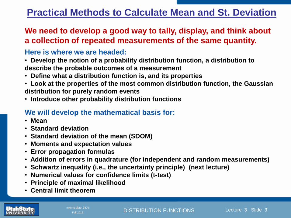
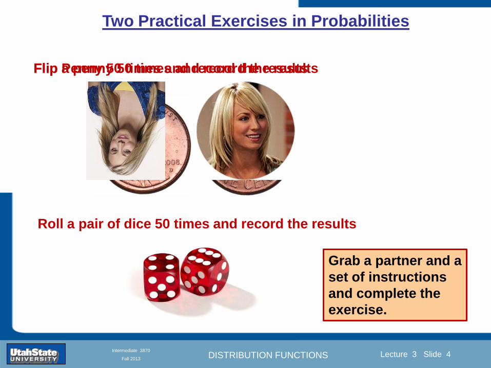
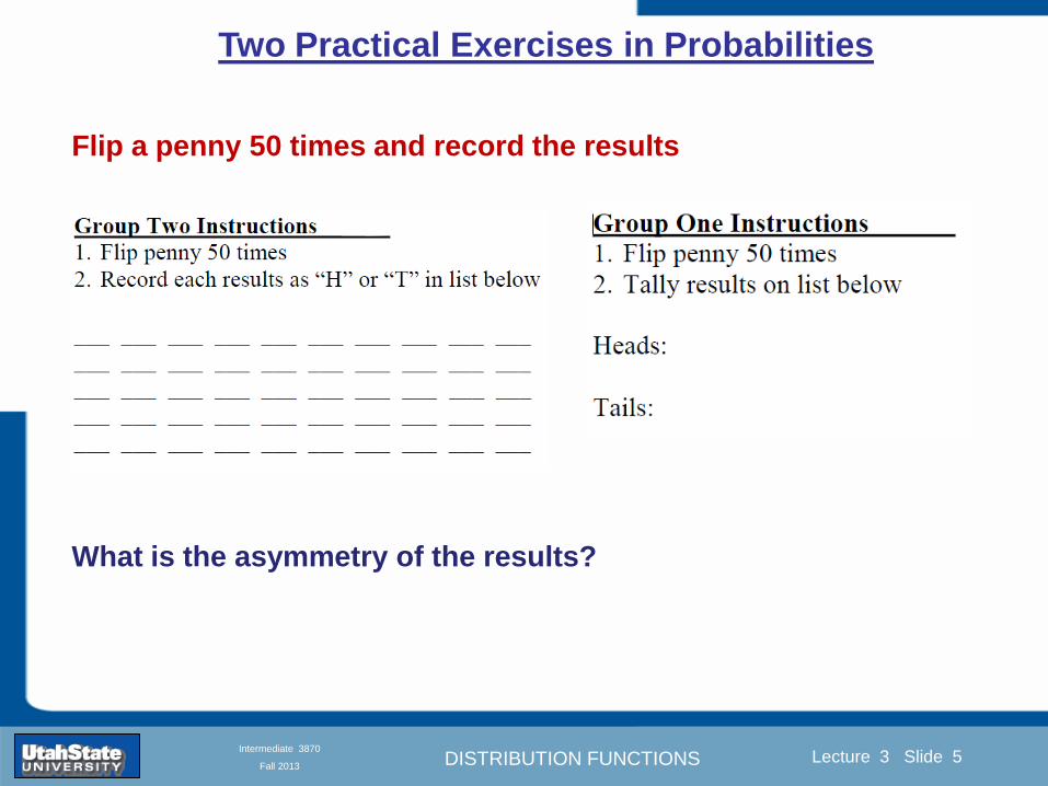
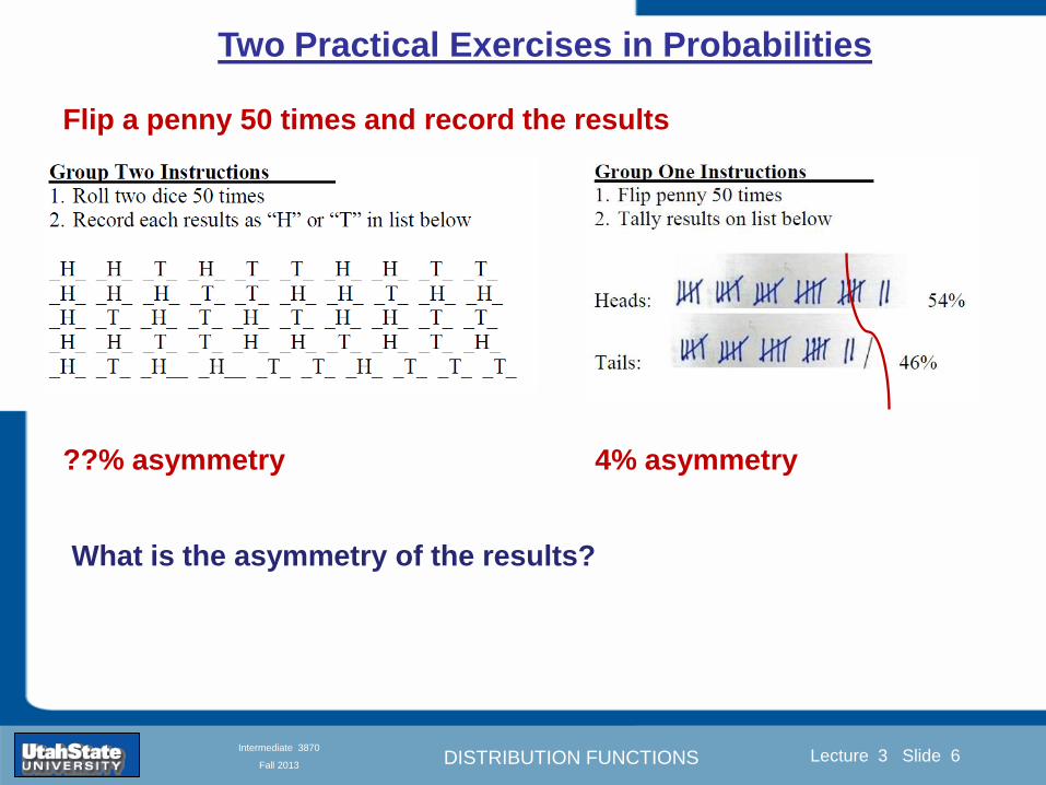
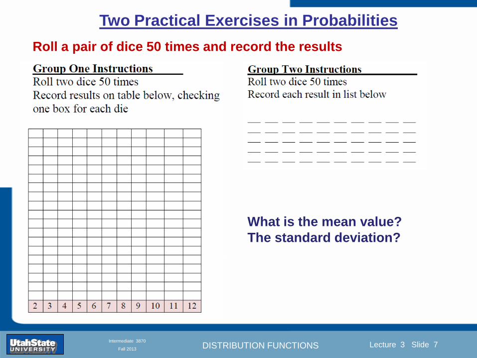
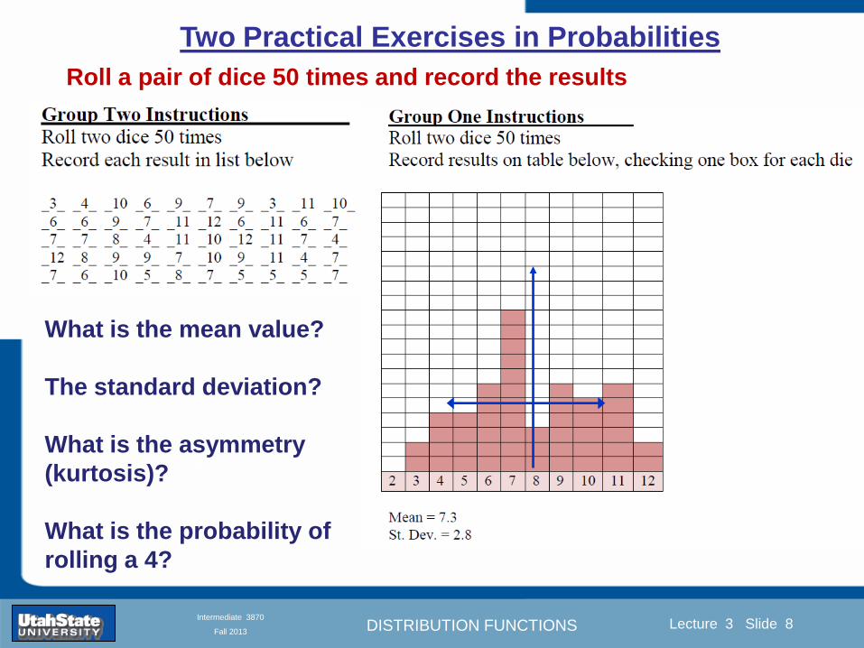
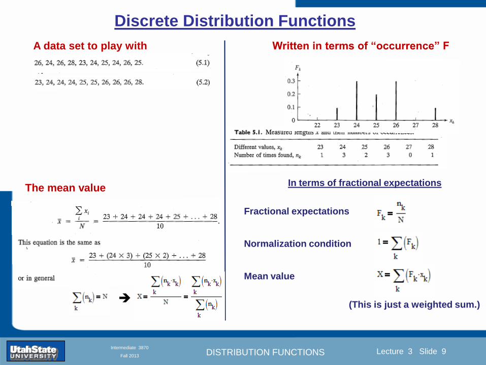
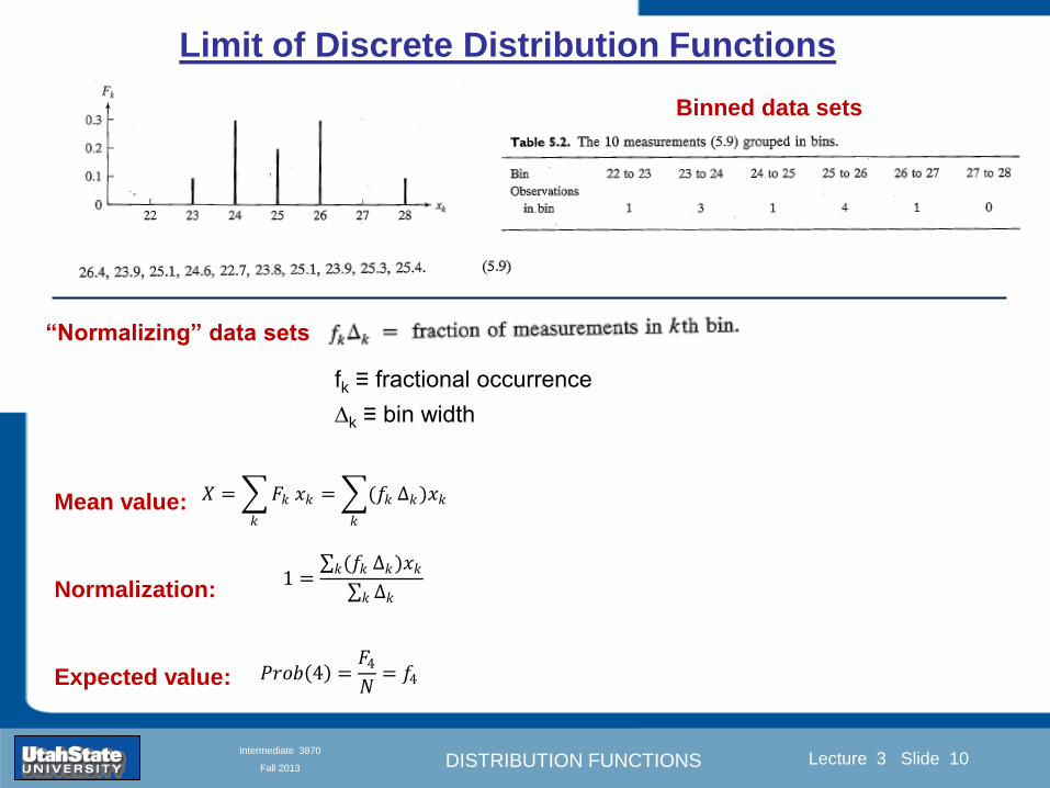
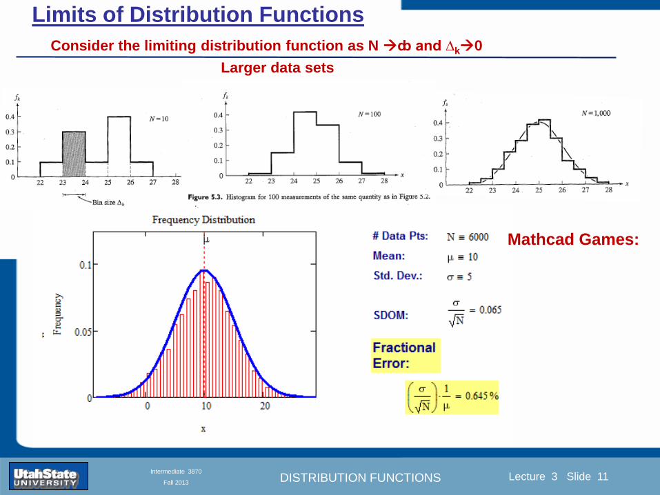
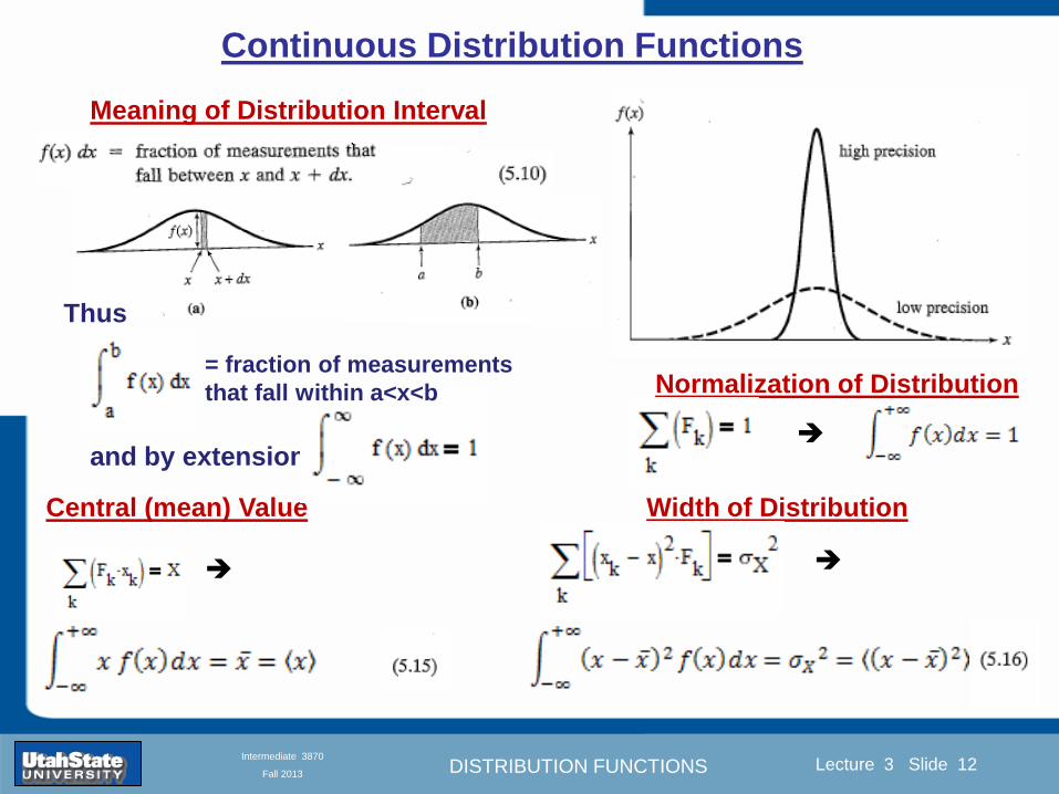
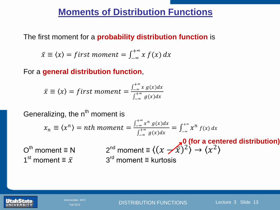
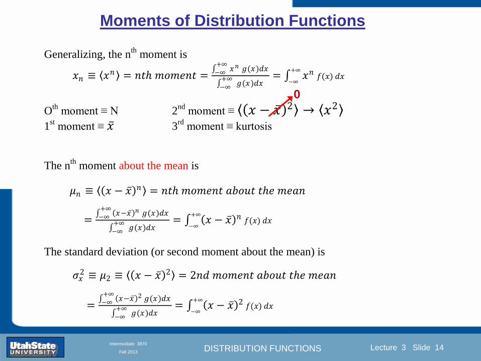
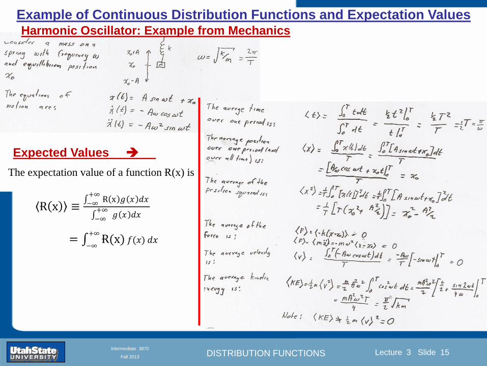
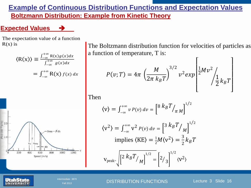
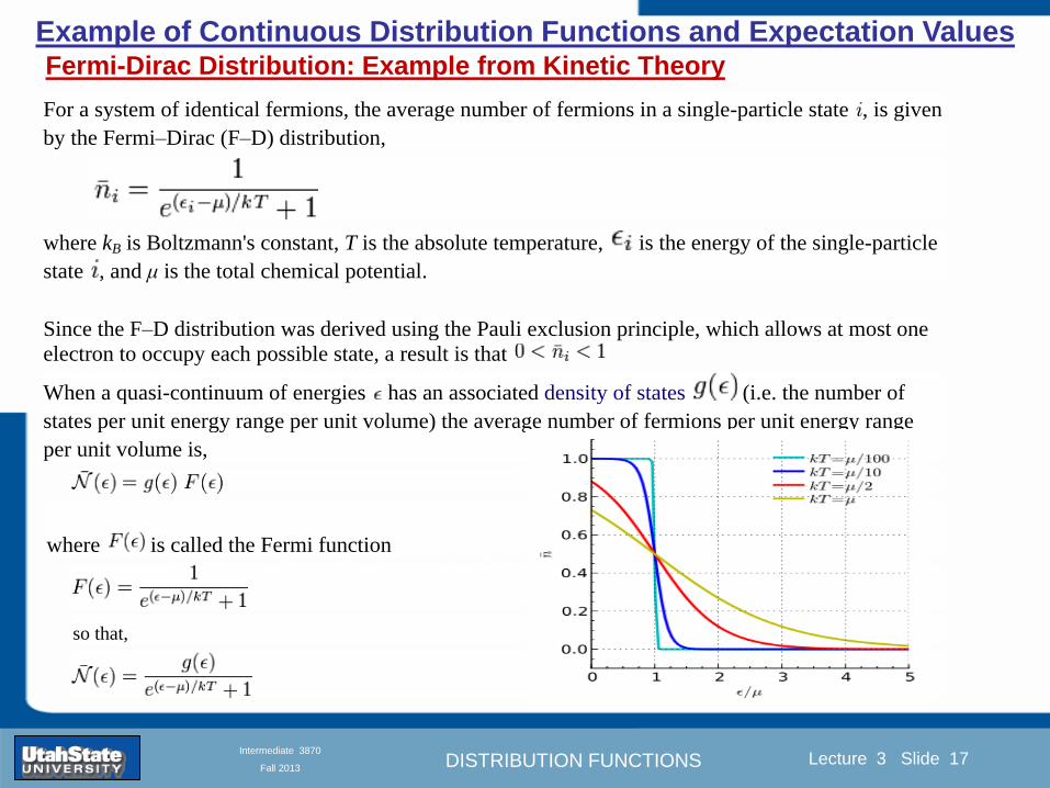
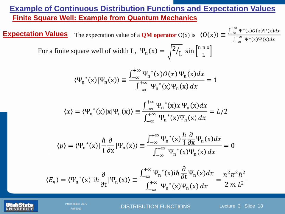
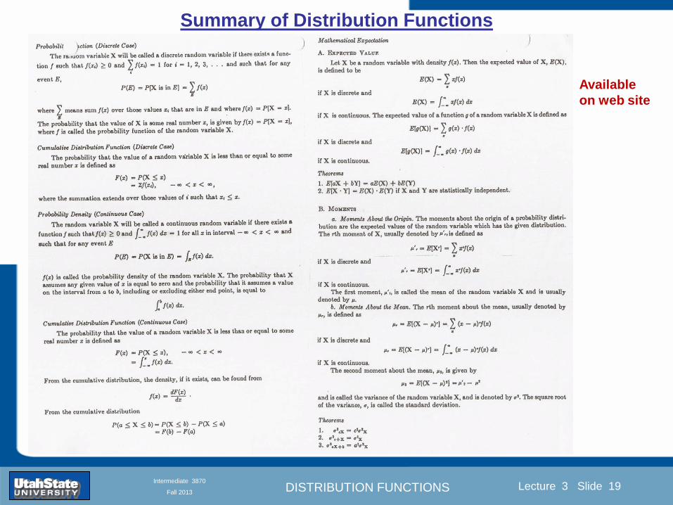
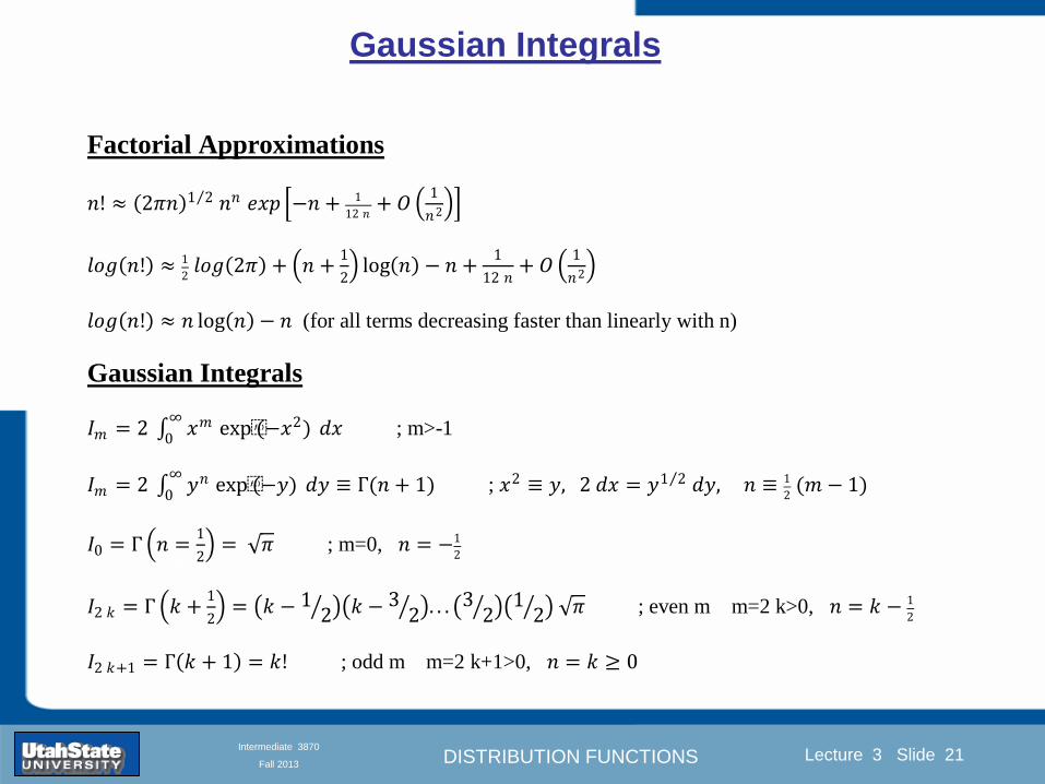
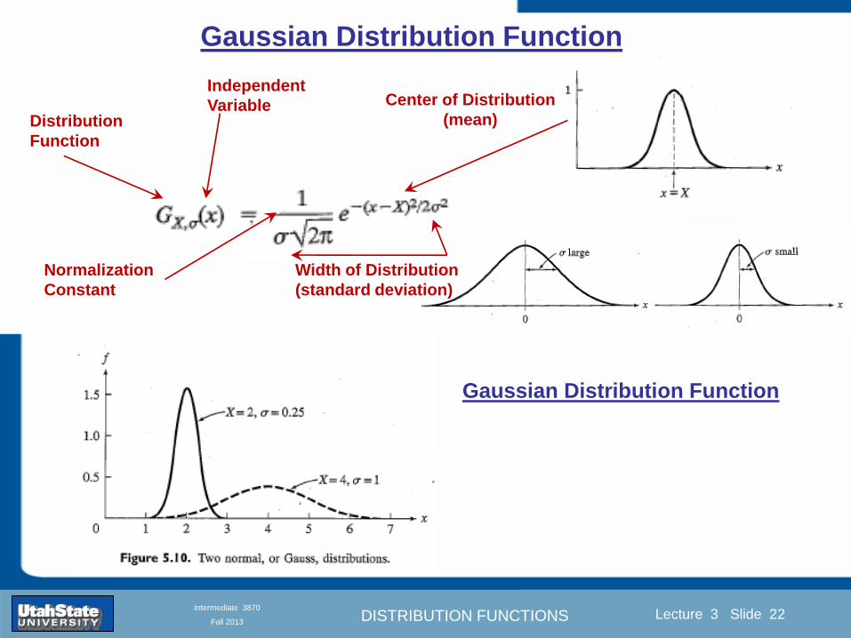
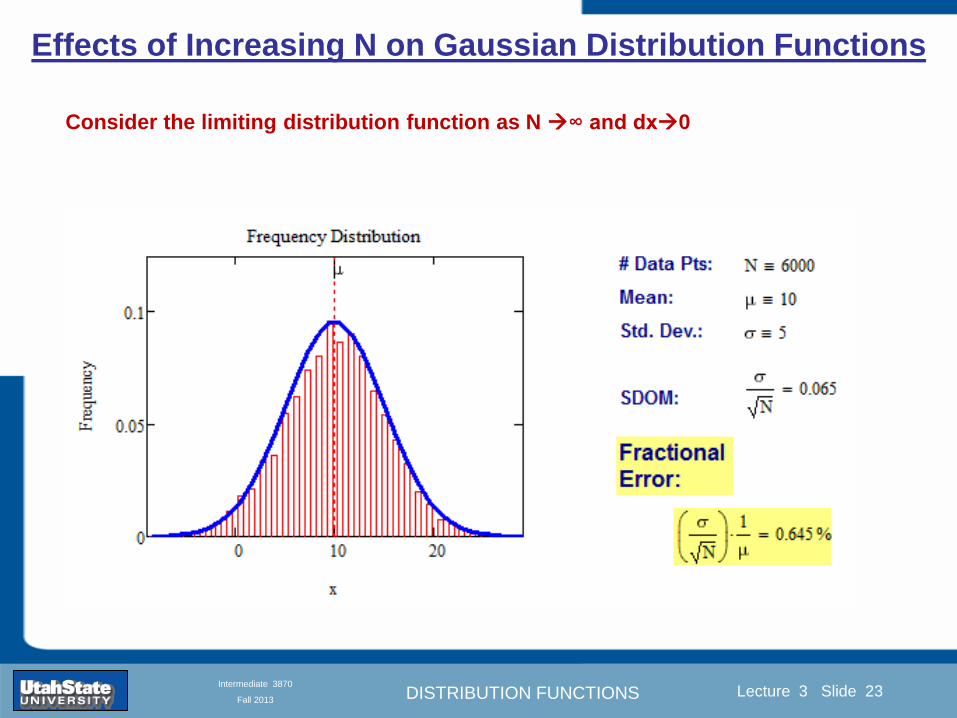
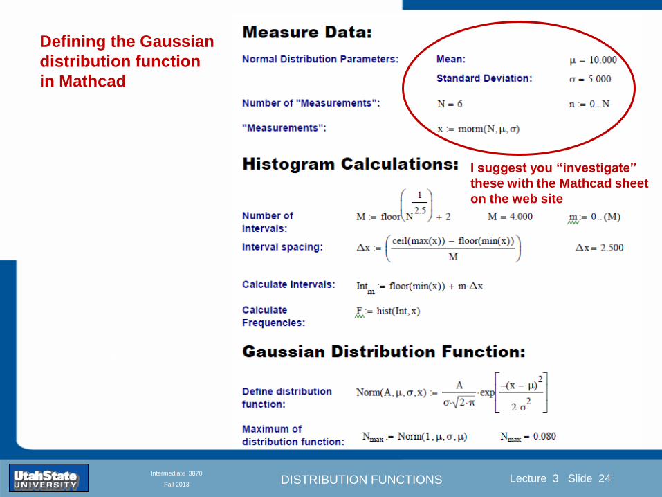
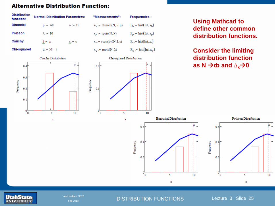
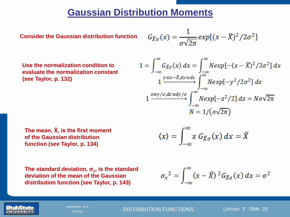
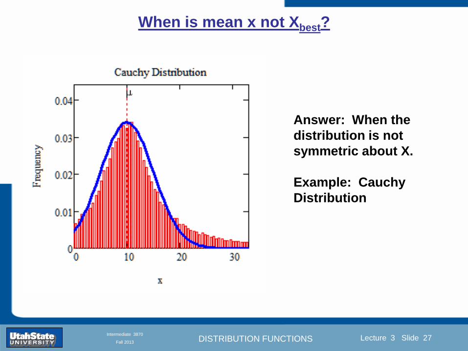
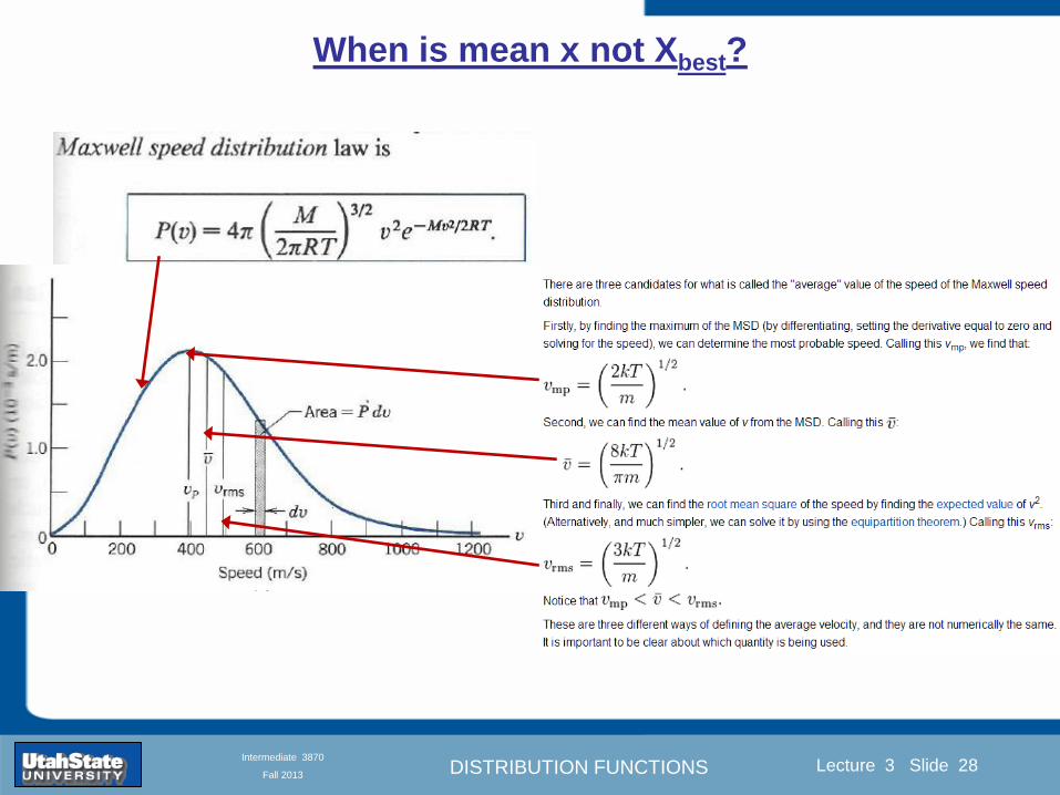
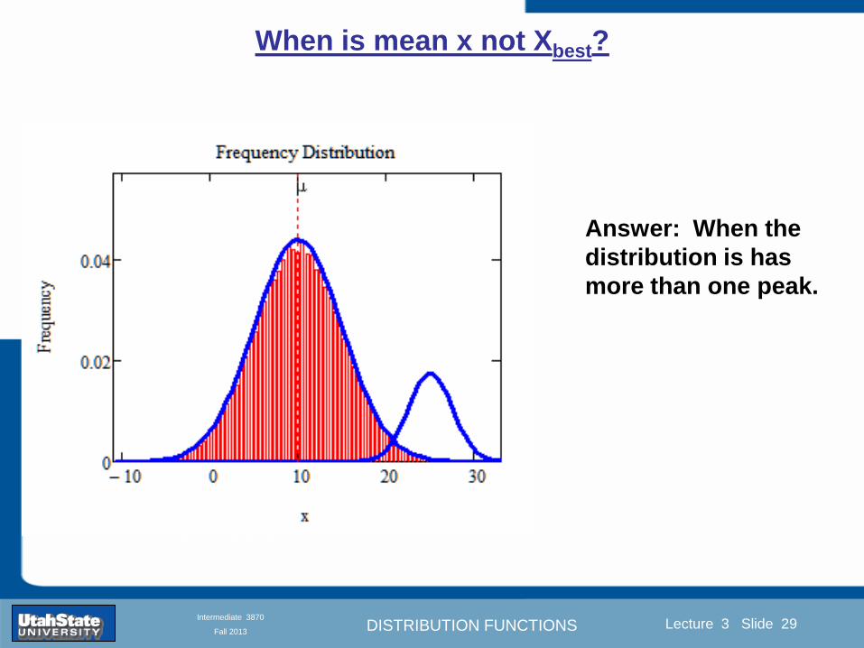
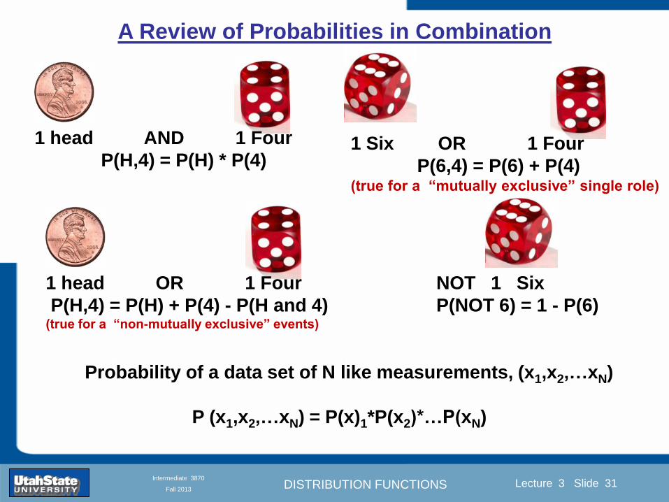
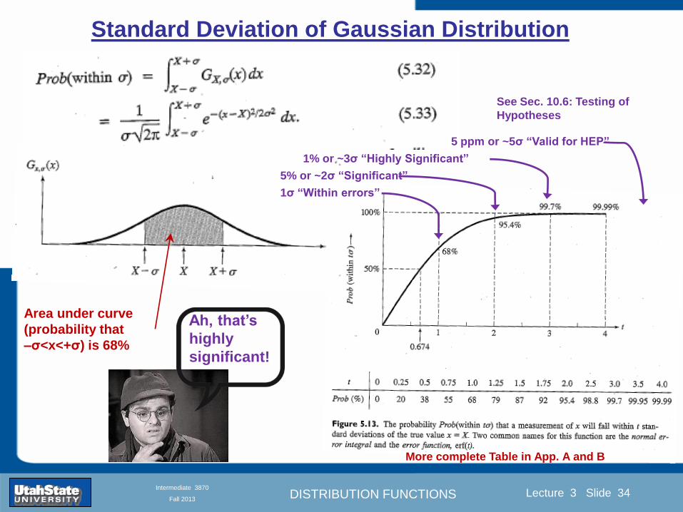
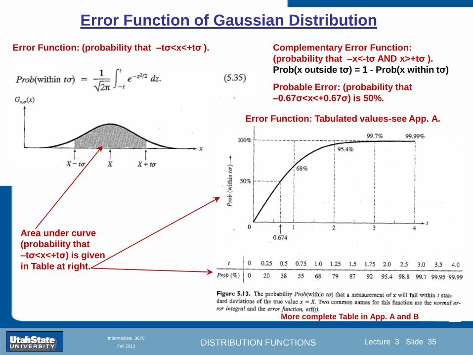
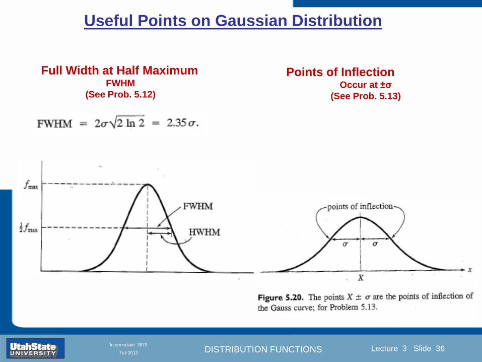
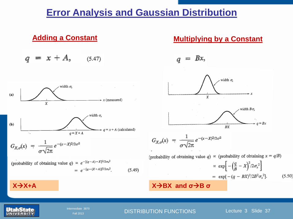
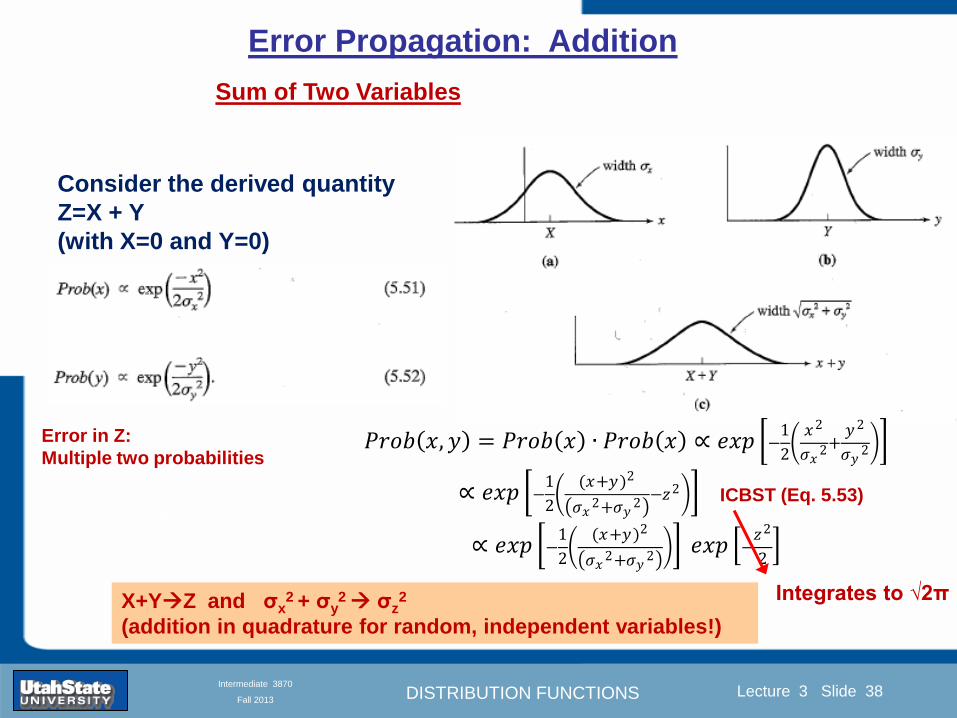
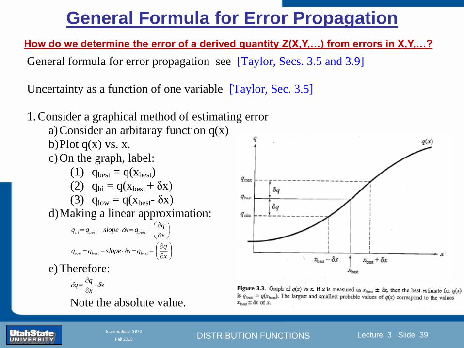
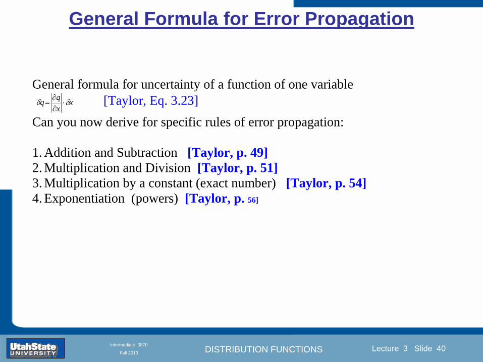
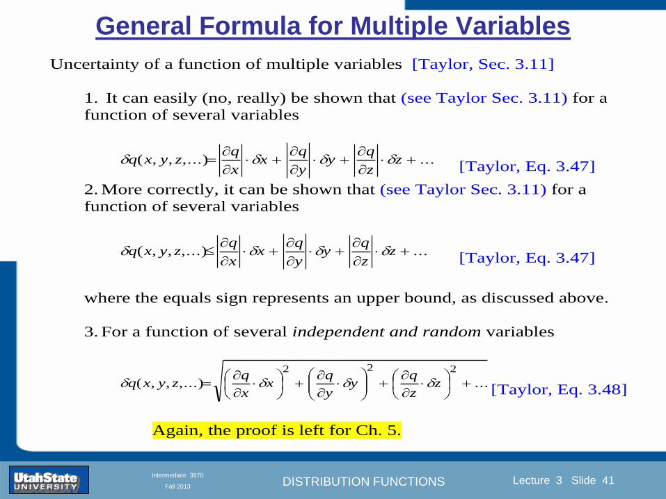
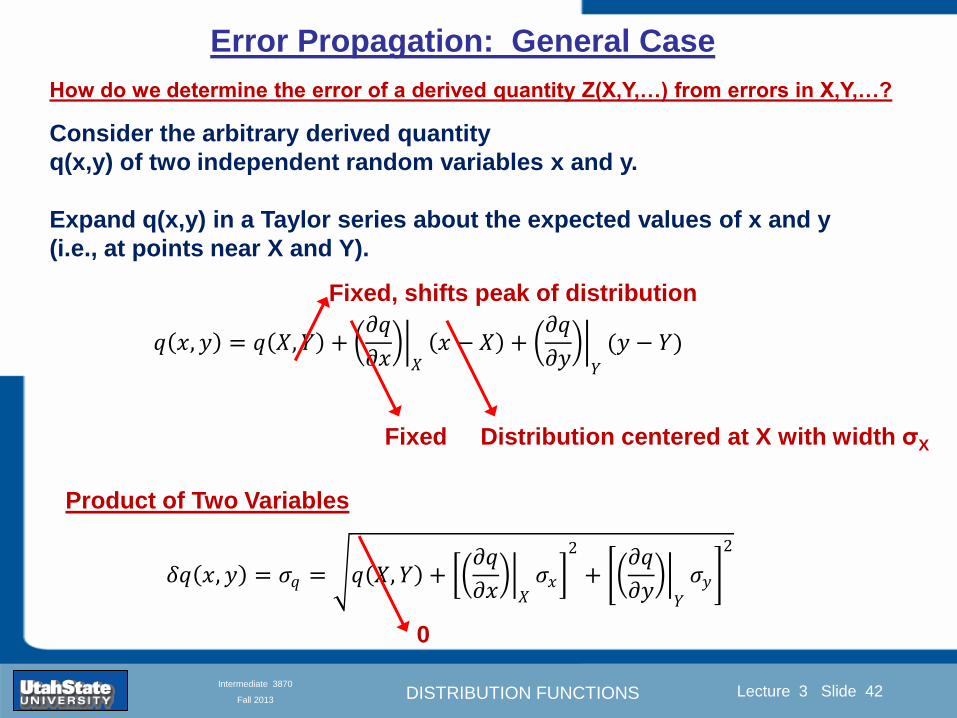
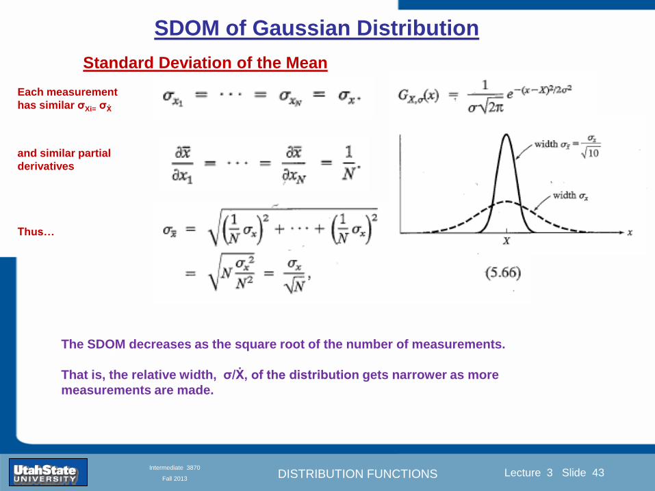
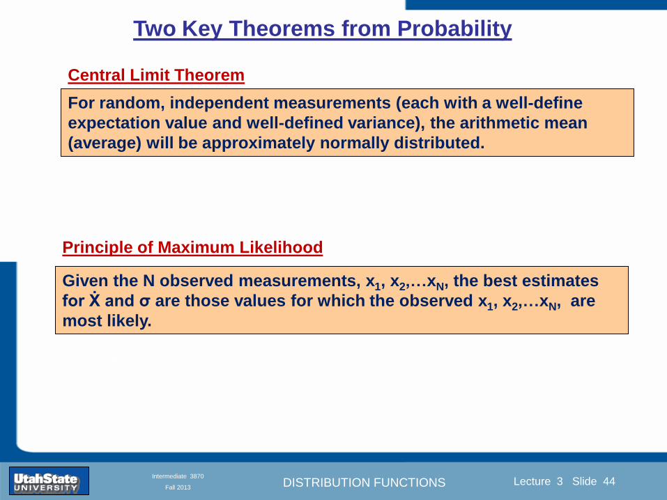
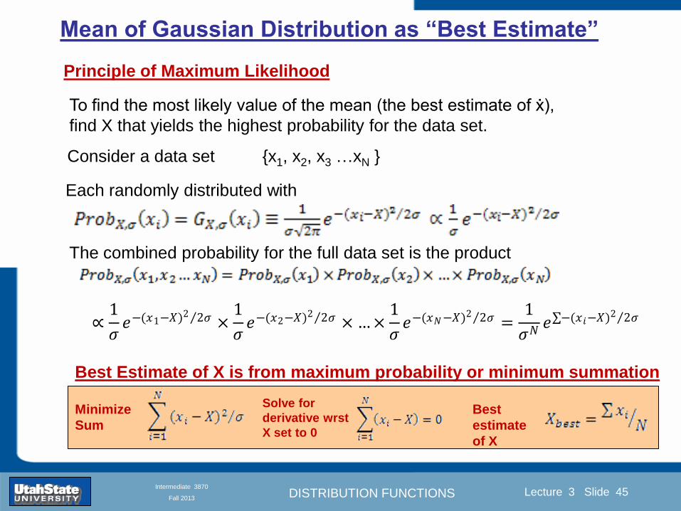
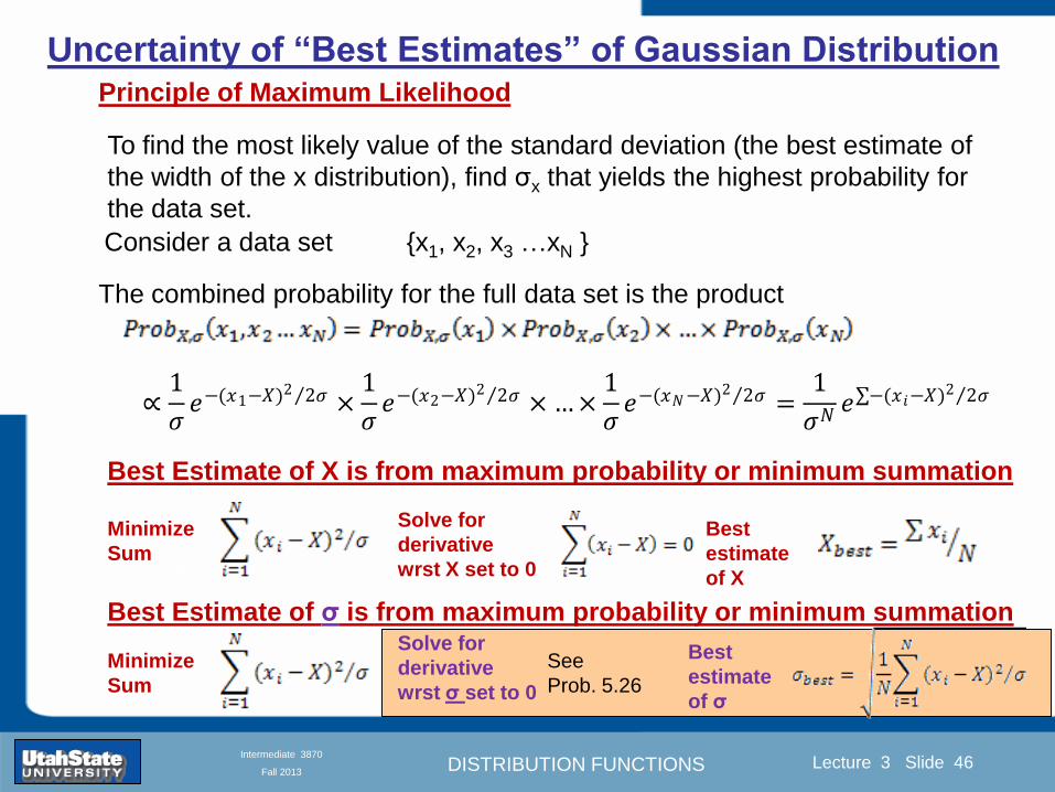
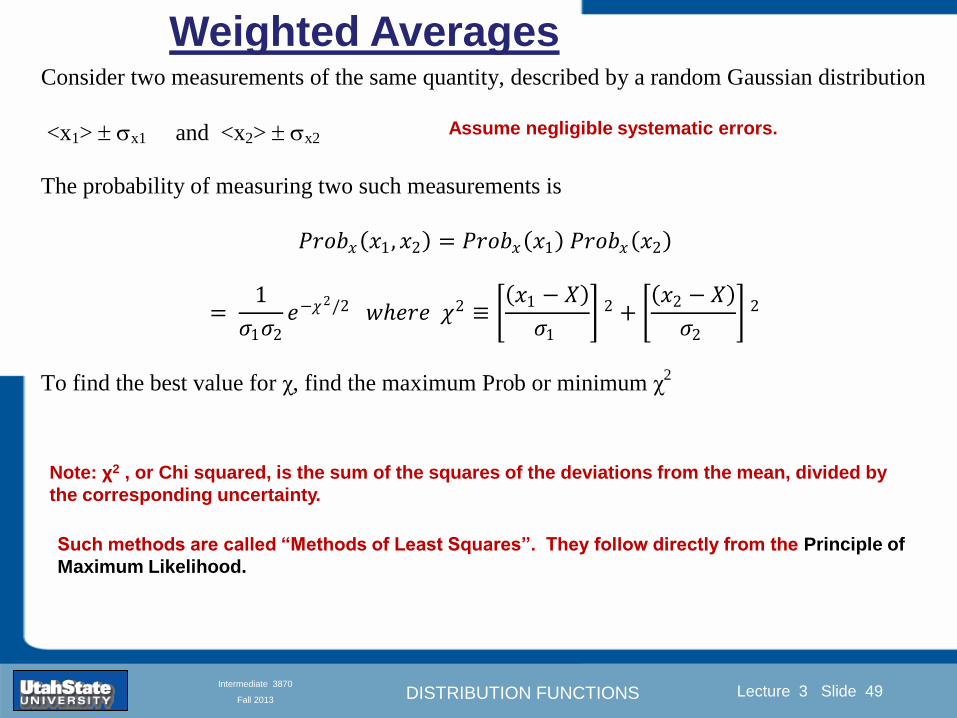
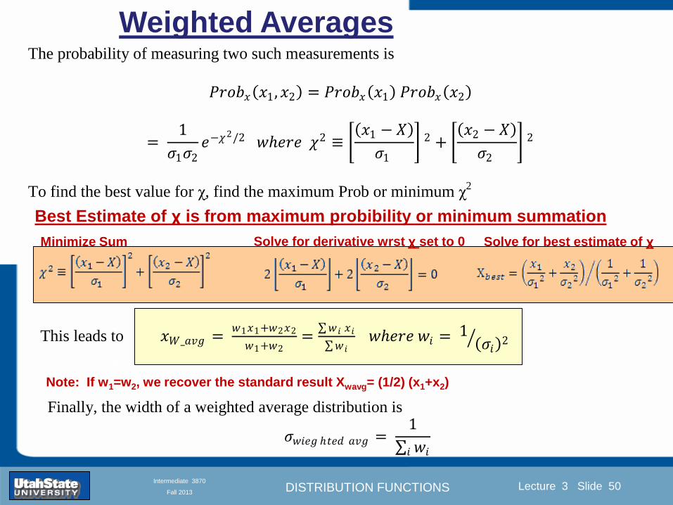
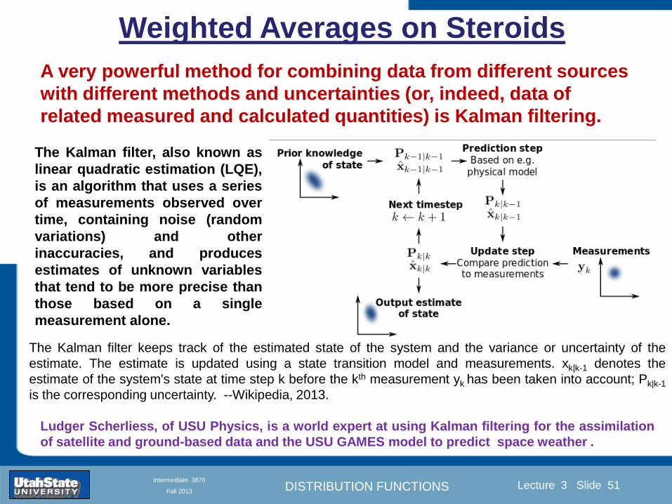
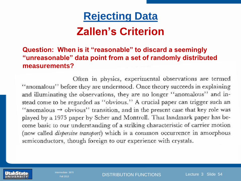
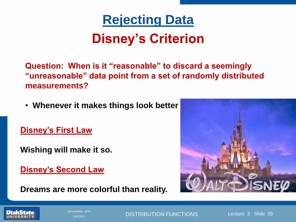
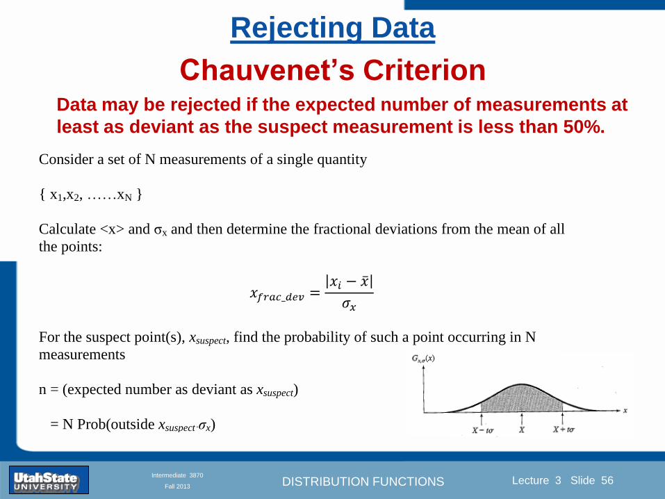
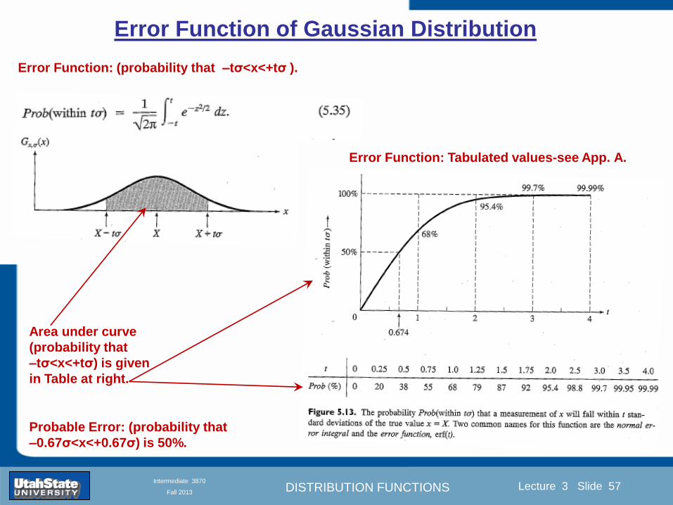
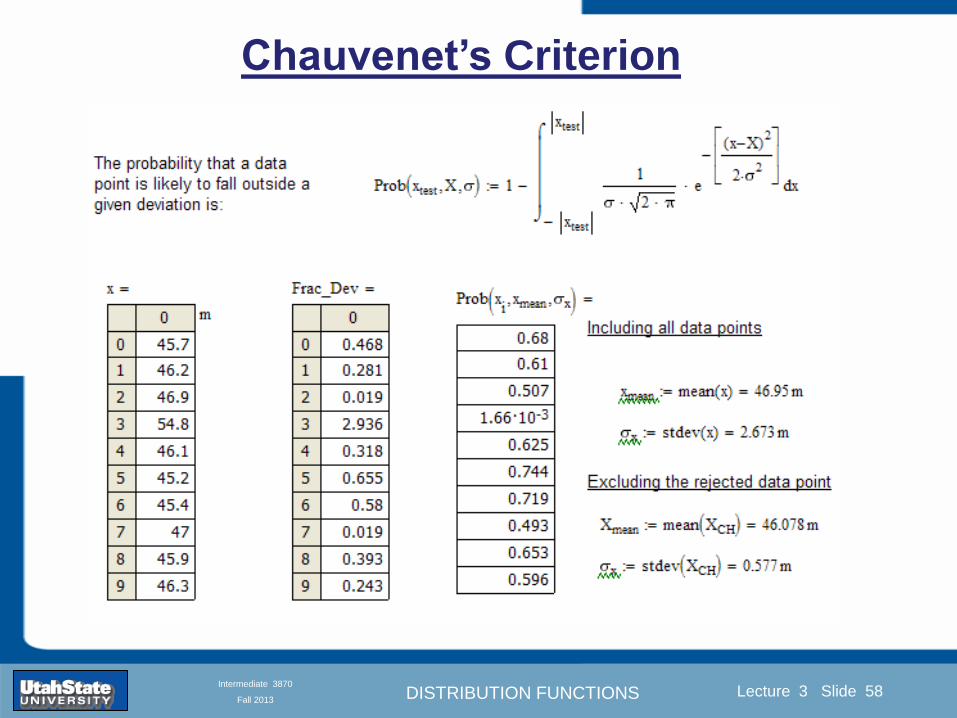
DISTRIBUTION FUNCTIONS

Introduction Section 0 Lecture 1 Slide 59

Lecture 3 Slide 59

INTRODUCTION TO Modern Physics PHYX 2710

Fall 2004

Intermediate 3870

Fall 2013

Chauvenetrsquos CriterionmdashExample 1

DISTRIBUTION FUNCTIONS

Introduction Section 0 Lecture 1 Slide 60

Lecture 3 Slide 60

INTRODUCTION TO Modern Physics PHYX 2710

Fall 2004

Intermediate 3870

Fall 2013

Chauvenetrsquos Details (1)

DISTRIBUTION FUNCTIONS

Introduction Section 0 Lecture 1 Slide 61

Lecture 3 Slide 61

INTRODUCTION TO Modern Physics PHYX 2710

Fall 2004

Intermediate 3870

Fall 2013

Chauvenetrsquos CriterionmdashDetails (2)

DISTRIBUTION FUNCTIONS

Introduction Section 0 Lecture 1 Slide 62

Lecture 3 Slide 62

INTRODUCTION TO Modern Physics PHYX 2710

Fall 2004

Intermediate 3870

Fall 2013

Chauvenetrsquos

Criterionmdash

Details (3)

DISTRIBUTION FUNCTIONS

Introduction Section 0 Lecture 1 Slide 63

Lecture 3 Slide 63

INTRODUCTION TO Modern Physics PHYX 2710

Fall 2004

Intermediate 3870

Fall 2013

Chauvenetrsquos

Criterionmdash

Example 2

DISTRIBUTION FUNCTIONS

Introduction Section 0 Lecture 1 Slide 64

Lecture 3 Slide 64

INTRODUCTION TO Modern Physics PHYX 2710

Fall 2004

Intermediate 3870

Fall 2013

Intermediate Lab PHYS 3870

Summary of Probability Theory

DISTRIBUTION FUNCTIONS

Introduction Section 0 Lecture 1 Slide 65

Lecture 3 Slide 65

INTRODUCTION TO Modern Physics PHYX 2710

Fall 2004

Intermediate 3870

Fall 2013

Summary of

Probability

Theory-I

DISTRIBUTION FUNCTIONS

Introduction Section 0 Lecture 1 Slide 66

Lecture 3 Slide 66

INTRODUCTION TO Modern Physics PHYX 2710

Fall 2004

Intermediate 3870

Fall 2013

Summary of

Probability

Theory-II

DISTRIBUTION FUNCTIONS

Introduction Section 0 Lecture 1 Slide 67

Lecture 3 Slide 67

INTRODUCTION TO Modern Physics PHYX 2710

Fall 2004

Intermediate 3870

Fall 2013

Summary of Probability Theory-III

DISTRIBUTION FUNCTIONS

Introduction Section 0 Lecture 1 Slide 68

Lecture 3 Slide 68

INTRODUCTION TO Modern Physics PHYX 2710

Fall 2004

Intermediate 3870

Fall 2013

Summary of Probability Theory-IV

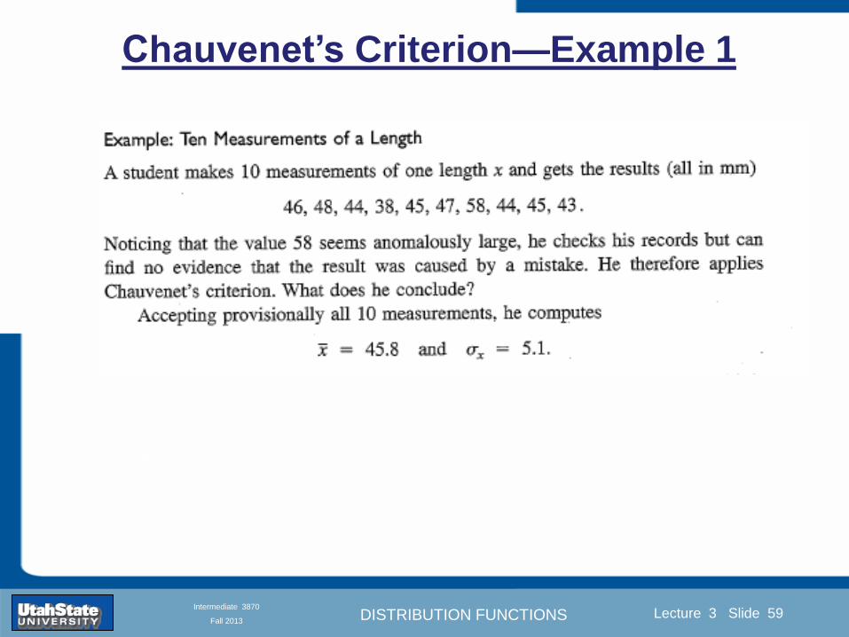
DISTRIBUTION FUNCTIONS

Introduction Section 0 Lecture 1 Slide 60

Lecture 3 Slide 60

INTRODUCTION TO Modern Physics PHYX 2710

Fall 2004

Intermediate 3870

Fall 2013

Chauvenetrsquos Details (1)

DISTRIBUTION FUNCTIONS

Introduction Section 0 Lecture 1 Slide 61

Lecture 3 Slide 61

INTRODUCTION TO Modern Physics PHYX 2710

Fall 2004

Intermediate 3870

Fall 2013

Chauvenetrsquos CriterionmdashDetails (2)

DISTRIBUTION FUNCTIONS

Introduction Section 0 Lecture 1 Slide 62

Lecture 3 Slide 62

INTRODUCTION TO Modern Physics PHYX 2710

Fall 2004

Intermediate 3870

Fall 2013

Chauvenetrsquos

Criterionmdash

Details (3)

DISTRIBUTION FUNCTIONS

Introduction Section 0 Lecture 1 Slide 63

Lecture 3 Slide 63

INTRODUCTION TO Modern Physics PHYX 2710

Fall 2004

Intermediate 3870

Fall 2013

Chauvenetrsquos

Criterionmdash

Example 2

DISTRIBUTION FUNCTIONS

Introduction Section 0 Lecture 1 Slide 64

Lecture 3 Slide 64

INTRODUCTION TO Modern Physics PHYX 2710

Fall 2004

Intermediate 3870

Fall 2013

Intermediate Lab PHYS 3870

Summary of Probability Theory

DISTRIBUTION FUNCTIONS

Introduction Section 0 Lecture 1 Slide 65

Lecture 3 Slide 65

INTRODUCTION TO Modern Physics PHYX 2710

Fall 2004

Intermediate 3870

Fall 2013

Summary of

Probability

Theory-I

DISTRIBUTION FUNCTIONS

Introduction Section 0 Lecture 1 Slide 66

Lecture 3 Slide 66

INTRODUCTION TO Modern Physics PHYX 2710

Fall 2004

Intermediate 3870

Fall 2013

Summary of

Probability

Theory-II

DISTRIBUTION FUNCTIONS

Introduction Section 0 Lecture 1 Slide 67

Lecture 3 Slide 67

INTRODUCTION TO Modern Physics PHYX 2710

Fall 2004

Intermediate 3870

Fall 2013

Summary of Probability Theory-III

DISTRIBUTION FUNCTIONS

Introduction Section 0 Lecture 1 Slide 68

Lecture 3 Slide 68

INTRODUCTION TO Modern Physics PHYX 2710

Fall 2004

Intermediate 3870

Fall 2013

Summary of Probability Theory-IV

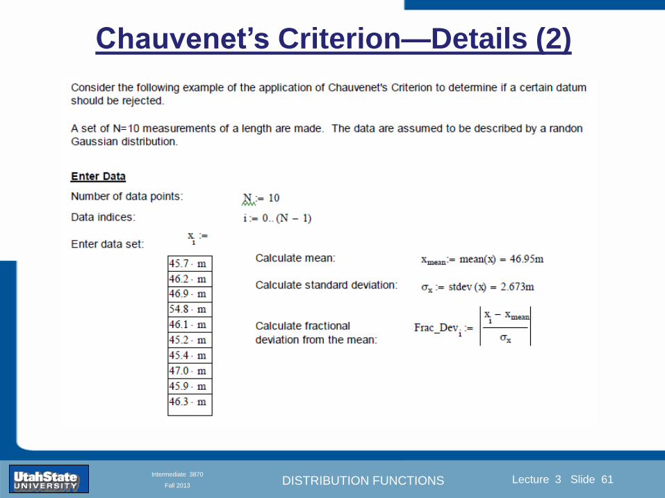
DISTRIBUTION FUNCTIONS

Introduction Section 0 Lecture 1 Slide 61

Lecture 3 Slide 61

INTRODUCTION TO Modern Physics PHYX 2710

Fall 2004

Intermediate 3870

Fall 2013

Chauvenetrsquos CriterionmdashDetails (2)

DISTRIBUTION FUNCTIONS

Introduction Section 0 Lecture 1 Slide 62

Lecture 3 Slide 62

INTRODUCTION TO Modern Physics PHYX 2710

Fall 2004

Intermediate 3870

Fall 2013

Chauvenetrsquos

Criterionmdash

Details (3)

DISTRIBUTION FUNCTIONS

Introduction Section 0 Lecture 1 Slide 63

Lecture 3 Slide 63

INTRODUCTION TO Modern Physics PHYX 2710

Fall 2004

Intermediate 3870

Fall 2013

Chauvenetrsquos

Criterionmdash

Example 2

DISTRIBUTION FUNCTIONS

Introduction Section 0 Lecture 1 Slide 64

Lecture 3 Slide 64

INTRODUCTION TO Modern Physics PHYX 2710

Fall 2004

Intermediate 3870

Fall 2013

Intermediate Lab PHYS 3870

Summary of Probability Theory

DISTRIBUTION FUNCTIONS

Introduction Section 0 Lecture 1 Slide 65

Lecture 3 Slide 65

INTRODUCTION TO Modern Physics PHYX 2710

Fall 2004

Intermediate 3870

Fall 2013

Summary of

Probability

Theory-I

DISTRIBUTION FUNCTIONS

Introduction Section 0 Lecture 1 Slide 66

Lecture 3 Slide 66

INTRODUCTION TO Modern Physics PHYX 2710

Fall 2004

Intermediate 3870

Fall 2013

Summary of

Probability

Theory-II

DISTRIBUTION FUNCTIONS

Introduction Section 0 Lecture 1 Slide 67

Lecture 3 Slide 67

INTRODUCTION TO Modern Physics PHYX 2710

Fall 2004

Intermediate 3870

Fall 2013

Summary of Probability Theory-III

DISTRIBUTION FUNCTIONS

Introduction Section 0 Lecture 1 Slide 68

Lecture 3 Slide 68

INTRODUCTION TO Modern Physics PHYX 2710

Fall 2004

Intermediate 3870

Fall 2013

Summary of Probability Theory-IV

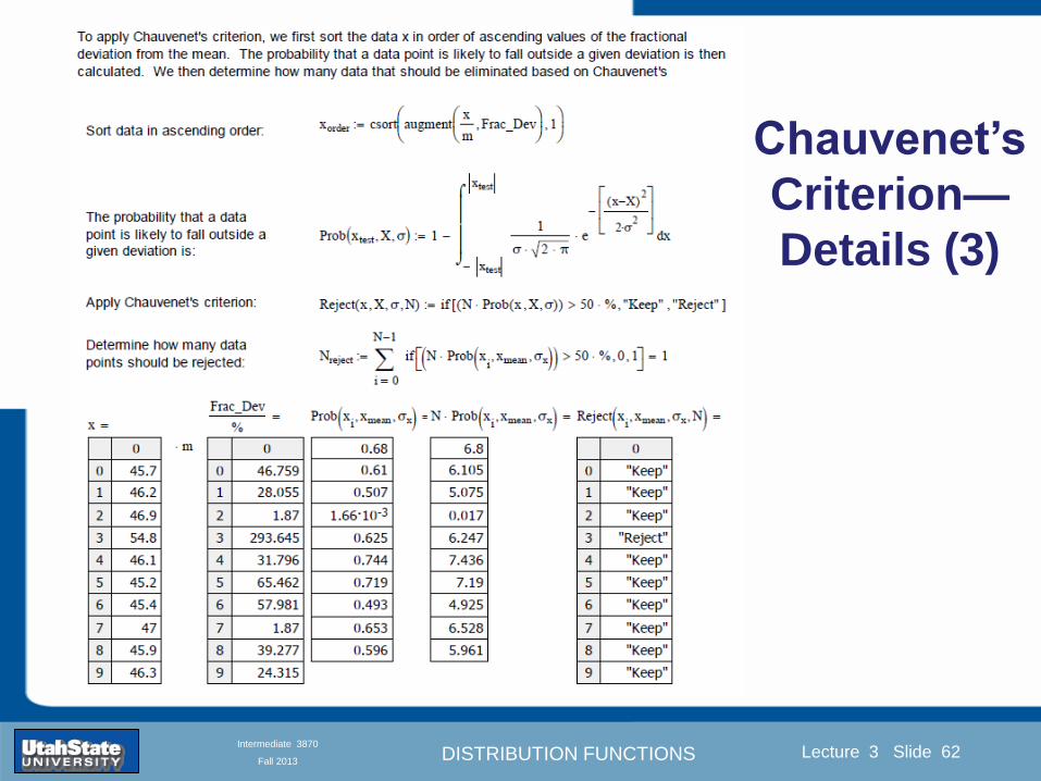
DISTRIBUTION FUNCTIONS

Introduction Section 0 Lecture 1 Slide 62

Lecture 3 Slide 62

INTRODUCTION TO Modern Physics PHYX 2710

Fall 2004

Intermediate 3870

Fall 2013

Chauvenetrsquos

Criterionmdash

Details (3)

DISTRIBUTION FUNCTIONS

Introduction Section 0 Lecture 1 Slide 63

Lecture 3 Slide 63

INTRODUCTION TO Modern Physics PHYX 2710

Fall 2004

Intermediate 3870

Fall 2013

Chauvenetrsquos

Criterionmdash

Example 2

DISTRIBUTION FUNCTIONS

Introduction Section 0 Lecture 1 Slide 64

Lecture 3 Slide 64

INTRODUCTION TO Modern Physics PHYX 2710

Fall 2004

Intermediate 3870

Fall 2013

Intermediate Lab PHYS 3870

Summary of Probability Theory

DISTRIBUTION FUNCTIONS

Introduction Section 0 Lecture 1 Slide 65

Lecture 3 Slide 65

INTRODUCTION TO Modern Physics PHYX 2710

Fall 2004

Intermediate 3870

Fall 2013

Summary of

Probability

Theory-I

DISTRIBUTION FUNCTIONS

Introduction Section 0 Lecture 1 Slide 66

Lecture 3 Slide 66

INTRODUCTION TO Modern Physics PHYX 2710

Fall 2004

Intermediate 3870

Fall 2013

Summary of

Probability

Theory-II

DISTRIBUTION FUNCTIONS

Introduction Section 0 Lecture 1 Slide 67

Lecture 3 Slide 67

INTRODUCTION TO Modern Physics PHYX 2710

Fall 2004

Intermediate 3870

Fall 2013

Summary of Probability Theory-III

DISTRIBUTION FUNCTIONS

Introduction Section 0 Lecture 1 Slide 68

Lecture 3 Slide 68

INTRODUCTION TO Modern Physics PHYX 2710

Fall 2004

Intermediate 3870

Fall 2013

Summary of Probability Theory-IV

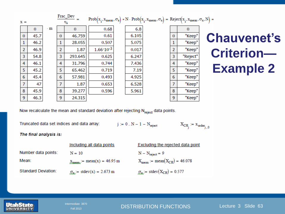
DISTRIBUTION FUNCTIONS

Introduction Section 0 Lecture 1 Slide 63

Lecture 3 Slide 63

INTRODUCTION TO Modern Physics PHYX 2710

Fall 2004

Intermediate 3870

Fall 2013

Chauvenetrsquos

Criterionmdash

Example 2

DISTRIBUTION FUNCTIONS

Introduction Section 0 Lecture 1 Slide 64

Lecture 3 Slide 64

INTRODUCTION TO Modern Physics PHYX 2710

Fall 2004

Intermediate 3870

Fall 2013

Intermediate Lab PHYS 3870

Summary of Probability Theory

DISTRIBUTION FUNCTIONS

Introduction Section 0 Lecture 1 Slide 65

Lecture 3 Slide 65

INTRODUCTION TO Modern Physics PHYX 2710

Fall 2004

Intermediate 3870

Fall 2013

Summary of

Probability

Theory-I

DISTRIBUTION FUNCTIONS

Introduction Section 0 Lecture 1 Slide 66

Lecture 3 Slide 66

INTRODUCTION TO Modern Physics PHYX 2710

Fall 2004

Intermediate 3870

Fall 2013

Summary of

Probability

Theory-II

DISTRIBUTION FUNCTIONS

Introduction Section 0 Lecture 1 Slide 67

Lecture 3 Slide 67

INTRODUCTION TO Modern Physics PHYX 2710

Fall 2004

Intermediate 3870

Fall 2013

Summary of Probability Theory-III

DISTRIBUTION FUNCTIONS

Introduction Section 0 Lecture 1 Slide 68

Lecture 3 Slide 68

INTRODUCTION TO Modern Physics PHYX 2710

Fall 2004

Intermediate 3870

Fall 2013

Summary of Probability Theory-IV

DISTRIBUTION FUNCTIONS

Introduction Section 0 Lecture 1 Slide 64

Lecture 3 Slide 64

INTRODUCTION TO Modern Physics PHYX 2710

Fall 2004

Intermediate 3870

Fall 2013

Intermediate Lab PHYS 3870

Summary of Probability Theory

DISTRIBUTION FUNCTIONS

Introduction Section 0 Lecture 1 Slide 65

Lecture 3 Slide 65

INTRODUCTION TO Modern Physics PHYX 2710

Fall 2004

Intermediate 3870

Fall 2013

Summary of

Probability

Theory-I

DISTRIBUTION FUNCTIONS

Introduction Section 0 Lecture 1 Slide 66

Lecture 3 Slide 66

INTRODUCTION TO Modern Physics PHYX 2710

Fall 2004

Intermediate 3870

Fall 2013

Summary of

Probability

Theory-II

DISTRIBUTION FUNCTIONS

Introduction Section 0 Lecture 1 Slide 67

Lecture 3 Slide 67

INTRODUCTION TO Modern Physics PHYX 2710

Fall 2004

Intermediate 3870

Fall 2013

Summary of Probability Theory-III

DISTRIBUTION FUNCTIONS

Introduction Section 0 Lecture 1 Slide 68

Lecture 3 Slide 68

INTRODUCTION TO Modern Physics PHYX 2710

Fall 2004

Intermediate 3870

Fall 2013

Summary of Probability Theory-IV

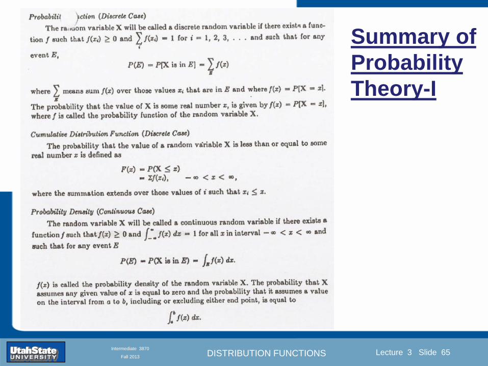
DISTRIBUTION FUNCTIONS

Introduction Section 0 Lecture 1 Slide 65

Lecture 3 Slide 65

INTRODUCTION TO Modern Physics PHYX 2710

Fall 2004

Intermediate 3870

Fall 2013

Summary of

Probability

Theory-I

DISTRIBUTION FUNCTIONS

Introduction Section 0 Lecture 1 Slide 66

Lecture 3 Slide 66

INTRODUCTION TO Modern Physics PHYX 2710

Fall 2004

Intermediate 3870

Fall 2013

Summary of

Probability

Theory-II

DISTRIBUTION FUNCTIONS

Introduction Section 0 Lecture 1 Slide 67

Lecture 3 Slide 67

INTRODUCTION TO Modern Physics PHYX 2710

Fall 2004

Intermediate 3870

Fall 2013

Summary of Probability Theory-III

DISTRIBUTION FUNCTIONS

Introduction Section 0 Lecture 1 Slide 68

Lecture 3 Slide 68

INTRODUCTION TO Modern Physics PHYX 2710

Fall 2004

Intermediate 3870

Fall 2013

Summary of Probability Theory-IV

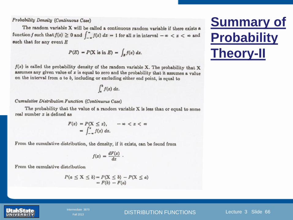
DISTRIBUTION FUNCTIONS

Introduction Section 0 Lecture 1 Slide 66

Lecture 3 Slide 66

INTRODUCTION TO Modern Physics PHYX 2710

Fall 2004

Intermediate 3870

Fall 2013

Summary of

Probability

Theory-II

DISTRIBUTION FUNCTIONS

Introduction Section 0 Lecture 1 Slide 67

Lecture 3 Slide 67

INTRODUCTION TO Modern Physics PHYX 2710

Fall 2004

Intermediate 3870

Fall 2013

Summary of Probability Theory-III

DISTRIBUTION FUNCTIONS

Introduction Section 0 Lecture 1 Slide 68

Lecture 3 Slide 68

INTRODUCTION TO Modern Physics PHYX 2710

Fall 2004

Intermediate 3870

Fall 2013

Summary of Probability Theory-IV

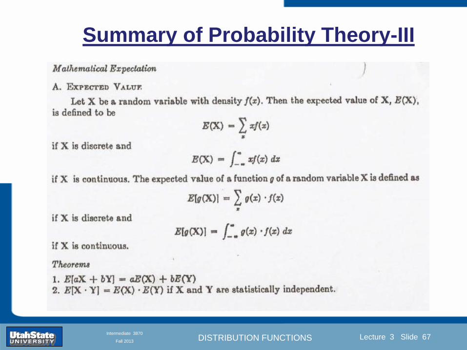
DISTRIBUTION FUNCTIONS

Introduction Section 0 Lecture 1 Slide 67

Lecture 3 Slide 67

INTRODUCTION TO Modern Physics PHYX 2710

Fall 2004

Intermediate 3870

Fall 2013

Summary of Probability Theory-III

DISTRIBUTION FUNCTIONS

Introduction Section 0 Lecture 1 Slide 68

Lecture 3 Slide 68

INTRODUCTION TO Modern Physics PHYX 2710

Fall 2004

Intermediate 3870

Fall 2013

Summary of Probability Theory-IV

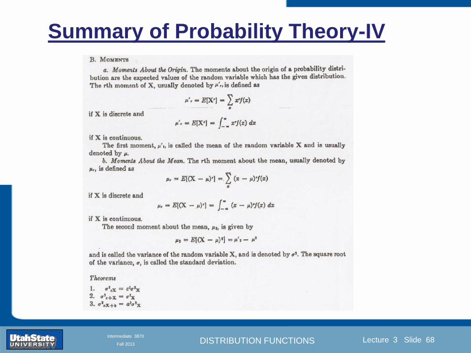
DISTRIBUTION FUNCTIONS

Introduction Section 0 Lecture 1 Slide 68

Lecture 3 Slide 68

INTRODUCTION TO Modern Physics PHYX 2710

Fall 2004

Intermediate 3870

Fall 2013

Summary of Probability Theory-IV