Introduction to Descriptive Statisticsweb.mit.edu/~17.871/www/2015/02descriptive_stats_2015.pdfKey...
99
Introduction to Descriptive Statistics 17.871 Spring 2015
Transcript of Introduction to Descriptive Statisticsweb.mit.edu/~17.871/www/2015/02descriptive_stats_2015.pdfKey...

Introduction to Descriptive Statistics
17.871
Spring 2015

Reasons for paying attention to data description
• Double-check data acquisition
• Data exploration
• Data explanation
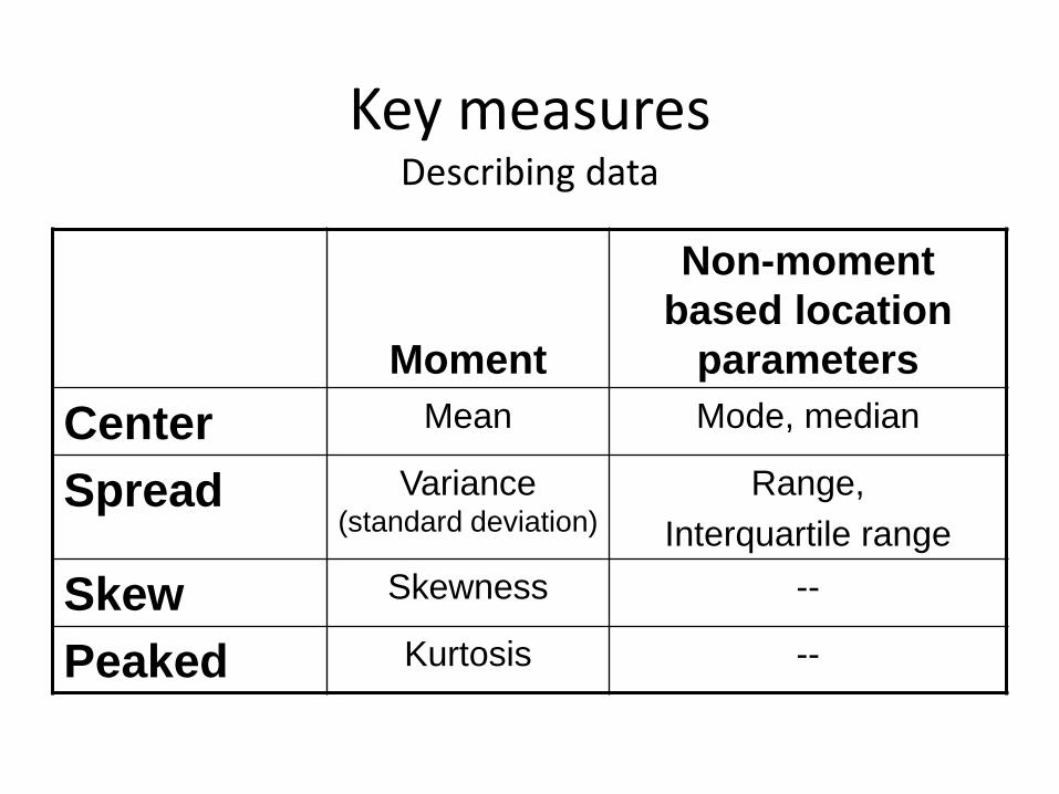
Key measures Describing data
Moment
Non-moment
based location
parameters
Center Mean Mode, median
Spread Variance (standard deviation)
Range,
Interquartile range
Skew Skewness --
Peaked Kurtosis --

Key distinction Population vs. Sample Notation
Population vs. Sample
Greeks Romans
μ, σ, β s, b

Mean
Xn
xn
i
i
1

Guess the Mean
Source: CCES
0.1
.2.3
.4
Den
sity
0strongly approve
somewhat approvesomewhat disapprove
strongly disapprove
institution approval - supreme court

Guess the Mean
Source: CCES
0.1
.2.3
.4
Den
sity
0 1 2 3 4institution approval - supreme court

Guess the Mean
Source: CCES
0.1
.2.3
.4
Den
sity
0 1 2 3 4institution approval - supreme court
2.8

Guess the Mean
0
.2
.4
.6
.8
Fra
ctio
n
0 10 20 30Number of medals

Guess the Mean
0
.2
.4
.6
.8
Fra
ctio
n
0 10 20 30Number of medals
3.3
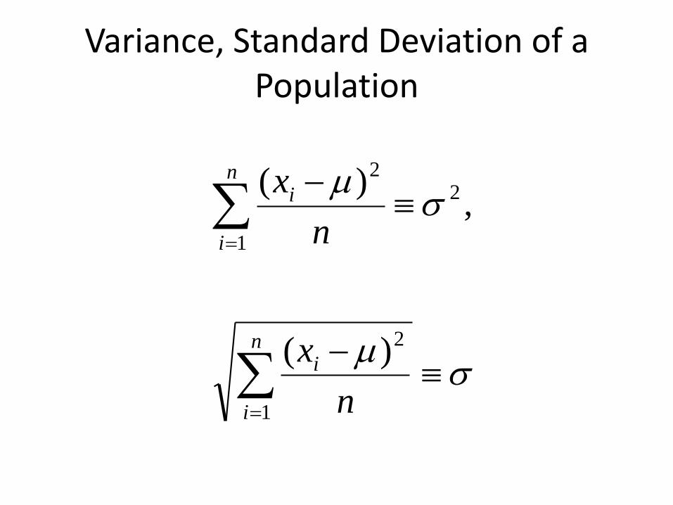
Variance, Standard Deviation of a Population
n
i
i
n
i
i
n
x
n
x
1
2
2
1
2
)(
,)(

Variance, S.D. of a Sample
sn
x
sn
x
n
i
i
n
i
i
1
2
2
1
2
1
)(
,1
)(
Degrees of freedom
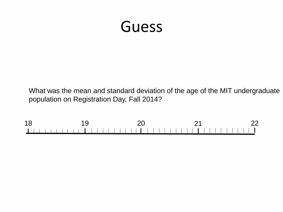
Guess
What was the mean and standard deviation of the age of the MIT undergraduate
population on Registration Day, Fall 2014?
18 19 20 21 22
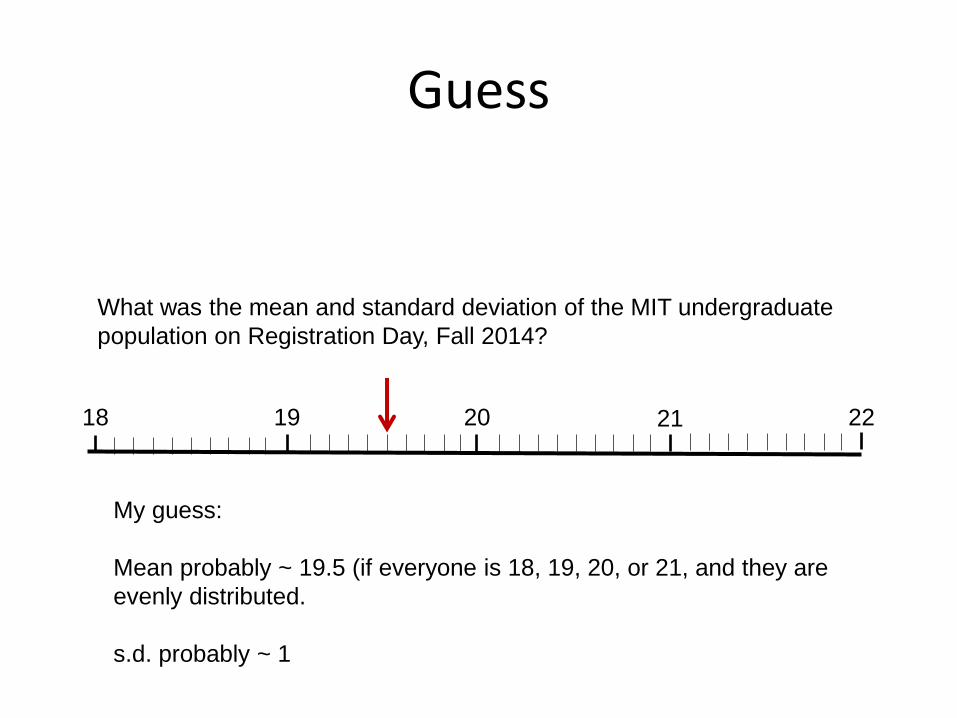
Guess
What was the mean and standard deviation of the MIT undergraduate
population on Registration Day, Fall 2014?
My guess:
Mean probably ~ 19.5 (if everyone is 18, 19, 20, or 21, and they are
evenly distributed.
s.d. probably ~ 1
18 19 20 21 22

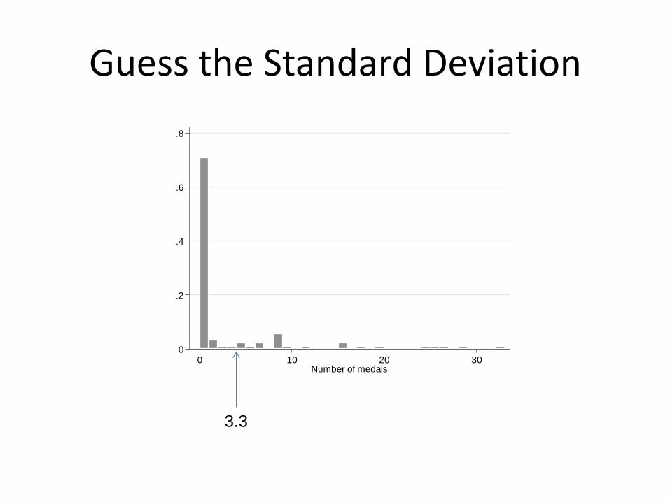
Guess the Standard Deviation
Source: CCES
0.1
.2.3
.4
Den
sity
0 1 2 3 4institution approval - supreme court

Guess the Standard Deviation
Source: CCES
0.1
.2.3
.4
Den
sity
0 1 2 3 4institution approval - supreme court
σ = 0.89
Guess the Standard Deviation
0
.2
.4
.6
.8
Fra
ctio
n
0 10 20 30Number of medals
3.3

Guess the Standard Deviation
0
.2
.4
.6
.8
Fra
ctio
n
0 10 20 30Number of medals
3.3 σ = 7.2

Binary data
)1()1(
1 timeof proportion1)(
2 xxsxxs
xXprobX
xx

Example of this, using the most recent Gallup approval rating of Pres. Obama
• gen o_approve = 1 if
gallup==“Approve”
• replace o_approve = 0
if gallup==“Disapprove”
• the command summ o_approve produces
• Mean = 0.51
• Var = 0.51(1-0.51)=.2499
• S.d. = .49989999

Therefore, reporting the standard deviation (or variance) of a binary
variable is redundant information. Don’t do it for papers written for 17.871.

Non-moment base measures of center or spread
• Central tendency
– Mode
– Median
• Spread
– Range
– Interquartile range

Mode
• The most common value
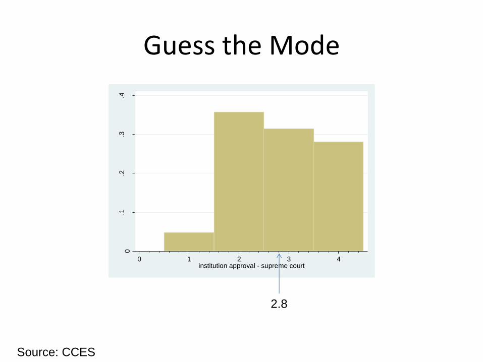
Guess the Mode
Source: CCES
0.1
.2.3
.4
Den
sity
0 1 2 3 4institution approval - supreme court
2.8

Guess the Mode
0
.2
.4
.6
.8
Fra
ctio
n
0 10 20 30Number of medals
3.3

Guess the Mode
Number of years the respondent has lived in his/her current home
0
.02
.04
.06
.08
Fra
ctio
n
0 20 40 60 80 100How long lived in current residence - Years

Guess the Mode
pew religion | Freq. Percent Cum.
--------------------------+-----------------------------------
protestant | 26,241 47.40 47.40
roman catholic | 12,348 22.30 69.70
mormon | 931 1.68 71.38
eastern or greek orthodox | 275 0.50 71.88
jewish | 1,678 3.03 74.91
muslim | 164 0.30 75.21
buddhist | 445 0.80 76.01
hindu | 89 0.16 76.17
agnostic | 2,885 5.21 81.38
nothing in particular | 7,641 13.80 95.18
something else | 2,667 4.82 100.00
--------------------------+-----------------------------------
Total | 55,364 100.00
The mode is rarely an informative statistic about the central tendency of the data.
It’s most useful in describing the “typical” observation of a categorical variable

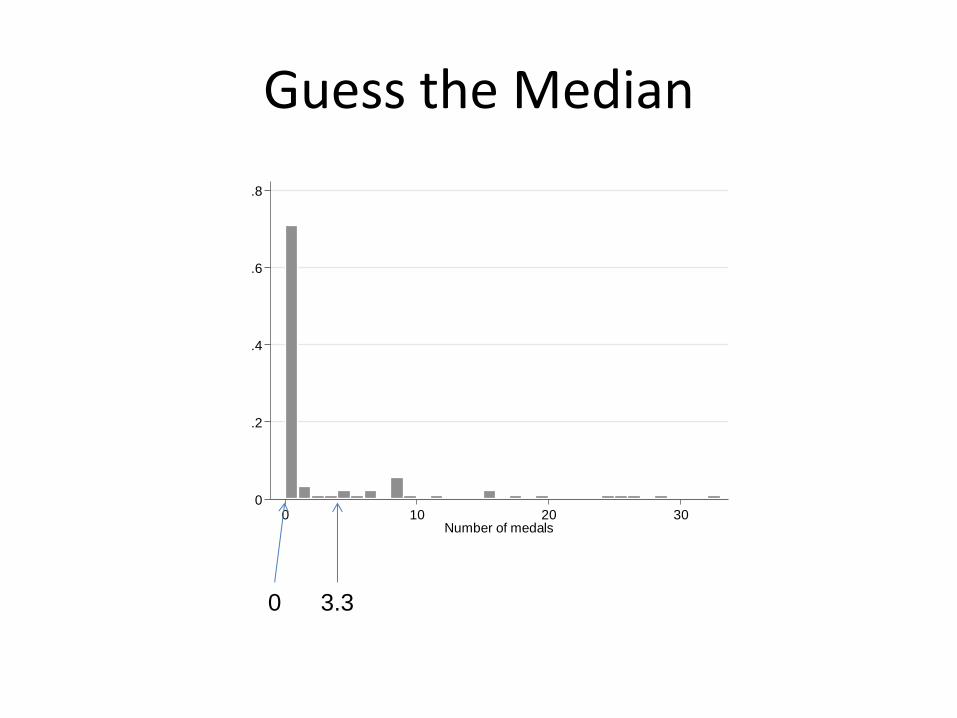
Median
• The numerical value separating the upper half of a distribution from the lower half of the distribution
– If N is odd, there is a unique median
– If N is even, there is no unique median --- the convention is to average the two middle values

Guess the Median
Source: CCES
0.1
.2.3
.4
Den
sity
0 1 2 3 4institution approval - supreme court
2.8 2.0

Guess the Median
Source: CCES
0.1
.2.3
.4
Den
sity
0 1 2 3 4institution approval - supreme court
2.8 2.0
3.0

Guess the Median
0
.2
.4
.6
.8
Fra
ctio
n
0 10 20 30Number of medals
3.3
Guess the Median
0
.2
.4
.6
.8
Fra
ctio
n
0 10 20 30Number of medals
3.3 0

Guess the Median
Number of years the respondent has lived in his/her current home
0
.02
.04
.06
.08
Fra
ctio
n
0 20 40 60 80 100How long lived in current residence - Years
Mode = 0
Mean = 11.8

Guess the Median
Number of years the respondent has lived in his/her current home
0
.02
.04
.06
.08
Fra
ctio
n
0 20 40 60 80 100How long lived in current residence - Years
Mode = 0
Mean = 11.8
Median = 8

Guess the Median
Number of years the respondent has lived in his/her current home
0
.02
.04
.06
.08
Fra
ctio
n
0 20 40 60 80 100How long lived in current residence - Years
Mode = 0
Mean = 11.8
Median = 8
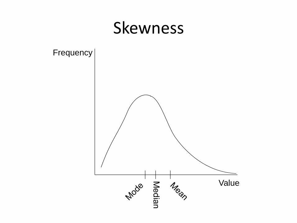
Note with right-skewed data:
Mode<median<mean

Median frequently preferred for income data

The (uninformative) graph
Mean = 68,735
Median = 35,000
Mode = 0 (probably)
0
1.0e-05
2.0e-05
3.0e-05
4.0e-05
5.0e-05
Den
sity
0 1.00e+07 2.00e+07 3.00e+07Income

Spread
• Range
– Max(x) – Min(x)
• Interquartile range (IQR)
– Q3(x) – Q1(x)
Q1 = CDF-1(.25)
Q3 = CDF-1(.75)
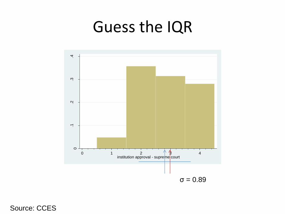
Guess the IQR
Source: CCES
0.1
.2.3
.4
Den
sity
0 1 2 3 4institution approval - supreme court
σ = 0.89

Guess the IQR
Source: CCES
0.1
.2.3
.4
Den
sity
0 1 2 3 4institution approval - supreme court
σ = 0.89
IQR = 2

Guess the IQR
Number of years the respondent has lived in his/her current home
0
.02
.04
.06
.08
Fra
ctio
n
0 20 40 60 80 100How long lived in current residence - Years
Mode = 0
Mean = 11.8
Median = 8
σ = 11.7

Guess the IQR
Number of years the respondent has lived in his/her current home
0
.02
.04
.06
.08
Fra
ctio
n
0 20 40 60 80 100How long lived in current residence - Years
Mode = 0
Mean = 11.8
Median = 8
σ = 11.7
IQR = 14 (17-3)

Don’t guess the IQR
0
.05
.1.1
5
Fra
ctio
n
0 10000000 20000000 30000000income
σ = 371,799
IQR = 50,000 (62,500-12,500)
Mean = 68,735
Median = 35,000
Mode = 0 (probably)

Lopsidedness and peakedness

Normal distribution example
• IQ
• SAT
• Height
• Symmetrical
• Mean = median = mode
Value
Frequency
22/)(
2
1)(
xexf

Skewness Asymmetrical distribution
• Income
• Contribution to candidates
• Populations of countries
• Age of MIT undergraduates
• “Positive skew”
• “Right skew” Value
Frequency

0.5
11
.5
Den
sity
0 5 10 15dividends_pc
Hyde County, SD
Distribution of the average $$ of dividends/tax return (in K’s)
0
.02
.04
.06
.08
.1
Den
sity
0 50 100 150var1
Fuel economy of cars for sale in
the US
Mitsubishi i-MiEV
(which is supposed to be all electric)
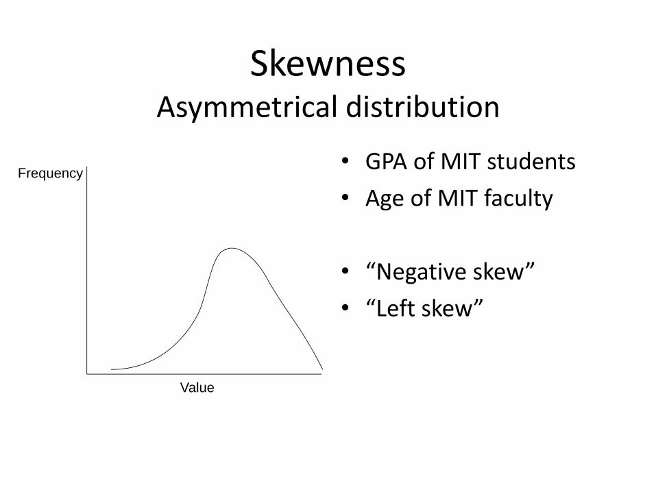
Skewness Asymmetrical distribution
• GPA of MIT students
• Age of MIT faculty
• “Negative skew”
• “Left skew”
Value
Frequency

Placement of Republican Party on 100-point scale
0
.02
.04
.06
.08
Den
sity
0 20 40 60 80 100place on ideological scale - republican party
Skewness
Value
Frequency

Guess the sign of the skew
Source: CCES
0.1
.2.3
.4
Den
sity
0 1 2 3 4institution approval - supreme court

Guess the sign of the skew
Source: CCES
0.1
.2.3
.4
Den
sity
0 1 2 3 4institution approval - supreme court
γ = 0.89
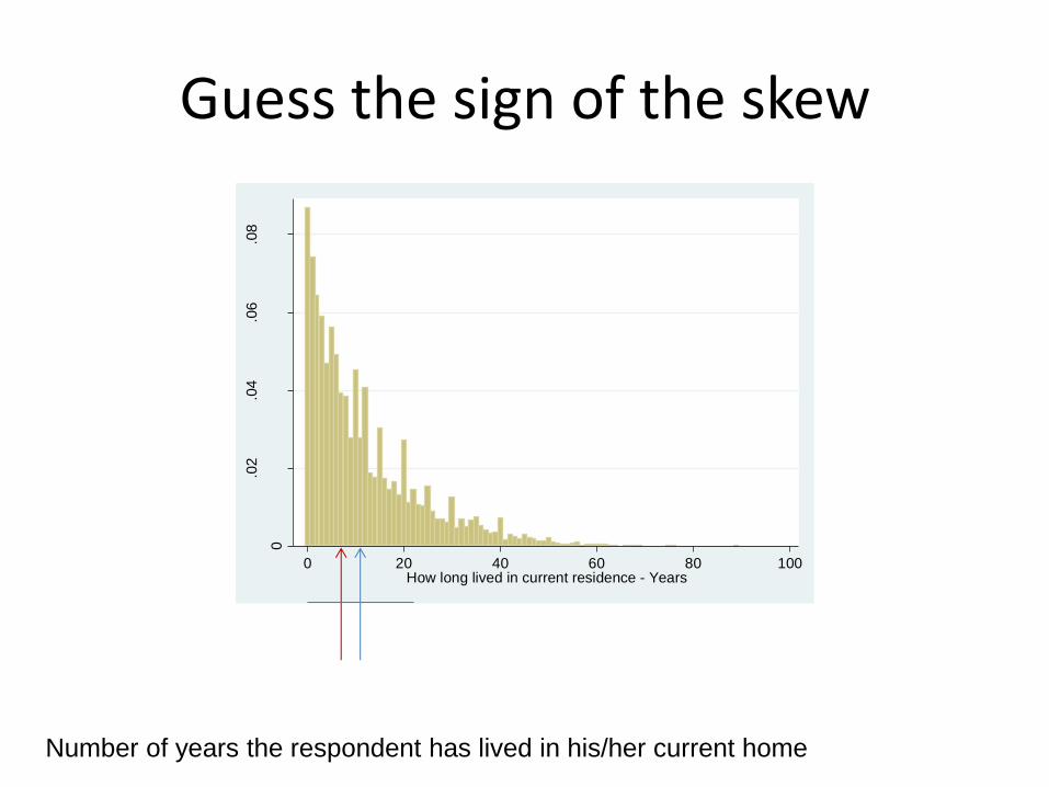
Guess the sign of the skew
Number of years the respondent has lived in his/her current home
0
.02
.04
.06
.08
Fra
ctio
n
0 20 40 60 80 100How long lived in current residence - Years

Guess the sign of the skew
Number of years the respondent has lived in his/her current home
0
.02
.04
.06
.08
Fra
ctio
n
0 20 40 60 80 100How long lived in current residence - Years
γ = 1.5

Note: It is really rare to find a naturally occurring variable with a
negative skew
0
.05
.1
.15
Fra
ctio
n
40 50 60 70 80Life expectancy
Mean = 68.3
s.d. = 8.7
Skew: -0.80

Kurtosis
Value
Frequency
k > 3
k = 3
k < 3
leptokurtic
platykurtic
mesokurtic

Mean s.d. Skew. Kurt.
Self-placement
4.5 1.9 -0.28 1.9
Dem. pty 2.2 1.4 1.1 3.9
Rep. pty 5.6 1.4 -0.98 3.7
Tea party 6.1 1.3 -2.1 7.5
Source: CCES, 2012
0
.05
.1.1
5.2
.25
Den
sity
0 2 4 6 8ideology - yourself
0.1
.2.3
.4
Den
sity
0 2 4 6 8ideology - dem party
0.1
.2.3
Den
sity
0 2 4 6 8ideology - rep party
0.2
.4.6
Den
sity
0 2 4 6 8ideology - tea party movement

Normal distribution
• Skewness = 0
• Kurtosis = 3
22/)(
2
1)(
xexf

Commands in STATA for univariate statistics (K&K pp. 176-186)
• summarize varlist
• summarize varlist, detail
• histogram varname, bin() start()
width() density/fraction/frequency
normal discrete
• table varname,contents(clist)
• tabstat
varlist,statistics(statname…)
• tabulate

. summ time_1
Variable | Obs Mean Std. Dev. Min Max
-------------+--------------------------------------------------------
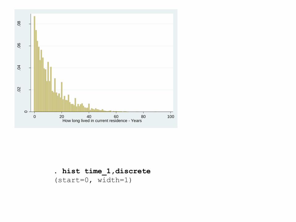
time_1 | 10153 11.78371 11.70837 0 89
. summ time_1,det
How long lived in current residence - Years
-------------------------------------------------------------
Percentiles Smallest
1% 0 0
5% 0 0
10% 1 0 Obs 10153
25% 3 0 Sum of Wgt. 10153
50% 8 Mean 11.78371
Largest Std. Dev. 11.70837
75% 17 69
90% 29 75 Variance 137.086
95% 36 76 Skewness 1.470977
99% 50 89 Kurtosis 5.21861
Data from 2012 Survey of the Performance of American Elections

. summ time_1
Variable | Obs Mean Std. Dev. Min Max
-------------+--------------------------------------------------------
time_1 | 10153 11.78371 11.70837 0 89
. summ time_1,det
How long lived in current residence - Years
-------------------------------------------------------------
Percentiles Smallest
1% 0 0
5% 0 0
10% 1 0 Obs 10153
25% 3 0 Sum of Wgt. 10153
50% 8 Mean 11.78371
Largest Std. Dev. 11.70837
75% 17 69
90% 29 75 Variance 137.086
95% 36 76 Skewness 1.470977
99% 50 89 Kurtosis 5.21861
Data from 2012 Survey of the Performance of American Elections
0
.02
.04
.06
.08
Den
sity
0 20 40 60 80 100How long lived in current residence - Years
. hist time_1,discrete
(start=0, width=1)
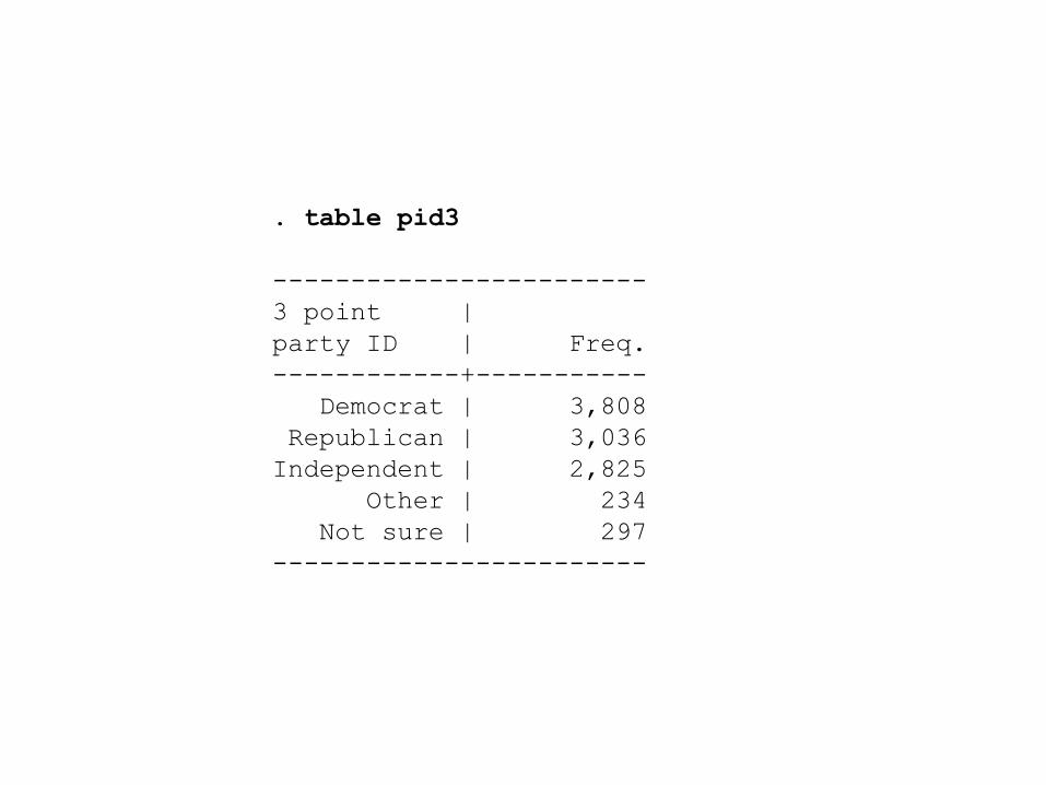
. table pid3
------------------------
3 point |
party ID | Freq.
------------+-----------
Democrat | 3,808
Republican | 3,036
Independent | 2,825
Other | 234
Not sure | 297
------------------------

. tabstat time_1 age
stats | time_1 age
---------+--------------------
mean | 11.78371 49.33363
------------------------------
. tabstat time_1 age,stats(mean sd skew kurt)
stats | time_1 age
---------+--------------------
mean | 11.78371 49.33363
sd | 11.70837 15.89716
skewness | 1.470977 -.0152461
kurtosis | 5.21861 2.177523
------------------------------

. tabstat time_1 age,by(pid3) s(mean sd)
Summary statistics: mean, sd
by categories of: pid3 (3 point party ID)
pid3 | time_1 age
------------+--------------------
Democrat | 11.28602 47.72348
| 11.7268 15.88458
------------+--------------------
Republican | 13.1379 52.27569
| 12.17941 15.69504
------------+--------------------
Independent | 11.66335 50.07646
| 11.35228 15.51778
------------+--------------------
Other | 8.457265 42.52991
| 9.328546 13.84282
------------+--------------------
Not sure | 8.084459 38.19865
| 9.559606 14.14754
------------+--------------------
Total | 11.78371 49.33363
| 11.70837 15.89716
---------------------------------

. table pid3,c(mean time_1 sd time_1)
----------------------------------------
3 point |
party ID | mean(time_1) sd(time_1)
------------+---------------------------
Democrat | 11.286 11.7268
Republican | 13.1379 12.17941
Independent | 11.6634 11.35228
Other | 8.45726 9.328546
Not sure | 8.08446 9.559606
----------------------------------------

Univariate graphs

Commands in STATA for univariate statistics
• histogram varname, bin()
start() width()
density/fraction/frequency
normal
• graph box varnames
• graph dot varnames
Example of Florida voters
• Question: does the age of voters vary by race?
• Combine Florida voter extract files, 2010
• gen new_birth_date=date(birth_date,"MDY")
• gen birth_year=year(new_b)
• gen age= 2010-birth_year

Look at distribution of birth year
0
.00
5.0
1.0
15
.02
.02
5
Den
sity
1850 1900 1950 2000birth_year

Explore age by race
. table race if birth_year>1900,c(mean age)
----------------------
race | mean(age)
----------+-----------
1 | 45.61229
2 | 42.89916
3 | 42.6952
4 | 45.09718
5 | 52.08628
6 | 44.77392
9 | 40.86704
---------------------- 3 = Black
4 = Hispanic
5 = White

Graph birth year
. hist age if birth_year>1900
(bin=71, start=9, width=1.3802817)
0
.01
.02
.03
Den
sity
0 20 40 60 80 100age

Graph birth year
. hist age if birth_year>1900
(bin=71, start=9, width=1.3802817)
0
.01
.02
.03
Den
sity
0 20 40 60 80 100age

Divide into “bins” so that each bar represents 1 year
. hist age if birth_year>1900,width(1)
0
.00
5.0
1.0
15
.02
Den
sity
0 20 40 60 80 100age

Add ticks at 10-year intervals
0
.00
5.0
1.0
15
.02
Den
sity
20 30 40 50 60 70 80 90 100age
. hist age if birth_year>1900,width(1) xlabel(20 (10) 100)
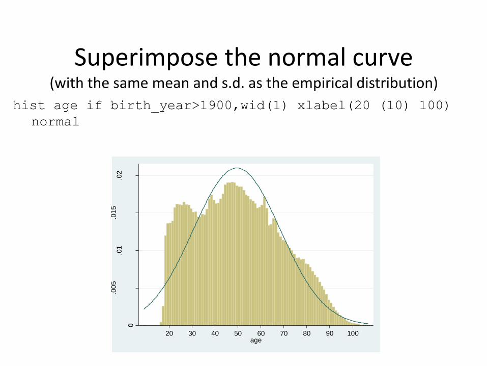
Superimpose the normal curve (with the same mean and s.d. as the empirical distribution)
hist age if birth_year>1900,wid(1) xlabel(20 (10) 100)
normal 0
.00
5.0
1.0
15
.02
Den
sity
20 30 40 50 60 70 80 90 100age

. summ age if birth_year>1900,det age ------------------------------------------------------------- Percentiles Smallest 1% 18 9 5% 21 16 10% 24 16 Obs 12612114 25% 34 16 Sum of Wgt. 12612114 50% 48 Mean 49.47549 Largest Std. Dev. 19.01049 75% 63 107 90% 77 107 Variance 361.3986 95% 83 107 Skewness .2629496 99% 91 107 Kurtosis 2.222442
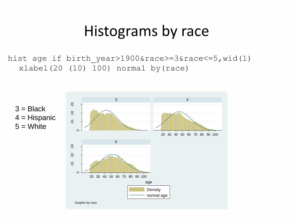
Histograms by race
hist age if birth_year>1900&race>=3&race<=5,wid(1)
xlabel(20 (10) 100) normal by(race) 0
.01
.02
.03
0
.01
.02
.03
20 30 40 50 60 70 80 90 100
20 30 40 50 60 70 80 90 100
3 4
5
Density
normal age
Den
sity
age
Graphs by race
3 = Black
4 = Hispanic
5 = White

05
01
00
age
Draw the previous graph with a box plot
graph box age if birth_year>1900
Upper quartile
Median
Lower quartile } Inter-quartile
range
} 1.5 x IQR
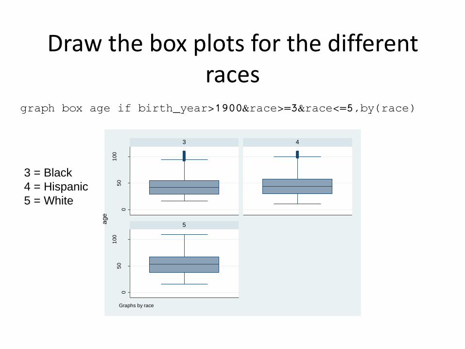
Draw the box plots for the different races
graph box age if birth_year>1900&race>=3&race<=5,by(race) 0
50
100
05
01
00
3 4
5age
Graphs by race
3 = Black
4 = Hispanic
5 = White

Draw the box plots for the different races using “over” option
graph box age if birth_year>1900&race>=3&race<=5,over(race) 0
50
100
age
3 4 5
3 = Black
4 = Hispanic
5 = White

Main issues with histograms
• Proper level of aggregation
• Non-regular data categories

Months Months Months
A
B
C
Stop and think:
What should the distribution of length-of-current residency
look like?
(Hint: the median is around 4 years)

A note about histograms with unnatural categories
From the Current Population Survey (2000), Voter and Registration Survey How long (have you/has name) lived at this address? -9 No Response -3 Refused -2 Don't know -1 Not in universe 1 Less than 1 month 2 1-6 months 3 7-11 months 4 1-2 years 5 3-4 years 6 5 years or longer

Solution, Step 1 Map artificial category onto “natural”
midpoint
-9 No Response missing
-3 Refused missing
-2 Don't know missing
-1 Not in universe missing
1 Less than 1 month 1/24 = 0.042
2 1-6 months 3.5/12 = 0.29
3 7-11 months 9/12 = 0.75
4 1-2 years 1.5
5 3-4 years 3.5
6 5 years or longer 10 (arbitrary)
recode live_length (min/-1 =.)(1=.042)(2=.29)(3=.75)(4=1.5) ///
(5=3.5)(6=10)

Graph of recoded data F
ract
ion
longevity0 1 2 3 4 5 6 7 8 9 10
0
.557134
histogram longevity, fraction

Graph of recoded data
Fra
ctio
n
longevity0 1 2 3 4 5 6 7 8 9 10
0
.557134
Why doesn’t…
…look like …
?

longevity
0 1 2 3 4 5 6 7 8 9 10
0
15
Density plot of data
Total area of last bar = .557
Width of bar = 11 (arbitrary)
Solve for: a = w h (or)
.557 = 11h => h = .051

Density plot template
Category Fraction X-min X-max X-length
Height
(density)
< 1 mo. .0156 0 1/12 .082 .19*
1-6 mo. .0909 1/12 ½ .417 .22
7-11 mo. .0430 ½ 1 .500 .09
1-2 yr. .1529 1 2 1 .15
3-4 yr. .1404 2 4 2 .07
5+ yr. .5571 4 15 11 .05
* = .0156/.082

Three words about pie charts: don’t use them

So, what’s wrong with them
• For non-time series data, hard to get a comparison among groups; the eye is very bad in judging relative size of circle slices
• For time series, data, hard to grasp cross-time comparisons

Some words about graphical presentation
• Aspects of graphical integrity (following Edward Tufte, Visual Display of Quantitative Information)
– Main point should be readily apparent
– Show as much data as possible
– Write clear labels on the graph
– Show data variation, not design variation
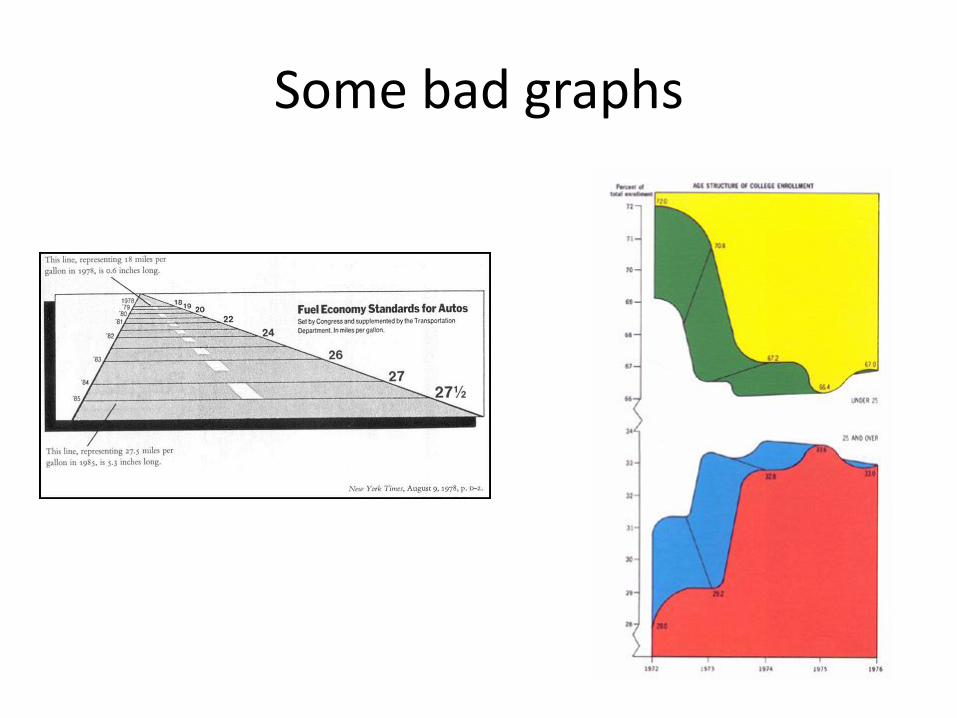
Some bad graphs

Some good graphs

Download and use the “Tufte” scheme
• ssc install scheme_tufte
.2.3
.4.5
.6.7
de
mp
resp
ct2
00
0
.3 .4 .5 .6 .7demprespct1964
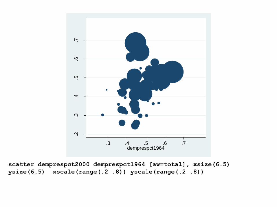
scatter demprespct2000 demprespct1964 [aw=total], xsize(6.5)
ysize(6.5) xscale(range(.2 .8)) yscale(range(.2 .8))

.2
.3
.4
.5
.6
.7
de
mp
resp
ct2
00
0
.3 .4 .5 .6 .7demprespct1964
scatter demprespct2000 demprespct1964 [aw=total], xsize(6.5)
ysize(6.5) xscale(range(.2 .8)) yscale(range(.2 .8)) scheme(tufte)

There is a difference between graphs in research and publication
0
.01
.02
.03
0
.01
.02
.03
20 30 40 50 60 70 80 90 100
20 30 40 50 60 70 80 90 100
3 4
5
Density
normal age
Den
sity
age
Graphs by race
0
.01
.02
.03
0
.01
.02
.03
20 30 40 50 60 70 80 90 100 20 30 40 50 60 70 80 90 100
Black Hispanic
White Total
Den
sity
AgeGraphs by race
Do not publish
Publish OK