Introduction Fracture Mechanics Fatigue Crack · PDF fileI Assessment Handbook , FAA Technical...

DOT/FAA/CT-93/69. I Damage Tolerance

Atlantic City Airport, Volume I: Introduction Assessment Handbook DOT-VNTSC-FAA-93-13. I

, FAA Technical Center

NJ 08405 Fracture Mechanics Fatigue Crack Propagation

Research and Special Programs Administration John A. Volpe National Transportation Systems Center Cambridge, MA 02142-1 093

8

Final Report October 1993

I This document is available to the public through the National Technical Information Service Springfield, Virginia 22161 .'

U.S. Department of Transportation Federal Avlation Adrnlnlstratlon

94 1 19 025

REPORT DOCUMENTATION PAGE 1

FormAp roved OMB No. d204-0188

P@lic report ing bur- fo r t h i s co l lect ion of in fomet ion i s e s t i m t e d t o average 1 hour per r e a s , ineldim the ti= for r w i e u i n g instruct ions searchi ex is t f data soUrces, gathering a@ m i n t a i n i n g the t a needed, nd c w l e t i m ard revieuina the coflect ion 2 i n f o d i m . Send conrnents r w a r d i m t h i s burden estimate or YIY other

1. AGENCY USE OtiLY (Leave .blank) 2. REPORT DATE I October 1993 3. REPORT TYPE AND DATES COVERED I June 1990 - Dec. 1992

4 . TITLE AND SUETITLE Damage Tolerance Assessment Handbook ~~

I 5. FLINDING NWBERS

Fh3H2/A3128 Volume I: Introduction Fracture Mechanics Fatigue Crack Propagation

6. AUTHOR(S)

7. PERFORMING O U G M l U T I O L I NAME(S) AND ADDRESS(ES1 U.S. Department o f Transportation Research and Special Progrems Adninistration Volpe National Transportation S y s t e m s Center Kcndell Square, C d r i d g e , MA 02162

8. PERFORMING ORCWIUTlW REPOUT NWBER

DOT-VNTSC-FAA-93-13.1

9. SPOUSORING/IK)WITORING AGENCY NAME(S) AND ADDRESSCES) Federal Aviation Administration Technical Center

Atlantic City Airport NJ 08405

10. SPOUSORIYG/IIIWIITORING AGENCY REPORT NUMBER

DOT/FAA/CT-93/69.1

11. SUPPLEMENTARY NOTES

121. DlSTRlBUTIOY/AVAILABILITY STATEMENT 12b. DISTRIBUTIOY COO€

This document is available to the public through the National Technical Infoqnation Service, Springfield, VA 22161

13. ABSTRACT (Haxinun 200 words)

This "Damage Tolerance Assessment Handbook" consists of two volumes:

Volume I introduces the damage tolerance concept with a historical perspective followed by the fundamentals of fracture mechanics and fatigue crack propagation. Various fracture criteria and crack growth rules are studied.

Volume I1 treats exclusively the subject of damage tolerance evaluation of airframes

14. SUBJECT TERMS Dmmge Tolerance, Fracture Mechanics, Crack In i t i a t i on , Fracture Toughness, Stress In tens i ty Factor, Residual Strength, Crack Propagation, Fatigue, Inspection.

15. NWBER OF PAGES

I 16. PRICE CODE 1

I 1

17. SECURITY CLASSIFICATIW 18. SECURITY CLASSIFICATIOLI 19. SECURITY CLASSIFIUTIOW 20. LlWlTATlOY OF ABSTRACT OF REPORT OF THIS PAGE OF ABSTRACT Unclassified Unclassified Unclas s if ied

Sta r Form (Rev. - P r e s 5 i L bv Std. t 3 P h 298-102

PREFACE

The preparation of this Handbook has required the cooperation of numerous individuals from the U.S. Government, universities, and industry. It is the outcome of one of the research programs on the Structural Integrity of Aging Aircraft supported by the Federal Aviation Administration Technical Center and performed at the Volpe Center of the Department of Transportation.

The contributions fiom the Federal Aviation Administration, the FAA Technical Center, the Department of Defense, and the staff of the Volpe Center are greatly acknowledged.

Please forward all comments and suggestions to : I Accesion For I

NTIS CRA&I DTlC TAB

Volpe National Transportation Systems Center

U.S. Department of Transportation Office of Systems Engineering, DTS-74

Cambridge, MA 02 142

... 111

Avail and lo r

~ ~ ~~~ ~~

METRIUENGLISH CONVERSION FACTORS

ENGLISH T O METRIC

LENGTH (APPROXIMATE) 1 inch (in.) = 2.5 centimeters (cm) 1 foot (ft) = 30 Centimeters (cm)

1 yard (yd) = 0 9 meter (m) 1 mile (mi) = 1.6 kilometers (km)

A R E A (APPROXIMATE) 1 square inch (sq in, in21 = 6.5 square centimeters (cm2) 1 square foot (sq ft, ft2) = 0 09 square meter (m2)

1 square yard (sq yd. yd2) = 0.8 square meter (m2) 1 square mile (sq mi, mi21 = 2.6 square kilometers (km2) 1 acre = 0 4 hectares (he) = 4,000 square meters (m2)

M A S S - W E I G H T (APPROXIMATE) 1 ounce (02) = 28 grams (gr) 1 pound (Ib) = 45 kilogram (kg)

1 short ton = 2,000 pounds (Ib) = 0 9 tonne (t)

VOLUME*(APPROXIMATE) 1 teaspoon (tsp) = 5 milliliters (ml)

1 tablespoon (tbsp) = 15 milliliters (rnl) 1 fluid ounce (fl OZ) = 30 milliliters (ml)

1 cup (c) = 0 24 liter (I) i p i n t (pt) = o 47 liter (I)

1 quart (qt) = 0 96 liter (I) 1 gallon (gal) = 3 8 liters (I)

1 cubic foot (cu ft, ft3) = 0 03 cubic meter (m3) 1 cubic yard (cu yd, yd3) = 0 76 cubic meter (m3)

TEMPERATURE (EXACT) [ (x - 32) (5i9) I O F = y"C

METRIC T O ENGLISH

LENGTH (APPROXIMATE) 1 millimeter (mm) = 0.04 inch (in) 1 centimeter (cm) = 0.4 inch (in)

1 meter (m) = 3.3 feet (ft) 1 meter (m) = 1 .l yards (yd)

1 kilometer (km) = 0.6 mile (mi)

A R E A (APPROXIMATE) 1 square centimeter (cm2) = 0.16 square inch (sq in, in2)

1 square meter (m2) = 1.2 square yards (sq yd, yd2) 1 square kilometer (knz) = 0.4square mile (sq mi, mi2) 1 hectare (he) = 10,000 square meters (m2) = 2.5 acres

M A S S - W E I G H T (APPROXIMATE) 1 gram (gr) = 0.036 ounce (oz)

1 kilogram (kg) = 2.2 pounds (Ib) 1 tonne(t) = 1,000 kilograms(kg) = 1.1 shorttons

V O L U M E (APPROXIMATE) 1 milliliter (ml) = 0.03 fluid ounce (fl oz)

1 liter(1) = 2.1 pints(pt) 1 liter (I) = 1.06 quarts (qt) 1 liter (I) = 0.26 gallon (gal)

1 cubic meter (m3) = 36 cubic feet (tuft, f t 3 ) 1 cubic meter (m3) = 1.3 cubic yards (cu yd, yd3)

TEMPERATURE (EXACT) [(9/5)y + 32 1°C = x O F

QUICK INCH-CENTIMETER LENGTH CONVERSION

1 2 3 4 5 6 7 8 9 10 INCHES I I I I I I I

ENTIMETERS 0 1 2 3 4 5 6 7 8 9 10 11 12 13 14 15 I6 17 18 19 20 2 1 22 23 24

25.40

QU ICK F A H RE N H E IT-CE LSI US TEMPERATURE CONVERSION

-roo -no 4 0 14' 32' 50' 68' 86O 104' 122' 140' 158* 176' 194' 212' OF I I I I I I I I I I I I I I I

I I I I I O C 40' -30' -10' .IOo 0' 10' 20' IO0 40' 50' 60' 70' 80' 90' looo

For more e x a c and or other convers ion faCtors, see NBS Miscellaneous Publication 286, Units of Weights and Measures Price 52.50 SDCatalog No C13 10286.

iv

TABLE OF CONTENTS

i

1 . INTRODUCTION . . . . . . . . . . . . . . . . . . . . . . . . . . . . . . . . . . . . . . . . . . . . 1 . 1

1.1 Historical Perspective . . . . . . . . . . . . . . . . . . . . . . . . . . . . . . . . . . . . . . 1-2 1.2 Results of Air Force Survey . . . . . . . . . . . . . . . . . . . . . . . . . . . . . . . . 1-12 1.3 Comparison of Old and New Approaches . . . . . . . . . . . . . . . . . . . . . . . 1-13

1.3.1 Fatigue Safe-Life Approach . . . . . . . . . . . . . . . . . . . . . . . . . . . 1-16 1.3.2 Damage Tolerance Assessment (DTA) Approach . . . . . . . . . . . . . 1-25

2 . FRACTURE MECHANICS . . . . . . . . . . . . . . . . . . . . . . . . . . . . . . . . . . . . . 2-1

2.1 Stress Concentration. Fracture and Griffith Theory . . . . . . . . . . . . . . . . . . 2-1

2.1.1 Fracture Modes . . . . . . . . . . . . . . . . . . . . . . . . . . . . . . . . . . . . 2-19

2.2 Extension of Linear Elastic Fracture Mechanics to Metals . . . . . . . . . . . . 2-21

2.2.1 Plastic Zone Size and the Mises-Hencky Yield Criterion . . . . . . . 2-24

2.3 Fracture Toughness Testing . . . . . . . . . . . . . . . . . . . . . . . . . . . . . . . . . . 2-26

2.3.1 Thickness Effects . . . . . . . . . . . . . . . . . . . . . . . . . . . . . . . . . . 2-33 2.3.2 Temperature Effects . . . . . . . . . . . . . . . . . . . . . . . . . . . . . . . . . 2-37

2.4 Failure in the Presence of Large-Scale Yielding . . . . . . . . . . . . . . . . . . . 2-38

2.4.1 Resistance Curves . . . . . . . . . . . . . . . . . . . . . . . . . . . . . . . . . . 2-39

2.4.1.1 Graphical Construction of Thin-Section Strength Plots . 2-43

2.4.2 The Net Section Failure Criterion . . . . . . . . . . . . . . . . . . . . . . . 2-52

2.4.2.1 Failure Mode Determination and the Feddersen Diagram 2-54

2.4.3 Crack Opening Displacement . . . . . . . . . . . . . . . . . . . . . . . . . . 2-56 2.4.4 J-Integral . . . . . . . . . . . . . . . . . . . . . . . . . . . . . . . . . . . . . . . . . 2-57 2.4.5 Practical Developments . . . . . . . . . . . . . . . . . . . . . . . . . . . . . . . 2-58 2.4.6 Strain Energy Density Criterion . . . . . . . . . . . . . . . . . . . . . . . . . 2-61 2.4.7 Plastic Collapse Model . . . . . . . . . . . . . . . . . . . . . . . . . . . . . . . . 2-64

2.5 Internal. Surface. and Comer Cracks . . . . . . . . . . . . . . . . . . . . . . . . . . 2-66 2.6 Environmental Effects . . . . . . . . . . . . . . . . . . . . . . . . . . . . . . . . . . . . 2-67

V

TABLE OF CONTENTS (continued)

3 . FATIGUE CRACK PROPAGATION . . . . . . . . . . . . . . . . . . . . . . . . . . . . . . 3-1

3.1 Energy-Based Theory of Crack Propagation . . . . . . . . . . . . . . . . . . . . . . 3-1 3.2 Empirical Crack Growth Rate Equations . . . . . . . . . . . . . . . . . . . . . . . . . 3-3 3.3 Correlation with Material Properties . . . . . . . . . . . . . . . . . . . . . . . . . . . 3-12 3.4 Crack Growth Life Estimates . . . . . . . . . . . . . . . . . . . . . . . . . . . . . . . 3-32

3.4.1 Quick Estimates with Crack Geometry Sums . . . . . . . . . . . . . . . 3-37

3.5 Interaction Effects and Retardation Models . . . . . . . . . . . . . . . . . . . . . . 3-38

4 . AIRFRAME DAMAGE TOLERANCE EVALUATION . . . . . . . . . . . . . . . . . 4-1

4.1 Damage Tolerance Requirements for Transports . . . . . . . . . . . . . . . . . . . 4-2

4.1.1 Basic Definitions . . . . . . . . . . . . . . . . . . . . . . . . . . . . . . . . . . . . 4-2 4.1.2 The Damage Tolerance Evaluation Process . . . . . . . . . . . . . . . . . . 4-2

4.1:2.1 Preparation Phase . . . . . . . . . . . . . . . . . . . . . . . . . . . . 4-5 4.1.2.2 Evaluation Phase . . . . . . . . . . . . . . . . . . . . . . . . . . . . 4-7 4.1.2.3 Inspectability Considerations . . . . . . . . . . . . . . . . . . . . 4-9

b

4.2 Identification of Structural Elements and Evaluation Locations . . . . . . . . 4-10

4.2.1 Wing and Empennage . . . . . . . . . . . . . . . . . . . . . . . . . . . . . . . 4-12 4.2.2 Fuselage . . . . . . . . . . . . . . . . . . . . . . . . . . . . . . . . . . . . . . . . . 4-18

4.3 Load Path Arrangement . . . . . . . . . . . . . . . . . . . . . . . . . . . . . . . . . . . 4-33

4.3.1 Splices Parallel to the Major Stress Axis . . . . . . . . . . . . . . . . . . 4-34 4.3.2 Stiffeners as Crack Stoppers . . . . . . . . . . . . . . . . . . . . . . . . . . . 4-41 4.3.3 Splices Across the Major Load Axis . . . . . . . . . . . . . . . . . . . . . . 4-51

4.3.3.1 Load Concentration and the Benefit of Fastener Flexibility . . . . . . . . . . . . . . . . . . . . . . . . . . . . . . . . 4-54

4.3.4 Repairs . . . . . . . . . . . . . . . . . . . . . . . . . . . . . . . . . . . . . . . . . . 4-65

4.4 Material Considerations . . . . . . . . . . . . . . . . . . . . . . . . . . . . . . . . . . . 4-69

4.6 Analysis and Tests . . . . . . . . . . . . . . . . . . . . . . . . . . . . . . . . . . . . . . . 4-86 4.5 Type and Extent of Damage . . . . . . . . . . . . . . . . . . . . . . . . . . . . . . . . 4-73

vi

TABLE OF CONTENTS (continued)

4.6.1 Load Specification and Stress Analysis . . . . . . . . . . . . . . . . . . . 4-86

4.6.1.1 Gust Load Factors (FAR 23.231 and FAR 25.341) . . . . 4-92

4.6.2 Residual Strength Evaluation . . . . . . . . . . . . . . . . . . . . . . . . . . 4-98 4.6.3 Crack Growth Life Evaluation . . . . . . . . . . . . . . . . . . . . . . . . . . 4-122

4.6.3.1 Modified Safe Life Based on Crack Growth . . . . . . . . . 4-122 4.6.3.2 Damage Tolerance Evaluation Requiring Inspection . . . 4-125

4.6.3.2.1 General Considerations for Nondestructive Inspection (NDI) Methodologies and the Inspection Intervals [Reference 4-13] . . . . 4-125 Time to First Inspection and Safe Inspection Interval . . . . . . . . . . . . . . . . . . . . . . . . . . 4- 126

4.6.3.2.2

4.6.3.3 Safe Flight Time After Discrete Source Damage . . . . . 4-129 4.6?3.4 Time to Loss of Fail-Safety .................... 4-131 4.6.3.5 Verification of Crack Growth Life . . . . . . . . . . . . . . . 4-135

4.6.3.5.1 Approximate Estimation of Spectrum Truncation Points . . . . . . . . . . . . . . . . . . . 4- 141

APPENDIX A . SELECTED STRESS INTENSITY FACTOR FORMULAE . . . . . . A-1

APPENDIX B . SELECTED RESISTANCE (R-CURVE) PLOTS FOR AIRCRAFT MATERIALS . . . . . . . . . . . . . . . . . . . . . . . . . . . . . . . . . . . . . . . . B-1

vii

LIST OF ILLUSTRATIONS

1-1 1-2 1-3 1-4

1-5

1-6 1-7

1-8 1-9 1-10 1-1 1 1-12 1-13 1-14 1-15 1-16 1-17 1-18 2- 1 2-2 2- 3

2-4

2-5 2-6 2-7

2-8 2-9

Photograph of tanker Schenectady . . . . . . . . . . . . . . . . . . . . . . . . . . . . . . . . 1-3 Comet I aircraft. circa 1952 . . . . . . . . . . . . . . . . . . . . . . . . . . . . . . . . . . . . 1-3 Probable Comet failure initiation site . . . . . . . . . . . . . . . . . . . . . . . . . . . . . . 1-4 USAF Tactical Air Command F-11 1A circa 1969 .

(a) F-111 in flight . . . . . . . . . . . . . . . . . . . . . . . . . . . . . . . . . . . . . . 1-8 (b) F.111. plan view showing probable failure initiation site . . . . . . . . . 1-8 (c) Crack in left wing pivot forging of F-111 aircraft . . . . . . . . . . . . . 1-8

(a) General view. left side of forward fuselage . . . . . . . . . . . . . . . . . . 1-10 (b) General view. right side of forward fuselage . . . . . . . . . . . . . . . . . 1-10

1-14

(a) 1226 major crackinglfailure incidents . . . . . . . . . . . . . . . . . . . . . 1 . 14 (b) 64 major crackinglfailure incidents . . . . . . . . . . . . . . . . . . . . . . . 1 . 14

Cracking and failure origins . . . . . . . . . . . . . . . . . . . . . . . . . . . . . . . . . . . 1-15 Results of a typical fatigue experiment . . . . . . . . . . . . . . . . . . . . . . . . . . . 1 . 16 Effect of mean stress . . . . . . . . . . . . . . . . . . . . . . . . . . . . . . . . . . . . . . . . 1-18 Modified Goodman diagram . . . . . . . . . . . . . . . . . . . . . . . . . . . . . . . . . . . 1-19 Goodman diagram for 2024-T4 aluminum . . . . . . . . . . . . . . . . . . . . . . . . . 1-19 How the Palmgren-Miner rule is applied . . . . . . . . . . . . . . . . . . . . . . . . . . 1-21 Fatigue quality index . . . . . . . . . . . . . . . . . . . . . . . . . . . . . . . . . . . . . . . . 1-23 Uncertainties addressed by safety factor . . . . . . . . . . . . . . . . . . . . . . . . . . . 1-24 Crack growth in response to cyclic loads . . . . . . . . . . . . . . . . . . . . . . . . . . 1-26 Schematic relationship of allowable stress versus crack length . . . . . . . . . . . 1-26 Residual strength diagram . . . . . . . . . . . . . . . . . . . . . . . . . . . . . . . . . . . . 1-27 Circular hole in a large plate . . . . . . . . . . . . . . . . . . . . . . . . . . . . . . . . . . . 2-2 Elliptical hole in a large plate . . . . . . . . . . . . . . . . . . . . . . . . . . . . . . . . . . . 2-3 Ene.rgy principles .

(a) Slender rod . . . . . . . . . . . . . . . . . . . . . . . . . . . . . . . . . . . . . . . . 2-6 (b) Uniformly stressed thin plate . . . . . . . . . . . . . . . . . . . . . . . . . . . . 2-6

(a) Initial crack length 2a . . . . . . . . . . . . . . . . . . . . . . . . . . . . . . . . . . 2-9 (b) Elongated crack length 2(a + Aa) . . . . . . . . . . . . . . . . . . . . . . . . . 2-9

Plate with a center crack . . . . . . . . . . . . . . . . . . . . . . . . . . . . . . . . . . . . . 2-11 Stress components in Irwin’s analysis . . . . . . . . . . . . . . . . . . . . . . . . . . . . 2-14 Stress intensity factor formulae for some common geometiies .

An aircraft fuselage failure

Examples of distribution and magnitude of service cracking problems . . . . . . Crack initiatiodgrowth and failure mechanisms .

Energy principles for cracked plate .

(a) Plate with center crack under tension . . . . . . . . . . . . . . . . . . . . . 2-17 (b) Plate with edge crack under tension . . . . . . . . . . . . . . . . . . . . . . 2-17

Fracture modes . . . . . . . . . . . . . . . . . . . . . . . . . . . . . . . . . . . . . . . . . . . . 2-20 2-23 Plastic zone formation ahead of crack tip . . . . . . . . . . . . . . . . . . . . . . . . . .

... V l l l

LIST OF ILLUSTRATIONS (continued)

2-10 2-1 1 2-12 2-13 2-14 2-15 2-16 2-17

2-18 2-19 2-20 2-2 1 2-22 2-23 2-24 2-25 2-26 2-27 2-28 2-29 2-30 2-3 1 2-32 2-33

2-34 2-35 2-36 2-37 2-38

2-39 2-40 2-41

Refined estimate of plastic zone formation ahead of crack tip . . . . . . . . . . . . Plastic zone approximations based on von Mises criterion The compact tension specimen . . . . . . . . . . . . . . . . . . . . . . . . . . . . . . . . . CTS stress intensity factor versus crack length CTS orientation . . . . . . . . . . . . . . . . . . . . . . . . . . . . . . . . . . . . . . . . . . . Load-displacement plot . . . . . . . . . . . . . . . . . . . . . . . . . . . . . . . . . . . . . . Thickness effect on fracture strength

. . . . . . . . . . . . . .

. . . . . . . . . . . . . . . . . . . . . .

. . . . . . . . . . . . . . . . . . . . . . . . . . . . . Plane stress-plane strain transition .

(a) Three-dimensional plastic zone shape . . . . . . . . . . . . . . . . . . . . . (b) Plastic volume versus thickness . . . . . . . . . . . . . . . . . . . . . . . . .

Typical fracture surfaces . . . . . . . . . . . . . . . . . . . . . . . . . . . . . . . . . . . . . Lateral compression above and below the crack . . . . . . . . . . . . . . . . . . . . .

Fracture toughness versus temperature . . . . . . . : . . . . . . . . . . . . . . . . . . . . Load versus crack extension for different thicknesses . . . . . . . . . . . . . . . . . Experimental determination of R-curve . . . . . . . . . . . . . . . . . . . . . . . . . . . Dependence of K , on crack length . . . . . . . . . . . . . . . . . . . . . . . . . . . . . . .

KI and KR curves (logarithmic scale) . . . . . . . . . . . . . . . . . . . . . . . . . . . . . . Overlay of KI and KR curves to determine critical crack length . . . . . . . . . . . R-Curve for 2024-T3 . . . . . . . . . . . . . . . . . . . . . . . . . . . . . . . . . . . . . . . . K applied versus crack length . . . . . . . . . . . . . . . . . . . . . . . . . . . . . . . . . . Use of critical K to determine critical crack length . . . . . . . . . . . . . . . . . . . Critical stress determinations with KI and KR curves . . . . . . . . . . . . . . . . . . K, and 0. vs . a for a 20-inch aluminum panel . . . . . . . . . . . . . . . . . . . . . . Effect of surroundings on energy absorption rate .

(a) Isolated medium or long crack . . . . . . . . . . . . . . . . . . . . . . . . . .

(c) One crack tip near edge of a panel . . . . . . . . . . . . . . . . . . . . . . . Net section failure criterion . . . . . . . . . . . . . . . . . . . . . . . . . . . . . . . . . . . Net section and R-curve strength curves . . . . . . . . . . . . . . . . . . . . . . . . . . Illustration of the width effect on thin sheet strength . . . . . . . . . . . . . . . . . . Construction of Feddersen diagram . . . . . . . . . . . . . . . . . . . . . . . . . . . . . . Typical examples of three-dimensional aspects of cracks .

(a) Comer crack at a fastener hole . . . . . . . . . . . . . . . . . . . . . . . . . . (b) Axial crack in an oxygen cylinder . . . . . . . . : . . . . . . . . . . . . . . . (c) Through-crack at a fuselage frame comer detail . . . . . . . . . . . . . .

Strain energy density criterion . . . . . . . . . . . . . . . . . . . . . . . . . . . . . . . . . Definition of critical strain energy density . . . . . . . . . . . . . . . . . . . . . . . . . Erdogan’s plastic zone model . . . . . . . . . . . . . . . . . . . . . . . . . . . . . . . . . .

Lateral buckling and tearing . . . . . . . . . . . . . . . . . . . . . . . . . . . . . . . . . . .

KI and KR curves . . . . . . . . . . . . . . . . . . . . . . . . . . . . . . . . . . . . . . . . . . .

. . . . . . . . . . . . . . . . . . . . . . . . . . . . . . . . . . . . . . . . (b) Shortcrack

2-23 2-25 2-27 2-28 2-29

2-33 2-30

2-35 2-35 2-36 2-37 2-38 2y39 2-40 2-42 2-43 2-44 2-44 2-45 2-46 2-47 2-48 2-49 2-50

2-51 2-51 2-51 2-53 2-54 2-55 2-56

2-60 2-60 2-60 2-63 2-63 2-65

ix


2-42

2-43 2-44 3-1

3-2

3-3 3-4 3-5 3-6 3-7 3-8 3-9

3-10 3-1 1

3-12 3-13 3-14

4- 1 4-2 4-3 4-4 4-5 4- 6 4-7 4-8 4-9 4-10

Geometries of surface and comer cracks . (a) Flaw shape parameter for surface flaws .................... (b) Flaw shape parameter for internal flaws ....................

Stress intensity factors for surface and comer cracks . . . . . . . . . . . . . . . . . . Deep flaw magnification factor curves . . . . . . . . . . . . . . . . . . . . . . . . . . . . Argument for relating fatigue crack growth rate to applied stress intensity factor . . . . . . . . . . . . . . . . . . . . . . . . . . . . . . . . . . . . . . . . . . . . . . . . . . . . Effect of cyclic load range on crack growth in Ni-Mo-V alloy steel for released tension loading . . . . . . . . . . . . . . . . . . . . . . . . . . . . . . . . . . . . . . . Alternate definitions of stress cycle . . . . . . . . . . . . . . . . . . . . . . . . . . . . . . . Crack growth rate in 7475-T6 aluminum . . . . . . . . . . . . . . . . . . . . . . . . . . . Effect of stress ratio on 7075-T6 aluminum crack growth rate . . . . . . . . . . . . Summary plot of dddN versus AK for six aluminum alloys . . . . . . . . . . . . . Summary plot of dddN versus AK for various steel alloys . . . . . . . . . . . . . . Summary plot of dddN versus AK for five titanium alloys . . . . . . . . . . . . . 7075-T6 aluminum (0.09 in . thick) crack growth rate properties .

(a) Results for R = 0 and R = 0.2 (b) Results for R = 0.33 and R = 0.5 . . . . . . . . . . . . . . . . . . . . . . . . (c) Results for R = 0.7 and R = 0.8

. . . . . . . . . . . . . . . . . . . . . . . . . .

. . . . . . . . . . . . . . . . . . . . . . . . . 7075-T6 properties (0.2 in . thick) from a different test series . . . . . . . . . . . . 2024T3 aluminum (0.09 in . thick) properties .

(a) Results for R = 0.1 and R = 0.11 (different test series) (b) Results for R = 0.33 . . . . . . . . . . . . . . . . . . . . . . . . . . . . . . . . . (c) Results for R = 0.5 . . . . . . . . . . . . . . . . . . . . . . . . . . . . . . . . . . (d) Results for R = 0.7 . . . . . . . . . . . . . . . . . . . . . . . . . . . . . . . . . .

2014-T6 aluminum (0.25 in . thick) properties at R = 0 2014-T6 aluminum properties for different thickness and stress ratio . . . . . . .

(a) Effect of thickness on FCP behaviour of 7475T651 machined from 1-inch plate and tested in dry air .....................

(b) A comparison between the FCP rates in dry air and 3.5% NaCl solution for aluminum alloys ............................

Structure of requirements and guidelines Structural classification of an airframe . . . . . . . . . . . . . . . . . . . . . . . . . . . . Wing box configuration and function . . . . . . . . . . . . . . . . . . . . . . . . . . . . . Stress in a wing box Simplified fuselage model . . . . . . . . . . . . . . . . . . . . . . . . . . . . . . . . . . . . Stress in a fuselage shell Framebending . . . . . . . . . . . . . . . . . . . . . . . . . . . . . . . . . . . . . . . . . . . . Floor cross-beam function . . . . . . . . . . . . . . . . . . . . . . . . . . . . . . . . . . . . . Local bending of fuselage at floor . . . . . . . . . . . . . . . . . . . . . . . . . . . . . . . Typical bulkhead arrangement . . . . . . . . . . . . . . . . . . . . . . . . . . . . . . . . .

. . . . . . . . .

. . . . . . . . . . . . . . . .

Effects of thickness and environment . . .

. . . . . . . . . . . . . . . . . . . . . . . . . . .

. . . . . . . . . . . . . . . . . . . . . . . . . : . . . . . . . . . . . . . .

. . . . . . . . . . . . . . . . . . . . . . . . . . . . . . . . . . . . .

2-68 2-68 2-69 2-70

3-2

3-3 3-5 3-7 3-9

3-13 3-15 3-16

3-17 3-18 3-19 3-22

3-23 3-24 3-25 3-26 3-28 3-30

3-31

3-31 4-4

4-13 4-15 4-16 4-19 4-21 4-23 4-23 4-24 4-26

X


I

4-1 1

4-12 4-13 4-14 4-15 4-16 4-17 4-18 4-19 4-20 4-2 1 4-22 4-23 4-24 4-25 '4-26

4-27

4-28 4-29 4-30 4-3 1 4-32 4-33 4-34

I 4-35 4-36 4-37

4-38 4-39 4-40 4-41

Bending stress distributions in a flat circular panel loaded by pressure . (a) Panel model . . . . . . . . . . . . . . . . . . . . . . . . . . . . . . . . . . . . . . . 4-28 (b) Scaling functions for built-in support ...................... 4-28 (c) Scaling functions for knife-edge support . . . . . . . . . . . . . . . . . . . 4-28

Floor panel and bulkhead evaluation sites . . . . . . . . . . . . . . . . . . . . . . . . . 4-29 Cutaway view of window detail . . . . . . . . . . . . . . . . . . . . . . . . . . . . . . . . 4-31

Static overload after panel failure Vickers Viscount circa 1953 . . . . . . . . . . . . . . . . . . . . . . . . . . . . . . . . . . . 4-32

4-35 Damage in a fail-safe panel assembly . . . . . . . . . . . . . . . . . . . . . . . . . . . . 4-37 Ship-lap planks with integral stiffeners . . . . . . . . . . . . . . . . . . . . . . . . . . . 4-37 Crack model and stress intensity factor . . . . . . . . . . . . . . . . . . . . . . . . . . . 4-39 Demonstration of crack arrest . . . . . . . . . . . . . . . . . . . . . . . . . . . . . . . . . . 4-42 Fastener design constraints . . . . . . . . . . . . . . . . . . . . . . . . . . . . . . . . . . . . 4-43

Definition of fuselage tolerance to discrete source damage . . . . . . . . . . . . . . 4-46 Frame collapse mechanism . . . . . . . . . . . . . . . . . . . . . . . . . . . . . . . . . . . . 4-47 Comparison of old and new design details . . . . . . . . . . . . . . . . . . . . . . . . . 4-49

Examples of splice details .

. . . . . . . . . . . . . . . . . . . . . . . . . . . . . . .

Stringer/skin ratio . . . . . . . . . . . . . . . . . . . . . . . . . . . . . . . . . . . . . . . . . . 4-44

Offset frame yith tear strap . . . . . . . . . . . . . . . . . . . . . . . . . . . . . . . . . . . 4-50

(a) Lap splice over fuselage stringer . . . . . . . . . . . . . . . . . . . . . . . . . 4-52 (b) Butt splice over fuselage stringer . . . . . . . . . . . . . . . . . . . . . . . . 4-52 (c) Chordwise butt splice at skin thickness drop in a wing box . . . . . . 4-52

(a) Lap joint with pitch change between rows . . . . . . . . . . . . . . . . . . 4-53 (b) Tapered "finger" doubler with outer row pitch doubled . . . . . . . . . 4-53

Plan view and section of a lap splice model ........................ 4-54 Free-body diagram of left half of splice . . . . . . . . . . . . . . . . . . . . . . . . . . . 4-55 Re-assembled splice section with stresses and forces summarized . . . . . . . . . 4-55 Fastener shear model . . . . . . . . . . . . . . . . . . . . . . . . . . . . . . . . . . . . . . . . 4-56 Before and after deformation schematic . . . . . . . . . . . . . . . . . . . . . . . . . . . 4-58 Load transfer in a bonded lap splice . . . . . . . . . . . . . . . . . . . . . . . . . . . . . . 4-61 Eccentric bending effects in a lap splice

(a) Eccentric bending reduces offset . . . . . . . . . . . . . . . . . . . . . . . . . 4-62 (b) Edge of bend stresses in tension . . . . . . . . . . . . . . . . . . . . . . . . . 4-62

4-63

Examples of pitch change and taper .

Effect of interference fit . . . . . . . . . . . . . . . . . . . . . . . . . . . . . . . . . . . . . .

Damaged skin with repair patch . Galvanic corrosion . . . . . . . . . . . . . . . . . . . . . . . . . . . . . . . . . . . . . . . . . . 4-64

(a) Conventional single doubler . . . . . . . . . . . . . . . . . . . . . . . . . . . . 4-66 (b) Stepped insideloutside doubler . . . . . . . . . . . . . . . . . . . . . . . . . . 4-66

Rivet load distribution in a single doubler . . . . . . . . . . . . . . . . . . . . . . . . . 4-67 Comparison of rivet load distributions in stepped and single doublers . . . . . . 4-68 Chip-drag damage in dissimilar metal stack . . . . . . . . . . . . . . . . . . . . . . . . 4-72 Section through rivet showing debris between faying surfaces . . . . . . . . . . . 4-74

xi


4-42 4-43 4-44 4-45 4-46 4-47

4-48

4-49 4-50 4-5 1 4-52 4-53 4-5 4 4-55

4-56

4-57 4-5 8

4-59 4-60 4-61 4-62 4-63

Striation mechanism and appearance . . . . . . . . . . . . . . . . . . . . . . . . . . . . . 4-77 Derived initial size distribution for average quality cracks . . . . . . . . . . . . . . 4-78 Specifications for average quality initial crack . . . . . . . . . . . . . . . . . . . . . . 4-79 Specifications for rogue initial crack . . . . . . . . . . . . . . . . . . . . . . . . . . . . . 4-79 Uses of initial crack specifications . . . . . . . . . . . . . . . . . . . . . . . . . . . . . . 4-80 Effect of access on detectable size .

(a) Butt splice . . . . . . . . . . . . . . . . . . . . . . . . . . . . . . . . . . . . . . . . . 4-82 (b) Ship-lap splice . . . . . . . . . . . . . . . . . . . . . . . . . . . . . . . . . . . . . . 4-82

(a) External . . . . . . . . . . . . . . . . . . . . . . . . . . . . . . . . . . . . . . . . . . 4-83 (b) ExternaVfinger . . . . . . . . . . . . . . . . . . . . . . . . . . . . . . . . . . . . . 4-83 (c) InternaYexternal . . . . . . . . . . . . . . . . . . . . . . . . . . . . . . . . . . . . 4-83

Examples of crack detection probability curves . . . . . . . . . . . . . . . . . . . . . . 4-85 Airplane load factor for coordinated level turns . . . . . . . . . . . . . . . . . . . . . 4-87 Example of construction of maneuver spectrum from time history . . . . . . . . . 4-89 Effect of spanwise location on ground-air-ground cycle . . . . . . . . . . . . . . . . 4-91 L- 101 1 airplane load factor record . . . . . . . . . . . . . . . . . . . . . . . . . . . . . . 4-94 Comparison of different counting methods . . . . . . . . . . . . . . . . . . . . . . . . . 4-96 L-1011 exceedince curves for different altitude bands .

(a) -500 to 4500 MSL . . . . . . . . . . . . . . . . . . . . . . . . . . . . . . . . . . 4-99

Crack detectability for different doubler designs .

(b) 4500 to 9500 MSL . . . . . . . . . . . . . . . . . . . . . . . . . . . . . . . . . . 4-99 (c) 9500 to 14500 MSL . . . . . . . . . . . . . . . . . . . . . . . . . . . . . . . . . 4-100 (d) 14500 to 19500 MSL . . . . . . . . . . . . . . . . . . . . . . . . . . . . . . . . 4-100 (e] 19500 to 24500 MSL . . . . . . . . . . . . . . . . . . . . . . . . . . . . . . . . 4-101 (f) 24500 to 29500 MSL . . . . . . . . . . . . . . . . . . . . . . . . . . . . . . . . 4-101 (g) 29500 to 34500 MSL . . . . . . . . . . . . . . . . . . . . . . . . . . . . . . . . 4-102 (h) 34500 to 39500 MSL . . . . . . . . . . . . . . . . . . . . . . . . . . . . . . . . 4-102 (i) 39500 to 44500 MSL . . . . . . . . . . . . . . . . . . . . . . . . . . . . . . . . 4-103

(a) L-1011 . . . . . . . . . . . . . . . . . . . . . . . . . . . . . . . . . . . . . . . . . . 4-104 Gonparison of composite exceedance curves from four airplanes (all altitudes) .

(b) B-727 . . . . . . . . . . . . . . . . . . . . . . . . . . . . . . . . . . . . . . . . . . . 4-104 (c) B-747 . . . . . . . . . . . . . . . . . . . . . . . . . . . . . . . . . . . . . . . . . . . 4-105 (d) DC-10 . . . . . . . . . . . . . . . . . . . . . . . . . . . . . . . . . . . . . . . . . . . 4-105

Panel stress analysis . . . . . . . . . . . . . . . . . . . . . . . . . . . . . . . . . . . . . . . . 4-1 07 Construction of skin fracture strength plot .

(a) R-curve analysis . . . . . . . . . . . . . . . . . . . . . , . . . . . . . . . . . . . . 4-109 (b) Strength plot . . . . . . . . . . . . . . . . . . . . . . . . . . . . . . . . . . . . . . 4-109

Panel strength diagram . . . . . . . . . . . . . . . . . . . . . . . . . . . . . . . . . . . . . . 4- 1 10 Panel failure due to stringer overload . . . . . . . . . . . . . . . . . . . . . . . . . . . . 4- 1 1 1

4- 1 12 Simulated rivet load-displacement curve . . . . . . . . . . . . . . . . . . . . . . . . . . 4- 1 14

4- 1 16

Panel strength diagram indicating marginal fail-safety . . . . . . . . . . . . . . . . .

Basic stress intensity factors used in compatibility model . . . . . . . . . . . . . . .

xii


4-64

4- 65 4-66

4-67

4-68 4- 69 4-70

4-7 1

4-72 4-73 4-74

4-75

Finite element concept . (a) Bar viewed in natural reference frame . . . . . . . . . . . . . . . . . . . . . . . . 4- 11 8 (b) Bar viewed in global reference frame . . . . . . . . . . . . . . . . . . . . . . . . . 4-1 18 Finite element estimate for skin stress intensity factor . . . . . . . . . . . . . . . . . 4- 120 Use of continuing damage to evaluate safe crack growth life in single path structure .

(a) Rogue flaw in a long ligament .......................... 4-124 (b) Rogue flaw in a short ligament . . . . . . . . . . . . . . . . . . . . . . . . . . 4-124

for multiple path structure . . . . . . . . . . . . . . . . . . . . . . . . . . . . . . . . . . . . 4-128 Evaluation of bases for time to first inspection and safe inspection interval

Evaluation of safe crack growth life after discrete source damage . . . . . . . . . 4-130 Two-stage evaluation of pressurized structure . . . . . . . . . . . . . . . . . . . . . . . 4- 132 Determination of critical crack length for time to loss of crack arrest

Determination of critical adjacent-bay MSD crack length for time to loss of crack arrest capability . . . . . . . . . . . . . . . . . . . . . . . . . . . . . . . . . . . . . . . 4- 135 Preparation of comer crack test coupon . . . . . . . . . . . . . . . . . . . . . . . . . . . 4- 137 Test spectrum Sequences . . . . . . . . . . . . . . . . . . . . . . . . . . . . . . . . . . . . . 4- 141 Airplane load factor and the stress spectrum

(a) Airplane load factor . . . . . . . . . . . . . . . . . . . . . . . . . . . . . . . . . 4-142 (b) Stress spectrum . . . . . . . . . . . . . . . . . . . . . . . . . . . . . . . . . . . . 4-142

Truncation frequency estimation . . . . . . . . . . . . . . . . . . . . . . . . . . . . . . . . 4- 143

capability . . . . . . . . . . . . . . . . . . . . . . . . . . . . . . . . . . . . . . . . . . . . . . . . 4-134

1 . .

X l l l

LIST OF TABLES

2- 1 4- 1 4-2 4-3 4-4 4-5 4-6 4-7

Properties of some common structural materials . . . . . . . . . . . . . . . . . . . . . 2-31 Basic definitions . . . . . . . . . . . . . . . . . . . . . . . . . . . . . . . . . . . . . . . . . . . . 4-3 Structure classification checklist . . . . . . . . . . . . . . . . . . . . . . . . . . . . . . . . 4-11 Metal selection criteria . . . . . . . . . . . . . . . . . . . . . . . . . . . . . . . . . . . . . . 4-70 Galvanic series in sea water . . . . . . . . . . . . . . . . . . . . . . . . . . . . . . . . . . . . 4-75 Currently available NDI methods . . . . . . . . . . . . . . . . . . . . . . . . . . . . . . . 4-84 Expected advances in nondestructive inspection technology . . . . . . . . . . . . . 4-85 Crack growth life evaluation criteria . . . . . . . . . . . . . . . . . . . . . . . . . . . . . 4-123

xiv

CHAPTER 1:

INTRODUCTION

1. INTRODUCTION

Findings fiom a recent accident [Id] and subsequent inspections of some older transport

category airplanes have shown that multiple site damage WSD) can occur in the transport

category fleet. Fatigue (possibly exacerbated by corrosion) may act to form a large colony of

similar cracks at adjacent details in older airframes. Such cracks, while still too small to be

visually detectable, can suddenly link together to form a single crack large enough to cause a

failure in flight. Moreover, the time between MSD formation can be shorter than a typical

inspection interval designed to control isolated cracking. Tolerance to MSD is an implied

requirement of FAR 25.571, but compliance enforcement is generally reserved to the continuing

airworthiness program for older aircraft in those cases where a risk of MSD is suspected or has

been established.

*

I

Inspection is an important subject in its own right. Especially when the potential for MSD exists,

means of nondestructive crack detection better than visual inspection must be considered. A

1-1

Present airworthiness standards, FAR 25.571 [l-13, and advisory guidance [ 1-21 require the

evaluation of damage tolerance for transport category airfiame designs. Broadly speaking,

damage tolerance refers to the ability of the design to prevent structural cracks from precipitating

catastrophic fracture when the airfiame is subjected to flight or ground loads. Transport category

airframe structure is generally made damage tolerant by means of redundant ("fail-safe") designs

for which the inspection intervals are set to provide at least two inspection opportunities per

number of flights or flight hours it would take for a visually detectable crack to grow large

enough to cause a failure in flight.

As part of the certification process, an aircraft manufacturer performs tests and analyses to

demonstrate compliance with FAR 25.571. These tests and analyses are generally based upon an

implicit assumption of isolated cracking, i.e., the effect of a single crack is considered with respect.

to the issues of detectable or initial size, fracture-critical size, and rate of growth. The same

general approach has been adopted for military airplanes [ 1-31.

comprehensive review of advanced inspection methods is outside the scope of this handbook, but

some discussion is required on the topic of inspection performance. In the present context,

"performance" means the ability of a method or procedure to detect a crack, as a function of the

size of that crack when the structure is inspected.

1.1 HISTORICAL PERSPECTIVE

Experience with structural failures has precipitated significant change in aircraft structural design

procedures. Attention is now focused on propagation of cracks and the ability to arrest a fracture

in the place of previous emphasis on initiation of cracks. The basis for this new approach was

known by thel960s, but technology development has been driven by dramatic events. These

events can be appreciated in terms of case histories, presented below, that describe the context for

the activity stimulated by these events. Most of these examples have been extracted from the text

of a seminar entitled: "Damage Tolerance Technology - A Course in Stress Analysis Oriented

Fracture Mechanics'' by Mr. Thomas Swift, FAA National Resource Specialist, Fracture

Mechanics and Metallurgy.

Liberty Ship Failures

Brittle fractures were observed in about twenty-five percent of the welded Liberty ships

constructed in the United States. Of the 4694 ships constructed, 1289 experienced brittle

fracture of the hull and 233 of these were catastrophic, resulting in either loss of the ship or the

structure being declared unsafe. Figure 1-1 shows one such fracture which occurred in the T-2

tanker Schenectady, which failed at dockside without warning in mild weather. The ship broke in

half in a matter of seconds. Investigation revealed that the maximum bending moments at the

time of failure were one-half the bending moments allowed for in the design. During this time,

the Navy Research Laboratories (NRL) became interested in fiacture mechanics and much of the

early work on this subject in the United States was conducted at m.

1-2

Comet

. On January 10, 1954, a Comet I aircraft (DH 106-1) serial number G-ALYP known as Yoke

Peter disintegrated in the air at approximately 30,000 feet and crashed into the Mediterranean Sea

off Elba. The aircraft was on a flight from Rome to London. At the time of the crash the aircraft

had flown 3680 hours and experienced 1286 pressurized flights (Figures 1-2 and 1-3).

T

Figure 1-1. Photograph of tanker Schenectady.

[Reprinted with permission of the National Academy of Sciences from Brittle Behavior of Engineering Structures, National Research Council, Wiley, New York 1957.1

Figure 1-2. Comet I aircraft, circa 1952.

[Reprinted from Jane's All the World's Aircraft, 1953-54, p. 63, by permission of Jane's Information Group.]

1-3

c

b

CENTRE FUIELAGE. S K I T ALONG TOP CENTRE LINE THROUqkl A.Df AERIAL UlNDOU5 AND OF€NED OUTWAROS

I

REAR FUSELAGE u1D TAIL UNIT

I i

Figure 1-3. Probable Comet failure initiation site.

[From T. Swift, FAA]

The design of the Comet aircraft commenced in September 1946. The first prototype flew on July

27, 1949. Yoke Peter first flew on January 9, 1951, and was granted a Certificate of Registration

on September 18, 195 1. A certificate of airworthiness was granted on March 22, 1952. The

aircraft was delivered to B.O.A.C. on March 13, 1952, and entered into scheduled passenger

service on May 2, 1952, after having accumulated 339 hours. Yoke Peter was the first

jet-propelled passenger-carrying aircraft in the world to enter scheduled service. The Comets

were removed from service on January 11, 1954. A number of modifications were made to the

fleet to recti@ some of the items which were thought to have caused the accident. Service was

resumed on March 23, 1954.

I

On April 8, 1954, only sixteen days after the resumption of service, another Comet aircraft

G-ALYY known as Yoke Yoke disintegrated in the air at 35,000 feet and crashed into the ocean

near Naples. The aircraft was on a flight from Rome to Cairo. At the time of the crash the

aircraft had flown 2703.hours and experienced 903 pressurized flights.

Prior to these two accidents, on May 2, 1953, another Comet, G-ALYV had crashed in a tropical

storm of exceptional severity near Calcutta. An inquiry, directed by the Central Government of

India, determined that this accident was caused by structural failure which resulted from either:

a) Severe gusts encountered during a thunderstorm.

b) 7 Overcontrolling or loss of control by the pilot when flying through a thunderstorm.

M e r the Naples crash on April 8, 1954, B.O.A.C. immediately suspended all services. On April

12, 1954, the Chairman of the Airworthiness Review Board withdrew the certificate of

airworthiness.

The UK Minister of Supply instructed Sir Arnold Hall, Director of the Royal Aeronautical

Establishment, to complete an investigation into the cause of the accidents. On April 18, 1954,

1-5

Sir Arnold decided that a repeated loading test of the pressure cabin was needed. It was decided

to conduct the test in a tank under water. In June 1954, the test started on aircraft G-ALYU,

known as Yoke Uncle. The aircraft had accumulated 1230 pressurized flights prior to the test.

After 1830 further pressurizations, for a total of 3060, the pressure cabin failed. The starting

point of the failure was at the corner of a passenger window. The cabin cyclic pressure was 8.25

psi but a proof cycle of 1.33P was applied at approximately 1,000 pressure cycle intervals. It was

during the application of one of these cycles that the cabin failed. Examination of the failure

provided evidence of fatigue.

Further investigation of Yoke Peter on structure recovered near Elba also confirmed that the

primary cause of the failure was pressure cabin failure due to fatigue. The origin in this case was

at the corner of the Automatic Direction Finding (ADF) windows on the top centerline of the

cabin. 9

Yoke Uncle was repaired and the fuselage skin was strain gauged near the window corners. The

peak stresses measured were 43,100 psi for 8.25 psi cabin pressure plus 650 psi for l g flight and

1950 psi for a 10 &sec gust for a total of 45,700 psi. The material was DTD 546 having an

ultimate strength of 65,000 psi. Therefore, the 1P + lg stress was 70% of the material ultimate

strength.

Thus, the cause of the failures was determined to be fatigue due to high stresses at the window

comers in the pressure cabin. This investigation resulted in considerable attention to detail design

in all future pressure cabins and demonstrated the need for full-scale fuselage fatigue tests. The

Comet failures sent a clear message to aircraft designers that the fatigue effects should not be

ignored.

1-6

F-111 wing pivot fitting failure

I

On December 22, 1969, the left wing pivot forging of a S. Air Force F- 1 1 aircraft failed

during a 4.0g steady maneuver even though the aircraft was designed for a load factor of

11 .Og. The failure, resulting in the loss of the aircraft, was attributed to the presence of a

defect in the D6ac steel fitting which had propagated to a critical size at tension stresses

induced by the 4.0g maneuver.

The aircraft had accumulated only 105 flight hours at the time of the failure. The fracture

surface of the outboard portion of the left wing is shown in the Figure 1-4, illustrating the

size of the defect (it gives a good feel for the size of a defect which can cause catastrophic

failure). The failure, at such a small crack size, was attributed by many to be a hnction of

the low fracture toughness of the D6ac steel caused by salt bath quenching. This incident

resulted in the largest single investigation of a structural alloy ever undertaken. It

precipitated investigations into the history of U.S. Air Force accidents related to fatigue.

The results of these investigations culminated in a complete change in design criteria for Air

Force aircraft. Many of the design specifications were changed and others introduced. The

most important document to be issued was MIL-A-83444 "Airplane Damage Tolerance

Requirements" [ 1-31, This document requires that structure be designed using fracture

mechanics principles. The document was issued on July 2, 1974, after considerable review

by industry. At the time of issue, the manufacturers did not believe they had the analytical

tools or experience to meet the criteria. The Air Force, with this in mind, hnded a large

number of research and development programs to provide data and fracture mechanics

analytical methods. These programs were conducted by the industry which provided

aircraft to the Air Force. Thus, the F-1 1 1 failure provided the necessary boost to fracture

mechanics development in the United States. This incident also provided evidence that a

fatigue test of a single "good" aircraft was insufficient protection against the possibility of

the rogue flaw.

,

1-7

(a) F-111 in flight. (b) F- 1 1 1, plan view showing probable failure

initiation site

[Reprinted from Jane's AI1 the World's Aircraft, 1969-70, p. 329, by permission of Jane's Information Group.]

(c) Crack in left wing pivot forging of F-l 1 1 aircraft.

Figure 1-4. USAF Tactical Air Command F-1 1 1A circa 1969.

[Reprinted from Case Studies in Fracture Mechanics, AIvlMRC MS 77-5, June 1977, Fig. 2, with permission of General Dynamics Corporation for use of their data.]

1-8

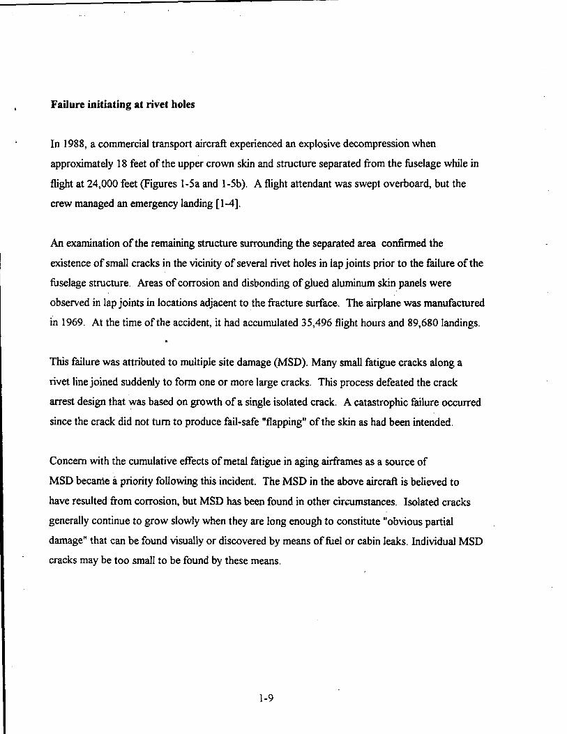
r Failure initiating at rivet holes

In 1988, a commercial transport aircraft experienced an explosive decompression when

approximately 18 feet of the upper crown skin and structure separated from the fbselage while in

flight at 24,000 feet (Figures 1-Sa and 1-5b). A flight attendant was swept overboard, but the

crew managed an emergency landing [ 1-41.

An examination of the remaining structure surrounding the separated area confirmed the

existence of small cracks in the vicinity of several rivet holes in lap joints prior to the failure of the

fbselage structure. Areas of corrosion and disbonding of glued aluminum skin panels were

observed in lap joints in locations adjacent to the fracture surface. The airplane was manufactured

in 1969. At the time of the accident, it had accumulated 35,496 flight hours and 89,680 landings. b

This failure was attributed to multiple site damage (MSD). Many small fatigue cracks along a

rivet line joined suddenly to form one or more large cracks. This process defeated the crack

arrest design that was based on growth of a single isolated crack. A catastrophic failure occurred

since the crack did not turn to produce fail-safe "flapping" of the skin as had been intended.

Concern with the cumulative effects of metal fatigue in aging airframes as a source of

MSD becanie a priority following this incident. The MSD in the above aircraft is believed to

have resulted from corrosion, but MSD has been found in other circumstances. Isolated cracks

generally continue to grow slowly when they are long enough to constitute "obvious partial

damage" that can be found visually or discovered by means of fuel or cabin leaks. Individual MSD

cracks may be too small to be found by these means. .

1-9

(a) General view, left side of forward fuselage.

(b) General view, right side of forward fuselage.

Figure 1-5. An aircraft fuselage failure.

[From T. Swift, FAA]

1-10

These three case histories mark the evolution of attitudes toward aircraft structural design

from one based on safe-life procedures to the correct emphasis on damage tolerance

evaluation. While no quantitative surveys of transport aircraft failures have concentrated

on this issue, there is considerable additional experience to support this change in attitude.

Several examples are summarized in the following paragraphs.

Hawker Siddley

In Argentina, a Hawker Siddley AVRO 748 suffered an in-flight separation of a wing due

to fatigue on April 14, 1976. This had been the first AVRO aircraft to be designed on

fail-safe principles where wing bending structure had been separated into multiple

elements. Previous AVRO designs, such as the Manchester and Lancaster bombers, had

been designed with all wing bending material concentrated in front and rear spar caps.

The change to fail-safe design concept in the 748 did not prevent catastrophic failure

which was precipitated by fatigue cracking at multiple uninspectable sites. The current

damage tolerance design philosophy includes in-service inspections specifically based on

expected crack growth scenarios.

m

Dan-Air

A Dan-Air aircraft horizontal stabilizer failure in Zambia (1 976) occurred after only 400

hours of flight following 800 hours of service to Pan American Airways. Stainless steel

skin had been installed to relieve a buffeting problem. As a result, a stress concentration

was created at the steeValuminum interface. While maintenance was performed 6 inches

from the location of the crack that precipitated the failure, there was no planned

inspection. The fail-safe design did not prevent a failure. This type of crack was found in

dozens of aircraft inspected after the accident.

1-1 1

Propeller blades

In one case, a propeller blade was thrown while flying at 20,000 feet with the cabin fully

pressurized. No damage tolerance had been incorporated in the design of this particular

aircraft. The cabin pressure of 4.6 psi (corresponding to a nominal skin stress, PWt = 13

ksi) produced 17 feet of damage to the fuselage. The crew of the aircraft managed a safe

landing. The fbselage material was 7075-T6 aluminum. This material has low fiacture

toughness, so it has little crack stopping ability and generally small critical crack lengths.

Passenger door comers.

All passenger aircraft have problems with the concentration of stress at details such as

doors and windows. In one case, an operator found a comer crack and repaired it. At

that time, the engineering involved was restricted to a static strength analysis of the repair;

fatigue was not considered. Such patches did not always fix the problem since they were

often too stiff and adversely affected the stress distribution local to the patch. This type of

detail has poor fatigue/damage tolerance.

The main problem posed by door comers is out-of-plane bending. The maximum principal

stress is at 45" across the detail. A subsequent finite element analysis of this configuration

predicted that the stress at the door comer was approximately 2.5 times the design stress.

1.2 RESULTS OF AIR FORCE SURVEY

Some sense of the sensitivity of structural elements to cracking problems and how often they

occur can be deduced from surveys conducted by the Air Force.'

Adchtional experience is also documented in Technical Report AFFDL-TR-79-3 118, Volume 111, titled Durabiliw 1

Methods Development - Structural Durabilitv Survey: State-of-the-Art Assessment.

1-12

Figure 1-6 shows the distribution and magnitude of service cracking problems in Air Force

I aircraft. There are a total of 3 1,429 major and minor cracking problems recorded on twelve

types of military aircraft. The distribution shows that the majority of incidents were in the

fixelage and wing with about the same number in each.

Figures 1-7(a) and (b) illustrate examples of two Air Force surveys of major cracking incidents.

During a 2 1 -month period, in one study (Figure 1 -7(a)), 1226 major crackindfdure incidents

were reported. The majority of these were fatigue initiated, with corrosion fatigue second,

followed by stress corrosion. In another study (Figure 1-7(b)), out of 64 major cracking incidents

reported, the majority were due to stress corrosion followed by corrosion fatigue and fatigue in

about equal numbers. It is noted that some failures were attributed to overload. This is rare in

commercial transport history.

Figure 1-8 shows the distribution of origins of those failures reported in Figure 1-7(b). The

majority of failures were due to poor quality where cracks initiated at holes. Material flaws,

defects, and scratches were second, followed by poor design details. This magnitude of cracking

incidents also contributed to an Air Force decision to change the design philosophy of their

structures. Prior to this time, the main philosophy had been a safe-life approach where the design

was based on a full scale fatigue test to four lifetimes.

1.3 COMl'ARISON OF OLD AND NEW APPROACHES

This section describes the elements of the older safe-life method (fatigue design) and contrasts it

with the concepts of fracture mechanics and crack propagation that are central to the current

damage tolerance approach. Even though the safe-life approach is not allowed as a basis for

certification of most major transport & m e components, AC 25.571-1 does permit exceptions

in certain cases, and in any case it is still important to understand the fatigue performance of

structure.

1-13

A

\

WINGS

\

EM PEN NAG E

FUSELAGES NACELLES & PYLONS

\ \ % LANDING

GEAR

Figure 1-6. Examples of distribution and magnitude of service cracking problems. b

UNKNOWN UNKNOWN

(a) 1226 major crackinglfailure incidents (b) 64 major crackinglfailure incidents

(21-month period) (Ref A h D L TR-70-149).

(Ref. USAF report on study of aircraft

structural integrity).

Figure 1-7. Crack initiatiodgrowth and failure mechanisms.

1-14

1.3.1 Fatigue SafeLife Approach

Metal fatigue was first recognized as an engineering problem over a century ago, when the

German railways encountered a series of axle failures which could not be explained fiom past

experience. The concept of fatigue as the result of repeated loading was proposed, and a

fatigue-resistant axle design was developed after several years of empirical study by means of full

scale axle fatigue tests [l-51. The relationship between fatigue and cyclic stress could be easily

visualized for axles, where the material was alternately subjected to tension and compression as

the axle rotated under the static loads imposed through its bearings. As a result, the rotating

bending fatigue test at laboratory scale became the standard in the field for more than half a

century (Figure 1-9), with the fatigue life defined as the number of cycles to specimen failure.2

The cyclic fatigue stress concept has since been extended to more complicated cases; early

ROTATl N G BENDING -

TEST /

STRESS

50% "S-N" CURVE

I I I I I I I I . I *

1 IO 100 l o 3 104 10' l o 6 10' 10' N

Figure 1-9. Results of a typical fatigue experiment.

~~~ ~

For typical laboratory size specimens, about 95% of this life is consumed by crack formation, and only 5% by 2

slow crack propagation.

1-16

developments are briefly summarized in Timoshenko's history [ 1-61, A good summary of recent

(circa 1950 to 1970) fatigue design practices is given by Osgood [ 1-71, and a detailed description

of European airframe fatigue design practices has been prepared by Barrois [ 1-81.

Basic material properties in fatigue can be summarized by an "S-N" curve and a modified

Goodman diagram. The S-N curve (Figure 1-9) is an empirical description of fatigue life based

on rotating bending or similar tests, where SA is the amplitude of the applied stress cycle and N is

the expected number of cycles to failure. The S-N curve describes the material behavior only

under the condition of zero mean stress. For design purposes, the material is tested over a range

of stresses corresponding to lives of one cycle at ultimate strengthf, to one equivalent to

unlimited duration at the endurance strength&.

There is actually no unique S-N curve for any material. If several nominally identical specimens

are tested at the same stress amplitude, the number of cycles to failure is generally different for

each specimen, as indicated by the open-circle symbols representing individual data points in

Figure 1-9. The shortest and longest individual life may differ by as much as a factor of 10 in

some cases. The data points at each stress amplitude are averaged to produce the 50th percentile

S-N curve shown in the figure.

As the tests are repeated at lower stress amplitude, the individual lives begin to spread out, and

"run-outs"'are obtained in some tests. A run-out is a specimen that has not failed after the longest

time one is willing to wait. In Figure 1-9, the run-outs are represented by solid circles with

arrows plotted at N = 2 xlO* cycles (the maximum waiting time in this case). As the stress

amplitude is fbrther decreased, the proportion of run-outs increases, and a material "endurance

strength" f, is sometimes defined as the stress amplitude where the run-out proportion reaches

100 percent. Fatigue life is sometimes said to be unlimited at stress arfiplitudes below f,, but,

strictly speaking, all one can say is that the life at these low stress amplitudes exceeds the test

time.

1-17

The effect of non-zero mean stress is schematically illustrated in Figure 1-10. Stresses in service

such as those resulting fiom aircraft maneuvers are cycles more complex than the ideal laboratory

pure alternating wave. The effect of mean stresses contained in these complex cycles shifts the

average lives fiom the values expected fiom S-N data. A modified Goodman diagram is used to

extend the description to cases in which the material is subjected to alternating stress

superimposed upon a mean stress. The usual presentation is in the nondimensional form shown in

Figure 1-1 1, where both the alternating stress amplitude SA and mean stress S, are expressed as

fractions of the material's ultimate static strengthf,. Both S-N curve data and experimentally

determined Goodman diagrams for aircraft structural alloys are well documented (see ref [l-91).

Figure 1 - 12 illustrates the Goodman diagram (using unscaled stresses) for 2024-T4 aluminum.

LAB~RATORY S A

AIRPLANE LOWER WING SKIN MANEUVER

Figure 1-10. Effect of mean stress.

1-18

0 0.5 1

Figure 1 - 1 1 . Modified Goodman diagram.

2024-T4,K = 4 t

GAG lo I

GUST 0

\o

10 MANEUVER

0

0 l . I . I . , , I 1 . 1

4 6 8 10 ' 12 14 0 2

Figure 1 - 12. Goodman diagram for 2024-T4 aluminum.

Source: ALCOA Structural Handbook.

1-19

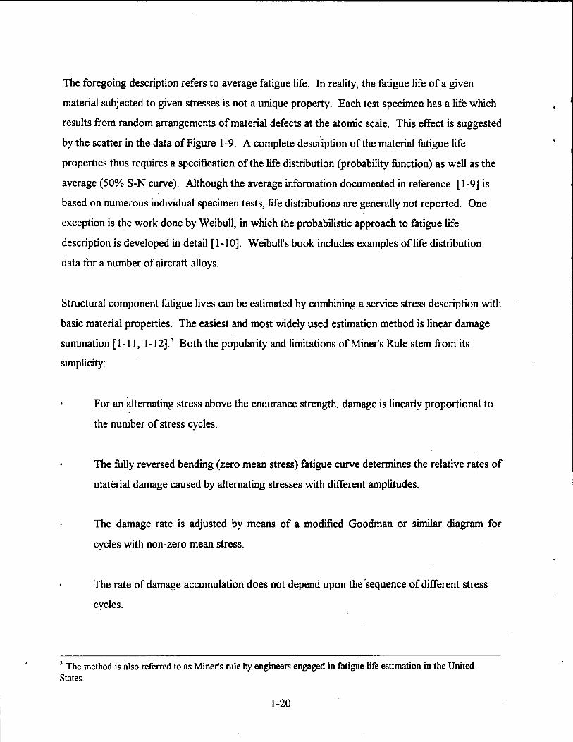
The foregoing description refers to average fatigue life. In reality, the fatigue life of a given

material subjected to given stresses is not a unique property. Each test specimen has a life which

results from random arrangements of material defects at the atomic scale. This effect is suggested

by the scatter in the data of Figure 1-9. A complete description of the material fatigue life

properties thus requires a specification of the life distribution (probability function) as well as the

average (50% S-N curve). Although the average information documented in reference [l-91 is

based on numerous individual specimen tests, life distributions are generally not reported. One

exception is the work done by Weibull, in which the probabilistic approach to fatigue life

description is developed in detail [ 1-10]. Weibull's book includes examples of life distribution

data for a number of aircraR alloys.

Structural component fatigue lives can be estimated by combining a service stress description with

basic material properties. The easiest and most widely used estimation method is linear damage

summation [l-11, 1-12].' Both the popularity and limitations of Miner's Rule stem from its

simplicity:

For an alternating stress above the endurance strength, damage is linearly proportional to

the number of stress cycles.

The hlly reversed bending (zero mean stress) fatigue curve determines the relative rates of

material damage caused by alternating stresses with different amplitudes.

The damage rate is adjusted by means of a modified Goodman or similar diagram for

cycles with non-zero mean stress.

The rate of damage accumulation does not depend upon the 'sequence of different stress

cycles.

The method is also referred to as Miner's rule by engineers engaged in fatigue life estimation in the United 3

States.

1-20

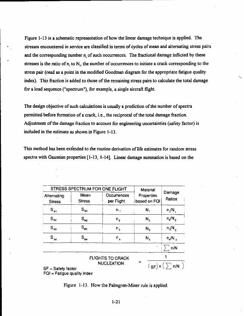
Figure 1-13 is a schematic representation of how the linear damage technique is applied. The I stresses encountered in service are classified in terms of cycles of mean and alternating stress pairs

and the corresponding number n, of such occurrences. The fiactional damage inflicted by these

stresses is the ratio of ni to N,, the number of occurrences to initiate a crack corresponding to the

stress pair (read as a point in the modified Goodman diagram for the appropriate fatigue quality \

index). This fraction is added to those of the remaining stress pairs to calculate the total damage

for a load sequence ("spectrum"), for example, a single aircraft flight.

The design objective of such calculations is usually a prediction of the number of spectra

permitted before formation of a crack, i.e., the reciprocal of the total damage fraction.

Adjustment of the damage fraction to account for engineering uncertainties (safety factor) is

included in the estimate as shown in Figure 1-13.

This method has been extknded to the routine derivation of life estimates for random stress

spectra with Gaussian properties [l-13, 1-14]. Linear damage summation is based on the

STRESS SPECTRUM FOR ONE FLIGHT

Stress Stress per Flight 1 based on FQI

Material Damage Ratios I

FQI = Fatigue quality index

Figure 1 - 13. How the Palmgren-Miner rule is applied.

1-21

assumptions that each stress cycle affects the material independently, and that the spectrum at a

stress raiser is linearly scaled fiom the nominal stress spectrum. Neither assumption is true in

most service situations, however. Even laboratory experiments have shown that actual life can be

changed simply by rearranging the order of stress cycles in the spectrum, or that life estimates

scaled from nominal stresses do not agree with the experimental results when the test specimen

contains a notch or a hole [ 1-15].

Simulated service testing or field experience is required to obtain an accurate estimate of the life

distribution. When similar structural details are employed in evolving designs (e.g., the evolution

of transport airflames in an individual manufacturer's product line), the results of tests and field

experience are usually fed back to adjust the estimation procedure. Most such adjustments are in

the form of a fatigue quality index (FQI) and factor of safety or the use of an S-N curve more

conservative than the average, although in some cases aerospace companies have developed

elaborate empirical nonlihear damage summation procedures to replace Miner's rule. Such special

procedures may be well calibrated for details similar to that fiom which they were derived, but

extrapolation to other details can generally be expected to give poor results.

The FQI is used to account for the effects of local stress, by reference to S-N curves obtained

fiom specimens with standard notches. Each such specimen has a known elastic stress

concentration factor, Kt, at the root of the notch, as determined by the notch geometry. Since

these spechens fail at the notch root, a plot on a scale of the nominal stress amplitude SA is considered to characterize the S-N curve for the stress concentration factor K,. (Notched-

specimen S-N curves are generally obtained for K, = 2,3,4, and 5.)

Figure 1-14 outlines how the FQI is derived from notched-specimen S-N curves. The schematic

represents two replicas of a double-shear connection detail which is being tested in fatigue. The

data points, which represent the results of these tests, are compared graphically with the family of

notched-specimen S-N curves for the material. In general, the detail will not precisely follow any

one S-N curve, but an "effective" K, for the range of stress amplitudes expected in service can be

estimated fiom the comparison.

1-22

Similar comparisons of data fiom a fill scale fatigue test of an airframe provide eff'ective Kt values

for typical fastener details. These values are referred to as fatigue quality indices because they

reflect the effects of detail design and fabrication quality, as well as geometric stress

concentration. For example, Kt = 3 for the stress at the edge of an open circular hole in a skin

under tension, but the FQI ranges from 3.5 to 4.5 for filled fastener holes in typical transport

airframe details.

BASE MATERIAL 0 0 - WITH NOTCH w

N

FQI = 3.5 to 4.5 for typical airframe fastener details

. - Figure 1-14. Fatigue quality index.

The FQI accounts for what is known about the average effect of fatigue when combined with

realistic quality. A factor of saf'ety (sometimes also called a "scatter factor") is applied to

estimates of average fatigue life to account for the uncertainties. These include the previously

mentioned random effects of material behavior and differences of amid service loads fiom the

loads assumed for the purpose of estimating fatigue life (Figure 1-15). Fatigue factors of safety

Erom 3 to 5 (but in some cases as high as 8) have historically been used to estimate airframe safe

life.

1-23

MATE RIAL "S C ATT E R 8

t

When the FQI and factor of safety are properly applied, the calculated safe-life is usually a

conservative estimate of the airfiame's useful economic life. What this means is that, within the

safe-life, most of the details in the airframe will not have had enough time to form cracks. If the

safe-life is exceeded, the rate of crack formation can be expected to rise, and (usually well before

the unfactored 50th percentile lifetime) enough cracks will be present to make repair

LOAD INTERACTION EFFECTS b S S S

1 HIGH- LO^ 1 RANDOM\ I . I 0 1 l 0 I c

T T T INCREASING FATIGUE LIFE -

Figure 1-1 5 . Uncertainties addressed by safety factor.

uneconomical. A full-scale fatigue test of a transport airfiame prototype is generally conducted to

one or two expected service lifetimes for the purpose of veriijmg that the design meets its useful

economic life goal.

Recently, some older airframes have been reexamined to more closeiy estimate useful economic

life. This is done, as a part of the continuing airworthiness program, by ground testing a retired

high-the airfiame which has reached or exceeded the original economic life goal.

1-24

1.3.2 Damage Tolerance Assessment (DTA) Approach 1

The case histories presented in Section 1 . 1 show why in modem structural design attention is

focused on crack propagation life. Originally, the term damage tolerance meant the ability to

endure sudden damage, for example, penetration of a hselage by a propeller blade without

catastrophic failure. It has come to mean setting life limits, i.e., inspection intervals that are based

on the time for a crack to lengthen or propagate.

The epitome of a damage tolerance problem is illustrated by the failure of the front lower spar cap

of a DC-8-62. A crack in a stiffening element was revealed by a fuel leak observed after 32,000

hours of service. Examination of the failed region gave a clear impression of the process. A

count of the striations in the fracture surface indicated the effect of each cycle of loading on the

growth of the flaw, from a small crack to a length large enough to allow fuel to escape. Such a

pattern is a signature that C a n be used as forensic evidence to trace size of the crack very nearly

on a flight by flight time scale.

This case illustrates the importance of three interconnected notions that are the central elements

ofFAR 25.571.

Crack propagation: A.crack in a structure will increase in size in response to application

of cyclic-loads. As shown schematically in Figure 1-16, growth is neglrgible when the crack

is very small. Since these effects are nearly impossible to observe, it can be argued that

some tiny flaws are always present in a structure. An alternative interpretation is that a

small crack is initiated in perhaps 5% of the time range of the diagram due to a

manufacturing flaw or material inclusion and then grows during the greater part of the time

range to failure. As the crack increases in size, increments of extension get larger until a

critical dimension is attained at which the structure fractures in the course of a single cycle

of loading.

1-25

<

LIMIT LOAD I

1

- I CRACKGRbVlH I LIFE

Y 0 < 0 a

- -m FLIGHTS

_-

Figure 1-16. Crack growth in response to cyclic loads.

Residual strength: The level of stress that will induce rapid fracture is sensitive to the size

of a crack in a stbcture. Figure 1-17 is a schematic illustration of the inverse relationship

of critical stress and crack length. A structure with a history of few cycles of loading and a

short crack length has the capacity to resist fracture. This is indicated in the diagram by the

vertical distance between a level of service stress (dotted line) and the critical stress-crack

length curve. As fatigue loads accumulate, the crack lengthens, reducing the stress level

. - v) \ AXlMUM STRESS 3

I

CRACK LENGTH

Figure 1-17. Schematic relationship of allowable stress versus crack length.

1-26

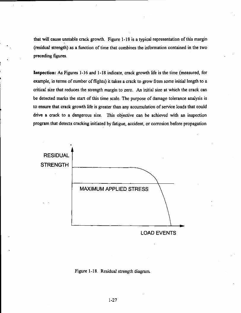
that will cause unstable crack growth. Figure 1-18 is a typical representation of this margin

(residual strength) as a function of time that combines the information contained in the two

preceding figures.

Inspection: As Figures 1-16 and 1-18 indicate, crack growth life is the time (measured, for

example, in terms of number of flights) it takes a crack to grow from some initial length to a

critical size that reduces the strength margin to zero. An initial size at which the crack can

be detected marks the start of this time scale. The purpose of damage tolerance analysis is

to ensure that crack growth life is greater than any accumulation of service loads that could

drive a crack to a dangerous size. This objective can be achieved with an inspection

program that detects cracking initiated by fatigue, accident, or corrosion before propagation

b

t RESIDUAL

\

MAXIMUM APPLIED STRESS

LOAD EVENTS

Figure 1-18. Residual strength diagram

1-27

to failure. Inspection frequencies must be at intervals that are fractions of expected growth

life to afford the opportunity for corrective action that maintains structural safety if cracks

are found. The economic feasibility of an inspection plan must consider the cost trade-off

between inspection methods and intervals. As Figure 1-16 suggests, crack growth life for

small cracks detected using an expensive nondestructive inspection (NDI) procedure will be

longer than the interval corresponding to larger crack sizes that are found with less

expensive visual inspection.

A sound knowledge of the principles of fracture mechanics is needed to perform the damage

tolerance evaluation required by Part 25 of the FAA regulations. With this objective in mind, this

handbook has been planned with a view to providing FAA engineers with appropriate background

in order that they may improve their ability to review manufacturers' data.

Fracture mechanics ca i be looked upon from a metallurgical viewpoint or a stress analysis

oriented viewpoint. The former usually takes place after failure with fiactographic analysis of the

fracture surface, for example. The latter is primarily associated with the calculation of crack

growth life and- residual strength in order to establish an inspection program to prevent failure.

Since the FAA is involved in reviewing damage tolerance evaluations to prevent failures, it is

appropriate here to concentrate on the stress analysis oriented fracture mechanics approach. .

. - The concepts of damage tolerance have been organized into three areas. Chapter 2 begins with a

description of the fbndamentals of crack behavior. The roles played by stress history, crack

geometry, and material properties in residual strength assessment are defined and placed in

context. The relation of these factors to crack growth is the foundation of DTA.

Chapter 3 is devoted to interpretation of measurements of crack length under cyclic loading. Data

for fatigue crack propagation are rigorous and repeatable, not as scattered as S-N curves that are

based on a concept as imprecise as crack initiation. However, characterization of crack

propagation rates is still largely empirical; laboratory experiments are necessary to determine how

cracks actually grow. In addition, data correlation procedures must be applied to account for

1-28

circumstances of service that are distinct from the experimental conditions. The dependence on

such empiricism to develop a crack growth curve for a specific structural element emphasizes the

need for continual experimental confirmation of DTA in the design process.

These notions are brought together in Chapter 4 from the point of view of assessing an airframe.

Step-by-step procedures and examples are presented to illustrate proper paths for design reviews.

1-29

REFERENCES FOR CHAPTER 1

1-1. Damage Tolerance and Fatigue Evaluation of Structure, FAR 25.571. 1-2. Damage Tolerance and Fatigue Evaluation of Structure, Federal Aviation

1-3. Airplane Damape Tolerance Requirements, MIL-A-83444 (USAF), 1974. Also, &

1-4. Arcraft Accident Reuort - Aloha Airlines, Flight 243. Boeing 737-200, N73711, Near

1-5. Wohler, A.., Zeitschrift &r Bauwesen, &, 641-652 (1858); 10. 583-616 (1860); l6, 67-84

1-6. Timoshenko, S.P., History of Strength of Materials, McGraw-Hill, New York, 1953. 1-7. Osgood, C.C., Fatigue Design, Wiley, New York, 1970. 1-8. Barrois, W.G., Manual on Fatigue of Structures, NATO Advisory Group for Aerospace

1-9. Metallic Materials and Elements for Flight Vehicle Structure, MIL-HDBK-5E (USAF)

1-10. Weibull, W., Fatigue Testing and Analvsis of Results, Pergamon Press, New York, 1961. 1 - 1 1. Palmgren, A,, "Die Lebensdauer von Kugellagern," Zeitschrift des Verein Deutscher

1-12. Miner, M.A., "Cumulative Damage in Fatigue," Journal of Applied Mechanics 12.

1-13. Bums, P.M.and Bender, M.A., Aircraft Load Alleviation and Mode Stabilization ( L A M S ) ,

1-14. Crandall, S.H.and Mark, W.D., Random Vibration in Mechanical Systems, Academic

1-15. Schijve, J., The Accumulation of Fatime Damage in Aircraft Materials and Structures,

Administration, AC 25.571-1 (1978).

Force h i d e Specification, AFGS-872214 June 8, 1990.

Maui, Hawaii, April 28, 1988. NTSB/AAR-89/03.

(1866); 20, 73-106 (1870).

Research and Development, AFARD-MAN-8-70, June 1970.

June 1987. 0

Ingenieure 68, 339-341 (1924).

A1 59-A164 (1 945).

The Boeing Company and Honeywell, Inc., AFFDL-TR-68-158, 1969.

Press, New York, 1973.

NATO Advisory Group for Research and Development, AGARD-AG- 157, January 1972.

1-30

CHAPTER 2:

FRACTURE MECHANICS

2. FR4cmMEcHANIcs

Fracture mechanics is an outgrowth of the field of strength of materials. Early work on the

strength of materials focused first on basic properties and later, as the theories of elasticity and

plasticity were developed, on the strength of structures or components containing known stress

raisers [2-11. Fracture mechanics deals with the strengths of materials and structures which

contain flaws in the form of detectable or visible sharp cracks.

2.1 STRESS CONCENTRATION, FRACTURE AND GRWFTI'H THEORY

Many structures have discontinuities such as holes and notches. Often these discontinuities

produce local elevation of stress in comparison to the applied stress. The resulting stress

concentration is defined as the ratio of the local elevated stress to the applied nominal stress.

. Stress concentration factors can be derived by applying the theory of elasticity to specific

problems. Two problems of great historical and practical importance are the circular hole and the

elliptical hole. The circular hole is shown in Figure 2-1 for a uniform stress, S, in the y-direction.

A plate without a hole produces a uniform stress, S, throughout the plate, while at the highly

stressed points A and B at the hole, the normal stress rises to 3s. Thus the circular hole in a large

plate has a stress concentration factor of 3, which is independent of the hole radius. The elliptical

hole in a 13rge plate is shown in Figure 2-2. The analysis by Inglis [2-21 produces a stress

concentration factor kr = (1 + 2a/b), where a and b refer to the semi-major and -minor axes,

respectively. Since the radius of curvature at the ,end of the major axis of an ellipse is p = b2/u, the stress concentration factor can be rewritten as

or k, = 1 + 2Q b

2- 1

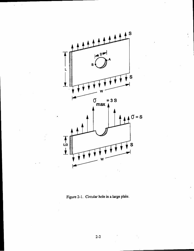
= S

Figure 2-1. Circular hole in a large plate.

2-2

= s

at A, B:

Figure 2-2. Elliptical hole in a large plate.

2-3

which is dependent on the geometry of the ellipse. For the limit of a circular hole, p = a and k, = 3 . If we model a sharp crack as an ellipse for which p -+ 0 then kr + m and an infinite stress is predicted, which implies that a structure with a crack of any size will immediately fail!

However, we know fiom experience that practical structural systems such as airplanes,

automobiles, and railroad cars and tracks, have a multitude of cracks and defects, yet they very

rarely fail in use.

It is reported [2-3 J that Inglis was not welcomed at professional engineering society meetings for

some years after his paper was published. Contemporary engineers certainly would have had no

difficulty in recognizing the fact that most structures continued to stand, in defiance of the new

theory, and they should have looked forward to challenging the theoretician. Perhaps they felt

uncomfortable with a stress concentration factor, apparently supported by the principles of

mathematics, but which increased without limit unless one was willing to fearlessly set an arbitrary

minimum on the elusive crack tip radius, p. To take such a step in an affair concerning safe design practice, with no supporting data, is something most engineers would be reluctant to do.

It later turned out that the engineers' discomfort was well founded. The stress concentration

factor could not be used reliably for crack problems. A different approach was needed. The first

step in the new direction was taken in 1920 by Griffith 12-41, who based his approach on an

energy balance analysis supported by experimental data.

Grifith introduced the idea of a sharp crack as a strength-limiting flaw fiom the results of a series

of experiments on glass rods. It is of historical interest to note that Griffith worked for the Royal

Aircraft Establishment in England, and one of his reasons for examining glass rods was to study

failures in glass windshields on airplanes. He measured the breaking strengths of glass rods which

were of the same diameter and original length, and he found a wide,variation in their strengths.

He then continued the experiment on the broken halves of the original rods, on the halves of the

halves, and so forth, finding that the average breaking strength increased in each trial. He

explained the results by postulating that glass contains surface cracks with randomly distributed

sizes, and that the largest crack in a given specimen determines the strength of the specimen.

2-4

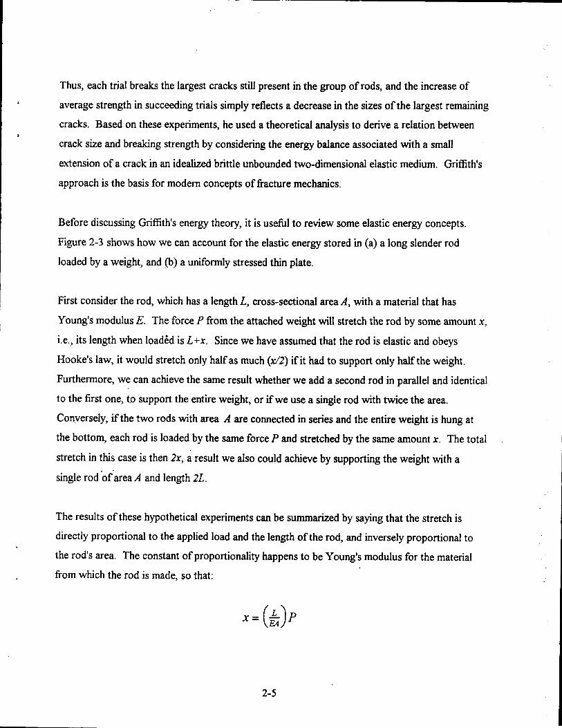
Thus, each trial breaks the largest cracks still present in the group of rods, and the increase of

average strength in succeeding trials simply reflects a decrease in the sizes of the largest remaining

cracks. Based on these experiments, he used a theoretical analysis to derive a relation between

crack size and breaking strength by considering the energy balance associated with a small

extension of a crack in an idealized brittle unbounded two-dimensional elastic medium. Griffith's

approach is the basis for modem concepts of fracture mechanics.

Before discussing Griffith's energy theory, it is usefid to review some elastic energy concepts.

Figure 2-3 shows how we can account for the elastic energy stored in (a) a long slender rod

loaded by a weight, and (b) a uniformly stressed thin plate.

First consider the rod, which has a length L, cross-sectional area A , with a material that has

Young's modulus E. The force P from the attached weight will stretch the rod by some amount x,

i.e., its length when load6d is L+x. Since we have assumed that the rod is elastic and obeys

Hooke's law, it would stretch only half as much ( d 2 ) if it had to support only halfthe weight.

Furthermore, we can achieve the same result whether we add a second rod in parallel and identical

to the first one, to support the entire weight, or if we use a single rod with twice the area.

Conversely, if the two rods with area A are connected in series and the entire weight is hung at

the bottom, each rod is loaded by the same force P and stretched by the same amount x. The total

stretch in this case is then 2x, a result we also could achieve by supporting the weight with a

single rod 'ofarea A and length 2L.

The results of these hypothetical experiments can be summarized by saying that the stretch is

directly proportional to the applied load and the length of the rod, and inversely proportional to

the rod's area. The constant of proportionality happens to be Young's modulus for the material

from which the rod is made, so that:

2-5

I Load P

" A

Displacement

1 1 2 2 Strain energy = -Px = -kx2

(a) Slender rod.

b

t Q = PA; Volume V = AL

1 1 2 2 Strain energy = -mV = -a2VIE

Strain, €

(b) Uniformly stressed thin plate.

Figure 2-3. Energy principles.

2-6

which can be rewritten as

where the quantity k = EAIL is called the s t f iess of the rod. The equation P = kx is represented by the straight line with slope k on the graph at the right of Figure 2-3(a).

Another way to interpret this equation is to consider the work done on the rod by the applied load

as it simultaneously increases and moves through a distance equal to the stretch. Since the load is

proportional to the stretch, the work done is represented by the shaded area under the line, or:

Work = -Px 1 = -kc2 1 2 2

This work is s xed in the&rod as internal energy, which can be thought of as a reservoir availa-le

to do work elsewhere when it is released.

The thin plate shown in Figure 2-3(b) behaves in the same manner, i.e., it possesses a stif€ness,

k = E A L d e t e h e d by its cross-sectional area, length, and Young's modulus. The expression of

Hooke's law for the plate can also be rearranged in the form:

or

This last equation is just the expression of Hooke's law for the material, in terms of the stress

o = PIA and strain E = x/L. It is also informative to remange the worWenergy expression:

1 1 2 2 Work(energy) = -Px = -(Ao)(LE)

or

Work (energy) = (&E) (AL)

2-7

The quantity AL is just the total volume of the plate, and thus we can think of energy stored per unit volume. Substitution of Hooke's law provides the equivalent expressions:

as the work or

o2 1 1 2 2 E 2 - -E&' -O& = - -

for this quantity, which is usually referred to as strain energy or strain energy density.

W t h analyzed a system similar to the previously mentioned uniformly stressed plate, but

considered the plate to have a me-existing crack of length 2a as shown in Figure 2-4(a), with the

corresponding load-displacement curve up to load P and displacement x. (The displacement x

refers to the displacement of the load application points, as for example at the grips of a tensile

testing machine.) He then analyzed the change in energy of the system if the crack were to grow

by a small amount 2Aa with the load application points remaining fixed, i.e., the displacement x not changing. As the Hack length increases, the plate becomes less stiff (more flexibIe) and the

slope of the load displacement curve decreases as shown in Figure 2-4(b). The applied load for

the case of a crack of length 2(a + Aa) then decreases from P to P-AP. The change in energy storage in the kystem, the strain energy decrease, is the difference in the two shaded energy

storage triangles in Figure 2-4.

Griffith postulated that this release of elastic energy is used to overcome the resistance to crack

growth. ,The resistance is a consequence of the surface energy required to break interatomic

bonds and form the new crack surface, represented by 2Aa. He reasoned that in order for a crack to elongate, the

than) the

of strain energy release with crack extension must be equal to (or greater

of energy absorption required to overcome the resistance to crack growth.

2-8

rea A'

, Load EB'c K ' c r EA L

X Displacement

Stored energy = -Px 1 2

(a) h t i a l crack length 2a

Load drops as crack extends (constant x) p - - - - - - - - - - - - - - t Load 0

- - - - - -.---

rea A"

Displacement X

Stored energy = -(P 1 - d p ) x 2

b) Elongated crack length 2(a + Aa)

Figure 2-4. Energy principles for cracked plate.

2-9

Griffith used this energy principle to produce the following simple relation governing the onset of

crack propagation &om an existing crack:

acfi = constant (2-2)

where ac is the critical stress, a is half the original crack length, and the constant is a material property depending on the material surface energy and elastic modulus. Equation (2-2) indicates

that crack extension occurs in an ideally brittle material when af i reaches a constant critical value for a given material.

It is important to also consider the possibility that the boundaries of the structure can supply

additional energy to make the crack propagate. For example, the flexibility of the testing machine

could add system energy to the crack extension. Therefore, the testing machine should be much

stiffer than the cracked plate being tested. In the hselage of an aircraft, the pressurized air is also

a source of additional energy. b

The idea behind the energy balance can be explained in a simple and direct manner. E a crack in a

body is imagined to extend, then the sum of energy remaining in the body after extension, work

done on the body during the extension, and energy dissipated into irreversible processes occumng

during the extension should equal the energy which was stored in the body before the extension.

This is nothing more than a restatement of the hndamental physics principle that work and energy

are equivalent, and that energy cannot be created or destroyed.

A convenient feature of the energy approach to problems in stress analysis is that we can take

great liberties with the assumptions we make to define the problem. Taking such liberties may

produce a solution in error by a large numerical factor, but the basic relationships between key

variables are preserved. For example, consider the extension of the crack in the plate depicted in

Figure 2-4. In order to simplie the analysis, we shall make the following assumption about the

stress distribution in the cracked plate (see Figure 2-5).

2-10

V A

-X

Figure 2-5. Plate with a center crack.

Draw a circle on the plate with the crack as its diameter. Assume that the stress a, is equal to

the applied stress o everywhere in the plate outside the circle, that o, = 0 everywhere inside the circle, and that

correct, since we expect stresses ox, o,, and T~ to exist near the crack, the wumption quickly leads to a useful result when it is used in an energy analysis.

the other stress components are zero everywhere. Although this is not quite

Let Ul be the strain energy stored in the plate in its initial state, when the crack length is 2a. In an

earlier example, we saw that the strain energy density in material uniformly stressed by ov = a could be expressed as a2/2E. The total energy is then the product of this density and the volume of the plate, less the volume in the unstressed circle:

.

2-1 1

Now consider what happens when the crack is imagined to extend to the length 2(a +Aa), where

the extension 2Aa is assumed to be extremely small compared to the original crack length 2a, while the applied stress is assumed to remain constant. This last assumption corresponds to an

experiment in which the plate is loaded by a dead weight, rather than by a testing machine with

grips kept in a fixed position. In a real experiment, the dead weight would move, stretching the

more flexible plate and thus doing work on it. Conversely, another curious and unrealistic property of the assumed stress distribution is that the strain E,, = o/E remains constant, the plate does not stretch, and the weight remains stationary and does no work.

However, the energy U, stored in the plate after the crack extension is less than the original

energy U,. This follows directly from a consistent application of the stress distribution

assumption:

The elastic energy released by the crack extension is then:

xo2atAa E u, - u2 = d[2mtAa + xt(Aa)2] E

2E

since the small quantity X(ALZ)~ can be neglected in comparison to 2mAa.

It is more convenient to express the last result as the rate of energy released per unit of new crack

surface area. The new area is 2rAa. The energy release rate p2r unit of new crack area (defined by the symbol G) is thus given by:

UI - UZ - - - xo2a 2tAa - 2E G =

How are the new surfaces created? Evidently, the bonds between atoms lying on either side of a

line extended from the crack tips must be broken, and energy is required to do this. Since the

material is assumed to be homogeneous, we can postulate that the energy dissipated in the

bond-breaking process, per unit of new surface area, is a constant property of the material. For

historical reasons, physicists have always counted the upper and lower surfaces of a crack as

2-12

separate areas, and the dissipation rate ye was defined accordingly. Thus, the energy account for

the crack extension is represented by G - ye. We can now argue, as Griffith did, that the

balance of G - 2ye determines whether the crack will actually extend or not. If G is less that 2ye, then more energy is needed to create the new surface than is released fiom the elastic storehouse,

and the crack will not extend. Conversely, if G is greater than 2ye, the crack will extend

spontaneously, and the difference G - 2ye will be dissipated in other ways (vibration and heating of the plate, sound, etc.).

The crack will also extend spontaneously if just enough energy is released, i.e., if G = 2y, Substituting the expression previously derived for G and rearranging then leads to:

Thus, we have derived frcm basic physical principles the result that the strength of a cracked body is determined by a relationship of the form oJsr = constant.

Griffith’s analysis was similar but was based on the accurately derived Inglis solution [2-21 for the

stress around an elliptical hole. Consequently, Griffith was able to find the correct numerical

results:

In 1957, Irwin [2-51 reexamined the problem of the stress distribution around a crack. He used

advanced mathematical methods to directly model a medium containing an idealized sharp cut,

thus eliminating the crack-tip radius which had made the Inglis ellipse Solution so controversial.

In order to understand the character of Irwin’s solution, consider again the thin plate with a

central crack of length 2a and uniform tension ov = a applied to the ends. We now focus our

attention on a small area near one end of the crack, where polar coordinates (r, e) are centered at

2-13

the crack tip (Figure 2-6). Very close to the crack tip (r (( a), Irwin's stresses are dominated by

the terms:

Kr cos- 1 - sin-sin3- 6 2 e[ e 2 "I 2 0 x = -

0, = -

8 . 8 e cos - sin -cos 3- 2 Tqy = - KI JG 2 2

where K, is a scaling factor and z indicates out-of-plane direction. The stresses all increase without limit as the crack tip is approached (r + 0), i.e., they behave in the way that Inglrs predicted by modeling a crack as the limiting case of an elliptical hole. Thus, neither solution can

be used to define a s t r k concentration factor. However, Irwin's scaling factor KI does define the

rate of stress concentration and thus provides a way to compare different situations. KI is called a stress intensity factor to reflect its rate-measuring character and distinguish it from the stress

concentration factors.

tit ttt tit tt t t CT X

Figure 2-6. Stress components in Irwin's analysis.

2-14 .

For the case of a crack length much smaller than the length and width of the plate, Irwin found

that Kl = o,/Z (2-5)

He thus established a connection between the stress intensity factor and Griffith's energy release concept, namely, that the combination CT ,/Z is the essential factor which determines the strength of a cracked body. Repeating Griffith's analysis of an imaginary crack extension, he showed that

the stress intensity factor was related to the energy release rate by the formula:

K: G = - plane stress E '

for thin plates.

Griffith's analysis led to a criterion that the strength of a cracked body is determined by G = G,,

where G, is a material property. It then follows that an equivalent criterion can be based on the

stress intensity factor:

Kl =K, (2-7)

where Kc is a critical value based on material, loading, and geometry. In other words, a crack will

propagate when the stress intensity factor reaches the critical value K,.

Irwin also considered the case of a body for which the lateral dimensions are very small compared

to the thickness. The limiting case for such thick bodies is plane strain condition. The front and

back lateral surfaces of the body are assumed to be rigidly restrained against expansion or

contraction in the through-thickness (z) direction. As a result, the strain E~ is zero and the effect

of Poisson's ratio induces a through-thickness stress 0 2 = v(o, + CT,) when the body is loaded

by stresses oxand a,, even though these stresses are uniformly distributed through the thickness. Irwin's plane strain solution for the cracked plate discussed earlier has the same local stress terms

as those given in equations ( 2 4 , but contains the additional through-thickness stress:

2-15

e oz = v(ox + oy) = - v cos - J G 2

In the case of plane strain, the relation between the stress intensity factor and the energy release

rate is changed to: K2 (' - ) I , plane strain E G = (2-9)

The elastic stress intensity factor has become one of the most commonly used means of translating

material properties into structural behavior. Stress intensity factor solutions for numerous

configurations of cracks in standard laboratory test specimens and cracks near typical structural

details are now available in several handbooks [2-6 to 2-91. Results are typically presented in the

form K, = p o f i (2- 10)

where p is a hnction df crack length and key structural dimensions such as plate width. Formulae for stress intensity factor are determined fiom analytic procedures (stress analysis) or

experimental techniques (photoelasticity). Some typical examples of center- and edge-cracked

plates are shown in Figure 2-7. Additional examples are contained in Appendix A. The material

between the crack tip and the edge of the plate is commonly called a ligament. For the

edge-cracked plate shown in Figure 2-7(b), the ligament width is (W- a).

The following simple example based on Figure 2-7 illustrates how the stress intensity factor

concept is applied to find critical crack length. Suppose that a i 0-inch wide plate is found to

contain an edge crack 2 inches long. The plate is 1/4 inch thick and has a yield strength Y = 39

ksi. Its design limit load is 65,000 pounds, based on 2/3 of the material yield strength. Would the

cracked plate be able to support its design limit load?

A laboratory test is conducted on a smaller specimen of the same material and thickness. The test

specimen is 2 inches wide and contains a central crack 1 inch long. The test specimen fractures at

a load of 10,000 pounds.

2-16

The formula from Figure 2-7(a) is first applied to find the material fracture toughness.

From the laboratory test

--- - 20, OOOpsi = 20 ksi 10 000 10,000 c c = - - wt 219.25

a = 0.5 inch

, - K, = j30,Ei

I a(;) = [set$ Kr - o f i for large W

(a) Plate with center crack under tension

- --

*a*

p($) = 1.12 - 0.231($) + 10.55($) 2

-21.72(g) 3 + 30.39($) 4

W '

(b) Plate with edge crack under tension.

Figure 2-7. Stress intensity factor formulae for some common geometries.

2-17

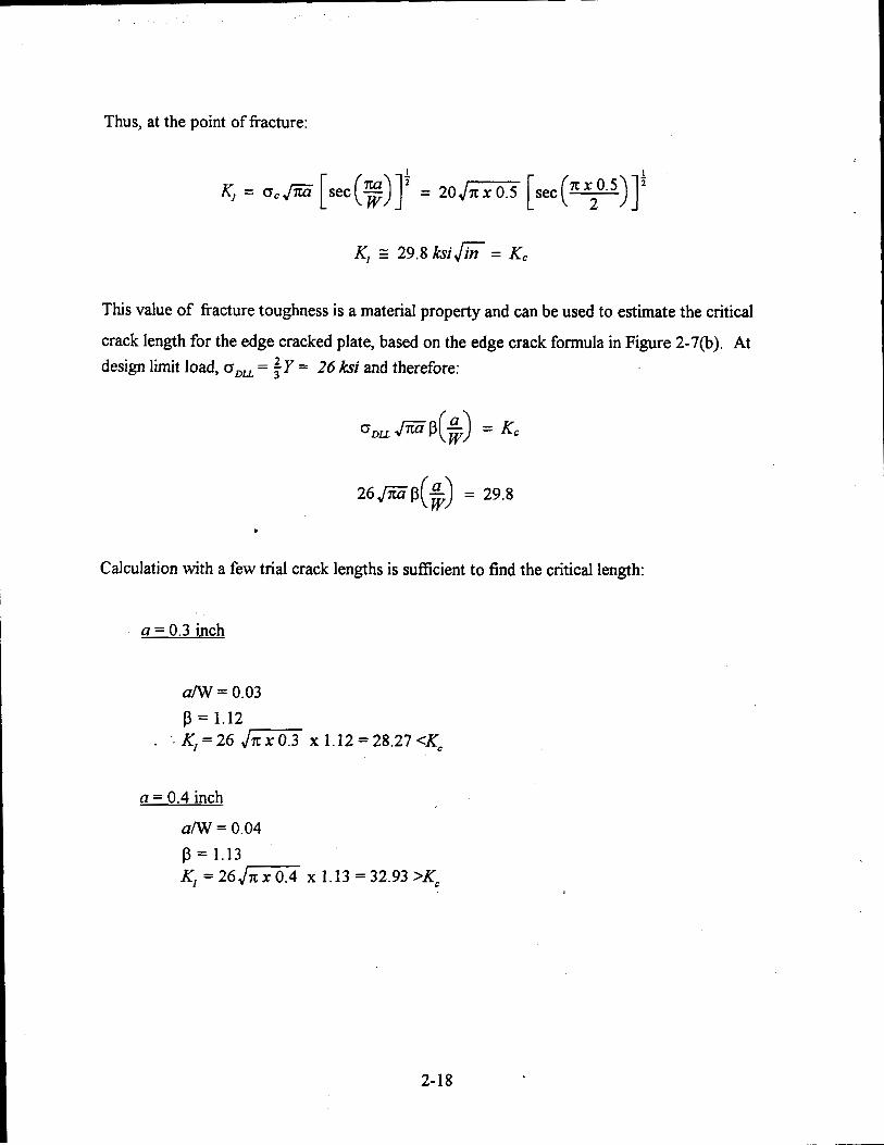
Thus, at the point of fracture:

I

4 = o,,tiiii [sec(:)Ii = 20 JEE [ s e c ( Y ) ] '

Kl E 29.8 h i 6 = K,

This value of fracture toughness is a material property and can be used to estimate the critical

crack length for the edge cracked plate, based on the edge crack formula in Figure 2-7@). At design limit load, oDU = f Y = 26 hi and therefore:

Calculation with a few trial crack lengths is sufficient to find the critical length:

a = 0.3 inch

alw = 0.03 p = 1.12

. .- K,=26 ,I= x 1.12=28.27<Kc

a = 0.4 inch

alw = 0.04 p = 1.13 Kl = 264- x 1.13 = 32.93 >Kc

2-18

From linear interpolation:

a, = 0.33 inch

alw = 0.033

K, = 26 ,/= x 1.12 = 29.75 z Kc p = 1.12

Based on the results of the small specimen test, the critical crack length for the 10-inch wide panel

at design limit load is about 113 inch. Thus, not only would the panel with the 2-inch edge crack

be unable to support the limit load, but also one would want to inspect other such panels quite

careklly because of the short critical crack length.

2.1.1 Fracture Modes b

The subscript "I" in the stress intensity factor K,denotes the fact that K, is associated with loads

that apply tension across the crack and thus tend to open it. This type of loading is referred to as

Mode I or the opening mode. Irwin also recognized the possibility that a crack might not be

oriented directly across a tensile load, and he defined two other modes corresponding to shear

loading. In one, the crack surfaces slide over each other perpendicular to the crack front (Mode

II). In the other, the sliding is parallel to the crack fiont (Mode m). Mode III is usually called

"tearing." The crack-tip stress intensity factors associated with the three modes are denoted by

K,, K,,, and Kru. Figure 2-8 illustrates the actions of the three basic loading modes.

. -

Tension at any angle to the crack surface can always be resolved into equivalent components of

tension across the surface, shear across the crack front, and shear parallel to the crack front.

2-19

Mode I Mode 11 Mode 111

Opening Shear Tearing

Figure 2-8. Fracture modes

e

Thus, any case of interest can be completely described by three stress intensity factors, one for

each basic mode. The near tip stress field for Mode I was given in equation (2-4). For Mode 11,

the dominant terms near the crack tip are:

crx = - -sin- 2 + cos-cos3- f i 2 Krr e[ e 2 "I 2

e[ e 2 2

K~~ e e e 0, = -sin-cos-cos3- f i 2 2 2

Krr cos- 1 - sin-sin3- 5 2

zxy = -

Mode 111 loading has an entirely different character. It induces only shear stresses through the

thickness:

2-20

2.2 EXTENSION OF LINEAR ELASTIC FRACTURE MECHANICS TO S

Griffith's energy theory and Irwin's stress intensity factor could easily be applied to explain

fracture phenomena for brittle materials (glass, ceramics, etc.). The measured strengths of

cracked bodies made of such materials appeared to be in agreement with the surface energy

absorption rates Gc that could be estimated fiom the available physical test data. The conceptual

problem posed by unbounded stresses could be explained away by simply arguing that the theory

should not be expected to give an accurate picture of interatomic forces but nevertheless could

get the "big" picture right at scales larger than a few hundred or a few thousand atoms, where the

treatment of bodies as homogeneous continua made sense.

When the ideas of fracture strength were first extended to metals, the critical crack lengths

measured in experiments were found to be much greater than the values predicted fiom physical

estimates of the fiacture surface energy absorption rate ye. The discrepancy was explained by Irwin [2-101 and Orowann[2-1 11, who recognized that the concentration of stresses near the crack

tip would cause a metal to yield and undergo local plastic deformation. Orowan suggested adding

a plastic energy absorption term yp to the surface energy term in the Griffith theory, i.e.:

E T A

(2-1 1)

He also showed that yp z 1000 Ye for typical metals, so that the original surface energy term ye could be neglected entirely.

Since it was based on findamental physical principles, the concept of including plastic work in the

energy balance had a natural appeal. However, it was not easy to translate the concept into

engineering practice. It was difficult to measure the fiacture energy absorption rate because

experiments required extremely stiff, well-controlled surroundings to avoid excess elastic energy

availability. Also, the elastic energy release rate in a loaded specimen was difficult to calculate

with the computational tools available in the early 1960s, even assuming that dynamic effects

could be entirely neglected during crack extension. These difficulties were compounded by the

2-2 1

tendency of contemporary ai&ame stress engineers to be somewhat uncomfortable with energy as

a basis for ranking structural design details.

On the other hand, the stress intensity factor concept began to be seen as the basis of a practical

approach. It had the appeal of being something like the stress concentration factor, a concept

long familiar to airframe engineers. It also eliminated the major dif€iculty associated with the

Inglis approach by removing the need to assume anything about a crack-tip radius. There

remained a conceptual problem, however, in applying an elastic solution to a problem which was

acknowledged to involve plasticity.

This problem was resolved by arguing that the volume in which plastic deformation occurs is only

a small part of the volume of the whole structure or test specimen. Thus, most of the strain

energy released by crack extension is still released by elastic unloading, i.e., G or a stress intensity

factor based on an elastic analysis still provides a good estimate for the energy available to drive a

fiacture, even though most of that energy is absorbed by plastic deformation.

The elastic solution can also be used to make an estimate of the plastic zone size. Figure 2-9

depicts a simplified model of the plastic zone, which is assumed to be bounded by a circle with

one diameter lying on the x-axis ahead of the crack. The diameter of the circle defines the size of

the plastic zone, and an approximate estimate for its value can be obtained from the local stress

terms in the-Irwin solution. The simplest estimate for Mode I loading is obtained by neglecting all

stresses except a, in equation (2-4) and calculating the polar distance from the crack tip at which

o, reaches the yield strength Y for 8 = 0. This leads directly to:

r p = - - - 1 (KI)2 (2- 12) 2x Y

Better estimates of the plastic zone shape can be obtained from numerical stress analyses in which

the effect of yielding is taken into account. Figure 2-10 illustrates the general character of the

plastic zone shape obtained using von Mses criterion in conjunction with an elastic analysis.

2-22

r P-

STRESS

PLASTIC REGION

X CRAC

'L PLASTIC ZONE

. Figure 2-9. Plastic zone formation ahead of crack tip.

STRESS - ELASTIC SOLUTION

ELASTIGPLASTIC SOLUTION Y

CRAC

'L PLASTIC ZONE

Figure 2-10. Relined estimate of plastic zone formation ahead of crack tip.

2-23

Also shown is the effect that yielding would have on the stress redistribution if an elastic-plastic

analysis was performed.

2.2.1 Plastic Zone Size and the Mises-Hencky Yield Criterion

The size of the plastic zone can be estimated using an elastic solution. All of the stress

components must be taken into account to determine whether the material yield strength has been

exceeded. For ductile materials, the Mises-Hencky criterion is generally accepted as a predictor

of the onset of yield. It is based on the premise that the portion of strain energy that causes

change in shape is a measure of the yield strength of a material, Y . This notion can be applied by

ensuring that Y is not exceeded by the value of an equivalent stress:

- 2 2 0 = J+[ (ox - CYy) + (oy - 0.) + (oz - ox)2] +3[T& + T; + T%]

L

(2- 13)

Material which has just reached the yield point (e.g., the plastic zone boundary) is defined by o = Y , or: -

+ (oy - oz)2 + (oz - ox)2] + 3[T$ + T; + TL] = Y2 + [ ( O X - OY) 2

Plastic zone size estimates can be obtained by substituting the local terms from the Irwin stress solution in the above equation and solving for the radius r at specific angular positions 8. For example, Eom the Mode I plane stress solution given in equations ( 2 4 , the non-zero stress along 8 = 0 are:

KI o x = oy = - 5

Substitution of these stresses into the previous relation then leads to:

r -L(&) 2

p - 2 x Y (plane stress) (2-14)

2-24

This result happens to be identical to the estimate ob ained from o,, alone, equation (2-12). However, a quite different result which includes the effect of Poisson's ratio is obtained for the

case of plane strain: 2vKr oz = v(ox + oy) = - f i 7 5

Kr ox = oy = -

(2-15)

For aluminum alloys, Y z 1/3, and the plastic zone size estimate becomes:

As Figure 2-10 suggests, the distance from the crack tip to the edge of the zone can depend on

the angle (theta). Figure z-11 shows the plastic zone size approximations for plane stress and

plane strain based on von Mises criterion.

i / crack

Figure 2-1 1. Plastic zone approximations based on von Mises criterion

2-25

Estimation of the size of the plastic zone is the basis for de teming whether the requirement for

small-scale yielding (SSY), the volume of plastic deformation is small in comparison to the

volume of the entire test specimen, is satisfied.

As an indication of the radius of this plastic zone, consider the 10-inch plate with an edge crack

(analyzed on pages 2-18 to 2-19) with& = 29.8 h i 6 and yield strength Y = 39 h i . Using equation (2-12) with KI= Kc to represent the onset of fracture, produces rp = 0.09 inches.

This radius is quite small in comparison with the lateral plate dimensions. While rp is also less

than the 1/4-inch thickness of the plate, satisfaction of SSY is marginal in this situation.

Application of the R-curve techniques or plane strain described in Section 2.4.1 may be needed.

2.3 FRACTURE TOUGHNESS TESTING a

A material is characterized in a laboratory setting by measuring the load at which a standard

cracked specimen fails. One of the most widely used procedures is the ASTM E-399 plane strain

fracture toughness test [2-121 with the so-called Compact Tension Specimen (CTS). Figure 2-12

illustrates a CTS, together with the definition of its dimensions and its stress intensity factor

formula.

The stress intensity factor for the CTS does not contain the usual o m combination because it is given directly in terms of the total applied load P. The effect of crack length appears inf(a/m3.

The values off(a/a3 are plotted in Figure 2-13 for 0.45 5 M I 0.55, the range of crack lengths allowed in order for the test to be valid.

The CTS has become popular because it is one of the easiest specimens to machine from

structural sections and forgings with different crack orientations relative to the structure.

2-26

It- w+o.m w -b

k- 125 W+O.OlW -4 %' 6 = 0 . 5 e O . O l W

(2 + a)[0.886 + 4.64a - 13.32a2 + 14.72a3 - 5.6a4]

(1 -a)3n Aa) =

Figure 2-12. The compact tension specimen.

photograph by permission fiom Professor R. Pelloux, MIT]

2-27

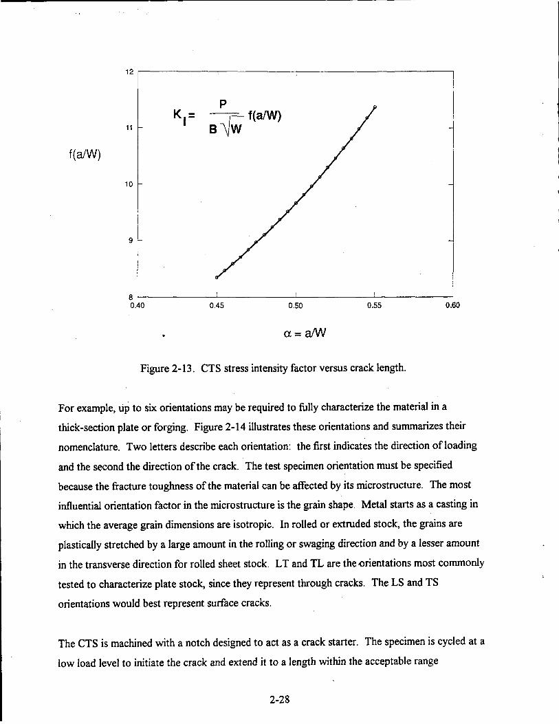
12

11

10

9

I

J 8 ‘ I I I 0.40 0.45 0.50 0.55 0.60

Figure 2-13. CTS stress intensity factor versus crack length.

For example, up to six orientations may be required to fully characterize the material in a

thick-section plate or forging. Figure 2- 14 illustrates these orientations and summarizes their

nomenclature. Two letters describe each orientation: the first indicates the direction of loading

and the second the direction of the crack. The test specimen orientation must be specified

because the fiacture toughness of the material can be affected by its microstructure. The most

influential orientation factor in the microstructure is the grain shape. Metal starts as a casting in

which the average grain dimensions are isotropic. In rolled or extruded stock, the grains are

plastically stretched by a large amount in the rolling or swaging direction and by a lesser amount

in the transverse direction for rolled sheet stock. LT and TL are the orientations most commonly

tested to characterize plate stock, since they represent through cracks. The LS and TS

orientations would best represent surface cracks.

The CTS is machined with a notch designed to act as a crack starter. The specimen is cycled at a

low load level to initiate the crack and extend it to a length within the acceptable range

2-28

Figure 2-14. CTS orientation.

Reprinted from Damage Tolerant Design Handbook, 1975, Fig. 2.0-la, by permission of Battelle, Columbus, Ohio.]

0.45 5 a/W I 0.55. (The crack is monitored by means of travelling microscopes, which are focused on the area ahead'of the notch on the front and back faces.) The test is then performed

by slowly increasing the applied load until the specimen fractures.

After testing, the crack length at which the fracture initiated is measured at three locations. The

crack length "a" is defined as the average of the three measurements, and the test is not accepted

if the difference between any two measurements is more than 10 percent of the average. The

criterion is designed to avoid errors due to specimen misalignment in the testing machine and/or

excessive influence of near-surface (plane stress) conditions. (Additional criteria which depend on

the notch machining details are given in ASTM Specification E-399.)

Close attention is also paid to the plot of applied load versus displacement of the testing machine

grips. A candidate load Po for use in the stress intensity factor formula is defined based on the

type of load-displacement plot obtained (see Figure 2-1 5). In each case, the initial slope of the

plot (P/v), must first be measured, and a straight secant line is then constructed from the origin

with a slope of 0.95 (Plv),. The intersection of the secant line with the plot defines a load called

Ps The candidate load Pe is then taken to be equal to Ps or the maximum load P-, depending on

I

2-29

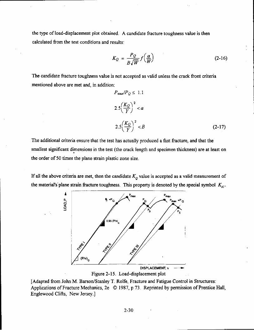
the type of load-displacement plot obtained. A candidate fracture toughness value is then

calculated from the test conditions and results:

(2- 16)

The candidate fracture toughness value is not accepted as valid unless the crack front criteria

mentioned above are met and, in addition: P,,/PQ 5 1 . 1

(2- 17)

The additional criteria ensure that the test has actually produced a fast fracture, and that the

smallest significant dimensions in the test (the crack length and specimen thickness) are at least on

the order of 50 times the plane strain plastic zone size. a

If all the above criteria are met, then the candidate Ke value is accepted as a valid measurement of

the material's'plane strain fracture toughness. This property is denoted by the special symbol KlC.

DISPLACEMENT, v - Figure 2-15. Load-displacement plot

[Adapted from John M. BarsodStanley T. Rolfe, Fracture and Fatigue Control in Structures: Applications of Fracture Mechanics, 2e 0 1987, p 73. Reprinted by permission of Prentice Hall, Englewood Clifts, New Jersey.]

2-30

Table 2-1 Properties of some common structural materials.

[fiom R. Pelloux, MIT, by permission] (see Figure 2-13 for orientations) Aluminum AUovs

2024 T3 : Flu

E%

LT* L LT L LT

2024 T851 LT Typical KIC [ksi(MPa 5)] 22(24.2)

2124 T85 1 LT Typical K~c[ksi(MPa,/iF)] 29(3 1.9)

a

2124 T85l Flu LT Fv LT

E% LT

Low Allov High Strenfzth Steel ( O&T)

US1 4340 UTS 200 ksi . . Yield 180 ksi

K*c 80 hi& UTS: Ultimate tensile strength

UTS 250 ksi Yield 240 ksi

Maraging Steel

K r 100 k s l h

66(455) ksi(MPa) 67 (461) ksi (MPa) 45 (3 10) ksi @Pa) 50 (345) ksi (MPa) 18

TL SL 20(22) 17( 18.7)

TL SL 24(26.4) 24(26.4)

66(455) ksi (MPa) 57(395) ksi (MPa) 8

250 ksi 300 ksi 240 ksi 290 hi 60 k s i 6 50 hi&

2-3 1

Table 2.1 Properties of some common structural materials. (continued)

Titanium

Ti 6Al-4V Equiaxed

Yield 130 ksi 40-6Oksifi 44-66 MFafi (910 MPa)

K I C Ti 6Al-6V-2 Sn

Yield

Stainless Steel

155 ksi 30-50 ks i f i 33 - 5 5 M P a f i (1085 MPa)

17-7 PH Yield 171 ksi 32 h i 5 35 MPafi (1180MPa)

k K I C

4286 Yield 1 12 ksi 152 k s i f i 167 M P a f i (769 MPa)

Alloy Medium Strength Steel . Yield 170 h i (1 175 m a )

0.35% C 0.65% Mn 0.35% Si 3% Ni 0.3% Mo 0.1% v 0.8% Cr

at

0°C K,c= llOksi& -100" c Krc=60 hi&

ref.): Application of Fracture Mechanics for Selection of Metallic Structural Materials, Eds. J. E. Campbell, W.W. Gerberich, and J.H. Underwood, ASM 1982.

Long Transverse

Since within certain limits, K,,is known for a given material, the engineer can use this value to

predict critical combinations of stress and crack length for many different configurations, once

stress intensity formulas such as those shown in Figure 2-7 are established.

2-32

It is worth repeating here that K, represents the stress intensity applied to a sharp crack in any

material, whereas K,, represents the ability of a specific material to resist fracture. In other

words, the applied loads and the stress analysis determine K,, while the material property

establishes that fiacture will occur when K, reaches K,, .

2.3.1 Thickness Effects

Why is so much attention paid to plane strain fracture toughness when so many structural

components are made of thin sheet stock? The plane strain condition separates the basic material

behavior from thickness effects. A change of thickness does not appreciably affect conventional

material properties. If the yield strength of a materid has been determined by testing a specimen

one inch thick, then we expect stock from 1/10 to 10 inches thick to have more or less the same

strength.

. Conversely, the strength of a cracked thin sheet is a strong hnction of thickness. Measurements

of candidate fracture toughness Ke typically follow a curve similar to the schematic example in

Figure 2-16. The results tend to approach the valid plane strain fracture toughness K,, in

specimens thicker than 1/2 inch. For thinner stock, however, KQ at first increases as the thickness

decreases and then declines after reaching a peak (generally at a thickness somewhat less than 1/8

CCP CTS NPICAL TEST SPECIMEN CONFIGURATION

- . -

I

1

I I I I F THICKNESS, B or t (in)

118 114 1 12 1

Figure 2- 16. Thickness effect on fiacture strength.

2-3 3

inch).] The peak KQ value can exceed five times K,c for some materials. Hence, the appropriate

KQ should be used in damage tolerance analysis. Note that Kc is used to denote a KQvalue

corresponding to plane stress conditions.

The thickness effect can be explained in terms of Griffith's energy balance idea, taking into

account the influence of plastic zone size. Figure 2-17(a) shows how the plastic zone varies through the thickness of a plate, along the crack front. Since or must be zero at the stress-free faces, the surface condition is plane stress, and the plastic zone is large. Well inside the specimen,

the surrounding elastic material restrains deformation in the z-direction. If the specimen is thick enough, the interior deformation is almost totally restrained ( E~ = 0), the condition is plane strain, and the plastic zone is small. Going inward from the surface, the plastic zone undergoes a

transition from larger to smaller size. The rate at which this transition progresses is approximately

independent of the total thickness.

Figure 2-17(b) illustrates end views of the plastic zones in plates of decreasing thickness. It is

evident that, as the thickness decreases, the ratio of total plastic volume to total thickness

increases. It then follows that the energy absorption rate per unit thickness must increase.

Conversely, the elastic stresses which provide the strain energy storehouse are uniform through

the thickness in most of the plate volume. Thus, the strain energy release rate is approximately

independent of thickness. When these factors are accounted for in the energy balance, it follows

that the thinner the plate, the more applied stress is needed to extend a crack. In other words, the

fracture toughness increases.

The plane stress effect leaves behind physical evidence of its presence on the fracture surface.

Under plane stress conditions the fracture plane tends to be tilted at a 45" angle to the z-axis,

unlike the plane strain condition which produces a fracture plane parallel to the z-axis. The tilted

regions are referred to as shear lips (Figure 2-18). The fracture surface of a valid K,c test Will

Stock less than 114 inch thick is generally tested in the form of a center cracked panel (Figure 2-7(a)) rather than a CTS.

2-34

t Y I BACK FACE:

PLANE ST

FRONT FACE:

(a) Three-dimensional plastic zone shape.

(b) Plastic volume versus thickness.

Figure 2- 17. Plane stress-plane strain transition.

2-3 5

Figure 2- 18. Typical fiacture sufiaces.

have little or no evidence of shear lips. Conversely, a ffacture surface with a high percentage of

shear lip indicates that plane stress conditions dominated the fiacture.

The foregoing analysis does not explain why Ke eventually declines as the thickness is decreased

still hrther. This phenomenon is a result of an increase in the strain energy release rate which

overpowers- the energy absorption rate increase associated with plane stress conditions. A

complete stress analysis of the region around the crack (not just the crack tip locality) shows that the stress ox is compressive in the areas above and below the crack (Figure 2-19).

A well-known property of thin plates loaded in compression is that they will buckle at some

critical stress proportional to the square of the ratio of thickness to unsupported span. (The

constant of proportionality depends on the manner in which the edges of the plate are supported.)

Evidently, the areas above and below the crack should behave in the same way, with a buckling

stress proportional to (th)’ . For a given crack length, it then follows that there will be some

2-3 6

thickness t,, for which the compressive'stress ox induced by the crack is just enough to cause local buckling when the applied stress is high enough to extend the crack. For t < t , , buckling

occurs and releases additional strain energy to drive the crack. The thinner the plate or the longer

the initial crack, the more strain energy is released, and this is why Ke declines. '

t Sit1 i f 1 1 SStS

Figure 2-19. Lateral compression above and below the crack.

Lateral bucklipg deflects the areas above and below the crack out of the xy plane, as shown in

Figure 2-20. This has the additional effect of applying a small amount of Mode III loading to the

crack tips, and fractures of this type are usually described as tearing. The lateral buckling

phenomenon can be easily observed if load is applied slowly in one of the aluminum foil

experiments with a long initial crack.

2.3.2 Temperature Effects

The fiacture toughness of a metal also depends on its temperature when tested. As its

temperature decreases, a metal becomes less able to accommodate the intense crack-tip stresses

by yielding, and the energy absorption rate y p decreases. As a result, KrC is found to decrease

2-37

with temperature, general!

Figure 2-20. Lateral buckling and tearing.

following an S-shaped curve like the schematics in Figure 2-2 1. This

phenomenon is sometimes referred to as a ductile/brittle transition.

Aluminum alloys are relatively insensitive to temperature over the range corresponding to aircraft

service conditions, but must be tested at low temperatures to obtain the correct K,,vdue for

applications such as pressure tanks designed to hold cryogenic liquids (LOX, LH, etc.).

Conversely, many steel alloys exhibit a sharp transition in the service temperature range, and the

complete transition curve is required to assess the structural strength at the lowest anticipated

service temperature.

2.4 FAILURE IN THE PRESENCE OF LARGE-SCALE YIELDING

Other means of strength assessment are required for structures which do not meet the small-scale

yielding condition. A variety of different methods and strength parameters have been developed

2-3 8

,

' l C i STEEL ALLOYS

ALUMINUM ALLOYS

. _ _ _ _ . . . . . - 4 _ _ _ _ - . . . . ...

I I A I I I I I *

-460 -423 -362 -70 0 5 0 150 STRATOSPHERE mcnm LH LOX

TEMPERATURE ( O F ) ZERO zMffi BMuNG POINT

Figuke 2-21. Fracture toughness versus temperature.

to deal with such situations. The R-curve method (Section 2.4.1) and the net section failure

criterion (Section 2.4.2) are widely used in the aeronautical industry. Both approaches have

prominent roles in airframe damage tolerance evaluation. Four other approaches, subjects of

theoretical and experimental research for many years, have not yet attracted industry attention but

might be used in the hture. The crack opening displacement and "J-integral" approaches

(Sections 2.4.3-and 2.4.4) are concepts for alternative strength properties used in place of fracture

toughness. The strain energy density criterion (Section 2.4.6) and the plasticcollapse model

(Section 2.4.7) are methods for dealing with mixed-mode loading and three-dimensional cracks.

2.4.1 Resistance Curves

The resistance curve or "R-curve" method was developed to provide reliable estimates for the

damage tolerance of plain or stiffened thin-skinned panels [2-13 to 2-17]. Early attempts to use

the apparent fracture toughness Kc (Section 2.3.1) as a fracture stability limit analogous to K,, gave inconsistent results.

2-39

The key to understanding thin-sheet fracture was discovered when researchers began to pay close

attention to the behavior of long initial cracks in large sheets as the applied stress was increased

toward the critical value. Based on the hndamental energy balance concept (Section 2. l), one

would not expect the crack to extend at all until the stress reached the critical value. Thick-section

specimens tended to behave as expected, although a small amount of crack extension just before

fracture was sometimes reported for intermediate thicknesses.' Conversely, measurements made

on thin sheets showed that a considerable amount of stable crack extension would occur at

stresses well below the critical value. Figure 2-22 compares the different types of behavior in

terms of applied stress intensity factor.

f- STABLE CRACK EXTENSION

STRESS 1

INTERMEDIATE I / \

v /

* . K

THICK 4 "POP-IN" (STABLE CRACK EXTENSION)

CRACK EXTENSION, Aa

Figure 2-22. Load versus crack extension for different thicknesses.

llus phenomenon is called "pop-in.'' 2

2-40

The concept of the R-curve method is that stable crack extension is a material property which can

be described as a relation between a stress intensity factor KR (obtained from a test) and crack

extension Au, independent of the initial crack length u,. The actual test is performed by placing a cracked specimen in a testing machine, increasing the applied load incrementally and allowing

sufficient time between steps for the crack to stabilize before measuring the new load and crack

length. R-curve tests are usually performed on large center-cracked panel specimens.

Consider the case shown in Figure 2-23 for a thin sheet of width Wcontaining an initial crack of

length 2u. As the applied stress is increased in steps to a1,02,03, etc., crack lengths 2u,, 2a2,

2a3, etc. are measured. The crack extension at each step Au is defined as the current value of a - a,, and KR is based on the formula for stress intensity factor for the center-cracked panel at the

current value of stress and crack length. Kcis taken as the value of K' at the onset of unstable

fracture. . This definition sometimes leads to the reporting of the R-curve asymptote as a "critical K" or K, value. However, K,as defined above is not strictly a material property, but also depends on the

initial crack length. This is simply a consequence of the fact that the strain energy release rate

depends upon total crack length, rather than crack extension.

A convenient way to visualize this fact is to overlay the R-curve on a plot of KI versus half crack

length for a fixed value of stress. Since the abscissa of the plot is hacrack length, rather than

crack extension, the base of the R-curve must be aligned with the initial half crack length a,.

Figure 2-24 illustrates KI plots for two stress levels: 01 and a?> 01. The Same R-curve has been overlaid at two positions: a,, and urn < a,,, such that each curve is just tangent to the

corresponding KI plot. Both cases represent fracture onset, i.e., the energy release rate always

equals or exceeds the energy absorption rate represented by the R-curve. However, note that the

K, values for the two cases are different. As indicated by the shaded areas, the elastic energy is at

first released at a slow pace controlled by the rate at which the applied stress is increased. At the

point of tangency, however, the structure becomes able to release energy faster than the extending

crack can absorb it, and fracture occurs.

.

2-41

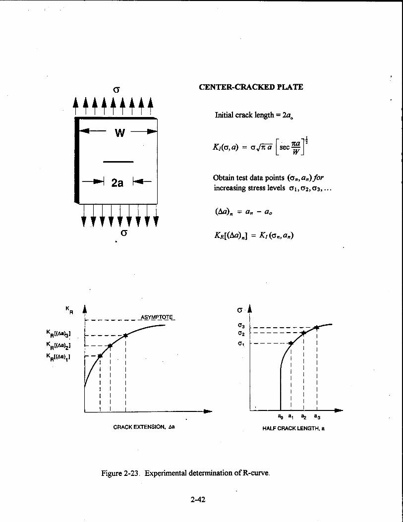
f S f f f f f f f

(T .

I w

CRACK EXTENSION, Aa

CENTER-CRACKED PLATE

Initial crack length = 2u,,

Obtain test data points (on, an) for increasing stress levels Q 1 , 0 2 , 0 3 , . . .

HALF CRACK LENGTH, a

Figure 2-23. Experimental determination of R-curve.

2-42

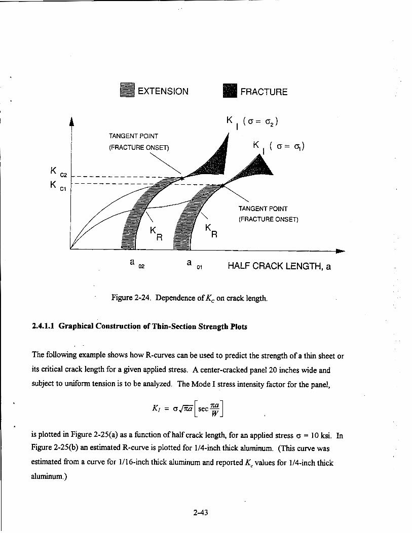
c2

c1

EXTENSION

TANGENT POINT

(FRACTURE ONSET)

FRACTURE

K , b= 0,) A

\ TANGENT POINT (FRACTURE ONSET)

a 02 a 01 HALF CRACK LENGTH, a

. Figure 2-24. Dependence of Kc on crack length.

2.4.1.1 Graphical Construction of Thin-Section Strength Plots

The following example shows how R-curves can be used to predict the strength of a thin sheet or

its critical crack length for a given applied stress. A center-cracked panel 20 inches wide and

subject to uniform tension is to be analyzed. The Mode I stress intensity factor for the panel,

KI = o J E i [ s e c ~ ]

' is plotted in Figure 2-25(a) as a hnction of half crack length, for an applied stress CJ = 10 ksi. In Figure 2-25@) an estimated R-curve is plotted for 1/4-inch thick aluminum. (This curve was

estimated fiom a curve for 1/16-inch thick aluminum and reported K, values for 1/4-inch thick

aluminum.)

2-43

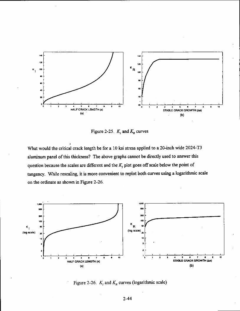
I K

0 1 2 3 4 5 E 7 8 0 IO

HALF CRACK LENGTH (a) (a)

Figure 2-25. Kl

What would the critical crack length be for a 10 ks

aluminum panel of this thickness’? The above grap

question because the scales are different and the K

tangency. While rescaling, it is more convenient ti on the ordinate as shown in Figure 2-26.

K I (log =aW

I .m,

500

2a

10

5

0 1 2 3 4 5 e 7 8 e 10

HALF CRACK LENGTH (a) (a)

140 -

R K

20 1 I I I I , I 1 I

0 1 2 3 4 5 8 7 a e 10

STABLE CRACK GROWTH (M)

(b)

nd KR curves

stress applied to a 20-inch wide 2024-T3

s cannot be directly used to answer this

plot goes off scale below the point of

replot both curves using a logarithmic scale

(log scale)

. Figure 2-26. K, and KR curves (logarithmic scale)

2-44

I -

O 1 2 ¶ 4 S 6 7 6 O 10 STABLE CRACK GROWTH (aa)

(b)

The R-curve can now be overlaid and aligned properly on the K, plot over the entire range of half

crack length. In figure 2-27, the R-curve has been overlaid to find the tangent point, which

corresponds to K, = 105 ksi fi. The base of the R-curve is located at a = 7.6 inches. Thus, the critical crack length (2a) is 15.2 inches.

1 I I I I I 1 - I I 1 I 1 I I I I I I 1 I

Figure 2-27. Overlay of KI and KR curves to determine critical crack length

Figures 2-28 and 2-29 contain enlarged copies of the logarithmic plots: The reader will find it

usefkl to make a transparency of the enlarged R-curve and repeat the above overlay procedure.

The enlarged Kl plot and R-curve overlay should also be used to follow through the rest of the

example.

2-45

100

KR

10

0 . 0 1.0 2 . 0 1.0 4.0 5 . 0 6 . 0 7 . 0 11.0 0.0 10.0

STABLE CRACK GROWTH (DELTA a1

Figure 2-28. R-Curve for 2024-T3

2-46

K APPLIED

0 . 0 1.0 2 . 0 3 . 0 4.0 5 . 0 6 . 0 7 . 0 11.0 B . 0 10.0

HALF CRACK LENGTH (a)

Figure 2-29. K applied versus crack length

2-47

One obvious question to ask is what one would estimate for the critical crack length if only the

"critical I?' value (132 hi &) had been reported and were treated as if it were like a &,value. If the overlay is flipped over (left to right reversal), the left side can be used as a "no-extension R-curve": vertical step at the left edge to K = 132 hi f i with a sharp comer. Overlaying this "R-curve" to find the tangent point puts the base at a = 9 inches. Thus, the improper use of a

reported Kc in this case would lead to an unconservative prediction of 18 inches for the critical

crack length (Figure 2-3 0).

0 1 2 3 4 5 6 7 8 HALF CRACK LENGTH (a)

I I j 1.000

I I I I I I I - 9 10

10 B

K R r. 8 7 6 5 . 4 3 2 1 0 '

STABLE CRACK GROWTH (h)

. . Figure 2-30. Use of critical K to determine critical crack length

The same two logarithmic plots can also be used to estimate the critical stress and crack length for

other values of applied stress. The R-curve is simply aligned to find the tangent point for a

specified half crack length. K, is then read directly from the R-curve overlay scale. The critical

stress oc can also be found by starting at 10 (the reference stress) on the scale K,and reading across to the R-curve scale.

For example, what is the critical stress for a crack length 2u = 8 inches? Figure 2-3 1 shows the

correct overlay position and the answers.

2-48

= 126 k s i f i

1,000~

1,000 500 : I

I 200

100 I 50

20 (T =10ksi 10

5

(be

ref

a = 4" 2 5 I I I I I I I I I

0 1 2 3 2 5 6 7 8 9 1 0 RACK LGNGTI-J (a) I I I I I I I

0 1 2 3 4 5 6 7 8 9 10 STABLE CRACK GROWTH ( Aa)

Figure 2-3 1 . Critical stress determinations with K, and KR curves.

The above procedure, originally invented by Creager [2-181, allows one to rapidly construct plots

of K, and a', versus crack length. These plots are shown in Figure 2-32 for the 20-inch wide aluminum panel example.

The R-curve approach is useful and practical for correlating the fracture resistance of typical

aircraft panel-and-stringer construction, but limitations still exist. The most useful application is

to damage tolerance assessment of situations involving an isolated long crack, since R-curves are

typically derived from tests of single long cracks in wide panels. However, KR depends on section

thickness as well as alloy material, and only a few curves for a few skin thicknesses have been

published in the open literature. Several examples from references [2-161 and [2-191 have been

I

' reproduced in Appendix B.

2-49

5 0 -

4 0 -

3 0 -

2 0 -

10 -

U C

(ksi)

1 o ~ " ' l ' l ' l ' l " ' l . ' . l .

- ~ " " " " ' ~ ~ ' ~ ~ ~ ' ~ '

0 1 2 3 4 6 7 8 8 1 0 5 0 1 2 3 4 5 6 7 8 0 1 0 HALF CRACK LENGTH a ( In) HALF CRACK LENGTH a (In)

b

Figure 2-32. Kc and CT vs. a for a 20-inch aluminum panel.

Another important limitation is that the R-curve does not strictly depend on crack extension

alone. What really counts is the volume of new material that undergoes plastic deformation when

the crack extends. Figure 2-33 illustrates three different examples of what can happen. In

example (a), a crack has extended from an initial length 2ao, much larger than the plastic zone size

to a length &-I, much smaller than the panel width. The contoured areas depict the new plastic

volumes, which are independent of each other and the panel edges.

Example (b) shows what happens when the initial crack length is of the same order as the plastic

zone size. Example (c) shows what happens when the initial crack is long enough to place the

crack tips near the panel edges. In example (b), the two crack-tip stress concentrations reinforce

each other, while in example (c) the nearby free edge reduces the panel's ability to constrain the

deformation. In both cases, the result is a larger plastic volume for the same crack extension as in example (a), i.e., an R-curve derived from a test of a medium-length crack should not be expected

to characterize the strength of similar bodies with very long or very short cracks.

2-50

. -

(a) Isolated medium or long crack.

(b) Short crack. I I

FREE EDGE

I - (c) One crack tip near edge of a panel.

Figure 2-33. Effect of surroundings on energy absorption rate.

2-5 1

2.4.2 The Net Section Failure Criterion

The net section failure criterion has its roots in the traditional static strength design practices used

by the aeronautical industry almost ever since airframes have been made from metal. Joints made

with bolts or rivets have always played a prominent role in metal airflames The skins or webs in

these joints were subject to stress concentration around each fastener hole, but early designers of

metal airframes had neither the modem numerical stress analysis methods nor the computers

which the methods require. Therefore, approximate methods of analysis which could be carried

out by hand calculation were highly valued.

The net section failure criterion was one quch method. The criterion was based on observations

that ductile metals subjected to concentrated stress tend to reduce the stress when they yield.

There was ample field experience to support these observations. For example, if one fastener in a

joint happened to have an excessive bearing load because parts had been misaligned when the

holes were drilled, the parts would yield under load and deform until the fastener bearing forces

were equalized.

From the foregoing observations, it was a short step to the hypothesis that the elastic stress

concentrations around all of the fastener holes in a joint would be progressively smoothed out, as

the applied load increased, until the tension across the minimum ("net") section between the holes

was distributed uniformly just as the stress level reached the material's ultimate strength. Thus,

the critical load capacity of the joint could be estimated as the product of the net section area and

the ultimate strength.

Figure 2-34 shows how the net section failure criterion is applied to a tensile coupon of width W containing an open hole of diameter D. At low stress, the coupon r'emains elastic, and a stress

concentration factor of 3 is realized. As the applied stress is increased, yielding progresses from the edge of the hole until the net section (W - 0) t is stressed to the ultimate tensile strength csult. The critical load is then estimated as P = Q,, ( W - D) f.

2-52

t ""I w 3

ELASTIC YIELDED

m ULTIMATE

Figure 2-34. Net section failure criterion.

In its simplest form, the net section failure criterion tends to overestimate the critical load because

there are other components of stress besides the principal tension in the yielded region.

Consequently, the criterion is modified for practical application by substituting a so-called "flow

stress'' of for the ultimate strength, based on correlation with strength tests of coupons like the one shown in Figure 2-34. Extensive tests on aluminum coupons suggest that the flow stress for

alloys used in &rframes ranges from five percent above the yield strength to five percent below

the ultimate strength.

It is a natural step to apply the net section failure criterion to thin sheets containing cracks, even

though the criterion does not account for stable crack extension. In this case, the critical crack

length plays the role which was played by the fastener hole diameter. Thus, for example, the net

section in a thin sheet of width W containing a center crack of length 2a is ( W - 2a)t, and the

critical applied stress (load divided by nominal area) is:

.

W - 2u W *f oc = (2- 1 8)

2-53

2.4.2.1 Failure Mode Determination and the Feddersen Diagram

When should the net section failure criterion be used in place of the R-curve method to estimate

the strength of a cracked thin sheet? The answer is obtained by comparing the strength plots for a

specific situation.

In the example R-curve analysis presented in Section 2.4.1, an R-curve strength plot was

constructed for a 1/4-inch thick 2024-T3 sheet 20 inches wide. A reasonable choice for the flow

stress of 2024-T3 aluminum might be of = 48 ksi. A net section strength plot based on this flow stress is shown in Figure 2-35 together with the R-curve strength plot &om the preceding section.

It is evident from the comparison that the R-curve strength estimate is unconsewative for crack

lengths shorter than 2a = 4 inches and longer than 15 inches in this case.

oc (ksi)

CENTER-CRACKED PANEL w = 2 ~ 9 , t = iw 2024-T3

\ NETSECTION 7

I I I 1

HALF CRACK LENGTH a (in) 4 6 88 10 0 2

Figure 2-35. Net section and R-curve strength curves.

2-54

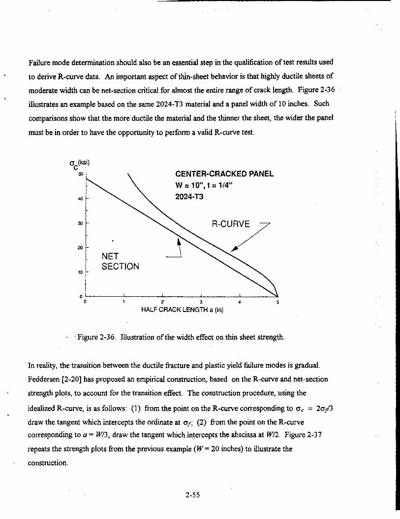
Failure mode determination should also be an essential step in the qualification of test results used

to derive R-curve data. An important aspect of thin-sheet behavior is that highly ductile sheets of moderate width can be net-section critical for almost the entire range of crack length. Figure 2-36

illustrates an example based on the same 2024-T3 material and a panel width of 10 inches. Such

comparisons show that the more ductile the material and the thinner the sheet, the wider the panel

must be in order to have the opportunity to perform a valid R-curve test.

CENTER-CRACKED PANEL W = 1 O", t = 114"

30-

2 0 -

SECTION 10 -

1 2 3 4 5 0

HALF CRACK LENGTH a (in)

. - Figure 2-36. Illustration of the width effect on thin sheet strength.

In reality, the transition between the ductile fiacture and plastic yield failure modes is gradual.

Feddersen [2-201 has proposed an empirical construction, based on the R-curve and net-section

strength plots, to account for the transition effect. The construction procedure, using the

idealized R-curve, is as follows: (1) from the point on the R-curve coriesponding to oc = 20j3

draw the tangent which intercepts the ordinate at of; (2) fkom the point on the R-curve corresponding to a = W/3, draw the tangent which intercepts the abscissa at W/2. Figure 2-37

repeats the strength plots fiom the previous example (W= 20 inches) to illustrate the

-

' construction.

2-55

The strength envelope consisting of the two tangent lines and the included segment of the R-curve

is called a Feddersen diagram. Before an R-curve derived from a panel test is accepted, it should

be verified that the initial crack length lies in the included R-curve segment on the Feddersen

diagram.

OC

(ksi) CENTER-CRACKED PANEL

O f =48 w = 20", t = 1/4"

30 - =28 f 2 0

3 20-

10 -

a 10

I I

I I

2 4 6 1 8

HALF CRACK LENGTH a (in) 0

I I I

Wl3 Wl2

Figure 2-37. Construction of Feddersen diagram.

2.4.3 Crack Opening Displacement

Determination of the onset of unstable crack propagation by means of measurement of crack

opening displacement is another approach to the problem of fracture with large-scale yielding.

Crack opening displacement (COD)3 can be used as a fracture toughness parameter in a similar

manner to Krc, i.e., at a critical value of COD a crack will propagate unstably. The advantage of the COD approach is that COD values can be measured throughout the entire plane strain,

elastic-plastic, and hlly plastic behavior regions.

The common definition of COD is the displacement at the crack mouth, as measured by means of a clip gauge, and sometimes called CMOD. However, some models are based on the so-called crack tip opening displacement (CTOD), which is actually an extrapolation.

2-56

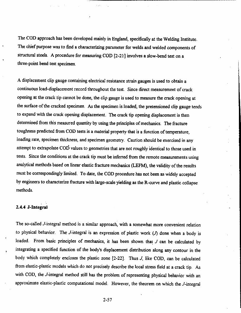
The COD approach has been developed mainly in England, specifically at the Welding Institute.

The chief purpose was to find a characterizing parameter for welds and welded components of

structural steels. A procedure for measuring COD [2-211 involves a slow-bend test on a

three-point bend test specimen.

A displacement clip gauge containing electrical resistance strain gauges is used to obtain a

continuous load-displacement record throughout the test. Since direct measurement of crack

opening at the crack tip cannot be done, the clip gauge is used to measure the crack opening at

the surface of the cracked specimen. As the specimen is loaded, the pretensioned clip gauge tends

to expand with the crack opening displacement. The crack tip opening displacement is then

determined fiom this measured quantity by using the principles of mechanics. The fracture

toughness predicted fiom COD tests is a material property that is a finction of temperature,

loading rate, specimen thickness, and specimen geometry. Caution should be exercised in any

attempt to extrapolate COD values to geometries that are not roughly identical to those used in tests. Since the conditions at the crack tip must be inferred fiom the remote measurements using

analytical methods based on linear elastic fracture mechanics (LEFM), the validity of the results

must be correspondingly limited. To date, the COD procedure has not been as widely accepted

by engineers to characterize fiacture with large-scale yielding as the R-curve and plastic collapse

methods.

2.4.4 J-Intebal

The so-called J-integral method is a similar approach, with a somewhat more convenient relation

to physical behavior. The J-integral is an expression of plastic work Q done when a body is 1

loaded. From basic principles of mechanics, it has been shown that J can be calculated by

integrating a specified fbnction of the body's displacement distribution along any contour in the

body which completely encloses the plastic zone [2-221. Thus J , like COD, can be calculated fiom elastic-plastic models which do not precisely describe the local stress field at a crack tip. As

with COD, the J-integral method still has the problem of representing physical behavior with an

approximate elastic-plastic computational model. However, the theorem on which the J-integral

t

is based extends to the boundaries of the body, and it has been shown that simple measurements

of plastic work (e.g., the product of applied load and testing machine crosshead travel) are

equivalent to J . The J-integral method is occasionally applied in the course of ad hoc assessments

of the integrity of ductile structures but has not been reduced to routine engineering practice.

2.4.5 Practical Developments

As the concept of fracture mechanics began to be widely applied to airframe damage tolerance

evaluation in the early 1970s, the evaluators had to extrapolate the stress intensity factor formulas

in ways not envisioned by the founders of the theory. The problem was that cracks in real

structures often displayed a three-dimensional character, whereas GrifEth’s energy analysis, Ixwin’s

stress solution, and most of the related developments have a fbndamentally two-dimensional

nature. . The two-dimensional character is built into the theories by the basic assumptions that the cracked

structure has a two-dimensional geometry and that the crack extends along its own line. Thus,

one must deal .with through-cracks having flat &aces in areas of structure where (at least near

the crack) the thickness is constant and any details such as fastener holes are through-drilled with

no taper or co~ntersink.~ Even the simplest of these situations has at least one three-dimensional

aspect: the transition from plane strain to plane stress conditions at the lateral faces of the

structure. Fortunately, the theories were found to work well enough in practice despite this

inconsistency when empirical modifications were made to account for thickness effects (e.g., the

R-curve method).

Conversely, some of the cracking encountered in real structures introduced other three-

dimensional factors that fbndamentally contradicted the theoretical assumptions.

One other valid case is a circular (“penny-shaped”) internal crack in a body large enough so that free-swface 4

effects can be neglected. The geometry is still two-dimensional in this case because of axial symmetry (see Section 2.5).

2-58

Figure 2-38 illustrates some typical examples, and the following paragraphs indicate the ad hoc

nature of the procedures that damage tolerance evaluators had to adopt.

*

Example (a) is a common type of fatigue crack which remains flat-surfaced but changes the shape

of its crack front as it extends. This is not normally a problem for strength analysis because such

cracks have generally become through-cracks well before reaching critical size. However, the

change of shape does affect the stress intensity factor which must be used to estimate the slow I

I

Example (b) shows an internal surface flaw in the wall of a high-pressure gas cylinder. The

problem in this case involves more than the estimation of critical crack size. A much more serious

question is how long the flaw can be in relation to its depth without risk of bursting the cylinder.

Whatever basic method of strength determination is used (Klc, R-curve, etc.), the analyst must

still make a judgment based on a comparison of critical stresses for the assumed flaw and an

equivalent through-crack of the same length.

Example (c) ilhstrates a typical through-crack which may be found at the comers of ibselage

fiame cutouts. The crack may not be aligned across the frame when it reaches critical size, and so may change direction when it fractures. In such cases, analysts often resort to straight crack

models which reproduce some key characteristic of the actual crack. Two possible choices are

shown: (1) fiacture assumed along the original crack lime; or (2) a crack across the tension and

of a length such that the fiame is cut to the same height as the actual crack.

While the ad hoc procedures have proved to be useful for making estimates of damage tolerance,

they are not well-founded and require frequent calibration by comparing estimates with test

results. This limitation is one reason why researchers continue to develop theories of fiacture

strength such as those summarized in the next two sections.

2-59

CRACK ORIGIN R I

u SUCCESSIVE P O S I T I O N d d

OF CRACK FROHT DURING SLOW GROWTH IN FATIGUE

SECTION A 4

N L / / BULBANGLE STRINGER

ArrACHED TO SKIN BY RIVETS

(a) Comer crack at a fastener hole.

VERSUS

MODEL

\

INTERNAL SURFACE CRACK SUBJECTED TO HOOP TENSION

A PRESSURE

HIGH - PRESSURE SECTION A-A

AVIATION OXYGEN CYLINDER

(b) Axial crack in an oxygen cylinder.

4 4- 4 +

(c) Through-crack at a fbselage fiame comer detail.

Figure 2-3 8. Typical examples of three-dimensional aspects of cracks.

2-60

2.4.6 Strain Energy Density Criterion

The strain energy density criterion was developed by Sih in the 1970s [2-23,2-241 and was

originally applied to problems in linear elastic fiacture mechanics. Later, the criterion was found

to be applicable to ductile fiacture as well [2-25,2-26,2-271.

We saw earlier that strain energy density is proportional to the square of stress, and that the

stresses near a crack tip in an elastic body are proportional to l / f i , where r is the radial distance from the crack tip. Therefore, the strain energy density at any point near the crack tip

can be expressed as:

(2- 19) u = - S r

where S is called the strain energy density factor and, like the stress intensity factor, depends only

on the externally appliedloads, the crack length, and the geometry of the structure. Since the

material has been assumed to be elastic, the strain energy density factor can be expressed in terms

of the stress intensity factors for the different modes of fiacture:

- 1 a,, - - sin 8 (COS 8 - 1 + 2 v ) 8 w

(2-20)

(2-2 1)

where v is the Poisson's ratio and E

= 2(1 + v) is the shear modulus.

2-6 1

From these expressions, it is evident that the criterion can be applied to problems that include

mixed modes

We have also seen that the local stresses lose their l/J7 character in the plastic zone Conversely, as long as the strain energy density is properly calculated as the area under the

stress-strain curve, it can be shown that Uretains its I/r character even when plastic deformation

occurs Thus, it is possible to calculate the strain energy density fbctor S at any point in a body,

as long as numerical results are available from an elastic-plastic stress analysis

Sih's criterion is based on a fbndamental property of the strain energy density finction under

conditions of plane strain Sih found that, when the stresses at any point in a body are expressed

in terms of principal stresses o,, a,, and a3 = v(a, + a, ), the strain energy density U could be expressed as a sum of two terms:

. u=U'+u" (2-22)

U' = l+v [ 0 , + 0 , + v ( G , + 0 J 1 2 - - + v [ Old2 + v(a1 + 0 2 ) 2 1 3E E

-2v [a, + az+ v (a, + 03y U = 6 E

(2-23)

(2-24)

where U' contains all the energy associated with shear and U" contains all the energy associated

with volume expansion Sih suggested that the likelihood of crack extension should increase

when the ratio of expansion to shear energy increases When he used equations (2-23) and (2-24)

to calculate U"/U', he found that the ratio increases steadily as the values of 01 and 02 approach each other.

Applying this idea to the local stresses near a crack tip, Sih also showed that when the total strain

energy density U is a minimum, U" is much greater than U' [2-281. Thus, when the strain energy

density factor S is expressed in terms of the Irwin solution (see Section 2.2), the minimum defines

the angle 8 at which the crack should extend (Figure 2-39) The hypothesis is consistent with the

2-62

I

known behavior of cracks subjected to Mode I loading ( 0 = 0), but it also gives other crack extension angles for mixed-mode loading.

Figure 2-39. Strain energy density criterion.

The amount and character of the crack extension is governed by two parameters which can be

derived fiom conventiond material properties. The critical strain energy density Uc is equated to

the area under the elastic-plastic stress-strain curve obtained fiom a tension test (Figure 2-40).

This definition is based on the assumption that the tensile stress-strain curve is also the equivalent

plastic stress versus equivalent plastic strain curve (a hypothesis commonly adopted in

elastic-plastic stress analysis). One physical interpretation of Uc is that crack extension must somehow be associated with exhaustion of the ductility of the material around the crack tip.

STRESS 1 TEST

STRAIN

Figure 2-40. Definition of critical strain energy density.

2-63

The critical strain energy density factor S, is related to the plane strain fracture toughness via the

Irwin solution. Since is obtained from a test with pure Mode I loading, it follows from equation (2-20) that:

sc =a& (2-25)

A third parameter re is derived from the first two parameters:

- S C rc - - UC

(2-26)

Application of the strain energy density criterion to practical problems requires a numerical

elastic-plastic stress analysis from which the strain energy density factor can be calculated. In any

xy plane like the one shown in Figure 2-40 the criterion is applied by calculating the crack

extension r = S / u . The extension is considered to be stable as long as r < rc , and fiacture is

assumed to occur whpn r first reaches the critical value.

The strain energy density criterion is applied to three-dimensional cracks by repeating the above

analysis in several xy planes spaced through the thickness. Since the results of the three-

dimensional stress analysis may vary through the thickness, different crack extension values (r, 0) will generally be calculated for each plane, i.e., the criterion can be used to deal with cracks of

arbitrary shape.

2.4.7 Plastic Collapse Model

The plastic collapse model was originally developed by Erdogan [2-291 to estimate the strength of

high-pressure gas transmission pipelines with surface or internal wall cracks. Gas transmission

pipelines are made of highly ductile steels which can be either fracture critical or net section

critical depending on the crack dimensions, wall thickness, and pressure stress levels. The

situation is fUrther complicated by the fact that under typical operating pressures the wall area

around the crack tends to bulge outward and distort the local distribution of stress.

2-64

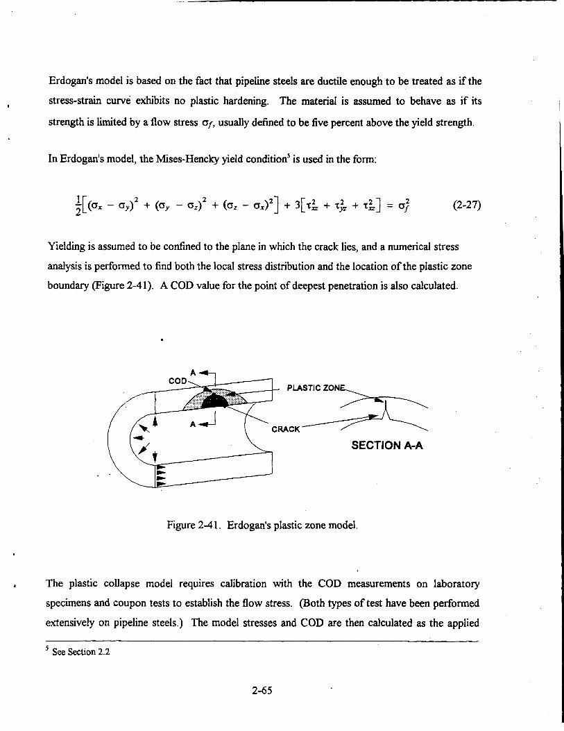
Erdogan's model is based on the fact that pipeline steels are ductile enough to be treated as if the

stress-strain curve exhibits no plastic hardening. The material is assumed to behave as if its

strength is limited by a flow stress of, usually defined to be five percent above the yield strength.

In Erdogan's model, the Mises-Henclq yield condition' is used in the form:

(2-27)

Yielding is assumed to be confined to the plane in which the crack lies, and a numerical stress

analysis is performed to find both the local stress distribution and the location of the plastic zone

boundary (Figure 2-41). A COD value for the point of deepest penetration is also calculated.

CRACK

SECTION A-A

Figure 2-4 1. Erdogan's plastic zone model.

I The plastic collapse model requires calibration with the COD measurements on laboratory

specimens and coupon tests to establish the flow stress. (Both types of test have been performed

extensively on pipeline steels.) The model stresses and COD are then calculated as the applied

See Section 2.2 5

2-65

load is increased in a series of small steps. No provision is made to account for stable crack

extension, but the critical load and failure mode are determined when one of the following two

conditions is first met: (1) the calculated COD reaches the critical value determined from

specimen tests; or (2) the plastic zone grows so rapidly that it would spread through the entire

section containing the crack plane ifthe load were increased again. These two conditions are

analogous to ductile fracture (with no R-curve effect) and net section fdure, respectively.

2.5 INTERNAL, SURFACE, AND CORNER CRACKS

The foregoing discussion has implicitly assumed a two-dimensional configuration of the cracked

body, e.g., a skin panel with a through-thickness crack. The stress fields associated with such

cracks are also two-dimensional for practical purposes (i.e., the stresses are uniform through the

thickness), except for panels subjected to out-of-plane bending loads. In the latter case, a

two-dimensional treatment by means of conventional plate and shell theories is also appropriate.6

However, many practical cracking situations have a three-dimensional character. Fatigue and/or

corrosion damage generally appears in the form of small surface or comer cracks. Although these

cracks are not likely to produce immediate fracture under service loads, it is important to

characterize their stress intensity factors for the purpose of estimating crack growth life (see

Chapter 3 ).

The basic solution for such situations is the Sneddon formula [2-301 for the stress intensity factor

of a circular ("penny") crack in an unbounded solid elastic medium:

KI = 20 E (2-28)

where a is a uniform tensile stress applied to the body and directed perpendicular to the plane of the crack, and a is the crack radius. Shah and Kobayashi have extended Sneddon's formula to

The bending stresses are assumed to be zero at the panel midplane (neutral plane for panel-stringer combinations) and to vary linearly through the thickness.

2-66

I

deal with elliptical cracks subjected to unifonn tension and/or bending, either in unbounded bodies

or located near a free surface [2-3 1,2-321. Approximate solutions have also been derived from

these results for the stress intensity factors associated with half-ellipse cracks extending inward

from a free surface and comer cracks extending inward from two free surfaces intersecting at

right angles, with either circular or elliptical arcs defining the crack front [2-331.

The approximate stress intensity factors for surface and corner cracks are routinely used in

damage tolerance assessments. These factors are expressed in the form: t

for the stress intensity at the deepest point of penetration7 through the thickness, where MK1, MKz and Q are factors depending on the crack shape (Figures 2 4 2 , 2 4 3 and 2-44).

For stress intensity factor solutions of various other crack configurations, see Appendix A and ref [ 2-3 41.

2.6 ENVIRONMENTAL EFFECTS

Fracture toughness is not directly affected by corrosive environments. However, some

high-strength materials may experience rapid crack propagation when subjected to static load

while immersed in a corrosive medium. This phenomenon, known as stress corrosion cracking, is

an extreme example of crack growth driven by chemical attack at the crack front. (”he static load

serves to hold the crack open, allowing circulation and m s i o n to continually replenish the

corrosive medium at the crack front.) For a given load, the crack grows at a constant rate with

respect to time. Material susceptibility is determined by means of a series of static tests at

decreasing loads, until a threshold for stress corrosion cracking is established. The corresponding

stress intensity factor KIxc is reported as the threshold property.’ For susceptible high-strength

materials, KIgc is much smaller than KIc. ~~

This is also the maximum stress intensity. The terminology was recently changed to “environmentally assisted cracking” with corresponding nomenclature

7

8

G A c *

2-67

b

A I J L

At point A: K,= 1.12M, OF b

for b/2a < 0.5, (Mkl = 1.12)

(a) Flaw shape parameter for surface flaws.

At point A: K, = 1.25 M, cs - E ' for b/2a < 0.5, (Mk, = 1.12 x 1.12 z 1.25)

(b) Flaw shape parameter for internal flaws.

Figure 2-42. Geometries of surface and comer cracks.

2-68

CT = gross stress o,, = yield strength

z

4

r) c

0.5 I I I I I I I I . 1 I

Figure 2-43. Stress intensity factors for surface and comer cracks.

Reprinted fiorn Damage Tolerant Desirn Handbook, 1975, Fig. 1 1 .1 .1 -1 , by permission of Battelle, Columbus, Ohio.]

2-69

I .7 I I I I I I I

a

1 6 -

Crack DepthICmck - 0 20 Length Rotlo - o 2s

2 I s -

L

U m LL

0

U m V * c p 1.3 - S

3

c 1 4 - c

c

c

E

g 1 2 -

- LL

0. al

I I -

I O

Crack Depth/ Specimen Thickness Rat10

Figure 2-44. Deep flaw magnification factor curves.

[Reprinted from Damape - Tolerant Design Handbook , 1975, Fig. 1 1.1.1-2, by pehssion of Battelle, Columbus, Ohio.]

2-70


2-1. Timoshenko, S.P. History of Strengzth ofMaterials, McGraw-Hill, 1953.

2-2. Inglis, C.E., "Stresses in a Plate Due to the Presence of Cracks and Sharp Corners," Transactions of the Institute of Naval Architects, Vol55,2 19-23 1, 19 13.

2-3. Gordon, J.E., Structures or Whv Things Don't Fall Down, Plenum Press, 1978.

2-4. m t h , A.A., "The Phenomenon of Rupture and Flow in Solids," Philos~~hical Transactions of the Roval Society of London, A221, 163-197, 1920.

2-5. Irwin, G.R., "Analysis of Stresses and Strains Near the End of a Crack Traversing a Plate," Trans. ASME. J. ADD]. Mech., Vol. E24, 1957, 361.

2-6. Tada, H., Paris P.C., and Irwin G.R., The Stress Analysis of Cracks Handbook, Del Research Corporation, Hellertown, PA, 1973.

2-7. Rooke, D.P., and Cartwright, D.J., Compendium of Stress Intensity Factors, H.M., Stationery Office, Lindon, 1975.

2-8. Sih, G.C., Handbook of Stress Intensity Factors, Lehigh University, Bethlehem, PA, 1973.

2-9. Murakami, Y. (ed.), Stress Intensity Factors Handbook, Pergamon Press, New York, 1987.

2- 10. Irwin, G.R., "Fracture Dynamics," Fracturing of Metals, American Society for Metals, 147-166, 1948.

2-1 1 . Orowan, E., "Fracture and Strength of Solids," Reports on Progress in Physics, XII, 185, 1948.

2-12. Standard Method of Test for Plane-Strain Fracture Touwess of Metallic Materials, ASTM E-399-83, American Society for Testing Materials, 1985.

2-13. Barsom, J.M., and Rolfe, S. T., Fracture and Fatigue Control in Structures, 2nd Edition, Prentice-Hall 1987.

2-14. Kanninen, M.F., and Popelar, C. H., Advanced Fracture Mechanics, Oxford University Press, New York 1985.

2-1 5. Broek, D., The Practical Use of Fracture Mechanics, Kluwer Academic Publishers, Dordrecht, Netherlands, 1988.

2-71

2-16. McCabe, D.E. (ed.), F), ASTM STP 527, American Society for Testing and Materials, Philadelphia, PA, 1973.

2-17. Standard Practice for R-Curve Determination, ASTM Standard E-561-81, Vol03.01, Metal-Mechanical Testing.

2-18. Creager, M., "A Note on the Use of a Simplified Technique for Failure Prediction Using Resistance Curves," Fracture Tourzhness Evaluation bv R-Curve Methods, ASTM STP 527, American Society for Testing and Materials, Philadelphia, PA, 1973.

2-19. Ratwani, M.M. and Wilhem, D.P. DeveloDment and Evaluation of Methods of Plane Strain Fracture Analvsis, Northrop Corporation, Aircraft Division, Los Angeles, CA, AFFDL-TR-73-42, Apd 1975.

2-20. Feddersen, C.E., Evaluation and Prediction of the Residual Strengh of Center-Cracked Panels. ASTM STP 486, American Society for Testing and Materials, Philadelphia, PA, 1970.

2-21. British Standard Institution BS5762, Methods for Crack OpeninP DisDlacement Testing, BSI (1979), London.

2-22. Rice, J.R., "A Path Independent Integral and the Approximate Analysis of Strain Concentration by Notches and Cracks, I' Journal of Applied Mechanics, 35,379-386, 1968.

2-23. Sih, G.C:, "Strain-Energy-Density Factor Applied to Mixed Mode Crack Problems," International Journal of Fracture 10, 305-321, 1973.

2-24. Sih, G.C., "Some Basic Problems in Fracture Mechanics and New Concepts," Endneering Fracture Mechanics 5,365-377, 1974.

2-25. Sih, G.C., and Madenci, E., "Fracture Initiation Under G~QSS Yielding, Strain Energy Density Criterion" Enrrineering Fracture Mechanics 18,667-677,1983.

2-26. Sih, G.C. and Chen, C., "Non-self-similar Crack Growth in Elastic-Plastic Finite Thickness Plate," Theoretical and Applied Fracture Mechanics 3, 125-139, 1985.

2-27. Sih, G.C., "Fracture Mechanics of Engineering Structural Components," in Fracture Mechanics Methodolow: DamaFe Evaluation of Structural ComDonents Intemity (Sih, G.C. and de 0. Faria, L. ed.), Martinus Nijhoff, Netherlands, 1984.

2-28. Sih, G.C. and MacDonald, B., "Fracture Mechanics Applied to Engineering Problems-Strain Energy Density Fracture Criterion," Engineering Fracture Mechanics 6, 361-386, 1974.

2-72

2-29. Erdogan, F., Theoretical and Experimental Studv of Fracture in Pipelines Containing Circumferential Flaws, Lehigh University, Bethlehem, PA, DOT-RSPA-DMA-50/83/3 (1982).

2-30. Sneddon, I.N., "The Distribution of Stress in the Neighbourhood of a Crack in an Elastic Solid," Proceedings of the Roval Society 4 187-229 (1946).

2-3 1. Shah, R.C. and Kobayashi, A.S., "Stress Intensity Factor for an Elliptical Crack Under Arbitrary Normal Loading," Engineering Fracture Mechanics 3,71-96 (1971).

2-32. Shah, R.C. and Kobayashi, A.S., 'Stress Intensity Factor for an Elliptical Crack Approaching the Surface of a Semi-Infinite Solid," International Journal of Fracture 9, 133-146 (1973).

2-33. Campbell, J.E., Damage Tolerant Desirn Handbook, Metals and Ceramics Information Center, Battelle Columbus Laboratories, 505 King Avenue, Columbus, OH 43201, MCIC-HB-0 1 , 1 975.

2-34. Gallagher, J.P., Giessler, F.J., and Berens, A.P., USAF Damage Tolerant Design Handbook: Guidelines for the Analvsis and Desi? of Damage Tolerant Aircraft Structures, Flight Dynamics Laboratory, Air Force Wright Aeronautical Laboratories, Wright-Patterson Air Force Base, OH 45433, MAL-TR-82-3073, May 1984.

2-73

a

FATIGUE CRACK PROPAGATION

. -

CHAPTER 3:

3. FATIGUE CRACK PROPAGATION

Fatigue crack propagation was not treated as a subject separate fiom fatigue failure until the

mid-1960s. Before then engineers were accustomed to dealing with metal fatigue based on

time-to-failure data (see Chapter 1). They understood that a crack had to form and propagate to

fail a test specimen, but they recognized that crack formation consumed most of the time, and

they saw no need to consider the relatively short propagation phase as a sigdicant phenomenon

in its own right.' After all, structures were not intentionally built with cracks in them, and fatigue

life (time to crack occurrence) was therefore the main concern for the designer. Not until 1970

did engineers begin to realize the importance of crack propagation as a distinct aspect of

structural damage tolerance.2 Laboratory and theoretical studies of crack propagation paved the

way for that advance.

3.1 ENERGY-BASED THEORY OF CRACK PROPAGATION

In the mid-l960s, research scientists working in the field of fiacture mechanics began to consider

the effects of repeated subcritical loads on cracks fiom an energy viewpoint.

Grif€ith's energy balance concept of fiacture did not include stable crack extension, but the

contradiction could be addressed by arguments based on the "pop-in" phenomenon. Recall that a

small but measurable stable crack extension ("pop-in") is observed in some fracture toughness

tests as the critical load is approached. One could then postulate that crack extension would be

proportional to the stress intensity factor range at lower loads but too small to measure (Figure

3-1).3

Crack formation typically consumes 95 percent of the measured Me of a rotating bending fatigue test specimen. The percentages for other common types of fatigue test specimens are comparable.

The effect of crack propagation was dramatically demonstrated by the crash of an F-1 1 1 at Nellis Air Force Base, Nevada in 1969. The crash was caused by the catastrophic failure of the wing cany-through box lower skin during a training mission. An extremely large forging flaw in the skin propagated to critical size in 105 flight hours. Based on the older fatigue analysis approach, the F-1 1 1 airframe was estimated to have a safe-life of 8,000 flight hours.

tolerance analyses, the simpler notation K is used to represent K,in this chapter.

1

2

Since Mode I loading is used in most laboratory fatigue crack growth tests and is assumed in most damage 3

3-1

I

ACTUAL EXENSION BELOW F- MEASURED "POP-IN

RESOLVING POWER /

OF MEASUREMENT

POSTULATED

BEHAVIOR

r

CRACK EXTENSION, Aa

Figure 3-1. Argument for relating fatigue crack growth rate to applied stress intensity factor.

Fatigue crack propagation was explained by hrther assuming that repeated cycles fiom zero load

to the same stress intensity factor K would cause the same amount of crack extension per cycle.

The extension A a per cycle was given the special notation WdVto reflect its interpretation as a

crack growth m. The notation AK was also adopted in place of K to symbolize the range (minimum to maximum) of the fatigue loading cycle. Thus, based on the energy concept, fatigue

crack growth rates were expressed in the general form [3-11:

where C is a constant which depends on the material.

If the range of the fatigue stress A S or load A P is kept constant, the crack growth rate should

gradually increase as the lengthening crack increases the stress intensity factor range AK. This effect was observed in fatigue crack growth experiments [3-21. An example is shown in Figure

3-2.

3-2

t I I I I I I I SINUSOIDAL STRESS -CONSTANT AMPLITUDE AU, > A u ~ >AQ,

2 .o

NUMBER OF CYCLES. N x 10’

-

Figure 3-2. Effect of cyclic load range on crack growth in Ni-Mo-V alloy steel for released tension loading.

meprinted fiom John M. Barsom and Stanley T. Roue, Fracture and Fatime Control in Structures: Applications of Fracture Mechanics 2e, 0 1987, Fig. 8.2, by permission of Prentice

Hall, Englewood Cliffs, NJ.] [3-1 I]

3.2 EMPIRICAL CRACK GROWTH RATE EQUATIONS

When analysts calculated crack growth rates fiom the test results, they found that most materials

did not follow equation (3-1). However, the results could usually be correlated with the more

general expression:

- Cowrn da div - -

3-3

(3-2)

where the rate exponent was also treated as a material p r~per ty .~ Equation (3-2) is often called a

Paris equation after the author of the original concept [3-1 and 3-31.

Additional phenomena were discovered as hrther experiments extended to higher and lower AK values. At low values, a rapid decline in the crack growth rate was observed, and the

observations led to the idea of a threshold stress intensity factor, Km, defining the limit of fatigue

crack pr~pagation.~ At high values, a rapid increase in crack growth rate was observed.

Additional static tensile stress superimposed on the fatigue stress cycle was also found to affect

the crack growth rate and threshold stress intensity factor in some materials, as it affects fatigue

life. The stress cycles in such crack growth rate tests are characterized by the stress range A S and the stress ratio R:

AS= S- -SMn a

(3-3)

instead of the older amplitude and mean stress terminology.6 Figure 3-3 illustrates the definitions

and relations between the two systems.

Generally one finds values in the range 2 5 m 5 5 for a wide variety of aluminum, steel, and titanium alloys. In practice the threshold is set by how long the experimenter is willing to continue a test. The typical limit is

about lo9 inch per cycle. Note that under the new system, stress ranges from zero to tension correspond to R = 0. If the minimum stress is

also tensile, then R is a positive number between 0 and 1. These are the conditions used in most crack growth rate tests. Conversely, the older rotating bending fatigue test (alternating tension and compression with zero mean stress) corresponds to R = -1

4

6

3 -4

OLD SYSTEM

NEW SYSTEM

RELATIONS BETWEEN OLD AND NEW DESCRIPTORS:

Figure 3-3. Alternate definitions of stress cycle.

3-5

The next two figures illustrate these phenomena. Figure 3-4 shows the most common graphical

format for presenting the results of a crack growth rate test. The test data are plotted on

logarithmic scales, log (da/ciw) versus log AK, so that a relation like the Paris equation, equation (3-2), plots as a straight line with slope m, i.e.,

log (2) = log c + m log (AK)

In this case, a line with slope rn = 2.3 appears to fit the upper edge of the data band reasonably

well in the slow crack growth rate region. Most of the data in this region falls within a factor of

two scatter band.7 (This is typical of fatigue crack growth rate data and is much less than the

scatter usually observed in the older fatigue tests for time to crack occurrence.)

The intercept at AK = 10 ksi f i is a convenient point to use for calculating the growth rate constant C. In this cage, the result C z 5 x 10" is obtained fiom summary at the right hand edge of the plot. Thus, this particular set of test data is represented by:

= C (10)2.3 as shown by the

The small positive stress ratio (R = 0.05) is typically used to investigate behavior near R = 0, in

order to avoid specimen misalignment that would occur under slack grip conditions at R = 0.

Note that the data points near AK = 10 ksi f i begin to fall below the scatter band. This suggests that a threshold stress intensity factor, KTH might have been determined, had the tests

included some results at AK values a bit less than 10 ksi f i .

Conversely, the data at AK values exceeding 45 ksi f i follows a trend above the scatter band. This region of accelerated crack growth rates reflects the transition from slow crack growth to the

stable extension regime in the R-curve (see Section 2.4.1). For this material and thickness, one

The more common practice in damage tolerance analysis is to f i t the results with a slightly lower line passing 7

through the average of the slow crack growth rate region.

3-6

W c

7475T76 AI. 0.114 IN. SHEET, CC SPECIMENS, L-T DIRECTION Environment : 70 F, 90 parmt R. H. Specimen Thk.: Reference No.: 86212

0.114 in.; Width: 24.0 in.

Figure 3-4. Crack growth rate in 7475-T6 aluminum

INTERCEPT = lo-’ AT d K = 10

..

[Reprinted fiom Damape Tolerant Desien Handbook, 1975, Fig. NAW28, by permission of

Battelle, Columbus, Ohio.] [3- 121

3-7

would expect an R-curve asymptote of roughly 100 ksi f i , Le., at about the right position to be an asymptote for the accelerated crack growth rate trend.'

Figure 3-5 illustrates the effect of stress ratio on the crack growth rates in 7075-T6 specimens. It

is evident that increasing the stress ratio makes the crack growth rate increase, an effect generally

found in aluminum alloys. The AK axis in this plot is linear, so the rate exponent rn cannot be conveniently determined. When such data is plotted on the common format using logarithmic

scales on both axes, it is usually found that increasing the stress ratio: (1) increases the crack

growth rate constant C but does not change the rate exponent rn; (2) decreases the threshold

stress intensity factor Km; and (3) decreases the AK value of the accelerated crack growth rate asymptote.

When the stress ratio has a sigdicant effect on crack growth rate, the effect is commonly

represented by modifling the Paris equation to the form:

Equation (3-6) is often called a Walker equation, after the author who originally proposed the

form [3-4]. For example, taking account of the actual test conditions R = 0.05 for the data shown

in Figure 3-4, one might choose to represent those results by the Walker equation.

instead of equation (3-5).

When a Walker equation is used to represent the data near the threshold region, the 1-R factor is

also used to modifj the threshold stress intensity factor ifit has not been measured at different

stress ratios. The estimated threshold value is given by ( l-R)Km, where Km is the value of the

A similar test of a thicker specimen with a higher Rcurve asymptote would be expected to have a slow growth 8

region extending to higher AK values.

3-8

AK (ksi 6)

t I I I 1 I I \ l o - ' 0 5 10 15 20 25 30 35

10-4 '- I + 0.8

0 0 0

l v 0

I

I I I 110-6 10 20 30 40

AK ( M N / ~ I ~ ' ~ )

Figure 3-5. Effect of stress ratio on 7075-T6 aluminum crack growth rate.

Beprinted from T.H. Courtney, Mechanical Behavior of Materials, le, 0 1990, Fig. 12.17, by permission of McGraw-Hill, New York, N.Y.] [3-131

3-9

threshold stress intensity factor at R = 0. This formula is based on the assumption that the

maximum stress intensity factor controls the threshold phenomenon.

One other useful form is the modified Walker equation [3-51:

wherep is another empirical constant. This form is particularly usehl for representing data from tests with a wide variation of stress ratios.

Literally dozens of empirical equations have been proposed for the purpose of fitting the

U d V - AK plot. Many of these equations are elaborate attempts to fit the entire plot (threshold, slow growth, and accelerated regions), in spite of the fact that most crack growth analyses require

consideration of only one (or at most two) of the three behavior regions.

In addition to the Paris and Walker equations, the following equation proposed by Forman [3-61

is often used to Et the slow and accelerated crack growth regions:

(3-9)

where Kc represents the accelerated crack growth asymptote. .

In Forman's equation the constants C and m are determined by fitting the data at one R, usually at

R = 0. Hence, the curves generated by the equation may not fit the experimental data well for all

other R ratios.

None of the models just described account for the threshold effect. While some of the more

elaborate equations do so, the common practice is to combine one of the above equations with the

so-called sharp cutoff threshold model:

3-10

(3-10)

This procedure conservatively overestimates the crack growth rate at AK values above but close to the threshold.

Other empirical models have been proposed to represent the - da versus AK relation. The cw

modified Forman's equation C[(l -R)"' Aq"

[(l -R)"Kc -(1 4)"' A K J L - ail

a - -

or

(3-1 la)

(3-1 lb)

was proposed [3.7] to better control the spread of crack growth rate curves by introducing two

additional constants n and L. b

Collipriest et al. proposed an inverse hyperbolic tangent equation to represent the sigmoidal

character of the crack growth rate curve [3.8 and 3.93

AK2 log{ K&(l -R)2} 1 log K& 1 log- da = c1 + c2 tanh-'

a (3-12)

where KO is the threshold stress intensity factor and C,, C2 are constants.

. However, with the introduction of new and powerful computers, tabular simulation of Wdv data

is being used more frequently instead of a mathematical expression such as the models described

above.

A comprehensive treatment of crack growth rate equations is given by Swift [3-lo].

3-1 1

3.3 CORRELATION WITH MATERIAL PROPERTIES

Applicable data must first be correlated to establish the parameters of a W& equation before it

can be used in a damage tolerance analysis. Applicability means testing with cracks oriented the

same way relative to the material microstructure (Figure 2-14) as expected for the crack

orientation in the actual structure. Applicability also means test specimens of a thickness similar

to that of the structure or, if the structure is a heavy forging, specimens at least thick enough to

q u a Q as valid for plane strain fracture toughness testing.

When data correlations are presented, the reviewer should pay attention to repeatability in the

slow crack growth regime and sample size. The calculation of rates from actual test data involves

finding a small number (the crack extension over perhaps a few hundred cycles) by taking the

difference of two large numbers (crack length at the first and last cycles). Any error measuring

crack length will be amplified by the difference procedure and may distort the results.

Measurement error should be suspected if data in the slow or accelerated growth regions is spread

over a scatter factor much greater than 2.

Single specimen tests may be influenced by other types of inadvertent error, thus giving an

inaccurate picture of the material behavior. Small sample size is an indication that only one or

two tests have been performed. The best way to make an initial assessment of such data is to

compare‘itsW& equation parameters with the range of values expected for the alloy class to

which the material belongs. Some examples [3-111 which are useful for such comparisons are

presented in the next three figures.

Figure 3-6 presents a summary of data from six different aluminum alloys with yield strengths

from 34 to 55 ksi. The dashed lines define the scatter band, which has a factor of 3 in the lower,

slow growth half of the figure. For many aluminum alloys, including some of those in the figure,

the slow growth region is well represented by the rate exponent m = 4 with the rate constants C

between 10” and as indicated by the solid lines which have been superimposed on the plot.

The alloys well represented by m = 4 include most of the older aircraft structural alloys.

3-12

.. .

IO00 I t I I ' 1 1 1 1

z- V \ 0 U

W'

2 LL I c 3 0 LT (3

Y V Q cz 0. W 3 . (3

A HIGH- STRENGTH ALUMINUM ALLOYS i I

Figure 3-6. Summary plot ofaiz'flversus AK for six aluminum alloys.

meprinted from John M. Barsom and Stanley T. Rolfe, Fracture and Fatigue Control in Structures : Applications of Fracture Mechanics, 2e, 0 1987, Fig. 8.13, by permission of Prentice

Hall, Englewood Cliffs, N.J.] [3-1 I ]

3-13

Figure 3-7 presents three Paris equations derived by Barsom and Rolfe [3-113 to represent the

three major classes of steel alloys. These alloys generally have low sensitivity to the stress ratio

effect. Martensitic alloys (quenched and tempered ferritic steels) are generally found in specialized parts requiring very high strength, such as landing gear struts.

Figure 3-8 summarizes the data for five titanium alloys with yield strengths from 110 to 150 ksi.

Titanium alloys are usually well represented by the rate exponent m = 5 with the rate constants C

between lo-'' and as indicated by the superimposed solid lines. (The very large scatter band

in this figure is an artifact of the high slope in a plot of alloys having different rate constants.)

The following groups of plots have been reproduced fiom reference 13-12] to provide some

typical examples of test results for individual alloys. All of these examples deal with aluminum,

the major material component of airframe structure. The process of establishing da/iw equation

parameters is discusse'd in relation to each group, and some of the typical problems encountered in data reduction are illustrated.

Figure 3-9(a),. (b) and (c) shows the results of tests on 7075-T6 thin sheet at five different stress

ratios. Note that these results are presented in terms of total crack growth rate d(2a)/dY9

Therefore, the rate constant C must be divided by a factor of 2 to obtain the correct value for the

da/rw equation. In Figure 3-9(a), the data for R = 0.0 and R = 0.2 appear to lie within the same

scatter b i d , so a single l i e with rate exponent m = 4 has been drawn through the average. This line is associated with the majority of the data (R = 0). From the intercept at AK = 10 ksi f i , a rate constant of 5 x lo-'' is obtained. Thus the correct rate constant for the dddN equation is:

(3-13)

In the plots, the customary symbol a is used in place of c to denote the crack length. 9

3-14

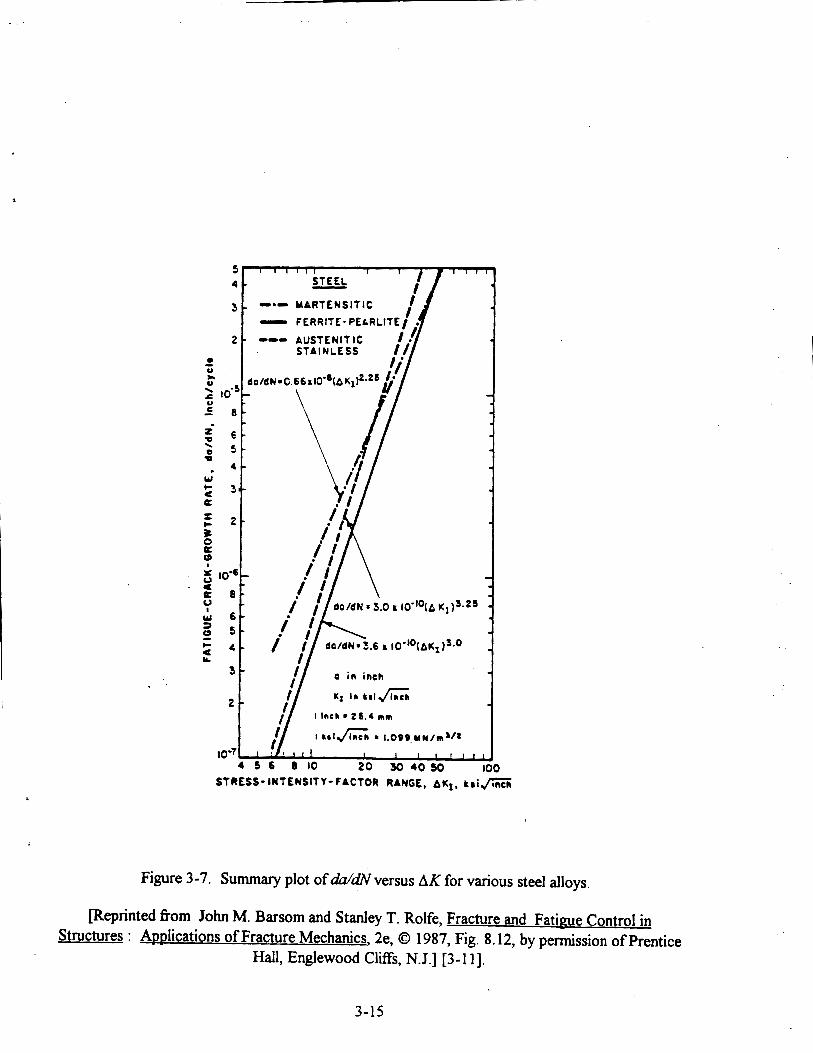
Figure 3-7. Summary plot of &&versus AK for various steel alloys.

meprinted fiom John M. Barsom and Stanley T. Rolfe, Fracture and Fatigue Control in Structures : Applications of Fracture Mechanics, 2e, 0 1987, Fig. 8.12, by permission of Prentice

Hall, Englewood Cliffs, N.J.] [3-111.

3-15

Figure 3-8. Summary plot of WdNversus AK for five titanium alloys.

[Reprinted from John M. Barsom and Stanley T. Rolfe, Fracture and Fatigue Control in Structures : Applications of Fracture Mechanics, 2e, 01987, Fig. 8.14, by permission of Prentice

Hall, Englewood Cliffs, N.J.][3-111

3-16

‘oor-=E333 2 . 5 ~ 1 0-lo(w4 BASED ON R = 0

7075-T6 AI, 0.090 IN. SHEET, CC SPECIMENS, L-T DIRECTION Environment Specimen Thk.: 0.090 in.; Width: 12.0 in. Reference No. : 75599, 79804

: 70 F, Lab Air; Frequency: 0.5 to 30 Hz

(a) Results for R = 0 and R = 0.2.

Figure 3-9. 7075-T6 aluminum (0.09 in. thick) crack growth rate properties.

,

Beprinted fiom Damage Tolerant Design Handbook, 1975, Fig. NAR4, by permission of Battelle, Columbus, Ohio.] [3-121

3-17

2.5~10-’(AK)~ 1-R

3.35~10-*~(hK)~ I-R ..

z TI 2: m N

TI v

c 0 c,

m

0 L

.r

m m n

n

Stress Intensity Factor Range, AK, ksi-in.”2

: 70 F, Lab Air; Frequency: 0.5 to 30 Hz 7075-T6 AI, 0.090 IN. SHEET, CC SPECIMENS, L-T DIRECTION Environment Specimen Thk.: 0.090 in.; Width: 12.0 in. Reference No. : 75599.798Oa

@) Results for R = 0.33 and R = 0.5.

Figure 3-9 (continued). 7075-T6 aluminum (0.09 in. thick) crack growth rate properties.

[Reprinted fiom Damage Tolerant Design Handbook, 1975, Fig. NARS, by permission of Battelle, Columbus, Ohio.] [3-121

3-18

E .r

m- N

U

aJ +I m U c 0 *.)

Y

..

.l-

m 0)

0 L

m n

n

0 m L

I IO Stress Intensity Factor Range, AK, ksi-in."*

7075-T6 AI, 0.090 IN. SHEET, CC SPECIMENS, L-T DIRECTION Environment: Specimen Thk. : 0.090 in.; Width: 12.0 in. Reference No. : 75599. 79804

: 70 F, Lab Air; Frequency: 13.7 Hz

(c) Results for R = 0.7 and R = 0.8.

Figure 3-9 (continued). 7075-T6 aluminum (0.09 in. thick) crack growth rate properties.

,

, 1 0 - 9 ( ~ ~ ) 4

1-R

7 . 5 ~ 1 O - ' O ( A K ) ~

1-R

meprinted fiom Damage Tolerant Desim Handbook, 1975, Fig. NAFt6, by permission of Battelle, Columbus, Ohio.] [3-121

3-19

Similar procedures have been followed in Figure 3-9(b) and (c), except that the Walker 1-R factor

has also been used to correct the raw rate constant obtained from the plots:

Stress ratio, R 0 0.33 0.5 10'O c 2.5 3.35 25.0

(1 - R)(Raw value) 2 C =

0.7 0.8 7.5 10.0

(3-14)

The raw value is the C obtained directly fiom the intercept as given in equation (3-13). The

results shown in the right hand border are for the corrected rate constant C.

The table below compares the results obtained fiom Figure 3-9 and shows that some anomalies

exist. For example, C for R = 0.5 is much larger than the rate constant obtained for the other

stress ratios. Is this a real effect? Closer examination of Figure 3-9(b) casts some doubt on the

validity of the high value. The curve fitter's eye was obviously attracted to the series of data

points at R = 0.5 between AK = 5 and AK = 15 hi f i . This group is isolated from the clutter and seems to characteke the R = 0.5 behavior. Conversely, upon close examination, one can

distinguish many more R = 0.5 data points in the R = 0.33 scatter band. Therefore, the analyst

might reasonably discard the R = 0.5 curve fit and work with the results fiom the other stress

ratios.

Summary of results for rate constant C obtained fiom Figure 3-9.

Even without the R = 0.5 result, the spread in the other values for C shows that the Walker

equation does not fit this group of data very well. A good fit should produce C values within 10

percent of each other, in order to allow the use of a group average. Conversely, the spread in the

above table is a strong warning against extrapolation. If a Walker equation is used, the rate

constant should be selected to match the stress ratios expected in the structure when the equation

is applied.

3-20

On the other hand, the data group (except for R = 0.5) can be reasonably well represented by the

modified Walker equation:

Stress ratio, R 10'O c

(3-15)

0 0.33 0.7 0.8

2.5 2.37 2.66 2.5 1 AVG= 2.5

The value C = 2.5 x lo-'' is obtained in this case by modifjing equation (3-14), after trial, to the

form:

(3-16)

with the results shown in the table below.

How reliably can any of the WiNequations derived above represent 7075-T6 thin sheet? Aside

fiom the doubtfil curve fit for R = 0.5, the results appear to come fiom two test series, and the

number of data points is quite large. On the other hand, Figure 3-10 shows two 7075-T6 data

sets for somewhat thicker sheet from a different test series. In this case, the C value based on the

R = 0.2 data is at least three times the value obtained fiom the preceding data reduction, and at

R = 0.5 the results agree with the preceding "anomalous" result! This kind of situation can only

be resolved by going back to the data sources to check for errors or procedural differences, or by

getting more data. The lesson to learn fiom this example is to compare crack growth rate data

from as many independent sources as possible.

. -

Figure 3-1 l(a) through (d) presents a series of plots for 2024-T3 thin sheet at four different stress

ratios. The plots in Figure 3-1 l(a) come fiom a different test series than the other plots, and the

two values R = 0.1 and R = 0.1 1 are considered to represent the single stress ratio R = 0.1 for

- Stress Frequency, No. of No. of 1 - Ratio. R 1. Hz Specimens Data Points / 1

I / w k 0 0.020 3.00 4 36 /

K)" 0 0.500 3.00 5 34 r 1-R E // E3 8 . 5 ~ 10-10(AK)4 AT R r O

I I l l J I IO 100 200

Stress Intensity Factor Range, AK, ksi- in!R

7075-T6 AI, 0.20 IN. SHEET, CC SPECIMENS, L-T DIRECTION Environment : 70 F, Lab Air Specimen Thk.: 0.200 in.: Width: 11.50 in. Reference No. : 86088

Figure 3-10. 7075-T6 properties (0.2 in. thick) from a different test series.

Beprinted from Damage Tolerant Desim Handbook, 1975, Fig. NAR7, by permission of Battelle, CoIumbus, Ohio.] [3- 121

3 -22

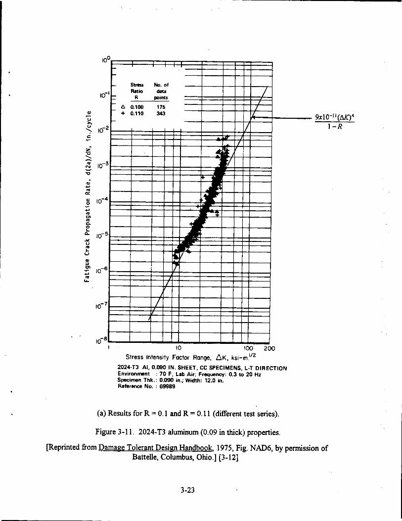
V h V \ c .I- .. z 0

m N Y

c, m tn

0 L a

m n

Y V m L u

strarr No.of h i 0 data

A 0.100 175 + 0.110 343

I 10 100 2 0 0 Stress Intensity Factor Range, AK, ksi-rn.”2

2024-T3 AI, 0.090 IN. SHEET, CC SPECIMENS, L-T DIRECTION Environment Specimen Thk.: 0.090 in.; Width: 12.0 in. Reference No. : 69989

: 70 F, Lab Air; Frequency: 0.3 to 20 Hz

(a) Results for R = 0.1 and R = 0.11 (different test series).

9x 1 0-l (AQ4 1 -R

Figure 3-1 1 . 2024-T3 aluminum (0.09 in thickj properties.

[Reprinted from Damage Tolerant Design Handbook, 1975, Fig. NAD6, by permission of Battelle, Columbus, Ohio.] [3-121

3-23

m m n cn

0 L

Y V L u 0) 3 cn

'* c, m LL

m

Stress Intensity Factor Range, AK, ksi-in."2

Environment : 70 F, Lab Air; Frequency: 20 to 30 Hz Specimen Thk.: 0.090 in.: Width: 12.0 in. Reference No. : 75599, 79804

2024-T3 AI, 0.090 IN. SHEET, CC SPECIMENS, L-T DIRECTION

(b) Results for R = 0.33.

Figure 3-1 I(continued). 2024-T3 aluminum (0.09 in. thick) properties.

3 . 3 5 ~ 1 0 - ' ~ ( h K ) ~ l - R

[Reprinted fiom Damage Tolerant Design Handbook, 1975, Fig. NAD7, by permission of Battelle, Columbus, Ohio.] [3-121

3 -24

c .r

c 0 .r c, m cn

0 L

A! V m L V

m n

m m a -I- C, m U

Stress No. of Ratio data

a 0.500 130

IO Stress lntenslty Factor Range, AK, ksl-In

2024-T3 AI, 0.090 IN. SHEET, CC SPECIMENS, L-T DIRECTION Environment : 70 F, Lab Air; Frequency: M to 30 Hz Specimen Thk.: 0.090 in.; Width: 12.0 in. Reference No. : 75599, 79804

(c) Results for R = 0.5.

Figure 3-1 1 (continued). 2024-T3 aluminum (0.09 in. thick) properties.

- 2.5~10-~O(AK)~ 1-R

[Reprinted fiom Damage Tolerant Desim Handbook, 1975, Fig. NADS, by permission of Battelle, Columbus, Ohio.] [3-121

3-25

W

m QI m p. 0 L

Y V m L V

W ‘ S

ml

Stress No. of 10-1 Ratio data

A 0.700 106

10-2

IO-^

IO-^

10-5

10-6

loo 200 I b 8

I IO Stress Intensity Factor Range, OK, ksi-in ‘’*

Environment : 70 F, Lab Air; Frequency: 13.7 Hz Specimen Thk.: 0.090 in.; Width: Reference No. : 75599.79804

2024-T3 AI, 0.090 IN. SHEET, CC SPECtMENS, L-T DIRECTION

12.0 in.

1 .5~10- ’~(hK)~ 1-R

(d) Results for R = 0.7.

Figure 3-1 1 (continued). 2024-T3 aluminum (0.09 in. thick) properties.

[Reprinted from Damage Tolerant Design Handbook, 1975, Fig. NAD9, by permission of Battelle, Columbus, Ohio.] [3-121

3-26

practical purposes. Again, lines with the rate exponent m = 4 have been drawn on each plot, and

the table below summarizes the corresponding rate constants C for a Walker equation. In this

case, there is no trend which could be used to fit the data with a modified Walker equation, and

the values spread too much to justify a group average. In the absence of additional independent

data, one might make a conservative judgment by choosing a value between 2.5 x lo-’’ and

3 x for C.

Summary of rate constants obtained from Figure 3- 1 1.

I 1 O’OC I 9 1- 3:35 I 2.5 I 1.5 1

Another important feature of the data in Figure 3-1 l(c) through (d) is the appearance of wide

scatter bands in the accelerated growth region. If a Forman equation is needed to represent this

region for damage tolerande analysis, the curve fit will be unreliable, and the only reasonable

choice would be to adopt a very conservative (i.e., low) value for the K, parameter. This is

another example where it would be better to recheck the data source and seek additional

independent data. .

Figure 3-12 shows a plot of data at R = 0 for 1/4-inch thick 2014-T6 sheet from a single test

series. Note that there are very few points in the slow growth region, making it difficult to fit the

data properly. Two possible lines have been drawn on the plot:”

(3-17)

(3-18)

Either equation represents the data well in the region where the data points lie, but either equation

can also give unconservative (low) rates outside that region, depending on whether extrapolation

is made toward higher or lower AK.

Note also that the dddN rates are plotted, i.e., the correction factor of 2 is not required here. 10

3-27

I00 Stress Frequency, No. of No. of

Ratio, R 1, Hz Specimens Data Points

lo-'

K 0

c, m m m 0 L Q

.r

n

I IO loo 200 Stress Intensity Factor Range, AK, ksi-in."*

2014-T6 AI, 1.00 IN. ROLLED BAR, CC SPECIMENS, L-T DIRECTION Environment : 70 F, Lab Air Specimen Thk.: 0.25 in.; Width: 7.50 in. Reference No. : 86213

5x1 O - ' 2 ( ~ 5 . 3

6x1 O-" (AK)~

,

Figure 3-12. 2014-T6 aluminum (0.25 in. thick) properties at R = 0.

[Reprinted from Damape Tolerant Design Handbook, 1975, Fig. N U S , by permission of Battelle, Columbus, Ohio.] [3- 121

3-28

This example shows why it is important to be aware of the general properties expected for an

alloy class. Based on aluminum alloys as a class, one would tend to suspect the validity of

equation (3-17) because of its abnormal m value. Indeed, comparison with independent data for a

different thickness supports the selection of the curve fit based on m = 4 (see Figure 3-13).

In the preceding examples, it has sometimes been necessary to compare data fiom tests of

specimens having different thickness in order to expand the base of independent results. Such

comparisons are most usehl for the purpose of establishing a reliable rn value. Conversely,

considerable care should be exercised in comparing C values. In particular, one should not

attempt to establish C based on a group average fiom tests of different thickness ifthe individual

values are spread out, since the spread may reflect an actual trend.

Figure 3-14(a) illustrates the thickness effect trend in 7475-T651 plate. The rate constant C

increases as the thickness in’creases, until the plate is thick enough to be valid for plane strain

fracture. The transition fiom thin-sheet properties to plane strain properties is reflected by a

factor of 3 in the rate constant.

Figure 3-14(b) illustrates another important effect: corrosive environments. The dry air test

condition (slightly more favorable than ambient or high-humidity air) is generally used as a

baseline for comparing environmental effects. The 3.5% salt solution is a generally accepted

representation for saltwater and moisture trapped fiom marine environments. For the alloys

shown in the figure, the corrosive medium increases the rate constant by a factor of 2 to 3,

relative to the baseline condition. This phenomenon is called corrosion fatigue or environmentally

accelerated crack growth. The severity of corrosion fatigue depends strongly on the alloy

composition and temper,” and tests are essential to establish the magnitude of the effect for a

specific alloy. In order to operate, the corrosion fatigue mechanism requires a steady circulation

of the fluid medium near the crack tip to replenish the chemicals consumed by environmental I

Newer aluminum alloys such as 7175-T73 have been adopted for aircraft construction in part because they are 11 ’ less prone to corrosion fatigue than older alloys such as 7075-T6.

3-29

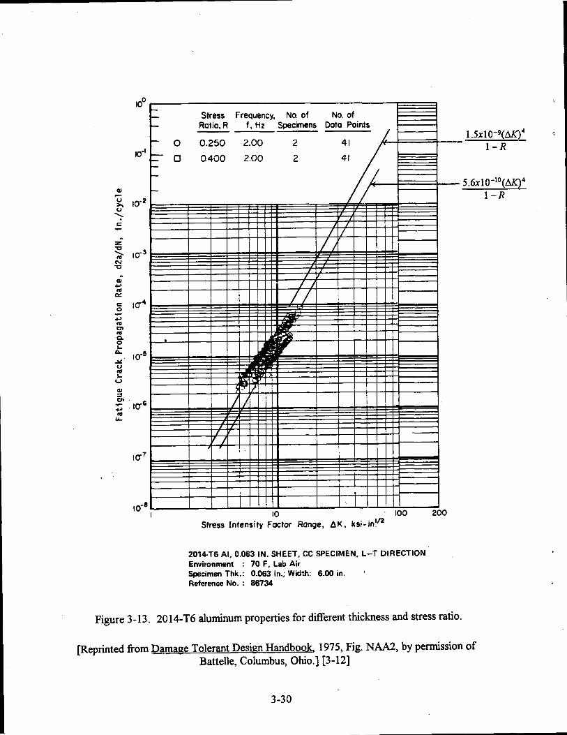
IO0

IO"

10-2

I I I I l l l l l I I + I I I I

lo-'

I

Id8

- I - Ratio, R f, Hz Specimens Data Points - - Stress Frequency, No. of No. of t

1 . ~ x ~ O - ~ ( A K ) ~ 1-R - 0 0.250 2.00 2 41

0 0.400 2.00 2

Stress Intensity Factor Range, AK, ksi-in!/2

2014T6 AI, 0.063 IN. SHEET, CC SPECIMEN, L-T DIRECTION Environment : 70 F, Lab Air Specimen Thk.: 0.063 in.; Width: 6.00 in. ' Reference No. : 86734

Figure 3-13. 2014-T6 aluminum properties for different thickness and stress ratio.

[Reprinted fiom Damage Tolerant Design Handbook, 1975, Fig. N M , by permission of Battelle, Columbus, Ohio.] [3-121

3-30

10

. -

(a) Effect of thickness on FCP behavior of 7475-T65 1 machined fiom 1 -inch plate (b) A comparison between the FCP rates

I in dry air and 3.5% NaCl solution for and tested in dry air. . -

I

aluminum alloys.

FCP: Fatigue Crack Propagation

Figure 3-14. Effects of thickness and environment.

Reprinted fiom Damage Tolerant Desim Handbook, 1975, Figs. NAW48 and NAW49, permission of Battelle, Columbus, Ohio.] [3-121

3-3 1

attack. Thus, corrosion fatigue generally occurs only when the frequency of fatigue loading is

below 10 Hz, i.e., when the crack remains open long enough to allow fluid circulation.

C (English units) = (1,099)m C (SI units) 0.0254

All of the examples in this section are based on data plots in English units (idcycle for crack growth rates and ksi& for stress intensity factors). However, evaluations in the fbture may require comparison of English-unit data with results presented in Systeme Internationale (SI)

units. The following conversion factors are useful for this purpose:

(3-20)

Crack growth rate: 1 idcycle - - 0.0254 dcycle

6.895 MPa - Stress: 1 ksi -

Stress Intensity Factor: 1 ksi f i - - 1.099 MPa f i

(3-19)

SI-unit stress intensity factors may also be reported as MN-m3n , a unit identical to MPa f i . Special attention must be paid to conversion of rate constant because the conversion factor

depends on th? rate exponent m:

3.4 CRACK GROWTH LIFE ESTIMATES

Crack growth life estimates are made for one oftwo general purposes. Some components are

restricted to a single load path for practical design reasons. In such cases, the purpose of the

estimate is to demonstrate that the slow crack growth life exceeds the component service life by a

suitable factor of safety. Other components have multiple load paths for fail-safety and can

tolerate the loss of one path due to fracture. In such cases, estimates are required to establish

when to begin periodic inspection and the length of the interval between inspections. Inspection

intervals are based on the time required for the largest crack which may escape detection to grow

to a size which can be expected to cause a fracture during the next flight. The inspection interval

3-32

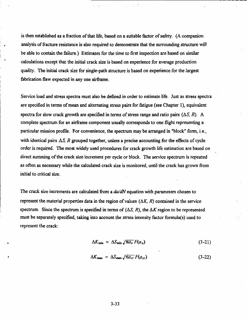
is then established as a fraction of that life, based on a suitable factor of safety. (A companion

analysis of fiacture resistance is also required to demonstrate that the surrounding structure will

be able to contain the failure.) Estimates for the time to first inspection are based on similar

calculations except that the initial crack size is based on experience for average production

quality. The initial crack size for single-path structure is based on experience for the largest

fabrication flaw expected in any one airframe.

Service load and stress spectra must also be defined in order to estimate life. Just as stress spectra

are specified in terms of mean and alternating stress pairs for fatigue (see Chapter l), equivalent

spectra for slow crack growth are specified in terms of stress range and ratio pairs (AS, R). A complete spectrum for an airfiame component usually corresponds to one flight representing a

particular mission profile. For convenience, the spectrum may be arranged in "block" form, i.e.,

with identical pairs AS, R grouped together, unless a precise accounting for the effects of cycle order is required. The most widely used procedures for crack growth life estimation are based on

direct summing of the crack size increment per cycle or block. The service spectrum is repeated

as often as necessary while the calculated crack size is monitored, until the crack has grown fiom initial to critical size.

The crack size increments are calculated from a MdZV equation with parameters chosen to

represent the material properties data in the region of values (AK, R) contained in the service

spectrum. Sine the spectrum is specified in terms of (AS, R), the AK region to be represented must be separately specified, taking into account the stress intensity factor formula(s) used to

represent the crack:

(3-21)

(3 -22)

3-33

where AS-, AS,, are the minimum and maximum stress ranges in the spectrum, a. is the initial crack length, and a, is the critical crack length. The stress intensity factor solutions for various

geometries are available in handbooks [2-6 to 2-91. Some typical examples are also included in

Appendix A.

Attention should also be paid to the possibility that the MdiV equation might be inadvertently

extrapolated beyond its applicable region in the stress ratio variable. If a Walker, modified

Walker, Forman or similar equation is used, unconservatively low crack length increments can be

projected for cycles that have R < 0 (compressive minimum stress), a condition that is not

normally tested in the laboratory because of the problems created by grip slack. Spectrum cycles

with R 0 should not normally occur except in the ground-air-ground cycle. Nevertheless, it is a

good idea to adopt the conservative procedure of preprocessing the spectrum to truncate negative-R cycles to R = 0 (and A S = AS- to correspond)."

m

Various procedures with different degrees of numerical approximation are used to calculate

spectrum crack growth life. The direct sum (cycle-by-cycle) method has no approximations and

serves as a baseline. In this method, the crack length increment A a is calculated for one stress

cycle and the crack length is immediately updated to a + A a for the next cycle. This is also the method most easily adapted to deal with load interaction effects (see Section 3.5).

In the direct sum (block method), the spectrum order is disregarded, and the stress cycles are

grouped into blocks [(n,, AS,, R,); (n, AS2, RJ; ...( nD ASJ, RJ)], i.e., the flight is considered to

consist of n, cycles with stress range AS, and stress ratio R,, etc. Crack length increments

Aa,, Aa,, etc. are calculated for each block before updating the crack length. Based on the

"The pre-processor should also scan for and delete any cycle for which both S, and S, are compressive. Such cycles can occur in taxi loads. They do not actually contribute to crack growth, but leaving them in the spectrum may introduce large errors in calculated crack growth. Compression cycles are insidious because they can have positive R values much greater than 1, leading to an artifact of "negative crack growth."

3-34

. .

r

.I

,

Walker equation, for example, the sequence of calculations starting fiom the initial crack length

would be as follows:

al,ao + nl(-) da dN

(3-23)

and so forth.

Another variation of this procedure is the direct sum (spectrum) method, in which the crack

length is only updated after each full spectrum. In this case, the calculation can be done more efficiently by factoring out the crack length terms as common terms in the expression for Aa for one complctespectrum:

(3-24)

Note that, since the sum of stress spectrum terms does not depend on'crack length, it need be

calculated only one time.

The direct sum (block) and direct sum (spectrum) methods are prone to lag because the crack

growth rate is progressively underestimated in the second and succeeding stress cycles. Updating

3-35

the crack length at the end of each block or spectrum reduces but does not eliminate the lag. The

error may be insignificant over a few flights but may accumulate to an unconservative level if a life

in the range of lo3 to lo5 flights is being calculated. When these direct sum methods are being

used in such applications, the lag error should be evaluated by comparing the results for a typical

case with results calculated by the direct sum (cycle-by-cycle) method.

The equivalent S-N curve method is an alternative approach that is usehl for checking other

results or looking at the effect on life of changes in design or service variables. The basic concept

of the method is to use the for each block equation to calculate a constant-amplitude life

(nj , A,!$ R,> in the spectrum. In other words, N, is the total number of cycles of (AS,, R,) that would be needed to make the crack grow from the initial length a. to the critical length a,,,

assuming that only (A,!$, RJ cycles are applied. The spectrum crack growth life is then estimated by applying Miner's rule:

b

1 Life (number of flights) = J

j = 1 C (njlq)

(3-25)

The equivalent S-N curve method receives its name from its resemblance to the way in which the

older safe-life calculations were made, based on S-N fatigue curves. The method was put to

widespread-use by the Air Force Logistics Command (AFLC) in the 1970s when the Air Force

began to apply damage tolerance assessment retrospectively to Its existing aircraft fleets. The

AFLC adopted the equivalent S-N curve method primarily because it was the easiest way to

modi@ their maintenance scheduling software, which had been based on S-N fatigue life and

Miner's rule.

If the constant-amplitude crack growth lives A$ are accurately calculated, then the only numerical

error in the equivalent S-N curve method comes from spectrum sequence effects. This source of

error can be understood by considering what would happen to a crack subjected to a spectrum

consisting of only two stress ranges, one small and one large, with enough cycles of each so that

3-36

the entire crack growth life only takes one or two spectra. Under these circumstances, that actual r crack growth life would be short if the large-amplitude cycles were applied first and long if the

small-amplitude cycles were applied fkst. The equivalent S-N curve method gives an answer

between these two extremes. Fortunately, this type of sequence error becomes insigntficant in

practical cases where the sequence of stress cycles in the spectrum is well mixed and the actual

crack growth life ranges from 1 O3 to 1 Os flights.

s

3.4.1 Quick Estimates with Crack Geometry Sums

The equivalent S-N method can also be used to make quick estimates of crack growth life.

Estimates are sometimes usehl for evaluating the effects of design trade-offs. For example,

suppose a crack is modeled by K = S J E F ( a ) and the life to grow the crack from a, to a2 is sought. The material is represented by a Walker equation:

and the loading is specified as a spectrum (nj, Aq., RJ.

Suppose that the total crack growth a2 - a, is divided into a large number M of small steps:

a2 - a, = MAa

The spectrum crack growth rate,

3-37

can be expressed at each step as follows: )i

da = CCs [I JEiiiF(al)]" aw when a = a1

&= aw C & [ J m F ( a l + A a ) ] m w h e n a = a , + A a

aw = C & [ J w F ( a l + 2Aa)]" when a = al + 2 A a

and so forth. The time required for each step can then be approximated as Aa divided by the average of the rates at the beginning and end of the step, and the approximate total time

is the sum:

The quantity in brackets is called a crack geometry sum, since it contains all of the geometrical effects from the stress intensity factor model, independent of the stress spectrum sum, CS .

3.5 INTERACTION EFFECTS AND RETARDATION MODELS

The cycle order in a stress spectrum can influence crack growth life in a manner similar to its

effect on fatigue life. This phenomenon is called load or stress interaction, a tern which reflects

the fact that the rate of fatigue damage or crack growth during a particular cycIe depends not

only on the stresses in that cycle, but also on the stresses in earlier cycles. Neither the standard

laboratory crack grovhh rate tests nor the associated rate equations ,and life estimation methods

account for load interaction.

3-38

c

The discovery of load interaction effects in fatigue was quickly followed by a similar finding for

crack propagation [3-14, 3-15]. The basic crack growth experiments dealt with the eff'ects of an

isolated overload. When an overload was introduced in the midst of a constant-amplitude test,

the rate of crack propagation in the succeeding cycles was observed to drop sharply and then to

return gradually to the undisturbed value. This particular phenomenon was called retardation; the

term was later extended to cover observations of any spectrum crack growth tests in which the

measured life was consistently longer than the life estimated by means of one of the basic rate

equations.

Retardation models were developed for the adjustment of life estimates to reflect load interaction

effects. The first model was based on a purely empirical approach of establishing a scale factor

from spectrum test data [3-161. Since the scale factor was sensitive to changes in the stress

spectrum and crack geometry, this model proved to be a poor predictor and soon fell out of favor.

It was replaced by the Willenborg model [3-171, in which the first attempt was made to base the

retardation adjustment on physical grounds.

The Willenborg model is based on the fact that an isolated overload creates an enlarged plastic

zone ahead of the crack tip and the idea that the plastically deformed material reduces the rate of

crack growth through the zone. Let SOL denote the peak stress in the overload cycle and define

the overload plastic zone size as:

(3-26)

where KoL is the stress intensity factor corresponding to SOL and Y is the material yield strength.

Let Aa be the amount by which the crack has grown fiom the overload cycle to the current cycle

(S-, S-) and define the effective maximum stress for the current cycle as:

3-39

(3-27)

where S,ed is an empirically chosen parameter.I3 The crack length increment for the current cycle

is then calculated by substituting the corresponding parameters AKdand R,in the basic rate

equation. This procedure is followed until the crack grows completely through the overload zone

(h = rp) or another overload cycle is encountered. In the second case, a new overload plastic zone is calculated, and the effective stress procedure is restarted.

In spite of its empirical features, the Willenborg model was at least based on a reasonable physical

concept, and experience in applying the model showed that it was better able to simulate spectrum

retardation than the earlier model. The Willenborg model was also naturally suited for

incorporation into computer programs which estimate life by direct summation of crack length

increment per cycle or block.

The most realistic retardation model developed to date is the so-called crack closure model

proposed by Elber [3-1'8,3-19] and hrther developed by Newman [3-201. Elber's model is based

on the concept of stress reversal in the crack tip plastic zone. Under load, the material in the

plastic zone yields in tension and, under some conditions, may reverse its stress state to

compression when the load is removed. A residual state of compression near the crack tip can

keep the crack closed during the first part of a subsequent loading cycle, until sufficient externally

applied tensile stress, Sop, is imposed to re-open the crack. It is then reasonable to argue that the

rate of crack growth should be proportional to an effective stress intensity factor range, Kef, associated with the effective stress range AS# = S- - Sop rather than the nominal range

A S = S,, - S- . It can also be argued that Elber's model naturally incorporates the stress ratio effects observed in the standard laboratory tests, and thus, that only a Paris equation need be

used to describe basic crack growth rate properties at stress intensities below the accelerated

region.

The crack closure model requires a numerical analysis of elastic-plastic stress states in the vicinity of the

crack tip. A line-spring model of the plastic zone is used for this purpose, together with the assumption

The reduction stress S , must be specfied. It can be established by fitting the model to the results of isolated overload 13

tests.

3-40

that the zone is confined to the crack plane [3-201. The individual spring elements are

represented by elastic - perfectly plastic characteristics with a flow stress determined fiom the

material tensile strength properties. The model is subjected to enough cycles to represent the

plastic zone residual stress state, and the crack tip is then advanced to represent growth. The

spring elements cut by the advancing crack are left in the model to represent the plastic zone

wake, and new elements are added to extend the plastic zone itself. Additional cycles are then

applied, with the cut elements either in compression or stress-fiee, to analyze the state of crack

closure. At the beginning of each new cycle, a part of the calculation defines the value of Sop for

the cycle.

The crack closure model is able to make reasonable predictions of retardation in cracks growing

under spectrum loads, but the calculations are much more involved than those required for the

Willenborg model. In practice, the computing burden is often reduced by running the crack

closure calculation infrequently, on the assumption that any trend of opening stress associated

with increasing crack length is slow.

b

Another practical problem is that the closer calculations are extremely sensitive to small errors in

the elastic solution for the distribution of deformations near the crack tip (these deformations

control the behavior of the model spring elements). Consequently, good numerical results require

either an exact solution or a numerical solution with displacements computed for at least 20 to 30

points within one plqtic zone length along the crack surface.

3-41

3-1.

3-2.

3-3.

3-4.

3-5.

3-6.

3-7.

3-8.

3-9.


Paris, P.C. "The Growth of Fatigue Cracks Due to Variation in Load," Ph.D. Thesis, Lehigh University, Bethlehem, PA (1962).

Clark, W.G., Jr., "Fracture Mechanics in Fatigue," ExDerimental Mechanics, September, 197 1.

Paris P. and Erdogan, F., "A Critical Analysis of Crack Propagation Laws," Transactions of -Y ASME p. 528, December 1963.

Walker, E.K., "The Effect of Stress Ratio During Crack Propagation and Fatigue for 2024-T3 and 7075-T6 Aluminum," Effects of Environment and Complex Load Histov on Fatime Life. Spec. Tech. Publ. 462, ASTM (1970), 1-14.

Omnger, O., Tang, Y.H, Gordon, J.E., Jeong, D.Y., Moms, J.M., and Perlman, A.B. Crack Propayation Life of Detail Fractures in Rails, DOT Transportation Systems Center, Cambridge, MA, DOT/FRA/ORD-88/13, December 1988.

Forman, R.G., Kearney, V.E. and Engle, R.M., "Numerical Analysis of Crack Propagation in Cyclically Load"ed Structures," Trans ASME. J Basic Eng 89,459-464 (1967).

Jaske, C.E., Feddersen, C.E., Davies, K.B., Rice, R.C., Analysis ofFatigue. Fatigue-Crack Propagation. and Fracture Data. NASA CR-132332 (November 1973).

Collipriest, J.E., An Experimentalist's View of the Surface Flaw Problem. North American Rockwell Report SD72-CE-12 (June 1972).

Collipriest, J.E, and Ehret, R.M., A Generalized Relationship Representing the Sigmoidal Distribution of Fatime Crack Growth Rates. Rockwell International Report SD74'CE-000 1 (March 1974).

I

3-10. Swift, T., Damage Tolerance Technolop. A Course in Stress Analysis Oriented Fracture Mechanics, Phase 11, Federal Aviation Administration.

3-1 1. Rolfe, S.T. and Barsom, J.M., Fracture and Fatigue Control in Structures. Applications of Fracture Mechanics, Prentice Hall, 1987.

3-12. Damage Tolerant Desim Handbook, Metals and Ceramics Information Center, Battelle Columbus Laboratories, Columbus, OH. MCIC-HE3-0 1 (1 975).

3-13. Courtney, T.H., Mechanical Behavior of Materials, McGraw Hill, 1990 (Data from C.M. Hudson, NASA TN-D5390, 1969).

3-14. Schijve, J., "Effect of Load Sequence on Crack Propagation Under Random and Program Loading," Engineering - Fracture Mechanics 5,269-280 (1 973).

3-42

3-15. Schijve, J.,"Observations on the Prediction of Fatigue Crack Growth Under Variable-Amplitude Loading," Fatigue Crack Growth Under Spectrum Loads, ASTM STP 595, American Society for Testing and Materials, Philadelphia, PA, 1976.

3-16. Wheeler, O.E., "Spectrum Loading and Crack Growth," Transactions of ASME, Journal of Basic Engineering 94, 18 1 - 1 86 (1 972).

3-17. Willenborg, J., Engle, R.M., and Wood, H.A., A Crack Growth Retardation Model Using an Effective Stress Concept, AFFDL-TM-71-1-FBR (1971)

3-18. Elber, W., "The Significance ofFatigue Crack Closure," Damage Tolerance in Aircraft Structures, ASTM STP 486, American Society for Testing and Materials, Philadelphia, PA, 1971.

3-1 9. Elber, W., "Equivalent Constant-Amplitude Concept for Crack Growth Under Spectrum Loading," Fatigue Crack Growth Under Spectrum Loads, ASTM STP 595, American Society for Testing and Materials, Philadelphia, PA, 1976.

3-20. Newman, J.C., Jr., "A Crack Closure Model for Predicting Fatigue Crack Growth Under Aircraft Spectrum Loading," Methods and Models for Predicting Fatigue Crack Growth Under Random Loadihg;, ASTM STP 748 (1 98 1).

. '

0 U.S. COVERNENT PRINTIHG OFFICf~993-500-428/80041 3-43

Reproduced by NTlS National Technical information Service U.S. Department of Commerce Springfield, VA 22 1 6 1

This report was printed specifically for your order from our collection of more than 2 million technical reports.

For economy and efficiency, NTlS does not maintain stock of its vast collection of technical reports. Rather, most documents are printed for each order. Your copy is the best possible reproduction available from our master archive. If you have any questions concerning this document or any order you placed with NTIS, please call our Customer Services Department a t (703)487-4660.

Always think of NTlS when you want: Access to the technical, scientific, and engineering results generated

by the ongoing multibillion dollar R&D program of the U.S. Government. R&D results from Japan, West Germany, Great Britain, and some 20

other countries, most of it reported in English.

NTlS also operates two centers that can provide you with valuable information:

The Federal Computer Products Center - offers software and datafiles produced by Federal agencies.

The Center for the Utilization of Federal Technology - gives you access to the best of Federal technologies and laboratory resources.

For more information about MIS, send for our FREE NTlS Products and Services Catalog which describes how you can access this U.S. and foreign Government technology. Call (703)487-4650 or send this sheet t o NTIS, US. Department of Commerce, Springfield, VA 221 61. Ask for catalog, PR-827.

Name Address

Telephone

- Your Source to US. and Foreign Government Research and Technology.

U.S. DEPARTMENT OF COMMERCE Technology Administration

National Technical Information Service Springfield, VA 22161 (703) 487-4650

*Pa941 34336*

*PO*

BIN: M I 37 10- 1 7-97 INVOICE: 502616 SH I PTO : PAYMENT: CSH*VORNG

I *a2622

Introduction Fracture Mechanics Fatigue Crack · PDF fileI Assessment Handbook , FAA Technical...

Documents

Transcript of Introduction Fracture Mechanics Fatigue Crack · PDF fileI Assessment Handbook , FAA Technical...