Intertemporal Content Variation with Customer Learning

Fernando Bernstein, Soudipta Chakraborty, and Robert Swinney∗

June, 2021

Abstract

Problem Definition: We analyze a firm that sells repeatedly to a customer populationover multiple periods. While this setting has been studied extensively in the context of dynamicpricing—selling the same product in each period at a varying price—we consider intertemporalcontent variation, wherein the price is the same in every period, but the firm varies the contentavailable over time. Customers learn their utility on purchasing and decide whether to purchaseagain in subsequent periods. The firm faces a budget for the total amount of content availableduring a finite planning horizon, and allocates content to maximize revenue.Academic/Practical Relevance: A number of new business models, including video stream-ing services and curated subscription boxes, face the situation we model. Our results show howsuch firms can use content variation to increase their revenues.Methodology: We employ an analytical model in which customers decide to purchase in mul-tiple successive periods, and a firm determines a content allocation policy to maximize revenue.Results: Using a lower bound approximation to the problem for a horizon of general lengthT , we show that while the optimal allocation policy is not, in general, constant over time, it ismonotone: content value increases over time if customer heterogeneity is low and decreases oth-erwise. We demonstrate that the optimal policy for this lower bound problem is either optimalor very close to optimal for the general T period problem. Furthermore, for the case of T = 2periods, we show how two critical factors—the fraction of “new” versus “repeat” customers inthe population, and the size of the content budget—affect the optimal allocation policy and theimportance of varying content value over time.Managerial Implications: We show how firms that sell at a fixed price over multiple periodscan vary content value over time to increase revenues.

Keywords: intertemporal content variation; revenue management; customer learning

1 Introduction

In recent years, a number of successful new business models, primarily services, have arisen that

incorporate the following combination of features:

1. Customers purchase (or experience service) from the firm repeatedly over successive periods.

2. The firm charges a fixed price for each purchase or service experience across all periods.

3. While the firm does not change the price from one period to the next, it can change the

content that it offers to customers in each period.

∗Bernstein and Swinney: Duke University, {fernando.bernstein@duke.edu, robert.swinney@duke.edu}.Chakraborty: University of Kansas, soudipta.c@ku.edu.

1

Two prominent examples are video streaming services and curated subscription boxes. Video

streaming services such as Netflix, Apple TV+, Hulu, and Disney+ provide customers access to a

catalog of content (typically films or television series, produced both in-house and by third party

production companies) for a monthly subscription fee. While the subscription fee is pre-determined

and seldom changes (Forbes 2019), the catalog is regularly updated by adding new content, i.e.,

by producing new movies and series or purchasing the broadcast rights to third-party content,

and by removing older content (Engadget 2018, Digital Trends 2020). Thus, customers purchase

repeatedly (they subscribe on a monthly basis, typically without an obligation to commit more

than one month at a time) at a fixed price for each purchase, but the content offered (the video on

the streaming service) changes on a continual basis.

Similarly, curation subscription box services ship unique collections of related physical goods

to customers at regular intervals, e.g., weekly or monthly, for a fixed, pre-determined, per-box

price. Examples of the types of items offered via this business model include meal kits (Blue Apron

and Hello Fresh), cosmetics and personal care items (Birchbox and Ipsy), and even pet products

(BarkBox). As with streaming video services, subscription box customers repeatedly purchase at

a fixed price per box received, while the firm may vary the box contents offered in each period.

The features illustrated in these examples stand in contrast to many traditional business models

that involve selling a fixed set of products over multiple periods, but at a price that changes

from one period to the next. This allows traditional firms to engage in dynamic pricing, i.e.,

to manipulate the price over time to maximize revenue, a practice that has received enormous

research attention in the last two decades (Talluri & Van Ryzin 2006). The service providers

in our examples, however, generally do not engage in dynamic pricing: rather, video streaming

and subscription box services have a different lever at their disposal, as they can allocate content

over time to influence customer purchasing decisions. We refer to this resource allocation problem

as intertemporal content variation, and this practice is precisely what we study as we seek to

understand how firms can optimally vary the content they offer over time—rather than price—in

order to maximize revenue.

To accomplish this, we analyze a stylized model of a service provider determining content over

multiple successive periods in a finite planning horizon. In each period, customers decide whether

to purchase based on the current content that is offered by the provider—e.g., the current set of

2

movies or TV series available on Netflix, or the current set of menu items on a meal kit service like

Blue Apron. A key element of the businesses in these examples is that their customers experience

multiple sources of utility. First, they experience some utility from the content that they gain access

to (i.e., the particular movies or series offered on a streaming service, or the items for a curation

subscription box). This utility is typically known to customers in advance of a purchase decision:

for instance, Netflix heavily advertises new movies and series before they are released, while meal

kit services list menus on their websites for the next several weeks.

However, beyond the utility for the content they receive, customers also experience some service

utility from receiving that content. Video streaming services do not just offer movies and TV series,

they also offer a user interface that helps customers navigate and select what to watch, personalized

recommendations for new content, and a convenient way of watching video (compared to purchasing

or renting physical media). Curation subscription services do not just offer the items in the box,

they also curate those items (search for novel and interesting items to offer), package them in

a box, and deliver them to the homes of customers on a regular basis. This “service” element

of customer utility is typically not known by new customers until they experience the service at

least once—for instance, a customer does not know whether they like the Netflix user interface

and content recommendation algorithm until they use Netflix—and thus it must be learned via a

service experience. Similarly, a meal kit customer can only find out whether they like Blue Apron’s

curation and delivery service by subscribing to it.

These dual sources of utility—content utility, which the firm can manipulate over time via its

content allocation decisions, and service utility, which is constant from one period to the next but

initially unknown to new customers—play important roles in the purchasing decisions of customers

as well as the content decisions of the service provider. For example, because they do not yet

know their service utility, new customers may need to be enticed to try the service by offering

exceptional content, such as a hit TV series or a trendy new recipe. This would seem to suggest

that the service provider could benefit from placing content of significant value early in the planning

horizon, encouraging many new customers to experience the service and learn their utility. However,

if the provider allocates all of its best content early on, customers may choose not to purchase in

subsequent periods, knowing that the remaining content is less appealing. Moreover, because of

their different needs and tastes, both components of utility will, in general, be heterogeneous among

3

customers.

What makes this problem especially challenging is the fact that service providers are resource-

constrained. Put concretely: if a streaming service could offer hundreds of hit new series and

movies each month, it would be able to attract many new subscribers and entice them to continue

as customers month after month. However, this would be prohibitively expensive, as the cost

of a television series can exceed $15 million per episode (for special effects heavy shows like The

Mandalorian on Disney+, but also for shows with highly paid stars like The Morning Show on

Apple TV+) while films can cost hundreds of millions of dollars. Since streaming services do not

have infinite resources to produce new content, they must operate within a budget, and allocating

more resources for new content in one month would mean less resources for others; in turn, while

this would raise demand for months with a high allocation of resources, it would result in lower

customer content utility and reduced demand in months with a lower allocation of resources.

This leads to our main research question: given the dual sources of customer utility and the

experiential nature inherent in service utility, how should a service provider allocate finite resources

over time to both attract and retain customers? To give a specific example using the case of a

streaming video provider: within a planning horizon (say, a fiscal year) should a streaming video

service release all its best new series and movies at once, should it spread them out equally over

time, or should it follow some other strategy? The service provider in our model thus faces a

constrained optimization problem with an exogenously specified total budget for content over a

planning horizon of T ≥ 2 discrete time periods. Customers dynamically choose in each period

whether to pay the service provider’s fee and access the content offered in that period based on

their assessment of the total utility, i.e., the sum of the content and service utility, in that period.

Customers are heterogeneous in both dimensions of utility; however, by allocating more of its

content budget to a period, the service provider can raise the average content utility in that period.

Using this framework, we determine how the service provider should allocate its content budget

to the individual periods over the planning horizon to maximize revenue. While the optimal allo-

cation policy for a problem with a general number of periods is challenging to derive analytically,

we propose a lower bound problem that adds constraints to the provider’s original optimization

problem and that is analytically tractable. We show that the optimal allocation policy to this lower

bound approximation is optimal to the original problem in a significant majority of cases and, even

4

when it is not, it results in a negligible loss in revenue. Interestingly, we find that, in general, the

optimal policy that results from this analysis does not necessarily consist of an equal allocation

of the content budget in every period; however, the optimal policy generally is monotone. The

critical factors that determine whether the optimal allocation increases or decreases over time, and

how much it deviates from an equal allocation, include the degree of customer heterogeneity, the

relative number of new and repeat customers, and the size of the content budget. Our results thus

show that these service providers can employ intertemporal content variation to influence customer

purchasing decisions, manipulate the rate of customer learning about their service utility, and in-

crease revenue, much like more traditional firms can dynamically vary prices from one period to

the next to improve performance, and we discuss conditions under which such content variation is

most (and least) important to the firm.

Our analysis proceeds as follows. In §2, we review the related literature. In §3, we describe the

details of our model. In §4 we examine the service provider’s optimal content allocation strategy

over a planning horizon of arbitrary length. In §5 we restrict attention to the case of a two period

horizon to generate further insights about how the composition of the customer population and the

size of the content budget affect the optimal allocation policy. §6 concludes the paper.

2 Literature Review

Our work lies at the intersection of several streams of research. The first is a stream of literature

in which demand in a period is dependent on various aspects of past interactions between a firm

and its customers such as service failure (Hall & Porteus 2000), price (Popescu & Wu 2007), sales-

force effort (Liu et al. 2007), capacity (Liu & van Ryzin 2011), fill rate (Adelman & Mersereau

2013), service level (Aflaki & Popescu 2014), etc. Many of these papers assume behavioral models

such as loss aversion, goodwill formation, and habituation to link the seller’s decision and the

customers’ actions between different periods. In Caulkins et al. (2006), a firm sells a good at a

fixed pre-determined price but can manipulate its quality over time. The quality choice determines

the seller’s reputation which in turn drives future sales. Another group of papers studies how parts

of an experiential service should be optimally sequenced to maximize the total perceived utility

of a customer (Verhoef et al. 2004, Dixon & Verma 2013, Dixon & Thompson 2016, Das Gupta

5

et al. 2016). The perceived utility depends on various behavioral effects like decreasing impatience,

satiation, and habit formation (Wathieu 1997, Baucells & Sarin 2007, 2010). In contrast to these

papers, we do not focus on any customer behavioral aspects; instead, in our model, the value of

content in the current period affects future demand in two ways. First, it determines how much

of the budget for content is left for the remaining periods. Second, once a customer signs up and

uses the service, he learns his service utility and makes future purchasing decisions based on this

realized utility and the value of the content in future periods. Hence, the provider optimally varies

the content value over time to influence the rate at which it gains new customers and the rate at

which it persuades existing customers to continue using the service.

The problem of how a firm should change its assortment of products during a selling season has

also been studied (Ulu et al. 2012, Caro et al. 2014, Bernstein & Martınez-de Albeniz 2017, Ferreira

& Goh 2020). Our paper is different than much of the assortment literature because the customers

in our model access the entire set of content and not individual products from an assortment.

Somewhat closer to our work is Caro & Martınez-de Albeniz (2020), who study how a content

creator can maximize traffic to a website by exerting costly effort over multiple periods to produce

new content. However, their model does not incorporate customer learning or an explicit model of

customer purchasing decisions, as our model does; rather, in their paper, customers arrive to the

website according to a Poisson arrival stream that is an increasing function of the content released

in a particular period. These modeling differences lead to very different results: for example, Caro

& Martınez-de Albeniz (2020) show that the optimal policy is to weakly increase content over time,

whereas we show that, depending on the degree of customer heterogeneity, it may be optimal to

increase or decrease content value over time.

Using a customer utility model that is somewhat similar to ours, Feldman et al. (2019) study

the quality decision of a firm selling a new experience good to customers who may strategically

delay a purchase to learn more information about quality. Hence, unlike Caro & Martınez-de

Albeniz (2020), they include both customer learning and an explicit model of customer purchasing

decisions, as we do; however, the situation they study is quite different from ours. For example,

we consider the optimal allocation of content across multiple periods with a fixed price, whereas

they model a one-time quality (and price) decision that is constant throughout the time horizon.

In addition, customers in our model decide whether to use the service in each period—and in

6

particular, customers may use the service multiple times within the horizon—while customers in

Feldman et al. (2019) buy the product at most once. Hence, while Feldman et al. (2019) do not

consider the issue of encouraging repeat purchases via the use of a time-varying content (or quality)

allocation policy, that is the focus of our paper.

To summarize, our model is the first, to our knowledge, in which a firm sells a non-durable good

that customers can repeatedly purchase at a fixed price over multiple periods, and the firm must

allocate a finite budget for the value of its product to each period in order to maximize revenue.

3 Model

In the following two subsections, we describe the decisions made by the two key sets of players in

our model: customers (in §3.1) and the service provider (in §3.2).

3.1 Customers

A service provider offers a set of content over a planning horizon consisting of T (≥ 2) periods.

In each period, customers can gain access to this content by paying an exogenous price p that is

constant throughout the planning horizon; as noted in the introduction, the prices for the types of

firms that motivate our model are typically long-term, strategic decisions that change infrequently

(Forbes 2018, USA Today 2019). Following our discussion in §1, each customer’s utility can be

divided into two additive parts: content utility and service utility. Customers are heterogeneous in

both components. Specifically, customer i’s content utility in period t is given by

vit = vt + εit, (1)

where vt is the mean utility derived from period t content, and εit ∼ N(0, σ2ε ) is a mean zero term

specific to customer i. We refer to vt as the value of the content, and it is this value that is chosen

by the provider when it chooses the content in each period (more on this choice will be discussed in

§3.2); hence, a higher value of vt results in higher average utility in the customer population. The

second term, εit, captures customer-specific heterogeneity in taste for the same content; higher σε

means customers have more heterogeneous tastes. At the beginning of every period, a customer

7

observes the content available for that period and his realized content utility vit. However, for

any customer i, εit is unobserved by the provider; hence, when choosing vt before period t, it only

relies on the distribution of εit in the customer population. Customer i’s realizations of εit are

independent across periods, which is appropriate if there is sufficient variety in the content from

one period to the next (i.e., different genres of TV series for a streaming video platform or different

types of cuisine for a meal kit service).

Customers are also heterogeneous in their service utility, θi, which is distributed over the cus-

tomer population as θi ∼ N(µ, σ2θ). This component includes all elements of customer utility

that do not originate from the provider’s content decisions, and thus depends on various inherent

features of the provider’s service (independent of the content) that are difficult to change in the

short-term. As a result, θi does not change from one period to the next, i.e., it does not depend

on t. Instead, it depends on how well these features match the idiosyncratic needs of a customer,

i.e., whether the customer happens to like the user interface of a streaming video provider or the

curation and delivery service of a subscription box provider. Hence, service utility differs from one

customer to the next, resulting in its distribution over the customer population and dependence

on i. Higher σθ means that customers have more heterogeneous valuations for the service. Putting

the two components—content utility and service utility—together, customer i receives total utility

(net of the purchase price) equal to

uit = θi + vt + εit − p (2)

from accessing the content of value vt in period t. Note that a portion of customer utility (θi)

is constant over time while another portion (εit) is i.i.d. in each period; while we have labeled

these components as belonging to “service” and “content” utility, respectively, they more generally

capture elements of customer utility that are persistent over time (θi) and elements that change

from one period to the next (εit). Depending on the distributions of these random variables, one

effect or the other (i.e., correlated or independent utilities over time) may dominate. We place no

restrictions on the parameter values p and µ.

Before customers have received service from the provider, they will not know how well the

provider executes that service nor whether it fits with their expectations; hence, before signing up

8

and using the service for the first time, customer i will not know θi beyond its distribution over

the population. We assume that after using the service for the first time, the customer perfectly

learns his service utility, θi. Mathematically, the customer observes his realization of total utility

in period t, uit, and using (2), infers his draw of θi = uit − vt − εit + p. In all subsequent periods,

the customer will know his realized service utility θi when making his purchasing decision. Just

as in the case of the content utility, the service provider cannot observe the realization of θi for a

particular customer, and instead uses its distribution over the customer population to determine

content.

We note here that it is possible that before signing up for the service, some components of

content utility might not be known to customers (e.g., customers who have never used a service

might be aware of only the more popular or heavily advertised items in the provider’s set of contents

in a period but not aware of the less popular ones), while they might know certain aspects of their

service utility (e.g., someone who has used a competitor service before will have a general idea of

his usefulness for the overall service category). Our model also extends to such situations as we

can relabel the component of customer i’s total utility that he knows before signing up in period t

as vit = vt + εit and all the remaining components, either from the the content or from the service,

that are revealed only after signing up as θi. The key features in the model are that some portion of

utility (regardless of its label) is only learned by customers after using the service, and the service

provider can increase the average utility of customers (again regardless of the label) by allocating

more resources to a time period.

All customers choose, in each period, whether they wish to access the content for that period

by paying the price p or not, and they incur no hassle cost for “pausing” or “restarting” their

service. In the examples discussed in §1, providers generally make it very easy for customers to

visit their website to sign-up or pause a service—e.g., it is nearly frictionless to pause and restart a

subscription for Netflix or Blue Apron. Customers are risk neutral with zero outside option value;

hence, a customer who has never used the service before will subscribe for the first time in period

t if E[uit|εit] = µ+ vt + εit− p ≥ 0. After receiving service at least once and observing θi, he would

subscribe again in a later period t′(> t) if uit′ = θi + vt′ + εit′ − p ≥ 0. Customers are assumed to

be myopic: they purchase in period t if and only if their net utility from period t consumption is

non-negative.

9

The market consists of a deterministic unit mass of infinitesimal customers, all of whom are

present at the beginning of the horizon. The assumption of infinitesimal customers is meant to

reflect the fact that the firms that motivate our study often have extremely large total customer

bases (i.e., active plus potential subscribers): as of 2020, Netflix, for example, has 195 million

active subscribers, while Disney+ has over 86 million, and thus the total customer base is even

larger. Hence, from the provider’s perspective, the customer population can be approximated by

a continuous mass. A fraction α ∈ [0, 1] of customers have used the service at some point in the

past (i.e., before period 1) and are aware of their service utility, θi. In other words, an α fraction of

the market are repeat customers while the remaining 1− α fraction are new customers, who have

never used the service before and need to purchase at least once to learn θi. As we will show in

§5, the relative sizes of these two segments of the customer population will play a critical role in

determining the firm’s optimal policy.

3.2 Service Provider

As noted previously, the price p for the service is exogenously specified and fixed throughout the

planning horizon. Similarly, the mean customer service utility, µ, depends on long term decisions

about the characteristics of the service (e.g., tools used for personalized recommendation, offline

download rules, number of parallel devices supported, parental controls, etc. for streaming services;

fulfillment capabilities, supplier quality, delivery partner quality, etc. for subscription boxes), and

is also exogenous and fixed for the duration of the planning horizon. This leaves content allocation

as the only remaining lever for the provider to influence customer purchasing decisions.

Creating content often comes with a significant leadtime: in the case of streaming services,

TV series and movies can take a year or more to produce, while subscription boxes must source

inventory for their boxes weeks or months in advance. Thus, before period 1, the provider decides

the contents for the entire planning horizon of T periods, consistent with the apparent policies of

the types of firms that motivate our study. For example, this planning horizon may be generated

by financial considerations (e.g., a fiscal quarter or year for a streaming video provider), or it may

be generated by the nature of the provider’s business (e.g., meal kit providers typically list menus

for the next 4-8 weeks to give customers time to make their decisions). Selecting the content for

all T periods at the beginning of the planning horizon implies an open loop optimization policy.

10

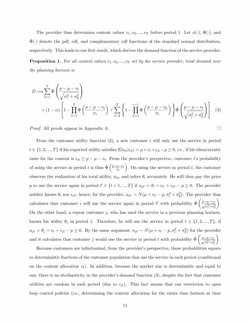
The provider thus determines content values v1, v2, ..., vT before period 1. Let φ(·), Φ(·), and

Φ(·) denote the pdf, cdf, and complementary cdf functions of the standard normal distribution,

respectively. This leads to our first result, which derives the demand function of the service provider:

Proposition 1. For all content values v1, v2, ..., vT set by the service provider, total demand over

the planning horizon is

D =αT∑t=1

Φ

p− µ− vt√σ2ε + σ2

θ

+ (1− α)

1−T∏t=1

Φ

(p− µ− vt

σε

)+

T∑t=2

{1−

t−1∏k=1

Φ

(p− µ− vk

σε

)}Φ

p− µ− vt√σ2ε + σ2

θ

. (3)

Proof. All proofs appear in Appendix A.

From the customer utility function (2), a new customer i will only use the service in period

t ∈ {1, 2, ..., T} if his expected utility satisfies E[uit|εit] = µ+vt+εit−p ≥ 0, i.e., if his idiosyncratic

taste for the content is εit ≥ p− µ− vt. From the provider’s perspective, customer i’s probability

of using the service in period t is thus Φ(p−µ−vtσε

). On using the service in period t, the customer

observes the realization of his total utility, uit, and infers θi accurately. He will then pay the price

p to use the service again in period t′ ∈ {t+ 1, ..., T} if uit′ = θi + vt′ + εit′ − p ≥ 0. The provider

neither knows θi nor εit′ ; hence, for the provider, uit′ ∼ N(µ+ vt′ − p, σ2ε + σ2

θ). The provider thus

calculates that customer i will use the service again in period t′ with probability Φ

(p−µ−vt′√σ2ε+σ2

θ

).

On the other hand, a repeat customer j, who has used the service in a previous planning horizon,

knows his utility θj in period 1. Therefore, he will use the service in period t ∈ {1, 2, ..., T}, if

ujt = θj + vt + εjt − p ≥ 0. By the same argument, ujt ∼ N(µ + vt − p, σ2ε + σ2

θ) for the provider

and it calculates that customer j would use the service in period t with probability Φ

(p−µ−vt√σ2ε+σ2

θ

).

Because customers are infinitesimal, from the provider’s perspective, these probabilities equate

to deterministic fractions of the customer population that use the service in each period (conditional

on the content allocation vt). In addition, because the market size is deterministic and equal to

one, there is no stochasticity in the provider’s demand function (3), despite the fact that customer

utilities are random in each period (due to εit). This fact means that our restriction to open

loop control policies (i.e., determining the content allocation for the entire time horizon at time

11

zero) is without loss of generality, as the service provider would not stand to gain from a closed

loop policy that adapts the content allocation after each period. However, we note that in practice,

complications might arise that could break this equivalence (e.g., non-infinitesimal customers, which

might be relevant for providers with smaller customer populations than those that motivate our

model, or stochastic arrivals of new customers in each time period).

The demand function (3) has an intuitive form. The first term, α∑T

t=1 Φ

(p−µ−vt√σ2ε+σ2

θ

), is the

demand from customers who know their utilities (i.e., θi) before period 1. Since these customers do

not need to learn θi by signing up, their purchasing behavior, and consequently, the form of their

demand functions will be identical in all periods. The second term captures the demand of customers

who do not know θi at the beginning of the planning horizon. The term 1 −∏Tt=1 Φ

(p−µ−vtσε

)is

the probability that a new customer uses the service at least once during the T periods. Hence,

this is the total mass of these initially new customers who sign up and learn their utility θi during

the planning horizon. The term Φ

(p−µ−vt√σ2ε+σ2

θ

)[1−∏t−1

i=1 Φ(p−µ−viσε

)]is the probability that a new

customer who has signed up between periods 1 to t−1 uses the service again in period t ∈ {2, ..., T}.

As noted previously, what makes this problem challenging is that the provider has finite re-

sources and cannot simply allocate very high content value in every period. To reflect this, we

introduce a budget V for the total value of content over a planning horizon of T periods. This

budget is infinitely divisible and the provider can allocate any value, vt ≥ 0 to content in period

t ∈ {1, 2, ..., T}, provided the total of the content over the T periods satisfies ΣTt=1vt ≤ V . It is easy

to see from (3) that a higher value of content in a period increases demand in that period. Hence,

the provider will always exhaust the total budget over the time horizon. Therefore, the provider

will choose the content values subject to the budget constraint:

ΣTt=1vt = V, where vt ≥ 0 ∀ t. (4)

The simplicity of the budget constraint allows us to analyze a complicated objective function

(derived in Proposition 1) while enforcing a key trade-off: the provider cannot offer highly valuable

content that results in high demand in every period, and hence it must allocate finite resources

to balance the rate at which it persuades new customers to sign up and repeat customers to use

the service again. Since items that are higher in value to customers should also be costlier for the

12

provider to offer (Mussa & Rosen 1978, Desai 2001, Jerath et al. 2017), we could also assign some

cost C per unit of content value, and then require that the provider maximize revenue subject to the

constraint that total content expenditure not exceed CV , i.e., that ΣTt=1Cvt = CV . Observe that

the cost C appears on both sides of this inequality; hence, we may think of the budget constraint

as a limit on the total operating cost of the service.

The provider’s objective is to maximize demand (3) subject to the budget constraint (4). We

let v∗t , t ∈ {1, 2, ..., T} denote the optimal content allocation over the planning horizon. Since the

price, p, is constant, maximizing demand is equivalent to maximizing revenue. Furthermore, we

normalize the marginal cost of fulfilling customer demand to zero, and hence maximizing demand is

also equivalent to maximizing profit. Note that if the service provider incurred a constant marginal

cost c for every unit of customer demand independent of the content allocation vt in a period,

maximizing profit (p − c)D would yield the same optimal solution as maximizing demand D. A

constant marginal cost might be the case if allocating more budget to a particular period means

increasing the variety (rather than the quality) of content offered (e.g., in meal kit services, offering

a broader or more diverse menu); if fulfillment or shipping costs are a large fraction of the marginal

cost of serving each customer and are independent of the precise contents offered in a period; or

if marginal costs are zero (e.g., first-party content on streaming services has no marginal cost for

each customer view, and providers often negotiate “lump-sum” licenses of third-party content that

do not require them to pay a fee for each customer view). However, in some instances, it might

be the case that the marginal cost of fulfilling customer demand depends on the precise content

offered in a period, i.e., it depends on vt; our model does not apply to this scenario.

To summarize, the firm solves the following optimization problem, where D is defined in (3):

Max D

s.t.

T∑t=1

vt = V (5)

vt ≥ 0, 1 ≤ t ≤ T.

The approach of maximizing demand subject to a fixed budget constraint is meant to reflect the

“flywheel” business model of Netflix and other similar start-up services: content is added to attract

customers, which generates cash, which then funds more content in subsequent years (Manjoo

13

2016). Our model approximates this effect by endowing the firm with a fixed budget (i.e., cash

generated from a previous planning horizon) that the firm uses to maximize demand and generate

the highest possible revenue (i.e., to fund the following planning horizon’s operations). As such, the

implicit assumption is that the budget is exogenous, and consequently the firm exhausts its entire

budget to maximize revenue. An extended version of our model might endogenize the budget itself

and maximize profit, i.e., revenue net of the budget, pD − CV , where C > 0 is a marginal budget

cost; we will discuss this extension in §6 of the paper.

4 Optimal Content Allocation

We now derive the optimal content allocation policy over a finite planning horizon. We first

observe that the standard deviation of θi, σθ, plays an important role both for the provider and

for customers. If σθ > 0, customers are heterogeneous in their utility from the value provided by

the service, and new customers are unaware of their total utility before period 1 and need to use

the service to learn it. To study the effect of this parameter on the provider’s optimal content

allocation, let us begin with the benchmark case of σθ = 0. In this case, the entire customer

population has the same utility, µ, from service and they all know this parameter accurately; as a

result, customers only differ in their idiosyncratic preference for content, εit. This extreme case has

a particularly simple optimal value allocation that serves as a useful benchmark for our subsequent

analysis.

In the remainder of the paper, we say that the optimal content allocation is increasing over

time when v∗t′ ≤ v∗t for all 1 ≤ t′ < t ≤ T , decreasing over time when v∗t′ ≥ v∗t for all 1 ≤ t′ < t ≤ T ,

and constant when v∗t′ = v∗t = V/T for all t′ and t. Note that the first two definitions are in the

weak sense. Given these definitions, we have the following result:

Proposition 2. When σθ = 0, there exists a unique threshold V ∈ [T (p− µ), 2T (p− µ)) if p > µ

and V = 0 otherwise, such that for any V > V , the unique optimal allocation is constant over time.

When σθ = 0, the demand function (3) simplifies to D =∑T

t=1 Φ(p−µ−vtσε

). In the absence of

any learning by new customers, the content values among the T periods are only connected through

the budget constraint. Moreover, if the provider swaps the contents between any two periods of the

planning horizon, its demand will not change. Demand increases as the provider increases the value

14

of its content in any period; however, the rate of increase is not uniform because of the “S”-shape

of the standard normal cdf that is convex and increasing for all negative arguments and concave

and increasing for all positive arguments. The “S”-shape results in decreasing returns to scale at

large values of vt and increasing returns to scale for low values of vt.

The combination of exchangeability of content value between periods and decreasing returns to

scale at high content levels together imply that for a sufficiently high content budget, the optimal

strategy is equal allocation across periods: allocating more content to one period than another

means the period with lower content value has a higher marginal return to additional value than

the period with higher content value, and the provider is better off equalizing value in the two

periods. Hence, when the provider’s budget is sufficiently high (higher than a threshold, V ), it finds

it optimal to divide its budget equally among all periods, i.e., v∗t = V/T for any t ∈ {1, 2, ...T}.

This is only optimal, however, if the budget is high enough such that dividing it equally allocates

sufficient value in each period resulting in decreasing returns to scale for all vt. For smaller budgets,

an equal division would cause increasing returns to scale in all periods because of low values of vt.

As a result, the provider will find it optimal to concentrate its budget among a subset of the T

periods while offering very low content value in the rest of the periods. Even though the provider

will attract few customers in the periods with low value, aggregate demand will still be higher than

if it allocated the budget equally in all T periods. In the proof of Proposition 2, we show that when

V ≤ V , dividing the budget equally among some of the T periods and offering 0 value in the rest

maximizes demand, resulting in multiple optimal allocations.

For the remainder of the analysis, we focus on the case V > V for two reasons. First, there

is always a unique optimal allocation. Second, under this condition, any variation in value during

the planning horizon will only arise because of a positive σθ, per Proposition 2, allowing us to

isolate the effect of customer learning about the value of the service, θi. In line with Proposition

2, we numerically observe that when V ≤ V and σθ > 0, the provider sets disproportionately high

content values in some of the periods of the planning horizon to take advantage of the increasing

returns to scale. Hence, even for positive σθ, the optimal allocation policy is primarily driven by

budget scarcity. In what follows, we focus instead on the more interesting case of a budget that is

high enough such that, in the absence of customer learning, equal allocation is optimal.

We now return to the case where the utility from service is heterogeneous, i.e., σθ > 0, and as

15

a result customers must learn this value by using the service at least once. From (2), if customer i

knew θi before period 1, then from the provider’s perspective, uit ∼ N(µ+ v − p, σ2ε + σ2

θ). Hence,

if all customers knew their service utility, the firm’s demand would be

D =

T∑t=1

Φ

p− µ− vt√σ2ε + σ2

θ

. (6)

From the demand function in (3), (6) represents the demand from the repeat customer segment. By

using the same logic as in Proposition 2, we can conclude that if the market only consists of repeat

customers (i.e., α = 1), the provider should allocate a value V/T to all periods for any V > V .

On the other hand, when α < 1 and there are new customers in the market, offering content

of equal value in every period is not necessarily optimal. This is because the new customers’

purchasing behavior changes once they have used the service and learned θi. By varying content

value, the provider can affect the rates at which new customers who have never used the service

before purchase, potentially increasing demand as a result. For the remainder of the paper, we

consider only α < 1.

We now proceed to derive the optimal content allocation policy when σθ > 0, dividing our

analysis into three parts: small σθ, large σθ, and intermediate σθ. First, suppose σθ is small, but

still non-zero, i.e., σθ → 0. Let xc ≈ −0.84 be the unique solution to Φ(x)− x2Φ(x) + xφ(x) = 0.

Furthermore, make the following definitions:

High Content Budget ⇒ V > max{V , T (p− µ− xcσε)

},

Moderate Content Budget ⇒ V ∈(V , T (p− µ− xcσε)

).

Note that the latter case only exists if V < T (p− µ− xcσε). In what follows, any reference to the

moderate budget scenario with V ∈(V , T (p− µ− xcσε)

)is made with the understanding that if

V > T (p− µ− xcσε), then this interval is empty and the moderate budget scenario does not arise.

Given these definitions, we have the following result:

Proposition 3. When σθ → 0,

(i) For a high content budget, the unique optimal allocation is increasing over time.

(ii) For a moderate content budget, the unique optimal allocation is decreasing over time.

16

From (3), the total mass of new customers gained over the planning horizon, 1−∏Tt=1 Φ

(p−µ−vtσε

),

is independent of the order of content values, and will remain unchanged if the provider swaps the

values between two periods, t and t′. However, the order of content values is important in deter-

mining repeat usages—the fraction of new customers signing up in period t who use the service

again before the end of the planning horizon. Because of this, as the proposition shows, when σθ

is small (but positive), not only is the optimal allocation policy not necessarily constant over time,

it is monotonic, and can be either increasing or decreasing.

To understand this result, note that from (3), the total number of repeat purchases in period t

from new customers gained earlier in the planning horizon is the product of two terms:

[1−

t−1∏k=1

Φ

(p− µ− vk

σε

)]Φ

p− µ− vt√σ2ε + σ2

θ

. (7)

The first term is the number of initial purchases by new customers in periods prior to t, while

the second is the fraction of those customers who have net positive total utility given vt and their

observed θi. This product plays a key role in determining the service provider’s optimal allocation

policy: a decreasing value allocation over time prioritizes the first term (i.e., there are more initial

purchases), while an increasing value allocation over time prioritizes the second term (i.e., there

are fewer initial, but more repeat, purchases). Which of these is optimal depends on the total size

of the content budget, V .

If the budget is high, i.e., V > max{V , T (p− µ− xcσε)

}, then an increasing allocation max-

imizes demand: in this case, there is sufficient budget to both start with a high content value

level (leading to a large number of initial purchases, i.e., a large value for the first term of (7))

and to induce an increasing number of repeat purchases over time with progressively higher con-

tent value (the second term of (7)). On the other hand, if the budget is moderate, namely,

V ∈(V , T (p− µ− xcσε)

)provided that V < T (p − µ − xcσε), an increasing allocation would

necessitate starting with a content value that is too low (leading to few initial purchases, i.e., mak-

ing the first term of (7) very small, and hence lowering the number of possible repeat purchases).

The provider is better off starting with a high content value and decreasing it over time, thereby

increasing the number of customers who experience the service at least once. Recall that, as noted

17

earlier, the moderate budget interval may be empty; hence, the provider may always find it optimal

to increase content value during the planning horizon. However, because V < 2T (p−µ), a sufficient

condition for this interval to be non-empty is σε > |(p− µ)/(−xc)|; therefore, depending on the

provider’s budget, both increasing content value over time and decreasing content value over time

could be optimal when σθ → 0.

This result shows that when σθ → 0, intertemporal content variation (i.e., deviating from

a constant value policy) can be optimal for the provider, and moreover, the optimal policy is

monotonic over time. However, varying the value of content over time comes at a cost: demand

from the repeat customers who learned their valuations before period 1. Since demand from these

customers is maximized by a constant allocation policy, under any non-constant content variation

policy (i.e., increasing or decreasing content value over the planning horizon), total demand over

the planning horizon from repeat customers who signed up before period 1 is lower than what the

provider could have achieved by offering equal value, V/T , in all periods.

Next, we consider the other extreme case: when heterogeneity of customer tastes for service is

large, i.e., when σθ →∞. The optimal value allocation in this case is as follows:

Proposition 4. When σθ →∞, the unique optimal allocation is decreasing over time.

In this case, the service provider should allocate a larger fraction of its budget to earlier periods

of the planning horizon and decrease content value over time, irrespective of the budget, V . When

σθ is very high, customers exhibit large variations in their service utility. In essence, heterogeneity

in θi overwhelms any contribution to total customer utility coming from the value of content, and

the second term of (7) can no longer be influenced by the provider’s content allocation decisions

(i.e., limσθ→∞ Φ(

(p− µ− vt)/√σ2ε + σ2

θ

)= 1/2, a constant). Put differently, when σθ → ∞,

most customers either intensely love or hate the service (as opposed to the content), and their

repeat purchases would be primarily driven by this fact. The provider’s optimal strategy is then

to prioritize initial purchases, and to get as many customers as possible to purchase as early in the

planning horizon as possible (to maximize the number of repeat purchases they will make), leading

to a decreasing content allocation over time.

Now that we have studied two extreme values of σθ, we return to the general case. While it is not

possible to derive monotonicity properties of the optimal content allocation for intermediate values

18

of σθ in the original problem in (5), it is possible to do so for the optimal policy to a lower bound

optimization problem derived from (5). In particular, we identify two bounds 0 ≤ vl < vu ≤ V that

are both independent of t (the origin and purpose of these bounds is discussed following Theorem

1), and formulate the lower bound problem as follows :

Max D

s.t.

T∑t=1

vt = V (8)

vl ≤ vt ≤ vu, 1 ≤ t ≤ T.

This problem replaces the constraints vt ≥ 0 from the original problem with vl ≤ vt ≤ vu, i.e., it

places more restrictive limits (both from above and below) on the amount of content that can be

allocated to each period. Let v∗t (σθ) be the solution to the lower bound problem in (8), where we

make the dependence on σθ explicit. In what follows, the content values for two periods t and t′

are said to intersect at (σθ, v) if v∗t (σθ) = v∗t′(σθ) = v and the difference v∗t (σθ) − v∗t′(σθ) changes

sign at σθ = σθ.

For the lower bound problem in (8), we have the following result:

Theorem 1. For any σθ, σε > 0, there exist bounds 0 ≤ vl < vu ≤ V and a unique threshold

σθ such that the unique optimal content allocation policy v∗t (σθ) for the lower bound problem (8)

satisfies the following:

(i) For a high content budget, it is increasing over time when when σθ < σθ, constant only if

σθ = σθ, and decreasing over time when σθ > σθ.

(ii) For a moderate content budget, it is decreasing over time for all values of σθ.

Theorem 1 shows that, for non-extreme values of σθ, the provider’s allocation policy v∗t (σθ)

once again depends on the content budget, V . When that budget is high, i.e., V > max{V , T (p−

µ − xcσε)}, Proposition 3 states that if σθ → 0, the provider should increase content value over

time. On the other hand, Proposition 4 states that if σθ → ∞, the provider should decrease

value over time. Theorem 1(i) fills in the gap between these two extreme cases: for the case with

V > max{V , T (p − µ − xcσε)}, content value v∗t (σθ) should be increasing over time for low σθ,

i.e., σθ < σθ, and decreasing over time for high σθ, i.e., σθ > σθ. Moreover, σθ = σθ, where all

19

0 1 2 3 4 5 6 7 8Heterogeneity in Utility from Service, σθ

4.2

4.3

4.4

4.5

4.6

4.7

4.8

4.9

5.0

Opt

imal

Con

tent

Valu

e

Period 1Period 2

Period 3Period 4

(a) High Budget: V = 18.

0 1 2 3 4 5 6 7 8Heterogeneity in Utility from Service, σθ

1.5

2.0

2.5

3.0

3.5

4.0

4.5

5.0

Opt

imal

Con

tent

Valu

e

Period 1Period 2

Period 3Period 4

(b) Moderate Budget: V = 14.

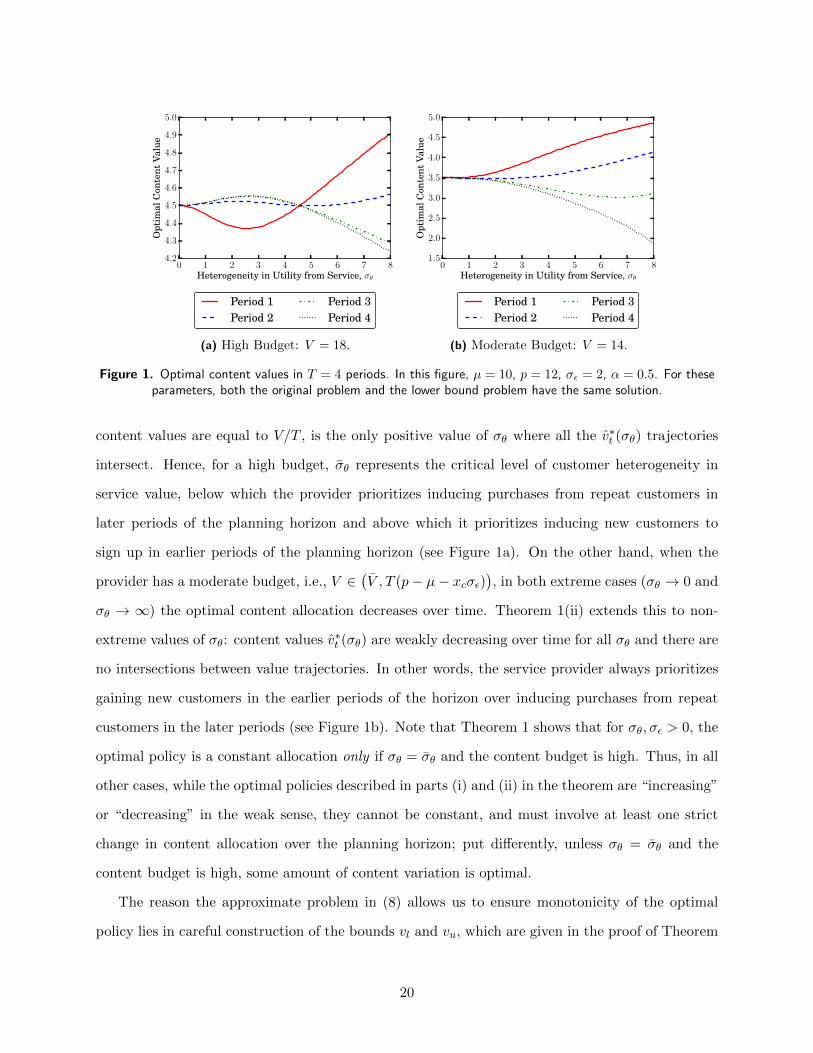
Figure 1. Optimal content values in T = 4 periods. In this figure, µ = 10, p = 12, σε = 2, α = 0.5. For theseparameters, both the original problem and the lower bound problem have the same solution.

content values are equal to V/T , is the only positive value of σθ where all the v∗t (σθ) trajectories

intersect. Hence, for a high budget, σθ represents the critical level of customer heterogeneity in

service value, below which the provider prioritizes inducing purchases from repeat customers in

later periods of the planning horizon and above which it prioritizes inducing new customers to

sign up in earlier periods of the planning horizon (see Figure 1a). On the other hand, when the

provider has a moderate budget, i.e., V ∈(V , T (p− µ− xcσε)

), in both extreme cases (σθ → 0 and

σθ → ∞) the optimal content allocation decreases over time. Theorem 1(ii) extends this to non-

extreme values of σθ: content values v∗t (σθ) are weakly decreasing over time for all σθ and there are

no intersections between value trajectories. In other words, the service provider always prioritizes

gaining new customers in the earlier periods of the horizon over inducing purchases from repeat

customers in the later periods (see Figure 1b). Note that Theorem 1 shows that for σθ, σε > 0, the

optimal policy is a constant allocation only if σθ = σθ and the content budget is high. Thus, in all

other cases, while the optimal policies described in parts (i) and (ii) in the theorem are “increasing”

or “decreasing” in the weak sense, they cannot be constant, and must involve at least one strict

change in content allocation over the planning horizon; put differently, unless σθ = σθ and the

content budget is high, some amount of content variation is optimal.

The reason the approximate problem in (8) allows us to ensure monotonicity of the optimal

policy lies in careful construction of the bounds vl and vu, which are given in the proof of Theorem

20

1. These bounds come from the analysis of a function, defined as R(v, σθ) in the proof, that

derives from comparing the demand loss associated with swapping the content allocated to any two

successive periods. We show in the proof that under the optimal content allocation, it must be

true that R (vt, σθ) ≤ R(vt+1, σθ) for all t. Furthermore, R(v, σθ) is quasi-convex in v, and is either

increasing or has a unique minimum for v ≥ 0, which we denote v(σθ). The bounds vl and vu are

designed to ensure that the allocation in every period is either below this minimum v (σθ) if the

content budget is “low” relative to the problem parameters, or above the minimum v(σθ) if there

is sufficient content budget to achieve this. Because R (vt, σθ) is increasing in t under the optimal

policy and monotonic in vt when vl ≤ vt ≤ vu, this means the optimal vt’s are monotonic in t as

well, either increasing or decreasing over time depending on whether they have been restricted to

lie on the increasing or decreasing portion of R(v, σθ). Importantly, vl and vu are functions of the

problem parameters, including σθ. Depending on the precise σθ value either vl = 0 or vu = V , while

the other bound is v (σθ) (or possibly V , if this is smaller), so the restriction that vl ≤ vt ≤ vu for

all t is relatively weak, leading to minimal loss in the objective function value in the instances where

the approximate solutions does not coincide with the optimal solution of the original problem, as

described further below.

Because Theorem 1 presents the optimal policy for an approximation to the original problem

in (5), we next discuss the impact of using such an approximation on firm decisions—i.e., the

optimal content allocation—as well as the objective function value. To that end, we conducted an

extensive numerical study involving close to 4.2 million combinations of the parameters α, p, µ,

σε, σθ, V , and T , calculating the optimal solution to the original problem (5), the optimal solution

to the lower bound problem (8), and the objective function value under a constant allocation

for each instance. The parameters considered in the numerical study consisted of the following:

α ∈ {0, 0.25, 0.50, 0.75}; T ∈ {2, 3, 4, 5}; p, µ ∈ {6, 8, 10, 12, 14}; ten equally spaced values of σε in

the interval[⌈∣∣∣p−µ−xc ∣∣∣⌉+ 1,max

{2⌈∣∣∣p−µ−xc ∣∣∣⌉+ 1, 10

}], ensuring instances that correspond to both the

moderate- and high-budget regions; V = Vmin+(z/10)(Vcrit−Vmin), where z = odd numbers between

3 and 23, Vmin = max{0, T (p−µ)}, and Vcrit = T (p−µ− xcσε), discarding any values that do not

satisfy V > V ; and, a hundred equally-spaced values of σθ in the interval [0,max {12, d1.5σθe}].

The average gap between the objective function under the optimal and approximate solutions

was 0.000036%, while the maximum gap between the two was 0.092%, suggesting that the lower

21

bound approximation is tight. Moreover, out of all the instances considered in this numerical study,

the solution to the original problem satisfied the constraints vl ≤ vt ≤ vu (and therefore coincided

with the solution to the lower bound problem) in 85.23% of the cases, and even in the instances in

which the constraints were not met, the optimal solution was also monotone. Thus, our numerical

study suggests that the allocation policy in Theorem 1 is optimal in a significant majority of cases

and, in the cases where it is not, introducing the constraints vl ≤ vt ≤ vu results in negligible loss

in the objective function value. Moreover, as shown in Propositions 3 and 4, the optimal solution

to the original problem is always monotone in the extreme cases when σθ → 0 and σθ →∞, and it

is constant for σθ = σθ.

Thus far, we have studied how the provider’s optimal allocation depends on customer het-

erogeneity in service utility, σθ. Theorem 2 describes the impact of a different type of customer

heterogeneity on the provider’s optimal policy: heterogeneity in customer value for content, σε. As

with σθ, it is not possible to characterize the monotonicity of the optimal policy as a function of

σε for the original problem in (5). Hence, we again consider the lower bound problem in (8). In

Theorem 2, we denote the optimal solution of (8) as v∗t (σε), making now explicit the dependence

on σε.

Theorem 2. For any σθ, σε > 0 and V ≥ 2T (p − µ), there exists a unique threshold σε such

that v∗t (σε), the optimal content allocation policy for the approximate problem in (8) with the lower

and upper bounds identified in Theorem 1, is increasing over time when σε < σε, constant only if

σε = σε, and decreasing over time when σε > σε.

Figure 2 shows the optimal content allocation policy as a function of σε for T = 4. Similar to the

behavior described in Propositions 3 and 4, we find that content values should always increase over

time when σε → 0 and always decrease over time when σε →∞. Therefore, at the two extremes the

optimal allocation policy is always monotonic even without the additional constraints. Additionally,

there exists a unique σε where all content value trajectories intersect. Theorem 2 shows that the

solution to the approximate problem is such that the content allocation policy is increasing over

time for σε < σε and decreasing over time for σε > σε; in addition, a constant allocation is only

optimal when σε = σε, meaning content variation is optimal in all other instances where σε > 0.

Note that Theorem 2 includes a slightly stronger condition (that V ≥ 2T (p−µ) rather than V > V )

22

1 2 3 4 5 6 7

Heterogeneity in Utility from Content, σε

2

3

4

5

6

7

Opt

imal

Con

tent

Valu

ePeriod 1Period 2

Period 3Period 4

Figure 2. Change in optimal content value with σε. In this figure, σθ = 8, while the other parameters are as inFigure 1a. For these parameters, both the original problem and the lower bound problem have the same solution.

on the content budget; this is necessary to determine the optimal allocation when σε → 0.

Monotonicity is guaranteed in the optimal policy because of an argument identical to that

provided after Theorem 1 (since Theorem 2 uses the same approximation as Theorem 1). In

addition, the numerical study discussed earlier includes ten equally spaced values of σε in the interval[⌈∣∣∣p−µ−xc ∣∣∣⌉+ 1,max{

2⌈∣∣∣p−µ−xc ∣∣∣⌉+ 1, 10

}]for each of approximately 0.42 million unique combinations

of the other parameters, and thus serves as a validation of the insights in Theorem 2 as well as

those in Theorem 1; this confirms that the lower bound approximation (8) performs very well as σε

varies, and yields the unconstrained optimal solution in a significant majority (85.23%) of cases.

To summarize, the analysis in this section illustrates precisely how a service provider can use

content variation to increase demand and, moreover, the significant impact that new customers

and their ability to learn about service utility have on the provider’s optimal content allocation

policy: any deviation from a constant allocation is driven by the presence of these new (as opposed

to repeat) customers, and the provider changes its content value over time to balance the rate at

which new customers first try the service and the rate at which they continue their service. The

insights from these results are summarized in Figure 3. Observe that whenever customers are very

heterogeneous in either content utility or service utility, the provider should use a decreasing content

allocation policy, i.e., by beginning with high content value in period 1 and decreasing it thereafter.

Put differently, the provider should focus on acquiring new customers early in the planning horizon

with high value content, but should decrease the value of that content afterwards, relying instead

23

0 5 10 15 20 25 30 35 40

Heterogeneity in Service Utility, σθ

0.0

0.5

1.0

1.5

2.0

2.5

3.0

Het

erog

enei

tyin

Con

tent

Uti

lity,σε

Content Value

Increases Over Time

Content Value

Decreases Over Time

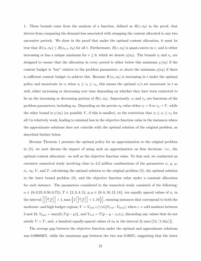
Figure 3. Service provider’s optimal content allocation policy. All parameter values are the same as in Figure 1a.

on customers with particularly high realizations of service or content value to continue using the

service.

On the other hand, when overall heterogeneity is low (i.e., if both σθ and σε are small), the

provider should follow an increasing content allocation policy, i.e., beginning with a relatively low

content value in period 1 and increasing it thereafter. In other words, it should focus on retaining

current customers by offering progressively better content over time. In this case, customer hetero-

geneity (in either service or content utility) is too small to drive significant repeat purchases, so the

provider must induce repeat purchases by offering more valuable content in each period, encourag-

ing those customers who realize low values of θi to become repeat purchasers. The critical threshold

that governs the transition between these two strategies (represented by the curve in Figure 3) is

characterized by σε and σθ and represents the levels of heterogeneity at which the provider offers

equal value in all periods. Accordingly, while intuition might suggest that service providers should

offer constant value content through a planning horizon, these results show that constant value

is only optimal under specific market conditions; in most cases, the optimal content allocation is

monotonically increasing (if customer heterogeneity is low) or decreasing (if heterogeneity is high)

over time.

5 Drivers of Content Variation

Thus far, we have discussed how the service provider should vary its content by analyzing the

optimal allocation policy within a planning horizon of T ≥ 2 periods. In doing so, we demonstrated

that intertemporal content variation—rather than a constant allocation—was, in general, optimal

24

for the firm. However, a natural question for firms facing this problem is: when is it most important

to pursue content variation? In this section, we answer this question by exploring when the optimal

allocation most significantly deviates from a constant allocation as a function of the composition of

the customer population (specifically, the fraction of repeat customers α) and the available content

budget V . For tractability purposes, in this section we restrict attention to a planning horizon

consisting of two periods (i.e., T = 2). We note that for the case of T = 2, the monotonicity results

derived in Theorems 1 and 2 hold for the optimal solution to the original problem in (5).

5.1 Composition of the Customer Population

The following result describes how the provider’s optimal allocation policy for a two-period planning

horizon—and the resulting optimal demand—change with the fraction of repeat customers, α.

Proposition 5. When T = 2, as α increases, the difference between the optimal values in the two

periods, |v∗1(α)− v∗2(α)|, as well as the optimal demand, weakly decrease.

A new customer i initially does not know his service utility θi and purchases in period t ∈ {1, 2}

if the expected service utility satisfies E[uit|εit] = µ + vt + εit − p ≥ 0. Therefore, it is possible

that he signs up, only to experience a negative net utility, i.e., θi + vt + εit − p < 0. On the other

hand, a repeat customer knows his service utility before making a purchasing decision, and will

never purchase if his net utility is negative. As α increases, the fraction of new customers decreases

and, from the perspective of the service provider, the likelihood of “erroneous” purchases from new

customers—customers paying the price p only to realize a negative net utility in a period—declines.

Consequently, the provider’s demand decreases with α.

At the same time, as α increases, the provider divides its budget more evenly over time, for two

reasons. First, as it follows from our discussion in §4, the principal trade-off that the provider faces

while choosing its optimal content allocation policy in a two-period horizon is whether to induce

new customers to sign up in period 1 by setting a high v1 or to persuade those new customers who

signed up in period 1 to continue their service in period 2 by setting a high v2. As α increases,

the importance of this trade-off decreases since there are fewer new customers in the market.

Second, the provider’s optimal allocation policy when catering to repeat customers is to divide the

budget equally in the two periods because of the “S” shape of the demand function (as discussed

25

in Proposition 2). Hence, when there are fewer new (and more repeat) customers at the beginning

of a planning horizon, the provider employs a more even content allocation policy; in the extreme

case when α = 1, content value is constant over time.

The above proposition sheds some light on how the provider’s content allocation should change

during the life-cycle of the firm. For a new firm, almost all customers will be new and unaware of

their service utility θi. Even if some of them sign up, learn this utility, and become repeat customers,

the firm would be able to rapidly grow its customer base by expanding into new markets and adding

new customers who have not used the service before. Hence, we expect that α should generally be

low for a young firm; consequently, the provider would find it optimal to significantly vary content

value during the planning horizon.

While keeping α low might be possible for a young firm that is expanding to new markets and

customer populations at a rapid pace, it becomes progressively more difficult over time as the firm

matures and the market saturates. Hence, with time, most potential customers will try the service

at least once and learn their valuations, becoming “repeat” customers (i.e., ones that know θi), and

the firm will not be able to replenish the depleting pool of new customers through expansion. As a

result, the fraction of repeat customers in the market is likely to increase as the firm matures, and

the provider will find it optimal to distribute its budget more evenly over time (i.e., v∗1 and v∗2 both

move towards V/2). Although content variation will still be optimal, the difference between the

two values will diminish over time until, finally, essentially all customers will have tried the service

at least once and will become repeat customers (i.e., α = 1); once this occurs, the provider will

find it optimal to set a constant content value in all periods. Consequently, Proposition 5 suggests

that content variation is most critical for young firms with many potential new customers; as firms

mature, content variation should decrease and the optimal policy should move towards a constant

allocation over time.

5.2 Content Budget

Next, we explore how the amount of variation in the optimal allocation policy depends on the

provider’s budget, V . In what follows, we make explicit the dependence of the optimal content

allocation policy on the budget by denoting it by v∗1(V ) and v∗2(V ).

26

Proposition 6. (i) For any p > µ, limV↘V v∗1(V ) ∈

[min

{V, V

[12 + σε

2(p−µ)

]}, V].

(ii) When V →∞, a constant allocation, v∗1(V ) = v∗2(V ) = V/2, is always an optimal allocation.

Proposition 6 part (i) demonstrates that when V is closer to its lower bound, i.e., V ↘ V ,

the provider will find it optimal to allocate most of its budget to the first period. In a two-period

horizon, if p > µ, the lower bound is V = 2(p−µ). (If p ≤ µ, then V = 0, in which case there is no

content to allocate in this boundary scenario. We therefore only consider the case with p > µ in

this part of the proposition.) From Theorem 1(ii), we know that for any V ∈ (V , 2(p− µ− xcσε)),

the provider should allocate at least half of its budget to period 1. Proposition 6(i), states that

in the extreme case when V ↘ V , the optimal fraction is, in fact, at least min{

1, 12 + σε

2(p−µ)

}.

For sufficiently large σε (specifically, σε > p− µ), this implies that the optimal allocation is one of

extreme content variation, with all of the budget allocated to period 1. In other words, when the

budget is limited (i.e., as the budget approaches the lower bound of the “moderate” region), the

provider finds it more important to engage in content variation and, as a result, the optimal policy

deviates most significantly from a constant allocation. This is intuitive: because of increasing

returns to scale for the normal distribution function at low arguments, the provider’s demand

function is higher if it allocates more of its budget to a single period instead of allocating the same

budget to two different periods. The condition that V ↘ V essentially ensures that the provider’s

objective function is in this “increasing returns to scale” region for any content allocation, hence

the optimal allocation is one of maximal content variation.

In contrast, part (ii) of Proposition 6 shows that when the budget is unlimited, a constant

allocation is always optimal; this is because, with a very high budget, the provider finds itself in

the region of decreasing returns to scale for the normal distribution function at high arguments.

However, we note that in this case, there may be many allocations that result in identical demand

(equal to the maximum possible demand), i.e., the optimal allocation may not be unique. This

result illustrates that a constant allocation is sufficient for optimality when the budget is very large

or, in other words, that content variation is less critical.

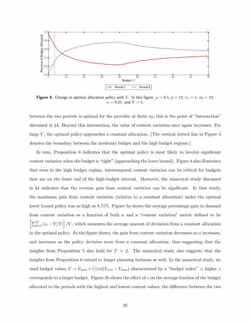
Filling in between the two extreme cases in the proposition, Figure 4 shows that as the budget

increases from its lower limit, the provider divides the budget more evenly and content variation

becomes less extreme. Furthermore, there exists a value of the budget such that an equal allocation

27

5 10 15 20 25 30 35 40 45 50

Budget, V

0.0

0.2

0.4

0.6

0.8

1.0

Fra

ctio

nof

Bud

get

Allo

cate

d

Period 1 Period 2

Figure 4. Change in optimal allocation policy with V . In this figure, µ = 9.5, p = 12, σε = 1, σθ = 10,α = 0.25, and V = 5.

between the two periods is optimal for the provider at finite σθ; this is the point of “intersection”

discussed in §4. Beyond this intersection, the value of content variation once again increases. For

large V , the optimal policy approaches a constant allocation. (The vertical dotted line in Figure 4

denotes the boundary between the moderate budget and the high budget regions.)

In sum, Proposition 6 indicates that the optimal policy is most likely to involve significant

content variation when the budget is “tight” (approaching the lower bound). Figure 4 also illustrates

that even in the high budget regime, intertemporal content variation can be critical for budgets

that are on the lower end of the high-budget interval. Moreover, the numerical study discussed

in §4 indicates that the revenue gain from content variation can be significant. In that study,

the maximum gain from content variation (relative to a constant allocation) under the optimal

lower bound policy was as high as 8.71%. Figure 5a shows the average percentage gain in demand

from content variation as a function of both α and a “content variation” metric defined to be[∑Tt=1 |vt − V/T |

]/V , which measures the average amount of deviation from a constant allocation

in the optimal policy. As the figure shows, the gain from content variation decreases as α increases,

and increases as the policy deviates more from a constant allocation, thus suggesting that the

insights from Proposition 5 also hold for T > 2. The numerical study also suggests that the

insights from Proposition 6 extend to longer planning horizons as well. In the numerical study, we

used budget values V = Vmin + (z/10)(Vcrit − Vmin) characterized by a “budget index” z; higher z

corresponds to a larger budget. Figure 5b shows the effect of z on the average fraction of the budget

allocated to the periods with the highest and lowest content values; the difference between the two

28

0.0 0.3 0.6 0.9 1.2 1.5

Content Variation Exceeds

0.0

0.5

1.0

1.5

2.0

2.5

3.0

3.5

4.0

Ave

rage

%D

eman

dG

ain

α = 0.00

α = 0.25

α = 0.50

α = 0.75

(a) Average % Demand Gain for VariousThreshold Values of Content Variation.

3 7 11 15 19 23

Budget Index, z

0.20

0.25

0.30

0.35

0.40

0.45

0.50

0.55

Ave

rage

Fra

ctio

nof

Bud

get

maxt {vt} /V mint {vt} /V

(b) Average Fraction of Budget Allocated to thePeriods of the Planning Horizon with the Highest and

the Lowest Content Values for Different Budget Indices.

Figure 5. Results from the Numerical Study.

fractions serves as another measure of the degree of content variation in the optimal policy. As the

figure shows, content variation is greatest when the budget is tight, i.e., z is small, and exhibits

behavior consistent with Figure 4 and Proposition 6 as z increases. The study does not include

large enough values of z to show limiting behavior; however, regardless of the horizon length, a

constant allocation of an infinite budget will result in infinite content value in each period, and

will constitute an optimal allocation. Hence, content variation will not be critical as V →∞ even

when T > 2.

6 Conclusion

Services where providers have the ability to vary the content over time are becoming more prevalent.

While many traditional business models have the ability to vary prices over time to influence

customer purchasing decisions and maximize revenue, these new services typically operate with a

constant price. This raises the question of how a service provider can use intertemporal content

variation—as opposed to dynamic pricing—to maximize demand and revenue. What makes this

problem challenging is that providers typically have limited resources and hence face a constraint on

the total budget for content that they may employ within a planning horizon. Hence, the provider

29

is forced to trade off the benefit of offering highly valued content in one period (raising demand in

that period) with the cost of offering less valuable content in another period (lowering demand in

that period).

We find that the optimal content allocation policy is not, in general, to offer content of equal

value over time. Instead, it depends critically on the level of heterogeneity in both components of

utility in the customer population. Using a lower bound approximation to derive an optimal policy

to the general allocation problem, we show that a simple policy of monotonically increasing the level

of content value over time when heterogeneity is low, and monotonically decreasing content value

over time when heterogeneity is high is either optimal or nearly so in the vast majority of cases.

When customer heterogeneity is low, the provider cannot rely on heterogeneity to encourage repeat

purchases (i.e., because many customers have especially high content or service value), and so the

provider itself must encourage such purchases by offering increasingly better content over time. In

contrast, when heterogeneity is high, customer heterogeneity will spur most repeat purchases, so

the provider’s goal should be to get as many customers as possible to experience service for the

first time early in a planning horizon, maximizing the number of opportunities for repeat purchases

based on heterogeneous realizations of content or service utility; this results in a monotonically

decreasing content allocation policy.

We also analyzed how the amount of content variation in the provider’s optimal allocation policy

depends on the market composition and the content budget. We found that a provider catering to

a market with a large fraction of new customers who have never used the service before (and hence

do not know their utilities from service) should offer a higher degree of content variation; this is

likely to be particularly applicable for newer firms rapidly expanding into new markets and facing

many new potential customers. However, as the service matures and more customers learn their

utilities, the provider should divide the budget more evenly, and in the extreme case of a market

with no new customers, offer content of equal value throughout the horizon.

In addition, we showed that a service with a more limited budget should vary content more

over time. On the other hand, when the budget is extremely large, a constant allocation is optimal.

Beyond demonstrating how the budget constraint impacts the optimal policy, this reinforces our

findings regarding the market composition: newer firms are both more likely to face a larger fraction

of “new” customers (low α) and a smaller budget (low V ) and, in both cases, content variation is

30

more critical for the firm.

While we have assumed that the firm maximizes revenue (or demand) subject to a fixed budget

constraint, as noted in §3, an extended version of our model might endogenize the budget itself and

maximize revenue net of the budget, i.e., solving maxV≥0 (pD∗(V )− CV ), where C > 0 represents

the cost of one unit of budget and D∗(V ) is the optimal demand for a fixed budget that we have

analyzed in this paper. We have studied such an extension for the special case of T = 2 periods,

and have found that, depending on the parameter C, the optimal budget level may lie in either the

moderate or high regions that we identify in §4; hence, the insights and different cases that we have

identified with a fixed budget (i.e., that the optimal allocation is monotone and may be increasing

or decreasing over time) persist even under an endogenously set budget.

We note that our model abstracts from several issues that firms may face when determining

their content allocation policy, many of which are context specific. For example, video streaming

platforms may be constrained in their allocation decisions by licensing agreements, genre consider-

ations (e.g., some genres of content are more important to release in certain months), or seasonality

of customer viewing habits. Subscription box services may likewise be constrained by availability

of certain items (e.g., for meal kit services, certain fruits or vegetables may only be available during

specific times of the year). For some firms, content may be discrete rather than continuous as we

have assumed. While we have not included such details in our model, our goal has been to analyze

a generic content allocation problem that is applicable to a variety of different settings to under-

stand the key aspects of the interplay between content and demand, and we have included the most

critical features of that problem—allocating a fixed budget to maximize revenue or demand—in as

parsimonious a model as possible. We acknowledge that models incorporating additional details

may yield further interesting insights about content allocation in specific contexts; our hope is that

future work can address exactly these issues and advance our understanding of how best to allocate

content over time.

Taken in sum, our results show how new business models—such as video streaming services

and curated subscription boxes—can lead to new ways for firms to influence customer purchasing

decisions, in our case maximizing revenue by varying the content of the service over time, rather than

the price of that content. As such business models continue to grow in popularity, understanding

how to use all the levers available to firms to maximize demand will be of increasing importance.

31

Our model thus provides a first step in this direction by studying optimal intertemporal content

variation under customer learning.

References

Adelman, Daniel, & Mersereau, Adam J. 2013. Dynamic Capacity Allocation to Customers Who Remember

Past Service. Management Science, 59(3), 592–612.

Aflaki, Sam, & Popescu, Ioana. 2014. Managing Retention in Service Relationships. Management Science,

60(2), 415–433.

Baucells, Manel, & Sarin, Rakesh K. 2007. Satiation in Discounted Utility. Operations Research, 55(1),

170–181.

Baucells, Manel, & Sarin, Rakesh K. 2010. Predicting Utility Under Satiation and Habit Formation. Man-

agement Science, 56(2), 286–301.

Bernstein, Fernando, & Martınez-de Albeniz, Victor. 2017. Dynamic Product Rotation in the Presence of

Strategic Customers. Management Science, 63(7), 2092–2107.

Caro, Felipe, & Martınez-de Albeniz, Victor. 2020. Managing Online Content to Build a Follower Base:

Model and Applications. INFORMS Journal on Optimization, 2(1), 57–77.

Caro, Felipe, Martınez-de Albeniz, Victor, & Rusmevichientong, Paat. 2014. The Assortment Packing

Problem: Multiperiod Assortment Planning for Short-Lived Products. Management Science, 60(11),

2701–2721.

Caulkins, Jonathan P., Feichtinger, Gustav, Haunschmied, Josef, & Tragler, Gernot. 2006. Quality Cycles

and the Strategic Manipulation of Value. Operations Research, 54(4), 666–677.

Das Gupta, Aparupa, Karmarkar, Uday S., & Roels, Guillaume. 2016. The Design of Experiential Services

with Acclimation and Memory Decay: Optimal Sequence and Duration. Management Science, 62(5),

1278–1296.

Desai, Preyas S. 2001. Quality segmentation in spatial markets: When does cannibalization affect product

line design? Marketing Science, 20(3), 265–283.

Digital Trends. 2020. What’s new on Netflix, and what’s leaving in June 2020.

Dixon, Michael, & Verma, Rohit. 2013. Sequence effects in service bundles: Implications for service design

and scheduling. Journal of Operations Management, 31(3), 138–152.

Dixon, Michael J., & Thompson, Gary M. 2016. Bundling and Scheduling Service Packages with Customer

Behavior: Model and Heuristic. Production and Operations Management, 25(1), 36–55.

Engadget. 2018. Apple Music makes it easier to see new albums that are on the way.

Feldman, Pnina, Papanastasiou, Yiangos, & Segev, Ella. 2019. Social Learning and the Design of New

Experience Goods. Management Science, 65(4), 1502–1519.

Ferreira, Kris Johnson, & Goh, Joel. 2020. Assortment Rotation and the Value of Concealment. Management

Science, Forthcoming.

Forbes. 2018. Exclusive: 60% Of U.S. Amazon Customers Will Not Renew Their Prime Membership, Poll

Reveals.

Forbes. 2019. Analysis: Here’s why Netflix won’t raise prices again in 2020.

32

Hall, Joseph, & Porteus, Evan. 2000. Customer Service Competition in Capacitated Systems. Manufacturing

& Service Operations Management, 2(2), 144–165.

Jerath, Kinshuk, Kim, Sang-Hyun, & Swinney, Robert. 2017. Product quality in a distribution channel with

inventory risk. Marketing Science, 36(5), 747–761.

Liu, Ben Shaw-Ching, Petruzzi, Nicholas C., & Sudharshan, D. 2007. A service effort allocation model for

assessing customer lifetime value in service marketing. Journal of Services Marketing, 21(1), 24–35.

Liu, Qian, & van Ryzin, Garrett. 2011. Strategic Capacity Rationing when Customers Learn. Manufacturing

& Service Operations Management, 13(1), 89–107.

Manjoo, Farhad. 2016. Why Media Titans Would Be Wise Not to Overlook Netflix. The New York Times,

Jan.

Mussa, Michael, & Rosen, Sherwin. 1978. Monopoly and product quality. Journal of Economic theory,

18(2), 301–317.

Popescu, Ioana, & Wu, Yaozhong. 2007. Dynamic Pricing Strategies with Reference Effects. Operations

Research, 55(3), 413–429.

Sundaram, Rangarajan K. 1996. A First Course in Optimization Theory. Cambridge University Press.

Talluri, Kalyan T, & Van Ryzin, Garrett J. 2006. The theory and practice of revenue management. Vol. 68.

Springer Science & Business Media.

Ulu, Canan, Honhon, Dorothee, & Alptekinoglu, Aydın. 2012. Learning Consumer Tastes Through Dynamic

Assortments. Operations Research, 60(4), 833–849.

USA Today. 2019. Netflix price increases could cause some subscribers to downgrade, cancel streaming

service.

Verhoef, Peter C., Antonides, Gerrit, & de Hoog, Arnoud N. 2004. Service Encounters as a Sequence of

Events: The Importance of Peak Experiences. Journal of Service Research, 7(1), 53–64.

Wathieu, Luc. 1997. Habits and the Anomalies in Intertemporal Choice. Management Science, 43(11),

1552–1563.

33

Online Supplement to “Intertemporal Content Variation with

Customer Learning”

A Appendix: Proof of Results

To simplify the notation, let λ(x) = φ(x)Φ(x)

denote the failure rate function and g(x) = xλ(x)

denote the generalized failure rate function for the standard normal distribution. For the standardnormal, the generalized failure rate function g(x) decreases in (−∞, xc] and increases in [xc,+∞),where xc ≈ −0.84 is the unique solution to Φ(x) − x2Φ(x) + xφ(x) = 0. The proof of the resultsdiscussed in the main text are presented below.

Proof of Proposition 1: We prove (3) by induction. Observe that a repeat customer i who hasused the service in a previous planning horizon and already knows θi before period 1 will use theservice in period t ∈ {1, 2, ..., T} only if uit = θi+vt+εit−p ≥ 0. Since θi+εit ∼ N(µ, σ2

ε +σ2θ), from

the provider’s perspective before period 1, customer i will use the service in period t with probability

Φ

(p−µ−vt√σ2ε+σ2

θ

). On the other hand, an initially (i.e., before period 1) new customer j will sign up for

the service in period t if E[ujt] = µ+ vt + εjt − p ≥ 0, i.e., if εjt ≥ p− µ− vt. Since εjt ∼ N(0, σ2ε )

from the provider’s perspective before period 1, customer j will sign up in period t with probability

Φ(p−µ−vtσε

). Since the market consists of an α fraction of repeat customers and a 1−α fraction of

new customers, total demand when T = 1 is D|T=1 = αΦ

(p−µ−v1√σ2ε+σ2

θ

)+ (1− α)Φ

(p−µ−v1

σε

). Thus,

(3) holds when T = 1.Suppose that (3) also holds for T − 1 for any T > 2. Hence, total demand in periods 1 to T − 1

is D|T−1 =

= α

T−1∑t=1

Φ

(p− µ− vt√σ2ε + σ2

θ

)+ (1− α)

[1−

T−1∏t=1

Φ

(p− µ− vt

σε

)+

T−1∑t=2

Φ

(p− µ− vt√σ2ε + σ2

θ

){1−

t−1∏i=1

Φ

(p− µ− vi

σε

)}].

Demand in period T from customers who are new at the beginning of the horizon is given by

DNT = Φ

p− µ− vT√σ2ε + σ2

θ

[1−T−1∏i=1

Φ

(p− µ− vi

σε

)]+Φ

(p− µ− vT

σε

) T−1∏i=1

Φ

(p− µ− vi

σε

). (A.1)

The first term is the probability that a new customer used the service at least once in the firstT − 1 periods and is using it again in period T , while the second term is the probability that a newcustomer who has never used the service before is using it for the first time in period T . Hence, the

total demand in period T is DT = αΦ

(p−µ−vT√σ2ε+σ2

θ

)+ (1− α)DN

T . Observe that D|T = D|T−1 +DT .

Hence, by induction, (3) holds for any T .

1

Proof of Proposition 2: When σθ = 0, the total demand in (3) reduces to

D = ΣTt=1Φ

(p− µ− vt

σε

).

We divide the proof into the following lemmas.

Lemma A.1. Assume σθ = 0. If µ + VT > p, then v∗t = V

T ∀ t ∈ {1, 2, ..., T} is a strict localmaximum to the provider’s problem.

Proof. The provider solves the constrained optimization problem: Maximize D subject to ΣTt=1vt =

V . Define the Lagrangian, L = D+λ(V −ΣTt=1vt), where the Lagrangian multiplier, λ ≥ 0. ∂L

∂vt= 0

implies φ(p−µ−vtσε

)= σελ for all t ∈ {1, ..., T}. Let x∗ ≥ 0 be such that φ(x∗) = σελ. Note that

there could be three possible cases.Case 1:

p−µ−v∗tσε

= −x∗ ≤ 0 for all t ∈ {1, ..., T}. This implies that the provider sets value

v∗t = p− µ+ x∗σε in all periods. From∑T

t=1 v∗t = V , x∗ =

µ+VT−p

σε. Hence, x∗ ≥ 0 is possible only

if µ + VT ≥ p. Therefore, v∗t = V

T and λ∗ = 1σεφ

(µ+V

T−p

σε

). To study the second order condition,

we follow Theorem 5.4 of Sundaram (1996), and define a set of vectors

Z =

{z ∈ RT

∣∣∣∣∣[∂

∂v1

(V −

T∑t=1

vt

), ...,

∂

∂vT

(V −

T∑t=1

vt

)]z = 0

}=

{z ∈ RT

∣∣∣∣∣T∑t=1

zt = 0

}.

Further observe that the second derivative, D2L(v∗, λ∗), is a diagonal matrix with elementsp−µ−v∗tσ3ε

φ(p−µ−v∗t

σε

)≤ 0 (since, v∗t = V

T ≥ p− µ). This is a local maximum because

z′D2L(v∗, λ∗)z =

T∑t=1

z2t

p− µ− v∗tσ3ε

φ

(p− µ− v∗t

σε

)≤ 0.

Case 2:p−µ−v∗t

σε= x∗ ≥ 0 for all t ∈ {1, ..., T}. Therefore, v∗t = p − µ − x∗σε in all periods.

From∑T

t=1 v∗t = V , x∗ = −µ+V

T−p

σε. Hence, x∗ ≥ 0 is possible only if µ + V

T ≤ p. Therefore,

v∗t = VT and λ∗ = 1

σεφ

(−µ+V

T−p

σε

). The second derivative test now results in z

′D2L(v∗, λ∗)z =∑Tt=1 z

2tp−µ−v∗tσ3ε

φ(p−µ−v∗t

σε

)≥ 0. Hence, this is a local minimum.

Case 3: Now suppose, without loss of generality,p−µ−v∗t

σε= x∗ for k ∈ {1, ..., T − 1} periods

andp−µ−v∗t

σε= −x∗ for the remaining T − k periods. In this case, x∗ =

µ+VT−p

(1−2 kT

)σεand λ∗ =

1σεφ

(µ+V

T−p

(1−2 kT

)σε

), which is neither a minimum nor a maximum. Indeed, consider zt = γ(> 0) for

one of the k periods withp−µ−v∗t

σε= x∗, zt = 0 for the other k − 1 periods with

p−µ−v∗tσε

= x∗

and zt = − γT−k for each of the T − k periods with

p−µ−v∗tσε

= −x∗. We have z′D2L(v∗, λ∗)z =

x∗φ(x∗)σ2ε

[γ2 − (T − k) γ2

(T−k)2

]≥ 0. Now consider z such that zt = γ(> 0) for one of the T−k periods

withp−µ−v∗t

σε= −x∗, zt = 0 for the remaining T − k − 1 periods with

p−µ−v∗tσε

= −x∗ and zt = −γk

2

for each of the k periods withp−µ−v∗t

σε= x∗. Then, z

′D2L(v∗, λ∗)z = x∗φ(x∗)σ2ε

[−γ2 + k γ

2

k2

]≤ 0.

Lemma A.2. When σθ = 0, there exists a threshold, V , such that v∗t = VT ∀ t ∈ {1, 2, ..., T} is

the unique global maximum for any V > V . The threshold V ∈ [T (p− µ), 2T (p− µ)) if p > µ;otherwise, V = 0.

Proof. Observe that we have ignored the constraints vt ≥ 0 ∀ t ∈ {1, ...T} in our analysis above.Now suppose we impose this constraint by making some of the vt to be zero. From Lemma A.1, itfollows that an allocation with v∗t = V

k for any k periods, where k ∈ {1, 2, ..., T − 1} and v∗t = 0 inthe remaining T −k periods is also a strict local maximum when µ+ V

T > p (since µ+ Vk > p). The

allocation, v∗t = VT ∀ t ∈ {1, 2, ..., T} is the unique global maximum if, for any k ∈ {1, 2, ..., T − 1}

kΦ

(p− µ− V

k

σε

)+ (T − k)Φ

(p− µσε

)< T Φ

(p− µ− V

T

σε

). (A.2)

Observe that as V increases, the right-hand side of (A.2) increases faster than the left-hand side forany k < T . Moreover, as V →∞, the inequality in (A.2) holds. Therefore, there exists a unique V

′

such that (A.2) holds for any V > V′

and v∗t = VT ∀ t ∈ {1, 2, ..., T} is the unique global maximum

for any V > max{V ′ , T (p− µ)} ≡ V .Further note that the left hand side of (A.2) satisfies

∂LHS

∂k≡ Φ

(p− µ− V

k

σε

)− Φ

(p− µσε

)− V

kσεφ

(p− µ− V

k

σε

)

and ∂2LHS∂k2

= V 2

k3σ2ε

p−µ−Vk

σεφ

(p−µ−V

kσε

)< 0 for any k < T . If p ≤ µ, ∂LHS∂k > 0 and the left-hand side

of (A.2) is strictly increasing in k; hence, (A.2) is true for any V > 0. If p > µ, a k∗ < T that satisfies∂LHS∂k |k∗ = 0, i.e., maximizes the left-hand side of (A.2), can only exist if V < 2k∗(p−µ). Therefore,

a sufficient condition for (A.2) to be true is V ≥ 2T (p− µ). Hence, V ∈ [T (p− µ), 2T (p− µ)).

Proof of Proposition 3 : We provide a proof by contradiction. Suppose the optimal solutionallocates vH in period k and vL(< vH) in period k + 1 for any k ∈ {1, 2, ..., T − 1} and achievestotal demand DHL. Consider an allocation where we switch the content values in periods k andk + 1 (i.e., vk = vL and vk+1 = vH) while keeping all other periods unchanged. Let the new totaldemand be DLH . From (3), note that DLH −DHL =

= (1− α)

k−1∏i=1

Φ

(p− µ− vi

σε

)Φ

p− µ− vH√σ2ε + σ2

θ

Φ

(p− µ− vL

σε

)− Φ

p− µ− vL√σ2ε + σ2

θ

Φ

(p− µ− vH

σε

) . (A.3)

Observe that if ∂∂σ

Φ(p−µ−vH

σ

)Φ(p−µ−vL

σ

)∣∣∣∣∣σ=σε

> 0, then DLH − DHL > 0 when σθ is infinitesimally small.

Now,

∂

∂σ

Φ(p−µ−vH

σ

)Φ(p−µ−vL

σ

) ∣∣∣∣∣σ=σε

=1

σε

Φ(p−µ−vH

σ

)Φ(p−µ−vL

σ

) [g(p− µ− vHσε

)− g

(p− µ− vL

σε

)].

3

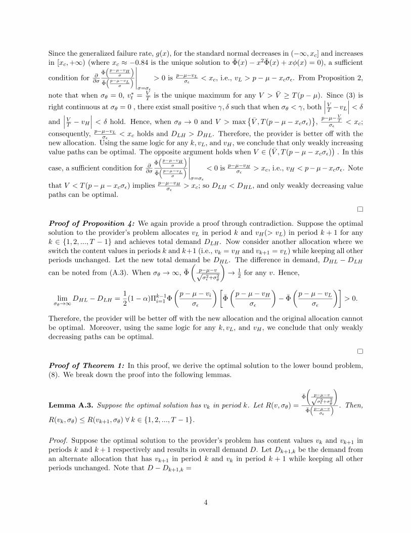
Since the generalized failure rate, g(x), for the standard normal decreases in (−∞, xc] and increasesin [xc,+∞) (where xc ≈ −0.84 is the unique solution to Φ(x) − x2Φ(x) + xφ(x) = 0), a sufficient

condition for ∂∂σ

Φ(p−µ−vH

σ

)Φ(p−µ−vL

σ

)∣∣∣∣∣σ=σε

> 0 is p−µ−vLσε

< xc, i.e., vL > p − µ − xcσε. From Proposition 2,

note that when σθ = 0, v∗t = VT is the unique maximum for any V > V ≥ T (p − µ). Since (3) is

right continuous at σθ = 0 , there exist small positive γ, δ such that when σθ < γ, both∣∣∣VT −vL∣∣∣ < δ

and∣∣∣VT − vH ∣∣∣ < δ hold. Hence, when σθ → 0 and V > max

{V , T (p− µ− xcσε)

},p−µ−V

Tσε

< xc;

consequently, p−µ−vLσε

< xc holds and DLH > DHL. Therefore, the provider is better off with thenew allocation. Using the same logic for any k, vL, and vH , we conclude that only weakly increasingvalue paths can be optimal. The opposite argument holds when V ∈

(V , T (p− µ− xcσε)

). In this

case, a sufficient condition for ∂∂σ

Φ(p−µ−vH

σ

)Φ(p−µ−vL

σ

)∣∣∣∣∣σ=σε

< 0 is p−µ−vHσε

> xc, i.e., vH < p−µ−xcσε. Note

that V < T (p− µ− xcσε) implies p−µ−vHσε

> xc; so DLH < DHL, and only weakly decreasing valuepaths can be optimal.

Proof of Proposition 4: We again provide a proof through contradiction. Suppose the optimalsolution to the provider’s problem allocates vL in period k and vH(> vL) in period k + 1 for anyk ∈ {1, 2, ..., T − 1} and achieves total demand DLH . Now consider another allocation where weswitch the content values in periods k and k+1 (i.e., vk = vH and vk+1 = vL) while keeping all otherperiods unchanged. Let the new total demand be DHL. The difference in demand, DHL − DLH

can be noted from (A.3). When σθ →∞, Φ

(p−µ−v√σ2ε+σ2

θ

)→ 1

2 for any v. Hence,

limσθ→∞

DHL −DLH =1

2(1− α)Πk−1

i=1 Φ

(p− µ− vi

σε

)[Φ

(p− µ− vH

σε

)− Φ

(p− µ− vL

σε

)]> 0.

Therefore, the provider will be better off with the new allocation and the original allocation cannotbe optimal. Moreover, using the same logic for any k, vL, and vH , we conclude that only weaklydecreasing paths can be optimal.

Proof of Theorem 1: In this proof, we derive the optimal solution to the lower bound problem,(8). We break down the proof into the following lemmas.

Lemma A.3. Suppose the optimal solution has vk in period k. Let R(v, σθ) =Φ

(p−µ−v√σ2ε+σ

2θ

)Φ(p−µ−vσε

) . Then,

R(vk, σθ) ≤ R(vk+1, σθ) ∀ k ∈ {1, 2, ..., T − 1}.

Proof. Suppose the optimal solution to the provider’s problem has content values vk and vk+1 inperiods k and k+ 1 respectively and results in overall demand D. Let Dk+1,k be the demand froman alternate allocation that has vk+1 in period k and vk in period k + 1 while keeping all otherperiods unchanged. Note that D −Dk+1,k =

4

= (1− α)

k−1∏i=1

Φ

(p− µ− vi

σε

)[Φ

(p− µ− vk+1√

σ2ε + σ2

θ

)Φ

(p− µ− vk

σε

)− Φ

(p− µ− vk√σ2ε + σ2

θ

)Φ

(p− µ− vk+1

σε

)].

Since, the allocation with vk in period k and vk+1 in period k+ 1 is optimal, D ≥ Dk+1,k whichcan be the case only if R(vk, σθ) ≤ R(vk+1, σθ).

Lemma A.4. (i) For a fixed σθ, R(v, σθ) is quasiconvex in v. When p−µ−xcσε ≥ 0, R(v, σθ) has aunique minimum, v(σθ), that satisfies limσθ→0 v(σθ) = p−µ−xcσε. When p−µ−xcσε < 0, a unique

minimum, v(σθ), only exists when σθ is sufficiently large and satisfies g

(p−µ√σ2ε+σ2

θ

)≥ g

(p−µσε

);

otherwise, R(v, σθ) is strictly increasing in v. Whenever the minimum, v(σθ), exists, it is strictlyincreasing with σθ.(ii) There always exists a unique σθ > 0 satisfying v(σθ) = V/T for any V > T (p− µ− xcσε),while such a σθ > 0 cannot exist for any V < T (p− µ− xcσε).

Proof. (i) Note again that the standard normal generalized failure rate function, g(x), decreases in(−∞, xc] and increases in [xc,+∞). Now,

∂

∂vR(v, σθ) = R(v, σθ)

1√σ2ε + σ2

θ

λ

p− µ− v√σ2ε + σ2

θ

− 1

σελ

(p− µ− v

σε

)=

R(v, σθ)

p− µ− v

g p− µ− v√

σ2ε + σ2

θ

− g(p− µ− vσε

) (A.4)

First suppose p−µ−xcσε ≥ 0. Consider any v ≤ p−µ−xcσε. From (A.4), observe that for this range

of v, p−µ−vσε≥ xc; hence, ∂

∂vR(v, σθ) < 0. Next consider any v ≥ p−µ−xc√σ2ε + σ2

θ . In this range of

v, p−µ−v√σ2ε+σ2

θ

≤ xc; hence, ∂∂vR(v, σθ) > 0. Therefore, by the continuity of ∂

∂vR(v, σθ), there must exist

at least one root of the function in the interval(p− µ− xcσε, p− µ− xc

√σ2ε + σ2

θ

). Let vo be one

such root of ∂∂vR(v, σθ). Since vo ∈

(p− µ− xcσε, p− µ− xc

√σ2ε + σ2

θ

), it follows that p−µ−vo

σε<

xc <p−µ−vo√σ2ε+σ2

θ

< 0 and g(p−µ−vo

σε

)= g

(p−µ−vo√σ2ε+σ2

θ

). Now pick a v ∈

(vo, p− µ− xc

√σ2ε + σ2

θ

). For

any such v, xc <p−µ−v√σ2ε+σ2

θ

< p−µ−vo√σ2ε+σ2

θ

< 0; hence, g

(p−µ−v√σ2ε+σ2

θ

)< g

(p−µ−vo√σ2ε+σ2

θ

)must be true. On

the other hand, p−µ−vσε

< p−µ−voσε

< xc must result in g(p−µ−vσε

)> g

(p−µ−vo

σε

)= g

(p−µ−vo√σ2ε+σ2

θ

)>

g

(p−µ−v√σ2ε+σ2

θ

). Therefore, g

(p−µ−vσε

)cannot be equal to g

(p−µ−v√σ2ε+σ2

θ

)and v cannot be another root

of the function ∂∂vR(v, σθ). Using a similar argument, we can show that no other root of ∂

∂vR(v, σθ)

can exist in the interval v ∈ (p− µ− xcσε, vo). Therefore, for a fixed σθ,∂∂vR(v, σθ) has a unique

root, which we denote by v(σθ). Moreover, R(v, σθ) is quasiconvex with a unique minimum atv(σθ). Finally observe that as σθ → 0, limσθ→0 v(σθ) = p− µ− xcσε.

5

To see how the unique minimum v(σθ) changes with σθ, we differentiate both sides of the

equality g(p−µ−v(σθ)

σε

)= g

(p−µ−v(σθ)√

σ2ε+σ2

θ

)with respect to σθ to obtain

dv(σθ)

dσθ=

σεσθσ2ε+σ2

θ

p−µ−v(σθ)√σ2ε+σ2

θ

∂∂vg

(p−µ−v√σ2ε+σ2

θ

) ∣∣∣∣v=v(σθ)

∂∂vg

(p−µ−vσε

) ∣∣∣∣v=v(σθ)

− σε√σ2ε+σ2

θ

∂∂vg

(p−µ−v√σ2ε+σ2

θ

) ∣∣∣∣v=v(σθ)

.

Noting that ∂∂vg

(p−µ−v√σ2ε+σ2

θ

) ∣∣∣∣v=v(σθ)

< 0, ∂∂vg

(p−µ−vσε

) ∣∣∣∣v=v(σθ)

> 0, and p−µ−v(σθ)√σ2ε+σ2

θ

< 0, we conclude

that dv(σθ)dσθ

> 0.

Next suppose p − µ − xcσε < 0. In this case, for small σθ, g

(p−µ√σ2ε+σ2

θ

)< g

(p−µσε

); hence,

∂∂vR(v, σθ) > 0 for any v ≥ 0. However, if σθ is large enough such that p−µ

σε< xc <

p−µ√σ2ε+σ2

θ

< 0

and g

(p−µ√σ2ε+σ2

θ

)≥ g

(p−µσε

), we have that ∂

∂vR(v, σθ)∣∣v=0≤ 0. Therefore, if p− µ− xcσε < 0 and

σθ is above a threshold, we can use similar arguments to show that R(v, σθ) has a unique minimum

v(σθ) ∈[0, p− µ− xc

√σ2ε + σ2

θ

)that starts at 0 and strictly increases with σθ.

(ii) We showed in part (i) that when p− µ− xcσε ≥ 0, limσθ→0 v(σθ) = p− µ− xcσε and v(σθ)increases with σθ; otherwise, there exists a threshold σθ, such that v(σθ) = 0 at the threshold andincreases with σθ beyond the threshold. Moreover, from (A.4), note that limσθ→∞

∂∂vR(V/T, σθ) <

0. Hence, following the proof of part (i), v(σθ) > V/T for very large σθ. Therefore, wheneverV > T (p− µ− xcσε), a unique positive σθ satisfying v(σθ) = V/T always exists. If 0 < V <T (p− µ− xcσε), limσθ→0 v(σθ) > V/T ; hence, a unique positive σθ satisfying v(σθ) = V/T cannotexist.

Lemma A.5. Suppose there exists a σθ and periods k and k′(< k), such that the optimal allocation

for these two periods intersect at σθ. Then, at σθ, vi = v(σθ) ∀ i ∈ {1, 2, ..., k}.

Proof. First consider the case where for any arbitrarily small positive real number δ, vk > vk′ forany σθ satisfying 0 < σθ − σθ < δ and vk < vk′ for any σθ satisfying 0 < σθ − σθ < δ. Lemma

A.3 states that for an optimal allocation, R(vk′ , σθ) ≤ R(vk, σθ) ∀ k′< k. From Lemma A.4(i),

observe that for a given σθ, R(v, σθ) is either strictly increasing in v or has a unique minimum,v(σθ). If R(v, σθ) is strictly increasing in v, vk < vk′ would result in R(vk′ , σθ) > R(vk, σθ); hence,an intersection cannot occur. Therefore, we focus on the case where the unique minimum, v(σθ),exists.

For any σθ satisfying 0 < σθ − σθ < δ, both vk > vk′ and R(vk′ , σθ) ≤ R(vk, σθ) can only betrue if vk > v(σθ). Similarly, for any 0 < σθ − σθ < δ, both vk < vk′ and R(vk′ , σθ) ≤ R(vk, σθ)can only be true if vk < v(σθ). Since the optimal allocation and v(σθ) are continuous in σθ, at σθ,vk = vk′ = v(σθ). Now consider the optimal allocation vk′′ for any period k

′′< k. To preserve,

R(vk′′ , σθ) ≤ R(vk, σθ), vk′′ = v(σθ) must also hold at σθ = σθ. The same argument will be true inthe case where vk < vk′ for any σθ satisfying 0 < σθ − σθ < δ and vk > vk′ for any σθ satisfying0 < σθ − σθ < δ.

6

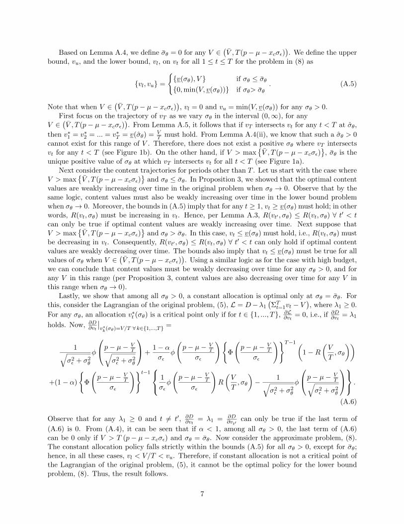
Based on Lemma A.4, we define σθ = 0 for any V ∈(V , T (p− µ− xcσε)

). We define the upper

bound, vu, and the lower bound, vl, on vt for all 1 ≤ t ≤ T for the problem in (8) as

{vl, vu} =

{{v(σθ), V } if σθ ≤ σθ{0,min(V, v(σθ))} if σθ> σθ

. (A.5)

Note that when V ∈(V , T (p− µ− xcσε)

), vl = 0 and vu = min(V, v(σθ)) for any σθ > 0.

First focus on the trajectory of vT as we vary σθ in the interval (0,∞), for anyV ∈

(V , T (p− µ− xcσε)

). From Lemma A.5, it follows that if vT intersects vt for any t < T at σθ,

then v∗1 = v∗2 = ... = v∗T = v(σθ) = VT must hold. From Lemma A.4(ii), we know that such a σθ > 0

cannot exist for this range of V . Therefore, there does not exist a positive σθ where vT intersectsvt for any t < T (see Figure 1b). On the other hand, if V > max

{V , T (p− µ− xcσε)

}, σθ is the

unique positive value of σθ at which vT intersects vt for all t < T (see Figure 1a).Next consider the content trajectories for periods other than T . Let us start with the case where

V > max{V , T (p− µ− xcσε)

}and σθ ≤ σθ. In Proposition 3, we showed that the optimal content

values are weakly increasing over time in the original problem when σθ → 0. Observe that by thesame logic, content values must also be weakly increasing over time in the lower bound problemwhen σθ → 0. Moreover, the bounds in (A.5) imply that for any t ≥ 1, vt ≥ v(σθ) must hold; in otherwords, R(vt, σθ) must be increasing in vt. Hence, per Lemma A.3, R(vt′ , σθ) ≤ R(vt, σθ) ∀ t′ < tcan only be true if optimal content values are weakly increasing over time. Next suppose thatV > max

{V , T (p− µ− xcσε)

}and σθ > σθ. In this case, vt ≤ v(σθ) must hold, i.e., R(vt, σθ) must

be decreasing in vt. Consequently, R(vt′ , σθ) ≤ R(vt, σθ) ∀ t′ < t can only hold if optimal contentvalues are weakly decreasing over time. The bounds also imply that vt ≤ v(σθ) must be true for allvalues of σθ when V ∈

(V , T (p− µ− xcσε)

). Using a similar logic as for the case with high budget,

we can conclude that content values must be weakly decreasing over time for any σθ > 0, and forany V in this range (per Proposition 3, content values are also decreasing over time for any V inthis range when σθ → 0).

Lastly, we show that among all σθ > 0, a constant allocation is optimal only at σθ = σθ. Forthis, consider the Lagrangian of the original problem, (5), L = D−λ1

(ΣTt=1vt − V

), where λ1 ≥ 0.

For any σθ, an allocation v∗t (σθ) is a critical point only if for t ∈ {1, ..., T}, ∂L∂vt

= 0, i.e., if ∂D∂vt

= λ1

holds. Now, ∂D∂vt

∣∣v∗k(σθ)=V/T ∀ k∈{1,...,T} =

1√σ2ε + σ2

θ

φ

p− µ− VT√

σ2ε + σ2

θ

+1− ασε

φ

(p− µ− V

T

σε

){Φ

(p− µ− V

T

σε

)}T−1(1−R

(V

T, σθ

))

+(1− α)

{Φ

(p− µ− V

T

σε

)}t−1 1

σεφ

(p− µ− V

T

σε

)R

(V

T, σθ

)− 1√

σ2ε + σ2

θ

φ

p− µ− VT√

σ2ε + σ2

θ

.

(A.6)

Observe that for any λ1 ≥ 0 and t 6= t′, ∂D∂vt

= λ1 = ∂D∂vt′

can only be true if the last term of

(A.6) is 0. From (A.4), it can be seen that if α < 1, among all σθ > 0, the last term of (A.6)can be 0 only if V > T (p− µ− xcσε) and σθ = σθ. Now consider the approximate problem, (8).The constant allocation policy falls strictly within the bounds (A.5) for all σθ > 0, except for σθ;hence, in all these cases, vl < V/T < vu. Therefore, if constant allocation is not a critical point ofthe Lagrangian of the original problem, (5), it cannot be the optimal policy for the lower boundproblem, (8). Thus, the result follows.

7

Proof of Theorem 2: For this proof, we fix V ≥ 2T (p − µ), σθ > 0 and vary σε. First supposethat σε = 0. Let t∗ ≥ 1 be the very first period where the content value satisfies vt∗ ≥ p−µ; hence,vt < p− µ for all t < t∗. All new customers sign up and use the service for the first time in periodt∗. Therefore, the total demand is

D = α

t∗∑t=1

Φ

(p− µ− vt

σθ

)+ (1− α) +

T∑t=t∗+1

Φ

(p− µ− vt

σθ

).

Suppose the optimal allocation is such that t∗ > 1 and it results in total demand D. Consider analternative allocation with the content values in periods t∗ and t∗− 1 reversed, that results in total

demand Dt∗,t∗−1. Observe that D − Dt∗,t∗−1 = −(1 − α)Φ(p−µ−vt∗−1

σθ

)< 0. Hence, the original

allocation with t∗ > 1 cannot be optimal. Moreover, by the same logic, the optimal allocation

must have v∗1 ≥ p − µ, resulting in demand D = αΦ(p−µ−v1σθ

)+∑T

t=2 Φ(p−µ−vtσθ

)+ 1 − α. From

the proof of Proposition 2, observe that at the maximum, ∂D∂v1

= ασθφ(p−µ−v1σθ

)must be equal to

∂D∂vt

= 1σθφ(p−µ−vtσθ

)for any t ≥ 2. Hence, there could be two possible ways in which ∂D

∂v1= ∂D

∂vtfor

any t ≥ 2 can be satisfied. First, suppose v∗1(α) > v∗t (α) such that v∗1(α) ≥ p−µ while v∗t (α) < p−µfor any t ≥ 2. If this is indeed optimal, then it must result in a higher demand compared to apolicy that divides the budget equally among all periods. Hence,

αΦ

(p− µ− v∗1(α)

σθ

)+

T∑t=2

Φ

(p− µ− v∗t (α)

σθ

)≥ αΦ

(p− µ− V/T

σθ

)+

T∑t=2

Φ

(p− µ− V/T

σθ

)

=⇒ α

[Φ

(p− µ− v∗1(α)

σθ

)− Φ

(p− µ− V/T

σθ

)]≥

T∑t=2

[Φ

(p− µ− V/T

σθ

)− Φ

(p− µ− v∗t (α)

σθ

)]

Since Φ(p−µ−v∗1(α)

σθ

)> Φ

(p−µ−V/T

σθ

)and the left hand side of the last inequality is positive,

it must also mean that, at α = 1, the allocation [v∗1(α), ..., v∗T (α)] results in a higher demandthan an equal allocation V/T in all periods. However, in Proposition 2, we proved that for anyV ≥ 2T (p−µ), an equal allocation V/T across all periods is uniquely optimal. Hence, this leads to acontradiction, and the allocation [v∗1(α), ..., v∗T (α)] cannot be optimal. The second possibility is thatv∗t (α) > v∗1(α) ≥ p−µ for any t ≥ 2. Observe that for any V ≥ 2T (p−µ), V −v∗1(α) ≥ 2(T−1)(p−µ).Therefore, per Proposition 2, v∗1(α) ≤ v∗2(α) = v∗3(α) = ... = v∗T (α) = (V − v∗1(α))/(T − 1) is theunique optimal when σε = 0 (where the first inequality is tight only at α = 1).

Next suppose that σε → 0. Following the proof of Proposition 3, consider two allocations: theoptimal allocation with vk = vH and vk+1 = vL, where vL < vH , that results in demand DHL

and an alternate allocation with vk = vL and vk+1 = vH that results in demand DLH . Note thatDLH −DHL =

= (1− α)

k−1∏j=1

Φ

(p− µ− vj

σε

)Φ

p− µ− vH√σ2ε + σ2

θ

Φ

(p− µ− vL

σε

)− Φ

p− µ− vL√σ2ε + σ2

θ

Φ

(p− µ− vH

σε

) . (A.7)

8

We discussed above that when σε = 0, the unique optimal allocation for any V ≥ 2T (p−µ) satisfiesv∗1 ≤ v∗t = V

T for all t > 1. Since (3) is right continuous at σε = 0, p−µ−vt < 0 must hold as σε → 0

for any t > 1. Observe that for any vH , vL satisfying vH > vL > p−µ, the ratioΦ(p−µ−vH

σ

)Φ(p−µ−vL

σ

) → 1 as

σ → 0 or σ → ∞ whileΦ(p−µ−vH

σ

)Φ(p−µ−vL

σ

) > 1 for all intermediate σ. Therefore, as σε → 0, DLH > DHL

for any k > 1; consequently, v∗k ≤ v∗k+1 must be true. By the above logic, v∗1 ≤ v∗2 must also holdfor σε → 0. Hence, content values must be weakly increasing over time for σε → 0.

Next suppose σε →∞. When σε →∞, σθσε → 0. From (A.7), observe that for σε →∞, we have

that ∂∂σ

Φ(p−µ−vH

σ

)Φ(p−µ−vL

σ

)∣∣∣∣∣σ=σε

< 0 implies that DLH −DHL < 0. Now,

∂

∂σ

Φ(p−µ−vH

σ

)Φ(p−µ−vL

σ

) ∣∣∣∣∣σ=σε

=1

σε

Φ(p−µ−vH

σ

)Φ(p−µ−vL

σ

) [g(p− µ− vHσε

)− g

(p− µ− vL

σε

)].

The generalized failure rate of the standard normal distribution, g(x), decreases in (−∞, xc] andincreases in [xc,+∞). Since σε →∞, we have that xc <

p−µ−vHσε

< p−µ−vLσε

for any vH > vL; hence,

∂∂σ

Φ(p−µ−vH

σ

)Φ(p−µ−vL

σ

)∣∣∣∣∣σ=σε

< 0. Therefore, DLH < DHL for any k ≥ 1 and vH > vL; consequently, content

values must be weakly decreasing over time for σε →∞.For intermediate values of σε, we provide a proof similar to that of Theorem 1. For a fixed

σθ > 0, let R(v, σε) =Φ

(p−µ−v√σ2ε+σ

2θ

)Φ(p−µ−vσε

) . We showed in Lemma A.3 that for the optimal allocation (to

the approximate and original problems), R(vk, σε) ≤ R(vk+1, σε) for any k ≥ 1 must hold. FromLemma A.4, note that when σε ≥ p−µ

xc, ∂∂vR(v, σε) < 0 for any v ≤ p−µ−xcσε, while ∂

∂vR(v, σε) > 0

for any v ≥ p − µ − xc√σ2ε + σ2

θ . Therefore, R(v, σε) must have a unique minimum, v(σε), in the

interval(p− µ− xcσε, p− µ− xc

√σ2ε + σ2

θ

)satisfying g

(p−µ−v(σε)

σε

)= g

(p−µ−v(σε)√

σ2ε+σ2

θ

).

To see how the unique minimum, v(σε), changes with σε, we differentiate both sides of the

equality g(p−µ−v(σε)

σε

)= g

(p−µ−v(σε)√

σ2ε+σ2

θ

)with respect to σε to obtain

dv(σε)

dσε=

σ2ε

σ2ε+σ2

θ

p−µ−v(σε)√σ2ε+σ2

θ

∂∂vg

(p−µ−v√σ2ε+σ2

θ

) ∣∣∣∣v=v(σε)

− p−µ−v(σε)σε

∂∂vg

(p−µ−vσε

) ∣∣∣∣v=v(σε)

∂∂vg

(p−µ−vσε

) ∣∣∣∣v=v(σε)

− σε√σ2ε+σ2

θ

∂∂vg

(p−µ−v√σ2ε+σ2

θ

) ∣∣∣∣v=v(σε)

.

Noting that ∂∂vg

(p−µ−v√σ2ε+σ2

θ

) ∣∣∣∣v=v(σε)

< 0, ∂∂vg

(p−µ−vσε

) ∣∣∣∣v=v(σε)

> 0, p−µ−v(σθ)√σ2ε+σ2

θ

< 0, and p−µ−v(σε)σε

<

0, we conclude that dv(σε)dσε

> 0.

On the other hand, if σε <p−µxc

and g

(p−µ√σ2ε+σ2

θ

)< g

(p−µσε

), ∂∂vR(v, σε) > 0 for any v ≥ 0. If we

increase σε such that p−µσε

< xc <p−µ√σ2ε+σ2

θ

< 0 and g

(p−µ√σ2ε+σ2

θ

)≥ g

(p−µσε

), then ∂

∂vR(v, σε)∣∣v=0≤ 0

9

holds. Hence, in this case, as long as σε is large enough, we can use similar arguments to show

that R(v, σε) has a unique minimum v(σε) ∈[0, p− µ− xc

√σ2ε + σ2

θ

)that strictly increases with

σε. Combining the two cases, σε <p−µxc

and σε ≥ p−µxc

, we can conclude that as long as σε is abovea threshold, R(v, σε) has a unique minimum, v(σε), that starts at 0 and strictly increases with σε.Let σε be the unique value of σε that satisfies v(σε) = V/T .

From Lemma A.5, observe that an intersection can only occur at a minimum, v(σε). Moreover,for any 1 ≤ t′ < t ≤ T , if vt and vt′ intersect at σε, then at σε, v1 = v2 = ... = vk = v(σε) musthold. Similar to (A.5), we again define the upper bound, vu, and the lower bound, vl, on vt for all1 ≤ t ≤ T for the lower bound problem as

{vl, vu} =

{{v(σε), V } if σε ≤ σε{0,min(V, v(σε))} if σε > σε

. (A.8)

We discussed above that content values are weakly increasing over time when σε → 0 andweakly decreasing when σε → ∞. It follows that σε is the unique positive value of σε at whichthe trajectory of vT can intersect with any other vt; and at σε, v1 = ... = vT = V/T. Using asimilar logic as in the proof of Theorem 1, it follows that, under the constraints vl ≤ vt ≤ vu forall t ≥ 1, an intersection between content trajectories for periods t < T and t′ < t violates thecondition R(vt′ , σε) ≤ R(vt, σε). Hence, no other intersection can occur. Furthermore, using (A.6),we can similarly argue that if α < 1, among all σε > 0, σε = σε is the only point where a constantallocation with v∗t (σε) = V/T is optimal. Thus, the result follows.

Proof of Proposition 5: We start with the effect of α on the provider’s optimal allocation. Letthe total demand over the planning horizon from new customers be DN . Hence, the total demandin the planning horizon is

D(α) = α

Φ

p− µ− v1√σ2ε + σ2

θ

+ Φ

p− µ− V + v1√σ2ε + σ2

θ

+ (1− α)DN .

For any α, the optimal values, v∗1(α) and V − v∗1(α), must be such that dD(α)dv1

∣∣∣∣∣v∗1(α)

=

= (1− α)dDN

dv1

∣∣∣∣∣v∗1(α)

+α√

σ2ε + σ2

θ

φp− µ− v1√

σ2ε + σ2

θ

− φp− µ− V + v1√

σ2ε + σ2

θ

∣∣∣∣∣v∗1(α)

= 0. (A.9)

Since µ+V/2−p > 0, for any v1 < V/2,∣∣∣ p−µ−v1√

σ2ε+σ2

θ

∣∣∣ < ∣∣∣p−µ−V+v1√σ2ε+σ2

θ

∣∣∣; consequently, φ

(p−µ−v1√σ2ε+σ2

θ

)>

φ

(p−µ−V+v1√

σ2ε+σ2

θ

). Therefore, for any v∗1(α) < V/2, d

dv1

[Φ

(p−µ−v1√σ2ε+σ2

θ

)+ Φ

(p−µ−V+v1√

σ2ε+σ2

θ

)] ∣∣∣∣∣v∗1(α)

> 0,

while dDN

dv1

∣∣∣v∗1(α)

< 0. From (A.9) it also follows thatdv∗1(α)dα = −

∂2D(α)∂v1∂α

∣∣∣v∗1(α)

∂2D(α)

∂v21

∣∣∣v∗1(α)

. Since v∗1(α) is a local

maximum, ∂2D(α)∂v21

∣∣∣v∗1(α)

< 0. On the other hand, dDN

dv1

∣∣∣v∗1(α)

< 0 and

10

ddv1

[Φ

(p−µ−v1√σ2ε+σ2

θ

)+ Φ

(p−µ−V+v1√

σ2ε+σ2

θ

)] ∣∣∣∣∣v∗1(α)

> 0 imply ∂2D(α)∂v1∂α

∣∣∣v∗1(α) > 0. Therefore, for any v∗1(α) <

V/2,dv∗1(α)dα > 0. However, if v∗1(α) > V/2, d

dv1

[Φ

(p−µ−v1√σ2ε+σ2

θ

)+ Φ

(p−µ−V+v1√

σ2ε+σ2

θ

)] ∣∣∣v∗1(α)

< 0, while

dDN

dv1

∣∣∣v∗1(α)

> 0. Using similar arguments, we conclude that for any v∗1(α) > V/2,dv∗1(α)dα < 0.

Therefore, as α increases, v∗1(α) moves closer to V/2, and |v∗1(α)− v∗2(α)| weakly decreases.Next focus on the effect of α on the total demand. First observe from (3) that new customer

demand when v∗1 = V/2 is

DN |v∗1=V/2 = 1− Φ2

(p− µ− V

2

σε

)+ Φ

p− µ− V2√

σ2ε + σ2

θ

Φ

(p− µ− V

2

σε

)≥ 2Φ

p− µ− V2√

σ2ε + σ2

θ

.

The last inequality follows from the fact that for any µ+ V/2 > p, Φ

(p−µ−V

2√σ2ε+σ2

θ

)≤ Φ

(p−µ−V

2σε

).

Let us again start with the case where v∗1(α) < V/2. We showed above that for this range

of v∗1(α), v∗1(α) weakly increases with α and the new customer demand dDN

dv1

∣∣∣v∗1(α)

< 0. From

Proposition 2, it follows that v∗1(α = 1) = V/2. Therefore for any α ≤ 1,

DN |v∗1(α) ≥ DN |V/2 ≥ 2Φ

p− µ− V2√

σ2ε + σ2

θ

. (A.10)

Additionally, when v∗1(α) < V/2, ddv1

[Φ

(p−µ−v1√σ2ε+σ2

θ

)+ Φ

(p−µ−V+v1√

σ2ε+σ2

θ

)] ∣∣∣v∗1(α)

> 0 for all α. Hence,

Φ

p− µ− v1√σ2ε + σ2

θ

+ Φ

p− µ− V + v1√σ2ε + σ2

θ

∣∣∣∣∣v∗1(α)

≤ 2Φ

p− µ− V2√

σ2ε + σ2

θ

. (A.11)

(A.10) and (A.11) must imply that whenever v∗1(α) < V/2,

DN |v∗1(α) ≥

Φ

p− µ− v1√σ2ε + σ2

θ

+ Φ

p− µ− V + v1√σ2ε + σ2

θ

∣∣∣∣∣v∗1(α)

(A.12)

Now consider two values of α, αL and αH > αL. The total demand then satisfies D(αL, v∗1(αL))−

D(αH , v∗1(αH))≥D(αL, v

∗1(αH))−D(αH , v

∗1(αH)) =

= (αH − αL)

DN |v∗1(αH) −

Φ

p− µ− v1√σ2ε + σ2

θ

+ Φ

p− µ− V + v1√σ2ε + σ2

θ

∣∣∣∣∣v∗1(αH)

≥ 0.

The first inequality follows from the fact that D(αL, v∗1(αL)) ≥ D(αL, v

∗1(αH)) while the second

inequality follows from (A.12).

On the other hand, when v∗1(α) > V/2, ddv1

[Φ

(p−µ−v1√σ2ε+σ2

θ

)+ Φ

(p−µ−V+v1√

σ2ε+σ2

θ

)] ∣∣∣v∗1(α)

< 0 while

11

dDN

dv1

∣∣∣v∗1(α)

> 0; but v∗1(α) decreases with α. We can use similar arguments to show that the

inequality D(αL, v∗1(αL)) ≥ D(αH , v

∗1(αH)) holds.

Proof of Proposition 6: When T = 2 and σθ = 0, we can substitute v2 = V − v1 and observe

that v∗1 = V/2 is the unique global maximum to D = Φ(p−µ−v1

σε

)+ Φ

(p−µ−(V−v1)

σε

)for any

V > 2(p− µ). Hence, when T = 2, the threshold on budget is V = 2(p− µ) for p > µ.As V → 2(p − µ), we have that (p − µ − v1) + (p − µ − V + v1) → 0 for any v1 ≤ V . Hence,

limV→2(p−µ)

[φ

(p−µ−v1√σ2ε+σ2

θ

)− φ

(p−µ−V+v1√

σ2ε+σ2

θ

)]= 0 and limV→2(p−µ)

[φ(p−µ−v1

σε

)− φ

(p−µ−V+v1

σε

)]=

0. Moreover, from Theorem 1, we have that v∗1 ≥ V/2 in this case; so, p− µ− V + v1 ≥ 0. Now,

dD

dv1=

α√σ2ε + σ2

θ

φp− µ− v1√

σ2ε + σ2

θ

− φp− µ− V + v1√

σ2ε + σ2

θ

+ (1− α)

[1

σεφ

(p− µ− v1

σε

)Φ

(p− µ− V + v1

σε

)− 1

σεφ

(p− µ− V + v1

σε

)Φ

(p− µ− v1

σε

)]

+(1−α)

+1

σεφ

(p− µ− v1

σε

)Φ

p− µ− V + v1√σ2ε + σ2

θ

− 1√σ2ε + σ2

θ

φ

p− µ− V + v1√σ2ε + σ2

θ

Φ

(p− µ− v1

σε

) .Hence, limV→2(p−µ)

dDdv1≥ limV→2(p−µ)(1−α)Φ

(p−µ−v1

σε

)[1σεφ(p−µ−V+v1

σε

)− 1√

σ2ε+σ2

θ

φ

(p−µ−V+v1√

σ2ε+σ2

θ

)].

Moreover, 1σφ( aσ ) decreases with σ whenever a2

σ2 ≤ 1. Therefore, limV→2(p−µ)dDdv1≥ 0 whenever

limV→2(p−µ)p−µ−V+v1

σε≤ 1. Thus, when V → 2(p− µ), the optimal period 1 content value is such

that limV→2(p−µ) v∗1 ≥ V

(12 + σε

2(p−µ)

).

For part (ii), note that when V →∞, the allocation v∗1 = v∗2 = V/2 results in limV→∞D|v∗1=V/2 =2, and the demand cannot be improved by any other allocation policy. Hence, the result follows.

12