University of Pennsylvania University of Pennsylvania

ScholarlyCommons ScholarlyCommons

Finance Papers Wharton Faculty Research

2-1-2015

Intertemporal Information Acquisition and Investment Dynamics Intertemporal Information Acquisition and Investment Dynamics

Christian C. Opp University of Pennsylvania

Follow this and additional works at: https://repository.upenn.edu/fnce_papers

Part of the Finance and Financial Management Commons

Recommended Citation Recommended Citation Opp, C. C. (2015). Intertemporal Information Acquisition and Investment Dynamics. SSRN's eLibrary, http://dx.doi.org/Opp, Christian C., Intertemporal Information Acquisition and Investment Dynamics (February 1, 2015). Available at SSRN: https://ssrn.com/abstract=2587852 or http://dx.doi.org/10.2139/ssrn.2587852

This paper is posted at ScholarlyCommons. https://repository.upenn.edu/fnce_papers/10 For more information, please contact repository@pobox.upenn.edu.

Intertemporal Information Acquisition and Investment Dynamics Intertemporal Information Acquisition and Investment Dynamics

Abstract Abstract This paper studies intertemporal information acquisition by agents that are rational Bayesian learners and that dynamically optimize over consumption, investment in capital, and investment in information. The model predicts that investors acquire more information in times when future capital productivity is expected to be high, the cost of capital is low, new technologies are expected to have a persistent impact on productivity, and the scalability of investments is expected to be high. My results shed light on the economic mechanisms behind various dynamic aspects of information production by the financial sector, such as the sources of variation in returns on information acquisition for investment banks or private equity funds.

Keywords Keywords dynamic information acquisition, investment, asset markets, bayesian learning

Disciplines Disciplines Business | Finance and Financial Management

This working paper is available at ScholarlyCommons: https://repository.upenn.edu/fnce_papers/10

Electronic copy available at: http://ssrn.com/abstract=2587852

Intertemporal Information Acquisition and

Investment Dynamics

Christian C. G. Opp∗

February 2015

Abstract

The paper studies intertemporal information acquisition by agentsthat are rational Bayesian learners and that dynamically optimize overconsumption, investment in capital, and investment in information. Themodel predicts that investors acquire more information in times when fu-ture capital productivity is expected to be high, the cost of capital is low,new technologies are expected to have a persistent impact on productiv-ity, and the scalability of investments is expected to be high. My resultsshed light on the economic mechanisms behind various dynamic aspectsof information production by the financial sector, such as the sources ofvariation in returns on information acquisition for investment banks orprivate equity funds.

JEL topic area codes: C61, D83, D91, D92, G24

1 Introduction

The investors’ conditional information sets drive the dynamics of both as-set prices and investment. Which economic factors determine the evolution ofthe information sets? The asset pricing literature typically takes the informa-tion flow to investors as exogenous and uses various instruments to capture thedynamics of the information set.

In this paper, I endogenize the information set and explore the economicdeterminants of intertemporal information acquisition decisions. I develop adynamic model in which investors are Bayesian learners who optimally choosehow much to consume, how much to invest, and how much information to ac-quire. This model reveals various links between the investors’ efforts to learn

∗The Wharton School, University of Pennsylvania. Email: opp@wharton.upenn.edu. Thispaper was developed during my time in the Chicago Booth Ph.D. program. I thank JohnCochrane, John Heaton, Atif Mian, Thomas Sargent, Harald Uhlig, Pietro Veronesi, ArnoldZellner, and in particular my advisors Lars Hansen and Lubos Pastor, for outstanding supportand feedback. This research was funded in part by the Best Foundation’s Arnold Zellner Doc-toral Prize and by grants from the German National Academic Foundation and the GermanAcademic Exchange Service (DAAD).

1

Electronic copy available at: http://ssrn.com/abstract=2587852

about new technologies and their conditional expectations on productivity, dis-count factors, and scale economies.

The model predicts that investors acquire more information when futurecapital productivity is expected to be high, expected returns are low, technologychanges are expected to have a persistent impact on productivity, and futureinvestment scalability, as for example influenced by liquidity, is expected to behigh. Economic mechanisms that decrease the scalability of investment diminishthe marginal gains from information acquisition since they restrict the flexibilityto respond to news.

The results imply various predictions on the determinants of variation inknowledge acquisition by the financial service sector. Since human capital istypically the scarce factor in information production, compensation and hiringand firing decisions are expected to be linked to changes in financial institu-tions’ expectations about future productivity, persistence of technologies, andliquidity. Further, the theory rationalizes private equity and hedge funds’ pref-erence for long-term capital commitments: lower dependence on future capitalcontributions gives the funds greater flexibility in intertemporal investment de-cisions. This increases returns on information acquisition. Firms that are morefinancially constrained are predicted to benefit less from information acquisitionand thus will prefer to stay less informed. Further, private equity funds are pre-dicted to stay less informed if they expect a less liquid IPO market and lowercapital productivity in the future.

Generally, variants of the presented model might be useful to analyze dif-ferences in the information production technologies across investment firms andthe corresponding determinants of the latent evolution of knowledge and in-vestment skill. In addition, on a more aggregated level, the model could beused to analyze differences in the information acquisition technologies availableto investors across countries, which could be useful for policy considerations:the framework links the characteristics of the information acquisition technol-ogy available to investors in a financial system to intertemporal investment andconsumption allocations. This allows analyzing the impact of frictions to theintertemporal scalability of information acquisition, for example as imposed bylabor market regulations, and changes in cost levels, for example as induced byaccounting regulations.

Model Approach

To make the analysis tractable the presented model uses a reduced formrepresentation of the equilibrium in the information market: an informationacquisition technology subsumes various economic mechanisms that have animpact on the information acquisition cost faced by investors. A sequentialjoint consumption, investment, information acquisition problem is analyzed fora general time- and state-dependent information acquisition cost function andthe class of additively separable preferences.

The resulting intertemporal optimality condition for information acquisitionshows that the marginal return on uncertainty reduction satisfies - like all other

2

asset returns - the Euler equation, suggesting the interpretation of informationas an asset. The paper explores the dynamic relation between the marginalreturn on this asset and technology changes.

Literature

Bayesian learning is an essential component of the presented framework.The literature on asset market dynamics caused by learning typically considersan exogenous evolution of information. Examples include Pastor and Veronesi[1] and Hansen[2].1 A key distinction from this literature is the paper’s focuson active information acquisition decisions which make the information flow toagents endogenous.

Noisy rational expectations models in the spirit of Grossman and Stiglitz[10] are traditionally used to analyze information acquisition in finance (Verrec-chia [11]; Barlevy and Veronesi [12]; Peress [13]; Veldkamp [14]). These modelstypically focus on aspects of asymmetric information and decentralization instatic environments.2 When applied to the analysis of joint dynamics in infor-mation acquisition, investment, and consumption this type of setup quickly losestractability despite restrictive assumptions about information cost structures,production technologies, and preferences. As shown later, the predictions of thispaper arise through the analysis of a dynamic setup with richer specificationsof technologies.

The paper shares with the recent literature on “rational inattention” (e.g.,Sims [16], [17]; Luo [18]; Turmuhambetova [19]) that a dynamic setup is consid-ered where information used by agents is endogenous. Yet, in contrast to theliterature following Sims this paper does not model how an individual allocatesher limited capacity to process available information. The literature follow-ing Sims is “motivated by the idea that information that is freely available toan individual may not be used, because of the individual’s limited informationprocessing capacity” [20]. In contrast, this paper considers producers of infor-mation, like financial institutions that develop information that is not freelyavailable at the time when it is used or sold. Financial institutions hire employ-ees who use available information in combination with costly investigation toproduce proprietary estimates of relevant investment measures. Sims explicitlyexcludes actions of “costly investigation”[20], such as interviewing experts ontechnologies and consumer surveys, from the activities where the constraintsmodeled in the rational inattention framework are of relevance. In this paperinformation acquisition cost refer to the full cost of developing information, suchas the cost of labor, IT infrastructure, and physical assets. It is not the shadowprice of a constraint to pay attention to information that an individual already

1Other papers on robust control are e.g., Hansen, Sargent and Tallarini [3], Hansen andSargent ([4], [5]) and Hansen, Sargent and Wang [6]). Learning is also a central concept toother parts of the recent finance literature such as Pastor and Veronesi [7] (learning aboutprofitability), Lewellen and Shanken [8] (learning and asset pricing tests), Adrian and Franzoni[9] (learning about time-varying factor loadings).

2Wang [15] considers a dynamic setup with asymmetric information but keeps informationexogenous.

3

has at her disposal.3 This conceptually different focus leads to a different modelapproach. Agents are Bayesian learners that form rational expectations condi-tional on all information that is available to them.

Finally, Abel, Eberly, and Panageas [21] consider a setup where inattentiveagents update their information sporadically, rather than continuously. Opti-mally inattentive behavior is generated by the assumption that the consumermust pay a cost that is proportional to the portfolio’s contemporaneous valueto observe the value of his investment portfolio. The consumer optimally checkshis investment portfolio at equally spaced points in time, consuming from ariskless transactions account in the interim.

The paper proceeds as follows: the next Section builds a model of jointconsumption, investment, and information acquisition decisions in a productioneconomy with time varying technology risk. Intertemporal optimality conditionsare presented and economic determinants of information acquisition by Bayesianlearners are examined. The model’s predictions are discussed in reference todynamic aspects of information production by the financial sector. Section 3concludes.

2 Model

2.1 Production Technology

Consider a decision maker who may invest in a project with weakly decreas-ing returns to scale. Let Ft denote the decision maker’s information set at datet, Yt denote output at date t measured in terms of a single composite con-sumption good, and Gt (·) be a strictly increasing, concave, and Ft-measurablefunction. Given risky capital kt at date t, output at date (t+ 1) is determinedby the following relation:

Yt+1 = At+1Gt (kt) . (1)

In equation (1) the parameter At+1 is stochastic conditional on the informationset Ft. Ex post, at date (t+ 1) , the decision maker may infer the actual re-alization of At+1 based on the observed output Yt+1 and the choice of kt. Letεt = (εa,t, εs,t, εµ,t, εz,t)

′be an i.i.d. Gaussian shock process with mean zero

and identity covariance matrix. The productivity factor At is assumed to havethe following exponential affine structure

at ≡ logAt = ωa + µt + σvεa,t, (2)

where ωa sets the unconditional mean of at, µt is a stationary hidden statecomponent with unconditional mean zero, and εa,t is an independent shock toproductivity that prevents the full revelation of the hidden state µt through the

3Even though employees’ limits to pay attention to information they already have mayinfluence their productivity this is likely not a central aspect for the analysis of financialinstitutions. Sims [20] supports this view by stating that “sophisticated, continuously tradinginvestors have uncertainty that is dominated by information that is not freely available”.

4

output realization Yt. σv is an exogenous scalar that determines the exposureof productivity to unpredicTable noise εa,t. In this paper a stationary economyis considered where the exogenous parameters ωa and σv are specified as time-invariant. Yet, the derivation in the Appendix accommodates time variationsuch that the analysis may be extended to study aspects like growth. Further,for notational simplicity the time subscript on the Gt (·) function will usuallybe suppressed in the following exposition. For the stochastic simulation of themodel that is presented below a Cobb-Douglas specification of the productionfunction is considered which yields the following representation:

Yt+1 = At+1k1−ηt with 0 ≤ η < 1. (3)

In this specification the parameter η corresponds to the local curvature of theproduction technology.

Production Technology Risk

Empirical evidence suggests that the exposure of economies to technologyrisk exhibits time-variation (see e.g., Ng et al. [22]): during the internet orbiotech “revolutions” (Pastor and Veronesi [1]) in the 1980s and 1990s economieslike the US were exposed to substantial technological change and correspondinghigh levels of technological uncertainty. Investors were confronted with thetask to predict the impact of the new technologies on productivity in the short,medium, and long run in order to make investment decisions. To do so they hadto acquire information that allowed them to forecast changes in product markets,consumer behavior, and business prospects. The blooming of the profession ofinvestment analysts during these times is anecdotal evidence for the increase inaggregate demand for information acquisition capacities. In contrast, in othertimes like in the years post 2000/2001 the capacities of analysts were markedlyreduced, resulting in the well known layoff waves in the financial sector.

For a theory on dynamics in information acquisition by investors time-variation in technology risk thus seems to be an essential ingredient. In themodel the notion of time varying exposures to technology risk is captured bythe specification of the evolution of µt, the persistent component of log produc-tivity at. Technology risk therefore refers to shocks that also have an impact onproductivity in future periods. It is this feature that makes “new technologies”a learning target for investors. In particular, µt is assumed to follow a stationaryMarkov process that is mean reverting to zero:

µt+1 = φµµt + σµ,tεµ,t+1 , 0 ≤ φµ < 1. (4)

The time-varying exposure to technology risk σ2µ,t is governed by the Markov

state zt which evolves according to the following stationary process:

zt+1 = ωz + φzzt + σzεz,t+1, 0 ≤ φz < 1. (5)

A Ft−measurable, positive-valued function σ2µ,t (zt) maps the state zt into a risk

exposure σ2µ,t. For the simulation results that are presented later in the paper

5

an EGARCH type of specification (Nelson [23]) of the function σ2µ,t (zt) is used:

σ2µ,t = ϕσ exp zt , ϕσ > 0. (6)

2.2 Information Acquisition Technology

In reality, a variety of economic factors have an impact on the informationacquisition technology available to investors. Essentially the financial system asa whole determines the cost of acquiring information on projects in the economy:laws and regulations, the accounting system with institutions like the SEC, thedevelopment of the banking system and financial intermediaries, availability ofhuman capital, and the micro-structure of stock markets and trading platforms,to mention only a short list of potentially relevant factors.

A broad finance and accounting literature suggests that a system of efficientdisclosure rules, financial intermediaries (Diamond [24]), and financial contracts(Townsend [25]) reduces information asymmetries and mitigates the duplicationof effort. Law systems influence corporate governance and investors’ facility tomonitor a company’s operations and outcomes in timely fashion (La Porta etal. [26]; D’Avolio et al. [27]; Dyck et al. [28]).4 Trading technologies and thestructure of information markets influence the dissemination and aggregationof information held by market participants and thus the cost of information ac-quisition faced by investors (Diamond and Verrecchia [29]; Hellwig [30]; Admati[31]; Admati and Pfleiderer [32], [33], [34]; Veldkamp [14]).

In order not to get lost in the variety of these mechanisms and to maintaina focus on joint dynamics in investment, consumption, and information acquisi-tion this paper proposes a reduced form approach to characterize the informa-tion acquisition technology available to investors. The technology, specified bya cost function over information precision, subsumes various economic mecha-nisms that determine the costliness of information, including effects induced byinformational externalities. The cost structure is the outcome of equilibria inother markets that are of relevance for information acquisition, or in short bythe “information market.” The decision maker takes this cost structure as ex-ogenously given. Quantity decisions are assumed to be not publicly observable.The price of capital is equal to one in terms of the composite consumption goodand does not signal additional information.

In terms of the model the decision maker may influence the precision of asignal st that she obtains jointly with the production output at the end of eachperiod. The signal structure is specified as follows:

st+1 = µt+1 +σv√ιtεs,t+1. (7)

The strictly positive and continuous decision variable ιt controls informationacquisition by scaling the noise variance of the signal st+1. Obtaining one signal

4Laws also influence investors’ protection against expropriation by insiders and corporategovernance control rights.

6

with noise variance σ2v/ιt is informationally equivalent to obtaining ιt separate,

independent signals with noise variance σ2v ; conditional uncertainty is reduced

by the same amount. Since the parameter σv is common to the specificationsof st+1 and at+1 the scaling implies that choosing ιt = 1 corresponds to theacquisition of information that has the same signal-to-noise ratio as the period’slog-productivity realization at+1.

The cost of acquiring a signal st+1 with noise variance σ2v,t/ιt is specified

by the function nt (ιt). The model is analyzed for a general time and statedependent,5 strictly increasing and convex cost function which is required tosatisfy n′t (ιt)|ιt=0 = 0, for all t, to ensure strictly positive choices of ι. Theconvexity of nt (ιt) reflects the notion that acquiring an additional independentsignal becomes more costly the more information is acquired in a given period.For the simulation of the model, the following functional form will be considered:

nt (ιt) =χ

κ+ 1· ικ+1t , with κ ≥ 0 and χ > 0. (8)

The specification features two properties of an information acquisition technol-ogy: the marginal cost of information acquisition and the costliness of varyinglearning effort intertemporally. The parameter χ shifts the marginal cost, theparameter κ influences the local curvature of nt (ιt).

Bayesian Updating

Due to the conditional knowledge of the Markov state zt which governsthe risk exposures σ2

µ,t a version of Kalman filtering with time varying signalprecision is applicable. As a Bayesian learner, the agent updates his beliefs aboutthe hidden productivity state based on observed realizations of the randomvariables at and st. Let (at, st) denote the whole history of signals that thedecision maker obtained up to date t, i.e.,(

at, st)≡ (at, st) , (at−1, st−1) , (at−2, st−2) , · · · ,

and define the conditional mean µt ≡ E [µt+1| at, st] and the conditional vari-ance σ2

t ≡ V ar [µt+1| at, st]. Given the initial prior distribution of the hiddenproductivity state is normal, µ1 ∼ N

(µ0, σ

20

), the posterior density at date

t is also normal, µt+1 ∼ N(µt, σ

2t

), where the conditional mean µt and the

conditional variance σ2t follow from the Kalman filter recursions:

µt = φµat − ωa,t−1 + ιt−1st +

σ2v

σ2t−1

µt−1

1 + ιt−1 +σ2v

σ2t−1

(9a)

σ2t ≡ V ar

[µt+1| at, st

]= σ2

µ,t + σ2p,t, (9b)

5It is required that the state that governs variation in the functional form of nt (ιt) isexogenous to the decision maker.

7

where σ2p,t denotes the pre-shock conditional variance at time t which is defined

as follows:

σ2p,t

(σ2t−1, ιt−1

)≡ φ2

µ

σ2v

1 + ιt−1 +σ2v

σ2t−1

. (10)

2.3 Decision Problem

The decision maker solves a sequential joint consumption-, investment-, in-formation acquisition problem. Choices are ranked by von Neumann Morgen-stern preferences. Let βt ∈ (0, 1) be a Ft−measurable discount factor for thetime period from t to (t+ 1) and F (ct) be a strictly increasing and concaveone-period utility function. Further, let yt ≡ log Yt denote log-output. Givenan initial state vector x0 ≡

(y0, µ0, σ

2p,0, z0

)′, consider the sequential problem

to maximize

F (ct) + Et

∞∑j=1

(j−1∏i=0

βt+i

)F (ct+j) (11)

subject to the budget restriction

ct = Yt − kt − nt (ιt) (12)

and the transition laws and technologies specified in equations (1) - (10). Asso-ciated with this problem is the Bellman equation

V (xt) = maxut=(kt,ιt)

′F (ct) + βtE [V (xt+1) |xt,ut] (13)

with the vector of state variables xt ≡(yt, µt, σ

2p,t, zt

)′, and the vector of con-

trols ut≡ (kt, ιt)′, and where V (xt) denotes the optimal value of the objective

function (11) starting from state xt. E [·|xt,ut] denotes the mathematical ex-pectation given the vectors (xt,ut) which yield a sufficient statistic for theconditional distribution of the next period state xt+1. While µt and σ2

p,t char-acterize the conditional distribution of the hidden state µt+1, the observableMarkov state zt determines the distribution of the next period technology riskexposure σ2

µ (zt+1). The state vector transition equations are given below.

yt+1 = at+1 + logGt (kt)

µt+1 = φµat+1−ωa,t+ιtst+1+

σ2vσ2tµt

1+ιt+σ2vσ2t

σ2p,t+1 = φ2

µσ2v

1+ιt+σ2vσ2t

zt+1 = ωz + φzzt + σzεz,t+1

(14)

8

2.4 Optimality Conditions

The envelope condition and the first order necessary condition for capital ktyield the familiar Euler equation

E [At+1G′ (kt)mt+1|xt,ut] = 1, (15)

where mt+1 ≡ βtF′(ct+1)

F ′(ct)denotes the stochastic discount factor and At+1G

′ (kt)

the marginal gross return on capital. Note that information acquisition decisionsplay a central role in the Euler equation: by controlling information acquisitionι, the investor influences the evolution of the conditional information set andthus the conditional expectations operator in the Euler equation (15). Dynam-ics in asset prices are thus directly linked to decisions on ι and their economicdeterminants. This is a key distinction from the existing literature that analyzesdynamics induced by Bayesian learning but takes the information flow as ex-ogenous. In reference to the language used in empirical asset pricing, the set ofsignals obtained by the investor may be viewed as an “endogenous instrument”that summarizes conditional information.

Optimization generates restrictions on intertemporal information acquisitionand thus on the information flow to investors. Let λ denote Lebesgue measureand f (at+1, st+1, εz,t+1|xt,ut) the joint conditional probability density func-tion of the vector (at+1, st+1, εz,t+1)

′. The first order necessary condition for

information acquisition ιt may be written as follows:

n′t (ιt)F′ (ct)

βt(16)

=

∫ (∂µt+1

∂ιt

∂V (xt+1)

∂µt+1+∂σ2

p,t+1

∂ιt

∂V (xt+1)

∂σ2p,t+1

)·

f (at+1, st+1, εz,t+1|xt,ut) dλ (at+1, st+1, εz,t+1) +∫V (xt+1)

∂f (at+1, st+1, εz,t+1|xt,ut)∂ιt

dλ (at+1, st+1, εz,t+1)

where µt+1 = µt+1

(at+1, st+1, µt, σ

2t , ιt

)and σ2

p,t+1 = σ2p,t+1

(σ2t , ιt

). The fol-

lowing Proposition gives the associated necessary intertemporal optimality con-dition.

Proposition 1. The decision problem associated with the Bellman equation (13)implies the following necessary intertemporal condition for optimal informationacquisition ι :

Et

[mt+1

Πt+1 + δt+1MCt+1

(σ2p,t+2

)MCt

(σ2p,t+1

) ]= 1 (17)

where mt+1 = βtF′(ct+1)

F ′(ct)denotes the stochastic discount factor and the following

9

definitions apply

Πt+1 ≡ 1

2

∂2V (xt+1)∂µ2

t+1− ∂2V RS(xt+1,ut+1)

∂µ2t+1

F ′ (ct+1)

=1

2

∂2V RS(xt+1,ut+1)∂µt+1∂kt+1

∂kt+1(xt+1)∂µt+1

+∂2V RS(xt+1,ut+1)

∂µt+1∂ιt+1

∂ιt+1(xt+1)∂µt+1

F ′ (ct+1)

MCt(σ2p,t+1

)≡ n′t (ιt)

/−∂σ2

p,t+1

(σ2t , ιt

)∂ιt

∂σ2p,t+1

(σ2t , ιt

)∂ιt

≡ −φ2µσ

2v,t(

1 + ιt +σ2v,t

σ2t

)2

δt+1 ≡∂σ2

p,t+2

(σ2t+1, ιt+1

)∂σ2

t+1

=φ2µ(

1 + (1 + ιt+1)σ2t+1

σ2v

)2

and where V RS(xt+1,ut+1

)denotes the right side of the Bellman equation (13)

evaluated at the optimal policy rule u (xt+1).

Proof. See Appendix.

Discussion of Proposition 1

Equation (17) indicates that at the optimum, the marginal return on uncer-tainty reduction satisfies an Euler equation: current marginal cost of reducinguncertainty, denoted by MCt

(σ2p,t+1

), are compensated by a future, stochastic

benefit which may be decomposed into two components: Πt+1, which is accru-ing at time (t+ 1), and subsequent benefits of value δt+1MCt+1

(σ2p,t+2

), where

δt+1 captures the notion of depreciation of information. The structure of thismarginal return is similar to the one of a return on capital where the next pe-riod benefit consists of a dividend payment and a remaining depreciated capitalvalue. The representation suggests that marginal uncertainty reduction inducedby information acquisition may be viewed as an asset that generates a streamof benefits in future periods. In the following, the terms in equation (17) arediscussed in more detail.

Πt+1 : Marginal Next Period Benefit of Uncertainty Reduction

Πt+1, the marginal next period benefit of uncertainty reduction, is generatedby state-contingent adjustments to tomorrow’s controls u (xt+1) in reaction to amore precise productivity estimate. Aversion against uncertainty about the nextperiod productivity estimate µt+1, as represented by the curvature of the valuefunction

(∂2V (xt+1) /∂µ2

t+1

), is alleviated by additional information acquisition

since next period’s decisions optimally take into account additional information.SubSection 2.5 considers an approximation of Πt+1 which sheds more light onthe economic determinants of this term.

10

MCt(σ2p,t+1

): Marginal Cost of Uncertainty Reduction

MCt(σ2p,t+1

)denotes the marginal cost of reducing next period’s condi-

tional uncertainty about the hidden productivity state µt+1. The subscript tindicates that the marginal cost function MCt

(σ2p,t+1

)is Ft−measurable, it de-

pends on the uncertainty level σ2t at date t . The marginal cost are influenced by

(a) the marginal cost of information n′t (ιt) as determined by the information ac-quisition technology and (b) the marginal impact of information on conditionaluncertainty

(∂σ2

p,t+1/∂ιt)

which is determined by the Ricatti-difference equa-tion resulting from Kalman filtering. Convexity of nt (ιt) and strict convexity ofσ2p,t+1 (ιt) ensure that the function MCt

(σ2p,t+1

)is strictly declining in σ2

p,t+1

over its domain(0; σ2

t

). In other words, the lower the choice of next period’s

pre-shock conditional variance σ2p,t+1 the more costly is a further marginal re-

duction. The marginal cost are high when the current level of uncertainty σ2t

is already relatively low and/or a lot of information is acquired in this period.MCt

(σ2p,t+1

)goes to infinity as σ2

p,t+1 approaches zero.

δt+1 : Depreciation of Information

The Ft+1−measurable parameter δt+1 measures by how much a marginaldecline in risk at date (t+ 1) reduces risk at date (t+ 2), i.e., it quantifies anintertemporal informational externality. Information on the hidden productiv-ity state at time t also contains information on the hidden state at time (t+ 1).Yet, the predictive precision is reduced (0 < δt+1 < 1). δt+1 has the inter-pretation of a depreciation factor that measures the speed at which informationbecomes irrelevant. In equation (17) MCt+1

(σ2p,t+2

)is therefore depreciated by

the factor δt+1. Obsolescence of information is caused by technological changeand thus influenced by the process parameters that determine the persistence ofproductivity. Higher values of φµ increase the persistence of the hidden produc-tivity state µt and therefore increase δt+1. The parameter φz which influencesthe persistence of risk exposures has a more ambivalent impact on δt+1: con-ditional on a high level of technology risk σ2

µ (zt), high values of φz tend todiminish δt+1 since higher future technology shocks tend to diminish the per-sistence of µt. On the other hand, conditional on low technology risk at time t,higher values of φz tend to increase δt+1.

mt+1 : Stochastic Discount Factor

Just like the return on any other asset, the return on information is dis-counted by the stochastic discount factor mt+1. Conversely, a given discountfactor implies restrictions on the marginal returns on information acquisition.Overall, equation (17) ensures that the decision maker sets today’s marginalutility sacrifice equal to the expected utility gain arising from future state con-tingent decision adjustments in reaction to a more precise productivity estimate.

11

2.5 The Marginal Benefit Πt+1

The following two Propositions analyze the term Πt+1 in more detail.

Proposition 2. The addends that enter Πt+1 may be written as follows:

∂2V RS(xt+1,ut+1)∂µt+1∂kt+1

∂kt+1(xt+1)∂µt+1

F ′ (ct+1)=

Covt+1 [st+2, At+2G′ (kt+1)mt+2]

V art+1 [µt+2]

∂kt+1 (xt+1)

∂µt+1

∂2V RS(xt+1,ut+1)∂µt+1∂ιt+1

∂ιt+1(xt+1)∂µt+1

F ′ (ct+1)= −

φ2µβt+1σ

2v,t+1

F ′ (ct+1)(

1 + ιt+1 +σ2v,t+1

σ2t+1

)2

∂ιt (xt+1)

∂µt+1·

Et+1

∂ ∂V (xt+2)∂σ2

p,t+2− 1

2∂2V (xt+2)∂µ2

t+2

∂yt+2

+

Et+1

φµ · ∂ ∂V (xt+2)∂σ2

p,t+2− 1

2∂2V (xt+2)∂µ2

t+2

∂µt+2

For small φµ, and given a regularity condition is satisfied6, the second addendis, to a first order approximation, equal to zero, i.e.,

∂2V RS(xt+1,ut+1)∂µt+1∂ιt+1

∂ιt+1(xt+1)∂µt+1

F ′ (ct+1)(18)

≈ φ2µb (xt+1, φµ)

∣∣φµ=0

+dφ2µb (xt+1, φµ)

dφµ

∣∣∣∣∣φµ=0

φµ

= 0.

Proof. See Appendix.

6Define the function

b (xt, φµ)

≡ −σ2v,tβt(

1 + ιt (xt, φµ) +σ2v,t

σ2t

)2

Et∂

∂V (xt+1(φµ),φµ)∂σ2p,t+1

− 12

∂2V (xt+1(φµ),φµ)∂µ2t+1

∂yt+1

+

Et

φµ · ∂∂V (xt+1(φµ),φµ)

∂σ2p,t+1

− 12

∂2V (xt+1(φµ),φµ)∂µ2t+1

∂µt+1

·

∂ιt(xt,φµ)∂µt

F ′ (ct (xt, φµ))

We require that

|φµb (xt, φµ)||φµ=0 = 0∣∣∣∣φ2µ ∂b (xt, φµ)

∂φµ

∣∣∣∣∣∣∣∣φµ=0

= 0.

12

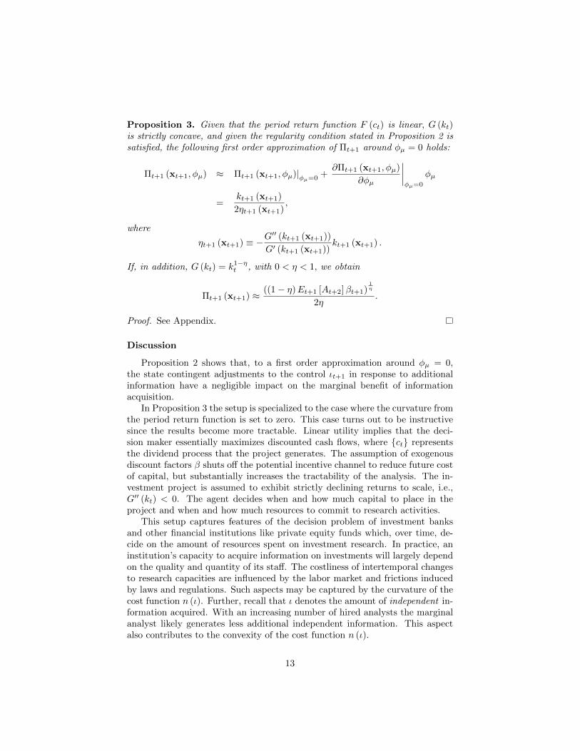
Proposition 3. Given that the period return function F (ct) is linear, G (kt)is strictly concave, and given the regularity condition stated in Proposition 2 issatisfied, the following first order approximation of Πt+1 around φµ = 0 holds:

Πt+1 (xt+1, φµ) ≈ Πt+1 (xt+1, φµ)|φµ=0 +∂Πt+1 (xt+1, φµ)

∂φµ

∣∣∣∣φµ=0

φµ

=kt+1 (xt+1)

2ηt+1 (xt+1),

where

ηt+1 (xt+1) ≡ −G′′ (kt+1 (xt+1))

G′ (kt+1 (xt+1))kt+1 (xt+1) .

If, in addition, G (kt) = k1−ηt , with 0 < η < 1, we obtain

Πt+1 (xt+1) ≈ ((1− η)Et+1 [At+2]βt+1)1η

2η.

Proof. See Appendix.

Discussion

Proposition 2 shows that, to a first order approximation around φµ = 0,the state contingent adjustments to the control ιt+1 in response to additionalinformation have a negligible impact on the marginal benefit of informationacquisition.

In Proposition 3 the setup is specialized to the case where the curvature fromthe period return function is set to zero. This case turns out to be instructivesince the results become more tractable. Linear utility implies that the deci-sion maker essentially maximizes discounted cash flows, where ct representsthe dividend process that the project generates. The assumption of exogenousdiscount factors β shuts off the potential incentive channel to reduce future costof capital, but substantially increases the tractability of the analysis. The in-vestment project is assumed to exhibit strictly declining returns to scale, i.e.,G′′ (kt) < 0. The agent decides when and how much capital to place in theproject and when and how much resources to commit to research activities.

This setup captures features of the decision problem of investment banksand other financial institutions like private equity funds which, over time, de-cide on the amount of resources spent on investment research. In practice, aninstitution’s capacity to acquire information on investments will largely dependon the quality and quantity of its staff. The costliness of intertemporal changesto research capacities are influenced by the labor market and frictions inducedby laws and regulations. Such aspects may be captured by the curvature of thecost function n (ι). Further, recall that ι denotes the amount of independent in-formation acquired. With an increasing number of hired analysts the marginalanalyst likely generates less additional independent information. This aspectalso contributes to the convexity of the cost function n (ι).

13

Proposition 3 indicates that the marginal benefit Πt+1 is not level indepen-dent. It depends on the scale of investment kt+1. This paper considers thecase of stationary productivity. In the case of growth, adjustments to the in-formation acquisition technology would have to capture the increasing cost ofobtaining comparable information levels for larger projects.

Uncertainty reduction yields a more precise conditional productivity esti-mate in each future state. This in turn allows sharper variations in the deci-sions in reaction to different estimates in the various future states of the world.For example, in the state of a high conditional productivity estimate, moreprecision might encourage the decision maker to reduce consumption more infavor of investment. Yet, curvature on the production function, as character-ized by the elasticity ηt, which diminishes the variability of investment, reducesthe marginal benefit of information acquisition. The elasticity scales down thebenefit since it reduces the decision maker’s flexibility to adjust future controlsin response to different signals in different states of the world. The followingcomparative statics summarize the results from Proposition 3.

Comparative Statics (in Ref. to Proposition 3) The benefit of informa-tion acquisition is higher in times

1. when productivity is expected to be high

2. when discount factors are high (less discounting)

3. when the scalability of investments is high

4. when technology changes are expected to have a persistent impact on pro-ductivity.

The simulations of the model presented below mirror these results. Theplots displayed in Figure I show changes in average information acquisition asinduced by changes in different exogenous parameters of the model. Details ofthe simulation are given in the description below Figure I.

Higher marginal cost of information acquisition, as influenced by the pa-rameter χ, decrease information acquisition. A higher value of η decreases thescalability of investment and thus reduces information acquisition ι. High per-sistence in productivity, as captured by the parameter φµ, increases the futurevalue of information about the current state of productivity and therefore en-courages information acquisition. The parameter ωz changes the unconditionallevel of technology risk σ2

µ : higher exogenous risk exposures increase the in-centive to obtain information (Note that due to the exponential specification ofσ2µ the case of ωz = 0 does not correspond to the absence of technology risk.).

Finally, the parameter ωa varies the unconditional productivity level: higherproductivity increases capital investment k and thus the incentive to acquireinformation.

14

0.5 1 1.5

-60

-40

-20

0

20

40

Marginal Info. Acqu. Cost

χ

∆%InformationAcq.ι

0.8 0.85 0.9 0.95

-8

-6

-4

-2

0

2Discount Factor

β

∆%InformationAcq.ι

0.2 0.4 0.6 0.8

0

50

100

Economies of Scale

η

∆%InformationAcq.ι

0.2 0.4 0.6 0.8

-50

0

50

100Persistence of Productivity

φμ∆%InformationAcq.ι

0 0.1 0.2 0.3 0.40

20

40

Technology Risk Exposure

ωz

∆%InformationAcq.ι

0.1 0.2 0.3 0.4 0.5

-10

0

10Mean Log-Productivity

ωa

∆%InformationAcq.ι

Figure 2: The plots show percentage changes in average information acquisitionι, relative to the level under the base parameter setup listed below. Variation iscaused by changes in the exogenous parameters indicated on the horizontal axes.All other parameters are fixed at their base levels. An exception is the plot thatconsiders variation in η: Here the parameter ωa is adjusted simultaneously tokeep the deterministic steady state output level fixed. Without this adjustmentthe effect goes in the same direction and is even more pronounced. The plotsare based on a stochastic simulation of the model under the assumptions madein proposition 3. A second order Taylor approximation of the decision andtransition functions of the model are computed. The method uses a perturbation

15

FIGURE I: The plots show percentage changes in average information acqui-sition ι, relative to the level under the base parameter setup listed in Table1. Variation is caused by changes in the exogenous parameters indicated onthe horizontal axes. All other parameters are fixed at their base levels. Anexception is the plot that considers variation in η: here the parameter ωa is ad-justed simultaneously to keep the deterministic steady state output level fixed.Without this adjustment the effect goes in the same direction and is even morepronounced. The plots are based on a stochastic simulation of the model underthe assumptions made in Proposition 3. A second order Taylor approximationof the decision and transition functions of the model are computed. The methoduses a perturbation approach (Judd [35]) for computing the quadratic approxi-mation of the policy function. The base parameter setup for the simulations isprovided in Table I.

15

Base Parameter Setup

φµ 0.5000 β 0.9500

η 0.5000 σz 0.3000

ωa 0.3722 σv 0.0500

χ 0.0050 φz 0.6000

κ 4.0000 ωz 0.0000

ϕσ 0.0030

Simulated Mean Values

Y 1.0866 a 0.3780

c 0.5683 s 0.0016

k 0.5162 µ 0.0033

ι 0.6109 σ2µ 0.0038

σ2 0.0094 z 0.0059

Table 1: The table lists the base parameters and simulated mean values ofendogenous variables from the solution (see additional details in the caption ofFigure I).

Interpretation of the Years Pre and Post 2000/2001

The results may shed some light on the substantial employment fluctua-tions at major investment banks observed in the years pre and post 2000/2001.Traditionally, especially Anglo-Saxon investment houses have a reputation forsubstantial employment fluctuations. In 1996, for example, headcount at Gold-man Sachs was 6000; by 2001, it was 23,000 and by 2003 it was down to 19,500.Merrill Lynch increased the number of employees from 46,000 in 1995 to 72,000in 2000, and then made 24,000 redundancies globally in two years from mid2001 to mid 2003. As shown in Figure II, these examples were no exceptions —other top investment banks saw similar employment fluctuations.

16

1996 1997 1998 1999 2000 2001 2002 2003 2004 2005 2006-1

0

1

2

3

4

5

6

7

8

9

10

Year

Changeinthenumberofemployeesrelativetothelevelin1996 Employment Fluctuations at Major Investment Banks

Citigroup Global Mkts Hl

Credit Suisse USA Inc

Goldman Sachs Group Inc

Lehman Brothers Holdings Inc

Merrill Lynch

Morgan Stanley

Figure 1: Employment fluctuations at major investment banks. This figureplots changes in the number of employees at major investment banks relativeto their level in 1996. ¥

In the late 1990s conditional productivity estimates were presumably good.Investors were likely to expect that the new internet technologies would havea persistent impact on future productivity, making them a valuable object tolearn about. At the same time, according to the analysis, low expected returnswould have further increased the incentive to acquire information.In contrast, post 2000/2001, productivity forecasts were revised downwards

markedly (compare figure 6 in Pastor and Veronesi [36] on profitability). Mar-kets exhibited low liquidity which increased the cost of adjusting investmentlevels in reaction to information. Further, accounting scandals were essentiallydeteriorating the financial system’s information acquisition technology; they ef-fectively increased the cost of information acquisition faced by investors. Thecheap signal from financial records turned out to be noisier than previouslythought. Finally, risk prices increased quite substantially.Overall, these ’stylized facts’ seem to match the predictions on the dynamic

links between information acquisition and the asset market fairly well. Labor isa costly overhead for financial institutions, frictions to changing the size of thework force may be quite substantial. The results suggests that hiring and firing

17

FIGURE II: Employment fluctuations at major investment banks. This figureplots changes in the number of employees at major investment banks relativeto their level in 1996.

In the late 1990s conditional productivity estimates were presumably good.Investors were likely to expect that the new internet technologies would havea persistent impact on future productivity, making them a valuable object tolearn about. At the same time, according to the analysis, low expected returnswould have further increased the incentive to acquire information.

In contrast, post 2000/2001, productivity forecasts were revised downwardsmarkedly (compare Figure 6 in Pastor and Veronesi [36] on profitability). Mar-kets exhibited low liquidity which increased the cost of adjusting investmentlevels in reaction to information. Further, accounting scandals were essentiallydeteriorating the financial system’s information acquisition technology; they ef-fectively increased the cost of information acquisition faced by investors. Thecheap signal from financial records turned out to be noisier than previouslythought. Finally, risk prices increased quite substantially.

Overall, these stylized facts seem to match the predictions on the dynamiclinks between information acquisition and the asset market fairly well. Labor isa costly overhead for financial institutions, frictions to changing the size of thework force may be quite substantial. The results suggests that hiring and firing

17

decisions by the financial sector might be an interesting signal of the institutions’conditional expectations on productivity, expected returns, and liquidity.

Long Term Investments, Financial Constraints, and Liquidity

The model also sheds some light on the fact that private equity funds andhedge funds benefit more from investment research if clients commit capital fora longer time horizon. Long-term capital commitments reduce outside restric-tions on the funds’ intertemporal investment allocation and thus increase thevalue of marginal knowledge. The results also suggest that private equity funds’information acquisition on start-ups is more valuable when liquid IPO markets,high productivity, and low cost of capital are anticipated in the future.

Generally, restrictions on future investment decisions as for example imposedby required cash outflows are predicted to decrease an institution’s investmentsin information: it binds the intertemporal investment policy and diminishesthe flexibility to respond to marginal information. Firms that are financiallyconstrained and thus face limitations to the scalability of their investments arelikely to invest less in research on the productivity of available projects.

2.6 Human Capital and Information Acquisition

In this Section I consider a slightly adjusted setup where the agent has somehuman capital or skill to acquire information. The level of skill is subject todepreciation and there are adjustment cost. The level of human capital will bedenoted by h. To ensure tractability, the hidden productivity state µt is nowassumed to be independently distributed over time such that signals have valuein exactly one period. This setup is convenient since it will allow us to write themarginal return on information acquisition in terms of known functions of con-sumption, information acquisition, and the level of human capital, without theneed for an approximation. Similar to before, we consider an affine specificationfor at+1:

at+1 = ωa,t + µt + σaεa,t+1. (19)

Notice that there is a slight twist in the timing relative to the setup used so far:at+1 is now a function of µt, not of µt+1. Since the signal structure will be leftunchanged (as in equation (7)) this timing change is necessary for the signalto have value under the assumption that µt is independently distributed overtime. Specifically, µt is now assumed to be normal with zero mean and varianceσ2µ,t−1, where, as before σ2

µ,t−1, is specified as a function of the Markov statezt−1:

µt = σ2µ,t−1εµ,t (20)

To allow for persistent changes in conditional expectations about productivityωa,t is now assumed to follow a stationary Markov process:

ωa,t+1 = ω + φωωa,t + σωεω,r+1. (21)

18

In this Section, skill to acquire information is determined by past informationacquisition activity. This assumption is motivated by the notion of learning onthe job: the more information the agent acquired in the past the more proficientshe has become, and the fewer resources she needs to exert to acquire newinformation today. To capture this notion in the simplest form, the level ofhuman capital ht will be set equal to last period’s information acquisition levelιt, depreciated by a factor δh that accounts for the speed with which this typeof human capital becomes obsolescent, i.e., it characterizes the persistence inskill:

ht = δhιt−1 with 0 ≤ δh < 1. (22)

For simplicity, I consider a quadratic information acquisition cost function7

that features the notion that higher levels of human capital ht allow the agentto acquire information at lower cost:

n (ιt, ht) = χ(ιt − ht)2

2with χ > 0. (23)

The budget constraint is now given by

Yt = kt + n (ιt, ht) + ct. (24)

The level of human capital ht and the conditional log productivity parameterωa,t yield two additional state variables. The state may thus be summarized by

the vector xt =(yt, ht, ωa,t, µt, σ

2t , zt

)′. The corresponding state vector transi-

tion equations are given by:

yt+1 = at+1 + log G (kt)ht+1 = δhιtωa,t+1 = ω + φωωa,t + σωεω,r+1

µt+1 =σ2µ

σ2µ+

σ2vιt

st+1

σ2t+1 =

σ2µ,t

1+σ2µ,t

σ2vιt

zt+1 = ωz + φzzt + σzεz,t+1

(25)

Proposition 4. The decision problem associated with the Bellman equation(13) adjusted by the specifications given in equations (19) to (25) implies thefollowing necessary intertemporal condition for optimal information acquisitionι :

Et

[mt+1

Πt+1 + δt+1MCt+1

(σ2t+2

)MCt

(σ2t+1

) ]= 1,

7The results do not hinge on this specific functional form. More generally, the results holdfor any strictly increasing, weakly convex function n (ι, h), with ∂n (ι, h) /∂ι|ι=0 ≤ 0 for h ≥ 0.Merely for the purpose of simplifying the final expression, Proposition 4 also uses the specialrelation ∂n (ι, h) /∂ι = −∂n (ι, h) /∂h that holds under this quadratic functional specification(see Appendix).

19

where mt+1 = βtF′(ct+1)

F ′(ct)denotes the stochastic discount factor, and

Πt+1 =1

2

(st+1

σ2µ,t

G (kt+1)

G′ (kt+1)− Covt+1 [at+2,mt+2Yt+2]

V art+1 [at+2]

)MCt

(σ2t+1

)= −nι (ιt, ht)

/∂σ2

t+1

(σ2µ,t, ιt

)∂ιt

δt+1 = δh∂σ2

t+2

(σ2µ,t+1, ιt+1

)∂ιt+1

/∂σ2

t+1

(σ2µ,t, ιt

)∂ιt

∂σ2t+1

(σ2µ,t, ιt

)∂ιt

= −σ2µ,t

σ2µ,t

σ2v

(1 + ιt

σ2µ,t

σ2v

)−2

Under linear utility with exogenous, discount factors β, and G (kt) = k1−η with0 < η < 1, the following equation holds

Et

[Πγ=0t+1

]= Et

[kt+1

2η

]= Et

[((1− η)βEt+1 [At+2])

1η

2η

]

=((1− η)β)

1η e

1ηω+φωωa,t+

12 (σ2

t+1+σ2v)+ 1

2η (σ2ω+σ4

µ,t/V art[st+1])

2η

Proof. See Appendix.

The structure of the optimality condition in Proposition 4 is similar to theones presented in the previous Propositions 1 and 3. In particular, for thecase of linear utility, the formula provided for Et [Πt+1] is identical to the onegiven in Proposition 3. The benefit of the setup considered in Proposition 4is that the results do not hinge on the approximation assumptions made underPropositions 2 and 3. This is due to the fact that persistence in skill, as modeledin this Section, provides a more tractable intertemporal link than persistence inthe hidden productivity state.

It is worth noting that given ωa,t and σ2µ,t are time invariant (i.e., under

i.i.d. productivity) there is a constant optimal steady state level for ι that isimplicitly determined by the provided optimality condition.

Limitations and Policy Implications

The framework remains agnostic with respect to the relative importanceof the various economic forces that determine the parameters of the informa-tion acquisition technology. Which economic factors drive the level of marginalcost and which have an impact on the intertemporal scalability of information

20

acquisition? Which transition policies would be required to alter information ac-quisition technologies of a financial system and how costly are these transitions?These questions call for a more explicit analysis of micro-economic informationstructures and are not addressed by this paper. They are subject of an im-portant literature that explicitly studies different market and intermediationstructures.

Yet, the framework may give guidance on the properties of an informationacquisition technology that are of relevance. For example, low persistence inthe process that governs technology risk exposures of an economy increasesthe relative value of flexibility enhancing policies, such as reductions of labormarket rigidities. In a cost-benefit analysis of different system reform policiesthe framework might help identifying the relative benefits from altering differentchannels of a financial system that influence information acquisition.

3 Conclusion

In this paper I examine the link between optimal information acquisitionand conditional expectations on future asset market dynamics. The presentedmodel predicts that investors that are Bayesian learners acquire more informa-tion in times when future capital productivity is expected to be high, expectedreturns are low, new technologies are expected to have a persistent impact onproductivity, and future investment scalability is expected to be high. Economicmechanisms that decrease the scalability of investment diminish the marginalgains from information acquisition since they restrict the flexibility to respondto news.

References

[1] L. Pastor, P. Veronesi, Rational ipo waves, Journal of Finance 60 (4) (2005)p1713 – 1757.

[2] L. P. Hansen, Beliefs, doubts and learning: Valuing macroeconomic risk,American Economic Review 97 (2) (2007) 1–30.

[3] L. P. Hansen, T. J. Sargent, J. Tallarini, Thomas D, Robust permanentincome and pricing, Review of Economic Studies 66 (4) (1999) 873–907.

[4] L. P. Hansen, T. J. Sargent, Robust control and model uncertainty, Amer-ican Economic Review 91 (2) (2001) 60–66.

[5] L. P. Hansen, T. J. Sargent, Robust control of forward-looking models,Journal of Monetary Economics 50 (3) (2003) 581–604.

[6] L. P. Hansen, T. J. Sargent, N. E. Wang, Robust permanent income andpricing with filtering, Macroeconomic Dynamics 6 (1) (2002) 40–84.

21

[7] L. Pastor, P. Veronesi, Stock valuation and learning about profitability,The Journal of Finance 58 (5) (2003) 1749–1789.

[8] J. Lewellen, J. Shanken, Learning, asset-pricing tests, and market efficiency,Journal of Finance 57 (3) (2002) 1113–1145.

[9] T. Adrian, F. Franzoni, Learning about beta: Time-varying factor loadings,expected returns, and the conditional CAPM, Journal of Empirical Finance16 (4) (2009) 537–556.

[10] S. J. Grossman, J. E. Stiglitz, On the impossibility of informationally effi-cient markets, American Economic Review 70 (3) (1980) 393–408.

[11] R. E. Verrecchia, Information acquisition in a noisy rational expectationseconomy, Econometrica 50 (6) (1982) 1415–30.

[12] G. Barlevy, P. Veronesi, Information acquisition in financial markets, Re-view of Economic Studies 67 (1) (2000) 79–90.

[13] J. Peress, Wealth, information acquisition, and portfolio choice, Review ofFinancial Studies 17 (3) (2004) 879–914.

[14] L. L. Veldkamp, Information markets and the comovement of asset prices,Review of Economic Studies 73 (3) (2006) 823–845.

[15] J. Wang, A model of intertemporal asset prices under asymmetric informa-tion, Review of Economic Studies 60 (2) (1993) 249–82.

[16] C. A. Sims, Stickiness, Carnegie-Rochester Conference Series on PublicPolicy 49 (1998) 317–356.

[17] C. A. Sims, Implications of rational inattention, Journal of Monetary Eco-nomics 50 (3) (2003) 665–690.

[18] Y. Luo, Consumption dynamics, asset pricing, and welfare effects underinformation processing constraints, 2005 Meeting Papers 345, Society forEconomic Dynamics (2005).

[19] G. Turmuhambetova, Decision making in an economy with endogenousinformation, Phd dissertation, The University of Chicago (2005).

[20] C. A. Sims, Rational inattention: a research agenda, Discussionpaper, Princeton University, Department of Economics, available athttp://sims.princeton.edu/yftp/RIplus/RatInattPlus.pdf (Mar. 2006).

[21] A. B. Abel, J. C. Eberly, S. Panageas, Optimal inattention to the stockmarket with information costs and transactions costs, Econometrica 81 (4)(2013) 1455–1481.

[22] V. Ng, R. F. Engle, M. Rothschild, A multi-dynamic-factor model for stockreturns, Journal of Econometrics 52 (1-2) (1992) 245–266.

22

[23] D. B. Nelson, Conditional heteroskedasticity in asset returns: A new ap-proach, Econometrica 59 (2) (1991) 347–70.

[24] D. W. Diamond, Financial intermediation and delegated monitoring, Re-view of Economic Studies 51 (3) (1984) 393–414.

[25] R. M. Townsend, Optimal contracts and competitive markets with costlystate verification, Journal of Economic Theory 21 (2) (1979) 265–293.

[26] R. L. Porta, F. L. de Silanes, A. Shleifer, R. W. Vishny, Law and finance,Journal of Political Economy 106 (6) (1998) 1113–1155.

[27] G. D’Avolio, E. Gildor, A. Shleifer, Technology, information production,and market efficiency, Harvard Institute of Economic Research WorkingPapers 1929, Harvard - Institute of Economic Research (2001).

[28] A. Dyck, A. Morse, L. Zingales, Who Blows the Whistle on CorporateFraud?, Journal of Finance 65 (6) (2010) 2213–2253.

[29] D. W. Diamond, R. E. Verrecchia, Information aggregation in a noisy ra-tional expectations economy, Journal of Financial Economics 9 (3) (1981)221–235.

[30] M. F. Hellwig, On the aggregation of information in competitive markets,Journal of Economic Theory 22 (3) (1980) 477–498.

[31] A. R. Admati, A noisy rational expectations equilibrium for multi-assetsecurities markets, Econometrica 53 (3) (1985) 629–57.

[32] A. R. Admati, P. Pfleiderer, A monopolistic market for information, Jour-nal of Economic Theory 39 (2) (1986) 400–438.

[33] A. R. Admati, P. Pfleiderer, Viable allocations of information in financialmarkets, Journal of Economic Theory 43 (1) (1987) 76–115.

[34] A. R. Admati, P. Pfleiderer, Selling and trading on information in financialmarkets, American Economic Review 78 (2) (1988) 96–103.

[35] K. L. Judd, Numerical Methods in Economics, The MIT Press, 1998.

[36] L. Pastor, P. Veronesi, Was there a nasdaq bubble in the late 1990s?,Journal of Financial Economics 81 (1) (2006) 61–100.

A Appendix

A.1 Decision Problem

Let kt be risky investment, ct consumption, ιt learning-effort, and Ft thedecision maker’s information set at time t which includes the history of signals

23

denoted by (at, st) ≡ (at, st) , (at−1, st−1) , (at−2, st−2) , · · · . The productiontechnology is given by

Yt+1 = At+1Gt (kt)

where Yt+1 denotes output at time t+1, Gt is a strictly increasing, concave, andFt-measurable function, and At+1 is stochastic conditional on Ft and furtherspecified below.

Let βt ∈ (0, 1) be a discount factor and F (ct+j) a strictly increasing and con-cave one-period utility function, and yt ≡ log Yt. Given observed initial values(y0, µ0, σ

2p,0, z0

)and an initial value of the hidden state µ0 that is unobserved

by the decision maker, we consider the sequential problem to maximize

F (ct) + Et

∞∑j=1

(j−1∏i=0

βt+i

)F (ct+j) (26)

subject to

ct = Yt − kt − nt (ιt)

yt+1 = at+1 + logGt (kt)

at+1 = logAt+1 = ωa,t + µt+1 + σvεa,t+1

st+1 = µt+1 +σv√ιtεs,t+1

µt+1 = ωµ,t + φµµt + σµ,tεµ,t+1, 0 ≤ φµ < 1

µt+1 = ωµ,t + φµσ2v,tµt + σ2

t (at+1 − ωa,t) + σ2t ιtst+1(

σ2t + σ2

t ιt + σ2v,t

)σ2p,t+1 = φ2

µ

σ2t σ

2v,t(

σ2t + σ2

v,t + σ2t ιt)

σ2t = σ2

µ,t + σ2p,t

zt+1 = ωz + φzzt + σzεz,t+1

σ2µ,t = σ2

µ,t (zt) > 0

kt ≥ 0

ιt, Yt > 0

where E [ ·| Ft] denotes the mathematical expectation, given the information setFt, nt (ιt) denotes a Ft−measurable, strictly increasing and convex functionwhich satisfies n′t (ιt)|ιt=0 = 0 for all t, σ2

µ,t (zt) is a Ft−measurable, positive-

valued function of the state zt, and εt = (εa,t, εs,t, εµ,t, εz,t)′

an i.i.d. Gaussianshock process with mean zero and identity covariance matrix. The process µtis not observed by the decision maker. Associated with this problem is theBellman equation

V (xt) = maxut=(kt,ιt)

′F (ct) + βtE [V (xt+1) |Ft] (27)

24

with the state vector xt ≡(yt, µt, σ

2p,t, zt

)′, the vector of controls ut≡ (kt, ιt)

′,

and where V (xt) denotes the optimal value of the objective function startingfrom state xt. The state vector transition equations xt+1 = h (xt,ut, at+1, st+1, εz,t+1)may be written as follows:

yt+1 = at+1 + logGt (kt)

µt+1 = φµat+1−ωa,t+ιtst+1+

σ2vσ2tµt

1+ιt+σ2vσ2t

σ2p,t+1 = φ2

µσ2v

1+ιt+σ2vσ2t

zt+1 = ωz + φzzt + σzεz,t+1

The first-order necessary conditions for the problem on the right side of equation(27) is

∫∂x′t+1

∂ut

∂V (xt+1)

∂xt+1fa,s,εz (at+1, st+1, εz,t+1|xt,ut) dλ (at+1, st+1, εz,t+1) +∫

V (xt+1)∂fa,s,εz (at+1, st+1, εz,t+1|xt,ut)

∂utdλ (at+1, st+1, εz,t+1)

=F ′ (ct)

βt

(1

n′t (ιt)

)with Lebesgue measure λ and fa,s,εz (at+1, st+1, εz,t+1|Ft) denoting the jointconditional probability density function of the vector (at+1, st+1, εz,t+1)

′. Note

that due to the given independence assumptions one may write

∂fa,s,εz (at+1, st+1, εz,t+1|xt,ut)∂ut

=

(0

∂fa,s(at+1,st+1|xt,ut)∂ιt

)· fεz (εz,t+1|Ft) .

Further,

∂x′t+1

∂ut=

∂h (xt,ut, at+1, st+1, εz,t+1)′

∂ut

=

G′t(kt)Gt(kt)

0 0 0

0 ∂µt+1

∂ιt

∂σ2p,t+1

∂ιt0

Euler Equation

By the envelope theorem one obtains

∂V (xt)

∂yt= F ′ (ct) · Yt

25

which yields the familiar Euler equation

βtE

[G′t (kt)

Gt (kt)

∂V ′ (xt+1)

∂yt+1

∣∣∣∣Ft] = F ′ (ct)

βtE [At+1G′t (kt)F

′ (ct+1)| Ft] = F ′ (ct)

A.2 Basic Formulas

This section gives the derivation of some basic formulas that are used in thederivation of the first-order necessary condition for ιt.

Kalman Filter

The hidden state µt+1 evolves according to the stationary Markov process

µt+1 = ωµ,t + φµµt + σµ,tεµ,t+1,

the signals are given by(at+1

st+1

)=

(ωa,t

0

)+ µt+1 · 1 +

(σv,t 00

σv,t√ιt

)(εa,t+1

εs,t+1

),

where 1 denotes a 2×1 vector of ones, (εa,t, εµ,t, εs,t)′is an i.i.d. Gaussian shock

process with mean zero and identity covariance matrix, and ιt > 0. Define thenotation

σ2t ≡ V ar [µt+1|Ft]µt ≡ E [µt+1|Ft]

where Ft denotes the information set at time t which contains the history ofsignals (at, st). Further let N

(µ0, σ

20

)be the initial distribution of µ. The

conditional moments(µt, σ

2t

)are given by the recursion

µt = ωµ,t−1 + φµσ2v,t−1µt−1 + σ2

t−1 (at − ωa,t−1) + σ2t−1ιt−1st(

σ2t−1 + σ2

t−1ιt−1 + σ2v,t−1

)σ2t = σ2

µ,t + φ2µ

σ2t−1σ

2v,t−1(

σ2t−1 + σ2

v,t−1 + σ2t−1ιt−1

) .

26

Some Useful Derivatives

∂µt+1

(at+1, st+1, µt, σ

2t , ιt

)∂ιt

=

∂

ωµ,t + φµ

σ2v,tµt+σ

2t (at+1−ωa,t)+σ2

t ιtst+1

(σ2t+σ2

t ιt+σ2v,t)

∂ιt

= φµσ2t

(σ2v,t + σ2

t

)(st+1 − µt)− σ2

t (at+1 − ωa,t − µt)(σ2t + σ2

t ιt + σ2v,t

)2∂ ∂µt+1

∂ιt

∂at+1= − φµσ

4t(

σ2t + σ2

t ιt + σ2v,t

)2∂ ∂µt+1

∂ιt

∂st+1=

φµσ2t

(σ2v,t + σ2

t

)(σ2t + σ2

t ιt + σ2v,t

)2∂µt+1

(at+1, st+1, µt, σ

2t , ιt

)∂µt

=

∂

ωµ,t + φµ

σ2v,tµt+σ

2t (at+1−ωa,t)+σ2

t ιtst+1

(σ2t+σ2

t ιt+σ2v,t)

∂µt

= φµσ2v,t

σ2t + σ2

t ιt + σ2v,t

∂µt+1

(at+1, st+1, µt, σ

2t , ιt

)∂σ2

t

=

∂

ωµ,t + φµ

σ2v,tµt+σ

2t (at+1−ωa,t)+σ2

t ιtst+1

(σ2t+σ2

t ιt+σ2v,t)

∂σ2

t

= φµσ2v,t

(at+1 − (µt + ωa,t)) + ιt (st+1 − µt)(σ2t + σ2

t ιt + σ2v,t

)2∂σ2

t+1

(σ2t , ιt

)∂σ2

t

=

σ2µ,t + φ2

µσ2t−1σ

2v,t−1

(σ2t−1+σ2

v,t−1+σ2t−1ιt−1)

∂σ2

t

= φ2µ

σ4v(

σ2t + σ2

v,t + σ2t ιt)2

27

∂σ2t+1

(σ2t , ιt

)∂ιt

=

σ2µ,t + φ2

µσ2t−1σ

2v,t−1

(σ2t−1+σ2

v,t−1+σ2t−1ιt−1)

∂ιt

= −φ2µ

σ2v,t(

1 + ιt +σ2v,t

σ2t

)2

∂2σ2t+1

(σ2t , ιt

)∂ι2t

= 2φ2µσ

2v,t

(1 + ιt +

σ2v,t

σ2t

)−3

−∂2σ2

t+1

∂ι2t∂σ2

t+1

∂ιt

=2

1 + ιt +σ2v,t

σ2t

A.3 Lemmas

Lemma 1. Let f (at+1, st+1|Ft) denote the conditional joint density of the vec-tor (at+1, st+1)

′. Then the following equality holds:

∂f(at+1,st+1|Ft)∂ιt

f (at+1, st+1|Ft)

= − 1

2σ2v,t

(σ2t + σ2

v,t + ιtσ2t

)2 ·((at+1 − E [at+1|Ft]) σ2

t − (st+1 − E [st+1|Ft])(σ2t + σ2

v,t

))2−V ar

[at+1σ

2t − st+1

(σ2t + σ2

v,t

)|Ft]

Proof. Conditional on Ft the vector (at+1, st+1)′is jointly normal with variance-

covariance matrix:

V ar (at+1, st+1|Ft) =

(σ2t + σ2

v,t σ2t

σ2t σ2

t +σ2v,t

ιt

)with

det [V ar (at+1, st+1|Ft)]

=σ2v,t

ιt

(σ2t + σ2

v,t + σ2t ιt)

and

V ar (at+1, st+1|Ft)−1=

ιtσ2v,t

(σ2t +

σ2v,t

ιt−σ2

t

−σ2t σt + σ2

v,t

)(σ2t + ιtσ2

t + σ2v,t

) .

28

Define

∂f(at+1,st+1|Ft)∂ιt

f (at+1, st+1|Ft)

=

∂∂ιt

expΥ2π det[V ar(at+1,st+1|Ft)]0.5

f (at+1, st+1|Ft)

where the following definition applies:

Υ(at+1, st+1, ιt, σ

2t , µt

)≡ −1

2

(at+1 − E [at+1|Ft]st+1 − E [st+1|Ft]

)′V ar (at+1, st+1|Ft)−1 ·(

at+1 − E [at+1|Ft]st+1 − E [st+1|Ft]

)= − 1

2σ2v,t

(σ2t + ιtσ2

t + σ2v,t

) ·(ιtσ

2t + σ2

v,t

)(at+1 − E [at+1|Ft])2

+

ιt(σ2t + σ2

v,t

)(st+1 − E [st+1|Ft])2 −

2σ2t ιt (at+1 − E [at+1|Ft]) (st+1 − E [st+1|Ft])

.

To determine∂f(at+1,st+1|Ft)

∂ιt

f(at+1,st+1|Ft) , consider the derivative

∂Υ(at+1, st+1, ιt, σ

2t , µt

)∂ιt

= −1

2

(σ2t (at+1 − E [at+1|Ft])−

(σ2t + σ2

v,t

)(st+1 − E [st+1|Ft])

)2σ2v,t

(σ2t + ιtσ2

t + σ2v,t

)2Note that

1

2

σ2t + σ2

v,t

ιt(σ2t + σ2

v,t + σ2t ιt)

=1

2

V ar[at+1σ

2t − st+1

(σ2t + σ2

v,t

)|Ft]

σ2v,t

(σ2t + σ2

v,t + σ2t ιt)2

where

V ar[at+1σ

2t − st+1

(σ2t + σ2

v,t

)|Ft]

= σ4t

(σ2t + σ2

v,t

)+(σ2t + σ2

v,t

)2(σ2t +

σ2v,t

ιt

)− 2σ4

t

(σ2t + σ2

v,t

)= σ2

v,t

(σ2t + σ2

v,t

)( σ2t

ιt+σ2v,t

ιt+ σ2

t

)

29

In addition, one may write

1

2π det [V ar (at+1, st+1|Ft)]0.5

=1

2π

(σ2v,t

(σ2t + σ2

v,t + σ2t ιt)

ιt

)−0.5

Taking the derivative w.r.t. ιt yields

∂

∂ιt

1

2π det [V ar (at+1, st+1|Ft)]0.5

=∂

∂ιt

1

2π

(σ2v,t

(σ2t + σ2

v,t + σ2t ιt)

ιt

)−0.5

=

σ2t+σ2

v,t

2ιt(σ2t+σ2

v,t+σ2t ιt)

2π det [V ar (at+1, st+1|Ft)]0.5

=

V ar[at+1σ2t−st+1(σ2

t+σ2v,t)|Ft]

2σ2v,t(σ2

t+σ2v,t+σ

2t ιt)

2

2π det [V ar (at+1, st+1|Ft)]0.5

Taking these results together yields the stated relation.

Lemma 2.

∂f(at+1,st+1|Ft)∂µt

f (at+1, st+1|Ft)=

(at+1 − µt − ωa,t) + ιt (st+1 − µt)σ2t + σ2

v,t + ιtσ2t

.

Proof. To determine∂f(at+1,st+1|Ft)

∂µt

f(at+1,st+1|Ft) consider the derivative

∂Υ(at+1, st+1, ιt, σ

2t , µt

)∂µt

=(at+1 − µt − ωa,t) + ιt (st+1 − µt)

σ2t + σ2

v,t + ιtσ2t

The result directly follows.

Lemma 3.

∂f(at+1,st+1|Ft)∂σ2

p,t

f (at+1, st+1|Ft)

=1

2

((at+1 − E [at+1|Ft]) + ιt (st+1 − E [st+1|Ft]))2(σ2t + ιtσ2

t + σ2v,t

)2 −

1

2

V ar [at+1 + ιtst+1|Ft](σ2t + σ2

v,t + σ2t ιt)2

30

Proof. Consider the derivative

∂Υ(at+1, st+1, ιt, σ

2t , µt

)∂σ2

p,t

=1

2

((at+1 − E [at+1|Ft]) + ιt (st+1 − E [st+1|Ft]))2(σ2t + ιtσ2

t + σ2v,t

)2and

∂

∂σ2p,t

1

2π det [V ar (at+1, st+1|Ft)]0.5

=∂

∂σ2t

1

2π

(σ2v,t

(σ2t + σ2

v,t + σ2t ιt)

ιt

)− 12

=

1

2π

(σ2v,t

(σ2t + σ2

v,t + σ2t ιt)

ιt

)− 12 (−1

2

)(1 + ιt)(

σ2t + σ2

v,t + σ2t ιt)

=− 1

2(1+ιt)

(σ2t+σ2

v,t+σ2t ιt)

2π det [V ar (at+1, st+1|Ft)]0.5

=

− 12

(1+ιt)(σ2t+σ2

v,t+σ2t ιt)

(σ2t+σ2

v,t+σ2t ιt)

2

2π det [V ar (at+1, st+1|Ft)]0.5

Thus, one may verify the result

∂f(at+1,st+1|Ft)∂σ2

p,t

f (at+1, st+1|Ft)

=1

2

((at+1 − E [at+1|Ft]) + ιt (st+1 − E [st+1|Ft]))2(σ2t + ιtσ2

t + σ2v,t

)2 −

1

2

(1 + ιt)(σ2t + σ2

v,t + σ2t ιt)(

σ2t + σ2

v,t + σ2t ιt)2

where(1 + ιt)

(σ2t + σ2

v,t + ιtσ2t

)= V ar [at+1 + ιtst+1|Ft] .

The following Lemmas make use of the following condition and definitions:

Condition 1. The function Ω (x) satisfies the following conditions

1. Ω (x) is a function of the state vector x only,2. Ω (h (a, s, εz)) is everywhere differentiable,

3. Et

[∣∣∣∂h′(a,s,εz)∂(a,s,εz)′

∂Ω(x)∂x

∣∣∣] <∞.31

Definitions

ζ∂yt,t+1 ≡ (at+1 − st+1 − ωa,t)σ2v,t

ζ∂µt,t+1 ≡(σ2t + σ2

v,t

)(st+1 − Et [st+1])− σ2

t (at+1 − Et [at+1])

φµσ2t σ

2v,t

ζ∂µ2

t,t+1 ≡((at+1 − Et [at+1]) σ2

t − (st+1 − Et [st+1])(σ2t + σ2

v,t

))2φ2µσ

4t σ

4v,t

−

V art[at+1σ

2t − st+1

(σ2t + σ2

v,t

)]φ2µσ

4t σ

4v,t

It may be verified that

Et

[ζ∂yt,t+1

]= Et

[ζ∂µt,t+1

]= Et

[ζ∂µ

2

t,t+1

]= 0

and

Covt

[ζ∂µt,t+1, (at+1, st+1, εz,t+1)

′]

=

0σ2t ιt+σ

2t+σ2

v,t

φµιtσ2t

0

′

Covt

[ζ∂yt,t+1, (at+1, st+1, εz,t+1)

′]

=

1− 1ιt

0

′

Lemma 4. Let Ω be a function that satisfies condition (1) then

E

[∂Ω (xt+1)

∂yt+1

∣∣∣∣Ft] = E[ζ∂yt,t+1Ω (xt+1)

∣∣∣Ft] .Proof. Since ζ∂yt,t+1 and the vector (at+1, st+1, εz,t+1)

′are jointly normal condi-

tional on Ft one may write by the multivariate version of Stein’s Lemma

E

[(at+1 − st+1 − ωa,t)

σ2v,t

Ω (xt+1)

∣∣∣∣Ft]

=

1− 1ιt

0

′ ∂x′t+1

∂ (at+1, st+1, εz,t+1)′E

[∂Ω (xt+1)

∂xt+1

∣∣∣∣Ft]

= E

[∂Ω (xt+1)

∂yt+1

∣∣∣∣Ft]where

∂x′t+1

∂ (at+1, st+1, εz,t+1)′ =

1

φµσ2t

σ2t+σ2

t ιt+σ2v,t

0 0

0φµσ

2t ιt

σ2t+σ2

t ιt+σ2v,t

0 0

0 0 0 σz

. (28)

32

Lemma 5. Let Ω be a function that satisfies condition (1) then

E[ζ∂µt,t+1Ω (xt+1)

∣∣∣Ft] = E

[∂Ω (xt+1)

∂µt+1

∣∣∣∣Ft]Proof. By the multivariate version of Stein’s Lemma

E[ζ∂µt,t+1Ω (xt+1)

∣∣∣Ft]= Cov

[ζ∂µt,t+1,Ω (xt+1)

∣∣∣Ft]=

0σ2t+σ2

t ιt+σ2v,t

φµσ2t ιt

0

′

∂x′t+1

∂ (at+1, st+1, εz,t+1)′E

[∂Ω (xt+1)

∂xt+1

∣∣∣∣Ft]

= E

[∂Ω (xt+1)

∂µt+1

∣∣∣∣Ft]

Lemma 6. Let Ω be a function that satisfies condition (1) then

E [ (at+1 − E [at+1|Ft]) Ω (xt+1)| Ft]

=(σ2t + σ2

v,t

)E

[∂Ω (xt+1)

∂yt+1

∣∣∣∣Ft]+ φµσ2tE

[∂Ω (xt+1)

∂µt+1

∣∣∣∣Ft]Proof. By the multivariate version of Stein’s Lemma one may write

E [ (at+1 − E [at+1|Ft]) Ω (xt+1)| Ft]

=

σ2t + σ2

v,t

σ2t

0

′ ∂x′t+1

∂ (at+1, st+1, εz,t+1)E

[∂Ω (xt+1)

∂xt+1

∣∣∣∣Ft]

=(σ2t + σ2

v,t

)E

[∂Ω (xt+1)

∂yt+1

∣∣∣∣Ft]+ φµσ2tE

[∂Ω (xt+1)

∂µt+1

∣∣∣∣Ft]

Lemma 7. Let Ω be a function that satisfies condition (1) then

E [ (st+1 − E [st+1|Ft]) Ω (xt+1)| Ft]

= σ2tE

[∂Ω (xt+1)

∂yt+1

∣∣∣∣Ft]+ φµσ2tE

[∂Ω (xt+1)

∂µt+1

∣∣∣∣Ft]Proof. By the multivariate version of Stein’s Lemma one may write

E [ (st+1 − E [st+1|Ft]) Ω (xt+1)| Ft]

=

σ2t

σ2t +

σ2v,t

ιt0

′

∂x′t+1

∂ (at+1, st+1, εz,t+1)E

[∂Ω (xt+1)

∂xt+1

∣∣∣∣Ft]

= σ2tE

[∂Ω (xt+1)

∂yt+1

∣∣∣∣Ft]+ φµσ2tE

[∂Ω (xt+1)

∂µt+1

∣∣∣∣Ft]

33

Lemma 8. Let Ω be a function that satisfies condition (1) then

Et

[ζ∂µ

2

t,t+1Ω (xt+1)]

= Et

[∂2Ω (xt+1)

∂µ2t+1

](29)

Proof. Since ζ∂µ2

t,t+1 is not conditionally jointly normal with the vector (at+1, st+1, εz,t+1)′

consider the decomposition((at+1 − Et [at+1]) σ2

t − (st+1 − Et [st+1])(σ2t + σ2

v,t

))2=

((at+1 − Et [at+1])(st+1 − Et [st+1])

)′·( (

σ2t

)2(at+1 − Et [at+1])− σ2

t

(σ2t + σ2

v,t

)(st+1 − Et [st+1])(

σ2t + σ2

v,t

)2(st+1 − Et [st+1])− σ2

t

(σ2t + σ2

v,t

)(at+1 − Et [at+1])

)Then, one may write

Et

[V (xt+1)

((at+1 − Et [at+1]) σ2

t − (st+1 − Et [st+1])(σ2t + σ2

v,t

))2]= Covt

[(σ2t

)2at+1 − σ2

t

(σ2t + σ2

v,t

)st+1,Ω (xt+1) (at+1 − Et [at+1])

]+

Covt

[(σ2t + σ2

v,t

)2st+1 − σ2

t

(σ2t + σ2

v,t

)at+1,Ω (xt+1) (st+1 − Et [st+1])

]First, consider

Covt

[(σ2t

)2at+1 − σ2

t

(σ2t + σ2

v,t

)st+1,Ω (xt+1) (at+1 − Et [at+1])

]= Covt

[(σ2t

)2at+1 − σ2

t

(σ2t + σ2

v,t

)st+1, (at+1, st+1, εz,t+1)

′]·

Et

[∂x′t+1

∂ (at+1, st+1, εz,t+1)′∂Ω (xt+1)

∂xt+1(at+1 − Et [at+1])

]+

Covt

[(σ2t

)2at+1 − σ2

t

(σ2t + σ2

v,t

)st+1, (at+1, st+1, εz,t+1)

′]·

Et

[∂ (at+1 − E [at+1|Ft])∂ (at+1, st+1, εz,t+1)

′ Ω (xt+1)

]Substituting

Covt

[(σ2t

)2at+1 − σ2

t

(σ2t + σ2

v,t

)st+1, (at+1, st+1, εz,t+1)

′]

=

0

− σ2tσ

2v,t(σ

2t+σ2

v,t+σ2t ιt)

ιt0

′

and rearranging yields

Covt

[(σ2t

)2at+1 − σ2

t

(σ2t + σ2

v,t

)st+1,Ω (xt+1) (at+1 − Et [at+1])

]= −φµσ2

v,tσ4tEt

[∂Ω (xt+1)

∂µt+1(at+1 − Et [at+1])

]

34

Given that ∂Ω(xt+1)∂µt+1

satisfies condition (1) one may write by Lemma (6)

Et

[∂Ω (xt+1)

∂µt+1(at+1 − Et [at+1])

]=

(σ2t + σ2

v,t

)Et

[∂2Ω (xt+1)

∂yt+1∂µt+1

]+ φµσ

2tEt

[∂2Ω (xt+1)

∂µ2t+1

]which yields

Covt

[(σ2t

)2at+1 − σ2

t

(σ2t + σ2

v,t

)st+1,Ω (xt+1) (at+1 − Et [at+1])

]= −φµσ2

v,tσ4t

(σ2t + σ2

v,t

)Et

[∂2Ω (xt+1)

∂yt+1∂µt+1

]−

φ2µσ

2v,tσ

6tEt

[∂2Ω (xt+1)

∂µ2t+1

]

Next, consider the term

Covt

[(σ2t + σ2

v,t

)2st+1 − σ2

t

(σ2t + σ2

v,t

)at+1,Ω (xt+1) (st+1 − Et [st+1])

]= Covt

[(σ2t + σ2

v,t

)2st+1 − σ2

t

(σ2t + σ2

v,t

)at+1, (at+1, st+1, εz,t+1)

′]·

Et

[∂x′t+1

∂ (at+1, st+1, εz,t+1)′∂Ω (xt+1)

∂xt+1(st+1 − Et [st+1])

]+

Covt

[(σ2t + σ2

v,t

)2st+1 − σ2

t

(σ2t + σ2

v,t

)at+1, (at+1, st+1, εz,t+1)

′]·

Et

[∂ (st+1 − Et [st+1])

∂ (at+1, st+1, εz,t+1)′Ω (xt+1)

]Substituting

Covt

[(σ2t + σ2

v,t

)2st+1 − σ2

t

(σ2t + σ2

v,t

)at+1, (at+1, st+1, εz,t+1)

′]

=

0σ2v,t(σ

2t+σ2

v,t)(σ2t+σ2

v,t+ιtσ2t )

ιt0

′

and rearranging yields

Covt

[(σ2t + σ2

v,t

)2st+1 − σ2

t

(σ2t + σ2

v,t

)at+1,Ω (xt+1) (st+1 − Et [st+1])

]=

σ2v,t

(σ2t + σ2

v,t

) (σ2t + σ2

v,t + ιtσ2t

)ιt

·(φµσ

2t ιt

σ2t + σ2

t ιt + σ2v,t

Et

[∂Ω (xt+1)

∂µt+1(st+1 − Et [st+1])

]+ Et [Ω (xt+1)]

)

35

Given that ∂Ω(xt+1)∂µt+1

satisfies condition (1) one may write by Lemma (7)

Et

[∂Ω (xt+1)

∂µt+1(st+1 − Et [st+1])

]= σ2

tEt

[∂2Ω (xt+1)

∂yt+1∂µt+1

]+ φµσ

2tEt

[∂2Ω (xt+1)

∂µ2t+1

]which yields

Covt

[(σ2t + σ2

v,t

)2st+1 − σ2

t

(σ2t + σ2

v,t

)at+1,Ω (xt+1) (st+1 − Et [st+1])

]= φµσ

2v,t

(σ2t + σ2

v,t

)σ4tEt

[∂2Ω (xt+1)

∂yt+1∂µt+1

]+

φ2µσ

2v,t

(σ2t + σ2

v,t

)σ4tEt

[∂2Ω (xt+1)

∂µ2t+1

]+

σ2v,t

(σ2t + σ2

v,t

) (σ2t + σ2

v,t + ιtσ2t

)ιt

Et [Ω (xt+1)]

Substituting these results yields

Et

[Ω (xt+1)

((at+1 − Et [at+1]) σ2

t − (st+1 − Et [st+1])(σ2t + σ2

v,t

))2]= φ2

µσ4t σ

4v,tEt

[∂2Ω (xt+1)

∂µ2t+1

]+

V art[at+1σ

2t − st+1

(σ2t + σ2

v,t

)]· Et [Ω (xt+1)]

since

V art[at+1σ

2t − st+1

(σ2t + σ2

v,t

)]=

σ2v,t ·

(σ2t + σ2

v,t

)·(ιtσ

2t + σ2

t + σ2v,t

)ιt

.

Thus, one obtains

Et

[ζ∂µ

2

t,t+1Ω (xt+1)]

=Et

[((at+1 − Et [at+1]) σ2

t − (st+1 − Et [st+1])(σ2t + σ2

v,t

))2Ω (xt+1)

]φ2µσ

4t σ

4v,t

−

V art[at+1σ

2t − st+1

(σ2t + σ2

v,t

)]φ2µσ

4t σ

4v,t

Et [Ω (xt+1)]

= Et

[∂2Ω (xt+1)

∂µ2t+1

]

36

Lemma 9. Given the value function V (xt+1) satisfies condition (1) the follow-ing equality holds:

E

[V (xt+1)

∂f(at+1,st+1|Ft)∂µt

f (at+1, st+1|Ft)

∣∣∣∣∣Ft]

= E

[∂V (xt+1)

∂yt+1

∣∣∣∣Ft]+(1 + ιt) σ

2t

σ2t + σ2

v,t + ιtσ2t

φµE

[∂V (xt+1)

∂µt+1

∣∣∣∣Ft]

Proof. Using the previously derived representation of∂f(at+1,st+1|Ft)

∂µt

f(at+1,st+1|Ft) one maywrite

E

[V (xt+1)

∂f(at+1,st+1|Ft)∂µt

f (at+1, st+1|Ft)

∣∣∣∣∣Ft]

=Et [V (xt+1) (at+1 − Et [at+1|])] + ιtEt [V (xt+1) (st+1 − µt)]

σ2t + σ2

v,t + ιtσ2t

Given that V (xt+1) satisfies condition (1) one may write by Lemma (6) andLemma (7) :

E [ (at+1 − E [at+1|Ft])V (xt+1)| Ft]=

(σ2t + σ2

v,t

)E[∂V (xt+1)∂yt+1

∣∣∣Ft]+ φµσ2tE[∂V (xt+1)∂µt+1

∣∣∣Ft]E [ (st+1 − E [st+1|Ft])V (xt+1)| Ft]

= σ2tE[∂V (xt+1)∂yt+1

∣∣∣Ft]+ φµσ2tE[∂V (xt+1)∂µt+1

∣∣∣Ft]Substituting these results and gathering common terms yields

E

[V (xt+1)

∂f(at+1,st+1|Ft)∂µt

f (at+1, st+1|Ft)

∣∣∣∣∣Ft]

= E

[∂V (xt+1)

∂yt+1

∣∣∣∣Ft]+(1 + ιt) σ

2t

σ2t + σ2

v,t + ιtσ2t

φµE

[∂V (xt+1)

∂µt+1

∣∣∣∣Ft]

Lemma 10. The shadow value of µ has the following recursive representation:

∂V (xt)

∂µt= βtE

[∂V (xt+1)

∂yt+1

∣∣∣∣Ft]+ φµβtE

[∂V (xt+1)

∂µt+1

∣∣∣∣Ft]

37

Proof. By the envelope theorem one may write ∂V (xt)∂µt

as follows

∂V (xt)

∂µt

= βtE

[∂h′t+1

∂µt

∂V (xt+1)

∂xt+1+ V (xt+1)

∂f(at+1,st+1|Ft)∂µt

f (at+1, st+1|Ft)

∣∣∣∣∣Ft]

= βtE

[∂µt+1

∂µt

∂V (xt+1)

∂µt+1+ V (xt+1)

∂f(at+1,st+1|Ft)∂µt

f (at+1, st+1|Ft)

∣∣∣∣∣Ft]

since

∂h′t+1

∂µt=

0

∂µt+1

∂µt

00

′

where∂f(at+1,st+1|xt,ut)

∂µt

f (at+1, st+1|xt,ut)=

(at+1 − µt − ωa,t) + ιt (st+1 − µt)σ2t + σ2

v,t + ιtσ2t

as defined and derived above. Since, as shown above, ∂µt+1

∂µtis Ft−measurable

one may further write

∂V (xt)

∂µt(30)

= βt∂µt+1

∂µtE

[∂V (xt+1)

∂µt+1

∣∣∣∣Ft]+ βtE

[V (xt+1)

∂f(at+1,st+1|Ft)∂µt

f (at+1, st+1|Ft)

∣∣∣∣∣Ft]

Further, using Lemma (9) and the previously derived representation for ∂µt+1

∂µt,

∂µt+1

∂µt= φµ

σ2v,t

σ2t + σ2

t ιt + σ2v,t

,

one may write equation (30) as follows

∂V (xt)

∂µt= βtφµ

σ2v,t

σ2t + σ2

t ιt + σ2v,t

E

[∂V (xt+1)

∂µt+1

∣∣∣∣Ft]+

βtE

[∂V (xt+1)

∂yt+1

∣∣∣∣Ft]+

βtφµσ2t + σ2

t ιtσ2t + σ2

t ιt + σ2v,t

E

[∂V (xt+1)

∂µt+1

∣∣∣∣Ft]This yields

∂V (xt)

∂µt= βtE

[∂V (xt+1)

∂yt+1

∣∣∣∣Ft]+ φµβtE

[∂V (xt+1)

∂µt+1

∣∣∣∣Ft] . (31)

38

Lemma 11.

E

[∂µt+1

∂ιt

∂V (xt+1)

∂µt+1|Ft]

= −∂σ2

p,t+1

∂ιtE

[∂2V (xt+1)

∂µ2t+1

|Ft]. (32)

Proof. Note that given the previous definitions one may write

∂µt+1

∂ιt= −

∂σ2p,t+1

∂ιt· ζ∂µt,t+1.

Given that ∂V (xt+1)∂µt+1

satisfies condition (1) , one directly obtains the stated result

by applying Lemma (5) .

Lemma 12. Define V RS (xt,u (xt)) as the right side of equation (27) evaluated

at the optimal policy function u (xt). ∂2V (xt+1)∂µ2

t+1has the following representation:

∂2V (xt+1)

∂µ2t+1

= βt+1E

[∂2V (xt+2)

∂y2t+2

∣∣∣∣Ft+1

]+ (33)

φ2µβt+1E

[∂2V (xt+2)

∂µ2t+2

∣∣∣∣Ft+1

]+

2φµβt+1E

[∂2V (xt+2)

∂yt+2∂µt+2

∣∣∣∣Ft+1

]+

2∂2V RS (xt+1,u (xt+1))

∂µt+1∂u (xt+1)

∂u (xt+1)

∂µt+1+

∂2V RS (xt+1,u (xt+1))

∂2u (xt+1)

(∂u (xt+1)

∂µt+1

)2

.

Proof. Moving equation (31) one period forward and differentiating w.r.t. µt+1

yields

∂2V (xt+1)

∂µ2t+1

=∂2V RS (xt+1,u (xt+1))

∂µ2t+1

+ 2∂2V RS (xt+1,u (xt+1))

∂µt+1∂u (xt+1)

∂u (xt+1)

∂µt+1+

∂2V RS (xt+1,u (xt+1))

∂2u (xt+1)

(∂u (xt+1)

∂µt+1

)2

By differentiating (31) w.r.t. µt+1 one obtains

∂2V RS (xt+1,u (xt+1))

∂µ2t+1

= βt+1

∂E[∂V (xt+2)∂yt+2

∣∣∣Ft+1

]∂µt+1

+φµβt+1

∂E[∂V (xt+2)∂µt+2

∣∣∣Ft+1

]∂µt+1

(34)First, consider the term

∂E[∂V (xt+2)∂yt+2

∣∣∣Ft+1

]∂µt+1

(35)

= E

∂ ∂V (xt+2)∂yt+2

∂µt+1

∣∣∣∣∣∣Ft+1

+ E

∂V (xt+2)

∂yt+2

∂f(at+2,st+2|xt+1,ut+1)∂µt+1

f (at+2, st+2|xt+1,ut+1)

∣∣∣∣∣∣Ft+1

39

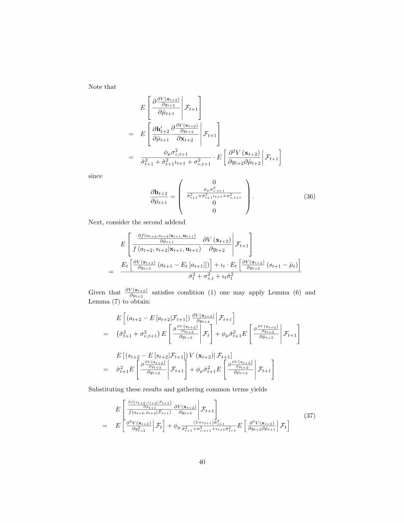
Note that

E

∂ ∂V (xt+2)∂yt+2

∂µt+1

∣∣∣∣∣∣Ft+1

= E

∂h′t+2

∂µt+1

∂ ∂V (xt+2)∂yt+2

∂xt+2

∣∣∣∣∣∣Ft+1

=

φµσ2v,t+1

σ2t+1 + σ2

t+1ιt+1 + σ2v,t+1

· E[∂2V (xt+2)

∂yt+2∂µt+2

∣∣∣∣Ft+1

]since

∂ht+2

∂µt+1=

0

φµσ2v,t+1

σ2t+1+σ2

t+1ιt+1+σ2v,t+1

00

. (36)

Next, consider the second addend

E

∂f(at+2,st+2|xt+1,ut+1)∂µt+1

f (at+2, st+2|xt+1,ut+1)

∂V (xt+2)

∂yt+2

∣∣∣∣∣∣Ft+1

=

Et

[∂V (xt+2)∂yt+2

(at+1 − Et [at+1|])]

+ ιt · Et[∂V (xt+2)∂yt+2

(st+1 − µt)]

σ2t + σ2

v,t + ιtσ2t

Given that ∂V (xt+2)∂yt+2

satisfies condition (1) one may apply Lemma (6) and

Lemma (7) to obtain:

E[

(at+2 − E [at+2|Ft+1]) ∂V (xt+2)∂yt+2

∣∣∣Ft+1

]=

(σ2t+1 + σ2

v,t+1

)E

[∂∂V (xt+2)∂yt+2

∂yt+2

∣∣∣∣∣Ft]

+ φµσ2t+1E

[∂∂V (xt+2)∂yt+2

∂µt+2

∣∣∣∣∣Ft+1

]

E [ (st+2 − E [st+2|Ft+1])V (xt+2)| Ft+1]

= σ2t+1E

[∂∂V (xt+2)∂yt+2

∂yt+2

∣∣∣∣∣Ft+1

]+ φµσ

2t+1E

[∂∂V (xt+2)∂yt+2

∂µt+2

∣∣∣∣∣Ft+1

]

Substituting these results and gathering common terms yields

E

[∂f(at+2,st+2|Ft+1)

∂µt+1

f(at+2,st+2|Ft+1)∂V (xt+2)∂yt+2

∣∣∣∣∣Ft+1

]= E

[∂2V (xt+2)∂y2t+2

∣∣∣Ft]+ φµ(1+ιt+1)σ2

t+1

σ2t+1+σ2

v,t+1+ιt+1σ2t+1

E[∂2V (xt+2)∂yt+2∂µt+1

∣∣∣Ft] (37)

40

Substituting these results into eqn. (35) and gathering common terms yields

∂E[∂V (xt+2)∂yt+2

∣∣∣Ft+1

]∂µt+1

(38)

= E

[∂2V (xt+2)

∂y2t+2

∣∣∣∣Ft+1

]+ φµE

[∂2V (xt+2)

∂yt+2∂µt+2

∣∣∣∣Ft+1

]Next, consider the term

∂E[∂V (xt+2)∂µt+2

∣∣∣Ft+1

]∂µt+1

= E

∂ ∂V (xt+2)∂µt+2

∂µt+1

∣∣∣∣∣∣Ft+1

+ E

∂V (xt+2)

∂µt+2

∂f(at+2,st+2|Ft+1)∂µt+1

f (at+2, st+2|Ft+1)

∣∣∣∣∣∣Ft+1

where, using (36), the first addend may be written as follows

E

∂ ∂V (xt+2)∂µt+2

∂µt+1

∣∣∣∣∣∣Ft+1

= E

∂h′t+2

∂µt+1

∂ ∂V (xt+2)∂µt+2

∂xt+2

∣∣∣∣∣∣Ft+1

=

φµσ2v,t+1

σ2t+1 + σ2

t+1ιt+1 + σ2v,t+1

E

[∂2V (xt+2)

∂µ2t+2

∣∣∣∣Ft+1

]Further, analogous to (37) , one may write the second addend by Lemma (6)and Lemma (7) as follows:

E

[∂f(at+2,st+2|Ft+1)

∂µt+1

f(at+2,st+2|Ft+1)∂V (xt+2)∂µt+2

∣∣∣∣∣Ft+1

]

= E

[∂∂V (xt+2)∂µt+2

∂yt+2

∣∣∣∣∣Ft+1

]+ φµ

(1+ιt+1)σ2t+1

σ2t+1+σ2

v,t+1+σ2t+1ιt+1

E[∂2V (xt+2)∂µ2

t+2

∣∣∣Ft+1

]Substituting the results for the two addends yields

dE[∂V (xt+2)∂µt+2

∣∣∣Ft+1

]dµt+1

(39)

= E

∂ ∂V (xt+2)∂µt+2

∂yt+2

∣∣∣∣∣∣+ φµE

[∂2V (xt+2)

∂µ2t+2

∣∣∣∣Ft+1

]

41

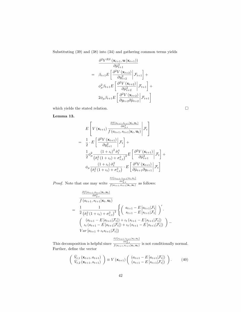
Substituting (39) and (38) into (34) and gathering common terms yields

∂2V RS (xt+1,u (xt+1))

∂µ2t+1

= βt+1E

[∂2V (xt+2)

∂y2t+2

∣∣∣∣Ft+1

]+

φ2µβt+1E

[∂2V (xt+2)

∂µ2t+2

∣∣∣∣Ft+1

]+

2φµβt+1E

[∂2V (xt+2)

∂yt+2∂µt+2

∣∣∣∣Ft+1

]which yields the stated relation.

Lemma 13.

E

V (xt+1)

∂f(at+1,st+1|xt,ut)∂σ2

p,t

f (at+1, st+1|xt,ut)

∣∣∣∣∣∣Ft

=1

2· E[∂2V (xt+1)

∂y2t+1

∣∣∣∣Ft]+

1

2φ2µ

(1 + ιt)2σ4t(

σ2t (1 + ιt) + σ2

v,t

)2E [ ∂2V (xt+1)

∂µ2t+1

∣∣∣∣Ft]+

φµ(1 + ιt) σ

2t(

σ2t (1 + ιt) + σ2

v,t

) · E [ ∂2V (xt+1)

∂µt+1∂yt+1

∣∣∣∣Ft]

Proof. Note that one may write

∂f(at+1,st+1|xt,ut)∂σ2p,t

f(at+1,st+1|xt,ut) as follows:

∂f(at+1,st+1|xt,ut)∂σ2

p,t

f (at+1, st+1|xt,ut)

=1

2

1(σ2t (1 + ιt) + σ2

v,t

)2(

at+1 − E [at+1|Ft]st+1 − E [st+1|Ft]

)′·(

(at+1 − E [at+1|Ft]) + ιt (st+1 − E [st+1|Ft])ιt (at+1 − E [at+1|Ft]) + ιt (st+1 − E [st+1|Ft])

)−

V ar [at+1 + ιtst+1|Ft]

This decomposition is helpful since

∂f(at+1,st+1|xt,ut)∂σ2p,t

f(at+1,st+1|xt,ut) is not conditionally normal.

Further, define the vector(Vt,1 (xt+1, at+1)Vt,2 (xt+1, st+1)

)≡ V (xt+1)

((at+1 − E [at+1|Ft])(st+1 − E [st+1|Ft])

). (40)

42

Then one may write

E

V (xt+1)

∂f(at+1,st+1|xt,ut)∂σ2

p,t

f (at+1, st+1|xt,ut)

∣∣∣∣∣∣Ft

=1

2

1(σ2t (1 + ιt) + σ2

v,t

)2 ·Cov

[at+1 + ιtst+1, Vt,1 (xt+1, at+1)

∣∣Ft]+

Cov[ιtat+1 + ιtst+1, Vt,2 (xt+1, st+1)

∣∣Ft]−V ar [at+1 + ιtst+1|Ft]E [V (xt+1)| Ft]

which allows the application of the multivariate version of Stein’s Lemma. First,consider

Cov[at+1 + ιtst+1, Vt,1 (xt+1, at+1)

∣∣Ft]= Cov

[at+1 + ιtst+1, (at+1, st+1, εz,t+1)

′∣∣Ft]E

∂

(xt+1

at+1

)′∂ (at+1, st+1, εz,t+1)

′∂Vt,1 (xt+1, at+1)

∂

(xt+1

at+1

)∣∣∣∣∣∣∣∣∣Ft

where

∂

(xt+1

at+1

)′∂ (at+1, st+1, εz,t+1)

′ =

1

φµσ2t

σ2t+σ2

t ιt+σ2v,t

0 0 1

0φµσ

2t ιt

σ2t+σ2

t ιt+σ2v,t

0 0 0

0 0 0 σz 0

(41)

and

E

∂Vt,1(xt+1,at+1)

∂

xt+1

at+1

∣∣∣∣∣∣∣∣Ft

= E

[(∂V (xt+1)∂xt+1

(at+1 − E [at+1|Ft])V (xt+1)

)∣∣∣∣∣Ft] (42)

andCov

[at+1 + ιtst+1, (at+1, st+1, εz,t+1)

′∣∣Ft]=(σ2t + σ2

v,t + ιtσ2t

) 110

′ . (43)

43

Hence,

Cov[at+1 + ιtst+1, Vt,1 (xt+1, at+1)

∣∣Ft]=

(σ2t + σ2

v,t + ιtσ2t

)·

E

[∂V (xt+1)

∂yt+1(at+1 − E [at+1|Ft])

∣∣∣∣Ft]+ E [V (xt+1)| Ft] +

φµσ2t + σ2

t ιtσ2t + σ2

t ιt + σ2v,t

E

[∂V (xt+1)

∂µt+1(at+1 − E [at+1|Ft])

∣∣∣∣Ft]Further, given that ∂V (xt+1)

∂µt+1satisfies condition (1) one may apply Lemma (6)

to obtain

Cov

[at+1,

∂V (xt+1)

∂µt+1

∣∣∣∣Ft] (44)

=(σ2t + σ2

v,t

)E

[∂2V (xt+1)

∂µt+1∂yt+1

∣∣∣∣Ft]+

φµσ2tE

[∂2V (xt+1)

∂µ2t+1

∣∣∣∣Ft]Substituting this result yields:

Cov[at+1 + ιtst+1, Vt,1 (xt+1, at+1)

∣∣Ft]=

(σ2t + σ2

v,t + ιtσ2t

)·

Cov

[∂V (xt+1)

∂yt+1, at+1

∣∣∣∣Ft]+ E [V (xt+1)| Ft]

+

φµσ2t (1 + ιt) ·

(σ2t + σ2

v,t

)E

[∂2V (xt+1)

∂µt+1∂yt+1

∣∣∣∣Ft]+

φµσ2tE

[∂2V (xt+1)

∂µ2t+1

∣∣∣∣Ft]Next, one may write

Cov[ιtat+1 + ιtst+1, Vt,2 (xt+1, st+1)

∣∣Ft]= Cov

[ιtat+1 + ιtst+1, (at+1, st+1, εz,t+1)

′∣∣Ft] ·E

d

(xt+1

st+1

)′d (at+1, st+1, εz,t+1)

′∂Vt,2 (xt+1, st+1)

∂

(xt+1

st+1

)∣∣∣∣∣∣∣∣∣Ft

Note that

∂

(xt+1

st+1

)′∂ (at+1, st+1, εz,t+1)

′ =

1

φµσ2t

σ2t+σ2

t ιt+σ2v,t

0 0 0

0φµσ

2t ιt

σ2t+σ2

t ιt+σ2v,t

0 0 1

0 0 0 σz 0

(45)

44

and

E

∂Vt,2 (xt+1, st+1)

∂

(xt+1

st+1

)∣∣∣∣∣∣∣∣Ft

= E

[(∂V (xt+1)∂xt+1

(st+1 − E [st+1|Ft])V (xt+1)

)∣∣∣∣∣Ft]

and

Cov[ιtat+1 + ιtst+1, (at+1, st+1, εz,t+1)

′∣∣Ft]= ιt

(σ2t + σ2

v,t + ιtσ2t

)·

110

′

Therefore, one obtains

Cov[ιtat+1 + ιtst+1, Vt,2 (xt+1, st+1)

∣∣Ft]= ιt

(σ2t + σ2

v,t + ιtσ2t

)·

Cov

[∂V (xt+1)

∂yt+1, st+1

∣∣∣∣Ft]+

φµσ2t + σ2

t ιtσ2t + σ2

t ιt + σ2v,t

Cov

[∂V (xt+1)

∂µt+1, st+1

∣∣∣∣Ft]+

E [V (xt+1)| Ft]

Further, given that ∂V (xt+1)∂µt+1

satisfies condition (1) one may apply Lemma (7)

to obtain

Cov

[st+1,

∂V (xt+1)

∂µt+1

∣∣∣∣Ft] (46)

= σ2tE

∂ ∂V (xt+1)∂µt+1

∂yt+1

∣∣∣∣∣∣Ft+ φµσ

2tE

[∂2V (xt+1)

∂µ2t+1

∣∣∣∣Ft]This yields

Cov[ιtat+1 + ιtst+1, Vt,2 (xt+1, st+1)

∣∣Ft]= ιt

(σ2t + σ2

v,t + ιtσ2t

)·

Cov

[∂V (xt+1)

∂yt+1, st+1

∣∣∣∣Ft]+ E [V (xt+1)| Ft]

+

φ2µσ

2t (1 + ιt) σ

2t ιt · E

[∂2V (xt+1)

∂µ2t+1

∣∣∣∣Ft]+

φµσ2t (1 + ιt) σ

2t ιtE

[∂2V (xt+1)

∂µt+1∂yt+1

∣∣∣∣Ft]

45

Substituting the results into,

E

V (xt+1)

∂f(at+1,st+1|xt,ut)∂σ2

p,t

f (at+1, st+1|xt,ut)

∣∣∣∣∣∣Ft

=1

2

1(σ2t (1 + ιt) + σ2

v,t

)2 ·Cov

[at+1 + ιtst+1, Vt,1 (xt+1, at+1)

∣∣Ft]+

Cov[ιtat+1 + ιtst+1, Vt,2 (xt+1, st+1)

∣∣Ft]−V ar [at+1 + ιtst+1|Ft]E [V (xt+1)| Ft]

yields

E

V (xt+1)

∂f(at+1,st+1|xt,ut)∂σ2

p,t

f (at+1, st+1|xt,ut)

∣∣∣∣∣∣Ft

=1

2

1(σ2t (1 + ιt) + σ2

v,t

)2 ·(σ2t + σ2

v,t + ιtσ2t

)Cov

[∂V (xt+1)

∂yt+1, at+1 + ιtst+1

∣∣∣∣Ft]+

(1 + ιt)(σ2t + σ2

v,t + ιtσ2t

)E [V (xt+1)| Ft] +

φµσ2t (1 + ιt)

(σ2t + σ2

v,t + σ2t ιt)E

[∂2V (xt+1)

∂µt+1∂yt+1

∣∣∣∣Ft]+

φ2µσ

4t (1 + ιt)

2E

[∂2V (xt+1)

∂µ2t+1

∣∣∣∣Ft]−V ar [at+1 + ιtst+1|Ft]E [V (xt+1)| Ft]

Finally, given that ∂V (xt+1)∂yt+1

satisfies condition (1) one may apply Lemmas (6)

and (7) to obtain

Cov

[(at+1 + ιtst+1) ,

∂V (xt+1)

∂yt+1

∣∣∣∣Ft]=

(σ2t + σ2

v,t + ιtσ2t

)· E[∂2V (xt+1)

∂y2t+1

∣∣∣∣Ft]+

φµσ2t (1 + ιt)E

[∂2V (xt+1)

∂yt+1∂µt+1

∣∣∣∣Ft]Using this result and

V ar [at+1 + ιtst+1|Ft]= (1 + ιt)

(ιtσ

2t + σ2

v,t + σ2t

),

yields the stated equation.

46

Lemma 14.

E

[∂µt+1 (at+1, st+1|Ft)

∂σ2p,t

∂V (xt+1)

∂µt+1

∣∣∣∣Ft]=

φµσ2v,t(

σ2t + σ2

t ιt + σ2v,t

)E [ ∂2V (xt+1)

∂µt+1∂yt+1

∣∣∣∣Ft]+

φ2µσ

2v,t

(1 + ιt) σ2t(

σ2t + σ2

t ιt + σ2v,t

)2 · E [ ∂2V (xt+1)

∂µ2t+1

∣∣∣∣Ft]Proof. Recall the previously derived formula

∂µt+1

∂σ2p,t

=∂µt+1

∂σ2t

= φµσ2v,t

(at+1 − (µt + ωa,t)) + ιt (st+1 − µt)(σ2t + σ2

t ιt + σ2v,t

)2Thus, one may write

E

[∂µt+1 (at+1, st+1|Ft)

∂σ2p,t

∂V (xt+1)

∂µt+1

∣∣∣∣Ft]=

φµσ2v,t(

σ2t + σ2

t ιt + σ2v,t

)2Cov [at+1 + ιtst+1 ,∂V (xt+1)

∂µt+1

∣∣∣∣Ft]

Given that ∂V (xt+1)∂µt+1

satisfies condition (1) one may apply Lemmas (6) and (7)

to obtain the stated relation.

Lemma 15.

∂V (xt)

∂σ2p,t

(47)

= βtφµE

[∂2V (xt+1)

∂µt+1∂yt+1

∣∣∣∣Ft]+

βtφ2µ (1 + ιt) σ

2t

σ2v,t + 1

2 σ2t (1 + ιt)(

σ2t + σ2

t ιt + σ2v,t

)2E [ ∂2V (xt+1)

∂µ2t+1

∣∣∣∣Ft]+

βt1

2· E[∂2V (xt+1)

∂y2t+1

∣∣∣∣Ft]+

βtE

[∂σ2

p,t+1

∂σ2p,t

∂V (xt+1)

∂σ2p,t+1

∣∣∣∣∣Ft]

47

Proof. By the envelope theorem one may write

∂V (xt)

∂σ2p,t

= βtE

[∂x′t+1

∂σ2p,t

∂V (xt+1)

∂xt+1

∣∣∣∣Ft]+

βtE

V (xt+1)

∂f(at+1,st+1|xt,ut)∂σ2

p,t

f (at+1, st+1|xt,ut)

∣∣∣∣∣∣Ft

= βtE

[∂µt+1

∂σ2p,t

∂V (xt+1)

∂µt+1

∣∣∣∣Ft]+

βtE

[∂σ2

p,t+1

∂σ2p,t

∂V (xt+1)

∂σ2p,t+1

∣∣∣∣∣Ft]

+

βtE

V (xt+1)

∂f(at+1,st+1|xt,ut)∂σ2

p,t

f (at+1, st+1|xt,ut)

∣∣∣∣∣∣Ft

since

βtE

[∂yt+1

∂σ2p,t

∂V (xt+1)

∂yt+1

∣∣∣∣Ft]= βtE

[∂zt+1

∂σ2p,t

∂V (xt+1)

∂zt+1

∣∣∣∣Ft]= 0

where

∂f(at+1,st+1|xt,ut)∂σ2

p,t

f (at+1, st+1|xt,ut)

=1

2

((at+1 − E [at+1|Ft]) + ιt (st+1 − E [st+1|Ft]))2

−V ar [at+1 + ιtst+1|Ft](σ2t + σ2

v,t + ιtσ2t

)2as defined and derived above. Substituting the equations provided by Lemma(14) and (13) and gathering common terms yields the stated equation.

Lemma 16.

Et

[V (xt+1)

∂f(at+1,st+1|Ft)∂ιt

f (at+1, st+1|Ft)

]=

1

2

∂σ2p,t+1

∂ιtEt

[∂2V (xt+1)

∂µ2t+1

](48)

48

Proof. Based on the previous definitions one may write

∂f(at+1,st+1|xt,ut)∂ιt

f (at+1, st+1|xt,ut)

= −1

2φ2µ

σ4t σ

2v,t(

σ2t + σ2

v,t + ιtσ2t

)2 ζ∂µ2

t,t+1

=1

2

∂σ2p,t+1

∂ιtζ∂µ

2

t,t+1.

Applying Lemma (8) directly yields the stated equation.

A.4 Propositions

Proposition 5. The decision problem associated with the Bellman equation (27)implies the following necessary intertemporal condition for optimal informationacquisition ι :

Et

[mt+1

Πt+1 + δt+1MCt+1

(σ2p,t+2

)MCt

(σ2p,t+1

) ]= 1

where mt,t+1 = βtF′(ct+1)

F ′(ct)denotes the stochastic discount factor and the follow-

ing definitions apply

Πt+1 ≡ 1

2

∂2V RS(xt+1,u(xt+1))∂µt+1∂kt+1

∂kt+1(xt+1)∂µt+1

+ ∂2V RS(xt+1,u(xt+1))∂µt+1∂ιt+1

∂ιt+1(xt+1)∂µt+1

F ′ (ct+1)

MCt(σ2p,t+1

)≡ n′t (ιt)

/−∂σ2

p,t+1

(σ2t , ιt

)∂ιt

∂σ2p,t+1

(σ2t , ιt

)∂ιt

≡ −φ2µσ

2v,t(

1 + ιt +σ2v,t

σ2t

)2

δt+1 ≡∂σ2

p,t+2

(σ2t+1, ιt+1

)∂σ2

t+1

=φ2µ(

1 + (1 + ιt+1)σ2t+1

σ2v

)2

and where V RS(xt+1,ut+1

)denotes the right side of the Bellman equation (27)

evaluated at the optimal policy rule u (xt+1).

Proof. Note that the first-order necessary condition for ιt, as derived above,

49

may be written as follows:

E

[∂µt+1

∂ιt

∂V (xt+1)

∂µt+1

∣∣∣∣Ft]+ E

[∂σ2

p,t+1

∂ιt

∂V (xt+1)

∂σ2p,t+1

∣∣∣∣∣Ft]

+ (49)

E

[V (xt+1)

∂f(at+1,st+1|xt,ut)∂ιt

f (at+1, st+1|xt,ut)

∣∣∣∣∣Ft]

=F ′ (ct)n

′t (ιt)

βt

Substituting the previous results (32) and (48) , one obtains

−∂σ2

p,t+1

∂ιtE

[∂2V (xt+1)

∂µ2t+1

∣∣∣∣Ft]+∂σ2

p,t+1

∂ιtE

[∂V (xt+1)

∂σ2p,t+1

∣∣∣∣∣Ft]

+

1

2

∂σ2p,t+1

∂ιtE

[∂2V (xt+1)

∂µ2t+1

∣∣∣∣Ft]=

F ′ (ct)n′t (ιt)

βt

or

E

[∂V (xt+1)

∂σ2p,t+1

∣∣∣∣∣Ft]

=1

2E

[∂2V (xt+1)

∂µ2t+1

∣∣∣∣Ft]+F ′ (ct)n

′t (ιt)

∂σ2p,t+1

∂ιtβt

(50)

Define

θt,σ2p,t≡ 1

2βt · E

[∂2V (xt+1)

∂y2t+1

∣∣∣∣Ft]+

βtφµE

[∂2V (xt+1)

∂µt+1∂yt+1

∣∣∣∣Ft]δt ≡

∂σ2p,t+1

∂σ2p,t

=∂σ2

t+1

∂σ2t

γt,σ2p,t≡ βtφ

2µ (1 + ιt) σ

2t

σ2v,t + 1

2 (1 + ιt) σ2t(

σ2t (1 + ιt) + σ2

v,t

)2such that by (47) ∂V (xt+1)

∂σ2p,t+1

may be written as follows

∂V (xt)

∂σ2p,t

= θt,σ2p,t

+ βtδtE

[∂V (xt+1)

∂σ2p,t+1

∣∣∣∣∣Ft]

+ γt,σ2p,tE

[∂2V (xt+1)

∂µ2t+1

∣∣∣∣Ft] .

50

Substituting (50), rearranging, and going one period forward gives

∂V (xt+1)

∂σ2p,t+1

= θt+1,σ2p,t+1

+ βt+1δt+1F ′ (ct+1)n′t+1 (ιt+1)

βt+1∂σ2

p,t+2

∂ιt+1

+

(γt+1,σ2

p,t+1+

1

2βt+1δt+1

)E

[∂2V (xt+2)

∂µ2t+2

∣∣∣∣Ft+1

]Using the fact that

γt+1,σ2p,t+1

+1

2βt+1δt+1 =

1

2φ2µβt+1

and taking mathematical expectations with respect to Ft yields

E

[∂V (xt+1)

∂σ2p,t+1

∣∣∣∣∣Ft]

(51)

= E[θt+1,σ2

p,t+1

∣∣∣Ft]+ E

βt+1δt+1F ′ (ct+1)n′t+1 (ιt+1)

βt+1∂σ2

p,t+2

∂ιt+1

∣∣∣∣∣∣Ft+

1

2φ2µβt+1E

[∂2V (xt+2)

∂µ2t+2

∣∣∣∣Ft]Substituting (51) into (50) and rearranging yields

E[θt+1,σ2

p,t+1

∣∣∣Ft]+ (52)

E

βt+1δt+1F ′ (ct+1)n′t+1 (ιt+1)

βt+1∂σ2

p,t+2

∂ιt+1

∣∣∣∣∣∣Ft+

1

2φ2µβt+1E

[∂2V (xt+2)

∂µ2t+2

∣∣∣∣Ft]− 1

2E

[∂2V (xt+1)

∂µ2t+1

∣∣∣∣Ft]=

F ′ (ct)n′t (ιt)

βt+1∂σ2

p,t+1

∂ιt

From equation (33) it follows that

1

2E

[φ2µβt+1E

[∂2V (xt+2)

∂µ2t+2

∣∣∣∣Ft+1

]− ∂2V (xt+1)

∂µ2t+1

∣∣∣∣Ft] (53)

= −1

2βt+1E

[E[∂2V (xt+2)∂y2t+2

∣∣∣Ft+1

] ∣∣∣Ft]−βt+1φµE

[E

[∂2V (xt+2)

∂µt+2∂yt+2

∣∣∣∣Ft+1

]∣∣∣∣Ft]−1

2E

[∂2V (xt+1)

∂µ2t+1

− ∂2V RS (xt+1,u (xt+1))

∂µ2t+1

∣∣∣∣Ft]

51

Substituting (53) and the definition of θt+1,σ2p,t+1

into (52) and rearranging yields

the result

E

δt+1

∂σ2p,t+1

∂ιt∂σ2

p,t+2

∂ιt+1

n′t+1 (ιt+1)

n′t (ιt)

βtF′ (ct+1)

F ′ (ct)

∣∣∣∣∣∣Ft+

1

2βtE

∂2V (xt+1)∂µ2

t+1− ∂2V RS(xt+1,u(xt+1))

∂µ2t+1

F ′ (ct)n′t (ιt)/(−∂σ

2p,t+1

∂ιt

)∣∣∣∣∣∣Ft

= 1

where

=∂2V (xt+1)

∂µ2t+1

− ∂2V RS (xt+1,u (xt+1))

∂µ2t+1

= 2∂2V RS (xt+1,u (xt+1))

∂µt+1∂u (xt+1)

∂u (xt+1)

∂µt+1+

∂2V RS (xt+1,u (xt+1))

∂2u (xt+1)

(∂u (xt+1)

∂µt+1

)2

.

First order optimality ensures that

∂V RS (xt+1,u (xt+1))

∂u=

(00

).

Differentiating w.r.t. µt+1 yields

∂V RS (xt+1,u (xt+1))

∂u (xt+1) ∂µt+1+∂2V RS (xt+1,u (xt+1))

∂u2

∂u (xt+1)

∂µt+1= 0

or

∂u (xt+1)

∂µt+1= −

(∂2V RS (xt+1,u (xt+1))

∂u2

)−1∂2V RS (xt+1,u (xt+1))

∂u (xt+1) ∂µt+1.

52

This yields

∂2V (xt+1)

∂µ2t+1

− ∂2V RS (xt+1,u (xt+1))

∂µ2t+1

= 2∂2V RS (xt+1,u (xt+1))

∂µt+1∂u (xt+1)

∂u (xt+1)

∂µt+1

+∂2V RS (xt+1,u (xt+1))

∂2u (xt+1)

(∂u (xt+1)

∂µt+1

)2

=

(∂2V RS (xt+1,u (xt+1))

∂µt+1∂u (xt+1)+∂2V RS (xt+1,u (xt+1))

∂2u (xt+1)

(∂u (xt+1)

∂µt+1

))·

∂u (xt+1)

∂µt+1+∂2V RS (xt+1,u (xt+1))

∂µt+1∂u (xt+1)

∂u (xt+1)

∂µt+1

=∂2V RS (xt+1,u (xt+1))

∂µt+1∂u (xt+1)

∂u (xt+1)

∂µt+1

=∂2V RS

(xt+1,ut+1 (xt+1)

)∂µt+1∂kt+1

∂kt+1 (xt+1)

∂µt+1+∂2V RS (xt+1,u (xt+1))

∂µt+1∂ιt+1

∂ιt+1 (xt+1)

∂µt+1

This yields the final result

Et

[mt,t+1

Πt+1 + δt+1MCt+1

(σ2p,t+2

)MCt

(σ2p,t+1

) ]= 1

where mt,t+1 = βtF′(ct+1)

F ′(ct)denotes the stochastic discount factor and the follow-

ing definitions apply

Πt+1 ≡ 1

2

∂2V RS(xt+1,ut+1)∂µt+1∂kt+1

∂kt+1(xt+1)∂µt+1

+∂2V RS(xt+1,ut+1)

∂µt+1∂ιt+1

∂ιt+1(xt+1)∂µt+1

F ′ (ct+1)

MCt(σ2p,t+1

)≡ n′t (ιt)

/−∂σ2

p,t+1

∂ιt

∂σ2p,t+1

∂ιt≡ −

φ2µσ

2v,t(

1 + ιt +σ2v,t

σ2t

)2

δt+1 ≡∂σ2

t+2

∂σ2t+1

=φ2µ(

1 + (1 + ιt+1)σ2t+1

σ2v

)2

Note that given a well defined problem with a negative definite Hessian(∂2V RS/∂u2

t+1

),

the term Πt+1 is positive state-by-state.

53

Definition 2.

b (xt, φµ)

≡ −σ2v,tβt(

1 + ιt (xt, φµ) +σ2v,t

σ2t

)2

Et∂ ∂V (xt+1(φµ),φµ)

∂σ2p,t+1

− 12∂2V (xt+1(φµ),φµ)

∂µ2t+1

∂yt+1

+

Et

φµ · ∂ ∂V (xt+1(φµ),φµ)

∂σ2p,t+1

− 12∂2V (xt+1(φµ),φµ)

∂µ2t+1

∂µt+1

·∂ιt(xt,φµ)

∂µt

F ′ (ct (xt, φµ))

Condition 3.

|φµb (xt, φµ)||φµ=0 = 0∣∣∣∣φ2µ

∂b (xt, φµ)

∂φµ

∣∣∣∣∣∣∣∣φµ=0

= 0

Proposition 6. The addends that enter the period gain Πt+1 may be writtenas follows:

∂2V RS(xt+1,ut+1)∂µt+1∂kt+1

∂kt+1(xt+1)∂µt+1

F ′ (ct+1)=

Covt+1 [st+2, At+2G′ (kt+1)mt+2]

V art+1 [µt+2]

∂kt+1 (xt+1)

∂µt+1

∂2V RS(xt+1,ut+1)∂µt+1∂ιt+1

∂ιt+1(xt+1)∂µt+1

F ′ (ct+1)= −

φ2µβt+1σ

2v,t+1

F ′ (ct+1)(

1 + ιt+1 +σ2v,t+1

σ2t+1

)2

∂ιt (xt+1)

∂µt+1Et+1

∂ ∂V (xt+2)∂σ2

p,t+2− 1

2∂2V (xt+2)∂µ2

t+2

∂yt+2

+

Et+1

φµ · ∂ ∂V (xt+2)∂σ2

p,t+2− 1

2∂2V (xt+2)∂µ2

t+2

∂µt+2

For small φµ and given condition (3) is satisfied

∂2VRS(xt+1,ut+1)∂µt+1∂ιt+1

∂ιt+1(xt+1)∂µt+1

F ′(ct+1) is to

a first order approximation equal to zero, i.e.

∂2V RS(xt+1,ut+1,φµ)∂µt+1∂ιt+1

∂ιt+1(xt+1,φµ)∂µt+1

F ′ (ct+1 (xt+1, φµ))

≈ φ2µb (xt+1, φµ)

∣∣φµ=0

+dφ2µb (xt+1, φµ)

dφµ

∣∣∣∣∣φµ=0

φµ

= 0.

54

Proposition 7. In the case of a linear period return function the following firstorder approximation of Πt+1 around φµ = 0 holds:

Πt+1 (xt+1, φµ) ≈ Πt+1 (xt+1, φµ)|φµ=0 +∂Πt+1 (xt+1, φµ)

∂φµ

∣∣∣∣φµ=0

φµ

=kt+1 (xt+1)

2ηt+1 (xt+1),

where

ηt+1 (xt+1) ≡ −G′′ (kt+1 (xt+1))

G′ (kt+1 (xt+1))kt+1 (xt+1) .

If, in addition, G (kt) = k1−ηt , with 0 < η < 1, we obtain

Πt+1 ≈((1− η)Et+1 [At+2]βt+1)

1η

2η.

Proof of Propositions 2 & 3. To determine the vector ∂V RS(xt,ut)∂ut∂µt

differentiatethe following vector w.r.t. µt :

∂V RS (xt,ut)

∂ut

= βt

G′t(kt)Gt(kt)

E[∂V ′(xt+1)∂yt+1

∣∣∣Ft]∂σ2

p,t+1

∂ιtE[∂V (xt+1)∂σ2

p,t+1− 1

2∂2V (xt+1)∂µ2

t+1

∣∣∣xt,ut]− F ′ (ct)( 1

n′t (ιt)

)

First, consider the element ∂2V RS(xt,ut)∂kt∂µt

:

∂2V RS (xt,ut)

∂kt∂µt

=∂βtG′t(kt)Gt(kt)

E[∂V ′(xt+1)∂yt+1

∣∣∣Ft]∂µt

= βtG′t (kt)

Gt (kt)

∂E[∂V ′(xt+1)∂yt+1

∣∣∣Ft]∂µt

= βtG′t (kt)

Gt (kt)

(E

[∂2V (xt+1)

∂y2t+1

∣∣∣∣Ft]+ φµE

[∂2V (xt+1)

∂yt+1∂µt+1

∣∣∣∣Ft])which directly follows from equation (38). Further, given that ∂V (xt+1)

∂yt+1satisfies

condition (1) , one may obtain by Lemma (7)

E

[(st+1 − E [st+1|Ft])

σ2t

∂V (xt+1)

∂yt+1

∣∣∣∣Ft]= E

[∂2V (xt+1)

∂y2t+1

∣∣∣∣Ft]+ φµE

[∂2V (xt+1)

∂µt+1∂yt+1

∣∣∣∣Ft]

55

and thus

∂2V RS (xt,ut)

∂kt∂µt

= βtG′t (kt)

Gt (kt)E

[(st+1 − E [st+1|Ft])

σ2t

∂V (xt+1)

∂yt+1

∣∣∣∣Ft]= βt

G′t (kt)

Gt (kt)E

[(st+1 − E [st+1|Ft])

σ2t

At+1Gt (kt)F′ (ct+1)

∣∣∣∣Ft]=

Cov [st+1, At+1G′t (kt)βtF

′ (ct+1)| Ft]σ2t

Next, consider the element ∂2V RS(xt,ut)∂ιt∂µt

:

∂2V RS (xt,ut)

∂ιt∂µt

=∂βt∂σ2

p,t+1

∂ιtE[∂V (xt+1)∂σ2

p,t+1− 1

2∂2V (xt+1)∂µ2

t+1

∣∣∣Ft]∂µt

= βt∂σ2

p,t+1

∂ιt

∂µt+1

∂µtE

[(∂2V (xt+1)

∂σ2p,t+1∂µt+1

− 1

2

∂3V (xt+1)

∂µ3t+1

)∣∣∣∣∣Ft]

+

βt∂σ2

p,t+1

∂ιtE

[(∂V (xt+1)

∂σ2p,t+1

− 1

2

∂2V (xt+1)

∂µ2t+1

) ∂f(at+1,st+1|xt,ut)∂µt

f (at+1, st+1|xt,ut)

∣∣∣∣∣Ft]

= βt∂σ2

p,t+1

∂ιtE

[(∂µt+1

∂µtζ∂µt,t+1 +

∂f(at+1,st+1|xt,ut)∂µt

f (at+1, st+1|xt,ut)

)·(

∂V (xt+1)

∂σ2p,t+1

− 1

2

∂2V (xt+1)

∂µ2t+1

)∣∣∣∣∣Ft]

where the last step follows from Lemma (5) given that ∂2V (xt+1)∂σ2

p,t+1and ∂2V (xt+1)

∂µ2t+1

satisfy

condition (1) . This yields

∂2V RS (xt,ut)

∂ιt∂µt

= βt∂σ2

p,t+1

∂ιtE

[(st+1 − µt)

σ2t

(∂V (xt+1)

∂σ2p,t+1

− 1

2

∂2V (xt+1)

∂µ2t+1

)∣∣∣∣∣Ft]

= βt∂σ2

p,t+1

∂ιt·

E

[∂2V (xt+1)

∂σ2p,t+1∂yt+1

− 1

2

∂3V (xt+1)

∂µ2t+1∂yt+1

∣∣∣∣∣Ft]

+

φµE

[∂2V (xt+1)

∂σ2p,t+1∂µt+1

− 1

2

∂3V (xt+1)

∂µ3t+1

∣∣∣∣∣Ft]

56

where the last step follows from Lemma (7) given that ∂V (xt+1)∂σ2

p,t+1and ∂2V (xt+1)

∂µ2t+1

satisfy

condition (1) . We therefore may summarize the results

∂2V RS(xt,ut)∂µt∂kt

∂kt(xt)∂µt

F ′ (ct)=

Cov [st+1, At+1G′ (kt)mt+1| Ft]

V art [µt+1]

∂kt (xt)

∂µt∂2V RS(xt,ut)

∂µt∂ιt

∂ιt(xt)∂µt

F ′ (ct)= −

φ2µβtσ

2v,t

F ′ (ct)(

1 + ιt +σ2v,t

σ2t

)2

∂ιt (xt)

∂µtE

[∂2V (xt+1)

∂σ2p,t+1∂yt+1

− 1

2

∂3V (xt+1)

∂µ2t+1∂yt+1

∣∣∣∣∣Ft]

+

φµE

[∂2V (xt+1)

∂σ2p,t+1∂µt+1

− 1

2

∂3V (xt+1)

∂µ3t+1

∣∣∣∣∣Ft]

.

Further, given condition (3) is satisfied, we may write a first order approximation

of∂2VRS(xt,ut)

∂µt∂ιt

∂ιt(xt)∂µt

F ′(ct)around φµ = 0 as follows:

∂2V RS(xt,ut,φµ)∂µt∂ιt

∂ιt(xt,φµ)∂µt

F ′ (ct (xt, φµ))

≈φ2µb (xt, φµ)

∣∣φµ=0

+dφ2µb (xt, φµ)

dφµ

∣∣∣∣∣φµ=0

φµ

=φ2µb (xt, φµ)

∣∣φµ=0

+

φ2µ

∂b (xt, φµ)

∂φµ+ 2φµb (xt, φµ)

∣∣∣∣φµ=0

φµ

= 0.

Hence, to a first order approximation of φµ around φµ = 0, the term∂2VRS(xt,ut)

∂µt∂ιt

∂ιt(xt)∂µt

F ′(ct)

is negligible. Further, for a linear period return function, one may write:

Cov [st+1, At+1G′ (kt)mt+1| Ft]

V art [µt+1]

∂kt (xt)

∂µt

=1

2

Cov [st+1, At+1| Ft]V art [µt+1]

G′ (kt)βt∂kt (xt)

∂µt

=1

2

V art [µt+1]

V art [µt+1]Et [At+1]G′ (kt)βt

∂kt (xt)

∂µt

=1

2Et [At+1]G′ (kt)βt

∂kt (xt)

∂µt

=1

2

∂kt (xt)

∂µt

=kt (xt)

2ηt

57

where

ηt ≡ −G′′ (kt)

G′ (kt)kt,

and where we used the fact that by first order optimality the following relationholds,

βtEt [At+1]G′ (kt) = 1,

with

Et [At+1] = exp

ωa + µt +

1

2V art [at+1]

,

and which, by the implicit function theorem, yields the equation

∂kt (xt)

∂µt=ktηt.

Further, for Gt (kt) = k1−η one obtains

kt = ((1− η)Et [At+1]βt)1η

ηt = η

and thus

Πt =((1− η)Et [At+1]βt)

1η

2η.

This completes the proof.

Proposition 8 (Human Capital). The decision problem associated with theBellman equation (27) , adjusted by the specifications

µt = σ2µ,t−1εµ,t

at+1 = ωa,t + µt + σv,tεa,t+1

ωa,t+1 = ω + φωωa,t + σωεω,r+1

ht = δhιt−1 with 0 < δh < 1

n (ιt, ht) = χ(ιt − ht)2

2with χ > 0,

implies the following necessary intertemporal condition for optimal informationacquisition ι :

Et

[mt+1

Πt+1 + δt+1MCt+1

MCt

]= 1

58

where mt+1 = βtF′(ct+1)

F ′(ct)denotes the stochastic discount factor, and

Πt+1 =1

2

(st+1

σ2µ,t

G (kt+1)

G′ (kt+1)− Covt+1 [at+2,mt+2Yt+2]

V art+1 [at+2]

)MCt = −nι (ιt, ht)

/∂σ2

t+1

∂ιt

δt+1 = δh∂σ2

t+2

∂ιt+1

/∂σ2

t+1

∂ιt

∂σ2t+1

∂ιt= −σ2

µ,t

σ2µ,t

σ2v,t

(1 + ιt

σ2µ,t

σ2v

)−2

and where σ2t+1 = σ2

t+1

(σ2µ,t, ιt

). Under log-utility Et

[mt+1Πlog

t+1

]= 0, implying

steady state information acquisition equal to zero (ι = 0). Under linear utilitywith exogenous, Ft−measurable discount factors mt+1 = βt, and G (kt) = k1−η

with 0 < η < 1, the following relation holds

Et

[Πγ=0t+1

]= Et

[((1− η)mt+2Et [At+2])

1η

2η

]

Further, if mt+2 is Ft measurable, we obtain

Et

[Πγ=0t+1

]=

((1− η)mt+2)1η e

1ηω+φωωa,t+

12 (σ2

t+1+σ2v)+ 1

2η (σ2ω+σ4

µ,t/V art[st+1])

2η.

Proof. In this setup, the state is characterized by the vector xt =(yt, ht, µt, σ

2t , zt

)′,

where µt ≡ Et [µt] and σ2t ≡ V art [µt] . The law of motion is given by:

yt+1 = at+1 + logG (kt)ht+1 = δhιt

µt+1 =σ2µ,t

σ2µ,t+

σ2v,tιt

st+1

σ2t+1 =

σ2µ,t

1+σ2µ,t

σ2v,tιt

zt+1 = ωz + φzzt + σzεz,t+1

The first order necessary condition for ιt is given by

F ′ (ct)nι (ιt, ht)

=

∫βt

(∂µt+1

∂ιt

∂V (xt+1)

∂µt+1+∂σ2

p,t+1

∂ιt

∂V (xt+1)

∂σ2t+1

+∂ht+1

∂ιt

∂V (xt+1)

∂ht+1

)·

f (at+1, st+1, εz,t+1|xt,ut) dλ (at+1, st+1, εz,t+1) +∫βtV (xt+1)

∂f (at+1, st+1, εz,t+1|xt,ut)∂ιt

dλ (at+1, st+1, εz,t+1)

59

Since st+1 is independent of (at+1, εz,t+1) one may write

F ′ (ct)nι (ιt, ht)

= Et

[βt

(∂µt+1

∂ιt

∂V (xt+1)

∂µt+1+∂σ2

p,t+1

∂ιt

∂V (xt+1)

∂σ2p,t+1

+∂ht+1

∂ιt

∂V (xt+1)

∂ht+1

)]+

Et

[βtV (xt+1)

∂f(st+1|xt,ut)∂ιt

f (st+1|xt,ut)

]

First, consider the term ∂V (xt+1)∂µt+1

. By the envelope theorem one may write

∂V (xt+1)

∂µt+1=

∂ F (c (xt+1)) + Et+1 [βt+1V (xt+2)]∂µt+1

=∂Et+1 [βt+1V (xt+2)]

∂µt+1

= βt+1

Et+1

∂ft+1(at+2)∂µt+1

ft+1 (at+2)V (xt+2) +

∂V (xt+2)

∂xt+2

∂xt+2

∂µt+1

= βt+1Et+1

∂ft+1(at+2)∂µt+1

ft+1 (at+2)V (xt+2)

It may be verified that

∂ft+1(at+2)∂µt+1

ft+1 (at+2)=at+2 − Et+1 [at+2]

V art+1 [at+2]

with

Et+1 [at+2] = ωa,t+1 + µt+1

V art+1 [at+2] = σ2t+1 + σ2

v

Given V (xt+2) satisfies condition (1) one may write

∂V (xt+1)

∂µt+1= βt+1Covt+1

[at+2 − Et+1 [at+2]

V art+1 [at+2], V (xt+2)

]= βt+1

Covt+1 [at+2, V (xt+2)]

V art+1 [at+2]

= βt+1V art+1 [at+2]

V art+1 [at+2]Et+1

[∂V (xt+2)

∂xt+2

∂xt+2

∂at+2

]= βt+1Et+1

[∂V (xt+2)

∂yt+2

]Further, using the envelope theorem

∂V (xt+2)

∂yt+2= F ′ (ct+2) · Yt+2

60

we obtain

∂V (xt+1)

∂µt+1= βt+1Et+1 [F ′ (ct+2) · Yt+2]

= F ′ (ct+1)G (kt+1)

G′ (kt+1)Et+1

[At+2G

′ (kt+1)βt+1F

′ (ct+2)

F ′ (ct+1)

]∂V (xt+1)

∂µt+1= F ′ (ct+1)

G (kt+1)

G′ (kt+1)

Next, consider the term ∂V (xt+1)∂σ2

t+1. By the envelope theorem we may write

∂V (xt+1)

∂σ2t+1

=∂F (c (xt+1)) + Et+1 [βt+1V (xt+2)]

∂σ2t+1

=∂Et+1 [βt+1V (xt+2)]

∂σ2t+1

= βt+1Et+1

∂ft+1(at+2)∂σ2

t+1

ft+1 (at+2)V (xt+2) +

∂V (xt+2)

∂xt+2

∂xt+2

∂σ2t+1

= βt+1Et+1

∂ft+1(at+2)∂σ2

t+1

ft+1 (at+2)V (xt+2)

It may be verified that

∂ft+1(at+2)∂σ2

t+1

ft+1 (at+2)=

1

2

(at+2 − Et+1 [at+2])2 − V art+1 [at+2]

(V art+1 [at+2])2

Given V (xt+2) satisfies condition (1) we obtain

∂V (xt+1)

∂σ2t+1

= βt+1Et+1

[1

2

(at+2 − Et+1 [at+2])2 − V art+1 [at+2]

(V art+1 [at+2])2 V (xt+2)

]

=βt+1

2

V art+1 [at+2]Et+1

[(at+2 − Et+1 [at+2]) ∂V (xt+2)

∂xt+2

∂xt+2

∂at+2

](V art+1 [at+2])

2

=βt+1

2

Covt+1

[at+2,

∂V (xt+2)∂yt+2

]V art+1 [at+2]

=βt+1

2

Covt+1 [at+2, F′ (ct+2) · Yt+2]

V art+1 [at+2]

=1

2F ′ (ct+1)

G (kt+1)

G′ (kt+1)

Covt+1

[at+2,

βt+1F′(ct+2)

F ′(ct+1) At+2G′ (kt+1)

]V art+1 [at+2]

=1

2F ′ (ct+1)

Covt+1 [at+2,mt+2Yt+2]

V art+1 [at+2]

61

Next, we consider the term ∂V (xt+1)∂ht+1

.

∂V (xt+1)

∂ht+1=

∂F (c (xt+1)) + Et+1 [βt+1V (xt+2)]

∂ht+1

= −F ′ (ct+1)nh (ιt+1, ht+1) +∂Et+1 [βt+1V (xt+2)]

∂ht+1

= −F ′ (ct+1)nh (ιt+1, ht+1) + Et+1

[βt+1

∂V (xt+2)

∂xt+2

∂xt+2

∂ht+1

]= F ′ (ct+1)nι (ιt+1, ht+1)

since, given the functional form assumed, nι (ιt, ht) = −nh (ιt, ht) . Finally con-

sider the term Et

[V (xt+1) ∂ft(st+1)

∂ιt/ft (st+1)

]. It may be verified that

∂ft(st+1)∂ιt

ft (st+1)= −

σ2v,t

2

s2t+1 − V art [st+1](ιtσ2

µ,t + σ2v,t

)2Hence, we obtain

Et

[V (xt+1)

∂ft(st+1)∂ιt

ft (st+1)

]

= −σ2v,t

(Et[s2t+1V (xt+1)

]− V art [st+1]Et [V (xt+1)]

)2(ιtσ2

µ,t + σ2v,t

)2= −

σ2v,t (Covt [st+1, V (xt+1) st+1]− V art [st+1]Et [V (xt+1)])

2(ιtσ2

µ,t + σ2v,t

)2= −

σ2v,tV art [st+1]Et

[∂V (xt+1)∂µt+1

∂µt+1

∂st+1st+1

]2(ιtσ2

µ,t + σ2v,t

)2where

∂µt+1

∂st+1=

σ2µ,t

σ2µ,t +

σ2v,t

ιt

such that

Et

[V (xt+1)

∂ft(st+1)∂ιt

ft (st+1)

]

= −σ2v,tV art [st+1]

σ2µ,t

σ2µ,t+

σ2v,tιt

Et

[∂V (xt+1)∂µt+1

st+1

]2(ιtσ2

µ,t + σ2v,t

)2= −1

2Et

∂V (xt+1)

∂µt+1

st+1σ2µ,t

σ2v,t(

1 + ιtσ2µ,t

σ2v,t

)2

.62

Note that

∂µt+1

∂ιt=

st+1σ2µ,t

σ2v,t(

1 + ιtσ2µ,t

σ2v,t

)2

Hence, we may write

Et

[V (xt+1)

∂ft(st+1)∂ιt

ft (st+1)

]

= −1

2Et

[∂V (xt+1)

∂µt+1

∂µt+1

∂ιt

].

Substituting these results into the FONC yields

1 = Et

mt+1

12

(∂µt+1

∂ιt

G(kt+1)G′(kt+1) +

∂σ2t+1

∂ιt

Covt+1[at+2,mt+2Yt+2]V art+1[at+2]

)+ δhnι (ιt+1, ht+1)

nι (ιt, ht)

where mt+1 ≡ βtF

′(ct+1)F ′(ct)

and

∂µt+1

∂ιt= st+1

σ2µ,t

σ2v,t(

1 + ιtσ2µ,t

σ2v,t

)2

∂σ2t+1

∂ιt= −σ2

µ,t

σ2µ,t

σ2v,t(

1 + ιtσ2µ,t

σ2v,t

)2

In terms of the notation previously used we obtain

Et

[mt+1

Πt+1 + δt+1MCt+1

MCt

]= 1,

with

Πt+1 =1

2

(st+1

σ2µ,t

G (kt+1)

G′ (kt+1)− Covt+1 [at+2,mt+2Yt+2]

V art+1 [at+2]

)MCt = −nι (ιt, ht)

/∂σ2

t+1

∂ιt

δt+1 = δh∂σ2

t+2

∂ιt+1

/∂σ2

t+1

∂ιt

∂σ2t+1

∂ιt= −σ2

µ,t

σ2µ,t

σ2v,t

(1 + ιt

σ2µ,t

σ2v,t

)−2

63

and where σ2t+1 = σ2

t+1

(σ2µ,t, ιt

). Under linear utility with exogenous, Ft mea-

surable discount factors mt+1 = βt,

Covt+1 [at+2,mt+2Yt+2]

= V art+1 [at+2]Et+1 [mt+2At+2]G (kt+1)

The FONC for capital,

Et+1 [mt+2At+2]G′ (kt+1) = 1,

allows us to write

Covt+1 [at+2,mt+2Yt+2]

=G (kt+1)

G′ (kt+1)V art+1 [at+2] .

Substituting this result into the previous equation yields

Πγ=0t+1 =

1

2

G (kt+1)

G′ (kt+1)

(st+1

σ2µ,t

− 1

)=

1

2Et+1 [mt+2At+2]G (kt+1)

(st+1

σ2µ,t

− 1

)where kt+1 is given by

kt+1 = G′−1

(1

Et+1 [mt+2At+2]

)with G′−1 denoting the inverse of G′. For G (kt) = k1−η, with 0 < η < 1 oneobtains

kt+1 = (Et+1 [mt+2At+2] (1− η))1η

G (kt+1) = (Et+1 [mt+2At+2] (1− η))1−ηη

Substituting yields

Πγ=0t+1 =

1

2(1− η)

1−ηη (Et+1 [mt+2At+2])

1η

(st+1

σ2µ,t

− 1

)Taking conditional expectations

Et

[Πγ=0t+1

]=

1

2(1− η)

1−ηη Et

[(Et+1 [mt+2At+2])

1η

(st+1

σ2µ,t

− 1

)]where

Et

[(mt+2Et+1 [At+2])

1η

(st+1

σ2µ,t

− 1

)]Covt

[m

1η

t+2e1ηωa,t+1+µt+1+ 1

2 (σ2t+1+σ2

v,t+1), st+1

]= V ar [s]Et

[m

1η

t+2e1ηωa,t+1+µt+1+ 1

2 (σ2t+1+σ2

v,t+1)]

64

Conditinal on Cov [st+1,mt+2] = 0, such that mt+2 = βt+1 does not reveal anyinformation about the hidden productivity state, we may write

Et

[(mt+2Et+1 [At+2])

1η

(st+1

σ2µ,t

− 1

)]= Et

[m

1η

t+2e1ηωa,t+1+µt+1+ 1

2 (σ2t+1+σ2

v,t+1)(st+1

σ2µ,t

− 1

)]=

1

σ2µ,t

Covt

[m

1η

t+2e1η

ωa,t+1+

∂µt+1∂st+1

st+1+ 12 (σ2

t+1+σ2v,t+1)

, st+1

]−

Et

[m

1η

t+2e1η

ωa,t+1+

∂µt+1∂st+1

st+1+ 12 (σ2

t+1+σ2v,t+1)

]= Et

[m

1η

t+2e1η

ωa,t+1+

∂µt+1∂st+1

st+1+ 12 (σ2

t+1+σ2v,t+1)

](V art [st+1]

σ2µ,t

1

η

∂µt+1

∂st+1− 1

)= Et

[m

1η

t+2e1ηωa,t+1+µt+1+ 1

2 (σ2t+1+σ2

v,t+1)](

1

η− 1

)= Et

[(Et [mt+2At+2])

1η

] 1

η(1− η)

such that

Et

[Πγ=0t+1

]= Et

[((1− η)mt+2Et [At+2])

1η

2η

]which is always greater than zero since since 0 < η < 1. Further, given thatmt+2 is Ft measurable and given that σ2

v,t+1 = σ2v we obtain

Et

[Πγ=0t+1

]=

((1− η)mt+2)1η e

1ηω+φωωa,t+

12 (σ2

t+1+σ2v)+ 1

2η (σ2ω+σ4

µ,t/V art[st+1])

2η

65