Integration of orientation information in amblyopia -...

www.elsevier.com/locate/visres

Vision Research 44 (2004) 2955–2969

Integration of orientation information in amblyopia

Behzad Mansouri a,*, Harriet A. Allen a,b, Robert F. Hess a,Steven C. Dakin c, Oliver Ehrt a,d

a McGill Vision Research Unit, 687 Pine Avenue West, Rm. H4-14, Montreal, Que., Canada H3A 1A1b School of Psychology, University of Birmingham, Birmingham B15 2TT, UK

c Institute of Ophthalmology, University College London, 11-43 Bath St., London EC1V 9EL, UKd Department of Ophthalmology, Ludwig Maximilians University, Mathildenstrasse 8, 80336 Muenchen, Germany

Received 17 April 2003; received in revised form 1 March 2004

Abstract

A recent report suggests that amblyopes are deficient in processing local orientation at supra-threshold contrasts. To determine

whether amblyopes are also poor at integrating local orientation signals, we assessed performance for an orientation integration task

in which the orientations of static signals are integrated across space. Our results show that amblyopic visual systems can integrate

local static oriented signals with the same level of efficiency as normal visual systems. Although internal noise was slightly elevated,

there was no indication that fewer samples were used to achieve optimal performance. This finding suggests normal integration of

local orientation signals in amblyopia.

� 2004 Elsevier Ltd. All rights reserved.

Keywords: Amblyopia; Orientation; Integration

1. Introduction

Our emerging understanding of the underlying neural

dysfunction in amblyopia has paralleled, to a great ex-

tent, our understanding of normal visual function. Ini-

tially, amblyopes were found to be poor at detecting

spatially simple targets. This deficiency involves the

detection of high spatial frequencies (Gstalder, 1971;Hess & Howell, 1977; Lawwill & Burian, 1966; Levi &

Harwerth, 1977). Evidence from animal models suggests

that the underlying problem lies in the contrast sensiti-

vity and spatial properties of the high spatial frequency

responsive neurons in V1 that receive their input from

the amblyopic eye (Crewther & Crewther, 1990; Eggers

& Blakemore, 1978; Movshon et al., 1987).

0042-6989/$ - see front matter � 2004 Elsevier Ltd. All rights reserved.

doi:10.1016/j.visres.2004.06.017

* Corresponding author. Tel.: +1 514 842 1231x35307; fax: +1 514

843 1961.

E-mail address: [email protected] (B. Mansouri).

There is reason to suspect that the performance loss

in amblyopia is not limited to contrast detection of sim-

ple high spatial frequency patterns and that, as a conse-

quence, the neural anomaly is not limited to a subset of

neurons in V1. Amblyopes have been shown to be defi-

cient in discrimination tasks involving orientation

(Bradley & Skottun, 1984; Caelli, Brettel, Rentschler,

& Hilz, 1983; Demanins, Hess, Williams, & Keeble,1999; Vandenbussche, Vogels, & Orban, 1986), spatial

frequency (Hess, Burr, & Campbell, 1980), contrast

(Hess, Bradley, & Piotrowski, 1983) and phase (Caelli

et al., 1983; Lawden, Hess, & Campbell, 1982; Pass &

Levi, 1982; Treutwein, Rentschler, Zetzsche, Scheidler,

& Boergen, 1996), in positional judgments for well sep-

arated elements where contrast sensitivity does not play

a part (Hess & Holliday, 1992), in detection of contrast-defined stimuli (Wong, Levi, & McGraw, 2001) and in

tasks involving global vision (Hess, McIlhagga, & Field,

1997; Hess, Wang, Demanins, Wilkinson, & Wilson,

1999; Popple & Levi, 2000) and motion detection

mailto:[email protected]

2956 B. Mansouri et al. / Vision Research 44 (2004) 2955–2969

(Simmers, Ledgeway, Hess, & McGraw, 2003). While

the above mentioned anomalies suggest a more extensive

deficit, our incomplete knowledge of processing sites of

these tasks precludes any strong conclusion about

whether there is a primary deficient locus in the extra-

striate cortex. One exception of this is the global motiontask as there is detailed neurophysiological evidence in

monkeys and psychophysical evidence in humans that

this involves the integration of local V1 motion signals

within area MT/MST in extra-striate cortex. The evi-

dence for this comes from single cell recording in ex-

tra-striate cortex, where cells have large receptive

fields, with sub-units thought to be the basis of such

integration (Movshon, Adelson, Gizzi, & Newsome,1985), and firing patterns that are highly correlated with

performance in global motion tasks (Britten, Shadlen,

Newsome, & Movshon, 1992; Salzman, Murasugi, Brit-

ten, & Newsome, 1992). Furthermore, there is behavi-

oral evidence for an extra-striate basis for this task

from both monkeys with target lesions to area MT

(Newsome & Pare, 1988) and patients with vascular le-

sions involving this area who exhibit specific deficitsinvolving motion integration (Baker, Hess, & Zihl,

1991; Rizzo, Nawrot, & Zihl, 1995; Vaina, Lemay, Bien-

fang, Choi, & Nakayama, 1990; Zihl, von Cramon, &

Mai, 1983) but not for detection of local motion (Hess,

Baker, & Zihl, 1989). Although a number of deficits

have been identified in V1 cells driven by the amblyopic

eye of deprived animals (e.g. spatial and orientational

tuning, contrast sensitivity, etc.) there have been no re-ports of V1 motion deficits (Kiorpes, Kiper, O�Keefe,

Cavanaugh, & Movshon, 1998). Thus the finding of glo-

bal motion deficits in amblyopes (Simmers et al., 2003)

suggests that the amblyopic deficit may involve integra-

tive functions known to occur beyond V1. Simmers et al.

(2003), relying on an accepted 2-stage model of global

motion processing (Morrone, Burr, & Vaina, 1995) in

which the first stage is contrast sensitive and identifiedwith V1 processing and the second stage is purely inte-

grative and identified with extra-striate processing (e.g.

area MT/MST), delineate both components of the over-

all motion deficit for global stimuli. They isolate a signif-

icant deficit that involves the integration of local

motion signals, implicating the extra-striate cortex. Hav-

ing ruled out any contribution from, the reduced con-

trast sensitivity exhibited by cells in V1, the only otherpossible V1 influence could be from positional uncer-

tainty, if its site were to be in V1. Such an influence

is unlikely in a task where the element positions are

stochastic unless it contributes, in some way, to a defi-

cit to the processing of local motion. Such a proposal

has neither psychophysical (Hess & Anderson, 1993)

nor neurophysiological (Kiorpes et al., 1998) support.

Furthermore, Simmers et al. (2003) show that thefellow fixing eye is also deficient at global motion detec-

tion and that this is also confined to the integrative

aspect of the task, implicating a site in the pathway

where the majority of cells are binocular. Recently,

Simmers, Ledgeway, and Hess (forthcoming) has

shown, using an equivalent global form task, that this

extra-striate deficit in amblyopia also affects the ventral

stream.In order to ascertain whether this global motion defi-

cit is a reflection of a more general inability to integrate

visual information across space, we examined the effi-

ciency with which the amblyopic visual system can inte-

grate visual information of a purely spatial character.

We chose orientation not only because of its importance

in early visual processing but also because it has recently

been suggested that global orientation processing of su-pra-threshold stimuli is specifically disrupted in ambly-

opia (Barrett, Pacey, Bradley, Thibos, & Morrill, 2003;

Popple & Levi, 2000). We chose a paradigm where inte-

grative performance did not depend on the spatial distri-

bution of the elements whose orientation signals were to

be integrated. This factored out any contribution from

the, already known, elevated positional uncertainty in

amblyopia (Hess & Holliday, 1992; Levi & Klein,1985) allowing us to measure unambiguously the inte-

grative performance of amblyopic eyes for local, ori-

ented, stimuli of supra-threshold contrast.

The equivalent noise approach has been applied in a

number of vision studies before e.g. contrast sensitivity

(Ahumada & Watson, 1985; Pardhan, 2004), luminance

offset detection (Barlow, 1957), coding of spatial posi-

tion (Watt & Hess, 1987; Zeevi & Mangoubi, 1984), dis-crimination of edge blur (Watt & Morgan, 1983), spatial

frequency acuity (Heeley, 1987), contour integration

(Hess & Dakin, 1999), and orientation discrimination

(Heeley, Buchanan-Smith, Cromwell, & Wright, 1997).

Previously, Dakin (2001) used this task and showed

that normal observers can integrate local orientation

information efficiently over a large range of stimulus

sizes, numerosity and density. His results were well de-scribed by the equivalent noise model. Given that

thresholds are estimates of response variance, the non-

ideal behavior of observers with noiseless stimuli (zero

orientation variance) can be expressed as an additive,

internal noise, which means that in no variance condi-

tion, the visual system behaves as if it is performing

the task in the presence of a certain amount of variabil-

ity in the stimulus population. The level of internal noisecan be simply measured by increasing the amount of

external noise in the stimulus and determining the point

at which observer�s performance begins to deteriorate.

The observer�s robustness to increasing amounts of

external noise will depend decreasingly on internal noise

and increasingly on how many samples are averaged

over because more samples gives a better average esti-

mate from the stimuli population which decreases the ef-fect of the external noise. The form of the equivalent

noise model is:

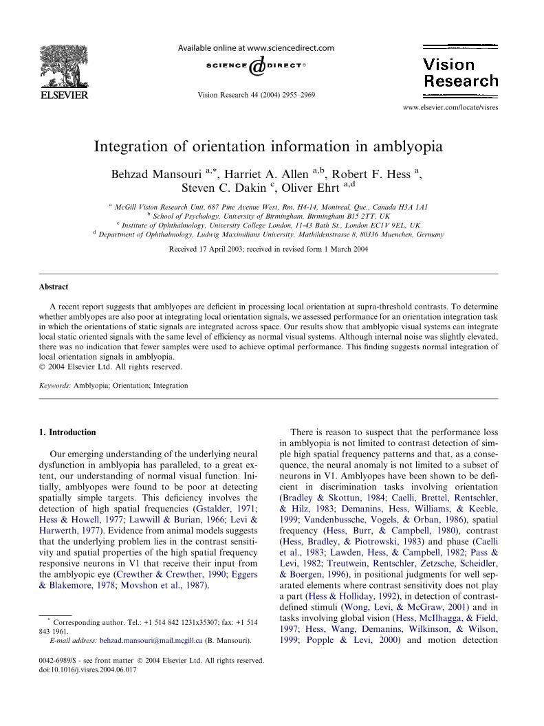
Fig. 1. Stimuli. Arrays of 16 randomly placed, oriented Gabor elements with mean orientation (indicated by the arrow for illustrative purposes only,

not present during testing) relative to the vertical (indicated by the dashed lines for illustrative purposes only, not present during testing). Each Gabor

is a sample from a Gaussian distribution of orientations with a mean equal to the cued orientation and a variable bandwidth. In this figure we show

example stimuli for three different standard deviations of the parent orientation distribution; a standard deviation of 0� (A), 16� (B), and 28� (C).

B. Mansouri et al. / Vision Research 44 (2004) 2955–2969 2957

robs ¼ffiffiffiffiffiffiffiffiffiffiffiffiffiffiffiffiffiffiffiffir2int þ

r2ext

n

r

where robs is the observed threshold, rext is the external

noise, rint is the estimated equivalent intrinsic or internal

noise and n is the estimated number of samples being em-

ployed. In terms of the orientation discrimination task,

robs corresponds to the threshold for orientation discrim-ination, rext to the standard deviation of the distribution

from which the samples are derived (see Section 2), rint tothe noise associated with the measurement of each orien-

tation sample and their combination and n corresponds

to the estimated number of orientation samples being

combined by the visual system.

Assumptions underlying equivalent noise:

(1) Orientation integration involves averaging. Effi-ciency on our tasks indicates that observers invariably

employ more than one sample, i.e. they are combin-

ing information across space and are not relying on a

single element to perform the task. This does not mean

observers necessarily use the average (although this

would be optimal); other strategies, such as using a peak

in the orientation statistics, might also suffice. However,

by employing textures composed of orientation drawnfrom skewed distributions Dakin and Watt (1994) were

able to show that observers� performance was consistent

with their using the average orientation and not the

peak.

(2) Nature of the noise. Equivalent noise assumes

that performance is limited by additive and multiplica-

tive noise. Additive noise is due to noise on the detectors

registering local orientation and could, for example, beplausibly linked to the finite orientation bandwidth of

cells in V1. Sampling efficiency is equivalent to a global

multiplicative noise source; i.e. one that increases with

the strength of signal being pooled. Multiplicative noise

is a ubiquitous feature of neural systems and has been

observed in neurons responsible for integration along

other stimulus dimensions, e.g. motion; MT neurons

(Britten, Shadlen, Newsome, & Movshon, 1993).

(3) Constant internal noise. The two parameters of

internal noise and sampling efficiency in the standard

equivalent noise function are fixed across all levels of

external noise. This assumption is made on the grounds

of parsimony; we do not need to change noise levels as afunction of stimulus variance to account for our data.

In the main experiment, observers viewed an array of

16 randomly positioned, oriented Gabors that were

samples from an orientation distribution whose stand-

ard deviation was varied. The task was to determine

whether the mean orientation of the array was clockwise

or counterclockwise (see Fig. 1) from vertical. The re-

sults were fitted by the equivalent noise model, describedabove, to derive the measures of internal noise and num-

ber of samples. To ensure that any differences between

these measures for normal and amblyopic observers

were due solely to integrative function, we equated per-

formance for a single Gabor element for a similar orien-

tation task. This ensured that performance was equated

for this task for an individual element and that therefore

any difference in the derived measures must be the re-sults of integration per se.

2. Methods

2.1. Observers

Ten normal and twelve amblyopic observers were re-cruited for this experiment. Two of the normal observers

were the authors. The others were naı̈ve to the purpose

of experiment. All observers were optically corrected if

necessary. Clinical details of amblyopic observers are

presented in Table 1. Eye dominance in normal observ-

ers was assessed for each subject using a sighting test

(Rosenbach, 1903).

2.2. Stimuli

The stimuli were arrays of Gabor micro-patterns pre-

sented on a mid-gray background. The envelope of the

Table 1

Clinical details of the amblyopic observers participating in the experiment

Observers Age Type Refraction Acuity Strabismus History, stereo

AM 31 yr RE �3.75 DS 20/50 ET + 3� Detected age 3 yr, patching for 3 yr

Strab �3.25 DS 20/25

LN 49 yr RE +3.75�3.75 120� 20/30 ET + 10� Detected age 3 yr, glasses since, patching 6w,

strabismus surgery RE age 20 yrStrab +3.00�2.00 80� 20/20

MA 22 yr LE �0.25 DS 20/15 Ortho Detected age 3 yr, patching for 4 yr, glasses for 8 yr

Aniso +3.50�0.50 0� 20/200

MG 28 yr RE �0.50 DS 20/100 ET + 1� Detected age 4 yr, patching for 6 months, no surgery

Strab +0.50 DS 20/15

MM 27 yr LE +0.25�1.75 135� 20/20 Ortho Detected age 6 yr, 6 months patching basic stereovision present

Aniso +0.75�3.50 55� 20/30

NG 30 yr RE +5.00�2.00 120� 20/70 ET + 8� Detected age 5 yr, patching for 3 months, no glasses tolerated,

2 strabismus surgery RE age 10–12 yrMixed +3.50�1.00 75� 20/20

RB 49 yr LE +3.25 DS 20/15 Detected age 6 yr, glasses since 6 yr, no other therapy,

near normal local stereo visionAniso +4.75�0.75 45� 20/40 XT � 5�

VL 35 yr LE +0.50 DS 20/20 Detected age 6 yr, /Aniso +3.50�3.00 50� 20/50 Ortho

YC 31 yr LE +2.00 DS 20/15 ET + 10� Detected age 2 yr, patching for 4 yr, glasses for 16 yr

Strab +2.00 DS 20/40

BB 58 yr LE +0.50�0.50 20/15 Detected age 8 yr, surgery to correct angle of large eso,

patching for 6 monthsStrab +1.25�0.25 20/600 ET + 5�

AT 21 yr LE +0.50 DS 20/15 Ortho Detected age 3 yr, glasses since 8 yr no other therapy

Aniso +0.50�2.0 200� 20/30

PH 33 yr LE �2.0+0.50 DS 20/25 ET + 5� Detected age 4 yr, patching for 6 months, surgery when he was 5 yr

Strab +0.50 DS 20/63

The following abbreviations have been used; strab for strabismus, aniso for anisometropic, RE for right eye, LE for left eye, ET for esotropia, XT for

exotropia, ortho for orthotropic alignment, sph for dioptre sphere.


Gabor had a standard deviation of 0.4�. The spatial fre-quency of sinusoidal modulation within the Gabor was

varied between 0.52 cycles per degree (cpd) and 4.16

(cpd) depending on the experiment. Gray levels of

patches were added when they overlapped and clipped

appropriately at the maximum or minimum gray level

when they were outside the range of the screen, although

this only happened rarely. The Gabors were randomlydistributed in a circular area, which varied between 3�and 12� wide. The center of the distribution was the cen-

ter of the screen. The orientation in each Gabor micro-

pattern was selected from a Gaussian distribution with a

mean equal to the cued orientation, i.e. 90�± the cue

generated by APE, an adaptive method of constant

stimuli (Watt & Andrews, 1981) and a variable band-

width. The distribution�s standard deviation, r, was var-ied from 0� (all elements aligned) to 28� (high

orientation variability) as shown in Fig. 1. The dotted

lines and arrows in Fig. 1 represents the notional vertical

and mean orientation of the array.

2.3. Apparatus

An Apple Macintosh G3 computer was utilized in the

experiment. The Matlab environment (MathWorks

Ltd.) and Psychophysics ToolBox (Brainard, 1997) were

used for programming. All stimuli were displayed on a

20 in. Sony monitor (Trinitron 520GS), which was cali-

brated and linearized using Graseby S370 photometerand the Video Toolbox (Pelli, 1997) package. Pseudo

12 bit contrast accuracy was achieved by using a video

attenuator (Pelli & Zhang, 1991), which combined the

RBG outputs of the graphic card (ATI Rage 128) into

the G gun. The monitor had a refresh rate of 75 Hz.

The mean luminance of the screen was 33 cd/m2 and

the resolution was 1152 · 870 pixels. One pixel on the

screen was 0.32 mm, which was 2.12 0 of the observers�visual angle from the viewing distance of 52 cm. The

observers performed the task monocularly beginning

with the fellow fixing eye (in amblyopes) and dominant

eye (in normals), with the other eye patched.

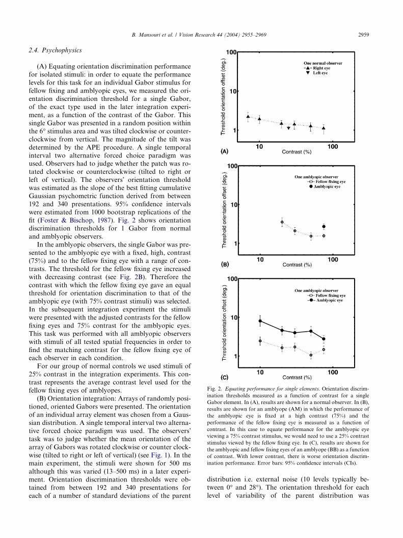
Fig. 2. Equating performance for single elements. Orientation discrim-

ination thresholds measured as a function of contrast for a single

Gabor element. In (A), results are shown for a normal observer. In (B),

results are shown for an amblyope (AM) in which the performance of

the amblyopic eye is fixed at a high contrast (75%) and the

performance of the fellow fixing eye is measured as a function of

contrast. In this case to equate performance for the amblyopic eye

viewing a 75% contrast stimulus, we would need to use a 25% contrast

stimulus viewed by the fellow fixing eye. In (C), results are shown for

the amblyopic and fellow fixing eyes of an amblyope (BB) as a function

of contrast. With lower contrast, there is worse orientation discrim-

ination performance. Error bars: 95% confidence intervals (CIs).


2.4. Psychophysics

(A) Equating orientation discrimination performance

for isolated stimuli: in order to equate the performance

levels for this task for an individual Gabor stimulus for

fellow fixing and amblyopic eyes, we measured the ori-entation discrimination threshold for a single Gabor,

of the exact type used in the later integration experi-

ment, as a function of the contrast of the Gabor. This

single Gabor was presented in a random position within

the 6� stimulus area and was tilted clockwise or counter-

clockwise from vertical. The magnitude of the tilt was

determined by the APE procedure. A single temporal

interval two alternative forced choice paradigm wasused. Observers had to judge whether the patch was ro-

tated clockwise or counterclockwise (tilted to right or

left of vertical). The observers� orientation threshold

was estimated as the slope of the best fitting cumulative

Gaussian psychometric function derived from between

192 and 340 presentations. 95% confidence intervals

were estimated from 1000 bootstrap replications of the

fit (Foster & Bischop, 1987). Fig. 2 shows orientationdiscrimination thresholds for 1 Gabor from normal

and amblyopic observers.

In the amblyopic observers, the single Gabor was pre-

sented to the amblyopic eye with a fixed, high, contrast

(75%) and to the fellow fixing eye with a range of con-

trasts. The threshold for the fellow fixing eye increased

with decreasing contrast (see Fig. 2B). Therefore the

contrast with which the fellow fixing eye gave an equalthreshold for orientation discrimination to that of the

amblyopic eye (with 75% contrast stimuli) was selected.

In the subsequent integration experiment the stimuli

were presented with the adjusted contrasts for the fellow

fixing eyes and 75% contrast for the amblyopic eyes.

This task was performed with all amblyopic observers

with stimuli of all tested spatial frequencies in order to

find the matching contrast for the fellow fixing eye ofeach observer in each condition.

For our group of normal controls we used stimuli of

25% contrast in the integration experiments. This con-

trast represents the average contrast level used for the

fellow fixing eyes of amblyopes.

(B) Orientation integration: Arrays of randomly posi-

tioned, oriented Gabors were presented. The orientation

of an individual array element was chosen from a Gaus-sian distribution. A single temporal interval two alterna-

tive forced choice paradigm was used. The observers�task was to judge whether the mean orientation of the

array of Gabors was rotated clockwise or counter clock-

wise (tilted to right or left of vertical) (see Fig. 1). In the

main experiment, the stimuli were shown for 500 ms

although this was varied (13–500 ms) in a later experi-

ment. Orientation discrimination thresholds were ob-tained from between 192 and 340 presentations for

each of a number of standard deviations of the parent

distribution i.e. external noise (10 levels typically be-

tween 0� and 28�). The orientation threshold for each

level of variability of the parent distribution was


estimated as the slope of the best fitting cumulative

Gaussian function using a maximum likelihood proce-

dure. The model described in the introduction was fitted

to the thresholds separately for each eye of each obser-

ver in each condition.

2.5. Statistics

We tested the parameters from our equivalent noise

model, internal noise and number of samples separately.

In order to compare the differences between the groups,

we used a 2 (between) · 2 (within) · 3 (within) analysis

of variance (ANOVA) for the variables of observer (nor-

mal and amblyopic), eye (amblyopic and fellow fixing inamblyopic observers and dominant and non-dominant

in normal observers) and spatial frequency (low, med-

ium and high). We also calculated 95% confidence inter-

vals for the thresholds from each individual

psychometric function and used it to compare individual

sets of data within the groups.

3. Experimental manipulations

3.1. Integration within different spatial frequency bands

In the first experiment low spatial frequency stimuli

(0.52 cpd), which were well within the acuity limit of

all observers, were tested in 10 amblyopic and 10 normal

observers. In each trial, 16 micro-patterns were pre-sented within the stimulus area (see Fig. 1). The stimulus

area was 6� of visual angle. The exposure duration time

was 500 ms.

Since contrast sensitivity is similar to normal in the

majority of amblyopes for low spatial frequencies (Hess

& Howell, 1977), these stimuli are useful to compare the

integration function of the amblyopic and normal eyes

with a stimulus for which contrast thresholds are normalor only minimally affected.

In order to better understand the influences of differ-

ent spatial frequencies on orientation integration for the

amblyopic visual system, 6 amblyopic (AM, LN, MA,

MG, MM and RB, see Table 1) and 6 normal observers

were tested with medium and high spatial frequency Ga-

bor arrays. The spatial frequency of the high frequency

stimulus was a factor of 2 below the highest spatial fre-quency that the observers reported that they could see––

except in the (MA) case where this led to a very high ori-

entation discrimination threshold (87�), so the spatial

frequency was reduced by a further factor of 2. The

average high spatial frequency stimuli were about a fac-

tor of 6–8 (3.12–4.16 cpd) above the low frequency stim-

uli (0.52 cpd). These were stimuli for which contrast

thresholds were elevated in amblyopic eyes. The mediumfrequency stimuli typically were between the high and

low spatial frequencies (e.g. 2 cpd).

3.2. Exposure duration

While some studies have argued that amblyopic vis-

ual system is more detrimentally affected by decreasing

the exposure duration than the normal visual system

(Rentschler & Hilz, 1985; Weiss, Rentschler, & Caelli,1985), others have shown very little effect of decreasing

exposure duration (Demanins & Hess, 1996a; Loshin

& Jones, 1982). The discrepancy may be due to the dif-

ferent tasks studied, in the former case it was vernier

acuity and phase discrimination, whereas in the latter

it was contrast thresholds and positional sensitivity for

well separated stimuli. To ascertain whether exposure

duration is important for local orientation integrationin amblyopia, we measured integration performance

for a range of exposure durations, between 13 ms and

500 ms. This was done in one normal and five amblyopic

observers (MA, PH, RB, MM and BB).

3.3. Numerosity, density and stimulus extent

It has been previously shown in normal observers(Dakin, 2001) that the number of presented elements re-

lates strongly to the sampling efficiency of an observer

and the internal noise can be affected by the density of

the element array. To better understand the mechanisms

involved in integration by the amblyopic visual system,

we varied these parameters in one normal and five

amblyopic observers (MA, AT, PH, RB and MM).

Three parameters were varied in this experiment;number, density of elements and radius of stimulus area.

Since these parameters are inter-related, changing one

without changing the others is not possible. Therefore

to study the effects of these parameters individually,

one variable was kept fixed at a time, whilst allowing

the other two to co-vary. In the first condition, radius

of stimulus area was held constant (6�) and the number

of elements (16, 64 and 256) and the density (0.176,0.705 and 2.820 element/cm2) co-varied. In the second

condition, the number of elements was held constant

(64) and the radius of stimulus area (3�, 6� and 12�)and the density (2.820, 0.705 and 0.176 element/cm2)

co-varied. In the third condition, the density was held

constant (0.705 element/cm2) and the radius of stimulus

area (3�, 6� and 12�) and the number of elements (16, 64

and 256) co-varied. In all conditions, the presentationtime was 500 ms.

4. Results

4.1. Equating orientation performance levels

Fig. 2A shows the relationship between the orienta-tion discrimination threshold for a single Gabor and

contrast for a normal observer. Performance is relatively

Fig. 3. (A) One element orientation threshold in amblyopic observers.

Comparison of mean one element discrimination threshold of ambly-

opic eyes (contrast 75%) (filled bars), fellow fixing eyes (contrast 75%)

(dotted bars) and fellow fixing eyes (contrast 20%) (gray bars) for

tested spatial frequencies are presented. Error bars represent ±0.5 SD.

There are significant differences in discrimination thresholds between

the amblyopic and fellow fixing eyes ( p<0.05), which are more

prominent with stimuli with high spatial frequency ( p<0.01). Decreas-

ing the contrast of the stimuli to 20% for the fellow fixing eyes

increased the mean threshold, especially in high spatial frequency

condition. (B) Multi element orientation thresholds. The average

threshold from the amblyopic eyes (filled bars) and fellow fixing eyes

(gray bars) and average of the dominant and non-dominant eyes of

normal observers (open bars) are compared for all tested spatial

frequencies when all the 16 stimuli are aligned (SD = 0). Error bars

represent ±0.5 SD. In all spatial frequency conditions the thresholds of

the amblyopic, fellow fixing and normal eyes are not significantly

different ( p>0.05). Also, there is no significant difference between the

various spatial frequencies ( p>0.05).


constant at high contrasts but deteriorates as the con-

trast is reduced (Hess, Ledgeway, & Dakin, 2000). Sim-

ilar threshold performance at one contrast level is seen

for the non-dominant eye (inverted triangle) of this nor-

mal observer. In Fig. 2B an example is shown of data

equating the performance levels between fellow fixingand amblyopic eyes of our amblyopic observers. The

filled symbol represents the orientation discrimination

performance of the amblyopic eye for a fixed 75% con-

trast stimulus. The open symbols and dotted curve rep-

resent the performance of the fellow fixing eye as a

function of stimulus contrast. In this case, to equate per-

formance levels for the single element, the contrast of

the stimuli for the fellow fixing eye needs to be reducedto a third (i.e. 25%) of that seen by the amblyopic eye.

We repeated these measurements for all amblyopic

observers and used the appropriate contrast for the fel-

low fixing eye that equated orientation discrimination

performance for 75% contrast stimuli seen by the ambly-

opic eye. In Fig. 2C, we show how the amblyopic eyes�performance (filled symbols and solid curve) changes

with reducing the contrast below 75%. It exhibits astronger dependence on contrast than that seen for the

fellow fixing eye (unfilled symbols and dotted curve)

which was expected due to the known poor performance

for orientation discrimination for amblyopic observers

when using low contrast stimuli (Demanins et al., 1999).

Averaged results for the orientation discrimination of

an isolated Gabor are shown in Fig. 3A for fellow fixing

eyes at two contrast levels and amblyopic eyes for thethree spatial frequencies tested. At the same physical

contrast, the amblyopic eye exhibits poorer orientation

discrimination compared with the fellow fixing eye

( p<0.05) although the magnitude of this effect is only

large at high spatial frequencies. When the contrast of

the fellow fixing eye is reduced to around 20% there

was no statistically significant difference between the

performance of the fellow fixing and amblyopic eyes.

4.2. Integrating local oriented signals

The results shown in Fig. 3B represent a similar com-

parison to that in 3A for an array of identically oriented

Gabors. Here we compared mean orientation perform-

ance for the amblyopic (75% contrast) and fellow fixing

eyes (adjusted contrast) and the normal eyes of non-amblyopic observers (25% contrast). There is no statisti-

cally significant difference between the means of these

three conditions indicating that our method of equating

performance between the amblyopic eyes, fellow fixing,

and normal eyes was successful. Notice that the orienta-

tion thresholds for the high spatial frequency Gabors

are much reduced in the multiple element, compared

with the isolated element, condition. It would seem thatthe reduced orientation discrimination performance for

isolated high spatial frequency Gabors (Fig. 3A) may

be due to either an inability to detect some stimuli when

their position is uncertain or to the benefit of being able

to integrate a number of identical individual signals.

Our next step was to compare performance for the

mean orientation task when the individual Gaborelements within the array did not have identical orienta-

tions. As illustrated in Fig. 1 we introduced orienta-

tional variability into the display by having the

orientation of each Gabor element be a sample from a

parent Gaussian orientation distribution whose mean

was at the vertical ± the cued orientation. We measured

the threshold orientation offset required to reach crite-

rion performance on this mean orientation task as afunction of the standard deviation of the distribution

from which the individual orientation samples were


drawn. Example results of a normal observer (A) and an

amblyopic observer (B) are displayed in Fig. 4. The dis-

crimination threshold for judging the mean orientation

of an array of 16 randomly positioned Gabors is plotted

against the standard deviation of the orientation distri-

bution. The error bars represent 95% confidence inter-vals obtained from our bootstrapping procedure. The

curves represent the equivalent noise model described

in the introduction fitted to the orientation thresholds

with the best fit estimates for internal noise (IN) and

number of samples (NS) values shown in the inset. In

the case of the normal observer (Fig. 4A), performance

of the right (dominant––open symbols and dotted curve)

and left (non-dominant––filled symbols and solid curve)eyes are consistent with approximately 6.2 and 5.0 out of

the 16 available samples being used to estimate the mean

Fig. 4. Mean orientation thresholds. Orientation discrimination thresh-

olds are plotted against the standard deviation of the orientation

distribution from which the samples were taken. In this case, 16

Gabors comprised the stimulus array. The curve is the best fit for the

equivalent noise model. The error bars represent 95% confidence

intervals. The parameters of this fit, internal noise (IN) and number of

samples (NS) are shown in the inset. In (A), results are shown for

dominant (open symbols and dotted curve) and non-dominant (filled

symbols and solid curve) eyes of a normal observer (HA) whereas in

(B), results are shown for the amblyopic (filled symbols and solid

curve) and fellow fixing (open symbols and dotted curve) eyes of a

strabismic amblyope (MA).

orientation of the Gabor array, respectively. The esti-

mate of internal noise was 1.1� and 1.6�. The results in

Fig. 4B compare performance for the fellow fixing (open

symbols and dotted curve) and amblyopic eyes (filled

symbols and solid curve) of one of our amblyopic

observers (RA). This is a typical result showing similarperformance with the fellow fixing and amblyopic eyes

of this individual. The internal noise and number of

samples in the amblyopic eye (2.0� and 6.3�) were not

significantly different from those of the fellow fixing

eye (2.3� compared with 5.2�).

4.3. Integration for different spatial frequencies

In Fig. 5 we show results in a similar form to that

described above but averaged over the eyes of our nor-

mal and amblyopic observers. In each case, we plot

Low spatial frequency (mean threshold)

05

10152025303540

0 1 2 4 6 8 12 16 20 28Standard Deviation (degrees)

Thre

shol

d (d

egre

es)

05

10152025303540


Thre

shol

d (d

egre

es)

05

10152025303540


Thre

shol

d (d

egre

es)

Dominant Eye

Non-dominantEyeFellow FixingEyeAmblyopic Eye

Medium spatial frequency (mean threshold)

High spatial frequency (mean threshold)

(C)

(B)

(A)

Fig. 5. Average mean orientation thresholds. Averaged thresholds are

displayed for the amblyopic (filled circles and solid lines) eyes, the

fellow fixing eyes (open circles and dotted curve) and eyes of normal

observers (open and filled square symbols correspond to dominant and

non dominant eyes, respectively) for stimuli of low (A), medium (B)

and high (C) spatial frequency. The error bars represent ±0.5 SD.


the averaged thresholds for each eye of our normal

observers (dominant and non-dominant eyes) and for

each eye of our amblyopes (fellow fixing and ambly-

opic). The error bars represent ±0.5 standard deviation

(SD) of the population. We did not find any significant

differences between the thresholds from normal andamblyopic eyes. This was true for all low (Fig. 5A), med-

ium (Fig. 5B) and high (Fig. 5C) spatial frequencies.

From each individual result we derived the best fits

for the parameters of internal noise and number of sam-

ples and averaged these individually derived measures

across our observer populations. These measures are

shown for the three populations, normals (average

threshold of both eyes of normal observers), fellow fix-ing eyes and amblyopic eyes (of amblyopic observers)

in Fig. 6. For the purpose of clarity, the error bars rep-

resent ±0.5 SD. The internal noise parameter was signif-

icantly higher at high spatial frequencies (fellow fixing

versus amblyopic eye only, p<0.05), however at low

and medium spatial frequencies, internal noise was not

significantly different for amblyopic eyes ( p>0.05). In

terms of the number of samples parameter (Fig. 6B),

Internal noise

00.5

11.5

22.5

33.5

4

Low Medium High Spatial frequency

Low Medium High Spatial frequency

Mea

n in

tern

al n

oise

(d

egre

es)

Fellow fixing eye

Amblyopic eye

Normal eye

Fellow fixing eye

Amblyopic eye

Normal eye

p<0.05

Sampling efficiency

01234567

Num

ber o

f sam

ples

p<0.01

p<0.05

(A)

(B)

Fig. 6. Internal noise and number of samples. Comparison of the

average of the individual estimates of internal noise (A) and number of

samples (B) from our model fits for the three variables of, fellow fixing

eyes (gray bars), amblyopic eyes (filled bars), and eyes of normal

observers (open bars). The error bars represent ±0.5 SD. In (A), there

is significantly higher internal noise for amblyopic eyes compared with

either normal eyes or fellow fixing eyes only at high spatial frequency

condition ( p<0.05). For the number of samples measured in (B), we

found no significant different between amblyopic and either normal

eyes or fellow fixing eyes, although the number of samples, unlike the

internal noise, did show a significant overall reduction with increasing

spatial frequency ( p<0.05).

as the spatial frequency increased, the number of sam-

ples taken by the visual systems decreased, regardless

of being amblyopic or non-amblyopic ( p<0.05 for med-

ium versus high spatial frequency and p<0.01 for low

versus high spatial frequency). There was no significant

difference between the number of samples taken by theamblyopic and non-amblyopic eyes ( p>0.05).

For the purpose of clarity, the internal noise and

number of samples values in each individual amblyopic

(Table 2(panels A and B), respectively) and normal ob-

server (Table 2(panels C and D), respectively) are

presented.

4.4. Exposure duration

The previous results were obtained at an exposure

duration of 500 ms. In Fig. 7A we show the effect of

two presentation durations, 500 ms versus 100 ms on

orientation discrimination performance on our single

element task for one of our amblyopic observers (BB).

Short stimulus durations disadvantage the performance

of the amblyopic eye relative to its fellow fixing eye andtherefore a lower contrast is required for the fellow fix-

ing eye to equate the orientation performance of the fel-

low fixing and amblyopic eyes. However, once

performance for the single element has been equated,

the subsequent integration of oriented signals is not sig-

nificantly different ( p>0.05) for fellow fixing and ambly-

opic eyes (Fig. 7B). Internal noise and number of

samples for five amblyopic observers are presented inTable 3.

For completeness we found that integration of orien-

tation information was quite similar across a wide range

(500–13 ms) of exposure durations in normal vision

(Fig. 7C).

4.5. Numerosity, density and stimulus extent

In our main experiment we used arrays of 16 Gabors,

randomly distributed within an area with radius of 6�,giving a density of 0.705 element/cm2. We wondered to

what extent this initial choice of parameters affected

our conclusions. To test this, we varied the numerosity,

density and stimulus extent of the oriented Gabors for

our integration task with stimuli of the low spatial fre-

quency and compared results for the eyes of one normal(BM) and five amblyopic observers (MA, AT, RA, PH

and MM), which are displayed in Fig. 8 (the error bars

represent 95% confidence intervals). The results from all

of these conditions showed similar patterns of increasing

or decreasing internal noise and number of samples for

all dominant fellow fixing eyes (open symbols and

dashed lines) and non-dominant and amblyopic eyes

(filled symbols and solid lines). Furthermore, in almostall of the variable levels, there were no significant differ-

ences between the values of internal noise and number

Table 2

Internal noise and number of samples in the amblyopic and normal observers

Observers LSF FFE LSF AME MSF FFE MSF AME HSF FFE HSF AME

Panel A

AM 1.43 1.54 0.27 0.87 0.56 0.98

LN 2.35 1.51 0.96 1.14 1.36 2.24

MA 2.39 1.58 1.38 2.37 3.61 3.78

MG 4.43 5.24 3.75 4.83 4.18 6.78

MM 1.51 1.50 1.16 1.34 1.41 2.07

NG 2.76 2.41 N/A N/A N/A N/A

RB 2.49 2.96 2.35 2.67 1.92 1.93

VL 2.51 2.29 N/A N/A N/A N/A

YC 1.78 1.33 N/A N/A N/A N/A

BB 4.08 5.87 N/A N/A N/A N/A

AT 3.79 5.58 N/A N/A N/A N/A

PH 1.82 2.36 N/A N/A N/A N/A

Panel B

AM 5.44 6.58 6.55 2.84 1.16 2.14

LN 3.89 3.07 2.00 2.81 1.20 2.06

MA 5.21 6.24 1.87 3.03 2.01 0.79

MG 2.46 3.49 1.89 1.74 1.87 2.17

MM 2.89 3.47 1.60 2.47 1.12 1.43

NG 2.54 4.52 N/A N/A N/A N/A

RB 1.79 2.26 1.25 1.36 1.36 1.24

VL 4.10 8.69 N/A N/A N/A N/A

YC 8.15 5.08 N/A N/A N/A N/A

BB 1.50 0.75 N/A N/A N/A N/A

AT 3.41 4.26 N/A N/A N/A N/A

PH 5.43 5.61 N/A N/A N/A N/A

Panel C

BM 1.1 1.57 0.72 0.96 1.34 2.09

HA 2.32 2.68 2.07 1.74 3.69 2.00

LA 1.63 1.77 1.25 0.99 1.17 1.80

EK 1.65 1.57 1.03 0.98 1.76 1.82

SD 2.32 2.24 2.39 2.12 3.38 6.77

MA 1.43 1.51 1.31 1.21 2.78 2.66

OE 2.27 1.83 N/A N/A N/A N/A

MM 2.04 1.87 N/A N/A N/A N/A

CH 3.12 3.54 N/A N/A N/A N/A

PA 1.42 1.83 N/A N/A N/A N/A

Panel D

BM 6.24 4.96 3.82 5.24 1.92 1.65

HA 4.77 5.24 2.42 2.92 0.77 1.24

LA 2.95 1.60 1.42 1.58 1.28 1.83

EK 5.25 5.60 3.10 2.88 2.75 2.75

SD 1.80 1.97 1.68 1.71 1.01 0.49

MA 4.91 4.95 4.95 5.05 2.17 0.55

OE 5.18 4.27 N/A N/A N/A N/A

MM 6.67 10.37 N/A N/A N/A N/A

CH 3.18 4.73 N/A N/A N/A N/A

PA 10.74 7.49 N/A N/A N/A N/A

Panel A: internal noise in amblyopic observers; panel B: number of samples in amblyopic observers; panel C: internal noise in normal observers;

panel D: number of samples in amblyopic observers. The following abbreviations have been used; LSF: low spatial frequency, MSF: medium spatial

frequency, HSF: high spatial frequency, FFE: fellow fixing eye, AME: amblyopic eye.


of samples found for amblyopic and fellow fixing eyes.

In the constant radius condition, our data showed that

increasing the number of elements and the density of

the texture has little effect on the magnitude of the inter-

nal noise (Fig. 8A), but it did increase the number of

samples (Fig. 8D). In the constant numerosity condi-

tion, as the radius increased and the density decreased,

the internal noise decreased (Fig. 8B) but the number

of samples did not show a consistent pattern (Fig. 8E).

In the constant density condition, as the number of

Fig. 7. Mean orientation thresholds for different exposure durations. In

(A), orientation discrimination thresholds are plotted for a single

Gabor element for the amblyopic and fellow fixing eyes of a strabismic

amblyope (BB) for two exposure durations (100 and 500 ms). The

amblyopic eye is disadvantaged when the exposure duration is short

and this necessitates a different correction factor to bring the

performance of amblyopic and fellow fixing eyes together for the

single element case. In (B), mean orientation thresholds are plotted

against orientation discrimination standard deviation for an amblyopic

observer (MA). Orientation integration is not significantly different for

two exposure durations (500 and 13 ms). In (C), orientation integra-

tion is seen to be invariant with exposure duration for the dominant

eye of a normal observer (BM). The parameters of this fit, internal

noise (IN) and number of samples (NS) are shown in the inset. The

error bars represent 95% confidence intervals.

Table 3

Internal noise and number of samples in one normal and four

amblyopic observers in 13 ms presentation time condition

Observers Internal noise Number of samples

FFE AME FFE AMB

MA 5.00 2.5 2.28 4.85

PH 2.60 2.91 6.92 9.24

RB 3.56 3.26 1.75 2.55

MM 2.79 4.60 2.00 2.40

BB 5.01 5.95 1.30 0.95

BM (normal) DE 1.47 NDE 1.75 DE 5.42 NDE 4.54

The following abbreviations have been used; FFE: fellow fixing eye,

AME: amblyopic eye, DE: dominant eye, NDE: non-dominant eye.


elements and the radius increased, the internal noise de-

creased (Fig. 8C) and the number of samples increased

(Fig. 8F).

These results highlight the importance of numerosityfor this task. Unlike density or stimulus extent, the num-

erosity appears to determine how many samples are ta-

ken, a result consistent with the previous work of Dakin

(2001) and Allen, Hess, Mansouri, and Dakin (2003).

We find this also to be the case for amblyopic and fellow

fixing eyes. An interesting difference between results for

amblyopic and fellow fixing eyes of the amblyopic

observers in our experiment and normal eyes of normalobservers in the previous work (Dakin, 2001) concerns

the internal noise. Dakin showed that in normals, inter-

nal noise varied with density. We found in our ambly-

opic observers that it varied inversely with the

stimulus extent, although the results are not definite.

5. Discussion

The main finding of our study is that amblyopic

observers can integrate local orientation information

that occurs within different regions of their visual field

just as efficiently as normals. This finding is robust

across a number of stimulus parameters including expo-

sure duration, numerosity, density and stimulus extent.

At the level at which this integration takes place, we findno evidence of either a grossly elevated internal noise or

a reduced number of samples. The amblyopic cortex

processes these stimuli with the same efficiency as that

of the normal cortex or indeed the cortex driven by

the fellow fixing eye.

Previous research has highlighted a number of

processing deficits in amblyopia, these include, contrast

sensitivity, positional uncertainty (Hess & Holliday,1992; Levi & Klein, 1985), global motion (Simmers

et al., 2003), global form (Simmers et al., forthcoming)

and orientation (Barrett et al., 2003; Popple & Levi,

2000). How do the present results relate to these deficits?

Our method of equating performance in terms of the dis-

crimination of a single Gabor element by manipulating

(A) Constant radius (6°)

0

1

2

3

4

5

6

10 100 1000Number of elements

Inte

rnal

noi

se (d

egre

es)

Inte

rnal

noi

se (d

egre

es)

Fellow fixing eye (MA)

Amblyopic eye (MA)

Fellow fixing eye (AT)

Amblyopic eye (AT)

Fellow fixing eye (RA)

Amblyopic eye (RA)

Fellow fixing eye (PH)

Amblyopic eye (PH)

0

5

10

15

20

25

30


Num

ber o

f sam

ples

(B) Constant numerosity (64)

0

1

2

3

4

5

6

1 10 100Radius (degrees)

0

5

10

15

20

25

30

1 10 100Radius (degrees)

Num

ber o

f sam

ples

Num

ber o

f sam

ples

(C) Constant density (37e/10 deg ^2)

(D) Constant radius (6°) (E) Constant numerosity (64) (F) Constant density (37e/10 deg ^2)

0

1

2

3

4

5

6


Inte

rnal

noi

se (d

egre

es)

0

5

10

15

20

25

30


Fig. 8. Effects of various number of elements, presentation area and density on the internal noise and sampling efficiency. In (A) and (D), internal noise

and number of samples estimates are compared for the amblyopic and fellow fixing eyes for the fixed radius condition (density and numerosity co-

vary). In (B) and (E), internal noise and number of samples estimates are compared for the amblyopic and fellow fixing eyes for the fixed numerosity

condition (density and numerosity co-vary). In (C) and (F), internal noise and number of samples estimates are compared for the amblyopic and

fellow fixing eyes for the fixed density condition (radius and numerosity co-vary). The error bars represent 95% confidence intervals.


the contrast of the stimuli presented to the fellow fixingeye had the effect of factoring out any downstream influ-

ence due to differences in contrast sensitivity or local ori-

entation processing between the parts of the visual

system driven by fellow fixing and amblyopic eyes. Fur-

thermore, the fact that the local position of the Gabor

elements within the array was irrelevant to the task

meant that any positional uncertainty that might be pre-

sent at the level of the integration process studied herewould not influence performance. Thus, the present re-

sults are not inconsistent with what we already know

about the amblyopic deficit. They are relevant to the

findings with a similar task requiring integration of mo-

tion where deficits were revealed for amblyopic observers

(Simmers et al., 2003). Our finding that local static sig-

nals can be integrated with normal efficiency in ambly-

opia argues that the deficit in amblyopia does notinvolve integration in general but certain types of inte-

gration in particular. It is unlikely however that a com-

mon mechanism would determine both the integration

of static oriented signals and the direction of moving sig-

nals. From the little we know of the physiology, the for-

mer would take place within the ventral stream and the

latter within the dorsal stream (Mishkin & Ungerleider,

1982). Thus in terms of global integration of visual infor-mation, the dorsal stream may be more disadvantaged in

amblyopia when it comes to processes involving global

integration. Although it should be kept in mind that such

deficits might be highly task specific.

5.1. Special forms of orientation integration

The present findings may be relevant to why amblyo-

pes have similar performance to normals when detecting

textures based on orientational contrast (Mussap &

Levi, 1999). Such texture discriminations however, in

principle, can be accomplished by local processes involv-

ing orientation discrimination at the edge of the texture-

defined region. The present findings are consistent withthe conclusions of two earlier studies concerning special

forms of orientation integration, in which the encoding

of spatial position is a key factor, namely contour inte-

gration (Hess et al., 1997) and global shape discrimina-

tion (Hess et al., 1999). Amblyopes may be anomalous

at these special forms of orientation integration not be-

cause their integration of orientation signals per se is

necessarily anomalous but because of poor positionalencoding (Demanins & Hess, 1996b; Hess & Holliday,

1992; Levi & Klein, 1985).

5.2. Explanations for amblyopia

There are three competing explanations for the neural

nature of the underlying anomaly in amblyopia; loss of

cells (Levi & Klein, 1986), disarray of cells (Hess, Camp-bell, & Greenhalgh, 1978) or anomalous interaction be-

tween cells (Hess, Campbell, & Zimmern, 1980; Polat,

Sagi, & Norcia, 1997). Although there is no reason to

expect that these explanations are mutually exclusive,


let us for simplicity consider that they are. The above

explanations are sufficiently vague that it is difficult to

know to what extent the present results support or refute

them. Some general comments can be made but it

should be kept in mind that they relate specifically to

the type of model used here to fit the data.

5.3. Loss of cells

Our measure of the number of samples comes from

the statistical nature of the task. It does not, therefore,

relate simply to the number of neural samples taken

by the amblyopic visual system. It is really a general

measure of efficiency. If there were fewer samples takenby the amblyopic visual system at any point up to the

site where orientation integration takes place, one would

expect to see a reduction in our ‘‘number of samples’’

measure.

5.4. Disarray of cells

Since the individual Gabors within our arrays wererandomly positioned, any purely positional disarray

involving cells with orientation tuning would not be ex-

pected to affect the type of integration we report here. If

the positional disarray were at the input stage (i.e.

involving the lay-out of the non-oriented sub-units) to

cells with orientation tuning, one might expect an anom-

aly to local orientation processing which in our case is

corrected for in our initial equating experiment. If thedisarray occurs within the orientation domain, one

would expect to see an elevated level of internal noise,

which we did observe, but it was of small magnitude

and restricted to high spatial frequencies.

5.5. Anomalous interactions between cells

We found that the efficiency of integration in ambly-opia did not depend on the spatial arrangement of the

local oriented signals (numerosity, density or spatial ex-

tent). A particularly revealing case is where multiple ele-

ments are used but integration is not required (i.e. where

the distribution SD = 0; see Fig. 3B). In this case, at high

spatial frequencies where we show the integration of

orientation is defective in amblyopic eyes, performance

in the case where the standard deviation was zero, isnot significantly different between normal and ambly-

opic eyes. This suggests that there were no detrimental

effects in the multi-element case per se due to lateral

interactions. We can therefore rule out anomalous lat-

eral interactions of the most general form occurring be-

fore the site of integration for the type of integration

measured here. However, our results do not bear on

some more specific types of anomalies between neigh-bouring elements that does not affect their later

integration.

Acknowledgment

This work was supported by a Canadian Institute for

Health Research (CIHR) grant (MOP 108-18) to Robert

F. Hess.

References

Ahumada, A. J., Jr., & Watson, A. B. (1985). Equivalent-noise model

for contrast detection and discrimination. Journal of Optical

Society of America A: Optics, Image Sciences, and Vision, 2(7),

1133–1139.

Allen, H. A., Hess, R. F., Mansouri, B., & Dakin, S. C. (2003).

Integration of first- and second-order orientation. Journal of

Optical Society of America A: Optics, Image Sciences, and Vision,

20(6), 974–986.

Baker, C. L. J., Hess, R. F., & Zihl, J. (1991). Residual motion

perception in a ‘‘motion-blind’’ patient, assessed with limited-

lifetime random dot stimuli. Journal of Neuroscience, 11(2),

454–461.

Barlow, H. B. (1957). Increment thresholds at low intensities consid-

ered as signal/noise discriminations. Journal of Physiology, 136(3),

469–488.

Barrett, B. T., Pacey, I. E., Bradley, A., Thibos, L. N., & Morrill, P.

(2003). Nonveridical visual perception in human amblyopia.

Investigative Ophthalmology and Visual Sciences, 44(4), 1555–1567.

Bradley, A., & Skottun, B. C. (1984). The effects of large orientation

and spatial frequency differences on spatial discriminations. Vision

Research, 24(12), 1889–1896.

Brainard, D. H. (1997). The psychophysics toolbox. Spatial Vision,

10(4), 433–436.

Britten, K. H., Shadlen, M. N., Newsome, W. T., & Movshon, J. A.

(1992). The analysis of visual motion: a comparison of neuronal

and psychophysical performance. Journal of Neuroscience, 12(12),

4745–4765.

Britten, K. H., Shadlen, M. N., Newsome, W. T., & Movshon, J. A.

(1993). Responses of neurons in macaque MT to stochastic motion

signals. Visual Neuroscience, 10(6), 1157–1169.

Caelli, T., Brettel, H., Rentschler, I., & Hilz, R. (1983). Discrimination

thresholds in the two-dimensional spatial frequency domain. Vision

Research, 23(2), 129–133.

Crewther, D. P., & Crewther, S. G. (1990). Neural site of strabismic

amblyopia in cats: spatial frequency deficit in primary cortical

neurons. Experimental Brain Research, 79(3), 615–622.

Dakin, S. C. (2001). Information limit on the spatial integration of

local orientation signals. Journal of Optical Society of America A:

Optics, Image Sciences, and Vision, 18(5), 1016–1026.

Dakin, S. C., & Watt, R. J. (1994). Detection of bilateral symmetry

using spatial filters. Spatial Vision, 8(4), 393–413.

Demanins, R., & Hess, R. F. (1996a). Effect of exposure duration on

spatial uncertainty in normal and amblyopic eyes. Vision Research,

36(8), 1189–1193.

Demanins, R., & Hess, R. F. (1996b). Positional loss in strabismic

amblyopia: inter-relationship of alignment threshold, bias, spatial

scale and eccentricity. Vision Research, 36(17), 2771–2794.

Demanins, R., Hess, R. F., Williams, C. B., & Keeble, D. R. (1999).

The orientation discrimination deficit in strabismic amblyopia

depends upon stimulus bandwidth. Vision Research, 39(24),

4018–4031.

Eggers, H. M., & Blakemore, C. (1978). Physiological basis of

anisometropic amblyopia. Science, 201(4352), 264–267.

Foster, D. H., & Bischop, W. F. (1987). Bootstrap variance estimators

for the parameters of small-sample sensory-performance functions.

Biological Cybernetics, 57(4–5), 341–347.


Gstalder, R. J. (1971). Laser inferometric acuity in amblyopia. Journal

of Pediatric Ophthalmology, 8, 251–256.

Heeley, D. W. (1987). Spatial frequency discrimination for sinewave

gratings with random, bandpass frequency modulation: evidence

for averaging in spatial acuity. Spatial Vision, 2(4), 317–335.

Heeley, D. W., Buchanan-Smith, H. M., Cromwell, J. A., & Wright, J.

S. (1997). The oblique effect in orientation acuity. Vision Research,

37(2), 235–242.

Hess, R. F., & Anderson, S. J. (1993). Motion sensitivity and spatial

undersampling in amblyopia. Vision Research, 33(7), 881–896.

Hess, R. F., Bradley, A., & Piotrowski, L. (1983). Contrast-coding in

amblyopia. I. Differences in the neural basis of human amblyopia.

Proceeding of the Royal Society of London, Series B: Biological

Sciences, 217(1208), 309–330.

Hess, R. F., Burr, D. C., & Campbell, F. W. (1980). A preliminary

investigation of neural function and dysfunction in amblyopia––

III. Co-operative activity of amblyopic channels. Vision Research,

20(9), 757–760.

Hess, R. F., Campbell, F. W., & Greenhalgh, T. (1978). On the nature

of the neural abnormality in human amblyopia; neural aberrations

and neural sensitivity loss. Pflugers Archiv––European Journal of

Physiology, 377(3), 201–207.

Hess, R. F., Campbell, F. W., & Zimmern, R. (1980). Differences in the

neural basis of human amblyopias: the effect of mean luminance.

Vision Research, 20(4), 295–305.

Hess, R. F., & Dakin, S. C. (1999). Contour integration in the

peripheral field. Vision Research, 39(5), 947–959.

Hess, R. F., & Holliday, I. E. (1992). The spatial localization deficit in

amblyopia. Vision Research, 32(7), 1319–1339.

Hess, R. F., & Howell, E. R. (1977). The threshold contrast sensitivity

function in strabismic amblyopia: evidence for a two type classi-

fication. Vision Research, 17(9), 1049–1055.

Hess, R. F., Ledgeway, T., & Dakin, S. (2000). Impoverished second-

order input to global linking in human vision. Vision Research,

40(24), 3309–3318.

Hess, R. F., McIlhagga, W., & Field, D. J. (1997). Contour integration

in strabismic amblyopia: the sufficiency of an explanation based on

positional uncertainty. Vision Research, 37(22), 3145–3161.

Hess, R. F., Wang, Y. Z., Demanins, R., Wilkinson, F., & Wilson, H.

R. (1999). A deficit in strabismic amblyopia for global shape

detection. Vision Research, 39(5), 901–914.

Hess, R. H., Baker, C. L., Jr., & Zihl, J. (1989). The ‘‘motion-blind’’

patient: low-level spatial and temporal filters. Journal of Neuro-

science, 9(5), 1628–1640.

Kiorpes, L., Kiper, D. C., O�Keefe, L. P., Cavanaugh, J. R., &

Movshon, J. A. (1998). Neuronal correlates of amblyopia in the

visual cortex of macaque monkeys with experimental strabismus

and anisometropia. Journal of Neuroscience, 18(16), 6411–6424.

Lawden, M. C., Hess, R. F., & Campbell, F. W. (1982). The

discriminability of spatial phase relationships in amblyopia. Vision

Research, 22(8), 1005–1016.

Lawwill, T., & Burian, H. M. (1966). Luminance, contrast function

and visual acuity in functional amblyopia. American Journal of

Ophthalmology, 62(3), 511–520.

Levi, D. M., & Klein, S. A. (1985). Vernier acuity, crowding and

amblyopia. Vision Research, 25(7), 979–991.

Levi, D. M., & Klein, S. A. (1986). Sampling in spatial vision. Nature,

320(6060), 360–362.

Levi, M., & Harwerth, R. S. (1977). Spatio-temporal interactions in

anisometropic and strabismic amblyopia. Investigative Ophthal-

mology and Visual Science, 16(1), 90–95.

Loshin, D. S., & Jones, R. (1982). Contrast sensitivity as a function of

exposure duration in the amblyopic visual system. American

Journal of Optometry and Physiological Optics, 59(7), 561–567.

Mishkin, M., & Ungerleider, L. G. (1982). Contribution of striate

inputs to the visuospatial functions of parieto-preoccipital cortex in

monkeys. Behavioural Brain Research, 6(1), 57–77.

Morrone, M. C., Burr, D. C., & Vaina, L. M. (1995). Two stages of

visual processing for radial and circular motion. Nature, 376(6540),

507–509.

Movshon, J. A., Adelson, E. H., Gizzi, M. S., & Newsome, W. T.

(1985). The analysis of moving visual patterns in Pattern Recognition

mechanisms. Rome: Vatican press, pp. 117–151.

Movshon, J. A., Eggers, H. M., Gizzi, M. S., Hendrickson, A. E.,

Kiorpes, L., & Boothe, R. G. (1987). Effects of early unilateral blur

on the macaque�s visual system. III. Physiological observations.

Journal of Neuroscience, 7(5), 1340–1351.

Mussap, A. J., & Levi, D. M. (1999). Orientation-based texture

segmentation in strabismic amblyopia. Vision Research, 39(3),

411–418.

Newsome, W. T., & Pare, E. B. (1988). A selective impairment of

motion perception following lesions of the middle temporal visual

area (MT). Journal of Neuroscience, 8(6), 2201–2211.

Pardhan, S. (2004). Contrast sensitivity loss with aging: sampling

efficiency and equivalent noise at different spatial frequencies.

Journal of Optical Society of America A: Optics, Image Sciences,

and Vision, 21(2), 169–175.

Pass, A. F., & Levi, D. M. (1982). Spatial processing of complex

stimuli in the amblyopic visual system. Investigative Ophthalmology

and Visual Science, 23(6), 780–786.

Pelli, D. G. (1997). The VideoToolbox software for visual psycho-

physics: transforming numbers into movies. Spatial Vision, 10(4),

437–442.

Pelli, D. G., & Zhang, L. (1991). Accurate control of contrast on

microcomputer displays. Vision Research, 31(7–8), 1337–1350.

Polat, U., Sagi, D., & Norcia, A. M. (1997). Abnormal long-range

spatial interactions in amblyopia. Vision Research, 37, 737–744.

Popple, A. V., & Levi, D. M. (2000). Amblyopes see true alignment

where normal observers see illusory tilt. Proceedings of the National

Academy of Sciences of the United States of America, 97(21),

11667–11672.

Rentschler, I., & Hilz, R. (1985). Amblyopic processing of positional

information. Part 1: Vernier acuity. Experimental Brain Research,

60(2), 270–278.

Rizzo, M., Nawrot, M., & Zihl, J. (1995). Motion and shape

perception in cerebral akinetopsia. Brain, 118(Pt. 5), 1105–1127.

Rosenbach, O. (1903). Ueber monokulare Vorherrschaft beim binik-

ularen Sehen. Munchener Medizinische Wochenschriff, 30,

1290–1292.

Salzman, C. D., Murasugi, C. M., Britten, K. H., & Newsome, W. T.

(1992). Microstimulation in visual area MT: effects on direction

discrimination performance. Journal of Neuroscience, 12(6),

2331–2355.

Simmers, A. J., Ledgeway, T., & Hess, R. F. (forthcoming). Seperating

the influences of visibility and anomalous integration processes on

the perception of global spatial form in human amblyopia. Vision

Research.

Simmers, A. J., Ledgeway, T., Hess, R. F., & McGraw, P. V. (2003).

Deficits to global processing in human amblyopia. Vision Research,

43, 729–738.

Treutwein, B., Rentschler, I., Zetzsche, C., Scheidler, M., & Boergen,

K. P. (1996). Amblyopic quasi-blindness for image structure. Vision

Research, 36(14), 2211–2228.

Vaina, L. M., Lemay, M., Bienfang, D. C., Choi, A. Y., & Nakayama,

K. (1990). Intact ‘‘biological motion’’ and ‘‘structure from motion’’

perception in a patient with impaired motion mechanisms: a case

study. Visual Neuroscience, 5(4), 353–369.

Vandenbussche, E., Vogels, R., & Orban, G. A. (1986). Human

orientation discrimination: changes with eccentricity in normal and

amblyopic vision. Investigative Ophthalmology and Visual Science,

27(2), 237–245.

Watt, R. J., & Andrews, D. (1981). APE. Adaptive Probit estimation

of the psychometric function. Current Psychological Review, 1,

205–214.


Watt, R. J., & Hess, R. F. (1987). Spatial information and

uncertainty in anisometropic amblyopia. Vision Research, 27(4),

661–674.

Watt, R. J., & Morgan, M. J. (1983). The recognition and represen-

tation of edge blur: evidence for spatial primitives in human vision.

Vision Research, 23(12), 1465–1477.

Weiss, C., Rentschler, I., & Caelli, T. (1985). Amblyopic processing of

positional information. Part II: Sensitivity to phase distortion.

Experimental Brain Research, 60(2), 279–288.

Wong, E. H., Levi, D. M., & McGraw, P. V. (2001). Is second-order

spatial loss in amblyopia explained by the loss of first-order spatial

input?. Vision Research, 41(23), 2951–2960.

Zeevi, Y. Y., & Mangoubi, S. S. (1984). Vernier acuity with noisy lines:

estimation of relative position uncertainty. Biological Cybernetics,

50(5), 371–376.

Zihl, J., von Cramon, D., & Mai, N. (1983). Selective disturbance of

movement vision after bilateral brain damage. Brain, 106(Pt. 2),

313–340.

Integration of orientation information in amblyopia -...

Documents

Transcript of Integration of orientation information in amblyopia -...