
Integrated Modelling of the Multifunctional Ecosystem...
123
Faculty of Bioscience Engineering 2011-2012 Integrated Modelling of the Multifunctional Ecosystem of the Drava river Sacha Gobeyn Promotor: Prof. Dr. ir. Peter Goethals Tutor: Javier Ernesto Holguin Gonzalez Master’s dissertation submitted in partial fulfilment of the requirements for the degree of Master of Bioscience Engineering
Transcript of Integrated Modelling of the Multifunctional Ecosystem...
Faculty of Bioscience Engineering
2011-2012
Integrated Modelling of the Multifunctional
Ecosystem of the Drava river
Sacha Gobeyn
Promotor: Prof. Dr. ir. Peter Goethals
Tutor: Javier Ernesto Holguin Gonzalez
Master’s dissertation submitted in partial fulfilment of the requirements for the degree of
Master of Bioscience Engineering
I, SACHA GOBEYN, declare that this is the result of my own work and that no previous
submission for a degree has been made here or elsewhere. Works by others, which served as
sources of information, have been duly acknowledged by references to the authors.
The author and the promoters give the authorisation to consult and to copy parts of this work
for personal use only. Any other use is under the limitation of copyrights laws; specifically it
is obligatory to specify the source when using results from this thesis after having obtained
the written permission.
Ghent, June 2012
Promotor Tutor Author
Prof. dr. ir. P. Goethals Javier Ernesto Holguin Gonzalez Sacha Gobeyn
This research was performed at:
Laboratory for Environmental Toxicology and Aquatic Ecology Department Applied Ecol-
ogy and Environmental Biology Faculty of Bio-engineering Sciences, Ghent University J.
Plateaustraat 22, B-9000 Gent (Belgium) Tel. 0032 (0)9 264 37 65. Fax. 0032 (0)9 264 41 99
ii
Acknowledgements
Sweet Memory
Talking about a sweet memory
It goes round and round in my head
Pretty soon I’ll want the real thing instead
But for now I got this sweet memory
Sunny day, Sunny day
Not a cloud crosses the sky
- Melody Gardot
First in line I would like to thank my parents, mommy and daddy, for the support, the
freedom and chances they gave me.
I want thank my promotor prof. Goethals, for the support and the many ideas. Next I want
to thank Javier, my tutor, for the guidance in Croatia and for putting so much time and effort
in my research. Not only as a tutor, but also as a person, I learned many things from you.
I could not have had a better person to guide me a year long. I can’t say Croatia and don’t
mention my favorite peruvian all time! Jannet, you are really a wonderful person! We had
some really good times in Croatia which I will never forget. Furthermore, I would also like to
thank the people of the Laboratory for Environmental Toxicology and Aquatic Ecology for
the many suggestions and help. One person I would like to thank explicity; Koen Lock for
helping us determine the macro-invertebrates.
My research could not have been completed without the proper help in Croatia. Marijan
Sivric, thank you for receiving us so well and helping us with the research. Tamara, you did
everything for us, you were always available to help us. Furthermore you helped us around
in Varazdin, which was wonderfull. Ivan, thanks for picking us up every morning, so early
(dobro jutro ;)). Thanks to the whole Varkom team, you did so much for us, I don’t know
how to repay you for the help!
iii
I would like to thank all the bio-engineers that I met through the five years. I gained some
good friends at the faculty, some computer geeks, some lab geeks, some wanna-be-pro-cyclers,
... (please, fill your name in one of these categories). Thank you ”land & water” class, we had
some great times and I hope to see you all back in a few years or so. Thanks to all others,
for the drinks, the food, the movies, the sports activities, the jokes, ...
Up next, I want to thank my housemates, you guys have evolved to a new species ”de
blekersdijkers”. You people are one of a kind and I think one by one I started to see u as
family. I think we did some awesome and stupid stuff together, which costed me a lot of sleep.
I had a wonderful 4 years with you people. The late nights, 20 cents, cats, hedge jumping,
food combinations, youtube clips, flour, dirty jokes, ugly glasses, beers, scary movies, whisky,
sports and cultural activities (if u know what i mean), and of course weirdest comments
PERIOD kept me from becoming (in)sane. I will miss you.
So that was it! Joking! I should not forget one of the most important people, my light of fire
(I just heard you burned down the lab? get it?). Thank you for keeping my coffee addiction
alive, thanks for cuddles, thanks for pointing out that Coldplay is (was) not that bad, for
always buying gifts, for booking every flight, actually thank you for arranging everything :).
And thank you for being here.
iv
List of abbreviations
BOD Biological oxygen demand
CART Classification and regression trees
CCI Correctly classified instances
COD Chemical oxygen demand
CSO Combined sewer overload
CSTRs Cascade of continuous stirred tank reactors
DO Dissolved oxygen
EQR Ecological quality ratio
EWFD European water framework directive
HPP Hydro-electric power plant
MMIF Multimetric macroinvertebrate index of Flanders
NO3 Nitrate
PO4 Phosphate
PCA Principal component analysis
r Correlation coefficient
RT Regression tree models
R2 Coefficient of determination
RMSE Root mean square error
RWQM no1 River water quality model number 1
SP Sampling point
TN Total nitrogen
TP Total phosphorus
TSS Total suspended solids
WW Wastewater
WWTP Wastewater treatment plant
Abstract
The Drava river is a cross country river which flows for 750 km from the Ital-
ian Alps in South Tirol to the Donau delta at the Croatian-Serbian border. The
Drava river ecosystem with a catchment area of 40490 km2 is, within its category,
one of the most preserved river ecosystems in Europe. This study focusses on
the section of the Drava river ecosystem which is located to the north of the city
Varazdin, a city in the north-east of Croatia. This is a heavily modified river,
which has been impounded and canalized in order to be able to produce electric-
ity through hydro-electric power plants (HPP). Since the construction of the HPP
and the dams, this river has functioned as a multifunctional ecosystem provid-
ing different ecosystem services such as recreation (e.g. fishing), tourism (river
viewing), gravel extraction, biodiversity and fresh water provision for agricultural
purposes and hydro-electricity production. The need for electricity is causing a
tense competition between the quantities of water used for electricity production
and ecosystem preservation. A wastewater treatment plant (WWTP) is located
near the river, which treats the incoming wastewater from the city Varazdin and
releases the treated wastewater in the river. The past decade, the industrial and
economical development in the city has increased the pressure on the WWTP,
which might affect the water quality of the river. For this reason, the main objec-
tive of this research is to contribute to the integrated water quality management
of the Drava river in Croatia by developing a mathematical model to investigate
the water quality and the ecological functioning of this river. In this thesis a
framework for integrated ecological modelling was developed in order to identify
and quantify the major impacts. This modelling tool combines different key ele-
ments of the river system such as the physical-chemical water quality status, the
hydraulics and the hydro-morphology in order to get an insight in the ecological
functioning and the biological water quality of the Drava river. Mathematical
models such as water quality and data driven models were developed, used and
combined to process different information of the river and the ecosystem.
v
Contents
1 Introduction 1
2 Literature review 3
2.1 Ecological responses in function of controlling environmental variables in river
ecosystems . . . . . . . . . . . . . . . . . . . . . . . . . . . . . . . . . . . . . 3
2.2 Modelling water movement and pollutant transport:
water quality models . . . . . . . . . . . . . . . . . . . . . . . . . . . . . . . . 6
2.2.1 Modelling water movement: flow routing . . . . . . . . . . . . . . . . . 6
2.2.2 Modelling pollutant transport: pollutant routing . . . . . . . . . . . . 10
2.2.3 Properties and limitations of the use of CSTR in series approach . . . 12
2.2.4 A short history lesson in water quality modelling . . . . . . . . . . . . 12
2.3 Ecological modelling in an integrated ecological modelling framework to model
biological water quality . . . . . . . . . . . . . . . . . . . . . . . . . . . . . . 14
2.3.1 Ecological models . . . . . . . . . . . . . . . . . . . . . . . . . . . . . . 15
2.3.2 Integrated ecological models . . . . . . . . . . . . . . . . . . . . . . . . 18
3 Methodology 19
3.1 Introduction and study area . . . . . . . . . . . . . . . . . . . . . . . . . . . . 19
3.2 Data and information collection to develop the model . . . . . . . . . . . . . 21
3.3 Data exploration and analysis . . . . . . . . . . . . . . . . . . . . . . . . . . . 22
3.4 Integrated ecological model building procedure . . . . . . . . . . . . . . . . . 24
3.4.1 Definition of the problem and goal . . . . . . . . . . . . . . . . . . . . 24
3.4.2 Framework definition . . . . . . . . . . . . . . . . . . . . . . . . . . . . 25
3.4.3 Model structure . . . . . . . . . . . . . . . . . . . . . . . . . . . . . . 26
3.4.4 Calibration & validation . . . . . . . . . . . . . . . . . . . . . . . . . . 34
4 Results 37
4.1 Data exploration and analysis . . . . . . . . . . . . . . . . . . . . . . . . . . . 37
4.2 Integrated ecological model building . . . . . . . . . . . . . . . . . . . . . . . 43
4.2.1 Hydraulic model . . . . . . . . . . . . . . . . . . . . . . . . . . . . . . 43
4.2.2 Water quality model . . . . . . . . . . . . . . . . . . . . . . . . . . . . 44
4.2.3 Ecological model . . . . . . . . . . . . . . . . . . . . . . . . . . . . . . 50
vi
Contents vii
5 Discussion 55
5.1 Model development . . . . . . . . . . . . . . . . . . . . . . . . . . . . . . . . . 55
5.1.1 Data collection and analysis . . . . . . . . . . . . . . . . . . . . . . . . 55
5.1.2 Model calibration and validation . . . . . . . . . . . . . . . . . . . . . 56
5.1.3 Integrated ecological model . . . . . . . . . . . . . . . . . . . . . . . . 58
5.2 Implications for study area . . . . . . . . . . . . . . . . . . . . . . . . . . . . 59
6 Conclusions and future perspectives 63
References 65
A Data processing 74
B Model development 85
B.1 Hydraulic model . . . . . . . . . . . . . . . . . . . . . . . . . . . . . . . . . . 85
B.2 Water quality model: mass balance model . . . . . . . . . . . . . . . . . . . . 94
B.3 Water quality model: calibration . . . . . . . . . . . . . . . . . . . . . . . . . 100
B.4 Water quality model: validation . . . . . . . . . . . . . . . . . . . . . . . . . . 108
Chapter 1
Introduction
“Water has become a highly precious resource.
There are some places where a barrel of water costs more than a barrel of oil.”
Lloyd Axworthy
Foreign Minister of Canada
(1999 - News Conference)
River ecosystems are one of the key ecosystems in the natural functioning of the planet.
Many organisms depend a great deal on these ecosystems and the services they provide.
The past few decades, the water quality of rivers has been deteriorated, due to pollution
by discharge of waste and contaminants from cities, industry and agriculture. Furthermore,
the natural meandering and natural form of many rivers has been modified by canalization
and impoundment. The river ecosystem holds many potential key services which can benefit
humans. As illustrated by the quote, water has become a highly precious resource. The
challenge for river managers, researchers, decision makers and all people connected to water
is to ensure that the future generations are not looking at an empty barrel.
The problems with water use will intensify if the proper actions are not taken by the resource
managers. Different tools can be used by water managers, stakeholders and researchers in or-
der to provide deep insight in the functioning of river ecosystems. The used tool should provide
an integrated vision on the formulated problem of the multifunctional systems. Integrated
ecological models are tools which provide an accurate insight in the biological functioning
of the river system by integrating different aspects of the river functioning in one structure.
They could be able to asses the impact of a wastewater treatment plant, water regulation and
damming projects on the biological functioning of the system. This biological functioning is
the key ecosystem service provided by the river because this functioning together with the
biodiversity supports the overall health of the communities living in and around the system.
1
Chapter 1. Introduction 2
The Drava river in Croatia is an example of a multifunctional river ecosystem which has
been heavily modified in order to exploit resources and services. This river is located in
upper north-east part of Croatia, next to the city Varazdin. The system plays an important
role in the lives of the 200.000 inhabitants of Varazdin and surroundings because the river
provides different services for the people. The provision of hydro-electricity might be the most
important one, where the course of the river has been significantly modified in order to divert
large quantities of water to three hydro-electric power plants (HPP); Varazdin, Cakovec and
Dubrava HPP. In 2010, these three HPPs provided 10% of all hydro-electricity production
in Croatia. Besides providing energy, this river provides other key ecosystem services such
as flood control, fresh water for recreation, agricultural and fishing activities. However, the
water quality of this river has been affected during the last decade by its misuse as receiving
aquatic ecosystems of treated or untreated discharges of wastes from agricultural, urban and
industrial activities. Furthermore, the pressure on the system keeps rising, since industrial
activities in Varazdin and Croatia are growing.
This problem deserves attention, since the Drava river ecosystem has been identified as one
of the, if not “the”, most valuable ecosystems in the central balkan region. The goal of this
research is to develop different modelling tools, link them and apply them on this complex
system. The major impacts and elements of the system are identified and translated into a
framework for integrated ecological modelling. These models try to integrate all water quality
driving variables (physical-chemical, hydraulic, hydro-morphological and biological variables)
in one structure in order to quantify the major impacts. Furthermore, they could be used to
test different possible water resource management scenario’s. The research will focus on the
model development and the implications of this practice on the Drava river.
The general objective of this research is to contribute to the integrated water quality man-
agement of the Drava river in Croatia. The specific objects are:
1. Develop a possible framework for integrated ecological modelling by making use of
mathematical models such as water quality and data driven models.
2. Illustrate the integrated ecological framework by providing a modelling example.
3. Identify the problems in data collection and processing for these models.
4. Formulate the specific implications for the Drava river in Croatia.
Chapter 2
Literature review
2.1 Ecological responses in function of controlling environ-
mental variables in river ecosystems
In the past, river management actions and research were mainly focused on physical-chemical
water quality status as driver for ecological responses in river systems (Vaughan et al.,
2009). River pollution, caused by an excess of nitrates, phosphates, organic matter and
other physical-chemical parameters, can cause an excessive disturbance of the functioning
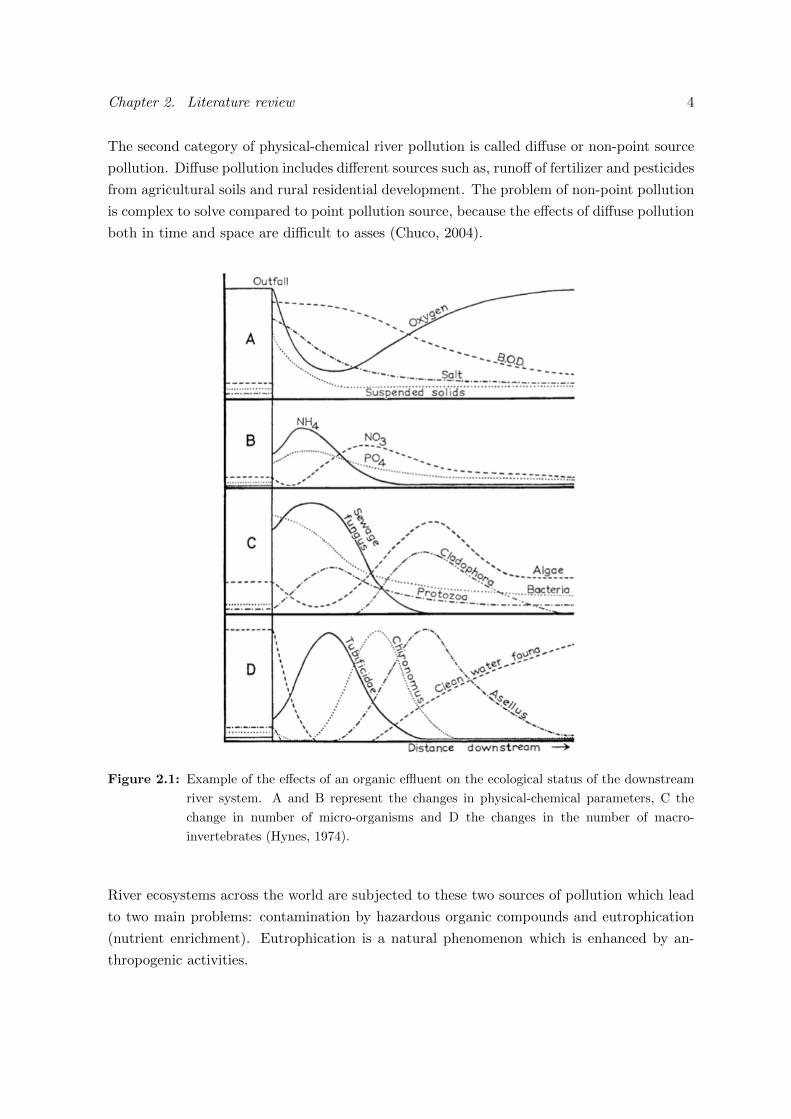
of the ecological system. Hynes (1974) presented one of the best examples related to the
response of ecological systems in function of physical-chemical composition of the river wa-
ter (Figure 2.1). The concentration of different components and the distribution of diverse
organisms like bacteria, fungi, macro-invertebrates are represented in the length profile of
the river. The diagrammatic presentation illustrates the impact of a discharge of pollutants
(e.g. wastewater) on the river system. Physical-chemical river pollution is defined as the
change in physical-chemical parameters of the river due to pollution. Up until 2000, this
train of thought was considered as the core of river water quality assessment, research and
management.
Two categories of physical-chemical river pollution can be distinguished. The first category
is called point source pollution, which is a form of pollution concentrated at one point in
the space. This pollution causes deterioration of the water quality stream downwards of the
pollution point. For example, wastewater is disposed by an industrial facility at a specific
location in the river. This wastewater (WW) can be treated in a wastewater treatment
plant (WWTP) and discharged in the river (controlled discharge) or it can be untreated
and disposed in the river (uncontrolled discharge). Both can attribute substantially to the
deterioration of the physical-chemical water quality downstream of the outlet point.
3
Chapter 2. Literature review 4
The second category of physical-chemical river pollution is called diffuse or non-point source
pollution. Diffuse pollution includes different sources such as, runoff of fertilizer and pesticides
from agricultural soils and rural residential development. The problem of non-point pollution
is complex to solve compared to point pollution source, because the effects of diffuse pollution
both in time and space are difficult to asses (Chuco, 2004).
Figure 2.1: Example of the effects of an organic effluent on the ecological status of the downstream
river system. A and B represent the changes in physical-chemical parameters, C the
change in number of micro-organisms and D the changes in the number of macro-
invertebrates (Hynes, 1974).
River ecosystems across the world are subjected to these two sources of pollution which lead
to two main problems: contamination by hazardous organic compounds and eutrophication
(nutrient enrichment). Eutrophication is a natural phenomenon which is enhanced by an-
thropogenic activities.
Chapter 2. Literature review 5
Runoff from agricultural activities generates an increase of phosphorus and nitrogen (also
called nutrients) in river systems. Wastewater discharge of industries and municipal com-
munities can also increase nutrient concentrations in water bodies. Nutrient enrichment in
combination with light, can cause excessive bloom of algae. This excessive growth of al-
gae can cause large fluctuations in the concentration of dissolved oxygen and can induce an
in-equilibrium in the carbon balance. A decrease in the water quality represented by these
physical-chemical parameters will likely lead to loss in diversity of aquatic organisms and a
disturbance in the ecosystem functioning (Laws, 2000). This is just one of the examples of
the impacts of changing water quality. Most processes in rivers are highly linked to each other
and the change of one parameter can lead to in-balance of many other quality parameters.
This domino-effect can lead to an irreversible deteriorated state of the river water.
Concerning ecological responses to changes in environmental variables, during the last 10
years the emphasis shifted from physical-chemical parameters to habitat quality parameters
(Gabriels et al., 2007; Everaert et al., 2010; Bockelmann et al., 2004). There is a gradu-
ally growing awareness that habitat variables, linked to the hydro-morphologic structure of
the river play an import role in the ecological functioning of rivers and other (regulated)
waterbody systems Timm et al. (2011). This growing awareness of the importance of hydro-
morphology and habitat quality is mainly driven by the European Water Framework Directive
legislation (EWFD, 2000/60/EC), which aims for a “good ecological status” of all water bod-
ies in all European member states by 2015 (European Commission, 2000).
The term “hydro-morphology” is relativity new and has a wide spectrum of definition. Some
definitions are available in the literature, but none of them are used widespread, which makes
the definition a subject for debate. The EWFD defines hydro-morphology as “the hydrological
and geomorphological elements and processes of waterbody systems.”. Orr et al. (2008) and
Newson & Large (2006) define hydro-morphology as the physical habitat formed by the alter-
ing flow regime (hydrology and hydraulics) and the physical structure of the river boundary
(fluvial geomorphology) (Vogel, 2011). Sipek et al. (2010) do not define hydro-morphology,
but do imply its meaning as an overlap of the disciplines of hydrology, (geo)morphology and
ecology. This is an interesting point of view to approach the discussion of interdisciplinary.
Newson et al. (2012) and Vaughan et al. (2009) point out the lack of interdisciplinary and the
integration of the disciplines ecology, (geo)morphology and hydrology. Kilsby et al. (2006)
makes a great attempt to map the interdisciplinary approach by integrating the structural
(hydrology), compositional (geomorphology) and functional (ecology) component which re-
sults in tree specific fields: hydro-morphology, hydroecology and biogeomorphology.
Chapter 2. Literature review 6
Improving monitoring and assessment of the habitat variables linked to the hydro-morphology
must to evolve in river science and management, even though results are lingering (Newson
et al., 2012). Examples of linking habitat variables to ecological responses can be found in
the discipline of eco-hydraulics, where mostly macro-invertebrate occurrence and community
distribution (the “eco-”) is linked to hydraulic variables (the “hydraulics”), like flow velocity,
water height, etc... The composition of the macro-invertebrate community is often linked
to parameters associated with stream hydraulics (Newson et al., 2012; Kemp et al., 2000;
Statzner & Higler, 1986). Earlier, Ward & Stanford (1979) identified temperature, flow
and substrate conditions as the major controlling factors for macro-invertebrate species in
unpolluted river systems. Statzner et al. (1988) implies that more complex hydraulic variables
should be used, on top of the simple variables such as water depth and velocity. Statzner
& Higler (1986) suggests that measurements of current velocity, depth, substrate roughness,
surface slope and hydraulic radius should be used in future hydraulic studies applied to
benthic invertebrates. Furthermore, efforts are done to establish an index which assesses
the hydro-morphological quality in function of the several macro-invertebrate species (Kaeiro
et al., 2011; Extence et al., 1999).
2.2 Modelling water movement and pollutant transport:
water quality models
Water quality models are simulation tools which try to describe the physical, chemical and
biological processes in water ecosystems by means of mathematical equations. The models
offer a framework for integration of diverse physical, chemical and biological information.
The modelling practice aims to provide insight in the river natural processes and serve as a
backbone (background) for decision making in water management Chapra (1997). Following
text will briefly explain some basic concepts of water quality modelling, followed by some
examples of water quality models.
2.2.1 Modelling water movement: flow routing
The first step in water quality modelling is the description of the water movement, also
referred as flow routing. Modelling of water movement or flow routing, in its broad sense
can be considered as the analysis of tracing water flow through a hydrologic system, given a
certain input to the system. Routing methods, which translate the routing in mathematical
equations are divided in two system routing techniques: lumped and distributed. Lumped
system routing is also called hydrologic routing, while distributed system routing is referred
as hydraulic routing. (Chow, 1981).
Chapter 2. Literature review 7
Complex hydraulic routing
In general, the hydraulic routing method describes the routing of water through a channel
bed by solving the “de Saint-Venant” equations (St. Venant) (Barre de Saint-Venant, 1871).
The St. Venant equations are a set of two equations based on the mass and momentum
conservation principle.
The continuity or mass balance equation:
∂Q
∂x+∂Across∂t
= q (2.1)
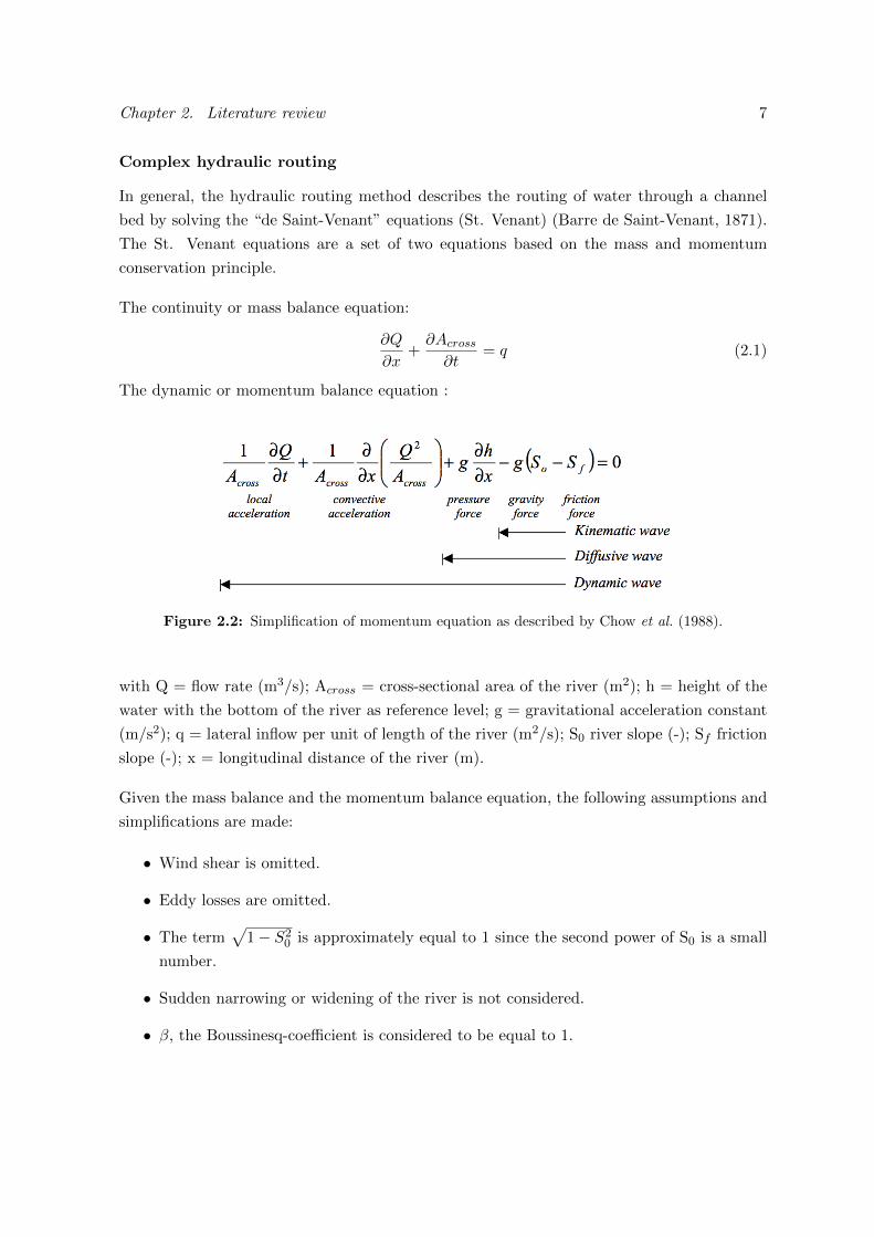
The dynamic or momentum balance equation :
Figure 2.2: Simplification of momentum equation as described by Chow et al. (1988).
with Q = flow rate (m3/s); Across = cross-sectional area of the river (m2); h = height of the
water with the bottom of the river as reference level; g = gravitational acceleration constant
(m/s2); q = lateral inflow per unit of length of the river (m2/s); S0 river slope (-); Sf friction
slope (-); x = longitudinal distance of the river (m).
Given the mass balance and the momentum balance equation, the following assumptions and
simplifications are made:
• Wind shear is omitted.
• Eddy losses are omitted.
• The term√
1 − S20 is approximately equal to 1 since the second power of S0 is a small
number.
• Sudden narrowing or widening of the river is not considered.
• β, the Boussinesq-coefficient is considered to be equal to 1.
Chapter 2. Literature review 8
The full St. Venant equations are rarely solved in water quality modelling practices because
the solution of the equations tends to be complex and require a lot of computational calcula-
tion time. That is why Chow (1981) suggested simplification to the equations. The kinematic
approach only considers friction and gravity forces, resp. Sf and S0 and drops the pressure
and acceleration terms, suggesting that the energy line of the water is parallel to the river
slope. In this case the flow is steady and uniform. When pressure forces become important
but inertial forces remain unimportant, a diffusion wave model can be applied. Both the
kinematic and dynamic wave solution are only able to model stream downward propagation
of a flood wave and can therefore not be used to model stream upwards propagation of waves
in case of backwater effects and mild slopes (S0 < 0.0001 m/m). The dynamic wave solution is
able to describe the propagation of dynamic waves in the downstream and upstream direction
of the river and can therefore be used for modelling of water movement in case of mild slopes
and backwater effects. The acceleration terms in the momentum equation rarely play a role
in water quality issues and the typical time scale are amplified by the conversion processes.
Because of these reasons, diffuse and kinematic approaches are mostly applied in river water
quality modelling practices (Rauch et al., 1998).
Hydrologic routing
Conceptual hydraulic routing is based on the continuity equation and an empirical or ana-
lytical relationship between the storage of water in the system (or reservoir) and the outflow.
Nash (1955) assumed that the response of the catchment on an instantaneous rainfall event
can be represented by a series of linear reservoirs. A linear reservoir is a reservoir whose stor-
age S (m3) is linearly related to the output Q (m3/s) by a storage constant k (1/s) (Chow,
1981). For every reservoir equation 2.2 is valid:
dS
dt= I(t) −Q(t) (2.2)
withdS
dt= change in storage capacity of the reservoir during time step dt (m3/s); I(t) =
inflow reservoir (m3/s) on time t; Q(t) = outflow reservoir (m3/s) on time t.
Chapter 2. Literature review 9
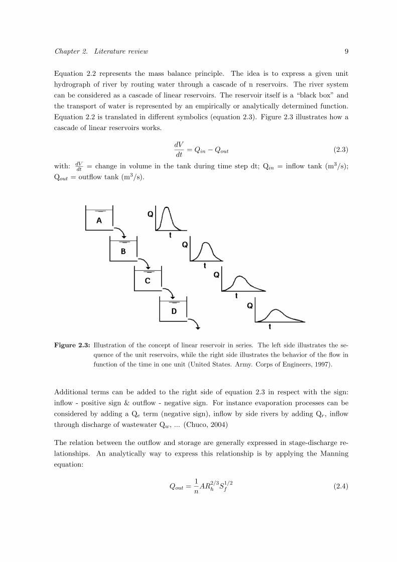
Equation 2.2 represents the mass balance principle. The idea is to express a given unit
hydrograph of river by routing water through a cascade of n reservoirs. The river system
can be considered as a cascade of linear reservoirs. The reservoir itself is a “black box” and
the transport of water is represented by an empirically or analytically determined function.
Equation 2.2 is translated in different symbolics (equation 2.3). Figure 2.3 illustrates how a
cascade of linear reservoirs works.
dV
dt= Qin −Qout (2.3)
with: dVdt = change in volume in the tank during time step dt; Qin = inflow tank (m3/s);
Qout = outflow tank (m3/s).
Figure 2.3: Illustration of the concept of linear reservoir in series. The left side illustrates the se-
quence of the unit reservoirs, while the right side illustrates the behavior of the flow in
function of the time in one unit (United States. Army. Corps of Engineers, 1997).
Additional terms can be added to the right side of equation 2.3 in respect with the sign:
inflow - positive sign & outflow - negative sign. For instance evaporation processes can be
considered by adding a Qe term (negative sign), inflow by side rivers by adding Qr, inflow
through discharge of wastewater Qw, ... (Chuco, 2004)
The relation between the outflow and storage are generally expressed in stage-discharge re-
lationships. An analytically way to express this relationship is by applying the Manning
equation:
Qout =1
nAR
2/3h S
1/2f (2.4)
Chapter 2. Literature review 10
with: Qout = outflow tank (m3/s); n = manning roughness (-); A = cross area (m2); Rh =
hydraulic radius (m2); Sf = friction slope.
Another way to express the relation is to set up an empirical relationship:
Qout = αhβ (2.5)
with α and β two parameters which are determined by calibration of time series of flow and
water height. The concept of representing the river as a cascade of linear reservoir has been
applied by several authors (Benedetti et al., 2007; Deksissa et al., 2004; Kannel et al., 2007)
in water quality modelling and is linked to the concept of continued stirred tank reactors,
which will be explained in the next part of the text.
2.2.2 Modelling pollutant transport: pollutant routing
Pollutant routing deals with the transport of soluble substances in a river. Two types of
deterministic models will be highlighted: the advection-dispersion model and the conceptual
model.
Complex pollutant transport: advection-dispersion model
The advection-dispersion model is based upon the principle of conservation of mass of solutes
and Fick’s diffusion law:
∂C
∂t= [
∂
∂x(Dx
∂C
∂x) +
∂
∂y(Dy
∂C
∂y) +
∂
∂z(Dz
∂C
∂z)] (2.6)
−[∂
∂x(vxC) +
∂
∂y(vyC) +
∂
∂z(vzC)] −R
with C= concentration of pollutant (g/m3); t = time (s); x, y, z = distances in x, y and z
directions (m); ux,y,z = average velocity in the x, y and z direction (m/s); Dx,y,z = Dispersion
coefficients in the x, y and z direction (m2/s); R = reaction transformation rate (g/(m3s).
Equation 2.6 represents the routing of a pollutant in a river in three dimensions. The advection
(second term), diffusion (first term) and reactions (third) term represent the three governing
processes in river systems. Analogues to the St. Venant equations, the equation is rarely
applied in its full form (Rauch et al., 1998).
Chapter 2. Literature review 11
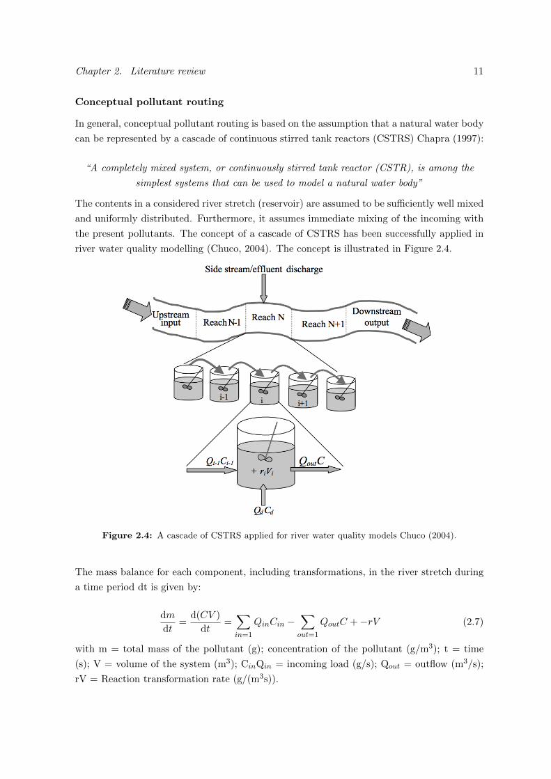
Conceptual pollutant routing
In general, conceptual pollutant routing is based on the assumption that a natural water body
can be represented by a cascade of continuous stirred tank reactors (CSTRS) Chapra (1997):
“A completely mixed system, or continuously stirred tank reactor (CSTR), is among the
simplest systems that can be used to model a natural water body”
The contents in a considered river stretch (reservoir) are assumed to be sufficiently well mixed
and uniformly distributed. Furthermore, it assumes immediate mixing of the incoming with
the present pollutants. The concept of a cascade of CSTRS has been successfully applied in
river water quality modelling (Chuco, 2004). The concept is illustrated in Figure 2.4.
Figure 2.4: A cascade of CSTRS applied for river water quality models Chuco (2004).
The mass balance for each component, including transformations, in the river stretch during
a time period dt is given by:
dm
dt=
d(CV )
dt=
∑in=1
QinCin −∑out=1
QoutC + −rV (2.7)
with m = total mass of the pollutant (g); concentration of the pollutant (g/m3); t = time
(s); V = volume of the system (m3); CinQin = incoming load (g/s); Qout = outflow (m3/s);
rV = Reaction transformation rate (g/(m3s)).
Chapter 2. Literature review 12
2.2.3 Properties and limitations of the use of CSTR in series approach
This section is a short summary of the text presented by Benedetti & Sforzi (1999) and
Reda (1996). The properties of hydraulic modelling with the CSTR scheme is summarized
as followed:
1. Water flows from an upstream reservoir to a downstream reservoir.
2. The mass balance in a tank is only affected by the outflow of the upstream tank.
3. The water surface in every tank is assumed to be constantly horizontal. The change
of water level at the downstream boundary defines a new horizontal water line in the
tank.
4. The outflow is defined by a discharge-rate curve relationship.
The first two properties only assure the downstream propagation of a wave. The most im-
portant limitation of the CSTR in series approach is the lack of upstream propagation of
waves in rivers with a subcritical regime, also called backwater effects. Backwater effects
are effects where the longitudinal water profile (water depth) of the river is affected to a
certain upstream distance. This effect occurs in open channels in a subcritical regime when
a singularity is present at a given cross section. This singularity can be a dam, a submerged
sharp-crest weir or any other structural obstacle or uplift in the river. Furthermore, back-
water effects may also occur in deltaic reaches at a confluence with a big tributary. Lateral
inflow can affect subcritical flow upstream from the discharge point. Also, the downstream
propagation within one single tank is not possible because the water surface in every tank is
assumed to be horizontal. Consequently it is not possible to simulate the slope of the water
in one tank.
2.2.4 A short history lesson in water quality modelling
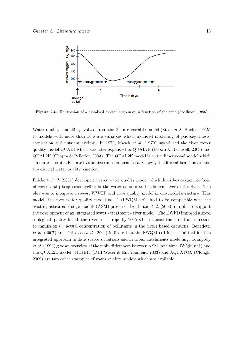
The oxygen sag curve presented by Streeter & Phelps (1925) was the first water quality
model ever presented in literature. The model combines the principles of oxygen demand and
reaeration in order to simulate the effect of pollution through time and space on the dissolved
oxygen in the river. Figure 2.5 shows an illustration of a typical dissolved oxygen sag curve.
In 1960, extended versions of the Streeter-Phelps were introduced.
Chapter 2. Literature review 13
Figure 2.5: Illustration of a dissolved oxygen sag curve in function of the time (Spellman, 1996)
Water quality modelling evolved from the 2 state variable model (Streeter & Phelps, 1925)
to models with more than 10 state variables which included modelling of photosynthesis,
respiration and nutrient cycling. In 1970, Masch et al. (1970) introduced the river water
quality model QUAL1 which was later expanded to QUAL2E (Brown & Barnwell, 2003) and
QUAL2K (Chapra & Pelletier, 2003). The QUAL2K model is a one dimensional model which
simulates the steady state hydraulics (non-uniform, steady flow), the diurnal heat budget and
the diurnal water quality kinetics.
Reichert et al. (2001) developed a river water quality model which describes oxygen, carbon,
nitrogen and phosphorus cycling in the water column and sediment layer of the river. The
idea was to integrate a sewer, WWTP and river quality model in one model structure. This
model, the river water quality model no. 1 (RWQM no1) had to be compatible with the
existing activated sludge models (ASM) presented by Henze et al. (2000) in order to support
the development of an integrated sewer - treatment - river model. The EWFD imposed a good
ecological quality for all the rivers in Europe by 2015 which caused the shift from emission
to immission (= actual concentration of pollutants in the river) based decisions. Benedetti
et al. (2007) and Deksissa et al. (2004) indicate that the RWQM no1 is a useful tool for this
integrated approach in data scarce situations and in urban catchments modelling. Somlyody
et al. (1998) give an overview of the main differences between ASM (and thus RWQM no1) and
the QUAL2E model. MIKE11 (DHI Water & Environment, 2003) and AQUATOX (Clough,
2009) are two other examples of water quality models which are available.
Chapter 2. Literature review 14
2.3 Ecological modelling in an integrated ecological modelling
framework to model biological water quality
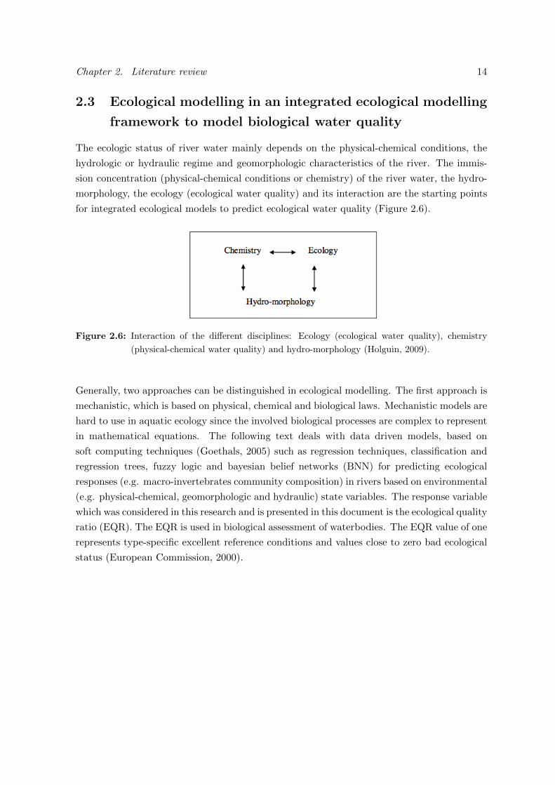
The ecologic status of river water mainly depends on the physical-chemical conditions, the
hydrologic or hydraulic regime and geomorphologic characteristics of the river. The immis-
sion concentration (physical-chemical conditions or chemistry) of the river water, the hydro-
morphology, the ecology (ecological water quality) and its interaction are the starting points
for integrated ecological models to predict ecological water quality (Figure 2.6).
Figure 2.6: Interaction of the different disciplines: Ecology (ecological water quality), chemistry
(physical-chemical water quality) and hydro-morphology (Holguin, 2009).
Generally, two approaches can be distinguished in ecological modelling. The first approach is
mechanistic, which is based on physical, chemical and biological laws. Mechanistic models are
hard to use in aquatic ecology since the involved biological processes are complex to represent
in mathematical equations. The following text deals with data driven models, based on
soft computing techniques (Goethals, 2005) such as regression techniques, classification and
regression trees, fuzzy logic and bayesian belief networks (BNN) for predicting ecological
responses (e.g. macro-invertebrates community composition) in rivers based on environmental
(e.g. physical-chemical, geomorphologic and hydraulic) state variables. The response variable
which was considered in this research and is presented in this document is the ecological quality
ratio (EQR). The EQR is used in biological assessment of waterbodies. The EQR value of one
represents type-specific excellent reference conditions and values close to zero bad ecological
status (European Commission, 2000).
Chapter 2. Literature review 15
2.3.1 Ecological models
This section gives a short overview of the available methods to model ecological water quality
and ecological responses. The author refers to Ahmadi-Nedushan et al. (2006) for an ex-
tended review of the application of these methods. The second part of this text will focus
on some examples of ecological models which are integrated with other type of models (e.g.
water quality models, eco-hydraulic models). These examples serve as indication of current
integrated ecological modelling approaches in (river) aquatic modelling.
Decision trees: classification and regression trees (CART)
The application of classification and regression trees (CART) in ecological modelling is rela-
tively new (O’Brien, 2007). The use of these techniques to predict occurrence, abundance or
biological indices related with macro-invertebrates has gained interest the past years (Ambelu
et al., 2010; Boets et al., 2010; Hoang et al., 2010; Kampichler et al., 2010; Everaert et al.,
2010, 2011). CART, also called decision trees, predict the value of a response variable based
on the value of a set of continuous (regression trees) or discrete (classification trees) predictor
variables. The modelling process follows a recursive method; for every step the most infor-
mative variable is selected as root for a sub-tree. Subsequently, the data set is split up in two
sub data sets. This procedure is continued until a stop criterion is reached.
CART has some unique advantages compared with multivariate statistics. CART is a non-
parametric technique which does not require the specification of a functional form, it is only
based on simple - lower than or greater than - rules. The tree models deal better with non-
linearity and interaction between explanatory variables than other further discussed models
like the ones based on classical or modern regression techniques. Another advantage is the
extreme robustness of these models with respect to outliers (O’Brien, 2007). Besides these
more technical advantages, CART has also some advantage in the field of application in (river
water) management. They provide a very visual and - easy to understand - tool for decision
makers and water managers. Furthermore, classification trees are in particular useful to
develop ecological models in a very short time, and these models are transparent and easy to
interpret (Hoang et al., 2010).
The application of CART has shown to be useful in modelling complex data sets (Breiman
et al., 1984), but as indicated by Goethals (2005), no guidelines exist to support the selection
of learning settings, which makes this method less attractive. Vayssieres et al. (2000) considers
two main problems in constructing an effective decision tree; finding good splits and knowing
when to stop splitting the data set in nodes in order to avoid over-fitting of the data. Besides
the problem of properly pruning, the recursive partitioning method has some disadvantages.
The orthogonal partitioning (perpendicular to the axes) of the data set in the multivariate
space is not always optimal, since it is possible that the optimal split is not defined by solely
Chapter 2. Literature review 16
one variable (one axes). Another disadvantage is the dichotomous structure of the tree, where
later splits are based on fewer cases than the initial split. Small data sets can therefore become
difficult to model with CART (Vayssieres et al., 2000).
Classical regression techniques
Regression methods (analysis) are a denominator for several modelling and analyzing tech-
niques which focus on the relationship between a dependent variable (univariate) and one or
more independent variables (multivariate). In ecology, these models can be used to describe
the relationship between certain species or ecological responses in function of different driv-
ing predictor variables, e.g. water velocity, water temperature, substrate. One of the oldest
and best known regression technique is (multiple) linear regressions; the technique relates a
response variable to one or more independent predictor variables through a linear relation:
Y = β0 + β1x1 + β2x2 + ...+ βmxm + ε (2.8)
with Y = response variable; xi = predictor variable i; βi = regression coefficient i; ε =
error (unexplained variance and measurement error). However, linear regression is limited by
following assumptions:
1. The variance of the errors of the response variable is assumed to be constant (ho-
moscedasticity); they are identically and independently distributed.
2. The errors are assumed to follow a normal Gaussian distribution.
3. The response variable is assumed to respond in a linear relation to predictor variables.
These assumption are mostly not satisfied in modelling ecological responses in function of
environmental variables.
Modern regression techniques
In the case of ecological data sets, it is preferred to use modern regression methods like gen-
eralized linear models (GLMs) and generalized additive models (GAMs) (Ahmadi-Nedushan
et al., 2006) because these techniques can deal with the limitations of classical regression
techniques. GLMs (Nelder & Wedderburn, 1972) are a modern regression tool which are able
to integrate non-normal environmental variables into the models. GAMs are non-parametric
extensions of GLMs which can be applied to data from exponential families of distribu-
tions. The structure of GLM is maintained but the linear predictor of GLM is replaced by a
non-parametric smoothing procedure (smoothing filter) (Guisan et al., 2002; Verrall, 1996).
Generalized linear models are build up from three components; a response variable y, a linear
predictors xi, and the link function g, which describes the functional relationship between the
linear predictors and the expected value of the response variable:
Chapter 2. Literature review 17
g(µ(x)) = β0 + β1x1 + β2x2 + ...+ βmxm (2.9)
The link function is able to describe the many distributions including the normal, binomial,
Poisson, geometric, negative binomial, exponential, and inverse normal distributions (Myers
et al., 2002).
Fuzzy logic
Fuzzy logic is a soft computing technique which uses the fuzzy set theory to include impre-
cise information in a rule-based system by defining adaptable membership functions (Zadeh,
1965). Fuzzy logic can be interpreted as an extension of boolean logic. In boolean logic the
membership of an element to a set is equal to one - the element is a member of the set - or
zero - the element is not a member of the set. In fuzzy logic, an element belongs to the set
with a certain membership value ranging from zero to one. In addition fuzzy logic makes use
of linguistic variables, therefore describing the value of a variable in words. Linguistic if-then
rules are used to describe the relation between the fuzzy input and output. These type of
models can be useful in the field of water quality assessment and structural characteristics
where variables like degree of meandering and substrate type are often difficult to quantify or
classify in a crisp input variable. Furthermore, measurements of physical-chemical variables
characterized by a high uncertainty and temporal variables can also be used a fuzzy input for
these models. However, few fuzzy logic models have been used to support ecosystem man-
agement because of two reasons: the exploration phase in the model development and the
difficulty of convincing managers to use these ’subjective’ models (Goethals, 2005).
Bayesian belief networks
Bayesian belief network models (BBN) are models with a network structure that focus on
the explicit representation of “cause- and-effect” relationships between variables. Bayesian
belief networks consist out of 3 elements (Cain, 2001): a set of nodes representing a discrete
or continuous system variable, a set of links representing causal relationships between nodes
and a set of probabilities, specifying the belief that a node will be in particular state given the
states of the nodes affecting it (parent nodes). The probability distribution in the network
structure makes it possible for the structures to deal with uncertainty and variability in
models. These models are particularly useful in the description of ecological systems, where
cause and effect is a key feature to system dynamics (Regan et al., 2002). The strength of
these model is the “cause-and-effect” relationship integrated in these models; stakeholders
and decision-makers can deliver their input, the decision and furthermore easily understand
the output, the effect of the decision.
Chapter 2. Literature review 18
2.3.2 Integrated ecological models
The water quality models described in section 2.2 are able to cope with predictions of the
physical-chemical water quality and some ecological life forms (e.g. bacteria and algae).
Water quality models are not able to describe all the energy and mass streams in the river
life cycle. As indicated earlier, describing all the physical, chemical and biological laws in
one integrated framework might prove to be difficult. Water quality models cannot describe
the ecological responses expressed in biological water quality. However, integrated ecological
modelling goes further by making a link between physical-chemical, hydro-morphological and
biological aspects of the river system.
Examples of the application of integrated ecological modelling are provided by Tomsic et al.
(2007); Mouton et al. (2007); Holguin & Goethals (2010); Pauwels et al. (2010). Tomsic et al.
(2007) used a habitat suitability index model coupled to a hydrodynamic model (MIKE11)
integrated in an ArcGIS model. A habitat suitability index was set up for both a water
quality sensitive fish and a macro-invertebrate specie (Plecoptera) in order to evaluate the
success of a dam removal for the Sandusky River Ohio. Mouton et al. (2007) presented an
integrated modelling approach by using a fuzzy logic-based eco-hydraulic modelling system.
This modelling system integrated a fish habitat module based on fuzzy logic and a 1 dimen-
sional hydraulic module in order to asses ecological effects of changes in the physical habitat
of the river. The fuzzy approach proved to be a promising method to link different aspects
of the physical structure (hydro-morphology) to the habitat suitability for bullhead (Cottus
gobio L.). Holguin & Goethals (2010) linked the outputs of the water quality model MIKE11
to a GLMs to predict the composition of the macro-invertebrate communities and to asses
the ecological impact of wastewater discharge in a river in Colombia. Pauwels et al. (2010) re-
lated different output variables in the rivers of Flanders, Belgium, of the water quality model
PEGASE (VMM, Flemish environmental agency) to the ecological water quality by using re-
gression trees. Holguin & Goethals (2010) and Pauwels et al. (2010) showed the potential of
integrating water quality and ecological assessment models to evaluate the potential impacts
of the foreseen water quality management plans. Integrated model can function as a powerful
tool in assessing ecological impact of not only wastewater discharge, but also dams and other
impacts.
Chapter 3
Methodology
3.1 Introduction and study area
The Drava river is a cross country river which flows for 750 km from the Italian Alps in
South Tirol to the Donau delta at the Croatian-Serbian border. The Drava river ecosystem
with a catchment area of 40490 km2 is within its category, one of the most preserved river
ecosystems in Europe. The study area of the Drava river ecosystem is located to the north of
the city Varazdin, a city in upper north-east of Croatia (Figure 3.1). The system consists out
of a succession of three lakes called Varazdin, Cakovec and Dubrava. For every lake, a part
of the Drava river is diverted to three succesive hydro-electric power plants (HPP) through
a tailrace canals, while the remaining water is released through the dams in the old Drava
river. The upper boundary of the system is the border of Croatia and Slovenia and the lower
boundary is the end of Dubrava lake. This stretch of 36 km river is considered as one of the
most valuable wetland ecosystems in the Balkan and even Europe. Growing energy demand
in Croatia, during the eighties, initiated the plans for the construction of the three HPP
along this river. Since the construction of the HPP and the dams, this river has functioned
as a multifunctional ecosystem providing different ecosystem services such as recreation (e.g.
fishing), tourism (river viewing), gravel extraction, biodiversity and fresh water provision for
agricultural purposes & hydroelectric production. The human pressure on this ecosystem
is gradually growing because of increased industrialization in the vicinity. Human impacts
include an increased discharge of wastewater and a higher competition between the quantities
of water used for electricity production and ecosystem preservation (Sever et al., 2000).
19
Chapter 3. Methodology 20
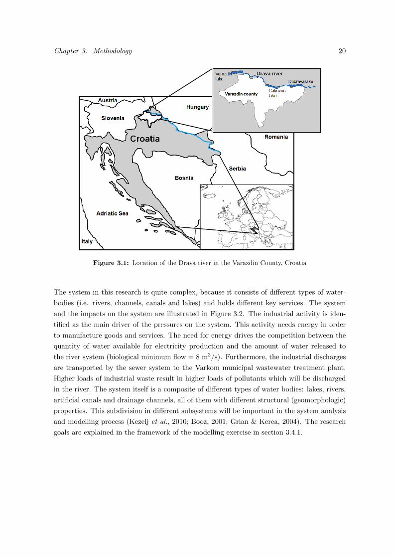
Figure 3.1: Location of the Drava river in the Varazdin County, Croatia
The system in this research is quite complex, because it consists of different types of water-
bodies (i.e. rivers, channels, canals and lakes) and holds different key services. The system
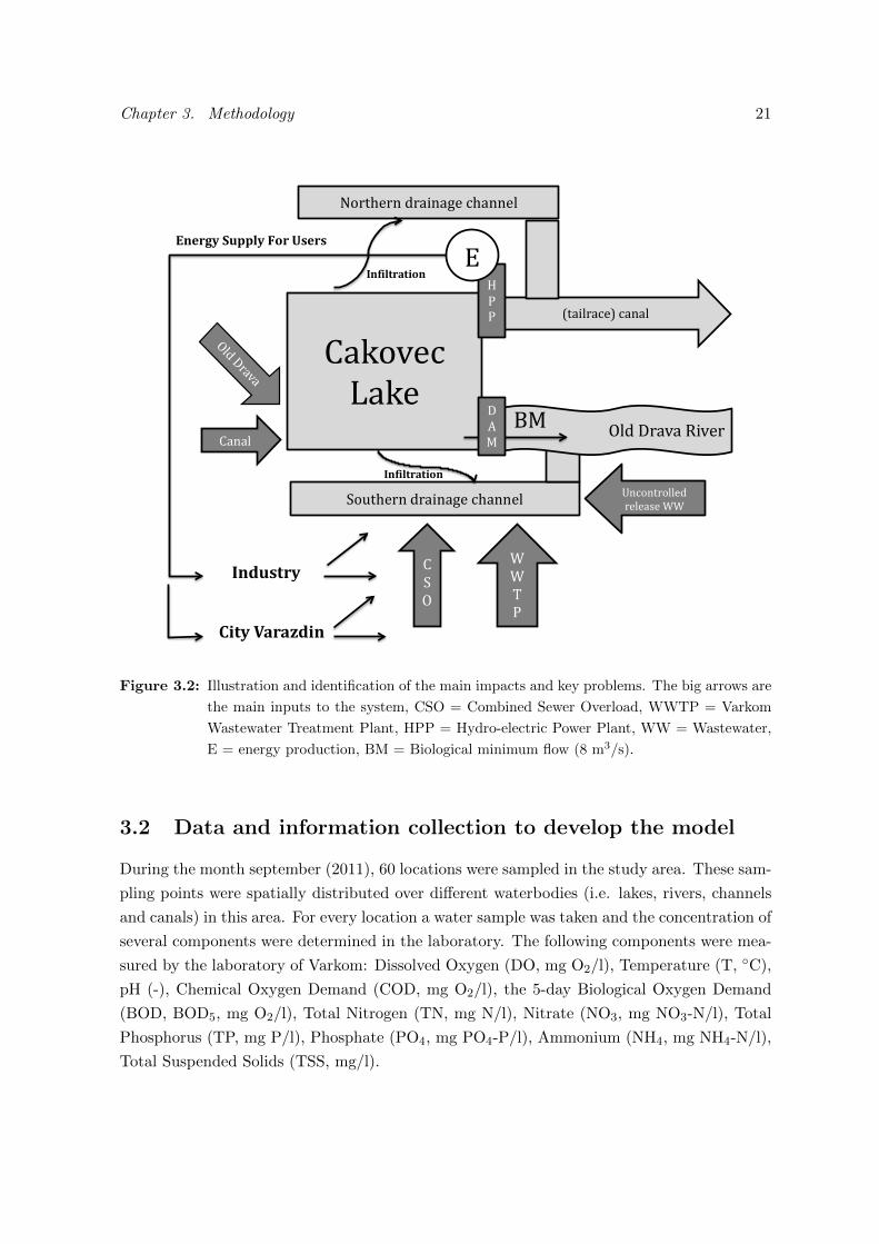
and the impacts on the system are illustrated in Figure 3.2. The industrial activity is iden-
tified as the main driver of the pressures on the system. This activity needs energy in order
to manufacture goods and services. The need for energy drives the competition between the
quantity of water available for electricity production and the amount of water released to
the river system (biological minimum flow = 8 m3/s). Furthermore, the industrial discharges
are transported by the sewer system to the Varkom municipal wastewater treatment plant.
Higher loads of industrial waste result in higher loads of pollutants which will be discharged
in the river. The system itself is a composite of different types of water bodies: lakes, rivers,
artificial canals and drainage channels, all of them with different structural (geomorphologic)
properties. This subdivision in different subsystems will be important in the system analysis
and modelling process (Kezelj et al., 2010; Booz, 2001; Grian & Kerea, 2004). The research
goals are explained in the framework of the modelling exercise in section 3.4.1.
Chapter 3. Methodology 21!
!"#$%&'()!!"#$"%&'()"$$&*
!
!"#$%&'('$)*(+&
!"#$%&#'()*'#+#%
!"#$%&'('
!"#"$
!"#$%&'
!"#$
!"#$"%&$''()*
!"#"$%"&''
!
!
!
!
!
!
!
!
!
!
!"#$%&'!
!"#$%&'(&$)"*
"!
!"#$%&'(')*"+
!"#$%&'()**+&',-$'./#$/'
!"#$%&#'()#*+'*,&(-%*''&.
!
!"#$%&'(&$)"*
!
!
!
#$!
Figure 3.2: Illustration and identification of the main impacts and key problems. The big arrows are
the main inputs to the system, CSO = Combined Sewer Overload, WWTP = Varkom
Wastewater Treatment Plant, HPP = Hydro-electric Power Plant, WW = Wastewater,
E = energy production, BM = Biological minimum flow (8 m3/s).
3.2 Data and information collection to develop the model
During the month september (2011), 60 locations were sampled in the study area. These sam-
pling points were spatially distributed over different waterbodies (i.e. lakes, rivers, channels
and canals) in this area. For every location a water sample was taken and the concentration of
several components were determined in the laboratory. The following components were mea-
sured by the laboratory of Varkom: Dissolved Oxygen (DO, mg O2/l), Temperature (T, ◦C),
pH (-), Chemical Oxygen Demand (COD, mg O2/l), the 5-day Biological Oxygen Demand
(BOD, BOD5, mg O2/l), Total Nitrogen (TN, mg N/l), Nitrate (NO3, mg NO3-N/l), Total
Phosphorus (TP, mg P/l), Phosphate (PO4, mg PO4-P/l), Ammonium (NH4, mg NH4-N/l),
Total Suspended Solids (TSS, mg/l).
Chapter 3. Methodology 22
Macro-invertebrates were sampled by using a hand net and the kick sample method. This
method was performed by walking backwards against the current, where possible, following a
W-shaped path with the hand net (mesh size 250-500 µm). During the sampling procedure,
the person has to kick the bottom layer with his feet and sample just above the river bottom
(or sludge layer). A stretch of 10 to 20 meter was covered by the hand net sampling, this during
3 to 5 minutes, respectively for small and large rivers. At every location, different habitats
(stony areas, deeper stretches, shallower parts) were sampled in order to have a representative
sample for the considered location. Furthermore, stones, branches, leaves of different sizes
were checked and picked out manually. Every sample was examined for the presence of
macro-invertebrates and these organisms were identified up until a specific taxonomical level
as described by De Pauw & Vanhooren (1983). Additional information was collected at every
sampling location by using a field protocol. This information was related to land-use, river
morphology, vegetation, weather conditions and other specific properties of the location.
Historical data was also considered for the data set. Two monitoring campaigns were pre-
formed at in the framework of the project WATROPEC in april and october of 2010, in total
comprehending 46 samples.
3.3 Data exploration and analysis
All the data were processed in the software Matlab (MathWorks, Inc.) and Microsoft Ex-
cel (Microsoft Corporation). The abundance data of every taxa were used to calculate the
Multimetric Macroinvertebrate Index of Flanders (MMIF), a biological index to asses water
quality. The MMIF is a multimetric approach used for the biological assessment of rivers
in Flanders, Belgium, which applies the Ecological Quality Ratio (EQR) approach (Gabriels
et al., 2010). The physical-chemical data and field protocol information were implemented
in a Excel spreadsheet. Derivative data was calculated out of the available data. Organic
nitrogen was calculated assuming that total nitrogen consists of ammonia, nitrate and or-
ganic nitrogen. In the same way, it was assumed that total phosphorus consists of organic
phosphorus and phosphate (Vanrolleghem et al., 2001). A new variable “Type” was defined
which holds information of the hydro-morphologic structure of the waterbody:
1. Hydro-morphological favorable (value 1): natural bank structure, mixed bottom sub-
strate, thin sludge layer, meandering, heterogeneous bank and bottom structure.
2. Hydro-morphological unfavorable (value 2): artificial bank structure, tick sludge layer,
straight waterway, homogeneous bank and bottom structure.
The physical-chemical and biological data were evaluated by comparing the results with data
acquired in 2010 (WATROPEC project). The biological data were evaluated in function of
the habitat variables (chemical properties, river morphology, hydraulics).
Chapter 3. Methodology 23
All the general statistics were calculated: minimum, maximum, mean, median, standard
deviation, 25% and 75% quartiles and the interquartile distance (IQR). The identification of
outliers was performed with three methods: box plots, Cleveland dot plots and mass balance.
Box plots (Box-and-Whisker plots) were set up for the different variables. The box-plots were
only set up for the physical-chemical variables and not for the hydraulic variables. The values
of the upper- and lower-whisker were identified and the points outside the range of these
whiskers were evaluated. Afterwards Cleveland dot plots were used in order to evaluate the
outliers in the data. Cleveland dot plots are plots where the row number of an observation
is plotted vs. the observation value. Cleveland dot plots provide more detailed information
than a box plot. Points that stick out on the right-hand or left-side are observed values
that are considerable larger, or smaller, than the majority of the observations, and require
further investigation (Zuur et al., 2010). A simple mass balance model was set up to check
the physical-chemical data. This model simulates the concentrations of the physical-chemical
variables (BOD, COD, (in-)organic nitrogen and phosphorus, TSS, DO) at every sampling
point in the river given a certain input (= what goes in must come out). Exclusion of a value
from the data set needs to be justified, therefore measured sampling points which do not
coincide with the mass balance models were identified and were tested against the following
questions:
• Were the conditions extreme during the sampling?
• Is there a possible pollutant source near the sampling location?
• Is the value within the range of the values of other sampling campaigns?
• Do the measurement data of the other variables at the sampling location support the
measured value of the parameters? For example, it is highly unlikely that the BOD is
equal to 1 mg O2/l, when the COD is equal to 200 mg O2/l.
• Is there an over- or underestimation of the flow?
• Is the biological data in accordance with the physical-chemical and hydro-morphological
properties?
The data points which do not coincide with the model and where the observed patterns could
not be explained were removed from the data set. The mass balance model was retained to
build the water quality model.
In the last part of the data analysis, two analysis were performed to asses the correlation and
the collinearity between the different predictor variables. A correlation matrix (spearman)
was presented together with a Principal Component Analysis (PCA) of the reduced data
set. This correlation matrix and PCA help to identify the collinearity between the predictor
variables and support the choice of the included variables in the integrated model.
Chapter 3. Methodology 24
3.4 Integrated ecological model building procedure
The following procedure was followed in order to set up an “Integrated Ecological Model”:
1. Clear definition of the problem and the goal of the modelling practice.
2. Framework definition of the considered problem and the model structure.
3. Selection of the model structure.
4. Calibration and validation.
3.4.1 Definition of the problem and goal
As depicted in the introduction of this chapter, the industrial activity is the main driver for
the increasing pressure on this ecosystem. The growing energy demand and emerging poultry,
detergent and milk industry in Varazdin county are leading to an increased pressure on the
Drava ecosystem. The last couple of years, the amount of discharged industrial wastewater
has increased, thus increasing the pressure on the municipal wastewater facility. The capacity
of the wastewater treatment plant is reaching its limits, which increases the risk of discharging
more untreated wastewater (Kezelj et al., 2010). A second stakeholder in the problem are
the hydro-electric infrastructures. Hydro-electric power plants (HPP), all over the country,
together ensure the delivery of energy up to 62,6 % of the total energy production in Croatia
(HEP - Transmission System Operator LLC, 2010). The multipurpose hydro-electric projects
are very interesting subject for debate of the “greenness” of this renewable energy source. The
HPP are very efficient in the conversion of kinetic energy to electricity, the operation costs
are very low which makes them very cost efficient. Among provision of electricity, HPP can
support other services: water supply for agriculture (food production), recreation and flood
regulation. HPPs are therefore a very interesting form of renewable energy, but only if their
operation is in balance with the influenced system. The provision of a minimum biological
flow (8 m3/s) to the Drava river should ensure a steady supply of water to the ecosystem in
order to keep the ecological functioning of the system in balance. But as indicated, there is
an increasing competition between water quantity for the old river path and for electricity
production.
The first goal was to develop a framework for integrated ecological modelling that can be ap-
plied to this problem to illustrate the strength and (dis-)advantages of integrated approach.
The integrated ecological modelling framework presented in the following text was build up
from the philosophy used by Chapra (1997). This author compares the quote from “Tales of
the Dervishes” of Shah (1970) to the problem of water quality modelling. The main reason for
this quote was to make readers aware that he wants to visualize “the whole picture”. There-
fore, by presenting an integrated ecological modelling framework, the goal was persuaded
Chapter 3. Methodology 25
to include the major elements of the system (and its impacts). Furthermore, the research
tries to identify the major problems related to integrated ecological modelling, by means of a
modelling example. Following research questions were formulated:
1. What can be a framework for an integrated ecological model?
2. How can the different elements be build up?
3. How is the data handled for these models? Furthermore, how do we use these data for
calibration and validation of these models? (see also section 3.3)
4. What are the advantages and disadvantages of every model element?
5. What are the implications for the study site?
3.4.2 Framework definition
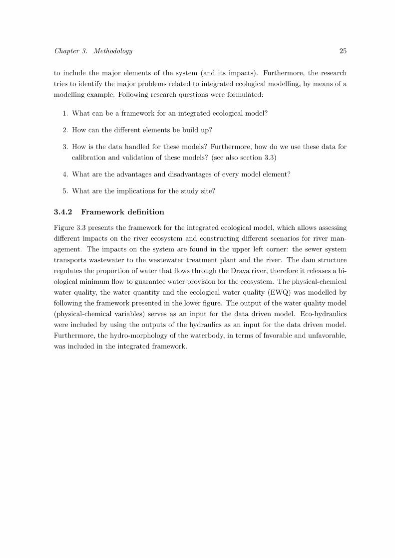
Figure 3.3 presents the framework for the integrated ecological model, which allows assessing
different impacts on the river ecosystem and constructing different scenarios for river man-
agement. The impacts on the system are found in the upper left corner: the sewer system
transports wastewater to the wastewater treatment plant and the river. The dam structure
regulates the proportion of water that flows through the Drava river, therefore it releases a bi-
ological minimum flow to guarantee water provision for the ecosystem. The physical-chemical
water quality, the water quantity and the ecological water quality (EWQ) was modelled by
following the framework presented in the lower figure. The output of the water quality model
(physical-chemical variables) serves as an input for the data driven model. Eco-hydraulics
were included by using the outputs of the hydraulics as an input for the data driven model.
Furthermore, the hydro-morphology of the waterbody, in terms of favorable and unfavorable,
was included in the integrated framework.
Chapter 3. Methodology 26
!
!
Water quantity
Physical-chemical water quality EWQ
IMPACTS
Scenario
analysis
Sewer
WWTP
Dam
Hydro-morphology
Hydraulics
Pollutant transport
WATER
QUALITY
MODEL
DATA
DRIVEN
MODEL!
!"#$%&'()*+,"-.
Hydro-morphology
INTEGRATED ECOLOGICAL MODEL
Figure 3.3: Framework for integrated ecological model, applied to the described problem. EWQ=
Ecological Water Quality, WWTP= Wastewater Treatment Plant
3.4.3 Model structure
Hydraulics: modelling of reservoirs in series
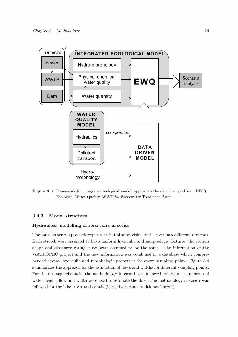
The tanks in series approach requires an initial subdivision of the river into different stretches.
Each stretch were assumed to have uniform hydraulic and morphologic features; the section
shape and discharge rating curve were assumed to be the same. The information of the
WATROPEC project and the new information was combined in a database which compre-
hended several hydraulic and morphologic properties for every sampling point. Figure 3.4
summarizes the approach for the estimation of flows and widths for different sampling points.
For the drainage channels, the methodology in case 1 was followed, where measurements of
water height, flow and width were used to estimate the flow. The methodology in case 2 was
followed for the lake, river and canals (lake, river, canal width not known).
Chapter 3. Methodology 27
The information concerning average flow and water height provided by the Croatian Electric-
ity Company (Hrvatska Elektroprivreda, Sever et al. (2000)) and Grian & Kerea (2004) were
used to estimate the average velocities and widths on several locations. The measured veloc-
ity was used to estimate the width. Since some of the measurements of velocity were at the
border of the waterbody (for instance the lake), the width estimation was biased. Therefore,
the estimated width was compared with the estimated width in the GIS platform ARKOD
available for free consulting by the Croatian Agency for payments in agriculture, fisheries
and rural development (Ministarstvo poljoprivrede, ribarstva i ruralnog razvoja, 2009). The
initial segmentation was based on the segmentation as proposed in the WATROPEC project.
The segments of the river were assumed to have a rectangular cross-section. The length of
every tank was verified with ARKOD and a finer segmentation was proposed for the Drava
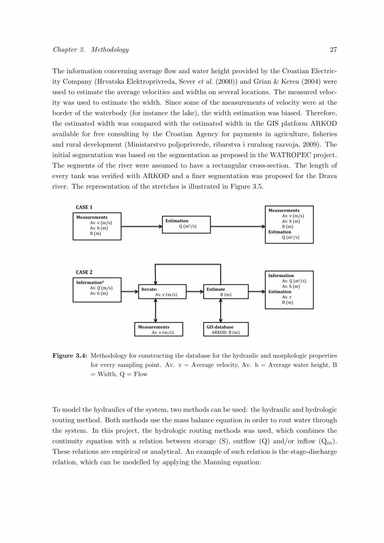
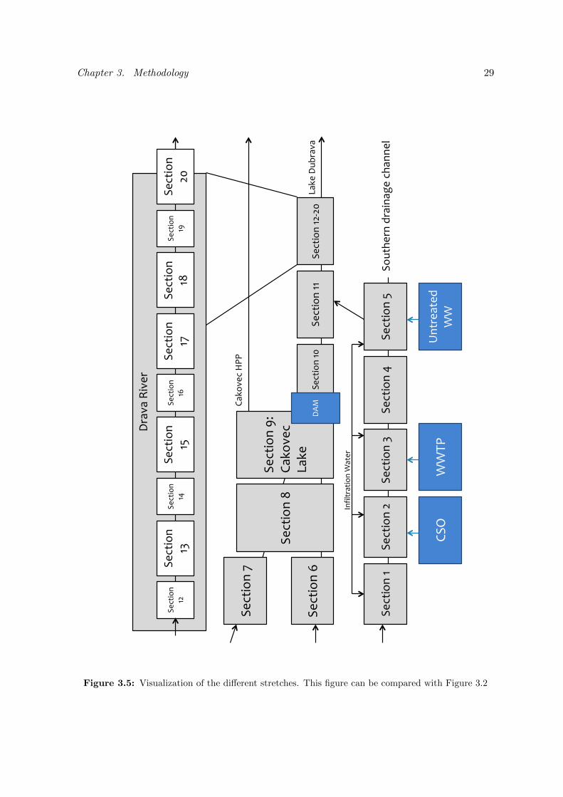
river. The representation of the stretches is illustrated in Figure 3.5.
!
!
!
!
!
!
!
!
!
!
!
!
!
!
!
!
!
!
!
!
!
!
!
!
!
!
!
! !
!"#$%&"'"()$*
"#$!#!%&'()!
"#$!*!%&)!
+!%&)!
!
+$),'#),-(*
,!%&-'()!
!
.(/-&'#),-(0*
"#$!,!%&'()!
"#$!*!%&)!
!
.)"&#)"1!
* "#$!#!%&'()!
+$),'#)"*
+!%&)!
2.3*4#)#5#$"*
!!!!!"./012!+!%&)!
!"#$%&"'"()$*
"#$!#!%&'()!
"#$!*!%&)!
+!%&)!
+$),'#),-(*
,!%&-'()!
!
.(/-&'#),-(*
"#$!,!%&-'()!
"#$!*!%&)!
+$),'#),-(*
* "#$!#!
+!%&)!
!
!"#$%&"'"()$!
* "#$!#!%&'()!
673+*8*
673+*9*
Figure 3.4: Methodology for constructing the database for the hydraulic and morphologic properties
for every sampling point. Av. v = Average velocity, Av. h = Average water height, B
= Width, Q = Flow
To model the hydraulics of the system, two methods can be used: the hydraulic and hydrologic
routing method. Both methods use the mass balance equation in order to rout water through
the system. In this project, the hydrologic routing methods was used, which combines the
continuity equation with a relation between storage (S), outflow (Q) and/or inflow (Qin).
These relations are empirical or analytical. An example of such relation is the stage-discharge
relation, which can be modelled by applying the Manning equation:
Chapter 3. Methodology 28
Q =1
nAcrossR
2/3h S
1/2f (3.1)
with: Q = flow rate (m3/s); n = manning roughness coefficient (-); Across = cross-sectional
area of the river (m2); Rh = Hydraulic radius (Across/P) (m); P = wet perimeter (m); Sf =
friction slope (-).
It was assumed that the conditions of uniform steady flow were valid. The friction slope (or
slope of the water) was assumed equal to the slope of the river bed (S0=Sf ). In this approach,
backwater effects were not considered. Equation 3.1 and equation 3.2 were implemented in
Matlab (MathWorks, Inc) in order to model the hydraulics of the system.
dV
dt= Qin −Q (3.2)
In order to help the explanation of the methodology, the results and the discussion, the
stretches defined in Figure 3.5 are shortly explained:
• Stretches 1 till 5 represent the southern drainage channel receiving treated (Varazdin
WWTP) and untreated wastewater.
• Stretches 6 till 9 represent the lake waterbody, with high water levels and significant
backwater effects due to the dam and the hydropower plant.
• Stretches 10 till 20 represent the old trajectory of the Drava river, with deeper and
shallower zones.
Pollutant transport: cascade of continuous stirred tank reactors
The concept of a cascade of continuous stirred tank reactors (CSTR) was used to model the
transport of pollutants through the river bed. In this approach, a water body is represented
as one or more fully mixed tanks (stretches, applying a “box model”, Shanahan et al. (2001)).
In order to model the pollutant routing, the mass balance, for a given finite time period was
set up for every desired pollutant:
dmi
dt=
d(CiV )
dt=
∑in=1
Qin,iCin,i −∑out=1
Qout,iC + −V ri (3.3)
Equation 3.3 was simplified by applying equations 3.4
d(CiV )
dt= V
dCidt
+ CidV
dtdV
dt=
∑in=1Qin,i −
∑out=1Qout,i
(3.4)
Chapter 3. Methodology 29
!
"#$%&'(!)!
"#$%&'(!*!
"#$%&'(!+!
"#$%&'(!,!
"#$%&'(!-!
"#$%&'(!.!
"#$%&'(!/!
"#$%&'(!01!
234'5#$!
634#!
"#$%&'(!)7!
"#$%&'(!))!
"#$%&'(!)*8*7
!
9:353!;&5#:!
"#$%&'(!
)*!
"#$%&'(!
)+!
"#$%&'(!
),!
"#$%&'(!
)<!
"#$%&'(!
)-!
"#$%&'(!
).!
"#$%&'(!
)/!
"#$%&'(!
)0!
"#$%&'(!
*7!
234'5#$!=>>!
634#!9?@:353!
9AB!
2"C!
DDE>!
F(%:#3%#G!
DD!
H(I&J%:3%&'(!D
3%#:!
"#$%&'(!<!
"'?%K#:(!G:3&(3L#!$K3((#J!
Figure 3.5: Visualization of the different stretches. This figure can be compared with Figure 3.2
Chapter 3. Methodology 30
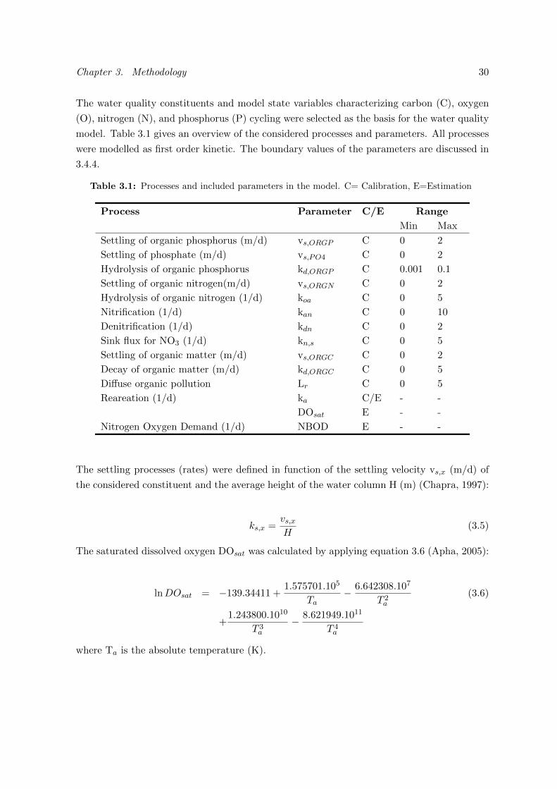
The water quality constituents and model state variables characterizing carbon (C), oxygen
(O), nitrogen (N), and phosphorus (P) cycling were selected as the basis for the water quality
model. Table 3.1 gives an overview of the considered processes and parameters. All processes
were modelled as first order kinetic. The boundary values of the parameters are discussed in
3.4.4.
Table 3.1: Processes and included parameters in the model. C= Calibration, E=Estimation
Process Parameter C/E Range
Min Max
Settling of organic phosphorus (m/d) vs,ORGP C 0 2
Settling of phosphate (m/d) vs,PO4 C 0 2
Hydrolysis of organic phosphorus kd,ORGP C 0.001 0.1
Settling of organic nitrogen(m/d) vs,ORGN C 0 2
Hydrolysis of organic nitrogen (1/d) koa C 0 5
Nitrification (1/d) kan C 0 10
Denitrification (1/d) kdn C 0 2
Sink flux for NO3 (1/d) kn,s C 0 5
Settling of organic matter (m/d) vs,ORGC C 0 2
Decay of organic matter (m/d) kd,ORGC C 0 5
Diffuse organic pollution Lr C 0 5
Reareation (1/d) ka C/E - -
DOsat E - -
Nitrogen Oxygen Demand (1/d) NBOD E - -
The settling processes (rates) were defined in function of the settling velocity vs,x (m/d) of
the considered constituent and the average height of the water column H (m) (Chapra, 1997):
ks,x =vs,xH
(3.5)
The saturated dissolved oxygen DOsat was calculated by applying equation 3.6 (Apha, 2005):
lnDOsat = −139.34411 +1.575701.105
Ta− 6.642308.107
T 2a
(3.6)
+1.243800.1010
T 3a
− 8.621949.1011
T 4a
where Ta is the absolute temperature (K).
Chapter 3. Methodology 31
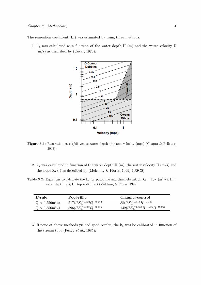
The reareation coefficient (ka) was estimated by using three methods:
1. ka was calculated as a function of the water depth H (m) and the water velocity U
(m/s) as described by (Covar, 1976):
Figure 3.6: Reaeration rate (/d) versus water depth (m) and velocity (mps) (Chapra & Pelletier,
2003).
2. ka was calculated in function of the water depth H (m), the water velocity U (m/s) and
the slope S0 (-) as described by (Melching & Flores, 1999) (USGS):
Table 3.2: Equations to calculate the ka for pool-riffle and channel-control. Q = flow (m3/s), H =
water depth (m), B=top width (m) (Melching & Flores, 1999)
If-rule Pool-riffle Channel-control
Q < 0.556m3/s 517(US0)0.524Q−0.242 88(US0)
0.313H−0.353
Q > 0.556m3/s 596(US0)0.528Q−0.136 142(US0)
0.333H−0.66B−0.243
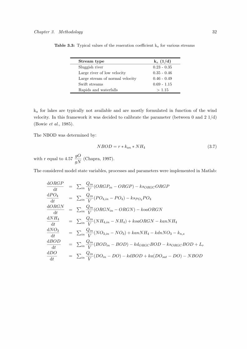
3. If none of above methods yielded good results, the ka was be calibrated in function of
the stream type (Peavy et al., 1985):
Chapter 3. Methodology 32
Table 3.3: Typical values of the reaeration coefficient ka for various streams
Stream type ka (1/d)
Sluggish river 0.23 - 0.35
Large river of low velocity 0.35 - 0.46
Large stream of normal velocity 0.46 - 0.49
Swift streams 0.69 - 1.15
Rapids and waterfalls > 1.15
ka for lakes are typically not available and are mostly formulated in function of the wind
velocity. In this framework it was decided to calibrate the parameter (between 0 and 2 1/d)
(Bowie et al., 1985).
The NBOD was determined by:
NBOD = r ∗ kan ∗NH4 (3.7)
with r equal to 4.57gO
gN(Chapra, 1997).
The considered model state variables, processes and parameters were implemented in Matlab:
dORGP
dt=
∑in
QinV
(ORGPin −ORGP ) − ksORGCORGP
dPO4
dt=
∑in
QinV
(PO4,in − PO4) − ksPO4PO4
dORGN
dt=
∑in
QinV
(ORGNin −ORGN) − koaORGN
dNH4
dt=
∑in
QinV
(NH4,in −NH4) + koaORGN − kanNH4
dNO3
dt=
∑in
QinV
(NO3,in −NO3) + kanNH4 − kdnNO3 − kn,s
dBOD
dt=
∑in
QinV
(BODin −BOD) − kdORGCBOD − ksORGCBOD + Lr
dDO
dt=
∑in
QinV
(DOin −DO) − kdBOD + ka(DOsat −DO) −NBOD
Chapter 3. Methodology 33
In order to summarize, the following processes were considered:
• Settling processes of organic phosphorus, organic nitrogen, phosphate and organic mat-
ter.
• Hydrolysis of organic nitrogen, nitrification and a flux of nitrates to a sink.
• Hydrolysis of organic phosphorus.
• Decay of organic matter.
• Denitrification, diffuse pollution and infiltration water (infiltrated water of the lake) in
the southern drainage channel (Figure 3.2)
• Reaeration
The following processes or variables were not considered:
• Interactions between sediment layer and water column.
• Algae and bacteria growth.
• Total suspended solids.
Ecological model: modelling ecological water quality with regression trees
All the elements discussed in the previous text were integrated in one final model structure.
The model consists of a module which links the physical-chemical, the hydraulic and hydro-
morphological variables in order to model the EWQ. The modelled response variable will was
the MMIF. Regression trees models (RT) were used in order to model the MMIF index. The
advantages of RT are summarized:
• RT are a non-parametric technique which can use information of variables on different
levels of the tree.
• RT are able to integrate interactions which can be missed in multiple regression tech-
niques.
• RT are able to model discrete response variables (MMIF) in function of continues pre-
dictor variables.
• RT deliver a visual result, which can be used by river managers.
• Model development is quick, which makes it possible to generate multiple trees in a
short time span.
The M5’ (Quinlan, 1992; Wang & Witten, 1997) method in the statistical toolbox of Matlab
was used for the tree construction.
Chapter 3. Methodology 34
3.4.4 Calibration & validation
Hydraulic calibration
The calibration of the hydraulic model was based on a manual calibration of two parameters:
the manning roughness n (-) of the river bed and the slope of the river S0 (-). Based on
the available information, initial conditions were proposed for the manning roughness and
the slope. The initial manning coefficient for every stretch was estimated by using a table of
the manning roughness coefficient which describes the roughness in function of the material
or structure of the river bed (Chow et al., 1988; Verhoest, 2010). The slope was initialized
by assuming a research area with a uniform slope. The slope was varied in a range of the
initial slope and boundary values. The slope and roughness was adjusted in function of the
simulations and measurements of the flow and water height of the considered stretch. The
calibration was objectified by taking the difference between the estimated and the modelled
uniform steady-state flow and water height.
Water quality: Monte Carlo calibration
The process parameters of the water quality model were calibrated by preforming a Monte
Carlo analysis. The parameters in the model were considered as a degree of freedom each
bound by a lower and upper boundary value. The boundaries for every parameter are pre-
sented in Table 3.1 and are the boundaries proposed by Garcıa et al. (submitted); Park & Lee
(2002); Chapra (1997). The distribution of these parameters was assumed to be uniform. The
parameters were equal for every stretch in function of the type of water body (the drainage
channel, the river and the lake). For the every run, therefore every set of parameters, the
performance of the model was determined by calculating the root mean square error (RMSE)
between the simulations and the measurements. The errors of the different variables were
assumed not to be equal, thus a weighted sum of least squares (= dividing RMSE of the vari-
able by the measurement variance of the variable) was used in order to evaluated parameters
based on two or more variables. In order to evaluate the calibration, the spearman correlation
coefficient r and the coefficient of determination R2 (1-SSE/SST) were used. The model was
calibrated separately for:
• The southern drainage channel with inputs of the combined sewer overload, the wastew-
ater treatment plant and inputs of untreated wastewater;
• The Drava river (succession river-lake-river) with inputs of the Varazdin tailrace canal
and the southern drainage channel.
If the results for the automatic calibration were not satisfying, then manual fine tuning was
performed. The Monte Carlo analysis was performed to indicate the variability of the variable
values in function of the chosen parameters. The model was calibrated with the data of the
Chapter 3. Methodology 35
third sampling campaign, the validation was done with the second sampling campaign. The
model could not be validated for the first monitoring campaign since not enough input data
was available.
Training and validation of the regression trees
The tree training and validation was focused on finding the optimal tree, which satisfied several
performance criteria and provided ecological relevant results (Goethals, 2005). As mentioned
in the introduction, the training and validation requires the interaction of the user and might
be prone to subjectivity; selection of the tree size, selection of the ecological relevant tree.
The validation was based upon three types of validation as proposed by Goethals (2005):
1. Theoretical validation with correctly classified instances (CCI), regression coefficient
(r), coefficient of determination (R2=1-SSE
SST) and root mean square error (RMSE).
2. Validation by testing the tree to ecological knowledge.
3. Validation by practical use of the model.
The first two criteria were used for the validation of the regression tree. Two different ap-
proaches were used to build up the regression tree.
In the first part, the data sets of every sampling campaign were used to train the tree and
independently validate the tree. For this purpose, the data of sampling campaign 3 was used
for the training and the data of sampling campaign 1 and 2 was used for the validation.
This action was repeated for total the data set (with outliers!), the data set without outliers
identified with the Cleveland dot plots and the data set without outliers identified by the
Cleveland dot plots and mass balance model, therefore creating in total three models, which
could be compared in performance. In order to quantify the performance of the calibration
and validation the CCI, RMSE, r and R2 were calculated. These values were compared with
the average values of the performance criteria tested with a model which generates a random
class of EWQ (e.g. bad, poor, moderate, good). These values were generated by randomly
picking a MMIF class for all data points, then calculating the performance indices between
the randomly picked classes and the measured classes in order to repeat this procedure a 1000
times to calculate the average values of the performance indices of the 1000 random models.
Furthermore, in the second part, a bootstrapping approach was implemented to compare
performance criteria of different trees. The bootstrap approach is an approach in which a
smaller subsample (child data set) of the available data was used to train and create a model.
Therefore, a child database was used for the tree construction (Sipek et al., 2010; Gibson
et al., 2004). The child data for each of these models was based on stratified runs of the data
sets. A stratified run is run which generates a random stratified data set based on the total
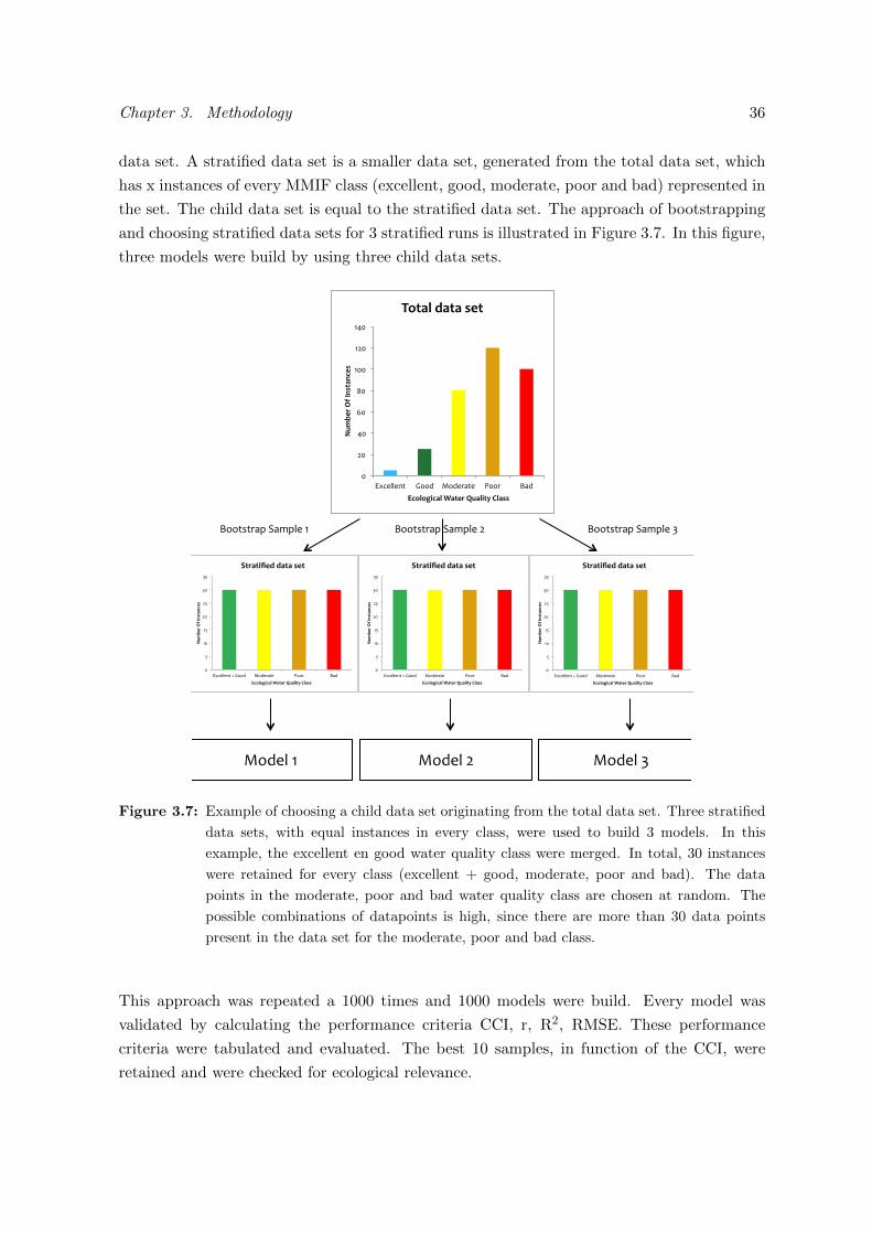
Chapter 3. Methodology 36
data set. A stratified data set is a smaller data set, generated from the total data set, which
has x instances of every MMIF class (excellent, good, moderate, poor and bad) represented in
the set. The child data set is equal to the stratified data set. The approach of bootstrapping
and choosing stratified data sets for 3 stratified runs is illustrated in Figure 3.7. In this figure,
three models were build by using three child data sets.
!!
!
!
!
!"
#!"
$!"
%!"
&!"
'!!"
'#!"
'$!"
()*+,,+-." /001" 201+34.+" 5003" 641"
!"#$%&'()'*+,-.+/%
,'
0/12134/.2'5.-%&'6".24-7'82.,,'
91-.2':.-.',%-'
!"
#"
$!"
$#"
%!"
%#"
&!"
&#"
'()*++*,-"."/001" 201*34-*" 5003" 641"
!"#$%&'()'*+,-.+/%
,'
0/12134/.2'5.-%&'6".24-7'82.,,'
9-&.-4:%;';.-.',%-'
!"
#"
$!"
$#"
%!"
%#"
&!"
&#"
'()*++*,-"."/001" 201*34-*" 5003" 641"
!"#$%&'()'*+,-.+/%
,'
0/12134/.2'5.-%&'6".24-7'82.,,'
9-&.-4:%;';.-.',%-'
!"
#"
$!"
$#"
%!"
%#"
&!"
&#"
'()*++*,-"."/001" 201*34-*" 5003" 641"
!"#$%&'()'*+,-.+/%
,'
0/12134/.2'5.-%&'6".24-7'82.,,'
9-&.-4:%;';.-.',%-'
"#$%&!'! "#$%&!(! "#$%&!)!
*##+,+-./!0.1/&%!'! *##+,+-./!0.1/&%!(! *##+,+-./!0.1/&%!)!
Figure 3.7: Example of choosing a child data set originating from the total data set. Three stratified
data sets, with equal instances in every class, were used to build 3 models. In this
example, the excellent en good water quality class were merged. In total, 30 instances
were retained for every class (excellent + good, moderate, poor and bad). The data
points in the moderate, poor and bad water quality class are chosen at random. The
possible combinations of datapoints is high, since there are more than 30 data points
present in the data set for the moderate, poor and bad class.
This approach was repeated a 1000 times and 1000 models were build. Every model was
validated by calculating the performance criteria CCI, r, R2, RMSE. These performance
criteria were tabulated and evaluated. The best 10 samples, in function of the CCI, were
retained and were checked for ecological relevance.
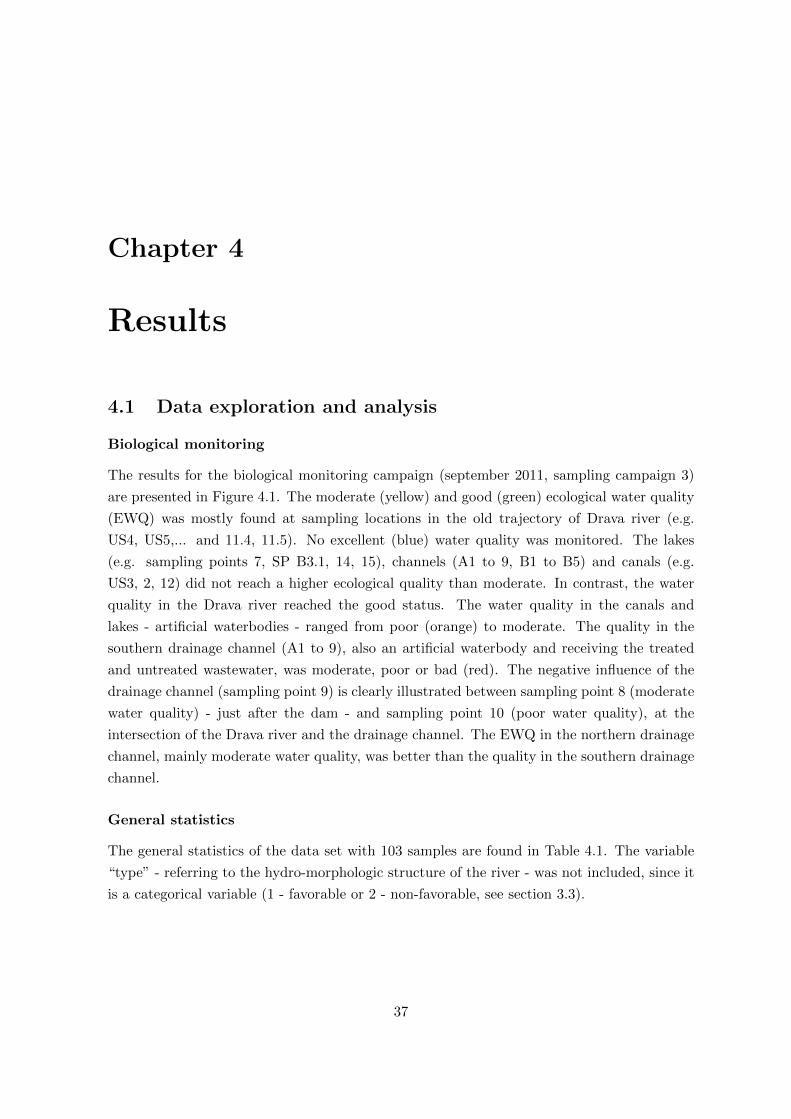
Chapter 4
Results
4.1 Data exploration and analysis
Biological monitoring
The results for the biological monitoring campaign (september 2011, sampling campaign 3)
are presented in Figure 4.1. The moderate (yellow) and good (green) ecological water quality
(EWQ) was mostly found at sampling locations in the old trajectory of Drava river (e.g.
US4, US5,... and 11.4, 11.5). No excellent (blue) water quality was monitored. The lakes
(e.g. sampling points 7, SP B3.1, 14, 15), channels (A1 to 9, B1 to B5) and canals (e.g.
US3, 2, 12) did not reach a higher ecological quality than moderate. In contrast, the water
quality in the Drava river reached the good status. The water quality in the canals and
lakes - artificial waterbodies - ranged from poor (orange) to moderate. The quality in the
southern drainage channel (A1 to 9), also an artificial waterbody and receiving the treated
and untreated wastewater, was moderate, poor or bad (red). The negative influence of the
drainage channel (sampling point 9) is clearly illustrated between sampling point 8 (moderate
water quality) - just after the dam - and sampling point 10 (poor water quality), at the
intersection of the Drava river and the drainage channel. The EWQ in the northern drainage
channel, mainly moderate water quality, was better than the quality in the southern drainage
channel.
General statistics
The general statistics of the data set with 103 samples are found in Table 4.1. The variable
“type” - referring to the hydro-morphologic structure of the river - was not included, since it
is a categorical variable (1 - favorable or 2 - non-favorable, see section 3.3).
37
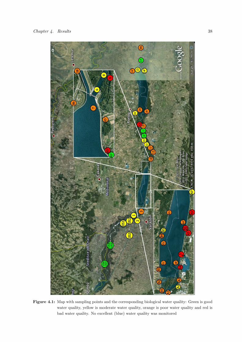
Chapter 4. Results 38
Figure 4.1: Map with sampling points and the corresponding biological water quality: Green is good
water quality, yellow is moderate water quality, orange is poor water quality and red is
bad water quality. No excellent (blue) water quality was monitored
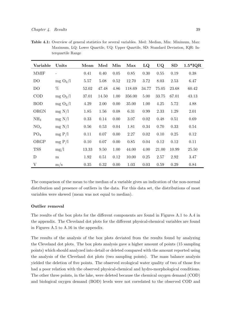
Chapter 4. Results 39
Table 4.1: Overview of general statistics for several variables. Med: Median, Min: Minimum, Max:
Maximum, LQ: Lower Quartile, UQ: Upper Quartile, SD: Standard Deviation, IQR: In-
terquartile Range
Variable Units Mean Med Min Max LQ UQ SD 1.5*IQR
MMIF - 0.41 0.40 0.05 0.85 0.30 0.55 0.19 0.38
DO mg O2/l 5.57 5.08 0.52 12.70 3.72 8.03 2.53 6.47
DO % 52.02 47.48 4.86 118.69 34.77 75.05 23.68 60.42
COD mg O2/l 37.01 14.50 1.00 356.00 5.00 33.75 67.01 43.13
BOD mg O2/l 4.29 2.00 0.00 35.00 1.00 4.25 5.72 4.88
ORGN mg N/l 1.85 1.56 0.08 6.31 0.99 2.33 1.29 2.01
NH4 mg N/l 0.33 0.14 0.00 3.07 0.02 0.48 0.51 0.69
NOx mg N/l 0.56 0.53 0.04 1.81 0.34 0.70 0.33 0.54
PO4 mg P/l 0.11 0.07 0.00 2.27 0.02 0.10 0.25 0.12
ORGP mg P/l 0.10 0.07 0.00 0.85 0.04 0.12 0.12 0.11
TSS mg/l 13.33 9.50 1.00 44.00 4.00 21.00 10.99 25.50
D m 1.92 0.51 0.12 10.00 0.25 2.57 2.92 3.47
V m/s 0.35 0.32 0.00 1.03 0.03 0.59 0.29 0.84
The comparison of the mean to the median of a variable gives an indication of the non-normal
distribution and presence of outliers in the data. For this data set, the distributions of most
variables were skewed (mean was not equal to median).
Outlier removal
The results of the box plots for the different components are found in Figures A.1 to A.4 in
the appendix. The Cleveland dot plots for the different physical-chemical variables are found
in Figures A.5 to A.16 in the appendix.
The results of the analysis of the box plots deviated from the results found by analyzing
the Cleveland dot plots. The box plots analysis gave a higher amount of points (15 sampling
points) which should analyzed into detail or deleted compared with the amount reported using
the analysis of the Cleveland dot plots (two sampling points). The mass balance analysis
yielded the deletion of five points. The observed ecological water quality of two of those five
had a poor relation with the observed physical-chemical and hydro-morphological conditions.
The other three points, in the lake, were deleted because the chemical oxygen demand (COD)
and biological oxygen demand (BOD) levels were not correlated to the observed COD and
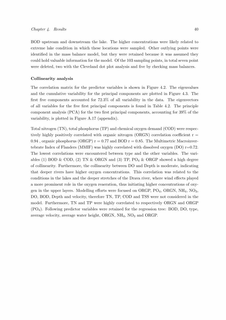
Chapter 4. Results 40
BOD upstream and downstream the lake. The higher concentrations were likely related to
extreme lake condition in which these locations were sampled. Other outlying points were
identified in the mass balance model, but they were retained because it was assumed they
could hold valuable information for the model. Of the 103 sampling points, in total seven point
were deleted, two with the Cleveland dot plot analysis and five by checking mass balances.
Collinearity analysis
The correlation matrix for the predictor variables is shown in Figure 4.2. The eigenvalues
and the cumulative variability for the principal components are plotted in Figure 4.3. The
first five components accounted for 72.3% of all variability in the data. The eigenvectors
of all variables for the five first principal components is found in Table 4.2. The principle
component analysis (PCA) for the two first principal components, accounting for 39% of the
variability, is plotted in Figure A.17 (appendix).
Total nitrogen (TN), total phosphorus (TP) and chemical oxygen demand (COD) were respec-
tively highly positively correlated with organic nitrogen (ORGN) correlation coefficient r =
0.94 , organic phosphorus (ORGP) r = 0.77 and BOD r = 0.85. The Multimetric Macroinver-
tebrate Index of Flanders (MMIF) was highly correlated with dissolved oxygen (DO) r=0.72.
The lowest correlations were encountered between type and the other variables. The vari-
ables (1) BOD & COD, (2) TN & ORGN and (3) TP, PO4 & ORGP showed a high degree
of collinearity. Furthermore, the collinearity between DO and Depth is moderate, indicating
that deeper rivers have higher oxygen concentrations. This correlation was related to the
conditions in the lakes and the deeper stretches of the Drava river, where wind effects played
a more prominent role in the oxygen reaeration, thus initiating higher concentrations of oxy-
gen in the upper layers. Modelling efforts were focused on ORGP, PO4, ORGN, NH4, NO3,
DO, BOD, Depth and velocity, therefore TN, TP, COD and TSS were not considered in the
model. Furthermore, TN and TP were highly correlated to respectively ORGN and ORGP
(PO4). Following predictor variables were retained for the regression tree: BOD, DO, type,
average velocity, average water height, ORGN, NH4, NO3 and ORGP.
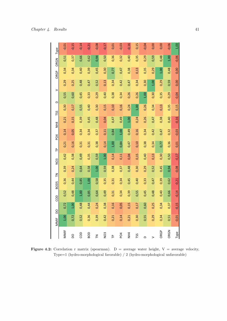
Chapter 4. Results 41
!!"#
$%&
'%$
(%$)
*+
+%,
&*-&
-%.
+/.
*00&
$1
%23-
%23+
*456
!!"#&
7899
98:;
98);
98,<
98,=
98.;
98;7
987.
98;7
98,9
98))
98;=
98,.
98)7
>9897
$%&
98:;
7899
98.?
98..
98;.
98,?
987<
989)
987)
987:
98<9
98;)
98,.
98,:
>987)
'%$
98);
98.?
7899
98?)
98<.
98.=
98,7
98,.
98,=
98))
98.)
98.?
98.9
98<<
>987.
(%$
98,<
98..
98?)
7899
98)?
98,)
98,7
98,.
98.)
98.9
98,,
98.:
98,=
98<;
>98;7
*+
98,=
98;.
98<.
98)?
7899
98)=
98,?
98,:
98.?
98,9
98;=
98);
98.)
98=.
>989?
+%,
98.;
98,?
98.=
98,)
98)=
7899
987.
9877
989.
987)
98.9
987,
98,9
98)9
>987:
*-
98;7
987<
98,7
98,7
98,?
987.
7899
98?.
98.:
9879
98,?
98,.
98::
98,<
9897
-%.
987.
989)
98,.
98,.
98,:
9877
98?.
7899
98.=
987<
98,.
98.;
98.:
98,;
>989,
+/.
98;7
987)
98,=
98.)
98.?
989.
98.:
98.=
7899
98;.
98;<
98.:
98,?
98.9
>987<
*00&
98,9
987:
98))
98.9
98,9
987)
9879
987<
98;.
7899
98;<
98,.
987,
98,)
987)
$98))
98<9
98.)
98,,
98;=
98.9
98,?
98,.
98;<
98;<
7899
98,9
98,)
98;=
>989.
198;=
98;)
98.?
98.:
98);
987,
98,.
98.;
98.:
98,.
98,9
7899
98;=
98)=
9899
%23-
98,.
98,.
98.9
98,=
98.)
98,9
98::
98.:
98,?
987,
98,)
98;=
7899
98.?
9899
%23+
98)7
98,:
98<<
98<;
98=.
98)9
98,<
98,;
98.9
98,)
98;=
98)=
98.?
7899
>989<
*456
>9897
>987)
>987.
>98;7
>989?
>987:
9897
>989,
>987<
987)
>989.
9899
9899
>989<
7899
Figure 4.2: Correlation r matrix (spearman). D = average water height, V = average velocity,
Type=1 (hydro-morphological favorable) / 2 (hydro-morphological unfavorable)
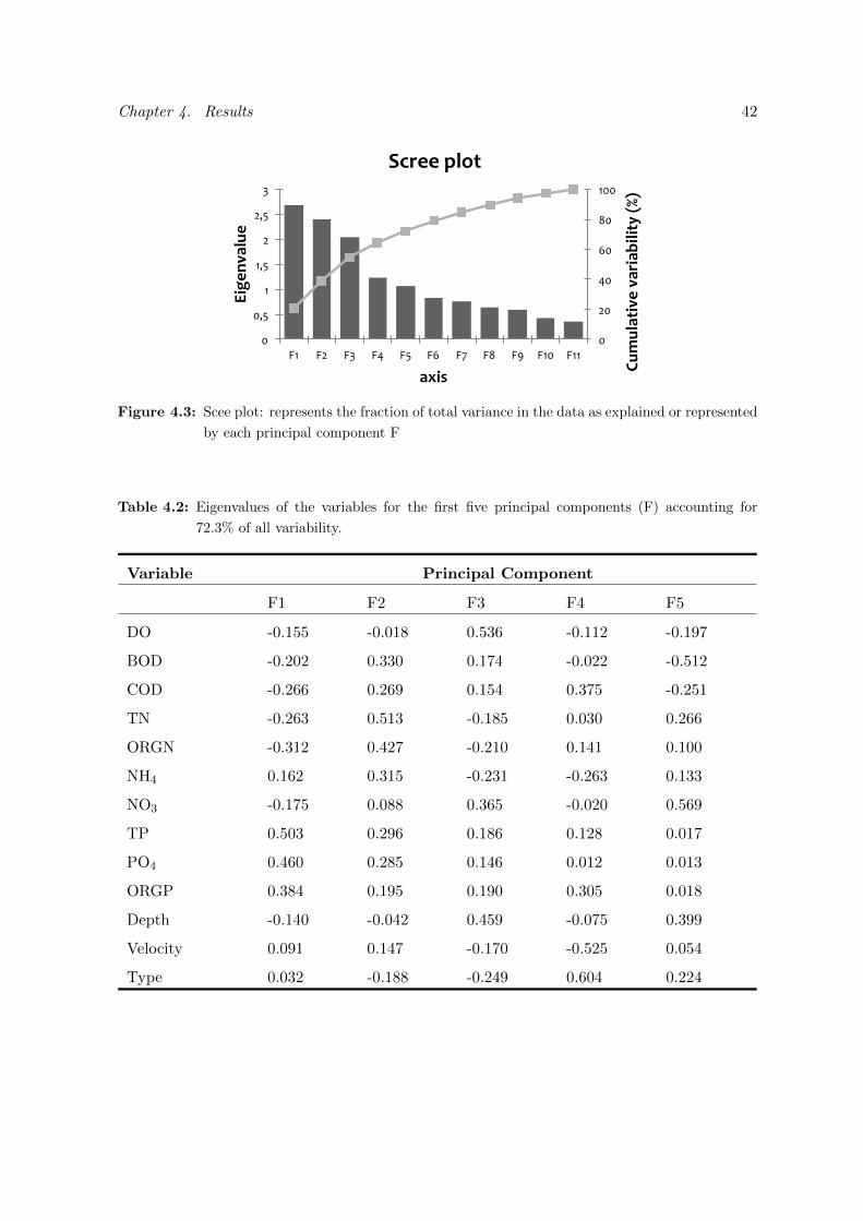
Chapter 4. Results 42
!"
#!"
$!"
%!"
&!"
'!!"
!"
!()"
'"
'()"
#"
#()"
*"
+'" +#" +*" +$" +)" +%" +," +&" +-" +'!" +''"
!"#"$%&'()
*(%+'%,'$'&-*./0*
1'2)3(%
$")*
%4'5*
67+))*8$9&*
Figure 4.3: Scee plot: represents the fraction of total variance in the data as explained or represented
by each principal component F
Table 4.2: Eigenvalues of the variables for the first five principal components (F) accounting for
72.3% of all variability.
Variable Principal Component
F1 F2 F3 F4 F5
DO -0.155 -0.018 0.536 -0.112 -0.197
BOD -0.202 0.330 0.174 -0.022 -0.512
COD -0.266 0.269 0.154 0.375 -0.251
TN -0.263 0.513 -0.185 0.030 0.266
ORGN -0.312 0.427 -0.210 0.141 0.100
NH4 0.162 0.315 -0.231 -0.263 0.133
NO3 -0.175 0.088 0.365 -0.020 0.569
TP 0.503 0.296 0.186 0.128 0.017
PO4 0.460 0.285 0.146 0.012 0.013
ORGP 0.384 0.195 0.190 0.305 0.018
Depth -0.140 -0.042 0.459 -0.075 0.399
Velocity 0.091 0.147 -0.170 -0.525 0.054
Type 0.032 -0.188 -0.249 0.604 0.224
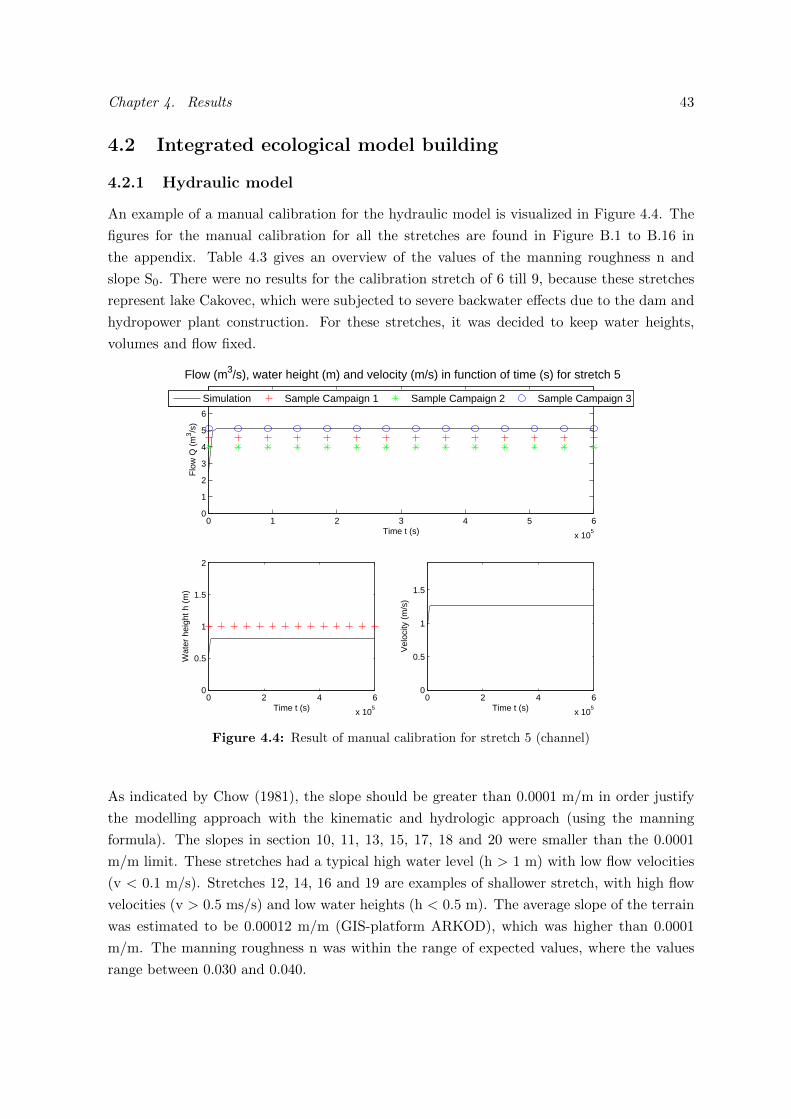
Chapter 4. Results 43
4.2 Integrated ecological model building
4.2.1 Hydraulic model
An example of a manual calibration for the hydraulic model is visualized in Figure 4.4. The
figures for the manual calibration for all the stretches are found in Figure B.1 to B.16 in
the appendix. Table 4.3 gives an overview of the values of the manning roughness n and
slope S0. There were no results for the calibration stretch of 6 till 9, because these stretches
represent lake Cakovec, which were subjected to severe backwater effects due to the dam and
hydropower plant construction. For these stretches, it was decided to keep water heights,
volumes and flow fixed.
0 1 2 3 4 5 6
x 105
0
1
2
3
4
5
6
7
Time t (s)
Flo
w Q
(m
3 /s)
Flow (m3/s), water height (m) and velocity (m/s) in function of time (s) for stretch 5
Simulation Sample Campaign 1 Sample Campaign 2 Sample Campaign 3
0 2 4 6
x 105
0
0.5
1
1.5
2
Wat
er h
eigh
t h (
m)
Time t (s)0 2 4 6
x 105
0
0.5
1
1.5
Vel
ocity
(m
/s)
Time t (s)
Figure 4.4: Result of manual calibration for stretch 5 (channel)
As indicated by Chow (1981), the slope should be greater than 0.0001 m/m in order justify
the modelling approach with the kinematic and hydrologic approach (using the manning
formula). The slopes in section 10, 11, 13, 15, 17, 18 and 20 were smaller than the 0.0001
m/m limit. These stretches had a typical high water level (h > 1 m) with low flow velocities
(v < 0.1 m/s). Stretches 12, 14, 16 and 19 are examples of shallower stretch, with high flow
velocities (v > 0.5 ms/s) and low water heights (h < 0.5 m). The average slope of the terrain
was estimated to be 0.00012 m/m (GIS-platform ARKOD), which was higher than 0.0001
m/m. The manning roughness n was within the range of expected values, where the values
range between 0.030 and 0.040.
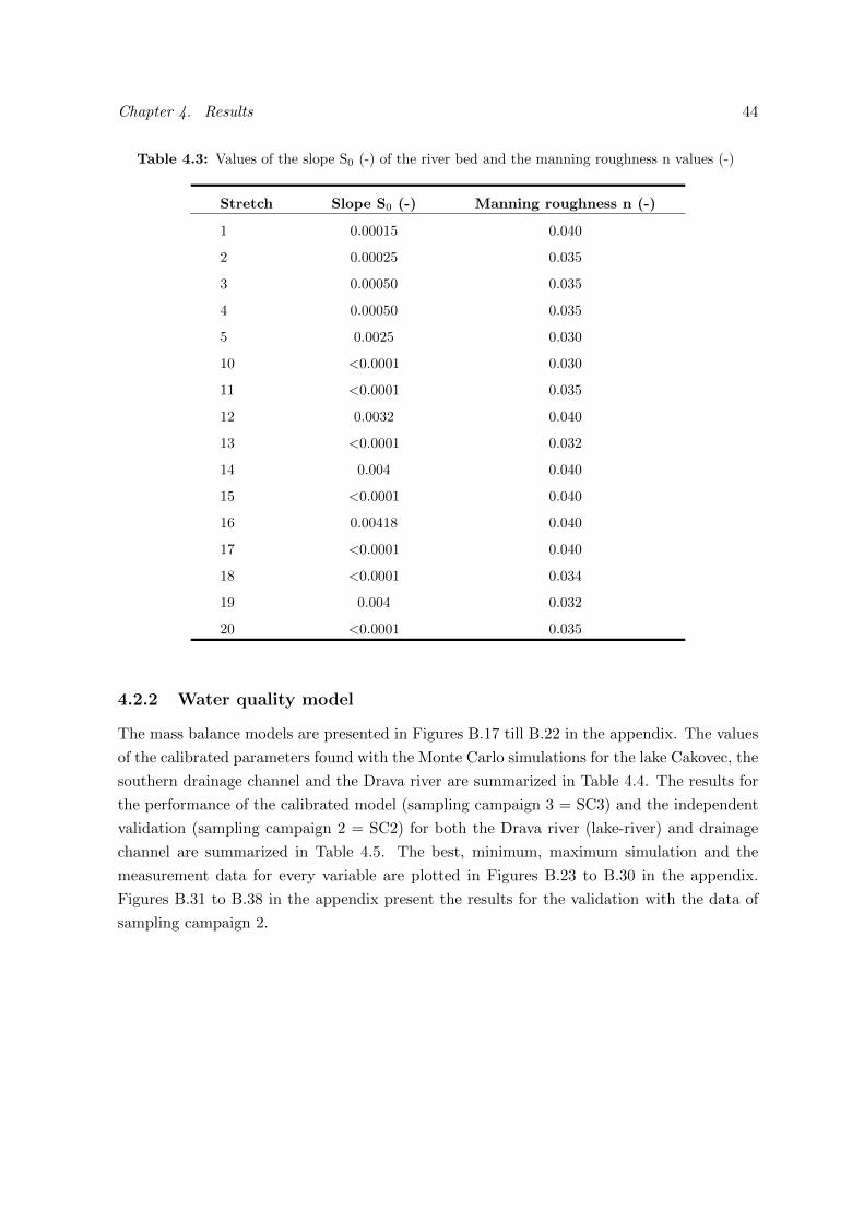
Chapter 4. Results 44
Table 4.3: Values of the slope S0 (-) of the river bed and the manning roughness n values (-)
Stretch Slope S0 (-) Manning roughness n (-)
1 0.00015 0.040
2 0.00025 0.035
3 0.00050 0.035
4 0.00050 0.035
5 0.0025 0.030
10 <0.0001 0.030
11 <0.0001 0.035
12 0.0032 0.040
13 <0.0001 0.032
14 0.004 0.040
15 <0.0001 0.040
16 0.00418 0.040
17 <0.0001 0.040
18 <0.0001 0.034
19 0.004 0.032
20 <0.0001 0.035
4.2.2 Water quality model
The mass balance models are presented in Figures B.17 till B.22 in the appendix. The values
of the calibrated parameters found with the Monte Carlo simulations for the lake Cakovec, the
southern drainage channel and the Drava river are summarized in Table 4.4. The results for
the performance of the calibrated model (sampling campaign 3 = SC3) and the independent
validation (sampling campaign 2 = SC2) for both the Drava river (lake-river) and drainage
channel are summarized in Table 4.5. The best, minimum, maximum simulation and the
measurement data for every variable are plotted in Figures B.23 to B.30 in the appendix.
Figures B.31 to B.38 in the appendix present the results for the validation with the data of
sampling campaign 2.
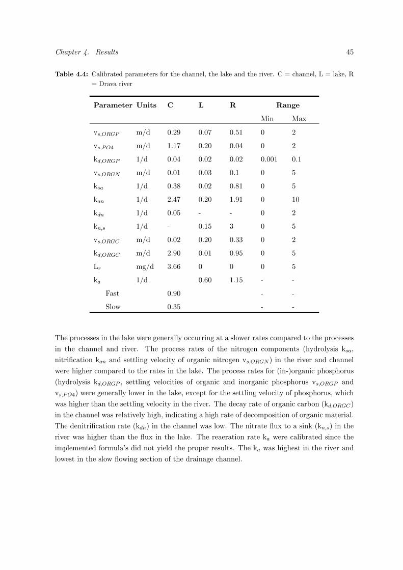
Chapter 4. Results 45
Table 4.4: Calibrated parameters for the channel, the lake and the river. C = channel, L = lake, R
= Drava river
Parameter Units C L R Range
Min Max
vs,ORGP m/d 0.29 0.07 0.51 0 2
vs,PO4 m/d 1.17 0.20 0.04 0 2
kd,ORGP 1/d 0.04 0.02 0.02 0.001 0.1
vs,ORGN m/d 0.01 0.03 0.1 0 5
koa 1/d 0.38 0.02 0.81 0 5
kan 1/d 2.47 0.20 1.91 0 10
kdn 1/d 0.05 - - 0 2
kn,s 1/d - 0.15 3 0 5
vs,ORGC m/d 0.02 0.20 0.33 0 2
kd,ORGC m/d 2.90 0.01 0.95 0 5
Lr mg/d 3.66 0 0 0 5
ka 1/d 0.60 1.15 - -
Fast 0.90 - -
Slow 0.35 - -
The processes in the lake were generally occurring at a slower rates compared to the processes
in the channel and river. The process rates of the nitrogen components (hydrolysis koa,
nitrification kan and settling velocity of organic nitrogen vs,ORGN ) in the river and channel
were higher compared to the rates in the lake. The process rates for (in-)organic phosphorus
(hydrolysis kd,ORGP , settling velocities of organic and inorganic phosphorus vs,ORGP and
vs,PO4) were generally lower in the lake, except for the settling velocity of phosphorus, which
was higher than the settling velocity in the river. The decay rate of organic carbon (kd,ORGC)
in the channel was relatively high, indicating a high rate of decomposition of organic material.
The denitrification rate (kdn) in the channel was low. The nitrate flux to a sink (kn,s) in the
river was higher than the flux in the lake. The reaeration rate ka were calibrated since the
implemented formula’s did not yield the proper results. The ka was highest in the river and
lowest in the slow flowing section of the drainage channel.
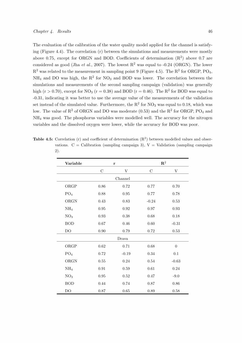
Chapter 4. Results 46
The evaluation of the calibration of the water quality model applied for the channel is satisfy-
ing (Figure 4.4). The correlation (r) between the simulations and measurements were mostly
above 0.75, except for ORGN and BOD. Coefficients of determination (R2) above 0.7 are
considered as good (Jha et al., 2007). The lowest R2 was equal to -0.24 (ORGN). The lower
R2 was related to the measurement in sampling point 9 (Figure 4.5). The R2 for ORGP, PO4,
NH4 and DO was high, the R2 for NO3 and BOD was lower. The correlation between the
simulations and measurements of the second sampling campaign (validation) was generally
high (r > 0.70), except for NO3 (r = 0.38) and BOD (r = 0.46). The R2 for BOD was equal to
-0.31, indicating it was better to use the average value of the measurements of the validation
set instead of the simulated value. Furthermore, the R2 for NO3 was equal to 0.18, which was
low. The value of R2 of ORGN and DO was moderate (0.53) and the R2 for ORGP, PO4 and
NH4 was good. The phosphorus variables were modelled well. The accuracy for the nitrogen
variables and the dissolved oxygen were lower, while the accuracy for BOD was poor.
Table 4.5: Correlation (r) and coefficient of determination (R2) between modelled values and obser-
vations. C = Calibration (sampling campaign 3), V = Validation (sampling campaign
2).
Variable r R2
C V C V
Channel
ORGP 0.86 0.72 0.77 0.70
PO4 0.88 0.95 0.77 0.78
ORGN 0.43 0.83 -0.24 0.53
NH4 0.95 0.92 0.97 0.93
NO3 0.93 0.38 0.68 0.18
BOD 0.67 0.46 0.60 -0.31
DO 0.90 0.79 0.72 0.53
Drava
ORGP 0.62 0.71 0.68 0
PO4 0.72 -0.19 0.34 0.1
ORGN 0.55 0.24 0.54 -0.63
NH4 0.91 0.59 0.61 0.24
NO3 0.95 0.52 0.47 -9.0
BOD 0.44 0.74 0.87 0.86
DO 0.87 0.65 0.89 0.58
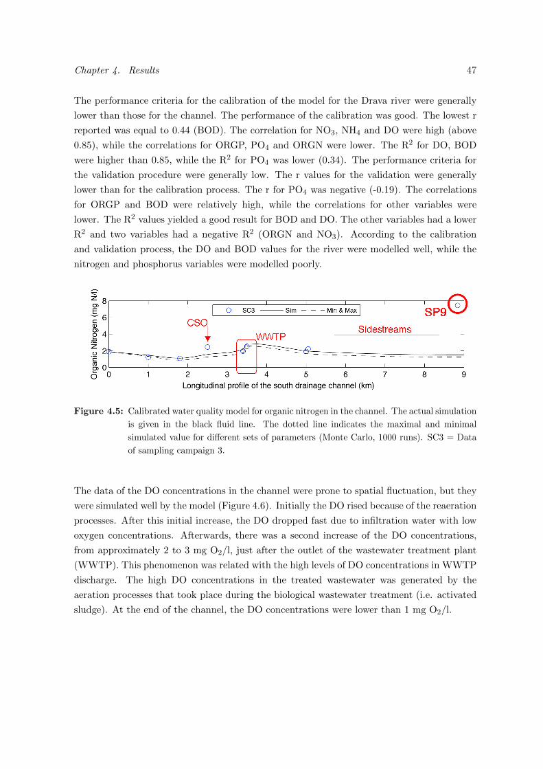
Chapter 4. Results 47
The performance criteria for the calibration of the model for the Drava river were generally
lower than those for the channel. The performance of the calibration was good. The lowest r
reported was equal to 0.44 (BOD). The correlation for NO3, NH4 and DO were high (above
0.85), while the correlations for ORGP, PO4 and ORGN were lower. The R2 for DO, BOD
were higher than 0.85, while the R2 for PO4 was lower (0.34). The performance criteria for
the validation procedure were generally low. The r values for the validation were generally
lower than for the calibration process. The r for PO4 was negative (-0.19). The correlations
for ORGP and BOD were relatively high, while the correlations for other variables were
lower. The R2 values yielded a good result for BOD and DO. The other variables had a lower
R2 and two variables had a negative R2 (ORGN and NO3). According to the calibration
and validation process, the DO and BOD values for the river were modelled well, while the
nitrogen and phosphorus variables were modelled poorly.
Figure 4.5: Calibrated water quality model for organic nitrogen in the channel. The actual simulation
is given in the black fluid line. The dotted line indicates the maximal and minimal
simulated value for different sets of parameters (Monte Carlo, 1000 runs). SC3 = Data
of sampling campaign 3.
The data of the DO concentrations in the channel were prone to spatial fluctuation, but they
were simulated well by the model (Figure 4.6). Initially the DO rised because of the reaeration
processes. After this initial increase, the DO dropped fast due to infiltration water with low
oxygen concentrations. Afterwards, there was a second increase of the DO concentrations,
from approximately 2 to 3 mg O2/l, just after the outlet of the wastewater treatment plant
(WWTP). This phenomenon was related with the high levels of DO concentrations in WWTP
discharge. The high DO concentrations in the treated wastewater was generated by the
aeration processes that took place during the biological wastewater treatment (i.e. activated
sludge). At the end of the channel, the DO concentrations were lower than 1 mg O2/l.
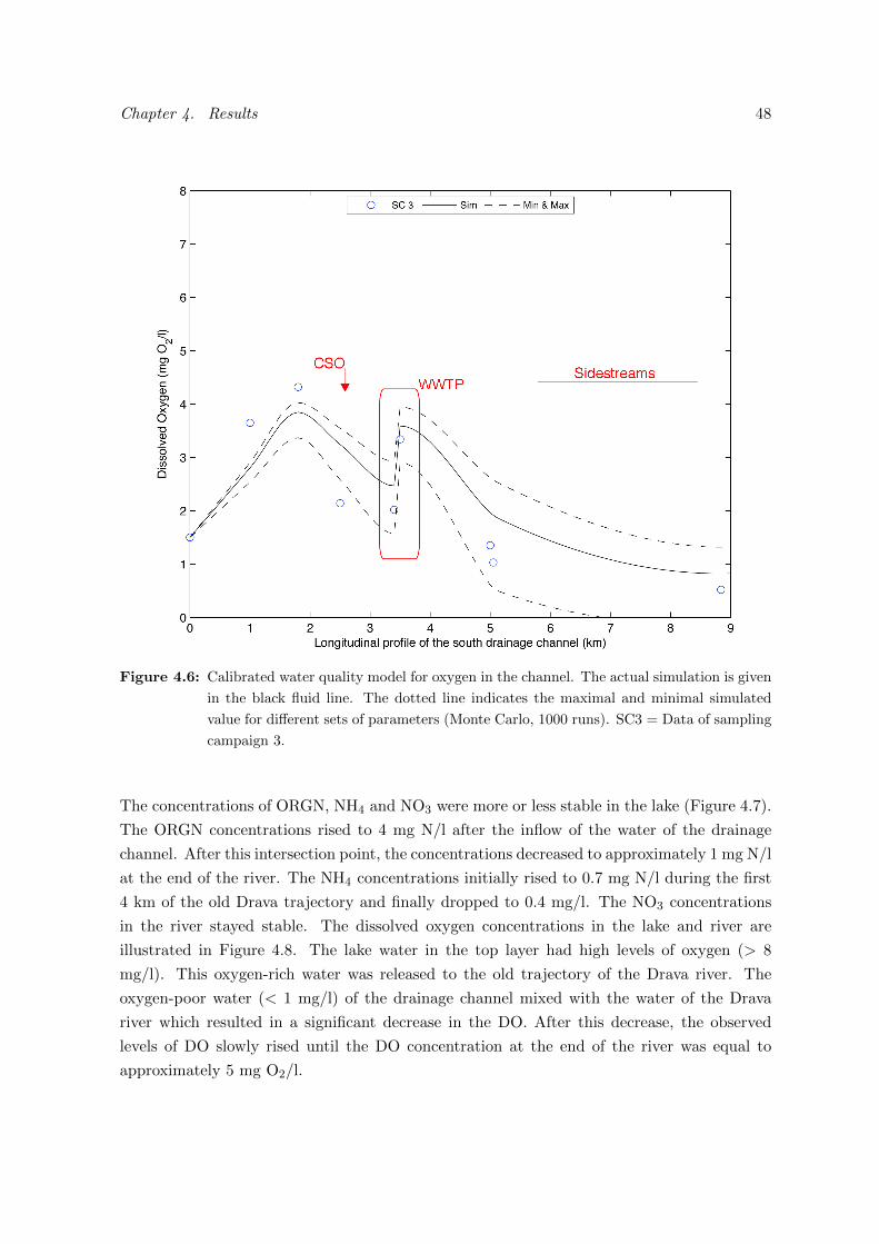
Chapter 4. Results 48
Figure 4.6: Calibrated water quality model for oxygen in the channel. The actual simulation is given
in the black fluid line. The dotted line indicates the maximal and minimal simulated
value for different sets of parameters (Monte Carlo, 1000 runs). SC3 = Data of sampling
campaign 3.
The concentrations of ORGN, NH4 and NO3 were more or less stable in the lake (Figure 4.7).
The ORGN concentrations rised to 4 mg N/l after the inflow of the water of the drainage
channel. After this intersection point, the concentrations decreased to approximately 1 mg N/l
at the end of the river. The NH4 concentrations initially rised to 0.7 mg N/l during the first
4 km of the old Drava trajectory and finally dropped to 0.4 mg/l. The NO3 concentrations
in the river stayed stable. The dissolved oxygen concentrations in the lake and river are
illustrated in Figure 4.8. The lake water in the top layer had high levels of oxygen (> 8
mg/l). This oxygen-rich water was released to the old trajectory of the Drava river. The
oxygen-poor water (< 1 mg/l) of the drainage channel mixed with the water of the Drava
river which resulted in a significant decrease in the DO. After this decrease, the observed
levels of DO slowly rised until the DO concentration at the end of the river was equal to
approximately 5 mg O2/l.
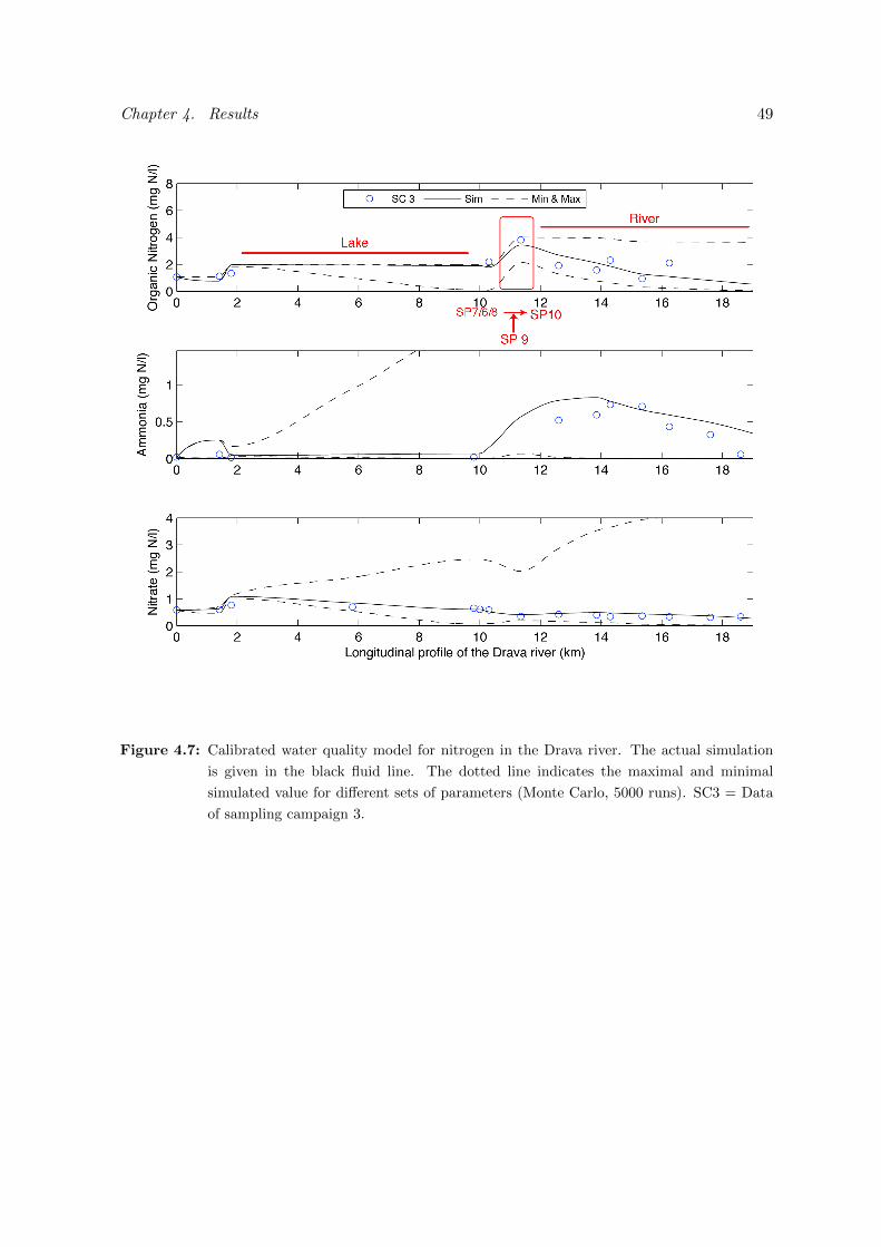
Chapter 4. Results 49
Figure 4.7: Calibrated water quality model for nitrogen in the Drava river. The actual simulation
is given in the black fluid line. The dotted line indicates the maximal and minimal
simulated value for different sets of parameters (Monte Carlo, 5000 runs). SC3 = Data
of sampling campaign 3.
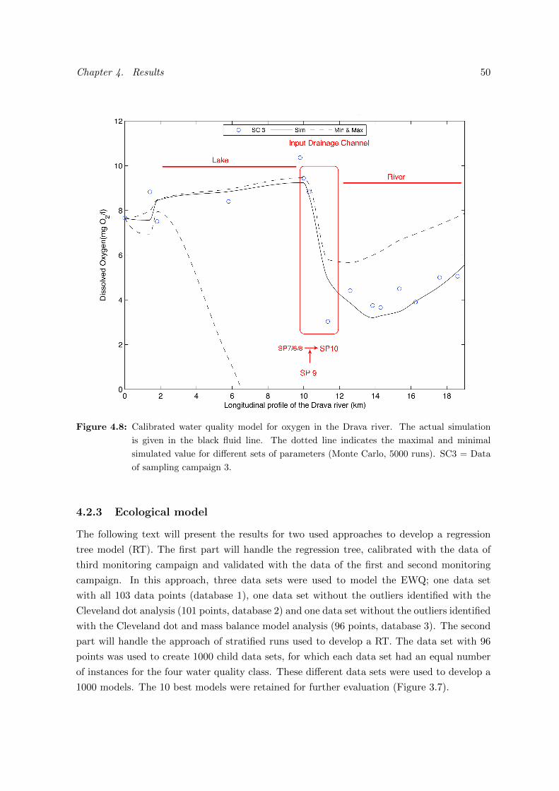
Chapter 4. Results 50
Figure 4.8: Calibrated water quality model for oxygen in the Drava river. The actual simulation
is given in the black fluid line. The dotted line indicates the maximal and minimal
simulated value for different sets of parameters (Monte Carlo, 5000 runs). SC3 = Data
of sampling campaign 3.
4.2.3 Ecological model
The following text will present the results for two used approaches to develop a regression
tree model (RT). The first part will handle the regression tree, calibrated with the data of
third monitoring campaign and validated with the data of the first and second monitoring
campaign. In this approach, three data sets were used to model the EWQ; one data set
with all 103 data points (database 1), one data set without the outliers identified with the
Cleveland dot analysis (101 points, database 2) and one data set without the outliers identified
with the Cleveland dot and mass balance model analysis (96 points, database 3). The second
part will handle the approach of stratified runs used to develop a RT. The data set with 96
points was used to create 1000 child data sets, for which each data set had an equal number
of instances for the four water quality class. These different data sets were used to develop a
1000 models. The 10 best models were retained for further evaluation (Figure 3.7).
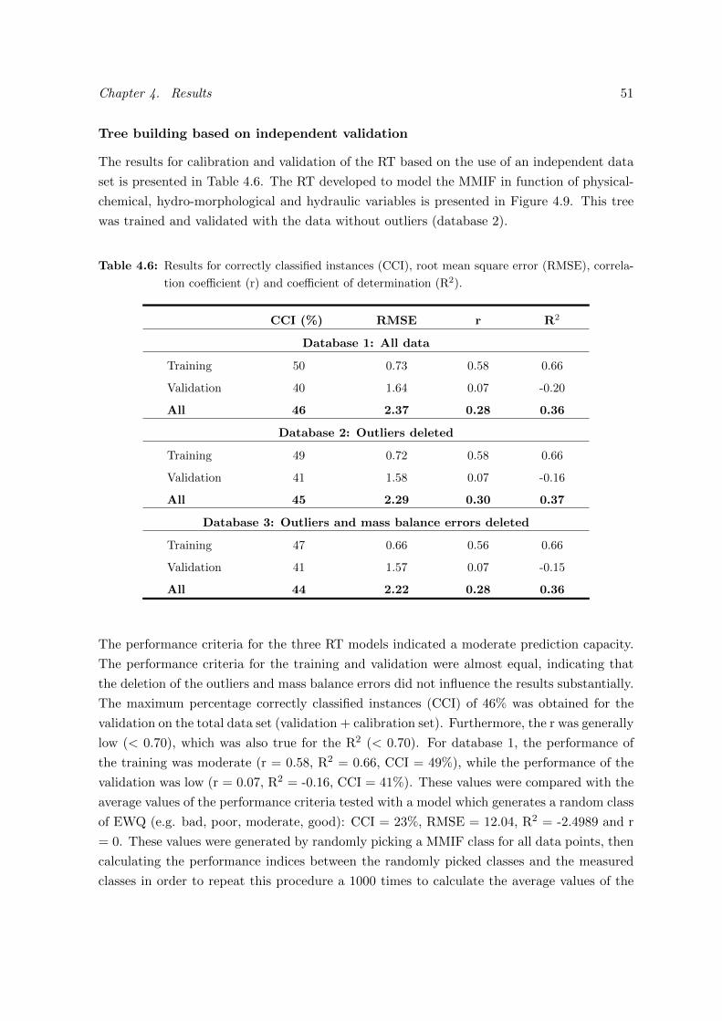
Chapter 4. Results 51
Tree building based on independent validation
The results for calibration and validation of the RT based on the use of an independent data
set is presented in Table 4.6. The RT developed to model the MMIF in function of physical-
chemical, hydro-morphological and hydraulic variables is presented in Figure 4.9. This tree
was trained and validated with the data without outliers (database 2).
Table 4.6: Results for correctly classified instances (CCI), root mean square error (RMSE), correla-
tion coefficient (r) and coefficient of determination (R2).
CCI (%) RMSE r R2
Database 1: All data
Training 50 0.73 0.58 0.66
Validation 40 1.64 0.07 -0.20
All 46 2.37 0.28 0.36
Database 2: Outliers deleted
Training 49 0.72 0.58 0.66
Validation 41 1.58 0.07 -0.16
All 45 2.29 0.30 0.37
Database 3: Outliers and mass balance errors deleted
Training 47 0.66 0.56 0.66
Validation 41 1.57 0.07 -0.15
All 44 2.22 0.28 0.36
The performance criteria for the three RT models indicated a moderate prediction capacity.
The performance criteria for the training and validation were almost equal, indicating that
the deletion of the outliers and mass balance errors did not influence the results substantially.
The maximum percentage correctly classified instances (CCI) of 46% was obtained for the
validation on the total data set (validation + calibration set). Furthermore, the r was generally
low (< 0.70), which was also true for the R2 (< 0.70). For database 1, the performance of
the training was moderate (r = 0.58, R2 = 0.66, CCI = 49%), while the performance of the
validation was low (r = 0.07, R2 = -0.16, CCI = 41%). These values were compared with the
average values of the performance criteria tested with a model which generates a random class
of EWQ (e.g. bad, poor, moderate, good): CCI = 23%, RMSE = 12.04, R2 = -2.4989 and r
= 0. These values were generated by randomly picking a MMIF class for all data points, then
calculating the performance indices between the randomly picked classes and the measured
classes in order to repeat this procedure a 1000 times to calculate the average values of the
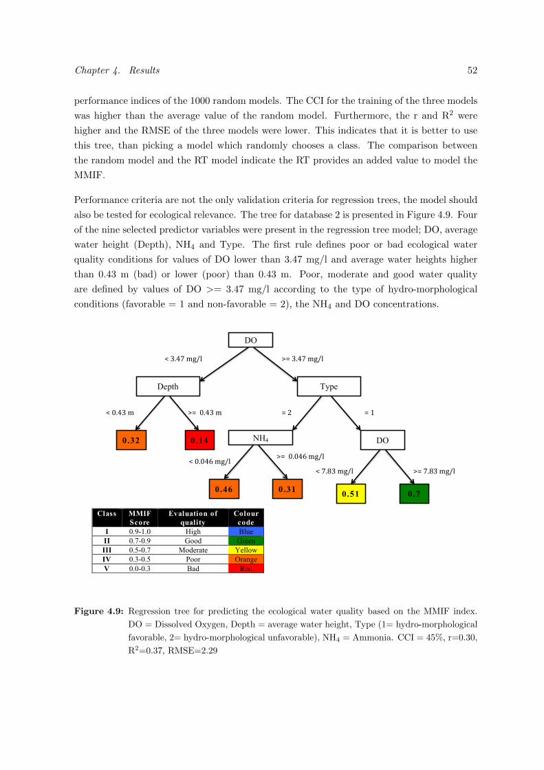
Chapter 4. Results 52
performance indices of the 1000 random models. The CCI for the training of the three models
was higher than the average value of the random model. Furthermore, the r and R2 were
higher and the RMSE of the three models were lower. This indicates that it is better to use
this tree, than picking a model which randomly chooses a class. The comparison between
the random model and the RT model indicate the RT provides an added value to model the
MMIF.
Performance criteria are not the only validation criteria for regression trees, the model should
also be tested for ecological relevance. The tree for database 2 is presented in Figure 4.9. Four
of the nine selected predictor variables were present in the regression tree model; DO, average
water height (Depth), NH4 and Type. The first rule defines poor or bad ecological water
quality conditions for values of DO lower than 3.47 mg/l and average water heights higher
than 0.43 m (bad) or lower (poor) than 0.43 m. Poor, moderate and good water quality
are defined by values of DO >= 3.47 mg/l according to the type of hydro-morphological
conditions (favorable = 1 and non-favorable = 2), the NH4 and DO concentrations.
!"##$%&'#(#
0.14
0.46
Depth
0.31
NH4
44 !"##$%$&)#(*+,#
0.51 0.7
#
#
#
#
#
#
#
#
#
#
#
#
#
#
#
#
#
#
#
#
#
#
#
#
#
Class MMIF
Score
Evaluation of
quality
Colour
code
I 0.9-1.0 High Blue
II 0.7-0.9 Good Green
III 0.5-0.7 Moderate Yellow
IV 0.3-0.5 Poor Orange
V 0.0-0.3 Bad Red
DO
Type
DO
-#'%&.#(*+,# !"#'%&.#(*+,#
"#/#-#$%&'#(#
-#.%0'#(*+,##
0.32
-#$%$&)#(*+,#
"#1#
!"#.%0'#(*+,#
Figure 4.9: Regression tree for predicting the ecological water quality based on the MMIF index.
DO = Dissolved Oxygen, Depth = average water height, Type (1= hydro-morphological
favorable, 2= hydro-morphological unfavorable), NH4 = Ammonia. CCI = 45%, r=0.30,
R2=0.37, RMSE=2.29
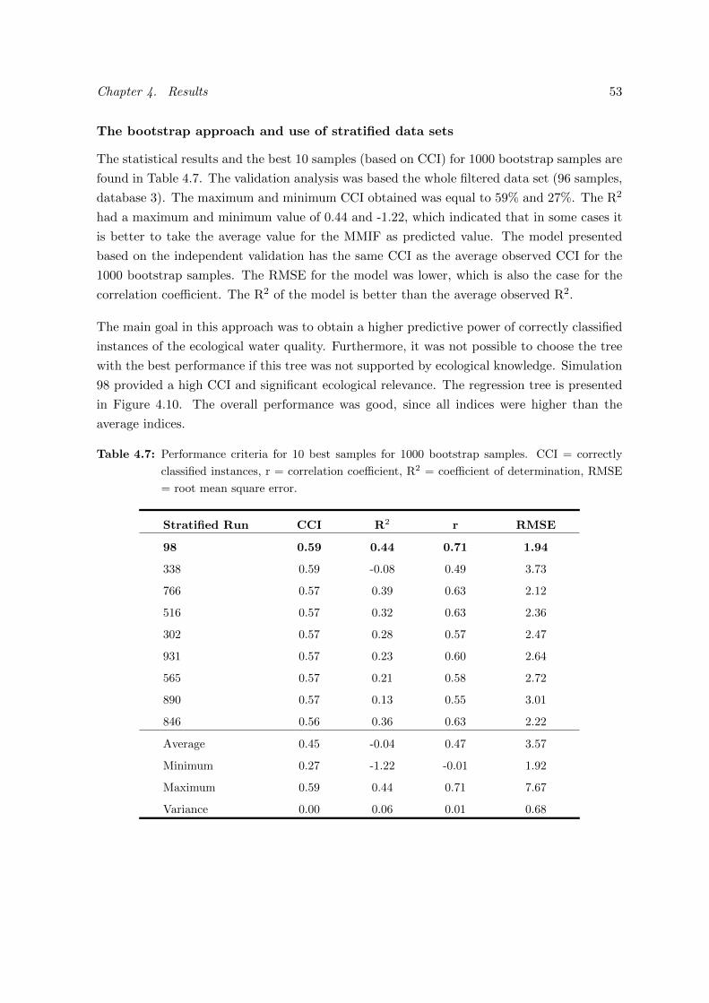
Chapter 4. Results 53
The bootstrap approach and use of stratified data sets
The statistical results and the best 10 samples (based on CCI) for 1000 bootstrap samples are
found in Table 4.7. The validation analysis was based the whole filtered data set (96 samples,
database 3). The maximum and minimum CCI obtained was equal to 59% and 27%. The R2
had a maximum and minimum value of 0.44 and -1.22, which indicated that in some cases it
is better to take the average value for the MMIF as predicted value. The model presented
based on the independent validation has the same CCI as the average observed CCI for the
1000 bootstrap samples. The RMSE for the model was lower, which is also the case for the
correlation coefficient. The R2 of the model is better than the average observed R2.
The main goal in this approach was to obtain a higher predictive power of correctly classified
instances of the ecological water quality. Furthermore, it was not possible to choose the tree
with the best performance if this tree was not supported by ecological knowledge. Simulation
98 provided a high CCI and significant ecological relevance. The regression tree is presented
in Figure 4.10. The overall performance was good, since all indices were higher than the
average indices.
Table 4.7: Performance criteria for 10 best samples for 1000 bootstrap samples. CCI = correctly
classified instances, r = correlation coefficient, R2 = coefficient of determination, RMSE
= root mean square error.
Stratified Run CCI R2 r RMSE
98 0.59 0.44 0.71 1.94
338 0.59 -0.08 0.49 3.73
766 0.57 0.39 0.63 2.12
516 0.57 0.32 0.63 2.36
302 0.57 0.28 0.57 2.47
931 0.57 0.23 0.60 2.64
565 0.57 0.21 0.58 2.72
890 0.57 0.13 0.55 3.01
846 0.56 0.36 0.63 2.22
Average 0.45 -0.04 0.47 3.57
Minimum 0.27 -1.22 -0.01 1.92
Maximum 0.59 0.44 0.71 7.67
Variance 0.00 0.06 0.01 0.68
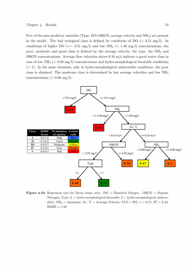
Chapter 4. Results 54
Five of the nine predictor variables (Type, DO, ORGN, average velocity and NH4) are present
in the model. The bad ecological class is defined by conditions of DO (< 3.51 mg/l). In
conditions of higher DO (>= 3.51 mg/l) and low NH4 (< 1.48 mg/l) concentrations, the
poor, moderate and good class is defined by the average velocity, the type, the NH4 and
ORGN concentrations. Average flow velocities above 0.16 m/s indicate a good water class in
case of low NH4 (< 0.08 mg/l) concentrations and hydro-morphological favorable conditions
(= 1). In the same situation, only in hydro-morphological unfavorable conditions, the poor
class is obtained. The moderate class is determined by low average velocities and low NH4
concentrations (< 0.08 mg/l).
0.05 Av. V
44
0.28 0.47
NH4
44
ORGN
44
Type
0.15
0.38
0.73 0.48
0.4 0.67
!
!
!
!
!
!
!
!
!
!
!
!
!
!
!
!
!
!
!
!
!
! !
Class MMIF
Score
Evaluation
of quality
Colour
code
I 0.9-1.0 High Blue
II 0.7-0.9 Good Green
III 0.5-0.7 Moderate Yellow
IV 0.3-0.5 Poor Orange
V 0.0-0.3 Bad Red
DO
NH4
"!#$%&!'()*!
"!&$+,!'()*!-.!&$+,!'()*!
-.!#$%&!'()*!
-.!/$&0!')1!"!/$&0!')1!
-.!/$/,!'()*!"!/$/,!'()*!
.!&!.!2!
-.!2$3%!'()*!"!!2$3%!'()*!
Figure 4.10: Regression tree for Drava study area. DO = Dissolved Oxygen , ORGN = Organic
Nitrogen, Type (1 = hydro-morphological favorable, 2 = hydro-morphological unfavor-
able), NH4 = Ammonia, Av. V = Average Velocity. CCI = 59%, r = 0.71, R2 = 0.44,
RMSE = 1.94
Chapter 5
Discussion
5.1 Model development
5.1.1 Data collection and analysis
The framework, which was presented in this thesis (Figure 3.3 in the methodology) required in-
formation and data in several domains (e.g. hydraulics, physical-chemical parameters, hydro-
morphology, ecological). Furthermore, the data needed a good and accurate analysis, in order
to identify possible outliers. It was required to keep as much as possible valuable information
for the water quality and regression tree models (RT).
The outlier analysis was performed with three methods: box plots, Cleveland dot plots and
mass balances. The first method, the box plots, yielded the loss of 15 data points, while
the second method, the Cleveland dot plots, yielded the loss of two points. As depicted
by Zuur et al. (2010), box plots are not always the best solution to delete outliers. For
example, concentrations of ammonia in the river can be very high close to the discharge point
of a wastewater treatment facility. The use of box plots to delete the outliers could identify
the high ammonia concentration as an outlier. Removal of this point can be identified as
a “wrongly” removed data point. In the framework of water quality modelling it might be
better not to delete the data point, because it can hold valuable information of the relation
between the physical-chemical status and the biological status. Cleveland dot plots can offer
the solution, but compared to box plots, the analysis is more subjective. The third method,
the mass balance method, yielded the loss of five points. Also this method is more subjective,
because there are no quantifying criteria used to delete these data points. In this framework,
the combination of the Cleveland dot plots and the mass balance model was used. In order
to use this approach, the author stresses that the modeller must have significant knowledge
about the details of the system and sampling conditions (how, where and when were they
taken).
55
Chapter 5. Discussion 56
As indicated by Vayssieres et al. (2000), RT are robust against outlier data. In this research
at the Drava river, this property was illustrated. Three RT were developed for predicting the
Multimetric Macroinvertebrate Index of Flanders (MMIF) and the ecological water quality
(EWQ) class based on three data set; one with all data (103 points), one without outliers
identified with the Cleveland dot plots (101 points) and one without outliers identified with
Cleveland dot plots and the mass balance model (96 points). The performance indices, the
tree structure and the rules of all three models were almost identical. If certain outliers in
data sets are not directly explained by a possible condition or impact, the removal of the data
point is subject for debate. If RT are used to model the MMIF, these data points can be
retained in the data set without changing the results considerably.
5.1.2 Model calibration and validation
All the physical-chemical variables of the channel were modelled well, expect for the variable
biological oxygen demand (BOD) which had low performance for the validation. The BOD
and dissolved oxygen (DO) of the Drava river were modelled accurate, while the nitrogen and
phosphorus variables were modelled less well. Especially for the validation, the nitrogen and
phosphorus concentrations were simulated poorly. This might be related to the lower amount
of data which was available for the validation.
The values of the calibrated parameters were fairly in the range of the expected values. The
process rates in the lake were generally lower, indicating a slower turn-over rate. As indicated
by Shanahan et al. (1998), the determination of the reaeration coefficient is generally prob-
lematic in small rivers (e.g. channel). The implemented formulas did not yield the expected
results and that is why the reaeration rates were calibrated in function of the waterbody and
stretch properties (Table 3.3). The determination of the constant value results in a value
which might not be transferable to other conditions. The reaeration coefficient in rivers is
typically a function of the temperature and simple hydraulic characteristics such as stream
depth and velocity (Bowie et al., 1985). The reaeration processes in the lakes are mainly
driven by wind effects (Bowie et al., 1985) and since the considered lakes is located in a open
environment, the wind effects will significantly influence the oxygen balance in the lake. Sedi-
mentation and settling processes of suspended solids and solutes are very important processes
in lakes. The calibrated parameters (settling velocity of organic matter and phosphorus) for
the lake did not support this theory, but they do support the statement of Bonacci & Oskorus
(2008), which states that there is no significant sedimentation (and settling) in the Croatian
reservoirs (Varazdin, Cakovec and Dubrava) during their existence.
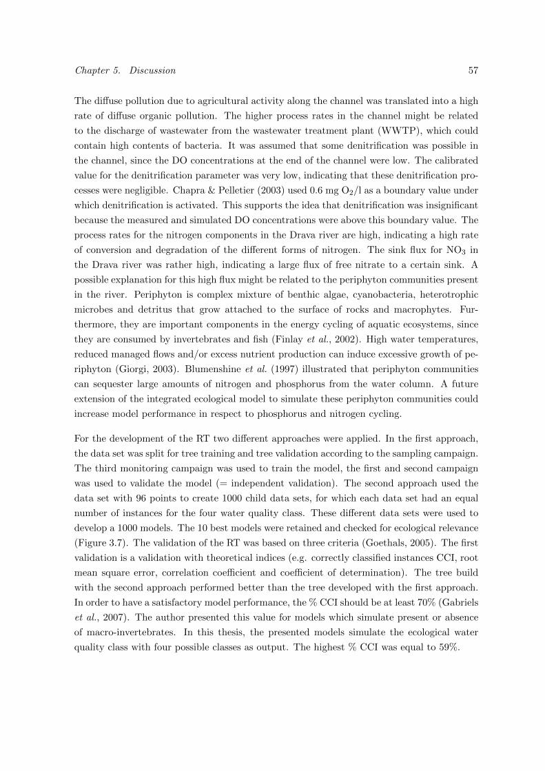
Chapter 5. Discussion 57
The diffuse pollution due to agricultural activity along the channel was translated into a high
rate of diffuse organic pollution. The higher process rates in the channel might be related
to the discharge of wastewater from the wastewater treatment plant (WWTP), which could
contain high contents of bacteria. It was assumed that some denitrification was possible in
the channel, since the DO concentrations at the end of the channel were low. The calibrated
value for the denitrification parameter was very low, indicating that these denitrification pro-
cesses were negligible. Chapra & Pelletier (2003) used 0.6 mg O2/l as a boundary value under
which denitrification is activated. This supports the idea that denitrification was insignificant
because the measured and simulated DO concentrations were above this boundary value. The
process rates for the nitrogen components in the Drava river are high, indicating a high rate
of conversion and degradation of the different forms of nitrogen. The sink flux for NO3 in
the Drava river was rather high, indicating a large flux of free nitrate to a certain sink. A
possible explanation for this high flux might be related to the periphyton communities present
in the river. Periphyton is complex mixture of benthic algae, cyanobacteria, heterotrophic
microbes and detritus that grow attached to the surface of rocks and macrophytes. Fur-
thermore, they are important components in the energy cycling of aquatic ecosystems, since
they are consumed by invertebrates and fish (Finlay et al., 2002). High water temperatures,
reduced managed flows and/or excess nutrient production can induce excessive growth of pe-
riphyton (Giorgi, 2003). Blumenshine et al. (1997) illustrated that periphyton communities
can sequester large amounts of nitrogen and phosphorus from the water column. A future
extension of the integrated ecological model to simulate these periphyton communities could
increase model performance in respect to phosphorus and nitrogen cycling.
For the development of the RT two different approaches were applied. In the first approach,
the data set was split for tree training and tree validation according to the sampling campaign.
The third monitoring campaign was used to train the model, the first and second campaign
was used to validate the model (= independent validation). The second approach used the
data set with 96 points to create 1000 child data sets, for which each data set had an equal
number of instances for the four water quality class. These different data sets were used to
develop a 1000 models. The 10 best models were retained and checked for ecological relevance
(Figure 3.7). The validation of the RT was based on three criteria (Goethals, 2005). The first
validation is a validation with theoretical indices (e.g. correctly classified instances CCI, root
mean square error, correlation coefficient and coefficient of determination). The tree build
with the second approach performed better than the tree developed with the first approach.
In order to have a satisfactory model performance, the % CCI should be at least 70% (Gabriels
et al., 2007). The author presented this value for models which simulate present or absence
of macro-invertebrates. In this thesis, the presented models simulate the ecological water
quality class with four possible classes as output. The highest % CCI was equal to 59%.
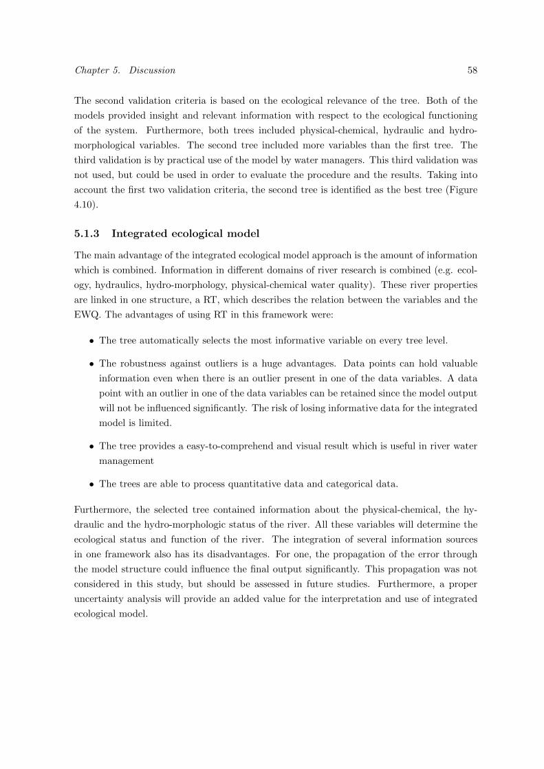
Chapter 5. Discussion 58
The second validation criteria is based on the ecological relevance of the tree. Both of the
models provided insight and relevant information with respect to the ecological functioning
of the system. Furthermore, both trees included physical-chemical, hydraulic and hydro-
morphological variables. The second tree included more variables than the first tree. The
third validation is by practical use of the model by water managers. This third validation was
not used, but could be used in order to evaluate the procedure and the results. Taking into
account the first two validation criteria, the second tree is identified as the best tree (Figure
4.10).
5.1.3 Integrated ecological model
The main advantage of the integrated ecological model approach is the amount of information
which is combined. Information in different domains of river research is combined (e.g. ecol-
ogy, hydraulics, hydro-morphology, physical-chemical water quality). These river properties
are linked in one structure, a RT, which describes the relation between the variables and the
EWQ. The advantages of using RT in this framework were:
• The tree automatically selects the most informative variable on every tree level.
• The robustness against outliers is a huge advantages. Data points can hold valuable
information even when there is an outlier present in one of the data variables. A data
point with an outlier in one of the data variables can be retained since the model output
will not be influenced significantly. The risk of losing informative data for the integrated
model is limited.
• The tree provides a easy-to-comprehend and visual result which is useful in river water
management
• The trees are able to process quantitative data and categorical data.
Furthermore, the selected tree contained information about the physical-chemical, the hy-
draulic and the hydro-morphologic status of the river. All these variables will determine the
ecological status and function of the river. The integration of several information sources
in one framework also has its disadvantages. For one, the propagation of the error through
the model structure could influence the final output significantly. This propagation was not
considered in this study, but should be assessed in future studies. Furthermore, a proper
uncertainty analysis will provide an added value for the interpretation and use of integrated
ecological model.
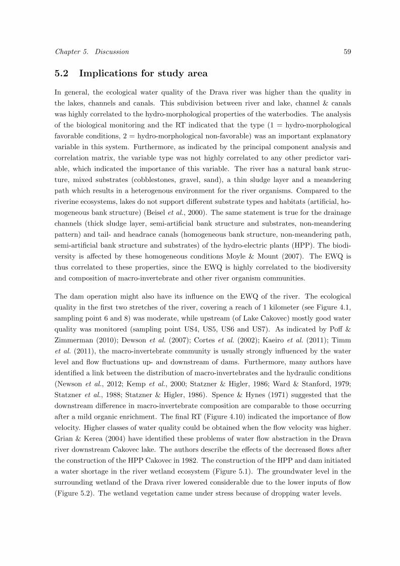
Chapter 5. Discussion 59
5.2 Implications for study area
In general, the ecological water quality of the Drava river was higher than the quality in
the lakes, channels and canals. This subdivision between river and lake, channel & canals
was highly correlated to the hydro-morphological properties of the waterbodies. The analysis
of the biological monitoring and the RT indicated that the type (1 = hydro-morphological
favorable conditions, 2 = hydro-morphological non-favorable) was an important explanatory
variable in this system. Furthermore, as indicated by the principal component analysis and
correlation matrix, the variable type was not highly correlated to any other predictor vari-
able, which indicated the importance of this variable. The river has a natural bank struc-
ture, mixed substrates (cobblestones, gravel, sand), a thin sludge layer and a meandering
path which results in a heterogenous environment for the river organisms. Compared to the
riverine ecosystems, lakes do not support different substrate types and habitats (artificial, ho-
mogeneous bank structure) (Beisel et al., 2000). The same statement is true for the drainage
channels (thick sludge layer, semi-artificial bank structure and substrates, non-meandering
pattern) and tail- and headrace canals (homogeneous bank structure, non-meandering path,
semi-artificial bank structure and substrates) of the hydro-electric plants (HPP). The biodi-
versity is affected by these homogeneous conditions Moyle & Mount (2007). The EWQ is
thus correlated to these properties, since the EWQ is highly correlated to the biodiversity
and composition of macro-invertebrate and other river organism communities.
The dam operation might also have its influence on the EWQ of the river. The ecological
quality in the first two stretches of the river, covering a reach of 1 kilometer (see Figure 4.1,
sampling point 6 and 8) was moderate, while upstream (of Lake Cakovec) mostly good water
quality was monitored (sampling point US4, US5, US6 and US7). As indicated by Poff &
Zimmerman (2010); Dewson et al. (2007); Cortes et al. (2002); Kaeiro et al. (2011); Timm
et al. (2011), the macro-invertebrate community is usually strongly influenced by the water
level and flow fluctuations up- and downstream of dams. Furthermore, many authors have
identified a link between the distribution of macro-invertebrates and the hydraulic conditions
(Newson et al., 2012; Kemp et al., 2000; Statzner & Higler, 1986; Ward & Stanford, 1979;
Statzner et al., 1988; Statzner & Higler, 1986). Spence & Hynes (1971) suggested that the
downstream difference in macro-invertebrate composition are comparable to those occurring
after a mild organic enrichment. The final RT (Figure 4.10) indicated the importance of flow
velocity. Higher classes of water quality could be obtained when the flow velocity was higher.
Grian & Kerea (2004) have identified these problems of water flow abstraction in the Drava
river downstream Cakovec lake. The authors describe the effects of the decreased flows after
the construction of the HPP Cakovec in 1982. The construction of the HPP and dam initiated
a water shortage in the river wetland ecosystem (Figure 5.1). The groundwater level in the
surrounding wetland of the Drava river lowered considerable due to the lower inputs of flow
(Figure 5.2). The wetland vegetation came under stress because of dropping water levels.
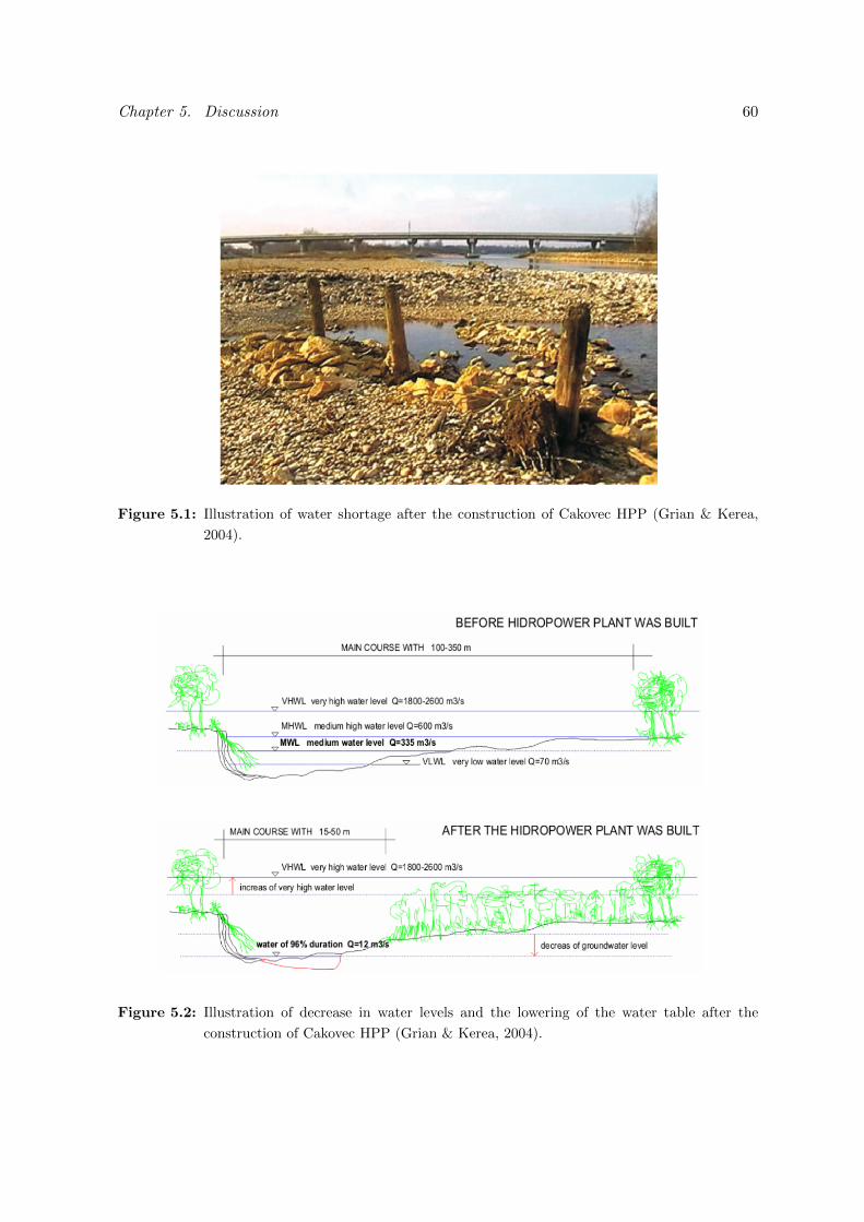
Chapter 5. Discussion 60
Figure 5.1: Illustration of water shortage after the construction of Cakovec HPP (Grian & Kerea,
2004).
Figure 5.2: Illustration of decrease in water levels and the lowering of the water table after the
construction of Cakovec HPP (Grian & Kerea, 2004).
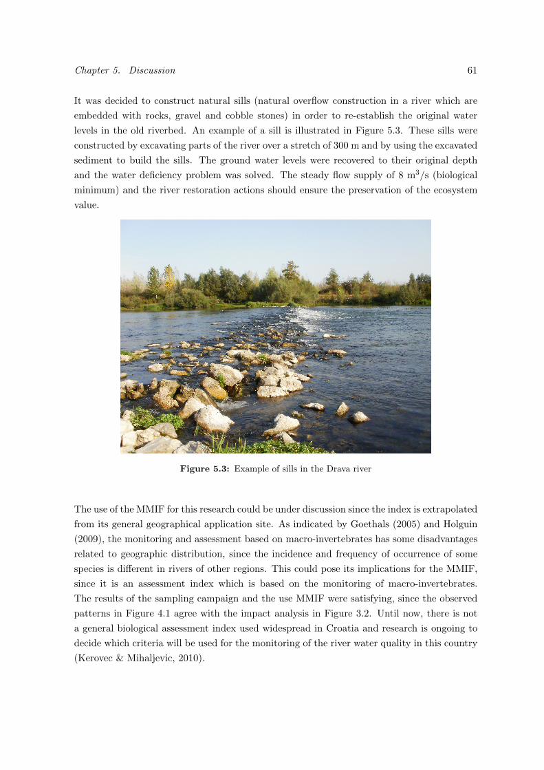
Chapter 5. Discussion 61
It was decided to construct natural sills (natural overflow construction in a river which are
embedded with rocks, gravel and cobble stones) in order to re-establish the original water
levels in the old riverbed. An example of a sill is illustrated in Figure 5.3. These sills were
constructed by excavating parts of the river over a stretch of 300 m and by using the excavated
sediment to build the sills. The ground water levels were recovered to their original depth
and the water deficiency problem was solved. The steady flow supply of 8 m3/s (biological
minimum) and the river restoration actions should ensure the preservation of the ecosystem
value.
Figure 5.3: Example of sills in the Drava river
The use of the MMIF for this research could be under discussion since the index is extrapolated
from its general geographical application site. As indicated by Goethals (2005) and Holguin
(2009), the monitoring and assessment based on macro-invertebrates has some disadvantages
related to geographic distribution, since the incidence and frequency of occurrence of some
species is different in rivers of other regions. This could pose its implications for the MMIF,
since it is an assessment index which is based on the monitoring of macro-invertebrates.
The results of the sampling campaign and the use MMIF were satisfying, since the observed
patterns in Figure 4.1 agree with the impact analysis in Figure 3.2. Until now, there is not
a general biological assessment index used widespread in Croatia and research is ongoing to
decide which criteria will be used for the monitoring of the river water quality in this country
(Kerovec & Mihaljevic, 2010).
Chapter 5. Discussion 62
The impact of the physical-chemical status on the biological water quality of the river system
is the last important element in the system analysis. The biological assessment map (Figure
4.1) in the results indicated an impact of the drainage channel on the biological functioning of
the Drava river ecosystem. Furthermore, the water quality in the southern drainage channel,
which receives the wastewater discharge, was in average a water quality class lower than in
the northern drainage channel. The analysis of the simulations of the water quality model
indicated a fair dilution of the treated and untreated wastewater with oxygen-poor infiltration
water. Mainly the concentrations of organic nitrogen and ammonia showed an increase in the
Drava river after the joint with the southern drainage channel. The importance of organic
nitrogen and ammonia were also illustrated in the selected tree, where higher concentrations
resulted in lower water quality. Furthermore, the infiltration water with low DO coming
from the lake resulted in low and moderate oxygen levels in respectively the channel and
the river. The higher pollution load in the southern drainage channel was linked to the
discharge of treated and untreated wastewater in the channel. The side streams which mouth
in the channel seemed to have a limited influence on the physical-chemical water quality. The
WWTP had a significant influence. The stakeholders and WWTP managers are aware of the
influence and, as depicted by Kezelj et al. (2010), the pressure on the municipal WWTP is
rising mainly by an increased input of industrial wastewater.
Chapter 6
Conclusions and future perspectives
This study has illustrated the high potential of integrated ecological models. The framework
for the integrated ecological model was able to integrate all water quality driving variables
(physical-chemical, hydraulic, hydro-morphological and biological variables) in one structure
in order to quantify the major impacts. This approach contributes significantly to the insight
and knowledge of the ecological functioning of river ecosystems. The integrated model is a
powerful and effictive tool, because it is able to asses the ecological impacts of wastewater
discharges and dam operations on the Drava river. This research creates opportunities and
perspectives for the involved parties and stakeholders to reconsider elements in the water
management of the system. As indicated in the introduction, the Drava river in Croatia is
a river ecosystem with an unique value. It is up to the involved instances to preserve this
valuable ecosystem.
The key elements in the integrated ecological model were the water quality and regression
tree model. The performance of the calibration of the water quality model was good, while
the performance for the validation was lower. Possible future extentensions of the model
structure should be focus on modelling of algae and bacteria in order to yield better results.
An interesting approach which could be used for the water quality model could be the one
adopted by Reichert et al. (2001) for the development in the river water quality model no. 1
(RWQM no1). The goal of this model was to integrate a sewer, wastewater treatment and
river water quality model in one integrated framework. An advantages of the model is that it
is based on chemical oxygen demand (COD) modelling which makes it possible to close the
mass balance for carbon. Furthermore, the RWQM no1 is able to simulate microbial biomass
in the river column (Shanahan et al., 1998; Somlyody et al., 1998).
63
Chapter 6. Conclusions and future perspectives 64
The regression tree developed for the ecological assessment model provided an added value
to model the ecological water class. The bootstrap approach proved to be useful to find a
tree with satisfying performance criteria and relevant ecological information. As indicated
by Gabriels et al. (2007), the % CCI should at least be 70% for simulating 2 classes. In this
research, a maximum % CCI of 59% was obtained for a model which simulates 4 classes. The
selected tree provided significant insight in the ecological functioning of the Drava river. The
use of regression trees in this framework was very useful. The tree automatically selected the
most informative variables. The robustness of the trees to outliers was a huge advantages.
Data points can hold valuable information even when there is a outlier present in one of the
data variables. A data point with an outlier in one of the data variables can be retained
since the model output will not be influenced significantly. Additionally, the tree provided an
easy-to-comprehend and visual result, which is useful in river water management.
Additional data should be collected in order to increase model performance. Future moni-
toring should focus on sampling locations in the old trajectory of the Drava river in order
to increase knowledge about the functioning of the river ecosystem. More samples should be
collected in the river upstream of Cakovec lake, since this serves as a reference condition for
the river downstream. Additionally, the technical global performance and the propagation of
the error in the integrated ecological model should be assessed in future studies. A proper
uncertainty analysis should be performed and the relevance in practice and applicability of
the model should be evaluated. When these elements are taken into account, the model will
be able to simulate different scenario’s. These scenario’s can support decission making in
river managment.
The dam construction and its operations might have a influence on the functioning of the
system. Water shortage in the system was an issue after the construction of the hydro-electric
plants and might, till this day, still be an issue. The current biological minimum flow of 8
m3/s (minimal flow which should be released to the Drava river) might not be sufficient
to preserve the natural value of the river. It is possible that the value of 8 m3/s should
be reconsidered. Future studies could asses whether this value is high enough to guarantee
the preservation of the Drava river. Furthermore, the impact of the discharge of treated
and untreated wastewater on this river should be closely followed in future studies. The
pressure on the wastewater treatment plant (WWTP) of the city of Varazdin is rising due
to increased industrial activity in the city of Varazdin. In perspective of growing pressures
and impacts, the efficiency and capacity of the WWTP plant could be reconsidered for future
optimizations. Furthermore, the discharge regulations for the industries in this study area
could be reconsidered in order to decrease pressure on the WWTP.
References
Ahmadi-Nedushan, B., St-Hilaire, A., Berube, M., Robichaud, E., Thiemonge, N. & Bobee,
B. (2006). A review of statistical methods for the evaluation of aquatic habitat suitability
for instream flow assessment. RIVER RESEARCH AND APPLICATIONS, 22(5):503–523.
ISSN 1535-1459.
Ambelu, A., Lock, K. & Goethals, P. (2010). Comparison of modelling techniques to predict
macroinvertebrate community composition in rivers of Ethiopia. ECOLOGICAL INFOR-
MATICS, 5(2):147–152. ISSN 1574-9541.
Apha (2005). Standard methods for the examination of water and wastewater, volume 2009.
American Public Health Association.
Barre de Saint-Venant, A. (1871). Theorie du Mouvement Non Permanent des Eaux, avec
Application aux Crues de Rivieres et ‘a l’Introduction des Marees dans leur Lit. Comptes
Rendus des seances de l’Academie des Sciences, Paris, France.
Beisel, J., Usseglio-Polatera, P. & Moreteau, J. (2000). The spatial heterogeneity of a river
bottom: a key factor determining macroinvertebrate communities. HYDROBIOLOGIA,
422:163–171. ISSN 0018-8158. International Conference on Assessing the Ecological In-
tegrity of Running Waters, UNIV AGR SCI, DEPT HYDROBIO, VIENNA, AUSTRIA,
NOV, 1998.
Benedetti, L., Meirlaen, J., Sforzi, F., Facchi, A., Gandolfi, C. & Vanrolleghem, P. A. (2007).
Dynamic integrated water quality modelling: A case study of the Lambro River, northern
Italy. WATER SA, 33(5):627–632. ISSN 0378-4738.
Benedetti, L. & Sforzi, F. (1999). Dynamic Integrated Modelling: A Case Study On The
Lambro Catchment. Ph.D. thesis, University of Ghent, UGent.
Blumenshine, S., Vadeboncoeur, Y., Lodge, D., Cottingham, K. & Knight, S. (1997). Benthic-
pelagic links: responses of benthos to water-column nutrient enrichment. JOURNAL OF
THE NORTH AMERICAN BENTHOLOGICAL SOCIETY, 16(3):466–479. ISSN 0887-
3593.
65
References 66
Bockelmann, B., Fenrich, E., Lin, B. & Falconer, R. (2004). Development of an ecohydraulics
model for stream and river restoration. ECOLOGICAL ENGINEERING, 22(4-5):227–235.
ISSN 0925-8574.
Boets, P., Lock, K., Messiaen, M. & Goethals, P. L. M. (2010). Combining data-driven
methods and lab studies to analyse the ecology of Dikerogammarus villosus. ECOLOGICAL
INFORMATICS, 5(2):133–139. ISSN 1574-9541.
Bonacci, O. & Oskorus, D. (2008). The influence of three croation hydroelectric power plants
operation on the river drava hydrological and sediment regime.
Booz, Allen, H. (2001). Water project formulation for varazdin. Technical report, United
States Agency for International Development’s Regional Infrastructure Progra.
Bowie, G. L., William B. Mills, D. B. P., Campbell, C. L., Pagenkopf, J. R., Rupp, G. L.,
Johnson, K. M., Chan, P. W. H. & Gherini, S. A. (1985). Rates, constants, and kinetics
formulations in surface water quality modeling. United States Environmental Protection
Agency, Office of Research and Development, Environmental Research Laboratory, [Athens,
Ga.] :, 2nd ed. edition.
Breiman, L., Friedman, J., Olshen, R. & Stone, C. (1984). Classification and Regression
Trees. Wadsworth, Belmont, USA.
Brown, L. C. & Barnwell, T. O. (2003). QUAL2E: The enhanced stream water quality mod-
els QUAL2E and QUAL2E-UNCAS: Documentation and User Manual. Environmental
Research Laboratory, U.S. Environmental Protection Agency, Athens, Georgia.
Cain, J. (2001). Planning improvements in natural resources management : guidelines for us-
ing Bayesian networks to support the planning and management of development programmes
in the water sector and beyond. Wallingford, UK: Centre for Ecology and Hydrology.
Chapra, S. & Pelletier, G. (2003). QUAL2K: Modeling Framework for Simulating River
and Stream Water Quality: Documentation and User’s Manual. Civil and Environmental
Engineering Dept., Tufts University, Medford, MA.
Chapra, S. C. (1997). Surface water-quality modeling, volume 606. McGraw-Hill.
Chow, V. T. (1981). Open-channel Hydraulics, international student edition. McGraw Hill
Book Company, Inc, New York.
Chow, V. T., Maidment, D. R. & Mays, L. W. (1988). Applied Hydrology. McGraw Hill Book
Company, Inc, New York.
Chuco, T. D. (2004). Dynamic Integrated Modelling Of Basic Water Quality And Fate And
Effect Of Organic Contaminants In Rivers. Ph.D. thesis, University of Ghent, UGent.
References 67
Clough, J. S. (2009). Aquatox, Modeling Environmental Fate and Ecological Effects in Aquatic
Ecosystems Volume1: User’s Manual. U.S. Environmental Protection Agency, Office of
water, Office of science and technology, Washington DC 20460.
Cortes, R., Ferreira, M., Oliveira, S. & Oliveira, D. (2002). Macroinvertebrate community
structure in a regulated river segment with different flow conditions. RIVER RESEARCH
AND APPLICATIONS, 18(4):367–382. ISSN 1535-1459.
Covar, A. (1976). Selecting the proper reareation coefficient for use in water quality mod-
els. In Proceedings of the Conference on Environmental Modeling and Simulation. U.S.
Environmental Protection Agency.
De Pauw, N. & Vanhooren, G. (1983). Method for biological quality assessment of water-
courses in Belgium. HYDROBIOLOGIA, 100:153–168. ISSN 0018-8158.
Deksissa, T., Meirlaen, J., Ashton, P. & Vanrolleghem, P. (2004). Simplifying dynamic river
water quality modelling: A case study of inorganic nitrogen dynamics in the Crocodile
River (South Africa). WATER AIR AND SOIL POLLUTION, 155(1-4):303–320. ISSN
0049-6979.
Dewson, Z. S., James, A. B. W. & Death, R. G. (2007). A review of the consequences of
decreased flow for instream habitat and macroinvertebrates. JOURNAL OF THE NORTH
AMERICAN BENTHOLOGICAL SOCIETY, 26(3):401–415. ISSN 0887-3593.
DHI Water & Environment (2003). MIKE11 - a Modelling System for RIvers and Channels:
Short Introduction Tutorial. DHI Water & Environment.
European Commission (2000). Directive 2000/60/ec of the european parliament and of the
council of 23 october 2000. establishing a framework for community action in the field of
water policy. Official Journal of the European Communities L327, pp. 1–71.
Everaert, G., Boets, P., Lock, K., Dzeroski, S. & Goethals, P. L. (2011). Using classification
trees to analyze the impact of exotic species on the ecological assessment of polder lakes in
flanders, belgium. Ecological Modelling, 222(14):2202 – 2212. ISSN 0304-3800.
Everaert, G., Pauwels, I. & Goethals, P. (2010). Development of data-driven models for the
assessment of macroinvertebrates in rivers in flanders. In D. A. Swayne, W. Yang, A. A.
Voinov, A. Rizzoli & T. Filatova, editors, Modelling for environment’s sake : proceedings
of the fifth biennial conference of the International Environmental Modelling and Software
Society, volume 3, pp. 1948–1956. International Environmental Modelling and Software
Society (iEMSs). ISBN 9788890357411.
Extence, C., Balbi, D. & Chadd, R. (1999). River flow indexing using British benthic macroin-
vertebrates: A framework for setting hydroecological objectives. REGULATED RIVERS-
RESEARCH & MANAGEMENT, 15(6):543–574. ISSN 0886-9375.
References 68
Finlay, J., Khandwala, S. & Power, M. (2002). Spatial scales of carbon flow in a river food
web. ECOLOGY, 83(7):1845–1859. ISSN 0012-9658.
Gabriels, W., Goethals, P. L. M., Dedecker, A. P., Lek, S. & De Pauw, N. (2007). Analysis of
macrobenthic communities in Flanders, Belgium, using a stepwise input variable selection
procedure with artificial neural networks. AQUATIC ECOLOGY, 41(3):427–441. ISSN
1386-2588.
Gabriels, W., Lock, K., De Pauw, N. & Goethals, P. L. M. (2010). Multimetric Macroinver-
tebrate Index Flanders (MMIF) for biological assessment of rivers and lakes in Flanders
(Belgium). LIMNOLOGICA, 40(3):199–207. ISSN 0075-9511.
Garcıa, T., Pelletier, G. J. & Dıaz, J. (submitted). Water quality simulation of the chicamocha
river, colombia: an application of the qual2kw model.
Gibson, L., Wilson, B., Cahill, D. & Hill, J. (2004). Spatial prediction of rufous bristlebird
habitat in a coastal heathland: a GIS-based approach. JOURNAL OF APPLIED ECOL-
OGY, 41(2):213–223. ISSN 0021-8901.
Giorgi, D. (2003). Periphyton ( attached algae and aquatic plants ) as indicators of watershed
condition. Assessment, 126(3):228–43.
Goethals, P. L. (2005). Data driven development of predictive ecological models for benthic
macroinvertebrates in rivers. Ph.D. thesis, University of Ghent, UGent.
Grian, L. & Kerea, Z. (2004). Restoration of the old drava riverbed at the cakovec hydropower
plant. In 3rd European Conference on River Restoration, Zagreb, Croatia.
Guisan, A., Edwards, T. & Hastie, T. (2002). Generalized linear and generalized additive
models in studies of species distributions: setting the scene. ECOLOGICAL MODELLING,
157(2-3):89–100. ISSN 0304-3800.
Henze, M., Gujer, W., Mino, T. & van Loosdrecht, M. (2000). Activeted Sludge Models ASM1,
ASM2, ASM2d and ASM3. IWA Task Group on Mathematical Modelling for Design and
Operation of Biological Wastewater Treatment.
HEP - Transmission System Operator LLC (2010). Annual report: Hrvatski elektroenergetski
sustav u Croation electricity system.
Hoang, T. H., Lock, K., Mouton, A. & Goethals, P. L. M. (2010). Application of classification
trees and support vector machines to model the presence of macroinvertebrates in rivers in
Vietnam. ECOLOGICAL INFORMATICS, 5(2):140–146. ISSN 1574-9541.
Holguin, J. E. G. (2009). Modelling The Ecological Impact Of Wastewaters on The Cauca
River (Colombia). Ph.D. thesis, University of Ghent, UGent.
References 69
Holguin, J. E. G. & Goethals, P. (2010). Modelling the ecological impact of discharged urban
waters upon receiving aquatic ecosystems : a tropical lowland river case study : city cali
and the cauca river in colombia. In D. A. Swayne, W. Yang, A. A. Voinov, A. Rizzoli &
T. Filatova, editors, Modelling for environment’s sake : proceedings of the fifth biennial
conference of the International Environmental Modelling and Software Society, volume 2,
pp. 1454–1462. International Environmental Modelling and Software Society (iEMSs). ISBN
9788890357411.
Hynes, H. B. N. (1974). The biology of polluted waters.
Jha, M. K., Gassman, P. W. & Arnold, J. G. (2007). Water quality modeling for the Raccoon
River watershed using SWAT. TRANSACTIONS OF THE ASABE, 50(2):479–493. ISSN
0001-2351.
Kaeiro, K., Moels, T., Timm, H., Virro, T. & Jaervekuelg, R. (2011). THE EFFECT
OF DAMMING ON BIOLOGICAL QUALITY ACCORDING TO MACROINVERTE-
BRATES IN SOME ESTONIAN STREAMS, CENTRAL-BALTIC EUROPE: A PILOT
STUDY. RIVER RESEARCH AND APPLICATIONS, 27(7):895–907. ISSN 1535-1459.
Kampichler, C., Wieland, R., Calme, S., Weissenberger, H. & Arriaga-Weiss, S. (2010). Clas-
sification in conservation biology: A comparison of five machine-learning methods. ECO-
LOGICAL INFORMATICS, 5(6):441–450. ISSN 1574-9541.
Kannel, P. R., Lee, S., Lee, Y. S., Kanel, S. R. & Pelletier, G. J. (2007). Application of
automated QUAL2Kw for water quality modeling and management in the Bagmati River,
Nepal. ECOLOGICAL MODELLING, 202(3-4):503–517. ISSN 0304-3800.
Kemp, J., Harper, D. & Crosa, G. (2000). The habitat-scale ecohydraulics of rivers. ECO-
LOGICAL ENGINEERING, 16(1):17–29. ISSN 0925-8574. International-Hydrological-
Programme Symposium on Ecohydrology, UNIV LODZ, LODZ, POLAND, MAY, 1998.
Kerovec, M. & Mihaljevic, Z. (2010). Comparison of two biological methods for assesment of
river water quality based on macrozoobenthos.
Kezelj, T., Cesarec, M., Mukic, R., Sivric, M., Malec, Z. & Leljak, T. (2010). Utjecaj okoline
na rad uredaja za prociscavanje otpadnih voda aglomeracije varazdin (environmental im-
pact on the operation of equipment for wastewater treatment agglomerations varazdin). In
Aktualna problematika u vodoopskrbi i odvodnji (Current issues in water and sanitation).
Kilsby, C., Large, A., Newson, M., Orr, H. & Walsh, C. (2006). Incorporating climate change
in river typologies for the water framework directive.
Laws, E. A. (2000). Aquatic pollution: an introductory text. John Wiley & Sons.
References 70
Masch, F. D., Associates & Board, T. W. D. (1970). QUAL-1 simulation of water quality in-
stream and canals. Program Documentation and User’s manual. Texas Water development
Board Texas.
Melching, C. & Flores, H. (1999). Reaeration equations derived from US geological survey
database. JOURNAL OF ENVIRONMENTAL ENGINEERING-ASCE, 125(5):407–414.
ISSN 0733-9372.
Ministarstvo poljoprivrede, ribarstva i ruralnog razvoja (2009). Arkod @ONLINE. URL
http://preglednik.arkod.hr/ARKOD-Web/.
Mouton, A. M., Schneider, M., Depestele, J., Goethals, P. L. M. & De Pauw, N. (2007).
Fish habitat modelling as a tool for river management. ECOLOGICAL ENGINEERING,
29(3):305–315. ISSN 0925-8574.
Moyle, P. B. & Mount, J. F. (2007). Homogenous rivers, homogenous faunas. PROCEED-
INGS OF THE NATIONAL ACADEMY OF SCIENCES OF THE UNITED STATES OF
AMERICA, 104(14):5711–5712. ISSN 0027-8424.
Myers, R. H., Montgomery, D. C. & Vining, G. G. (2002). Generalized linear mod-
els:generalized linear models: With applications in engineering and the sciences. American
Statistician, 57(1):67–68.
Nash, J. E. (1955). The form of the instantaneous unit hydrograph.
Nelder, J. A. & Wedderburn, R. W. M. (1972). Generalized Linear Models. Journal Of The
Royal Statistical Sociaty Series A-General, 135(3):370–&.
Newson, M., Sear, D. & Soulsby, C. (2012). Incorporating hydromorphology in strategic
approaches to managing flows for salmonids. Fisheries Management and Ecology, pp. no–
no. ISSN 1365-2400.
Newson, M. D. & Large, A. R. G. (2006). ‘Natural’ rivers, ‘hydromorphological quality’ and
river restoration: a challenging new agenda for applied fluvial geomorphology. EARTH
SURFACE PROCESSES AND LANDFORMS, 31(13):1606–1624. ISSN 0197-9337. Joint
International Geomorphology Conference, Glasgow, SCOTLAND, AUG, 2004.
O’Brien, C. (2007). Analysing ecological data by alain f. zuur, elena n. ieno, graham m. smith.
International Statistical Review, 75(3):426–427. ISSN 1751-5823.
Orr, H. G., Large, A. R. G., Newson, M. D. & Walsh, C. L. (2008). A predictive typology for
characterising hydromorphology. GEOMORPHOLOGY, 100(1-2, SI):32–40. ISSN 0169-
555X.
References 71
Park, S. & Lee, Y. (2002). A water quality modeling study of the Nakdong River, Korea.
ECOLOGICAL MODELLING, 152(1):65–75. ISSN 0304-3800.
Pauwels, I., Everaert, G. & Goethals, P. (2010). Integrated river assessment by coupling
water quality and ecological assessment models. In D. A. Swayne, W. Yang, A. A. Voinov,
A. Rizzoli & T. Filatova, editors, Modelling for environment’s sake : proceedings of the
fifth biennial conference of the International Environmental Modelling and Software Soci-
ety, volume 1, pp. 876–884. International Environmental Modelling and Software Society
(iEMSs). ISBN 9788890357411.
Peavy, H., Rowe, D. & Tchobanoglous, G. (1985). Environmental Engineering. McGraw Hill
Book Company, Inc, New York.
Poff, N. L. & Zimmerman, J. K. H. (2010). Ecological responses to altered flow regimes: a
literature review to inform the science and management of environmental flows. FRESH-
WATER BIOLOGY, 55(1):194–205. ISSN 0046-5070.
Quinlan, J. R. (1992). Learning with continuous Classes. In 5th Australian Joint Conference
on Artificial Intelligence, pp. 343–348.
Rauch, W., Henze, M., Koncsos, L., Reichert, P., Shanahan, P., Somlyody, L. & Vanrol-
leghem, P. (1998). River water quality modelling: I. State of the art. WATER SCIENCE
AND TECHNOLOGY, 38(11):237–244. ISSN 0273-1223. 19th Biennial Conference of the
International-Association-on-Water-Quality, VANCOUVER, CANADA, JUN 21-26, 1998.
Reda, L. (1996). Simulation and control of stormwater impacts on river water quality.
Ph.D. thesis, Department of Civil Engineering, Imperial College of Science, Technology
and Medicine, London.
Regan, H., Colyvan, M. & Burgman, M. (2002). A taxonomy and treatment of uncertainty for
ecology and conservation biology. ECOLOGICAL APPLICATIONS, 12(2):618–628. ISSN
1051-0761.
Reichert, P., Borchardt, D., Henze, M., Rauch, W., Shanahan, P., Somlyody, L. & Vanrol-
leghem, P. A. (2001). River Water Quality: Model No. 1 - IWA Scientific & Technical
Reports No. 12. IWA Task Group on River Water Quality Modelling.
Sever, Z., Frankovic, B., Pavlin, Z. & Stankovic, V. (2000). Hydroelectric power plants in
croatia.
Shanahan, P., Borchardt, D., Henze, M., Rauch, W., Reichert, P., Somlyody, L. & Vanrol-
leghem, P. (2001). River water quality model no. 1 (RWQM1): I. Modelling approach.
WATER SCIENCE AND TECHNOLOGY, 43(5):1–9. ISSN 0273-1223. 1st World Wa-
ter Congress of the International-Water-Association (IWA), PARIS, FRANCE, JUL 03-07,
2000.
References 72
Shanahan, P., Henze, M., Koncsos, L., Rauch, W., Reichert, P., Somlyody, L. & Vanrolleghem,
P. (1998). River water quality modelling: II. Problems of the art. WATER SCIENCE
AND TECHNOLOGY, 38(11):245–252. ISSN 0273-1223. 19th Biennial Conference of the
International-Association-on-Water-Quality, VANCOUVER, CANADA, JUN 21-26, 1998.
Sipek, V., Matouskova, M. & Dvorak, M. (2010). Comparative analysis of selected hydro-
morphological assessment methods. ENVIRONMENTAL MONITORING AND ASSESS-
MENT, 169(1-4):309–319. ISSN 0167-6369.
Somlyody, L., Henze, M., Koncsos, L., Rauch, W., Reichert, P., Shanahan, P. & Vanrolleghem,
P. (1998). River water quality modelling: III. Future of the art. WATER SCIENCE
AND TECHNOLOGY, 38(11):253–260. ISSN 0273-1223. 19th Biennial Conference of the
International-Association-on-Water-Quality, VANCOUVER, CANADA, JUN 21-26, 1998.
Spellman, F. R. (1996). Stream Ecology & Self-Purification. Technomic Pub.
Spence, J. & Hynes, H. B. N. (1971). Differences in benthos upstream and downstream of an
impoundment. J. Fish. Res. BD. Canada, 18:35–43.
Statzner, B., Gore, J. & Resh, V. (1988). Hydraulic stream ecology - Observed patterns and
potential applications. JOURNAL OF THE NORTH AMERICAN BENTHOLOGICAL
SOCIETY, 7(4):307–360. ISSN 0887-3593.
Statzner, B. & Higler, B. (1986). Stream hydraulics as a major determinant of benthic
invertebrate zonation patterns. FRESHWATER BIOLOGY, 16(1):127–139. ISSN 0046-
5070.
Streeter, H. & Phelps, E. B. (1925). A study of the pollution and natural purification of the
ohio river: Iii. factors concerned in the phenomena of oxidation and reaeration.
Timm, H., Kaeiro, K., Moels, T. & Virro, T. (2011). An index to assess hydromorphological
quality of Estonian surface waters based on macroinvertebrate taxonomic composition.
LIMNOLOGICA, 41(4):398–410. ISSN 0075-9511.
Tomsic, C., Granata, T., Murphy, R. & Livchak, C. (2007). Using a coupled eco-hydrodynamic
model to predict habitat for target species following dam removal. Ecological Engineering,
30(3):215–230.
United States. Army. Corps of Engineers (1997). Flood-Runoff Analysis. Amer Society of
Civil Engineers.
Vanrolleghem, P., Borchardt, D., Henze, M., Rauch, W., Reichert, P., Shanahan, P. &
Somlyody, L. (2001). River water quality model no. 1 (RWQM1): III. Biochemical submodel
selection. WATER SCIENCE AND TECHNOLOGY, 43(5):31–40. ISSN 0273-1223. 1st
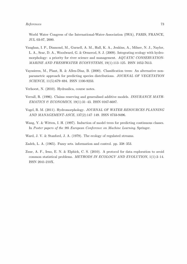
References 73
World Water Congress of the International-Water-Association (IWA), PARIS, FRANCE,
JUL 03-07, 2000.
Vaughan, I. P., Diamond, M., Gurnell, A. M., Hall, K. A., Jenkins, A., Milner, N. J., Naylor,
L. A., Sear, D. A., Woodward, G. & Ormerod, S. J. (2009). Integrating ecology with hydro-
morphology: a priority for river science and management. AQUATIC CONSERVATION-
MARINE AND FRESHWATER ECOSYSTEMS, 19(1):113–125. ISSN 1052-7613.
Vayssieres, M., Plant, R. & Allen-Diaz, B. (2000). Classification trees: An alternative non-
parametric approach for predicting species distributions. JOURNAL OF VEGETATION
SCIENCE, 11(5):679–694. ISSN 1100-9233.
Verhoest, N. (2010). Hydraulica, course notes.
Verrall, R. (1996). Claims reserving and generalised additive models. INSURANCE MATH-
EMATICS & ECONOMICS, 19(1):31–43. ISSN 0167-6687.
Vogel, R. M. (2011). Hydromorphology. JOURNAL OF WATER RESOURCES PLANNING
AND MANAGEMENT-ASCE, 137(2):147–149. ISSN 0733-9496.
Wang, Y. & Witten, I. H. (1997). Induction of model trees for predicting continuous classes.
In Poster papers of the 9th European Conference on Machine Learning. Springer.
Ward, J. V. & Stanford, J. A. (1979). The ecology of regulated streams.
Zadeh, L. A. (1965). Fuzzy sets. information and control. pp. 338–353.
Zuur, A. F., Ieno, E. N. & Elphick, C. S. (2010). A protocol for data exploration to avoid
common statistical problems. METHODS IN ECOLOGY AND EVOLUTION, 1(1):3–14.
ISSN 2041-210X.
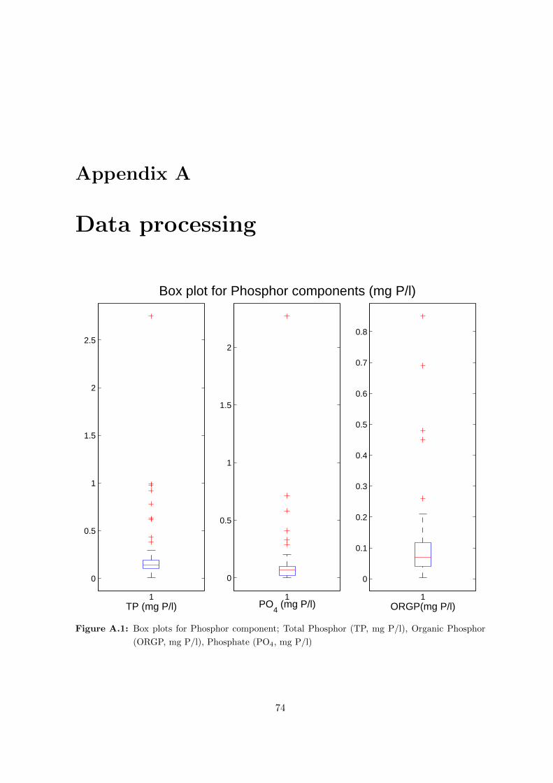
Appendix A
Data processing
0
0.5
1
1.5
2
2.5
1TP (mg P/l)
0
0.5
1
1.5
2
1PO
4 (mg P/l)
Box plot for Phosphor components (mg P/l)
0
0.1
0.2
0.3
0.4
0.5
0.6
0.7
0.8
1ORGP(mg P/l)
Figure A.1: Box plots for Phosphor component; Total Phosphor (TP, mg P/l), Organic Phosphor
(ORGP, mg P/l), Phosphate (PO4, mg P/l)
74
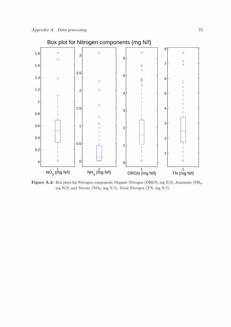
Appendix A. Data processing 75
0
0.2
0.4
0.6
0.8
1
1.2
1.4
1.6
1.8
1NO
3 (mg N/l)
0
0.5
1
1.5
2
2.5
3
1NH
4 (mg N/l)
Box plot for Nitrogen components (mg N/l)
0
1
2
3
4
5
6
1ORGN (mg N/l)
1
2
3
4
5
6
7
8
1TN (mg N/l)
Figure A.2: Box plots for Nitrogen component; Organic Nitrogen (ORGN, mg N/l), Ammonia (NH4,
mg N/l) and Nitrate (NO3, mg N/l), Total Nitrogen (TN, mg N/l)
Appendix A. Data processing 76
0
5
10
15
20
25
30
35
40
45
1TSS (mg/l)
0
10
20
30
40
50
1BOD
5 (mg O
2/l)
Box plot for TSS (mg/l), BOD and COD (mg O2/l) components
0
50
100
150
200
250
300
350
400
450
1COD (mg O
2/l)
Figure A.3: Box plots for Total Suspended Solids (TSS, mg/l), Chemical Oxygen Demand (DO, mg
O2/l) and Biological Oxygen Demand(BOD, BOD5 mg O2/l)
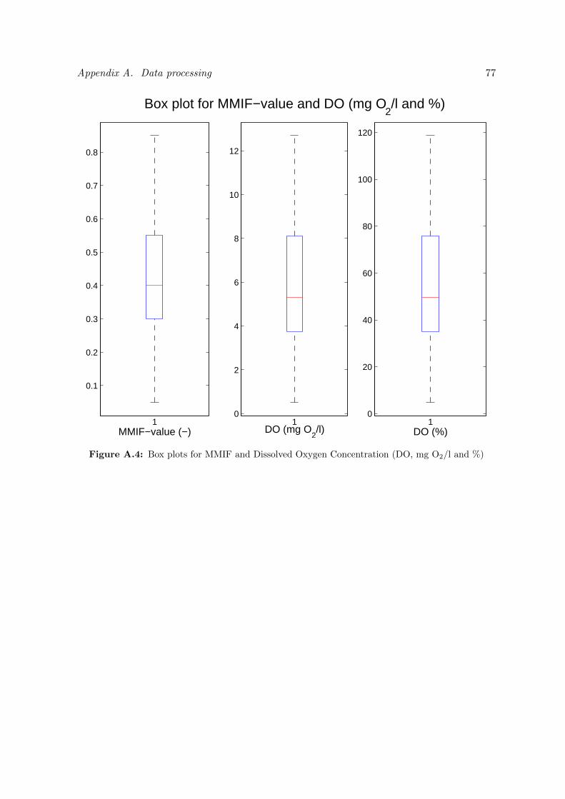
Appendix A. Data processing 77
0.1
0.2
0.3
0.4
0.5
0.6
0.7
0.8
1MMIF−value (−)
0
2
4
6
8
10
12
1DO (mg O
2/l)
Box plot for MMIF−value and DO (mg O2/l and %)
0
20
40
60
80
100
120
1DO (%)
Figure A.4: Box plots for MMIF and Dissolved Oxygen Concentration (DO, mg O2/l and %)
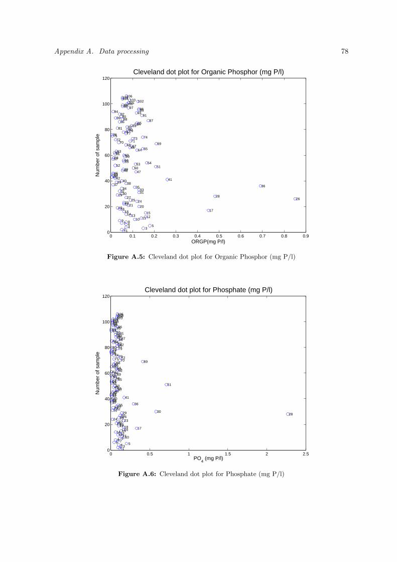
Appendix A. Data processing 78
0 0.1 0.2 0.3 0.4 0.5 0.6 0.7 0.8 0.90
20
40
60
80
100
120Cleveland dot plot for Organic Phosphor (mg P/l)
ORGP(mg P/l)
Num
ber
of s
ampl
e
1 2 3 4 5 6 7 8 9 10 11 12 13 14 15 16 17 18 19 20 21 22 23 24 25 26 27 28 29 30 31 32 33 34 35 36 37 38 39 40 41 42 43 44 45 46 47 48 49 50 51 52 53 54 55 56 57 58 59 60 61 62 63 64 65 66 67 68 69 70 71 72 73 74 75 76 77 78 79 80 81 82 83 84 85 86 87 88 89 90 91 92 93 94 95 96 97 98 99100101 102103104105106
Figure A.5: Cleveland dot plot for Organic Phosphor (mg P/l)
0 0.5 1 1.5 2 2.50
20
40
60
80
100
120Cleveland dot plot for Phosphate (mg P/l)
PO4 (mg P/l)
Num
ber
of s
ampl
e
1 2 3 4 5 6 7 8 9 10 11 12 13 14 15 16 17 18 19 20 21 22 23 24 25 26 27 28 29 30 31 32 33 34 35 36 37 38 39 40 41 42 43 44 45 46 47 48 49 50 51 52 53 54 55 56 57 58 59 60 61 62 63 64 65 66 67 68 69 70 71 72 73 74 75 76 77 78 79 80 81 82 83 84 85 86 87 88 89 90 91 92 93 94 95 96 97 98 99100101102103104105106
Figure A.6: Cleveland dot plot for Phosphate (mg P/l)
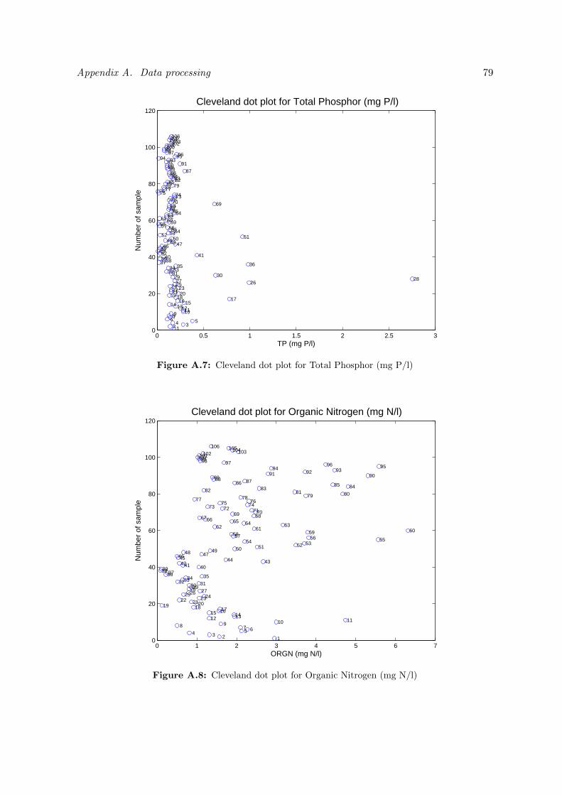
Appendix A. Data processing 79
0 0.5 1 1.5 2 2.5 30
20
40
60
80
100
120Cleveland dot plot for Total Phosphor (mg P/l)
TP (mg P/l)
Num
ber
of s
ampl
e
1 2 3 4 5 6 7 8 9
10 11 12 13 14 15 16 17 18 19 20 21 22 23 24 25 26 27 28 29 30 31 32 33 34 35 36 37 38 39 40 41 42 43 44 45 46 47 48 49 50 51 52 53 54 55 56 57 58 59 60 61 62 63 64 65 66 67 68 69 70 71 72 73 74 75 76 77 78 79 80 81 82 83 84 85 86 87 88 89 90 91 92 93 94 95 96 97 98 99100101102103104105106
Figure A.7: Cleveland dot plot for Total Phosphor (mg P/l)
0 1 2 3 4 5 6 70
20
40
60
80
100
120Cleveland dot plot for Organic Nitrogen (mg N/l)
ORGN (mg N/l)
Num
ber
of s
ampl
e
1 2 3 4 5 6 7 8 9 10 11 12 13 14 15 16 17 18 19 20 21 22 23 24 25 26 27 28 29 30 31 32 33 34 35 36 37 38 39 40 41 42 43 44 45 46 47 48 49 50 51 52 53 54 55 56 57 58 59 60 61 62 63 64 65 66 67 68 69 70 71 72 73 74 75 76 77 78 79 80 81 82 83 84 85 86 87 88 89 90 91 92 93 94 95 96 97 98 99100101102 103104105106
Figure A.8: Cleveland dot plot for Organic Nitrogen (mg N/l)
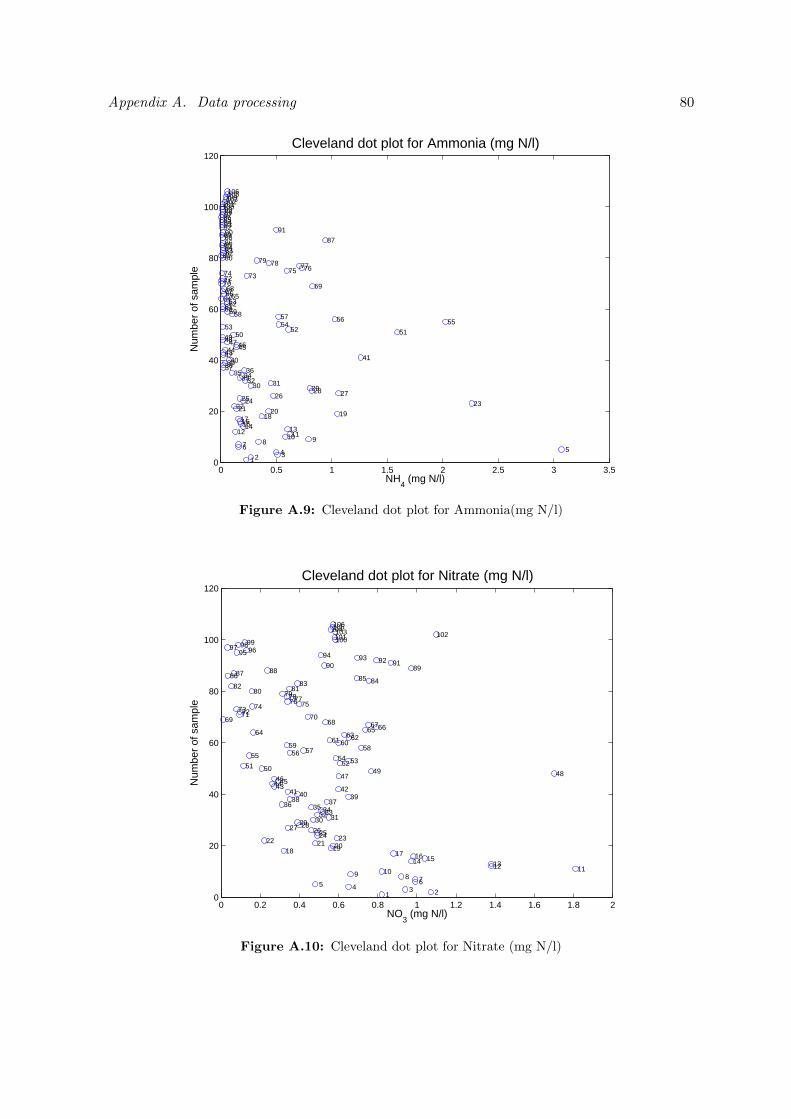
Appendix A. Data processing 80
0 0.5 1 1.5 2 2.5 3 3.50
20
40
60
80
100
120Cleveland dot plot for Ammonia (mg N/l)
NH4 (mg N/l)
Num
ber
of s
ampl
e
1 2 3 4 5 6 7 8 9 10 11 12 13 14 15 16 17 18 19 20 21 22 23 24 25 26 27 28 29 30 31 32 33 34 35 36 37 38 39 40 41 42 43 44 45 46 47 48 49 50 51 52 53 54 55 56 57 58 59 60 61 62 63 64 65 66 67 68 69 70 71 72 73 74 75 76 77 78 79 80 81 82 83 84 85 86 87 88 89 90 91 92 93 94 95 96 97 98 99100101102103104105106
Figure A.9: Cleveland dot plot for Ammonia(mg N/l)
0 0.2 0.4 0.6 0.8 1 1.2 1.4 1.6 1.8 20
20
40
60
80
100
120Cleveland dot plot for Nitrate (mg N/l)
NO3 (mg N/l)
Num
ber
of s
ampl
e
1 2 3 4 5 6 7 8 9 10 11 12 13 14 15 16 17 18 19 20 21 22 23 24 25 26 27 28 29 30 31 32 33 34 35 36 37 38 39 40 41 42 43 44 45 46 47 48 49 50 51 52 53 54 55 56 57 58 59 60 61 62 63 64 65 66 67 68 69 70 71 72 73 74 75 76 77 78 79 80 81 82 83 84 85 86 87 88 89 90 91 92 93 94 95 96 97 98 99 100101 102103104105106
Figure A.10: Cleveland dot plot for Nitrate (mg N/l)
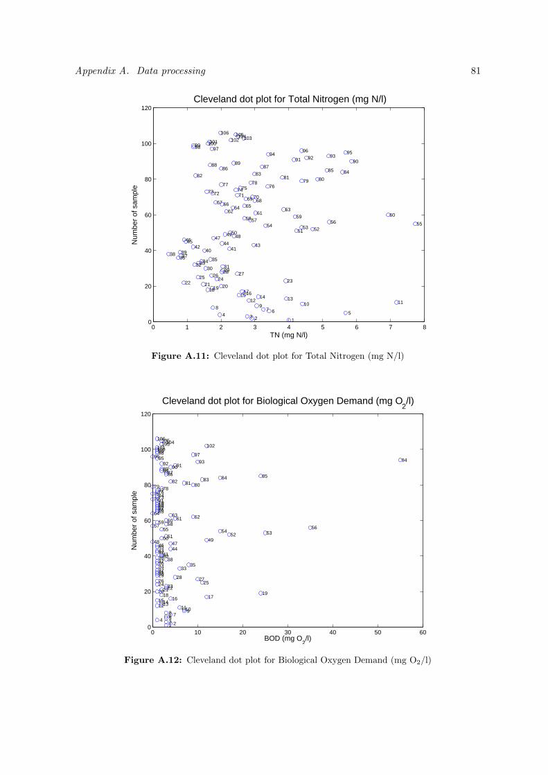
Appendix A. Data processing 81
0 1 2 3 4 5 6 7 80
20
40
60
80
100
120Cleveland dot plot for Total Nitrogen (mg N/l)
TN (mg N/l)
Num
ber
of s
ampl
e
1 2 3 4 5 6 7 8 9 10 11 12 13 14 15 16 17 18 19 20 21 22 23 24 25 26 27 28 29 30 31 32 33 34 35 36 37 38 39 40 41 42 43 44 45 46 47 48 49 50 51 52 53 54 55 56 57 58 59 60 61 62 63 64 65 66 67 68 69 70 71 72 73 74 75 76 77 78 79 80 81 82 83 84 85 86 87 88 89 90 91 92 93 94 95 96 97 98 99 100101 102 103104105106
Figure A.11: Cleveland dot plot for Total Nitrogen (mg N/l)
0 10 20 30 40 50 600
20
40
60
80
100
120
Cleveland dot plot for Biological Oxygen Demand (mg O2/l)
BOD (mg O2/l)
Num
ber
of s
ampl
e
1 2 3 4 5 6 7 8 9 10 11 12 13 14 15 16 17 18 19 20 21 22 23 24 25 26 27 28 29 30 31 32 33 34 35 36 37 38 39 40 41 42 43 44 45 46 47 48 49 50 51 52 53 54 55 56 57 58 59 60 61 62 63 64 65 66 67 68 69 70 71 72 73 74 75 76 77 78 79 80 81 82 83 84 85 86 87 88 89 90 91 92 93 94 95 96 97 98 99100101 102103104105106
Figure A.12: Cleveland dot plot for Biological Oxygen Demand (mg O2/l)
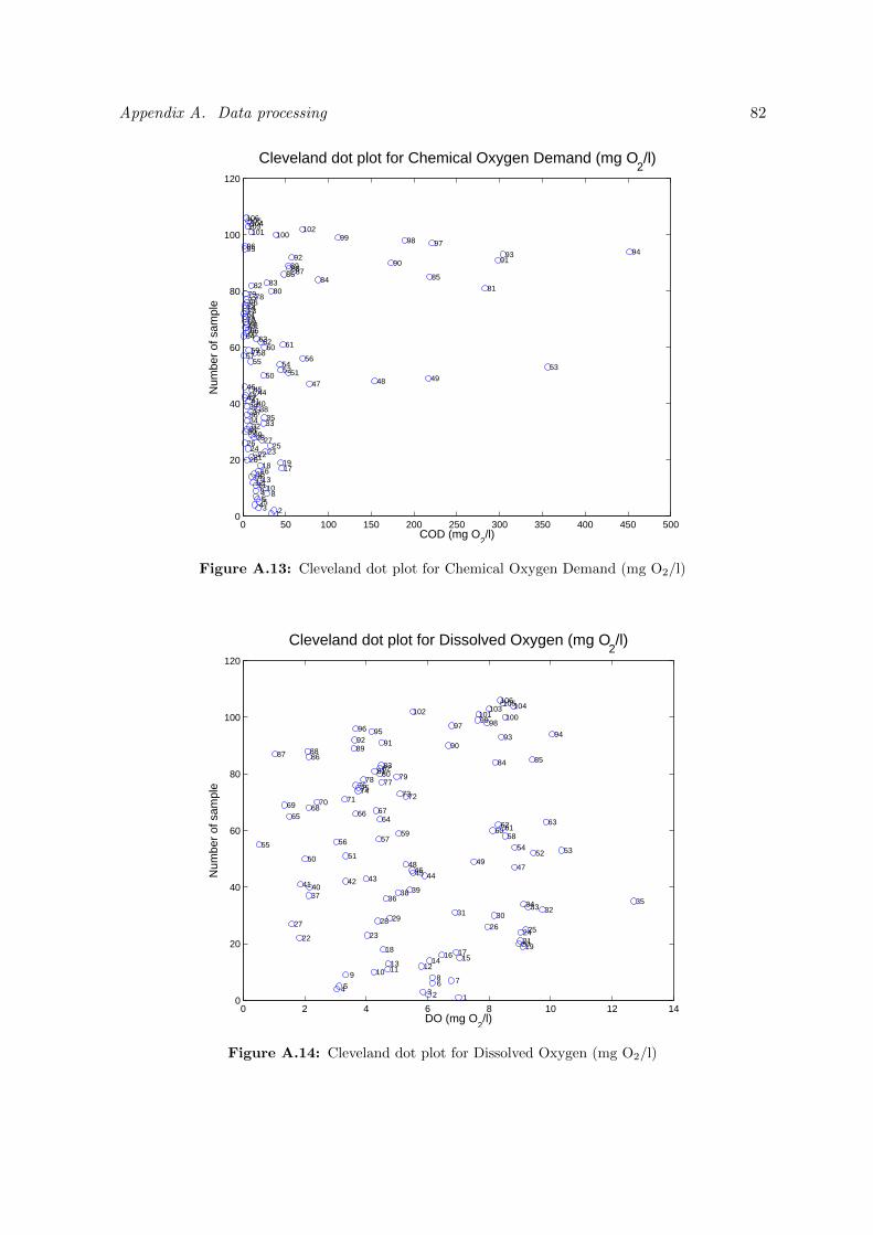
Appendix A. Data processing 82
0 50 100 150 200 250 300 350 400 450 5000
20
40
60
80
100
120
Cleveland dot plot for Chemical Oxygen Demand (mg O2/l)
COD (mg O2/l)
Num
ber
of s
ampl
e
1 2 3 4 5 6 7 8 9 10 11 12 13 14 15 16 17 18 19 20 21 22 23 24 25 26 27 28 29 30 31 32 33 34 35 36 37 38 39 40 41 42 43 44 45 46 47 48 49 50 51 52 53 54 55 56 57 58 59 60 61 62 63 64 65 66 67 68 69 70 71 72 73 74 75 76 77 78 79 80 81 82 83 84 85 86 87 88 89 90 91 92 93 94 95 96 97 98 99100101 102103104105106
Figure A.13: Cleveland dot plot for Chemical Oxygen Demand (mg O2/l)
0 2 4 6 8 10 12 140
20
40
60
80
100
120
DO (mg O2/l)
Cleveland dot plot for Dissolved Oxygen (mg O2/l)
Num
ber
of s
ampl
e
1 2 3 4 5 6 7 8 9 10 11 12 13 14 15 16 17 18 19 20 21 22 23 24 25 26 27 28 29 30 31 32 33 34 35 36 37 38 39 40 41 42 43 44 45 46 47 48 49 50 51 52 53 54 55 56 57 58 59 60 61 62 63 64 65 66 67 68 69 70 71 72 73 74 75 76 77 78 79 80 81 82 83 84 85 86 87 88 89 90 91 92 93 94 95 96 97 98 99 100101102 103 104105106
Figure A.14: Cleveland dot plot for Dissolved Oxygen (mg O2/l)
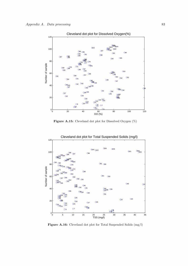
Appendix A. Data processing 83
0 20 40 60 80 100 1200
20
40
60
80
100
120Cleveland dot plot for Dissolved Oxygen(%)
DO (%)
Num
ber
of s
ampl
e
1 2 3 4 5 6 7 8 9 10 11 12 13 14 15 16 17 18 19 20 21 22 23 24 25 26 27 28 29 30 31 32 33 34 35 36 37 38 39 40 41 42 43 44 45 46 47 48 49 50 51 52 53 54 55 56 57 58 59 60 61 62 63 64 65 66 67 68 69 70 71 72 73 74 75 76 77 78 79 80 81 82 83 84 85 86 87 88 89 90 91 92 93 94 95 96 97 98 99 100101102 103 104105106
Figure A.15: Cleveland dot plot for Dissolved Oxygen (%)
0 5 10 15 20 25 30 35 40 450
20
40
60
80
100
120Cleveland dot plot for Total Suspended Solids (mg/l)
TSS (mg/l)
Num
ber
of s
ampl
e
1 2 3 4 5 6 7 8 9 10 11 12 13 14 15 16 17 18 19 20 21 22 23 24 25 26 27 28 29 30 31 32 33 34 35 36 37 38 39 40 41 42 43 44 45 46 47 48 49 50 51 52 53 54 55 56 57 58 59 60 61 62 63 64 65 66 67 68 69 70 71 72 73 74 75 76 77 78 79 80 81 82 83 84 85 86 87 88 89 90 91 92 93 94 95 96 97 98 99 100101 102103104 105106
Figure A.16: Cleveland dot plot for Total Suspended Solids (mg/l)
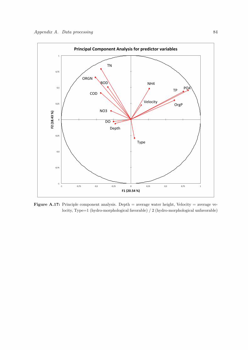
Appendix A. Data processing 84
DO
BOD
NO3
PO4 NH4
Depth
Velocity OrgP
ORGN
Type
COD
TN
TP
‐1
‐0,75
‐0,5
‐0,25
0
0,25
0,5
0,75
1
‐1 ‐0,75 ‐0,5 ‐0,25 0 0,25 0,5 0,75 1
F2 (1
8.43
%)
F1 (20.54 %)
Principal Component Analysis for predictor variables
Figure A.17: Principle component analysis. Depth = average water height, Velocity = average ve-
locity, Type=1 (hydro-morphological favorable) / 2 (hydro-morphological unfavorable)
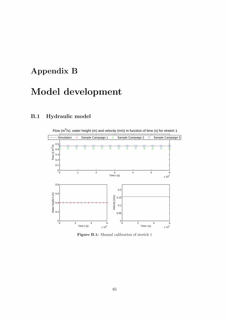
Appendix B
Model development
B.1 Hydraulic model
0 1 2 3 4 5 6
x 105
0
0.1
0.2
0.3
0.4
0.5
0.6
Time t (s)
Flo
w Q
(m
3 /s)
Flow (m3/s), water height (m) and velocity (m/s) in function of time (s) for stretch 1
Simulation Sample Campaign 1 Sample Campaign 2 Sample Campaign 3
0 2 4 6
x 105
0
0.2
0.4
0.6
0.8
Wat
er h
eigh
t h (
m)
Time t (s)0 2 4 6
x 105
0
0.05
0.1
0.15
0.2
Vel
ocity
(m
/s)
Time t (s)
Figure B.1: Manual calibration of stretch 1
85
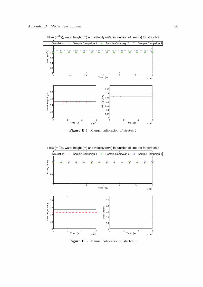
Appendix B. Model development 86
0 1 2 3 4 5 6
x 105
0
0.2
0.4
0.6
0.8
1
1.2
Time t (s)
Flo
w Q
(m
3 /s)
Flow (m3/s), water height (m) and velocity (m/s) in function of time (s) for stretch 2
Simulation Sample Campaign 1 Sample Campaign 2 Sample Campaign 3
0 2 4 6
x 105
0
0.2
0.4
0.6
0.8
1
Wat
er h
eigh
t h (
m)
Time t (s)0 2 4 6
x 105
0
0.05
0.1
0.15
0.2
0.25
0.3
0.35
Vel
ocity
(m
/s)
Time t (s)
Figure B.2: Manual calibration of stretch 2
0 1 2 3 4 5 6
x 105
0
0.5
1
1.5
Time t (s)
Flo
w Q
(m
3 /s)
Flow (m3/s), water height (m) and velocity (m/s) in function of time (s) for stretch 3
Simulation Sample Campaign 1 Sample Campaign 2 Sample Campaign 3
0 2 4 6
x 105
0
0.2
0.4
0.6
0.8
Wat
er h
eigh
t h (
m)
Time t (s)0 2 4 6
x 105
0
0.1
0.2
0.3
0.4
0.5
Vel
ocity
(m
/s)
Time t (s)
Figure B.3: Manual calibration of stretch 3
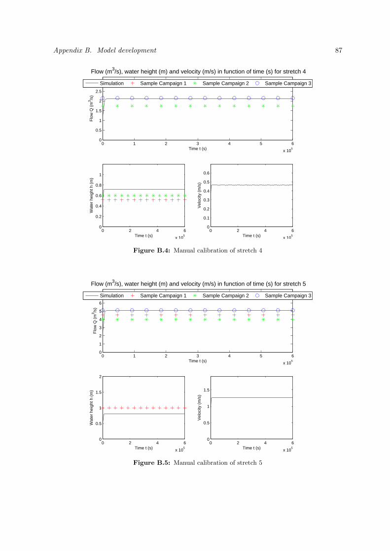
Appendix B. Model development 87
0 1 2 3 4 5 6
x 105
0
0.5
1
1.5
2
2.5
3
Time t (s)
Flo
w Q
(m
3 /s)
Flow (m3/s), water height (m) and velocity (m/s) in function of time (s) for stretch 4
Simulation Sample Campaign 1 Sample Campaign 2 Sample Campaign 3
0 2 4 6
x 105
0
0.2
0.4
0.6
0.8
1
Wat
er h
eigh
t h (
m)
Time t (s)0 2 4 6
x 105
0
0.1
0.2
0.3
0.4
0.5
0.6
Vel
ocity
(m
/s)
Time t (s)
Figure B.4: Manual calibration of stretch 4
0 1 2 3 4 5 6
x 105
0
1
2
3
4
5
6
7
Time t (s)
Flo
w Q
(m
3 /s)
Flow (m3/s), water height (m) and velocity (m/s) in function of time (s) for stretch 5
Simulation Sample Campaign 1 Sample Campaign 2 Sample Campaign 3
0 2 4 6
x 105
0
0.5
1
1.5
2
Wat
er h
eigh
t h (
m)
Time t (s)0 2 4 6
x 105
0
0.5
1
1.5
Vel
ocity
(m
/s)
Time t (s)
Figure B.5: Manual calibration of stretch 5
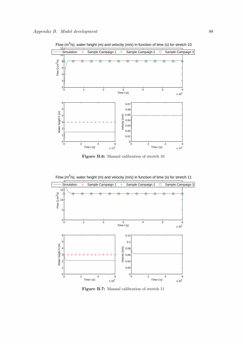
Appendix B. Model development 88
0 1 2 3 4 5 6
x 105
0
2
4
6
8
10
12
Time t (s)
Flo
w Q
(m
3 /s)
Flow (m3/s), water height (m) and velocity (m/s) in function of time (s) for stretch 10
Simulation Sample Campaign 1 Sample Campaign 2 Sample Campaign 3
0 2 4 6
x 105
0
1
2
3
4
5
6
Wat
er h
eigh
t h (
m)
Time t (s)0 2 4 6
x 105
0
0.01
0.02
0.03
0.04
0.05
0.06
0.07
Vel
ocity
(m
/s)
Time t (s)
Figure B.6: Manual calibration of stretch 10
0 1 2 3 4 5 6
x 105
0
5
10
15
Time t (s)
Flo
w Q
(m
3 /s)
Flow (m3/s), water height (m) and velocity (m/s) in function of time (s) for stretch 11
Simulation Sample Campaign 1 Sample Campaign 2 Sample Campaign 3
0 2 4 6
x 105
0
1
2
3
4
5
6
Wat
er h
eigh
t h (
m)
Time t (s)0 2 4 6
x 105
0
0.02
0.04
0.06
0.08
0.1
0.12
Vel
ocity
(m
/s)
Time t (s)
Figure B.7: Manual calibration of stretch 11

Appendix B. Model development 89
0 1 2 3 4 5 6
x 105
0
5
10
15
Time t (s)
Flo
w Q
(m
3 /s)
Flow (m3/s), water height (m) and velocity (m/s) in function of time (s) for stretch 12
Simulation Sample Campaign 1 Sample Campaign 2 Sample Campaign 3
0 2 4 6
x 105
0
0.1
0.2
0.3
0.4
Wat
er h
eigh
t h (
m)
Time t (s)0 2 4 6
x 105
0
0.2
0.4
0.6
0.8
Vel
ocity
(m
/s)
Time t (s)
Figure B.8: Manual calibration of stretch 12
0 1 2 3 4 5 6
x 105
0
5
10
15
Time t (s)
Flo
w Q
(m
3 /s)
Flow (m3/s), water height (m) and velocity (m/s) in function of time (s) for stretch 13
Simulation Sample Campaign 1 Sample Campaign 2 Sample Campaign 3
0 2 4 6
x 105
0
1
2
3
4
5
6
Wat
er h
eigh
t h (
m)
Time t (s)0 2 4 6
x 105
0
0.01
0.02
0.03
0.04
0.05
0.06
Vel
ocity
(m
/s)
Time t (s)
Figure B.9: Manual calibration of stretch 13

Appendix B. Model development 90
0 1 2 3 4 5 6
x 105
0
5
10
15
Time t (s)
Flo
w Q
(m
3 /s)
Flow (m3/s), water height (m) and velocity (m/s) in function of time (s) for stretch 14
Simulation Sample Campaign 1 Sample Campaign 2 Sample Campaign 3
0 2 4 6
x 105
0
0.1
0.2
0.3
0.4
Wat
er h
eigh
t h (
m)
Time t (s)0 2 4 6
x 105
0
0.2
0.4
0.6
0.8
Vel
ocity
(m
/s)
Time t (s)
Figure B.10: Manual calibration of stretch 14
0 1 2 3 4 5 6
x 105
0
5
10
15
Time t (s)
Flo
w Q
(m
3 /s)
Flow (m3/s), water height (m) and velocity (m/s) in function of time (s) for stretch 15
Simulation Sample Campaign 1 Sample Campaign 2 Sample Campaign 3
0 2 4 6
x 105
0
1
2
3
4
5
6
Wat
er h
eigh
t h (
m)
Time t (s)0 2 4 6
x 105
0
0.01
0.02
0.03
0.04
0.05
0.06
Vel
ocity
(m
/s)
Time t (s)
Figure B.11: Manual calibration of stretch 15
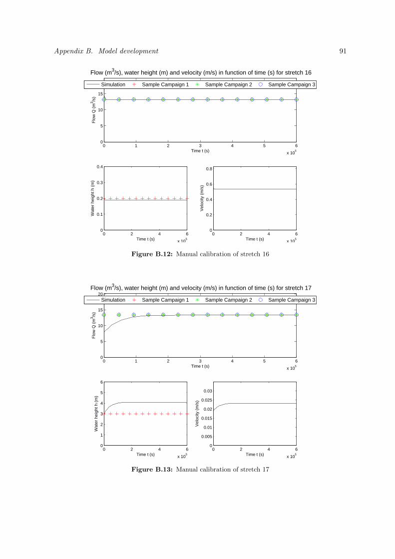
Appendix B. Model development 91
0 1 2 3 4 5 6
x 105
0
5
10
15
Time t (s)
Flo
w Q
(m
3 /s)
Flow (m3/s), water height (m) and velocity (m/s) in function of time (s) for stretch 16
Simulation Sample Campaign 1 Sample Campaign 2 Sample Campaign 3
0 2 4 6
x 105
0
0.1
0.2
0.3
0.4
Wat
er h
eigh
t h (
m)
Time t (s)0 2 4 6
x 105
0
0.2
0.4
0.6
0.8
Vel
ocity
(m
/s)
Time t (s)
Figure B.12: Manual calibration of stretch 16
0 1 2 3 4 5 6
x 105
0
5
10
15
20
Time t (s)
Flo
w Q
(m
3 /s)
Flow (m3/s), water height (m) and velocity (m/s) in function of time (s) for stretch 17
Simulation Sample Campaign 1 Sample Campaign 2 Sample Campaign 3
0 2 4 6
x 105
0
1
2
3
4
5
6
Wat
er h
eigh
t h (
m)
Time t (s)0 2 4 6
x 105
0
0.005
0.01
0.015
0.02
0.025
0.03
Vel
ocity
(m
/s)
Time t (s)
Figure B.13: Manual calibration of stretch 17
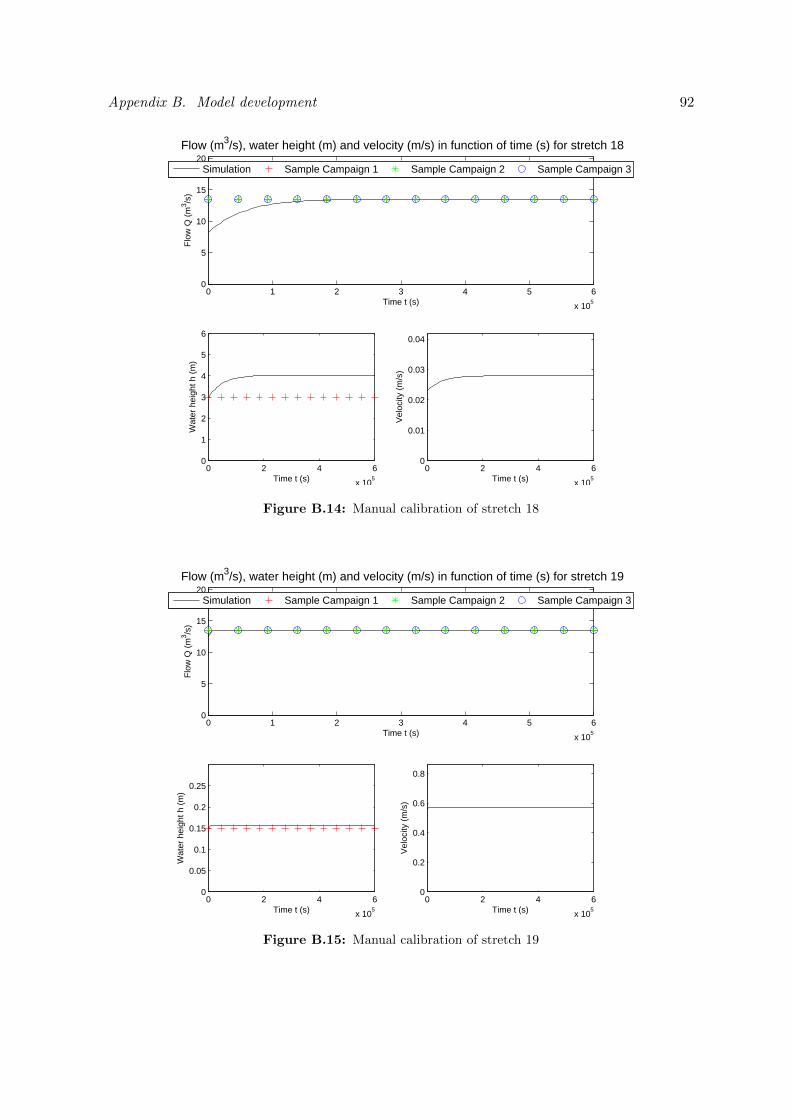
Appendix B. Model development 92
0 1 2 3 4 5 6
x 105
0
5
10
15
20
Time t (s)
Flo
w Q
(m
3 /s)
Flow (m3/s), water height (m) and velocity (m/s) in function of time (s) for stretch 18
Simulation Sample Campaign 1 Sample Campaign 2 Sample Campaign 3
0 2 4 6
x 105
0
1
2
3
4
5
6
Wat
er h
eigh
t h (
m)
Time t (s)0 2 4 6
x 105
0
0.01
0.02
0.03
0.04
Vel
ocity
(m
/s)
Time t (s)
Figure B.14: Manual calibration of stretch 18
0 1 2 3 4 5 6
x 105
0
5
10
15
20
Time t (s)
Flo
w Q
(m
3 /s)
Flow (m3/s), water height (m) and velocity (m/s) in function of time (s) for stretch 19
Simulation Sample Campaign 1 Sample Campaign 2 Sample Campaign 3
0 2 4 6
x 105
0
0.05
0.1
0.15
0.2
0.25
Wat
er h
eigh
t h (
m)
Time t (s)0 2 4 6
x 105
0
0.2
0.4
0.6
0.8
Vel
ocity
(m
/s)
Time t (s)
Figure B.15: Manual calibration of stretch 19
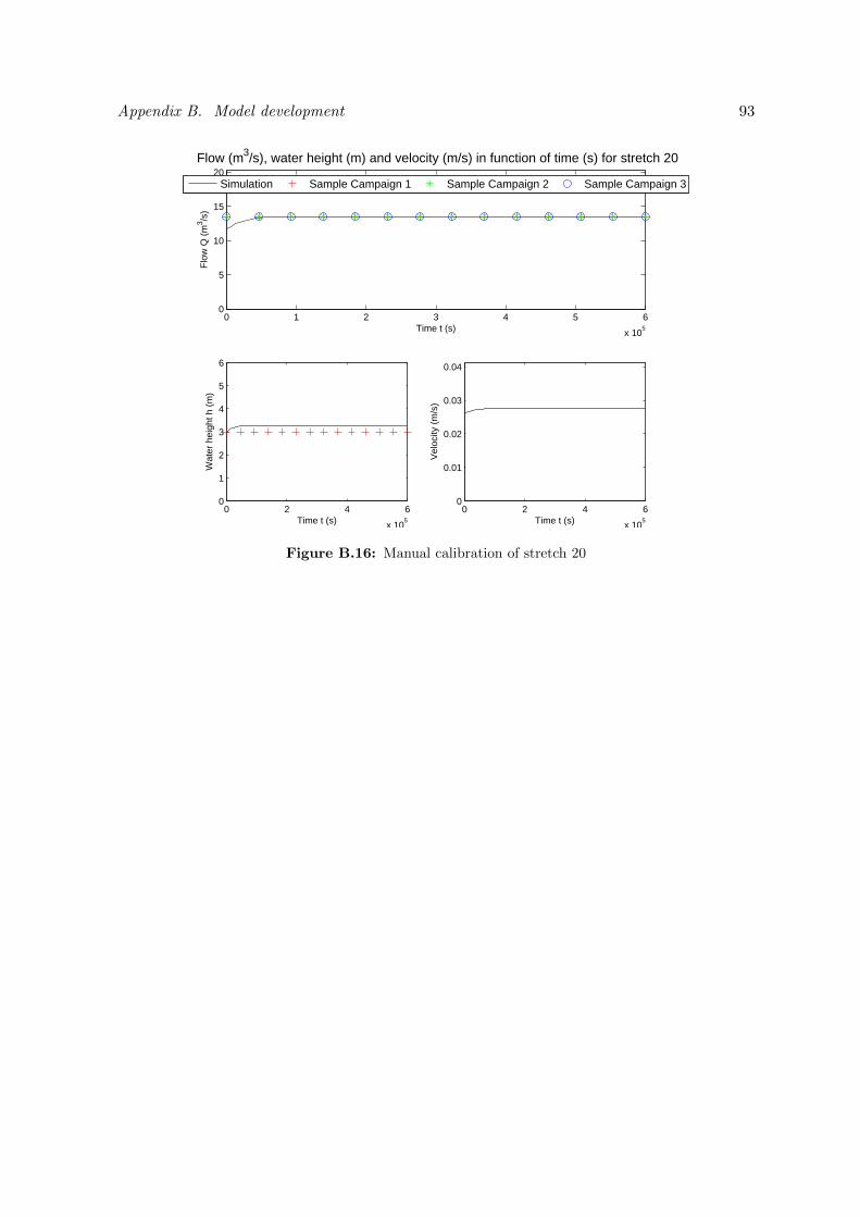
Appendix B. Model development 93
0 1 2 3 4 5 6
x 105
0
5
10
15
20
Time t (s)
Flo
w Q
(m
3 /s)
Flow (m3/s), water height (m) and velocity (m/s) in function of time (s) for stretch 20
Simulation Sample Campaign 1 Sample Campaign 2 Sample Campaign 3
0 2 4 6
x 105
0
1
2
3
4
5
6
Wat
er h
eigh
t h (
m)
Time t (s)0 2 4 6
x 105
0
0.01
0.02
0.03
0.04
Vel
ocity
(m
/s)
Time t (s)
Figure B.16: Manual calibration of stretch 20
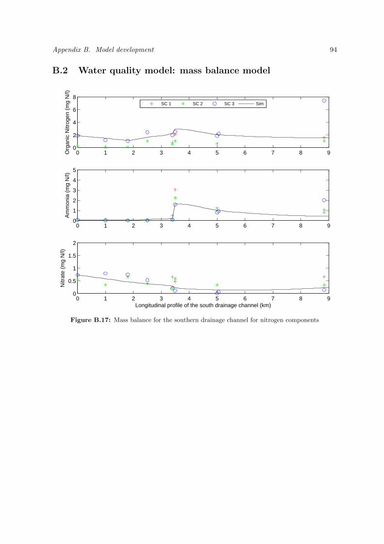
Appendix B. Model development 94
B.2 Water quality model: mass balance model
0 1 2 3 4 5 6 7 8 90
2
4
6
8
Org
anic
Nitr
ogen
(m
g N
/l)
SC 1 SC 2 SC 3 Sim
0 1 2 3 4 5 6 7 8 90
1
2
3
4
5
Am
mon
ia (
mg
N/l)
0 1 2 3 4 5 6 7 8 90
0.5
1
1.5
2
Nitr
ate
(mg
N/l)
Longitudinal profile of the south drainage channel (km)
Figure B.17: Mass balance for the southern drainage channel for nitrogen components
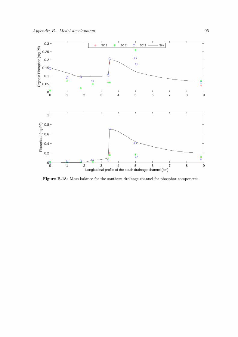
Appendix B. Model development 95
0 1 2 3 4 5 6 7 8 90
0.05
0.1
0.15
0.2
0.25
0.3
Org
anic
Pho
spho
r (m
g P
/l)
SC 1 SC 2 SC 3 Sim
0 1 2 3 4 5 6 7 8 90
0.2
0.4
0.6
0.8
1
Pho
spha
te (
mg
P/l)
Longitudinal profile of the south drainage channel (km)
Figure B.18: Mass balance for the southern drainage channel for phosphor components
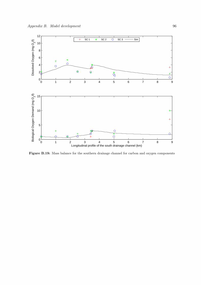
Appendix B. Model development 96
0 1 2 3 4 5 6 7 8 90
2
4
6
8
10
12D
isso
lved
Oxy
gen
(mg
O2/l)
SC 1 SC 2 SC 3 Sim
0 1 2 3 4 5 6 7 8 90
5
10
15
Bio
logi
cal O
xyge
n D
eman
d (m
g O
2/l)
Longitudinal profile of the south drainage channel (km)
Figure B.19: Mass balance for the southern drainage channel for carbon and oxygen components
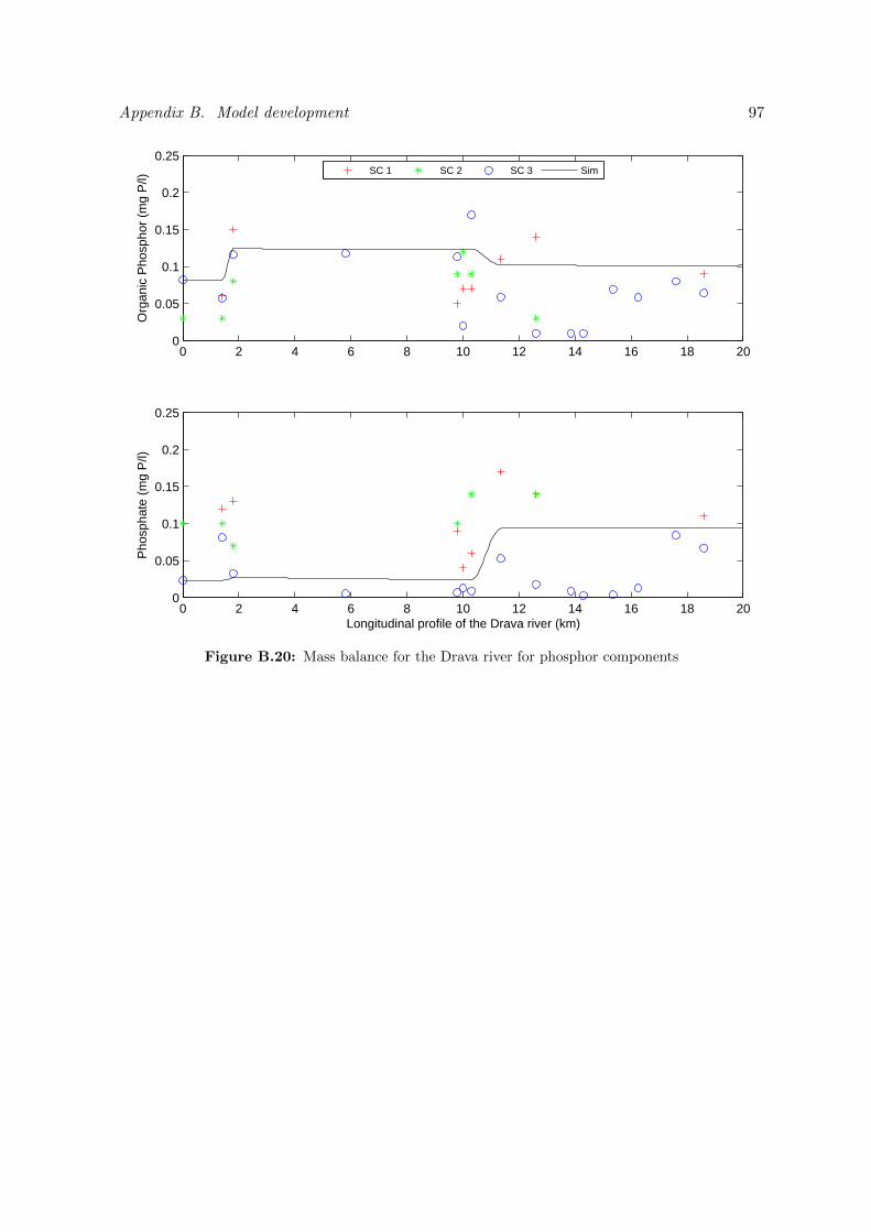
Appendix B. Model development 97
0 2 4 6 8 10 12 14 16 18 200
0.05
0.1
0.15
0.2
0.25O
rgan
ic P
hosp
hor
(mg
P/l)
SC 1 SC 2 SC 3 Sim
0 2 4 6 8 10 12 14 16 18 200
0.05
0.1
0.15
0.2
0.25
Pho
spha
te (
mg
P/l)
Longitudinal profile of the Drava river (km)
Figure B.20: Mass balance for the Drava river for phosphor components
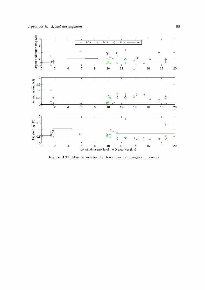
Appendix B. Model development 98
0 2 4 6 8 10 12 14 16 18 200
2
4
6
8O
rgan
ic N
itrog
en (
mg
N/l)
SC 1 SC 2 SC 3 Sim
0 2 4 6 8 10 12 14 16 18 200
0.5
1
1.5
2
Am
mon
ia (
mg
N/l)
0 2 4 6 8 10 12 14 16 18 200
0.5
1
1.5
2
Nitr
ate
(mg
N/l)
Longitudinal profile of the Drava river (km)
Figure B.21: Mass balance for the Drava river for nitrogen components
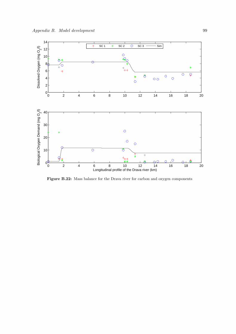
Appendix B. Model development 99
0 2 4 6 8 10 12 14 16 18 200
2
4
6
8
10
12
14D
isso
lved
Oxy
gen
(mg
O2/l)
SC 1 SC 2 SC 3 Sim
0 2 4 6 8 10 12 14 16 18 200
10
20
30
40
Bio
logi
cal O
xyge
n D
eman
d (m
g O
2/l)
Longitudinal profile of the Drava river (km)
Figure B.22: Mass balance for the Drava river for carbon and oxygen components
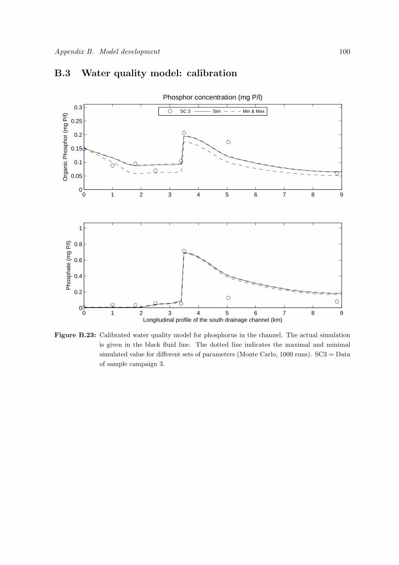
Appendix B. Model development 100
B.3 Water quality model: calibration
0 1 2 3 4 5 6 7 8 90
0.05
0.1
0.15
0.2
0.25
0.3
Phosphor concentration (mg P/l)
Org
anic
Pho
spho
r (m
g P
/l)
SC 3 Sim Min & Max
0 1 2 3 4 5 6 7 8 90
0.2
0.4
0.6
0.8
1
Pho
spha
te (
mg
P/l)
Longitudinal profile of the south drainage channel (km)
Figure B.23: Calibrated water quality model for phosphorus in the channel. The actual simulation
is given in the black fluid line. The dotted line indicates the maximal and minimal
simulated value for different sets of parameters (Monte Carlo, 1000 runs). SC3 = Data
of sample campaign 3.
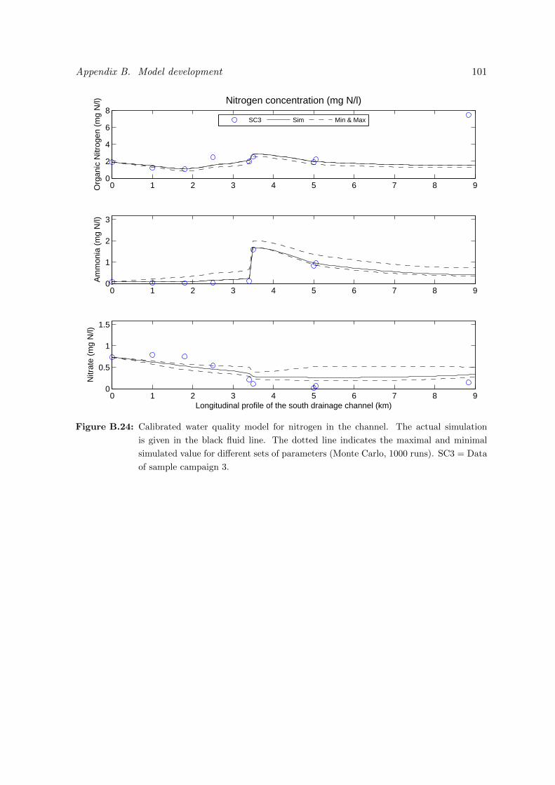
Appendix B. Model development 101
0 1 2 3 4 5 6 7 8 90
2
4
6
8Nitrogen concentration (mg N/l)
Org
anic
Nitr
ogen
(m
g N
/l)
SC3 Sim Min & Max
0 1 2 3 4 5 6 7 8 90
1
2
3
Am
mon
ia (
mg
N/l)
0 1 2 3 4 5 6 7 8 90
0.5
1
1.5
Nitr
ate
(mg
N/l)
Longitudinal profile of the south drainage channel (km)
Figure B.24: Calibrated water quality model for nitrogen in the channel. The actual simulation
is given in the black fluid line. The dotted line indicates the maximal and minimal
simulated value for different sets of parameters (Monte Carlo, 1000 runs). SC3 = Data
of sample campaign 3.
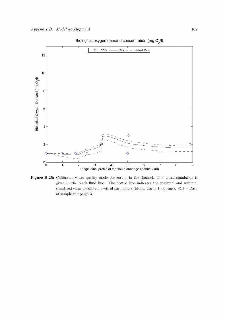
Appendix B. Model development 102
0 1 2 3 4 5 6 7 8 90
2
4
6
8
10
12
Biological oxygen demand concentration (mg O2/l)
Longitudinal profile of the south drainage channel (km)
Bio
logi
cal O
xyge
n D
eman
d (m
g O
2/l)
SC 3 Sim Min & Max
Figure B.25: Calibrated water quality model for carbon in the channel. The actual simulation is
given in the black fluid line. The dotted line indicates the maximal and minimal
simulated value for different sets of parameters (Monte Carlo, 1000 runs). SC3 = Data
of sample campaign 3.
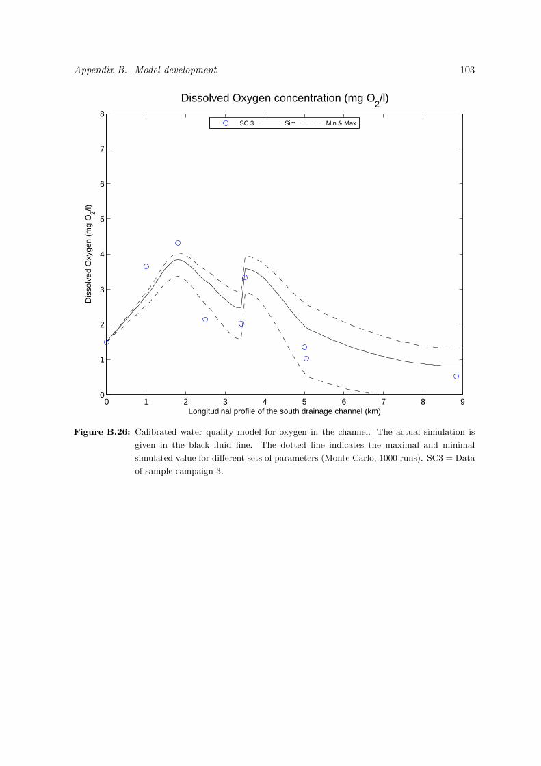
Appendix B. Model development 103
0 1 2 3 4 5 6 7 8 90
1
2
3
4
5
6
7
8
Dissolved Oxygen concentration (mg O2/l)
Longitudinal profile of the south drainage channel (km)
Dis
solv
ed O
xyge
n (m
g O
2/l)
SC 3 Sim Min & Max
Figure B.26: Calibrated water quality model for oxygen in the channel. The actual simulation is
given in the black fluid line. The dotted line indicates the maximal and minimal
simulated value for different sets of parameters (Monte Carlo, 1000 runs). SC3 = Data
of sample campaign 3.
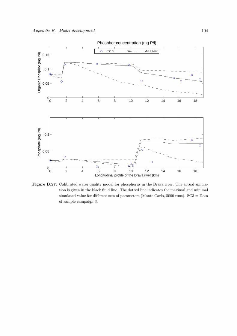
Appendix B. Model development 104
0 2 4 6 8 10 12 14 16 180
0.05
0.1
0.15
Phosphor concentration (mg P/l)O
rgan
ic P
hosp
hor
(mg
P/l)
SC 3 Sim Min & Max
0 2 4 6 8 10 12 14 16 180
0.05
0.1
Pho
spha
te (
mg
P/l)
Longitudinal profile of the Drava river (km)
Figure B.27: Calibrated water quality model for phosphorus in the Drava river. The actual simula-
tion is given in the black fluid line. The dotted line indicates the maximal and minimal
simulated value for different sets of parameters (Monte Carlo, 5000 runs). SC3 = Data
of sample campaign 3.
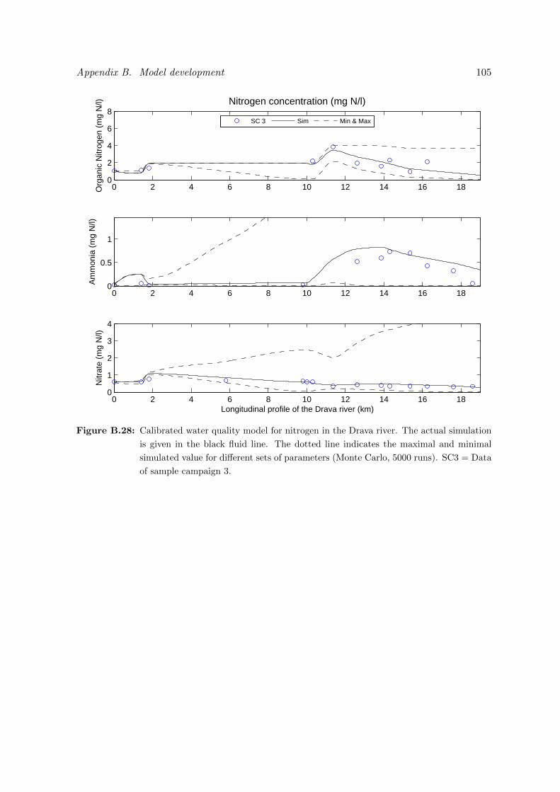
Appendix B. Model development 105
0 2 4 6 8 10 12 14 16 180
2
4
6
8Nitrogen concentration (mg N/l)
Org
anic
Nitr
ogen
(m
g N
/l)
SC 3 Sim Min & Max
0 2 4 6 8 10 12 14 16 180
0.5
1
Am
mon
ia (
mg
N/l)
0 2 4 6 8 10 12 14 16 180
1
2
3
4
Nitr
ate
(mg
N/l)
Longitudinal profile of the Drava river (km)
Figure B.28: Calibrated water quality model for nitrogen in the Drava river. The actual simulation
is given in the black fluid line. The dotted line indicates the maximal and minimal
simulated value for different sets of parameters (Monte Carlo, 5000 runs). SC3 = Data
of sample campaign 3.
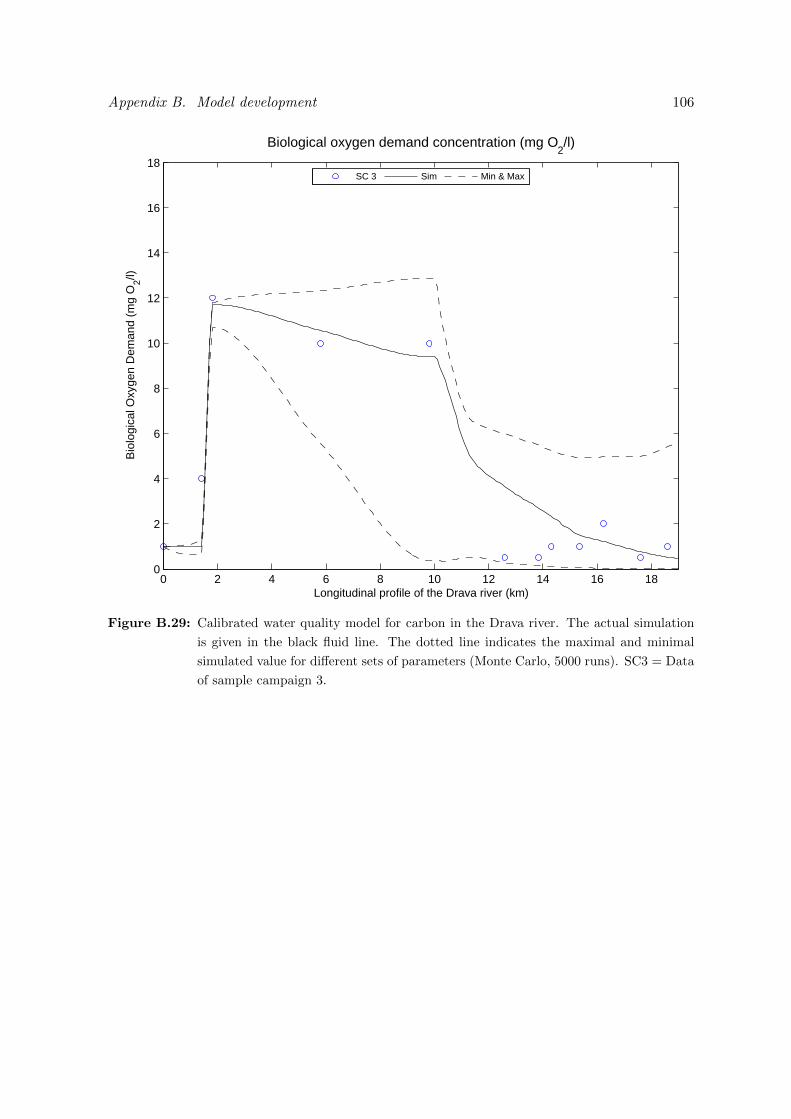
Appendix B. Model development 106
0 2 4 6 8 10 12 14 16 180
2
4
6
8
10
12
14
16
18
Biological oxygen demand concentration (mg O2/l)
Longitudinal profile of the Drava river (km)
Bio
logi
cal O
xyge
n D
eman
d (m
g O
2/l)
SC 3 Sim Min & Max
Figure B.29: Calibrated water quality model for carbon in the Drava river. The actual simulation
is given in the black fluid line. The dotted line indicates the maximal and minimal
simulated value for different sets of parameters (Monte Carlo, 5000 runs). SC3 = Data
of sample campaign 3.
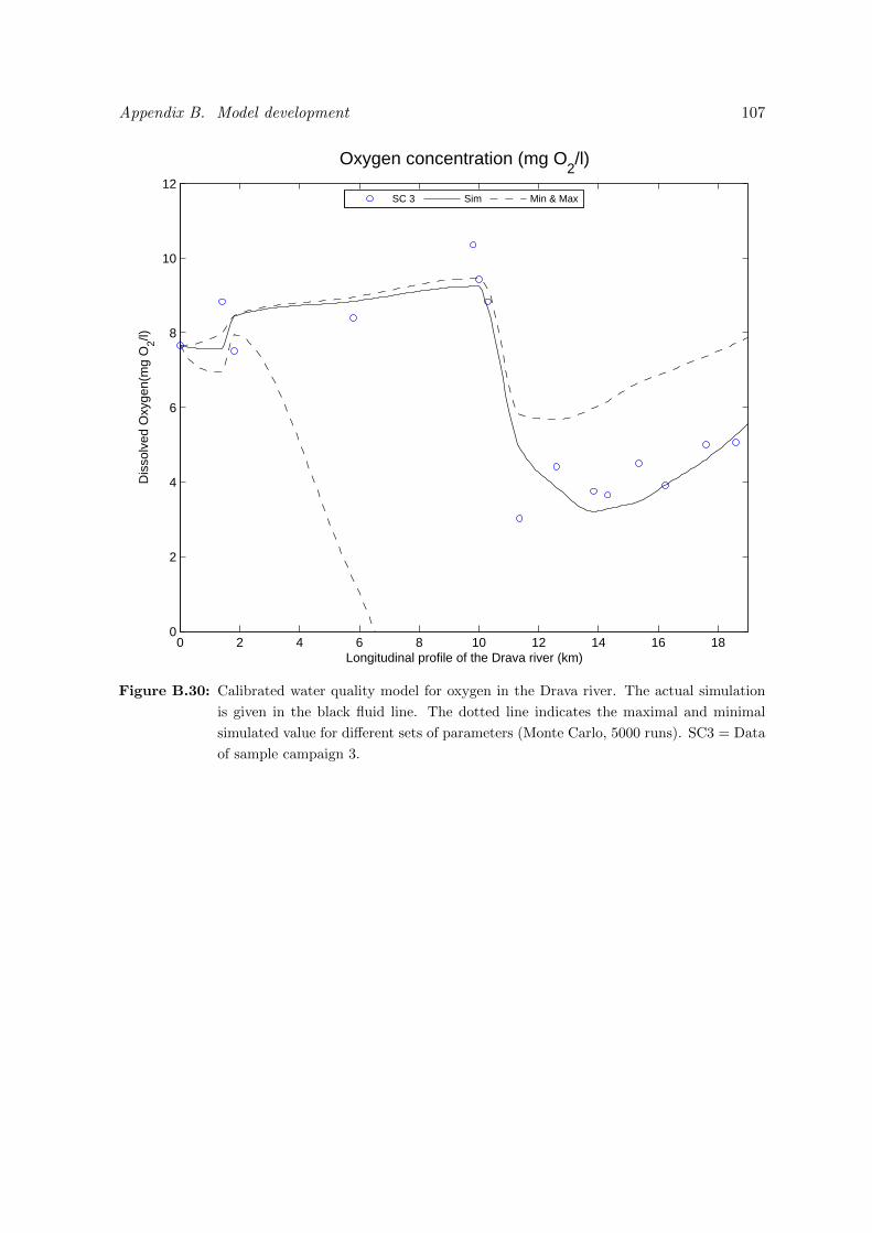
Appendix B. Model development 107
0 2 4 6 8 10 12 14 16 180
2
4
6
8
10
12
Oxygen concentration (mg O2/l)
Longitudinal profile of the Drava river (km)
Dis
solv
ed O
xyge
n(m
g O
2/l)
SC 3 Sim Min & Max
Figure B.30: Calibrated water quality model for oxygen in the Drava river. The actual simulation
is given in the black fluid line. The dotted line indicates the maximal and minimal
simulated value for different sets of parameters (Monte Carlo, 5000 runs). SC3 = Data
of sample campaign 3.
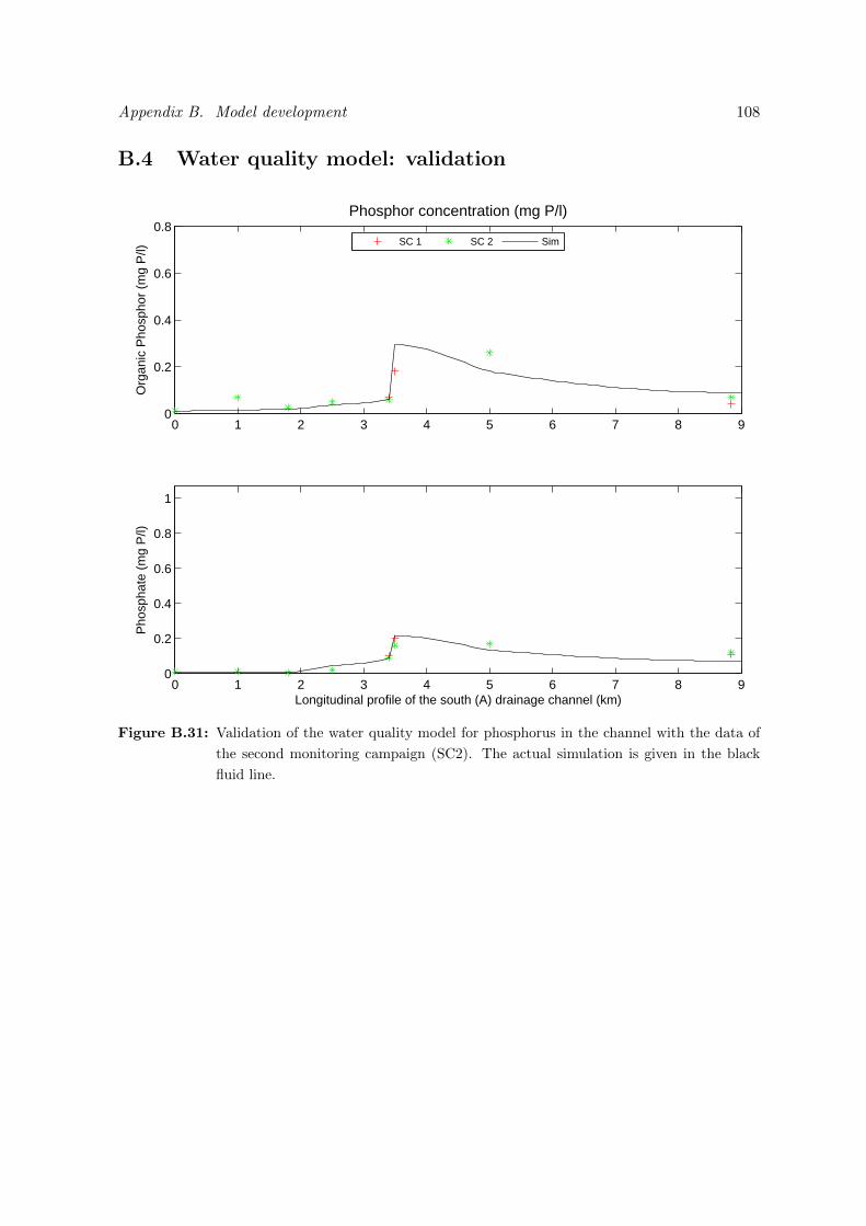
Appendix B. Model development 108
B.4 Water quality model: validation
0 1 2 3 4 5 6 7 8 90
0.2
0.4
0.6
0.8Phosphor concentration (mg P/l)
Org
anic
Pho
spho
r (m
g P
/l)
SC 1 SC 2 Sim
0 1 2 3 4 5 6 7 8 90
0.2
0.4
0.6
0.8
1
Pho
spha
te (
mg
P/l)
Longitudinal profile of the south (A) drainage channel (km)
Figure B.31: Validation of the water quality model for phosphorus in the channel with the data of
the second monitoring campaign (SC2). The actual simulation is given in the black
fluid line.
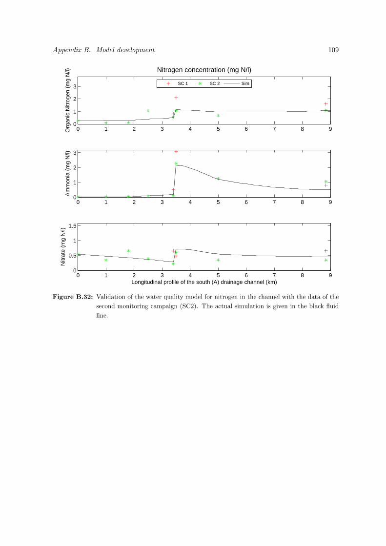
Appendix B. Model development 109
0 1 2 3 4 5 6 7 8 90
1
2
3
Nitrogen concentration (mg N/l)O
rgan
ic N
itrog
en (
mg
N/l)
SC 1 SC 2 Sim
0 1 2 3 4 5 6 7 8 90
1
2
3
Am
mon
ia (
mg
N/l)
0 1 2 3 4 5 6 7 8 90
0.5
1
1.5
Nitr
ate
(mg
N/l)
Longitudinal profile of the south (A) drainage channel (km)
Figure B.32: Validation of the water quality model for nitrogen in the channel with the data of the
second monitoring campaign (SC2). The actual simulation is given in the black fluid
line.
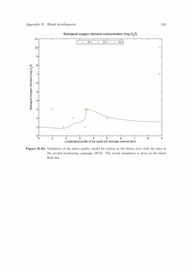
Appendix B. Model development 110
0 1 2 3 4 5 6 7 8 90
1
2
3
4
5
6
7
8
9
10
11
Biological oxygen demand concentration (mg O2/l)
Longitudinal profile of the south (A) drainage channel (km)
Bio
logi
cal O
xyge
n D
eman
d (m
g O
2/l)
SC 1 SC 2 Sim
Figure B.33: Validation of the water quality model for carbon in the Drava river with the data of
the second monitoring campaign (SC2). The actual simulation is given in the black
fluid line.
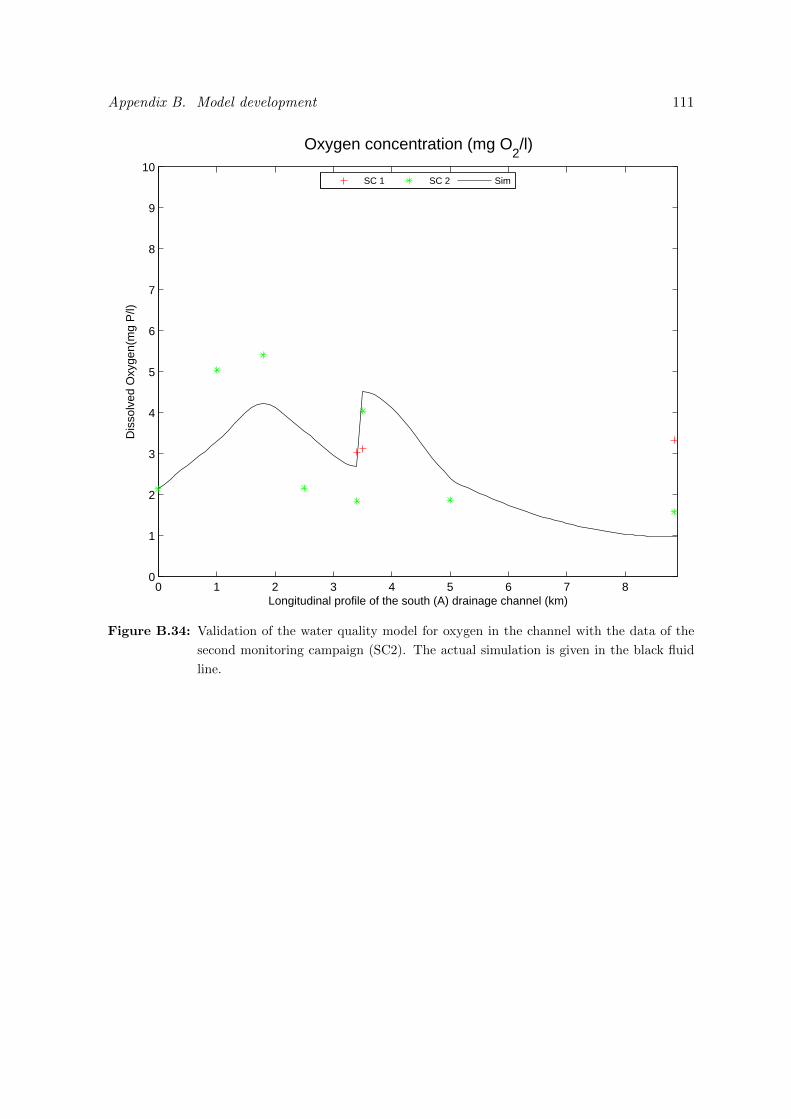
Appendix B. Model development 111
0 1 2 3 4 5 6 7 80
1
2
3
4
5
6
7
8
9
10
Oxygen concentration (mg O2/l)
Longitudinal profile of the south (A) drainage channel (km)
Dis
solv
ed O
xyge
n(m
g P
/l)
SC 1 SC 2 Sim
Figure B.34: Validation of the water quality model for oxygen in the channel with the data of the
second monitoring campaign (SC2). The actual simulation is given in the black fluid
line.
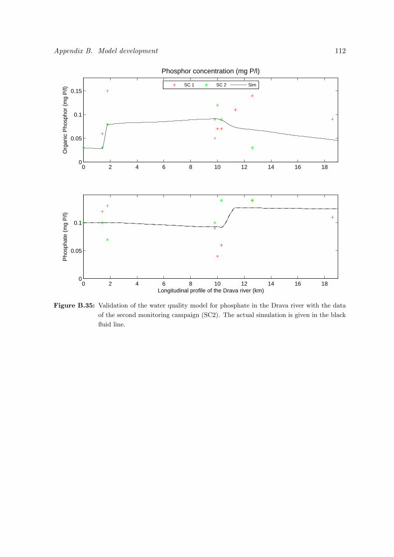
Appendix B. Model development 112
0 2 4 6 8 10 12 14 16 180
0.05
0.1
0.15
Phosphor concentration (mg P/l)O
rgan
ic P
hosp
hor
(mg
P/l)
SC 1 SC 2 Sim
0 2 4 6 8 10 12 14 16 180
0.05
0.1
Pho
spha
te (
mg
P/l)
Longitudinal profile of the Drava river (km)
Figure B.35: Validation of the water quality model for phosphate in the Drava river with the data
of the second monitoring campaign (SC2). The actual simulation is given in the black
fluid line.
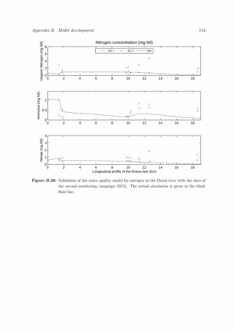
Appendix B. Model development 113
0 2 4 6 8 10 12 14 16 180
2
4
6
8Nitrogen concentration (mg N/l)
Org
anic
Nitr
ogen
(m
g N
/l)
SC 1 SC 2 Sim
0 2 4 6 8 10 12 14 16 180
0.5
1
Am
mon
ia (
mg
N/l)
0 2 4 6 8 10 12 14 16 180
1
2
3
4
Nitr
ate
(mg
N/l)
Longitudinal profile of the Drava river (km)
Figure B.36: Validation of the water quality model for nitrogen in the Drava river with the data of
the second monitoring campaign (SC2). The actual simulation is given in the black
fluid line.
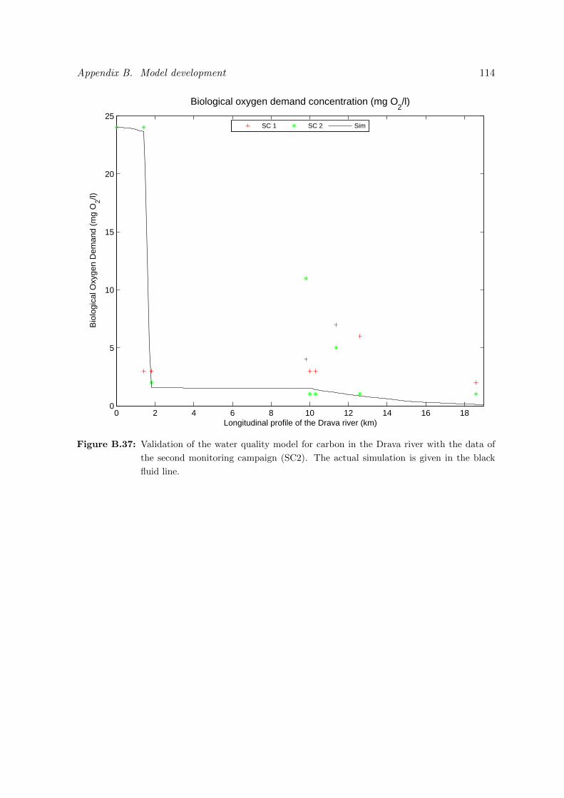
Appendix B. Model development 114
0 2 4 6 8 10 12 14 16 180
5
10
15
20
25
Biological oxygen demand concentration (mg O2/l)
Longitudinal profile of the Drava river (km)
Bio
logi
cal O
xyge
n D
eman
d (m
g O
2/l)
SC 1 SC 2 Sim
Figure B.37: Validation of the water quality model for carbon in the Drava river with the data of
the second monitoring campaign (SC2). The actual simulation is given in the black
fluid line.
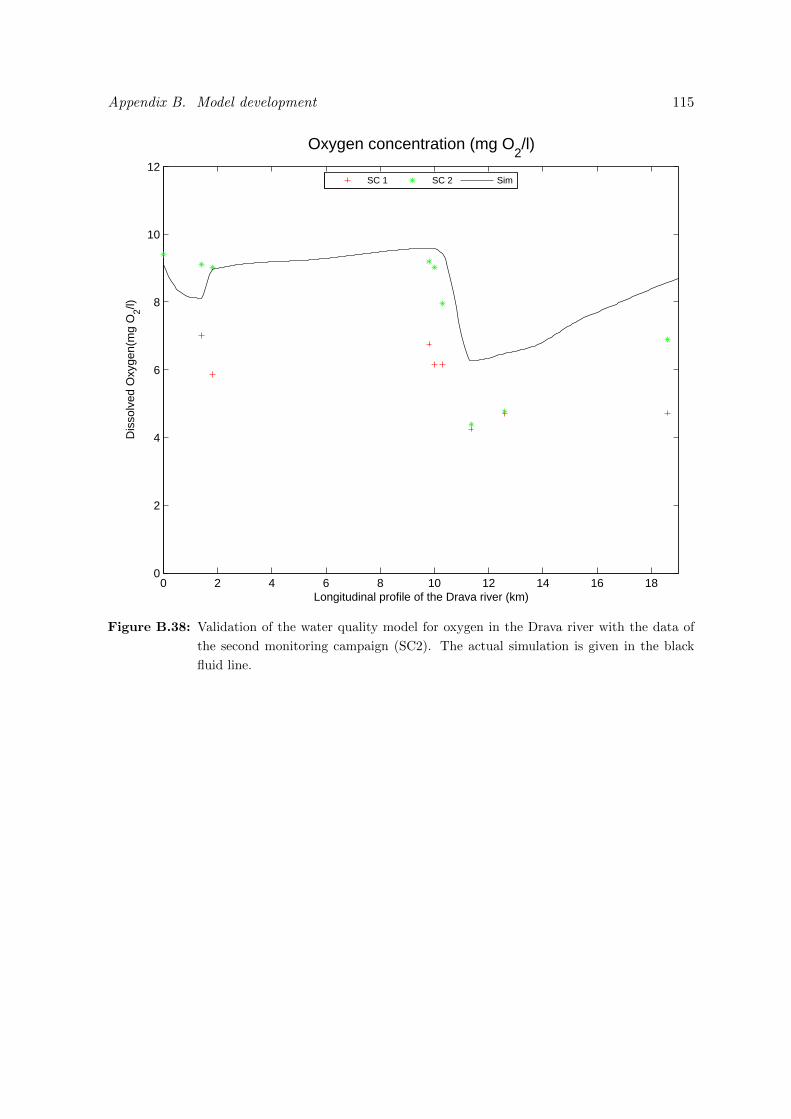
Appendix B. Model development 115
0 2 4 6 8 10 12 14 16 180
2
4
6
8
10
12
Oxygen concentration (mg O2/l)
Longitudinal profile of the Drava river (km)
Dis
solv
ed O
xyge
n(m
g O
2/l)
SC 1 SC 2 Sim
Figure B.38: Validation of the water quality model for oxygen in the Drava river with the data of
the second monitoring campaign (SC2). The actual simulation is given in the black
fluid line.