University of GhentFaculty of Sciences

Department of Mathematical AnalysisClifford Algebra Research Group

Convolutions of hypercomplex Fourier transformswith applications in image processing

Thesis to obtain the academic degree Master of Sciencein Mathematics: Mathematical Physics and Astronomy

By:

K. Rubrecht

Guided by:

prof. dr. ir. H. De Bieprof. dr. ir. A. Pizurica

Academic year:

2013-2014

Preface

When my promoter and I first talked about the subject of this thesis, I was immediatelyconvinced and quietly enthusiastic. The discipline of Clifford algebras is one of those areas inmathematics that has a rich variety in abstraction and also has a lot of applications. Imageprocessing on the other hand is of fundamental importance to our modern day society. Boththese disciplines are still actively evolving. The cross section of these two subjects and thefact that in these domains there is still progress to be made, appealed very much to me asa mathematician and as an engineer. The creation of this work was not an entirely newexperience, as I wrote a thesis to obtain a degree in engineering the year before. It was nocontinuation either, because the subject was entirely different. The fact that there was a lowerthreshold to the subject than in my previous thesis, meant that I could start with the realresearch work early on in the process. As a result this thesis gravitated more towards actualcalculations and research than towards a study of the literature. I hope that the combinedresult of my previous experience and the more research-oriented approach makes this workin a sense more mature. For a mathematician the subject of this thesis is quite applied. Inmy opinion the possibility of applying a formula only adds to the beauty of the formulas inquestion.

Although I had learned from my previous studies, there where still quite a lot of things tolearn and to discover. During the last year I did not only learn a lot on a scientific level,but I also learned a lot on a personal level. This would not have been possible without theguidance of some special people I have to acknowledge. I want to thank my promoter prof.dr. ir. H. De Bie. He introduced me to the subject, carefully corrected the manuscripts andpresentations, answered questions and guided me along the way. I sincerely hope that theresults in this thesis will be of use in his further research on this subject. I would also wantto express my sincere gratitude to my co-promoter prof. dr. ir. A. Pizurica, as a specialist inimage processing, she helped me establish the second part of this thesis. In this second partthe mathematical results of the first part are applied in image processing. Finally I want tothank my family and friends for their enduring and everlasting support.

Disclaimer: The author gives the permission to make this thesis available for consultationand to copy parts of this thesis for personal use. Any other use is subject to the restrictionsof copyright law, one has in particular the obligation to explicitly mention the source whenciting the results in this thesis.

Date:Signature:

1

Contents

I Convolution formulas in Clifford algebras 4

1 Preliminaries and objective 51.1 Clifford algebras and quaternions . . . . . . . . . . . . . . . . . . . . . . . . . . . 5

1.1.1 Clifford algebras . . . . . . . . . . . . . . . . . . . . . . . . . . . . . . 51.1.2 Quaternions . . . . . . . . . . . . . . . . . . . . . . . . . . . . . . . . . 7

1.2 The main objective . . . . . . . . . . . . . . . . . . . . . . . . . . . . . . . . . . . 8

2 Derivation of convolution formulas in the quaternionic case 122.1 The numerical approach . . . . . . . . . . . . . . . . . . . . . . . . . . . . . . . . 122.2 The analytical approach . . . . . . . . . . . . . . . . . . . . . . . . . . . . . . . . 14

2.2.1 Introduction . . . . . . . . . . . . . . . . . . . . . . . . . . . . . . . . 142.2.2 Basic formulas . . . . . . . . . . . . . . . . . . . . . . . . . . . . . . . 16

Commuting and anti-commuting of quaternions . . . . . . . . . . . . . 16Commuting and anti-commuting of quaternions with exponentials . . 18Properties of the quaternionic Fourier transform . . . . . . . . . . . . 19

2.2.3 The case of just one root µ = ν . . . . . . . . . . . . . . . . . . . . . . 202.2.4 The case of anticommuting roots µ, ν . . . . . . . . . . . . . . . . . . 212.2.5 The case of general roots µ, ν . . . . . . . . . . . . . . . . . . . . . . . 25

Derivation of the ‘good’ terms . . . . . . . . . . . . . . . . . . . . . . . 26Derivation of the extra terms . . . . . . . . . . . . . . . . . . . . . . . 28

2.3 Corollary: a quaternionic correlation theorem . . . . . . . . . . . . . . . . . . . . 29

3 Derivation of convolution formulas in the general Clifford algebra case 313.1 The analytical approach . . . . . . . . . . . . . . . . . . . . . . . . . . . . . . . . 31

3.1.1 The case of a single root ik = is . . . . . . . . . . . . . . . . . . . . . . 323.1.2 The case of pairwise anticommuting roots ik . . . . . . . . . . . . . . 33

1. Preparatory steps . . . . . . . . . . . . . . . . . . . . . . . . . . . . 332. Reordering of the exponentials

∏mk=1 e

−ik(zk+yk)uk . . . . . . . . . . 343. Split of the function f . . . . . . . . . . . . . . . . . . . . . . . . . 394. Separating factors in y and z . . . . . . . . . . . . . . . . . . . . . 415. Identification of the geometric Fourier transforms . . . . . . . . . . 446. Further reduction . . . . . . . . . . . . . . . . . . . . . . . . . . . . 457. Verification of the quaternionic case . . . . . . . . . . . . . . . . . . 48

3.1.3 The case of coorthogonal roots . . . . . . . . . . . . . . . . . . . . . . 493.2 Outlook and conclusions . . . . . . . . . . . . . . . . . . . . . . . . . . . . . . . . 52

2

II Applications of quaternionic convolution formulas 54

4 Quaternions in image processing 554.1 Images and color spaces . . . . . . . . . . . . . . . . . . . . . . . . . . . . . . . . 56

4.1.1 The LMS color space . . . . . . . . . . . . . . . . . . . . . . . . . . . . 564.1.2 The RGB color space . . . . . . . . . . . . . . . . . . . . . . . . . . . 564.1.3 Color appearance and other color spaces . . . . . . . . . . . . . . . . . 574.1.4 Images . . . . . . . . . . . . . . . . . . . . . . . . . . . . . . . . . . . . 57

4.2 Quaternionic pixels . . . . . . . . . . . . . . . . . . . . . . . . . . . . . . . . . . . 584.2.1 Quaternions and rotations in color space . . . . . . . . . . . . . . . . . 58

5 Color edge filtering by using quaternions 615.1 The color edge detector in the spatial domain . . . . . . . . . . . . . . . . . . . . 61

5.1.1 Discrete quaternionic convolutions . . . . . . . . . . . . . . . . . . . . 615.1.2 The working principle of the color edge filter . . . . . . . . . . . . . . 64

5.2 The color edge detector in the spectral domain . . . . . . . . . . . . . . . . . . . 665.2.1 The discrete quaternionic Fourier transform . . . . . . . . . . . . . . . 665.2.2 Discretization of the convolution formulas . . . . . . . . . . . . . . . . 685.2.3 Spectrum of the color edge filter . . . . . . . . . . . . . . . . . . . . . 715.2.4 Improvements of the color edge filter . . . . . . . . . . . . . . . . . . . 72

1. A color edge filter without loss of sharpness . . . . . . . . . . . . . 722. Other color edge filters . . . . . . . . . . . . . . . . . . . . . . . . . 76

3

Part I

Convolution formulas in Cliffordalgebras

4

Chapter 1

Preliminaries and objective

The purpose of this small chapter is twofold. In a first section 1.1 we want to provide a quickreview of Clifford algebras and quaternions that can serve as serve as a reference guide to thereader. Readers who are familiar with the concepts of Clifford algebras and quaternions cancertainly skip this section or use it to refresh their memory. Next, we want to explain themain objective of this part of the thesis with the background acquired in the first section.This is done in section 1.2. After reading this chapter the reader should be able to understandthe work of the following chapters.

1.1 Clifford algebras and quaternions

1.1.1 Clifford algebras

Clifford algebras were introduced by the English mathematician William Kingdon Clifford(1845-1879) in 1878. Clifford first named them ‘geometric’ algebras since the importance ofthese algebras comes from successfully uniting the scalar and outer product (informally knowas wedge product) of two vectors into one structure. Doing so leads to geometric entities of acertain grade k with a k-dimensional extent beyond scalars (grade 0) and vectors (grade 1).Therefore a Clifford algebra is a graded algebra and its entities are in general called multi-vectors, with notable examples the oriented surface and oriented volume respectively calledthe bivector (grade 2) and trivector (grade 3). Clifford algebras were rediscovered in othersettings. Perhaps the most famous example is the factorization of the Klein-Gordon equationin 1928. The gamma matrices in the Dirac equation are in fact the generators of the Clif-ford algebra Cl1,3 with the Lorentz signature. Similar factorizations led to the discipline thatis now known as Clifford analysis. A very important special case of Clifford algebras is thenon-commutative algebra of the quaternions H. These quaternions were already discovered in1843 when according to the famous anecdote William Rowan Hamilton(1805-1865) engravedtheir basic relations on Brougham Bridge in Dublin. The important link between Cliffordalgebras and the orthogonal groups makes them useful for an alternative description of or-thogonal transformations. Rotations in 3-dimensional space are most efficiently and easilyimplemented using quaternions in graphical software. For a nice basic introduction to Cliffordalgebras and Clifford analysis the reader can consult [10]. For a detailed exposition from the

5

geometric point of view, including geometric interpretations and applications in computervision, we refer the reader to [12]. Let us start by immediately defining the Clifford algebras.

Definition 1 The real Clifford algebra Cl0,m over Rm is the algebra generated by ei, i =1, . . . ,m, under the relations

eiej + ejei = 0, i 6= j (1.1)

e2i = −1.

The noncommutative product on the algebra (by linearity and the basic relations) is called thegeometric product, and is denoted without a symbol. The Clifford algebras have dimension2m as a vector space over R. They can be decomposed as Cl0,m = ⊕mk=0Clk0,m with Clk0,m thespace of blades of grade k defined by

Clk0,m := span{ei1 . . . eik , i1 < . . . < ik}.

One sees that the vector space Rm can be incorporated in the Clifford algebra as the com-ponent Cl10,m. A basis transformation of this component determines the change in the other

components. Usually these vectors x :=∑m

j=1 xjej ∈ Cl10,m are underlined, but here we willuse the convention that the vectors x will not be underlined when they are used as variables.

Next we define the inner product and the wedge product of two vectors x and y as

〈x, y〉 := −m∑j=1

xjyj

x ∧ y :=∑j<k

ejek(xjyk − xkyj).

If 〈x, y〉 = 0 then we call the vectors x and y orthogonal, when x ∧ y = 0 they are colinear.We can capture both in the term ‘coorthogonal’ of which the more general definition will begiven later on.

For m = 3 this wedge product corresponds to the vector product. With the basic relationsone can easily verify that one has:

〈x, y〉 = −xy + yx

2

x ∧ y =xy − yx

2xy = x ∧ y − 〈x, y〉.

A special case of multivectors are the so-called blades. These can be defined by two equivalentdefinitions.

6

Definition 2 A k-blade A is a multivector of grade k which can be written as an outerproduct of vectors a1, . . . , ak ∈ Cl10,m or as a geometric product of mutually orthogonal vectors

b1, . . . , bk ∈ Cl10,m, bi ⊥ bj(i 6= j).

A = a1 ∧ . . . ∧ ak = b1 b2 . . . bk

The fact that these definitions are equivalent follows simply from the fact that one can subtract

the projection on the orthogonal component in the wedge product a1∧a2 = a1∧a2−〈a1,a2〉〈a1,a1〉a1.

This is in fact nothing more than a disguised Gramm-Schmidt procedure. By convention wewill denote blades with an uppercase latin letter, arbitrary Clifford numbers will be denotedwith lowercase latin letters.

In this master thesis, we will always consider functions f taking values in Cl0,m, unless ex-plicitly mentioned. Such functions can be decomposed as a sum of so-called basis blades.

f = f0 +m∑i=1

eifi +∑i<j

eiejfij + . . .+ e1 . . . emf1...m

with f0, fi, fij , . . . , f1...m all real- or complex-valued functions on Rm.

1.1.2 Quaternions

A special Clifford algebra is the algebra of the quaternions H.

Definition 3 The quaternion algebra H is the algebra over R generated by the basic ele-ments i, j, k, under the relations

i2 = j2 = k2 = ijk = −1. (1.2)

These basic relations immediately imply:

ij = −ji = k

jk = −kj = i

ki = −ik = j.

The quaternions H are isomorphic to the Clifford algebra Cl0,2 by the following isomorphism:

φ1 : Cl0,2 7→ H, e1 7→ i e2 7→ j e1e2 7→ k.

7

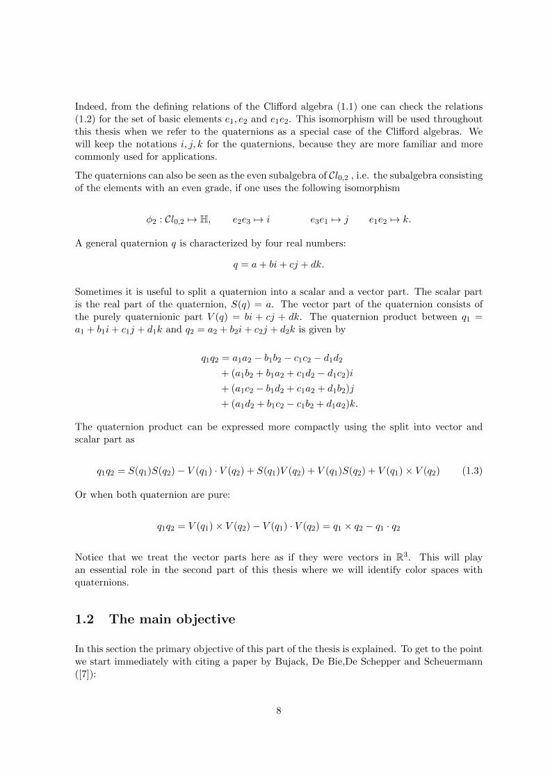
Indeed, from the defining relations of the Clifford algebra (1.1) one can check the relations(1.2) for the set of basic elements e1, e2 and e1e2. This isomorphism will be used throughoutthis thesis when we refer to the quaternions as a special case of the Clifford algebras. Wewill keep the notations i, j, k for the quaternions, because they are more familiar and morecommonly used for applications.

The quaternions can also be seen as the even subalgebra of Cl0,2 , i.e. the subalgebra consistingof the elements with an even grade, if one uses the following isomorphism

φ2 : Cl0,2 7→ H, e2e3 7→ i e3e1 7→ j e1e2 7→ k.

A general quaternion q is characterized by four real numbers:

q = a+ bi+ cj + dk.

Sometimes it is useful to split a quaternion into a scalar and a vector part. The scalar partis the real part of the quaternion, S(q) = a. The vector part of the quaternion consists ofthe purely quaternionic part V (q) = bi + cj + dk. The quaternion product between q1 =a1 + b1i+ c1j + d1k and q2 = a2 + b2i+ c2j + d2k is given by

q1q2 = a1a2 − b1b2 − c1c2 − d1d2+ (a1b2 + b1a2 + c1d2 − d1c2)i+ (a1c2 − b1d2 + c1a2 + d1b2)j

+ (a1d2 + b1c2 − c1b2 + d1a2)k.

The quaternion product can be expressed more compactly using the split into vector andscalar part as

q1q2 = S(q1)S(q2)− V (q1) · V (q2) + S(q1)V (q2) + V (q1)S(q2) + V (q1)× V (q2) (1.3)

Or when both quaternion are pure:

q1q2 = V (q1)× V (q2)− V (q1) · V (q2) = q1 × q2 − q1 · q2

Notice that we treat the vector parts here as if they were vectors in R3. This will playan essential role in the second part of this thesis where we will identify color spaces withquaternions.

1.2 The main objective

In this section the primary objective of this part of the thesis is explained. To get to the pointwe start immediately with citing a paper by Bujack, De Bie,De Schepper and Scheuermann([7]):

8

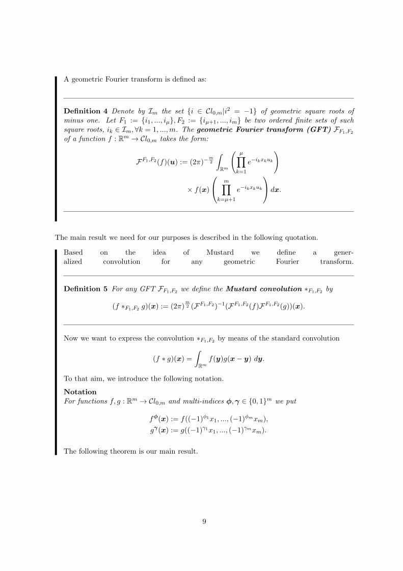
A geometric Fourier transform is defined as:

Definition 4 Denote by Im the set {i ∈ Cl0,m|i2 = −1} of geometric square roots ofminus one. Let F1 := {i1, ..., iµ}, F2 := {iµ+1, ..., im} be two ordered finite sets of suchsquare roots, ik ∈ Im,∀k = 1, ...,m. The geometric Fourier transform (GFT) FF1,F2

of a function f : Rm → Cl0,m takes the form:

FF1,F2(f)(u) := (2π)−m2

∫Rm

(µ∏k=1

e−ikxkuk

)

× f(x)

m∏k=µ+1

e−ikxkuk

dx.

The main result we need for our purposes is described in the following quotation.

Based on the idea of Mustard we define a gener-alized convolution for any geometric Fourier transform.

Definition 5 For any GFT FF1,F2 we define the Mustard convolution ∗F1,F2 by

(f ∗F1,F2 g)(x) := (2π)m2 (FF1,F2)−1(FF1,F2(f)FF1,F2(g))(x).

Now we want to express the convolution ∗F1,F2 by means of the standard convolution

(f ∗ g)(x) =

∫Rm

f(y)g(x− y) dy.

To that aim, we introduce the following notation.

NotationFor functions f, g : Rm → Cl0,m and multi-indices φ,γ ∈ {0, 1}m we put

fφ(x) := f((−1)φ1x1, ..., (−1)φmxm),

gγ(x) := g((−1)γ1x1, ..., (−1)γmxm).

The following theorem is our main result.

9

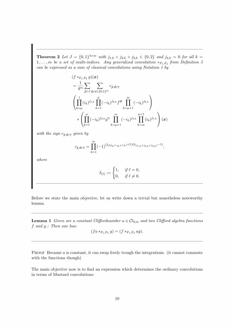
Theorem 2 Let J = {0, 1}4×m with j1,k + j2,k + j3,k ∈ {0, 2} and j4,k = 0 for all k =1, . . . ,m be a set of multi-indices. Any generalized convolution ∗F1,F2 from Definition 5can be expressed as a sum of classical convolutions using Notation 1 by

(f ∗F1,F2 g)(x)

=1

4m

∑j∈J

∑φ,γ∈{0,1}m

cj,φ,γ 1∏k=µ

(ik)j1,k

µ∏k=1

(−ik)j2,kfφm∏

k=µ+1

(−ik)j2,k

∗

µ∏k=1

(−ik)j3,kgγm∏

k=µ+1

(−ik)j3,kµ+1∏k=m

(ik)j1,k

(x)

with the sign cj,φ,γ given by

cj,φ,γ =

m∏k=1

(−1)(j(2φk+γk+1,k)+1)(δ(j1,k+j2,k+j3,k)−1),

where

δ(`) :=

{1, if ` = 0,

0, if ` 6= 0.

Before we state the main objective, let us write down a trivial but nonetheless noteworthylemma.

Lemma 1 Given are a constant Cliffordnumber a ∈ Cl0,m and two Clifford algebra functionsf and g.: Then one has:

(fa ∗F1,F2 g) = (f ∗F1,F2 ag).

Proof Because a is constant, it can swap freely trough the integrations. (it cannot commutewith the functions though)

The main objective now is to find an expression which determines the ordinary convolutionsin terms of Mustard convolutions:

10

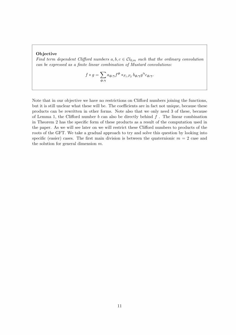
ObjectiveFind term dependent Clifford numbers a, b, c ∈ Cl0,m such that the ordinary convolutioncan be expressed as a finite linear combination of Mustard convolutions:

f ∗ g =∑φ,γ

aφ,γfφ ∗F1,F2 bφ,γg

γcφ,γ .

Note that in our objective we have no restrictions on Clifford numbers joining the functions,but it is still unclear what these will be. The coefficients are in fact not unique, because theseproducts can be rewritten in other forms. Note also that we only need 3 of these, becauseof Lemma 1, the Clifford number b can also be directly behind f . The linear combinationin Theorem 2 has the specific form of these products as a result of the computation used inthe paper. As we will see later on we will restrict these Clifford numbers to products of theroots of the GFT. We take a gradual approach to try and solve this question by looking intospecific (easier) cases. The first main division is between the quaternionic m = 2 case andthe solution for general dimension m.

11

Chapter 2

Derivation of convolution formulasin the quaternionic case

With an outlook on applications we first consider the special case of quaternions (wherem = 2), and in particular the case where the exponentials are on the left side of the functions.

Definition 6 Denote by µ, ν ∈ I2 two geometric square roots of minus one, i.e. µ2 =ν2 = −1. The left quaternionic Fourier transform (left qFT) Fµ,ν of a functionf : R2 → Cl0,2 ∼= H is defined as:

Fµ,ν(f)(y) =1

2π

∫R2

e−µx1y1e−νx2y2f(x)dx (2.1)

There exist a lot of different Fourier transforms in Clifford analysis, and the above definition isobviously not unique. Due to the non commutative character of the quaternions the transformcan also be defined by sandwiching the function f with two exponentials, or by putting theexponentials on the right side. These are not the only 3 options, for an overview of differentquaternionic Fourier transforms (qFTs) and their basic properties the reader can for exampleconsult [6] or [17]. For some material on Fourier transforms in the general Clifford algebrasetting one could opt for one of the papers ([8],[9],[5]). Let us suppose for this chapter thatwe are working with transform (2.1) where µ and ν denote linear independent square rootsof -1.

2.1 The numerical approach

It is clear that in Cl0,2 every element can be spanned by {1, µ, ν, µν}. Observing Theorem 2we find that in our case it reduces to:

12

(f ∗µ,ν g)(x)

=1

16

∑j∈J

∑φ,γ∈{0,1}2

cj,φ,γ(ν)j1,2(µ)j1,1(−µ)j2,1(−ν)j2,2fφ ∗ (−µ)j3,1(−ν)j3,2gγ(x) (2.2)

where we denoted f ∗{µ,ν},{∅} g(x) shortly as f ∗µ,ν g(x) for now.

With the above considerations we can expect that every factor of the form (ν)j1,2(µ)j1,1(−µ)j2,1(−ν)j2,2

reduces to a sum in the span of {1, µ, ν, µν} with coefficients dependent on J . Every termwill as a consequence be of the form c(αfφ ∗ βgγ) with α, β ∈ {1, µ, ν, µν} (for brevity it willsometimes simply be denoted as α|β ).

Given that there are 16 combinations for α, β and another 16 for φ, γ, we see that it canbe expressed in at most 256 terms. With (2.2) we can now also compute every Mustardconvolution of the form (αfφ ∗µ,ν βgγ). For similar reasons they will also be a combinationof the 256 ordinary convolution terms. This gives us a scheme for calculating the coefficientsin the reverse formula:

• Rewrite (f ∗µ,ν g) in terms of (αfφ ∗ βgγ)

• Do the same for all the other convolutions of the form: (αfφ ∗µ,ν βgγ)

• Solve the system with the matrix of coefficients obtained by the 256 × 256 coefficientsand the constant vector [1, 0, . . . , 0]T (just constant one for the ordinary convolutionterm ((f ∗ g)(x))

• This results in the coefficients for the ordinary convolution (f ∗g)(x) expressed in termsof the Mustard convolution.

It is here already noteworthy that the factors of the form (ν)j1,2(µ)j1,1(−µ)j2,1(−ν)j2,2 reducemuch more easily when we suppose anticommutation of µ and ν. This led to a subdivision inthree cases for the analytical approach later on:

1. there is just one root µ = ν

2. the roots µ and ν are anticommuting

3. the roots µ and ν are general linearly independent roots.

The above procedure was numerically implemented using MatLab and resulted in the followingformulas for the anticommuting (second) case:

Mustard convolution expressed in terms of the ordinary convolution:

(f ∗µ,ν g) =1

4[f ∗ g + f ∗ g(0,1) + f ∗ g(1,0) + f ∗ g(1,1)

− νf ∗ νg + νf ∗ νg(0,1) − νf ∗ νg(1,0) + νf ∗ νg(1,1)

− µf (0,1) ∗ µg − µf (0,1) ∗ µg(0,1) + µf (0,1) ∗ µg(1,0) + µf (0,1) ∗ µg(1,1)

− νµf (0,1) ∗ νµg + νµf (0,1) ∗ νµg(0,1) + νµf (0,1) ∗ νµg(1,0) − νµf (0,1) ∗ νµg(1,1)]

13

Ordinary convolution expressed in terms of the Mustard convolution:

(f ∗ g) =1

4[f ∗µ,ν g + f ∗µ,ν g(0,1) + f ∗µ,ν g(1,0) + f ∗µ,ν g(1,1)

− νf ∗µ,ν νg + νf ∗µ,ν νg(0,1) − νf ∗µ,ν νg(1,0) + νf ∗µ,ν νg(1,1)

− µf (0,1) ∗µ,ν µg − µf (0,1) ∗µ,ν µg(0,1) + µf (0,1) ∗µ,ν µg(1,0) + µf (0,1) ∗µ,ν µg(1,1)

− νµf (0,1) ∗µ,ν νµg + νµf (0,1) ∗µ,ν νµg(0,1) + νµf (0,1) ∗µ,ν νµg(1,0) − νµf (0,1) ∗µ,ν νµg(1,1)](2.3)

It is remarkable that the formulas have exactly the same coefficients. The general quaternioniccase breaks this symmetry and gives rise to extra terms of the form 1|1, µν|1 and 1|µν infunction of the anticommutator a = {µ, ν} and a2. This was numerically observed by usinga small value for a.

Although these computations allow us already some basic insights, such as the fact thatanticommutativity was necessary to obtain the same coefficients in both directions, we needan analytical approach to explain this.

2.2 The analytical approach

2.2.1 Introduction

The paper [8] by Bujack, Scheuermann and Hitzer establishes a technical theorem that calcu-lates the interaction of the ordinary convolution with a very broad class of geometric Fouriertransforms. The results are technical and need a lot of lemmas, but the theorem itself is basi-cally a rework of the classical proof of the convolution theorem. The big difference is that thelack of commutation gives rise to extra terms, because one has to commute the exponentialsto separate those belonging to f and g in (f ∗ g). Luckily this can be done by the use ofsplits in commuting (q−) and anticommuting (q+) parts. It works with generalizations of thefollowing formula:

q = q+ + q−

q± =1

2(q ± µqµ)

q±ecµ = e∓cµq± c ∈ R

This split of quaternions is often used, some background and a more detailed explanation canbe found in [13]. Although we will follow our own approach, the following (adapted) theoremis the main result of [8] :

14

Theorem 3 Let a, b, c be Cliffordfunctions with a(x) = (c∗b)(x) and F1, F2 be coorthogo-nal, seperable and linear with respect to the first argument, j, j′ ∈ {0, 1}µ,k,k′ ∈ {0, 1}ν−µand J ∈ {0, 1}µ×µ and K ∈ {0, 1}(ν−µ)×(ν−µ) are the strictly lower, respectively upper, tri-angular matrices with rows (J)l, (K)l−µ summing up to (

∑µl=1(J)l) mod 2 = j respectively

(∑ν

l=µ+1(K)l−µ) mod 2 = k, then the geometric Fourier transform of A satisfies:

FF1,F2(a)(u) =∑

j,j′,k,k′

∑J,K

(FF1(j),F2(k+k′)(c)(u))cj′ (F1)F(F1(j′))cJ ,(F2)cK

(bck′ (F2))(u)

Theorem 3 is very useful for our purpose, because it is practically equivalent to what we arelooking for. Indeed, one has to note that after applying the inverse transform to both sides,and using linearity, we can use this theorem to obtain what we want by rearranging the termson the right hand side to express them as Mustard convolutions. Although this would be apossible approach, there are several major drawbacks. The first transform in the equationis a so called Geometric Trigonometric Transform (GTT). To have Mustard convolutionsthis transform would have to be rewritten as a sum of Geometric Fourier Transforms. Thecommuting and anticommuting parts are denoted with the ck subscripts and are not explicitlydetermined. The summation over the matrices J and K are not really handy, and last butnot least the theorem supposes that the square roots of −1 in the Fourier Transform are‘coorthogonal’ blades.

Definition 7 Two blades A,B ∈ Cl0,m are defined to be coorthogonal when swapping themonly causes a sign change:

AB = ±BA

In the same paper [8] where the theorem is proven, they prove that coorthogonality impliesthat A and B can be written as real multiples of certain basis blades with respect to a certainbasis of the Clifford algebra. The coorthogonality can thus be interpreted as the coorthogo-nality of their generating vectors, which in turn justifies the use of this terminology. In thismaster thesis we will also allow this definition of coorthogonality for arbitrary multivectors,where the name is in fact misleading. In the simple case of quaternions the coorthogonalityreduces to either commutativity or anticommutativity of µ and ν. Two commuting purequaternions are linearly dependent, so only anticommutativity is non-trivial.

We will give alternative versions of Theorem 3 which incorporate other cases, but do notmake use of the most general geometric Fourier transform. In this work the roots will not berestricted to blades. For the quaternions we will even derive the most general case where theroots are not coorthogonal. To gain more insight we opted to start our derivation from the

15

simpler case of the quaternions to work our way up to general Clifford algebras, in this way weget to manageable formulas without any redundant terms. This will establish a proof for thenumerically obtained formula (2.3). Before accomplishing the derivation of the quaternionicconvolution formulas we introduce some basic formulas and techniques.

2.2.2 Basic formulas

In this section we summarize some of the basic formulas that are going to be used to derivethe expressions later on. They form the basic toolbox for dealing with these problems. Wetook as a starting point the good reference work of Hitzer and Sangwine ([14]). Denote byIm the set {i ∈ Cl0,m|i2 = −1} of geometric square roots of minus one. In the basic formulasµ, ν denote elements of I2 ∼= H and q, r denote elements of Cl0,2 .

Commuting and anti-commuting of quaternions

We define the commuting (j = 0) and the anticommuting (j = 1) part of a quaternion q withrespect to a quaternion r as:

q = qc0(r) + qc1(r)

qcj(r) =1

2(q + (−1)jr−1qr)

qc0(r)r = rqc0(r)

qc1(r)r = −rqc1(r).

(2.4)

This definition uses a notation which complies with a more general definition given in [8]. Inthe case we take the commuting or part with respect to µ a square root of −1, we can keepin mind that µ−1 = −µ. Then the formulas are rewritten as:

q = qc0(µ) + qc1(µ) = q− + q+

qcj(µ) = q∓ =1

2(q − (−1)jµqµ)

q−µ = µq−

q+µ = −µq+.

Here we introduced the notations qc0(µ) = q− and qc1(µ) = q+. These shorter notations aresometimes used when the quaternion we wish to commute is clear from the context. Ingeneral we will avoid this notation because the fact that q− is the commuting part may causeconfusion.

Now suppose we are dealing with two square roots of −1, µ and ν. We introduce the anti-commutator:

a = {µ, ν} = µν + νµ ∈ R

16

The anticommutator is always in R in the quaternionic case. When µ and ν are square roots of−1 they are purely quaternionic and simple calculations reveal that they satisfy the followingconditions:

µ = b1i+ c1j + d1k b21 + c21 + d21 = 1

ν = b2i+ c2j + d2k b22 + c22 + d22 = 1

a = {µ, ν} = µν + νµ

= −b1b2 − c1c2 − d1d2,

where i, j, k are the standard quaternionic units.

We can make use of the fact that a is in R to simplify a lot of calculations. The (anti)commutingparts of µ with respect to ν are for example:

µc0(ν) = µ− =1

2(µ− νµν) = −a

2ν

µc1(ν) = µ+ =1

2(µ+ νµν) = µ+

a

2ν

These commuting parts have interesting properties:

µ2 = µ2+ + µ2− = −1 (2.5)

µ+µ− + µ−µ+ = 0. (2.6)

These can be derived by evaluating µ2ν in two different ways. We have

−ν = µ2ν

= (µ+ + µ−)2ν

= (µ2+ + µ+µ− + µ−µ+ + µ2−)ν

= ν(µ2+ − µ+µ− − µ−µ+ + µ2−),

but we have also

−ν = νµ2

= ν(µ+ + µ−)2

= ν(µ2+ + µ+µ− + µ−µ+ + µ2−)

which leads to (2.5) and (2.6) by equating the two derivations:

ν(µ2+ − µ+µ− − µ−µ+ + µ2−) = ν(µ2+ + µ+µ− + µ−µ+ + µ2−)

17

Commuting and anti-commuting of quaternions with exponentials

In the qFT we have occurrences of quaternionic exponential functions (defined by their seriesexpression), which are based on square roots of −1. So we have eµθ = cos θ+ µ sin θ. We canderive the following commutation relations for such functions.

q = q+ + q− = qc0(µ) + qc1(µ)

q±eθµ = e∓θµq± θ ∈ R.

(2.7)

We will also frequently use its commuting and anticommuting parts:

e−νθcj(µ)

=1

2(e−νθ − (−1)jµ(cos (θ)− ν sin (θ))µ)

=1

2(e−νθ + (−1)jeνθ + a(−1)jµ sin (θ))

=1

2(e−νθ + (−1)jeνθ +

a

2(−1)jeµθ − a

2(−1)je−µθ)

(2.8)

For this case a = 0, which we will encounter later on, the formulas reduce to:

e−νθcj(µ)

=1

2(e−νθ − (−1)jµe−νθµ)

=1

2(e−νθ − (−1)jµ(cos (θ)− ν sin (θ))µ)

=1

2(e−νθ + (−1)jeνθ)

=

{cos θ, if j = 0,

−ν sin θ, if j = 1.

In this case the commuting part is the cosine, while the anticommuting part is the part withthe sine. One could have expected this on the basis of eµθ = cos θ + µ sin θ and the fact µanticommutes with ν in this case.

We can apply this with the purpose of swapping an element of I2 and an exponential.

µe−νθ = (µ+ + µ−)e−νθ

= eνθµ+ + e−νθµ−

= [eνθ(µ+a

2ν)− e−νθ a

2ν].

(2.9)

Later on we will also need the swapping of two elements of I2 and their exponentials.

18

νµe−µθe−νθ = [eµθν+ + e−µθν−][eνθµ+ + e−νθµ−]

= eµθeνθ[(ν+)c0νµ+ + (ν+)c1νµ−]

+ e−µθeνθ[(ν−)c0νµ+ + (ν−)c1νµ−]

+ eµθe−νθ[(ν+)c1νµ+ + (ν+)c0νµ−]

+ e−µθe−νθ[(ν−)c1νµ+ + (ν−)c0νµ−].

Notice that in this case the plus/minus-notation (µ+)+ would have been ambiguous. Easycalculations yield the following:

(ν+)c0ν =a

2µ+

(ν+)c1ν = ν +a

2µ−

(ν−)c0ν = −a2µ+

(ν−)c1ν = −a2µ−.

(2.10)

Making use of these calculations (2.10), and the property (2.6), we can eventually simplifythe expressions behind the exponentials.

νµe−µθe−νθ = eµθeνθ[νµ+] + e−µθe−νθ[a

2]

= eµθeνθ[νµ− a

2] + e−µθe−νθ[

a

2].

(2.11)

Properties of the quaternionic Fourier transform

We can translate the calculations on the exponentials to properties of the quaternionic Fouriertransform (qFT) (defined in definition 6) An easy to prove, but very important property isthe change of signs of the roots.

F (−1)φ1µ,(−1)φ2 ν(g)(u) =

1

2π

∫R2

e−(−1)φ1µx1u1e−(−1)

φ2 νx2u2g(x)dx

= Fµ,ν(gφ)(u).

(2.12)

It is obtained by performing a substitution in the integral (x→ xφ).

In the case of µ and ν are anticommuting it is also easy to obtain that passing µ and/or νthrough the transform changes just the sign of the corresponding exponential and thus of thearguments.

µkνlFµ,ν(g)(u) =1

2πµkνl

∫R2

e−µx1u1e−νx2u2g(x)dx

=1

2π

∫R2

e−(−1)lµx1u1e−(−1)

kνx2u2µkνlg(x)dx

= Fµ,ν(µkνlgl,k)(u)

(2.13)

19

In the case where {µ, ν} = a, we can derive the extended property making use of equations(2.9) and (2.11). This yields after some computations:

µFµ,ν(g)(u) = Fµ,ν(µg(0,1))(u) +a

2Fµ,ν(νg(0,1))− a

2Fµ,ν(νg(0,0))

νFµ,ν(g)(u) = Fµ,ν(νg(1,0))(u) +a

2Fµ,ν(µg(1,0))− a

2Fµ,ν(µg(0,0))

νµFµ,ν(g)(u) = Fµ,ν(νµg(1,1))(u)− a

2Fµ,ν(g(1,1))(u) +

a

2Fµ,ν(g(0,0))(u)

µνFµ,ν(g)(u) = Fµ,ν(µνg(1,1))(u)− a

2Fµ,ν(g(1,1))(u) +

a

2Fµ,ν(g(0,0))(u).

(2.14)

2.2.3 The case of just one root µ = ν

When we have just one root the transform reduces to:

Fµ(f)(y) =1

2π

∫R2

e−µ(x1y1+x2y2)f(x)dx.

Now we can compute the interaction by applying the definitions and subsequently taking theintegrals to the outside (as an application of Fubini’s theorem):

Fµ(f ∗ g(x))(u) =1

2π

∫R2

e−µ(x1u1+x2u2)(f ∗ g)(x)dx

=1

2π

∫R2

e−µ(x1u1+x2u2)∫R2

f(x− y)g(y)dydx

=1

2π

∫R2

∫R2

e−µ(x1u1+x2u2)f(x− y)g(y)dydx

=1

2π

∫R2

∫R2

e−µ[(z1+y1)u1+(z2+y2)u2]f(z)g(y)dzdy

=1

2π

∫R2

∫R2

e−µ(z1u1+z2u2)e−µ(y1u1+y2u2)f(z)g(y)dzdy

In the last step we have made the substitution x→ z+ y. Because there is just one root, allthe exponential functions commute, and the exponential property holds. This will no longerbe the case later on. We can continue by separating the parts in z and the parts in y.

20

Fµ(f ∗ g(x))(u)

=1

2π

∫R2

∫R2

e−µ(z1u1+z2u2)[f(z)c0(µ)e−µ(y1u1+y2u2) + f(z)c1(µ)e

µ(y1u1+y2u2)]g(y)dzdy

=1

2

1

2π

∫R2

∫R2

e−µ(z1u1+z2u2)[(f(z)− µf(z)µ)e−µ(y1u1+y2u2) + (f(z) + µf(z)µ)eµ(y1u1+y2u2)]g(y)dzdy

=1

2

1

2π

∫R2

∫R2

e−µ(z1u1+z2u2)f(z)e−µ(y1u1+y2u2)g(y)− e−µ(z1u1+z2u2)µf(z)e−µ(y1u1+y2u2)µg(y)

+ (e−µ(z1u1+z2u2)f(z)eµ(y1u1+y2u2)g(y) + e−µ(z1u1+z2u2)µf(z)eµ(y1u1+y2u2)µg(y)dzdy

=2π

2[Fµ(f)(u)Fµ(g)(u)−Fµ(µf)(u)Fµ(µg)(u) + Fµ(f)(u)Fµ(g(1,1))(u) + Fµ(µf)(u)Fµ(µg(1,1))(u).

In a final step we apply the inverse Fourier transform to both sides, by using the definitionof the Mustard convolution 5 we get

f ∗ g(x) =1

2[f ∗µ g − µf ∗µ µg + f ∗µ g(1,1) + µf ∗µ µg(1,1)].

This gives us a first and easy result. Although it is a quite simple calculation it alreadyshowcases some of the frequently occurring and important steps that will be made later on.We summarize our result in the theorem below.

Theorem 4 Let f and g be quaternionic functions on R2, and Fµ the left qFT with one rootµ. The ordinary convolution can then be expressed as a sum of Mustard convolutions by thefollowing formula:

f ∗ g(x) =1

2[f ∗µ g − µf ∗µ µg + f ∗µ g(1,1) + µf ∗µ µg(1,1)]. (2.15)

2.2.4 The case of anticommuting roots µ, ν

We begin with the same steps in this more general case:

Fµ,ν(f ∗ g(x))(u) =1

2π

∫R2

e−µx1u1e−νx2u2(f ∗ g)(x)dx

=1

2π

∫R2

e−µx1u1e−νx2u2∫R2

f(x− y)g(y)dydx

=1

2π

∫R2

∫R2

e−µx1u1e−νx2u2f(x− y)g(y)dydx

=1

2π

∫R2

∫R2

e−µ(z1+y1)u1e−ν(z2+y2)u2f(z)g(y)dzdy,

21

where we again made use of the substitution x → z + y. It is now our purpose to separatethe parts belonging to f with z as integration variable and those to g with y as integrationvariable.

By the use of formula (2.7) we obtain for the 2 factors we want to switch:

e−µy1u1e−νz2u2 = e−νz2u2c0(µ)

e−µy1u1 + e−νz2u2c1(µ)

eµy1u1 (2.16)

In the case of µ and ν anticommuting we can make use of the basic formula 2.2.2. We thencontinue in the following way:

Fµ,ν(f ∗ g(x))(u) =1

2π

∫R2

∫R2

e−µ(z1+y1)u1e−ν(z2+y2)u2f(z)g(y)dzdy

=1

2π

∫R2

∫R2

(e−µz1u1[e−νz2u2 + eνz2u2 ]

2e−µy1u1e−νy2u2

+ e−µz1u1[e−νz2u2 − eνz2u2 ]

2eµy1u1e−νy2u2f(z)g(y))dzdy

Now we still have to pull the function f through the exponentials. We obtain in a similarway as before:

Fµ,ν(f ∗ g(x))(u) =

1

2π

∫R2

∫R2

e−µz1u1[e−νz2u2 + eνz2u2 ]

2[((f(z))c0(ν))c0(µ)e

−µy1u1e−νy2u2 + ((f(z))c0(ν))c1(µ)eµy1u1e−νy2u2

+ ((f(z))c1(ν))c0(µ)e−µy1u1eνy2u2 + ((f(z))c1(ν))c1(µ)e

µy1u1eνy2u2 ]

+ e−µz1u1[e−νz2u2 − eνz2u2 ]

2[((f(z))c0(ν))c0(µ)e

µy1u1e−νy2u2 + ((f(z))c0(ν))c1(µ)e−µy1u1e−νy2u2

+ ((f(z))c1(ν))c0(µ)eµy1u1eνy2u2 + ((f(z))c1(ν))c1(µ)e

−µy1u1e+νy2u2 ]g(y)dzdy

Taking the (anti)commuting part of a Clifford number does not depend on the order of doingso in the case of coorthogonal blades, which is proven in general in [8]. This justifies a simplernotation that we are going to use. For now we just notice that:

((f(z))cj2 (ν))cj1 (µ) =1

2((f(z))cj2 (ν) − (−1)j1µf(z)cj2 (ν)µ)

=1

4(f(z)− (−1)j2νf(z)ν − (−1)j1µf(z)µ+ (−1)j1+j2µνf(z)νµ)

=1

4(f(z)− (−1)j2νf(z)ν − (−1)j1µf(z)µ+ (−1)j1+j2νµf(z)µν)

= ((f(z))cj1 (µ))cj2 (ν) = f(z)c[j1,j2](µ,ν)

(2.17)

22

Distributing the exponentials in νz2u2, which are the second factors, we get four terms. Letsname them Ii with i ∈ {1, 2, 3, 4}. The I3 term has the same sign as I1 in the e−νz2u2

exponential, and we therefore expect it to simplify with the I1 term. Indeed, we get:

I1 =1

16π

∫R2

∫R2

e−µz1u1e−νz2u2 [((f(z))c0(ν))c0(µ)e−µy1u1e−νy2u2 + ((f(z))c0(ν))c1(µ)e

µy1u1e−νy2u2

+ ((f(z))c1(ν))c0(µ)e−µy1u1e+νy2u2 + ((f(z))c1(ν))c1(µ)e

µy1u1eνy2u2 ]g(y)dzdy

I3 =1

16π

∫R2

∫R2

e−µz1u1e−νz2u2 [((f(z))c0(ν))c0(µ)eµy1u1e−νy2u2 + ((f(z))c0(ν))c1(µ)e

−µy1u1e−νy2u2

+ ((f(z))c1(ν))c0(µ)eµy1u1eνy2u2 + ((f(z))c1(ν))c1(µ)e

−µy1u1e+νy2u2 ]g(y)dzdy

If we add these two terms and combine the exponentials in y with similar signs we noticethat we have obtained sums ((f(z))c0(ν))c0(µ) + ((f(z))c0(ν))c1(µ) = f(z)c0(ν). In this way halfof the terms drop out, and the following remains:

I1 + I3

=1

16π

∫R2

∫R2

e−µz1u1e−νz2u2 [f(z)c0(ν)e−µy1u1e−νy2u2 + f(z)c0(ν)e

µy1u1e−νy2u2

+ f(z)c1(ν)e−µy1u1e+νy2u2 + f(z)c1(ν)e

µy1u1eνy2u2 ]g(y)dzdy

= 2π1

4[Fµ,ν(f − νfν)(u)Fµ,ν(g0,0)(u) + Fµ,ν(f − νfν)(u)Fµ,ν(g1,0)(u)

+ Fµ,ν(f + νfν)(u)Fµ,ν(g0,1)(u) + Fµ,ν(f + νfν)(u)Fµ,ν(g1,1)(u)]

Here we have identified the separate qFTs and used the change of signs property (2.12). Wecan bring the µ inside the Fourier transform of g by use of formula (2.13). Let us apply theinverse transform to one of the terms, for example the term 2π4F

µ,ν(f+νfν)(u)Fµ,ν(g1,1)(u).This gives us the following result:

(Fµ,ν)−1(2π

4Fµ,ν(f + νfν)(u)Fµ,ν(g1,1)(u)) =

1

4(f ∗µ,ν g(1,1) + νf ∗µ,ν νg(1,1)),

where we used the definition of the Mustard convolution 5. We now conclude that applyingthe inverse transform to this formula gives us already 8 terms of the formula (2.3) we wantto prove.

(Fµ,ν)−1(I1 + I3)

=1

4[f ∗µ,ν g + f ∗µ,ν g(0,1) + f ∗µ,ν g(1,0) + f ∗µ,ν g(1,1)

− νf ∗µ,ν νg + νf ∗µ,ν νg(0,1) − νf ∗µ,ν νg(1,0) + νf ∗µ,ν νg(1,1)]

It is easily checked that the sum of I2 and I4 also simplifies:

23

I2 =1

16π

∫R2

∫R2

e−µz1u1eνz2u2 [((f(z))c0(ν))c0(µ)e−µy1u1e−νy2u2 + ((f(z))c0(ν))c1(µ)e

µy1u1e−νy2u2

+ ((f(z))c1(ν))c0(µ)e−µy1u1e+νy2u2 + ((f(z))c1(ν))c1(µ)e

µy1u1eνy2u2 ]g(y)dzdy

I4 = − 1

16π

∫R2

∫R2

e−µz1u1eνz2u2 [((f(z))c0(ν))c0(µ)eµy1u1e−νy2u2 + ((f(z))c0(ν))c1(µ)e

−µy1u1e−νy2u2

+ ((f(z))c1(ν))c0(µ)eµy1u1eνy2u2 + ((f(z))c1(ν))c1(µ)e

−µy1u1e+νy2u2 ]g(y)dzdy.

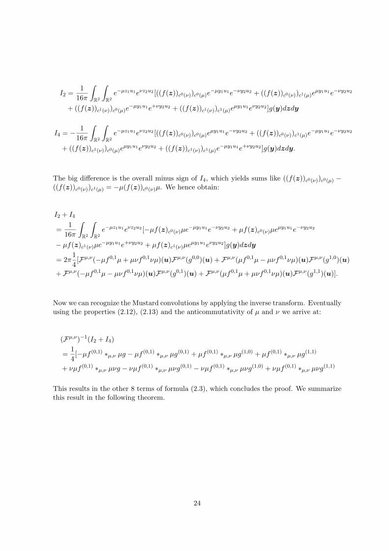
The big difference is the overall minus sign of I4, which yields sums like ((f(z))c0(ν))c0(µ) −((f(z))c0(ν))c1(µ) = −µ(f(z))c0(ν)µ. We hence obtain:

I2 + I4

=1

16π

∫R2

∫R2

e−µz1u1eνz2u2 [−µf(z)c0(ν)µe−µy1u1e−νy2u2 + µf(z)c0(ν)µe

µy1u1e−νy2u2

− µf(z)c1(ν)µe−µy1u1e+νy2u2 + µf(z)c1(ν)µe

µy1u1eνy2u2 ]g(y)dzdy

= 2π1

4[Fµ,ν(−µf0,1µ+ µνf0,1νµ)(u)Fµ,ν(g0,0)(u) + Fµ,ν(µf0,1µ− µνf0,1νµ)(u)Fµ,ν(g1,0)(u)

+ Fµ,ν(−µf0,1µ− µνf0,1νµ)(u)Fµ,ν(g0,1)(u) + Fµ,ν(µf0,1µ+ µνf0,1νµ)(u)Fµ,ν(g1,1)(u)].

Now we can recognize the Mustard convolutions by applying the inverse transform. Eventuallyusing the properties (2.12), (2.13) and the anticommutativity of µ and ν we arrive at:

(Fµ,ν)−1(I2 + I4)

=1

4[−µf (0,1) ∗µ,ν µg − µf (0,1) ∗µ,ν µg(0,1) + µf (0,1) ∗µ,ν µg(1,0) + µf (0,1) ∗µ,ν µg(1,1)

+ νµf (0,1) ∗µ,ν µνg − νµf (0,1) ∗µ,ν µνg(0,1) − νµf (0,1) ∗µ,ν µνg(1,0) + νµf (0,1) ∗µ,ν µνg(1,1)

This results in the other 8 terms of formula (2.3), which concludes the proof. We summarizethis result in the following theorem.

24

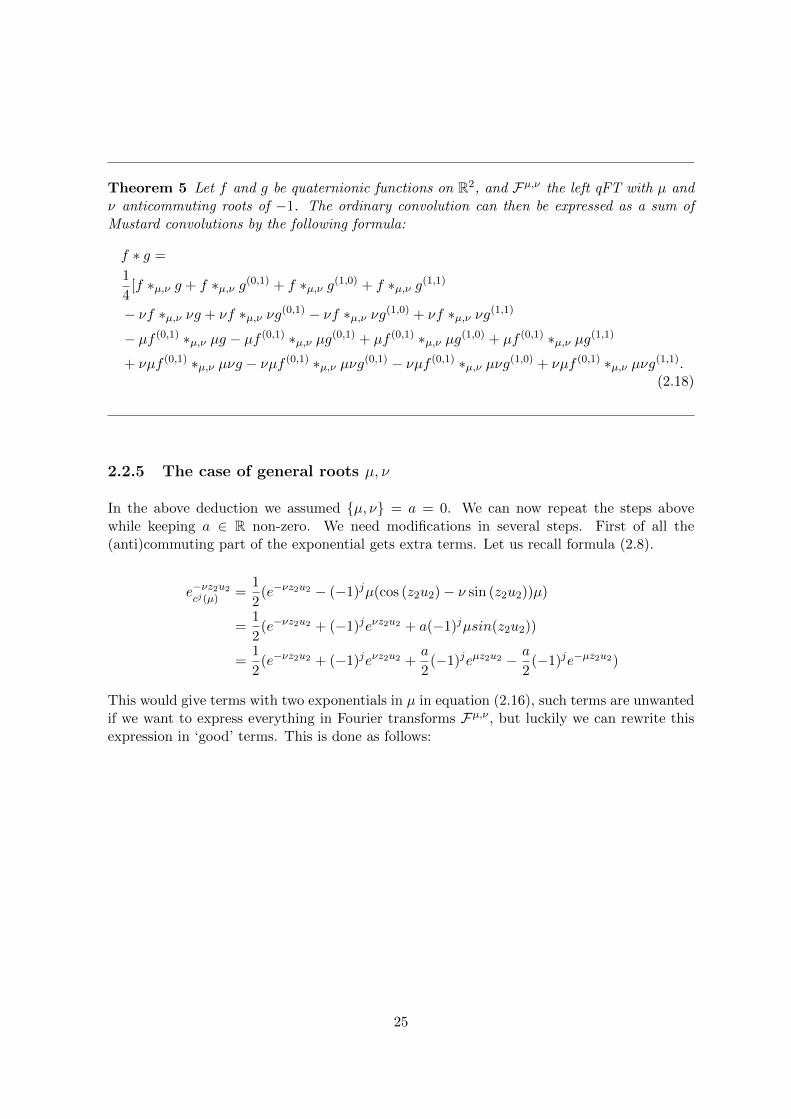
Theorem 5 Let f and g be quaternionic functions on R2, and Fµ,ν the left qFT with µ andν anticommuting roots of −1. The ordinary convolution can then be expressed as a sum ofMustard convolutions by the following formula:

f ∗ g =

1

4[f ∗µ,ν g + f ∗µ,ν g(0,1) + f ∗µ,ν g(1,0) + f ∗µ,ν g(1,1)

− νf ∗µ,ν νg + νf ∗µ,ν νg(0,1) − νf ∗µ,ν νg(1,0) + νf ∗µ,ν νg(1,1)

− µf (0,1) ∗µ,ν µg − µf (0,1) ∗µ,ν µg(0,1) + µf (0,1) ∗µ,ν µg(1,0) + µf (0,1) ∗µ,ν µg(1,1)

+ νµf (0,1) ∗µ,ν µνg − νµf (0,1) ∗µ,ν µνg(0,1) − νµf (0,1) ∗µ,ν µνg(1,0) + νµf (0,1) ∗µ,ν µνg(1,1).(2.18)

2.2.5 The case of general roots µ, ν

In the above deduction we assumed {µ, ν} = a = 0. We can now repeat the steps abovewhile keeping a ∈ R non-zero. We need modifications in several steps. First of all the(anti)commuting part of the exponential gets extra terms. Let us recall formula (2.8).

e−νz2u2cj(µ)

=1

2(e−νz2u2 − (−1)jµ(cos (z2u2)− ν sin (z2u2))µ)

=1

2(e−νz2u2 + (−1)jeνz2u2 + a(−1)jµsin(z2u2))

=1

2(e−νz2u2 + (−1)jeνz2u2 +

a

2(−1)jeµz2u2 − a

2(−1)je−µz2u2)

This would give terms with two exponentials in µ in equation (2.16), such terms are unwantedif we want to express everything in Fourier transforms Fµ,ν , but luckily we can rewrite thisexpression in ‘good’ terms. This is done as follows:

25

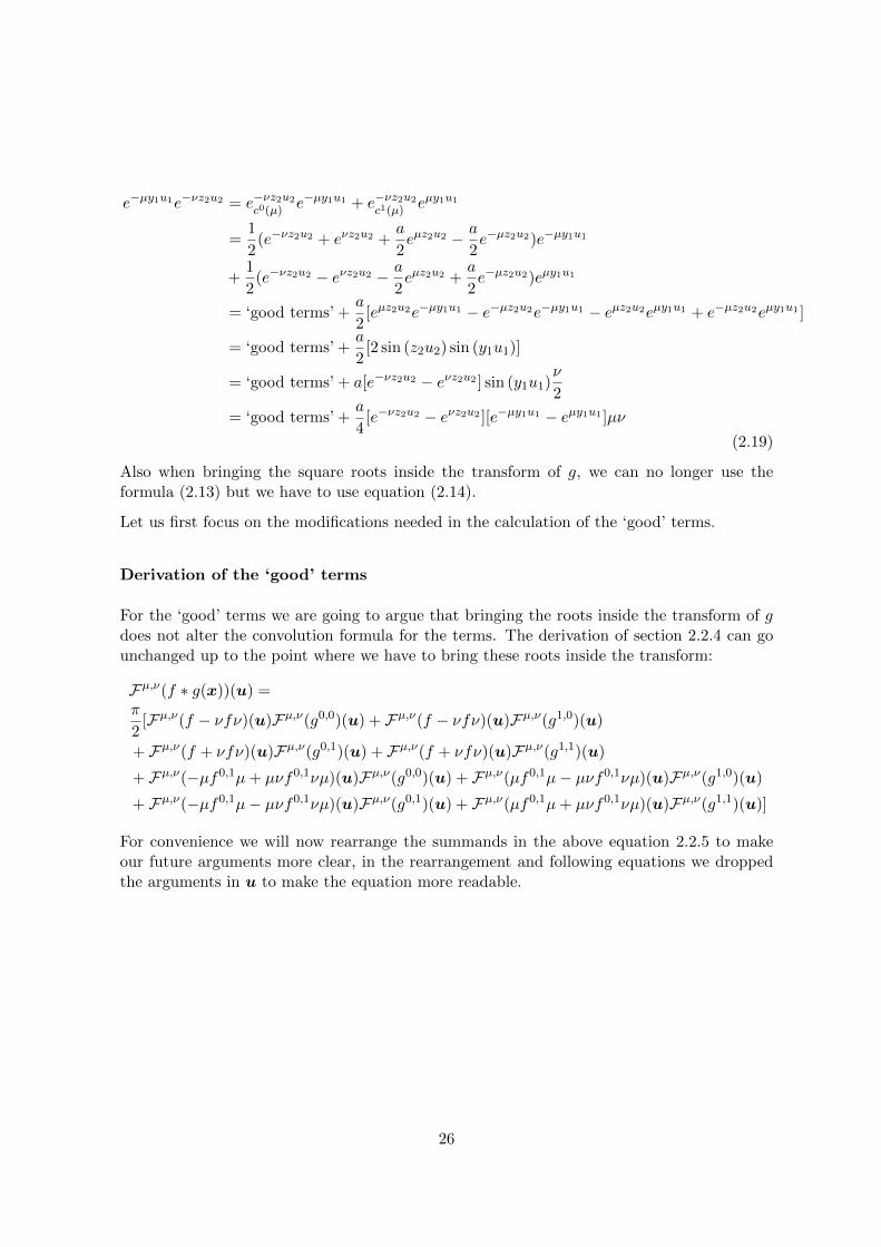
e−µy1u1e−νz2u2 = e−νz2u2c0(µ)

e−µy1u1 + e−νz2u2c1(µ)

eµy1u1

=1

2(e−νz2u2 + eνz2u2 +

a

2eµz2u2 − a

2e−µz2u2)e−µy1u1

+1

2(e−νz2u2 − eνz2u2 − a

2eµz2u2 +

a

2e−µz2u2)eµy1u1

= ‘good terms’ +a

2[eµz2u2e−µy1u1 − e−µz2u2e−µy1u1 − eµz2u2eµy1u1 + e−µz2u2eµy1u1 ]

= ‘good terms’ +a

2[2 sin (z2u2) sin (y1u1)]

= ‘good terms’ + a[e−νz2u2 − eνz2u2 ] sin (y1u1)ν

2

= ‘good terms’ +a

4[e−νz2u2 − eνz2u2 ][e−µy1u1 − eµy1u1 ]µν

(2.19)

Also when bringing the square roots inside the transform of g, we can no longer use theformula (2.13) but we have to use equation (2.14).

Let us first focus on the modifications needed in the calculation of the ‘good’ terms.

Derivation of the ‘good’ terms

For the ‘good’ terms we are going to argue that bringing the roots inside the transform of gdoes not alter the convolution formula for the terms. The derivation of section 2.2.4 can gounchanged up to the point where we have to bring these roots inside the transform:

Fµ,ν(f ∗ g(x))(u) =π

2[Fµ,ν(f − νfν)(u)Fµ,ν(g0,0)(u) + Fµ,ν(f − νfν)(u)Fµ,ν(g1,0)(u)

+ Fµ,ν(f + νfν)(u)Fµ,ν(g0,1)(u) + Fµ,ν(f + νfν)(u)Fµ,ν(g1,1)(u)

+ Fµ,ν(−µf0,1µ+ µνf0,1νµ)(u)Fµ,ν(g0,0)(u) + Fµ,ν(µf0,1µ− µνf0,1νµ)(u)Fµ,ν(g1,0)(u)

+ Fµ,ν(−µf0,1µ− µνf0,1νµ)(u)Fµ,ν(g0,1)(u) + Fµ,ν(µf0,1µ+ µνf0,1νµ)(u)Fµ,ν(g1,1)(u)]

For convenience we will now rearrange the summands in the above equation 2.2.5 to makeour future arguments more clear, in the rearrangement and following equations we droppedthe arguments in u to make the equation more readable.

26

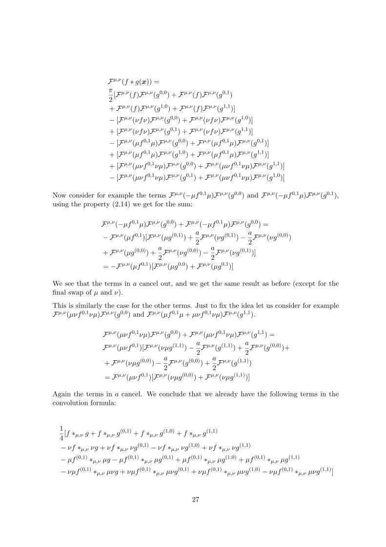
Fµ,ν(f ∗ g(x)) =π

2[Fµ,ν(f)Fµ,ν(g0,0) + Fµ,ν(f)Fµ,ν(g0,1)

+ Fµ,ν(f)Fµ,ν(g1,0) + Fµ,ν(f)Fµ,ν(g1,1)]

− [Fµ,ν(νfν)Fµ,ν(g0,0) + Fµ,ν(νfν)Fµ,ν(g1,0)]

+ [Fµ,ν(νfν)Fµ,ν(g0,1) + Fµ,ν(νfν)Fµ,ν(g1,1)]

− [Fµ,ν(µf0,1µ)Fµ,ν(g0,0) + Fµ,ν(µf0,1µ)Fµ,ν(g0,1)]

+ [Fµ,ν(µf0,1µ)Fµ,ν(g1,0) + Fµ,ν(µf0,1µ)Fµ,ν(g1,1)]

+ [Fµ,ν(µνf0,1νµ)Fµ,ν(g0,0) + Fµ,ν(µνf0,1νµ)Fµ,ν(g1,1)]

− [Fµ,ν(µνf0,1νµ)Fµ,ν(g0,1) + Fµ,ν(µνf0,1νµ)Fµ,ν(g1,0)]

Now consider for example the terms Fµ,ν(−µf0,1µ)Fµ,ν(g0,0) and Fµ,ν(−µf0,1µ)Fµ,ν(g0,1),using the property (2.14) we get for the sum:

Fµ,ν(−µf0,1µ)Fµ,ν(g0,0) + Fµ,ν(−µf0,1µ)Fµ,ν(g0,0) =

−Fµ,ν(µf0,1)[Fµ,ν(µg(0,1)) +a

2Fµ,ν(νg(0,1))− a

2Fµ,ν(νg(0,0))

+ Fµ,ν(µg(0,0)) +a

2Fµ,ν(νg(0,0))− a

2Fµ,ν(νg(0,1))]

= −Fµ,ν(µf0,1)[Fµ,ν(µg0,0) + Fµ,ν(µg0,1)]

We see that the terms in a cancel out, and we get the same result as before (except for thefinal swap of µ and ν).

This is similarly the case for the other terms. Just to fix the idea let us consider for exampleFµ,ν(µνf0,1νµ)Fµ,ν(g0,0) and Fµ,ν(µf0,1µ+ µνf0,1νµ)Fµ,ν(g1,1).

Fµ,ν(µνf0,1νµ)Fµ,ν(g0,0) + Fµ,ν(µνf0,1νµ)Fµ,ν(g1,1) =

Fµ,ν(µνf0,1)[Fµ,ν(νµg(1,1))− a

2Fµ,ν(g(1,1)) +

a

2Fµ,ν(g(0,0))+

+ Fµ,ν(νµg(0,0))− a

2Fµ,ν(g(0,0)) +

a

2Fµ,ν(g(1,1))

= Fµ,ν(µνf0,1)[Fµ,ν(νµg(0,0)) + Fµ,ν(νµg(1,1))]

Again the terms in a cancel. We conclude that we already have the following terms in theconvolution formula:

1

4[f ∗µ,ν g + f ∗µ,ν g(0,1) + f ∗µ,ν g(1,0) + f ∗µ,ν g(1,1)

− νf ∗µ,ν νg + νf ∗µ,ν νg(0,1) − νf ∗µ,ν νg(1,0) + νf ∗µ,ν νg(1,1)

− µf (0,1) ∗µ,ν µg − µf (0,1) ∗µ,ν µg(0,1) + µf (0,1) ∗µ,ν µg(1,0) + µf (0,1) ∗µ,ν µg(1,1)

− νµf (0,1) ∗µ,ν µνg + νµf (0,1) ∗µ,ν µνg(0,1) + νµf (0,1) ∗µ,ν µνg(1,0) − νµf (0,1) ∗µ,ν µνg(1,1)]

27

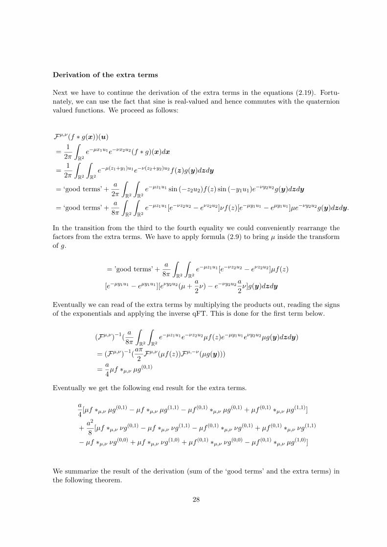
Derivation of the extra terms

Next we have to continue the derivation of the extra terms in the equations (2.19). Fortu-nately, we can use the fact that sine is real-valued and hence commutes with the quaternionvalued functions. We proceed as follows:

Fµ,ν(f ∗ g(x))(u)

=1

2π

∫R2

e−µx1u1e−νx2u2(f ∗ g)(x)dx

=1

2π

∫R2

∫R2

e−µ(z1+y1)u1e−ν(z2+y2)u2f(z)g(y)dzdy

= ‘good terms’ +a

2π

∫R2

∫R2

e−µz1u1 sin (−z2u2)f(z) sin (−y1u1)e−νy2u2g(y)dzdy

= ‘good terms’ +a

8π

∫R2

∫R2

e−µz1u1 [e−νz2u2 − eνz2u2 ]νf(z)[e−µy1u1 − eµy1u1 ]µe−νy2u2g(y)dzdy.

In the transition from the third to the fourth equality we could conveniently rearrange thefactors from the extra terms. We have to apply formula (2.9) to bring µ inside the transformof g.

= ’good terms’ +a

8π

∫R2

∫R2

e−µz1u1 [e−νz2u2 − eνz2u2 ]µf(z)

[e−µy1u1 − eµy1u1 ][eνy2u2(µ+a

2ν)− e−νy2u2 a

2ν]g(y)dzdy

Eventually we can read of the extra terms by multiplying the products out, reading the signsof the exponentials and applying the inverse qFT. This is done for the first term below.

(Fµ,ν)−1(a

8π

∫R2

∫R2

e−µz1u1e−νz2u2µf(z)e−µy1u1eνy2u2µg(y)dzdy)

= (Fµ,ν)−1(aπ

2Fµ,ν(µf(z))Fµ,−ν(µg(y)))

=a

4µf ∗µ,ν µg(0,1)

Eventually we get the following end result for the extra terms.

a

4[µf ∗µ,ν µg(0,1) − µf ∗µ,ν µg(1,1) − µf (0,1) ∗µ,ν µg(0,1) + µf (0,1) ∗µ,ν µg(1,1)]

+a2

8[µf ∗µ,ν νg(0,1) − µf ∗µ,ν νg(1,1) − µf (0,1) ∗µ,ν νg(0,1) + µf (0,1) ∗µ,ν νg(1,1)

− µf ∗µ,ν νg(0,0) + µf ∗µ,ν νg(1,0) + µf (0,1) ∗µ,ν νg(0,0) − µf (0,1) ∗µ,ν µg(1,0)]

We summarize the result of the derivation (sum of the ‘good terms’ and the extra terms) inthe following theorem.

28

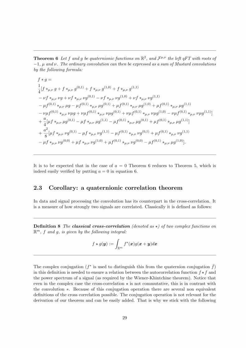
Theorem 6 Let f and g be quaternionic functions on R2, and Fµ,ν the left qFT with roots of−1, µ and ν. The ordinary convolution can then be expressed as a sum of Mustard convolutionsby the following formula:

f ∗ g =

1

4[f ∗µ,ν g + f ∗µ,ν g(0,1) + f ∗µ,ν g(1,0) + f ∗µ,ν g(1,1)

− νf ∗µ,ν νg + νf ∗µ,ν νg(0,1) − νf ∗µ,ν νg(1,0) + νf ∗µ,ν νg(1,1)

− µf (0,1) ∗µ,ν µg − µf (0,1) ∗µ,ν µg(0,1) + µf (0,1) ∗µ,ν µg(1,0) + µf (0,1) ∗µ,ν µg(1,1)

− νµf (0,1) ∗µ,ν νµg + νµf (0,1) ∗µ,ν νµg(0,1) + νµf (0,1) ∗µ,ν νµg(1,0) − νµf (0,1) ∗µ,ν νµg(1,1)]

+a

4[µf ∗µ,ν µg(0,1) − µf ∗µ,ν µg(1,1) − µf (0,1) ∗µ,ν µg(0,1) + µf (0,1) ∗µ,ν µg(1,1)]

+a2

8[µf ∗µ,ν νg(0,1) − µf ∗µ,ν νg(1,1) − µf (0,1) ∗µ,ν νg(0,1) + µf (0,1) ∗µ,ν νg(1,1)

− µf ∗µ,ν νg(0,0) + µf ∗µ,ν νg(1,0) + µf (0,1) ∗µ,ν νg(0,0) − µf (0,1) ∗µ,ν µg(1,0)].

It is to be expected that in the case of a = 0 Theorem 6 reduces to Theorem 5, which isindeed easily verified by putting a = 0 in equation 6.

2.3 Corollary: a quaternionic correlation theorem

In data and signal processing the convolution has its counterpart in the cross-correlation. Itis a measure of how strongly two signals are correlated. Classically it is defined as follows:

Definition 8 The classical cross-correlation (denoted as ?) of two complex functions onRm, f and g, is given by the following integral:

f ? g(y) :=

∫Rm

f∗(x)g(x+ y)dx

The complex conjugation (f∗ is used to distinguish this from the quaternion conjugation f)in this definition is needed to ensure a relation between the autocorrelation function f ?f andthe power spectrum of a signal (as required by the Wiener-Khintchine theorem). Notice thateven in the complex case the cross-correlation ? is not commutative, this is in contrast withthe convolution ∗. Because of this conjugation operation there are several non equivalentdefinitions of the cross correlation possible. The conjugation operation is not relevant for thederivation of our theorem and can be easily added. That is why we stick with the following

29

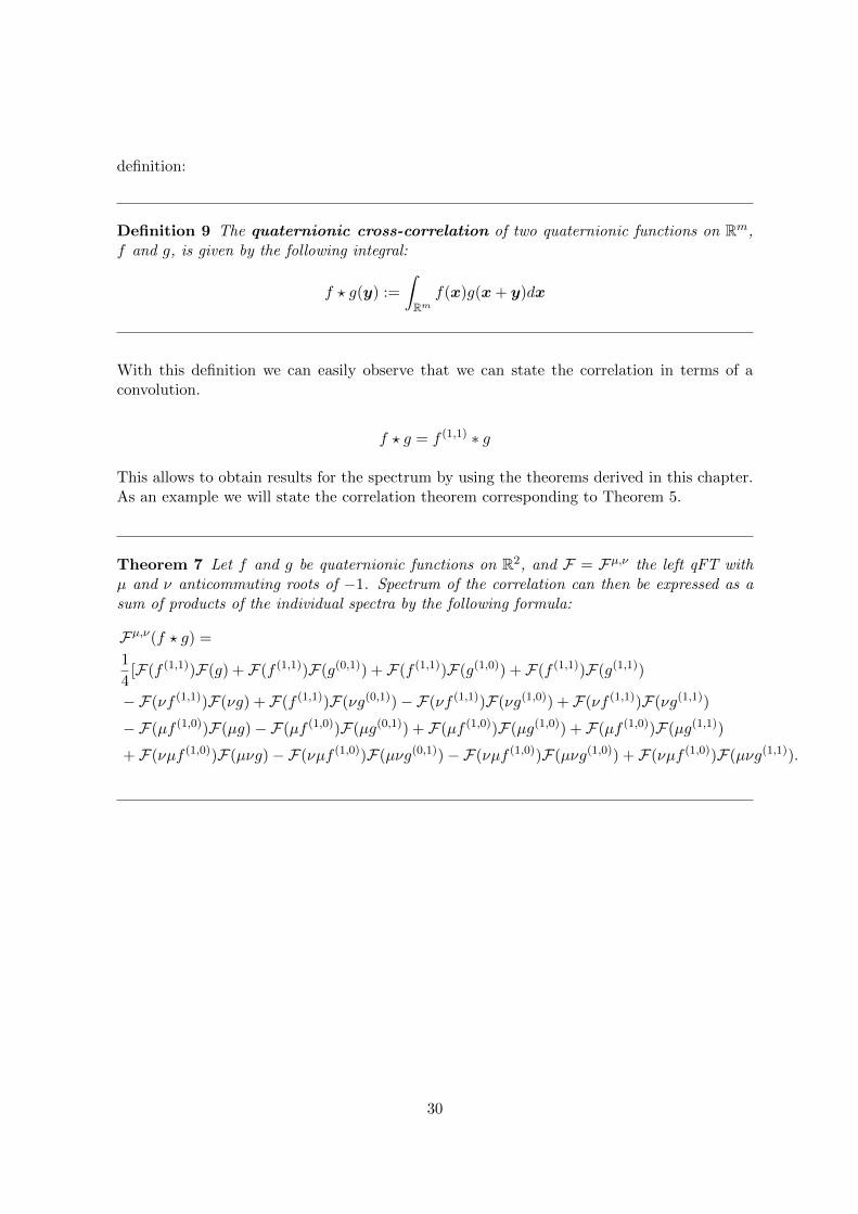
definition:

Definition 9 The quaternionic cross-correlation of two quaternionic functions on Rm,f and g, is given by the following integral:

f ? g(y) :=

∫Rm

f(x)g(x+ y)dx

With this definition we can easily observe that we can state the correlation in terms of aconvolution.

f ? g = f (1,1) ∗ g

This allows to obtain results for the spectrum by using the theorems derived in this chapter.As an example we will state the correlation theorem corresponding to Theorem 5.

Theorem 7 Let f and g be quaternionic functions on R2, and F = Fµ,ν the left qFT withµ and ν anticommuting roots of −1. Spectrum of the correlation can then be expressed as asum of products of the individual spectra by the following formula:

Fµ,ν(f ? g) =

1

4[F(f (1,1))F(g) + F(f (1,1))F(g(0,1)) + F(f (1,1))F(g(1,0)) + F(f (1,1))F(g(1,1))

−F(νf (1,1))F(νg) + F(f (1,1))F(νg(0,1))−F(νf (1,1))F(νg(1,0)) + F(νf (1,1))F(νg(1,1))

−F(µf (1,0))F(µg)−F(µf (1,0))F(µg(0,1)) + F(µf (1,0))F(µg(1,0)) + F(µf (1,0))F(µg(1,1))

+ F(νµf (1,0))F(µνg)−F(νµf (1,0))F(µνg(0,1))−F(νµf (1,0))F(µνg(1,0)) + F(νµf (1,0))F(µνg(1,1)).

30

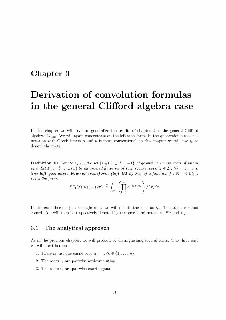
Chapter 3

Derivation of convolution formulasin the general Clifford algebra case

In this chapter we will try and generalize the results of chapter 2 to the general Cliffordalgebras Cl0,m. We will again concentrate on the left transform. In the quaternionic case thenotation with Greek letters µ and ν is more conventional, in this chapter we will use ik todenote the roots.

Definition 10 Denote by Im the set {i ∈ Cl0,m|i2 = −1} of geometric square roots of minusone. Let F1 := {i1, ..., im} be an ordered finite set of such square roots, ik ∈ Im,∀k = 1, ...,m.The left geometric Fourier transform (left GFT) FF1 of a function f : Rm → Cl0,mtakes the form:

FF1(f)(u) := (2π)−m2

∫Rm

(m∏k=1

e−ikxkuk

)f(x)dx.

In the case there is just a single root, we will denote the root as is. The transform andconvolution will then be respectively denoted by the shorthand notations F is and ∗is .

3.1 The analytical approach

As in the previous chapter, we will proceed by distinguishing several cases. The three casewe will treat here are:

1. There is just one single root ik = is∀k ∈ {1, . . . ,m}

2. The roots ik are pairwise anticommuting

3. The roots ik are pairwise coorthogonal

31

3.1.1 The case of a single root ik = is

This case is quite similar to the quaternionic case. We start of by applying the usual steps.

F i(f ∗ g(x))(u) = (2π)−m2

∫Rm

m∏k=1

e−isxkuk(f ∗ g)(x)dx

= (2π)−m2

∫Rm

m∏k=1

e−isxkuk∫R2

f(x− y)g(y)dydx

= (2π)−m2

∫Rm

∫Rm

e−is∑mk=1 xkukf(x− y)g(y)dydx

= (2π)−m2

∫Rm

∫Rm

e−is∑mk=1(zk+yk)ukf(z)g(y)dzdy

= (2π)−m2

∫Rm

∫Rm

e−is∑mk=1 zkuke−is

∑mk=1 ykukf(z)g(y)dzdy

Again there is just one root, so we can swap the exponentials. We continue by pulling fthrough the exponentials.

F i(f ∗ g(x))(u)

=1

2π

∫Rm

∫Rm

e−is∑mk=1 zkuk [f(z)c0(is)e

−is∑mk=1 ykuk + f(z)c1(is)e

is∑mk=1 ykuk ]g(y)dzdy

=1

2

1

2π

∫Rm

∫Rm

e−is∑mk=1 zkuk [(f(z)− isf(z)is)e

−is∑mk=1 ykuk + (f(z) + isf(z)is)e

is∑mk=1 ykuk ]g(y)dzdy

=1

2

1

2π

∫Rm

∫Rm

e−is∑mk=1 zkukf(z)e−i

∑mk=1 ykukg(y)− e−is

∑mk=1 zkukisf(z)e−is

∑mk=1 ykukisg(y)

+ e−is∑mk=1 zkukf(z)e−is

∑mk=1 ykukg(y) + e−is

∑mk=1 zkukisf(z)e−is

∑mk=1 ykukisg(y)dzdy

=1

22π[F is(f)(u)F is(g)(u)−F is(isf)(u)F is(isg)(u)

+ F is(f)(u)F is(g(1,1))(u) + F is(isf)(u)F is(isg(1,1))(u)]

In a final step we apply the inverse Fourier transform to both sides, yielding

f ∗ g(x) =1

2[f ∗is g − isf ∗is isg + f ∗is g(1,1,...,1) + if ∗is ig(1,1,...,1)]

Let us clarify again the notation we introduced in chapters 1 and 2 for the change of signs:

NotationFor functions f, g : Rm → Cl0,m and multi-indices φ,γ ∈ {0, 1}m we put

fφ(x) := f((−1)φ1x1, ..., (−1)φmxm),

gγ(x) := g((−1)γ1x1, ..., (−1)γmxm).

32

Later on we could for example encounter form = 4 a term with a function like f (1,0,1,0)(x1, x2, x3, x4) =f(−x1, x2,−x3, x4). Here in our case this notation means that we have that g(1,1,...,1)(x1, x2, . . . , xm) =g(1,1,...,1)(−x1,−x2, . . . ,−xm).

We can conclude with the following theorem:

Theorem 9 Let f and g be Clifford valued functions on Rm, and F is the left GFT with isa single root of −1. The ordinary convolution can then be expressed as a sum of Mustardconvolutions by the following formula:

f ∗ g(x) =1

2[f ∗is g − isf ∗is isg + f ∗is g(1,1,...,1) + if ∗is ig(1,1,...,1)]

3.1.2 The case of pairwise anticommuting roots ik

We will now focus on a more general case of the transform. Where the roots ik are pairwiseanticommuting: {ik, il} = −2δkl with k, l ∈ {0, . . . ,m}. To make the long procedure ofderiving this formula a bit more clear we proceed in several steps.

1. Usual preparatory steps: bringing the integrals to the outside (Fubini’s theorem) andthe substitution x→ z + y

2. Reordering of the exponentials∏mk=1 e

−ik(zk+yk)uk

3. Split of the function f

4. Separating factors in y and z

5. Identification of the geometric Fourier transforms

6. Further reduction of the formula

7. Finally we also check the formula in the quaternionic case

When the derivation is finished we will also verify the quaternionic case from the generalformula.

1. Preparatory steps

The procedure of the usual steps should be clear by now to the reader.

33

FF1(f ∗ g(x))(u) = (2π)−m2

∫Rm

m∏k=1

e−ikxkuk(f ∗ g)(x)dx

= (2π)−m2

∫Rm

m∏k=1

e−ikxkuk∫R2

f(x− y)g(y)dydx

= (2π)−m2

∫Rm

∫Rm

m∏k=1

e−ikxkukf(x− y)g(y)dydx

= (2π)−m2

∫Rm

∫Rm

m∏k=1

e−ik(zk+yk)ukf(z)g(y)dzdy

(3.1)

2. Reordering of the exponentials∏mk=1 e

−ik(zk+yk)uk

While in the previous case in section 3.1.1 the reordering of the ordered product∏mk=1 e

−ik(zk+yk)uk

was trivial, here this will no longer be the case. In the other cases we did not really have todeal with the problem of products

∏of non commuting Clifford numbers, here we will have

to treat these ordered products with care. That is why we will clarify what we mean by anordered product of Clifford numbers. Let I be the set of labels {1, . . . , l}, then we define:

l∏k=1

ak =∏k∈I

:=−→∏k∈I

= a1a2 . . . al. (3.2)

This means that by convention we will always start with the first label on the leftside of theproduct. Because we will have to reorder these ordered products, we will also need a notationfor a permuted product. If we consider a certain permutation ρ on l elements then we define:

∏k∈ρ

ak :=−−−→∏k∈ρ(I)

ak =∏

k∈{ρ1,...,ρl}

ak = aρ1aρ2 . . . aρl. (3.3)

Just like in the quaternionic case (m = 2) of anticommuting roots in section 2.2.4, we have toapply a procedure to reorder the exponentials. Because of simplicity we opted to work withthe commuting and anticommuting parts of exponentials for the case m = 2. Here we chooseto take an other approach based on the notation used in [7]:

e−ikzkukjk:=

{cos(zkuk), if jk = 0,

− sin(zkuk), if jk = 1.(3.4)

For convenience we also introduce the notations θk and ik with k ∈ {1, . . . , 2m} for theargument of the exponentials:

34

θk :=

z k+12u k+1

2if k is odd,

y k2u k

2if k is even.

,

i′k :=

i k+12

if k is odd,

i k2

if k is even.and

m∏k=1

e−ik(zk+yk)uk =2m∏k=1

e−i′kθk ,

making the row of arguments (θk)2mk=1 = (z1u1, y1u1, z2u2, y2u2, . . . , zm, ym) and roots (i′k)

2mk=1 =

(i1, i1, i2, i2, . . . , im, im) less bothersome.

The notation (3.4) allows us to write:

e−i′kθk =

1∑jk=0

(i′k)jke−i′kθkjk

and

2m∏k=1

e−i′kθk =

∑j∈{0,1}2m

2m∏k=1

(i′k)jke−i′kθkjk

,

where the sum in the last equation is over all possible vectors j in {0, 1}2m.

The advantage of this notation is that the factors e−i′kθkjk

are scalars and in the center ofthe algebra, they commute with everything. This means that the rearrangement of theexponentials boils down to the rearrangement of the roots

∏2mk=1(i

′k)jk . Because these roots

are pairwise anticommuting this rearrangement will only yield a different sign. This sign willbe determined by the presence of the roots in the product or with other words the vector j.We want the separation of the exponentials in z and in y, so we want the arguments to berearranged as follows:

ρ : (z1, y1, z2, y2, . . . , zm, ym) 7→ (z1, z2, . . . , zm, y1, y2, . . . , ym)

This is in fact the inverse of the perfect shuffle permutation, it concerns a so called out shufflebecause the first element stays the first element after the shuffle. It is a well known fact thatany permutation can be factorized in terms of transpositions. Therefore we will first studythe effect of a transposition Tl,l+1 = (l l + 1) of two roots in

∏2mk=1(i

′k)jk , and derive the

effect of the total permutation from this.

Let us consider the swap of (i′l)jl(i′l+1)

jl+1. It is clear that an actual swap will only take placewhen both roots are present (jl = 1, jl+1 = 1) and when the roots are not equal i′l 6= i′l+1.The transposition introduces the following change of sign:

35

(i′l)jl(i′l+1)

jl+1 = (−1)κl,l+1(i′l+1)jl+1(i′l)

jl∏k∈I

(i′k)jk = (−1)κl,l+1

∏k∈Tl,l+1

(i′k)jk with κr,s := jrjs(1 +

{i′r, i′s}2

).

(3.5)

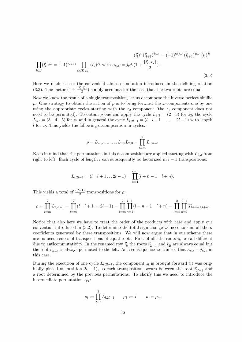
Here we made use of the convenient abuse of notation introduced in the defining relation

(3.3). The factor (1 + {i′r,i′s}2 ) simply accounts for the case that the two roots are equal.

Now we know the result of a single transposition, let us decompose the inverse perfect shuffleρ. One strategy to obtain the action of ρ is to bring forward the z-components one by oneusing the appropriate cycles starting with the z2 component (the z1 component does notneed to be permuted). To obtain ρ one can apply the cycle L2,3 = (2 3) for z2, the cycleL3,5 = (3 4 5) for z3 and in general the cycle Ll,2l−1 = (l l+ 1 . . . 2l− 1) with lengthl for zl. This yields the following decomposition in cycles:

ρ = Lm,2m−1 . . . L3,5L2,3 =2∏

l=m

Ll,2l−1

Keep in mind that the permutations in this decomposition are applied starting with L2,3 fromright to left. Each cycle of length l can subsequently be factorized in l − 1 transpositions:

Ll,2l−1 = (l l + 1 . . . 2l − 1) =l−1∏n=1

(l + n− 1 l + n).

This yields a total of l(l−1)2 transpositions for ρ:

ρ =2∏

l=m

Ll,2l−1 =2∏

l=m

(l l + 1 . . . 2l − 1) =2∏

l=m

l−1∏n=1

(l + n− 1 l + n) =2∏

l=m

l−1∏n=1

Tl+n−1,l+n.

Notice that also here we have to treat the order of the products with care and apply ourconvention introduced in (3.2). To determine the total sign change we need to sum all the κcoefficients generated by these transpositions. We will now argue that in our scheme thereare no occurrences of transpositions of equal roots. First of all, the roots ik are all differentdue to anticommutativity. In the renamed row i′k the roots i′2l−1 and i′2l are always equal butthe root i′2l−1 is always permuted to the left. As a consequence we can see that κr,s = jrjs inthis case.

During the execution of one cycle Ll,2l−1, the component zl is brought forward (it was orig-inally placed on position 2l − 1), so each transposition occurs between the root i′2l−1 anda root determined by the previous permutations. To clarify this we need to introduce theintermediate permutations ρt:

ρt :=2∏l=t

Ll,2l−1 ρ1 := I ρ := ρm

36

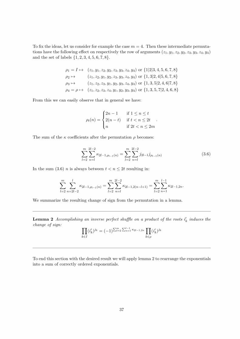
To fix the ideas, let us consider for example the case m = 4. Then these intermediate permuta-tions have the following effect on respectively the row of arguments (z1, y1, z2, y2, z3, y3, z4, y4)and the set of labels {1, 2, 3, 4, 5, 6, 7, 8}.

ρ1 = I 7→ (z1, y1, z2, y2, z3, y3, z4, y4) or {1|2|3, 4, 5, 6, 7, 8}ρ2 7→ (z1, z2, y1, y2, z3, y3, z4, y4) or {1, 3|2, 4|5, 6, 7, 8}ρ3 7→ (z1, z2, z3, y1, y2, y3, z4, y4) or {1, 3, 5|2, 4, 6|7, 8}ρ4 = ρ 7→ (z1, z2, z3, z4, y1, y2, y3, y4) or {1, 3, 5, 7|2, 4, 6, 8}

From this we can easily observe that in general we have:

ρt(n) =

2n− 1 if 1 ≤ n ≤ t2(n− t) if t < n ≤ 2t

n if 2t < n ≤ 2m

.

The sum of the κ coefficients after the permutation ρ becomes:

m∑l=2

2l−2∑n=l

κ2l−1,ρl−1(n) =m∑l=2

2l−2∑n=l

j2l−1jρl−1(n) (3.6)

In the sum (3.6) n is always between t < n ≤ 2t resulting in:

m∑l=2

l∑n=2l−2

κ2l−1,ρl−1(n) =

m∑l=2

2l−2∑n=l

κ2l−1,2(n−l+1) =

m∑l=2

l−1∑n=1

κ2l−1,2n.

We summarize the resulting change of sign from the permutation in a lemma.

Lemma 2 Accomplishing an inverse perfect shuffle on a product of the roots i′k induces thechange of sign: ∏

k∈I(i′k)

jk = (−1)∑ml=2

∑l−1n=1 κ2l−1,2n

∏k∈ρ

(i′k)jk

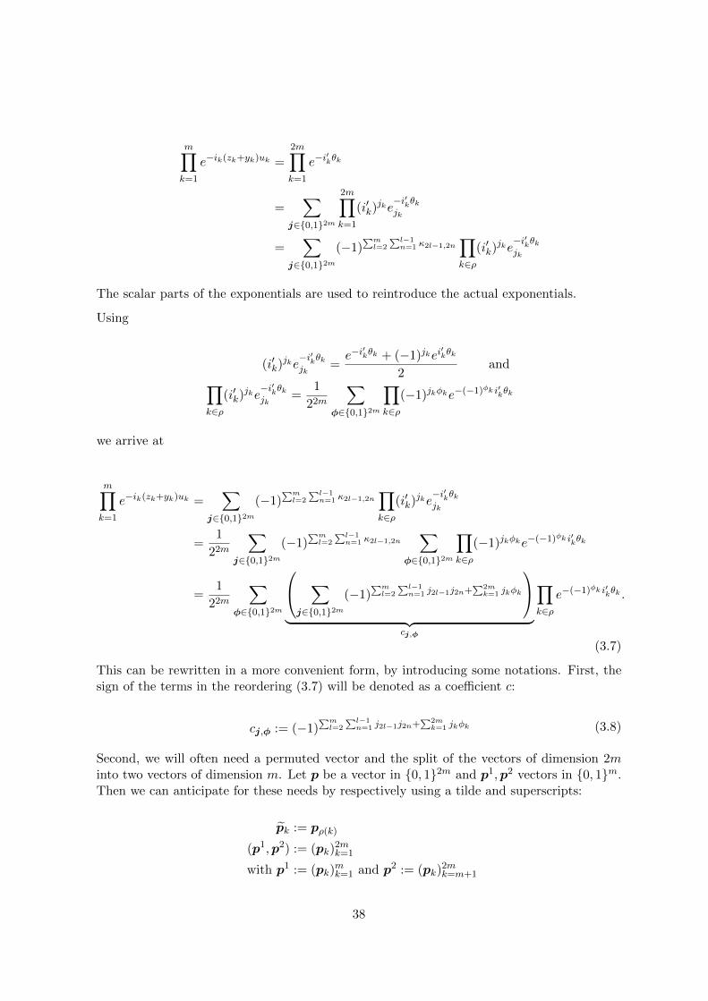
To end this section with the desired result we will apply lemma 2 to rearrange the exponentialsinto a sum of correctly ordered exponentials.

37

m∏k=1

e−ik(zk+yk)uk =

2m∏k=1

e−i′kθk

=∑

j∈{0,1}2m

2m∏k=1

(i′k)jke−i′kθkjk

=∑

j∈{0,1}2m(−1)

∑ml=2

∑l−1n=1 κ2l−1,2n

∏k∈ρ

(i′k)jke−i′kθkjk

The scalar parts of the exponentials are used to reintroduce the actual exponentials.

Using

(i′k)jke−i′kθkjk

=e−i′kθk + (−1)jkei

′kθk

2and∏

k∈ρ(i′k)

jke−i′kθkjk

=1

22m

∑φ∈{0,1}2m

∏k∈ρ

(−1)jkφke−(−1)φk i′kθk

we arrive at

m∏k=1

e−ik(zk+yk)uk =∑

j∈{0,1}2m(−1)

∑ml=2

∑l−1n=1 κ2l−1,2n

∏k∈ρ

(i′k)jke−i′kθkjk

=1

22m

∑j∈{0,1}2m

(−1)∑ml=2

∑l−1n=1 κ2l−1,2n

∑φ∈{0,1}2m

∏k∈ρ

(−1)jkφke−(−1)φk i′kθk

=1

22m

∑φ∈{0,1}2m

∑j∈{0,1}2m

(−1)∑ml=2

∑l−1n=1 j2l−1j2n+

∑2mk=1 jkφk

︸ ︷︷ ︸

cj,φ

∏k∈ρ

e−(−1)φk i′kθk .

(3.7)

This can be rewritten in a more convenient form, by introducing some notations. First, thesign of the terms in the reordering (3.7) will be denoted as a coefficient c:

cj,φ := (−1)∑ml=2

∑l−1n=1 j2l−1j2n+

∑2mk=1 jkφk (3.8)

Second, we will often need a permuted vector and the split of the vectors of dimension 2minto two vectors of dimension m. Let p be a vector in {0, 1}2m and p1,p2 vectors in {0, 1}m.Then we can anticipate for these needs by respectively using a tilde and superscripts:

pk := pρ(k)

(p1,p2) := (pk)2mk=1

with p1 := (pk)mk=1 and p2 := (pk)

2mk=m+1

38

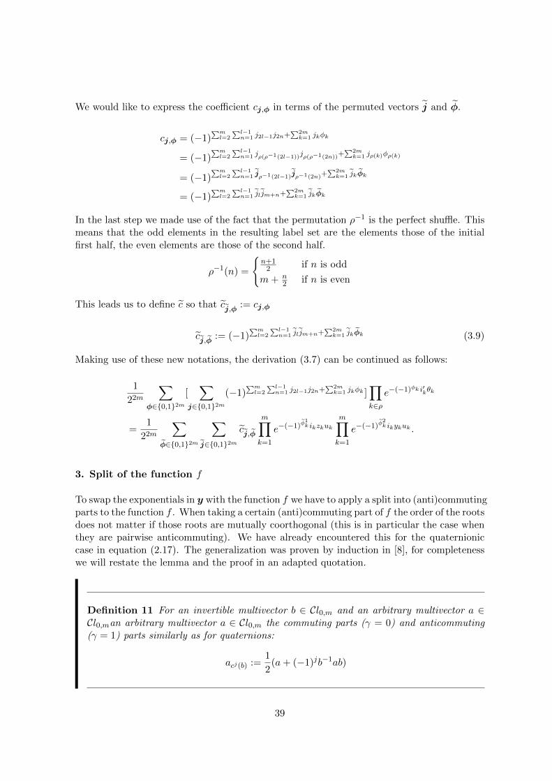
We would like to express the coefficient cj,φ in terms of the permuted vectors j and φ.

cj,φ = (−1)∑ml=2

∑l−1n=1 j2l−1j2n+

∑2mk=1 jkφk

= (−1)∑ml=2

∑l−1n=1 jρ(ρ−1(2l−1))jρ(ρ−1(2n))+

∑2mk=1 jρ(k)φρ(k)

= (−1)∑ml=2

∑l−1n=1 jρ−1(2l−1)jρ−1(2n)+

∑2mk=1 jkφk

= (−1)∑ml=2

∑l−1n=1 jljm+n+

∑2mk=1 jkφk

In the last step we made use of the fact that the permutation ρ−1 is the perfect shuffle. Thismeans that the odd elements in the resulting label set are the elements those of the initialfirst half, the even elements are those of the second half.

ρ−1(n) =

{n+12 if n is odd

m+ n2 if n is even

This leads us to define c so that cj,φ

:= cj,φ

cj,φ

:= (−1)∑ml=2

∑l−1n=1 jljm+n+

∑2mk=1 jkφk (3.9)

Making use of these new notations, the derivation (3.7) can be continued as follows:

1

22m

∑φ∈{0,1}2m

[∑

j∈{0,1}2m(−1)

∑ml=2

∑l−1n=1 j2l−1j2n+

∑2mk=1 jkφk ]

∏k∈ρ

e−(−1)φk i′kθk

=1

22m

∑φ∈{0,1}2m

∑j∈{0,1}2m

cj,φ

m∏k=1

e−(−1)φ1k ikzkuk

m∏k=1

e−(−1)φ2k ikykuk .

3. Split of the function f

To swap the exponentials in y with the function f we have to apply a split into (anti)commutingparts to the function f . When taking a certain (anti)commuting part of f the order of the rootsdoes not matter if those roots are mutually coorthogonal (this is in particular the case whenthey are pairwise anticommuting). We have already encountered this for the quaternioniccase in equation (2.17). The generalization was proven by induction in [8], for completenesswe will restate the lemma and the proof in an adapted quotation.

Definition 11 For an invertible multivector b ∈ Cl0,m and an arbitrary multivector a ∈Cl0,man arbitrary multivector a ∈ Cl0,m the commuting parts (γ = 0) and anticommuting(γ = 1) parts similarly as for quaternions:

acj(b) :=1

2(a+ (−1)jb−1ab)

39

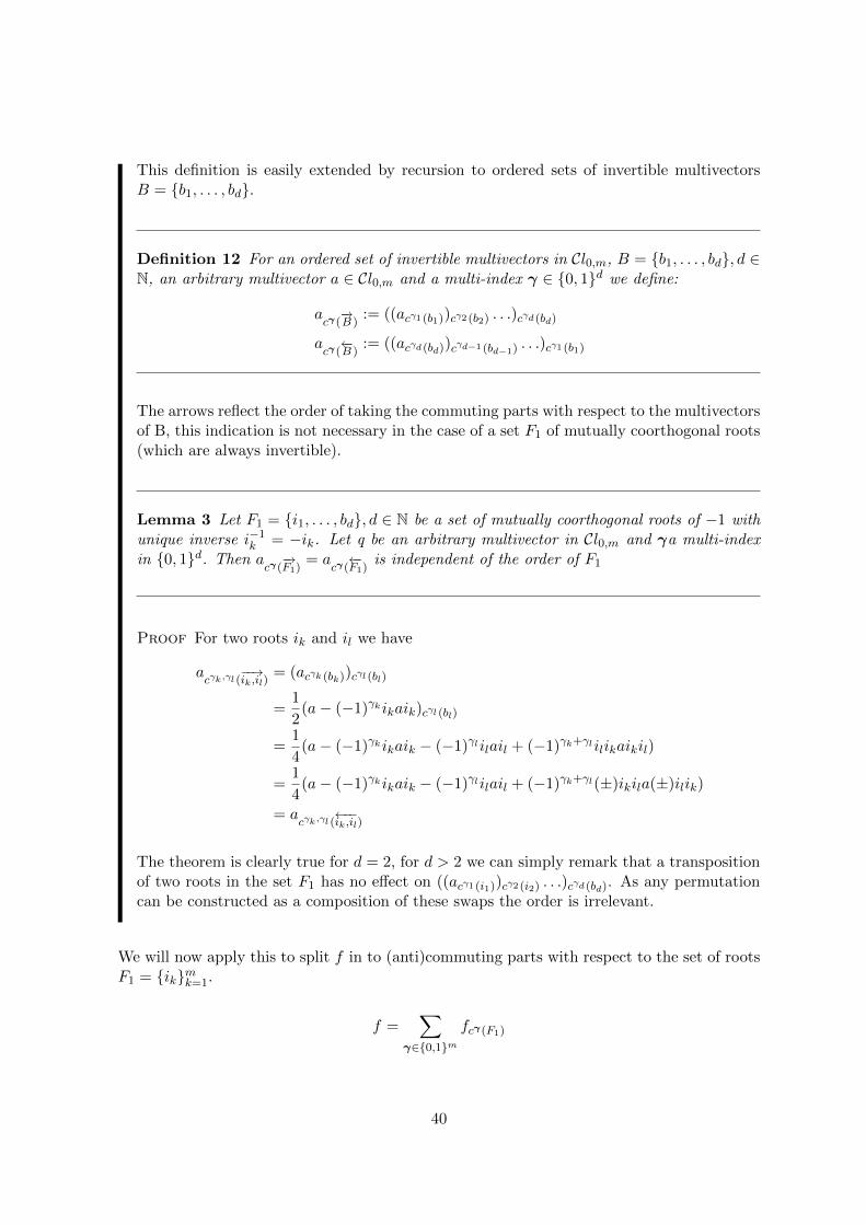
This definition is easily extended by recursion to ordered sets of invertible multivectorsB = {b1, . . . , bd}.

Definition 12 For an ordered set of invertible multivectors in Cl0,m, B = {b1, . . . , bd}, d ∈N, an arbitrary multivector a ∈ Cl0,m and a multi-index γ ∈ {0, 1}d we define:

acγ(−→B )

:= ((acγ1 (b1))cγ2 (b2) . . .)cγd (bd)

acγ(←−B )

:= ((acγd (bd))cγd−1 (bd−1). . .)cγ1 (b1)

The arrows reflect the order of taking the commuting parts with respect to the multivectorsof B, this indication is not necessary in the case of a set F1 of mutually coorthogonal roots(which are always invertible).

Lemma 3 Let F1 = {i1, . . . , bd}, d ∈ N be a set of mutually coorthogonal roots of −1 withunique inverse i−1k = −ik. Let q be an arbitrary multivector in Cl0,m and γa multi-indexin {0, 1}d. Then a

cγ(−→F1)

= acγ(←−F1)

is independent of the order of F1

Proof For two roots ik and il we have

acγk,γl (

−−→ik,il)

= (acγk (bk))cγl (bl)

=1

2(a− (−1)γkikaik)cγl (bl)

=1

4(a− (−1)γkikaik − (−1)γlilail + (−1)γk+γlilikaikil)

=1

4(a− (−1)γkikaik − (−1)γlilail + (−1)γk+γl(±)ikila(±)ilik)

= acγk,γl (

←−−ik,il)

The theorem is clearly true for d = 2, for d > 2 we can simply remark that a transpositionof two roots in the set F1 has no effect on ((acγ1 (i1))cγ2 (i2) . . .)cγd (bd). As any permutationcan be constructed as a composition of these swaps the order is irrelevant.

We will now apply this to split f in to (anti)commuting parts with respect to the set of rootsF1 = {ik}mk=1.

f =∑

γ∈{0,1}mfcγ(F1)

40

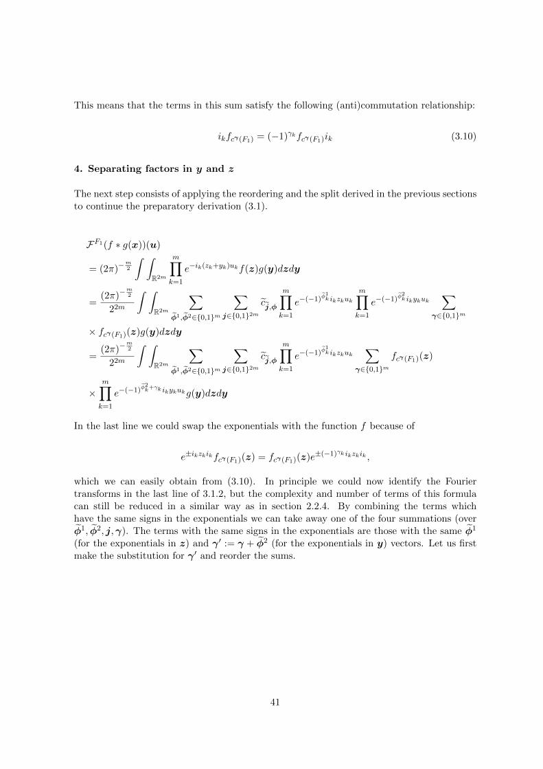
This means that the terms in this sum satisfy the following (anti)commutation relationship:

ikfcγ(F1) = (−1)γkfcγ(F1)ik (3.10)

4. Separating factors in y and z

The next step consists of applying the reordering and the split derived in the previous sectionsto continue the preparatory derivation (3.1).

FF1(f ∗ g(x))(u)

= (2π)−m2

∫ ∫R2m

m∏k=1

e−ik(zk+yk)ukf(z)g(y)dzdy

=(2π)−

m2

22m

∫ ∫R2m

∑φ1,φ2∈{0,1}m

∑j∈{0,1}2m

cj,φ

m∏k=1

e−(−1)φ1k ikzkuk

m∏k=1

e−(−1)φ2k ikykuk

∑γ∈{0,1}m

× fcγ(F1)(z)g(y)dzdy

=(2π)−

m2

22m

∫ ∫R2m

∑φ1,φ2∈{0,1}m

∑j∈{0,1}2m

cj,φ

m∏k=1

e−(−1)φ1k ikzkuk

∑γ∈{0,1}m

fcγ(F1)(z)

×m∏k=1

e−(−1)φ2k+γk ikykukg(y)dzdy

In the last line we could swap the exponentials with the function f because of

e±ikzkikfcγ(F1)(z) = fcγ(F1)(z)e±(−1)γk ikzkik ,

which we can easily obtain from (3.10). In principle we could now identify the Fouriertransforms in the last line of 3.1.2, but the complexity and number of terms of this formulacan still be reduced in a similar way as in section 2.2.4. By combining the terms whichhave the same signs in the exponentials we can take away one of the four summations (overφ1, φ2, j,γ). The terms with the same signs in the exponentials are those with the same φ1

(for the exponentials in z) and γ ′ := γ + φ2 (for the exponentials in y) vectors. Let us firstmake the substitution for γ ′ and reorder the sums.

41

FF1(f ∗ g(x))(u)

=(2π)−

m2

22m

∫ ∫R2m

∑φ1,φ2∈{0,1}m

∑j∈{0,1}2m

cj,φ

m∏k=1

e−(−1)φ1k ikzkuk

∑γ′∈{0,1}m

fcγ

′−φ2(F1)(z)

×m∏k=1

e−(−1)γ′k ikykukg(y)dzdy

=(2π)−

m2

22m

∫ ∫R2m

∑φ1∈{0,1}m

∑φ2∈{0,1}m

∑j∈{0,1}2m

cj,φ

m∏k=1

e−(−1)φ1k ikzkuk

∑γ′∈{0,1}m

fcγ

′−φ2(F1)(z)

×m∏k=1

e−(−1)γ′k ikykukg(y)dzdy

=(2π)−

m2

22m

∫ ∫R2m

∑φ1∈{0,1}m

∑γ′∈{0,1}m

∑φ2∈{0,1}m

∑j∈{0,1}2m

cj,φ

m∏k=1

e−(−1)φ1k ikzkukf

cγ′−φ2(F1)

(z)

×m∏k=1

e−(−1)γ′k ikykukg(y)dzdy

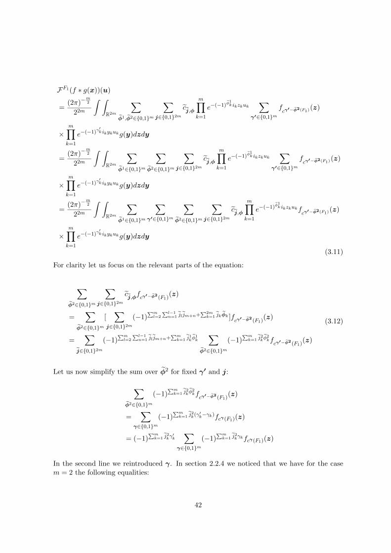
(3.11)

For clarity let us focus on the relevant parts of the equation:

∑φ2∈{0,1}m

∑j∈{0,1}2m

cj,φfcγ′−φ2 (F1)

(z)

=∑

φ2∈{0,1}m[∑

j∈{0,1}2m(−1)

∑ml=2

∑l−1n=1 jljm+n+

∑2mk=1 jkφk ]f

cγ′−φ2 (F1)(z)

=∑

j∈{0,1}2m(−1)

∑ml=2

∑l−1n=1 jljm+n+

∑mk=1 j

1kφ

1k

∑φ2∈{0,1}m

(−1)∑mk=1 j

2kφ

2kfcγ′−φ2 (F1)

(z)

(3.12)

Let us now simplify the sum over φ2 for fixed γ′ and j:

∑φ2∈{0,1}m

(−1)∑mk=1 j

2kφ

2kfcγ′−φ2 (F1)

(z)

=∑

γ∈{0,1}m(−1)

∑mk=1 j

2k(γ′k−γk)fcγ(F1)(z)

= (−1)∑mk=1 j

2kγ′k

∑γ∈{0,1}m

(−1)∑mk=1 j

2kγkfcγ(F1)(z)

In the second line we reintroduced γ. In section 2.2.4 we noticed that we have for the casem = 2 the following equalities:

42

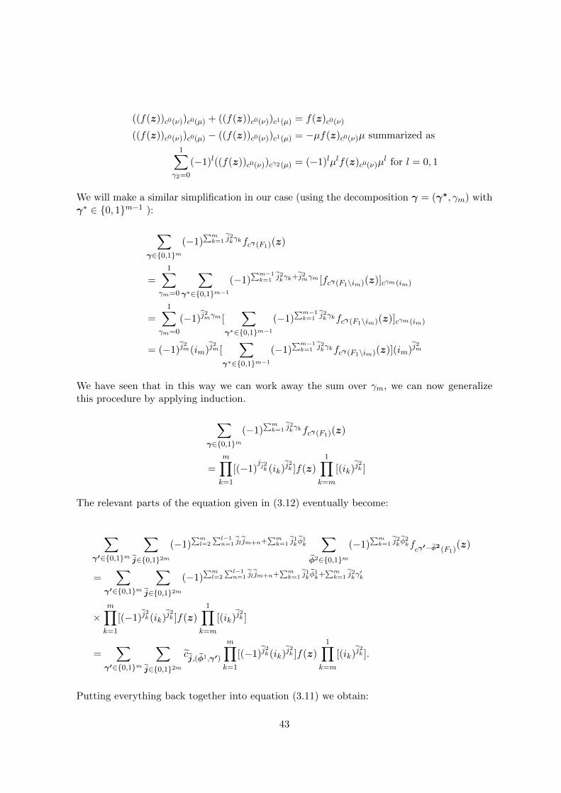
((f(z))c0(ν))c0(µ) + ((f(z))c0(ν))c1(µ) = f(z)c0(ν)

((f(z))c0(ν))c0(µ) − ((f(z))c0(ν))c1(µ) = −µf(z)c0(ν)µ summarized as

1∑γ2=0

(−1)l((f(z))c0(ν))cγ2 (µ) = (−1)lµlf(z)c0(ν)µl for l = 0, 1

We will make a similar simplification in our case (using the decomposition γ = (γ∗, γm) withγ∗ ∈ {0, 1}m−1 ):

∑γ∈{0,1}m

(−1)∑mk=1 j

2kγkfcγ(F1)(z)

=1∑

γm=0

∑γ∗∈{0,1}m−1

(−1)∑m−1k=1 j2kγk+j

2mγm [fcγ(F1\im)(z)]cγm (im)

=

1∑γm=0

(−1)j2mγm [

∑γ∗∈{0,1}m−1

(−1)∑m−1k=1 j2kγkfcγ(F1\im)(z)]cγm (im)

= (−1)j2m(im)j

2m [

∑γ∗∈{0,1}m−1

(−1)∑m−1k=1 j2kγkfcγ(F1\im)(z)](im)j

2m

We have seen that in this way we can work away the sum over γm, we can now generalizethis procedure by applying induction.

∑γ∈{0,1}m

(−1)∑mk=1 j

2kγkfcγ(F1)(z)

=m∏k=1

[(−1)jj2k (ik)

j2k ]f(z)1∏

k=m

[(ik)j2k ]

The relevant parts of the equation given in (3.12) eventually become:

∑γ′∈{0,1}m

∑j∈{0,1}2m

(−1)∑ml=2

∑l−1n=1 jljm+n+

∑mk=1 j

1kφ

1k

∑φ2∈{0,1}m

(−1)∑mk=1 j

2kφ

2kfcγ′−φ2 (F1)

(z)

=∑

γ′∈{0,1}m

∑j∈{0,1}2m

(−1)∑ml=2

∑l−1n=1 jljm+n+

∑mk=1 j

1kφ

1k+

∑mk=1 j

2kγ′k

×m∏k=1

[(−1)j2k(ik)

j2k ]f(z)

1∏k=m

[(ik)j2k ]

=∑

γ′∈{0,1}m

∑j∈{0,1}2m

cj,(φ1,γ′)

m∏k=1

[(−1)j2k(ik)

j2k ]f(z)1∏

k=m

[(ik)j2k ].

Putting everything back together into equation (3.11) we obtain:

43

FF1(f ∗ g(x))(u)

=(2π)−

m2

22m

∫ ∫R2m

∑φ1,φ2∈{0,1}m

cφ

m∏k=1

e−(−1)φ1k ikzkuk

∑γ′∈{0,1}m

fcγ′−φ1 (F1)

(z)m∏k=1

e−(−1)γ′k ikykukg(y)dzdy

=(2π)−

m2

22m

∑φ1,γ′∈{0,1}m

∑j∈{0,1}2m

cj,(φ1,γ′)

∫ ∫R2m

m∏k=1

e−(−1)φ1k ikzkuk

m∏k=1

[(−1)j2k(ik)

j2k ]f(z)

×1∏

k=m

[(ik)j2k ]

m∏k=1

e−(−1)γ′k ikykukg(y)dzdy.

Here we will choose to factor in the second product of roots in the GFT of g, that is why they

still need to be swapped with∏mk=1 e

−(−1)γ′k ikykuk . Every root that passes an exponential

with a different root changes the sign of the exponential. Using the notation J2 :=∑m

k=1 j2k

we get

m∏k=1

[(ik)j2k ]

m∏k=1

e−(−1)γ′k ikykuk =

m∏k=1

e−(−1)γ′k+J

2−j2k ikykuk

m∏k=1

[(ik)j2k ]. (3.13)

Remark that the sums in the powers of −1 and the changes of sign satisfy modulo 2 arithmetic,we will use this frequently in the manipulations below.

With this minor modification the formula becomes:

FF1(f ∗ g(x))(u)

=(2π)−

m2

22m

∑φ1,γ′∈{0,1}m

∑j∈{0,1}2m

cj,(φ1,γ′)

∫ ∫R2m

m∏k=1

e−(−1)φ1k ikzkuk

m∏k=1

[(−1)j2k(ik)

j2k ]f(z)

×m∏k=1

e−(−1)γ′k+J

2+j2k ikykuk

1∏k=m

[(ik)j2k ]g(y)dzdy.

5. Identification of the geometric Fourier transforms

The number of terms in the formula can still be reduced, the sum over j1 will also simplifyand yield a factor 2m. To make the notation a bit lighter we will first identify the transforms.

44

FF1(f ∗ g(x))(u)

=(2π)−

m2

22m

∑φ1,γ′∈{0,1}m

∑j∈{0,1}2m

cj,(φ1,γ′)

∫Rm

m∏k=1

e−(−1)φ1k ikzkuk

m∏k=1

[(−1)j2k(ik)

j2k ]f(z)dz

×∫Rm

m∏k=1

e−(−1)γ′k+J

2−j2k ikykuk

1∏k=m

[(ik)j2k ]g(y)dy

=(2π)

m2

22m

∑φ1,γ′∈{0,1}m

∑j∈{0,1}2m

cj,(φ1,γ′)

FF1(m∏k=1

[(−1)j2k(ik)

j2k ]f φ1(z))FF1(

1∏k=m

[(ik)j2k ]gγ

′+J2−j2(y))

In the last line J2 has to be treated as a vector with m components J2. We can subsequentlytake the inverse transform and use the definition of the Mustard convolution.

f ∗g =1

22m

∑φ1,γ′∈{0,1}m

∑j∈{0,1}2m

cj,(φ1,γ′)

m∏k=1

[(−1)j2k(ik)

j2k ]f φ1∗F1

1∏k=m

[(ik)j2k ]gγ

′+J2−j2 (3.14)

6. Further reduction

Notice that the sums over φ1,γ′ and j2 are essential, they characterize the different termsin the convolution. The sum over j1 can still be reduced for fixed values of φ1,γ′ and j2.The sum of the coefficients for these fixed values in equation (3.14) can be simplified by using∑1

a=0(−1)ab = 2δ0,b.

∑j1∈{0,1}m

cj,(φ1,γ′)

m∏k=1

(−1)j2k

=∑

j1∈{0,1}m(−1)

∑ml=2

∑l−1n=1 j

1l j

2n+

∑mk=1 j

1kφ

1k+

∑mk=1 j

2kγ′k+

∑mk=1 j

2k

=∑

j1∈{0,1}m(−1)j

11 φ

11+

∑ml=2 j

1l [∑l−1n=1 j

2n+φ

1l ]+

∑mk=1 j

2k[γ′k+1]

= 2mδ0,φ11

m∏l=2

[δ0,∑l−1n=1 j

2n+φ

1l](−1)

∑mk=1 j

2k[γ′k+1]

(3.15)

The coupling between the summed vector j1 and the vectors φ1, j2 induces restrictions onthe values of φ1 and j2.

{φ11 = 0

φ1l =∑l−1

n=1 j2n l ∈ {2, . . . ,m}

(3.16)

45

The goal is now to use these restrictions to work away the sum over φ1 in equation (3.14).To clean up the equation we also introduce some new notations:

β :=γ′ + J2 + j2

t :=j2

These definitions give as consequence:

γ′ = β + J2 + j2.

With these new notations and restrictions we can rewrite the prefactor in (3.15) (using modulo2 arithmetic).

m∑k=1

j2k [γ′k + 1]2=

m∑k=1

j2k(βk + J2 + j2k + 1)

2=

m∑k=1

j2k(βk + 1) + J2J2 +m∑k=1

j2k j2k using a2

2= a

2=

m∑k=1

j2k(βk + 1) + J2 +m∑k=1

j2k

2=

m∑k=1

j2k(βk + 1)

2=

m∑k=1

tk(βk + 1)

(3.17)

In this way we obtain a reduced convolution formula from the version in equation (3.14).

f ∗ g

=1

22m

∑φ1,γ′∈{0,1}m

∑j∈{0,1}2m

cj,(φ1,γ′)

m∏k=1

[(−1)j2k(ik)

j2k ]f φ1 ∗F1

1∏k=m

[(ik)j2k ]gγ

′+J2−j2

=1

2m

∑t∈{0,1}m

∑β∈{0,1}m

(−1)∑mk=1 tk(βk+1)

m∏k=1

[(ik)tk ]f (0,t1,t1+t2,...,

∑l−1n=1 tn,...) ∗F1

1∏k=m

[(ik)tk ]gβ

=1

2m

∑t∈{0,1}m

∑β∈{0,1}m

dβ,t

m∏k=1

[(ik)tk ]f (0,t1,t1+t2,...,

∑l−1n=1 tn,...) ∗F1

1∏k=m

[(ik)tk ]gβ

If we solve the system (3.16) for j2 (modulo 2) then we obtain the solved system (3.18) below.

{φ11 = 0

j2n =∑n+1

l=2 φ1l n ∈ {1, . . . ,m− 1}

(3.18)

46

We write the restrictions in this form so we can work away the sum over j2 instead of thesum over φ1. In this way the sum over the sign changes of f remain clear. Notice thatj2m = tm is unrestricted. We now introduce also a clean replacement of α := (φ1k)

mk=2 (where

αisin{0, 1}m−1) of the vector φ1 ( φ11 = 0). By introducing α the prefactor (3.17) becomes.

m∑k=1

j2k [γ′k + 1]2=

m∑k=1

j2k(βk + 1)

2=

m−1∑k=1

(k+1∑l=2

φ1l )(βk + 1) + tm(βm + 1)

2=

m−1∑k=1

(

k∑l=1

αl)(βk + 1) + tm(βm + 1).

Plugging the second set of restrictions (3.18) and new notations gradually into equation (3.14)we can derive our final result.

f ∗ g

=1

22m

∑φ1,γ′∈{0,1}m

∑j∈{0,1}2m

cj,(φ1,γ′)

m∏k=1

[(−1)j2k(ik)

j2k ]f φ1 ∗F1

1∏k=m

[(ik)j2k ]gγ

′+J2−j2

=1

22m

1∑φ11=0

∑α∈{0,1}m−1

∑γ′,j1,j2∈{0,1}m

cj,(φ1,γ′)

m∏k=1

[(−1)j2k(ik)

j2k ]f φ1 ∗F1

1∏k=m

[(ik)j2k ]gγ

′+J2−j2

=1

2m

∑α∈{0,1}m−1

∑β∈{0,1}m

1∑tm=0

(−1)∑m−1k=1 (

∑kl=1 αl)(βk+1)+tm(βm+1)

m−1∏k=1

[(ik)∑kl=1 αl ](im)tm

× f (0,α) ∗F1 (im)tm1∏

k=m−1[(ik)

∑kl=1 αl ]gβ

=1

2m

∑α∈{0,1}m−1

∑β∈{0,1}m

1∑tm=0

eα,β,tm

m−1∏k=1

[(ik)∑kl=1 αl ](im)tmf (0,α) ∗F1 (im)tm

1∏k=m−1

[(ik)∑kl=1 αl ]gβ

In the last line we defined the coefficients eα,β,tm . We can summarize this rather long deriva-tion in the main theorem of this part.

47

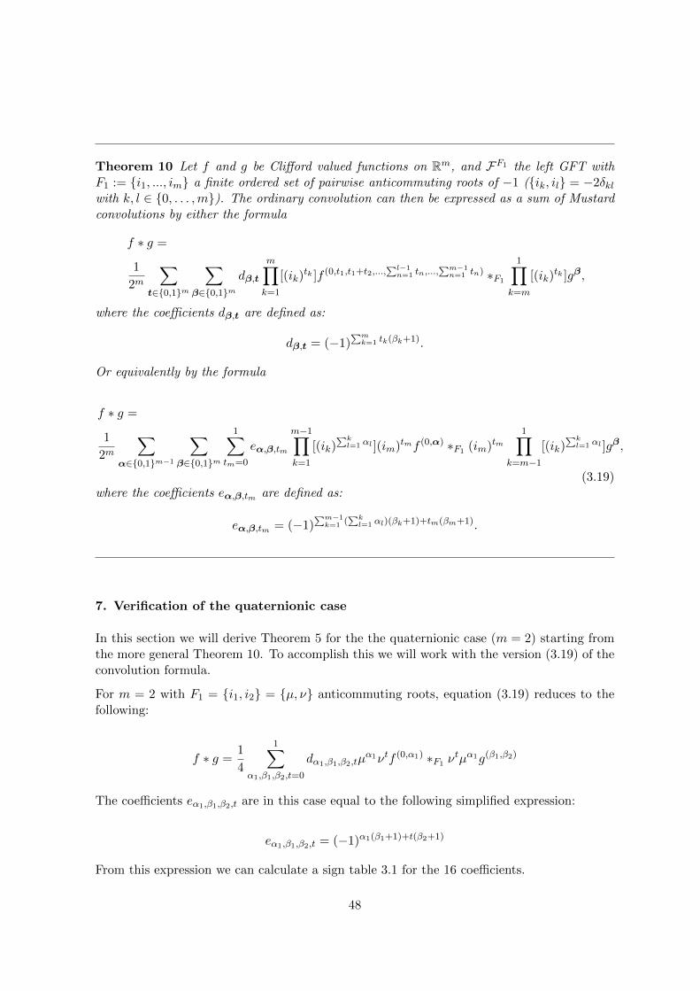
Theorem 10 Let f and g be Clifford valued functions on Rm, and FF1 the left GFT withF1 := {i1, ..., im} a finite ordered set of pairwise anticommuting roots of −1 ({ik, il} = −2δklwith k, l ∈ {0, . . . ,m}). The ordinary convolution can then be expressed as a sum of Mustardconvolutions by either the formula

f ∗ g =

1

2m

∑t∈{0,1}m

∑β∈{0,1}m

dβ,t

m∏k=1

[(ik)tk ]f (0,t1,t1+t2,...,

∑l−1n=1 tn,...,

∑m−1n=1 tn) ∗F1

1∏k=m

[(ik)tk ]gβ,

where the coefficients dβ,t are defined as:

dβ,t = (−1)∑mk=1 tk(βk+1).

Or equivalently by the formula

f ∗ g =

1

2m

∑α∈{0,1}m−1

∑β∈{0,1}m

1∑tm=0

eα,β,tm

m−1∏k=1

[(ik)∑kl=1 αl ](im)tmf (0,α) ∗F1 (im)tm

1∏k=m−1

[(ik)∑kl=1 αl ]gβ,

(3.19)where the coefficients eα,β,tm are defined as:

eα,β,tm = (−1)∑m−1k=1 (

∑kl=1 αl)(βk+1)+tm(βm+1).

7. Verification of the quaternionic case

In this section we will derive Theorem 5 for the the quaternionic case (m = 2) starting fromthe more general Theorem 10. To accomplish this we will work with the version (3.19) of theconvolution formula.

For m = 2 with F1 = {i1, i2} = {µ, ν} anticommuting roots, equation (3.19) reduces to thefollowing:

f ∗ g =1

4

1∑α1,β1,β2,t=0

dα1,β1,β2,tµα1νtf (0,α1) ∗F1 ν

tµα1g(β1,β2)

The coefficients eα1,β1,β2,t are in this case equal to the following simplified expression:

eα1,β1,β2,t = (−1)α1(β1+1)+t(β2+1)

From this expression we can calculate a sign table 3.1 for the 16 coefficients.

48

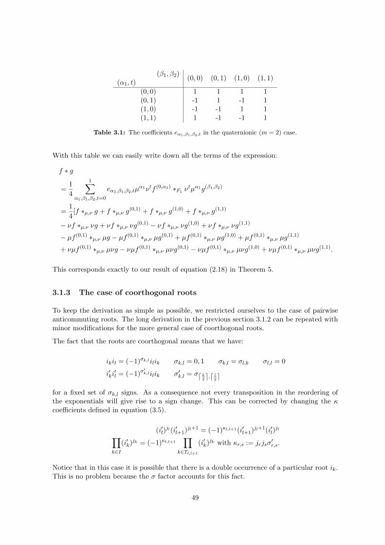
(α1, t)(β1, β2) (0, 0) (0, 1) (1, 0) (1, 1)

(0, 0) 1 1 1 1(0, 1) -1 1 -1 1(1, 0) -1 -1 1 1(1, 1) 1 -1 -1 1

Table 3.1: The coefficients eα1,β1,β2,t in the quaternionic (m = 2) case.

With this table we can easily write down all the terms of the expression:

f ∗ g

=1

4

1∑α1,β1,β2,t=0

eα1,β1,β2,tµα1νtf (0,α1) ∗F1 ν

tµα1g(β1,β2)

=1

4[f ∗µ,ν g + f ∗µ,ν g(0,1) + f ∗µ,ν g(1,0) + f ∗µ,ν g(1,1)

− νf ∗µ,ν νg + νf ∗µ,ν νg(0,1) − νf ∗µ,ν νg(1,0) + νf ∗µ,ν νg(1,1)

− µf (0,1) ∗µ,ν µg − µf (0,1) ∗µ,ν µg(0,1) + µf (0,1) ∗µ,ν µg(1,0) + µf (0,1) ∗µ,ν µg(1,1)

+ νµf (0,1) ∗µ,ν µνg − νµf (0,1) ∗µ,ν µνg(0,1) − νµf (0,1) ∗µ,ν µνg(1,0) + νµf (0,1) ∗µ,ν µνg(1,1).

This corresponds exactly to our result of equation (2.18) in Theorem 5.

3.1.3 The case of coorthogonal roots

To keep the derivation as simple as possible, we restricted ourselves to the case of pairwiseanticommuting roots. The long derivation in the previous section 3.1.2 can be repeated withminor modifications for the more general case of coorthogonal roots.

The fact that the roots are coorthogonal means that we have:

ikil = (−1)σk,lilik σk,l = 0, 1 σk,l = σl,k σl,l = 0

i′ki′l = (−1)σ

′k,lilik σ′k,l = σd k2e,d l2e

for a fixed set of σk,l signs. As a consequence not every transposition in the reordering ofthe exponentials will give rise to a sign change. This can be corrected by changing the κcoefficients defined in equation (3.5).

(i′l)jl(i′l+1)

jl+1 = (−1)κl,l+1(i′l+1)jl+1(i′l)

jl∏k∈I

(i′k)jk = (−1)κl,l+1

∏k∈Tl,l+1

(i′k)jk with κr,s := jrjsσ

′r,s.

Notice that in this case it is possible that there is a double occurrence of a particular root ik.This is no problem because the σ factor accounts for this fact.

49

The c coefficient (see equations (3.8) and (3.9) ) needs to be adjusted accordingly:

cj,φ

:= (−1)∑ml=2

∑l−1n=1 jljm+nσ′2l−1,2n+

∑2mk=1 jkφk

:= (−1)∑ml=2

∑l−1n=1 jljm+nσl,n+

∑2mk=1 jkφk

Another step where the swapping of roots comes into play is the minor modification describedby equation (3.13). The goal of this equation was to bring the factors inside the GFT of g.

Every root (ik)j2k that passes an exponential in a certain root il will now change the sign of

the exponential by a factor (−1)j2kσk,l . Using the renewed notation J2

l :=∑m

k=1 j2kσk,l we get:

m∏k=1

[(ik)j2k ]

m∏k=1

e−(−1)γ′k ikykuk =

m∏k=1

e−(−1)γ′k+J

2k−j

2k ikykuk

m∏k=1

[(ik)j2k ].

There are no further steps where we need to swap roots in the derivation,this means thatequation (3.14) can be easily adapted to this more general case with the new c coefficientsand changes of sign in g.

f ∗ g =1

22m

∑φ1,γ′∈{0,1}m

∑j∈{0,1}2m

cj,(φ1,γ′)

m∏k=1

[(−1)j2k(ik)

j2k ]f φ1 ∗F1

1∏k=m

[(ik)j2k ]gγ

′+J2

In this equation J2 needs to be interpreted as the vector with components J2l .

To accomplish the further reduction we still need a minor adaptation in equation (3.15).

∑j1∈{0,1}m

cj,(φ1,γ′)

m∏k=1

(−1)j2k

=∑

j1∈{0,1}m(−1)

∑ml=2

∑l−1n=1 j

1l j

2nσl,n+

∑mk=1 j

1kφ

1k+

∑mk=1 j

2kγ′k+

∑mk=1 j

2k

= 2mδ0,φ11

m∏l=2

[δ0,∑l−1n=1 j

2nσl,n+φ

1l](−1)

∑mk=1 j

2k[γ′k+1]

Leading to a different set of restrictions.

{φ11 = 0

φ1l =∑l−1

n=1 j2nσl,n l ∈ {2, . . . ,m}

This system is not solved as easily in the previous case because of all the different possibilitiesfor σl,n, that is why we will stick with the first formulation of the theorem. The substitutionof a new β defined by

50

β :=γ′ + J2

γ′ =β + J2

leads to the same result for the prefactor in (3.15). This is again easily proved using modulo2 arithmetic.

m∑k=1

j2k [γ′k + 1]2=

m∑k=1

j2k(βk + J2k + 1)

2=

m∑k=1

j2k(βk + 1) +

m∑k=1

m∑l=1

j2k j2l σk,l using σk,l = σl,k, σl,l = 0

2=

m∑k=1

j2k(βk + 1) + 2

m∑k=1

∑l<k

j2k j2l σk,l

2=

m∑k=1

tk(βk + 1)

Introducing all these minor adaptations in to the result of Theorem 10 we can derive the moregeneral theorem stated below.

Theorem 11 Let f and g be Clifford valued functions on Rm, and FF1 the left GFT withF1 := {i1, ..., im} a finite ordered set of ‘coorthogonal’ roots of −1 such that ikil = (−1)σk,lilik.The ordinary convolution can then be expressed as a sum of Mustard convolutions by thefollowing formula:

f ∗ g

=1

2m

∑t∈{0,1}m

∑β∈{0,1}m

dβ,t

m∏k=1

[(ik)tk ]f (0,t1σ2,1,...,

∑l−1n=1 tnσl,n,...) ∗F1

1∏k=m

[(ik)tk ]gβ

Where the coefficients dβ,t are defined as:

dβ,t = (−1)∑mk=1 tk(βk+1).

51

3.2 Outlook and conclusions

To conclude part I we will look back upon the formulas that are derived. Let us recall themain objective.

ObjectiveFind term dependent Clifford numbers a, b, c ∈ Cl0,m such that the ordinary convolutioncan be expressed as a finite linear combination of Mustard convolutions:

(f ∗ g)(x) =∑φ,γ

aφ,γfφ ∗F1,F2 bφ,γg

γcφ,γ .

We clearly succeeded to obtain such a formula in several cases. The quaternionic case m = 2is solved in all situations. In the Clifford algebraic case we derived the formula in the mostimportant cases.

In doing so we did not only prove an explicit formula but also guaranteed its existence andthe fact that it has a finite number of terms. On the other hand it is clear that theseformulas are not unique. Swapping the roots with the transforms, the functions and witheach other would lead to equivalent formulas. The most general case of square roots of −1in a Clifford algebra eluded us for a very good reason. The matters for this case quicklybecome complicated because for two general Clifford numbers a and b it is not guaranteedthat either their commutator or anticommutator is real. One can in fact construct a simplecounterexample in Cl0,3 that disproves this:

{e1e2 + e2e3, e1} = e1e2e1 − e1e1e2 + e2e3e1 − e1e2e3 = 2e2

[e1e2 + e2e3, e1] = e1e2e1 + e1e1e2 + e2e3e1 + e1e2e3 = 2e1e2e3

We can easily normalize the Clifford number e1e2 + e2e3 so that we obtain a root of −1:( e1e2+e2e3√

2)2 = −1. This makes the swapping of the roots needed in the reordering much more

complicated. A very speculative possible method is explained below. It seems plausible thatthe roots will have to be expanded in a basis of the Clifford algebra (e1, e2, . . . , em) where thebasisfunctions are coorthogonal by definition. Multiplying out all exponentials as productsof sines, cosines and these coorthogonal basisfunctions can give us a chance at reorderingthese exponentials with the general approach applied in the previous section. This is ill-advised because the complexity and cumbersomeness of the calculations would not outweighthe benefits of having an explicit formula in this case.

The techniques and the procedures above might be applied to other Clifford algebraic Fouriertransforms and convolutions. And by this not only the right GFT and others are meant, butalso more general Fourier transforms that are based on a kernel with exponentials of Cliffordnumbers. If one would be still interested in this topic from a purely mathematical point ofview there are still some open questions to be answered. First of all, why are the coefficientsin the forward and the reverse formula the same in the quaternionic anticommuting case?

52

Can this be proven by an indirect but shorter way? Second does this symmetry still hold inthe Clifford algebraic setting? The latter is now obscured by the fact that the expressions forthe coefficients are not easily compared in both formulas.

It seems that the real benefit of these formulas and techniques will come from applicationsin data and signal processing. These applications will in first instance be limited to thequaternionic case. That is why we will now turn our focus on these applications in part 2.

53

Part II

Applications of quaternionicconvolution formulas

54

Chapter 4

Quaternions in image processing

Nowadays hypercomplex numbers have many applications in data analysis, signal and imageprocessing. They provide an important alternative to ‘classical’ data manipulations whichwork with vectors in Rn. For quaternions in particular the applications are mostly situatedwithin the field of image processing. There are some interesting developments in this newfield of image processing. Quaternions have been used to obtain saliency maps in [1] and[2], for disparity estimation in [18], for pattern recognition in [23], etc.. . There are alsogeneralizations of wavelet transforms (see for example [26] or [3],[4]).

In part I we derived convolution formulas in a hypercomplex setting. These formulas arealready interesting from a pure mathematical viewpoint, but in this part we take the develop-ment of these formulas a step further by discretizing them and applying them to images. Theobjective is to get a better understanding of the quaternionic spectrum of images and filterdesign by the application of these formulas. To that end we will work with a quaternioniccolor edge filter designed by S. Sangwine ([25], [15]). This detection method will serve as atoy model to develop a better understanding of the spectral domain. The working principlesof the detector will be explained in this chapter, the background information required for thisis provided in chapter 4.

In image processing many manipulations are based on marginal methods. This means thatthe three color channels composing the image (for example RGB: Red, Green and Blue, moredetail in the next section 4.1) are processed separately. Although the computational efficiencyand the relative ease of implementation are some strong advantages of these methods, theyoften perform poorly due to the lack of spectral color information and they do not allowto detect color discontinuities ([22],[20]). To circumvent these disadvantages, images canalso be processed with vectorial methods ([21],[22]). The pixels are treated as vectors inR3, usually representing some color space like RGB, XYZ or Luv. These vector filteringmethods have many applications in image processing and signal analysis, but they lack anunderlying theoretical framework. As a consequence the development of these methods arerather ad-hoc. The use of quaternions (which are a special case of hypercomplex numbers)promises a solution in this respect. The geometric interpretations of the quaternion algebraallow for the understanding of algebraic manipulations as rotations, dilations and other affinetransformations in 3-space. This gives us a clear intuitive picture of the filters and theirdesign. After some background on color spaces, we will explain quaternionic pixels.

55

4.1 Images and color spaces

Images and color spaces or of such importance that this section is common knowledge, and wetry to limit ourselves to explain what is needed to understand the rest of the thesis. Interestedreaders who want a more thorough discussion can find a more detailed exposition about colorspaces in the book of Fairchild [16].

4.1.1 The LMS color space

Light is the part of the continuous spectrum of electromagnetic waves which is observable tohumans. The human eye is a complicated piece of biology but it only has 3 different typesof chromatic sensitive photo receptors called cones. A certain spectrum gets interpreted bya complex neurophysiological process which occurs partly in the brain and partly in theretina. Each continuous spectrum which is in a certain sense in an infinite dimensionalspace gets reduced - or in more mathematical terms, projected - by our perception to a 3dimensional space. Each color can thus be characterized by three numbers. This leads tothe fact that two totally different spectra can be perceived as the same color by us. Thisperception is off course different for every person, but with the advent of television there wasa need for standardization. With a series of experiments the CIE (International Commisionon Illumination) established the standard sensitivity curves which depict the absorption forall frequencies. It appears to be that one type of cones is responsible for the long wavelengthsensitivity (L 560-580 nm), another for the mid range (M 530-540 nm) and a third type forthe short range (S 420-440 nm). Weighting a certain power spectrum with these 3 functionsgives rise to 3 objective values L, M and S. These are the so called tristimulus values of theLMS color space.

4.1.2 The RGB color space

It is obvious that there is no such thing as negative intensity, as a result certain combinationsof tristimulus values which can only be obtained with a negative power spectrum will notrepresent a color. This is in fact the case for the three primaries (the standard basis of thecolor space {(0, 0, 1), (0, 1, 0), (1, 0, 0)}) of the LMS-space. This is a serious problem whendoing color matching experiments, where the three primaries are added to match a certainmonochromatic color (one spectral line). By making the (remarkably precise) observation ofGrassmann that colors are additive, one can then know the 3 values of any color spectrumby integrating over the values of the monochromatic values (the color matching functions).Historically these where actually the first experiments that were executed (1931). The 3primaries which were chosen, were perceived to respectively have a red, green and blue hue.They were based on the spectral lines of phosphor (because of its use in CRT screens). Thisgave rise to the first mathematically defined colorspace called the CIE RGB 1931 color space.

Due to the fact these spaces are three dimensional and their relationship is linear, the valuesof a certain color in the different spaces are linked by a 3 × 3 transformation matrix. TheRGB values are normalized so the values lie between 0 and 255 or between 0 and 1. As a

56

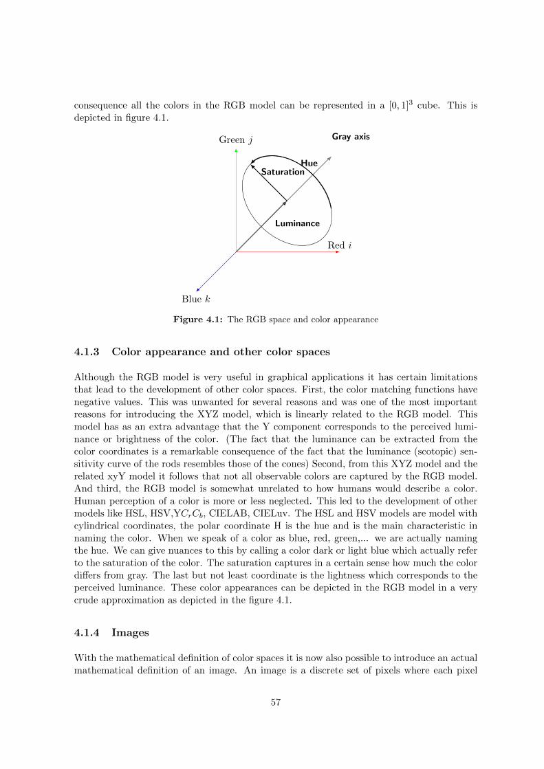
consequence all the colors in the RGB model can be represented in a [0, 1]3 cube. This isdepicted in figure 4.1.

Luminance

SaturationHue

Gray axis

Red i

Green j

Blue k

Figure 4.1: The RGB space and color appearance

4.1.3 Color appearance and other color spaces

Although the RGB model is very useful in graphical applications it has certain limitationsthat lead to the development of other color spaces. First, the color matching functions havenegative values. This was unwanted for several reasons and was one of the most importantreasons for introducing the XYZ model, which is linearly related to the RGB model. Thismodel has as an extra advantage that the Y component corresponds to the perceived lumi-nance or brightness of the color. (The fact that the luminance can be extracted from thecolor coordinates is a remarkable consequence of the fact that the luminance (scotopic) sen-sitivity curve of the rods resembles those of the cones) Second, from this XYZ model and therelated xyY model it follows that not all observable colors are captured by the RGB model.And third, the RGB model is somewhat unrelated to how humans would describe a color.Human perception of a color is more or less neglected. This led to the development of othermodels like HSL, HSV,YCrCb, CIELAB, CIELuv. The HSL and HSV models are model withcylindrical coordinates, the polar coordinate H is the hue and is the main characteristic innaming the color. When we speak of a color as blue, red, green,... we are actually namingthe hue. We can give nuances to this by calling a color dark or light blue which actually referto the saturation of the color. The saturation captures in a certain sense how much the colordiffers from gray. The last but not least coordinate is the lightness which corresponds to theperceived luminance. These color appearances can be depicted in the RGB model in a verycrude approximation as depicted in the figure 4.1.

4.1.4 Images

With the mathematical definition of color spaces it is now also possible to introduce an actualmathematical definition of an image. An image is a discrete set of pixels where each pixel

57

represents a color. We can make this more formal by defining an image as a map.

Definition 13 An image with respect to a certain color space (we will restrict ourselves toRGB) in R3 and a certain size (N,M) is a map from {1, N} × {1,M} to this color space ,i.e.:

ψ : {1, N} × {1,M} 7→ R3 (i, j) 7→ (R(i, j), G(i, j), B(i, j))

In this thesis we will always work with the RGB model. However, it is immediately e possibleto expand the methods below to other color spaces.

4.2 Quaternionic pixels

In this section we will briefly explain how we can encode the information of our color spacesinto quaternions. The construction is made by a map from the color space to the purequaternions.

Definition 14 Let the numbers in R3 represent some color space. Then we can associatewith each pixel a quaternionic pixel by the following map:

φ : R3 7→ Cl0,2 (R,G,B) 7→ Ri+Gj +Bk

This map is applied pixelwise on the whole image, this means that a quaternionic image willsimply be the composition of ψ and φ.

4.2.1 Quaternions and rotations in color space

The quaternionic pixels will allow us to give a theoretical framework underpinning the ideasin filter design. Quaternions make geometric transformations such as reflections and rotationseasy. The special relation between quaternions and rotations is not exclusive for quaternions.In chapter 1 of part I we introduced the definitions of Clifford algebras and in particular wecould identify the quaternions H as the Clifford algebra Cl0,2. Clifford algebras are closelyrelated to the orthogonal O(n) and special orthogonal SO(n) transformation groups. They

58

allow in fact the construction of the Pin(n) and Spin(n) groups, defined as:

Pin(n) =

k∏j=1

ωj |ωj ∈ Sn−1

Spin(n) =

2k∏j=1

ωj |ωj ∈ Sn−1 .

These groups have the same Lie algebra as respectively O(n) and SO(n), and are in factdouble covers of these Lie groups. Without going into to much detail, we will make this moreexplicit for the case of the quaternions H ∼= Cl0,2.

Consider a unit quaternion q, i.e. a quaternion with |q|2 = qq = 1. Then we can always findan axis κ2 = −1 such that we can write q as

q = exp

(θ

2κ

)= cos

(θ

2

)+ sin

(θ

2

)κ.

As we will see, the unit quaternions can in fact be viewed as parameterizations of rotationsin R3. They are used so often in applications involving rotations in 3D that they have theirown name. They are called versors. The group of all these versors is isomorphic to Sp(1).Without proof we state here that it is in fact isomorphic to Spin(3) and SU(2). (See forexample [19]) The fact that SU(2) is a double cover of SO(3) is well know to physicists: itdefines the transformation of the spin of spin 1/2 particles under SO(3).

We can now consider the conjugation action of such a versor q on an vector r of R3, whereR3 is embedded into the quaternions by φ defined in definition 14.

r′ = qrq−1

= (cosθ

2+ κ sin

θ

2)r(cos

θ

2− κ sin

θ

2)

= r cos2θ

2+ (κr − rκ) sin

θ

2cos

θ

2− κrκ sin2 θ

2

We can use expression (1.3) to reduce this even further.

r′ = r cos2θ

2+ 2(κ× r) sin

θ

2cos

θ

2− (r(κ · κ)− 2κ(κ · r)) sin2 θ

2

= r(cos2θ

2− sin2 θ

2) + (κ× r)(2 sin

θ

2cos

θ

2) + κ(κ · r)(2 sin2 θ

2)

= r cos θ + (κ× r) sin θ + κ(κ · r)(1− cos θ)

= (r − κ(κ · r)) cos θ + (κ× r) sin θ + κ(κ · r)= r⊥ cos θ + (κ× r⊥) sin θ + r‖,

where r⊥ is the orthogonal projection of r on k and r‖ is the parallel projection of r onk. We see that the conjugation action of q on r accomplishes a rotation of the vector r

59

over an angle θ around the axis of rotation κ. The group of versors is a double cover ofSO(3), which can simply be observed by noting that −q gives rise to the same rotationr′ = (−q)r(−q)−1 = qrq−1. In our case we will often choose the axis of rotation κ to be thegray axis µ.

60

Chapter 5

Color edge filtering by usingquaternions

Now the basics of quaternionic image processing are explained, the color edge filter of Sang-wine (originally introduced in [25]) can be studied. In section 5.1 the filter is introduced in thespatial domain, where it was orginally designed. Afterwards in section 5.2 the spectrum willbe constructed and studied. The study of the spectrum requires the introduction of discreteversions of the QFT, the convolutions and the convolution formulas derived in part I. Thesebasic tools will be derived along the way.

5.1 The color edge detector in the spatial domain

As explained in the previous chapter 4 an image is a map from a two-dimensional set {0,M −1} × {0, N − 1} to some color space or in our case the pure quaternions. Applying a filteron the image is done by convolving the image f with one or two masks (hL, hR). The sizeof the masks will be denoted as (Mm, Nm). We have to introduce the discrete quaternionicconvolution products to accomplish the filtering.

5.1.1 Discrete quaternionic convolutions

The noncommutativity of the quaternions leads to the fact that there are 3 convolutionproducts. (see for example [15])

61

Definition 15 The discrete left and right quaternionic convolutions are respectivelydefined as:

hL ∗ f(m,n) =M−1∑i=0

N−1∑j=0

hL(i, j)f(m− i, n− j)

f ∗ hR(m,n) =M−1∑i=0

N−1∑j=0

f(m− i, n− j)hR(i, j).

The quaternionic biconvolution is defined as:

hL ≺ f � hR(m,n) =M−1∑i=0

N−1∑j=0

hL(i, j)f(m− i, n− j)hR(i, j).

We have to make some extra remarks concerning these definitions.

First of all we have to take care of the boundaries of the image. When the mask is convolvedwith the pixels on the boundary some parts of the mask will fall outside the limits of theimage. To solve this minor problem we can impose boundary conditions or we can make useof zero padding. Here periodic boundary conditions will be used. This means that the imagef will be periodically extended:

f(x1 + iN, x2 + jN) = f(x1, x2) i, j ∈ Z with 0 ≤ x1 ≤M − 1 and 0 ≤ x2 ≤ N − 1.

We have chosen this because it is the mathematically elegant solution. The main disadvantageis of course that it connects pixels from far away areas. When the mask is small comparedto the image (Mn � M,Nn � N), the result will only be different in a small strip near theboundaries and is irrelevant.

Second, the set of possible masks that are to be used in a filter are restricted because theresult of the convolution has to be a pure quaternion. This is a fact to be reckoned with whendesigning a filter. Third, we see that the right and left convolutions accomplish the same, ifthe interpretation of the image f and the mask h is swapped.

Finally it seems that the continuous convolution formulas from part I do not apply to thebiconvolution. Luckily this biconvolution can be rewritten as a sum of right or left convolu-tions if we apply a split to the corresponding mask and the image. The purpose of the splitis to allow the commutation of components of the mask with the components of the image.

The subsequent calculation is adapted from the paper [15]. We split the mask in 3 axiallyinvariant components with respect to the basis of the pure quaternions formed by the gray axisµ (µ1 = µ = i+j+k√

3), an axis chosen orthogonal to µ (µ2 = ν) and their product (µ3 = µν).

They form an orthonormal basis of the pure quaternions: {µi, µj} = −2δij . Performing thissplit yields

62

hL = h1 + h2 + h3

h1 = h′0 + h′1µ1 h′0, h′1 ∈ R

h2 = h′2µ2 h′2 ∈ Rh3 = h′3µ3 h′3 ∈ R

Using the notation of commuting parts defined in formula (2.4) we can write the componentsof this decomposition as follows:

h1 = (hL)c0(µ1)

h2 + h3 = (hL)c0(µ2)

h2 = (hL)c1,0(µ1,µ2)

h3 = (hL)c1,1(µ1,µ2).

For brevity we omitted the arguments. It is important to remember that the axis of eachcomponent is constant for the whole mask, in other words, the axis is spatially independent.Due to the linearity of the biconvolution we have:

hL ≺ f � hR = h1 ≺ f � hR + h2 ≺ f � hR + h3 ≺ f � hR.

In a following step the image can be split using the so-called symplectic decomposition withrespect to one of the three axes µi.

f = f‖i + f⊥i

f‖i = fc0(µi) f

‖i ‖ µi

f⊥i = fc0(µi) f⊥i ⊥µi

We have to notice that the equation f‖i = fc0(µi) only holds because the image does not have

a scalar part, which also implies f‖i = f

‖′i µi. Again using the linearity of the convolution we

arrive at 6 terms:

hL ≺ f � hR = h1 ≺ f‖1 + f⊥1 � hR + h2 ≺ f‖2 + f⊥2 � hR + h3 ≺ f‖3 + f⊥3 � hR= h1 ≺ f‖1 � hR + h1 ≺ f⊥1 � hR+ h2 ≺ f‖2 � hR + h2 ≺ f⊥2 � hR+ h3 ≺ f‖3 � hR + h3 ≺ f⊥3 � hR.

We can now use the property that a quaternion q1 commutes with a pure quaternion q2 (q1q2 = q2q1) when they are parallel (q1 ‖ q2) and conjugate-commute (q1q2 = q2q1) when theyare orthogonal (q1⊥q2) . (Anticommutation is a special case of the latter where q1 is alsopure).

Eventually we arrive at:

63

hL ≺ f � hR = f‖1 ∗ (h1hR) + f⊥1 ∗ (h1hR) + f

‖2 ∗ (h2hR)

+ f⊥2 ∗ (h2hR) + f‖3 ∗ (h3hR) + f⊥3 ∗ (h3hR)

(5.1)

It is also possible to split the right mask to arrive at a similar equation. The derivation of (5.1)can also be made more explicit by considering the product hLf with f = f ′1µ1 + f ′2µ2 + f ′3µ3and keeping in mind that {µi, µj} = −2δij .

hLf = (h′0 + h′1µ1 + h′2µ2 + h′3µ3)(f′1µ1 + f ′2µ2 + f ′3µ3)

= (f ′1µ1)(h′0 + h′1µ1) + (f ′2µ2 + f ′3µ3)(h

′0 − h′1µ1)

+ (f ′2µ2)(h′2µ2) + (f ′1µ1 + f ′3µ3)(−h′2µ2)

+ (f ′3µ3)(h′3µ3) + (f ′1µ1 + f ′3µ2)(−h′3µ3)

= f‖1h1 + f⊥1 h1 + f

‖2h2 + f⊥2 h2 + f

‖3h3 + f⊥3 h3

By applying this formula to the biconvolution we immediately arrive at formula (5.1). This‘biconvolution formula’ will be an essential tool to reduce biconvolutions to ordinary convolu-tions in order to determine the frequency spectrum of our filter. We now have the necessarytools and definitions to introduce the filter.

5.1.2 The working principle of the color edge filter

The color edge filter of Sangwine is based on the biconvolution with two masks of size 3× 3.The construction of the masks was inspired by the classical Prewitt edge detector ([24]).

The masks for detecting horizontal edges are given by:

hL =1√6

R R R0 0 0

R R R

hR = hL =1√6

R R R0 0 0R R R

R = eµ

π4 where µ is the gray line.

(5.2)

To detect vertical edges it suffices to transpose the masks. The factor 1√6

in front of the masks

is a normalization factor because of the addition of 6 pixels. The resulting image is given bythe biconvolution product.

Definition 16 The color edge detector of Sangwine is the biconvolution of an image with themasks hL and hR given in (5.2)

CED1(f) = hL ≺ f � hR =2∑i=0

2∑j=0

hL(i, j)f(m− i, n− j)hR(i, j)

64

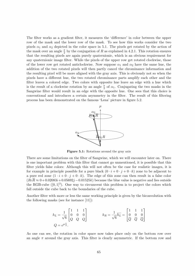
The filter works as a gradient filter, it measures the ‘difference’ in color between the upperrow of the mask and the lower row of the mask. To see how this works consider the twopixels α1 and α2 depicted in the color space in 5.1. The pixels get rotated by the action ofthe mask over an angle π

2 by the conjugation of R as explained in 4.2.1. This rotation ensuresthat the resulting pixels are again purely quaternionic, which is an obvious requirement forany quaternionic image filter. While the pixels of the upper row get rotated clockwise, thoseof the lower row get rotated anticlockwise. Now suppose α1 and α2 have the same hue, theaddition of the two rotated pixels will then partly cancel the chrominance information andthe resulting pixel will be more aligned with the gray axis. This is obviously not so when thepixels have a different hue, the two rotated chrominance parts amplify each other and thefilter leaves a colored edge. Two colors with opposite hue leave an edge with a hue whichis the result of a clockwise rotation by an angle π

2 of α1. Conjugating the two masks in theSangwine filter would result in an edge with the opposite hue. One sees that this choice isconventional and introduces a certain asymmetry in the filter. The result of this filteringprocess has been demonstrated on the famous ‘Lena’ picture in figure 5.2.

µ

α2Rα2R

α1

Rα1R

Figure 5.1: Rotations around the gray axis

There are some limitations on the filter of Sangwine, which we will encounter later on. Thereis one important problem with this filter that cannot go unmentioned, it is possible that thisfilter yields false colors: Although this will not often be the case for realistic images, it isfor example in principle possible for a pure black (0 · i + 0 · j + 0 · k) zone to be adjacent toa pure red zone (1 · i + 0 · j + 0 · k). The edge of this zone can then result in a false color(RcR ≈ 0+0.02083i+0.05692j−0.01525k) because the blue value is negative and lies outsidethe RGB-cube ([0, 1]3). One way to circumvent this problem is to project the colors whichfall outside the cube back to the boundaries of the cube.

Another filter with more or less the same working principle is given by the biconvolution withthe following masks (see for instance [11]):

hL =1√6

1 1 10 0 0Q Q Q

hR =1√6hL =

1 1 10 0 0

Q Q Q

Q = eµ

π2 .

As one can see, the rotation in color space now takes place only on the bottom row overan angle π around the gray axis. This filter is clearly asymmetric. If the bottom row and

65

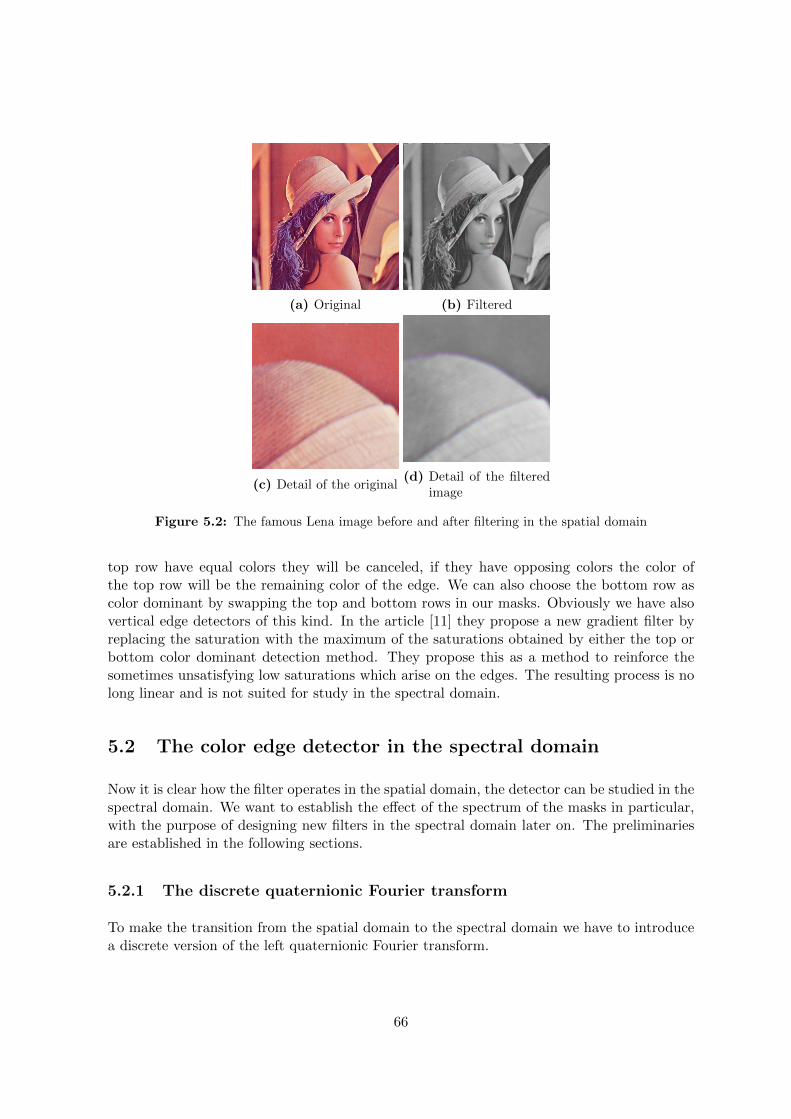
(a) Original (b) Filtered

(c) Detail of the original(d) Detail of the filtered

image

Figure 5.2: The famous Lena image before and after filtering in the spatial domain

top row have equal colors they will be canceled, if they have opposing colors the color ofthe top row will be the remaining color of the edge. We can also choose the bottom row ascolor dominant by swapping the top and bottom rows in our masks. Obviously we have alsovertical edge detectors of this kind. In the article [11] they propose a new gradient filter byreplacing the saturation with the maximum of the saturations obtained by either the top orbottom color dominant detection method. They propose this as a method to reinforce thesometimes unsatisfying low saturations which arise on the edges. The resulting process is nolong linear and is not suited for study in the spectral domain.

5.2 The color edge detector in the spectral domain

Now it is clear how the filter operates in the spatial domain, the detector can be studied in thespectral domain. We want to establish the effect of the spectrum of the masks in particular,with the purpose of designing new filters in the spectral domain later on. The preliminariesare established in the following sections.

5.2.1 The discrete quaternionic Fourier transform

To make the transition from the spatial domain to the spectral domain we have to introducea discrete version of the left quaternionic Fourier transform.

66

Definition 17 The discrete left qFT is defined by:

g(u, v) = Fµ,ν(M,N)[f(m,n)](u, v) =1√MN

M−1∑m=0

N−1∑n=0

e2π(µmuM

+ν nvN

)f(m,n)

The discrete right qFT is defined in a similar way. The inverse discrete left iqFT isgiven by a reversal of the sign of the roots:

f(m,n) = F−µ,−ν(M,N) [g(u, v)](m,n) =1√MN

M−1∑m=0

N−1∑n=0

e−2π(µmuM

+ν nvN

)g(u, v)

Notice that in this definition we have specified the size of the image M by N in the transform;this will be an important point later on. When the transform with just one single root µ isapplied we will denote it as Fµ,µM,N . Because we can choose the roots there will be an infinitenumber of transforms we can apply. As a consequence there is no unique spectrum of theimage and we can only specify the spectrum with respect to a certain transform Fµ,ν(M,N). We

will mostly make use of the transform with one root Fµ,µM,N where µ is the gray axis.

We will now discuss how we have to interpret the spectrum of the qFT, as discovered in thepaper [11]. Let us investigate the effect of a pulse δu0,v0 in the spectrum at a wavevector(u0, v0) on the spatial domain. Such a pulse is defined as

δu0,v0(u, v) =

{q, if (u, v) = (u0, v0)

0, if (u, v) 6= (u0, v0).with q ∈ H

We can easily compute the inverse transform in this case:

√MNF−µ,−µ(M,N) [δu0,v0(u, v)](m,n)

=1√MN

M−1∑m=0

N−1∑n=0

e2π(−µmuM−µnv

N)δu0,v0(u, v)

=q√MN

e2π(−µmu0M−µnv0

N)

=q√MN

(cos (2π(mu0M

+nv0N

))− µ sin (2π(mu0M

+nv0N

))).

It is obvious that this pulse cannot be the spectrum of an image, because the scalar part ofthe inverse transform is nonzero. The fact that the scalar part of an image has to be zeroby definition induces some symmetry in the spectrum g. It is easily proven that the scalarpart of the spectrum S(g)(u, v) needs to be odd and the vectorial part V (g)(u, v) needs to beeven:

67

S(g)(−u,−v) = −S(g)(u, v)

V (g)(−u,−v) = V (g)(u, v)

To obtain a proper image in the inverse transform we have to compensate our pulse with asecond pulse of size −q placed at (−u0,−v0) (or (M − u0, N − v0) which is equivalent due toperiodicity). Indeed, let us calculate the spectrum of δu0,v0 − δ−u0,−v0 :

√MNF−µ,−µ(M,N) [δu0,v0(u, v)− δ−u0,−v0(u, v)](m,n)

= qe2π(−µ(mu0M

+νnv0N

) − qe2π(µ(mu0M

+nv0N

))

= 2[−S(q)µ sin (2π(mu0M

+nv0N

)) + V (q) cos (2π(mu0M

+nv0N

))].

This result is indeed purely quaternionic and represents an image. We conclude that thescalar part of q induces odd luminance oscillations in the direction (u0, v0), while the vectorpart induces oscillations along the color represented by V (q). If for example V (q) = i thiswould induce a spatial variation of the red part of a color. This interpretation is the basis forfiltering by applying qFTs.

5.2.2 Discretization of the convolution formulas

We now want to apply the convolution formulas derived in part I. To do this they need to bediscretized. We will compute the discrete version of (2.15) and derive a set of rules for thediscretization in this process. Notice that the vectors x,y, z and u ∈ N2 are now discrete.(The arguments in u are omitted in the last line for brevity) We obtain the following result:

68

√MNFµ,µM,N [f ∗ h(x1, x2)](u1, u2)

=

M−1∑x1=0

N−1∑x2=0

eµ2π(x1u1M

+x2u2N )f ∗ h(x1, x2)

=M−1∑x1=0

N−1∑x2=0

eµ2π(x1u1M

+x2u2N )

Mm−1∑y1=0

Nm−1∑y2=0

f(x1 − y1, x2 − y2)h(y1, y2)

=

Mm−1∑y1=0

Nm−1∑y2=0

M−1∑x1=0

N−1∑x2=0

eµ2π(x1u1M

+x2u2N

)f(x1 − y1, x2 − y2)h(y1, y2)

=

Mm−1∑y1=0

Nm−1∑y2=0

M−1−y1∑z1=−y1

N−1−y2∑z2=−y2

eµ2π((z1+y1)u1

M+

(z2+y2)u2N

)f(z1, z2)h(y1, y2)

=

Mm−1∑y1=0

Nm−1∑y2=0

M−1∑z1=0

N−1−0∑z2=0

eµ2π((z1+y1)u1

M+

(z2+y2)u2N

)f(z1, z2)h(y1, y2)

=

Mm−1∑y1=0

Nm−1∑y2=0

M−1∑z1=0

N−1−0∑z2=0

eµ2π(z1u1M

+z2u2N

) 1

2[f − µfµ](z1, z2)e

µ2π(y1u1M

+y2u2N

)h(y1, y2)

+

Mm−1∑y1=0

Nm−1∑y2=0

M−1∑z1=0

N−1−0∑z2=0

eµ2π(z1u1M

+z2u2N

) 1

2[f + µfµ](z1, z2)e

−µ2π( y1u1M

+y2u2N

)h(y1, y2)

=MN

2[Fµ,µM,N (f)Fµ,µM,N (g)−Fµ,µM,N (µf)Fµ,µM,N (µg)

+ Fµ,µM,N (f)Fµ,µM,N (g(1,1)) + Fµ,µM,N (µf)Fµ,µM,N (µg(1,1))]

(5.3)

In this derivation we made use of the periodic boundary conditions on f and the periodicityof the exponential to conclude that the sum

∑M−1z1=0

∑N−1−0z2=0 contains the same terms as the

sum∑M−1−y1

z1=−y1∑N−1−y2

z2=−y2 .

Notice that the transform on the mask h has to be computed as if the mask was M by N .. Toachieve this we have to pad h with zeros to this size. There is in fact nothing that prevents usto derive this formula for other values of M and N , but the practical use of such formulas islimited. Suppose that we would choose M and N to be equal to the size of the mask (3× 3),then the convolution formula would still hold but the reconstruction of the image would beimpossible. The qFT with a smaller size on the image leads to an inherent information loss.Let us recall the continuous formula (2.15) in a convenient formulation to make a comparison.

Fµ,µ(f ∗ g(x))

= π[Fµ,µ(f)(u)Fµ,µ(g)−Fµ,µ(µf)Fµ,µ(µg) + Fµ,µ(f)Fµ,µ(g(1,1)) + Fµ,µ(µf)Fµ,µ(µg(1,1))]

On the basis of this calculation we can make a prescription for discretizing other formulasunder the assumption of periodic boundaries conditions. To discretize the formula for acertain image size (M,N) we have to make the following replacements:

69

• Integrals to summations

• Continuous transforms to discrete transforms

• Continuous vectors to discrete ones

• The prefactor

This translates into the following set of rules.

1

2π

∫R2

dx 7→ 1√MN

M−1∑m=0

N−1∑n=0

Fµ,µ 7→ Fµ,µM,N

x ∈ R2 7→ x ∈ {0,M − 1} × {0, N − 1}

2π 7→√MN

70

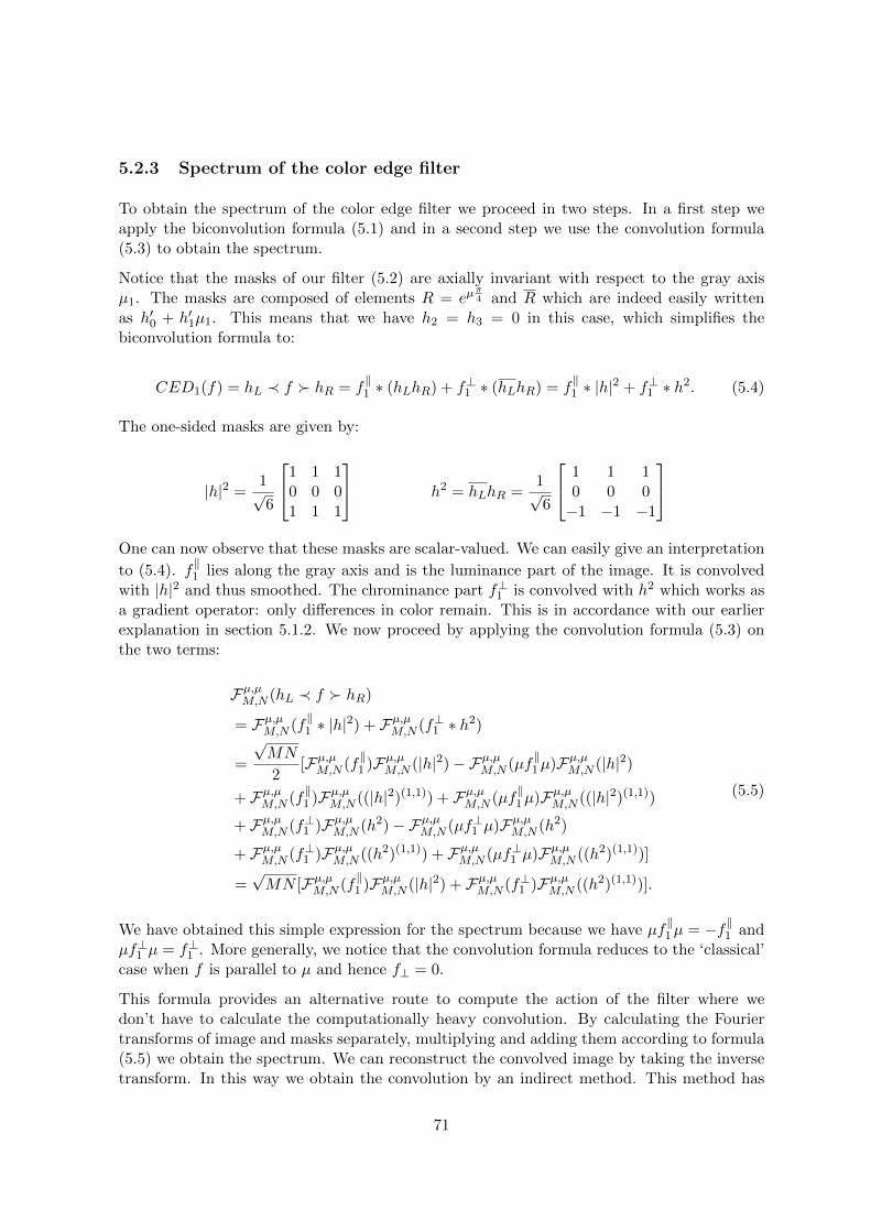
5.2.3 Spectrum of the color edge filter

To obtain the spectrum of the color edge filter we proceed in two steps. In a first step weapply the biconvolution formula (5.1) and in a second step we use the convolution formula(5.3) to obtain the spectrum.

Notice that the masks of our filter (5.2) are axially invariant with respect to the gray axisµ1. The masks are composed of elements R = eµ

π4 and R which are indeed easily written

as h′0 + h′1µ1. This means that we have h2 = h3 = 0 in this case, which simplifies thebiconvolution formula to:

CED1(f) = hL ≺ f � hR = f‖1 ∗ (hLhR) + f⊥1 ∗ (hLhR) = f

‖1 ∗ |h|

2 + f⊥1 ∗ h2. (5.4)

The one-sided masks are given by:

|h|2 =1√6

1 1 10 0 01 1 1

h2 = hLhR =1√6

1 1 10 0 0−1 −1 −1

One can now observe that these masks are scalar-valued. We can easily give an interpretation

to (5.4). f‖1 lies along the gray axis and is the luminance part of the image. It is convolved

with |h|2 and thus smoothed. The chrominance part f⊥1 is convolved with h2 which works asa gradient operator: only differences in color remain. This is in accordance with our earlierexplanation in section 5.1.2. We now proceed by applying the convolution formula (5.3) onthe two terms:

Fµ,µM,N (hL ≺ f � hR)

= Fµ,µM,N (f‖1 ∗ |h|

2) + Fµ,µM,N (f⊥1 ∗ h2)

=

√MN

2[Fµ,µM,N (f

‖1 )Fµ,µM,N (|h|2)−Fµ,µM,N (µf

‖1µ)Fµ,µM,N (|h|2)

+ Fµ,µM,N (f‖1 )Fµ,µM,N ((|h|2)(1,1)) + Fµ,µM,N (µf

‖1µ)Fµ,µM,N ((|h|2)(1,1))

+ Fµ,µM,N (f⊥1 )Fµ,µM,N (h2)−Fµ,µM,N (µf⊥1 µ)Fµ,µM,N (h2)

+ Fµ,µM,N (f⊥1 )Fµ,µM,N ((h2)(1,1)) + Fµ,µM,N (µf⊥1 µ)Fµ,µM,N ((h2)(1,1))]

=√MN [Fµ,µM,N (f

‖1 )Fµ,µM,N (|h|2) + Fµ,µM,N (f⊥1 )Fµ,µM,N ((h2)(1,1))].

(5.5)

We have obtained this simple expression for the spectrum because we have µf‖1µ = −f‖1 and

µf⊥1 µ = f⊥1 . More generally, we notice that the convolution formula reduces to the ‘classical’case when f is parallel to µ and hence f⊥ = 0.

This formula provides an alternative route to compute the action of the filter where wedon’t have to calculate the computationally heavy convolution. By calculating the Fouriertransforms of image and masks separately, multiplying and adding them according to formula(5.5) we obtain the spectrum. We can reconstruct the convolved image by taking the inversetransform. In this way we obtain the convolution by an indirect method. This method has

71

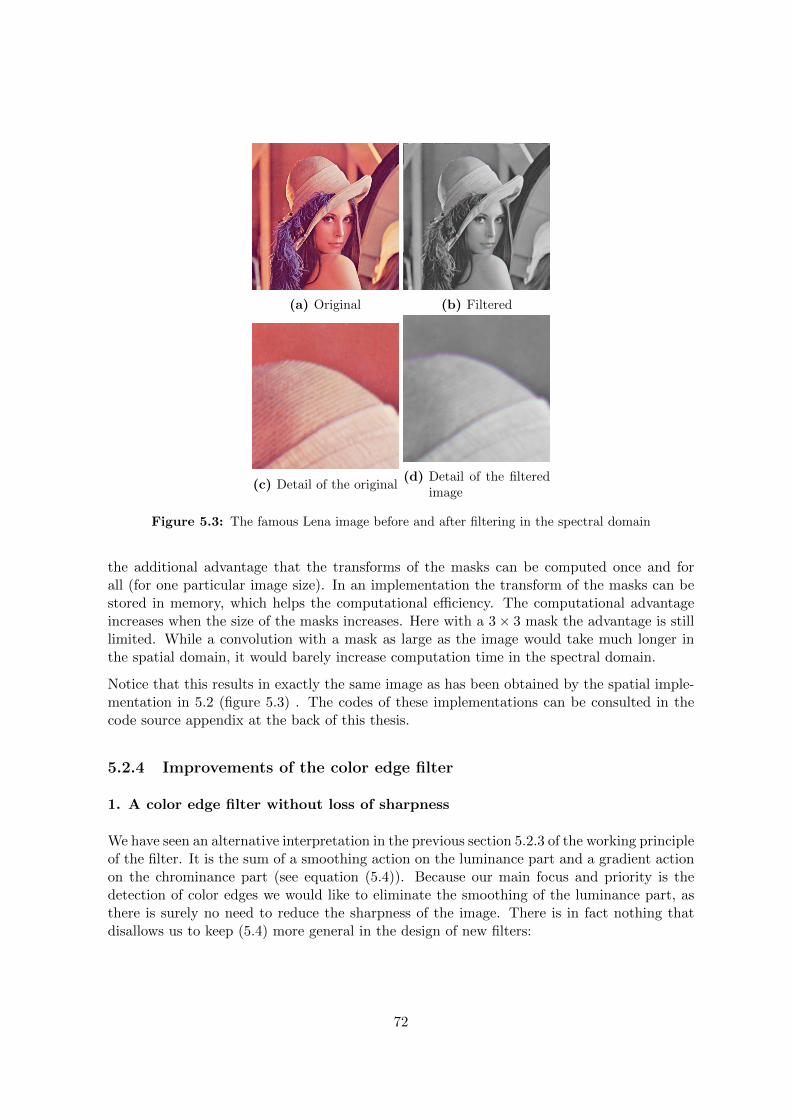
(a) Original (b) Filtered

(c) Detail of the original(d) Detail of the filtered

image

Figure 5.3: The famous Lena image before and after filtering in the spectral domain

the additional advantage that the transforms of the masks can be computed once and forall (for one particular image size). In an implementation the transform of the masks can bestored in memory, which helps the computational efficiency. The computational advantageincreases when the size of the masks increases. Here with a 3× 3 mask the advantage is stilllimited. While a convolution with a mask as large as the image would take much longer inthe spatial domain, it would barely increase computation time in the spectral domain.

Notice that this results in exactly the same image as has been obtained by the spatial imple-mentation in 5.2 (figure 5.3) . The codes of these implementations can be consulted in thecode source appendix at the back of this thesis.

5.2.4 Improvements of the color edge filter

1. A color edge filter without loss of sharpness

We have seen an alternative interpretation in the previous section 5.2.3 of the working principleof the filter. It is the sum of a smoothing action on the luminance part and a gradient actionon the chrominance part (see equation (5.4)). Because our main focus and priority is thedetection of color edges we would like to eliminate the smoothing of the luminance part, asthere is surely no need to reduce the sharpness of the image. There is in fact nothing thatdisallows us to keep (5.4) more general in the design of new filters:

72

CED2(f) = f‖1 ∗A+ f⊥1 ∗B.

This gives us more flexibility than the case A = |h|2 and B = h2, but we have to rememberthat the result of the convolution process needs to be an image. This leads to restrictions onthe elements of A and B. The fact that the result needs to be purely quaternionic translatesinto the requirement CED2(f) = −CED2(f). Because this has to hold for every image f it

has to hold for the luminance part f‖1 and chrominance part f⊥1 separately (we can choose f

to be a gray scale image).

We can derive the following restriction on our choice of A.

f‖1 ∗A(m,n) = −f‖1 ∗A(m,n)

1

3

2∑i=0

2∑j=0

f‖1 (m− i, n− j)A(i, j) = −1

3

2∑i=0

2∑j=0

f‖1 (m− i, n− j)A(i, j)

Choosing our image as such that only one pixel in the neighborhood of (m,n) is not black(nonzero) and making use of the symplectic decompostion of f and A,

f = f ′1µ1 + f ′2µ2 + f ′3µ3 µ1(= µ) ⊥ µ2µ2 ⊥ µ3(= µ1µ2)

f‖1 = f ′1µ1

f⊥1 = f ′2µ2 + f ′3µ3

A = A0 +A1µ1 +A2µ2 +A3µ3

we arrive at:

µ1A(m,n) = −µ1A(m,n) ⇐⇒µ1(A0 +A1µ1 +A2µ2 +A3µ3) = −µ1(A0 +A1µ1 +A2µ2 +A3µ3) ⇐⇒

A0µ1 −A1 +A2µ3 −A3µ2 = −A0µ1 −A1 +A2µ3 −A3µ2 ⇐⇒A0µ1 −A1 +A2µ3 −A3µ2 = A0µ1 +A1 +A2µ3 −A3µ2.

Eventually using the orthogonality {µi, µj} = −2δij we conclude that the only restrictions onthe elements of A are A1 = 0. The µ1 factor in the image selects the vanishing componentA1. A similar reasoning can be made for the B mask but now with the µ2 and µ3 factors off⊥1 . We summarize the results below:

A1 = 0

B2 = B3 = 0.(5.6)

Now we have derived the restrictions on the masks A and B we can try to make a suitablechoice for them. To have the same color effect as the detector of Sangwine without a loss ofsharpness we can choose the following matrices for the masks A and B.

73

A =

0 0 00 1 00 0 0

B = h2 =1√6

1 1 10 0 0−1 −1 −1

(5.7)

We see that this choice indeed satisfies the conditions 5.6. The convolution with A just yieldsthe original luminance part of the image moved over (−1,−1). The image is moved by Ato match the edge detection of the mask B. This results in a color edge filter without theundesired effect of smoothing.

Let us now consider the spectral implementation of this new filter. We can adapt (5.5) tothis more general filter.

Fµ,µM,N (CED2(f)) =√MN [Fµ,µM,N (f

‖1 )Fµ,µM,N (A) + Fµ,µM,N (f⊥1 )Fµ,µM,N ((B)(1,1))]. (5.8)

The mask A works as a Kronecker delta. We know from classical Fourier analysis that a deltagives rise to a constant spectrum in the Fourier domain. We would like to put Fµ,µM,N (A) = 1in (5.8),as this would give us a big computational advantage. The constant spectrum is infact the spectrum of the following mask.

A′ =

1 0 00 0 00 0 0

Convolving with A′ would not move the image to match the edges. But the constant spectrumof A′ is a very good approximation of the spectrum of A in the limit of a large image. Onecan correct for the movement of the image by adapting the spectrum of B instead. Indeed ifwe periodically (with periodic boundary conditions) move the zero padded version of B over(−1,−1) we get a spectrum of B′(x1, x2) = B(x1 + 1, x2 + 1) and only need one mask.

Fµ,µM,N (CED2(f)) =√MN [Fµ,µM,N (f

‖1 ) + Fµ,µM,N (f⊥1 )Fµ,µM,N ((B′)(1,1))]

The resulting images are compared in figure 5.4 below.

74

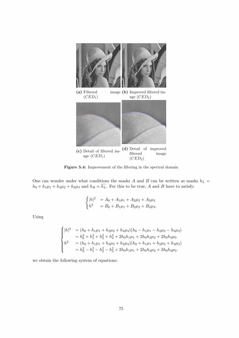
(a) Filtered image(CED1)

(b) Improved filtered im-age (CED2)

(c) Detail of filtered im-age (CED1)

(d) Detail of improvedfiltered image(CED2)

Figure 5.4: Improvement of the filtering in the spectral domain

One can wonder under what conditions the masks A and B can be written as masks hL =h0 + h1µ1 + h2µ2 + h3µ3 and hR = hL. For this to be true, A and B have to satisfy:

{|h|2 = A0 +A1µ1 +A2µ2 +A3µ3

h2 = B0 +B1µ1 +B2µ2 +B3µ3.

Using

|h|2 = (h0 + h1µ1 + h2µ2 + h3µ3)(h0 − h1µ1 − h2µ2 − h3µ3)

= h20 + h21 + h22 + h23 + 2h0h1µ1 + 2h0h2µ2 + 2h0h3µ3

h2 = (h0 + h1µ1 + h2µ2 + h3µ3)(h0 + h1µ1 + h2µ2 + h3µ3)

= h20 − h21 − h22 − h23 + 2h0h1µ1 + 2h0h2µ2 + 2h0h3µ3.

we obtain the following system of equations:

75

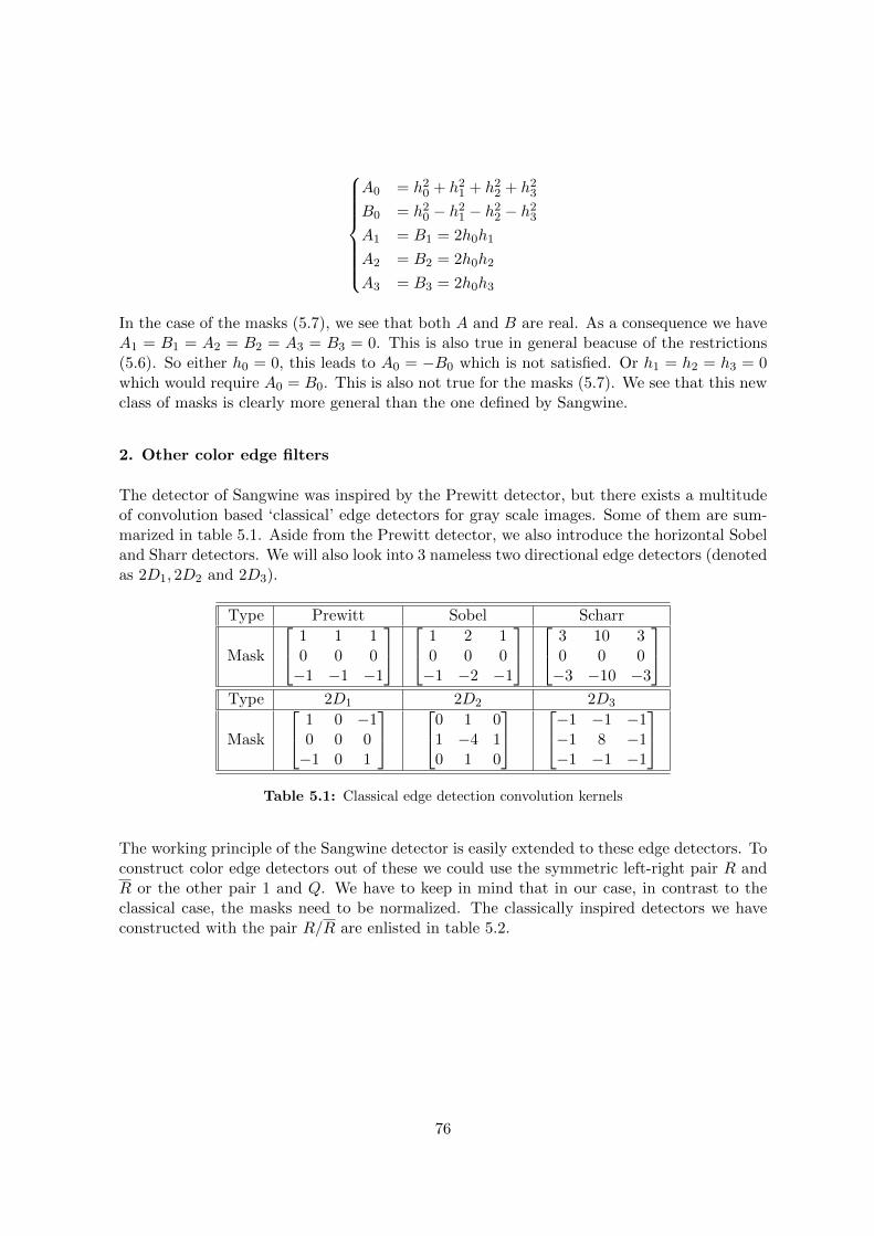
A0 = h20 + h21 + h22 + h23B0 = h20 − h21 − h22 − h23A1 = B1 = 2h0h1

A2 = B2 = 2h0h2

A3 = B3 = 2h0h3

In the case of the masks (5.7), we see that both A and B are real. As a consequence we haveA1 = B1 = A2 = B2 = A3 = B3 = 0. This is also true in general beacuse of the restrictions(5.6). So either h0 = 0, this leads to A0 = −B0 which is not satisfied. Or h1 = h2 = h3 = 0which would require A0 = B0. This is also not true for the masks (5.7). We see that this newclass of masks is clearly more general than the one defined by Sangwine.

2. Other color edge filters

The detector of Sangwine was inspired by the Prewitt detector, but there exists a multitudeof convolution based ‘classical’ edge detectors for gray scale images. Some of them are sum-marized in table 5.1. Aside from the Prewitt detector, we also introduce the horizontal Sobeland Sharr detectors. We will also look into 3 nameless two directional edge detectors (denotedas 2D1, 2D2 and 2D3).

Type Prewitt Sobel Scharr

Mask

1 1 10 0 0−1 −1 −1

1 2 10 0 0−1 −2 −1

3 10 30 0 0−3 −10 −3

Type 2D1 2D2 2D3

Mask

1 0 −10 0 0−1 0 1

0 1 01 −4 10 1 0

−1 −1 −1−1 8 −1−1 −1 −1

Table 5.1: Classical edge detection convolution kernels

The working principle of the Sangwine detector is easily extended to these edge detectors. Toconstruct color edge detectors out of these we could use the symmetric left-right pair R andR or the other pair 1 and Q. We have to keep in mind that in our case, in contrast to theclassical case, the masks need to be normalized. The classically inspired detectors we haveconstructed with the pair R/R are enlisted in table 5.2.

76

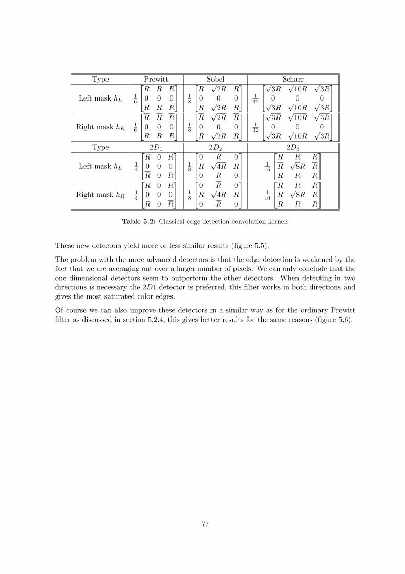
Type Prewitt Sobel Scharr

Left mask hL16

R R R0 0 0

R R R

18

R √2R R

0 0 0

R√

2R R

132

√3R√

10R√

3R0 0 0√3R

√10R

√3R

Right mask hR

16

R R R0 0 0R R R

18

R √2R R

0 0 0

R√

2R R

132

√3R√

10R√

3R0 0 0√3R

√10R

√3R

Type 2D1 2D2 2D3

Left mask hL14

R 0 R0 0 0

R 0 R

18

0 R 0

R√

4R R0 R 0

116

R R R

R√

8R R

R R R

Right mask hR

14

R 0 R0 0 0

R 0 R

18

0 R 0

R√

4R R

0 R 0

116

R R R

R√

8R RR R R

Table 5.2: Classical edge detection convolution kernels

These new detectors yield more or less similar results (figure 5.5).

The problem with the more advanced detectors is that the edge detection is weakened by thefact that we are averaging out over a larger number of pixels. We can only conclude that theone dimensional detectors seem to outperform the other detectors. When detecting in twodirections is necessary the 2D1 detector is preferred, this filter works in both directions andgives the most saturated color edges.

Of course we can also improve these detectors in a similar way as for the ordinary Prewittfilter as discussed in section 5.2.4, this gives better results for the same reasons (figure 5.6).

77

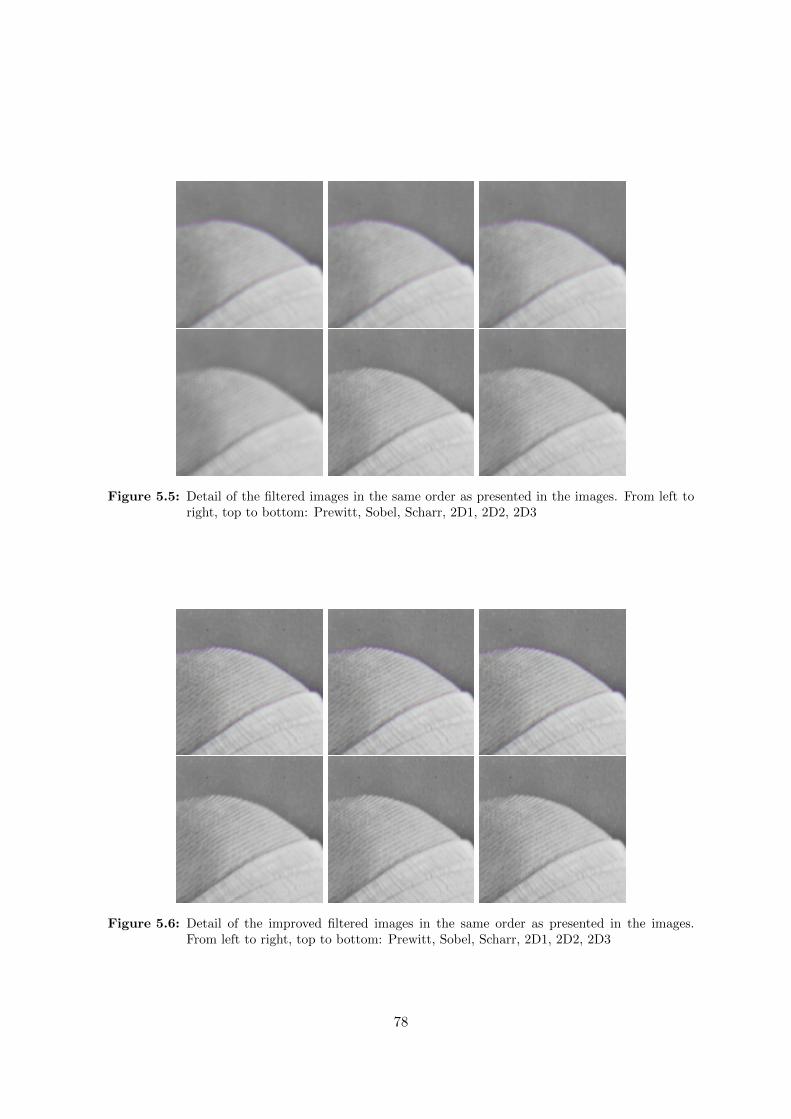
Figure 5.5: Detail of the filtered images in the same order as presented in the images. From left toright, top to bottom: Prewitt, Sobel, Scharr, 2D1, 2D2, 2D3

Figure 5.6: Detail of the improved filtered images in the same order as presented in the images.From left to right, top to bottom: Prewitt, Sobel, Scharr, 2D1, 2D2, 2D3

78

Conclusions

This thesis was divided in two parts. The bulk of the work was situated in the first part.After a short introduction about Clifford algebras we outlined the objective of this thesis, i.e.constructing a formula which expressed the ordinary convolution as a finite linear combinationof Mustard convolutions. This was done in chapter 1. Chapter 2 focused on the special case ofquaternions where the problem is solved in general. In chapter 3 we generalized this approachto general Clifford algebras. There we solved all but the most general case. It is clear thatthese formulas are not unique, but they can easily be rewritten in other forms. The secondpart of the thesis focused on applying the convolution formulas on a ‘toy model’ applicationin image processing. The intuitive geometric interpretations of quaternions lend themselvesto the design of intrinsic color filters. In chapter 4 we introduced the necessary backgroundto study this. In chapter 5 we discussed the spectral implementation of the Sangwine coloredge filter and made some improvements and remarks about these types of filters. To obtainthis spectral implementation the discretized version of the formulas from part I were used.

From a mathematical viewpoint the mere existence of these formulas is perhaps the mostinteresting part of this thesis, the specific form (especially in the general quaternionic case)is more relevant for applications. Although the results are combinatorial in nature they canprovide added value in data analysis. The importance is derived from the intuition behind theClifford numbers as demonstrated by the gray axis µ in our application. The two-dimensionalcase is perhaps too limited to have a structural advantage. Further research is necessary toexplore the domain of multidimensional applications.

79

Bibliography

[1] Spatio-temporal saliency detection using phase spectrum of quaternion fourier transform.Computer Vision and Pattern Recognition, pages 1–8, 2008.

[2] A novel multiresolution spatiotemporal saliency detection model and its applications inimage and video compression. IEEE Trans. Image Process., 19:185–198, 2010.

[3] E. Bayro-Corrochano. Multi-resolution image analysis using the quaternion wavelettransform. Numerical Algorithms, 39:35–55, 2005.

[4] E. Bayro-Corrochano. The theory and use of the quaternion wavelet transform. J. Math.Imaging Vision, 24:19–35, 2006.

[5] F. Brackx, N. De Schepper, and F. Sommen. The Fourier transform in Clifford analysis.Advances in Imaging and Electron Physics, 156:55–201.

[6] F. Brackx, E. Hitzer, and S. Sangwine. History of quaternion and Clifford-fouriertransforms and wavelets, volume 27 of Quaternion and Clifford fourier transforms andwavelets, pages XI–XXVII. Springer Basel AG, 2013.

[7] R. Bujack, H. De Bie, N. De Schepper, and G. Scheuermann. Convolution productsfor hypercomplex fourier transforms. Journal of Mathematical Imaging and Vision,48(3):606–624, 2013.

[8] R. Bujack, G. Scheuermann, and E. Hitzer. A general geometric fourier transform con-volution theorem. Advances in Applied Clifford Algebras, 23(1):15–38, 2013.

[9] H. De Bie. Clifford algebras, Fourier transforms, and quantum mechanics. MathematicalMethods in the Applied Sciences, 35:2198–2228, December 2012.

[10] R. Delanghe. Clifford analysis: History and perspective. Computational Methods andFunction Theory, 1(1):107–153, 2001.

[11] P. Denis, P. Carre, and C. Fernandez-Maloigne. Spatial and spectral quaternionic ap-proaches for colour images. Computer Vision and Image Understanding, 107(1-2):74–87,2007.

[12] L. Dorst, D. Fontijne, and S. Mann. Geometric Algebra for Computer Science: An Object-Oriented Approach to Geometry. Morgan Kaufmann Publishers Inc., San Francisco, CA,USA, 2007.

80

[13] T. A. Ell. Quaternion Fourier Transform: Re-tooling Image and Signal Processing Anal-ysis, volume 27 of Quaternion and Clifford fourier transforms and wavelets, pages XI–XXVII. Springer Basel AG, 2013.

[14] T. A. Ell. Quaternion fourier transform: Re-tooling image and signal processing analysis.pages 3–14, 2013.

[15] T.A. Ell and S.J. Sangwine. Hypercomplex fourier transforms of color images. ImageProcessing, IEEE Transactions on, 16(1):22–35, Jan 2007.

[16] M.D. Fairchild. Color Appearance Models. The Wiley-IS&T Series in Imaging Scienceand Technology. Wiley, 2005.

[17] E. Hitzer. Quaternion fourier transform on quaternion fields and generalizations. Ad-vances in Applied Clifford Algebras, 17(3):497–517, 2007.

[18] S. Kumar, S. Kumar, N. Sukavanam, and B. Raman. Disparity estimation using frac-tional dual tree complex wavelet transform. pages 1–6, Nov 2011.

[19] H.B. Lawson and M.L. Michelsohn. Spin Geometry. Princeton mathematical series.Princeton University Press, 1989.

[20] R. Lukac and K.N. Plataniotis. A taxonomy of color image filtering and enhancementsolutions. Advances in Imaging and Electron Physics, 140:187–264, 2006.

[21] R. Lukac, K.N. Plataniotis, A.N. Venetsanopoulos, R. Bieda, and B. Smolka. Color edgedetection techniques. Signaltheorie und Signalverarbeitung, Akustik und Sprachakustik,Informationstechnik, 29:21–47, 2003.

[22] R. Lukac, B. Smolka, K. Martin, K.N. Plataniotis, and A.N. Venetsanopoulos. Vectorfiltering for color imaging. IEEE Signal Processing Magazine, 22:74–86, 2005.

[23] S-C. Pei, J-J. Ding, and J-H. Chang. Color pattern recognition by quaternion correlation.1:894.

[24] J.M.S Prewitt. Object enhancement and extraction. Picture Processing and Psychopic-torics, 1970.

[25] S.J. Sangwine. Colour image edge detector based on quaternion convolution. ElectronicsLetters, 34(10):969–971, May 1998.

[26] R. Soulard and P. Carre. Quaternionic wavelets for texture classification. Pattern Recog-nition Letters, 32:1669–1678, 2011.

81

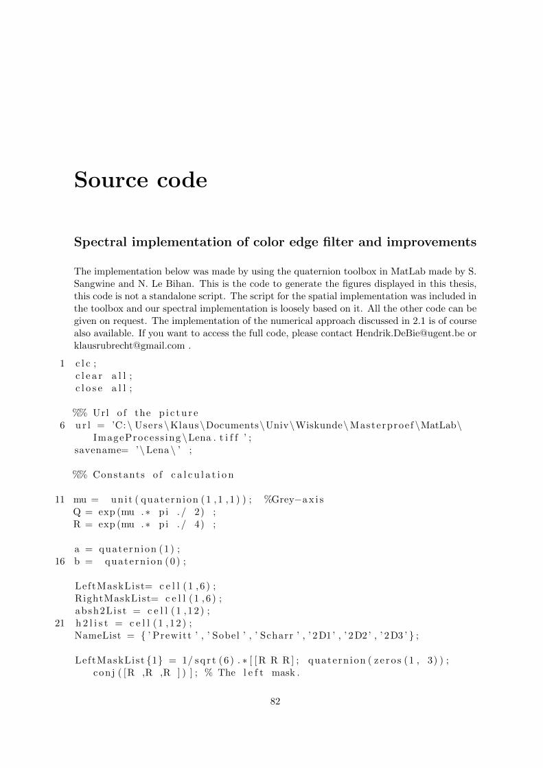
Source code

Spectral implementation of color edge filter and improvements

The implementation below was made by using the quaternion toolbox in MatLab made by S.Sangwine and N. Le Bihan. This is the code to generate the figures displayed in this thesis,this code is not a standalone script. The script for the spatial implementation was included inthe toolbox and our spectral implementation is loosely based on it. All the other code can begiven on request. The implementation of the numerical approach discussed in 2.1 is of coursealso available. If you want to access the full code, please contact Hendrik.DeBie@ugent.be orklausrubrecht@gmail.com .

1 c l c ;c l e a r a l l ;c l o s e a l l ;

%% Url o f the p i c t u r e6 u r l = ’C:\ Users \Klaus\Documents\Univ\Wiskunde\Masterproef \MatLab\

ImageProcess ing \Lena . t i f f ’ ;savename= ’\Lena \ ’ ;

%% Constants o f c a l c u l a t i o n

11 mu = uni t ( quatern ion (1 , 1 , 1 ) ) ; %Grey−a x i sQ = exp (mu .∗ pi . / 2) ;R = exp (mu .∗ pi . / 4) ;

a = quatern ion (1 ) ;16 b = quatern ion (0 ) ;

LeftMaskList= c e l l ( 1 , 6 ) ;RightMaskList= c e l l ( 1 , 6 ) ;absh2Lis t = c e l l ( 1 , 12 ) ;

21 h 2 l i s t = c e l l ( 1 , 12 ) ;NameList = { ’ Prewitt ’ , ’ Sobel ’ , ’ Scharr ’ , ’ 2D1’ , ’ 2D2’ , ’ 2D3 ’ } ;

LeftMaskList {1} = 1/ s q r t (6 ) . ∗ [ [ R R R ] ; quatern ion ( z e r o s (1 , 3) ) ;conj ( [R ,R ,R ] ) ] ; % The l e f t mask .

82

LeftMaskList {2} = 1/ s q r t (8 ) . ∗ [ [ R s q r t (2 ) ∗R R ] ; quatern ion ( z e ro s (1 ,3) ) ; conj ( [R , s q r t (2 ) ∗R ,R ] ) ] ;

26 LeftMaskList {3} = 1/ s q r t (32) .∗ [ [ s q r t (3 ) ∗R s q r t (10) ∗R s q r t (3 ) ∗R ] ;quatern ion ( z e ro s (1 , 3) ) ; conj ( [ s q r t (3 ) ∗R s q r t (10) ∗R s q r t (3 ) ∗R] )] ;

LeftMaskList {4} = 1/ s q r t (4 ) . ∗ [ [ R b conj (R) ] ; quatern ion ( z e r o s (1 , 3)) ; conj ( [R b conj (R) ] ) ] ;

LeftMaskList {5} = 1/ s q r t (8 ) . ∗ [ [ b R b ] ; [ R s q r t (4 ) ∗ conj (R) R ] ; [b ,R ,b ] ] ;

LeftMaskList {6} = 1/ s q r t (16) . ∗ [ [ R R R ] ; [ R s q r t (8 ) ∗ conj (R) R ] ; [R,R ,R ] ] ;

f o r i =1:631 RightMaskList{ i } = conj ( LeftMaskList { i }) ;

absh2Lis t { i } = LeftMaskList { i } .∗ RightMaskList{ i } ;h2L i s t { i } = conj ( LeftMaskList { i }) .∗ RightMaskList{ i } ;absh2Lis t { i +6} =[ quatern ion ( z e ro s (1 , 3) ) ; [ b a b ] ; quatern ion (

z e r o s (1 , 3) ) ] ;h2Li s t { i +6} = h2Lis t { i } ;

36 end

f o r i =1:6ColorEdge ( LeftMaskList { i } , RightMaskList{ i } , ur l , [ savename , NameList{ i} ] )

ColorEdgeSpec ( absh2Lis t { i } , h2L i s t { i } , ur l , [ savename , NameList{ i } ] ) ;41 end

f o r i =7:12ColorEdgeSpec ( absh2Lis t { i } , h2L i s t { i } , ur l , [ savename , NameList{ i −6} , ’

Improved ’ ] ) ;end

46func t i on [ r e s u l t , tElapsed ] = ColorEdge ( l e f t , r i ght , ur l , savename )%COLOREDGE implements the C o l o r E d g e f i l t e r on a p i c t u r e s to r ed in ’

ur l ’% re tu rn s and d i s p l a y s the r e s u l ti f narg in <4

51 savename = ’ Result ’ ;end

mu = uni t ( quatern ion (1 , 1 , 1 ) ) ;d i sp ( [ ’ Reading the image from ’ , u r l ] ) ;

56a = imreadq ( u r l ) ;

qimage = cas t ( imreadq ( u r l ) , ’ double ’ ) . / 255 ;f i g u r e ;

61

83

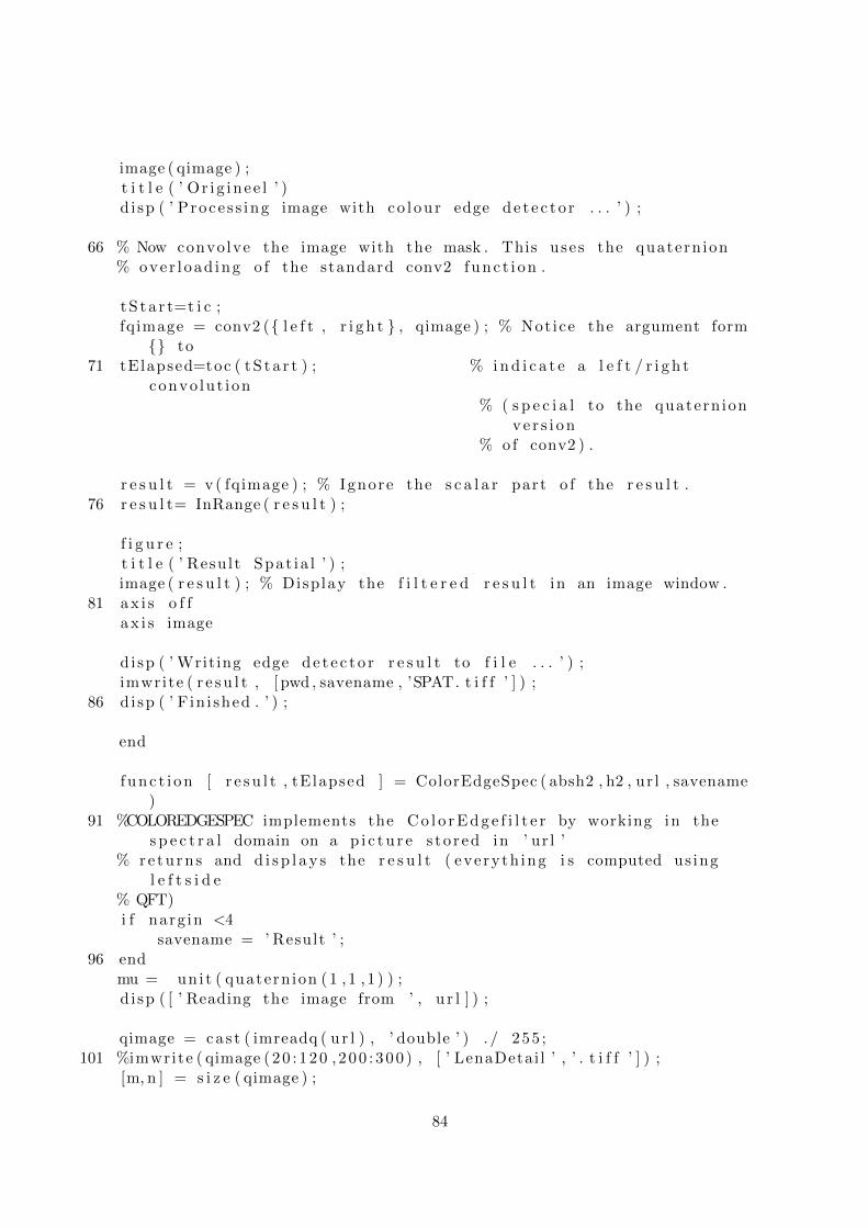
image ( qimage ) ;t i t l e ( ’ Or i g inee l ’ )d i sp ( ’ Proce s s ing image with co l our edge de t e c t o r . . . ’ ) ;

66 % Now convolve the image with the mask . This uses the quatern ion% over l oad ing o f the standard conv2 func t i on .

t S t a r t=t i c ;fqimage = conv2 ({ l e f t , r i g h t } , qimage ) ; % Notice the argument form{} to

71 tElapsed=toc ( t S t a r t ) ; % i n d i c a t e a l e f t / r i g h tconvo lut ion

% ( s p e c i a l to the quatern ionve r s i on

% of conv2 ) .

r e s u l t = v ( fqimage ) ; % Ignore the s c a l a r part o f the r e s u l t .76 r e s u l t= InRange ( r e s u l t ) ;

f i g u r e ;t i t l e ( ’ Result Spat ia l ’ ) ;image ( r e s u l t ) ; % Display the f i l t e r e d r e s u l t in an image window .

81 a x i s o f fa x i s image

d i sp ( ’ Writing edge de t e c t o r r e s u l t to f i l e . . . ’ ) ;imwrite ( r e s u l t , [ pwd , savename , ’SPAT. t i f f ’ ] ) ;

86 d i sp ( ’ F in i shed . ’ ) ;

end

func t i on [ r e s u l t , tElapsed ] = ColorEdgeSpec ( absh2 , h2 , ur l , savename)

91 %COLOREDGESPEC implements the C o l o r E d g e f i l t e r by working in thes p e c t r a l domain on a p i c t u r e s to r ed in ’ ur l ’

% re tu rn s and d i s p l a y s the r e s u l t ( everyth ing i s computed us ingl e f t s i d e

% QFT)i f narg in <4

savename = ’ Result ’ ;96 end

mu = uni t ( quatern ion (1 , 1 , 1 ) ) ;d i sp ( [ ’ Reading the image from ’ , u r l ] ) ;

qimage = cas t ( imreadq ( u r l ) , ’ double ’ ) . / 255 ;101 %imwrite ( qimage (2 0 : 12 0 , 2 00 : 300 ) , [ ’ LenaDetai l ’ , ’ . t i f f ’ ] ) ;

[m, n ] = s i z e ( qimage ) ;

84

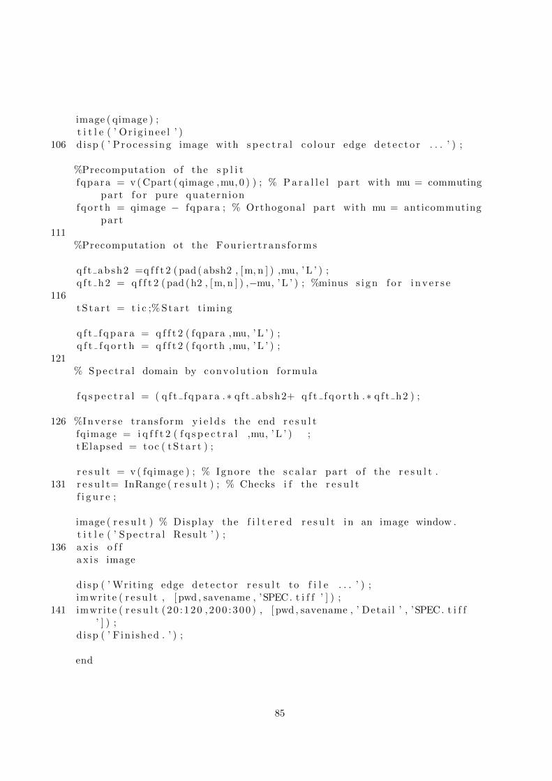
image ( qimage ) ;t i t l e ( ’ Or i g inee l ’ )

106 d i sp ( ’ Proce s s ing image with s p e c t r a l co l our edge de t e c t o r . . . ’ ) ;

%Precomputation o f the s p l i tfqpara = v ( Cpart ( qimage ,mu, 0 ) ) ; % P a r a l l e l part with mu = commuting

part f o r pure quatern ionfqo r th = qimage − fqpara ; % Orthogonal part with mu = anticommuting

part111

%Precomputation ot the Four i e r t rans fo rms

q f t absh2 =q f f t 2 ( pad ( absh2 , [m, n ] ) ,mu, ’ L ’ ) ;q f t h2 = q f f t 2 ( pad ( h2 , [m, n ] ) ,−mu, ’ L ’ ) ; %minus s i gn f o r i n v e r s e

116t S t a r t = t i c ;% Star t t iming

q f t f q p a r a = q f f t 2 ( fqpara ,mu, ’ L ’ ) ;q f t f q o r t h = q f f t 2 ( fqorth ,mu, ’ L ’ ) ;

121% Spec t r a l domain by convo lut ion formula

f q s p e c t r a l = ( q f t f q p a r a .∗ q f t absh2+ q f t f q o r t h .∗ q f t h2 ) ;

126 %Inve r s e trans form y i e l d s the end r e s u l tfqimage = i q f f t 2 ( f q s p e c t r a l ,mu, ’ L ’ ) ;tElapsed = toc ( t S t a r t ) ;

r e s u l t = v ( fqimage ) ; % Ignore the s c a l a r part o f the r e s u l t .131 r e s u l t= InRange ( r e s u l t ) ; % Checks i f the r e s u l t

f i g u r e ;

image ( r e s u l t ) % Display the f i l t e r e d r e s u l t in an image window .t i t l e ( ’ Spe c t r a l Result ’ ) ;

136 a x i s o f fa x i s image

d i sp ( ’ Writing edge de t e c t o r r e s u l t to f i l e . . . ’ ) ;imwrite ( r e s u l t , [ pwd , savename , ’SPEC. t i f f ’ ] ) ;

141 imwrite ( r e s u l t ( 20 : 120 , 20 0 : 3 00 ) , [ pwd , savename , ’ Deta i l ’ , ’SPEC. t i f f’ ] ) ;

d i sp ( ’ F in i shed . ’ ) ;

end

85