Informatization in Production Planning and Control
194
Informatization in Production Planning and Control A Simulation based Evaluation of the Impacts in Flow-Shop Production Systems Dipl.-Ing. Christoph Wolfsgruber Doctoral Thesis to achieve the university degree of Doktor der technischen Wissenschaften submitted to Graz University of Technology First Referee Univ.-Prof. Dipl.-Ing. Dr.techn. Siegfried Vössner Second Referee Univ.-Prof. Mag.et Dr.rer.soc.oec. Helmut Zsifkovits Graz, January 2016
Transcript of Informatization in Production Planning and Control
Informatization in
Production Planning and Control A Simulation based Evaluation of the Impacts
in Flow-Shop Production Systems
Dipl.-Ing. Christoph Wolfsgruber
Doctoral Thesis to achieve the university degree of
Doktor der technischen Wissenschaften
submitted to
Graz University of Technology
First Referee
Univ.-Prof. Dipl.-Ing. Dr.techn. Siegfried Vössner
Second Referee
Univ.-Prof. Mag.et Dr.rer.soc.oec. Helmut Zsifkovits
Graz, January 2016

I
Affidavit
I declare that I have authored this thesis independently, that I have not used
other than the declared sources/resources, and that I have explicitly indicated all
material which has been quoted either literally or by content from the sources
used. The text document uploaded to TUGRAZonline is identical to the present
doctoral thesis.
…………………………… …………………………………………………..
Date Signature

II
Acknowledgement
I would like to express my gratitude to my supervisor Prof. Siegfried Vössner for
his comments and remarks. Furthermore, I would like to thank my colleagues
Gerald, Dietmar, Nik and Julia for the inspiring discussions. In addition, I would
like to thank Herbert Steiner for his trust and the chances to apply my knowledge
in several industrial projects. Also, I would like to thank my parents Ludwig and
Siglinde who supported me throughout the entire study and during the process
of thesis writing. My special thanks are extended to Nina for supporting me with
all possible means through the scientific journey.
Christoph Wolfsgruber
III
Abstract
The manufacturing industry of today is coined by the increasing dynamics of the
markets. Products are demanded in increasing varieties, the product life cycles
are getting shorter and demands fluctuate more and more. These trends are
pushing the complexity in production planning and control to new levels.
However, the future also offers new promising opportunity. The informatization
in manufacturing has reached after 40 years of the first computer integrated
manufacturing concepts the shop floor. Internet of things and cyber physical
systems are seen as the enabling technologies behind the visionary concept of
Industry 4.0. These technologies will change the production planning and control
in many ways. Data quality will increase dramatically, status updates from the
shop floor and the tracking of all activities and objects will be available in real
time.
These developments lead to the request of the evaluation of different production
planning and control methods regarding the challenges and opportunities of these
developments. This thesis presents a simulation based evaluation study which
analyzes the impacts of informatization in production planning and control in
flow-shop production systems of automotive industry. Especially the relationships
between data quality and planning model accuracy with respect to the requested
product flexibility is analyzed in this doctoral thesis. Based on the found insights,
a best practice approach for the optimal configuration of a production planning
and control system is deduced.
IV
Table of Content
Introduction ................................................................................... 1
1.1 Industrial Trends .................................................................................... 2
1.1.1 Increasing competitive pressure and globalization ........................ 2
1.1.2 Individualization of products ........................................................ 3
1.1.3 Informatization of production ....................................................... 4
1.2 Motivation .............................................................................................. 5
1.3 Research Question .................................................................................. 7
1.4 Research Methodology ............................................................................ 9
Production and Operations M anagement ..................................... 12
2.1 Definitions ............................................................................................ 13
2.1.1 Production and Operations Management ................................... 13
2.1.2 Logistics ..................................................................................... 14
2.2 Milestones and Hypes ........................................................................... 16
2.2.1 Historical Milestones .................................................................. 16
2.2.2 Recent Developments ................................................................. 21
2.2.3 Ongoing Trends and Hypes ........................................................ 22
2.3 Objectives and Relationships ................................................................ 25
2.3.1 Strategic and Operational Objectives ......................................... 25
2.3.2 Fundamental Relationship between Objectives .......................... 26
2.3.3 Influence of Variability ............................................................... 27
2.4 Variability ............................................................................................ 30
V
2.4.1 Definitions .................................................................................. 30
2.4.2 Internal Variability..................................................................... 32
2.4.3 External Variability ................................................................... 34
2.5 Flexibility and associated Properties .................................................... 35
2.5.1 Flexibility ................................................................................... 35
2.5.2 Agility and Adaptability ............................................................ 37
Informatization in Production ...................................................... 39
3.1 Definitions ............................................................................................ 40
3.1.1 Data, Information, Knowledge, Understanding, Wisdom ........... 40
3.1.2 Informatization ........................................................................... 42
3.2 IT in Production ................................................................................... 43
3.2.1 Computer Integrated Manufacturing .......................................... 43
3.2.2 Digital Factory ........................................................................... 46
3.2.3 Internet of Things ...................................................................... 47
3.2.4 Cyber Physical Systems .............................................................. 48
3.2.5 Industry 4.0 ................................................................................ 50
3.3 IT in Production Planning and Control ................................................ 52
3.3.1 Complexity and Decentralized Decision Making ........................ 52
3.3.2 Data Quality .............................................................................. 55
Production Planning and Control ................................................ 58
4.1 Definitions ............................................................................................ 59
4.1.1 Production Planning ................................................................... 59
4.1.2 Production Control ..................................................................... 60
4.2 Decomposition, Aggregation and Disaggregation .................................. 62
4.3 Production Planning and Control Process ............................................ 65
4.3.1 Planning approaches ................................................................... 65
4.3.2 Hierarchical Process ................................................................... 66
VI
4.3.3 Forecasting ................................................................................. 67
4.3.4 Aggregate Planning .................................................................... 69
4.3.5 Master Production Scheduling .................................................... 70
4.4 Evolution of PPC Systems .................................................................... 72
4.4.1 Reorder Point Systems and Economic Order Quantity .............. 72
4.4.2 Material Requirements Planning ................................................ 75
4.4.3 Extensions to Material Requirements Planning .......................... 80
4.4.4 Just-in-Time and Lean ............................................................... 82
4.4.5 Optimized Production Technology ............................................. 90
4.5 Push and Pull Principles ...................................................................... 91
4.5.1 Definitions .................................................................................. 91
4.5.2 Comparison Studies .................................................................... 92
Simulation based Evaluation Study ............................................. 97
5.1 Modelling Approach.............................................................................. 98
5.1.1 Modelling Techniques ................................................................. 99
5.1.2 Aim and Focus ......................................................................... 101
5.1.3 Simplifications and Assumptions .............................................. 104
5.2 Model Design ...................................................................................... 106
5.2.1 General Structure ..................................................................... 106
5.2.2 Customer Model ....................................................................... 107
5.2.3 Manufacturing Model ............................................................... 109
5.2.4 PPC-Methods ........................................................................... 112
5.3 Evaluation of Informatization and Demand Flexibility ...................... 121
5.3.1 Settings..................................................................................... 121
5.3.2 Results ...................................................................................... 125
5.4 Evaluation of the Supply Variability .................................................. 132
5.4.1 Settings..................................................................................... 132
VII
5.4.2 Results ...................................................................................... 137
Discussion .................................................................................... 141
6.1 Insights ............................................................................................... 142
6.2 Best Practice ...................................................................................... 145
6.2.1 PPC Selection Approach .......................................................... 145
6.2.2 Use Case Example .................................................................... 148
6.3 Lessons Learned .................................................................................. 151
Conclusion ................................................................................... 152
7.1 Research Question .............................................................................. 153
7.2 Further Research ................................................................................ 153
List of Figures .................................................................................. 154
List of Tables ................................................................................... 158
List of Abbreviation ......................................................................... 159
Bibliography .................................................................................... 162
Appendix ......................................................................................... 174
Introduction
It is not the strongest of the species that
survives, nor the most intelligent, but
rather the one most adaptable to change. Charles Darwin (1809 – 1882)
Already 500 years before Christ Heraclitus1 claimed “nothing endures but change”
and the change itself seems to have gathered more momentum in the recent years.
Industrial production companies are operating nowadays in an extremely
turbulent environment (Westkämper & Zahn, 2009; Nyhuis, et al., 2008). This
environment is characterized by the rapid spread of new technologies, new often
very offensive competitors, and ever tighter supply chain network. Products are
demanded in increasing model varieties, the product life cycles are getting shorter
and demands fluctuate more and more. In order to maintain the competitiveness,
companies must be able to respond to these turbulences quickly and flexible
(Nyhuis, et al., 2008). As the main focus of this thesis is in the automotive
industry, an overview of ongoing mega trends in that industry sector is given.
Next, the motivation as well as the gaps for this thesis are described. In the last
section of this chapter the research question, the focus and the used research
methodology is defined.
1 Heraclitus of Ephesus (535 BC – 475 BC) was a Greek philosopher who is famous for his insistence on
ever-present change in the universe
C H A P T E R
INTRODUCTION 2
1.1 Industrial Trends
The developments in manufacturing especially in automotive industry show three
major ongoing trends over the past years, which will have significant impact on
the future global production structures (Krog & Statkevich, 2008; KPMG, 2010;
McKinsey & Company, 2013; Plattform Industrie 4.0, 2013; International Data
Corporation, 2014):
Trend 1: Increasing competitive pressure and globalization
Trend 2: Individualization of products
Trend 3: Informatization of production
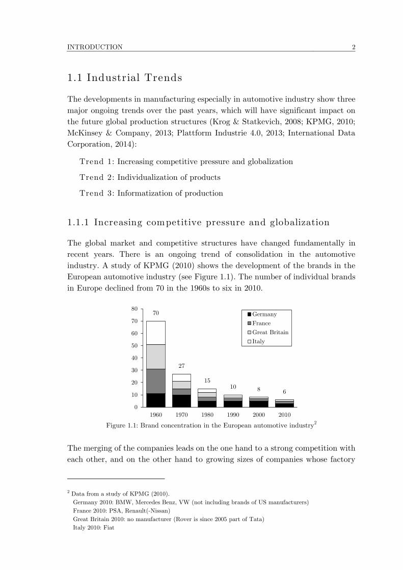
1.1.1 Increasing competitive pressure and globalization
The global market and competitive structures have changed fundamentally in
recent years. There is an ongoing trend of consolidation in the automotive
industry. A study of KPMG (2010) shows the development of the brands in the
European automotive industry (see Figure 1.1). The number of individual brands
in Europe declined from 70 in the 1960s to six in 2010.
Figure 1.1: Brand concentration in the European automotive industry
2
The merging of the companies leads on the one hand to a strong competition with
each other, and on the other hand to growing sizes of companies whose factory
2 Data from a study of KPMG (2010).
Germany 2010: BMW, Mercedes Benz, VW (not including brands of US manufacturers)
France 2010: PSA, Renault(-Nissan)
Great Britain 2010: no manufacturer (Rover is since 2005 part of Tata)
Italy 2010: Fiat
70
27
1510 8 6
0
10
20
30
40
50
60
70
80
1960 1970 1980 1990 2000 2010
Germany
France
Great Britain
Italy
INTRODUCTION 3
networks are stronger and more complexly linked together (KPMG, 2010). The
overall strategic objectives, the production at highest possible yield with given
resources (resource productivity) and the lowest use of resources for a given
production volume (resource efficiency) will also stay the same in future
(Plattform Industrie 4.0, 2013). To master the complexity of highly
interconnected production networks that operate at peak productivity, the need
for development in the area of production planning and control is obvious.
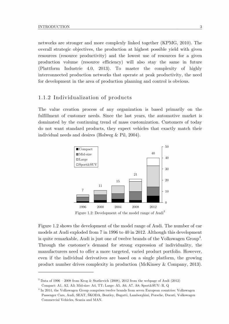
1.1.2 Individualization of products
The value creation process of any organization is based primarily on the
fulfillment of customer needs. Since the last years, the automotive market is
dominated by the continuing trend of mass customization. Customers of today
do not want standard products, they expect vehicles that exactly match their
individual needs and desires (Holweg & Pil, 2004).
Figure 1.2: Development of the model range of Audi
3
Figure 1.2 shows the development of the model range of Audi. The number of car
models at Audi exploded from 7 in 1996 to 40 in 2012. Although this development
is quite remarkable, Audi is just one of twelve brands of the Volkswagen Group4.
Through the customer’s demand for strong expression of individuality, the
manufacturers need to offer a more targeted, varied product portfolio. However,
even if the individual derivatives are based on a single platform, the growing
product number drives complexity in production (McKinsey & Company, 2013).
3 Data of 1996 – 2008 from Krog & Statkevich (2008), 2012 from the webpage of Audi (2012)
Compact: A1, A2, A3; Mid-size: A4, TT; Large: A5, A6, A7, A8; Sport&SUV: R, Q 4 In 2014, the Volkswagen Group comprises twelve brands from seven European countries: Volkswagen
Passenger Cars, Audi, SEAT, ŠKODA, Bentley, Bugatti, Lamborghini, Porsche, Ducati, Volkswagen
Commercial Vehicles, Scania and MAN.
7
11
15
21
40
0
10
20
30
40
50
1996 2000 2004 2008 2012
Compact
Mid-size
Large
Sport&SUV
INTRODUCTION 4
An additional aspect in the individualization of products are the changing regional
and segment patterns to which the car manufacturers have to adapt their
production supply chains, and portfolios. McKinsey & Company (2013) claim
“…the potential for portfolio mis-match as smaller vehicle classes are growing
more strongly than others in fast-growing emerging markets.”
In order to maintain the competitiveness, companies must offer an increasing
number of varieties, which also leads to a higher fluctuation of demands and
diverse product mixes. Operating in such a turbulent environment demands from
companies of today to be able to quickly and flexible respond to these turbulences.
1.1.3 Informatization of production
The rise of internet connections, storage capacities and computation power in an
exponential way over the last years is not expected to decline. The International
Data Corporation (IDC) estimated the digital universe5 in the year 2013 by 4.4
zettabyte6 and is expecting a rise to 44 zettabyte in the year 2020 (International
Data Corporation, 2014). The connection of physical things via the internet called
Internet of Things (IoT) will contribute an increasingly large share to the digital
universe. According to the IDC (2014) 2% of the world wide digital universe was
generated by IoT embedded systems in 2013 and they expect that this share will
rise beyond 10% in 2020. The real time availability of information will lead to
more efficient and intelligent operations. One concept which is driving the
informatization of production is the future project of the German high-tech
strategy called Industry 4.0, which promotes the computerization of
manufacturing. IoT, mobile internet, automation of knowledge work and
advanced robotics is seen as the potentially disruptive technologies related to
Industry 4.0 (McKinsey & Company, 2014). Also the horizontal and vertical
system integration, simulation and large scale data analytics are seen as the
technologies that will transform industrial production (Boston Consulting Group,
2015). Overall, these technologies will also have major impacts on the ways
production is planned and controlled.
5 The digital universe is a measure of all the digital data created, replicated, and consumed in a single
year. 6 1 zettabyte equals 1021 byte
INTRODUCTION 5
1.2 M otivation
The above described trends have a considerable influence on the supply chain
management (SCM) of today’s companies. Driven by the increasing competitive
pressure, it is a must for companies to operate their supply chain optimally.
However, the huge complexity of modern globalized manufacturing networks, or
even single production sides with a high number of individualized products is
forcing companies to make compromises. Nowadays most manufacturer optimize
locally using simple planning models with data which are often of poor quality.
Ten years ago Deloitte (2003) claimed this optimization paradox as one of the
critical trends driven by complexity.
Despite the potentially huge economies from designing supply
chains from a global view, most manufacturers optimize locally.
Manufacturers are spreading supply chain operations across the
world. Yet, most still appear to be optimizing their supply chains
on a “local” basis – by product, function (say, production),
facility, country, or region. This means they are losing
opportunities for large-scale efficiencies. (Deloitte, 2003)
Nowadays, the situation looks the same. The major reason for this optimization
paradox are the missing mathematical tools for production planning. Already 50
years ago Conway et al. (1967) stated the frustrating complexity of the so called
job shop problem, which describes the assignment of jobs to resources at
particular times.
The general job shop problem is a fascinating challenge. Although
it is easy to state, and to visualize what is required, it is extremely
difficult to make any progress whatever toward a solution. Many
proficient people have considered the problem, and all have come
away essentially empty-handed. Since this frustration is not
reported in literature, the problem continues to attract
investigators, who just cannot believe that a problem so simply
structured can be so difficult until they have tried it. (Conway,
et al., 1967)
Now, 50 years later, branch-and-bound algorithms, constraint programming and
heuristic optimization methods can solve slightly bigger problems but there was
no fundamental breakthrough. Only for the individual areas of production
planning, concepts and methods exist such as lot sizing, master planning, etc. but
there is no comprehensive, holistic solution. Furthermore, the models these
methods are using are based on simplifications of some sort, because the real
INTRODUCTION 6
world is too complex to analyze directly (Hopp & Spearman, 2008). However, the
new possibilities of computation offer some promising results. Agent based
computation and real time availability of data will play a major role in the next
generation of production planning and control methods. Also in Industry 4.0, the
following research recommendations are stated to tackle the optimization paradox
of production planning (Plattform Industrie 4.0, 2013):
Development of methods and concepts to increase resource efficiency by
viewing the overall optimum.
Development of new strategies and algorithms which fulfill the need for
higher flexibility. This includes optimized planning and control strategies
for adaptable production systems.
The vision of Industry 4.0 is an intelligent planning and control system based on
a continuous real-time simulation that automatically is rescheduling the
production based on the requirements and the available resources. This vision is
also shared by Schenk et al. (2013) and Nyhuis et al. (2008).
In addition to that vision, many other literature sources describe gaps in the
theory of production planning. Krishnamurthy et al. (2004) stated the lack of
quantitative studies that analyzes the performance of material control strategies
in manufacturing environments with multiple products and diverse product
mixes. Jodlbauer & Huber (2008) recommend research in the robustness and
stability of production planning and control strategies in complex job-shop
environments or real-world applications.
An even almost open field in theory is the added value of high quality data in
production planning. Recently, the impact of inventory inaccuracy in SCM were
analyzed (Fleisch & Tellkamp, 2005) but there is still only limited amount of
research on the effects of informatization on PPC available.
This all leads to the motivation of research in the field of production planning
under the perspective of the need of more flexible production systems due to the
increasing complexity driven. Thereby also the promising new possibilities due to
informatization and their impacts on the performance of the production system
are of interest.
INTRODUCTION 7
1.3 Research Question
Based on the above described industry trends, as well as the gaps in literature,
this thesis deals with the question of which production planning and control
method allow the efficient production of mass customized products under the use
of new opportunities through the ongoing informatization in manufacturing.
Due to different industry and production process properties it is necessary to focus
on a clearly defined domain for answering this question in-detail. Driven through
the experience of several industrial projects the selected focus domain is the
supply industry of automotive production.
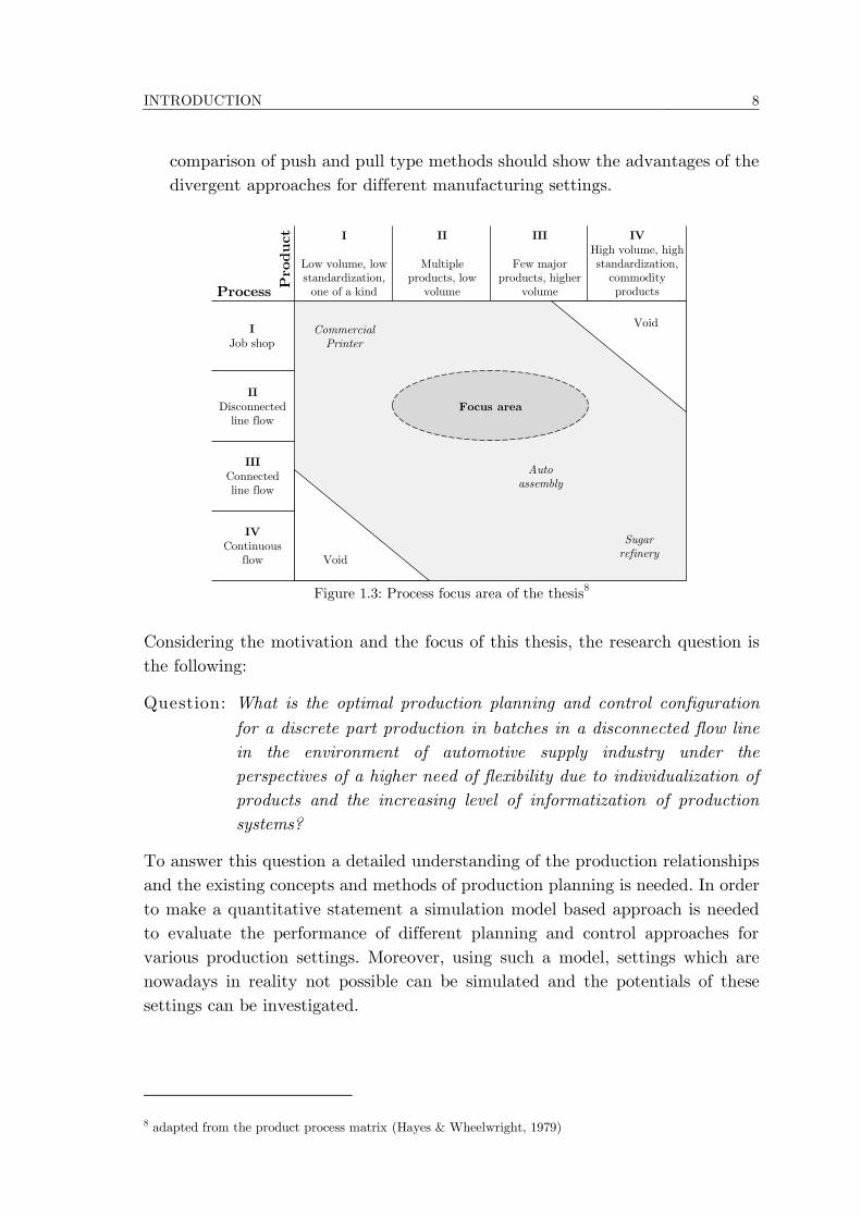
To specify this focus in more detail, the process product matrix of Hayes &
Wheelwright (1979) is used, which classifies manufacturing environments by their
process structure into four categories (Hopp & Spearman, 2008):
Job shop: Small lots are produced with high variety of routings through
the plant. The flow through the plant is jumbled and setups are common.
Disconnected flow lines: Product batches are produced on a limited
number of identifiable paths through the plant. The individual stations
within a path are not connected by a material handling system, so that
inventory can build up between stations.
Connected line flow: The product is fabricated and assembled along a
rigid routing connected by a material handling system. This is the classical
moving assembly line made famous by Henry Ford7.
Continuous flow process: The product (food, chemicals, etc.) flows
automatically down a fixed routing.
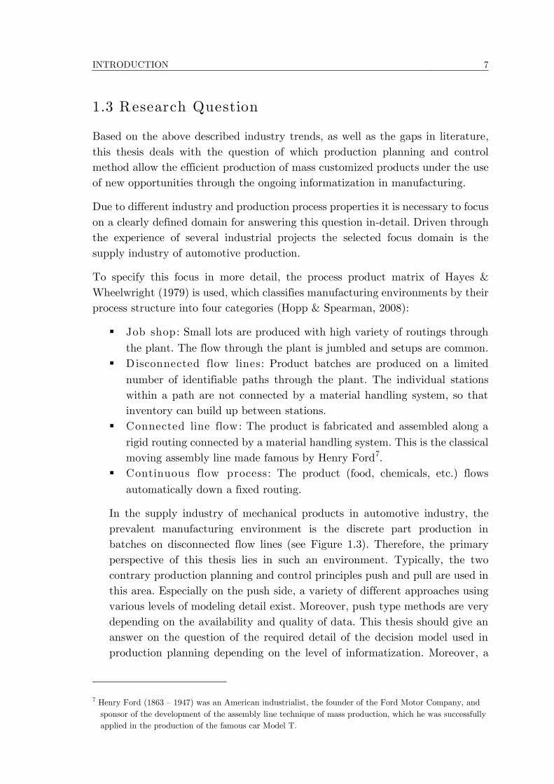
In the supply industry of mechanical products in automotive industry, the
prevalent manufacturing environment is the discrete part production in
batches on disconnected flow lines (see Figure 1.3). Therefore, the primary
perspective of this thesis lies in such an environment. Typically, the two
contrary production planning and control principles push and pull are used in
this area. Especially on the push side, a variety of different approaches using
various levels of modeling detail exist. Moreover, push type methods are very
depending on the availability and quality of data. This thesis should give an
answer on the question of the required detail of the decision model used in
production planning depending on the level of informatization. Moreover, a
7 Henry Ford (1863 – 1947) was an American industrialist, the founder of the Ford Motor Company, and
sponsor of the development of the assembly line technique of mass production, which he was successfully
applied in the production of the famous car Model T.
INTRODUCTION 8
comparison of push and pull type methods should show the advantages of the
divergent approaches for different manufacturing settings.
Figure 1.3: Process focus area of the thesis
8
Considering the motivation and the focus of this thesis, the research question is
the following:
Question: What is the optimal production planning and control configuration
for a discrete part production in batches in a disconnected flow line
in the environment of automotive supply industry under the
perspectives of a higher need of flexibility due to individualization of
products and the increasing level of informatization of production
systems?
To answer this question a detailed understanding of the production relationships
and the existing concepts and methods of production planning is needed. In order
to make a quantitative statement a simulation model based approach is needed
to evaluate the performance of different planning and control approaches for
various production settings. Moreover, using such a model, settings which are
nowadays in reality not possible can be simulated and the potentials of these
settings can be investigated.
8 adapted from the product process matrix (Hayes & Wheelwright, 1979)
I
Low volume, low standardization,
one of a kind
II
Multiple products, low
volume
III
Few major products, higher
volume
IVHigh volume, high standardization,
commodity products
Pro
duct
IJob shop
IIDisconnected
line flow
IIIConnected line flow
IVContinuous
flow
Process
Focus area
Commercial Printer
Autoassembly
Sugar refinery
Void
Void
INTRODUCTION 9
1.4 Research M ethodology
In this thesis a simulation approach is used to develop a theory that gives an
answer on the above stated research question. Especially in the area of production
and operational management (POM) and operational research (OR) simulation
is a key technique for science. Davis et al. (2007) describe the increasingly
significant methodological approach of simulation for the development of theory.
Simulation can provide superior insight into complex theoretical
relationships among constructs, especially when challenging
empirical data limitations exist. (Davis, et al., 2007)
Davis et al. (2007) suggest the following roadmap which is also used in this thesis:
1. Determine a theoretically intriguing research question
2. Identify simple theory that addresses the research question
3. Choose simulation approach that fits with research question,
assumptions, and theoretical logic
4. Create computational representation
5. Verify computational representation
6. Experiment to build novel theory
7. Validate with empirical data
Thereby the research process begins with the formulation of a research question
(1) on a theoretically relevant issue. In the next step (2) the relevant simple
theory is identified and theoretical logic, propositions, constructs, and
assumptions are used to form the basis of the computational representation. By
simple theory, Davis et al. (2007) mean “undeveloped theory … which includes
basic processes that may be known but that have interactions that are only
vaguely understood, if at all”. Before the creation of the simulation model, the
roadmap suggests to select an appropriate simulation approach (3) that fits with
the research question, assumptions, and theoretical logic. The central activity in
the research process is the creation of the computational representation (4).
According to Davis et al. (2007) this activity involves “(a) operationalizing the
theoretical constructs, (b) building the algorithms that mirror the theoretical logic
of the focal theory, and (c) specifying assumptions that bound the theory and
results”. The verification of the computational representation (5) confirms the
accuracy and the robustness of the computational representation as well as the
internal validity of the theory. The experiment step (6) is the heart of the
roadmap for developing the novel theory. There are several approaches for
effective experimentation: (a) varying value that were held constant in the initial
simple theory, (b) breaking a single construct into constituent component
INTRODUCTION 10
constructs, (c) varying assumptions and (d) adding new features to the
computational representation. The final step in theory development using
simulation methods is validation (7), which involves the comparison of simulation
results with empirical data.
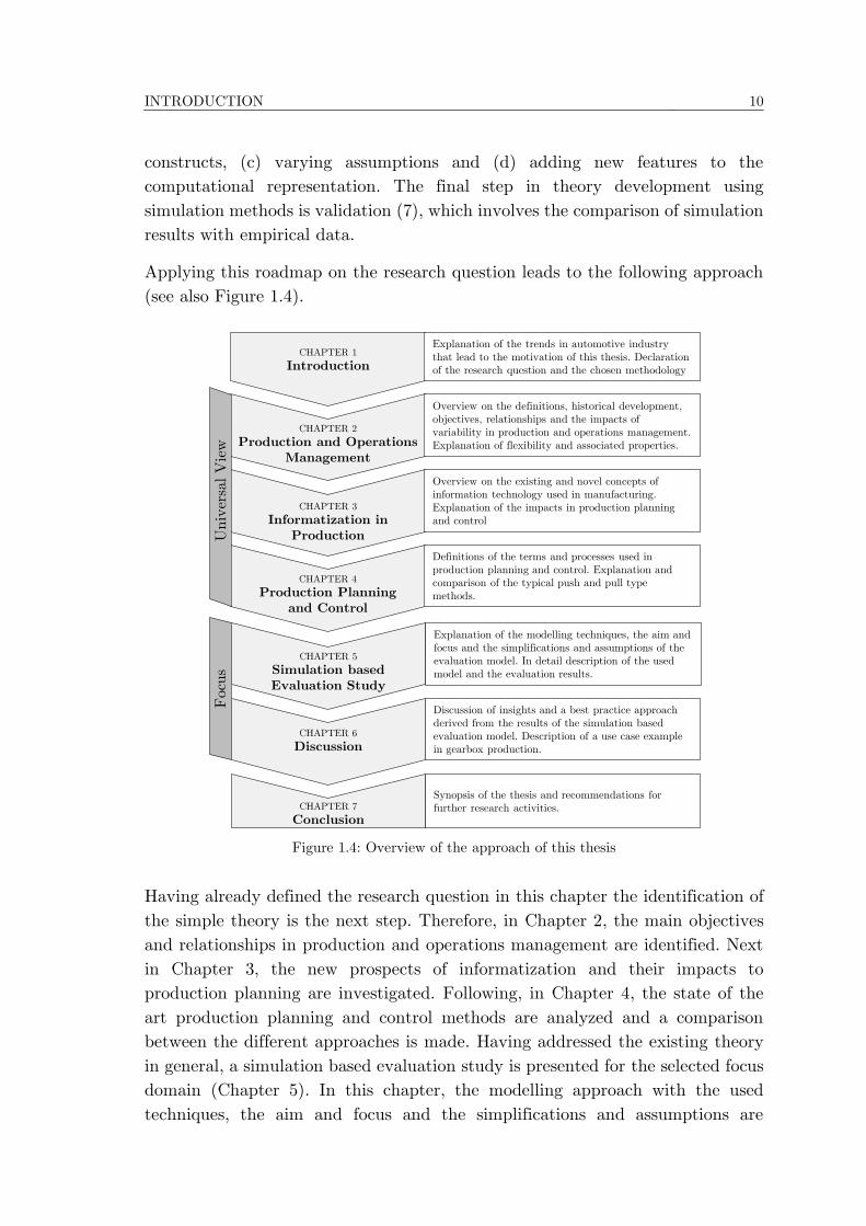
Applying this roadmap on the research question leads to the following approach
(see also Figure 1.4).
Figure 1.4: Overview of the approach of this thesis
Having already defined the research question in this chapter the identification of
the simple theory is the next step. Therefore, in Chapter 2, the main objectives
and relationships in production and operations management are identified. Next
in Chapter 3, the new prospects of informatization and their impacts to
production planning are investigated. Following, in Chapter 4, the state of the
art production planning and control methods are analyzed and a comparison
between the different approaches is made. Having addressed the existing theory
in general, a simulation based evaluation study is presented for the selected focus
domain (Chapter 5). In this chapter, the modelling approach with the used
techniques, the aim and focus and the simplifications and assumptions are
CHAPTER 2
Production and OperationsManagement
CHAPTER 1
Introduction
CHAPTER 3
Informatization inProduction
CHAPTER 4
Production Planningand Control
Overview on the definitions, historical development, objectives, relationships and the impacts of variability in production and operations management. Explanation of flexibility and associated properties.
Explanation of the trends in automotive industry that lead to the motivation of this thesis. Declaration of the research question and the chosen methodology
Overview on the existing and novel concepts of information technology used in manufacturing. Explanation of the impacts in production planning and control
Definitions of the terms and processes used in production planning and control. Explanation and comparison of the typical push and pull type methods.
Synopsis of the thesis and recommendations for further research activities.
Univ
ersa
l V
iew
Foc
us
CHAPTER 5
Simulation basedEvaluation Study
CHAPTER 6
Discussion
Explanation of the modelling techniques, the aim and focus and the simplifications and assumptions of the evaluation model. In detail description of the used model and the evaluation results.
Discussion of insights and a best practice approach derived from the results of the simulation based evaluation model. Description of a use case example in gearbox production.
CHAPTER 7
Conclusion
INTRODUCTION 11
explained. Furthermore, the implemented computational representation is
explained in-detail. Thereby the used production model, the customer model, as
well as the used planning methods get described. Also the results of the various
simulation experiments are shown in this chapter. The suggested validation of the
simulation results with empirical data is not made in this study for the following
reason: According to Davis et al. (2007) validation is less important “…if the
theory is based on empirical evidence (e.g., field—based case studies and
empirically grounded processes)” for then the theory already has some external
validation. Therefore, in the simulation model of this study no additional
validation is needed because grounded production models and planning methods
are used. The investigated novel theory is then discussed in Chapter 6.
Furthermore, a use case example in the automotive gearbox production is given
in this chapter. Finally, in the conclusion, a synopsis of the found insights and
recommendations for further research activities are given.
Production and
Operations M anagement
There is nothing so useless as doing efficiently
that which should not be done at all. Peter F. Drucker (1909 – 2005)
This chapter deals with the basic definitions and gives an overview of the
historical development of management in production. Furthermore, the ongoing
developments and hypes in this science field are discussed. Next, the strategic
objectives of an operation are explained and broken down to operational
objectives. Thereby, the conflicting operational target and the basic relationships
between them are explained. Also the different types and influences of variability
on the operational targets are shown. Based on these insights, the classical ways
to tackle variability, flexibility and its associated concepts and different structural
concepts between the various flexibility dimensions are discussed.
C H A P T E R
PRODUCTION AND OPERATIONS MANAGEMENT 13
2.1 Definitions
Definitions form the basic building blocks for each science. This chapter provides
definitions of the term “production and operations management” and also of the
term “logistics”.
2.1.1 Production and Operations Management
A manufacturing operation is characterized by tangible outputs (products) of
manufacturing conversation processes with no customer participation whereas a
service operation is characterized by intangible outputs in which customers
participate and consume immediately. Typically, service operations use more
labor and less equipment than manufacturing operations. (Kumar & Suresh, 2008)
In literature the term production and operations management (POM) is often
used for both types, manufacturing and service operations. The term production
management originates from Frederick W. Taylor9 and became accepted around
the 1930s. With the shift to the service sector in the 1970s the new name
operations management emerged (Kumar & Suresh, 2008). The American
Production and Inventory Control Society (APICS) defines POM in their
dictionary by “managing an organization’s production of goods or services” and
“managing the process of taking inputs and creating outputs” (2013).
Furthermore, operations management is defined by APICS as “the planning,
scheduling, and control of the activities that transform inputs into finished goods
and services” while production management is defined as “the planning,
scheduling, execution, and control of the process of converting inputs into finished
goods.” (2013).
POM distinguishes itself from other functions such as personnel, marketing,
finance, etc. Following are the activities which are listed under POM functions:
location of facilities, plant layouts and material handling, product design, process
design, production and planning control, quality control, materials management,
maintenance management (Kumar & Suresh, 2008). Material handling,
production planning and control, and material management can also be
summarized under the term logistics which is mainly used in German-speaking
Europe.
9 Frederick Winslow Taylor (1856 – 1915) was an American mechanical engineer who sought to improve
industrial efficiency. He was one of the first management consultants and also an athlete who competed
nationally in tennis and golf. (see also Chapter 0)
PRODUCTION AND OPERATIONS MANAGEMENT 14
2.1.2 Logistics
The literature offers a variety of definitions for to term logistics. The Encyclopedia
Britannica defines logistics as “…the organized movement of materials and,
sometimes, people.” (Encyclopedia Britannica, 2014). The Council of Logistics
Management, a trade organization based in the United States, defines logistics
as: “…the process of planning, implementing, and controlling the efficient,
effective flow and storage of goods, services, and related information from point
of origin to point of consumption for the purpose of conforming to customer
requirements.” (Encyclopedia Britannica, 2014). The term logistics is used in
literature in the United States since 1950 and in Germany since 1970. From the
time on a wide spread and rapidly growing importance can be found. Almost
every industrial company has departments or a director position for logistics and
a growing number of companies are offering logistics services. Within most of the
definitions the following common elements are included (Arnold, et al., 2003):
Logistic processes are all transport and storage processes and the
associated loading and unloading, storage and retrieval and the picking.
Logistic objects are either physical goods, in particular materials and
products in the industrial company, people or information.
A logistic system is intended to carry out a variety of logistical processes. It
has the structure of a network that consists of nodes, such as the inventory
points (storage locations), and connecting lines between the nodes, such as the
transport paths. The processes in the logistic system form a flow in the network.
The supply chain is the logistics system of an industrial company. It
encompasses the entire flow of goods from the suppliers to the company, within
the company and from there to the customer. It can be represented as a sequence
of transport, warehousing and production processes. (Arnold, et al., 2003)
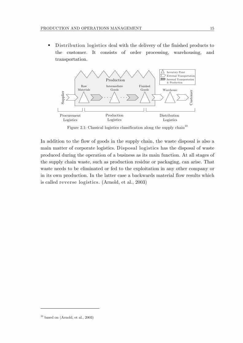
According to Arnold et al. (2003) the logistic processes along a supply chain can
be classified in the following way (see also Figure 2.1):
Procurement logistics concern the flow of goods from the supplier to
the raw material inventory point. This includes activities such as market
research, requirements planning, make-or-buy decisions, supplier
management, ordering, and order controlling.
Production logistics connect procurement to distribution logistics. Its
main function is to use available production capacities to produce the
products needed in distribution logistics. Production logistics activities are
related to organizational concepts, layout planning, production planning,
and control.
PRODUCTION AND OPERATIONS MANAGEMENT 15
Distribution logistics deal with the delivery of the finished products to
the customer. It consists of order processing, warehousing, and
transportation.
Figure 2.1: Classical logistics classification along the supply chain
10
In addition to the flow of goods in the supply chain, the waste disposal is also a
main matter of corporate logistics. Disposal logistics has the disposal of waste
produced during the operation of a business as its main function. At all stages of
the supply chain waste, such as production residue or packaging, can arise. That
waste needs to be eliminated or fed to the exploitation in any other company or
in its own production. In the latter case a backwards material flow results which
is called reverse logistics. (Arnold, et al., 2003)
10 based on (Arnold, et al., 2003)
Supplier
Cust
omer
Warehouse
FinishedGoods
IntermediateGoods
RawMaterials
. . .. . .
ProcurementLogistics
ProductionLogistics
Distribution Logistics
External Transportation
Internal Transportation& Production
Inventory Point
Production
PRODUCTION AND OPERATIONS MANAGEMENT 16
2.2 M ilestones and Hypes
This chapter deals with the history development of POM and the ongoing trends.
Similar to other science disciplines the development of POM is coined by
milestones and hypes that changed the way production management has been
done. Understanding this development is crucial to analyzing existing production
systems and finding ways to improve them.
2.2.1 Historical M ilestones
First Industrial Revolution
For time immemorial, products were made to fulfill the needs of society. In the
early days these products met on an individual basis. Prior to the first industrial
revolution, skilled craftsmen made products customized to individual needs, in
small-scale, for limited markets and labor rather than capital intensive. (Hopp &
Spearman, 2008)
In the mid-18th century several innovations appeared that helped to mechanize
many of the traditional manual operations and to perform standard tasks at a
faster and more effective pace. The single most important innovation of this first
industrial revolution, was the steam engine, developed by James Watt11 in
1765. Furthermore, Adam Smith12 proclaimed the end of the old mercantilist
system and the beginning of the modern capitalism in his Wealth of Nations
in 1776, in which he articulated the benefit of the division of labor (Hopp &
Spearman, 2008). He proposed that the production process should be broken down
into small tasks, which should be performed by different workers. Through the
work on limited repetitive tasks, the worker would specialize and productivity
will improve. According to Hopp & Spearman (2008) “…Adam Smith and James
Watt did more to change the world around them than anyone else in their period
of history”.
In 1798 Eli Whitney13 proved that the usage of interchangeable parts is a
sound industrial practice. The production of first of all firearms and then also
other goods which were custom made one at a time shifted to a volume production
11 James Watt (1736 –1819) was a Scottish inventor and mechanical engineer whose improvements to the
steam engine were fundamental to the changes brought by the Industrial Revolution. 12 Adam Smith (1723 – 1790) was a Scottish moral philosopher and a pioneer of political economy. Smith
is still among the most influential thinkers in the field of economics today. 13 Eli Whitney (1765 – 1825) was an American inventor also known for inventing the cotton gin.
PRODUCTION AND OPERATIONS MANAGEMENT 17
of standardized parts. This development also stimulated the needs for
measurements and quality inspections. (Hopp & Spearman, 2008)
The centralized power sources of the first industrial revolution also made new
organizational structures viable. At that time foreman ruled their shops,
coordinating all of the activities needed for the limited number of products for
which they were responsible. Production planning and control also started simple.
According to Herrmann (2006) “Schedules, when used at all, listed only when
work on an order should begin or when the order is due. They didn’t provide any
information about how long the total order should take or about the time required
for the individual operations”.
Second Industrial Revolution
Throughout the 1800s, there were many technological advances, but management
theory and practice were almost non-existent. In the USA the build of the
railroads ignited the second industrial revolution for the following three reasons.
First for the complex operations required large-scale management hierarchies and
modern accounting practices. Second, their construction created a large market
for mass-production products and third, they connected the country with an all-
weather transportation. Also, other industries followed the trend of the railroads
towards big-business through horizontal and vertical integration. This made the
USA to the land of big business by the beginning of the 20th century. M ass
production of mechanical products based on new methods for fabrication and
assembly of interchangeable parts was full in swing, but it remained for Henry
Ford14 to enable the high-speed mass production of complex mechanical products
with his innovation of the moving assembly line. (Hopp & Spearman, 2008)
Ford recognized the importance of throughput velocity and sought to bring the
products to the worker in a nonstop, continuous stream.
The thing is to keep everting in motion and take the work to the
man and not the man to the work. That is the real principle of
our production, and conveyors are only one of many means to
an end. (Ford, 1926)
Ford focused on continual improvement of a single model and pushed the mass
production to new limits. He believed in a perfectible product and never valued
the need of bringing new products to the market. His famous statement that “the
14 Henry Ford (1863 –1947) was an American industrialist, the founder of the Ford Motor Company, and
sponsor of the development of the assembly line technique of mass production, which he successfully
applied in the production of the famous car Model T.
PRODUCTION AND OPERATIONS MANAGEMENT 18
customer can have any color as long as it’s black” also shows that (Ford, 1926).
Ford failed to see the potential of producing a variety of end products from a
common set of standardized parts. His focus on speed motivated his moving
assembly line but his concern was even far beyond assembly. Ford claimed that
“Our finished inventory is all in transit. So is most of our raw material inventory”
(1926). His company could take ore from a mine and produce a car in only 81
hours. Moreover, Ford used many methods of the newly emerging discipline of
scientific management. (Hopp & Spearman, 2004)
Scientific M anagement
In the early 1900s, Frederick W. Taylor15 propounded the concept of scientific
management. As Whitney had made standardized material units and made
them interchangeable, Taylor tried to do the same for work units by applying
work standards. According to Drucker (1954) Taylor’s system “…may well be the
most powerful as well as the most lasting contribution America has made to
Western through since the Federalist Paper.”.
He maintained that there was a best method of performing a task which could be
identified through observation, measurement and analysis. He was of the view
that workers must perform tasks in a specified manner in order to improve
productivity and standards must be laid down for the amount of work to be
performed in a day. His philosophy assumed that workers are motivated by
economic considerations and economic incentives such as different rates of pay.
Beside time studies and incentive systems Taylor proposed also a system of
functional foremanship in which the traditional single foreman is replaced by
different supervisors, each responsible for different specific function such as
quality of work, machine setup, machine speeds, maintenance, routing, scheduling
and also time recording. (Hopp & Spearman, 2008)
Taylor’s biggest contribution to POM was the clear separation of the jobs of
management who should do the planning, from those of the workers who should
work. He even placed the activities of planning and doing in entirely separated
jobs. All planning activities rested within the management, while workers were
expected to carry out their task in the manner determined by the management
(Hopp & Spearman, 2008). However, such a removal of the responsibility from
the workers causes a negative effect on quality (Juran, 1992). Furthermore,
15 Frederick Winslow Taylor (1856 –1915) was an American mechanical engineer who sought to improve
industrial efficiency. He was one of the first management consultants and also an athlete who competed
nationally in tennis and golf.
PRODUCTION AND OPERATIONS MANAGEMENT 19
Taylor’s reduction of work task to their simplest components could cause negative
effects on the productivity on the long time and make workers inflexible. In
contrast the Japanese, with their holistic perspective, quality circles, suggestion
programs and worker empowerment practices legalize planning on the part of the
worker and encourage their workforce to be more flexible.
One of Taylor’s collaborators was Henry L. Gantt16, who created innovative
charts for production control. According to APICS, a Gantt chart is “the earliest
and best known type of control chart especially designed to show graphically the
relationship between planned production and actual performance.” (2013).
Gantt (1919) gives two principles for his charts, which are still used by modern
project management software:
Measure activities by the amount of time needed to complete them
The space on the chart can be used to represent the amount of the activity
that should have been done in that time
He described several different types of charts on which Clark (1942) provides an
excellent overview. The so called daily balance of work shows the amount of work
to be done and the amount that is done and serves as a method of scheduling.
Gantt’s man’s record and machine record charts are used to record past’s
performance and also track reasons for inefficiency. Beside those he also developed
layout charts, progress charts, schedule charts, order charts and so on. In
conclusion it can be said that Gantt was a pioneer in developing graphical ways
to visualize schedules and shop status (Herrmann, 2006).
Beside Taylor and Gantt there were also other pioneers of scientific management.
The most prominent among these were Frank17 and Lillian Gilbreth18. They
extended Taylors time study to what they called motion study, in which they
made detailed analysis of motion involving bricklaying in the search of a more
effective procedure. They were also the first that applied motion picture cameras
for analyzing human motions, which they categorized into 18 basic components.
(Hopp & Spearman, 2008)
16 Henry Laurence Gantt (1861 – 1919) was an American mechanical engineer and management consultant
who is best known for developing the Gantt chart in the 1910s. 17 Frank Bunker Gilbreth (1868 – 1924) was an American early advocate of scientific management and a
pioneer of motion study. He is also known as the father in the book Cheaper by the Dozen and Belles
which tells the story of their family life with their twelve children, and describes how they applied their
interest in time and motion study to the organization and daily activities of such a large family. 18 Lillian Evelyn Moller Gilbreth (1878 – 1972) was an American psychologist and industrial engineer. She
was together with her husband efficiency experts who contributed to the study of industrial engineering
in fields such as motion study and human factors.
PRODUCTION AND OPERATIONS MANAGEMENT 20
Organization and M anagement Science
In the interwar period family control of large-scale, vertically integrated
manufacturing enterprises was still common. Further organizational growth
would require the development of institutional structures and management
procedures for controlling the resulting organizations to take advantage of the
economy of scope. (Hopp & Spearman, 2008)
This period was strongly influenced by Pierre S. Du Pont19, who was well aware
of scientific management principles. Together with his associates, they installed
Taylor’s manufacturing control techniques and accounting system and also
introduced psychological testing for personal selection. His most influencing
innovation was the refined use of return on investment (ROI) to evaluate the
performance of departments. (Hopp & Spearman, 2008)
Together with Alfred P. Sloan20 at General Motors, they planned to structure the
company as a collection of autonomous operation division coordinated but not
run by a strong general office. The various divisions were carefully targeted at
specific market in accordance with Sloan’s goal of “a car for every purse and
purpose” (1924). This strategy was stunningly effective, while Ford was still
producing the Model T. Together Sloan and Du Pont shaped the structure of
modern manufacturing organization. Even today, companies with a single line of
product for a single market use a centralized, function department organization,
while companies with several product lines or markets use the multidivisional,
decentralized structure developed at General Motors. (Hopp & Spearman,
2008)
This period also saw the development of the human relation movement. Elton
Mayo carried out the famous Hawthorn studies and concluded that productivity
was not affected by the environment alone (Hopp & Spearman, 2008). Worker
motivation has an important part to play which lead to the development of
motivation theories by Maslow21, Herzberg22, McGregor23 and others.
19 Pierre Samuel Du Pont (1870 – 1954) was an American entrepreneur and was president of General
Motors from 1915-1920. 20 Alfred Pritchard Sloan (1875 – 1966) was an American business executive. He was a long-time president,
chairman, and CEO of General Motors. 21 Abraham Harold Maslow (1908 – 1970) was an American psychologist who was best known for creating
Maslow's hierarchy of needs, a theory of psychological health predicated on fulfilling innate human needs
in priority, culminating in self-actualization. 22 Frederick Irving Herzberg (1923 – 2000) was an American psychologist is most famous for introducing
job enrichment and the Motivator-Hygiene theory. 23 Douglas Murray McGregor (1906 – 1964) was an American management professor and is best known for
his Theory X and Theory Y.
PRODUCTION AND OPERATIONS MANAGEMENT 21
2.2.2 Recent Developments
The recent developments in POM were mainly influenced by the emerging
possibilities of information technology and Japanese management practices. These
period is also characterized by the different perspectives on problem solving of
Western and Far East societies.
Western societies favored the reductionist method to analyze systems by breaking
them down into their component parts and studying each one individually. In
contrast, Far Eastern societies had a more holistic or system perspective in which
the individual components are viewed much more in terms of their interactions
with other subsystem in the perspective of the overall goal. A major contribution
of the Western world to POM was created during World War II with the new
emerged science discipline Operations Research (OR). This discipline
developed several quantitative techniques such as linear programming, inventory
control methods, queuing theory and simulation techniques which lead among
others to the development of mathematical models for determining “optimal” lot
sizes based on setup and inventory holding costs. In contrast, the Japanese,
analyzed manufacturing systems in a more holistic sense and focused not on the
optimization of lot sizes for given setup times. Rather, they did not see the setup
times as constant and recognized the, from a system perspective, clear benefit in
reducing these times. (Hopp & Spearman, 2008)
In the 1960s the primarily manufacturing competition was on cost, which resulted
in a product-focused manufacturing strategy based on high-volume production
and cost minimization. Reorder point systems (ROP) were used for production
control followed by computerized inventory control system and material
requirements planning (MRP) systems in the 1970s. At that time the Japanese
just-in-time (JIT) system also boosted this efficiency trend. In the 1980s the
primary competition changed to quality again under the Japanese influence of
total quality management (TQM). While external quality, which is everything
what the customer can see, was always of concern, the main attention was now
on the internal quality of each process step and its influence to customer
satisfaction. While costs and quality remained crucial, the 1990s were dominated
by the time based competition. The rapid development of new products
together with fast customer delivery were the new demanded abilities. (Hopp &
Spearman, 2008)
A more detailed explanation of these movements, especially the associated
developments in production planning and control systems, can be found in
Chapter 4.4.
PRODUCTION AND OPERATIONS MANAGEMENT 22
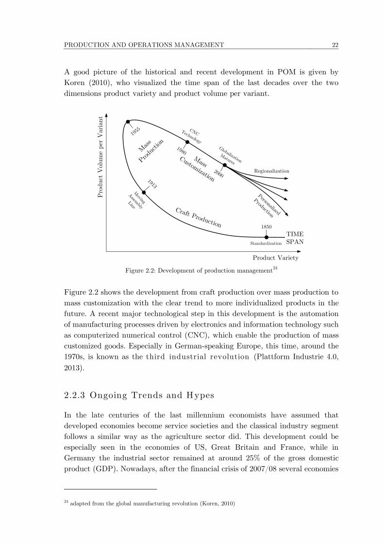
A good picture of the historical and recent development in POM is given by
Koren (2010), who visualized the time span of the last decades over the two
dimensions product variety and product volume per variant.
Figure 2.2: Development of production management
24
Figure 2.2 shows the development from craft production over mass production to
mass customization with the clear trend to more individualized products in the
future. A recent major technological step in this development is the automation
of manufacturing processes driven by electronics and information technology such
as computerized numerical control (CNC), which enable the production of mass
customized goods. Especially in German-speaking Europe, this time, around the
1970s, is known as the third industrial revolution (Plattform Industrie 4.0,
2013).
2.2.3 Ongoing Trends and Hypes
In the late centuries of the last millennium economists have assumed that
developed economies become service societies and the classical industry segment
follows a similar way as the agriculture sector did. This development could be
especially seen in the economies of US, Great Britain and France, while in
Germany the industrial sector remained at around 25% of the gross domestic
product (GDP). Nowadays, after the financial crisis of 2007/08 several economies
24 adapted from the global manufacturing revolution (Koren, 2010)
Product Variety
Pro
duct
Vol
um
e per
Vari
ant
Regionalization
1850
TIMESPANStandardization
PRODUCTION AND OPERATIONS MANAGEMENT 23
changed their views and recognized that developed economies need a strong
industrial sector to be successful due to the following reasons: First, the
productivity contribution of the industrial sector on the economy of a country. In
service industry no significant productivity increases are often possible because of
the direct interaction of people. Only with productivity improvement in the
industry sector, significant growth of the economy of a country is possible. The
second reason is the huge innovation contribution of the industrial sector. If the
production industry is outsourced to other countries also research and
development activities would follow. Third is the export contribution of the
industrial sector which has positive effects on the trade balance of an economy.
(Bauernhansl, 2014)
Due to these reasons, several developed economies initialized programs to
revitalize their industrial sector. Great Britain started the High Value
Manufacturing (TSB, 2012) program, the USA the Advanced Manufacturing
Partnership (PCAST, 2012) and the European Union is focusing its research and
development programs in HORIZON 2020 mainly on projects with high industrial
application aspects. The German federal government even called out the fourth
industrial revolution (Industry 4.0) with the aim to strengthen the production
of Germany driven by Internet of Things and cyber physical system (Plattform
Industrie 4.0, 2013). A more detailed explanation of these concepts and the
associated enabling technologies can be found in Chapter 3.2.
In the USA a similar research initiative called industrial internet is aiming to
bring the internet to the shop floor. Instead of the fourth revolution in
manufacturing the computation of time is different in the USA. The industrial
internet consortium is counting in waves in which the first wave was in general
the industrial revolution followed by the internet revolution. The industrial
internet is thereby seen as the third wave which will enable intelligent connected
machines, advanced analytics and connected people at work (Evans &
Annunziata, 2012). In logistics, the Physical Internet Initiative was founded to
develop open system, interfaces and protocols that use Internet of Things
technology in logistic systems (Montreuil, 2012).
However, beside the promising benefits of the concepts, these current trends can
also be dangerous. The vocabulary of POM is coined by buzzwords which are
often associated to a much lauded guru (Micklethwait & Wooldridge, 1996). Using
these, in the past often three letter acronym (e.g. MRP, JIT, ERP), buzzwords
and manufacturing firms have become flooded with waves of revolutions in recent
years and Industry 4.0 is only the next one. According to Hopp & Spearman such
revolutions have always “…swept through the manufacturing community,
accompanied by soaring rhetoric and passionate emotion, but with little concrete

PRODUCTION AND OPERATIONS MANAGEMENT 24
detail” (2008). However, those revolutions can be dangerous for managers to
become attached to trendy buzzwords and losing sight of their fundamental
objectives. Beside the lack of precise definition of the underlying concept
especially in practitioner literature (see Hopp & Spearman, 2003) the firm belief,
nearly on a religious level, in these buzzwords has even further drawbacks. Often
the underlying concepts behind trendy buzzwords offer only a single solution for
all situations which is especially in situations of volatile markets where flexibility
is needed by far too little (Hopp & Spearman, 2008).
PRODUCTION AND OPERATIONS MANAGEMENT 25
2.3 Objectives and Relationships
2.3.1 Strategic and Operational Objectives
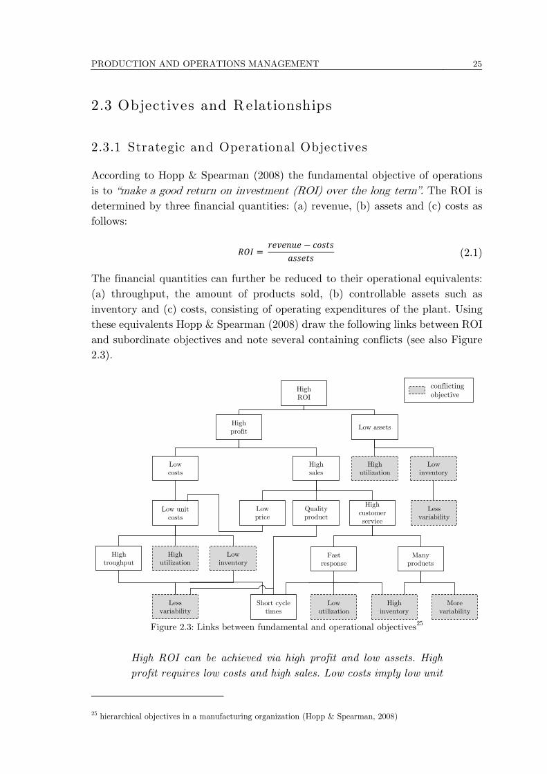
According to Hopp & Spearman (2008) the fundamental objective of operations
is to “make a good return on investment (ROI) over the long term”. The ROI is
determined by three financial quantities: (a) revenue, (b) assets and (c) costs as
follows:
𝑅𝑂𝐼 = 𝑟𝑒𝑣𝑒𝑛𝑢𝑒 − 𝑐𝑜𝑠𝑡𝑠
𝑎𝑠𝑠𝑒𝑡𝑠 (2.1)
The financial quantities can further be reduced to their operational equivalents:
(a) throughput, the amount of products sold, (b) controllable assets such as
inventory and (c) costs, consisting of operating expenditures of the plant. Using
these equivalents Hopp & Spearman (2008) draw the following links between ROI
and subordinate objectives and note several containing conflicts (see also Figure
2.3).
Figure 2.3: Links between fundamental and operational objectives
25
High ROI can be achieved via high profit and low assets. High
profit requires low costs and high sales. Low costs imply low unit
25 hierarchical objectives in a manufacturing organization (Hopp & Spearman, 2008)
HighROI
High profit
Low assets
Lowcosts
Highsales
Low unitcosts
Low price
Quality product
High customerservice
Lessvariability
High utilization
Low inventory
High troughput
High utilization
Low inventory
Fast response
Manyproducts
Lessvariability
Short cycletimes
Low utilization
High inventory
More variability
conflicting objective
PRODUCTION AND OPERATIONS MANAGEMENT 26
costs, which requires high throughput, high utilization and low
inventory… Achieving low inventory while keeping throughput
and utilization high requires variability in production to be kept
low. High sales require a high-quality product that people want to
buy, plus good customer service. High customer service requires
fast and reliable response. Fast response requires short cycle
times, low utilization and/or high inventory levels. To keep many
products available requires high inventory levels and more
(product) variability. However, to obtain high quality, we need
less (process) variability and short cycle times (to facilitate rapid
defect detection). Finally, on the assets side of the hierarchy, we
need high utilization to minimize investment in capital equipment
and low inventory in order to reduce money tied up in stock. As
noted above, the combination of low inventory and high utilization
requires low variability. (Hopp & Spearman, 2008)
One conflict in this hierarchy is, for instance, on the one hand the need of high
inventory for fast response, but on the other hand the demand of low inventory
to keep total assets low. These conflicting objectives result in that the
improvement of one operational target usually leads to a decline in another target
dimension. This target contradiction is known in the literature by Gutenberg
(1951) as the dilemma of operations planning which describes the conflict of
interests between the maximization of delivery reliability and utilization and the
minimization of inventory and consequentially lead time.
Nevertheless, fundamental relationships between the conflicting operational
targets exist.
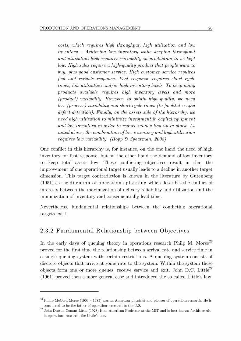
2.3.2 Fundamental Relationship between Objectives
In the early days of queuing theory in operations research Philp M. Morse26
proved for the first time the relationship between arrival rate and service time in
a single queuing system with certain restrictions. A queuing system consists of
discrete objects that arrive at some rate to the system. Within the system these
objects form one or more queues, receive service and exit. John D.C. Little27
(1961) proved then a more general case and introduced the so called Little’s law.
26 Philip McCord Morse (1903 – 1985) was an American physicist and pioneer of operations research. He is
considered to be the father of operations research in the U.S. 27 John Dutton Conant Little (1928) is an American Professor at the MIT and is best known for his result
in operations research, the Little’s law.
PRODUCTION AND OPERATIONS MANAGEMENT 27
𝐿 = 𝜆 × 𝑊
𝐿 = 𝑎𝑣𝑒𝑟𝑎𝑔𝑒 𝑛𝑢𝑚𝑏𝑒𝑟 𝑜𝑓 𝑖𝑡𝑒𝑚𝑠 𝑖𝑛 𝑡ℎ𝑒 𝑞𝑢𝑒𝑢𝑖𝑛𝑔 𝑠𝑦𝑠𝑡𝑒𝑚 𝑊 = 𝑎𝑣𝑒𝑟𝑎𝑔𝑒 𝑤𝑎𝑖𝑡𝑖𝑛𝑔 𝑡𝑖𝑚𝑒 𝑖𝑛 𝑡ℎ𝑒 𝑠𝑦𝑠𝑡𝑒𝑚 𝑓𝑜𝑟 𝑎𝑛 𝑖𝑡𝑒𝑚
𝜆 = 𝑎𝑣𝑒𝑟𝑎𝑔𝑒 𝑛𝑢𝑚𝑏𝑒𝑟 𝑜𝑓 𝑖𝑡𝑒𝑚𝑠 𝑎𝑟𝑟𝑖𝑣𝑖𝑛𝑔 𝑝𝑒𝑟 𝑢𝑛𝑖𝑡 𝑡𝑖𝑚𝑒
(2.2)
The Little’s law says that under steady state conditions, the average number of
items in a queuing system 𝐿 equals the average rate at which items arrive 𝑊
multiplied by the average time that an item spends in the system 𝜆. This
relationship is remarkably simple and general as it is not mentioned how many
servers there are, whether each server has its own queue or a single queue for all
servers, what the service time distribution are, or on what distribution of inter-
arrival times, etc. (Little & Graves, 2008)
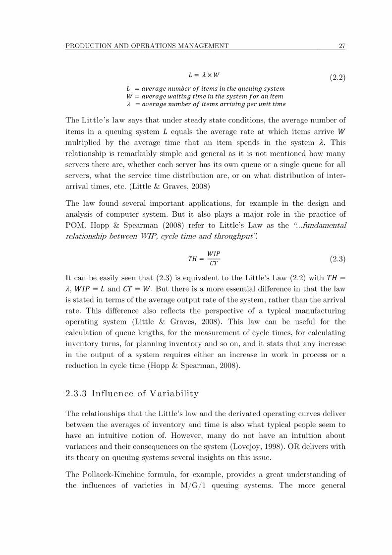
The law found several important applications, for example in the design and
analysis of computer system. But it also plays a major role in the practice of
POM. Hopp & Spearman (2008) refer to Little’s Law as the “…fundamental
relationship between WIP, cycle time and throughput”.
𝑇𝐻 = 𝑊𝐼𝑃
𝐶𝑇 (2.3)
It can be easily seen that (2.3) is equivalent to the Little’s Law (2.2) with 𝑇𝐻 =
𝜆, 𝑊𝐼𝑃 = 𝐿 and 𝐶𝑇 = 𝑊. But there is a more essential difference in that the law
is stated in terms of the average output rate of the system, rather than the arrival
rate. This difference also reflects the perspective of a typical manufacturing
operating system (Little & Graves, 2008). This law can be useful for the
calculation of queue lengths, for the measurement of cycle times, for calculating
inventory turns, for planning inventory and so on, and it stats that any increase
in the output of a system requires either an increase in work in process or a
reduction in cycle time (Hopp & Spearman, 2008).
2.3.3 Influence of Variability
The relationships that the Little’s law and the derivated operating curves deliver
between the averages of inventory and time is also what typical people seem to
have an intuitive notion of. However, many do not have an intuition about
variances and their consequences on the system (Lovejoy, 1998). OR delivers with
its theory on queuing systems several insights on this issue.
The Pollacek-Kinchine formula, for example, provides a great understanding of
the influences of varieties in M/G/1 queuing systems. The more general
PRODUCTION AND OPERATIONS MANAGEMENT 28
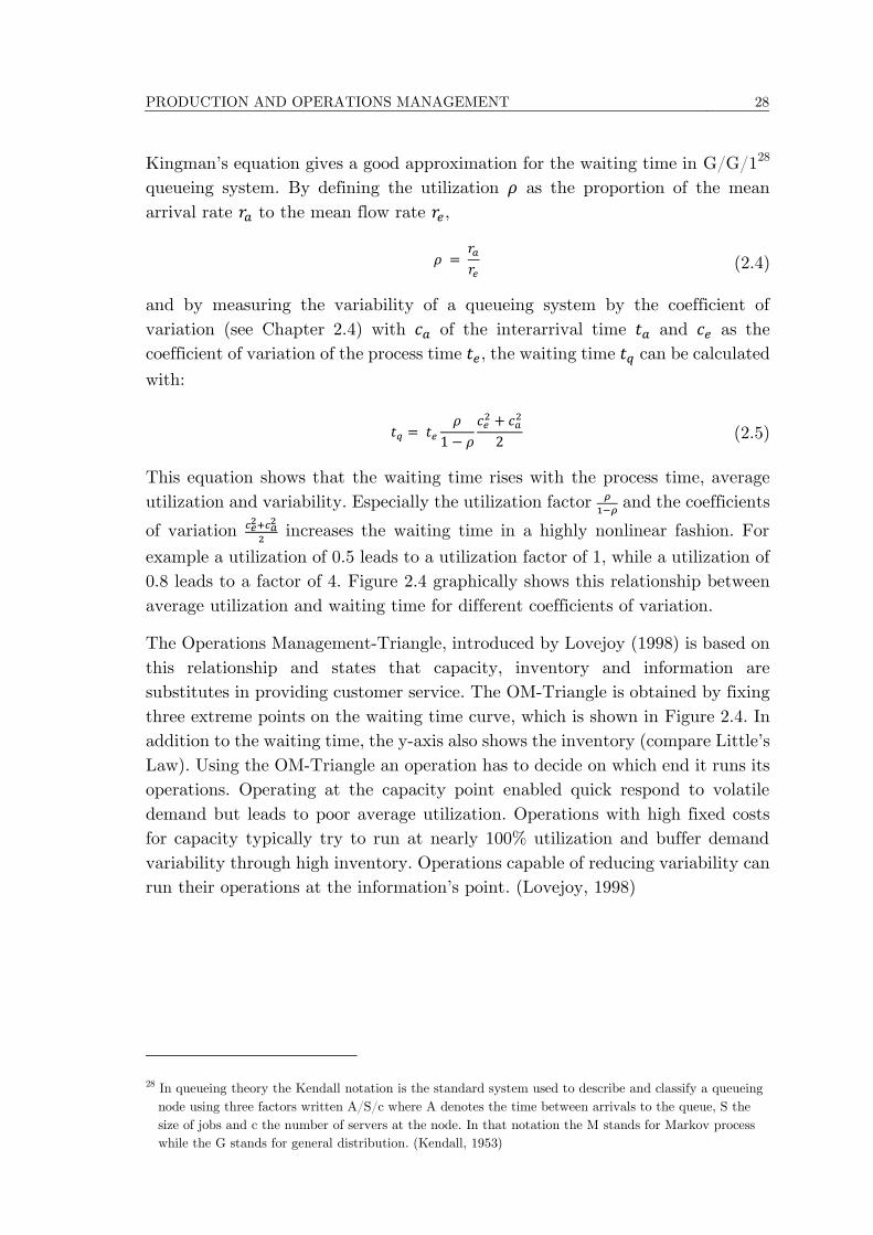
Kingman’s equation gives a good approximation for the waiting time in G/G/128
queueing system. By defining the utilization 𝜌 as the proportion of the mean
arrival rate 𝑟𝑎 to the mean flow rate 𝑟𝑒,
𝜌 = 𝑟𝑎
𝑟𝑒
(2.4)
and by measuring the variability of a queueing system by the coefficient of
variation (see Chapter 2.4) with 𝑐𝑎 of the interarrival time 𝑡𝑎 and 𝑐𝑒 as the
coefficient of variation of the process time 𝑡𝑒, the waiting time 𝑡𝑞 can be calculated
with:
𝑡𝑞 = 𝑡𝑒
𝜌
1 − 𝜌
𝑐𝑒2 + 𝑐𝑎
2
2 (2.5)
This equation shows that the waiting time rises with the process time, average
utilization and variability. Especially the utilization factor 𝜌
1−𝜌 and the coefficients
of variation 𝑐𝑒2+𝑐𝑎
2
2 increases the waiting time in a highly nonlinear fashion. For
example a utilization of 0.5 leads to a utilization factor of 1, while a utilization of
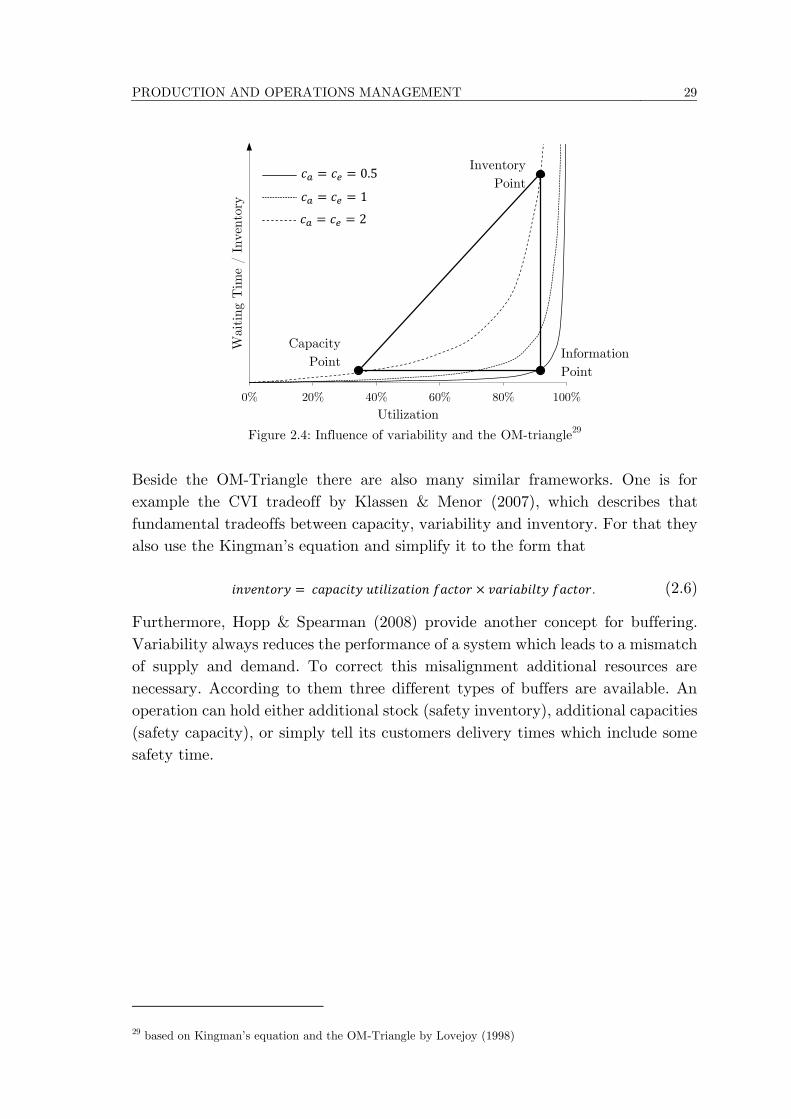
0.8 leads to a factor of 4. Figure 2.4 graphically shows this relationship between
average utilization and waiting time for different coefficients of variation.
The Operations Management-Triangle, introduced by Lovejoy (1998) is based on
this relationship and states that capacity, inventory and information are
substitutes in providing customer service. The OM-Triangle is obtained by fixing
three extreme points on the waiting time curve, which is shown in Figure 2.4. In
addition to the waiting time, the y-axis also shows the inventory (compare Little’s
Law). Using the OM-Triangle an operation has to decide on which end it runs its
operations. Operating at the capacity point enabled quick respond to volatile
demand but leads to poor average utilization. Operations with high fixed costs
for capacity typically try to run at nearly 100% utilization and buffer demand
variability through high inventory. Operations capable of reducing variability can
run their operations at the information’s point. (Lovejoy, 1998)
28 In queueing theory the Kendall notation is the standard system used to describe and classify a queueing
node using three factors written A/S/c where A denotes the time between arrivals to the queue, S the
size of jobs and c the number of servers at the node. In that notation the M stands for Markov process
while the G stands for general distribution. (Kendall, 1953)
PRODUCTION AND OPERATIONS MANAGEMENT 29
Figure 2.4: Influence of variability and the OM-triangle
29
Beside the OM-Triangle there are also many similar frameworks. One is for
example the CVI tradeoff by Klassen & Menor (2007), which describes that
fundamental tradeoffs between capacity, variability and inventory. For that they
also use the Kingman’s equation and simplify it to the form that
𝑖𝑛𝑣𝑒𝑛𝑡𝑜𝑟𝑦 = 𝑐𝑎𝑝𝑎𝑐𝑖𝑡𝑦 𝑢𝑡𝑖𝑙𝑖𝑧𝑎𝑡𝑖𝑜𝑛 𝑓𝑎𝑐𝑡𝑜𝑟 × 𝑣𝑎𝑟𝑖𝑎𝑏𝑖𝑙𝑡𝑦 𝑓𝑎𝑐𝑡𝑜𝑟. (2.6)
Furthermore, Hopp & Spearman (2008) provide another concept for buffering.
Variability always reduces the performance of a system which leads to a mismatch
of supply and demand. To correct this misalignment additional resources are
necessary. According to them three different types of buffers are available. An
operation can hold either additional stock (safety inventory), additional capacities
(safety capacity), or simply tell its customers delivery times which include some
safety time.
29 based on Kingman’s equation and the OM-Triangle by Lovejoy (1998)
0% 20% 40% 60% 80% 100%
wai
ting t
ime
/ in
vento
ry
utilization0% 20% 40% 60% 80% 100%
Waitin
g T
ime
/ In
ven
tory
Utilization
Inventory
Point
Capacity
PointInformation
Point
PRODUCTION AND OPERATIONS MANAGEMENT 30
2.4 Variability
As the previous chapter already showed that variability always degrade the
performance of an operating system or how Hopp & Spearman (2008) wrote “…the
corrupting influence of variability”, this chapter gives an overview of definitions
and classifications of variability to better understand its causes.
2.4.1 Definitions
First of all the definition of the terms certainty, uncertainty, risk and variability
must be clarified. Since we know from Heisenberg’s principle of uncertainty30 the
world we live in is not deterministic. Also chaos theory shows that even a
deterministic system can be sufficiently complex and cannot be completely
predicted.
One possible definition on certainty, uncertainty and risk is coming from
decision theory. In one of the most influential textbooks in decision theory by
Luce & Raiffa (1957) the terms are defined as follows:
We shall say that we are in the realm of decision making under:
(a) Certainty if each action is known to lead invariably to a
specific outcome. ...
(b) Risk if each action leads to one of a set of possible specific
outcomes, each outcome occurring with a known probability. The
probabilities are assumed to be known to the decision maker. …
(c) Uncertainty if either action or both has as its consequence a
set of possible specific outcomes, but where the probabilities of
these outcomes are completely unknown or are not even
meaningful. (Luce & Raiffa, 1957)
So while risk can be estimated, as it is a function of outcome and probability, it
is not possible to estimate the outcome or the probability of its occurrence for
uncertainty.
When it comes to decisions, intuition also plays an important role, however
intuition is typically acting as if the world would be deterministic, without any
randomness. In mathematics a quantitative measure of the shape of a set of points
are the so called moments. While the first moment is the mean value of the points,
the second describes the variance. In addition the shape is also described by the
30 is principle in quantum mechanics which stats that it is not possible to simultaneously arbitrarily
determined precisely two complementary variables from
PRODUCTION AND OPERATIONS MANAGEMENT 31
third (skewness), the fourth (kurtosis) and higher moments. Our intuition tends
to be much less developed for second or higher moments. Therefore, random
phenomena get often misinterpreted (Hopp & Spearman, 2008). In statistics the
regression toward the mean31 describes such a phenomena. Also psychology deals
with problems due to randomness. For example Paul Watzlawick32 (1987)
mentions in that respect so called noncontingent reward experiment33 in which
experimental subjects in the end always format of a hypothesis of the relationship
between two independent random numbers.
As already mentioned several times before, variability is in POM an often used
term for the randomness in processes. A formal definition of variability is the
“quality of nonuniformity of a class of entities” (Hopp & Spearman, 2008). A
measure for variability of a random variable is the coefficient of variation 𝑐𝑣,
which is the standard deviation 𝜎 divided by the mean 𝜇.
𝑐𝑣 = 𝜎
𝜇 (2.7)
When talking about variability Hopp & Spearman (2008) distinguish between two
main types: controllable variability, which arises directly from decisions (e.g.
batch size, amount of products) and random variability, which arises from events
beyond immediate control (e.g. customer demand, machine breakdown). Klassen
& Menor (2007) suggest another typology shown in Table 2.1. They use the
dimensions’ form and source to classify the variability of a system. In the
dimension form a distinction between random and predictable variability and in
the dimension source a distinction between internal (i.e. process) and external
(i.e. supply chain) origin is made.
31 Regression toward the mean is the phenomenon that if a variable is extreme on its first measurement, it
will tend to be closer to the average on its second measurement - and, paradoxically, if it is extreme on
its second measurement, it will tend to have been closer to the average on its first. 32 Paul Watzlawick (1921 – 2007) was an Austrian family therapist, psychologist, communications theorist,
and philosopher. His most prominent insight is that “one cannot not communicate”. 33 Subjects get presented a pairs of numbers. They have to decide whether the numbers match or not. The
pairs of numbers are collected at random, and the experimenter gives his appraisal right or wrong on the
basis of half rising Gaussian bell curve. The rating right is continuous with the experiment more and
more frequently, leading to the formation of a hypothesis by the subject.
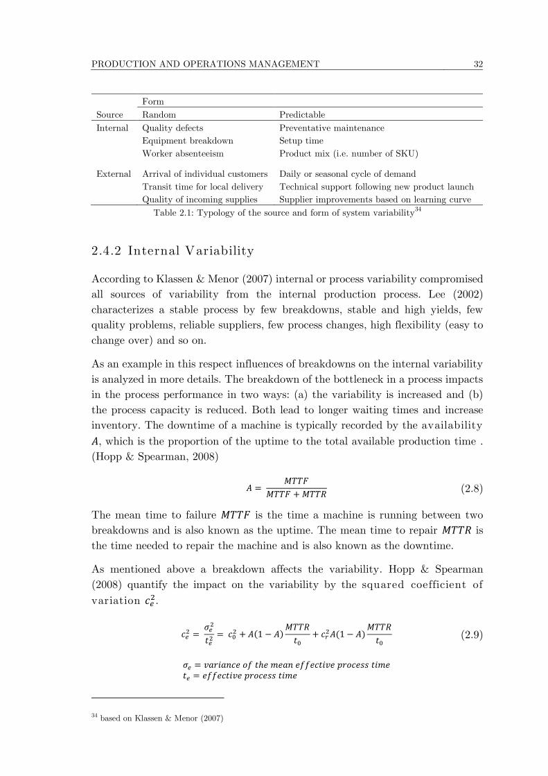
PRODUCTION AND OPERATIONS MANAGEMENT 32
Form
Source Random Predictable
Internal
Quality defects
Equipment breakdown
Worker absenteeism
Preventative maintenance
Setup time
Product mix (i.e. number of SKU)
External
Arrival of individual customers
Transit time for local delivery
Quality of incoming supplies
Daily or seasonal cycle of demand
Technical support following new product launch
Supplier improvements based on learning curve
Table 2.1: Typology of the source and form of system variability34
2.4.2 Internal Variability
According to Klassen & Menor (2007) internal or process variability compromised
all sources of variability from the internal production process. Lee (2002)
characterizes a stable process by few breakdowns, stable and high yields, few
quality problems, reliable suppliers, few process changes, high flexibility (easy to
change over) and so on.
As an example in this respect influences of breakdowns on the internal variability
is analyzed in more details. The breakdown of the bottleneck in a process impacts
in the process performance in two ways: (a) the variability is increased and (b)
the process capacity is reduced. Both lead to longer waiting times and increase
inventory. The downtime of a machine is typically recorded by the availability
𝐴, which is the proportion of the uptime to the total available production time .
(Hopp & Spearman, 2008)
𝐴 = 𝑀𝑇𝑇𝐹
𝑀𝑇𝑇𝐹 + 𝑀𝑇𝑇𝑅 (2.8)
The mean time to failure 𝑀𝑇𝑇𝐹 is the time a machine is running between two
breakdowns and is also known as the uptime. The mean time to repair 𝑀𝑇𝑇𝑅 is
the time needed to repair the machine and is also known as the downtime.
As mentioned above a breakdown affects the variability. Hopp & Spearman
(2008) quantify the impact on the variability by the squared coefficient of
variation 𝑐𝑒2.
𝑐𝑒2 =
𝜎𝑒2
𝑡𝑒2
= 𝑐02 + 𝐴(1 − 𝐴)
𝑀𝑇𝑇𝑅
𝑡0
+ 𝑐𝑟2𝐴(1 − 𝐴)
𝑀𝑇𝑇𝑅
𝑡0
(2.9)
𝜎𝑒 = 𝑣𝑎𝑟𝑖𝑎𝑛𝑐𝑒 𝑜𝑓 𝑡ℎ𝑒 𝑚𝑒𝑎𝑛 𝑒𝑓𝑓𝑒𝑐𝑡𝑖𝑣𝑒 𝑝𝑟𝑜𝑐𝑒𝑠𝑠 𝑡𝑖𝑚𝑒 𝑡𝑒 = 𝑒𝑓𝑓𝑒𝑐𝑡𝑖𝑣𝑒 𝑝𝑟𝑜𝑐𝑒𝑠𝑠 𝑡𝑖𝑚𝑒
34 based on Klassen & Menor (2007)
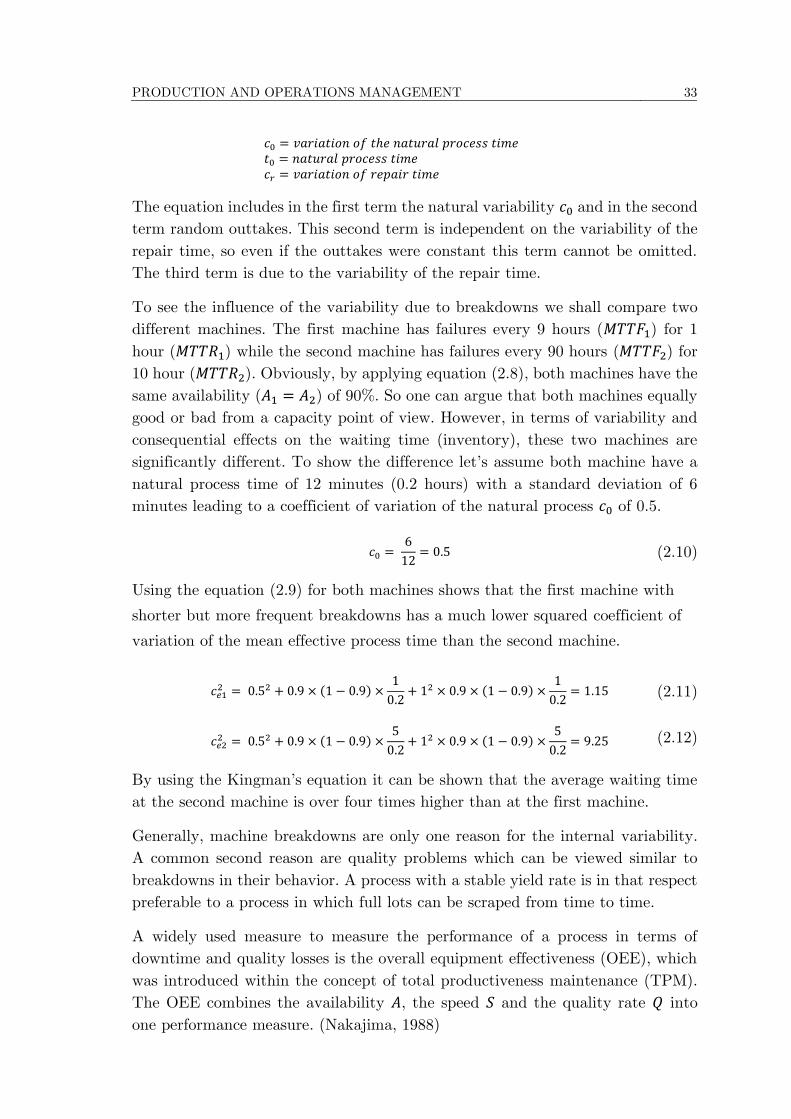
PRODUCTION AND OPERATIONS MANAGEMENT 33
𝑐0 = 𝑣𝑎𝑟𝑖𝑎𝑡𝑖𝑜𝑛 𝑜𝑓 𝑡ℎ𝑒 𝑛𝑎𝑡𝑢𝑟𝑎𝑙 𝑝𝑟𝑜𝑐𝑒𝑠𝑠 𝑡𝑖𝑚𝑒 𝑡0 = 𝑛𝑎𝑡𝑢𝑟𝑎𝑙 𝑝𝑟𝑜𝑐𝑒𝑠𝑠 𝑡𝑖𝑚𝑒 𝑐𝑟 = 𝑣𝑎𝑟𝑖𝑎𝑡𝑖𝑜𝑛 𝑜𝑓 𝑟𝑒𝑝𝑎𝑖𝑟 𝑡𝑖𝑚𝑒
The equation includes in the first term the natural variability 𝑐0 and in the second
term random outtakes. This second term is independent on the variability of the
repair time, so even if the outtakes were constant this term cannot be omitted.
The third term is due to the variability of the repair time.
To see the influence of the variability due to breakdowns we shall compare two
different machines. The first machine has failures every 9 hours (𝑀𝑇𝑇𝐹1) for 1
hour (𝑀𝑇𝑇𝑅1) while the second machine has failures every 90 hours (𝑀𝑇𝑇𝐹2) for
10 hour (𝑀𝑇𝑇𝑅2). Obviously, by applying equation (2.8), both machines have the
same availability (𝐴1 = 𝐴2) of 90%. So one can argue that both machines equally
good or bad from a capacity point of view. However, in terms of variability and
consequential effects on the waiting time (inventory), these two machines are
significantly different. To show the difference let’s assume both machine have a
natural process time of 12 minutes (0.2 hours) with a standard deviation of 6
minutes leading to a coefficient of variation of the natural process 𝑐0 of 0.5.
𝑐0 = 6
12= 0.5 (2.10)
Using the equation (2.9) for both machines shows that the first machine with
shorter but more frequent breakdowns has a much lower squared coefficient of
variation of the mean effective process time than the second machine.
𝑐𝑒12 = 0.52 + 0.9 × (1 − 0.9) ×
1
0.2+ 12 × 0.9 × (1 − 0.9) ×
1
0.2= 1.15 (2.11)
𝑐𝑒22 = 0.52 + 0.9 × (1 − 0.9) ×
5
0.2+ 12 × 0.9 × (1 − 0.9) ×
5
0.2= 9.25 (2.12)
By using the Kingman’s equation it can be shown that the average waiting time
at the second machine is over four times higher than at the first machine.
Generally, machine breakdowns are only one reason for the internal variability.
A common second reason are quality problems which can be viewed similar to
breakdowns in their behavior. A process with a stable yield rate is in that respect
preferable to a process in which full lots can be scraped from time to time.
A widely used measure to measure the performance of a process in terms of
downtime and quality losses is the overall equipment effectiveness (OEE), which
was introduced within the concept of total productiveness maintenance (TPM).
The OEE combines the availability 𝐴, the speed 𝑆 and the quality rate 𝑄 into
one performance measure. (Nakajima, 1988)
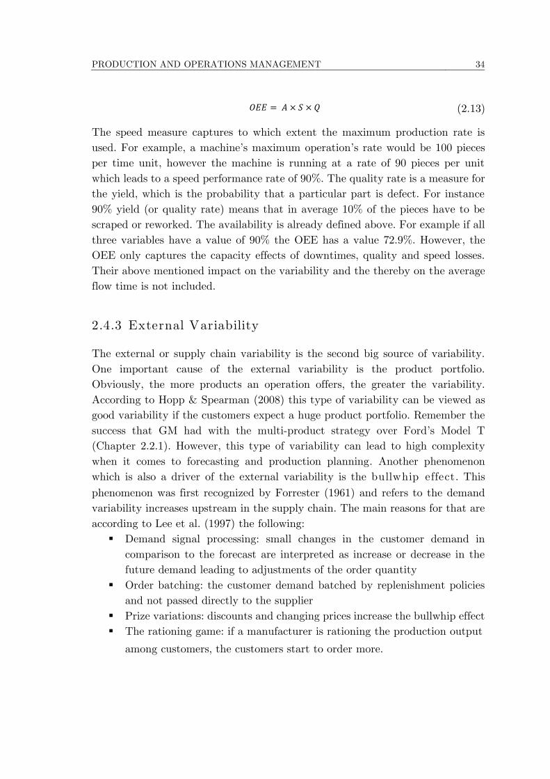
PRODUCTION AND OPERATIONS MANAGEMENT 34
𝑂𝐸𝐸 = 𝐴 × 𝑆 × 𝑄 (2.13)
The speed measure captures to which extent the maximum production rate is
used. For example, a machine’s maximum operation’s rate would be 100 pieces
per time unit, however the machine is running at a rate of 90 pieces per unit
which leads to a speed performance rate of 90%. The quality rate is a measure for
the yield, which is the probability that a particular part is defect. For instance
90% yield (or quality rate) means that in average 10% of the pieces have to be
scraped or reworked. The availability is already defined above. For example if all
three variables have a value of 90% the OEE has a value 72.9%. However, the
OEE only captures the capacity effects of downtimes, quality and speed losses.
Their above mentioned impact on the variability and the thereby on the average
flow time is not included.
2.4.3 External Variability
The external or supply chain variability is the second big source of variability.
One important cause of the external variability is the product portfolio.
Obviously, the more products an operation offers, the greater the variability.
According to Hopp & Spearman (2008) this type of variability can be viewed as
good variability if the customers expect a huge product portfolio. Remember the
success that GM had with the multi-product strategy over Ford’s Model T
(Chapter 2.2.1). However, this type of variability can lead to high complexity
when it comes to forecasting and production planning. Another phenomenon
which is also a driver of the external variability is the bullwhip effect. This
phenomenon was first recognized by Forrester (1961) and refers to the demand
variability increases upstream in the supply chain. The main reasons for that are
according to Lee et al. (1997) the following:
Demand signal processing: small changes in the customer demand in
comparison to the forecast are interpreted as increase or decrease in the
future demand leading to adjustments of the order quantity
Order batching: the customer demand batched by replenishment policies
and not passed directly to the supplier
Prize variations: discounts and changing prices increase the bullwhip effect
The rationing game: if a manufacturer is rationing the production output
among customers, the customers start to order more.
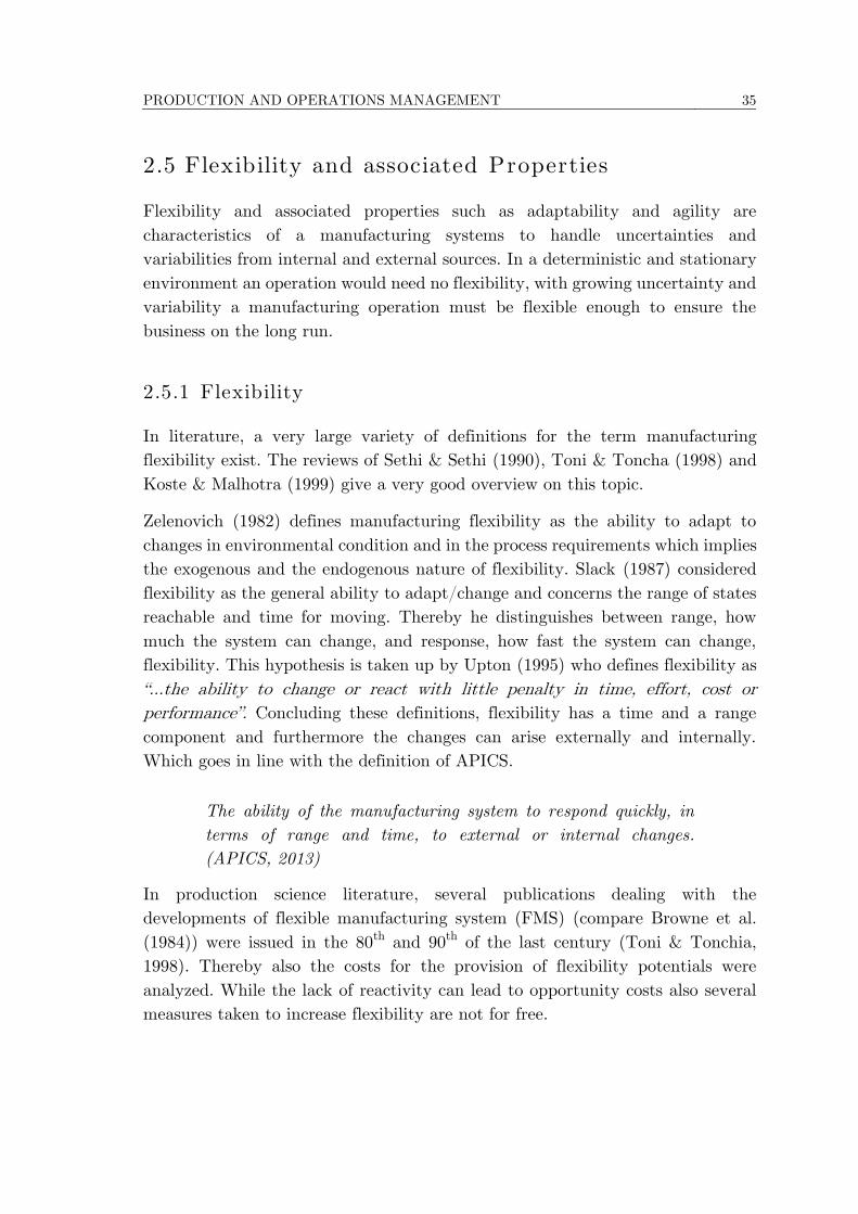
PRODUCTION AND OPERATIONS MANAGEMENT 35
2.5 Flexibility and associated Properties
Flexibility and associated properties such as adaptability and agility are
characteristics of a manufacturing systems to handle uncertainties and
variabilities from internal and external sources. In a deterministic and stationary
environment an operation would need no flexibility, with growing uncertainty and
variability a manufacturing operation must be flexible enough to ensure the
business on the long run.
2.5.1 Flexibility
In literature, a very large variety of definitions for the term manufacturing
flexibility exist. The reviews of Sethi & Sethi (1990), Toni & Toncha (1998) and
Koste & Malhotra (1999) give a very good overview on this topic.
Zelenovich (1982) defines manufacturing flexibility as the ability to adapt to
changes in environmental condition and in the process requirements which implies
the exogenous and the endogenous nature of flexibility. Slack (1987) considered
flexibility as the general ability to adapt/change and concerns the range of states
reachable and time for moving. Thereby he distinguishes between range, how
much the system can change, and response, how fast the system can change,
flexibility. This hypothesis is taken up by Upton (1995) who defines flexibility as
“…the ability to change or react with little penalty in time, effort, cost or
performance”. Concluding these definitions, flexibility has a time and a range
component and furthermore the changes can arise externally and internally.
Which goes in line with the definition of APICS.
The ability of the manufacturing system to respond quickly, in
terms of range and time, to external or internal changes.
(APICS, 2013)
In production science literature, several publications dealing with the
developments of flexible manufacturing system (FMS) (compare Browne et al.
(1984)) were issued in the 80th and 90th of the last century (Toni & Tonchia,
1998). Thereby also the costs for the provision of flexibility potentials were
analyzed. While the lack of reactivity can lead to opportunity costs also several
measures taken to increase flexibility are not for free.
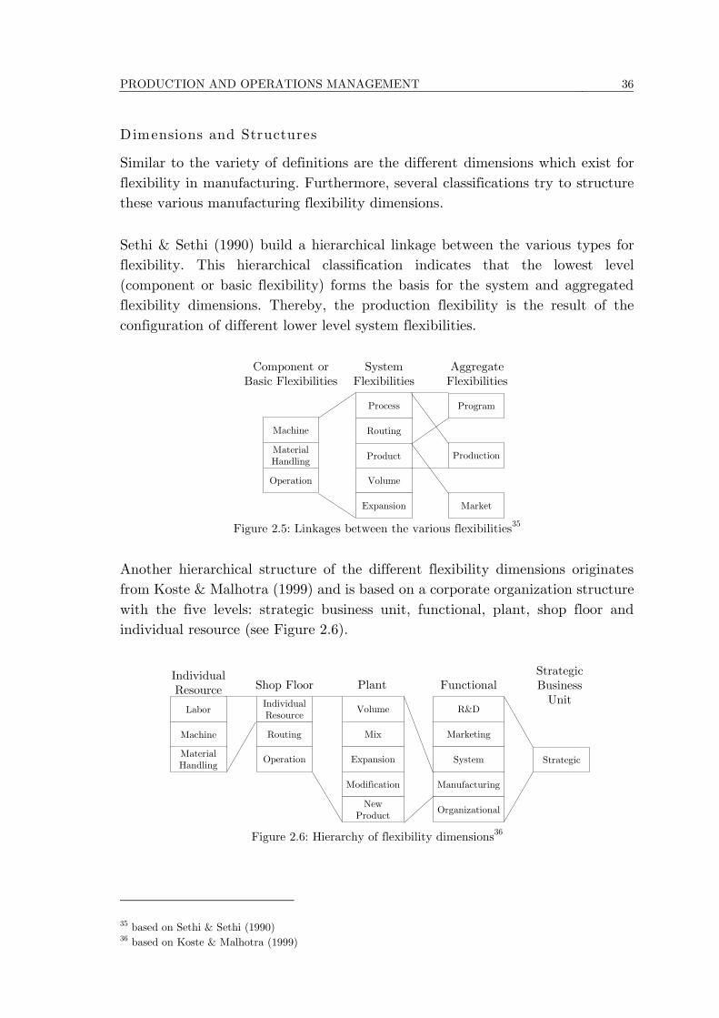
PRODUCTION AND OPERATIONS MANAGEMENT 36
Dimensions and Structures
Similar to the variety of definitions are the different dimensions which exist for
flexibility in manufacturing. Furthermore, several classifications try to structure
these various manufacturing flexibility dimensions.
Sethi & Sethi (1990) build a hierarchical linkage between the various types for
flexibility. This hierarchical classification indicates that the lowest level
(component or basic flexibility) forms the basis for the system and aggregated
flexibility dimensions. Thereby, the production flexibility is the result of the
configuration of different lower level system flexibilities.
Figure 2.5: Linkages between the various flexibilities
35
Another hierarchical structure of the different flexibility dimensions originates
from Koste & Malhotra (1999) and is based on a corporate organization structure
with the five levels: strategic business unit, functional, plant, shop floor and
individual resource (see Figure 2.6).
Figure 2.6: Hierarchy of flexibility dimensions
36
35 based on Sethi & Sethi (1990) 36 based on Koste & Malhotra (1999)
MaterialHandling
Machine
Operation
Process
Routing
Product
Volume
Expansion
Program
Production
Market
Component or Basic Flexibilities
SystemFlexibilities
AggregateFlexibilities
Strategic
R&D
Marketing
System
Manufacturing
Organizational
Volume
Mix
Expansion
Modification
NewProduct
Labor
Machine
Material Handling
StrategicBusiness
UnitFunctionalPlantShop Floor
Individual Resource
Routing
Operation
Individual Resource
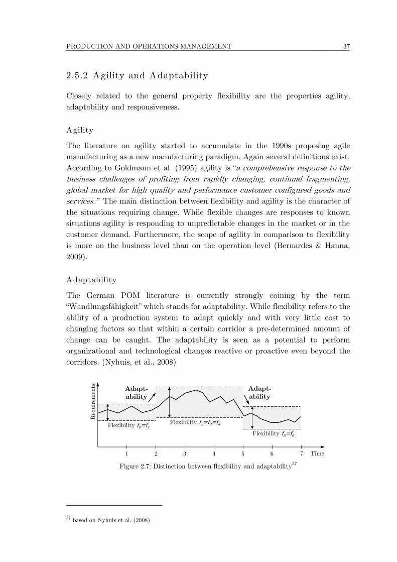
PRODUCTION AND OPERATIONS MANAGEMENT 37
2.5.2 Agility and Adaptability
Closely related to the general property flexibility are the properties agility,
adaptability and responsiveness.
Agility
The literature on agility started to accumulate in the 1990s proposing agile
manufacturing as a new manufacturing paradigm. Again several definitions exist.
According to Goldmann et al. (1995) agility is “a comprehensive response to the
business challenges of profiting from rapidly changing, continual fragmenting,
global market for high quality and performance customer configured goods and
services.” The main distinction between flexibility and agility is the character of
the situations requiring change. While flexible changes are responses to known
situations agility is responding to unpredictable changes in the market or in the
customer demand. Furthermore, the scope of agility in comparison to flexibility
is more on the business level than on the operation level (Bernardes & Hanna,
2009).
Adaptability
The German POM literature is currently strongly coining by the term
“Wandlungsfähigkeit” which stands for adaptability. While flexibility refers to the
ability of a production system to adapt quickly and with very little cost to
changing factors so that within a certain corridor a pre-determined amount of
change can be caught. The adaptability is seen as a potential to perform
organizational and technological changes reactive or proactive even beyond the
corridors. (Nyhuis, et al., 2008)
Figure 2.7: Distinction between flexibility and adaptability
37
37 based on Nyhuis et al. (2008)
Req
uir
emen
ts
1 2 3 4 5 6 Time7
Flexibility f0=f1Flexibility f2=f3=f4
Flexibility f5=f6
Adapt-ability
Adapt-ability
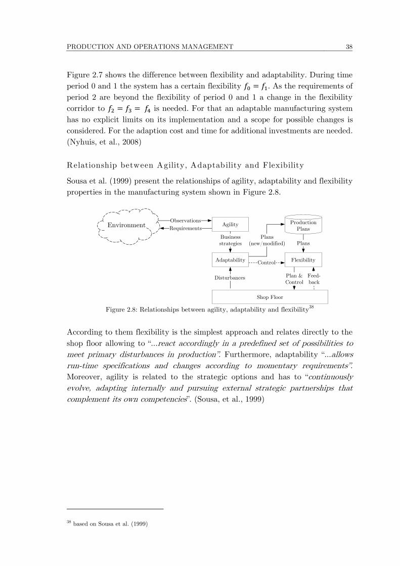
PRODUCTION AND OPERATIONS MANAGEMENT 38
Figure 2.7 shows the difference between flexibility and adaptability. During time
period 0 and 1 the system has a certain flexibility 𝑓0 = 𝑓1. As the requirements of
period 2 are beyond the flexibility of period 0 and 1 a change in the flexibility
corridor to 𝑓2 = 𝑓3 = 𝑓4 is needed. For that an adaptable manufacturing system
has no explicit limits on its implementation and a scope for possible changes is
considered. For the adaption cost and time for additional investments are needed.
(Nyhuis, et al., 2008)
Relationship between Agility, Adaptability and Flexibility
Sousa et al. (1999) present the relationships of agility, adaptability and flexibility
properties in the manufacturing system shown in Figure 2.8.
Figure 2.8: Relationships between agility, adaptability and flexibility
38
According to them flexibility is the simplest approach and relates directly to the
shop floor allowing to “…react accordingly in a predefined set of possibilities to
meet primary disturbances in production”. Furthermore, adaptability “…allows
run-time specifications and changes according to momentary requirements”.
Moreover, agility is related to the strategic options and has to “continuously
evolve, adapting internally and pursuing external strategic partnerships that
complement its own competencies”. (Sousa, et al., 1999)
38 based on Sousa et al. (1999)
EnvironmentObservations
RequirementsAgility
Adaptability Flexibility
Shop Floor
ProductionPlans
Businessstrategies
Disturbances Plan &Control
Feed-back
Plans
Control
Plans(new/modified)
Informatization in
Production
Information is not knowledge. Albert Einstein (1879 – 1955)
Informatization always played a major role in manufacturing. Early after the
invention of the computer concepts based on information technology shaped the
whole manufacturing industry. Nowadays, with the new possibilities of
interconnectivity a further wave of innovation is expected to change the way of
production and also production planning.
This chapter gives an overview on the general definitions as well as the basic
concepts such as computer integrated manufacturing and digital factory.
Moreover, new emerging technologies such as Internet of Things, cyber physical
system and their application in the manufacturing paradigm Industry 4.0 are
explained in this chapter. Also the impacts of the informatization on production
planning and control are shown. Thereby, especially the trends of the increase of
the quantity and quality of data are investigated.
C H A P T E R
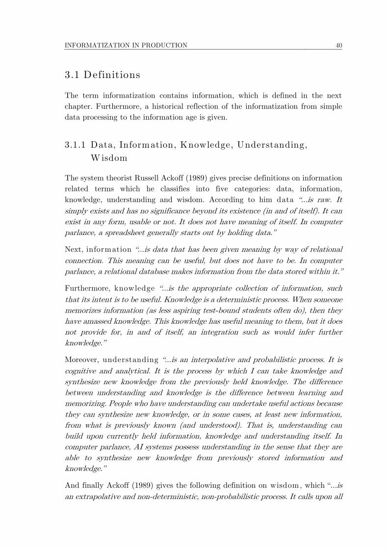
INFORMATIZATION IN PRODUCTION 40
3.1 Definitions
The term informatization contains information, which is defined in the next
chapter. Furthermore, a historical reflection of the informatization from simple
data processing to the information age is given.
3.1.1 Data, Information, Knowledge, Understanding,
W isdom
The system theorist Russell Ackoff (1989) gives precise definitions on information
related terms which he classifies into five categories: data, information,
knowledge, understanding and wisdom. According to him data “…is raw. It
simply exists and has no significance beyond its existence (in and of itself). It can
exist in any form, usable or not. It does not have meaning of itself. In computer
parlance, a spreadsheet generally starts out by holding data.”
Next, information “…is data that has been given meaning by way of relational
connection. This meaning can be useful, but does not have to be. In computer
parlance, a relational database makes information from the data stored within it.”
Furthermore, knowledge “…is the appropriate collection of information, such
that its intent is to be useful. Knowledge is a deterministic process. When someone
memorizes information (as less aspiring test-bound students often do), then they
have amassed knowledge. This knowledge has useful meaning to them, but it does
not provide for, in and of itself, an integration such as would infer further
knowledge.”
Moreover, understanding “…is an interpolative and probabilistic process. It is
cognitive and analytical. It is the process by which I can take knowledge and
synthesize new knowledge from the previously held knowledge. The difference
between understanding and knowledge is the difference between learning and
memorizing. People who have understanding can undertake useful actions because
they can synthesize new knowledge, or in some cases, at least new information,
from what is previously known (and understood). That is, understanding can
build upon currently held information, knowledge and understanding itself. In
computer parlance, AI systems possess understanding in the sense that they are
able to synthesize new knowledge from previously stored information and
knowledge.”
And finally Ackoff (1989) gives the following definition on wisdom , which “…is
an extrapolative and non-deterministic, non-probabilistic process. It calls upon all
INFORMATIZATION IN PRODUCTION 41
the previous levels of consciousness, and specifically upon special types of human
programming (moral, ethical codes, etc.). It beckons to give us understanding
about which there has previously been no understanding, and in doing so, goes
far beyond understanding itself. It is the essence of philosophical probing. Unlike
the previous four levels, it asks questions to which there is no (easily-achievable)
answer, and in some cases, to which there can be no humanly-known answer
period. Wisdom is therefore, the process by which we also discern, or judge,
between right and wrong, good and bad. I personally believe that computers do
not have, and will never have the ability to possess wisdom. Wisdom is a uniquely
human state, or as I see it, wisdom requires one to have a soul, for it resides as
much in the heart as in the mind. And a soul is something machines will never
possess (or perhaps I should reword that to say, a soul is something that, in
general, will never possess a machine).”
Ackoff (1989) indicates also that the first four categories are related to the past,
they deal with “…what has been or what is known”. Only the fifth category,
wisdom deals with “…the future because it incorporates vision and design. With
wisdom people can create the future rather than just grasp the present and past.”
Bellinger et al. (2004) condense the definitions of Ackoff in the following way.
While data are pure symbols, information provides answers to “who”, “what”,
“where”, and “when” questions. Knowledge is the application of data and
information and gives answers on “how” questions. Understanding is the
appreciation of “why” and wisdom is the evaluated understanding. Furthermore,
Bellinger et al. (2004) provide a diagram in which the transition from data, to
information, to knowledge and finally to wisdom is described. In this relationship
understanding is not a separate level, it is instead the support of the transition
from each stage to the next (see Figure 3.1).
Figure 3.1: Relationships between data, information, knowledge and wisdom
39
39 based on (Bellinger, et al., 2004)
understandingrelations
understandingpatterns
understandingprinciples
Connec
tednes
s
UnderstandingData
Information
Knowledge
Wisdom
INFORMATIZATION IN PRODUCTION 42
3.1.2 Informatization
The year of birth of computer lies somewhere in the 1930th or 1940th depending
on the time reckoning. In 1936 Alan Turing40 published the groundbreaking paper
On Computable Numbers (Turing, 1936) in which he suggested a definition on
the term computable. Only numbers that can be calculated with a Turing
machine are considered to be computable. A Turing machine consists of a storage
and a processor, which can perform only simple conversions of zeros and ones. In
1938 Konrad Zuse41 finished his work on Z1, a mechanical device, which could
perform the four basic arithmetical operations. Later on, in 1941 he built the Z3
with the similar logic as the Z1 but based on relay technique. Often in the US
the in 1945 finished ENIAC (Electronic Numerical Integrator and Computer) is
considered as the first electronic general-purpose computer. The ENIAC was
Turing-complete, digital, and initially designed to calculate artillery firing tables
for the United States Army’s Ballistic Research Laboratory (Rojas, 1996).
While in these early days computers were simple data processing machines, later
on the idea of processing data to produce information by computers arose. The
terms information technology (IT) and information and communication
technology (ICT) now describe the computer field. While IT is associated with
hardware and software technologies, ICT stresses more the role of
communications (Davenport, 1997). Marc Porat (1977) categories the ages of
human civilization since the middle age into the agricultural age, the industrial
age and the information age. What industrialization was for the industrial age,
nowadays informatization is for the information age. This process of becoming
information dependent is also known as computerization. According to Castells
(1996) there is even the further trend towards a network society driven by this
informatization.
The term informatization has mostly been used within the context of national
development. However, this trend is currently also taking place in the classical
industrial production and the associated support processes. The next chapter
gives an overview on the IT concepts used in production.
40 Alan Mathison Turing (1912 – 1954) was a British pioneering computer scientist, mathematician, logician,
cryptanalyst, and philosopher. He was highly influential in the development of computer science, providing
a formalization of the concepts of algorithm and computation with the Turing machine, which can be
considered a model of a general purpose computer. Turing is widely considered to be the father of
theoretical computer science and artificial intelligence. 41 Konrad Zuse (1910 – 1995) was a German civil engineer, inventor and computer pioneer. His greatest
achievement was the world’s first functional, program-controlled, Turing-complete computer.
INFORMATIZATION IN PRODUCTION 43
3.2 IT in Production
The need to reduce the time to market with growing demand for more customized
products have let to the excessive use of IT in production. Their application
ranges from simple machining applications to complex PPC optimization
applications. The increasing power and decreasing costs of IT solutions have
spurred these implementations. An early example of the introduction of IT into
the manufacturing world was the concept of computer integrated
manufacturing. This concept favored the enhancement of performance,
efficiency, operational flexibility, product quality, response behavior to market,
differentiations, and time to market. However, the full advantages of IT were
poorly understood at that time and the benefits of computer integrated
manufacturing could not be fully exploited. Later on, the advances in
microprocessor technology, the internet era, standardized software interfaces, the
use of mature techniques for software design and development paved the way for
the excessive use of IT in manufacturing. New concepts such as the digital
factory/manufacturing emerged and there is even the vision of total
interconnected and collaborating factory networks using internet of things and
cyber-physical systems.
3.2.1 Computer Integrated Manufacturing
The initial concept was first recognized by Harrington (1973) who introduced the
name computer integrated manufacturing (CIM) in his book of that title. After
some years, people began to realize the potential benefits of this concept and
several publications on CIM followed.
Definitions
Several definitions of CIM emphasizing various aspects of it as a philosophy, an
organizational structure or the integration of several computer systems exist. The
APICS define CIM as the following:
The integration of the total manufacturing organization through
the use of computer systems and managerial philosophies that
improve the organization’s effectiveness; the application of a
computer to bridge various computerized systems and connect
them into a coherent, integrated whole. For example, budgets,
CAD/CAM, process controls, group technology systems, MRP
II, and financial reporting systems are linked and interfaced.
(APICS, 2013)
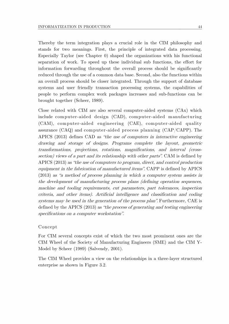
INFORMATIZATION IN PRODUCTION 44
Thereby the term integration plays a crucial role in the CIM philosophy and
stands for two meanings. First, the principle of integrated data processing.
Especially Taylor (see Chapter 0) shaped the organizations with his functional
separation of work. To speed up these individual sub functions, the effort for
information forwarding throughout the overall process should be significantly
reduced through the use of a common data base. Second, also the functions within
an overall process should be closer integrated. Through the support of database
systems and user friendly transaction processing systems, the capabilities of
people to perform complex work packages increases and sub-functions can be
brought together (Scheer, 1989).
Close related with CIM are also several computer-aided systems (CAx) which
include computer-aided design (CAD), computer-aided manufacturing
(CAM), computer-aided engineering (CAE), computer-aided quality
assurance (CAQ) and computer-aided process planning (CAP/CAPP). The
APICS (2013) defines CAD as “the use of computers in interactive engineering
drawing and storage of designs. Programs complete the layout, geometric
transformations, projections, rotations, magnifications, and interval (cross-
section) views of a part and its relationship with other parts”. CAM is defined by
APICS (2013) as “the use of computers to program, direct, and control production
equipment in the fabrication of manufactured items”. CAPP is defined by APICS
(2013) as “a method of process planning in which a computer system assists in
the development of manufacturing process plans (defining operation sequences,
machine and tooling requirements, cut parameters, part tolerances, inspection
criteria, and other items). Artificial intelligence and classification and coding
systems may be used in the generation of the process plan”. Furthermore, CAE is
defined by the APICS (2013) as “the process of generating and testing engineering
specifications on a computer workstation”.
Concept
For CIM several concepts exist of which the two most prominent ones are the
CIM Wheel of the Society of Manufacturing Engineers (SME) and the CIM Y-
Model by Scheer (1989) (Salvendy, 2001).
The CIM Wheel provides a view on the relationships in a three-layer structured
enterprise as shown in Figure 3.2.
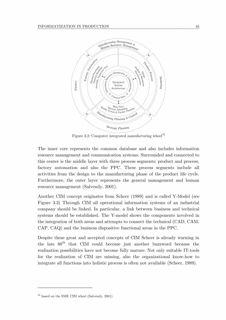
INFORMATIZATION IN PRODUCTION 45
Figure 3.2: Computer integrated manufacturing wheel
42
The inner core represents the common database and also includes information
resource management and communication systems. Surrounded and connected to
this center is the middle layer with three process segments: product and process,
factory automation and also the PPC. These process segments include all
activities from the design to the manufacturing phase of the product life cycle.
Furthermore, the outer layer represents the general management and human
resource management (Salvendy, 2001).
Another CIM concept originates from Scheer (1989) and is called Y-Model (see
Figure 3.3) Through CIM all operational information systems of an industrial
company should be linked. In particular, a link between business and technical
systems should be established. The Y-model shows the components involved in
the integration of both areas and attempts to connect the technical (CAD, CAM,
CAP, CAQ) and the business dispositive functional areas in the PPC.
Despite these great and accepted concepts of CIM Scheer is already warning in
the late 80th that CIM could become just another buzzword because the
realization possibilities have not become fully mature. Not only suitable IT-tools
for the realization of CIM are missing, also the organizational know-how to
integrate all functions into holistic process is often not available (Scheer, 1989).
42 based on the SME CIM wheel (Salvendy, 2001)
Integrated System
Architecture
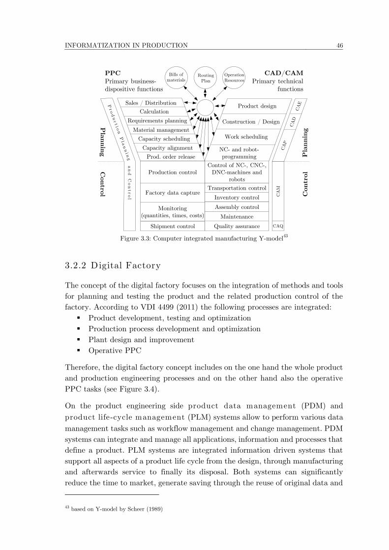
INFORMATIZATION IN PRODUCTION 46
Figure 3.3: Computer integrated manufacturing Y-model
43
3.2.2 Digital Factory
The concept of the digital factory focuses on the integration of methods and tools
for planning and testing the product and the related production control of the
factory. According to VDI 4499 (2011) the following processes are integrated:
Product development, testing and optimization
Production process development and optimization
Plant design and improvement
Operative PPC
Therefore, the digital factory concept includes on the one hand the whole product
and production engineering processes and on the other hand also the operative
PPC tasks (see Figure 3.4).
On the product engineering side product data management (PDM) and
product life-cycle management (PLM) systems allow to perform various data
management tasks such as workflow management and change management. PDM
systems can integrate and manage all applications, information and processes that
define a product. PLM systems are integrated information driven systems that
support all aspects of a product life cycle from the design, through manufacturing
and afterwards service to finally its disposal. Both systems can significantly
reduce the time to market, generate saving through the reuse of original data and
43 based on Y-model by Scheer (1989)
Sales / Distribution
Calculation
Requirements planning
Material management
Capacity scheduling
Capacity alignment
Prod. order release
Production control
Factory data capture
Monitoring (quantities, times, costs)
Shipment control Quality assurance
Inventory control
Assembly control
Transportation control
Maintenance
Control of NC-, CNC-, DNC-machines and
robots
NC- and robot-programming
Work scheduling
Construction / Design
Product design
PPCPrimary business-dispositive functions
CAD/CAMPrimary technical
functions
CAQ
CA
M
an
d C
on
tro
l
Bills of materials
Routing plans
ResourcesRouting Plan
Operation Resources
Pla
nnin
g
Pla
nnin
gC
ontro
l Contr
ol
INFORMATIZATION IN PRODUCTION 47
completely integrate whole engineering workflows (Chryssolouris, et al., 2009).
The common access to a single data base of all product related data furthermore
enables the real time virtual collaboration of globally located teams (Kühn, 2006).
Figure 3.4: Digital factory processes
44
But the concept of the digital factory goes far beyond product engineering. Also
the production engineering such as the design of the plant layout, material flows,
line balancing or offline robotics programming are included (Kühn, 2006). For
that computer simulation has become one of the most used techniques to
design and investigate complex manufacturing systems. Computer simulation
offers a great advantage in the studying and analyzing of the stochastically system
behavior of manufacturing systems. The time and costs for decision making can
thereby be reduced significantly. Digital mock-up (DMU) software packages
allow to visualize the production process, while discrete event simulation
(DES) software helps in the finding of optimal production system settings such
as the location and size of inventory buffers. (Chryssolouris, et al., 2009)
A further recent development is the integration of real-time data from the shop
floor into the digital models. Through the use of wireless technologies on the shop
floor, such as radiofrequency identification (RFID), the accurate and timely
identification of objects, which are moving through the supply chain, is possible
(Chryssolouris, et al., 2009). The basic idea of the interaction of various things
tagged with RFID sensors with their environment is then called Internet of
Things (IoT).
3.2.3 Internet of Things
The Internet of Things (IoT) is the interconnection of uniquely identifiable
devices within the existing Internet infrastructure. According to Atzori et al.
44 based on VDI 4499 (2011)
Research
Development/Design
Facility Planning
Product and Production Process Development
Order Process
Marketing
Purchasing
Job Planning
Production
Sales
Service
INFORMATIZATION IN PRODUCTION 48
(2010) the basic idea of this novel paradigm is “…the pervasive presence around
us of a variety of things or objects – such as RFID tags, sensors, actuators, mobile
phones, etc. which through unique addressing schemes, are able to interact with
each other and cooperate with their neighbors to reach a common goal.”
Unquestionable this visionary concept would have a high impact on several
aspects of everyday life and even more apparent consequences in automation,
manufacturing and logistics. The US National Intelligence Council includes IoT
in the list of the six disruptive civil technologies with potential impact on US
national power. However, as the first definitions of IoT had a mainly things
oriented perspective, RFID is only an enabling forefront technology driving this
vision. Near field communication (NFC) and wireless sensor and actuator
networks (WSAN) are together recognizes with RFID technology as “…the atomic
components that will link the real world with the digital world” (Atzori, et al.,
2010). Together with a middleware software layer several services can be provided
for various applications. In the logistic and production application domain the
real time monitoring of almost every-thing in the supply chain can be enabled by
IoT. This advanced connectivity of objects, devices, systems and services goes far
beyond the classical machine-to-machine (M2M) communications. Smart
industrial management systems would enable an automated control and a real-
time optimization of the production system by using the data provided by a large
number of networked sensors and actuators. These, through networks interacting
elements with physical input and output, are also called cyber physical
systems (Atzori, et al., 2010).
However, IoT also has some open issues and a huge research effort is still needed
to make the IoT concept feasible. One issue is the standardization of RFID and
associated technologies. Another open issue is the addressing of the objects
captures in IoT. Furthermore, there are also serious threats, mainly in respect to
security. IoT is extremely vulnerable to attacks due to the wireless communication
and the most of the time unattached physically easy to attack tags. Because of
the low computation and energy capabilities of IoT components, complex security
schemes are not possible. Finally, also privacy issues have to be clarified, because
through the possibilities of massive data collecting and mining, it would be
impossible for a human individual to personally control the disclosure of their
individual information (Atzori, et al., 2010).
3.2.4 Cyber Physical Systems
According to Lee (2010) there are three main ongoing trends in computing. First,
the data and device proliferation will increase dramatically driven by Moore’s
INFORMATIZATION IN PRODUCTION 49
law45. Sensor networks and portable smart devices are only two examples for that.
The slogan embedded, everywhere from the US National Research Council (2001)
will become true. The second trend is the integration at scale. Because of the fact
that isolation has its costs, the integration from ubiquitous embedded devices to
complex system with global integration will grow in future. The third trend is
due to the biological evolution. The exponential proliferation of embedded devices
is not matched by a corresponding increase in human ability to consume
information. Therefore, there is an ongoing trend of increasing autonomy or
humans out of the loop towards distributed cyber physical information distillation
and control system of embedded devices.
Cyber physical systems (CPS) are defined by Lee (2008) as the following:
Cyber physical systems are integrations of computation with
physical processes. Embedded computers and networks monitor
and control the physical processes, usually with feedback loops
where physical processes affect computations and vice versa.
(Lee, 2008)
The key enabler for CPS is the ability to interact with the physical world and
other embedded controllers through communication. According to Rajkumar et
al. (2010) this integration of computing and communication technologies into
physical systems will transform the physical world around us as the internet
transformed how humans interact with one another. CPS are pushed by several
ongoing technological developments such as low cost and increased capacity
sensors, low-power and high capacity computing devices, wireless communication
technologies and also extensive internet bandwidth. However, the continuous
control of dynamic not entirely predictable physical and engineered system has
still some open issues. Mainly the real-time performance46 of the computerized
control is still an open challenge.
The use of CPS in production systems is also called cyber physical production
system (CPPS). Through such CPPS a quick respond to changing market and
supply chain conditions should be possible. Moreover, real-time information
acquisition of the position and condition of production goods in global supply
chains gets possible. A closer view on the impacts of CPS have especially to PPC
is given in Chapter 3.3.
45 Moore’s law is the observation that, over the history of computing hardware, the number of transistors
in a dense integrated circuit doubles approximately every two years. (Moore, 1998) 46 A real-time system is one which “…controls an environment by receiving data, processing them, and
returning the results sufficiently quickly to affect the environment at that time.” (Martin, 1965)
INFORMATIZATION IN PRODUCTION 50
3.2.5 Industry 4.0
Industry 4.0, the fourth industrial revolution, is a research policy of the German
federal government with the aim to strengthen the German industrial sector (see
detailed aims in Chapter 2.2.3). Within literature various aspects on Industry 4.0
are highlighted and therefore also widely different interpretations exist. However,
the enabling technologies IoT and CPS are nearly mentioned everywhere. In the
white paper of the recommendations for implementing Industry 4.0 the central
statement is that both technologies are coming to the manufacturing environment
to change, or even revolutionize, the way how goods are produced.
In essence, Industry 4.0 will involve the technical integrations of
cyber physical systems into manufacturing and logistics and the
use of the Internet of Things and Services in industrial processes.
This will have implications for value creation, business models,
downstream service and work organization (Plattform Industrie
4.0, 2013).
Huge potentials are expected through this next “revolution” in manufacturing.
Some of them are the following (Plattform Industrie 4.0, 2013):
M eeting individual customer requirements: individual, customer-
specific criteria in the design, configuration, ordering, planning,
manufacture and operation phases and last-minute changes are possible
Flexibility: dynamic configuration through the use of CPS is possible
Optimized decision-taking: through the end-to-end real-time
transparency of all data available
Resource productivity and efficiency: through the continuous
optimized manufacturing processes by CPS
However, some scientists also are of a more critical view regarding the visions of
Industry 4.0. Like CIM, the technology-centered perspective of Industry 4.0 is
ignoring social and organizational aspects in manufacturing. According to
Brödner (2014) a debacle such as with CIM will follow if these deficits are not
solved. There is clear risk of putting all our responsibilities into the hands of
machines. As the automation gets more complex through interdependencies
among algorithms, databases and sensors the potential of failures multiplies. A
small error can cause through system dynamical effects major incidents.
According to Bainbridge (1983) there is even an irony of automation, which means
that the more advanced a control system is, the more crucial may be the
contribution of the human operator, due to the fact that even a highly automated
INFORMATIZATION IN PRODUCTION 51
system needs human beings for supervision, adjustment, maintenance and
improvements.
In that respect also the different perspectives of artificial intelligence (AI)
(Minsky, 1988) and intelligence amplification (IA) (Norman, 1993) have to be
mentioned. While AI stands for smart machines and autonomous agents, IA
emphasis machines (things) that make us smart. This second perspective involves
humans much more in their decision-making and responsibility.
Nevertheless, of these questionable aspects of getting the humans out of the loop,
the further informatization in production will have major influences on the
operative PPC processes which get analyzed in the next chapter.
INFORMATIZATION IN PRODUCTION 52
3.3 IT in Production Planning and Control
In Industry 4.0 the operative PPC is often seen in a real-time machine learning
optimization loop using realistic in-detail models of the production system and
the sensors and actuators of the CPPS. Thereby the vision of continuous
improvements through self-optimization of the controls exist. The real time data
and the tracking of all activities and objects in the real world can be used in PPC.
This new level availability of data will have major impacts on the overall
transparency in the inventory and the shop floor status but will also drive
complexity through the enormous amount of data that can be collected. As one
major trend this quantitative increase of data will lead to decentralized decision
making with the use of agent based computation in manufacturing. Furthermore,
also data quality will experience tremendous improvements through new the
technological possibilities.
3.3.1 Complexity and Decentralized Decision Making
Complex systems, complex relationships and complex problems are coining our
everyday life. Most people also seem to have an intuitive comprehension of
complexity, which somehow has something to do with difficult, incomprehensible,
inscrutable, inexplicable and so on. The research area cybernetics gives in that
respect some more precise answers.
Cybernetics is coming from the Greek term kybernetike, meaning “governance”.
The founder of this research area was Norbert Wiener who describes the term
cybernetics in the title of his book Cybernetics: or Control and Communication
in the Animal and the Machine (Wiener, 1948). The basic finding of cybernetics
is that a system consists in addition to the energy and matter primarily through
the essential basic elements of ordering and organizing information. Cybernetics
distinguishes between simple and complex systems in which simple systems are
no big problems, concerning their regulation and control. Serious problems in the
control only occur if a system is complex. Thereby strictly speaking it is not the
system that must be controlled it is the complexity of the system. The core
question of cybernetics therefore is: How to get the complexity of a system under
control? (Malik, 2002)
The complexity of a system is measureable by using the variety. This term was
introduced by W. Ross Ashby to denote the count of the total number of states
of a system.
Thus, if the order of occurrence is ignored, the collection
INFORMATIZATION IN PRODUCTION 53
c, b, c, a, c, c, a, b, c, b, b, a
which contains twelve elements, contains only three
distinct elements a, b, c. Such a set will be said to have
a variety of three elements. (Ashby, 1956)
While a simple system has only a few possible states a complex system has a
much higher wealth of variants and is therefore much more pretentious to keep
under control. Ashy presented also views on controllers and controlled system
which are nowadays generally used. Among these is also the law of requisite
variety which is today highly prized amount experts of the field of cybernetics.
The law states that a system which controls another is able to compensate more
disturbances in the control process, the greater its variety is.
Only variety can destroy variety. (Ashby, 1956)
This means, in other words, that the only way you can control your destiny is to
be more flexible than your environment. Therefore, any organization must have
as much variety and flexibility as the world around it which is an important
insight. The often used slogan keep it simple has therefore only narrow
authorization. If the environment is complex then the company must be able to
develop sufficient complexity to respond properly (Malik, 2002).
A way to deal with this requested complexity by the law of requisite variety is
decentralized decision making. This basic idea of decentralization and autonomy
is also grounded in the visions of Industry 4.0 with its CPS (Bauernhansl, 2014).
Agent-based computation is here the paradigm which provides the supporting
technology that can handle the new degree of availability of information and has
the ability to process it quickly (Monostori, et al., 2006).
Agent-based Computation
The traditional approach in PPC based on centralized or hierarchical control
structures, presents good characteristic in terms of productivity, especially due to
its optimization capabilities. However, the dynamic and adaptive responses to
change due to increasing volatility of the market and disturbances in
manufacturing disfavor the rigid, top-town hierarchical planning architectures.
Instead systems are needed which can response in real-time to abrupt changes.
Decentered organized, collaborating multi-agent-system fulfill this demanded
property. The theory of these agent-based systems goes back to the early 90s with
the research in distributed artificial intelligence (DAI) (Monostori, et al.,
2006).
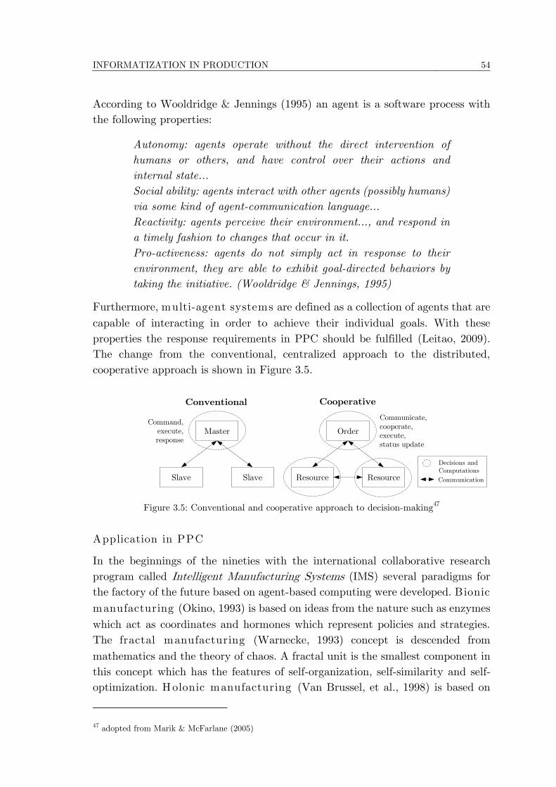
INFORMATIZATION IN PRODUCTION 54
According to Wooldridge & Jennings (1995) an agent is a software process with
the following properties:
Autonomy: agents operate without the direct intervention of
humans or others, and have control over their actions and
internal state…
Social ability: agents interact with other agents (possibly humans)
via some kind of agent-communication language…
Reactivity: agents perceive their environment…, and respond in
a timely fashion to changes that occur in it.
Pro-activeness: agents do not simply act in response to their
environment, they are able to exhibit goal-directed behaviors by
taking the initiative. (Wooldridge & Jennings, 1995)
Furthermore, multi-agent systems are defined as a collection of agents that are
capable of interacting in order to achieve their individual goals. With these
properties the response requirements in PPC should be fulfilled (Leitao, 2009).
The change from the conventional, centralized approach to the distributed,
cooperative approach is shown in Figure 3.5.
Figure 3.5: Conventional and cooperative approach to decision-making
47
Application in PPC
In the beginnings of the nineties with the international collaborative research
program called Intelligent Manufacturing Systems (IMS) several paradigms for
the factory of the future based on agent-based computing were developed. Bionic
manufacturing (Okino, 1993) is based on ideas from the nature such as enzymes
which act as coordinates and hormones which represent policies and strategies.
The fractal manufacturing (Warnecke, 1993) concept is descended from
mathematics and the theory of chaos. A fractal unit is the smallest component in
this concept which has the features of self-organization, self-similarity and self-
optimization. Holonic manufacturing (Van Brussel, et al., 1998) is based on
47 adopted from Marik & McFarlane (2005)
Master Order
Slave Slave Resource Resource Communication
Decisions and Computations
Conventional Cooperative
Communicate,cooperate,execute,status update
Command,execute,response
INFORMATIZATION IN PRODUCTION 55
the concepts of Arthur Koestler who tried to define a hybrid nature of the
structure of living organisms and social groups. Holons are self-containing wholes
to their subordinated parts and can be at the same time a subunit from a larger
system (other holon). Holons have two essential attributes which are autonomous
and cooperative. Good overviews and comparisons on these paradigms can be
found in Tharumarajah, et al. (1998) and Christo & Cardeira (2007).
Nevertheless, all these paradigms suggest that the manufacturing system still need
a hierarchical structure beside the increasing autonomy of the individual entities
in order to resolve inter-entity conflicts and to guarantee the overall goal-
orientation and coherence (Sousa, et al., 1999).
In the visions of Industry 4.0 the CPS and IoT are now seen as the enabling
technology of these agent-based manufacturing paradigms (Bauernhansl, 2014;
Bildstein & Seidelmann, 2014; Hompel & Henke, 2014). Especially the task of real
time manufacturing scheduling involves low-level task assignment and execution
decision with considerable time constraints. Agent-based computation is expected
to provide more reactive and robust solutions in the real-time control of
production processes in comparison to the centralized, rigid top-down structures
of classical PPC (Marik & McFarlane, 2005). Another benefit is the re-
configurability of agent-based solutions, which support the adaptable plug-and-
operate approach. The bottom-up approach, with the separation of the complex
control problem into several smaller simple problems, also leads to simplifications
in debugging and maintenance of the system (Leitao, 2009).
However, there are also some barriers in the application of agent-based solutions
mainly in their costs for implementation in comparison to the classical centralized
solutions. Also no guarantee of operational performance can be made due to the
emergent behaviors of the agents. Furthermore, the scalability of this technology
is limited to the capabilities of the available industrial communication
technologies. Moreover, certain standards and platforms are required for the
interoperability of agent-based systems (Marik & McFarlane, 2005).
3.3.2 Data Quality
According to the quality-guru Juran (1989) data are of high quality if, “…they
are fit for their intended uses in operations, decision making and planning.”
However, many databases contain a surprisingly large number of errors. This poor
data quality has substantial social and economic impacts (Wang & Strong, 1996).
In POM there is a distinction between mainly two different types of data: master
and transactional data. M aster data describe the people, places, and things that
INFORMATIZATION IN PRODUCTION 56
are involved in an organization’s business. Transactional data describe an
internal or external event or transaction that takes place as an organization
conducts its business (McGilvray & Thomas, 2008). Examples for master data
include supplier, customer and material related data as well as bill of materials,
work plans, operations calendars, resources, and so on. Examples for transactional
data include sales orders, purchasing orders, inventories, invoices and so on. Both
types of data require high data quality to ensure the efficient execution of business
processes.
Especially, the broad advent of computer science in the 90’s lead to the research
in data quality, often also called information quality, due to problems in the
definition, measurement and improvement of the quality of data in databases
(Batini & Scannapieca, 2006). At that time the information systems success was
also examined by DeLone & McLean (1992) coming to the finding that the system
quality as well as the information quality form the backbone of the overall success.
In the definition of data quality, the concept of the fitness for use of the data by
data consumers is often used. Wang & Strong (1996) classify the dimensions of
data quality in four categories: intrinsic, contextual, representational and
accessibility data quality. The intrinsic data quality also includes, beside the
traditional viewed accuracy and objectivity, believability and reputation. The
contextual data quality highlights the requirements that data quality must be
considered within the context of the task at hand. One approach for that is to
parametrized the contextual dimensions for each task needed by the data
consumer. The representational data quality emphases aspects related to the
format and meaning of data. Finally, the accessibility has also to be taken into
account (Wang & Strong, 1996). According to Wang & Strong (1996) high quality
data should be “…intrinsically good, contextually appropriate for the task, clearly
represented and accessible to the data customer”. Other sources (Eppler, 2006;
Scheuch, et al., 2012) use similar classifications and overall the timeliness and
accuracy of data can be found in several descriptions.
However, data quality in industrial manufacturing gives a diversified view, which
is far away from high quality data. Apel et al. (2010) give several reasons for the
often poor data quality:
Data capturing: e.g. typing error, shortage of time, misunderstanding,
incorrect data sources
Processes: incorrect disclosure of data
Data corruption: non updated data
Architecture: redundant storage of data, missing interfaces
Data use: inappropriate ambiguous use of data
Definitions: inappropriate definition of the data content or format
INFORMATIZATION IN PRODUCTION 57
According to a German study (Schuh & Stich, 2013), the real-time widespread
crosslinking of production data is so far only partially possible because of the
currently large number of manual system bookings and written documentation.
57% of the small and medium-sized enterprises (SMEs) located in Germany still
use written documentation for the feedback of inventory data from the shop floor.
In large-scale enterprises, 39% still use manually written information flows which
makes real time feedback impossible. The interviewed enterprises also agree to
over 90% on that the integration of IT will make the information flow from the
shop floor to the data consuming departments more transparent and would reduce
manual tasks for data recording, transmission, handling and processing.
As a result of the poor data quality PPC decisions are often based on averages
and estimates (compare Chapter 4.2), which results in inaccurate planning results.
However, the advent of CPS in production with its accurate sensor technique
represents a promising approach to provide the data real-time and in the required
quality needed for a reliable PPC (Hering, et al., 2013). Especially due to the
developments of RFID technology, the data quality of the records of inventory,
the inventory inaccuracy is an often viewed topic in POM science (Kang &
Gershwin, 2004). The inventory inaccuracy occurs when the inventory record,
which is what is available according to the information system, does not match
with the actual physical inventory (DeHoratius & Raman, 2004). To protect
against this issue and its negative impact on the performance of production
planning and control, new methods and policies have to be developed which are
more robust than the traditional one (Chan & Wang, 2014).
Production Planning and
Control
In preparing for battle I have always found that
plans are useless, but planning is indispensable. Dwight Eisenhower (1890 – 1969)
This chapter gives several definitions on the term production planning and control
and the associated tasks. Furthermore, the different concepts of decomposition,
aggregation and disaggregation are explained. Also the typical classification of
production planning and control tasks along the time horizon is shown. Next, the
existing planning approaches get explained and a more detailed description of the
hierarchical planning approach and the used practices is given. In that respect
forecasting, aggregate planning and master production scheduling get explained.
Then the evolution of different production planning and control approaches such
as material requirements planning and just-in-time manufacturing and others is
given. Also a comparison of the two most common planning paradigms push and
pull is given.
C H A P T E R
PRODUCTION PLANNING AND CONTROL 59
4.1 Definitions
The term production planning and control (PPC) consist of two main term which
are: production planning and production control.
4.1.1 Production Planning
The APICS dictionary describes production planning as the following:
A process to develop tactical plans based on setting the overall
level of manufacturing output (production plan) and other
activities to best satisfy the current planned levels of sales (sales
plan or forecasts), while meeting general business objectives of
profitability, productivity, competitive customer lead times, and
so on, as expressed in the overall business plan. The sales and
production capabilities are compared, and a business strategy
that includes a sales plan, a production plan, budgets, pro forma
financial statements, and supporting plans for materials and
workforce requirements, and so on, is developed. One of its
primary purposes is to establish production rates that will achieve
management’s objective of satisfying customer demand by
maintaining, raising, or lowering inventories or backlogs, while
usually attempting to keep the workforce relatively stable. Because
this plan affects many company functions, it is normally prepared
with information from marketing and coordinated with the
functions of manufacturing, sales, engineering, finance,
materials, and so on. (APICS, 2013)
A more general definition for planning is that planning can be understood as the
intellectual anticipation of future events through systematic decision preparation
and making. It includes a decision making process in which solutions of a problem
are searched, evaluated and goal-oriented selected. This is done on the basis of a
monistic or pluralistic objective function with monovalent or polyvalent
expectations. (Kern, 1995)
Also certain tasks are related with the term planning (Koch, 1977):
Definition of the objectives, actions and the needed resources
Coordination of the objectives, sub-plans, actions and resources
Initiate of the plan implementation
Ensure establish reserves for the case of deviation from the plan
PRODUCTION PLANNING AND CONTROL 60
These tasks are executed in the planning process repeatedly until appropriate
operational plans can be initiated. In the operational planning not all task-steps
have to be run through, especially the objectives and resources are determined in
the upstream strategic or tactical planning. The production planning task is
therefore especially at the operational level a well-structured48 problem, which
can be solved by using a model of the system to be planned. (Dangelmaier, 2009)
According to Stachowiak (1973) a model is described by at least three
characteristics:
A model is always a model of something, namely image, representation of
a natural or an artificial original that can be a model itself again.
A model captures generally not all the attributes of the original, but only
those that appear to the model creator relevant.
Models are not clearly assigned to their originals. They perform their
replacement function for certain subjects, within certain time intervals and
restriction to particular mental or physical operations.
4.1.2 Production Control
Besides planning the term PPC also contains production control which is
described by APICS (2013) as “the function of directing or regulating the
movement of goods through the entire manufacturing cycle from the
requisitioning of raw material to the delivery of the finished products”.
According to Dangelmaier (2009) the control in PPC is dealing with the
enforcement of a plan. While production planning itself has no feedback from the
concerned production system, the production control can interact with the
production system.
Especially in the German language there is a more precise separation on the
general term control which would mean directly translated “Steuerung” while
there is also the similar term “Regelung” with a different meaning. According to
DIN (1968) the first term “Steuerung” is a process in a system in which one or
more input variables influence the output values due regularities of the system.
This describes the behavior of a typical input-output system also known as open
loop control. Furthermore, the term “Regelung” is described by DIN (1968) as a
process in which the controlled variable (output) is continuously recorded and
48 A well-structured problem consists of all elements of the problem including a well-defined initial state, a
known goal state, constrained set of local state and constraint parameters. In addition, an algorithm exists
which can determine an optimal decision within the time available. (Greeno, 1978)

PRODUCTION PLANNING AND CONTROL 61
compared with a reference variable (input). Corresponding changes result in an
adjustment through a control variable in the sense of aligning the output to the
reference variable. This behavior is also known as a closed loop control.
As the production control is more than a simple input-output system one should
speak in the German language of a “Produktionsregelung”. However, as the
practice is already used to the term “Produktionsplanung und -Steuerung”, it is
maintained to this inconsistent term. (Kern, 1995)
PRODUCTION PLANNING AND CONTROL 62
4.2 Decomposition, Aggregation and Disaggregation
Decomposition refers to the separation of complex problems into manageable
sub-problems. A prerequisite for such decomposition is that within the overall
problem areas or elements with no or minor relationships in-between can be
identified. A distinction between a horizontal and a vertical decomposition can
be made. In the horizontal decomposition equal sub-problems are identified, while
in the vertical decomposition, there is a hierarchical structure between the sub-
problems. The decomposition of the total production planning task into isolated
sub-problems allows the use of simple solution methods. However, the determined
partial solutions must then be coordinated into an overall solution. (Steven, 1994)
Aggregation is a method of problem simplification through the meaningful
grouping of data and decision variables. This approach results in several
advantages such as the cost and time required for data retrieval can be reduced.
Furthermore, aggregated numbers have a smaller variance than the individual
values, so that prognoses are more reliable. In addition, by the use of a few
aggregate values instead of many individual a better understanding of the basic
relationships and influences can be achieved. Closely related to the concept of
aggregation is the disaggregation, which is the backwards transformation of
aggregated data to a desired level of detail. (Steven, 1994)
In PPC methods these problem simplification techniques are always applied in
certain ways. According to Hopp & Spearman (2008) “the first step in
developing a planning structure is to break down the various decision problems
into manageable sub problems”.
Dangelmaier characterizes planning systems by the following criteria (2009):
Level of Detail refers to the accuracy of planning. A rough planning for
example works with aggregated quantities in scope and time.
Differentiation expresses the depth of the division into subsystems and
their associated sub-plans. Planning tasks can be subdivided by function
and time scope (long, short). The functional subdivision may result in
sales, a production and procurement plan, which build upon each other in
this sequence. The planning horizon and cycle characterizes the time scope
subdivision.
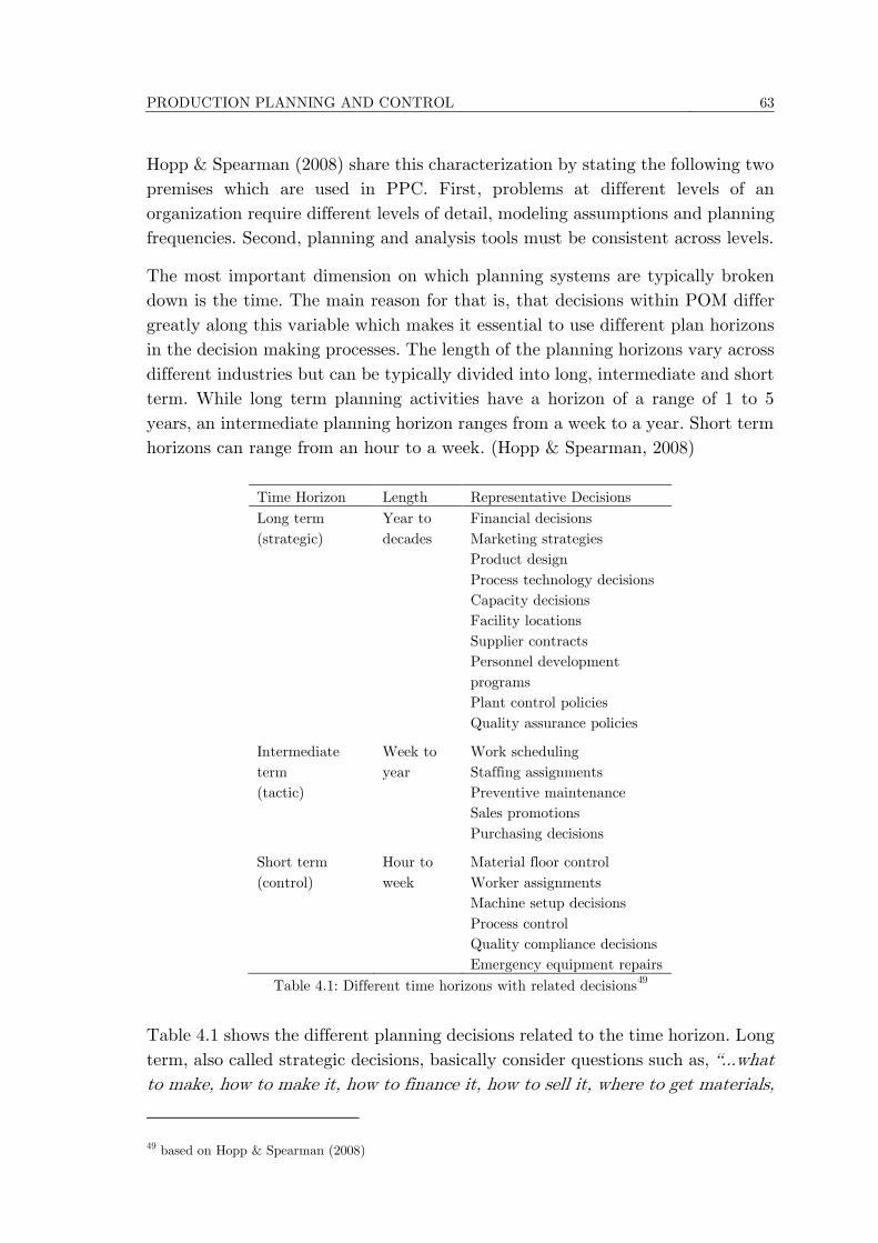
PRODUCTION PLANNING AND CONTROL 63
Hopp & Spearman (2008) share this characterization by stating the following two
premises which are used in PPC. First, problems at different levels of an
organization require different levels of detail, modeling assumptions and planning
frequencies. Second, planning and analysis tools must be consistent across levels.
The most important dimension on which planning systems are typically broken
down is the time. The main reason for that is, that decisions within POM differ
greatly along this variable which makes it essential to use different plan horizons
in the decision making processes. The length of the planning horizons vary across
different industries but can be typically divided into long, intermediate and short
term. While long term planning activities have a horizon of a range of 1 to 5
years, an intermediate planning horizon ranges from a week to a year. Short term
horizons can range from an hour to a week. (Hopp & Spearman, 2008)
Time Horizon Length Representative Decisions
Long term
(strategic)
Year to
decades
Financial decisions
Marketing strategies
Product design
Process technology decisions
Capacity decisions
Facility locations
Supplier contracts
Personnel development
programs
Plant control policies
Quality assurance policies
Intermediate
term
(tactic)
Week to
year
Work scheduling
Staffing assignments
Preventive maintenance
Sales promotions
Purchasing decisions
Short term
(control)
Hour to
week
Material floor control
Worker assignments
Machine setup decisions
Process control
Quality compliance decisions
Emergency equipment repairs
Table 4.1: Different time horizons with related decisions49
Table 4.1 shows the different planning decisions related to the time horizon. Long
term, also called strategic decisions, basically consider questions such as, “…what
to make, how to make it, how to finance it, how to sell it, where to get materials,
49 based on Hopp & Spearman (2008)
PRODUCTION PLANNING AND CONTROL 64
and general principles for the operating system” (Hopp & Spearman, 2008).
Intermediate term, also called tactic decisions, determine “…what to work on, who
will work on it, what actions will be taken to maintain the equipment, what
products will be pushed by sales, and so on” (Hopp & Spearman, 2008). And
finally, short term, also called control decisions, address the movements of
material and workers, adjustments of processes and equipment, and actions
needed to ensure that the system continues to work towards its goal.
These different planning horizons also imply different regeneration frequencies. In
addition to that they also differ in the required level of detail as mentioned above.
In general, it can be said the shorter the horizon the greater the amount of detail
required in the modeling as well as in the data. (Hopp & Spearman, 2008)
Beside time there are also other dimensions on which PPC problems are broken
down such as processes, products and people. As traditionally many operations
are organized according the manufacturing process, it can be reasonable to
separate the planning into the individual process steps. Another form of
aggregation is to combine all products with a similar material routing. Typically,
such combinations are called product families with the definition that within one
family no significant setups are required but there may be setups between families.
(Hopp & Spearman, 2008)
These separations of the decision problems along different dimensions are noting
revolutionary but as it was also mentioned above there is a second premise which
distinguishes a good from a bad system. The difference is not made in how the
problem is broken into sub problems, it is made in how the sub problems are
coordinated with each other (Hopp & Spearman, 2008). This means that long
term planning must be well linked with intermediate planning and a similar link
is needed between intermediate planning and short term planning.
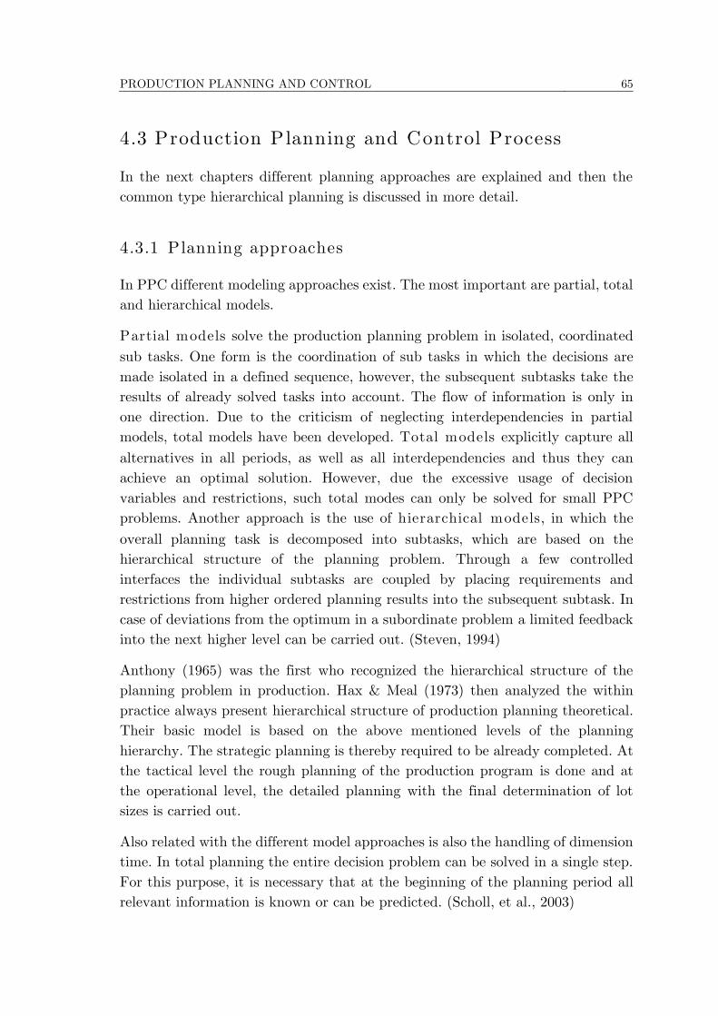
PRODUCTION PLANNING AND CONTROL 65
4.3 Production Planning and Control Process
In the next chapters different planning approaches are explained and then the
common type hierarchical planning is discussed in more detail.
4.3.1 Planning approaches
In PPC different modeling approaches exist. The most important are partial, total
and hierarchical models.
Partial models solve the production planning problem in isolated, coordinated
sub tasks. One form is the coordination of sub tasks in which the decisions are
made isolated in a defined sequence, however, the subsequent subtasks take the
results of already solved tasks into account. The flow of information is only in
one direction. Due to the criticism of neglecting interdependencies in partial
models, total models have been developed. Total models explicitly capture all
alternatives in all periods, as well as all interdependencies and thus they can
achieve an optimal solution. However, due the excessive usage of decision
variables and restrictions, such total modes can only be solved for small PPC
problems. Another approach is the use of hierarchical models, in which the
overall planning task is decomposed into subtasks, which are based on the
hierarchical structure of the planning problem. Through a few controlled
interfaces the individual subtasks are coupled by placing requirements and
restrictions from higher ordered planning results into the subsequent subtask. In
case of deviations from the optimum in a subordinate problem a limited feedback
into the next higher level can be carried out. (Steven, 1994)
Anthony (1965) was the first who recognized the hierarchical structure of the
planning problem in production. Hax & Meal (1973) then analyzed the within
practice always present hierarchical structure of production planning theoretical.
Their basic model is based on the above mentioned levels of the planning
hierarchy. The strategic planning is thereby required to be already completed. At
the tactical level the rough planning of the production program is done and at
the operational level, the detailed planning with the final determination of lot
sizes is carried out.
Also related with the different model approaches is also the handling of dimension
time. In total planning the entire decision problem can be solved in a single step.
For this purpose, it is necessary that at the beginning of the planning period all
relevant information is known or can be predicted. (Scholl, et al., 2003)
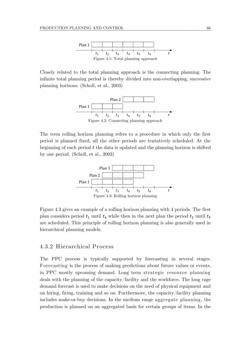
PRODUCTION PLANNING AND CONTROL 66
Figure 4.1: Total planning approach
Closely related to the total planning approach is the connecting planning. The
infinite total planning period is thereby divided into non-overlapping, successive
planning horizons. (Scholl, et al., 2003)
Figure 4.2: Connecting planning approach
The term rolling horizon planning refers to a procedure in which only the first
period is planned fixed, all the other periods are tentatively scheduled. At the
beginning of each period 𝑡 the data is updated and the planning horizon is shifted
by one period. (Scholl, et al., 2003)
Figure 4.3: Rolling horizon planning
Figure 4.3 gives an example of a rolling horizon planning with 4 periods. The first
plan considers period 𝑡1 until 𝑡4 while then in the next plan the period 𝑡2 until 𝑡5
are scheduled. This principle of rolling horizon planning is also generally used in
hierarchical planning models.
4.3.2 Hierarchical Process
The PPC process is typically supported by forecasting in several stages.
Forecasting is the process of making predictions about future values or events,
in PPC mostly upcoming demand. Long term strategic resource planning
deals with the planning of the capacity/facility and the workforce. The long rage
demand forecast is used to make decisions on the need of physical equipment and
on hiring, firing, training and so on. Furthermore, the capacity/facility planning
includes make-or-buy decisions. In the medium range aggregate planning, the
production is planned on an aggregated basis for certain groups of items. In the
Plan 1
Plan 1
Plan 2
Plan 1
Plan 3
Plan 2
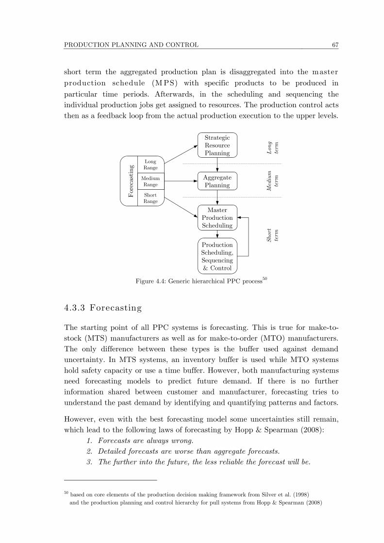
PRODUCTION PLANNING AND CONTROL 67
short term the aggregated production plan is disaggregated into the master
production schedule (M PS) with specific products to be produced in
particular time periods. Afterwards, in the scheduling and sequencing the
individual production jobs get assigned to resources. The production control acts
then as a feedback loop from the actual production execution to the upper levels.
Figure 4.4: Generic hierarchical PPC process
50
4.3.3 Forecasting
The starting point of all PPC systems is forecasting. This is true for make-to-
stock (MTS) manufacturers as well as for make-to-order (MTO) manufacturers.
The only difference between these types is the buffer used against demand
uncertainty. In MTS systems, an inventory buffer is used while MTO systems
hold safety capacity or use a time buffer. However, both manufacturing systems
need forecasting models to predict future demand. If there is no further
information shared between customer and manufacturer, forecasting tries to
understand the past demand by identifying and quantifying patterns and factors.
However, even with the best forecasting model some uncertainties still remain,
which lead to the following laws of forecasting by Hopp & Spearman (2008):
1. Forecasts are always wrong.
2. Detailed forecasts are worse than aggregate forecasts.
3. The further into the future, the less reliable the forecast will be.
50 based on core elements of the production decision making framework from Silver et al. (1998)
and the production planning and control hierarchy for pull systems from Hopp & Spearman (2008)
Strategic ResourcePlanning
MediumRange
For
ecast
ing
LongRange
ShortRange
Master ProductionScheduling
Aggregate Planning
Long
term
Med
ium
term
Short
term
ProductionScheduling,Sequencing& Control
PRODUCTION PLANNING AND CONTROL 68
These laws imply that perfect prediction of the future is not possible.
Furthermore, the concept of variability pooling (aggregation) is a useful approach
in forecasting. And finally the further the forecast goes into the future the greater
the potential of changes is. Overall the main goal in forecasting is to minimize
the difference between the predicted and the real values (forecasting error).
Forecasting is a large science field with many different approaches, nevertheless
a basic distinction can be made between qualitative and quantitative forecasting
(Hopp & Spearman, 2008).
Qualitative Forecasting
Qualitative forecasting methods use the expertise of people rather than
mathematical models. Those approaches are used if no historical data is available,
for example the introduction date of a new product. A structured qualitative
forecasting method is the Delphi method, which was developed to estimate the
number of atomic bombs required to reduce the munitions output by a prescribed
amount. The Delphi method uses repeated individual questioning of experts
through interviews or questionnaires to avoid direct confrontation of the experts
with one another. In this multistep approach information from the experts is
gathered and shared to the other experts in the next round. If the purpose is the
estimation of a numerical quantity the individual estimates will show a tendency
to converge even if the views are initially widely diverged. (Dalkey & Helmer,
1962)
Quantitative Forecasting
Quantitative forecasting methods are based on mathematical models which
predict the future by using historical data. There are two groups of models, causal
models and time series models. Causal models try to predict a future parameter
(e.g. demand of a product) as a function of other parameters (e.g. grows of GDP,
spending in marketing). A common technique used in causal models is regression
analysis. Time series models try to predict future parameters (e.g. demand of
a product) as a function of past values of that parameter (e.g. historical demand).
(Hopp & Spearman, 2008)
According to Silver et al. (1998) a time series is composed of the following five
components: (a) level, (b) trend, (c) seasonal variation, (d) cyclical movements
and (e) irregular random fluctuations. The level captures the scale of a time series.
The trend identifies the rate of grow or decline over the time. Seasonal variation
can arise from natural forces or from human decisions and refer to a periodic
variation of a fairly constant shape. Cyclic variation captures increases and
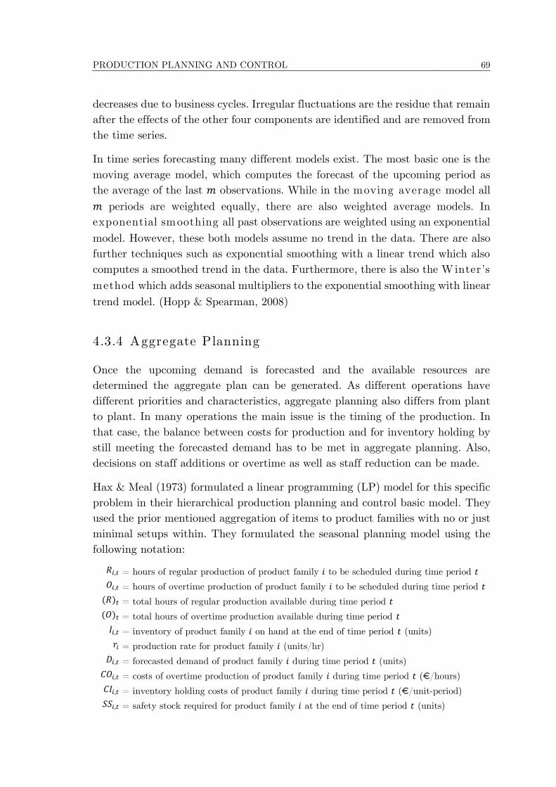
PRODUCTION PLANNING AND CONTROL 69
decreases due to business cycles. Irregular fluctuations are the residue that remain
after the effects of the other four components are identified and are removed from
the time series.
In time series forecasting many different models exist. The most basic one is the
moving average model, which computes the forecast of the upcoming period as
the average of the last 𝑚 observations. While in the moving average model all
𝑚 periods are weighted equally, there are also weighted average models. In
exponential smoothing all past observations are weighted using an exponential
model. However, these both models assume no trend in the data. There are also
further techniques such as exponential smoothing with a linear trend which also
computes a smoothed trend in the data. Furthermore, there is also the Winter’s
method which adds seasonal multipliers to the exponential smoothing with linear
trend model. (Hopp & Spearman, 2008)
4.3.4 Aggregate Planning
Once the upcoming demand is forecasted and the available resources are
determined the aggregate plan can be generated. As different operations have
different priorities and characteristics, aggregate planning also differs from plant
to plant. In many operations the main issue is the timing of the production. In
that case, the balance between costs for production and for inventory holding by
still meeting the forecasted demand has to be met in aggregate planning. Also,
decisions on staff additions or overtime as well as staff reduction can be made.
Hax & Meal (1973) formulated a linear programming (LP) model for this specific
problem in their hierarchical production planning and control basic model. They
used the prior mentioned aggregation of items to product families with no or just
minimal setups within. They formulated the seasonal planning model using the
following notation:
𝑅𝑖,𝑡 = hours of regular production of product family 𝑖 to be scheduled during time period 𝑡
𝑂𝑖,𝑡 = hours of overtime production of product family 𝑖 to be scheduled during time period 𝑡
(𝑅)𝑡 = total hours of regular production available during time period 𝑡
(𝑂)𝑡 = total hours of overtime production available during time period 𝑡
𝐼𝑖,𝑡 = inventory of product family 𝑖 on hand at the end of time period 𝑡 (units)
𝑟𝑖 = production rate for product family 𝑖 (units/hr)
𝐷𝑖,𝑡 = forecasted demand of product family 𝑖 during time period 𝑡 (units)
𝐶𝑂𝑖,𝑡 = costs of overtime production of product family 𝑖 during time period 𝑡 (€/hours)
𝐶𝐼𝑖,𝑡 = inventory holding costs of product family 𝑖 during time period 𝑡 (€/unit-period)
𝑆𝑆𝑖,𝑡 = safety stock required for product family 𝑖 at the end of time period 𝑡 (units)
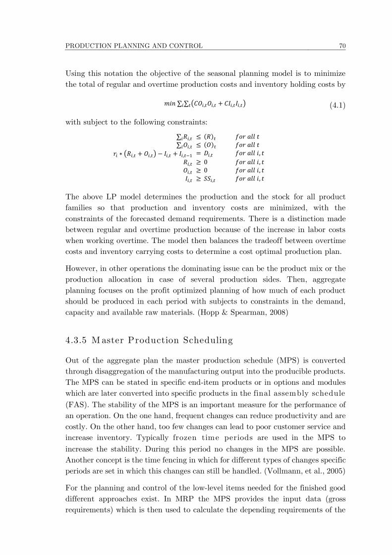
PRODUCTION PLANNING AND CONTROL 70
Using this notation the objective of the seasonal planning model is to minimize
the total of regular and overtime production costs and inventory holding costs by
𝑚𝑖𝑛 ∑𝑖∑𝑡(𝐶𝑂𝑖,𝑡𝑂𝑖,𝑡 + 𝐶𝐼𝑖,𝑡𝐼𝑖,𝑡) (4.1)
with subject to the following constraints:
∑𝑖𝑅𝑖,𝑡 ≤ (𝑅)𝑡 𝑓𝑜𝑟 𝑎𝑙𝑙 𝑡
∑𝑖𝑂𝑖,𝑡 ≤ (𝑂)𝑡 𝑓𝑜𝑟 𝑎𝑙𝑙 𝑡
𝑟𝑖 ∗ (𝑅𝑖,𝑡 + 𝑂𝑖,𝑡) − 𝐼𝑖,𝑡 + 𝐼𝑖,𝑡−1 = 𝐷𝑖,𝑡 𝑓𝑜𝑟 𝑎𝑙𝑙 𝑖, 𝑡
𝑅𝑖,𝑡 ≥ 0 𝑓𝑜𝑟 𝑎𝑙𝑙 𝑖, 𝑡
𝑂𝑖,𝑡 ≥ 0 𝑓𝑜𝑟 𝑎𝑙𝑙 𝑖, 𝑡
𝐼𝑖,𝑡 ≥ 𝑆𝑆𝑖,𝑡 𝑓𝑜𝑟 𝑎𝑙𝑙 𝑖, 𝑡
The above LP model determines the production and the stock for all product
families so that production and inventory costs are minimized, with the
constraints of the forecasted demand requirements. There is a distinction made
between regular and overtime production because of the increase in labor costs
when working overtime. The model then balances the tradeoff between overtime
costs and inventory carrying costs to determine a cost optimal production plan.
However, in other operations the dominating issue can be the product mix or the
production allocation in case of several production sides. Then, aggregate
planning focuses on the profit optimized planning of how much of each product
should be produced in each period with subjects to constraints in the demand,
capacity and available raw materials. (Hopp & Spearman, 2008)
4.3.5 M aster Production Scheduling
Out of the aggregate plan the master production schedule (MPS) is converted
through disaggregation of the manufacturing output into the producible products.
The MPS can be stated in specific end-item products or in options and modules
which are later converted into specific products in the final assembly schedule
(FAS). The stability of the MPS is an important measure for the performance of
an operation. On the one hand, frequent changes can reduce productivity and are
costly. On the other hand, too few changes can lead to poor customer service and
increase inventory. Typically frozen time periods are used in the MPS to
increase the stability. During this period no changes in the MPS are possible.
Another concept is the time fencing in which for different types of changes specific
periods are set in which this changes can still be handled. (Vollmann, et al., 2005)
For the planning and control of the low-level items needed for the finished good
different approaches exist. In MRP the MPS provides the input data (gross
requirements) which is then used to calculate the depending requirements of the
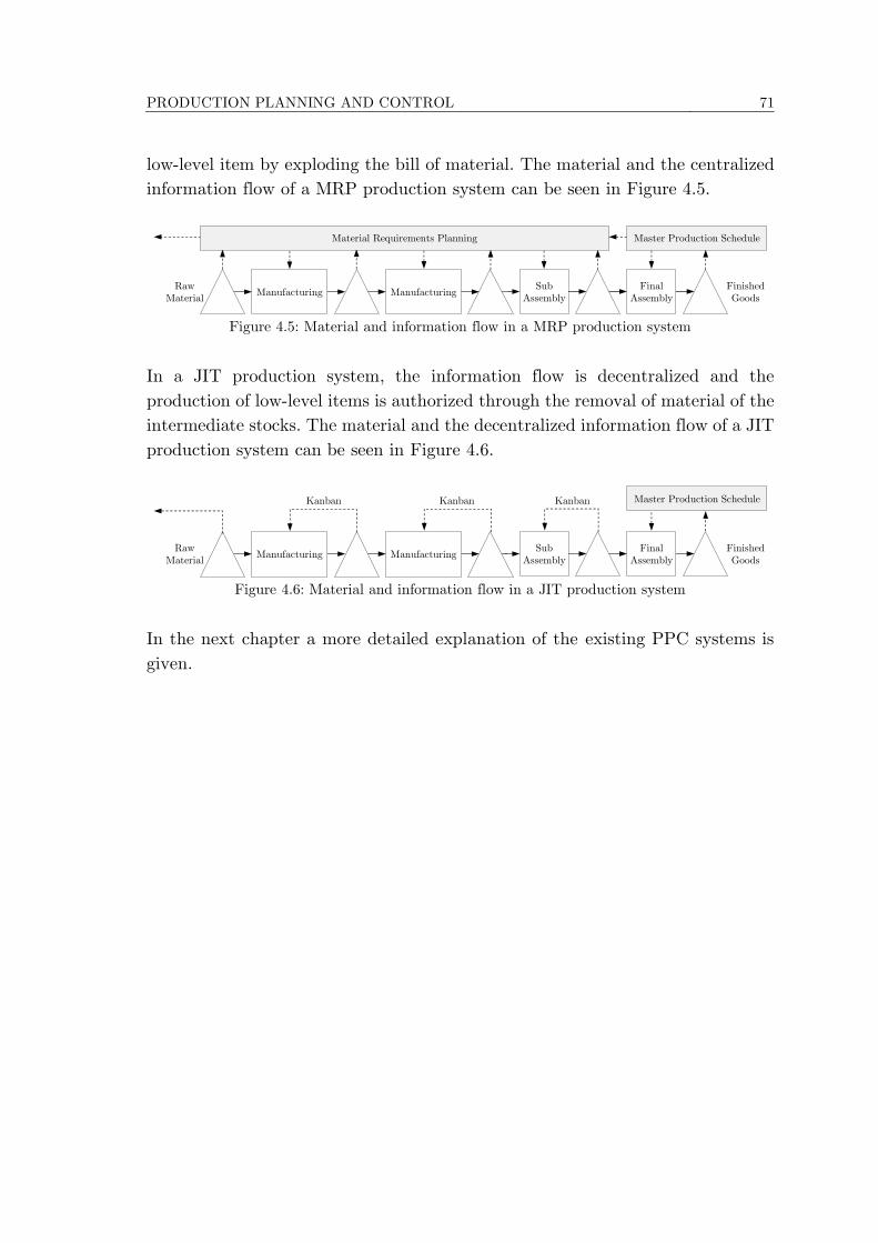
PRODUCTION PLANNING AND CONTROL 71
low-level item by exploding the bill of material. The material and the centralized
information flow of a MRP production system can be seen in Figure 4.5.
Figure 4.5: Material and information flow in a MRP production system
In a JIT production system, the information flow is decentralized and the
production of low-level items is authorized through the removal of material of the
intermediate stocks. The material and the decentralized information flow of a JIT
production system can be seen in Figure 4.6.
Figure 4.6: Material and information flow in a JIT production system
In the next chapter a more detailed explanation of the existing PPC systems is
given.
Finished Goods
Final Assembly
ManufacturingManufacturingSub
AssemblyRaw
Material
Master Production ScheduleMaterial Requirements Planning
Finished Goods
Final Assembly
ManufacturingManufacturingSub
AssemblyRaw
Material
Master Production ScheduleKanbanKanbanKanban
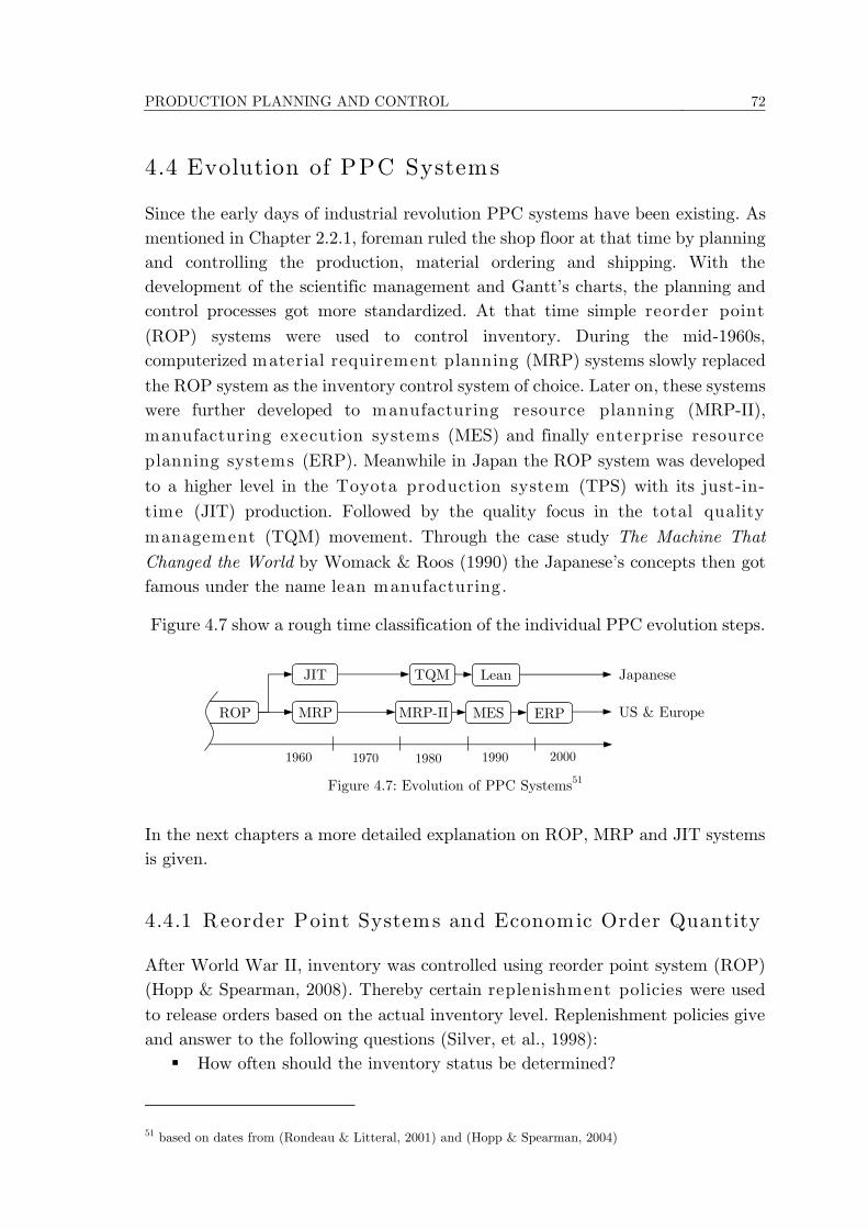
PRODUCTION PLANNING AND CONTROL 72
4.4 Evolution of PPC Systems
Since the early days of industrial revolution PPC systems have been existing. As
mentioned in Chapter 2.2.1, foreman ruled the shop floor at that time by planning
and controlling the production, material ordering and shipping. With the
development of the scientific management and Gantt’s charts, the planning and
control processes got more standardized. At that time simple reorder point
(ROP) systems were used to control inventory. During the mid-1960s,
computerized material requirement planning (MRP) systems slowly replaced
the ROP system as the inventory control system of choice. Later on, these systems
were further developed to manufacturing resource planning (MRP-II),
manufacturing execution systems (MES) and finally enterprise resource
planning systems (ERP). Meanwhile in Japan the ROP system was developed
to a higher level in the Toyota production system (TPS) with its just-in-
time (JIT) production. Followed by the quality focus in the total quality
management (TQM) movement. Through the case study The Machine That
Changed the World by Womack & Roos (1990) the Japanese’s concepts then got
famous under the name lean manufacturing.
Figure 4.7 show a rough time classification of the individual PPC evolution steps.
Figure 4.7: Evolution of PPC Systems
51
In the next chapters a more detailed explanation on ROP, MRP and JIT systems
is given.
4.4.1 Reorder Point Systems and Economic Order Quantity
After World War II, inventory was controlled using reorder point system (ROP)
(Hopp & Spearman, 2008). Thereby certain replenishment policies were used
to release orders based on the actual inventory level. Replenishment policies give
and answer to the following questions (Silver, et al., 1998):
How often should the inventory status be determined?
51 based on dates from (Rondeau & Litteral, 2001) and (Hopp & Spearman, 2004)
1960 1970 1980 1990
ROP MRP MRP-II MES ERP
JIT LeanTQM
US & Europe
Japanese
2000
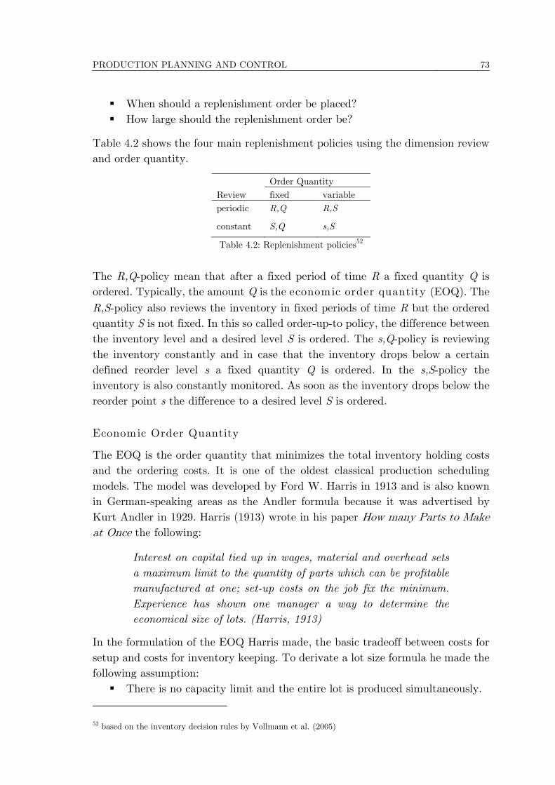
PRODUCTION PLANNING AND CONTROL 73
When should a replenishment order be placed?
How large should the replenishment order be?
Table 4.2 shows the four main replenishment policies using the dimension review
and order quantity.
Order Quantity
Review fixed variable
periodic R,Q R,S
constant S,Q s,S
Table 4.2: Replenishment policies52
The R,Q-policy mean that after a fixed period of time R a fixed quantity Q is
ordered. Typically, the amount Q is the economic order quantity (EOQ). The
R,S-policy also reviews the inventory in fixed periods of time R but the ordered
quantity S is not fixed. In this so called order-up-to policy, the difference between
the inventory level and a desired level S is ordered. The s,Q-policy is reviewing
the inventory constantly and in case that the inventory drops below a certain
defined reorder level s a fixed quantity Q is ordered. In the s,S-policy the
inventory is also constantly monitored. As soon as the inventory drops below the
reorder point s the difference to a desired level S is ordered.
Economic Order Quantity
The EOQ is the order quantity that minimizes the total inventory holding costs
and the ordering costs. It is one of the oldest classical production scheduling
models. The model was developed by Ford W. Harris in 1913 and is also known
in German-speaking areas as the Andler formula because it was advertised by
Kurt Andler in 1929. Harris (1913) wrote in his paper How many Parts to Make
at Once the following:
Interest on capital tied up in wages, material and overhead sets
a maximum limit to the quantity of parts which can be profitable
manufactured at one; set-up costs on the job fix the minimum.
Experience has shown one manager a way to determine the
economical size of lots. (Harris, 1913)
In the formulation of the EOQ Harris made, the basic tradeoff between costs for
setup and costs for inventory keeping. To derivate a lot size formula he made the
following assumption:
There is no capacity limit and the entire lot is produced simultaneously.
52 based on the inventory decision rules by Vollmann et al. (2005)
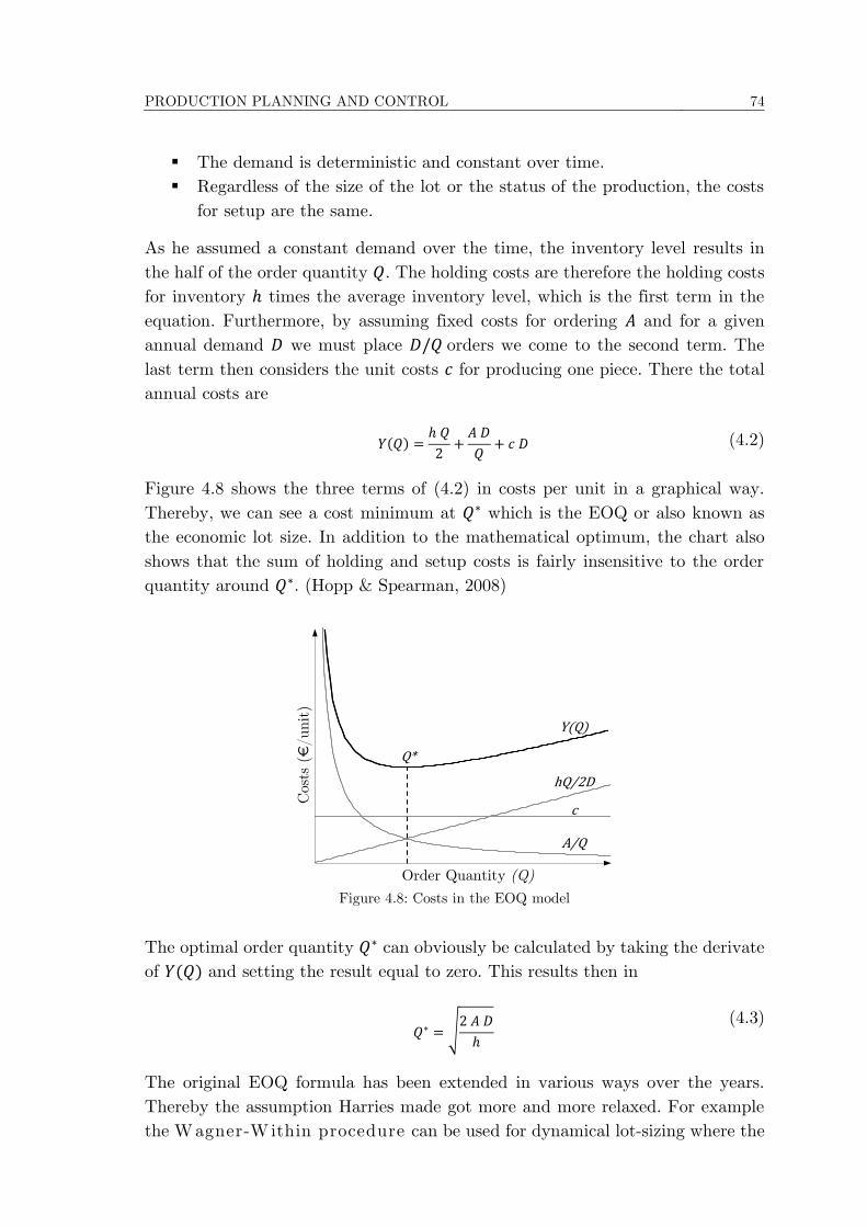
PRODUCTION PLANNING AND CONTROL 74
The demand is deterministic and constant over time.
Regardless of the size of the lot or the status of the production, the costs
for setup are the same.
As he assumed a constant demand over the time, the inventory level results in
the half of the order quantity 𝑄. The holding costs are therefore the holding costs
for inventory ℎ times the average inventory level, which is the first term in the
equation. Furthermore, by assuming fixed costs for ordering 𝐴 and for a given
annual demand 𝐷 we must place 𝐷/𝑄 orders we come to the second term. The
last term then considers the unit costs 𝑐 for producing one piece. There the total
annual costs are
𝑌(𝑄) =ℎ 𝑄
2+
𝐴 𝐷
𝑄+ 𝑐 𝐷 (4.2)
Figure 4.8 shows the three terms of (4.2) in costs per unit in a graphical way.
Thereby, we can see a cost minimum at 𝑄∗ which is the EOQ or also known as
the economic lot size. In addition to the mathematical optimum, the chart also
shows that the sum of holding and setup costs is fairly insensitive to the order
quantity around 𝑄∗. (Hopp & Spearman, 2008)
Figure 4.8: Costs in the EOQ model
The optimal order quantity 𝑄∗ can obviously be calculated by taking the derivate
of 𝑌(𝑄) and setting the result equal to zero. This results then in
𝑄∗ = √2 𝐴 𝐷
ℎ
(4.3)
The original EOQ formula has been extended in various ways over the years.
Thereby the assumption Harries made got more and more relaxed. For example
the Wagner-W ithin procedure can be used for dynamical lot-sizing where the
Cos
ts (
€/u
nit
)
Order Quantity (Q)
Q*
Y(Q)
hQ/2D
A/Q
c
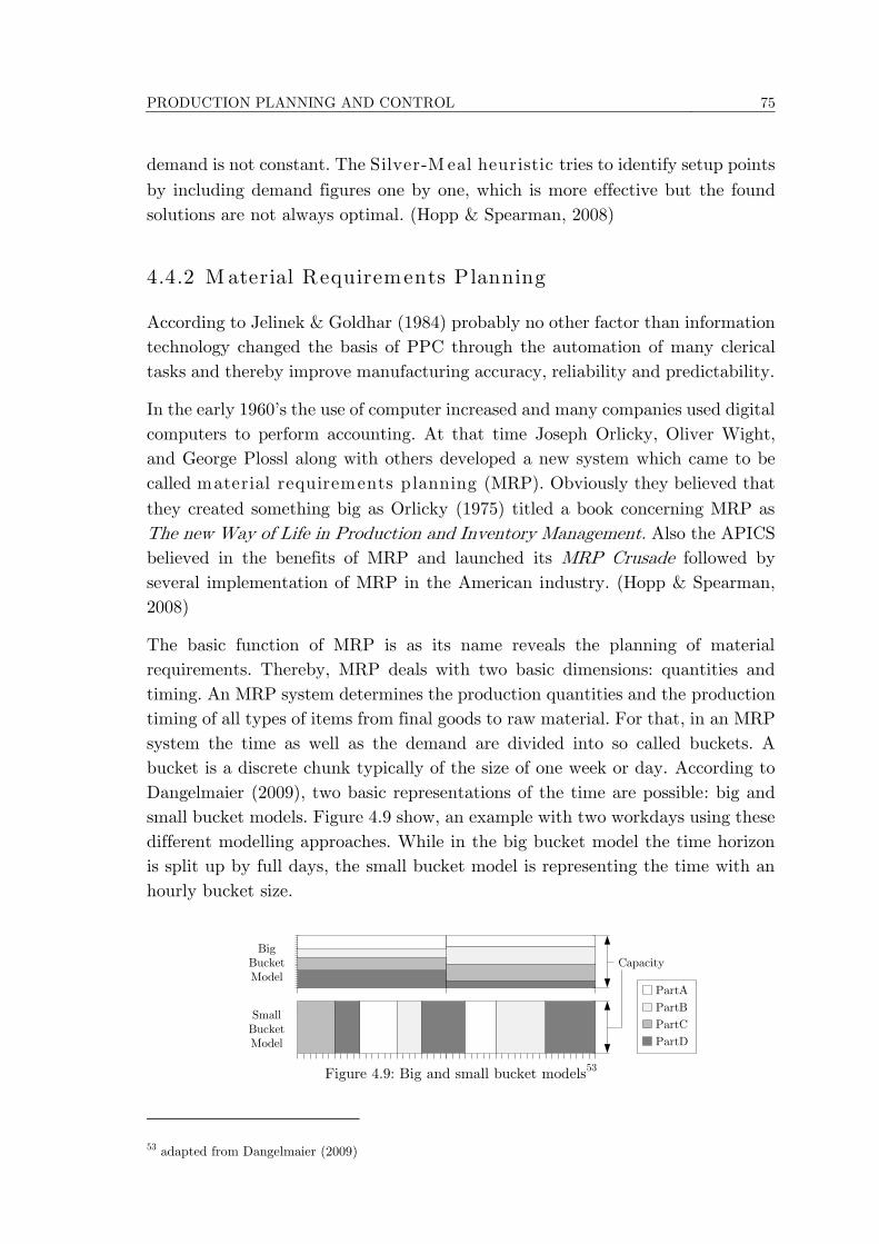
PRODUCTION PLANNING AND CONTROL 75
demand is not constant. The Silver-M eal heuristic tries to identify setup points
by including demand figures one by one, which is more effective but the found
solutions are not always optimal. (Hopp & Spearman, 2008)
4.4.2 M aterial Requirements Planning
According to Jelinek & Goldhar (1984) probably no other factor than information
technology changed the basis of PPC through the automation of many clerical
tasks and thereby improve manufacturing accuracy, reliability and predictability.
In the early 1960’s the use of computer increased and many companies used digital
computers to perform accounting. At that time Joseph Orlicky, Oliver Wight,
and George Plossl along with others developed a new system which came to be
called material requirements planning (MRP). Obviously they believed that
they created something big as Orlicky (1975) titled a book concerning MRP as
The new Way of Life in Production and Inventory Management. Also the APICS
believed in the benefits of MRP and launched its MRP Crusade followed by
several implementation of MRP in the American industry. (Hopp & Spearman,
2008)
The basic function of MRP is as its name reveals the planning of material
requirements. Thereby, MRP deals with two basic dimensions: quantities and
timing. An MRP system determines the production quantities and the production
timing of all types of items from final goods to raw material. For that, in an MRP
system the time as well as the demand are divided into so called buckets. A
bucket is a discrete chunk typically of the size of one week or day. According to
Dangelmaier (2009), two basic representations of the time are possible: big and
small bucket models. Figure 4.9 show, an example with two workdays using these
different modelling approaches. While in the big bucket model the time horizon
is split up by full days, the small bucket model is representing the time with an
hourly bucket size.
Figure 4.9: Big and small bucket models
53
53 adapted from Dangelmaier (2009)
SmallBucketModel
BigBucketModel
PartA
PartB
PartC
PartD
Capacity
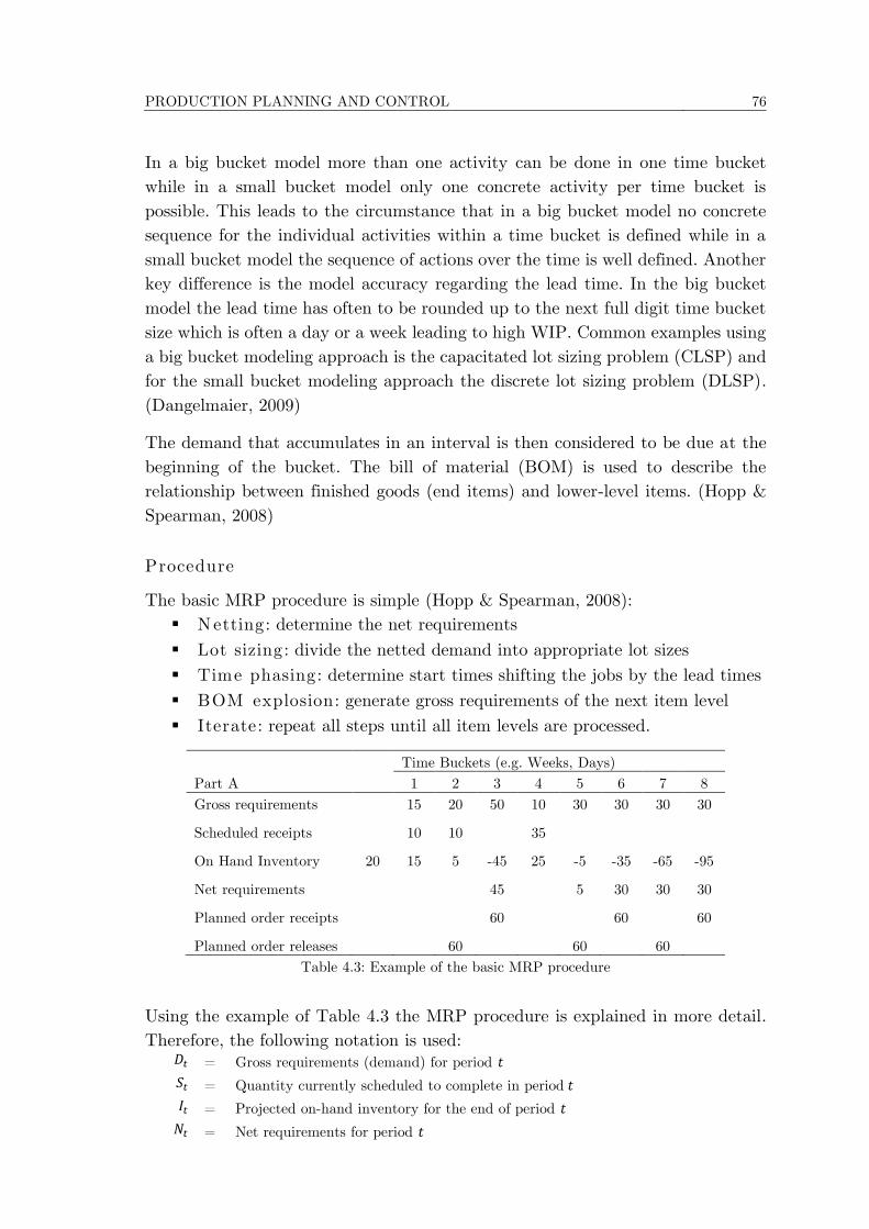
PRODUCTION PLANNING AND CONTROL 76
In a big bucket model more than one activity can be done in one time bucket
while in a small bucket model only one concrete activity per time bucket is
possible. This leads to the circumstance that in a big bucket model no concrete
sequence for the individual activities within a time bucket is defined while in a
small bucket model the sequence of actions over the time is well defined. Another
key difference is the model accuracy regarding the lead time. In the big bucket
model the lead time has often to be rounded up to the next full digit time bucket
size which is often a day or a week leading to high WIP. Common examples using
a big bucket modeling approach is the capacitated lot sizing problem (CLSP) and
for the small bucket modeling approach the discrete lot sizing problem (DLSP).
(Dangelmaier, 2009)
The demand that accumulates in an interval is then considered to be due at the
beginning of the bucket. The bill of material (BOM) is used to describe the
relationship between finished goods (end items) and lower-level items. (Hopp &
Spearman, 2008)
Procedure
The basic MRP procedure is simple (Hopp & Spearman, 2008):
Netting: determine the net requirements
Lot sizing: divide the netted demand into appropriate lot sizes
Time phasing: determine start times shifting the jobs by the lead times
BOM explosion: generate gross requirements of the next item level
Iterate: repeat all steps until all item levels are processed.
Time Buckets (e.g. Weeks, Days)
Part A 1 2 3 4 5 6 7 8
Gross requirements 15 20 50 10 30 30 30 30
Scheduled receipts 10 10 35
On Hand Inventory 20 15 5 -45 25 -5 -35 -65 -95
Net requirements 45 5 30 30 30
Planned order receipts 60 60 60
Planned order releases 60 60 60
Table 4.3: Example of the basic MRP procedure
Using the example of Table 4.3 the MRP procedure is explained in more detail.
Therefore, the following notation is used: 𝐷𝑡 = Gross requirements (demand) for period 𝑡
𝑆𝑡 = Quantity currently scheduled to complete in period 𝑡
𝐼𝑡 = Projected on-hand inventory for the end of period 𝑡
𝑁𝑡 = Net requirements for period 𝑡

PRODUCTION PLANNING AND CONTROL 77
First the projected on hand inventory have to be calculated. For that the current
inventory 𝐼0 must be known. Then the projected-on-hand can be calculated with
𝐼𝑡 = 𝐼𝑡−1 − 𝐷𝑡 + 𝑆𝑡 (4.4)
By subtracting the gross requirements 𝐷𝑡 and adding the already scheduled
receipts from the previous on-hand inventory 𝐼𝑡−1 the next projected on-hand
inventory 𝐼𝑡 can be calculated. Some MRP systems consider in that respect
adjusted scheduled receipts if the current due date of the scheduled receipts is
different to the plan. Next, the net requirements can be computed as
𝑁𝑡 = 𝑚𝑖𝑛{𝑚𝑎𝑥(−𝐼𝑡 , 0), 𝐷𝑡} (4.5)
These net requirements are then used in the lot sizing procedure. There exist
several lot sizing rules used in MRP. The simplest rule is known as lot-for-lot
(LFL), which states that the amount to be produced is equal to the period’s net
requirements. This rule is simple and follows the just in time philosophy, however
it is not considering a tradeoff between setup and inventory holding costs.
Another lot-sizing rule is the use of a fixed order quantity (FOQ), for example
the EOQ. Moreover, a fixed order period (FOP) rule can be used. Thereby, in
predefined periods, the whole accumulated net requirements are planned until the
next fixed order period. Beside this basic rules, many other more advanced rules
exist with the overall goal of a cost optimal schedule. Next, the planned order
receipts get shifted by the planned lead time. Here MRP systems assume that the
time to make a part is fixed, although some systems allow that the planned lead
time is a function of the job size. In the last two steps then, the BOM is used to
transfer the planned order releases as the demand for all depending lower level
items of the just calculated item and rerun the MRP procedure until there are no
lower level items left. (Hopp & Spearman, 2008)
Dealing with Uncertainties
As this above logic of MRP is deterministic, we need something that considers
uncertainty and randomness. There are several sources of uncertainty. First of
all, only in pure make-to-order systems the demand quantity and the timing is
exactly known. In all other production systems, these values are only known by
a certain forecasting reliability. Moreover, machine breakdowns, quality
problems, yield losses and other uncertainties infect the production quantity and
timing. To protect against these issues, safety stock and safety lead times can be
used. Clearly both approaches increase inventory. Silver et al. (1998) provide the
following guideline for copying with uncertainty in MRP. In their opinion, safety
lead time should only be used for raw materials. They suggest to use safety stock:
PRODUCTION PLANNING AND CONTROL 78
for items with direct external usage,
for items produced by a process with significant variable yield,
for items produced at a bottleneck operation
and in semi-finished items which are used for myriad end-items.
Buzacott & Shanthikumar (1994) give a similar answer on the question of using
safety stock or safety lead time. They concluded that safety lead time is only
preferable to safety stock when it is possible to make accurate forecasts demands.
Otherwise safety stock is more robust in dealing with uncertainties.
Weaknesses
However, there are even more challenges in MRP. According to Hopp & Spearman
(2008) the three major ones are (a) long planned lead times, (b) capacity
infeasibility of MRP schedules and (c) system nervousness. Silver et al. (1998)
gives a more detailed overview of significant drawbacks such as the long planned
lead times of MRP:
Lead times: MRP is treading the lead time as an attribute of the part
and not by the status of the shop floor. This means that whether a
department is heavily loaded or underutilized the lead time assumed in
MRP is the same. Therefore, typically lead times are inflated to avoid
schedule problems, which increases obviously the WIP.
Lot sizes: Optimal multi-level, multi-item lot sizing is extremely difficult.
Therefore, MRP relies on heuristics which were already mentioned above.
However, in most of the MRP systems, only the basic lot sizing rules LFL
and EOQ are implemented.
Safety stock: As typically MRP systems do not automatically support
the calculation of safety stocks, these values are set by users which have
typical little knowledge on appropriate safety stock levels.
Incentive for improvement: Another primary weakness of MRP is
directly related with the previous three. Because of the excessive effort to
gather all input data such as safety stock, lead times, lot sizes, and so on,
people tend to not to make any changes on these values. Typically for the
installation of a MRP system is that it is desirable to inflate all these
values to avoid startup problems. However, there is little incentive to dig
through a well working system to change the values to more optimal one
afterwards.
Data consistency: Also a major benefit of MRP is the needed data
accuracy and consistency because an operation must take control of
inventories and schedules. However, in practice consistency of the data
needed for planning is a common problem within MRP systems.
PRODUCTION PLANNING AND CONTROL 79
The basic MRP procedure assumes that all lines have infinite capacity, which
typically creates problems when production is running near to the capacity limit.
Therefore, the basic MRP procedure was later on extended to rough cut
capacity planning (RCCP) and capacity requirements planning (CRP),
which can be both often found in the further development of MRP the
manufacturing resource planning (MRP-II). (Hopp & Spearman, 2008)
System Nervousness
However, one last problem is still there: the so called system nervousness which
refers to the effect that minor changes in the master production schedule can
results in significant changes in the planned order releases (Hopp & Spearman,
2008). The MRP system nervousness was first identified by Steele (1975) who
listed several causes such as MPS changes, unexpected changes in previously made
customer orders, parameter changes (e.g. lead time, safety stock), forecasting
changes, vendor plant fall-down, scrap and spoilage, engineering changes, record
errors and unplanned transactions for this issue.
For example, a demand increase by one piece can lead by an EOQ lot sizing policy
to the production of a further full lot. Clearly, if we use a LFL policy there will
be no larger changes, however this rule typically leads to many setups. In a
guideline to reduce nervousness in MRP system by Vollmann et al. (2005) also
the influence of the selection of an appropriate lot sizing policy is emphasized.
They suggest to use different lot sizing rules for different item levels. One
approach is to use at the top level EOQ, at the intermediate levels either EOQ
or LFL and at the bottom level FOP policies (Vollmann, et al., 2005).
Another way to reduce nervousness is to reduce the changes in the input itself by
freezing the early part of the master production schedule. By using such a frozen
zone at the beginning of the planning horizon, stability can be introduced into
the MRP system and the problems caused by nervousness can be reduced. A
similar concept is to use firm planned orders in MRP to stabilize planning.
(Vollmann, et al., 2005)
Also the updating frequency is a key determinant of the effectiveness of an MRP
system. On the one hand, if we plan too often, the shop floor will be constantly
flooded by changing planned order releases, on the other hand if we plan too
infrequently we could end up with out of date plans. (Hopp & Spearman, 2008)
PRODUCTION PLANNING AND CONTROL 80
4.4.3 Extensions to Material Requirements Planning
Over the years, the basic MRP system got enhanced to avoid some of its main
weaknesses. The following evolution steps were the extension of capacity planning
in manufacturing resource planning (MRP-II), the integration of the shop
floor control in manufacturing execution systems (MES) and finally the
linking of serval operations in an enterprise with the enterprise resource
planning (ERP) systems.
M anufacturing Resource Planning (M RP-II)
As its predecessors, MRP-II also started with a promising book title MRP-II:
Unlocking America’s Productivity Potential (Wight, 1981). MRP-II added
capacity requirements planning (CRP) capabilities to create a closed-loop PPC
system. Now with MRP-II it was possible to integrate material and capacity
requirements and constraints in the calculation of the overall production plan.
CRP calculates the needed capacity through time at each resource by a given
MPS. First a rough cut capacity planning (RCCP) is sometimes performed to
evaluate a tentative MPS. The RCCP is less detailed than the CRP and provides
a quick capacity check of a few critical resources to ensure a feasible MPS. The
second more common type is the CRP in which the MPS is exploded through
MRP. Using the routings of all the individual items the planned order releases
are translated to capacity requirements (for example in machine hours) for each
time bucket and resource. In infinity loading the capacity constrains are ignored
and capacity profiles are calculated. In finite loading the orders are planned
considering the capacity constraints. (Vollmann, et al., 2005)
M anufacturing Execution Systems (M ES)
In the late 1980’s, with the start of the time-based competition, the nature of
manufacturing got more and more dynamic. Processes and products changed
weekly and production schedules even changed on a daily or hourly basis. MRP-
II systems required a high degree of human intervention to create proper plans
and ways to better manage the execution of the shop floor activities were needed.
This was the birth time of manufacturing execution systems (MES) which
generate an interface between MRP-II and the shop floor. While MRP-II is
described as a closed loop PPC system, MRP-II with MES can be seen as a
continuous loop PPC system. Also, information technology was a main driving
force in this integration with the development of automatic identification and
data-collection systems. Bar code readers, radio frequency transponders (RFID)
and other technologies replace people or reduce the chance of making errors in
PRODUCTION PLANNING AND CONTROL 81
the data collection. Also low-cost personal computers, relational databases, local
area network technology and open system standards supported this trend.
(Rondeau & Litteral, 2001)
Enterprise Resource Planning Systems (ERP)
According to Hopp & Spearman the further development was the following:
MRP-III never quite caught on, nor did the indigestibly
acronymed BRP (business requirements planning). Finally, in
spite of its less than appealing acronym, the enterprise resource
planning (ERP) emerged victorious. (Hopp & Spearman, 2008)
This was primarily due to the success a few vendors (e.g. SAP) had in the
integration of several operations such as distribution, accounting, financial,
personal and so on in a whole product. This success of ERP was then mainly
supported by three developments. First of all, the supply chain management
(SCM) trend, which extended the traditional inventory control methods over a
wider scope including distribution, warehousing and multiple production
locations. Second, the business process reengineering (BPR) movement which
led companies to rapidly change their evolved management structures to fit a
software package. And third, the cheap availability of personal computers. (Hopp
& Spearman, 2008)
Advanced Planning Systems (APS)
As it is well known that the strength of ERP systems is not in the area of
planning, advanced planning systems (APS) have been developed to fill this gap.
They are based on the principles of hierarchical planning providing several
solution approaches from mathematical programming and meta-heurists.
(Stadtler, 2005)
As it can be seen in Figure 4.10, the focus of APS is to support the material flow
across all related business functions: procurement, production, distribution and
sales. Furthermore, APS offers several modules for all three levels of aggregation
out of hierarchical planning.
Although this already sounds very promising, there are some drawbacks and
deficiencies of today’s APS. First of all, accurate demand forecasts are a very
important input, hence great emphasis has been put in the development of
forecasting techniques but sophisticated models for demand planning are still rare
in APS. Second, the great integration of all SCM activities in the master planning
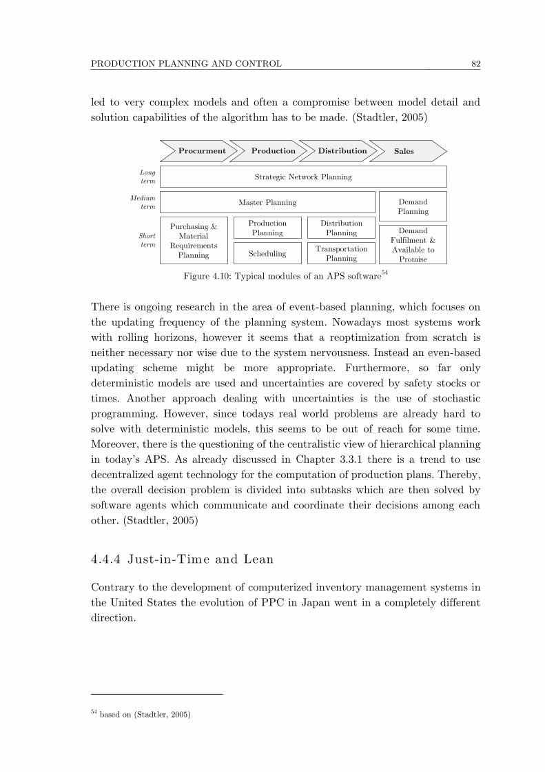
PRODUCTION PLANNING AND CONTROL 82
led to very complex models and often a compromise between model detail and
solution capabilities of the algorithm has to be made. (Stadtler, 2005)
Figure 4.10: Typical modules of an APS software
54
There is ongoing research in the area of event-based planning, which focuses on
the updating frequency of the planning system. Nowadays most systems work
with rolling horizons, however it seems that a reoptimization from scratch is
neither necessary nor wise due to the system nervousness. Instead an even-based
updating scheme might be more appropriate. Furthermore, so far only
deterministic models are used and uncertainties are covered by safety stocks or
times. Another approach dealing with uncertainties is the use of stochastic
programming. However, since todays real world problems are already hard to
solve with deterministic models, this seems to be out of reach for some time.
Moreover, there is the questioning of the centralistic view of hierarchical planning
in today’s APS. As already discussed in Chapter 3.3.1 there is a trend to use
decentralized agent technology for the computation of production plans. Thereby,
the overall decision problem is divided into subtasks which are then solved by
software agents which communicate and coordinate their decisions among each
other. (Stadtler, 2005)
4.4.4 Just-in-Time and Lean
Contrary to the development of computerized inventory management systems in
the United States the evolution of PPC in Japan went in a completely different
direction.
54 based on (Stadtler, 2005)
Longterm
Mediumterm
Shortterm
Procurment Production Distribution Sales
Strategic Network Planning
Master Planning
Purchasing & Material
RequirementsPlanning
ProductionPlanning
Distribution Planning
Demand Planning
SchedulingTransportation
Planning
Demand Fulfilment & Available to
Promise
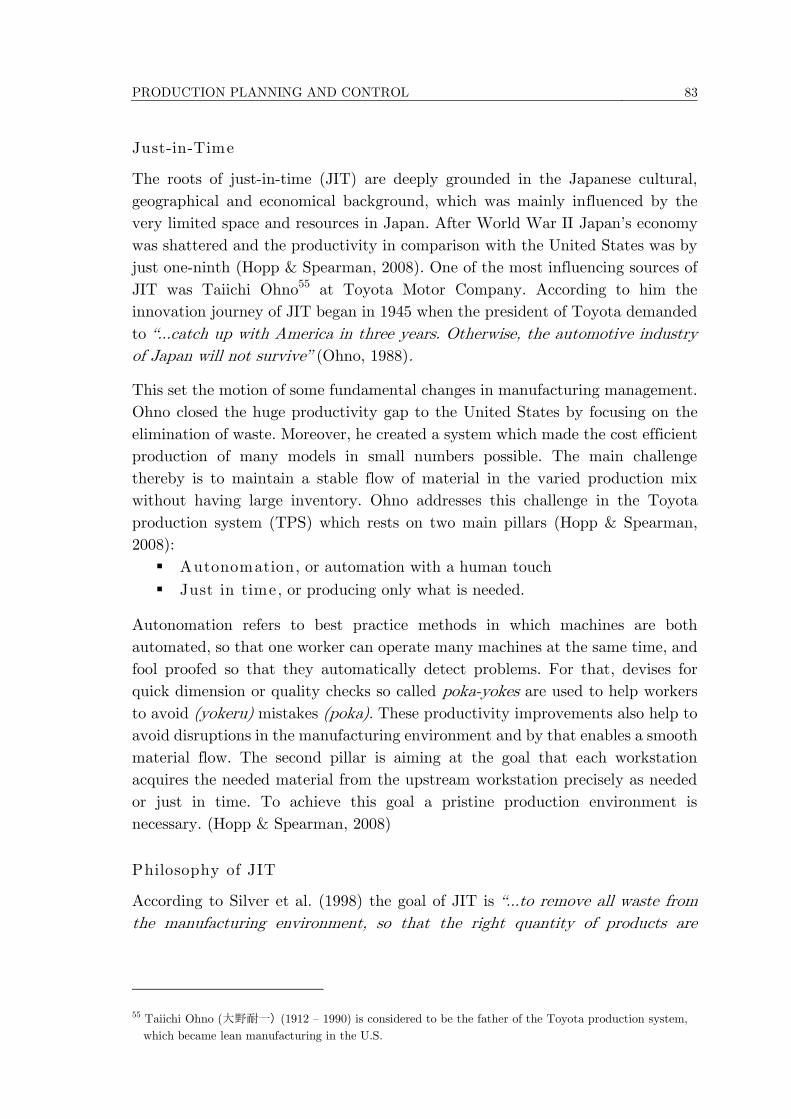
PRODUCTION PLANNING AND CONTROL 83
Just-in-Time
The roots of just-in-time (JIT) are deeply grounded in the Japanese cultural,
geographical and economical background, which was mainly influenced by the
very limited space and resources in Japan. After World War II Japan’s economy
was shattered and the productivity in comparison with the United States was by
just one-ninth (Hopp & Spearman, 2008). One of the most influencing sources of
JIT was Taiichi Ohno55 at Toyota Motor Company. According to him the
innovation journey of JIT began in 1945 when the president of Toyota demanded
to “…catch up with America in three years. Otherwise, the automotive industry
of Japan will not survive” (Ohno, 1988).
This set the motion of some fundamental changes in manufacturing management.
Ohno closed the huge productivity gap to the United States by focusing on the
elimination of waste. Moreover, he created a system which made the cost efficient
production of many models in small numbers possible. The main challenge
thereby is to maintain a stable flow of material in the varied production mix
without having large inventory. Ohno addresses this challenge in the Toyota
production system (TPS) which rests on two main pillars (Hopp & Spearman,
2008):
Autonomation, or automation with a human touch
Just in time, or producing only what is needed.
Autonomation refers to best practice methods in which machines are both
automated, so that one worker can operate many machines at the same time, and
fool proofed so that they automatically detect problems. For that, devises for
quick dimension or quality checks so called poka-yokes are used to help workers
to avoid (yokeru) mistakes (poka). These productivity improvements also help to
avoid disruptions in the manufacturing environment and by that enables a smooth
material flow. The second pillar is aiming at the goal that each workstation
acquires the needed material from the upstream workstation precisely as needed
or just in time. To achieve this goal a pristine production environment is
necessary. (Hopp & Spearman, 2008)
Philosophy of JIT
According to Silver et al. (1998) the goal of JIT is “…to remove all waste from
the manufacturing environment, so that the right quantity of products are
55 Taiichi Ohno (大野耐一) (1912 – 1990) is considered to be the father of the Toyota production system,
which became lean manufacturing in the U.S.
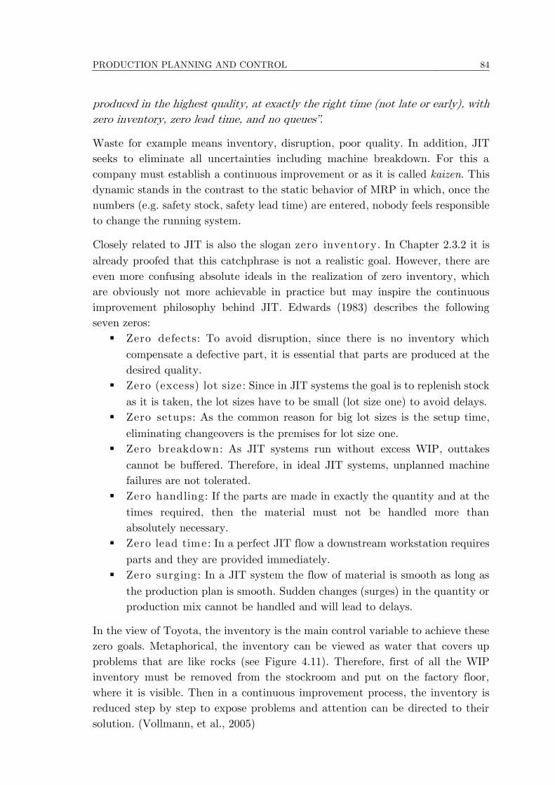
PRODUCTION PLANNING AND CONTROL 84
produced in the highest quality, at exactly the right time (not late or early), with
zero inventory, zero lead time, and no queues”.
Waste for example means inventory, disruption, poor quality. In addition, JIT
seeks to eliminate all uncertainties including machine breakdown. For this a
company must establish a continuous improvement or as it is called kaizen. This
dynamic stands in the contrast to the static behavior of MRP in which, once the
numbers (e.g. safety stock, safety lead time) are entered, nobody feels responsible
to change the running system.
Closely related to JIT is also the slogan zero inventory. In Chapter 2.3.2 it is
already proofed that this catchphrase is not a realistic goal. However, there are
even more confusing absolute ideals in the realization of zero inventory, which
are obviously not more achievable in practice but may inspire the continuous
improvement philosophy behind JIT. Edwards (1983) describes the following
seven zeros:
Zero defects: To avoid disruption, since there is no inventory which
compensate a defective part, it is essential that parts are produced at the
desired quality.
Zero (excess) lot size: Since in JIT systems the goal is to replenish stock
as it is taken, the lot sizes have to be small (lot size one) to avoid delays.
Zero setups: As the common reason for big lot sizes is the setup time,
eliminating changeovers is the premises for lot size one.
Zero breakdown: As JIT systems run without excess WIP, outtakes
cannot be buffered. Therefore, in ideal JIT systems, unplanned machine
failures are not tolerated.
Zero handling: If the parts are made in exactly the quantity and at the
times required, then the material must not be handled more than
absolutely necessary.
Zero lead time: In a perfect JIT flow a downstream workstation requires
parts and they are provided immediately.
Zero surging: In a JIT system the flow of material is smooth as long as
the production plan is smooth. Sudden changes (surges) in the quantity or
production mix cannot be handled and will lead to delays.
In the view of Toyota, the inventory is the main control variable to achieve these
zero goals. Metaphorical, the inventory can be viewed as water that covers up
problems that are like rocks (see Figure 4.11). Therefore, first of all the WIP
inventory must be removed from the stockroom and put on the factory floor,
where it is visible. Then in a continuous improvement process, the inventory is
reduced step by step to expose problems and attention can be directed to their
solution. (Vollmann, et al., 2005)
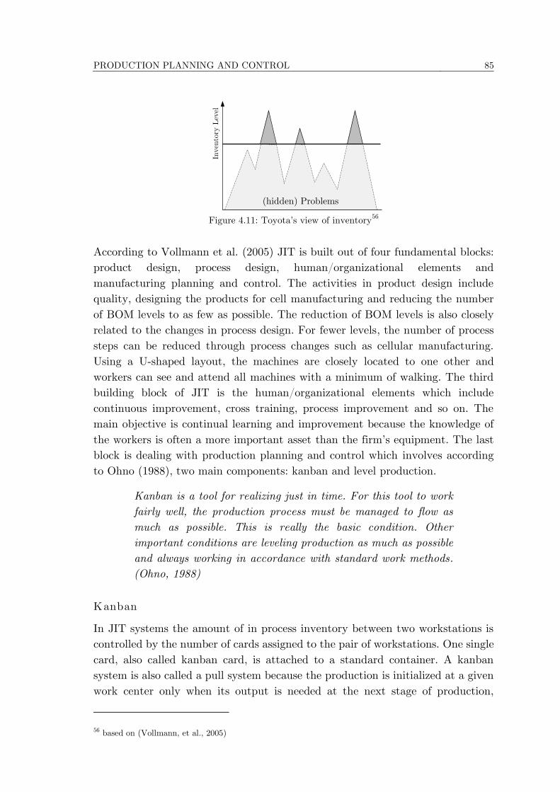
PRODUCTION PLANNING AND CONTROL 85
Figure 4.11: Toyota’s view of inventory
56
According to Vollmann et al. (2005) JIT is built out of four fundamental blocks:
product design, process design, human/organizational elements and
manufacturing planning and control. The activities in product design include
quality, designing the products for cell manufacturing and reducing the number
of BOM levels to as few as possible. The reduction of BOM levels is also closely
related to the changes in process design. For fewer levels, the number of process
steps can be reduced through process changes such as cellular manufacturing.
Using a U-shaped layout, the machines are closely located to one other and
workers can see and attend all machines with a minimum of walking. The third
building block of JIT is the human/organizational elements which include
continuous improvement, cross training, process improvement and so on. The
main objective is continual learning and improvement because the knowledge of
the workers is often a more important asset than the firm’s equipment. The last
block is dealing with production planning and control which involves according
to Ohno (1988), two main components: kanban and level production.
Kanban is a tool for realizing just in time. For this tool to work
fairly well, the production process must be managed to flow as
much as possible. This is really the basic condition. Other
important conditions are leveling production as much as possible
and always working in accordance with standard work methods.
(Ohno, 1988)
Kanban
In JIT systems the amount of in process inventory between two workstations is
controlled by the number of cards assigned to the pair of workstations. One single
card, also called kanban card, is attached to a standard container. A kanban
system is also called a pull system because the production is initialized at a given
work center only when its output is needed at the next stage of production,
56 based on (Vollmann, et al., 2005)
Inven
tory
Lev
el
(hidden) Problems
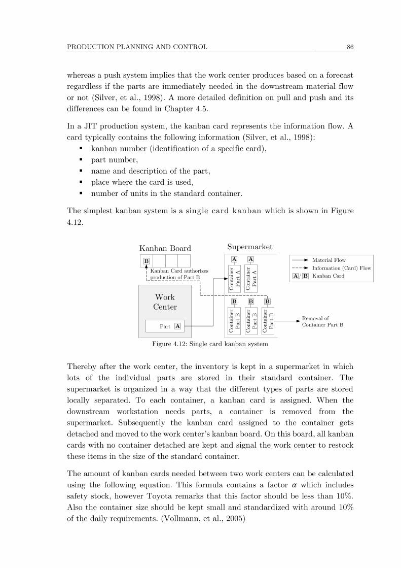
PRODUCTION PLANNING AND CONTROL 86
whereas a push system implies that the work center produces based on a forecast
regardless if the parts are immediately needed in the downstream material flow
or not (Silver, et al., 1998). A more detailed definition on pull and push and its
differences can be found in Chapter 4.5.
In a JIT production system, the kanban card represents the information flow. A
card typically contains the following information (Silver, et al., 1998):
kanban number (identification of a specific card),
part number,
name and description of the part,
place where the card is used,
number of units in the standard container.
The simplest kanban system is a single card kanban which is shown in Figure
4.12.
Figure 4.12: Single card kanban system
Thereby after the work center, the inventory is kept in a supermarket in which
lots of the individual parts are stored in their standard container. The
supermarket is organized in a way that the different types of parts are stored
locally separated. To each container, a kanban card is assigned. When the
downstream workstation needs parts, a container is removed from the
supermarket. Subsequently the kanban card assigned to the container gets
detached and moved to the work center’s kanban board. On this board, all kanban
cards with no container detached are kept and signal the work center to restock
these items in the size of the standard container.
The amount of kanban cards needed between two work centers can be calculated
using the following equation. This formula contains a factor 𝛼 which includes
safety stock, however Toyota remarks that this factor should be less than 10%.
Also the container size should be kept small and standardized with around 10%
of the daily requirements. (Vollmann, et al., 2005)
WorkCenter
Kanban Board
Removal of Container Part B Part A
B
Kanban Card authorizes production of Part B B
Material Flow
Information (Card) Flow
Kanban CardA
Conta
iner
P
art
A
Conta
iner
P
art
A
Conta
iner
P
art
B
Conta
iner
P
art
B
Conta
iner
P
art
B
A A
B B B
Supermarket
PRODUCTION PLANNING AND CONTROL 87
𝐾𝑎𝑛𝑏𝑎𝑛 𝐶𝑎𝑟𝑑𝑠 =𝐷𝑒𝑚𝑎𝑛𝑑 × 𝐿𝑒𝑎𝑑 𝑇𝑖𝑚𝑒 × (1 − 𝛼)
𝐶𝑜𝑛𝑡𝑎𝑖𝑛𝑒𝑟 𝑆𝑖𝑧𝑒 (4.6)
Beside this single card kanban system also different variations exist. In the two
card kanban system, there is a separation between production and move cards.
In this case, there is in addition to the outbound supermarket as it is shown in
the single card kanban system, an inbound supermarket in front of the work
center. The move card authorizes the transfer of standard containers between the
outbound stock point and the inbound stock point of the next work center. The
production card, similar to the single card kanban approves, the production of a
standard container of a specific part to replace the container just taken out of the
outbound supermarket. (Silver, et al., 1998)
Another variation of kanban is the container kanban in which no cards are used.
In such a system, an empty container authorized the production of the specific
parts. Furthermore, signal kanban systems also require no cards. In such a case,
reorder point levels of inventory are directly painted at the shop floor. There also
exists electronically supported kanban (e-kanban) in which the card flow is
replaced by an IT-system. Especially in the assembly lines of automotive industry,
kanban is part of the material supply of a line. Thereby the cards act more as the
above described move cards, because just the consumption driven transportation
of parts from the central warehouse to the assembly line is controlled yet not the
production of the parts. (Klug, 2010)
Heijunka
As mentioned in the zero goals, JIT needs a smooth production plan to work well.
If volumes or product mixes change great in time, it will be difficult for
workstations to replenish the parts just in time (Hopp & Spearman, 2008). This
means, if multiple items are produced in the final assembly operation, it is
required to develop a regular cycle among these items which ensure a smooth
workload. This small cycle times, furthermore, avoid buildup of stock of finished
goods and keep the customer response times short. (Silver, et al., 1998)
This stands quite in contrast to the conventional batch production. If the MPS
requires a monthly production of 10.000 units within the 20 working days in a
mix of 50% part A, 25% part B and 25% part C one would produce the first 10
days part A and then 5 days part B and finally the last 5 days part C. In a JIT
system such a mixed model production looks significantly different. Thereby the
products are sequenced in a smooth way such as
A-B-A-C-A-B-A-C-A-B-A-C-A-B-A-C…
to maintain a constant 50-25-25 mix over the time. (Hopp & Spearman, 2008)
PRODUCTION PLANNING AND CONTROL 88
A measure for the smoothness or flexibility of a production system is the every
part every interval (EPEI) measurement. The EPEI of a production process is
the sum of the processing time for all product variants in the respectively
predetermined batch sizes plus the necessary setup times as well as planned and
unplanned downtime. This value indicates how long it takes for the current
conditions until all variants were produced once. (Erlach, 2010)
To achieve low EPEI values the lot sizes and moreover the setup times have
obviously to be small. For that, JIT offers a further slogan called single minute
exchange die (SMED) which stands for changeover times below 10 minutes
(Hopp & Spearman, 2004). However, such achievements do not happen overnight.
It took Toyota about 25 years to reach this SMED target. According to Ohno
(1988) in 1945, the setup time on a large press was about 2-3 hours, by the 1960s
it could be reduced to 15 minutes and in the 1970 they were down to 3 minutes.
Another concept related to leveling production is the takt time which is the
average unit production time needed to meet customer demand. For the above
example with the 10.000 pieces of demand in 20 work days, this would mean 500
parts per day. In a two shift operation with 480 minutes each shift this then
results in a takt time of 1.92 minutes which is the desired pace of the whole
production system. In reality, it will be unlikely to produce exactly one unit every
1.92 minutes. Here small deviations are no problem, in case of a lines falls back
during one hour it will catch up in the next one. However, the difficulty lies in
the dealing with unexpected disruptions such as machine breakdowns. One way
to avoid a backlog is the use of so called two-shifting. Thereby, two shifts are
scheduled per day which are separated by a down period. This down period can
be used for preventive maintenance or to catch up a backlog. This use of the
capacity buffer is an alternative to the inventory buffer used in most MRP. (Hopp
& Spearman, 2008)
Out of the smooth production flow requirements of JIT, a separate movement
rose which than ultimately become even larger then JIT itself. Hopp & Spearman
(2004) wrote that total quality management (TQM) “…grew into a popular
management doctrine institutionalized in the ISO 9000 Certification process. The
focus on TQM in the 1980’s also spurred Motorola to establish an ambitious
quality goal and to develop a set of statistical techniques for measuring and
achieving it. This approach became known as Six Sigma...”.
LEAN
Outside of Japan, the JIT system became recognized in the 1980s through the
publishing of several books such as Driving the Productivity Machine: Production
PRODUCTION PLANNING AND CONTROL 89
and Control in Japan by Hall (1981), Japanese Manufacturing Techniques: Nine
Hidden Lessons in Simplicity by Schonberger (1982) and finally also Ohno (1988)
published Toyota Production System: Beyond Large Scale Production in English.
At that time companies already become attracted to the simple philosophy and
the inherent techniques. However, depending on how creative and insightful the
managers tying out JIT were it worked sometimes, sometimes not. According to
Hopp & Spearman (2004) Ohno once claimed in an interview that Toyota
considered the system so powerful that they used misleading terms and words to
describe it. However, Toyota was also very open and invited the whole world to
see their factories in the 1980s and 1990s. In 1990, after a 5 year MIT case study,
the book The Machine that Changed the World published by Womack, Jones and
Ross (1990) refreshed the ideas of JIT as lean management. The study compared
several management techniques in the automotive industry in the United States,
Europe and also Japan and concluded that the Japanese methods, especially those
of Toyota, were absolutely superior (Hopp & Spearman, 2004). Under this new
name, the simple techniques of Ohno got again into focus and with “…the help of
an army of consultants, lean became the rage” (Hopp & Spearman, 2008).
Weaknesses
In addition to this incredible success story of JIT and lean weaknesses and
warnings must also be mentioned. However, the probably most dominating notice
is not really a weakness of JIT at all. It is rather the trend that, driven by the
success story of Toyota and big promises of consultants, production manager
implement JIT where it simply does not fit at all. According to Silver (1998) JIT
does not fit in MTO production with high variability which also clearly appears
from the JIT system properties.
JIT is for example not appropriate in job shop where products
are made to order, variability is high, and demand is extremely
nonstationary. Production is not smooth because bottlenecks shift
continually. The high level of variability implies high level of
inventory, but it is difficult to know exactly what inventory to put
into the system when products are all made to order. (Silver, et
al., 1998)
Furthermore, Silver et al. (1998) mention that JIT does not fit to industries such
as process industries where the stages of production are tightly linked. An
interesting comparison for understanding the weaknesses of JIT is done by
Karmarkar (1988). He compares the JIT pull principle with a fast food restaurant
like McDonalds. There, a customer orders a hamburger and the server gets one
from the rack. This then causes the cook to make new one if the number of
PRODUCTION PLANNING AND CONTROL 90
hamburgers in the rack gets too low. This approach works perfectly fine if the
franchise restaurant is downtown with a steady daily stream of customers. But if
it is located next to a football stadium, such a pull system will create an extremely
long queue when the game ends. In such a case, it would be better to push
production according to a forecast.
According to Silver et al. (1998) other weaknesses are that JIT systems are
through the low inventory levels, vulnerable to plant shutdowns, demand surges
and other uncertain events. Furthermore, JIT cannot accommodate frequent
product introduction and phasing outs. Finally, in the amazing success stories the
improvements can not always be directly assigned to JIT programs alone.
4.4.5 Optimized Production Technology
Beside the MRP and the JIT evolution in PPC, there were also many other
smaller trends. One remarkable one is called optimized production technology
(OPT). Along with its principles called theory of constraints (TOC), it got
popular through the book The Goal: A Process of Ongoing Improvement by
Goldratt and Cox (1984). The views on some of the most important operating
performances in OPT are different to MRP and JIT. In OPT, throughput is
viewed as the rate at which a manufacturing firm sells finished goods. Inventory
is the money the firm has invested in purchasing things which it intends to sell.
And finally operating expense is the cost of converting inventory into throughput.
However, the problem is that constraints hinder performance. As the name
already says TOC focuses on constraints such as bottlenecks in production. Like
the continuous improvement in JIT also OPT tries to establish an ongoing
improvement process but the targets are bottleneck resources. Along with other
rules, TOC addresses that “…an hour lost at the bottleneck is an hour lost for the
total system” and “…an hour saved at a nonbottleneck is a mirage” (Silver, et al.,
1998).
PRODUCTION PLANNING AND CONTROL 91
4.5 Push and Pull Principles
The development in POM and PPC is strongly driven by the use of buzzwords.
Push and pull are just two examples of these that stand for different PPC
principles which are commonly used in practice. Unfortunately, their definitions
are not well defined and therefore they are often misunderstood.
The terms pull and lean production have become cornerstones of
modern manufacturing practice. But, although they are widely
used they are less widely understood. (Hopp & Spearman, 2004)
Furthermore, especially in huge science fields such as POM new trends often
create over-reaction.
Like all good revolutions, just in time manufacturing is producing
revolutionaries who don’t know when to stop. (Karmarkar, 1988)
In this chapter the key differences between push and pull principles and their
prominent realizations MRP and kanban get analyzed.
4.5.1 Definitions
First of all, the nature of push and pull systems in general have to be
distinguished. According to Benton & Shin (1998), these terms have been used
decades without clear definition and the use of MRP and JIT with its kanban as
representative of push and pull system has created even more controversy.
Therefore, they provide a good review on this topic showing three different ways
how push and pull can be defined. The most common way to characterize push
and pull system is in term of the order release. In this viewpoint, in a pull system,
an order is triggered by removing an end-item, while in contrast in a push system
the orders are generated by anticipation of future demand. This view is also
shared by Karmarkar (1988). Another way to distinguish between push and pull
is the structure of the information flow. In push systems, the information flow is
centralized and information on customer orders and demand forecasts are used to
release information for all levels of production. In contrast, in a pull system, the
physical flow of material also triggers a local demand information. So in a pure
pull system, the information flow is decentralized. However, using this straight
forward separation the JIT production system also has push elements as the
capacity of the standard containers and the number of kanban cards are
calculated centralized. Finally, the third way to interpret push and pull system is
the WIP level on the shop floor. Hopp & Spearman define a pull system as the
following.
PRODUCTION PLANNING AND CONTROL 92
A pull production system is one that explicitly limits the amount
of work in process that can be in the system. By default, this
implies that a push system is one that has no explicit limit on the
amount of work in process that can be in the system. (Hopp &
Spearman, 2004)
Benton & Shin (1998) conclude, out of this three viewpoints, that if the “…
material flow is initiated by the central planning system without controlling WIP
level, this system is close to the pure push system.” And furthermore “…in a pure
pull system the subsequent process will withdraw (i.e. pull) the parts from the
preceding process using local information and controlling WIP inventory level.”
This leads to the definition that at the shop floor level kanban is a pull system
and MRP works as a push system. However, JIT also using push functions for
example in the long term production planning and the master production
planning. A further view on the definition dilemma is the origin of JIT and MRP.
According to Matsuura et al. (1995) in Japan JIT is understood more as a
philosophy, while MRP is a systematic top down PPC system.
As there rarely exists a pure push or pull production system in practice, many
researchers have realized the possibility of a cohesion between push and pull
principles. In so called hybrid approaches, the idea is that both principles have
their own unique advantages and disadvantages. Through an integration, the
advantages of both systems can be exploited to achieve better performance
(Benton & Shin, 1998). Dickmann (2009) distinguishes in that respect between
vertical hybrid approaches and horizontal hybrid approaches. In a vertical hybrid
approach both principles are integrated redundantly with one other. One example
for that is the CONWIP control developed by Hopp & Spearman which combines
MRP (push) with a WIP cap (pull) using cards in a broadly similar fashion as
kanban does. In a horizontal hybrid approach, the push and pull principles are
used parallel for different product families. For example, for less valuable items
kanban (pull) is used while for expensive highly customized parts MRP (push)
controls the production.
4.5.2 Comparison Studies
Since the attention of the industry on JIT techniques several push/pull
comparison studies have been made. Karmarkar (1988) recognized that the
kanban system can also be seen as a simple s,Q system (compare the
replenishment policies of Chapter 4.4.1). The reorder point s is the number of
kanban cards and the order quantity Q is the size of a standard container.
However, MRP can be viewed as an s,Q system as well. Axsäter & Rosling (1994)
PRODUCTION PLANNING AND CONTROL 93
show that MRP is even more general than an s,Q-policy so that any s,Q system
can be replaced by an MRP system. Silver et al. (1998) concluded out of that,
that MRP dominates both, kanban and s,Q, because it is more general and can
imitate either.
…JIT is not better for certain environment. For example, in
multistage, system where end item demand fluctuates widely, the
kanban system does not work well. Moreover, even when end item
demand is relatively level, fluctuation in component
requirements, can be caused by batching decisions that are made
because of high setup times/costs. So if there are significant setup
times, and parts are therefore batched for production, dependent
demand will fluctuate widely and kanban and s,Q system will not
be appropriate. A related reason is that if there are multiple
items, and high changeover times between items, batching will be
necessary. (Silver, et al., 1998)
Therefore, kanban only applies in high volume lines where setup times are low,
small lot sizes are used, and variability in demand is not amplified back through
the system. But Silver et al. (1998) give additionally an answer to the question
why JIT is then such an improvement on MRP. As already discussed, MRP is
lacking in incentives for improvement. In the decentralized nature of the manual
controlled kanban, improvements are far easier to implement, but that does not
mean that MRP cannot fit into a continuous improvement environment.
One of the earliest and largest conducted analytical comparison studies of MRP
and JIT was performed by Krajewski et al. (1987). In this study, a massive
simulation based analysis of thirty-six factors that influence the performance of a
production system was made. The factors were clustered into:
customer influences, including forecast errors
vendor influences, including vendor quality and lead time variability
buffer mechanisms, including capacity and inventory buffers
product structure, including BOM levels
facility design, including routing pattern and length
process, including scrap, breakdowns and worker flexibility
inventory, including inventory accuracy and lot sizes
as well as some other factors.
Thereby, Krajewski et al. (1987) concluded that changing these factors is more
important than the used scheduling system.
The performance of kanban was quite impressive in our
experiments. However, the natural question arises as to how much
PRODUCTION PLANNING AND CONTROL 94
of this performance is attributable to the kanban system as
opposed to the manufacturing environment in which it was
applies… The reason why kanban appears attractive is not the
system itself. A reorder point system does just as well. The
kanban system merely is a convenient way to implement a small
lot strategy and a way to expose environmental problems.
(Krajewski, et al., 1987)
So it is mainly the flow environment established through the JIT philosophy
which makes the difference. However, there is no point that such an environment
can be established and then run by an MRP system. However, Krajewski et al.
(1987) also mention that as kanban is a paperless system, no excessive
documentation with high administrative costs like in a MRP system is needed.
Also other simulation studies for example Steele & Russell (1990) conclude that
the JIT production environment with its small setup times and lot sizes is the
critical factor for the superior performance of such a production system.
Spearman & Zazanis (1992) found out that it is not the pull principle itself, it is
the limit in the level and variability of WIP inventory which leads to superior
performance. Furthermore, they mention that “push system control throughput
by establishing a master production schedule and measure WIP to detect
problems in meeting a schedule”. In contrast “pull system control WIP and must
measure throughput against required demand”.
Sarker & Firtzsimmons (1989) claim the possibility of a low utilization when the
machines are not balanced perfectly as a potential problem of the pull system.
Plenert (1999) found the same issue by analyzing labor efficiencies in push and
pull system. He claims that JIT was developed in Japan during a time when
resources and capital was limited and the unemployment was high. Therefore, the
clear focus was on material efficiency and not on high utilization of labor or
equipment.
According to Benton & Shin (1998) the “difficulties in comparing MRP and JIT
production systems originate from the fact that MRP was developed as a planning
tool and kanban as a control device. The strength of MRP is in long range
planning, scheduling, material planning and coordination… In contrast, JIT
production systems are effective systems for the shop floor scheduling and to
control. Thus the integration of MRP and kanban would allow firms to improve
manufacturing effectivity and customer service level.” Therefore, in several
hybrid approaches, MRP can be seen as the main planning tool, while kanban
acts as the control mechanism on the shop floor. Benton & Shin (1998) state that
there is no reason why centralized planning information should not be used in a
PRODUCTION PLANNING AND CONTROL 95
JIT production system. Otherwise kanban control mechanism can be used to
execute the production plan in a MRP based manufacturing environment.
As mentioned in the weaknesses of JIT in Chapter 4.4.4 with the McDonalds
example, pull principles have serious problems when the demand is fluctuating.
According to Monden (1984) a kanban system is able to adjust to daily fluctuation
of demand within ±10% deviations from the monthly production schedule. Also
Hopp & Spearman (2008) point out that variations in the volume or the product
mix destroy the flow and have serious influence on the performance of kanban.
Krishnamurthy et al. (2000; 2004) performed several simulation studies with
multiple products and changing product mixes. Their experiments showed that
under that circumstances the look-ahead feature of push yields to better
performance in terms of service level and average inventory and they concluded
that a pure pull strategy requires more inventory in flexible environments.
Especially, if the kanban card allocation is not set carefully in a pull system
despite having high inventory, the system could suffer poor service level.
Barbey (2010) is also studying a similar problem and suggests a dynamically
controlled system in which the kanban card amounts are adjusted by the expected
demands. However, the benefit of the self-adjusting kanban system then gets lost.
So this procedure is just another elaborating attempt to fit a non-matching PPC
system to a certain environmental condition. A similar situation was observed in
one of my industrial projects in which a kanban system was forced into a non-
matching environment driven by the company’s corporate strategy to just pull
everything. The card allocations had to be adjusted at least once a week or even
each day at certain areas because most of the other JIT flow principles could not
be established in the production environment.
Slack & Correa (1992) studied different types of flexibility in MRP and JIT
systems using range-response curves. There, they found out that the main
influence on the response flexibility is the scheduling planning period. Thereby,
JIT had in their observation a better performance due to the more frequent
updates. However, they also found out that MRP systems have a far greater range
flexibility than JIT-based systems.
Plenert (1999) compared MRP and kanban with respect in flexibility and
concluded that when flexibility is needed MRP is the unique answer as it can be
introduced to a huge range of environments. Only MRP can deal with product
variability and customization as well as flexibility in the production process.
Another study comparing push and pull principles using simulation was
performed by Jodlbauer & Huber (2008). They concluded similar to Plenert
(1999) that MRP has its strength in flexible production environments and it also

PRODUCTION PLANNING AND CONTROL 96
offers the highest stability. However, it might be hard to find the correct
parameters. They furthermore pointed out the importance of the PPC systems
robustness in flexible environments.
Simulation based
Evaluation Study
Essentially, all models are wrong,
but some are useful. George E. P. Box (1919 - 2013)
Simulation has always played a major role in the analysis of the complex
relationships in production and logistics. Especially for the comparison of different
PPC strategies, simulation is a key technique to show quantitative advantages of
the different methods (Krajewski, et al., 1987; Krishnamurthy, et al., 2004;
Jodlbauer & Huber, 2008). Beside standard comparison studies, simulation
optimization approaches were also used to find the right PPC strategy for a given
production network (Gaury, et al., 2000).
This evaluation study mainly focuses on the evaluation of the impacts due to
informatization and the requested flexibility of production. The modelling
approach, the aim and focus and the simplifications and assumptions of this
evaluation are explained in Chapter 5.1. An in-detail explanation of the used
model is given in Chapter 5.2. The experiments using the model are separated in
two parts. First, a theoretical scenario considering zero supply variability is
investigated to analyze impacts of informatization (Chapter 5.3). Second, the
impacts of the supply variability are analyzed in Chapter 5.4.
C H A P T E R
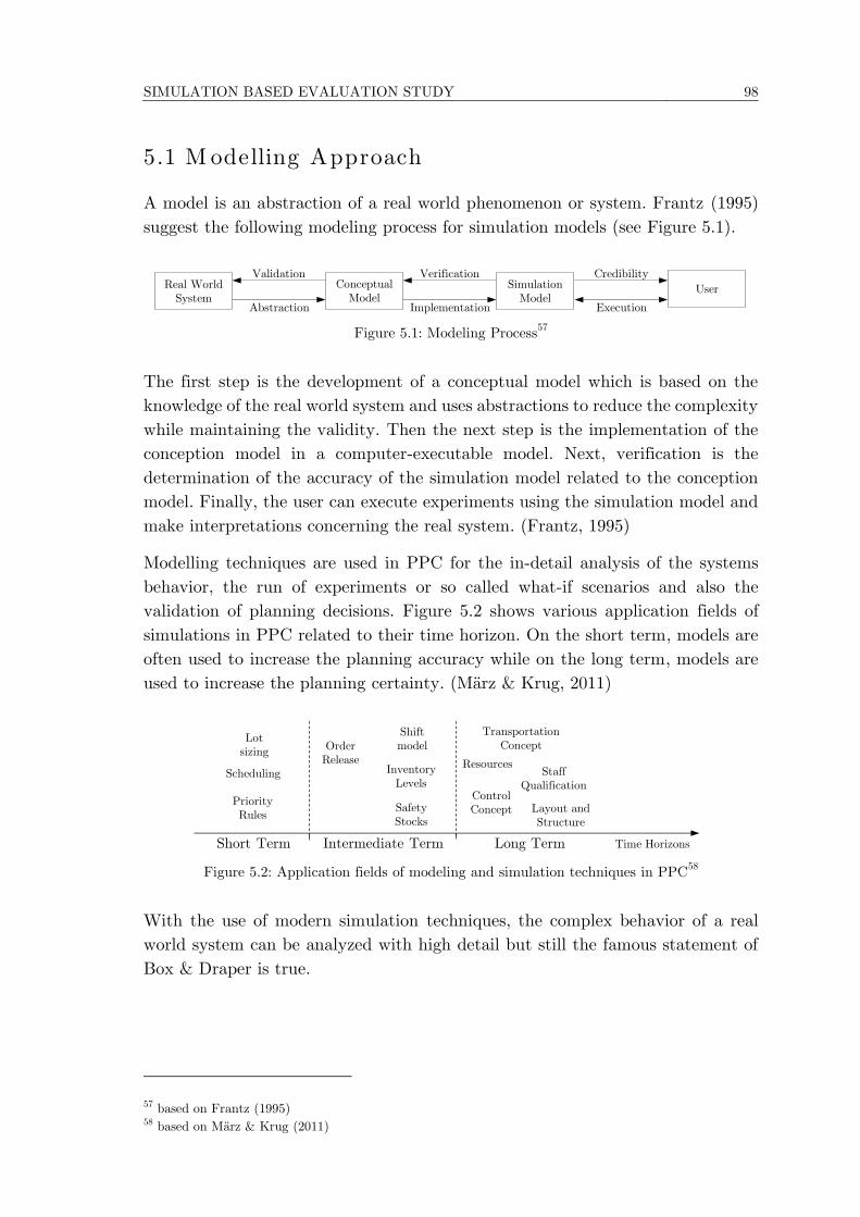
SIMULATION BASED EVALUATION STUDY 98
5.1 M odelling Approach
A model is an abstraction of a real world phenomenon or system. Frantz (1995)
suggest the following modeling process for simulation models (see Figure 5.1).
Figure 5.1: Modeling Process
57
The first step is the development of a conceptual model which is based on the
knowledge of the real world system and uses abstractions to reduce the complexity
while maintaining the validity. Then the next step is the implementation of the
conception model in a computer-executable model. Next, verification is the
determination of the accuracy of the simulation model related to the conception
model. Finally, the user can execute experiments using the simulation model and
make interpretations concerning the real system. (Frantz, 1995)
Modelling techniques are used in PPC for the in-detail analysis of the systems
behavior, the run of experiments or so called what-if scenarios and also the
validation of planning decisions. Figure 5.2 shows various application fields of
simulations in PPC related to their time horizon. On the short term, models are
often used to increase the planning accuracy while on the long term, models are
used to increase the planning certainty. (März & Krug, 2011)
Figure 5.2: Application fields of modeling and simulation techniques in PPC
58
With the use of modern simulation techniques, the complex behavior of a real
world system can be analyzed with high detail but still the famous statement of
Box & Draper is true.
57 based on Frantz (1995) 58 based on März & Krug (2011)
Real World System
UserSimulation Model
ConceptualModel
Validation
Abstraction
Verification
Implementation
Credibility
Execution
Short Term Intermediate Term Long Term
Transportation Concept
ResourcesStaff
QualificationControl Concept Layout and
Structure
Inventory Levels
Shift model
Safety Stocks
Order Release
Lot sizing
Scheduling
Priority Rules
Time Horizons
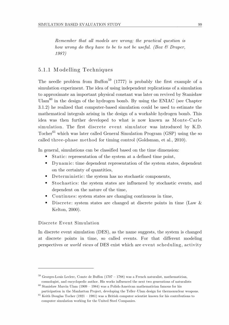
SIMULATION BASED EVALUATION STUDY 99
Remember that all models are wrong; the practical question is
how wrong do they have to be to not be useful. (Box & Draper,
1987)
5.1.1 M odelling Techniques
The needle problem from Buffon59 (1777) is probably the first example of a
simulation experiment. The idea of using independent replications of a simulation
to approximate an important physical constant was later on revived by Stanisław
Ulam60 in the design of the hydrogen bomb. By using the ENIAC (see Chapter
3.1.2) he realized that computer-based simulation could be used to estimate the
mathematical integrals arising in the design of a workable hydrogen bomb. This
idea was then further developed to what is now known as M onte-Carlo
simulation. The first discrete event simulator was introduced by K.D.
Tocher61 which was later called General Simulation Program (GSP) using the so
called three-phase method for timing control (Goldsman, et al., 2010).
In general, simulations can be classified based on the time dimension:
Static: representation of the system at a defined time point,
Dynamic: time dependent representation of the system states, dependent
on the certainty of quantities,
Deterministic: the system has no stochastic components,
Stochastics: the system states are influenced by stochastic events, and
dependent on the nature of the time,
Continues: system states are changing continuous in time,
Discrete: system states are changed at discrete points in time (Law &
Kelton, 2000).
Discrete Event Simulation
In discrete event simulation (DES), as the name suggests, the system is changed
at discrete points in time, so called events. For that different modeling
perspectives or world views of DES exist which are event scheduling, activity
59 Georges-Louis Leclerc, Comte de Buffon (1707 – 1788) was a French naturalist, mathematician,
cosmologist, and encyclopedic author. His works influenced the next two generations of naturalists 60 Stanisław Marcin Ulam (1909 – 1984) was a Polish-American mathematician famous for his
participation in the Manhattan Project, developing the Teller–Ulam design for thermonuclear weapons. 61 Keith Douglas Tocher (1921 – 1981) was a British computer scientist known for his contributions to
computer simulation working for the United Steel Companies.
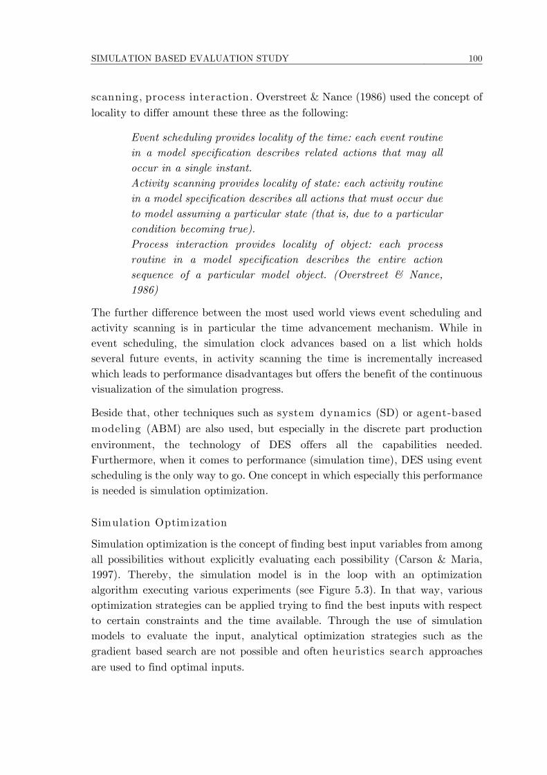
SIMULATION BASED EVALUATION STUDY 100
scanning, process interaction. Overstreet & Nance (1986) used the concept of
locality to differ amount these three as the following:
Event scheduling provides locality of the time: each event routine
in a model specification describes related actions that may all
occur in a single instant.
Activity scanning provides locality of state: each activity routine
in a model specification describes all actions that must occur due
to model assuming a particular state (that is, due to a particular
condition becoming true).
Process interaction provides locality of object: each process
routine in a model specification describes the entire action
sequence of a particular model object. (Overstreet & Nance,
1986)
The further difference between the most used world views event scheduling and
activity scanning is in particular the time advancement mechanism. While in
event scheduling, the simulation clock advances based on a list which holds
several future events, in activity scanning the time is incrementally increased
which leads to performance disadvantages but offers the benefit of the continuous
visualization of the simulation progress.
Beside that, other techniques such as system dynamics (SD) or agent-based
modeling (ABM) are also used, but especially in the discrete part production
environment, the technology of DES offers all the capabilities needed.
Furthermore, when it comes to performance (simulation time), DES using event
scheduling is the only way to go. One concept in which especially this performance
is needed is simulation optimization.
Simulation Optimization
Simulation optimization is the concept of finding best input variables from among
all possibilities without explicitly evaluating each possibility (Carson & Maria,
1997). Thereby, the simulation model is in the loop with an optimization
algorithm executing various experiments (see Figure 5.3). In that way, various
optimization strategies can be applied trying to find the best inputs with respect
to certain constraints and the time available. Through the use of simulation
models to evaluate the input, analytical optimization strategies such as the
gradient based search are not possible and often heuristics search approaches
are used to find optimal inputs.
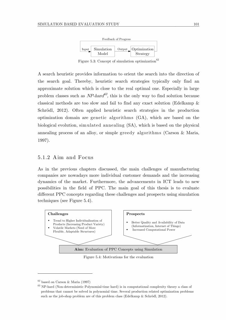
SIMULATION BASED EVALUATION STUDY 101
Figure 5.3: Concept of simulation optimization
62
A search heuristic provides information to orient the search into the direction of
the search goal. Thereby, heuristic search strategies typically only find an
approximate solution which is close to the real optimal one. Especially in large
problem classes such as NP-hard63, this is the only way to find solution because
classical methods are too slow and fail to find any exact solution (Edelkamp &
Schrödl, 2012). Often applied heuristic search strategies in the production
optimization domain are genetic algorithms (GA), which are based on the
biological evolution, simulated annealing (SA), which is based on the physical
annealing process of an alloy, or simple greedy algorithms (Carson & Maria,
1997).
5.1.2 Aim and Focus
As in the previous chapters discussed, the main challenges of manufacturing
companies are nowadays more individual customer demands and the increasing
dynamics of the market. Furthermore, the advancements in ICT leads to new
possibilities in the field of PPC. The main goal of this thesis is to evaluate
different PPC concepts regarding these challenges and prospects using simulation
techniques (see Figure 5.4).
Figure 5.4: Motivations for the evaluation
62 based on Carson & Maria (1997) 63 NP-hard (Non-deterministic Polynomial-time hard) is in computational complexity theory a class of
problems that cannot be solved in polynomial time. Several production related optimization problems
such as the job-shop problem are of this problem class (Edelkamp & Schrödl, 2012).
Simulation Model
OptimizationStrategy
OutputInput
Feedback of Progress
Challenges Prospects
Trend to Higher Individualization of Products (Increasing Product Variety)
Volatile Markets (Need of More Flexible, Adaptable Structures)
Better Quality and Availability of Data (Informatization, Internet of Things)
Increased Computational Power
Aim: Evaluation of PPC Concepts using Simulation
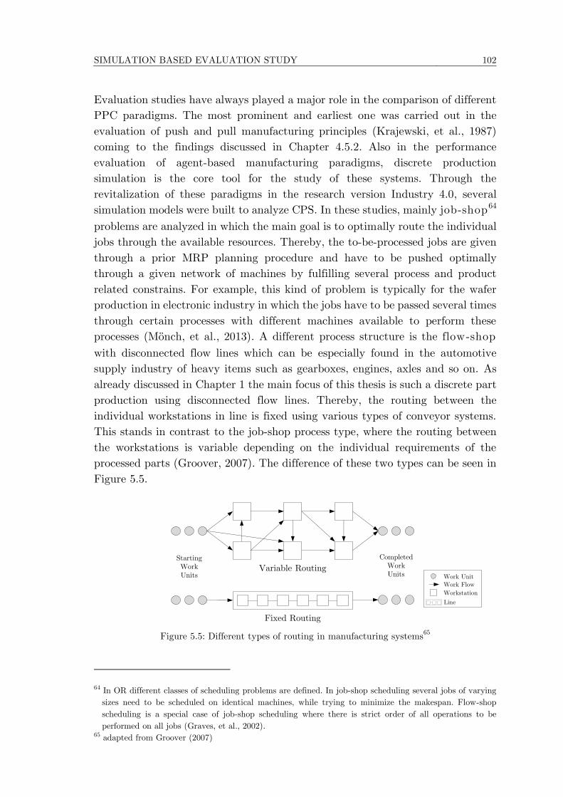
SIMULATION BASED EVALUATION STUDY 102
Evaluation studies have always played a major role in the comparison of different
PPC paradigms. The most prominent and earliest one was carried out in the
evaluation of push and pull manufacturing principles (Krajewski, et al., 1987)
coming to the findings discussed in Chapter 4.5.2. Also in the performance
evaluation of agent-based manufacturing paradigms, discrete production
simulation is the core tool for the study of these systems. Through the
revitalization of these paradigms in the research version Industry 4.0, several
simulation models were built to analyze CPS. In these studies, mainly job-shop64
problems are analyzed in which the main goal is to optimally route the individual
jobs through the available resources. Thereby, the to-be-processed jobs are given
through a prior MRP planning procedure and have to be pushed optimally
through a given network of machines by fulfilling several process and product
related constrains. For example, this kind of problem is typically for the wafer
production in electronic industry in which the jobs have to be passed several times
through certain processes with different machines available to perform these
processes (Mönch, et al., 2013). A different process structure is the flow-shop
with disconnected flow lines which can be especially found in the automotive
supply industry of heavy items such as gearboxes, engines, axles and so on. As
already discussed in Chapter 1 the main focus of this thesis is such a discrete part
production using disconnected flow lines. Thereby, the routing between the
individual workstations in line is fixed using various types of conveyor systems.
This stands in contrast to the job-shop process type, where the routing between
the workstations is variable depending on the individual requirements of the
processed parts (Groover, 2007). The difference of these two types can be seen in
Figure 5.5.
Figure 5.5: Different types of routing in manufacturing systems
65
64 In OR different classes of scheduling problems are defined. In job-shop scheduling several jobs of varying
sizes need to be scheduled on identical machines, while trying to minimize the makespan. Flow-shop
scheduling is a special case of job-shop scheduling where there is strict order of all operations to be
performed on all jobs (Graves, et al., 2002). 65 adapted from Groover (2007)
Workstation
Work Flow
Starting Work Units
Completed Work Units Work Unit
Variable Routing
Fixed Routing
Line
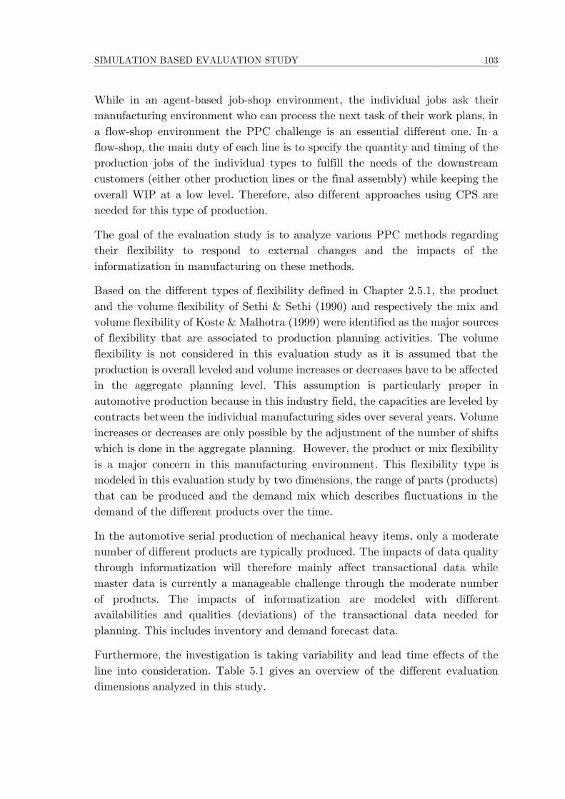
SIMULATION BASED EVALUATION STUDY 103
While in an agent-based job-shop environment, the individual jobs ask their
manufacturing environment who can process the next task of their work plans, in
a flow-shop environment the PPC challenge is an essential different one. In a
flow-shop, the main duty of each line is to specify the quantity and timing of the
production jobs of the individual types to fulfill the needs of the downstream
customers (either other production lines or the final assembly) while keeping the
overall WIP at a low level. Therefore, also different approaches using CPS are
needed for this type of production.
The goal of the evaluation study is to analyze various PPC methods regarding
their flexibility to respond to external changes and the impacts of the
informatization in manufacturing on these methods.
Based on the different types of flexibility defined in Chapter 2.5.1, the product
and the volume flexibility of Sethi & Sethi (1990) and respectively the mix and
volume flexibility of Koste & Malhotra (1999) were identified as the major sources
of flexibility that are associated to production planning activities. The volume
flexibility is not considered in this evaluation study as it is assumed that the
production is overall leveled and volume increases or decreases have to be affected
in the aggregate planning level. This assumption is particularly proper in
automotive production because in this industry field, the capacities are leveled by
contracts between the individual manufacturing sides over several years. Volume
increases or decreases are only possible by the adjustment of the number of shifts
which is done in the aggregate planning. However, the product or mix flexibility
is a major concern in this manufacturing environment. This flexibility type is
modeled in this evaluation study by two dimensions, the range of parts (products)
that can be produced and the demand mix which describes fluctuations in the
demand of the different products over the time.
In the automotive serial production of mechanical heavy items, only a moderate
number of different products are typically produced. The impacts of data quality
through informatization will therefore mainly affect transactional data while
master data is currently a manageable challenge through the moderate number
of products. The impacts of informatization are modeled with different
availabilities and qualities (deviations) of the transactional data needed for
planning. This includes inventory and demand forecast data.
Furthermore, the investigation is taking variability and lead time effects of the
line into consideration. Table 5.1 gives an overview of the different evaluation
dimensions analyzed in this study.
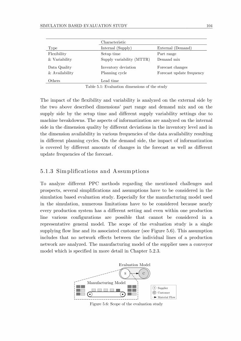
SIMULATION BASED EVALUATION STUDY 104
Characteristic
Type Internal (Supply) External (Demand)
Flexibility
& Variability
Setup time
Supply variability (MTTR)
Part range
Demand mix
Data Quality
& Availability
Inventory deviation
Planning cycle
Forecast changes
Forecast update frequency
Others Lead time
Table 5.1: Evaluation dimensions of the study
The impact of the flexibility and variability is analyzed on the external side by
the two above described dimensions’ part range and demand mix and on the
supply side by the setup time and different supply variability settings due to
machine breakdowns. The aspects of informatization are analyzed on the internal
side in the dimension quality by different deviations in the inventory level and in
the dimension availability in various frequencies of the data availability resulting
in different planning cycles. On the demand side, the impact of informatization
is covered by different amounts of changes in the forecast as well as different
update frequencies of the forecast.
5.1.3 Simplifications and Assumptions
To analyze different PPC methods regarding the mentioned challenges and
prospects, several simplifications and assumptions have to be considered in the
simulation based evaluation study. Especially for the manufacturing model used
in the simulation, numerous limitations have to be considered because nearly
every production system has a different setting and even within one production
line various configurations are possible that cannot be considered in a
representative general model. The scope of the evaluation study is a single
supplying flow line and its associated customer (see Figure 5.6). This assumption
includes that no network effects between the individual lines of a production
network are analyzed. The manufacturing model of the supplier uses a conveyor
model which is specified in more detail in Chapter 5.2.3.
Figure 5.6: Scope of the evaluation study
C
Manufacturing Model
S
Evaluation Model
S
C
Supplier
Customer
Material Flow
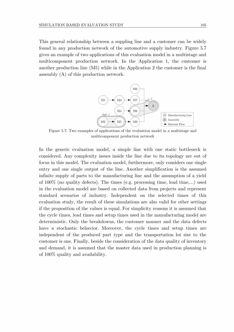
SIMULATION BASED EVALUATION STUDY 105
This general relationship between a suppling line and a customer can be widely
found in any production network of the automotive supply industry. Figure 5.7
gives an example of two applications of this evaluation model in a multistage and
multicomponent production network. In the Application 1, the customer is
another production line (M5) while in the Application 2 the customer is the final
assembly (A) of this production network.
Figure 5.7: Two examples of applications of the evaluation model in a multistage and
multicomponent production network
In the generic evaluation model, a simple line with one static bottleneck is
considered. Any complexity issues inside the line due to its topology are out of
focus in this model. The evaluation model, furthermore, only considers one single
entry and one single output of the line. Another simplification is the assumed
infinite supply of parts to the manufacturing line and the assumption of a yield
of 100% (no quality defects). The times (e.g. processing time, lead time,…) used
in the evaluation model are based on collected data from projects and represent
standard scenarios of industry. Independent on the selected times of this
evaluation study, the result of these simulations are also valid for other settings
if the proposition of the values is equal. For simplicity reasons it is assumed that
the cycle times, lead times and setup times used in the manufacturing model are
deterministic. Only the breakdowns, the customer manner and the data defects
have a stochastic behavior. Moreover, the cycle times and setup times are
independent of the produced part type and the transportation lot size to the
customer is one. Finally, beside the consideration of the data quality of inventory
and demand, it is assumed that the master data used in production planning is
of 100% quality and availability.
A
M7
M8
M9
M6
M3
M4
M5
M
A
Manufacturing Line
Assembly
Material Flow
M1
M2
Appl. 1
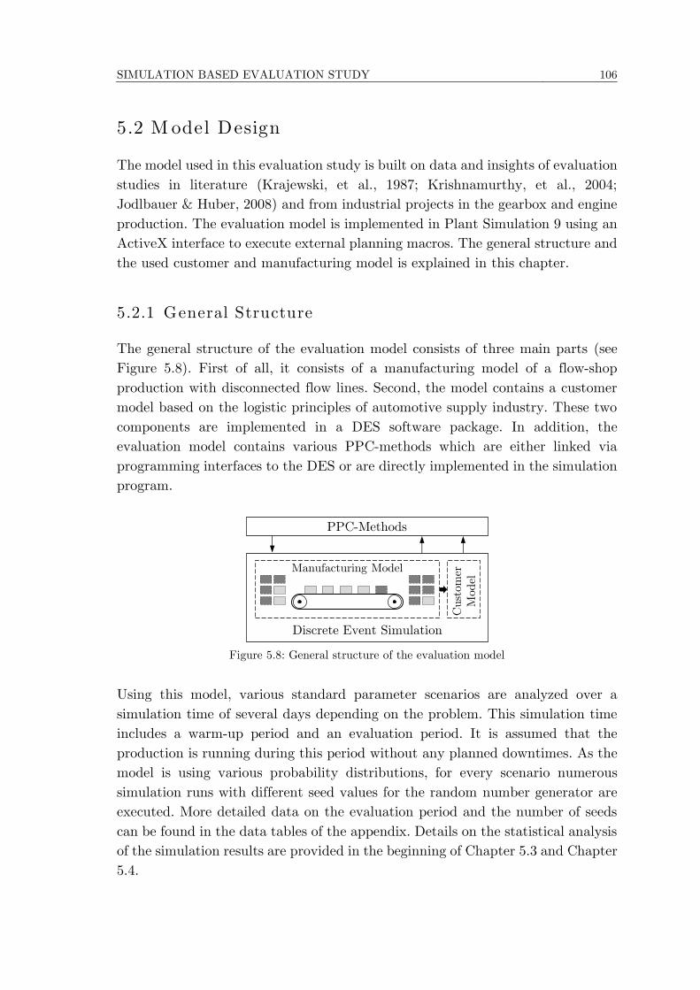
SIMULATION BASED EVALUATION STUDY 106
5.2 M odel Design
The model used in this evaluation study is built on data and insights of evaluation
studies in literature (Krajewski, et al., 1987; Krishnamurthy, et al., 2004;
Jodlbauer & Huber, 2008) and from industrial projects in the gearbox and engine
production. The evaluation model is implemented in Plant Simulation 9 using an
ActiveX interface to execute external planning macros. The general structure and
the used customer and manufacturing model is explained in this chapter.
5.2.1 General Structure
The general structure of the evaluation model consists of three main parts (see
Figure 5.8). First of all, it consists of a manufacturing model of a flow-shop
production with disconnected flow lines. Second, the model contains a customer
model based on the logistic principles of automotive supply industry. These two
components are implemented in a DES software package. In addition, the
evaluation model contains various PPC-methods which are either linked via
programming interfaces to the DES or are directly implemented in the simulation
program.
Figure 5.8: General structure of the evaluation model
Using this model, various standard parameter scenarios are analyzed over a
simulation time of several days depending on the problem. This simulation time
includes a warm-up period and an evaluation period. It is assumed that the
production is running during this period without any planned downtimes. As the
model is using various probability distributions, for every scenario numerous
simulation runs with different seed values for the random number generator are
executed. More detailed data on the evaluation period and the number of seeds
can be found in the data tables of the appendix. Details on the statistical analysis
of the simulation results are provided in the beginning of Chapter 5.3 and Chapter
5.4.
Manufacturing Model
Discrete Event Simulation
Cust
omer
Mod
el
PPC-Methods
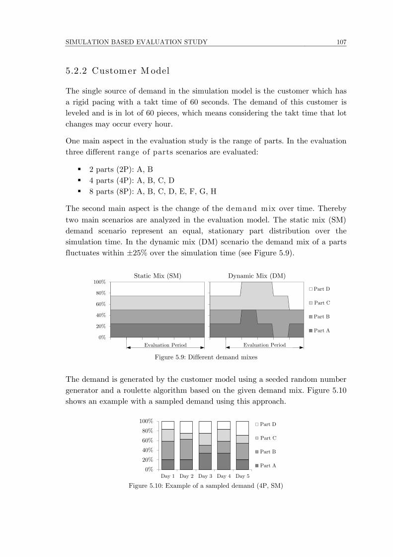
SIMULATION BASED EVALUATION STUDY 107
5.2.2 Customer M odel
The single source of demand in the simulation model is the customer which has
a rigid pacing with a takt time of 60 seconds. The demand of this customer is
leveled and is in lot of 60 pieces, which means considering the takt time that lot
changes may occur every hour.
One main aspect in the evaluation study is the range of parts. In the evaluation
three different range of parts scenarios are evaluated:
2 parts (2P): A, B
4 parts (4P): A, B, C, D
8 parts (8P): A, B, C, D, E, F, G, H
The second main aspect is the change of the demand mix over time. Thereby
two main scenarios are analyzed in the evaluation model. The static mix (SM)
demand scenario represent an equal, stationary part distribution over the
simulation time. In the dynamic mix (DM) scenario the demand mix of a parts
fluctuates within ±25% over the simulation time (see Figure 5.9).
Figure 5.9: Different demand mixes
The demand is generated by the customer model using a seeded random number
generator and a roulette algorithm based on the given demand mix. Figure 5.10
shows an example with a sampled demand using this approach.
Figure 5.10: Example of a sampled demand (4P, SM)
0%
20%
40%
60%
80%
100%
Product D
Product C
Product B
Product A
0%
20%
40%
60%
80%
100%
Product D
Product C
Product B
Product A
Evaluation Period Evaluation Period
Static Mix (SM) Dynamic Mix (DM)
Part D
Part C
Part B
Part A
0%
20%
40%
60%
80%
100%
Day 1 Day 2 Day 3 Day 4 Day 50%
20%
40%
60%
80%
100%
Product D
Product C
Product B
Product A
Part D
Part C
Part B
Part A
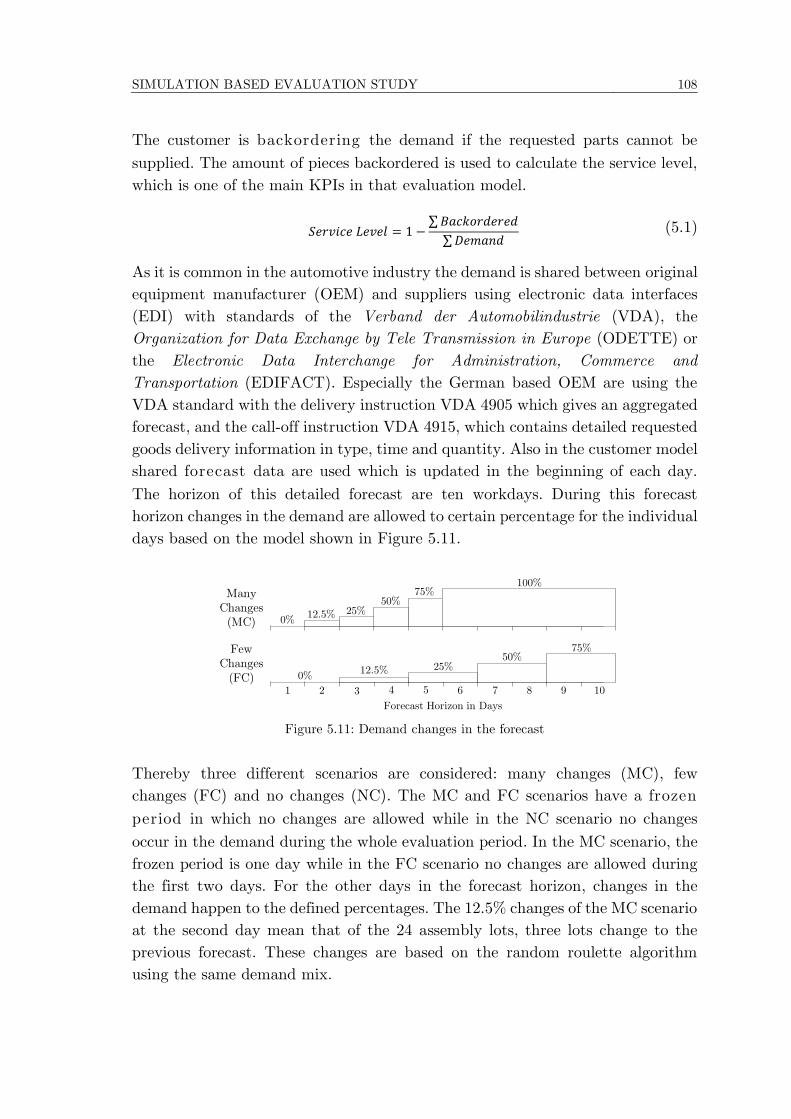
SIMULATION BASED EVALUATION STUDY 108
The customer is backordering the demand if the requested parts cannot be
supplied. The amount of pieces backordered is used to calculate the service level,
which is one of the main KPIs in that evaluation model.
𝑆𝑒𝑟𝑣𝑖𝑐𝑒 𝐿𝑒𝑣𝑒𝑙 = 1 −∑ 𝐵𝑎𝑐𝑘𝑜𝑟𝑑𝑒𝑟𝑒𝑑
∑ 𝐷𝑒𝑚𝑎𝑛𝑑 (5.1)
As it is common in the automotive industry the demand is shared between original
equipment manufacturer (OEM) and suppliers using electronic data interfaces
(EDI) with standards of the Verband der Automobilindustrie (VDA), the
Organization for Data Exchange by Tele Transmission in Europe (ODETTE) or
the Electronic Data Interchange for Administration, Commerce and
Transportation (EDIFACT). Especially the German based OEM are using the
VDA standard with the delivery instruction VDA 4905 which gives an aggregated
forecast, and the call-off instruction VDA 4915, which contains detailed requested
goods delivery information in type, time and quantity. Also in the customer model
shared forecast data are used which is updated in the beginning of each day.
The horizon of this detailed forecast are ten workdays. During this forecast
horizon changes in the demand are allowed to certain percentage for the individual
days based on the model shown in Figure 5.11.
Figure 5.11: Demand changes in the forecast
Thereby three different scenarios are considered: many changes (MC), few
changes (FC) and no changes (NC). The MC and FC scenarios have a frozen
period in which no changes are allowed while in the NC scenario no changes
occur in the demand during the whole evaluation period. In the MC scenario, the
frozen period is one day while in the FC scenario no changes are allowed during
the first two days. For the other days in the forecast horizon, changes in the
demand happen to the defined percentages. The 12.5% changes of the MC scenario
at the second day mean that of the 24 assembly lots, three lots change to the
previous forecast. These changes are based on the random roulette algorithm
using the same demand mix.
1 2 3 4 5 6
Forecast Horizon in Days
7 8 9 10
FewChanges
(FC)
75%
0%12.5% 25%
50%
100%75%
0%12.5% 25%
50%Many
Changes(MC)
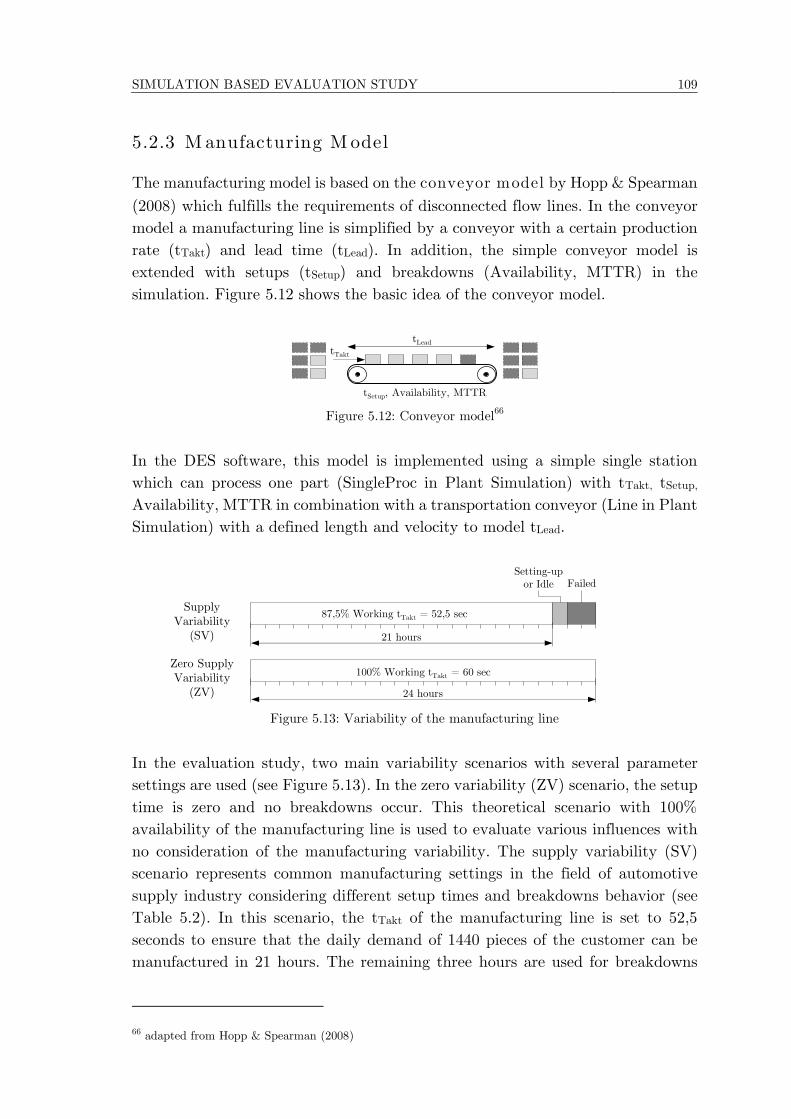
SIMULATION BASED EVALUATION STUDY 109
5.2.3 M anufacturing M odel
The manufacturing model is based on the conveyor model by Hopp & Spearman
(2008) which fulfills the requirements of disconnected flow lines. In the conveyor
model a manufacturing line is simplified by a conveyor with a certain production
rate (tTakt) and lead time (tLead). In addition, the simple conveyor model is
extended with setups (tSetup) and breakdowns (Availability, MTTR) in the
simulation. Figure 5.12 shows the basic idea of the conveyor model.
Figure 5.12: Conveyor model
66
In the DES software, this model is implemented using a simple single station
which can process one part (SingleProc in Plant Simulation) with tTakt, tSetup,
Availability, MTTR in combination with a transportation conveyor (Line in Plant
Simulation) with a defined length and velocity to model tLead.
Figure 5.13: Variability of the manufacturing line
In the evaluation study, two main variability scenarios with several parameter
settings are used (see Figure 5.13). In the zero variability (ZV) scenario, the setup
time is zero and no breakdowns occur. This theoretical scenario with 100%
availability of the manufacturing line is used to evaluate various influences with
no consideration of the manufacturing variability. The supply variability (SV)
scenario represents common manufacturing settings in the field of automotive
supply industry considering different setup times and breakdowns behavior (see
Table 5.2). In this scenario, the tTakt of the manufacturing line is set to 52,5
seconds to ensure that the daily demand of 1440 pieces of the customer can be
manufactured in 21 hours. The remaining three hours are used for breakdowns
66 adapted from Hopp & Spearman (2008)
tLead
tTakt
tSetup, Availability, MTTR
100% Working tTakt = 60 sec
87,5% Working tTakt = 52,5 sec
24 hours
21 hours
Setting-upor Idle Failed
Zero SupplyVariability
(ZV)
SupplyVariability
(SV)
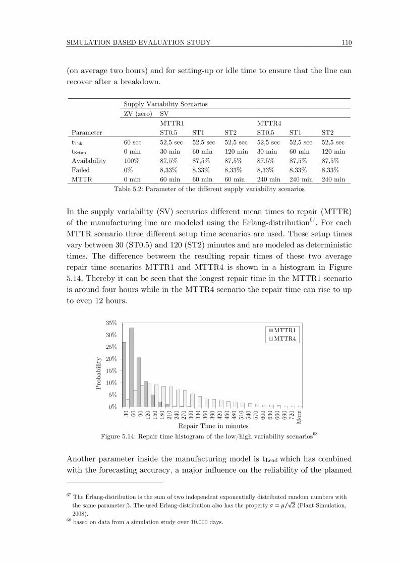
SIMULATION BASED EVALUATION STUDY 110
(on average two hours) and for setting-up or idle time to ensure that the line can
recover after a breakdown.
Supply Variability Scenarios
ZV (zero) SV
MTTR1 MTTR4
Parameter ST0.5 ST1 ST2 ST0,5 ST1 ST2
tTakt 60 sec 52,5 sec 52,5 sec 52,5 sec 52,5 sec 52,5 sec 52,5 sec
tSetup 0 min 30 min 60 min 120 min 30 min 60 min 120 min
Availability 100% 87,5% 87,5% 87,5% 87,5% 87,5% 87,5%
Failed 0% 8,33% 8,33% 8,33% 8,33% 8,33% 8,33%
MTTR 0 min 60 min 60 min 60 min 240 min 240 min 240 min
Table 5.2: Parameter of the different supply variability scenarios
In the supply variability (SV) scenarios different mean times to repair (MTTR)
of the manufacturing line are modeled using the Erlang-distribution67. For each
MTTR scenario three different setup time scenarios are used. These setup times
vary between 30 (ST0.5) and 120 (ST2) minutes and are modeled as deterministic
times. The difference between the resulting repair times of these two average
repair time scenarios MTTR1 and MTTR4 is shown in a histogram in Figure
5.14. Thereby it can be seen that the longest repair time in the MTTR1 scenario
is around four hours while in the MTTR4 scenario the repair time can rise to up
to even 12 hours.
Figure 5.14: Repair time histogram of the low/high variability scenarios
68
Another parameter inside the manufacturing model is tLead which has combined
with the forecasting accuracy, a major influence on the reliability of the planned
67 The Erlang-distribution is the sum of two independent exponentially distributed random numbers with
the same parameter β. The used Erlang-distribution also has the property 𝜎 = 𝜇 √2⁄ (Plant Simulation,
2008). 68 based on data from a simulation study over 10.000 days.
0%
5%
10%
15%
20%
25%
30%
35%
30 60
90
120
150
180
210
240
270
300
330
360
390
420
450
480
510
540
570
600 630
660
690
720
Mor
e
Pro
bability
Repair Time in minutes
MTTR1
MTTR4
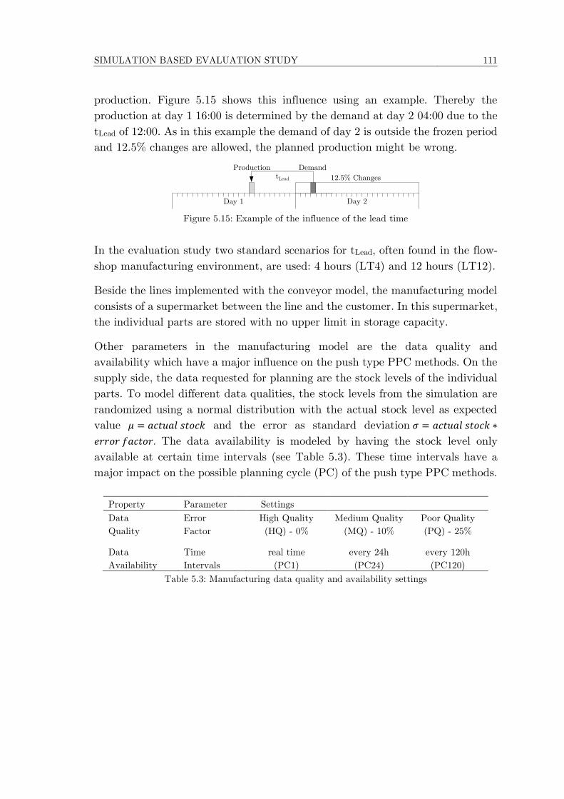
SIMULATION BASED EVALUATION STUDY 111
production. Figure 5.15 shows this influence using an example. Thereby the
production at day 1 16:00 is determined by the demand at day 2 04:00 due to the
tLead of 12:00. As in this example the demand of day 2 is outside the frozen period
and 12.5% changes are allowed, the planned production might be wrong.
Figure 5.15: Example of the influence of the lead time
In the evaluation study two standard scenarios for tLead, often found in the flow-
shop manufacturing environment, are used: 4 hours (LT4) and 12 hours (LT12).
Beside the lines implemented with the conveyor model, the manufacturing model
consists of a supermarket between the line and the customer. In this supermarket,
the individual parts are stored with no upper limit in storage capacity.
Other parameters in the manufacturing model are the data quality and
availability which have a major influence on the push type PPC methods. On the
supply side, the data requested for planning are the stock levels of the individual
parts. To model different data qualities, the stock levels from the simulation are
randomized using a normal distribution with the actual stock level as expected
value 𝜇 = 𝑎𝑐𝑡𝑢𝑎𝑙 𝑠𝑡𝑜𝑐𝑘 and the error as standard deviation 𝜎 = 𝑎𝑐𝑡𝑢𝑎𝑙 𝑠𝑡𝑜𝑐𝑘 ∗
𝑒𝑟𝑟𝑜𝑟 𝑓𝑎𝑐𝑡𝑜𝑟. The data availability is modeled by having the stock level only
available at certain time intervals (see Table 5.3). These time intervals have a
major impact on the possible planning cycle (PC) of the push type PPC methods.
Property Parameter Settings
Data
Quality
Error
Factor
High Quality
(HQ) - 0%
Medium Quality
(MQ) - 10%
Poor Quality
(PQ) - 25%
Data
Availability
Time
Intervals
real time
(PC1)
every 24h
(PC24)
every 120h
(PC120)
Table 5.3: Manufacturing data quality and availability settings
12.5% ChangestLead
Day 1 Day 2
DemandProduction
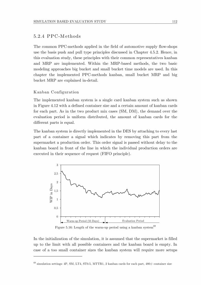
SIMULATION BASED EVALUATION STUDY 112
5.2.4 PPC-M ethods
The common PPC-methods applied in the field of automotive supply flow-shops
use the basis push and pull type principles discussed in Chapter 4.5.2. Hence, in
this evaluation study, these principles with their common representatives kanban
and MRP are implemented. Within the MRP-based methods, the two basic
modeling approaches big bucket and small bucket time models are used. In this
chapter the implemented PPC-methods kanban, small bucket MRP and big
bucket MRP are explained in-detail.
Kanban Configuration
The implemented kanban system is a single card kanban system such as shown
in Figure 4.12 with a defined container size and a certain amount of kanban cards
for each part. As in the two product mix cases (SM, DM), the demand over the
evaluation period is uniform distributed, the amount of kanban cards for the
different parts is equal.
The kanban system is directly implemented in the DES by attaching to every last
part of a container a signal which indicates by removing this part from the
supermarket a production order. This order signal is passed without delay to the
kanban board in front of the line in which the individual production orders are
executed in their sequence of request (FIFO principle).
Figure 5.16: Length of the warm-up period using a kanban system
69
In the initialization of the simulation, it is assumed that the supermarket is filled
up to the limit with all possible containers and the kanban board is empty. In
case of a too small container sizes the kanban system will require more setups
69 simulation settings: 4P, SM, LT4, ST0.5, MTTR1, 2 kanban cards for each part, 480# container size
0
0,5
1
1,5
2
2,5
3
WIP
in D
ays
Warm-up Period (55 Days) Evaluation Period
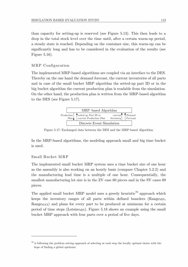
SIMULATION BASED EVALUATION STUDY 113
than capacity for setting-up is reserved (see Figure 5.13). This then leads to a
drop in the total stock level over the time until, after a certain warm-up period,
a steady state is reached. Depending on the container size, this warm-up can be
significantly long and has to be considered in the evaluation of the results (see
Figure 5.16).
M RP Configuration
The implemented MRP-based algorithms are coupled via an interface to the DES.
Thereby on the one hand the demand forecast, the current inventories of all parts
and in case of the small bucket MRP algorithm the setted-up part ID or in the
big bucket algorithm the current production plan is readable from the simulation.
On the other hand, the production plan is written from the MRP-based algorithm
to the DES (see Figure 5.17).
Figure 5.17: Exchanged data between the DES and the MRP-based Algorithm
In the MRP-based algorithms, the modeling approach small and big time bucket
is used.
Small Bucket M RP
The implemented small bucket MRP system uses a time bucket size of one hour
as the assembly is also working on an hourly basis (compare Chapter 5.2.2) and
the manufacturing lead time is a multiple of one hour. Consequentially, the
smallest manufacturing lot size is in the ZV case 60 pieces and in the SV cases 69
pieces.
The applied small bucket MRP model uses a greedy heuristic70 approach which
keeps the inventory ranges of all parts within defined boarders (RangeMIN,
RangeMAX) and plans for every part to be produced at minimum for a certain
period of time steps (LotsizeMIN). Figure 5.18 shows an example using the small
bucket MRP approach with four parts over a period of five days.
70 is following the problem solving approach of selecting at each step the locally optimal choice with the
hope of finding a global optimum
MRP–based Algorithm
Demand Forecast
current Inventory
ProductionPlan
setted up Part ID orcurrent Production Plan
Discrete Event Simulation
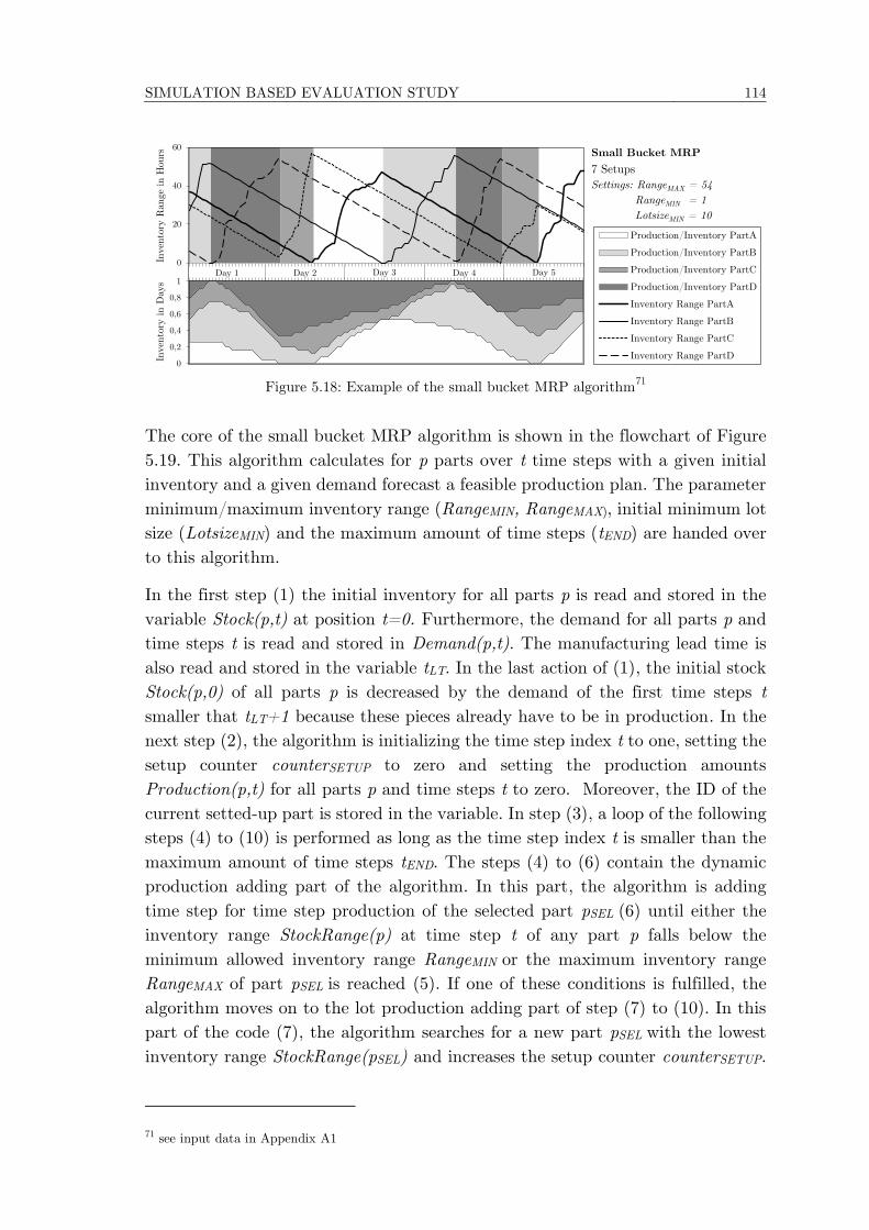
SIMULATION BASED EVALUATION STUDY 114
Figure 5.18: Example of the small bucket MRP algorithm
71
The core of the small bucket MRP algorithm is shown in the flowchart of Figure
5.19. This algorithm calculates for p parts over t time steps with a given initial
inventory and a given demand forecast a feasible production plan. The parameter
minimum/maximum inventory range (RangeMIN, RangeMAX), initial minimum lot
size (LotsizeMIN) and the maximum amount of time steps (tEND) are handed over
to this algorithm.
In the first step (1) the initial inventory for all parts p is read and stored in the
variable Stock(p,t) at position t=0. Furthermore, the demand for all parts p and
time steps t is read and stored in Demand(p,t). The manufacturing lead time is
also read and stored in the variable tLT. In the last action of (1), the initial stock
Stock(p,0) of all parts p is decreased by the demand of the first time steps t
smaller that tLT+1 because these pieces already have to be in production. In the
next step (2), the algorithm is initializing the time step index t to one, setting the
setup counter counterSETUP to zero and setting the production amounts
Production(p,t) for all parts p and time steps t to zero. Moreover, the ID of the
current setted-up part is stored in the variable. In step (3), a loop of the following
steps (4) to (10) is performed as long as the time step index t is smaller than the
maximum amount of time steps tEND. The steps (4) to (6) contain the dynamic
production adding part of the algorithm. In this part, the algorithm is adding
time step for time step production of the selected part pSEL (6) until either the
inventory range StockRange(p) at time step t of any part p falls below the
minimum allowed inventory range RangeMIN or the maximum inventory range
RangeMAX of part pSEL is reached (5). If one of these conditions is fulfilled, the
algorithm moves on to the lot production adding part of step (7) to (10). In this
part of the code (7), the algorithm searches for a new part pSEL with the lowest
inventory range StockRange(pSEL) and increases the setup counter counterSETUP.
71 see input data in Appendix A1
0
20
40
60
0
0,2
0,4
0,6
0,8
1Day 1 Day 2 Day 3 Day 4 Day 5
0
20
40
60
80
100
120
140
Production/Inventory PartA
Production/Inventory PartB
Production/Inventory PartC
Production/Inventory PartD
Inventory Range PartA
Inventory Range PartB
Inventory Range PartC
Inventory Range PartD
Small Bucket MRP
7 Setups
Settings: RangeMAX = 54
RangeMIN = 1
LotsizeMIN = 10
Inven
tory
Ran
ge
in H
ours
Inven
tory
in D
ays
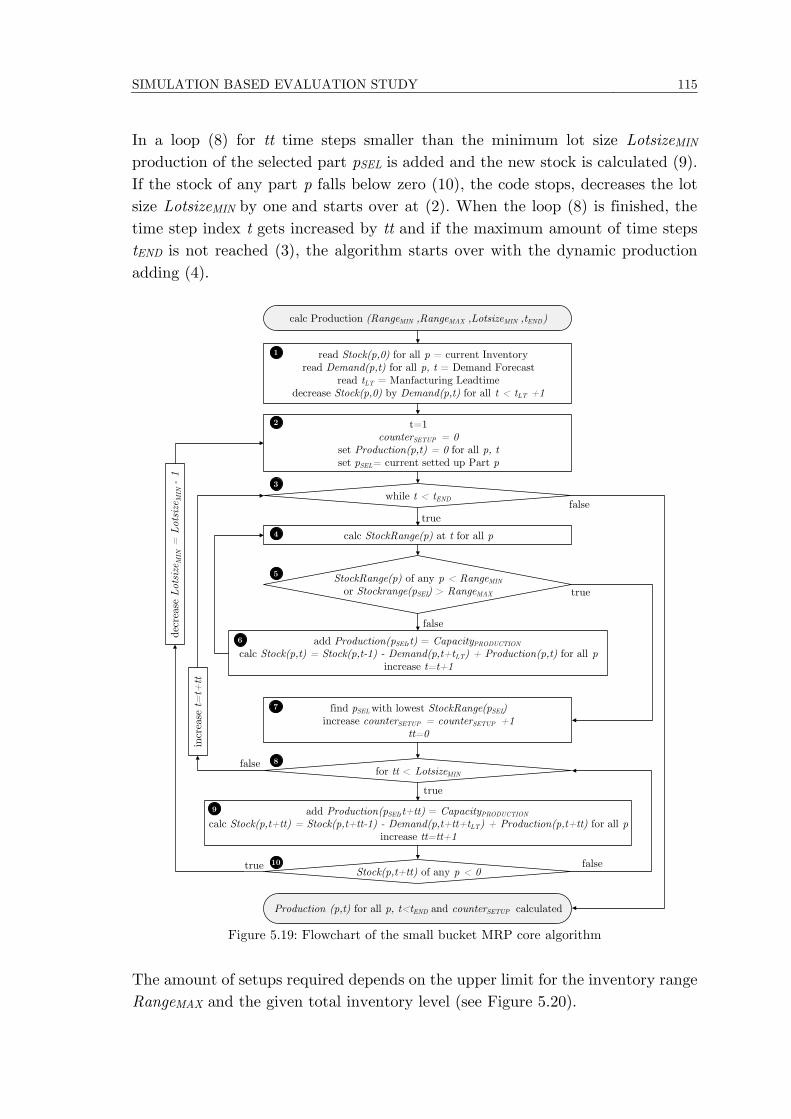
SIMULATION BASED EVALUATION STUDY 115
In a loop (8) for tt time steps smaller than the minimum lot size LotsizeMIN
production of the selected part pSEL is added and the new stock is calculated (9).
If the stock of any part p falls below zero (10), the code stops, decreases the lot
size LotsizeMIN by one and starts over at (2). When the loop (8) is finished, the
time step index t gets increased by tt and if the maximum amount of time steps
tEND is not reached (3), the algorithm starts over with the dynamic production
adding (4).
Figure 5.19: Flowchart of the small bucket MRP core algorithm
The amount of setups required depends on the upper limit for the inventory range
RangeMAX and the given total inventory level (see Figure 5.20).
t=1counterSETUP = 0
set Production(p,t) = 0 for all p, tset pSEL= current setted up Part p
calc StockRange(p) at t for all p
StockRange(p) of any p < RangeMIN
or Stockrange(pSEL) > RangeMAX
add Production(pSEL,t) = CapacityPRODUCTION
calc Stock(p,t) = Stock(p,t-1) - Demand(p,t+tLT) + Production(p,t) for all pincrease t=t+1
false
find pSEL with lowest StockRange(pSEL)increase counterSETUP = counterSETUP +1
tt=0
true
for tt < LotsizeMIN
add Production(pSEL,t+tt) = CapacityPRODUCTION
calc Stock(p,t+tt) = Stock(p,t+tt-1) - Demand(p,t+tt+tLT) + Production(p,t+tt) for all pincrease tt=tt+1
Stock(p,t+tt) of any p < 0
true
true
while t < tEND
true
Production (p,t) for all p, t<tEND and counterSETUP calculated
false
calc Production (RangeMIN ,RangeMAX ,LotsizeMIN ,tEND)
false
read Stock(p,0) for all p = current Inventory read Demand(p,t) for all p, t = Demand Forecast
read tLT = Manfacturing Leadtimedecrease Stock(p,0) by Demand(p,t) for all t < tLT +1
false
1
2
3
4
5
6
7
8
9
10
incr
ease
t=
t+tt
dec
reas
e Lots
ize M
IN=
Lots
ize M
IN-
1
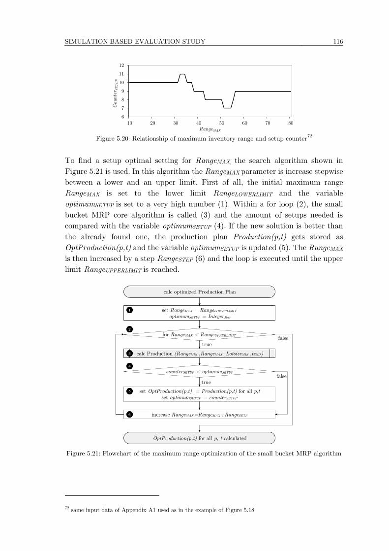
SIMULATION BASED EVALUATION STUDY 116
Figure 5.20: Relationship of maximum inventory range and setup counter
72
To find a setup optimal setting for RangeMAX, the search algorithm shown in
Figure 5.21 is used. In this algorithm the RangeMAX parameter is increase stepwise
between a lower and an upper limit. First of all, the initial maximum range
RangeMAX is set to the lower limit RangeLOWERLIMIT and the variable
optimumSETUP is set to a very high number (1). Within a for loop (2), the small
bucket MRP core algorithm is called (3) and the amount of setups needed is
compared with the variable optimumSETUP (4). If the new solution is better than
the already found one, the production plan Production(p,t) gets stored as
OptProduction(p,t) and the variable optimumSETUP is updated (5). The RangeMAX
is then increased by a step RangeSTEP (6) and the loop is executed until the upper
limit RangeUPPERLIMIT is reached.
Figure 5.21: Flowchart of the maximum range optimization of the small bucket MRP algorithm
72 same input data of Appendix A1 used as in the example of Figure 5.18
6
7
8
9
10
11
12
10 20 30 40 50 60 70 80
Counte
r SETU
P
RangeMAX
calc optimized Production Plan
for RangeMAX < RangeUPPERLIMIT
set RangeMAX = RangeLOWERLIMIT
optimumSETUP = IntegerMax
increase RangeMAX=RangeMAX+RangeSETP
set OptProduction(p,t) = Production(p,t) for all p,tset optimumSETUP = counterSETUP
counterSETUP < optimumSETUP
truefalse
calc Production (RangeMIN ,RangeMAX ,LotsizeMIN ,tEND)
true
OptProduction(p,t) for all p, t calculated
false
1
2
3
4
5
6
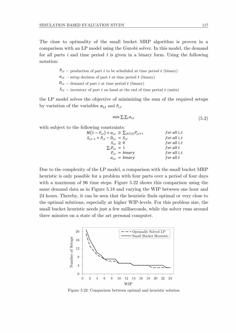
SIMULATION BASED EVALUATION STUDY 117
The close to optimality of the small bucket MRP algorithm is proven in a
comparison with an LP model using the Gurobi solver. In this model, the demand
for all parts i and time period t is given in a binary form. Using the following
notation:
𝑃𝑖,𝑡 = production of part 𝑖 to be scheduled at time period 𝑡 (binary)
𝛼𝑖,𝑡 = setup decision of part 𝑖 at time period 𝑡 (binary)
𝐷𝑖,𝑡 = demand of part 𝑖 at time period 𝑡 (binary)
𝑆𝑖,𝑡 = inventory of part 𝑖 on hand at the end of time period 𝑡 (units)
the LP model solves the objective of minimizing the sum of the required setups
by variation of the variables 𝛼𝑖,𝑡 and 𝑃𝑖,𝑡.
𝑚𝑖𝑛 ∑𝑖∑𝑡𝛼𝑖,𝑡 (5.2)
with subject to the following constraints: 𝑀(1 − 𝑃𝑖,𝑡) + 𝛼𝑖,𝑡 ≥ ∑𝑗∈𝐼\{𝑖}𝑃𝑗,𝑡+1 𝑓𝑜𝑟 𝑎𝑙𝑙 𝑖, 𝑡
𝑆𝑖,𝑡−1 + 𝑃𝑖,𝑡 − 𝐷𝑖,𝑡 = 𝑆𝑖,𝑡 𝑓𝑜𝑟 𝑎𝑙𝑙 𝑖, 𝑡
𝑆𝑖,𝑡 ≥ 0 𝑓𝑜𝑟 𝑎𝑙𝑙 𝑖, 𝑡
∑𝑖𝑃𝑖,𝑡 = 1 𝑓𝑜𝑟 𝑎𝑙𝑙 𝑡
𝑃𝑖,𝑡 = 𝑏𝑖𝑛𝑎𝑟𝑦 𝑓𝑜𝑟 𝑎𝑙𝑙 𝑖, 𝑡
𝛼𝑖,𝑡 = 𝑏𝑖𝑛𝑎𝑟𝑦 𝑓𝑜𝑟 𝑎𝑙𝑙 𝑡
Due to the complexity of the LP model, a comparison with the small bucket MRP
heuristic is only possible for a problem with four parts over a period of four days
with a maximum of 96 time steps. Figure 5.22 shows this comparison using the
same demand data as in Figure 5.18 and varying the WIP between one hour and
24 hours. Thereby, it can be seen that the heuristic finds optimal or very close to
the optimal solutions, especially at higher WIP-levels. For this problem size, the
small bucket heuristic needs just a few milliseconds, while the solver runs around
three minutes on a state of the art personal computer.
Figure 5.22: Comparison between optimal and heuristic solution
0
4
8
12
16
20
0 2 4 6 8 10 12 14 16 18 20 22 24
Num
ber
of Set
ups
WIP
Optimally Solved LPSmall Bucket Heuristic
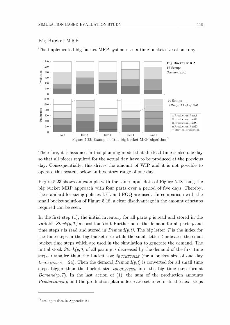
SIMULATION BASED EVALUATION STUDY 118
Big Bucket M RP
The implemented big bucket MRP system uses a time bucket size of one day.
Figure 5.23: Example of the big bucket MRP algorithm
73
Therefore, it is assumed in this planning model that the lead time is also one day
so that all pieces required for the actual day have to be produced at the previous
day. Consequentially, this drives the amount of WIP and it is not possible to
operate this system below an inventory range of one day.
Figure 5.23 shows an example with the same input data of Figure 5.18 using the
big bucket MRP approach with four parts over a period of five days. Thereby,
the standard lot-sizing policies LFL and FOQ are used. In comparison with the
small bucket solution of Figure 5.18, a clear disadvantage in the amount of setups
required can be seen.
In the first step (1), the initial inventory for all parts p is read and stored in the
variable Stock(p,T) at position T=0. Furthermore, the demand for all parts p and
time steps t is read and stored in Demand(p,t). The big letter T is the index for
the time steps in the big bucket size while the small letter t indicates the small
bucket time steps which are used in the simulation to generate the demand. The
initial stock Stock(p,0) of all parts p is decreased by the demand of the first time
steps t smaller than the bucket size tBUCKETSIZE (for a bucket size of one day
tBUCKETSIZE = 24). Then the demand Demand(p,t) is converted for all small time
steps bigger than the bucket size tBUCKETSIZE into the big time step format
Demand(p,T). In the last action of (1), the sum of the production amounts
ProductionSUM and the production plan index i are set to zero. In the next steps
73 see input data in Appendix A1
0
240
480
720
960
1200
1440
Day 1 Day 2 Day 3 Day 4 Day 50
20406080
100120140
Production PartA
Production PartB
Production PartC
Production PartD
14 Setups
Settings: FOQ of 300
Pro
duct
ion
splitted Production
0
240
480
720
960
1200
1440Big Bucket MRP
16 Setups
Settings: LFL
Pro
duct
ion
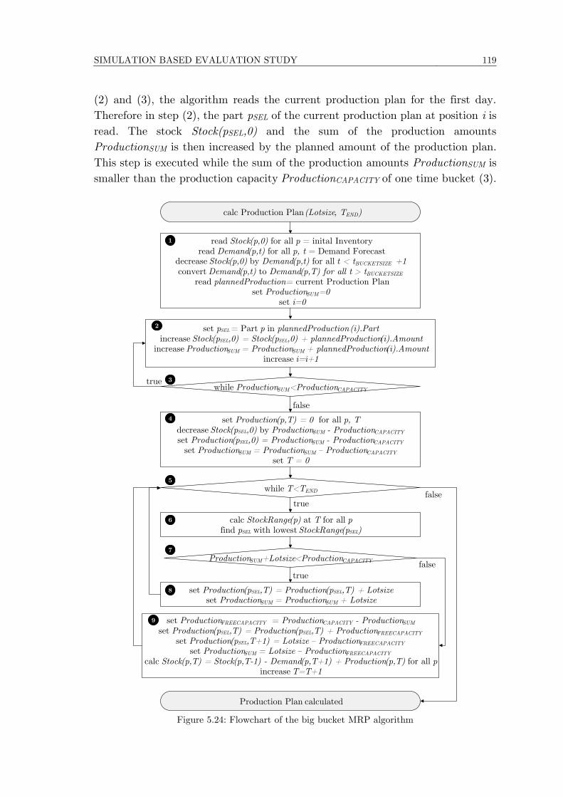
SIMULATION BASED EVALUATION STUDY 119
(2) and (3), the algorithm reads the current production plan for the first day.
Therefore in step (2), the part pSEL of the current production plan at position i is
read. The stock Stock(pSEL,0) and the sum of the production amounts
ProductionSUM is then increased by the planned amount of the production plan.
This step is executed while the sum of the production amounts ProductionSUM is
smaller than the production capacity ProductionCAPACITY of one time bucket (3).
Figure 5.24: Flowchart of the big bucket MRP algorithm
calc Production Plan(Lotsize, TEND)
read Stock(p,0) for all p = inital Inventory read Demand(p,t) for all p, t = Demand Forecast
decrease Stock(p,0) by Demand(p,t) for all t < tBUCKETSIZE +1convert Demand(p,t) to Demand(p,T) for all t > tBUCKETSIZE
read plannedProduction= current Production Planset ProductionSUM=0
set i=0
1
while ProductionSUM<ProductionCAPACITY
set pSEL = Part p in plannedProduction (i).Partincrease Stock(pSEL,0) = Stock(pSEL,0) + plannedProduction(i).Amount
increase ProductionSUM = ProductionSUM + plannedProduction(i).Amountincrease i=i+1
true
set Production(p,T) = 0 for all p, Tdecrease Stock(pSEL,0) by ProductionSUM - ProductionCAPACITY
set Production(pSEL,0) = ProductionSUM - ProductionCAPACITY
set ProductionSUM = ProductionSUM – ProductionCAPACITY
set T = 0
while T<TEND
calc StockRange(p) at T for all pfind pSEL with lowest StockRange(pSEL)
ProductionSUM+Lotsize<ProductionCAPACITY
set Production(pSEL,T) = Production(pSEL,T) + Lotsizeset ProductionSUM = ProductionSUM + Lotsize
set ProductionFREECAPACITY = ProductionCAPACITY - ProductionSUM
set Production(pSEL,T) = Production(pSEL,T) + ProductionFREECAPACITY
set Production(pSEL,T+1) = Lotsize – ProductionFREECAPACITY
set ProductionSUM = Lotsize – ProductionFREECAPACITY
calc Stock(p,T) = Stock(p,T-1) - Demand(p,T+1) + Production(p,T) for all pincrease T=T+1
false
true
true
false
false
Production Plan calculated
2
3
4
5
6
7
8
9
SIMULATION BASED EVALUATION STUDY 120
Next in step (4), the production amounts Production(p,T) for all parts p and time
steps T are set to zero. The stock of the part pSEL at position T=0 is then
decreased by the over production calculated by the capacity minus the sum of
the production amounts and the production of the part pSEL at position T=0. The
sum of the production amounts is also set to this value. Last in step (4), the time
step index T is set to zero. In step (5), a loop of the following steps (6) to (9) is
performed in which lots in the defined size Lotsize are added to the individual
time steps. Therefore in step (6), the algorithm searches for a part pSEL with the
lowest inventory range StockRange(pSEL). In case that the sum of the production
amounts plus the lot size is smaller than the production capacity, the lot can be
directly added to the actual time step and the sum of the production amounts is
increased by the lot size (8). Otherwise (9) the free capacity is calculated and the
to be added lot is split by this amount between the actual time step T and the
next time step T+1. Thereby, the new stock is calculated and the time step index
T is increased by one (9).
This algorithm has obviously the limitation that the lot size cannot be bigger
than the capacity of two big bucket time steps. Furthermore, it is assumed that
the lead time is not longer than 24 hours.
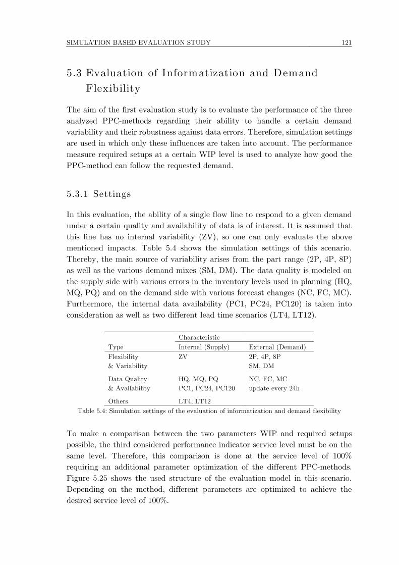
SIMULATION BASED EVALUATION STUDY 121
5.3 Evaluation of Informatization and Demand
Flexibility
The aim of the first evaluation study is to evaluate the performance of the three
analyzed PPC-methods regarding their ability to handle a certain demand
variability and their robustness against data errors. Therefore, simulation settings
are used in which only these influences are taken into account. The performance
measure required setups at a certain WIP level is used to analyze how good the
PPC-method can follow the requested demand.
5.3.1 Settings
In this evaluation, the ability of a single flow line to respond to a given demand
under a certain quality and availability of data is of interest. It is assumed that
this line has no internal variability (ZV), so one can only evaluate the above
mentioned impacts. Table 5.4 shows the simulation settings of this scenario.
Thereby, the main source of variability arises from the part range (2P, 4P, 8P)
as well as the various demand mixes (SM, DM). The data quality is modeled on
the supply side with various errors in the inventory levels used in planning (HQ,
MQ, PQ) and on the demand side with various forecast changes (NC, FC, MC).
Furthermore, the internal data availability (PC1, PC24, PC120) is taken into
consideration as well as two different lead time scenarios (LT4, LT12).
Characteristic
Type Internal (Supply) External (Demand)
Flexibility
& Variability
ZV 2P, 4P, 8P
SM, DM
Data Quality
& Availability
HQ, MQ, PQ
PC1, PC24, PC120
NC, FC, MC
update every 24h
Others LT4, LT12
Table 5.4: Simulation settings of the evaluation of informatization and demand flexibility
To make a comparison between the two parameters WIP and required setups
possible, the third considered performance indicator service level must be on the
same level. Therefore, this comparison is done at the service level of 100%
requiring an additional parameter optimization of the different PPC-methods.
Figure 5.25 shows the used structure of the evaluation model in this scenario.
Depending on the method, different parameters are optimized to achieve the
desired service level of 100%.
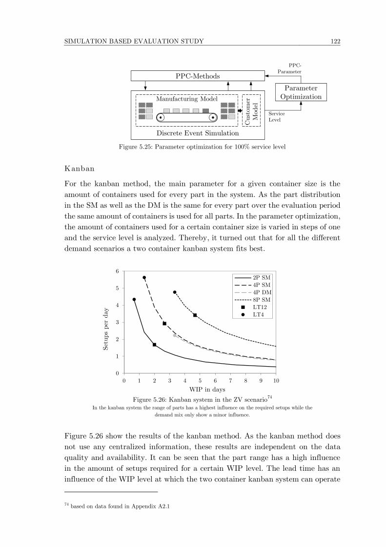
SIMULATION BASED EVALUATION STUDY 122
Figure 5.25: Parameter optimization for 100% service level
Kanban
For the kanban method, the main parameter for a given container size is the
amount of containers used for every part in the system. As the part distribution
in the SM as well as the DM is the same for every part over the evaluation period
the same amount of containers is used for all parts. In the parameter optimization,
the amount of containers used for a certain container size is varied in steps of one
and the service level is analyzed. Thereby, it turned out that for all the different
demand scenarios a two container kanban system fits best.
Figure 5.26: Kanban system in the ZV scenario
74
In the kanban system the range of parts has a highest influence on the required setups while the
demand mix only show a minor influence.
Figure 5.26 show the results of the kanban method. As the kanban method does
not use any centralized information, these results are independent on the data
quality and availability. It can be seen that the part range has a high influence
in the amount of setups required for a certain WIP level. The lead time has an
influence of the WIP level at which the two container kanban system can operate
74 based on data found in Appendix A2.1
ParameterOptimization
PPC-Parameter
ServiceLevel
Manufacturing Model
Discrete Event Simulation
Cust
omer
Mod
el
PPC-Methods
0
1
2
3
4
5
6
0 1 2 3 4 5 6 7 8 9 10
Set
ups
per
day
WIP in days
2P SM
4P SM
4P DM
8P SM
LT12
LT4
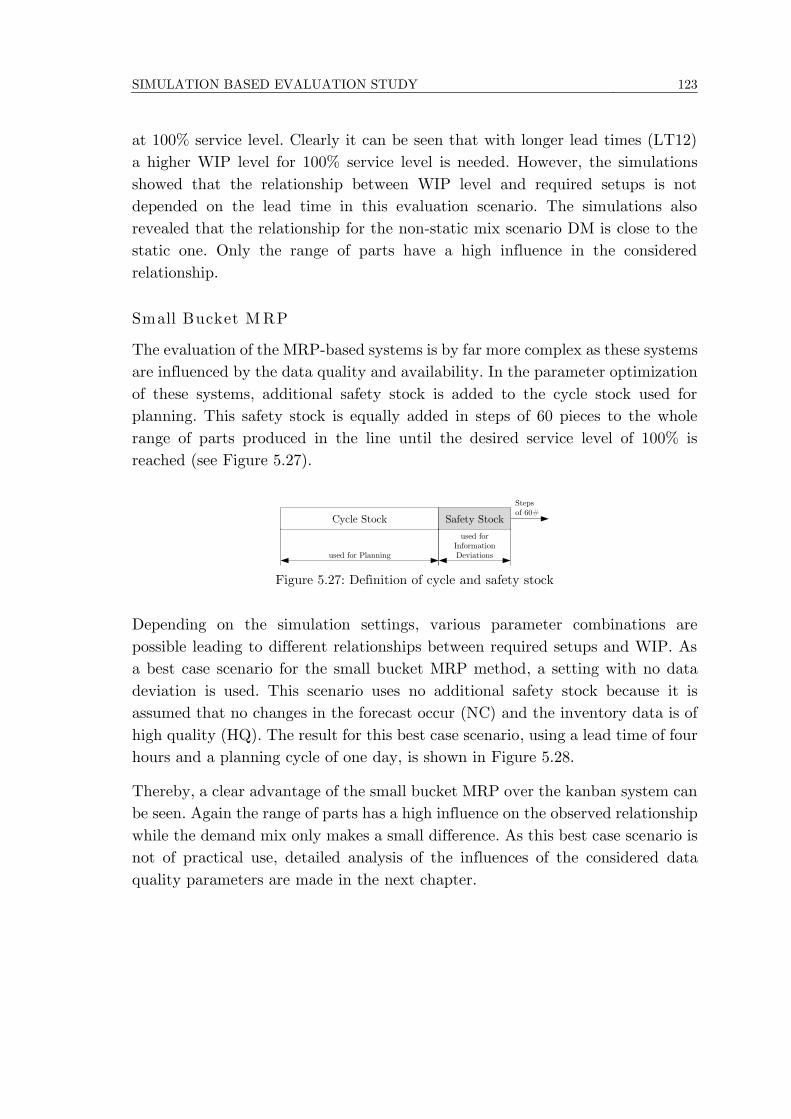
SIMULATION BASED EVALUATION STUDY 123
at 100% service level. Clearly it can be seen that with longer lead times (LT12)
a higher WIP level for 100% service level is needed. However, the simulations
showed that the relationship between WIP level and required setups is not
depended on the lead time in this evaluation scenario. The simulations also
revealed that the relationship for the non-static mix scenario DM is close to the
static one. Only the range of parts have a high influence in the considered
relationship.
Small Bucket M RP
The evaluation of the MRP-based systems is by far more complex as these systems
are influenced by the data quality and availability. In the parameter optimization
of these systems, additional safety stock is added to the cycle stock used for
planning. This safety stock is equally added in steps of 60 pieces to the whole
range of parts produced in the line until the desired service level of 100% is
reached (see Figure 5.27).
Figure 5.27: Definition of cycle and safety stock
Depending on the simulation settings, various parameter combinations are
possible leading to different relationships between required setups and WIP. As
a best case scenario for the small bucket MRP method, a setting with no data
deviation is used. This scenario uses no additional safety stock because it is
assumed that no changes in the forecast occur (NC) and the inventory data is of
high quality (HQ). The result for this best case scenario, using a lead time of four
hours and a planning cycle of one day, is shown in Figure 5.28.
Thereby, a clear advantage of the small bucket MRP over the kanban system can
be seen. Again the range of parts has a high influence on the observed relationship
while the demand mix only makes a small difference. As this best case scenario is
not of practical use, detailed analysis of the influences of the considered data
quality parameters are made in the next chapter.
Cycle Stock Safety Stock
Stepsof 60#
used for Planning
used for Information Deviations
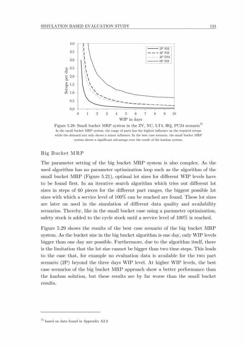
SIMULATION BASED EVALUATION STUDY 124
Figure 5.28: Small bucket MRP system in the ZV, NC, LT4, HQ, PC24 scenario
75
In the small bucket MRP system, the range of parts has the highest influence on the required setups
while the demand mix only shows a minor influence. In the best case scenario, the small bucket MRP
system shows a significant advantage over the result of the kanban system.
Big Bucket M RP
The parameter setting of the big bucket MRP system is also complex. As the
used algorithm has no parameter optimization loop such as the algorithm of the
small bucket MRP (Figure 5.21), optimal lot sizes for different WIP levels have
to be found first. In an iterative search algorithm which tries out different lot
sizes in steps of 60 pieces for the different part ranges, the biggest possible lot
sizes with which a service level of 100% can be reached are found. These lot sizes
are later on used in the simulation of different data quality and availability
scenarios. Thereby, like in the small bucket case using a parameter optimization,
safety stock is added to the cycle stock until a service level of 100% is reached.
Figure 5.29 shows the results of the best case scenario of the big bucket MRP
system. As the bucket size in the big bucket algorithm is one day, only WIP levels
bigger than one day are possible. Furthermore, due to the algorithm itself, there
is the limitation that the lot size cannot be bigger than two time steps. This leads
to the case that, for example no evaluation data is available for the two part
scenario (2P) beyond the three days WIP level. At higher WIP levels, the best
case scenarios of the big bucket MRP approach show a better performance than
the kanban solution, but these results are by far worse than the small bucket
results.
75 based on data found in Appendix A2.2
0,0
0,5
1,0
1,5
2,0
2,5
3,0
3,5
4,0
0 1 2 3 4 5 6 7 8 9 10
Set
ups
per
day
WIP in days
2P SM
4P SM
4P DM
8P SM
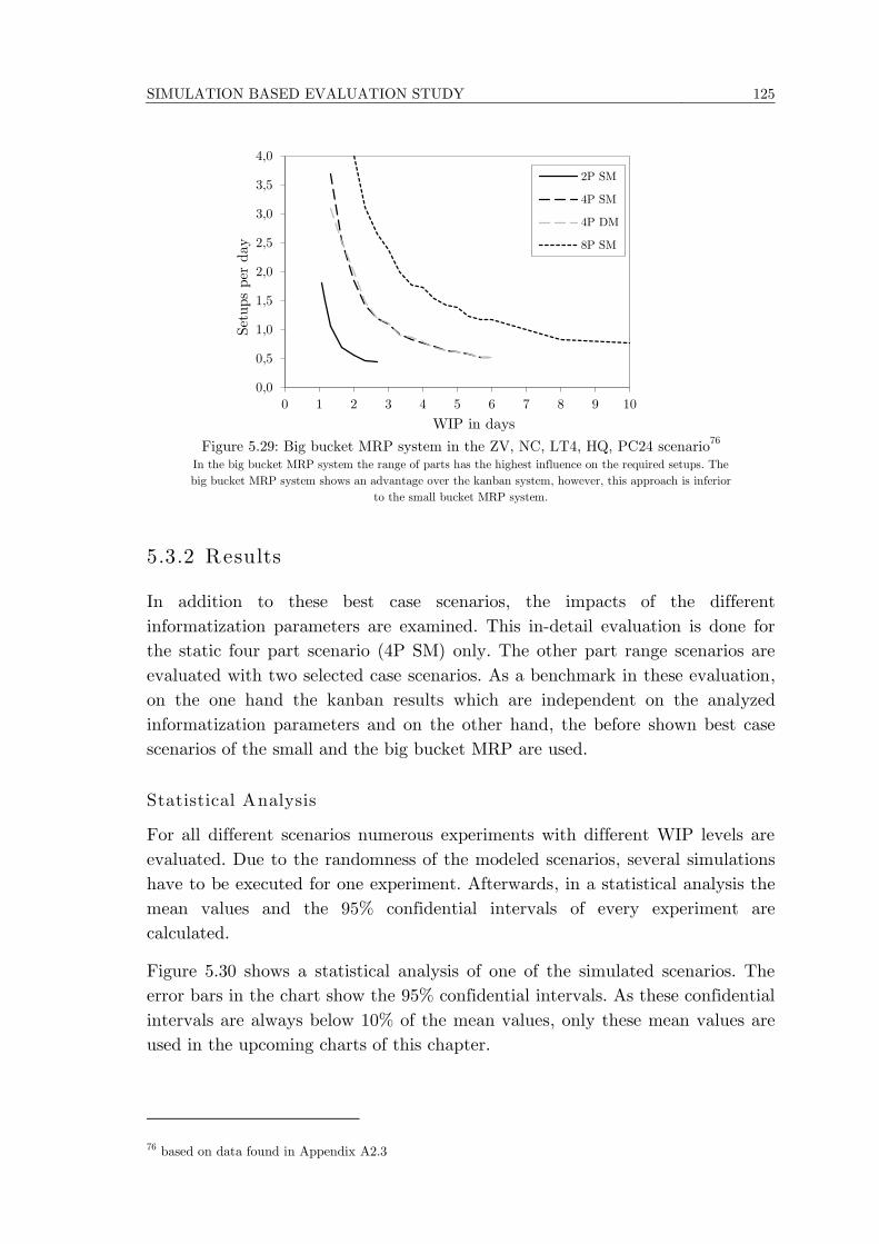
SIMULATION BASED EVALUATION STUDY 125
Figure 5.29: Big bucket MRP system in the ZV, NC, LT4, HQ, PC24 scenario
76
In the big bucket MRP system the range of parts has the highest influence on the required setups. The
big bucket MRP system shows an advantage over the kanban system, however, this approach is inferior
to the small bucket MRP system.
5.3.2 Results
In addition to these best case scenarios, the impacts of the different
informatization parameters are examined. This in-detail evaluation is done for
the static four part scenario (4P SM) only. The other part range scenarios are
evaluated with two selected case scenarios. As a benchmark in these evaluation,
on the one hand the kanban results which are independent on the analyzed
informatization parameters and on the other hand, the before shown best case
scenarios of the small and the big bucket MRP are used.
Statistical Analysis
For all different scenarios numerous experiments with different WIP levels are
evaluated. Due to the randomness of the modeled scenarios, several simulations
have to be executed for one experiment. Afterwards, in a statistical analysis the
mean values and the 95% confidential intervals of every experiment are
calculated.
Figure 5.30 shows a statistical analysis of one of the simulated scenarios. The
error bars in the chart show the 95% confidential intervals. As these confidential
intervals are always below 10% of the mean values, only these mean values are
used in the upcoming charts of this chapter.
76 based on data found in Appendix A2.3
0,0
0,5
1,0
1,5
2,0
2,5
3,0
3,5
4,0
0 1 2 3 4 5 6 7 8 9 10
Set
ups
per
day
WIP in days
2P SM
4P SM
4P DM
8P SM
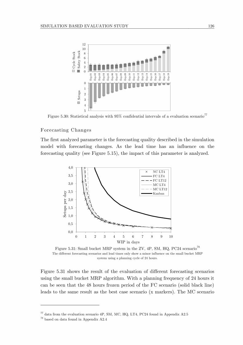
SIMULATION BASED EVALUATION STUDY 126
Figure 5.30: Statistical analysis with 95% confidential intervals of a evaluation scenario
77
Forecasting Changes
The first analyzed parameter is the forecasting quality described in the simulation
model with forecasting changes. As the lead time has an influence on the
forecasting quality (see Figure 5.15), the impact of this parameter is analyzed.
Figure 5.31: Small bucket MRP system in the ZV, 4P, SM, HQ, PC24 scenario
78
The different forecasting scenarios and lead times only show a minor influence on the small bucket MRP
system using a planning cycle of 24 hours.
Figure 5.31 shows the result of the evaluation of different forecasting scenarios
using the small bucket MRP algorithm. With a planning frequency of 24 hours it
can be seen that the 48 hours frozen period of the FC scenario (solid black line)
leads to the same result as the best case scenario (x markers). The MC scenario
77 data from the evaluation scenario 4P, SM, MC, HQ, LT4, PC24 found in Appendix A2.5 78 based on data found in Appendix A2.4
0
2
4
6
8
10
12
Exp.0
1
Exp.0
2
Exp.0
3
Exp.0
4
Exp.0
5
Exp.0
6
Exp.0
7
Exp.0
8
Exp.0
9
Exp.1
0
Exp.1
1
Exp.1
2
Exp.1
3
Exp.1
4
Exp.1
5
Exp.1
6
Exp.1
7
Exp.1
8
Exp.1
9
0
1
2
3
4
5
Cycl
e Sto
ck
Saf
ety S
tock
Set
ups
0,0
0,5
1,0
1,5
2,0
2,5
3,0
3,5
4,0
0 1 2 3 4 5 6 7 8 9 10
Set
ups
per
day
WIP in days
NC LT4
FC LT4
FC LT12
MC LT4
MC LT12
Kanban
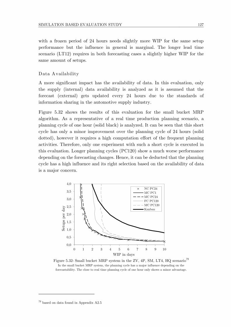
SIMULATION BASED EVALUATION STUDY 127
with a frozen period of 24 hours needs slightly more WIP for the same setup
performance but the influence in general is marginal. The longer lead time
scenario (LT12) requires in both forecasting cases a slightly higher WIP for the
same amount of setups.
Data Availability
A more significant impact has the availability of data. In this evaluation, only
the supply (internal) data availability is analyzed as it is assumed that the
forecast (external) gets updated every 24 hours due to the standards of
information sharing in the automotive supply industry.
Figure 5.32 shows the results of this evaluation for the small bucket MRP
algorithm. As a representative of a real time production planning scenario, a
planning cycle of one hour (solid black) is analyzed. It can be seen that this short
cycle has only a minor improvement over the planning cycle of 24 hours (solid
dotted), however it requires a high computation effort of the frequent planning
activities. Therefore, only one experiment with such a short cycle is executed in
this evaluation. Longer planning cycles (PC120) show a much worse performance
depending on the forecasting changes. Hence, it can be deducted that the planning
cycle has a high influence and its right selection based on the availability of data
is a major concern.
Figure 5.32: Small bucket MRP system in the ZV, 4P, SM, LT4, HQ scenario
79
In the small bucket MRP system, the planning cycle has a major influence depending on the
forecastability. The close to real time planning cycle of one hour only shows a minor advantage.
79 based on data found in Appendix A2.5
0,0
0,5
1,0
1,5
2,0
2,5
3,0
3,5
4,0
0 1 2 3 4 5 6 7 8 9 10
Set
ups
per
day
WIP in days
NC PC24
MC PC1
MC PC24
FC PC120
MC PC120
Kanban
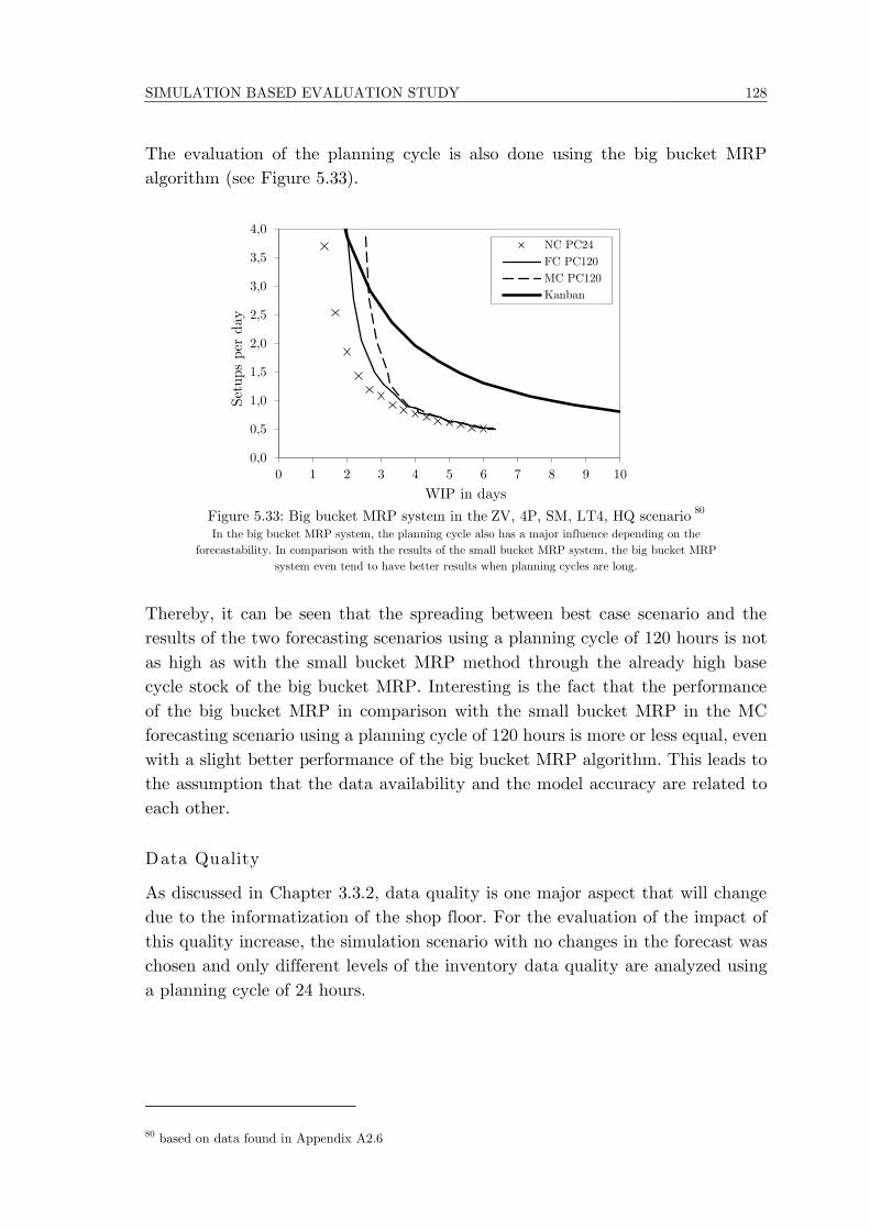
SIMULATION BASED EVALUATION STUDY 128
The evaluation of the planning cycle is also done using the big bucket MRP
algorithm (see Figure 5.33).
Figure 5.33: Big bucket MRP system in the
ZV, 4P, SM, LT4, HQ scenario
80
In the big bucket MRP system, the planning cycle also has a major influence depending on the
forecastability. In comparison with the results of the small bucket MRP system, the big bucket MRP
system even tend to have better results when planning cycles are long.
Thereby, it can be seen that the spreading between best case scenario and the
results of the two forecasting scenarios using a planning cycle of 120 hours is not
as high as with the small bucket MRP method through the already high base
cycle stock of the big bucket MRP. Interesting is the fact that the performance
of the big bucket MRP in comparison with the small bucket MRP in the MC
forecasting scenario using a planning cycle of 120 hours is more or less equal, even
with a slight better performance of the big bucket MRP algorithm. This leads to
the assumption that the data availability and the model accuracy are related to
each other.
Data Quality
As discussed in Chapter 3.3.2, data quality is one major aspect that will change
due to the informatization of the shop floor. For the evaluation of the impact of
this quality increase, the simulation scenario with no changes in the forecast was
chosen and only different levels of the inventory data quality are analyzed using
a planning cycle of 24 hours.
80 based on data found in Appendix A2.6
0,0
0,5
1,0
1,5
2,0
2,5
3,0
3,5
4,0
0 1 2 3 4 5 6 7 8 9 10
Set
ups
per
day
WIP in days
NC PC24
FC PC120
MC PC120
Kanban
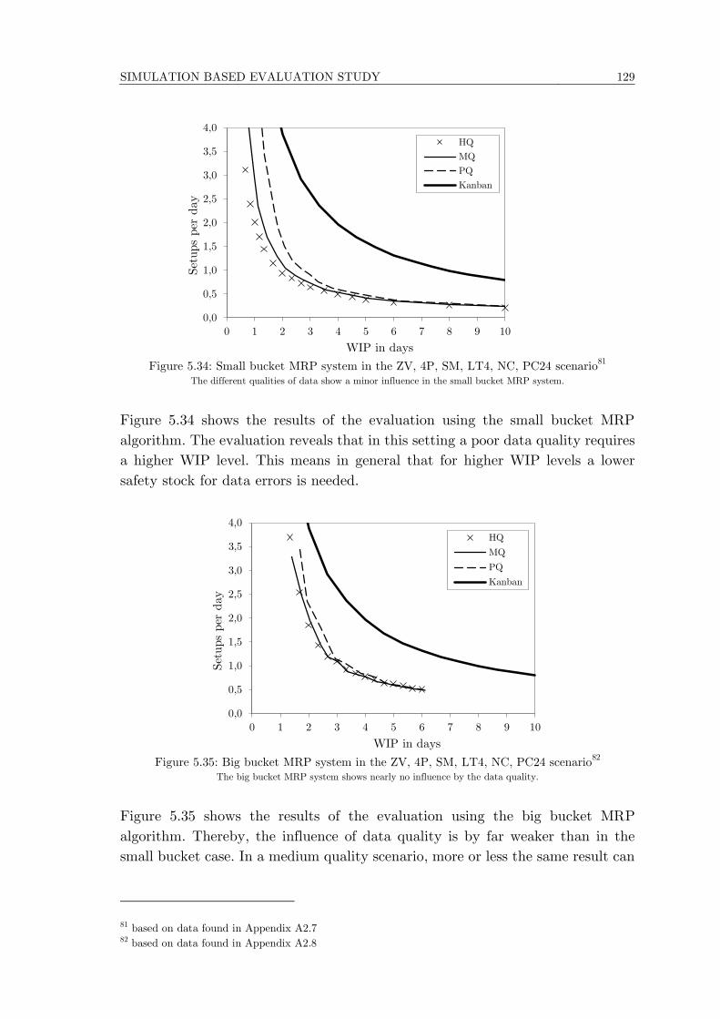
SIMULATION BASED EVALUATION STUDY 129
Figure 5.34: Small bucket MRP system in the ZV, 4P, SM, LT4, NC, PC24 scenario
81
The different qualities of data show a minor influence in the small bucket MRP system.
Figure 5.34 shows the results of the evaluation using the small bucket MRP
algorithm. The evaluation reveals that in this setting a poor data quality requires
a higher WIP level. This means in general that for higher WIP levels a lower
safety stock for data errors is needed.
Figure 5.35: Big bucket MRP system in the ZV, 4P, SM, LT4, NC, PC24 scenario
82
The big bucket MRP system shows nearly no influence by the data quality.
Figure 5.35 shows the results of the evaluation using the big bucket MRP
algorithm. Thereby, the influence of data quality is by far weaker than in the
small bucket case. In a medium quality scenario, more or less the same result can
81 based on data found in Appendix A2.7 82 based on data found in Appendix A2.8
0,0
0,5
1,0
1,5
2,0
2,5
3,0
3,5
4,0
0 1 2 3 4 5 6 7 8 9 10
Set
ups
per
day
WIP in days
HQ
MQ
PQ
Kanban
0,0
0,5
1,0
1,5
2,0
2,5
3,0
3,5
4,0
0 1 2 3 4 5 6 7 8 9 10
Set
ups
per
day
WIP in days
HQ
MQ
PQ
Kanban
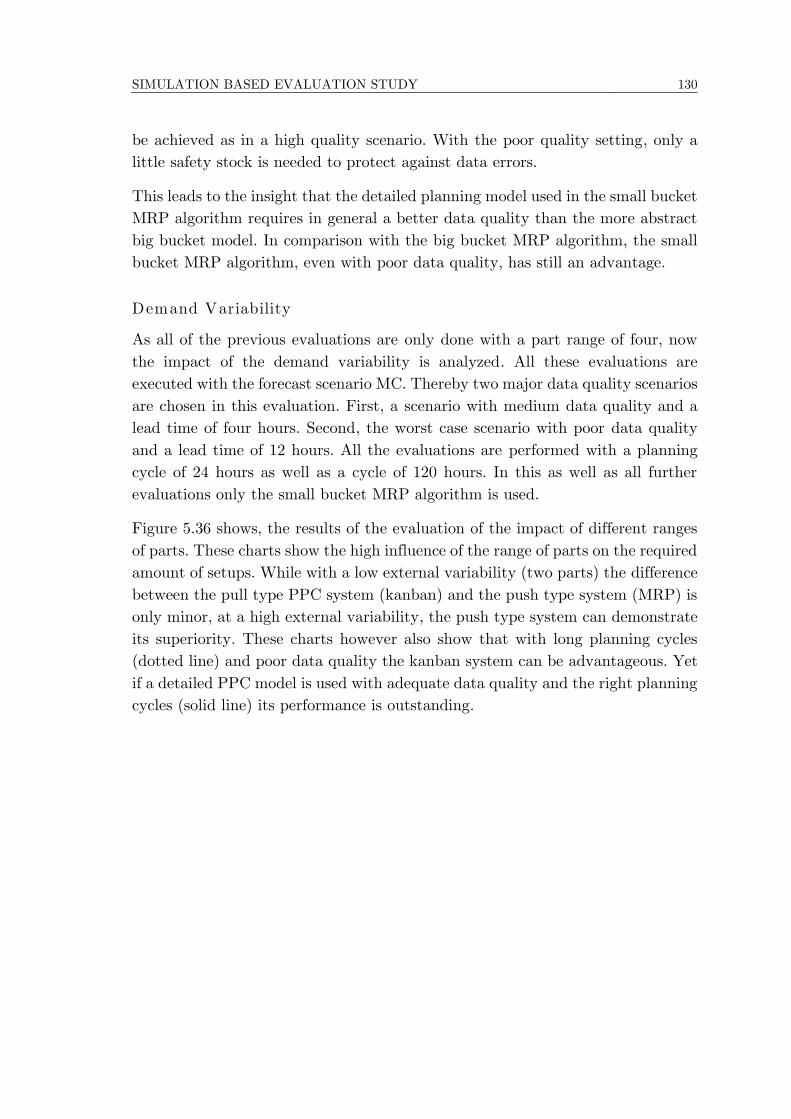
SIMULATION BASED EVALUATION STUDY 130
be achieved as in a high quality scenario. With the poor quality setting, only a
little safety stock is needed to protect against data errors.
This leads to the insight that the detailed planning model used in the small bucket
MRP algorithm requires in general a better data quality than the more abstract
big bucket model. In comparison with the big bucket MRP algorithm, the small
bucket MRP algorithm, even with poor data quality, has still an advantage.
Demand Variability
As all of the previous evaluations are only done with a part range of four, now
the impact of the demand variability is analyzed. All these evaluations are
executed with the forecast scenario MC. Thereby two major data quality scenarios
are chosen in this evaluation. First, a scenario with medium data quality and a
lead time of four hours. Second, the worst case scenario with poor data quality
and a lead time of 12 hours. All the evaluations are performed with a planning
cycle of 24 hours as well as a cycle of 120 hours. In this as well as all further
evaluations only the small bucket MRP algorithm is used.
Figure 5.36 shows, the results of the evaluation of the impact of different ranges
of parts. These charts show the high influence of the range of parts on the required
amount of setups. While with a low external variability (two parts) the difference
between the pull type PPC system (kanban) and the push type system (MRP) is
only minor, at a high external variability, the push type system can demonstrate
its superiority. These charts however also show that with long planning cycles
(dotted line) and poor data quality the kanban system can be advantageous. Yet
if a detailed PPC model is used with adequate data quality and the right planning
cycles (solid line) its performance is outstanding.
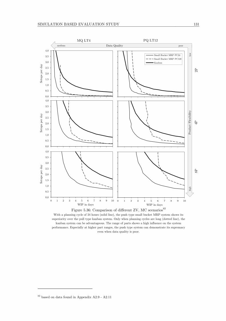
SIMULATION BASED EVALUATION STUDY 131
Figure 5.36: Comparison of different ZV, MC scenarios
83
With a planning cycle of 24 hours (solid line), the push type small bucket MRP system shows its
superiority over the pull type kanban system. Only when planning cycles are long (dotted line), the
kanban system can be advantageous. The range of parts shows a high influence on the system
performance. Especially at higher part ranges, the push type system can demonstrate its supremacy
even when data quality is poor.
83 based on data found in Appendix A2.9 - A2.11
0,0
0,5
1,0
1,5
2,0
2,5
3,0
3,5
4,0
0 1 2 3 4 5 6 7 8 9 10
Set
ups
per
day
WIP in days
Small Bucket MRP PC24
Small Bucket MRP PC120
Kanban
0,0
0,5
1,0
1,5
2,0
2,5
3,0
3,5
4,0
0 1 2 3 4 5 6 7 8 9 10
Set
ups
per
day
WIP in days
0,0
0,5
1,0
1,5
2,0
2,5
3,0
3,5
4,0
0 1 2 3 4 5 6 7 8 9 10
Set
ups
per
day
WIP in days
2P4P
8P
0,0
0,5
1,0
1,5
2,0
2,5
3,0
3,5
4,0
0 1 2 3 4 5 6 7 8 9 10
WIP in days
0,0
0,5
1,0
1,5
2,0
2,5
3,0
3,5
4,0
0 1 2 3 4 5 6 7 8 9 10
WIP in days
0,0
0,5
1,0
1,5
2,0
2,5
3,0
3,5
4,0
0 1 2 3 4 5 6 7 8 9 10
WIP in days
PQ LT12MQ LT4
Data Quality
Pro
duct
Fle
xib
ility
medium poor
low
hig
h
Set
ups
per
day
Set
ups
per
day
Set
ups
per
day
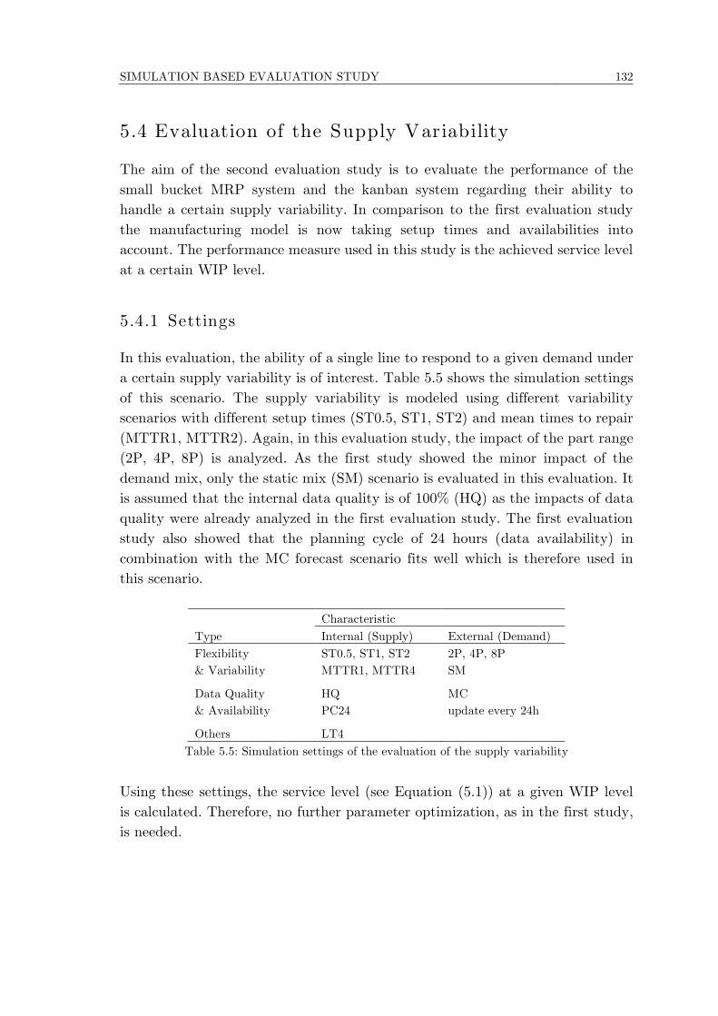
SIMULATION BASED EVALUATION STUDY 132
5.4 Evaluation of the Supply Variability
The aim of the second evaluation study is to evaluate the performance of the
small bucket MRP system and the kanban system regarding their ability to
handle a certain supply variability. In comparison to the first evaluation study
the manufacturing model is now taking setup times and availabilities into
account. The performance measure used in this study is the achieved service level
at a certain WIP level.
5.4.1 Settings
In this evaluation, the ability of a single line to respond to a given demand under
a certain supply variability is of interest. Table 5.5 shows the simulation settings
of this scenario. The supply variability is modeled using different variability
scenarios with different setup times (ST0.5, ST1, ST2) and mean times to repair
(MTTR1, MTTR2). Again, in this evaluation study, the impact of the part range
(2P, 4P, 8P) is analyzed. As the first study showed the minor impact of the
demand mix, only the static mix (SM) scenario is evaluated in this evaluation. It
is assumed that the internal data quality is of 100% (HQ) as the impacts of data
quality were already analyzed in the first evaluation study. The first evaluation
study also showed that the planning cycle of 24 hours (data availability) in
combination with the MC forecast scenario fits well which is therefore used in
this scenario.
Characteristic
Type Internal (Supply) External (Demand)
Flexibility
& Variability
ST0.5, ST1, ST2
MTTR1, MTTR4
2P, 4P, 8P
SM
Data Quality
& Availability
HQ
PC24
MC
update every 24h
Others LT4
Table 5.5: Simulation settings of the evaluation of the supply variability
Using these settings, the service level (see Equation (5.1)) at a given WIP level
is calculated. Therefore, no further parameter optimization, as in the first study,
is needed.
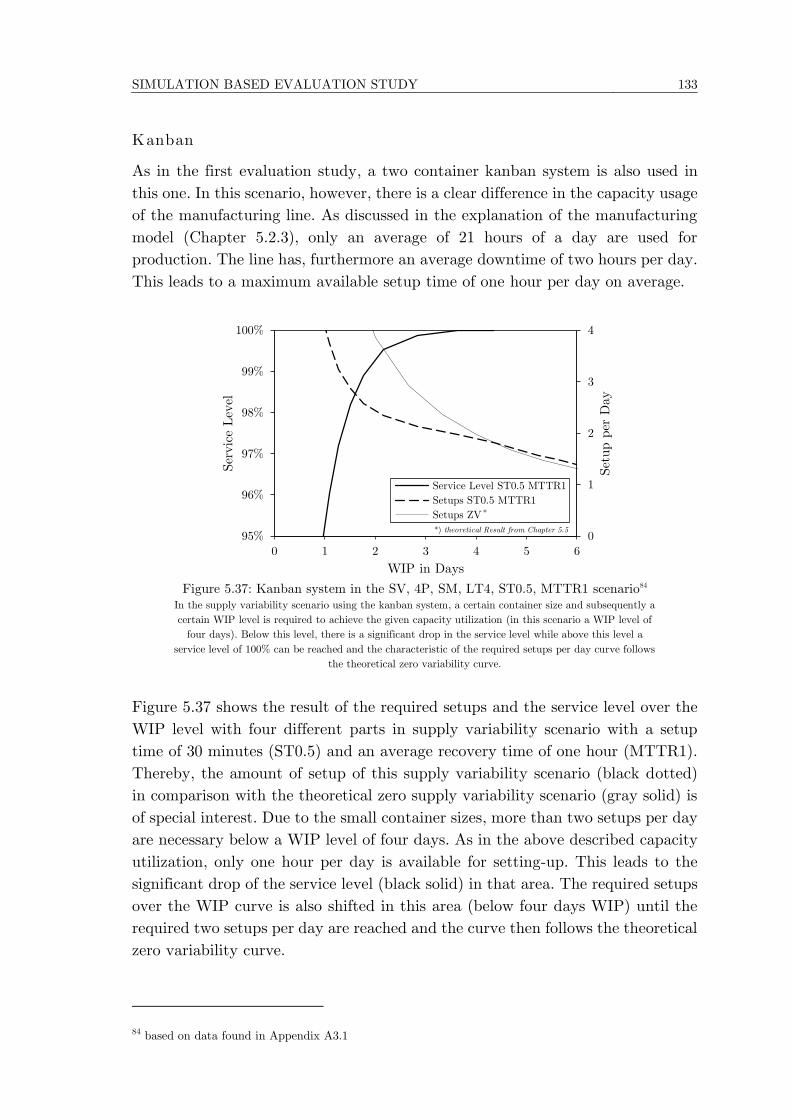
SIMULATION BASED EVALUATION STUDY 133
Kanban
As in the first evaluation study, a two container kanban system is also used in
this one. In this scenario, however, there is a clear difference in the capacity usage
of the manufacturing line. As discussed in the explanation of the manufacturing
model (Chapter 5.2.3), only an average of 21 hours of a day are used for
production. The line has, furthermore an average downtime of two hours per day.
This leads to a maximum available setup time of one hour per day on average.
Figure 5.37: Kanban system in the SV, 4P, SM, LT4, ST0.5, MTTR1 scenario84
In the supply variability scenario using the kanban system, a certain container size and subsequently a
certain WIP level is required to achieve the given capacity utilization (in this scenario a WIP level of
four days). Below this level, there is a significant drop in the service level while above this level a
service level of 100% can be reached and the characteristic of the required setups per day curve follows
the theoretical zero variability curve.
Figure 5.37 shows the result of the required setups and the service level over the
WIP level with four different parts in supply variability scenario with a setup
time of 30 minutes (ST0.5) and an average recovery time of one hour (MTTR1).
Thereby, the amount of setup of this supply variability scenario (black dotted)
in comparison with the theoretical zero supply variability scenario (gray solid) is
of special interest. Due to the small container sizes, more than two setups per day
are necessary below a WIP level of four days. As in the above described capacity
utilization, only one hour per day is available for setting-up. This leads to the
significant drop of the service level (black solid) in that area. The required setups
over the WIP curve is also shifted in this area (below four days WIP) until the
required two setups per day are reached and the curve then follows the theoretical
zero variability curve.
84 based on data found in Appendix A3.1
0
1
2
3
4
95%
96%
97%
98%
99%
100%
0 1 2 3 4 5 6
Set
up p
er D
ay
Ser
vic
e Lev
el
WIP in Days
Service Level ST0.5 MTTR1
Setups ST0.5 MTTR1
Setups ZV
*) theoretical Result from Chapter 5.5
*
SIMULATION BASED EVALUATION STUDY 134
The utilization chart of Figure 5.38 for the individual simulation results show an
equal result with the idle ratio. After a WIP level of four days (EXP08) is reached,
the number of setups is low enough to enable an idle time at the manufacturing
line. In all previous experiments (EXP01-EXP07) the setups proportion is higher
than the available capacity for setting-up leading to a decline in the working
proportion with the consequent drop in the service level.
Figure 5.38 Utilization of the kanban system in the SV, 4P, SM, LT4, ST0.5, MTTR1 scenario85
In the EXP01-EXP07, the proportion for setting-up is higher than the reserved capacity for setting-up
leading to a drop in the working proportion and consequently a decrease of the service level.
Small Bucket M RP
For the small bucket MRP system, in addition to the basic algorithm (see Figure
5.21) a WIP control is needed in this supply variability scenario. The MRP-based
algorithm has to be enhanced in a way that only the amount of hours needed to
reach the desired WIP level are used for production.
Figure 5.39 shows the used algorithm for the WIP control which includes a safety
stock underride functionality in case of under capacity. This algorithm is used in
addition to the already explained small bucket MRP algorithm (see Figure 5.19)
and its parameter optimization algorithm (see Figure 5.21).
In the first step (1) of this algorithm, the current available operational inventory
(minus the safety inventory) is read and stored in the variable StockTOTAL. The
desired total inventory level StockTARGET and the individual safety inventories for
every part p StockSAFETY(p) is also read. In the last action of the first step, the
difference between the inventory target StockTARGET and the actual inventory
StockTOTAL divided by the capacity of one day is calculated, rounded up and
stored in the variable tDIFFERENCE. This value indicated how many hours the
actual inventory is below (positive tDIFFERENCE) or above (negative tDIFFERENCE)
85 based on data found in Appendix A3.1
80%
85%
90%
95%
100%
EX
P01
EX
P02
EX
P03
EX
P04
EX
P05
EX
P06
EX
P07
EX
P08
EX
P09
EX
P10
EX
P11
EX
P12
EX
P13
Failed
Idle
Setting-up
Working
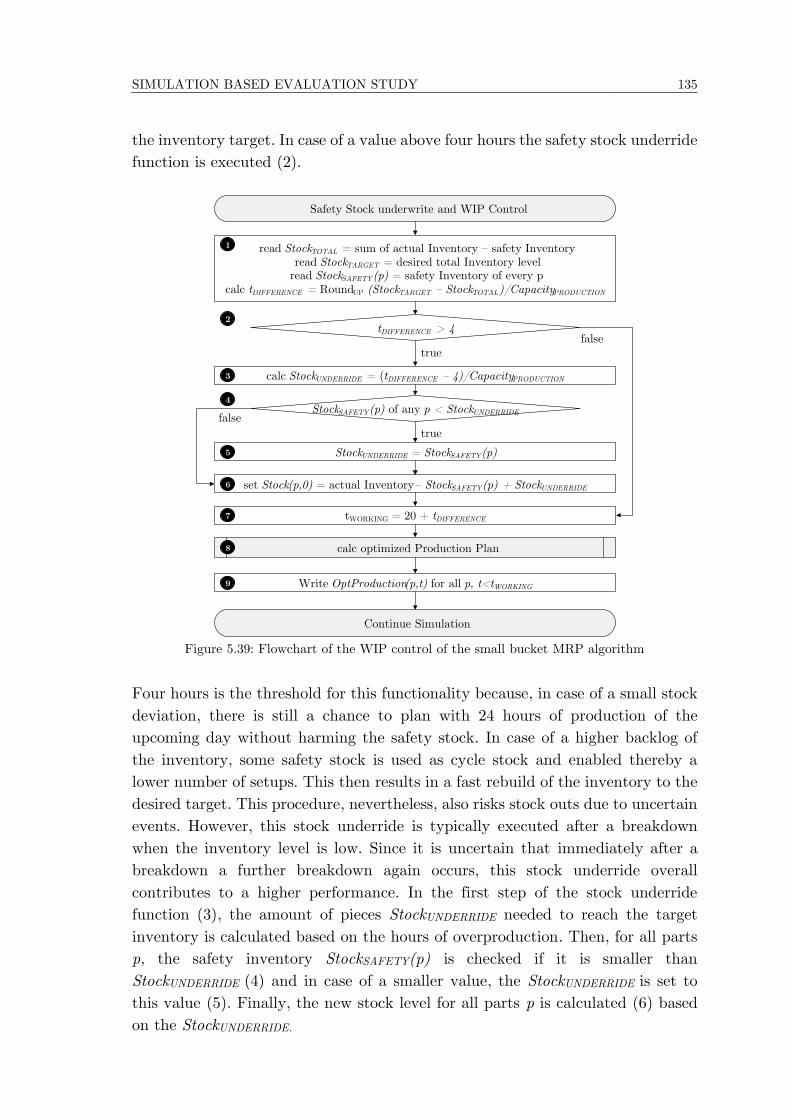
SIMULATION BASED EVALUATION STUDY 135
the inventory target. In case of a value above four hours the safety stock underride
function is executed (2).
Figure 5.39: Flowchart of the WIP control of the small bucket MRP algorithm
Four hours is the threshold for this functionality because, in case of a small stock
deviation, there is still a chance to plan with 24 hours of production of the
upcoming day without harming the safety stock. In case of a higher backlog of
the inventory, some safety stock is used as cycle stock and enabled thereby a
lower number of setups. This then results in a fast rebuild of the inventory to the
desired target. This procedure, nevertheless, also risks stock outs due to uncertain
events. However, this stock underride is typically executed after a breakdown
when the inventory level is low. Since it is uncertain that immediately after a
breakdown a further breakdown again occurs, this stock underride overall
contributes to a higher performance. In the first step of the stock underride
function (3), the amount of pieces StockUNDERRIDE needed to reach the target
inventory is calculated based on the hours of overproduction. Then, for all parts
p, the safety inventory StockSAFETY(p) is checked if it is smaller than
StockUNDERRIDE (4) and in case of a smaller value, the StockUNDERRIDE is set to
this value (5). Finally, the new stock level for all parts p is calculated (6) based
on the StockUNDERRIDE.
Safety Stock underwrite and WIP Control
read StockTOTAL = sum of actual Inventory – safety Inventoryread StockTARGET = desired total Inventory level
read StockSAFETY(p) = safety Inventory of every pcalc tDIFFERENCE = RoundUP (StockTARGET – StockTOTAL)/CapacityPRODUCTION
tDIFFERENCE > 4
calc StockUNDERRIDE = (tDIFFERENCE – 4)/CapacityPRODUCTION
StockSAFETY(p) of any p < StockUNDERRIDE
StockUNDERRIDE = StockSAFETY(p)
set Stock(p,0) = actual Inventory – StockSAFETY(p) + StockUNDERRIDE
true
true
tWORKING = 20 + tDIFFERENCE
false
calc optimized Production Plan
Write OptProduction(p,t) for all p, t<tWORKING
false
Continue Simulation
1
2
3
4
5
6
7
8
9
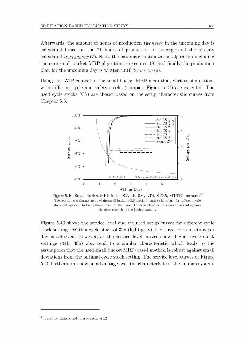
SIMULATION BASED EVALUATION STUDY 136
Afterwards, the amount of hours of production tWORKING in the upcoming day is
calculated based on the 21 hours of production on average and the already
calculated tDIFFERENCE (7). Next, the parameter optimization algorithm including
the core small bucket MRP algorithm is executed (8) and finally the production
plan for the upcoming day is written until tWORKING (9).
Using this WIP control in the small bucket MRP algorithm, various simulations
with different cycle and safety stocks (compare Figure 5.27) are executed. The
used cycle stocks (CS) are chosen based on the setup characteristic curves from
Chapter 5.3.
Figure 5.40: Small Bucket MRP in the SV, 4P, SM, LT4, ST0.5, MTTR1 scenario
86
The service level characteristic of the small bucket MRP method tends to be robust for different cycle
stock settings close to the optimum one. Furthermore, the service level curve shows an advantage over
the characteristic of the kanban system.
Figure 5.40 shows the service level and required setup curves for different cycle
stock settings. With a cycle stock of 32h (light gray), the target of two setups per
day is achieved. However, as the service level curves show, higher cycle stock
settings (34h, 36h) also tend to a similar characteristic which leads to the
assumption that the used small bucket MRP-based method is robust against small
deviations from the optimal cycle stock setting. The service level curves of Figure
5.40 furthermore show an advantage over the characteristic of the kanban system.
86 based on data found in Appendix A3.2
0
1
2
3
4
95%
96%
97%
98%
99%
100%
0 1 2 3 4 5 6Set
ups
per
Day
Ser
vic
e Lev
el
WIP in Days
32h CS34h CS36h CS32h CS34h CS36h CSSetups ZV
Ser
vic
e
Lev
el
CS...Cycle Stock *) theoretical Result from Chapter 5.5
Set
ups
*
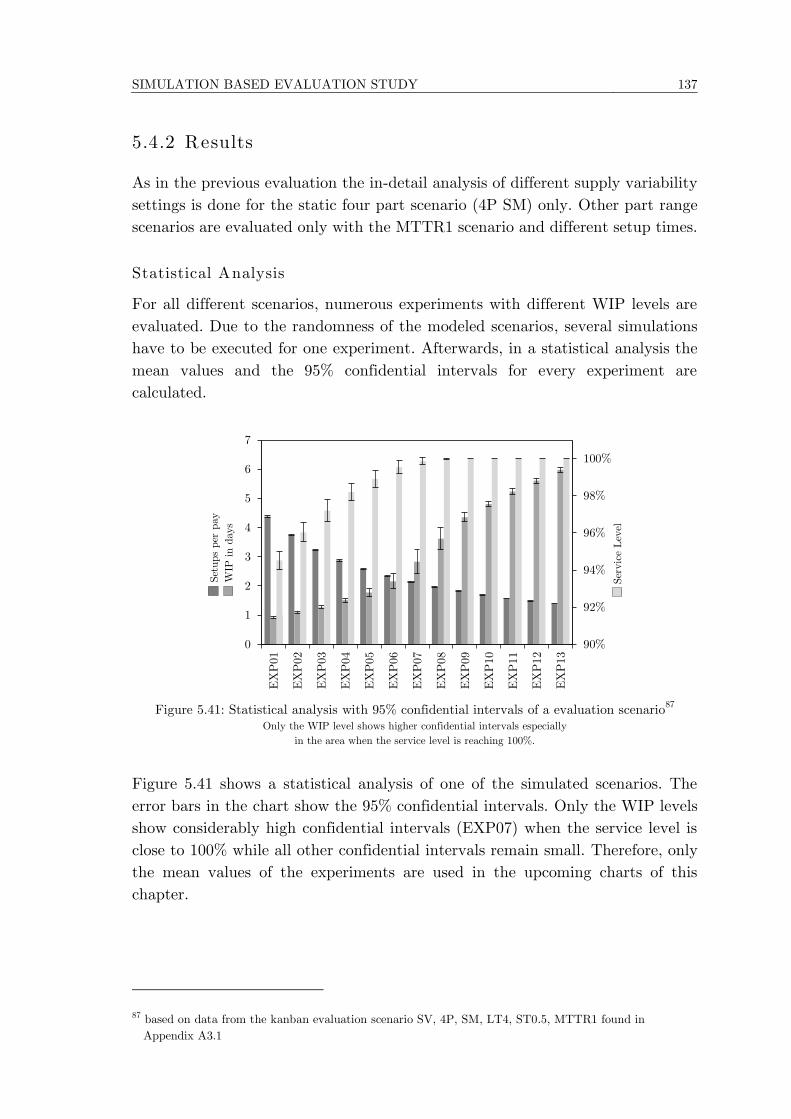
SIMULATION BASED EVALUATION STUDY 137
5.4.2 Results
As in the previous evaluation the in-detail analysis of different supply variability
settings is done for the static four part scenario (4P SM) only. Other part range
scenarios are evaluated only with the MTTR1 scenario and different setup times.
Statistical Analysis
For all different scenarios, numerous experiments with different WIP levels are
evaluated. Due to the randomness of the modeled scenarios, several simulations
have to be executed for one experiment. Afterwards, in a statistical analysis the
mean values and the 95% confidential intervals for every experiment are
calculated.
Figure 5.41: Statistical analysis with 95% confidential intervals of a evaluation scenario
87
Only the WIP level shows higher confidential intervals especially
in the area when the service level is reaching 100%.
Figure 5.41 shows a statistical analysis of one of the simulated scenarios. The
error bars in the chart show the 95% confidential intervals. Only the WIP levels
show considerably high confidential intervals (EXP07) when the service level is
close to 100% while all other confidential intervals remain small. Therefore, only
the mean values of the experiments are used in the upcoming charts of this
chapter.
87 based on data from the kanban evaluation scenario SV, 4P, SM, LT4, ST0.5, MTTR1 found in
Appendix A3.1
90%
92%
94%
96%
98%
100%
0
1
2
3
4
5
6
7
EX
P01
EX
P02
EX
P03
EX
P04
EX
P05
EX
P06
EX
P07
EX
P08
EX
P09
EX
P10
EX
P11
EX
P12
EX
P13
Set
ups
per
pay
WIP
in d
ays
Ser
vic
e Lev
el
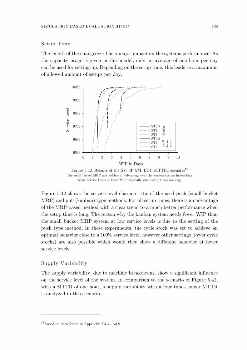
SIMULATION BASED EVALUATION STUDY 138
Setup Time
The length of the changeover has a major impact on the systems performance. As
the capacity usage is given in this model, only an average of one hour per day
can be used for setting-up. Depending on the setup time, this leads to a maximum
of allowed amount of setups per day.
Figure 5.42: Results of the SV, 4P SM, LT4, MTTR1 scenario
88
The small bucket MRP method has an advantage over the kanban system in reaching
better service levels at lower WIP especially when setup times are long.
Figure 5.42 shows the service level characteristic of the used push (small bucket
MRP) and pull (kanban) type methods. For all setup times, there is an advantage
of the MRP-based method with a clear trend to a much better performance when
the setup time is long. The reason why the kanban system needs fewer WIP than
the small bucket MRP system at low service levels is due to the setting of the
push type method. In these experiments, the cycle stock was set to achieve an
optimal behavior close to a 100% service level, however other settings (lower cycle
stocks) are also possible which would then show a different behavior at lower
service levels.
Supply Variability
The supply variability, due to machine breakdowns, show a significant influence
on the service level of the system. In comparison to the scenario of Figure 5.42,
with a MTTR of one hour, a supply variability with a four times longer MTTR
is analyzed in this scenario.
88 based on data found in Appendix A3.3 - A3.8
95%
96%
97%
98%
99%
100%
0 1 2 3 4 5 6 7 8 9 10
Ser
vic
e Lev
el
WIP in Days
ST0.5ST1ST2ST0.5ST1ST2
Kan
ban
Sm
all
Buck
et
MR
P
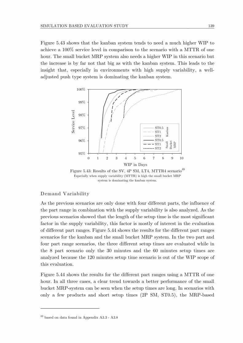
SIMULATION BASED EVALUATION STUDY 139
Figure 5.43 shows that the kanban system tends to need a much higher WIP to
achieve a 100% service level in comparison to the scenario with a MTTR of one
hour. The small bucket MRP system also needs a higher WIP in this scenario but
the increase is by far not that big as with the kanban system. This leads to the
insight that, especially in environments with high supply variability, a well-
adjusted push type system is dominating the kanban system.
Figure 5.43: Results of the SV, 4P SM, LT4, MTTR4 scenario
89
Especially when supply variability (MTTR) is high the small bucket MRP
system is dominating the kanban system.
Demand Variability
As the previous scenarios are only done with four different parts, the influence of
the part range in combination with the supply variability is also analyzed. As the
previous scenarios showed that the length of the setup time is the most significant
factor in the supply variability, this factor is mostly of interest in the evaluation
of different part ranges. Figure 5.44 shows the results for the different part ranges
scenarios for the kanban and the small bucket MRP system. In the two part and
four part range scenarios, the three different setup times are evaluated while in
the 8 part scenario only the 30 minutes and the 60 minutes setup times are
analyzed because the 120 minutes setup time scenario is out of the WIP scope of
this evaluation.
Figure 5.44 shows the results for the different part ranges using a MTTR of one
hour. In all three cases, a clear trend towards a better performance of the small
bucket MRP-system can be seen when the setup times are long. In scenarios with
only a few products and short setup times (2P SM, ST0.5), the MRP-based
89 based on data found in Appendix A3.3 - A3.8
95%
96%
97%
98%
99%
100%
0 1 2 3 4 5 6 7 8 9 10
Ser
vic
e Lev
el
WIP in Days
ST0.5
ST1
ST2
ST0.5
ST1
ST2
Kan
ban
Sm
all
Buck
et
MR
P
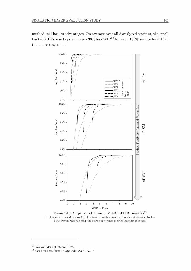
SIMULATION BASED EVALUATION STUDY 140
method still has its advantages. On average over all 8 analyzed settings, the small
bucket MRP-based system needs 36% less WIP90 to reach 100% service level than
the kanban system.
Figure 5.44: Comparison of different SV, MC, MTTR1 scenarios
91
In all analyzed scenarios, there is a clear trend towards a better performance of the small bucket
MRP-system when the setup times are long or when product flexibility is needed.
90 95% confidential interval ±8% 91 based on data found in Appendix A3.3 - A3.18
95%
96%
97%
98%
99%
100%Ser
vic
e Lev
el
WIP in Days
ST0.5ST1ST2ST0.5ST1ST2
2PSM
4PSM
8PSM
95%
96%
97%
98%
99%
100%
Ser
vic
e Lev
el
WIP in Days
95%
96%
97%
98%
99%
100%
0 1 2 3 4 5 6 7 8 9 10
Ser
vic
e Lev
el
WIP in Days
Pro
duct
Fle
xib
ility (
exte
rnal V
ari
ability)
Kan
ban
Sm
all
Buck
et
MR
P

Discussion
The greatest danger in times of turbulence is not
the turbulence; it is to act with yesterday’s logic. Peter Drucker (1909 - 2005)
Based on the results of the simulation based evaluation study of Chapter 5, this
chapter provides a complete overview on the found insights. Furthermore, these
insights are used to enhance an existing PPC configuration framework and a best
practice approach focusing on the overall total costs is suggested. Moreover, a use
case example of the configuration and implementation of a PPC system in the
automotive transmission production is given. Finally, the lessons learned from the
practical use case are discussed.
C H A P T E R
DISCUSSION 142
6.1 Insights
The research using the simulation based evaluation study showed to be a valued
approach in the understanding of the influencing factors in PPC. Furthermore,
the used required setups over WIP curves proved to be a simple and useful way
in the characterization of a PPC system. The gained insights in the evaluation
study of the PPC selection problem of disconnected flow lines are the following:
Solvability of PPC M odels
Even nowadays, the solvability of the easy to formulate but burdensome to solve
PPC LP models is still problematic. This is especially true when the problem size
is big due to a high number of different parts and a large number of planning
time steps. The used heuristics in this evaluation study showed to be a good
alternative. Thereby, especially the use of the inventory ranges turned out to be
a powerful and simple formulation that can be solved close to optimality in just
a few milliseconds.
PPC M odel Accuracy
Models are always only a limited representation of reality. In the process of model
building delimitation, reduction, decomposition, aggregation and abstraction are
used to capture the major elements and influencing factors of the complex reality.
Several different PPC models with different accuracies regarding their
representation of time, the used mechanisms for lot sizing, the capacity
consideration etc. exist. In the evaluation study, two contrary PPC models with
different modeling approaches for the planning time where analyzed. The
simulations showed that data availability and PPC modeling accuracy are related
to each other. The simple and abstract big bucket time model showed a slightly
better performance when data availability was bad. On the contrary, only the
more detailed small bucket time model could use the advantages of high data
availability. This phenomenon can be explained using the law of requisite variety
of Ashby (1956). For the investigated focus area, it can be deducted that the
model complexity of the control system (PPC model accuracy) is corresponding
to the through data known complexity (data availability) of the controlled
manufacturing environment.
Data Availability
The on-going informatization will dramatically increase data availability on the
shop floor and in the supply chains. In PPC, mainly the inventory and demand
data availability will be influenced. The prior insight regarding the PPC model
DISCUSSION 143
accuracy already pointed out that this availability increase must go hand in hand
with more detailed planning models. Otherwise no significant efficiency benefit
can be achieved from this trend. The evaluation study, furthermore, showed that
real time availability of data is only partly necessary, especially when only a part
of the data (e.g. inventory data) is available in real time while other data, which
is relevant for planning (e.g. demand data), is only updated every day. In such a
case no real performance gain was measured in the simulation results.
Data Quality
Beside the availability of data, the quality of the data, measured in this evaluation
by the inventory inaccuracy, will also increase through the informatization.
Deviations between the data in information systems and the real inventories on
the shop floor have to be buffered using additional safety inventory. The
simulations using different inventory inaccuracies showed that in-detail PPC
models are more sensitive to deviations in the stock levels than simple planning
models. This effect is mainly attributable to the already higher inventory levels
of the simple PPC models in comparison with the more sophisticated models
which can run with the same settings at a lower stock level. Consequentially, in-
detail PPC models need more safety inventory to protect against the inventory
inaccuracies than simple models.
Product Flexibility
The by the customer demanded mass customization of products is driving the
product variety to new limits. This trend is not for free and requires that
production systems become even more flexible. Beside the required volume
flexibility which is mainly influencing mid-term aggregate planning activities, the
product flexibility is a major concern on the operational level of PPC. The
demand mix flexibility was also analyzed, but it turned out that this flexibility
dimension has only minor influence on the PPC system performance. However,
the evaluations showed that the range of products has a high influence on the
performance of the planning system. Especially the kanban system showed only
limited applicability when high product flexibility is needed. Only with a range
of two different products, the kanban system delivered a performance which was
close to the performance of more advanced systems. In all other cases, a clear
dominance of the more sophisticated small bucket MRP-based approach could be
seen, especially when the data used is of adequate quality and availability.
DISCUSSION 144
Supply Variability
The supply variability is of major concern in the selection of the right PPC
strategy. In this evaluation study, the two major sources of supply variability,
breakdowns and setups, were analyzed. The simulations showed that especially
the length of the setup time is an extremely crucial factor in PPC. When setup
times are long the kanban system exceptionally shows a minor performance in
comparison to the used small bucket MRP-based system. Supply variability, due
to different mean time to repair after breakdowns, have to be buffered using safety
inventory in any PPC system. The evaluation results showed that kanban systems
tend to need more safety stock than well-adjusted MRP-type systems.
PPC Settings
The evaluation study furthermore showed that finding an optimal setting for an
MRP-based PPC system can be challenging. Especially more detailed models tend
to need a greater set of parameters which have to be well-adjusted. This stands
in stark contrast to the easy to adjust kanban system. However, once a kanban
system is adjusted, a continuous automated optimization to changing market
condition is not possible due to the decentralized nature of the system. In
contrast, in MRP-based systems automated parameter optimization can be
executed in every planning run, which can be a powerful weapon in a volatile
market environment.
DISCUSSION 145
6.2 Best Practice
The selection of an optimal PPC configuration is a complicated task which
depends on several factors and needs to be taken, especially in the rapidly
changing economic environment, more and more frequently. An interesting
approach for the selection of the right PPC strategy can be found in the teaching
paradigm information/control/buffer portfolio by Schwarz (1998). This
framework analyzes different PPC strategies in the dimensions information
system, control system and buffer system. The control system contains the
decision rules and is responsible for the implementation of the decisions. The
information system contains all required historical, future-oriented and current
status information for decision making in the control system. Moreover, the
framework considers the required buffer (inventory, service level, capacity, etc.)
to run the system based on the control and the information system. According to
Schwarz (1998), an operation must select the PPC strategy based on the total
costs of these three components.
In selecting the best I/C/B portfolio, the object is not to select
either the best possible information system, control system, or
buffer system, but to select the portfolio with the minimum
possible total costs where total I/C/B costs = total information
system costs + total control system costs + total buffer system
costs. (Schwarz, 1998)
This framework provides an elegant solution for the PPC decision problem by
combing the different dimensions on the common measure costs. Based on these
three dimensions, several scenarios are possible. On the one hand, an operation
for which inventory buffering is cheap might be better advised to run the system
using a simple PPC system which needs only few information than to use an
expensive information and control system. On the other hand, an operation for
which buffering is also expensive should better invest in an information and
control system to keep the costly inventory down.
6.2.1 PPC Selection Approach
The same logic can also be used for the PPC configuration problem in the flow
shop manufacturing environment. However, the evaluation study showed that the
I/C/B portfolio needs to be updated in some of the dimensions to fulfill present
needs. The main drawback of the I/C/B framework is the missing consideration
of the requisite flexibility of the manufacturing system based on the customer
requirements. The simulations showed that the product range has a major impact
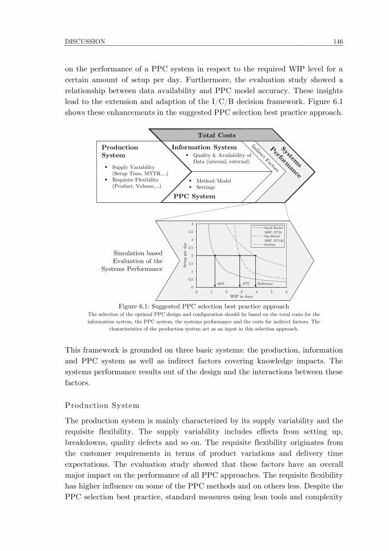
DISCUSSION 146
on the performance of a PPC system in respect to the required WIP level for a
certain amount of setup per day. Furthermore, the evaluation study showed a
relationship between data availability and PPC model accuracy. These insights
lead to the extension and adaption of the I/C/B decision framework. Figure 6.1
shows these enhancements in the suggested PPC selection best practice approach.
Figure 6.1: Suggested PPC selection best practice approach
The selection of the optimal PPC design and configuration should be based on the total costs for the
information system, the PPC system, the systems performance and the costs for indirect factors. The
characteristics of the production system act as an input in this selection approach.
This framework is grounded on three basic systems: the production, information
and PPC system as well as indirect factors covering knowledge impacts. The
systems performance results out of the design and the interactions between these
factors.
Production System
The production system is mainly characterized by its supply variability and the
requisite flexibility. The supply variability includes effects from setting up,
breakdowns, quality defects and so on. The requisite flexibility originates from
the customer requirements in terms of product variations and delivery time
expectations. The evaluation study showed that these factors have an overall
major impact on the performance of all PPC approaches. The requisite flexibility
has higher influence on some of the PPC methods and on others less. Despite the
PPC selection best practice, standard measures using lean tools and complexity
Information System
PPC System
Quality & Availability of Data (internal, external)
Method/Model Settings
Production System
Supply Variability (Setup Time, MTTR,…)
Requisite Flexibility (Product, Volume,…)
Simulation based Evaluation of the
Systems Performance
Total Costs
0
0,5
1
1,5
2
2,5
3
3,5
4
0 1 2 3 4 5 6
Set
up p
er d
ay
WIP in days
Small Bucket
MRP, PC24Big Bucket
MRP, PC120Kanban
-27%-68% Reference
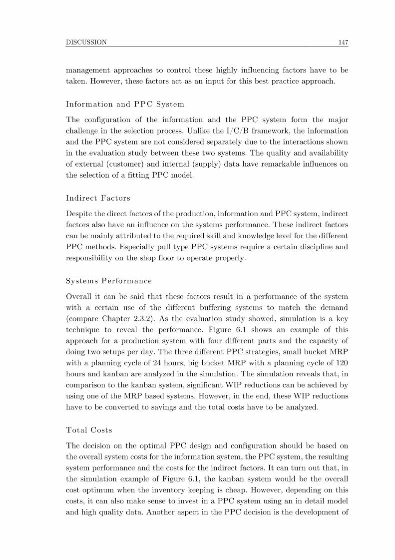
DISCUSSION 147
management approaches to control these highly influencing factors have to be
taken. However, these factors act as an input for this best practice approach.
Information and PPC System
The configuration of the information and the PPC system form the major
challenge in the selection process. Unlike the I/C/B framework, the information
and the PPC system are not considered separately due to the interactions shown
in the evaluation study between these two systems. The quality and availability
of external (customer) and internal (supply) data have remarkable influences on
the selection of a fitting PPC model.
Indirect Factors
Despite the direct factors of the production, information and PPC system, indirect
factors also have an influence on the systems performance. These indirect factors
can be mainly attributed to the required skill and knowledge level for the different
PPC methods. Especially pull type PPC systems require a certain discipline and
responsibility on the shop floor to operate properly.
Systems Performance
Overall it can be said that these factors result in a performance of the system
with a certain use of the different buffering systems to match the demand
(compare Chapter 2.3.2). As the evaluation study showed, simulation is a key
technique to reveal the performance. Figure 6.1 shows an example of this
approach for a production system with four different parts and the capacity of
doing two setups per day. The three different PPC strategies, small bucket MRP
with a planning cycle of 24 hours, big bucket MRP with a planning cycle of 120
hours and kanban are analyzed in the simulation. The simulation reveals that, in
comparison to the kanban system, significant WIP reductions can be achieved by
using one of the MRP based systems. However, in the end, these WIP reductions
have to be converted to savings and the total costs have to be analyzed.
Total Costs
The decision on the optimal PPC design and configuration should be based on
the overall system costs for the information system, the PPC system, the resulting
system performance and the costs for the indirect factors. It can turn out that, in
the simulation example of Figure 6.1, the kanban system would be the overall
cost optimum when the inventory keeping is cheap. However, depending on this
costs, it can also make sense to invest in a PPC system using an in detail model
and high quality data. Another aspect in the PPC decision is the development of
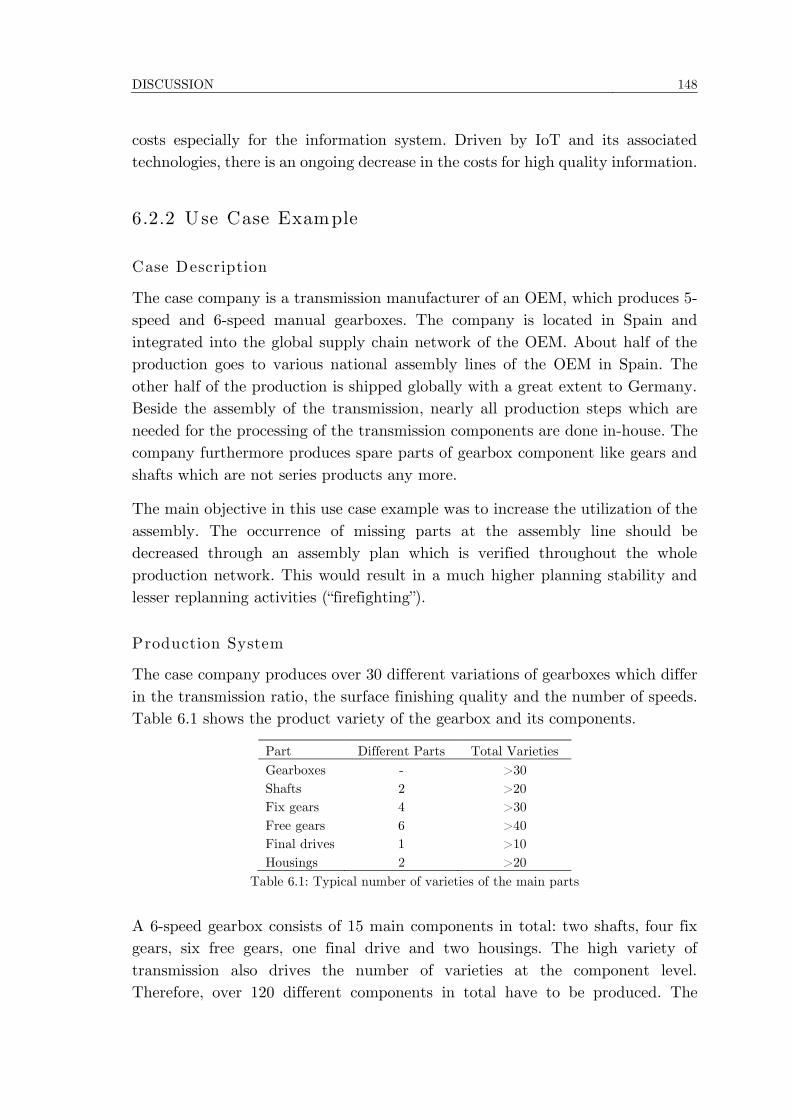
DISCUSSION 148
costs especially for the information system. Driven by IoT and its associated
technologies, there is an ongoing decrease in the costs for high quality information.
6.2.2 Use Case Example
Case Description
The case company is a transmission manufacturer of an OEM, which produces 5-
speed and 6-speed manual gearboxes. The company is located in Spain and
integrated into the global supply chain network of the OEM. About half of the
production goes to various national assembly lines of the OEM in Spain. The
other half of the production is shipped globally with a great extent to Germany.
Beside the assembly of the transmission, nearly all production steps which are
needed for the processing of the transmission components are done in-house. The
company furthermore produces spare parts of gearbox component like gears and
shafts which are not series products any more.
The main objective in this use case example was to increase the utilization of the
assembly. The occurrence of missing parts at the assembly line should be
decreased through an assembly plan which is verified throughout the whole
production network. This would result in a much higher planning stability and
lesser replanning activities (“firefighting”).
Production System
The case company produces over 30 different variations of gearboxes which differ
in the transmission ratio, the surface finishing quality and the number of speeds.
Table 6.1 shows the product variety of the gearbox and its components.
Part Different Parts Total Varieties
Gearboxes - >30
Shafts 2 >20
Fix gears 4 >30
Free gears 6 >40
Final drives 1 >10
Housings 2 >20
Table 6.1: Typical number of varieties of the main parts
A 6-speed gearbox consists of 15 main components in total: two shafts, four fix
gears, six free gears, one final drive and two housings. The high variety of
transmission also drives the number of varieties at the component level.
Therefore, over 120 different components in total have to be produced. The
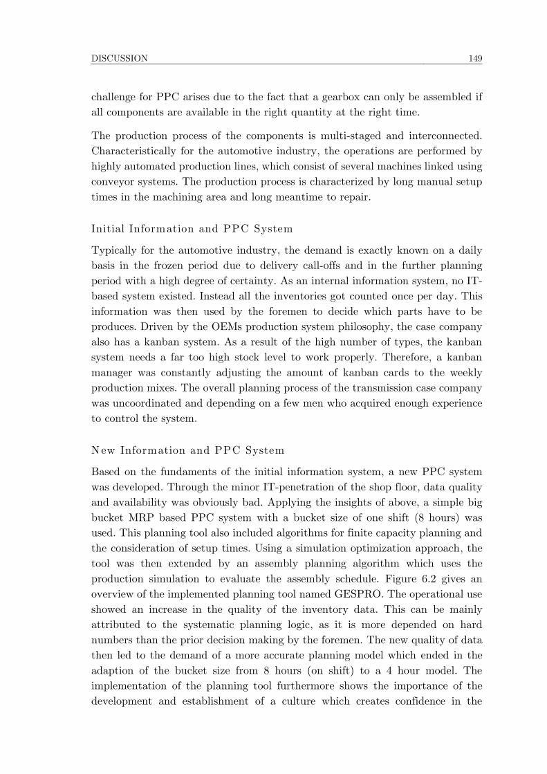
DISCUSSION 149
challenge for PPC arises due to the fact that a gearbox can only be assembled if
all components are available in the right quantity at the right time.
The production process of the components is multi-staged and interconnected.
Characteristically for the automotive industry, the operations are performed by
highly automated production lines, which consist of several machines linked using
conveyor systems. The production process is characterized by long manual setup
times in the machining area and long meantime to repair.
Initial Information and PPC System
Typically for the automotive industry, the demand is exactly known on a daily
basis in the frozen period due to delivery call-offs and in the further planning
period with a high degree of certainty. As an internal information system, no IT-
based system existed. Instead all the inventories got counted once per day. This
information was then used by the foremen to decide which parts have to be
produces. Driven by the OEMs production system philosophy, the case company
also has a kanban system. As a result of the high number of types, the kanban
system needs a far too high stock level to work properly. Therefore, a kanban
manager was constantly adjusting the amount of kanban cards to the weekly
production mixes. The overall planning process of the transmission case company
was uncoordinated and depending on a few men who acquired enough experience
to control the system.
New Information and PPC System
Based on the fundaments of the initial information system, a new PPC system
was developed. Through the minor IT-penetration of the shop floor, data quality
and availability was obviously bad. Applying the insights of above, a simple big
bucket MRP based PPC system with a bucket size of one shift (8 hours) was
used. This planning tool also included algorithms for finite capacity planning and
the consideration of setup times. Using a simulation optimization approach, the
tool was then extended by an assembly planning algorithm which uses the
production simulation to evaluate the assembly schedule. Figure 6.2 gives an
overview of the implemented planning tool named GESPRO. The operational use
showed an increase in the quality of the inventory data. This can be mainly
attributed to the systematic planning logic, as it is more depended on hard
numbers than the prior decision making by the foremen. The new quality of data
then led to the demand of a more accurate planning model which ended in the
adaption of the bucket size from 8 hours (on shift) to a 4 hour model. The
implementation of the planning tool furthermore shows the importance of the
development and establishment of a culture which creates confidence in the
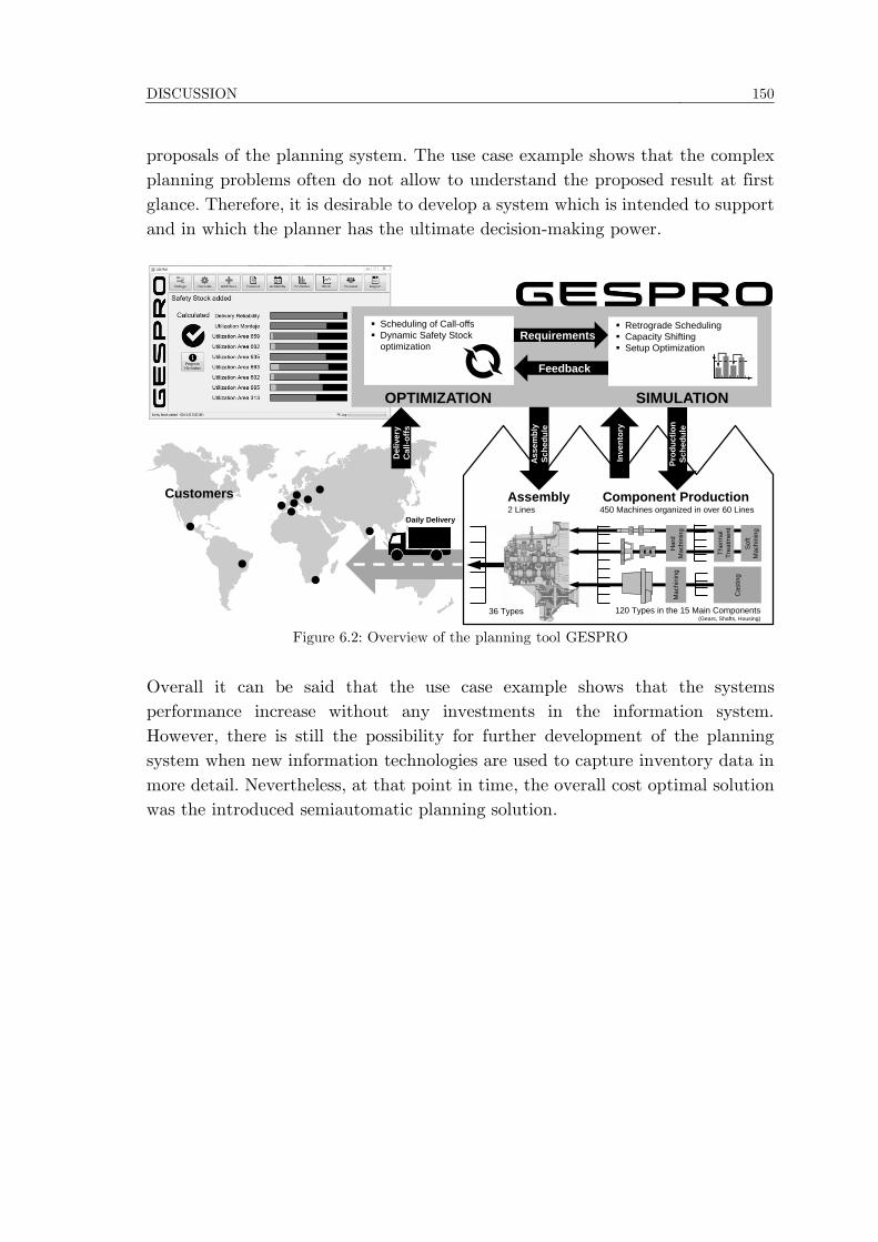
DISCUSSION 150
proposals of the planning system. The use case example shows that the complex
planning problems often do not allow to understand the proposed result at first
glance. Therefore, it is desirable to develop a system which is intended to support
and in which the planner has the ultimate decision-making power.
Figure 6.2: Overview of the planning tool GESPRO
Overall it can be said that the use case example shows that the systems
performance increase without any investments in the information system.
However, there is still the possibility for further development of the planning
system when new information technologies are used to capture inventory data in
more detail. Nevertheless, at that point in time, the overall cost optimal solution
was the introduced semiautomatic planning solution.
Hard
Machin
ing
Machin
ing
Therm
al
Tre
atm
ent
Soft
Machin
ing
Casting
Assembly Component Production
36 Types 120 Types in the 15 Main Components(Gears, Shafts, Housing)
2 Lines 450 Machines organized in over 60 Lines
Customers
Daily Delivery
OPTIMIZATION SIMULATION
Scheduling of Call-offs
Dynamic Safety Stock
optimization
Retrograde Scheduling
Capacity Shifting
Setup Optimization
Requirements
Feedback
Inve
nto
ry
As
se
mb
ly
Sch
ed
ule
Pro
du
cti
on
Sch
ed
ule
Deli
ve
ry
Call
-off
s
DISCUSSION 151
6.3 Lessons Learned
The field of PPC is strongly coined by thoughts of a close to religious level of on
the one hand the lean and on the other hand the IT believers. These two faith
groups are highly convinced of their worldview with only little scope of dialogue.
However, science and also practice shows us that IT is no muda92 and we need
collaboration between these two movements. Both the information and the
planning system must be selected wisely to ensure a cost optimal overall
performance. Another often claimed requirement for a PPC system is the
traceability of the planning decisions. Therefore, visual representations of the
planning results can be especially useful. Another aspect is the possibility and the
incentives for continuous improvements of the PPS system. Furthermore, the
human integration in the decision making is an important issue. The trend to
autonomous decision making might have negative aspects on the cognitive skills
of a production planner. Nowadays, the production planner has results of
predictions and decisions of the past in his head, which will be useful for his future
actions. These mental response relationships might get lost in fully autonomous
operated systems and in case of extracurricular events, a human might not be
able to take over the decision making task any more.
92 Muda (無駄) is a Japanese word meaning futility; uselessness; idleness; superfluity; waste; wastage.
Conclusion
Thinking is the hardest work there is, which is
probably the reason why so few engage in it. Henry Ford (1863 – 1947)
After years of lean production, a new hype is flooding the manufacturing industry.
Informatization of the shop floor and the supply chains using IoT and several
associated enabling technologies is now the rage. Several initiatives such as the
Physical Internet, the Industrial Internet or also Industry 4.0 were started and
have the attention of the top management. Consultants and white papers promise
significant efficiency increases93 through the new possibilities of informatization
in manufacturing. Several companies expect a better production planning and
control and a higher flexibility through the increasing availability of high quality
data. It is expected that powerful, autonomous algorithms will control the
production based on the available real time information and will directly interact
with the machines as CPS in the future.
Nevertheless, the production planning and control real life, especially in the
automotive supply industry, is nowadays a totally different one. I experienced
that after years of consulting, many production planners acquired a strong believe
in one of the two big production paradigms push and pull, without an in-detail
93 according to a Strategy& and PricewaterhouseCoopers (2014) study the annual increase in the resource
efficiency will be 3.3% on average across all industries.
C H A P T E R
CONCLUSION 153
understanding of the underlying methods and the influencing factors.
Furthermore, information quality is still far away from high quality and real time.
As a result of the often poor data quality, PPC decisions are based on averages
or estimates and simple planning models which then results in inaccurate planning
results. This discrepancy of the inventory and demand data between information
systems and the real physical flow of goods is a well-known phenomenon.
7.1 Research Question
This thesis presents a simulation based evaluation study which analyzed the
impacts of informatization on PPC. This evaluation shows that real time
information is not absolutely necessary. A relation between modelling accuracy
and data quality can be seen. Without the right planning model, real time data
can be worthless. The simulation based analysis of the PPC systems behavior
proofed to be a valuable approach in the selection of the right PPC setting for a
given production system. In the evaluation, it turned out that especially the
product flexibility plays a major role in the selection of an appropriate PPC
strategy. The evaluation results also show that significant improvements can be
achieved by using the right planning model and the right settings. I think that a
shift away from the stereotypical thinking of push or pull type PPC systems
towards an understanding of the underlying algorithms and the influencing
parameters is necessary. The insights and the presented best practice for the
selection of the right PPC strategy of Chapter 6 are a valued step on the road to
this understanding.
7.2 Further Research
Nevertheless, further research in this area is necessary. One potential topic is the
hierarchy of the PPC decision making. The analyzed methods in this thesis are
focusing only on one specific line. Due to the limitations of the used simulation
model, it was not possible to evaluate the network behavior of these different
methods. Thereby, the trend to more decentralized decision making instead of the
classical centralized top down approach is of special interest. I assume that there
is the demand of both elements, centralized and decentralized, in PPC. The right
amount of these elements and the overall design must be investigated in further
research activities.
List of Figures
Figure 1.1: Brand concentration in the European automotive industry .............. 2
Figure 1.2: Development of the model range of Audi .......................................... 3
Figure 1.3: Process focus area of the thesis ......................................................... 8
Figure 1.4: Overview of the approach of this thesis........................................... 10
Figure 2.1: Classical logistics classification along the supply chain ................... 15
Figure 2.2: Development of production management ........................................ 22
Figure 2.3: Links between fundamental and operational objectives ................... 25
Figure 2.4: Influence of variability and the OM-triangle ................................... 29
Figure 2.5: Linkages between the various flexibilities ........................................ 36
Figure 2.6: Hierarchy of flexibility dimensions .................................................. 36
Figure 2.7: Distinction between flexibility and adaptability .............................. 37
Figure 2.8: Relationships between agility, adaptability and flexibility .............. 38
Figure 3.1: Relationships between data, information, knowledge and wisdom .. 41
Figure 3.2: Computer integrated manufacturing wheel ..................................... 45
Figure 3.3: Computer integrated manufacturing Y-model ................................. 46
Figure 3.4: Digital factory processes .................................................................. 47
Figure 3.5: Conventional and cooperative approach to decision-making ........... 54
Figure 4.1: Total planning approach ................................................................. 66
Figure 4.2: Connecting planning approach ........................................................ 66
Figure 4.3: Rolling horizon planning ................................................................. 66
Figure 4.4: Generic hierarchical PPC process .................................................... 67
Figure 4.5: Material and information flow in a MRP production system .......... 71
LIST OF FIGURES 155
Figure 4.6: Material and information flow in a JIT production system ............. 71
Figure 4.7: Evolution of PPC Systems .............................................................. 72
Figure 4.8: Costs in the EOQ model ................................................................. 74
Figure 4.9: Big and small bucket models ........................................................... 75
Figure 4.10: Typical modules of an APS software ............................................. 82
Figure 4.11: Toyota’s view of inventory ............................................................ 85
Figure 4.12: Single card kanban system ............................................................ 86
Figure 5.1: Modeling Process ............................................................................. 98
Figure 5.2: Application fields of modeling and simulation techniques in PPC .. 98
Figure 5.3: Concept of simulation optimization ............................................... 101
Figure 5.4: Motivations for the evaluation ...................................................... 101
Figure 5.5: Different types of routing in manufacturing systems ..................... 102
Figure 5.6: Scope of the evaluation study ........................................................ 104
Figure 5.7: Two examples of applications of the evaluation model in a multistage
and multicomponent production network ........................................................ 105
Figure 5.8: General structure of the evaluation model .................................... 106
Figure 5.9: Different demand mixes ................................................................. 107
Figure 5.10: Example of a sampled demand (4P, SM) .................................... 107
Figure 5.11: Demand changes in the forecast .................................................. 108
Figure 5.12: Conveyor model ........................................................................... 109
Figure 5.13: Variability of the manufacturing line .......................................... 109
Figure 5.14: Repair time histogram of the low/high variability scenarios ....... 110
Figure 5.15: Example of the influence of the lead time ................................... 111
Figure 5.16: Length of the warm-up period using a kanban system ................ 112
Figure 5.17: Exchanged data between the DES and the MRP-based Algorithm
........................................................................................................................ 113
Figure 5.18: Example of the small bucket MRP algorithm.............................. 114
Figure 5.19: Flowchart of the small bucket MRP core algorithm .................... 115
Figure 5.20: Relationship of maximum inventory range and setup counter ..... 116
Figure 5.21: Flowchart of the maximum range optimization of the small bucket
MRP algorithm ............................................................................................... 116
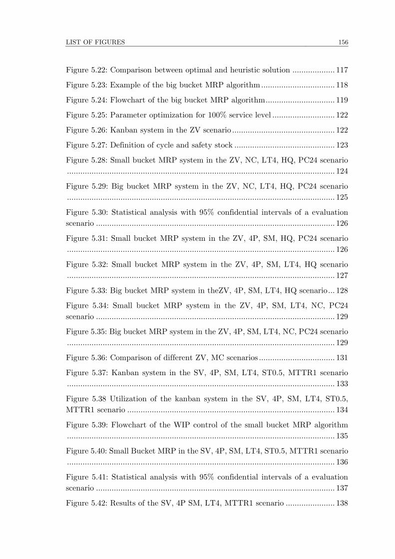
LIST OF FIGURES 156
Figure 5.22: Comparison between optimal and heuristic solution ................... 117
Figure 5.23: Example of the big bucket MRP algorithm ................................. 118
Figure 5.24: Flowchart of the big bucket MRP algorithm ............................... 119
Figure 5.25: Parameter optimization for 100% service level ............................ 122
Figure 5.26: Kanban system in the ZV scenario .............................................. 122
Figure 5.27: Definition of cycle and safety stock ............................................. 123
Figure 5.28: Small bucket MRP system in the ZV, NC, LT4, HQ, PC24 scenario
........................................................................................................................ 124
Figure 5.29: Big bucket MRP system in the ZV, NC, LT4, HQ, PC24 scenario
........................................................................................................................ 125
Figure 5.30: Statistical analysis with 95% confidential intervals of a evaluation
scenario ........................................................................................................... 126
Figure 5.31: Small bucket MRP system in the ZV, 4P, SM, HQ, PC24 scenario
........................................................................................................................ 126
Figure 5.32: Small bucket MRP system in the ZV, 4P, SM, LT4, HQ scenario
........................................................................................................................ 127
Figure 5.33: Big bucket MRP system in theZV, 4P, SM, LT4, HQ scenario ... 128
Figure 5.34: Small bucket MRP system in the ZV, 4P, SM, LT4, NC, PC24
scenario ........................................................................................................... 129
Figure 5.35: Big bucket MRP system in the ZV, 4P, SM, LT4, NC, PC24 scenario
........................................................................................................................ 129
Figure 5.36: Comparison of different ZV, MC scenarios .................................. 131
Figure 5.37: Kanban system in the SV, 4P, SM, LT4, ST0.5, MTTR1 scenario
........................................................................................................................ 133
Figure 5.38 Utilization of the kanban system in the SV, 4P, SM, LT4, ST0.5,
MTTR1 scenario ............................................................................................. 134
Figure 5.39: Flowchart of the WIP control of the small bucket MRP algorithm
........................................................................................................................ 135
Figure 5.40: Small Bucket MRP in the SV, 4P, SM, LT4, ST0.5, MTTR1 scenario
........................................................................................................................ 136
Figure 5.41: Statistical analysis with 95% confidential intervals of a evaluation
scenario ........................................................................................................... 137
Figure 5.42: Results of the SV, 4P SM, LT4, MTTR1 scenario ...................... 138

LIST OF FIGURES 157
Figure 5.43: Results of the SV, 4P SM, LT4, MTTR4 scenario ...................... 139
Figure 5.44: Comparison of different SV, MC, MTTR1 scenarios ................... 140
Figure 6.1: Suggested PPC selection best practice approach ........................... 146
Figure 6.2: Overview of the planning tool GESPRO ....................................... 150
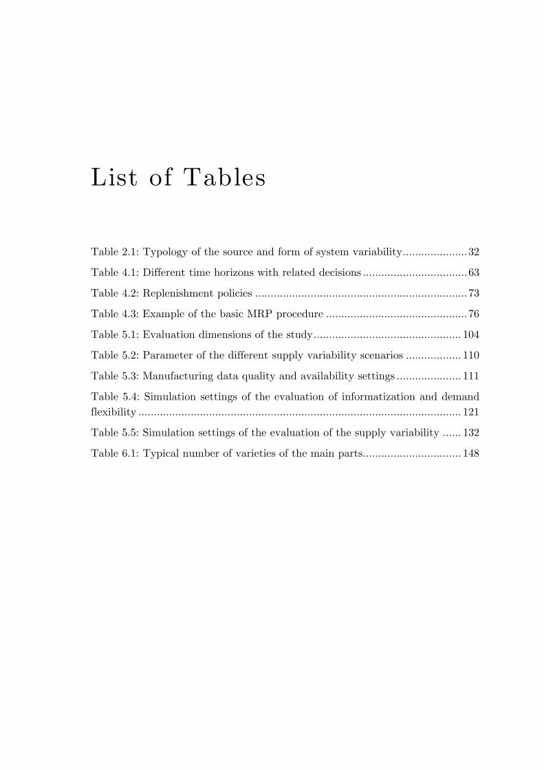
List of Tables
Table 2.1: Typology of the source and form of system variability ..................... 32
Table 4.1: Different time horizons with related decisions .................................. 63
Table 4.2: Replenishment policies ..................................................................... 73
Table 4.3: Example of the basic MRP procedure .............................................. 76
Table 5.1: Evaluation dimensions of the study ................................................ 104
Table 5.2: Parameter of the different supply variability scenarios .................. 110
Table 5.3: Manufacturing data quality and availability settings ..................... 111
Table 5.4: Simulation settings of the evaluation of informatization and demand
flexibility ......................................................................................................... 121
Table 5.5: Simulation settings of the evaluation of the supply variability ...... 132
Table 6.1: Typical number of varieties of the main parts................................ 148
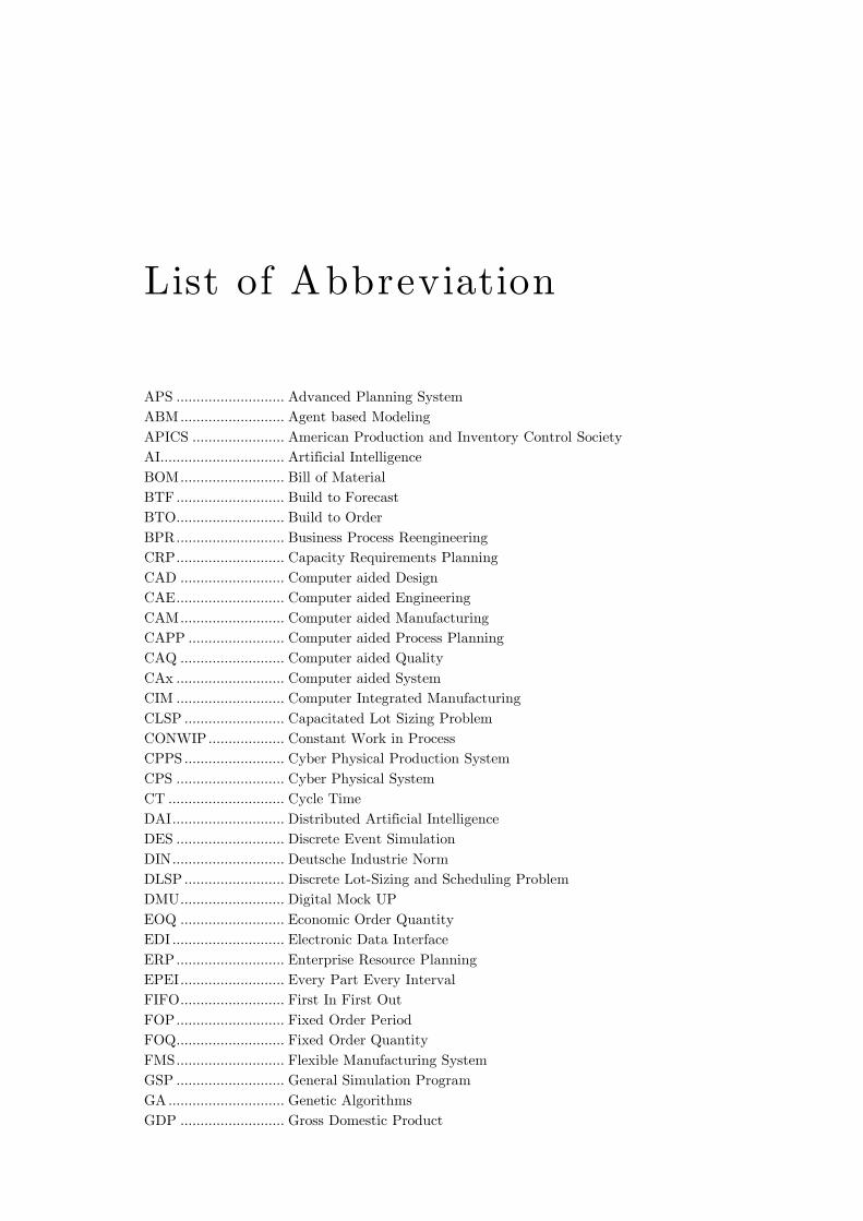
List of Abbreviation
APS ........................... Advanced Planning System
ABM .......................... Agent based Modeling
APICS ....................... American Production and Inventory Control Society
AI............................... Artificial Intelligence
BOM .......................... Bill of Material
BTF ........................... Build to Forecast
BTO ........................... Build to Order
BPR ........................... Business Process Reengineering
CRP ........................... Capacity Requirements Planning
CAD .......................... Computer aided Design
CAE ........................... Computer aided Engineering
CAM .......................... Computer aided Manufacturing
CAPP ........................ Computer aided Process Planning
CAQ .......................... Computer aided Quality
CAx ........................... Computer aided System
CIM ........................... Computer Integrated Manufacturing
CLSP ......................... Capacitated Lot Sizing Problem
CONWIP ................... Constant Work in Process
CPPS ......................... Cyber Physical Production System
CPS ........................... Cyber Physical System
CT ............................. Cycle Time
DAI ............................ Distributed Artificial Intelligence
DES ........................... Discrete Event Simulation
DIN ............................ Deutsche Industrie Norm
DLSP ......................... Discrete Lot-Sizing and Scheduling Problem
DMU .......................... Digital Mock UP
EOQ .......................... Economic Order Quantity
EDI ............................ Electronic Data Interface
ERP ........................... Enterprise Resource Planning
EPEI .......................... Every Part Every Interval
FIFO .......................... First In First Out
FOP ........................... Fixed Order Period
FOQ ........................... Fixed Order Quantity
FMS ........................... Flexible Manufacturing System
GSP ........................... General Simulation Program
GA ............................. Genetic Algorithms
GDP .......................... Gross Domestic Product
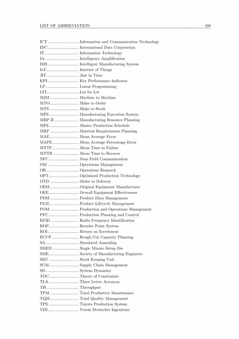
LIST OF ABBREVIATION 160
ICT ............................ Information and Communication Technology
IDC ............................ International Data Corporation
IT ............................... Information Technology
IA............................... Intelligence Amplification
IMS ............................ Intelligent Manufacturing System
IoT ............................. Internet of Things
JIT ............................. Just in Time
KPI ............................ Key Performance Indicator
LP .............................. Linear Programming
LFL ............................ Lot for Lot
M2M .......................... Machine to Machine
MTO .......................... Make to Order
MTS ........................... Make to Stock
MES ........................... Manufacturing Execution System
MRP II ...................... Manufacturing Resource Planning
MPS ........................... Master Production Schedule
MRP .......................... Material Requirements Planning
MAE .......................... Mean Average Error
MAPE ........................ Mean Average Percentage Error
MTTF ........................ Mean Time to Failure
MTTR ....................... Mean Time to Recover
NFC ........................... Near Field Communication
OM ............................ Operations Management
OR ............................. Operations Research
OPT ........................... Optimized Production Technology
OTD .......................... Order to Delivery
OEM .......................... Original Equipment Manufacturer
OEE ........................... Overall Equipment Effectiveness
PDM .......................... Product Data Management
PLM........................... Product Lifecycle Management
POM .......................... Production and Operations Management
PPC ........................... Production Planning and Control
RFID ......................... Radio Frequency Identification
ROP ........................... Reorder Point System
ROI ............................ Return on Investment
RCCP ........................ Rough Cut Capacity Planning
SA .............................. Simulated Annealing
SMED ........................ Single Minute Setup Die
SME ........................... Society of Manufacturing Engineers
SKU ........................... Stock Keeping Unit
SCM ........................... Supply Chain Management
SD .............................. System Dynamics
TOC........................... Theory of Constraints
TLA ........................... Three Letter Acronym
TH ............................. Throughput
TPM .......................... Total Productive Maintenance
TQM .......................... Total Quality Management
TPS ........................... Toyota Production System
VDI ............................ Verein Deutscher Ingenieure

LIST OF ABBREVIATION 161
WSAN ....................... Wireless Sensor and Actuator Network
WIP ........................... Work in Process
Evaluation M odel 2P, 4P, 8P ................. Part Range (2, 4, 8 different parts)
SM, DM ..................... Demand Mix (static, dynamic mix)
NC, FC, MC .............. possible Changes in Forecast (no, few, many changes)
ZV, SV ....................... Supply Variability (zero, supply variability with ST and MTTR)
ST0.5, ST1, ST2 ........ Setup Time (0.5, 1, 2 hours)
MTTR1, MTTR4 ...... Mean Time to Repair (1, 4 hours)
LT4, LT12 ................. Lead Time (4, 12 hours)
HQ, MQ, PQ ............. Internal Information Quality (high, medium, poor information quality)
PC1, PC24, PC120 .... Internal Information Availability (1, 24, 120 hours planning cycle)
Bibliography
Ackoff, R. L., 1989. From Data to Wisdom. Journal of Applies Systems Analysis,
Volume 16, pp. 3-9.
Anthony, R. N., 1965. Planning and Control Systems. A Framework for Analysis.
Boston: Division of Research Graduate School of Business Administration
Harvard University.
Apel, D., Behme, W., Eberlein, R. & Merighi, C., 2010. Datenqualität erfolgreich
steuern: Praxislösungen für Business-Intelligence-Projekte. 2nd ed. München,
Wien: Hanser.
APICS, 2013. APICS Dictionary. 14 ed. Chicago: APICS.
Arnold, D., Isermann, H., Kuhn, A. & Tempelmeier, H., 2003. Handbuch Logistik.
Berlin/Heidelberg: Springer.
Ashby, R. W., 1956. An Introduction to Cybernetics. London: Methuen.
Atzori, L., Iera, A. & Morabito, G., 2010. The Internet of Things: A Survey.
Computer Networks, Volume 54, pp. 2787-2805.
Audi, 2012. Audi Deutschland. [Online]
Available at: www.audi.de
[Accessed 12 10 2012].
Axsäter, S. & Rosling, K., 1994. Multi-Level Production-Inventory Control:
Material Requirements Planning or Reorder Policies?. European Journal of
Operational Research, 75(2), pp. 405-412.
Bainbridge, L., 1983. Ironies of Automation. Automatica, 19(6), pp. 775-779.
Barbey, H. P., 2010. Auslegung von Kanbansteuerungen bei starken
Produktionsschwankungen mit Hilfe von disketer Simulation. Karlsruhe, ASIM
Simulation in Production and Logistics.
BIBLIOGRAPHY 163
Batini, C. & Scannapieca, M., 2006. Data Quality. Concepts, Methodologies and
Techniques. Berlin, Heidelberg: Springer.
Bauernhansl, T., 2014. Die Vierte Industrielle Revolution: Der Weg in ein
wertschaffendes Produktionsparadigma. In: T. Bauernhansl, M. Hompel & B.
Vogel-Heuser, eds. Industrie 4.0 in Produktion, Automatisierung und Logistik.
Wiesbaden: Springer, pp. 5-35.
Bellinger, G., Castro, D. & Mills, A., 2004. Data, Information, Knowledge, and
Wisdom. s.l.:s.n.
Benton, W. C. & Shin, H., 1998. Manufacturing Planning and Control: The
Evolution of MRP and JIT Integration. European Journal of Operational
Research, Volume 110, pp. 411-440.
Bernardes, E. S. & Hanna, M. D., 2009. A Theoretical Review on Flexibility,
Agility and Responsiveness in the Operations Management Literature.
International Journal of Operations & Production Management, 29(1), pp. 30-53.
Bildstein, A. & Seidelmann, J., 2014. Industrie 4.0-Readiness: Migration zur
Industrie 4.0-Fertigung. In: T. Bauernhansl, M. Hompel & B. Vogel-Heuser, eds.
Industrie 4.0 in Produktion, Automatisierung und Logistik. Wiesbaden: Spinger,
pp. 581-591.
Boston Consulting Group, 2015. Industry 4.0: The Future of Productivity and
Growth in Manufacturing Industries, s.l.: Boston Consulting Group.
Box, G. E. & Draper, N. R., 1987. Empirical Model-Building and Response
Surfaces. Hoboken, New Jersey: John Wiley & Sons.
Bröder, P., 2014. Industrie 4.0 and Big Data: Kritische Reflexion
Forschungspolitischer Visionen, Siegen: Universität Siegen.
Buffon, G., 1777. Essais d’Arithmétique morale. Histoire Naturelle, Volume 4,
pp. 46-123.
Buzacott, J. A. & Shanthikumar, J. G., 1994. Safety Stock versus Safety Time in
MRP Controlled Production Systems. Management Science, 40(12), pp. 1678-
1689.
Carson, Y. & Maria, A., 1997. Simulation Optimization: Methods and
Applications. Atlanta, Proceedings of the 1997 Winter Simulation Conference.
Castells, M., 1996. The Rise of the Network Society: The Information Age:
Economy, Society, and Culture. Oxford: Blackwell.
BIBLIOGRAPHY 164
Chan, F. T. & Wang, Z., 2014. Robust Production Control Policy for a Multiple
Machine and Multiple Product-types Manufacturing System with Inventory
Inaccuracy. International Journal of Production Research, 52(16), pp. 4803-4819.
Christo, C. & Cardeira, C., 2007. Trends in Intelligent Manufacturing Systems.
Vigo, Spain, IEEE International Symposium on Industrial Electronics.
Chryssolouris, G. et al., 2009. Digital Manufacturing: History, Perspectives, and
Outlook. Journal of Engineering Manufacture, Volume 223, pp. 451-462.
Clark, W., 1942. The Gantt Chart, a Working Tool of Management. 2 ed. London:
Sir Isaac Pitman & Sons.
Conway, R. W., Maxwell, W. L. & Miller, L. W., 1967. Theory of Scheduling.
Mineola: Dover Publications.
Dalkey, N. & Helmer, O., 1962. An Experimental Application of the Delphi
Method to the use of Experts. Santa Monica: RAND Corporation.
Dangelmaier, W., 2009. Theorie der Produktionsplanung und -steuerung. Berlin,
Heidelberg: Springer.
Davenport, T. H., 1997. Information Ecology: Mastering the Information and
Knowledge Environment. New York: Oxford University Press.
Davis, J. P., Eisenhardt, K. M. & Bingham, C. B., 2007. Development Theory
Through Simulation Methods. Academy of Management Review, 32(2), pp. 480-
499.
DeHoratius, N. & Raman, A., 2004. Inventory Record Inaccuracy: An Empirical
Analysis, Chicago: University of Chicago.
Deloitte, 2003. The Challenge of Complexity in Global Manufacturing, London:
Deloitte Touche Tohmatsu.
DeLone, W. H. & McLean, E. R., 1992. Information Systems Success: The Quest
for the Dependent Variable. Information Systems Research, 3(1), pp. 60-95.
Dickmann, P., 2009. Schlanker Materialfluss: mit Lean Production, Kanban und
Innovationen. 2nd ed. Berlin, Heidelberg: Springer.
DIN, 1968. Regelungstechnik und Steuerungstechnik. Begriffe und Benennungen.
Berlin: Beuth.
Drucker, P. F., 1954. The Practice of Management. New York: Harper & Row.
Edelkamp, S. & Schrödl, S., 2012. Heuristic Search: Theory and Application.
Waltham: Morgan Kaufmann.
BIBLIOGRAPHY 165
Edwards, J. N., 1983. MRP and Kanban – American Style. APICS 26th
Conference Proceedings, pp. 586-603.
Encyclopedia Britannica, 2014. [Online]
Available at: http://www.britannica.com/EBchecked/topic/346422/logistics
[Accessed 6 May 2014].
Eppler, M. J., 2006. Managing Information Quality. Increasing the Value of
Information in Knowledge-intensive Products and Processes. Heidelberg:
Springer.
Erlach, K., 2010. Wertstromdesign. 2nd ed. Berlin Heidelberg: Springer.
Evans, P. C. & Annunziata, M., 2012. Industrial Internet: Pushing the Boundaries
of Minds and Machines, s.l.: s.n.
Fleisch, E. & Tellkamp, C., 2005. Inventory Inaccuracy and Supply Chain
Performance a Simulation Study of a Retail Supply Chain. Journal of Production
Economics, 95(3), pp. 373-385.
Ford, H., 1926. Today and Tomorrow. s.l.:s.n.
Forrester, J. W., 1961. Industrial Dynamics. Cambridge: MIT Press.
Frantz, F. K., 1995. A Taxonomy of Model Abstraction Techniques. New York,
Proceedings of the 1995 Winter Simulation Conference.
Gantt, H. L., 1919. Organizing for Work. New York: Harcourt, Brace, and Howe.
Gaury, E., Pierreval, H. & Kleijnen, J., 2000. An Evolutionary Approach to Select
a Pull System among Kanban, Conwip and Hybrid. Journal of Intelligent
Manufacturing, Volume 11, pp. 157-167.
Goldmann, S. L., Nagel, R. N. & Preiss, K., 1995. Agile Competitors and Virtual
Organizations: Strategies for Enriching Customers. New York: Van Nostrand
Reinhold.
Goldratt, E. M. & Cox, J., 1984. The Goal: A Process of Ongoing Improvement.
Croton-on-Hudson: North River Press.
Goldsman, D., Nance, R. E. & Wilson, J. R., 2010. A Brief History of Simulation
Revisited, Raleigh: North Carolina State University.
Graves, S. C., Rinnooy Kan, A. H. G. & Zipkin, P. H., 2002. Logistics of
Production and Inventory. 4th ed. Amsterdam: Elsevier.
Greeno, J., 1978. Natures of Problem-Solving Ability. Handbook of learning and
Cognitive Processes. Hillsdale: Lawrence Erlbaum.
BIBLIOGRAPHY 166
Groover, M. P., 2007. Automation, Production Systems, and Computer-Integrated
Manufacturing. 3rd ed. Upper Saddle River: Prentice Hall Press.
Gutenberg, E., 1951. Grundlagen der Betriebswirtschaftslehre. Band 1: Die
Produktion. Berlin: Springer.
Hall, R. W., 1981. Driving the Productivity Machine: Production and Control in
Japan. s.l.:APICS.
Harrington, J., 1973. Computer Integrated Manufacturing. Malabar, Florida:
Krieger Publishing.
Harris, F. W., 1913. How Many Parts to Make at Once. Factory, The Magazine
of Management, 10(2), pp. 135-136.
Hax, A. C. & Meal, H. C., 1973. Hierarchical integration of production planning
and scheduling. Cambridge: Massachusetts Institute of Technology.
Hayes, R. H. & Wheelwright, S. C., 1979. Link Manufacturing Process and
Product Life Cycles. Harvard Business Review, pp. 133-140.
Hering, N., Meißner, J. & Reschke, J., 2013. ProSense - Untersuchung
"Produktion am Standort Deutschland 2013". Zeitschrift für wirtschaftlichen
Fabrikbetrieb, 108(12), pp. 995-998.
Herrmann, J. W., 2006. A History of Production Scheduling. In: Handbook of
Production Scheduling. s.l.:Springer, pp. 1-22.
Holweg, M. & Pil, F. K., 2004. The Second Century: Reconnecting Customer and
Value Chain Through Build-To-Order; Moving Beyond Mass and Lean
Production in the Auto Industry. Cambridge: MIT Press.
Hompel, M. & Henke, M., 2014. Logistik 4.0. In: T. Bauernhansl, M. Hompel &
B. Vogel-Heuser, eds. Industrie 4.0 in Produktion, Automatisierung und Logistik.
Wiebaden: Springer, pp. 615-625.
Hopp, W. J. & Spearman, M. L., 2004. To Pull or not to Pull: What is the
Question?. Manufacturing & Service Operations Management, 6(2), pp. 133-148.
Hopp, W. & Spearman, M., 2008. Factory Physics: Foundations of Manufacturing
Management. New York: McGraw-Hill.
International Data Corporation, 2014. The Digital Universe of Opportunities, s.l.:
IDC.
Jelenik, M. & Goldhar, J., 1984. The Strategic Implications of the Factory of the
Future. Sloan Management Review, Volume 4, pp. 28-37.
BIBLIOGRAPHY 167
Jodlbauer, H. & Huber, A., 2008. Service-Level Performance of MRP, Kanban,
CONWIP and DBR due to Parameter Stability and Environmental Robustness.
International Journal of Production Research, 46(8), pp. 2179-2195.
Juran, J. M., 1989. Juran on Leadership in Quality: An Executive Handbook. New
York: The Free Press.
Juran, J. M., 1992. Juran on Quality by Design: The New Steps for Planning
Quality into Goods and Services: Planning, Setting and Reaching Quality Goals.
New York: The Free Press.
Kang, Y. & Gershwin, S. B., 2004. Information Inaccuracy in Inventory Systems
- Stock Loss and Stockout. IEE Transactions, Volume 37, pp. 843-859.
Karmarkar, U., 1988. Getting Control of Just in Time. Harvard Business Review,
67(5), pp. 122-131.
Kendall, D. G., 1953. Stochastic Processes Occurring in the Theory of Queues
and their Analysis by the Method of the Embedded Markov Chain. The Annals
of Mathematical Statistics, 24(3), pp. 338-354.
Kern, W., 1995. Handwörterbuch der Produktionswirtschaft. Stuttgart: Schäffer-
Poeschel.
Klassen, R. D. & Menor, L. J., 2007. The Process Management Triangle: An
Empirical Investigation of Process Trade-offs. Operations Management, Volume
25, pp. 1015-1034.
Klug, F., 2010. Logistikmanagement in der Automobilindustrie. Berlin Heidelberg:
Springer.
Koch, H., 1977. Aufgaben der Unternehmensplannung. Wiesbaden: Gabler.
Koren, Y., 2010. The Global Manufacturing Revolution. New Jersey: Wiley.
Koste, L. L. & Malhotra, M. K., 1999. A Theoretical Framework for Analyzing
the Dimensions of Manufacturing Flexibility. Journal of Operations Management,
18(1), pp. 75-93.
KPMG, 2010. Unternehmens- und Markenkonzentration in der europäischen
Automobilindustry, Stuttgart: KPMG.
Krajewski, L. J., King, B. E. & Ritzmann, L. P., 1987. Kanban, MRP and Shaping
the Manufacturing Environment. Management Science, 33(1), pp. 39-57.
BIBLIOGRAPHY 168
Krishnamurthy, A., Suri, R. & Vernon, M., 2000. Push Can Perform Better than
Pull for Flexible Manufacturing Systems with Multiple Products. s.l., Industrial
Engineering Research 2000 Conference Proceedings.
Krishnamurthy, A., Suri, R. & Vernon, M., 2004. Re-Examining the Performance
of MRP and Kanban Material Control Strategies for Multi-Product Flexible
Manufacturing Systems. International Journal of Flexible Manufacturing
Systems, Volume 16, pp. 123-150.
Krog, E. H. & Statkevich, K., 2008. Kundenorientierung und Integrationsfunction
der Logistk in der Supply Chain der Automobilindustrie. In: H. Baumgarten, ed.
Das Beste der Logistik. Berlin/Heidelberg: Springer.
Kühn, W., 2006. Digital Factory: Simulation Enhancing the Product and
Production Engineering Process. Monterey, Proceedings of the 2006 Winter
Simulation Conference.
Kumar, A. S. & Suresh, N., 2008. Production and Operations Management. 2 ed.
New Delhi: New Age International.
Law, A. M. & Kelton, D., 2000. Simulation Modeling and Analysis. 3rd ed. New
York: McGraw-Hill.
Lee, E. A., 2008. Cyber Physical Systems: Design Challenges. Orlando, 11th IEEE
International Symposium on Object Oriented Real-Time Distributed Computing.
Lee, H. L., 2002. Aligning Supply Chain Strategies with Product Uncertainties.
California Management Review, 44(3), pp. 105-119.
Lee, H. L., Padmanabhan, V. & Whang, S., 1997. Information Distortion in a
Supply Chain: The Bullwip Effect. Management Science, 43(4), pp. 546-558.
Lee, I., 2010. Cyber Physical Systems: The Next Computing Revolution,
Philadelphia: University of Pennsylvania.
Leitao, P., 2009. Agent-Based Distributed Manufacturing Control: A State-of-
the-Art Survey. Engineering Applications of Artificial Intelligence, Volume 22,
pp. 979-991.
Little, J. D., 1961. A Proof of the Queueing Formula L = λ W. Operations
Research, Volume 9, p. 383–387.
Little, J. D. & Graves, S. C., 2008. Little's Law. In: D. Chhajed & T. J. Lowe,
eds. Building Intuition: Insights from Basic Operations Management Models and
Principles. New York: Springer, p. 81 – 100.
BIBLIOGRAPHY 169
Lovejoy, W. S., 1998. Integrated Operations: A Proposal for Operations
Management Teaching and Research. Production and Operations Management,
7(2), pp. 106-123.
Luce, R. D. & Raiffa, H., 1957. Games and Decisions: Introduction and Critical
Survey. s.l.:Dover Publications.
Malik, F., 2002. Komplexität - was ist das?, s.l.: Cwarel Isaf Institute.
Marik, V. & McFarlane, D., 2005. Industrial Adoption of Agent-Based
Technologies. IEEE Intelligent Systems, 20(1), pp. 27-35.
Martin, J., 1965. Programming Real-Time Computer Systems. Englewood Cliffs:
Prentice-Hall.
März, L. & Krug, W., 2011. Simulation und Optimierung in Produktion und
Logistik. Berlin Heidelberg: Springer.
Matsuura, H., Kurosu, S. & Lehtimäki, A., 1995. Concepts, Practices and
Expectations of MRP, JIT and OPT in Finland and Japan. International Journal
of Production Economics, Volume 41, pp. 267-272.
McGilvray, D. & Thomas, G., 2008. Executing Data Quality Projects: Ten Steps
to Quality Data and Trusted Information. s.l.:Elsevier.
McKinsey & Company, 2013. The Road to 2020 and Beyond: What's Driving the
Global Automotive Industry?, Stuttgart: McKinsey & Company.
McKinsey & Company, 2014. Perspectives on Manufacturing, Disruptive
Technologies, and Industry 4.0, s.l.: McKinsey & Company.
Micklethwait, J. & Wooldridge, A., 1996. The Witch Doctors: Making Sense of
the Management Gurus. New York: Random House.
Minsky, M., 1988. Society of Mind. New York: Simon and Schuster.
Mönch, L., Fowler, J. W. & Mason, S. J., 2013. Production Planning and Control
for Semiconductor Wafer Fabrication Facilities. New York: Springer.
Monden, Y., 1984. A Simulation Analysis of the Japanese Just In Time Technique
(with Kanban) for a Multiline, Multistage Production System. Decision Science,
Volume 15, pp. 445-447.
Monostori, L., Vancza, J. & Kumara, S., 2006. Agent-Based Systems for
Manufacturing. Annals of the CIRP, 55(2), pp. 697-720.
BIBLIOGRAPHY 170
Montreuil, B., 2012. Physical Internet Manifesto: Transforming the way physical
objects are moved, stored, realized supplied and used, aiming towards greater
efficiency and sustainability, Quebec: Physical Internet Initiative.
Moore, G. E., 1998. Cramming More Components onto Integrated Circuits.
Proceedings of the IEEE, 86(1), pp. 82-85.
Nakajima, S., 1988. Introduction to TPM: Total Productive Maintenance.
Cambridge: Productivity Press.
National Research Council, 2001. Embedded, Everywhere: A Research Agenda for
Networked Systems of Embedded Computers. Washington: National Academy
Press.
Norman, D. A., 1993. Things That Make Us Smart: Defending Human Attributes
in the Age of the Machine. New York: Basic Books.
Nyhuis, P., Reinhart, G. & Abele, E., 2008. Wandlungsfähige Produktionssysteme.
Hannover: TEWISS.
Ohno, T., 1988. Toyota Production System: Beyond Large-Scale Production.
Cambridge: Productivity Press.
Okino, N., 1993. Bionic Manufacturing System. In: J. Peklenik, ed. Flexible
Manufacturing Systems Past-Present-Future. Lubijana: CIRP, pp. 73-79.
Orlicky, J., 1975. Material Requirements Planning: The New Way of Life in
Production and Inventory Management. New York: Mcgraw Hill.
Overstreet, M. C. & Nance, R. E., 1986. Worldview Based Discrete Event Model
Simplification. In: M. S. Elzas, T. I. Ören & B. P. Zeigler, eds. Modeling and
Simulation Methodology in the Artificial Intelligence Era. s.l.:North Holland, pp.
165-179.
PCAST, 2012. Report to the President on Capturing Domestic Competitive
Advantage in Advanced Manufacturing, Washington: President's Council of
Advisors on Science and Technology.
Plant Simulation, 2008. User Manual of Plant Simulation 9. s.l.:Siemens.
Plattform Industrie 4.0, 2013. Umsetzungsempfehlungen für das Zukunfsprojekt
Industrie 4.0, München: Acatech.
Plenert, G., 1999. Focusing Material Requirements Planning (MRP) Towards
Performance. European Journal of Operational Research, Volume 119, pp. 91-99.
BIBLIOGRAPHY 171
Porat, M., 1977. The Information Economy: Definition and Measurement.
Washington: U.S. Dept. of Commerce.
Rajkumar, R., Insup, L., Sha, L. & Stankovic, J., 2010. Cyber-Physical Systems:
The Next Computing Revolution. Anaheim, Design Automation Conference.
Rojas, R., 1996. Die Rechenmaschinen von Konrad Zuse: sechzig Jahre
Computergeschichte. Berlin: Freie Universität Berlin.
Rondeau, P. J. & Litteral, L. A., 2001. Evolution of Manufacturing Planning and
Control Systems: From Reorder Point to Enterprise Resource Planning.
Production and Inventory Management.
Salvendy, G., 2001. Handbook of Industrial Engineering: Technology and
Operations Management. 3rd ed. Hoboken, New Jersey: John Wiley & Sons.
Sarker, B. R. & Fritzsimmons, J. A., 1989. The Performance of Push and Pull
Systems: A Simulation and Comparative Study. International Journal of
Production Research, 27(10), pp. 1715-1731.
Scheer, A. W., 1989. CIM: Der Computergesteuerte Industriebetrieb. 4th ed.
Berlin Heidelberg: Springer.
Schenk, M., Wirth, S. & Müller, E., 2013. Fabrikplanung und Fabrikbetrieb.
Berlin/Heidelberg: Springer.
Scheuch, R., Gansor, T. & Ziller, C., 2012. Master Data Management. Strategie,
Organisation, Architektur. Heidelberg: dpunkt.
Scholl, A., Klein, R. & Häselbarth, L., 2003. Planung im Spannungsfeld zwischen
Informationsdynamik und zeitlichen Interdependenzen. Jena:
Wirtschaftswissenschaftliche Fakultät Universität Jena.
Schonberger, R. J., 1982. Japanese Manufacturing Techniques: Nine Hidden
Lessons in Simplicity. New York: The Free Press.
Schuh, G. & Stich, V., 2013. Produktion am Standort Deutschland, Aachen: FIR
e. V. an der RWTH Aachen.
Schwarz, L. B., 1998. A New Teaching Paradigm: The
Information/Control/Buffer Portfolio. Production and Operations Management,
7(2), pp. 125-131.
Sethi, A. K. & Sethi, S. P., 1990. Flexibility in Manufacturing: A Survey.
International Journal of Flexible Manufacturing Systems, 2(4), pp. 289-328.
BIBLIOGRAPHY 172
Silver, E. A., Pyke, D. F. & Peterson, R., 1998. Inventory Management and
Production Planning and Scheduling. 3rd ed. s.l.:Wiley.
Slack, N., 1987. The Flexibility of Manufacturing Systems. International Journal
of Operations & Production Management, 7(4), pp. 35-45.
Slack, N. & Correa, H., 1992. The Flexibility of Push and Pull. International
Journal of Operations & Production Management, 12(4), pp. 82-92.
Sloan, A. P., 1924. General Motor Annual Report, Detroit: General Motor.
Sousa, P., Heikkilä, N. S., Kollingbaum, M. & Valckenaers, P., 1999. Aspects of
Co-Operation in Distributed Manufacturing Systems. Leuven, Proceedings of the
Second International Workshop on Intelligent Manufacturing Systems.
Spearman, M. L. & Zazanis, M. A., 1992. Push and Pull Production Systems:
Issues and Comparisons. Operations Research, 40(3), pp. 521-532.
Stachowiak, H., 1973. Allgemeine Modelltheorie. Berlin, Heidelberg: Springer.
Stadtler, H., 2005. Supply Chain Management and Advanced Planning - Basics,
Overview and Challenges. European Journal of Operational Research, Volume
163, pp. 575-588.
Steele, C., 1975. The Nervous MRP System: How to do Battle. Production and
Inventory Management, 16(4).
Steele, D. C. & Russell, R. S., 1990. Planning and Control in Multi-Cell
Manufacturing. Decision Sciences, 26(1), pp. 1-33.
Steven, M., 1994. Hierarchische Produktionsplanung. 2nd ed. Heidelberg: Physica.
strategy& & PwC, 2014. Industrie 4.0: Chancen und Herausforderungen der
vierten industriellen Revolution, s.l.: PwC.
Tharumarajah, A., Wells, A. J. & Nemes, L., 1998. Comparison of Emerging
Manufacturing Concepts. Systems, Man, and Cybernetics, pp. 325-331.
Toni, A. D. & Tonchia, S., 1998. Manufacturing Flexibility: A Literature Review.
International journal of production research 36.6 (1998): 1587-1617., 36(6), pp.
1587-1617.
TSB, 2012. High Value Manufacturing Strategy, Swindon: Technology Strategy
Board.
Turing, A. M., 1936. On Computable Numbers, with an Application to the
Entscheidungsproblem. Journal of Math, Volume 58, pp. 345-363.
BIBLIOGRAPHY 173
Upton, D. M., 1995. Flexibility as Process Probability: The Management of Plant
Capabilities for Quick Response Manufacturing. Journal of Operations
Management, 13(3-4), pp. 205-224.
Van Brussel, H. et al., 1998. Reference Architecture for Holonic Manufacturing
Systems: PROSA. Computers in Industry, Volume 37, pp. 255-274.
VDI 4499, 2011. Digital Factory. s.l.
Vollmann, T. E., Berry, W. L., Whybark, C. D. & Jacobs, R. F., 2005.
Manufacturing Planning and Control. 5th ed. New York: Irwin.
Wang, R. Y. & Strong, D. M., 1996. Beyond Accuracy: What Data Quality Means
to Data Customers. Journal of Management Information Systems, 12(4), pp. 5-
34.
Warnecke, H., 1993. The Fractal Company. Berlin: Springer.
Watzlawick, P., 1987. Wenn die Lösung das Problem ist. s.l.:s.n.
Westkämper, E. & Zahn, E., 2009. Wandlungsfähige Produktionsunternehmen.
Berlin/Heidelberg: Springer.
Wiener, N., 1948. Cybernetics: Or Control and Communication in the Animal
and the Machine. Paris, Cambridge: MIT Press.
Wight, O., 1981. Manufacturing Resource Planning: MRP II: Unlocking
America's Productivity Potential. John Wiley & Sons: s.n.
Womack, J. P., Jones, D. T. & Ross, D., 1990. The Machine That Changed the
Word: The Story of Lean Production. New York: HarperCollins.
Wooldridge, M. & Jennings, N. R., 1995. Intelligent Agents: Theory and Practice.
The Knowledge Engineering Review, 10(2), pp. 115-152.
Zelenovich, D. M., 1982. Flexibility: A Condition for Effective Production
Systems. International Journal of Production Research, 20(3), pp. 319-337.
Appendix
A1. Input Data of Planning Example ....................................................... 175
A2. Evaluation Results of ZV Scenarios ................................................... 176
A3. Evaluation Results of SV Scenarios ................................................... 182
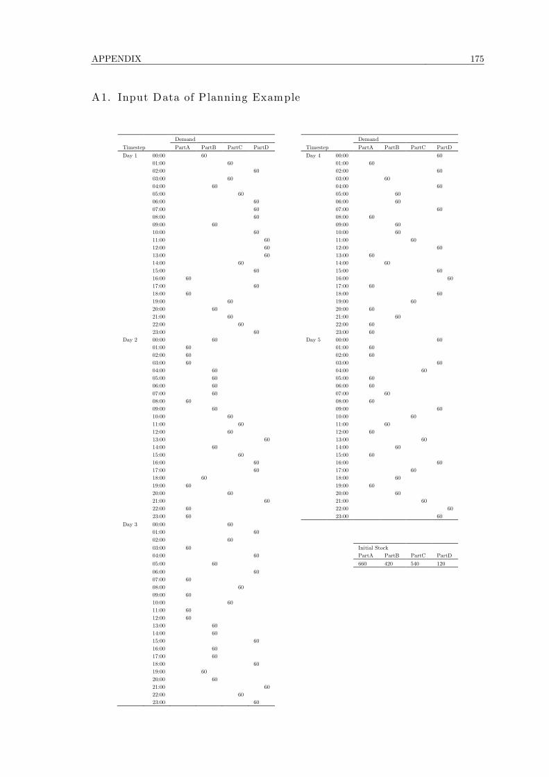
APPENDIX 175
A1. Input Data of Planning Example
Demand Demand
Timestep PartA PartB PartC PartD Timestep PartA PartB PartC PartD
Day 1 00:00 60 Day 4 00:00 60
01:00 60 01:00 60
02:00 60 02:00 60
03:00 60 03:00 60
04:00 60 04:00 60
05:00 60 05:00 60
06:00 60 06:00 60
07:00 60 07:00 60
08:00 60 08:00 60
09:00 60 09:00 60
10:00 60 10:00 60
11:00 60 11:00 60
12:00 60 12:00 60
13:00 60 13:00 60
14:00 60 14:00 60
15:00 60 15:00 60
16:00 60 16:00 60
17:00 60 17:00 60
18:00 60 18:00 60
19:00 60 19:00 60
20:00 60 20:00 60
21:00 60 21:00 60
22:00 60 22:00 60
23:00 60 23:00 60
Day 2 00:00 60 Day 5 00:00 60
01:00 60 01:00 60
02:00 60 02:00 60
03:00 60 03:00 60
04:00 60 04:00 60
05:00 60 05:00 60
06:00 60 06:00 60
07:00 60 07:00 60
08:00 60 08:00 60
09:00 60 09:00 60
10:00 60 10:00 60
11:00 60 11:00 60
12:00 60 12:00 60
13:00 60 13:00 60
14:00 60 14:00 60
15:00 60 15:00 60
16:00 60 16:00 60
17:00 60 17:00 60
18:00 60 18:00 60
19:00 60 19:00 60
20:00 60 20:00 60
21:00 60 21:00 60
22:00 60 22:00 60
23:00 60 23:00 60
Day 3 00:00 60
01:00 60
02:00 60
03:00 60 Initial Stock
04:00 60 PartA PartB PartC PartD
05:00 60 660 420 540 120
06:00 60
07:00 60
08:00 60
09:00 60
10:00 60
11:00 60
12:00 60
13:00 60
14:00 60
15:00 60
16:00 60
17:00 60
18:00 60
19:00 60
20:00 60
21:00 60
22:00 60
23:00 60
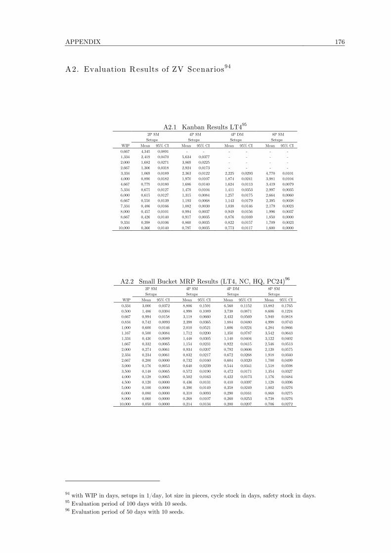
APPENDIX 176
A2. Evaluation Results of ZV Scenarios94
A2.1 Kanban Results LT495
2P SM 4P SM 4P DM 8P SM
Setups Setups Setups Setups
WIP Mean 95% CI Mean 95% CI Mean 95% CI Mean 95% CI
0,667 4,345 0,0891 - - - - - -
1,334 2,419 0,0470 5,634 0,0377 - - - -
2,000 1,682 0,0271 3,869 0,0225 - - - -
2,667 1,306 0,0318 2,924 0,0173 - - - -
3,334 1,069 0,0189 2,363 0,0122 2,225 0,0293 4,770 0,0101
4,000 0,890 0,0182 1,970 0,0107 1,874 0,0241 3,981 0,0104
4,667 0,779 0,0180 1,686 0,0140 1,624 0,0113 3,419 0,0079
5,334 0,675 0,0127 1,479 0,0104 1,411 0,0353 2,997 0,0035
6,000 0,615 0,0127 1,315 0,0084 1,257 0,0175 2,664 0,0060
6,667 0,550 0,0139 1,193 0,0068 1,143 0,0179 2,395 0,0038
7,334 0,486 0,0166 1,082 0,0030 1,038 0,0146 2,179 0,0023
8,000 0,457 0,0101 0,994 0,0037 0,949 0,0156 1,996 0,0037
8,667 0,426 0,0140 0,917 0,0035 0,876 0,0169 1,850 0,0000
9,334 0,398 0,0106 0,860 0,0035 0,822 0,0157 1,709 0,0023
10,000 0,366 0,0140 0,797 0,0035 0,773 0,0117 1,600 0,0000
A2.2 Small Bucket MRP Results (LT4, NC, HQ, PC24)96
2P SM 4P SM 4P DM 8P SM
Setups Setups Setups Setups
WIP Mean 95% CI Mean 95% CI Mean 95% CI Mean 95% CI
0,334 3,000 0,0372 8,806 0,1591 6,560 0,1152 13,882 0,1765
0,500 1,486 0,0304 4,998 0,1089 3,738 0,0871 8,606 0,1224
0,667 0,994 0,0158 3,118 0,0660 2,432 0,0569 5,940 0,0818
0,834 0,742 0,0093 2,398 0,0365 1,884 0,0480 4,998 0,0743
1,000 0,600 0,0146 2,010 0,0521 1,606 0,0224 4,284 0,0866
1,167 0,500 0,0084 1,712 0,0200 1,350 0,0787 3,542 0,0643
1,334 0,430 0,0089 1,448 0,0305 1,140 0,0404 3,122 0,0402
1,667 0,332 0,0065 1,154 0,0231 0,922 0,0415 2,546 0,0513
2,000 0,274 0,0061 0,934 0,0207 0,792 0,0606 2,120 0,0575
2,334 0,234 0,0061 0,832 0,0217 0,672 0,0268 1,918 0,0340
2,667 0,200 0,0000 0,732 0,0160 0,604 0,0320 1,700 0,0499
3,000 0,176 0,0053 0,640 0,0239 0,544 0,0341 1,518 0,0598
3,500 0,148 0,0065 0,572 0,0190 0,472 0,0171 1,354 0,0327
4,000 0,128 0,0065 0,502 0,0163 0,422 0,0173 1,176 0,0484
4,500 0,120 0,0000 0,436 0,0131 0,410 0,0397 1,128 0,0396
5,000 0,100 0,0000 0,390 0,0149 0,358 0,0249 1,002 0,0276
6,000 0,080 0,0000 0,318 0,0093 0,290 0,0161 0,868 0,0275
8,000 0,060 0,0000 0,268 0,0107 0,260 0,0253 0,738 0,0276
10,000 0,050 0,0000 0,214 0,0134 0,200 0,0207 0,706 0,0272
94 with WIP in days, setups in 1/day, lot size in pieces, cycle stock in days, safety stock in days. 95 Evaluation period of 100 days with 10 seeds. 96 Evaluation period of 50 days with 10 seeds.
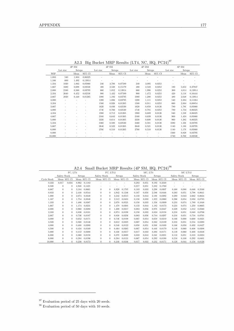
APPENDIX 177
A2.3 Big Bucket MRP Results (LT4, NC, HQ, PC24)97
2P SM 4P SM 4P DM 8P SM
Lot size Setups Lot size Setups Lot size Setups Lot size Setups
WIP Mean 95% CI Mean 95% CI Mean 95% CI Mean 95% CI
1,083 540 1,804 0,06325 - - - - - - - - -
1,166 600 1,492 0,13914 - - - - - - - - -
1,334 1020 1,062 0,05060 240 3,700 0,07589 240 3,095 0,0253 - - -
1,667 1680 0,698 0,02530 480 2,538 0,15179 480 2,522 0,0253 180 5,652 0,37947
2,000 2160 0,560 0,03795 660 1,852 0,13914 660 1,998 0,0253 300 4,014 0,13914
2,334 2640 0,452 0,02530 900 1,432 0,07589 900 1,472 0,0253 420 3,116 0,16444
2,667 2820 0,440 0,01265 1080 1,192 0,03795 1080 1,200 0,0253 480 2,648 0,13914
3,000 - - - 1200 1,086 0,03795 1200 1,111 0,0253 540 2,384 0,11384
3,334 - - - 1500 0,926 0,01265 1500 0,911 0,0253 660 2,004 0,08854
3,667 - - - 1620 0,836 0,02530 1620 0,859 0,0126 780 1,780 0,05060
4,000 - - - 1740 0,766 0,02530 1740 0,781 0,0253 780 1,734 0,06325
4,334 - - - 1980 0,712 0,01265 1980 0,689 0,0126 840 1,538 0,06325
4,667 - - - 2160 0,642 0,01265 2160 0,639 0,0126 900 1,424 0,05060
5,000 - - - 2220 0,614 0,01265 2220 0,608 0,0126 960 1,382 0,06325
5,334 - - - 2460 0,580 0,02530 2460 0,581 0,0126 1080 1,230 0,03795
5,667 - - - 2640 0,522 0,01265 2640 0,521 0,0126 1140 1,180 0,03795
6,000 - - - 2760 0,510 0,01265 2760 0,510 0,0126 1140 1,176 0,05060
8,000 - - - - - - - - - 1560 0,828 0,03795
10,000 - - - - - - - - - 1740 0,768 0,02530
A2.4 Small Bucket MRP Results (4P SM, HQ, PC24)98
FC, LT4 FC, LT12 MC, LT4 MC LT12
Safety Stock Setups Safety Stock Setups Safety Stock Setups Safety Stock Setups
Cycle Stock Mean 95% CI Mean 95% CI Mean 95% CI Mean 95% CI Mean 95% CI Mean 95% CI Mean 95% CI Mean 95% CI
0,333 0,017 0,034 8,962 0,1183 - - - - 0,283 0,051 9,192 0,3348 - - - -
0,500 0 0 4,948 0,1421 - - - - 0,217 0,051 5,232 0,1760 - - - -
0,667 0 0 3,184 0,0661 0 0 8,928 0,1705 0,183 0,033 3,298 0,0307 0,488 0,088 6,646 0,3168
0,833 0 0 2,448 0,0544 0 0 4,942 0,1246 0,167 0,050 2,586 0,0446 0,383 0,051 3,798 0,0641
1,000 0 0 2,074 0,0348 0 0 3,242 0,0515 0,133 0,044 2,180 0,0292 0,293 0,043 2,662 0,0624
1,167 0 0 1,754 0,0348 0 0 2,512 0,0431 0,150 0,033 1,822 0,0360 0,266 0,054 2,050 0,0785
1,333 0 0 1,486 0,0387 0 0 2,078 0,0521 0,150 0,033 1,556 0,0309 0,231 0,074 1,780 0,1048
1,667 0 0 1,174 0,0231 0 0 1,478 0,0301 0,133 0,044 1,182 0,0173 0,231 0,074 1,250 0,0665
2,000 0 0 0,960 0,0280 0 0 1,208 0,0217 0,083 0,056 0,976 0,0347 0,229 0,052 1,012 0,0560
2,333 0 0 0,830 0,0181 0 0 0,974 0,0198 0,150 0,033 0,834 0,0158 0,216 0,051 0,840 0,0706
2,667 0 0 0,736 0,0187 0 0 0,838 0,0256 0,083 0,056 0,744 0,0297 0,216 0,051 0,734 0,0761
3,000 0 0 0,652 0,0171 0 0 0,746 0,0198 0,067 0,054 0,658 0,0219 0,166 0,000 0,600 0,0321
3,500 0 0 0,560 0,0146 0 0 0,612 0,0225 0,067 0,054 0,562 0,0139 0,216 0,051 0,554 0,0280
4,000 0 0 0,488 0,0200 0 0 0,548 0,0122 0,050 0,051 0,500 0,0169 0,166 0,050 0,492 0,0427
4,500 0 0 0,434 0,0169 0 0 0,464 0,0265 0,067 0,054 0,440 0,0179 0,149 0,060 0,408 0,0208
5,000 0 0 0,412 0,0200 0 0 0,430 0,0217 0,017 0,033 0,392 0,0171 0,149 0,060 0,400 0,0348
6,000 0 0 0,360 0,0158 0 0 0,370 0,0089 0,033 0,044 0,340 0,0231 0,116 0,051 0,318 0,0324
8,000 0 0 0,284 0,0196 0 0 0,284 0,0131 0,067 0,054 0,292 0,0190 0,216 0,100 0,292 0,0401
10,000 0 0 0,238 0,0173 0 0 0,240 0,0246 0,017 0,033 0,232 0,0171 0,129 0,044 0,158 0,0126
97 Evaluation period of 25 days with 20 seeds. 98 Evaluation period of 50 days with 10 seeds.
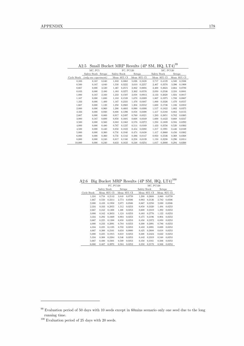
APPENDIX 178
A2.5 Small Bucket MRP Results (4P SM, HQ, LT4)99
MC, PC1 FC, PC120 MC, PC120
Safety Stock Setups Safety Stock Setups Safety Stock Setups
Cycle Stock (only one experiment) Mean 95% CI Mean 95% CI Mean 95% CI Mean 95% CI
0,333 0,167 8,840 1,833 0,3063 5,026 0,2420 2,717 0,4129 4,580 0,2336
0,500 0,167 4,840 1,550 0,3222 3,610 0,2257 2,467 0,3576 3,396 0,1909
0,667 0,000 3,520 1,467 0,2572 2,862 0,0694 2,400 0,3624 2,664 0,0793
0,833 0,000 2,480 1,483 0,3275 2,362 0,0576 2,050 0,2536 2,334 0,0881
1,000 0,167 2,160 1,233 0,1507 2,058 0,0913 2,133 0,2620 1,924 0,0817
1,167 0,000 1,680 1,183 0,1528 1,678 0,0389 1,867 0,1975 1,708 0,0867
1,333 0,000 1,400 1,167 0,2331 1,476 0,0487 1,800 0,3326 1,470 0,0557
1,667 0,000 1,120 1,250 0,2865 1,204 0,0552 1,600 0,1736 1,186 0,0353
2,000 0,000 0,960 1,200 0,4603 0,990 0,0300 1,517 0,1822 1,002 0,0375
2,333 0,000 0,920 0,800 0,1296 0,858 0,0398 1,417 0,2180 0,864 0,0155
2,667 0,000 0,800 0,917 0,2497 0,760 0,0321 1,283 0,3851 0,762 0,0365
3,000 0,167 0,600 0,850 0,1681 0,668 0,0349 1,600 0,4422 0,668 0,0247
3,500 0,000 0,560 0,883 0,1863 0,576 0,0272 1,250 0,1809 0,594 0,0292
4,000 0,000 0,480 0,767 0,1237 0,514 0,0169 1,433 0,3556 0,520 0,0363
4,500 0,000 0,440 0,850 0,1822 0,454 0,0280 1,217 0,1991 0,446 0,0169
5,000 0,000 0,360 0,750 0,1940 0,474 0,0438 1,417 0,3660 0,456 0,0362
6,000 0,000 0,360 0,750 0,1242 0,386 0,0147 0,950 0,2536 0,368 0,0268
8,000 0,000 0,240 0,817 0,1160 0,258 0,0139 1,150 0,3238 0,296 0,0314
10,000 0,000 0,240 0,633 0,1633 0,248 0,0254 1,017 0,3000 0,294 0,0260
A2.6 Big Bucket MRP Results (4P SM, HQ, LT4)100
FC, PC120 MC, PC120
Safety Stock Setups Safety Stock Setups
Cycle Stock Mean 95% CI Mean 95% CI Mean 95% CI Mean 95% CI
1,334 0,758 0,2143 3,848 0,0759 1,208 0,2688 3,860 0,0759
1,667 0,550 0,2214 2,774 0,0506 0,983 0,2126 2,782 0,0506
2,000 0,433 0,1950 2,072 0,0506 0,867 0,3250 2,030 0,0506
2,334 0,333 0,2055 1,512 0,0253 0,858 0,3320 1,494 0,0253
2,667 0,242 0,1300 1,300 0,0253 0,608 0,2319 1,292 0,0253
3,000 0,342 0,2653 1,124 0,0253 0,483 0,2776 1,122 0,0253
3,334 0,292 0,1669 0,904 0,0253 0,475 0,2196 0,904 0,0253
3,667 0,225 0,1388 0,858 0,0253 0,450 0,2372 0,850 0,0253
4,000 0,233 0,2091 0,784 0,0253 0,308 0,2091 0,786 0,0253
4,334 0,225 0,1195 0,702 0,0253 0,433 0,2091 0,698 0,0253
4,667 0,300 0,2161 0,634 0,0000 0,425 0,2688 0,618 0,0253
5,000 0,225 0,1915 0,618 0,0253 0,300 0,2424 0,622 0,0253
5,334 0,308 0,2284 0,546 0,0253 0,442 0,2319 0,548 0,0253
5,667 0,400 0,2301 0,508 0,0253 0,450 0,2161 0,506 0,0253
6,000 0,467 0,3970 0,504 0,0253 0,358 0,2178 0,506 0,0253
99 Evaluation period of 50 days with 10 seeds except in 60mins scenario only one seed due to the long
running time. 100 Evaluation period of 25 days with 20 seeds.
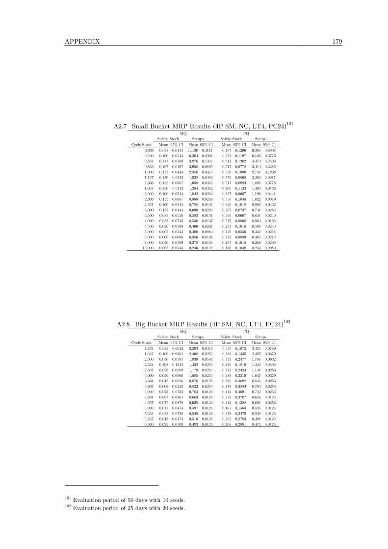
APPENDIX 179
A2.7 Small Bucket MRP Results (4P SM, NC, LT4, PC24)101
MQ PQ
Safety Stock Setups Safety Stock Setups
Cycle Stock Mean 95% CI Mean 95% CI Mean 95% CI Mean 95% CI
0,333 0,033 0,0444 11,130 0,4111 0,467 0,1296 9,366 0,6908
0,500 0,100 0,0544 6,304 0,2381 0,533 0,1197 6,166 0,3776
0,667 0,117 0,0509 3,976 0,1340 0,517 0,1262 4,474 0,2509
0,833 0,167 0,0497 2,958 0,0805 0,517 0,0778 3,414 0,2286
1,000 0,133 0,0444 2,350 0,0470 0,550 0,1000 2,788 0,1238
1,167 0,150 0,0333 1,938 0,0482 0,550 0,0868 2,262 0,0911
1,333 0,133 0,0667 1,688 0,0359 0,517 0,0923 1,892 0,0778
1,667 0,150 0,0333 1,284 0,0352 0,400 0,1133 1,494 0,0733
2,000 0,100 0,0544 1,042 0,0234 0,367 0,0667 1,196 0,0441
2,333 0,133 0,0667 0,888 0,0268 0,350 0,1048 1,022 0,0379
2,667 0,100 0,0544 0,788 0,0136 0,330 0,1018 0,902 0,0432
3,000 0,133 0,0444 0,690 0,0209 0,267 0,0737 0,746 0,0286
3,500 0,083 0,0556 0,582 0,0151 0,300 0,0667 0,630 0,0240
4,000 0,083 0,0745 0,530 0,0137 0,217 0,0868 0,564 0,0196
4,500 0,050 0,0509 0,466 0,0207 0,233 0,1018 0,508 0,0240
5,000 0,067 0,0544 0,400 0,0084 0,250 0,0556 0,442 0,0256
6,000 0,000 0,0000 0,356 0,0131 0,233 0,0889 0,362 0,0219
8,000 0,050 0,0509 0,278 0,0139 0,267 0,1018 0,288 0,0200
10,000 0,067 0,0544 0,246 0,0158 0,150 0,1048 0,244 0,0080
A2.8 Big Bucket MRP Results (4P SM, NC, LT4, PC24)102
MQ PQ
Safety Stock Setups Safety Stock Setups
Cycle Stock Mean 95% CI Mean 95% CI Mean 95% CI Mean 95% CI
1,334 0,083 0,0632 3,293 0,0379 0,350 0,1072 3,435 0,0759
1,667 0,100 0,0861 2,468 0,0253 0,283 0,1335 2,355 0,0379
2,000 0,050 0,0597 1,939 0,0506 0,433 0,2477 1,788 0,0632
2,334 0,108 0,1335 1,432 0,0253 0,450 0,1810 1,343 0,0506
2,667 0,025 0,0509 1,179 0,0253 0,283 0,2424 1,148 0,0253
3,000 0,050 0,0966 1,085 0,0253 0,283 0,2319 1,047 0,0379
3,334 0,042 0,0826 0,876 0,0126 0,508 0,3092 0,843 0,0253
3,667 0,008 0,0228 0,822 0,0253 0,475 0,3883 0,793 0,0253
4,000 0,025 0,0703 0,763 0,0126 0,442 0,4691 0,743 0,0253
4,334 0,067 0,0861 0,663 0,0126 0,358 0,3707 0,656 0,0126
4,667 0,075 0,0878 0,625 0,0126 0,242 0,1388 0,601 0,0253
5,000 0,017 0,0474 0,597 0,0126 0,167 0,1564 0,595 0,0126
5,334 0,033 0,0738 0,545 0,0126 0,358 0,3479 0,538 0,0126
5,667 0,042 0,0474 0,510 0,0126 0,367 0,2793 0,498 0,0126
6,000 0,025 0,0509 0,493 0,0126 0,208 0,2881 0,479 0,0126
101 Evaluation period of 50 days with 10 seeds. 102 Evaluation period of 25 days with 20 seeds.
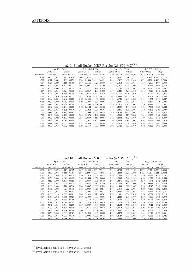
APPENDIX 180
A2.9 Small Bucket MRP Results (2P SM, MC)103
MQ, LT4, PC24 PQ, LT12, PC24 MQ, LT4, PC120 PQ, LT12, PC120
Safety Stock Setups Safety Stock Setups Safety Stock Setups Safety Stock Setups
Cycle Stock Mean 95% CI Mean 95% CI Mean 95% CI Mean 95% CI Mean 95% CI Mean 95% CI Mean 95% CI Mean 95% CI
0,333 0,092 0,0167 4,132 0,1849 0,608 0,0788 9,440 0,7752 1,183 0,2731 2,718 0,3144 1,742 0,2859 6,250 1,1778
0,500 0,117 0,0369 1,736 0,0572 0,700 0,1343 6,420 0,6499 1,000 0,2422 1,432 0,0918 1,583 0,2733 5,410 0,7843
0,667 0,175 0,0389 1,114 0,0130 0,717 0,1144 4,026 0,3586 0,875 0,1454 1,000 0,0711 1,425 0,2158 4,064 0,9861
0,833 0,150 0,0333 0,802 0,0117 0,692 0,0931 2,694 0,3190 0,842 0,1415 0,796 0,0265 1,467 0,3851 2,656 0,7193
1,000 0,150 0,0333 0,638 0,0174 0,617 0,1117 1,744 0,2315 0,917 0,2108 0,592 0,0261 1,433 0,3919 1,700 0,4512
1,167 0,133 0,0444 0,528 0,0186 0,583 0,0657 1,198 0,1303 0,758 0,1348 0,528 0,0148 1,542 0,5020 1,388 0,5268
1,333 0,125 0,0373 0,444 0,0125 0,492 0,0764 0,850 0,1248 0,708 0,1557 0,438 0,0210 1,583 0,3952 0,950 0,2661
1,667 0,150 0,0416 0,348 0,0111 0,417 0,0786 0,530 0,0318 0,667 0,0962 0,350 0,0123 1,825 0,5302 0,612 0,2822
2,000 0,142 0,0434 0,282 0,0090 0,492 0,1500 0,394 0,0236 0,733 0,1736 0,280 0,0133 1,500 0,4574 0,444 0,0371
2,333 0,092 0,0389 0,242 0,0050 0,492 0,1008 0,330 0,0201 0,683 0,2046 0,242 0,0111 1,675 0,6486 0,348 0,0247
2,667 0,083 0,0351 0,204 0,0100 0,392 0,1292 0,258 0,0117 0,450 0,1670 0,210 0,0067 1,708 0,6311 0,272 0,0275
3,000 0,092 0,0524 0,180 0,0000 0,400 0,1133 0,228 0,0133 0,725 0,2898 0,180 0,0060 1,650 0,5962 0,238 0,0324
3,500 0,075 0,0461 0,154 0,0076 0,317 0,1212 0,200 0,0167 0,783 0,2386 0,154 0,0061 1,525 0,4403 0,190 0,0200
4,000 0,083 0,0351 0,136 0,0067 0,375 0,1090 0,204 0,0884 0,650 0,2120 0,130 0,0067 1,375 0,3045 0,154 0,0134
4,500 0,042 0,0278 0,120 0,0000 0,300 0,1575 0,142 0,0050 0,583 0,2950 0,116 0,0053 1,292 0,3125 0,132 0,0088
5,000 0,050 0,0272 0,100 0,0000 0,233 0,0889 0,116 0,0067 0,542 0,2082 0,102 0,0040 1,200 0,7185 0,118 0,0093
6,000 0,033 0,0272 0,082 0,0050 0,233 0,1048 0,100 0,0000 0,200 0,0969 0,086 0,0061 0,950 0,6695 0,096 0,0100
8,000 0,017 0,0222 0,060 0,0000 0,142 0,1026 0,080 0,0105 0,300 0,1614 0,062 0,0040 0,600 0,4680 0,068 0,0065
10,000 0,008 0,0167 0,052 0,0082 0,125 0,1118 0,060 0,0000 0,292 0,1726 0,058 0,0040 0,725 0,8123 0,058 0,0040
A2.10 Small Bucket MRP Results (4P SM, MC)104
MQ, LT4, PC24 PQ, LT12, PC24 MQ, LT4, PC120 PQ, LT12, PC120
Safety Stock Setups Safety Stock Setups Safety Stock Setups Safety Stock Setups
Cycle Stock Mean 95% CI Mean 95% CI Mean 95% CI Mean 95% CI Mean 95% CI Mean 95% CI Mean 95% CI Mean 95% CI
0,333 0,283 0,0711 11,110 0,3127 1,017 0,1822 13,248 0,7241 2,617 0,3753 4,636 0,4292 3,233 0,3855 5,770 1,0956
0,500 0,233 0,0737 6,414 0,1484 1,033 0,2037 10,386 0,7255 2,383 0,4333 3,824 0,3602 3,433 0,5735 5,144 1,0402
0,667 0,200 0,0444 4,096 0,0918 0,950 0,1928 8,084 0,4592 2,150 0,1953 2,980 0,1498 3,467 0,9911 4,116 0,7516
0,833 0,250 0,0556 3,048 0,0489 0,933 0,1333 5,954 0,3060 2,267 0,2906 2,544 0,1492 3,450 0,8059 3,246 0,4339
1,000 0,217 0,0868 2,460 0,0520 0,783 0,0868 4,582 0,3156 1,967 0,3471 2,132 0,1265 3,500 1,0074 2,832 0,3627
1,167 0,200 0,0667 1,996 0,0574 0,833 0,2383 3,612 0,1289 1,850 0,1889 1,852 0,0899 3,300 0,8341 2,542 0,4390
1,333 0,183 0,0598 1,714 0,0723 0,633 0,0667 2,896 0,1594 1,883 0,1495 1,622 0,0907 2,967 0,7647 2,240 0,2649
1,667 0,167 0,0000 1,328 0,0410 0,633 0,0969 2,076 0,0914 1,600 0,1018 1,272 0,0534 3,000 0,8135 1,822 0,3860
2,000 0,167 0,0703 1,086 0,0353 0,583 0,1024 1,600 0,0747 1,533 0,2096 1,056 0,0484 2,850 0,5868 1,376 0,1659
2,333 0,183 0,1160 0,900 0,0231 0,583 0,1024 1,276 0,0751 1,550 0,1991 0,934 0,0413 2,767 0,3031 1,176 0,1142
2,667 0,150 0,0598 0,754 0,0327 0,550 0,1000 1,098 0,0531 1,633 0,2320 0,784 0,0177 2,483 0,4955 0,936 0,0797
3,000 0,167 0,0497 0,686 0,0198 0,483 0,1160 0,920 0,0337 1,517 0,3599 0,702 0,0475 2,400 0,4073 0,892 0,0736
3,500 0,117 0,0711 0,574 0,0189 0,617 0,1410 0,764 0,0495 1,450 0,2813 0,582 0,0350 2,433 0,5515 0,816 0,1330
4,000 0,067 0,0544 0,506 0,0207 0,367 0,0969 0,636 0,0320 1,233 0,2592 0,536 0,0341 2,383 0,5044 0,702 0,0897
4,500 0,100 0,0544 0,474 0,0246 0,367 0,0667 0,536 0,0272 1,733 0,4012 0,506 0,0553 2,033 0,4031 0,592 0,0503
5,000 0,067 0,0544 0,408 0,0208 0,500 0,1111 0,498 0,0411 1,450 0,3687 0,500 0,0382 1,933 0,3692 0,534 0,0405
6,000 0,050 0,0509 0,330 0,0161 0,417 0,1242 0,404 0,0399 1,183 0,2076 0,400 0,0321 1,800 0,4813 0,478 0,0515
8,000 0,067 0,0544 0,268 0,0148 0,333 0,0994 0,278 0,0111 1,000 0,2629 0,250 0,0123 1,833 0,2811 0,310 0,0240
10,000 0,067 0,0544 0,218 0,0151 0,283 0,1495 0,268 0,0268 1,217 0,3222 0,274 0,0260 1,500 0,2854 0,286 0,0547
103 Evaluation period of 50 days with 10 seeds. 104 Evaluation period of 50 days with 10 seeds.
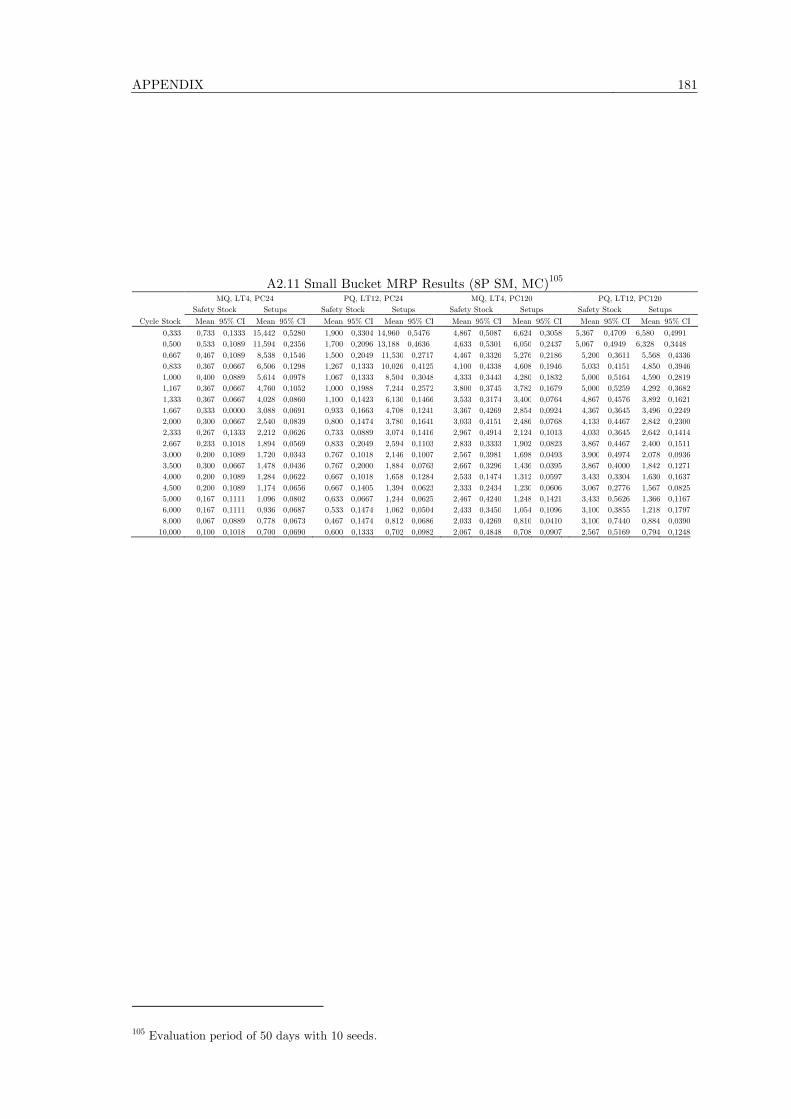
APPENDIX 181
A2.11 Small Bucket MRP Results (8P SM, MC)105
MQ, LT4, PC24 PQ, LT12, PC24 MQ, LT4, PC120 PQ, LT12, PC120
Safety Stock Setups Safety Stock Setups Safety Stock Setups Safety Stock Setups
Cycle Stock Mean 95% CI Mean 95% CI Mean 95% CI Mean 95% CI Mean 95% CI Mean 95% CI Mean 95% CI Mean 95% CI
0,333 0,733 0,1333 15,442 0,5280 1,900 0,3304 14,960 0,5476 4,867 0,5087 6,624 0,3058 5,367 0,4709 6,580 0,4991
0,500 0,533 0,1089 11,594 0,2356 1,700 0,2096 13,188 0,4636 4,633 0,5301 6,050 0,2437 5,067 0,4949 6,328 0,3448
0,667 0,467 0,1089 8,538 0,1546 1,500 0,2049 11,530 0,2717 4,467 0,3326 5,276 0,2186 5,200 0,3611 5,568 0,4336
0,833 0,367 0,0667 6,506 0,1298 1,267 0,1333 10,026 0,4125 4,100 0,4338 4,608 0,1946 5,033 0,4151 4,850 0,3946
1,000 0,400 0,0889 5,614 0,0978 1,067 0,1333 8,504 0,3048 4,333 0,3443 4,280 0,1832 5,000 0,5164 4,590 0,2819
1,167 0,367 0,0667 4,760 0,1052 1,000 0,1988 7,244 0,2572 3,800 0,3745 3,782 0,1679 5,000 0,5259 4,292 0,3682
1,333 0,367 0,0667 4,028 0,0860 1,100 0,1423 6,130 0,1466 3,533 0,3174 3,400 0,0764 4,867 0,4576 3,892 0,1621
1,667 0,333 0,0000 3,088 0,0691 0,933 0,1663 4,708 0,1241 3,367 0,4269 2,854 0,0924 4,367 0,3645 3,496 0,2249
2,000 0,300 0,0667 2,540 0,0839 0,800 0,1474 3,780 0,1641 3,033 0,4151 2,486 0,0768 4,133 0,4467 2,842 0,2300
2,333 0,267 0,1333 2,212 0,0626 0,733 0,0889 3,074 0,1416 2,967 0,4914 2,124 0,1013 4,033 0,3645 2,642 0,1414
2,667 0,233 0,1018 1,894 0,0569 0,833 0,2049 2,594 0,1103 2,833 0,3333 1,902 0,0823 3,867 0,4467 2,400 0,1511
3,000 0,200 0,1089 1,720 0,0343 0,767 0,1018 2,146 0,1007 2,567 0,3981 1,698 0,0493 3,900 0,4974 2,078 0,0936
3,500 0,300 0,0667 1,478 0,0436 0,767 0,2000 1,884 0,0763 2,667 0,3296 1,436 0,0395 3,867 0,4000 1,842 0,1271
4,000 0,200 0,1089 1,284 0,0622 0,667 0,1018 1,658 0,1284 2,533 0,1474 1,312 0,0597 3,433 0,3304 1,630 0,1637
4,500 0,200 0,1089 1,174 0,0656 0,667 0,1405 1,394 0,0623 2,333 0,2434 1,230 0,0606 3,067 0,2776 1,567 0,0825
5,000 0,167 0,1111 1,096 0,0802 0,633 0,0667 1,244 0,0625 2,467 0,4240 1,248 0,1421 3,433 0,5626 1,366 0,1167
6,000 0,167 0,1111 0,936 0,0687 0,533 0,1474 1,062 0,0504 2,433 0,3450 1,054 0,1096 3,100 0,3855 1,218 0,1797
8,000 0,067 0,0889 0,778 0,0673 0,467 0,1474 0,812 0,0686 2,033 0,4269 0,810 0,0410 3,100 0,7440 0,884 0,0390
10,000 0,100 0,1018 0,700 0,0690 0,600 0,1333 0,702 0,0982 2,067 0,4848 0,708 0,0907 2,567 0,5169 0,794 0,1248
105 Evaluation period of 50 days with 10 seeds.
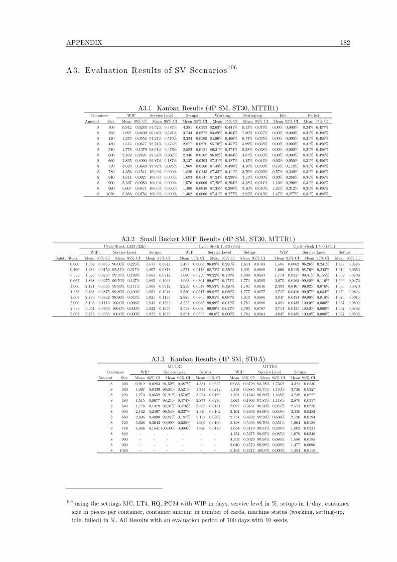
APPENDIX 182
A3. Evaluation Results of SV Scenarios106
A3.1 Kanban Results (4P SM, ST30, MTTR1) Container WIP Service Level Setups Working Setting-up Idle Failed
Amount Size Mean 95% CI Mean 95% CI Mean 95% CI Mean 95% CI Mean 95% CI Mean 95% CI Mean 95% CI
8 300 0,912 0,0283 94,52% 0,487% 4,381 0,0353 82,63% 0,441% 9,13% 0,073% 0,00% 0,000% 8,24% 0,497%
8 360 1,097 0,0439 96,04% 0,521% 3,744 0,0272 83,89% 0,464% 7,80% 0,057% 0,00% 0,000% 8,31% 0,496%
8 420 1,273 0,0552 97,21% 0,570% 3,234 0,0169 84,96% 0,466% 6,74% 0,035% 0,00% 0,000% 8,31% 0,496%
8 480 1,515 0,0677 98,21% 0,474% 2,877 0,0270 85,70% 0,457% 5,99% 0,058% 0,00% 0,000% 8,31% 0,496%
8 540 1,778 0,1379 98,91% 0,476% 2,582 0,0181 86,31% 0,474% 5,38% 0,038% 0,00% 0,000% 8,31% 0,496%
8 600 2,162 0,2497 99,54% 0,337% 2,340 0,0162 86,82% 0,484% 4,87% 0,035% 0,00% 0,000% 8,31% 0,496%
8 660 2,835 0,4090 99,87% 0,187% 2,137 0,0202 87,21% 0,487% 4,45% 0,042% 0,03% 0,050% 8,31% 0,496%
8 720 3,628 0,3643 99,99% 0,028% 1,969 0,0160 87,43% 0,490% 4,10% 0,033% 0,16% 0,118% 8,31% 0,496%
8 780 4,356 0,1541 100,0% 0,000% 1,820 0,0143 87,33% 0,411% 3,79% 0,029% 0,57% 0,240% 8,31% 0,496%
8 840 4,814 0,0927 100,0% 0,000% 1,693 0,0147 87,24% 0,298% 3,53% 0,030% 0,93% 0,268% 8,31% 0,496%
8 900 5,237 0,0980 100,0% 0,000% 1,576 0,0069 87,25% 0,294% 3,28% 0,014% 1,16% 0,299% 8,31% 0,496%
8 960 5,607 0,0871 100,0% 0,000% 1,490 0,0048 87,35% 0,290% 3,10% 0,010% 1,24% 0,312% 8,31% 0,496%
8 1020 5,983 0,0754 100,0% 0,000% 1,402 0,0066 87,31% 0,277% 2,92% 0,013% 1,47% 0,277% 8,31% 0,496%
A3.2 Small Bucket MRP Results (4P SM, ST30, MTTR1) Cycle Stock 1,333 (32h) Cycle Stock 1,416 (34h) Cycle Stock 1,500 (36h)
WIP Service Level Setups WIP Service Level Setups WIP Service Level Setups
Safety Stock Mean 95% CI Mean 95% CI Mean 95% CI Mean 95% CI Mean 95% CI Mean 95% CI Mean 95% CI Mean 95% CI Mean 95% CI
0,000 1,394 0,0055 96,06% 0,225% 1,673 0,0643 1,477 0,0068 96,09% 0,285% 1,613 0,0703 1,585 0,0062 96,26% 0,241% 1,489 0,0496
0,166 1,484 0,0152 98,51% 0,317% 1,807 0,0878 1,571 0,0173 98,72% 0,250% 1,691 0,0688 1,669 0,0119 98,76% 0,243% 1,614 0,0653
0,333 1,586 0,0250 99,37% 0,198% 1,881 0,0812 1,680 0,0230 99,22% 0,159% 1,809 0,0683 1,774 0,0237 99,41% 0,155% 1,689 0,0798
0,667 1,868 0,0275 99,70% 0,137% 1,895 0,1063 1,963 0,0301 99,67% 0,171% 1,771 0,0585 2,075 0,0263 99,80% 0,116% 1,699 0,0473
1,000 2,171 0,0564 99,83% 0,111% 1,898 0,0942 2,259 0,0547 99,83% 0,126% 1,791 0,0646 2,393 0,0407 99,92% 0,076% 1,660 0,0970
1,333 2,468 0,0875 99,89% 0,100% 1,951 0,1248 2,580 0,0517 99,92% 0,089% 1,777 0,0877 2,717 0,0410 99,97% 0,034% 1,659 0,0824
1,667 2,795 0,0862 99,96% 0,044% 1,925 0,1139 2,885 0,0803 99,95% 0,087% 1,813 0,0806 3,047 0,0434 99,99% 0,018% 1,670 0,0915
2,000 3,106 0,1113 100,0% 0,006% 1,941 0,1292 3,225 0,0685 99,99% 0,012% 1,781 0,0898 3,381 0,0435 100,0% 0,000% 1,667 0,0892
2,333 3,451 0,0959 100,0% 0,000% 1,922 0,1059 3,558 0,0690 99,99% 0,013% 1,793 0,0787 3,714 0,0435 100,0% 0,000% 1,667 0,0892
2,667 3,785 0,0959 100,0% 0,000% 1,922 0,1059 3,891 0,0693 100,0% 0,000% 1,784 0,0864 4,047 0,0435 100,0% 0,000% 1,667 0,0892
A3.3 Kanban Results (4P SM, ST0.5) MTTR1 MTTR4
Container WIP Service Level Setups WIP Service Level Setups
Amount Size Mean 95% CI Mean 95% CI Mean 95% CI Mean 95% CI Mean 95% CI Mean 95% CI
8 300 0,912 0,0283 94,52% 0,487% 4,381 0,0353 0,933 0,0729 93,28% 1,734% 4,321 0,0830
8 360 1,097 0,0439 96,04% 0,521% 3,744 0,0272 1,158 0,0885 95,75% 1,150% 3,726 0,0327
8 420 1,273 0,0552 97,21% 0,570% 3,234 0,0169 1,391 0,1540 96,89% 1,168% 3,239 0,0227
8 480 1,515 0,0677 98,21% 0,474% 2,877 0,0270 1,665 0,1906 97,85% 1,118% 2,870 0,0357
8 540 1,778 0,1379 98,91% 0,476% 2,582 0,0181 2,027 0,3657 98,50% 0,957% 2,573 0,0270
8 600 2,162 0,2497 99,54% 0,337% 2,340 0,0162 2,402 0,4469 98,99% 0,848% 2,330 0,0282
8 660 2,835 0,4090 99,87% 0,187% 2,137 0,0202 2,751 0,4832 99,38% 0,636% 2,126 0,0194
8 720 3,628 0,3643 99,99% 0,028% 1,969 0,0160 3,198 0,5330 99,70% 0,351% 1,964 0,0188
8 780 4,356 0,1541 100,00% 0,000% 1,820 0,0143 3,654 0,5119 99,81% 0,234% 1,802 0,0231
8 840 - - - - - - 4,154 0,5275 99,95% 0,085% 1,676 0,0248
8 900 - - - - - - 4,593 0,5029 99,95% 0,086% 1,580 0,0185
8 960 - - - - - - 5,040 0,4570 99,99% 0,028% 1,477 0,0090
8 1020 - - - - - - 5,493 0,4212 100,0% 0,000% 1,394 0,0118
106 using the settings MC, LT4, HQ, PC24 with WIP in days, service level in %, setups in 1/day, container
size in pieces per container, container amount in number of cards, machine status (working, setting-up,
idle, failed) in %. All Results with an evaluation period of 100 days with 10 seeds.
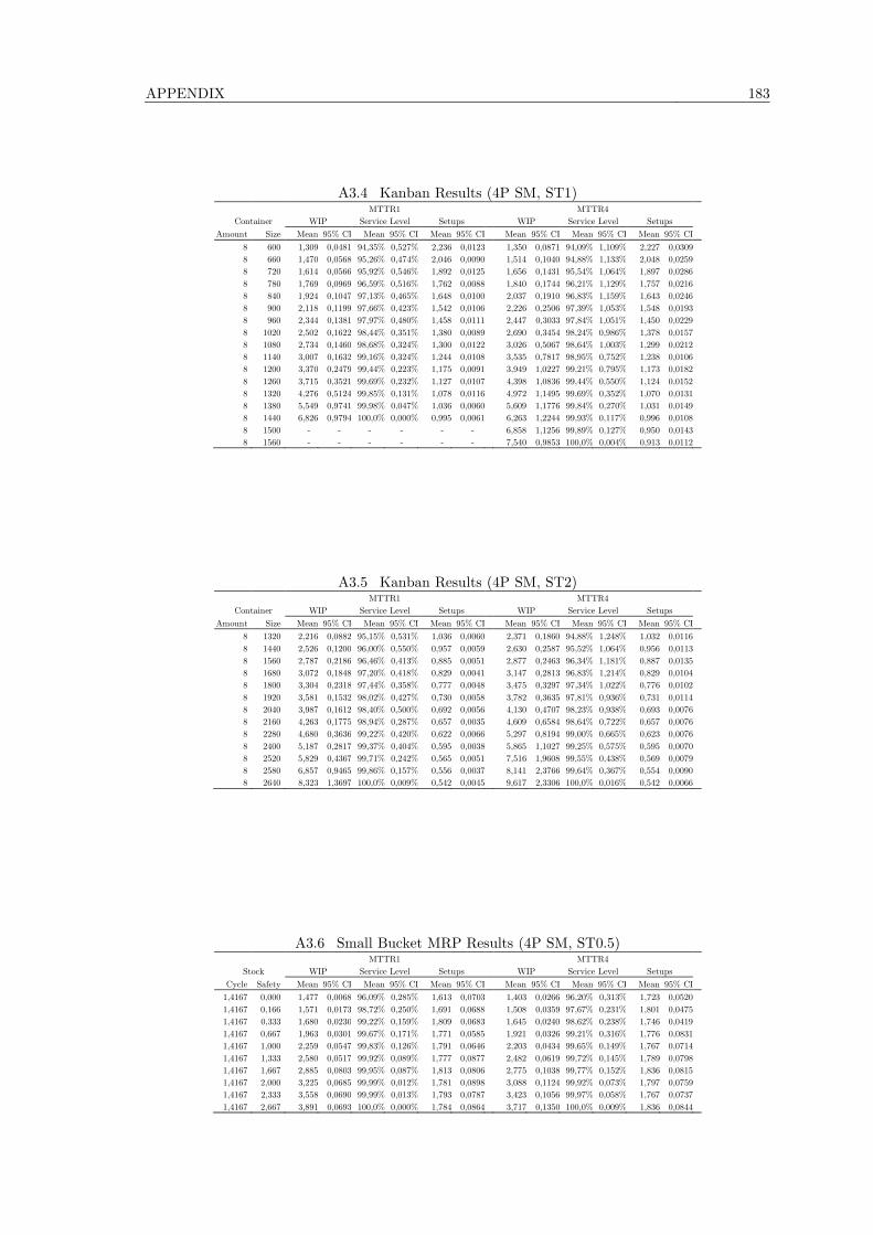
APPENDIX 183
A3.4 Kanban Results (4P SM, ST1) MTTR1 MTTR4
Container WIP Service Level Setups WIP Service Level Setups
Amount Size Mean 95% CI Mean 95% CI Mean 95% CI Mean 95% CI Mean 95% CI Mean 95% CI
8 600 1,309 0,0481 94,35% 0,527% 2,236 0,0123 1,350 0,0871 94,09% 1,109% 2,227 0,0309
8 660 1,470 0,0568 95,26% 0,474% 2,046 0,0090 1,514 0,1040 94,88% 1,133% 2,048 0,0259
8 720 1,614 0,0566 95,92% 0,546% 1,892 0,0125 1,656 0,1431 95,54% 1,064% 1,897 0,0286
8 780 1,769 0,0969 96,59% 0,516% 1,762 0,0088 1,840 0,1744 96,21% 1,129% 1,757 0,0216
8 840 1,924 0,1047 97,13% 0,465% 1,648 0,0100 2,037 0,1910 96,83% 1,159% 1,643 0,0246
8 900 2,118 0,1199 97,66% 0,423% 1,542 0,0106 2,226 0,2506 97,39% 1,053% 1,548 0,0193
8 960 2,344 0,1381 97,97% 0,480% 1,458 0,0111 2,447 0,3033 97,84% 1,051% 1,450 0,0229
8 1020 2,502 0,1622 98,44% 0,351% 1,380 0,0089 2,690 0,3454 98,24% 0,986% 1,378 0,0157
8 1080 2,734 0,1460 98,68% 0,324% 1,300 0,0122 3,026 0,5067 98,64% 1,003% 1,299 0,0212
8 1140 3,007 0,1632 99,16% 0,324% 1,244 0,0108 3,535 0,7817 98,95% 0,752% 1,238 0,0106
8 1200 3,370 0,2479 99,44% 0,223% 1,175 0,0091 3,949 1,0227 99,21% 0,795% 1,173 0,0182
8 1260 3,715 0,3521 99,69% 0,232% 1,127 0,0107 4,398 1,0836 99,44% 0,550% 1,124 0,0152
8 1320 4,276 0,5124 99,85% 0,131% 1,078 0,0116 4,972 1,1495 99,69% 0,352% 1,070 0,0131
8 1380 5,549 0,9741 99,98% 0,047% 1,036 0,0060 5,609 1,1776 99,84% 0,270% 1,031 0,0149
8 1440 6,826 0,9794 100,0% 0,000% 0,995 0,0061 6,263 1,2244 99,93% 0,117% 0,996 0,0108
8 1500 - - - - - - 6,858 1,1256 99,89% 0,127% 0,950 0,0143
8 1560 - - - - - - 7,540 0,9853 100,0% 0,004% 0,913 0,0112
A3.5 Kanban Results (4P SM, ST2) MTTR1 MTTR4
Container WIP Service Level Setups WIP Service Level Setups
Amount Size Mean 95% CI Mean 95% CI Mean 95% CI Mean 95% CI Mean 95% CI Mean 95% CI
8 1320 2,216 0,0882 95,15% 0,531% 1,036 0,0060 2,371 0,1860 94,88% 1,248% 1,032 0,0116
8 1440 2,526 0,1200 96,00% 0,550% 0,957 0,0059 2,630 0,2587 95,52% 1,064% 0,956 0,0113
8 1560 2,787 0,2186 96,46% 0,413% 0,885 0,0051 2,877 0,2463 96,34% 1,181% 0,887 0,0135
8 1680 3,072 0,1848 97,20% 0,418% 0,829 0,0041 3,147 0,2813 96,83% 1,214% 0,829 0,0104
8 1800 3,304 0,2318 97,44% 0,358% 0,777 0,0048 3,475 0,3297 97,34% 1,022% 0,776 0,0102
8 1920 3,581 0,1532 98,02% 0,427% 0,730 0,0058 3,782 0,3635 97,81% 0,936% 0,731 0,0114
8 2040 3,987 0,1612 98,40% 0,500% 0,692 0,0056 4,130 0,4707 98,23% 0,938% 0,693 0,0076
8 2160 4,263 0,1775 98,94% 0,287% 0,657 0,0035 4,609 0,6584 98,64% 0,722% 0,657 0,0076
8 2280 4,680 0,3636 99,22% 0,420% 0,622 0,0066 5,297 0,8194 99,00% 0,665% 0,623 0,0076
8 2400 5,187 0,2817 99,37% 0,404% 0,595 0,0038 5,865 1,1027 99,25% 0,575% 0,595 0,0070
8 2520 5,829 0,4367 99,71% 0,242% 0,565 0,0051 7,516 1,9608 99,55% 0,438% 0,569 0,0079
8 2580 6,857 0,9465 99,86% 0,157% 0,556 0,0037 8,141 2,3766 99,64% 0,367% 0,554 0,0090
8 2640 8,323 1,3697 100,0% 0,009% 0,542 0,0045 9,617 2,3306 100,0% 0,016% 0,542 0,0066
A3.6 Small Bucket MRP Results (4P SM, ST0.5) MTTR1 MTTR4
Stock WIP Service Level Setups WIP Service Level Setups
Cycle Safety Mean 95% CI Mean 95% CI Mean 95% CI Mean 95% CI Mean 95% CI Mean 95% CI
1,4167 0,000 1,477 0,0068 96,09% 0,285% 1,613 0,0703 1,403 0,0266 96,20% 0,313% 1,723 0,0520
1,4167 0,166 1,571 0,0173 98,72% 0,250% 1,691 0,0688 1,508 0,0359 97,67% 0,231% 1,801 0,0475
1,4167 0,333 1,680 0,0230 99,22% 0,159% 1,809 0,0683 1,645 0,0240 98,62% 0,238% 1,746 0,0419
1,4167 0,667 1,963 0,0301 99,67% 0,171% 1,771 0,0585 1,921 0,0326 99,21% 0,316% 1,776 0,0831
1,4167 1,000 2,259 0,0547 99,83% 0,126% 1,791 0,0646 2,203 0,0434 99,65% 0,149% 1,767 0,0714
1,4167 1,333 2,580 0,0517 99,92% 0,089% 1,777 0,0877 2,482 0,0619 99,72% 0,145% 1,789 0,0798
1,4167 1,667 2,885 0,0803 99,95% 0,087% 1,813 0,0806 2,775 0,1038 99,77% 0,152% 1,836 0,0815
1,4167 2,000 3,225 0,0685 99,99% 0,012% 1,781 0,0898 3,088 0,1124 99,92% 0,073% 1,797 0,0759
1,4167 2,333 3,558 0,0690 99,99% 0,013% 1,793 0,0787 3,423 0,1056 99,97% 0,058% 1,767 0,0737
1,4167 2,667 3,891 0,0693 100,0% 0,000% 1,784 0,0864 3,717 0,1350 100,0% 0,009% 1,836 0,0844
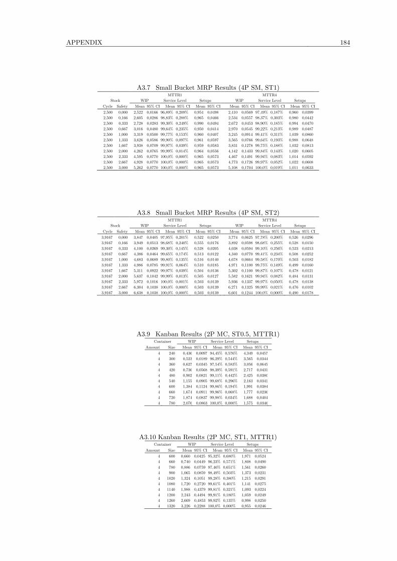
APPENDIX 184
A3.7 Small Bucket MRP Results (4P SM, ST1) MTTR1 MTTR4
Stock WIP Service Level Setups WIP Service Level Setups
Cycle Safety Mean 95% CI Mean 95% CI Mean 95% CI Mean 95% CI Mean 95% CI Mean 95% CI
2,500 0,000 2,522 0,0166 96,89% 0,209% 0,954 0,0498 2,410 0,0569 97,49% 0,187% 0,960 0,0399
2,500 0,166 2,605 0,0286 98,83% 0,288% 0,965 0,0466 2,534 0,0557 98,37% 0,303% 0,980 0,0442
2,500 0,333 2,728 0,0283 99,30% 0,249% 0,990 0,0494 2,672 0,0453 98,90% 0,185% 0,994 0,0470
2,500 0,667 3,016 0,0480 99,64% 0,235% 0,950 0,0414 2,970 0,0545 99,22% 0,213% 0,989 0,0487
2,500 1,000 3,319 0,0500 99,77% 0,153% 0,960 0,0407 3,245 0,0914 99,41% 0,311% 1,039 0,0860
2,500 1,333 3,626 0,0586 99,90% 0,097% 0,961 0,0597 3,565 0,0766 99,64% 0,193% 0,988 0,0648
2,500 1,667 3,938 0,0709 99,97% 0,039% 0,959 0,0583 3,831 0,1278 99,75% 0,188% 1,032 0,0813
2,500 2,000 4,262 0,0765 99,99% 0,014% 0,964 0,0556 4,142 0,1433 99,84% 0,143% 1,020 0,0605
2,500 2,333 4,595 0,0770 100,0% 0,000% 0,965 0,0573 4,467 0,1491 99,94% 0,083% 1,014 0,0592
2,500 2,667 4,928 0,0770 100,0% 0,000% 0,965 0,0573 4,773 0,1726 99,97% 0,052% 1,022 0,0608
2,500 3,000 5,262 0,0770 100,0% 0,000% 0,965 0,0573 5,108 0,1704 100,0% 0,019% 1,011 0,0633
A3.8 Small Bucket MRP Results (4P SM, ST2) MTTR1 MTTR4
Stock WIP Service Level Setups WIP Service Level Setups
Cycle Safety Mean 95% CI Mean 95% CI Mean 95% CI Mean 95% CI Mean 95% CI Mean 95% CI
3,9167 0,000 3,847 0,0405 97,95% 0,201% 0,522 0,0250 3,774 0,0625 97,78% 0,200% 0,526 0,0296
3,9167 0,166 3,949 0,0513 98,68% 0,240% 0,555 0,0176 3,892 0,0598 98,68% 0,255% 0,528 0,0150
3,9167 0,333 4,100 0,0269 99,30% 0,145% 0,528 0,0205 4,038 0,0594 99,10% 0,256% 0,523 0,0213
3,9167 0,667 4,386 0,0464 99,65% 0,174% 0,513 0,0122 4,340 0,0770 99,41% 0,234% 0,508 0,0252
3,9167 1,000 4,683 0,0689 99,80% 0,135% 0,516 0,0140 4,678 0,0664 99,58% 0,170% 0,503 0,0182
3,9167 1,333 4,986 0,0785 99,91% 0,064% 0,510 0,0185 4,971 0,1100 99,75% 0,149% 0,499 0,0160
3,9167 1,667 5,311 0,0922 99,97% 0,039% 0,504 0,0136 5,302 0,1100 99,87% 0,107% 0,478 0,0121
3,9167 2,000 5,637 0,1042 99,99% 0,013% 0,505 0,0127 5,582 0,1621 99,94% 0,082% 0,484 0,0131
3,9167 2,333 5,972 0,1016 100,0% 0,001% 0,503 0,0139 5,936 0,1337 99,97% 0,050% 0,478 0,0138
3,9167 2,667 6,304 0,1038 100,0% 0,000% 0,503 0,0139 6,271 0,1325 99,99% 0,021% 0,476 0,0102
3,9167 3,000 6,638 0,1038 100,0% 0,000% 0,503 0,0139 6,601 0,1244 100,0% 0,000% 0,490 0,0178
A3.9 Kanban Results (2P MC, ST0.5, MTTR1) Container WIP Service Level Setups
Amount Size Mean 95% CI Mean 95% CI Mean 95% CI
4 240 0,436 0,0097 94,45% 0,576% 4,349 0,0457
4 300 0,523 0,0189 96,29% 0,544% 3,565 0,0344
4 360 0,627 0,0345 97,54% 0,583% 3,056 0,0645
4 420 0,736 0,0568 98,39% 0,591% 2,717 0,0431
4 480 0,902 0,0821 99,11% 0,442% 2,425 0,0380
4 540 1,155 0,0905 99,68% 0,296% 2,163 0,0341
4 600 1,384 0,1124 99,86% 0,194% 1,991 0,0384
4 660 1,674 0,0911 99,96% 0,068% 1,777 0,0236
4 720 1,874 0,0837 99,98% 0,034% 1,688 0,0404
4 780 2,076 0,0863 100,0% 0,000% 1,575 0,0346
A3.10 Kanban Results (2P MC, ST1, MTTR1) Container WIP Service Level Setups
Amount Size Mean 95% CI Mean 95% CI Mean 95% CI
4 600 0,660 0,0425 95,32% 0,680% 1,971 0,0524
4 660 0,740 0,0449 96,23% 0,571% 1,808 0,0490
4 780 0,886 0,0759 97,46% 0,651% 1,561 0,0260
4 900 1,065 0,0859 98,49% 0,503% 1,373 0,0231
4 1020 1,324 0,1051 99,28% 0,380% 1,215 0,0291
4 1080 1,720 0,2720 99,61% 0,401% 1,141 0,0275
4 1140 1,988 0,4379 99,81% 0,321% 1,093 0,0224
4 1200 2,243 0,4494 99,91% 0,180% 1,059 0,0249
4 1260 2,669 0,4853 99,92% 0,135% 0,998 0,0250
4 1320 3,226 0,2288 100,0% 0,000% 0,955 0,0246
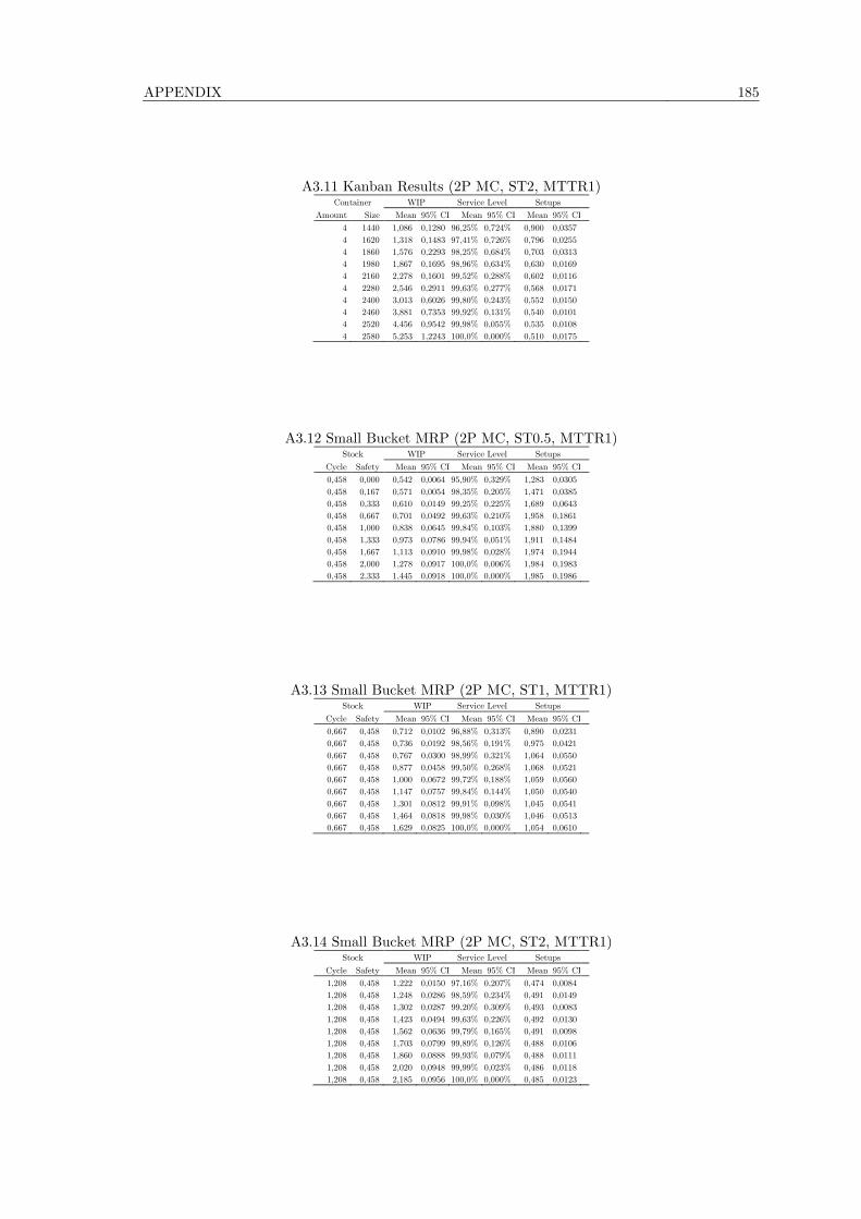
APPENDIX 185
A3.11 Kanban Results (2P MC, ST2, MTTR1) Container WIP Service Level Setups
Amount Size Mean 95% CI Mean 95% CI Mean 95% CI
4 1440 1,086 0,1280 96,25% 0,724% 0,900 0,0357
4 1620 1,318 0,1483 97,41% 0,726% 0,796 0,0255
4 1860 1,576 0,2293 98,25% 0,684% 0,703 0,0313
4 1980 1,867 0,1695 98,96% 0,634% 0,630 0,0169
4 2160 2,278 0,1601 99,52% 0,288% 0,602 0,0116
4 2280 2,546 0,2911 99,63% 0,277% 0,568 0,0171
4 2400 3,013 0,6026 99,80% 0,243% 0,552 0,0150
4 2460 3,881 0,7353 99,92% 0,131% 0,540 0,0101
4 2520 4,456 0,9542 99,98% 0,055% 0,535 0,0108
4 2580 5,253 1,2243 100,0% 0,000% 0,510 0,0175
A3.12 Small Bucket MRP (2P MC, ST0.5, MTTR1) Stock WIP Service Level Setups
Cycle Safety Mean 95% CI Mean 95% CI Mean 95% CI
0,458 0,000 0,542 0,0064 95,90% 0,329% 1,283 0,0305
0,458 0,167 0,571 0,0054 98,35% 0,205% 1,471 0,0385
0,458 0,333 0,610 0,0149 99,25% 0,225% 1,689 0,0643
0,458 0,667 0,701 0,0492 99,63% 0,210% 1,958 0,1861
0,458 1,000 0,838 0,0645 99,84% 0,103% 1,880 0,1399
0,458 1,333 0,973 0,0786 99,94% 0,051% 1,911 0,1484
0,458 1,667 1,113 0,0910 99,98% 0,028% 1,974 0,1944
0,458 2,000 1,278 0,0917 100,0% 0,006% 1,984 0,1983
0,458 2,333 1,445 0,0918 100,0% 0,000% 1,985 0,1986
A3.13 Small Bucket MRP (2P MC, ST1, MTTR1) Stock WIP Service Level Setups
Cycle Safety Mean 95% CI Mean 95% CI Mean 95% CI
0,667 0,458 0,712 0,0102 96,88% 0,313% 0,890 0,0231
0,667 0,458 0,736 0,0192 98,56% 0,191% 0,975 0,0421
0,667 0,458 0,767 0,0300 98,99% 0,321% 1,064 0,0550
0,667 0,458 0,877 0,0458 99,50% 0,268% 1,068 0,0521
0,667 0,458 1,000 0,0672 99,72% 0,188% 1,059 0,0560
0,667 0,458 1,147 0,0757 99,84% 0,144% 1,050 0,0540
0,667 0,458 1,301 0,0812 99,91% 0,098% 1,045 0,0541
0,667 0,458 1,464 0,0818 99,98% 0,030% 1,046 0,0513
0,667 0,458 1,629 0,0825 100,0% 0,000% 1,054 0,0610
A3.14 Small Bucket MRP (2P MC, ST2, MTTR1) Stock WIP Service Level Setups
Cycle Safety Mean 95% CI Mean 95% CI Mean 95% CI
1,208 0,458 1,222 0,0150 97,16% 0,207% 0,474 0,0084
1,208 0,458 1,248 0,0286 98,59% 0,234% 0,491 0,0149
1,208 0,458 1,302 0,0287 99,20% 0,309% 0,493 0,0083
1,208 0,458 1,423 0,0494 99,63% 0,226% 0,492 0,0130
1,208 0,458 1,562 0,0636 99,79% 0,165% 0,491 0,0098
1,208 0,458 1,703 0,0799 99,89% 0,126% 0,488 0,0106
1,208 0,458 1,860 0,0888 99,93% 0,079% 0,488 0,0111
1,208 0,458 2,020 0,0948 99,99% 0,023% 0,486 0,0118
1,208 0,458 2,185 0,0956 100,0% 0,000% 0,485 0,0123
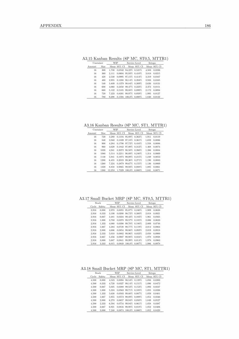
APPENDIX 186
A3.15 Kanban Results (8P MC, ST0,5, MTTR1) Container WIP Service Level Setups
Amount Size Mean 95% CI Mean 95% CI Mean 95% CI
16 300 1,738 0,0532 94,22% 0,531% 4,503 0,0236
16 360 2,111 0,0604 95,93% 0,410% 3,818 0,0215
16 420 2,530 0,0995 97,15% 0,414% 3,319 0,0167
16 480 2,955 0,1288 98,14% 0,394% 2,933 0,0165
16 540 3,409 0,1379 98,84% 0,309% 2,626 0,0131
16 600 4,060 0,2450 99,47% 0,223% 2,373 0,0151
16 660 5,122 0,5185 99,88% 0,099% 2,172 0,0094
16 720 7,223 0,8391 99,97% 0,059% 1,995 0,0127
16 780 9,298 0,1594 100,0% 0,000% 1,840 0,0122
A3.16 Kanban Results (8P MC, ST1, MTTR1) Container WIP Service Level Setups
Amount Size Mean 95% CI Mean 95% CI Mean 95% CI
16 720 3,280 0,1104 95,89% 0,362% 1,911 0,0119
16 840 3,940 0,1339 97,18% 0,361% 1,659 0,0086
16 900 4,284 0,1798 97,72% 0,416% 1,558 0,0088
16 960 4,629 0,1842 97,99% 0,312% 1,468 0,0074
16 1020 4,941 0,2072 98,50% 0,266% 1,386 0,0084
16 1080 5,514 0,2211 98,89% 0,240% 1,314 0,0069
16 1140 5,941 0,1975 99,09% 0,215% 1,249 0,0053
16 1200 6,455 0,2019 99,36% 0,271% 1,190 0,0083
16 1260 7,224 0,3879 99,67% 0,155% 1,136 0,0069
16 1320 8,858 0,9865 99,92% 0,088% 1,085 0,0061
16 1380 12,253 1,7329 100,0% 0,000% 1,041 0,0071
A3.17 Small Bucket MRP (8P MC, ST0,5, MTTR1) Stock WIP Service Level Setups
Cycle Safety Mean 95% CI Mean 95% CI Mean 95% CI
2,916 0,000 2,970 0,0055 95,87% 0,246% 1,909 0,0638
2,916 0,333 3,190 0,0200 98,72% 0,300% 2,018 0,0921
2,916 0,667 3,481 0,0224 99,43% 0,182% 1,961 0,0565
2,916 1,000 3,780 0,0378 99,57% 0,185% 2,006 0,0633
2,916 1,333 4,080 0,0398 99,70% 0,180% 2,009 0,0748
2,916 1,667 4,384 0,0728 99,77% 0,119% 2,014 0,0864
2,916 2,000 4,686 0,0854 99,86% 0,093% 2,019 0,0918
2,916 2,333 5,010 0,0882 99,96% 0,033% 2,050 0,0900
2,916 2,667 5,356 0,0907 99,98% 0,024% 1,978 0,0928
2,916 3,000 5,687 0,0841 99,99% 0,014% 1,978 0,0963
2,916 3,333 6,015 0,0849 100,0% 0,007% 1,986 0,0978
A3.18 Small Bucket MRP (8P MC, ST1, MTTR1) Stock WIP Service Level Setups
Cycle Safety Mean 95% CI Mean 95% CI Mean 95% CI
4,500 0,000 4,523 0,0094 98,54% 0,128% 1,056 0,0200
4,500 0,333 4,720 0,0327 99,14% 0,151% 1,096 0,0472
4,500 0,667 5,025 0,0388 99,52% 0,153% 1,092 0,0247
4,500 1,000 5,324 0,0563 99,71% 0,105% 1,055 0,0326
4,500 1,333 5,638 0,0503 99,80% 0,087% 1,059 0,0401
4,500 1,667 5,955 0,0573 99,89% 0,089% 1,054 0,0346
4,500 2,000 6,270 0,0657 99,94% 0,050% 1,049 0,0527
4,500 2,333 6,594 0,0754 99,94% 0,061% 1,058 0,0387
4,500 2,667 6,921 0,0816 99,98% 0,018% 1,052 0,0406
4,500 3,000 7,248 0,0874 100,0% 0,006% 1,052 0,0420