
Informatica 2 2008 - Babeș-Bolyai University · YEAR Volume 58 (LVIII) 2013 MONTH JUNE ISSUE 2 S T...
129
INFORMATICA 2/2013
Transcript of Informatica 2 2008 - Babeș-Bolyai University · YEAR Volume 58 (LVIII) 2013 MONTH JUNE ISSUE 2 S T...

INFORMATICA2/2013

STUDIA UNIVERSITATIS BABEŞ-BOLYAI
INFORMATICA
No. 2/2013 April - June

This volume contains papers presented at the International Conference KEPT2013
KNOWLEDGE ENGINEERING PRINCIPLES AND TECHNIQUES The conference has been kindly sponsorted by
EDITORIAL BOARD
EDITOR-IN-CHIEF:
Prof. Militon FRENŢIU, Babeş-Bolyai University, Cluj-Napoca, România
EXECUTIVE EDITOR: Prof. Horia F. POP, Babeş-Bolyai University, Cluj-Napoca, România
EDITORIAL BOARD:
Prof. Osei ADJEI, University of Luton, Great Britain Prof. Petru BLAGA, Babeş-Bolyai University, Cluj-Napoca, România Prof. Florian M. BOIAN, Babeş-Bolyai University, Cluj-Napoca, România Assoc.prof. Sergiu CATARANCIUC, State University of Moldova, Chişinău,
Moldova Prof. Gabriela CZIBULA, Babeş-Bolyai University, Cluj-Napoca, România Prof. Dan DUMITRESCU, Babeş-Bolyai University, Cluj-Napoca, România Prof. Farshad FOTOUHI, Wayne State University, Detroit, United States Prof. Zoltán HORVÁTH, Eötvös Loránd University, Budapest, Hungary Prof. Zoltán KÁSA, Babeş-Bolyai University, Cluj-Napoca, România Acad. Solomon MARCUS, Institute of Mathematics, Romanian Academy,
Bucharest Prof. Grigor MOLDOVAN, Babeş-Bolyai University, Cluj-Napoca, România Assoc.prof. Simona MOTOGNA, Babeş-Bolyai University, Cluj-Napoca,
România Prof. Roberto PAIANO, University of Lecce, Italy Prof. Bazil PÂRV, Babeş-Bolyai University, Cluj-Napoca, România Prof. Horia F. POP, Babeş-Bolyai University, Cluj-Napoca, România Prof. Abdel-Badeeh M. SALEM, Ain Shams University, Cairo, Egypt Assoc.prof. Vasile Marian SCUTURICI, INSA de Lyon, France Prof. Doina TǍTAR, Babeş-Bolyai University, Cluj-Napoca, România Prof. Leon ŢÂMBULEA, Babeş-Bolyai University, Cluj-Napoca, România

YEAR Volume 58 (LVIII) 2013 MONTH JUNE ISSUE 2
S T U D I A UNIVERSITATIS BABEŞ-BOLYAI
INFORMATICA
2
EDITORIAL OFFICE: M. Kogălniceanu 1 • 400084 Cluj-Napoca • Tel: 0264.405300
SUMAR – CONTENTS – SOMMAIRE M. Frenţiu, H.F. Pop, S. Motogna, KEPT 2013: The Fourth International Conference On Knowledge Engineering, Principles and Techniques ................................................ 5 INVITED LECTURES A. Adamkó, L. Kollár, Different approaches to MDWE: bridging the gap .................... 9 T. Kozsik, A. Lörincz, D. Juhász, L. Domoszlai, D. Horpácsi, M. Tóth, Z. Horváth, Workflow Description in Cyber-Physical Systems ........................................................ 20 D. Inkpen, A. H. Razavi, Text Representation and General Topic Annotation based On Latent Dirichlet Allocation ...................................................................................... 31 KNOWLEDGE IN COMPUTATIONAL LINGUISTICS D. Tătar, M. Lupea, E. Kapetanios, Hrebs and Cohesion Chains as Similar Tools for Semantic Text Properties Research ............................................................................... 40 A. Varga, A. E. Cano, F. Ciravegna, Y. He, On the Study of Reducing the Lexical Differences Between Social Knowledge Sources and Twitter for Topic Classification . 53 KNOWLEDGE PROCESSING AND DISCOVERY A. Andreica, C. Chira, Weighted Majority Rule for Hybrid Cellular Automata Topology and Neighborhood ......................................................................................... 65

A. Andreica, L. Dio�an, R. D. G�ceanu, A. Sîrbu, ����������� ������������������������� �������� ........................................................................................................ 77
G. Czibula, I. G. Czibula, M. I. Bocicor, �������������������� ������������������������������������ ���������������������� ............................................ 90
D. Chince�, I. Salomie, �!��������� ��������������"��������� ��#�� � ......... 103
N. Gaskó, M. Suciu, R. I. Lung, T. D. Mihoc, D. Dumitrescu, �������$�������%�� �������&���'�()"��!��#��������*���+&��!����������� � ................... 115
T. D. Mihoc, R. I. Lung, D. Dumitrescu, ����!������(������������,������t...123

STUDIA UNIV. BABES–BOLYAI, INFORMATICA, Volume LVIII, Number 2, 2013
KEPT2013: THE FOURTH INTERNATIONAL CONFERENCE
ON KNOWLEDGE ENGINEERING, PRINCIPLES AND
TECHNIQUES
MILITON FRENTIU, HORIA F. POP, AND SIMONA MOTOGNA
1. Introduction
The Faculty of Mathematics and Computer Science of the Babes-BolyaiUniversity in Cluj-Napoca is organizing the Fourth International Conferenceon Knowledge Engineering Principles and Techniques (KEPT2013), duringJuly 5–7, 2013. This conference, organized on the platform of KnowledgeEngineering, is a forum for intellectual, academic, scientific and industrial de-bate to promote research and knowledge in this key area, and to facilitateinterdisciplinary and multidisciplinary approaches, more and more necessaryand useful today. Knowledge engineering refers to the building, maintaining,and development of knowledge-based systems. It has a great deal in commonwith software engineering, and is related to many computer science domainssuch as artificial intelligence, databases, data mining, expert systems, decisionsupport systems and geographic information systems. Knowledge engineeringis also related to mathematical logic, as well as strongly involved in cognitivescience and socio-cognitive engineering where the knowledge is produced bysocio-cognitive aggregates (mainly humans) and is structured according to ourunderstanding of how human reasoning and logic works. Since the mid-1980s,knowledge engineers have developed a number of principles, methods and toolsthat have considerably improved the process of knowledge acquisition and or-dering. Some of the key issues include: there are different types of knowledge,and the right approach and technique should be used for the knowledge understudy; there are different types of experts and ex- pertise, and methods shouldbe chosen appropriately; there are different ways of representing knowledge,which can aid knowledge acquisition, validation and re-use; there are differentways of using knowledge, and the acquisition process can be goal-oriented;there are structured methods to increase the acquisition eficiency.
5

6 MILITON FRENTIU, HORIA F. POP, AND SIMONA MOTOGNA
2. The content of KEPT2013
The Submissions were grouped into four traditional tracks in order tosimplify the review process and Conference presentations. These sections aredescribed downwards.
2.1. Knowledge in Computational Linguistics (KCL). The huge quan-tity of unstructured text documents stored on the web represents issues ofthe very hot researches in Computational Linguistics (or Natural LanguageProcessing, NLP). As a part of Knowledge Engineering, Knowledge in Com-putational Linguistics includes the studies in Linguistic tools in Informationretrieval and Information Extraction, in Text mining, Text entailment andText summarization. The study of Discourse and Dialogue, of Machine learn-ing for natural languages and of Linguistic components of information systemsare also some very active fields in the present research. All these aspects oftheoretical and application-oriented subjects related to NLP are subjects ofdebates in our section of Knowledge in Computational Linguistics.
2.2. Knowledge Processing and Discovery (KPD). The purpose of thistrack is to promote research in AI and scientific exchange among AI re-searchers, practitioners, scientists, and engineers in related disciplines. Topicsinclude but are not limited to the following: Agent-based and multiagentsystems; Cognitive modeling and human interaction; Commonsense reason-ing; Computer vision; Computational Game Theory; Constraint satisfaction,search, and optimization; Game playing and interactive entertainment; Infor-mation retrieval, integration, and extraction; Knowledge acquisition and on-tologies; Knowledge representation and reasoning; Learning models; Machinelearning and data mining; Modelbased systems; Multidisciplinary AI; Naturalcomputing: evolutionary computing, neural computing, DNA and membranecomputing, etc.; Natural language processing; Planning and scheduling; Prob-abilistic reasoning; Robotics; Web and information systems.
2.3. Knowledge in Software Engineering (KSE). The main theme ofthis track is the interplay between software engineering and knowledge engi-neering, answering questions like: how knowledge engineering methods can beapplied to software, knowledge-based systems, software and knowledge-waremaintenance and evolution, applications of knowledge engineering in variousdomains of interest.
2.4. Knowledge in Distributed Computing (KDC). For distributed com-puting and distributed systems, topics of interest include, but are not limitedto, the following: System Architectures for Parallel Computing (including:

KEPT2013: THE FOURTH INTERNATIONAL CONFERENCE 7
Cluster Computing, Grid and Cloud Computing); Distributed Computing (in-cluding: Cooperative and Collaborative Computing, Peer-to-peer Comput-ing, Mobile and Ubiquitous Computing, Web Services and Internet Comput-ing); Distributed Systems (including Distributed Systems Methodology andNetworking, Software Agents and Multi-agent Systems, Distributed SoftwareComponents); Development of Basic Support Components (including Oper-ating Systems for Distributed Systems, Middleware, Algorithms, Models andFormal Verification); Security in Parallel and Distributed Systems.
3. Invited lectures and accepted papers of KEPT2013
This fourth KEPT conference is honored by leading class keynote speakers,to present their invited lectures in two plenary sessions. This year, the lecturesare presented by: Prof. Diana Inkpen (University of Ottawa, Canada), witha lecture on “Text Representation and General Topic Annotation based onLatent Dirichlet Allocation”; Prof. Prof. Attila Adamko (University of De-brecen, Hungary), with a lecture on “Different approaches to MDWE: bridg-ing the gap”; Prof. Zoltan Horvath (Eotvos Lorand University, Budapest,Hungary), with a lecture on “Workflow Description in Cyber-Physical Sys-tems”. The organisation of this conference reflects the following major areasof concern: Natural Language Processing, Knowledge Processing and Discov-ery, Software Engineering, and Knowledge in Distributed Computing. The 18accepted papers (from 29 submitted) were organized in these four sections (2to NLP, 8 to KPD, 3 to SE, and 5 to KDC). The participants submitted theirworks as peer-reviewed papers of 10–12 pages each. These full papers are pub-lished in this and the next issues, 2/2013 and 3/2013, of Studia UniversitatisBabes-Bolyai, Informatica journal.
4. Satellite workshops
Associated to the fourth KEPT conference, we organized three satelliteworkshops. Two of these workshops were organized in colaboration with part-ner companies, offering the opportunity to exchange ideas between academiaand industry. The workshop on “Mobile development”, organized in coopera-tion with the company Skobbler, took place on Friday, July 5, and the work-shop on “Testing methodologies”, organized in cooperation with the companyEndava, took place on Saturday, July 6. As well, for the first time, we orga-nized a satellite doctoral workshop, as an excellent opportunity for doctoralstudents to share their progress on doctoral work, exchange ideas, benefit fromexpert feed-back and defend their research reports.

8 MILITON FRENTIU, HORIA F. POP, AND SIMONA MOTOGNA
5. Conclusions
We hope the Fourth International Conference on Knowledge EngineeringPrinciples and Techniques (KEPT 2013) to be an exciting and useful experi-ence and exchange of knowledge for our department. The possibility to com-municate our most recent studies, and to compare with the results of othercolleagues, the emulation of new ideas and research, all these mean a greatgain of experience in our professional life. We hope that the next editionof KEPT (in 2015) will be even more successful and more enthusiastic thanthis one. We are taking the feedback of this Conference to improve the nexteditions, to atract more participants and to involve more personalities in thereviewing process.
Babes-Bolyai University, Department of Computer Science, Cluj-Napoca,Romania
E-mail address: [email protected]
E-mail address: [email protected]
E-mail address: [email protected]
STUDIA UNIV. BABES–BOLYAI, INFORMATICA, Volume LVIII, Number 2, 2013
DIFFERENT APPROACHES TO MDWE: BRIDGING THE
GAP
ATTILA ADAMKO AND LAJOS KOLLAR
Abstract. This paper will give a short overview and comparison of Model-driven Web Engineering (MDWE) practices applied in both academy andindustry with the aim of bridging the gap between those approaches. WhileDomain Specific Languages (DSLs) are used to express a high level outlineof the imagined systems, the industrial approaches are focusing on a lowerlevel and the distance of the two fields are mostly too wide to apply bothin one development process. The goal of this paper is to propose a way tomerge the two sides. DSLs can help to build prototypes in a very rapidmanner. Based on those prototypes, common models can be derived thatcan serve as a basis for model-driven generation of Web applications usingwell-known production frameworks.
1. Introduction
Model-driven engineering has become more than a promising way of cre-ating applications that are based on abstractions: MDE brings software devel-opment much closer to domain experts. It is the way how the MDA and MDDfield could find its way to real life scenarios. However, these prominent ideaswithout fully realized key technology features cannot lead the way. Withoutexecutable modelling, meta-modelling, language engineering and proper toolsupport they are no more than interesting and idealistic research directions.
In the beginning of the 21st century there were several promising projectsto support MDD and MDE. Nowadays, after a decade of the born of MDAand supporting technologies the list of possible tools with the mentioned keyfeatures are much more limited, only a few of them remain alive. We can
Received by the editors: June 1, 2013.2010 Mathematics Subject Classification. 68U35, 68M11, 68N99.1998 CR Categories and Descriptors. D.2.2 [Software]: Software Engineering – Design
Tools and Techniques; D.2.10 [Software]: Software Engineering – Design.Key words and phrases. MDWE, Web Applications, Model-driven development, Spring,
Domain-Specific Languages.This paper has been presented at the International Conference KEPT2013: Knowledge
Engineering Principles and Techniques, organized by Babes-Bolyai University, Cluj-Napoca,July 5-7 2013.
9

10 A. ADAMKO AND L. KOLLAR
observe a landscape shift from general purpose languages to domain-specificones. It opens the way for bridging the gap between stakeholders, domainexperts and software developers.
2. Domain-specific languages and modeling
In software engineering, a domain-specific language (DSL) is a “a com-puter programming language of limited expressiveness focused on a particulardomain” [6]. A DSL can be either a visual language, like the languages usedby the Eclipse Modeling Framework, or textual languages.
A sound language description contains an abstract syntax, one or moreconcrete syntax descriptions, mappings between abstract and concrete syn-taxes, and a description of the semantics. The abstract syntax of a languageis often defined using a metamodel. The semantics can also be defined usinga metamodel, but in most cases in practice the semantics are not explicitlydefined but they have to be derived from the runtime behavior.
In model-driven engineering, many examples of domain-specific languagesmay be found, like OCL, a language for decorating models with assertions andconstraints, or QVT, a domain-specific model transformation language. How-ever, languages like UML are typically general purpose modeling languages.
Domain-specific languages have important design goals that contrast withthose of general-purpose languages:
• domain-specific languages are less comprehensive;• domain-specific languages are much more expressive in their domain;• domain-specific languages should exhibit minimum redundancy.
3. Academical practices to MDWE
Modeling and systematic design methods are important and emergingfields in the Academic sector. Several new methodologies had born from thisdirection and resulted better software development practices. However, appli-cation of those methodologies are very time-consuming therefore it is mostlyunacceptable for the industry. Several years are required before an approachbecomes a well-functioning method that is ready for industrial use. The fol-lowing sections describe some of the most interesting model-driven languagesand methodologies (without attempting to be comprehensive). (The first oneis an odd one out because it has both academic and industrial aspects.)
3.1. WebML, WebRatio. WebML [4] is a visual notation for specifying thecontent, composition, and navigation features of hypertext applications, build-ing on ER and UML. Its not only for visualizing the models rather than a

DIFFERENT APPROACHES TO MDWE: BRIDGING THE GAP 11
methodology for designing complex data-intensive Web applications. It pro-vides graphical, yet formal, specifications, embodied in a complete design pro-cess. Why it is an odd one out in this list that it has a commertial tool whichcan assist by visual design.
WebML enables designers to express the core features of a site at a highlevel, without committing to detailed architectural details. WebML conceptsare associated with an intuitive graphic representation, which can be easilysupported by CASE tools and effectively communicated to the non-technicalmembers of the site development team. The specification of a site in WebMLconsists of four orthogonal perspectives:
• Structural Model• Hypertext Model
– Composition Model– Navigation Model
• Presentation Model• Personalization Model
At first sight the business process modell is missing from the WebML method-ology but its lying inside the composition model and navigation model, jointlynamed as hypertext model. Native BPMN is not supported by the tool, how-ever there is a transformator which can transform a BPMN diagram into theWebML domain enriching the Application model.
Furthermore, WebML has been extended to cover a wider spectrum offront-end interfaces, thus resulting in the Interaction Flow Modeling Language(IFML), adopted as a standard by the Object Management Group (OMG) in2013.
The WebML language started as a research project at Politecnico di Milanoand later tool support has also been added. This software is called WebRatiothat has become an industrial product so it can be considered as a successstory for bridging the gap between academics and industry. In an ideal world,more ideas originating from the academic sector should reach that stage.
3.2. UML-based Web Engineering. UWE [8] applies the MDA pattern tothe Web application domain from the from analysis to the generated imple-mentation. Model transformations play an important role at every stage of thedevelopment process. The main reasons for using the extension mechanismsof the UML instead of a proprietary modelling technique are the acceptanceof the UML in the field of software development and its extensibility withprofiles. The UWE design approach for Web business processes consists ofintroducing specific process classes that are part of a separate process modelwith a defined interface to the navigation model.

12 A. ADAMKO AND L. KOLLAR
Transformations at the platform independent level support the system-atic development of models, like deriving a default presentation model fromthe navigation model. Then transformation rules that depend on a specificplatform are used to translate the platform independent models describing thestructural aspects of the Web application into models for the specific platform.Finally, these platform specific models are transformed to code by model-to-text transformations. Computer aided design using the UWE method ispossible using MagicUWE, a plugin for MagicDraw.
3.3. WebDSL. WebDSL [11] is a domain-specific language for developingdynamic Web applications with a rich data model. The goal of WebDSLis to get rid of the boilerplate code you would have to write when building aJava application and raise the level of abstraction with simple, domain-specificsub-languages that allow a programmer to specify a certain aspect of theapplication and the WebDSL compiler would generate all the implementationcode for that aspect. The main features of WebDSL are: Domain modeling,Presentation, Page-flow, Access control, Data validation, Workflow, Styling,Email.
Initially there were three sub-languages: a data modeling language, a userinterface language and a simple action language to specify logic. WebDSLapplications are translated to Java Web applications, and the code generatoris implemented using Stratego/XT and SDF.
Although WebDSL is mainly a research project, a case study for domain-specific languages in the Web field [7], it can be usuable by anybody with someprogramming experience.
4. Industrial practices
OMG provides a key foundation for Model-Driven Architecture, which uni-fies every step of development and integration from business modeling, througharchitectural and application modeling, to development, deployment, mainte-nance, and evolution. These concepts and directives have served as a basisfor several solutions built by various companies. The only problem with theseartifacts is the complexity. Complexity requires time and deep knowledge butin real life projects this factor is the most limited one. Companies are focus-ing on fast development time and choose frameworks supporting productivityrather than clear but time-consuming analysis phases. However, the followingproducts could be used in an industrial environment because they have beenproven to be working solutions while utilizing the OMG foundations.
4.1. AndroMDA. In short, AndroMDA is an open source MDA frameworkwhich works on UML models and utilizing plugins and components to generate

DIFFERENT APPROACHES TO MDWE: BRIDGING THE GAP 13
source code for a given programming language. Models are stored in XMIformat produced from different CASE-tools. AndroMDA reads models intomemory, making these object models available to its plugins. These pluginsdefine exactly what AndroMDA will and will not generate. Each plugin iscompletely customizable to a project’s specific needs.
It is mostly used by developers working with J2EE technologies and gen-erate code for Hibernate, EJB, Spring and Web Services. AndroMDA allowscustomization of the templates used for code generation, therefore you cangenerate any additional code you want. We have seen AndroMDA in actionand found it very promising in 2010 [1].
Currently, the only problem is its lost update cycle. The home page waslast updated in 2011 and also the sourceforge repository’s main branch seemsto be stopped. However, there is a small sign of life because timestamps onseveral files in the SNAPSHOT branch show fresh (summer 2013) modificationdate. Because it was successfully applied on one of our industrial projects, ithas the potential and possibility to became an alternative way for bridgingthe two world.
4.2. openArchitectureWare (moved to Eclipse Modeling). OpenAr-chitectureWare (oAW) was the second way for MDA around 2009. It was amodular MDA/MDD generator framework supporting arbitrary models andproviding a language family to check and transform models as well as generatecode based on them. OAW had strong support for EMF (Eclipse ModellingFramework) based models but could work with other models (e.g., UML2,XML or simple JavaBeans) too. The main power of oAW was the workflowengine which allowed to define generator/transformation workflows.
OAW was inherited by the Eclipse Modeling Framework and became abasis for it forming one big integrated family—Xpand (and Xtend), MWE(ant-like definition of transformations chains) and Xtext (textual DSL). Itprovides model-to-model and model-to-text transformation languages but theyare not based on standards.
4.3. Acceleo. Acceleo is a pragmatic implementation of the Object Manage-ment Group (OMG) MOF Model to Text Language (MTL) standard. Thecreator was a French company, named Obeo. Nowadays, Acceleo is an Eclipseproject mostly developed in Java and available under the Eclipse Public Li-cence (EPL) provided by the Eclipse Foundation. During the transition, thelanguage used by Acceleo to define a code generator has been changed to usethe new standard from the OMG for model-to-text transformation, MOFM2T.Acceleo is built on top of several key Eclipse technologies like EMF and, sincethe release of Acceleo 3, the Eclipse implementation of OCL (OMG’s standard

14 A. ADAMKO AND L. KOLLAR
language to navigate in models and to define constraints on the elements of amodel). It has a very good tool support for productive coding.
4.4. Spring. One of the most powerful industrial solutions for Java EE appli-cation development is the Spring Framework. It is an open source applicationframework and Inversion of Control (IoC) container for the Java platform.The core features of the Spring Framework can be used by any Java appli-cations, but there are extensions for building web applications on top of theJava EE platform. Although the Spring Framework does not impose any spe-cific programming model, it has become popular in the Java community as analternative to, replacement for, or even addition to the Enterprise JavaBeans(EJB) model. The Spring Framework comprises several modules that providea range of services including Inversion of Control container, Aspect-orientedprogramming, Data access, Transaction management, Model–View–Controllerpattern, Remote access framework, Authentication and authorization, Messag-ing and Testing. These capabilities make it a strong candidate for industrialprojects.
5. Closing the gap
A number of issues why the high majority of the industry is not committedto model-driven development has been identified in [5]. The authors’ findingsinclude that technical innovation does not go hand in hand with making profit;model-driven approaches are still believed to novel which means that theycannot be trusted enough for adoption; and MDD is considered to be heavy-weight, complex and not mature enough to be used in a real-world developmentproject. They also emphasize that “simplicity is a key feature that helps to sella technology”, however, model-driven approaches can hardly be called simple.
Their additional observations are quite similar to those of [3] and [2]: suc-cessful application of model-driven techniques require a different approach towork (and a basic understanding and commitment) from project participants,revolutionary technologies require new forms of organization, tool support stilldoes not reach the required level, etc. A very important observation statesthat “the tools, training, and expectations of professionals under MDE arenot as well developed and established as those under more traditional softwaredevelopment dynamics” [2].
Despite of having some model-driven solutions that has become an indus-trial product (e.g., WebRatio), their range of application cannot be comparedwith those of the well-known and widely used frameworks like Spring.
Therefore, the existing gap between academical and industrial approachescan be filled, on the one hand, by developing better and better tools andteaching more and more people to think in models, or, on the other hand,

DIFFERENT APPROACHES TO MDWE: BRIDGING THE GAP 15
Figure 1. Web store implementation in WebDSL.
it might be filled by establishing model-based solutions which use the wide-spread production frameworks as a target platform. Our work is focusedon that latter field: we propose a new model-driven generator that is ableto generate source code and the necessary configuration files to the Springframework having Hibernate as a persistence framework.
Since domain-specific languages (especially WebDSL) has been proved tobe very effective in rapid prototyping, our starting point in development wasto use it for easily and quickly define the concepts of the domain. This initialimplementation might serve as a basis for building UML models that can laterbe transformed (using a generator developed for that purpose) to Spring. Thereason for having UML models as intermediate artifacts is twofold: this waythe development can be started by creating the appropriate UML modelswhile it allows other DSL-to-UML mappings to be added later, extending thecapabilities of the system this way.
5.1. Demo application—Web store. In order to demonstrate our ideas, abasic implementation for a Web store application has been created [10]. Theproject has been developed primarily for demonstrational purposes so it lacksmuch functionalities that a real web shop should implement.
This demo emphasizes the rapid prototyping capabilities of WebDSL: itis quite straightforward to create a base (but still useable) application in nomore than 1,000 lines of code.
Figure 1 shows the developed application that has been transformed toJava code by the built-in generator included in the WebDSL Eclipse plugin.
5.1.1. WebDSL implementation and problems. The WebDSL implementationcontains cca. 1,000 lines of code. It includes the definition of business enti-ties (Product, User, Order, OrderItem, Cart, etc.), pages and navigation plus

16 A. ADAMKO AND L. KOLLAR
Figure 2. Excerpt of module Entities (middle) and the gen-erated files (left).
some information on layout and access control. The WebDSL generator hasgenerated 948 Java source files which is quite hard to understand and main-tain. Figure 2 shows an excerpt of the module describing the business entitiesand Of course, a model-driven solution is not intended to modify the gener-ated code (since you are required to modify the model and then re-generate),however, in practice, it is sometimes needed.
5.2. WebDSL to UML transformation. DSLs are backed with metamod-els that capture the abstract syntax (i.e., the knowledge of the domain theDSL is aimed at). Based on that metamodel it is straightforward enough totransform the representation onto a model conforming the UML metamodelso due to lack of space we omit the details of the transformation.
5.3. Generation of Spring implementation from UML model. A gen-erator that is able to generate Spring and Hibernate based implementationof a Web application from a stereotyped UML class diagram, has been devel-oped [9]. The generator itself is built on top of Acceleo and is able to provideimplementation for three layers: data layer, data access layer and businesslogic layer. For the data layer, it generates Hibernate entity classes, the dataaccess layer will contain data access objects (DAOs), while the business logiclayer contains POJIs (Plain Old Java Interfaces) for describing the services.

DIFFERENT APPROACHES TO MDWE: BRIDGING THE GAP 17
Figure 3. Stereotypes the generator understands.
Figure 4. The domain model of the simplified Web store.
XML-based configuration files for both Spring and Hibernate are also gener-ated.
The initial implementation of the generator deals only with class diagrams.Stereotypes are used to determine which layer the class belongs to. Figure 3shows the stereotypes that are processed by the generator.
The domain model that has been created is shown in Figure 4. Its classesare stereotyped with <<entity>>.
Figure 5 demonstrates the Shopping Cart page of the generated Springapplication.

18 A. ADAMKO AND L. KOLLAR
Figure 5. The Shopping Cart page of the generated Spring application.
6. Conclusion
For the MDE community, it is very important that new ideas and methodsdeveloped in the academia appear in industrial practice. Without it, model-driven practices will never reach their potential. This is the reason why weneed increasing number of success stories like WebRatio. However, only afew of the proposed academic approaches receive broader attention from theindustry.
In this paper, we gave a short (and, of course, highly incomplete) overviewof the current state of model-driven engineering in academics and industry. Inorder to close the gap, we proposed a solution for generating applications forthe Spring platform which is widely used across the industry. However, thiswork is not finished: by the time of this paper, our system is able to generatean application based on either a WebDSL descripiton or a UML model butgeneration of business logic is still an open question.
References
[1] A. Adamko and C. Bornemissza. Developing Web-Based Applications Using ModelDriven Architecture and Domain Specific Languages. In Proceedings of the 8th Interna-tional Conference on Applied Informatics, pages 287–293, 2010.
[2] J. Aranda, D. Damian, and A. Borici. Transition to model-driven engineering: what isrevolutionary, what remains the same? In Proceedings of the 15th international confer-ence on Model Driven Engineering Languages and Systems, MODELS’12, pages 692–708, Berlin, Heidelberg, 2012. Springer-Verlag.
[3] P. Baker, S. Loh, and F. Weil. Model-driven engineering in a large industrial context— motorola case study. In Proceedings of the 8th international conference onModel Driven Engineering Languages and Systems, MoDELS’05, pages 476–491, Berlin,Heidelberg, 2005. Springer-Verlag.

DIFFERENT APPROACHES TO MDWE: BRIDGING THE GAP 19
[4] S. Ceri, P. Fraternali, A. Bongio, M. Brambilla, S. Comai, and M. Matera. DesigningData-Intensive Web Applications. Morgan Kaufmann Publishers Inc., San Francisco,CA, USA, 2002.
[5] T. Clark and P.-A. Muller. Exploiting model driven technology: a tale of two startups.Softw. Syst. Model., 11(4):481–493, Oct. 2012.
[6] M. Fowler. Domain Specific Languages. Addison-Wesley Professional, 1st edition, 2010.[7] D. M. Groenewegen, Z. Hemel, and E. Visser. Separation of Concerns and Linguistic
Integration in WebDSL. IEEE Software, 27(5):31–37, 2010.[8] N. Koch and A. Kraus. Towards a common metamodel for the development of web
applications. Cueva Lovelle, Juan Manuel (ed.) et al., Web engineering. Internationalconference, ICWE 2003, Oviedo, Spain, July 14-18, 2003. Proceedings. Berlin: Springer.Lect. Notes Comput. Sci. 2722, 497-506 (2003)., 2003.
[9] A. Locsei. Webalkalmazasok modell alapu keszıtese, 2013. Bachelor’s thesis, Universityof Debrecen, Hungary, In Hungarian. Thesis supervisor: Lajos Kollar.
[10] L. Szarka. Modell-Vezerelt Webfejlesztesi Megoldasok. Master’s thesis, University ofDebrecen, Hungary, 2013. In Hungarian. Thesis supervisor: Attila Adamko.
[11] E. Visser. WebDSL: A Case Study in Domain-Specific Language Engineering. InR. Lammel, J. Visser, and J. a. Saraiva, editors, Generative and Transformational Tech-niques in Software Engineering II, pages 291–373. Springer-Verlag, Berlin, Heidelberg,2008.
Department of Information Technology, Faculty of Informatics, Universityof Debrecen, H–4028 Debrecen, Kassai ut 26., Hungary
E-mail address: [email protected]
Department of Information Technology, Faculty of Informatics, Universityof Debrecen, H–4028 Debrecen, Kassai ut 26., Hungary
E-mail address: [email protected]

STUDIA UNIV. BABES–BOLYAI, INFORMATICA, Volume LVIII, Number 2, 2013
WORKFLOW DESCRIPTION
IN CYBER-PHYSICAL SYSTEMS
TAMAS KOZSIK, ANDRAS LORINCZ, DAVID JUHASZ, LASZLO DOMOSZLAI,
DANIEL HORPACSI, MELINDA TOTH, AND ZOLTAN HORVATH
Abstract. Cyber-physical systems (CPS) are networks of computationaland physical processes, often containing human actors. In a CPS-setting,the computational processes collect information on their physical environ-ment via sensors, and react upon via actuators in order to reach a desiredstate of the physical world.
In the approach presented in this paper a CPS application is imple-mented as a hierarchical workflow of mostly independent tasks, which areexecuted in a distributed environment, and satisfy timing constraints. Incertain cases such workflows can be defined from natural language descrip-tions with the use of ontologies. The structure of a workflow, as well asthe constraints put on the constituting tasks, are expressed in a domain-specific programming language.
1. Introduction
There is a growing need for complex controllable distributed systems.Some examples, selected randomly to illustrate the vast diversity of the ap-plication domains, are as follows: automated production lines, public trans-portation with driverless cars, infantry fighting vehicles, robotic surgery andinternet-based multi-player augmented reality games. Cyber-physical systems(CPS) are networks of computational and physical processes, often containing
Received by the editors: June 1, 2013.2010 Mathematics Subject Classification. 68N15, 68M14.1998 CR Categories and Descriptors. D3.2 [Programming Languages]: Language
Classifications – Applicative (functional) languages, Concurrent, distributed, and parallellanguages.
Key words and phrases. cyber-physical system, task-oriented programming, workflow,timing constraint, domain specific language.
This paper has been presented at the International Conference KEPT2013: KnowledgeEngineering Principles and Techniques, organized by Babes-Bolyai University, Cluj-Napoca,July 5-7 2013.
20

WORKFLOW DESCRIPTION IN CYBER-PHYSICAL SYSTEMS 21
human actors. In a CPS-setting, the computational processes collect informa-tion on their physical environment via sensors, and react upon via actuatorsin order to reach a desired state of the physical world.
There is a related emerging challenge for system and software development,which is concerned with the multi-faceted (physical, computational, psycholog-ical, cognitive), multi-layered (mobile, WLAN, backbone), multi-level (micro-to-macro), distributed computation and communication, from RF MEMS tocloud computing.
We suggest a novel route to address the challenge that we call CPS Pro-gramming, and which is concerned with the development of a domain specificlanguage (DSL) for cyber-physical systems. The DSL is capable to describedistributed workflows, the timing constraints of the tasks involved, and fault-tolerance mechanisms.
In this paper, we propose a way for defining the computational parts ofcomplex cyber-physical systems as workflows composed from hierarchical, in-dependent building blocks. We have worked out a workflow system, wherethere are combinators specifically relevant to CPS Programming: time con-straints, distribution, fault-tolerance and error-correction can be easily definedby means of them. We also describe the embedding of a domain-specific work-flow language in Erlang.
The rest of the paper is structured as follows. Section 2 exposes theconcepts for defining cyber-physical systems with workflows. Our workflow-system and its relevance to CPS Programming are revealed in Section 3. Fi-nally, Section 4 concludes the paper.
2. The main concepts
The methodology proposed here splits up an application into modules, eachimplementing an (orchestrated set of) action(s) that can be executed, often ina reactive manner, in parallel with other actions. The main requirement is thatinteraction between modules should be minimized. There are two underlyingreasons behind this constraint. Firstly, if interaction is complex, then timerequirements of testing, as well as bandwidth requirements for real time errorcorrection and reconfiguration will become unbearable. Secondly, unexpectedinstabilities might emerge because of the complexity and the accumulation of(small) errors in a controlled non-linear system.
We note that interaction with an ongoing process is slow, and the mod-ification of a stable trajectory could be hard and may take time. Consider,for example, that in a given moment, say at time t, some deviation α fromplanned behavior is detected. If we were to choose a correction module thatcan correct α, we would ignore that the execution of the correction module
22 KOZSIK, LORINCZ, JUHASZ, DOMOSZLAI, HORPACSI, TOTH, AND HORVATH
begins after a certain delay, the execution itself takes time, and the ongoingprocess may have side-effects on our correction module.
Hence, in order to meet our constraints, the progress of the applicationshould be monitored, and whenever a failure, or some deviation from plannedbehavior is detected, a new correcting (sub)goal must be defined. In otherwords, we notice the deviation, predict its future dynamics, and make a planto minimize the costs in the future on the top of the ongoing process. Wehave made the following assumptions: (i) we have a model, (ii) we can carryout model-based prediction, (iii) we can perform long-term cost optimizationon the top of any ongoing process by means of modules, and (iv) these mod-ules have minimal (or at least tolerable) side-effects on the ongoing process.This way we may (eventually) cope with the unavoidable delays apparent ina distributed and/or concurrent system.
2.1. An illustrative example from nature. Evolution teaches us for therelevance of the cost of interaction [1]. The brain has 1011 neurons, but only1014 connections (instead of 1022). Furthermore, the evolved system is builtfrom robust (and complex) modules, but with minimized side-effects. Con-sider, for example, the mammalian control system [2], which has the followingproperties.
(1) Control space is divided according to high level tasks (eating, grasp-ing, chewing, defense, manipulation in central space, climbing etc.),only a few may be concurrent at a time, but many (low complexity)combinations are executable in parallel.
(2) Each high level task is divided into sub-tasks; e.g., grasping is di-vided according to the discretization of the allo-centric 3D space withinreach. It thus avoids combinatorial explosion of muscle space and isrobust with respect to the huge dimension of body configuration space.
We conclude that module structure should be goal (task) driven and thatthe minimization of side-effects seems mandatory at least for the mammaliandecision making and executive systems.
2.2. Task and Test Driven Development. A specific feature of CPS Pro-gramming is the software development methodology. The methodology mustrespect certain constraints, such as the use of a large number of units, stochas-tic behavior, delays in the execution of modules, system components originat-ing from different sources, and humans-in-the-loop. Moreover, due to depend-ability requirements inherent in the CPS domain, the methodology shouldsupport both testing and verification. The main problem to solve here is theavoidance of combinatorial explosion both in the number of variables, and inthe number of test cases.

WORKFLOW DESCRIPTION IN CYBER-PHYSICAL SYSTEMS 23
The number of basic variables is typically large, and the full space scaleswith the number of variables in the exponent. Even evolution does not havethe time to test all structures against one another in such a huge space. Asopposed to evolution, our design serves certain tasks, so we are to test onlythose structures that have the promise of solving the task.
Note that tasks should be defined by decomposing goals, so they express atop-down approach. Testing, on the other hand, concerns the cases determinedby the existing variables, so it is a bottom-up process. Unless we can limit thenumber of variables stepwise, we cannot test our solutions. This leads us tothe well-known concept of side-effect free concurrent modules: if we test theindividual modules at one level, then they may become our variables (in thesense that we may decide whether to include them) at the next level.
2.3. Implementation aspect. The above mentioned methodology is bestsupported by a domain specific language which is suitable to describe tasks,as well as task hierarchies and related timing constraints. Task-oriented pro-gramming [3] (TOP) provides the right paradigm for this DSL. “In TOP, atask is a specified piece of work aiming to produce a result of known type.When executed, tasks produce (temporary) results that can be observed ina controlled way. As work progresses it can be continuously monitored andcontrolled by other tasks. Tasks can either be fully automated, or can beperformed by humans with computer support.”
Complex workflows involving sensors, actuators, humans and communica-tion in a distributed environment can be expressed as compositions of simplertasks, using predefined and programmer-defined combinators. The DSL canfacilitate the introduction of application-specific combinators in the form ofhigher-order functions. The description of timing constraints should be a cen-tral language feature in the DSL.
The technique of language embedding allows the use of a powerful hostlanguage in the embedded domain specific language. We are to start withErlang; Erlang will be the host language. This choice is motivated by certainErlang features: (i) Erlang is well-suited to programming distributed and con-current systems and even more importantly, (ii) Erlang’s concept of supervisorprocesses enables the easy implementation of fault-tolerance mechanisms.
We describe our framework, which is a good basis for bottom-up definitionof workflows, in Section 3. The aim of a task-oriented programming DSL is toprovide a syntax that resembles to natural language description of workflows,and focuses on the high level structures relevant to domain experts. Sinceits expressive power can lead to the definition of rather complex systems,and thus testing and verification might suffer from this complexity, the use

24 KOZSIK, LORINCZ, JUHASZ, DOMOSZLAI, HORPACSI, TOTH, AND HORVATH
of the Task and Test Driven Development methodology is fostered. The top-down methodology can be improved by connecting with dialogue systems, andmaking the generation of workflows from application domain specific ontologiesand natural language commands feasible.
3. The CPS Workflow System
In this section, a brief informal introduction to our framework is providedas follows. Section 3.1 classifies the entities of our system as special kinds oftasks. Section 3.2 presents a simple example that already utilizes the basiccombinators. Finally, Section 3.3 gives a short description on embedding ourDSL in Erlang.
3.1. Everything is a task. In a workflow system, tasks are first class citizens.This means that tasks can be arguments and results of other tasks, and, sincewe focus on a distributed execution environment, they can even be transmittedover the network. Tasks can be composed using “combinators”, forming morecomplex tasks. In this approach, a complete workflow is a task as well.
Different kinds of tasks can be identified according to their function ina CPS workflow. The differentiation of tasks in our system can be seen inFigure 1.
A task consists of two parts: the description of its behavior, and theconstraints on its execution. The behavior defines the computation the taskperforms when launched. The constraints part of a task specify spatial, timingand resource requirements, such as where to execute the task in a distributedenvironment, or what timeout triggers the cancellation of the task in the caseof some failure.
We can distinguish two kinds of tasks. Primitive tasks are the simplestbuilding blocks of workflows: interaction with a sensor or an actuator is aprimitive task in a cyber-physical system. Moreover, any computation thatis considered atomic according to the problem domain will be defined as aprimitive task.
Combinators are tasks building new tasks from existing ones. They canbe classified into two groups: a constructor combines the computational partsof its arguments, and a specificator establishes the constraints of a task. Moredetails on combinators will be exposed through examples later on.
3.2. Basic combinators. As an illustration, let us consider a simple example,which contains already some of the main concepts of real-world cyber-physicalsystems, albeit in a small scale. We emphasize four issues regarding a CPSproblem here: reading sensors, controlling actuators, operating under specifiedconstraints, and using model-based predictions for correction modules.

WORKFLOW DESCRIPTION IN CYBER-PHYSICAL SYSTEMS 25
TaskComputation
+Constraints
Primitive task Combinator
Read sensorControl actuator
Atomic computationConstructor Specificator
Combining computation
Altering constraints
Build more complex tasks
Figure 1. Everything is a task in a workflow system
In the example we want to bring water to boil in a kettle: we can switch ona coil to heat the water, we can check the water temperature regularly, and wecan switch off the coil when the boiling point is reached. Constraints specifythe location where the boiling water is needed, as well as the deadline when thewater must reach 100oC. Furthermore, we want to bring water to boil fault-tolerantly. For example, if the coil breaks down, we want to switch on anotherone in order to make sure that the water will eventually boil. We have a simplephysical model: the temperature of the water is increasing continuously whenthe coil that heats the water is on. If we observe that this condition is notmet, we conclude that either the coil or the thermometer is broken. By usingmore than one thermometers, and by cumulating sensory data, we can detectbreakage of the thermometer. By using more than one coils, electricity to thebroken coil can be cut off, and another coil can be switched on. A workflowimplementing this functionality is depicted in Figure 2, and the source codeof this workflow is presented in listing kettle.wf.
This workflow must be run a node connected to a kettle. Having the coilswitched on, we start checking the temperature with three thermometers inparallel. We repeatedly read the thermometers, and the stream of sensorydata is channeled to the model. We compute the average of the measuredtemperatures, and check whether the boiling point of water is reached. 97oCis used due to sensor accuracy. The conditional control structure is provided by

26 KOZSIK, LORINCZ, JUHASZ, DOMOSZLAI, HORPACSI, TOTH, AND HORVATH
@!KETTLE
Switch on coil acc ← 0
ts
t > 97 °CAverage tst
Switch off coil
{true}{false}
Read thermometer
Read thermometer
Read thermometer
acc - t > δ
{true}{false}
Set alarm on
acc ← t; t t
ts
Figure 2. Bringing water to boil
the host language our DSL is embedded into. If the boiling point is reached,we switch off the coil, and stop the parallel tasks. If the water is not hotenough, we can compare the temperature against our physical model. If thetemperature has not been raised since the last reading of the thermometers,we trigger an alarm and end the workflow. The state maintained by themodel is “acc” (which stands for accumulator); it contains the previously readtemperature data. Its initial value is 0, and the current temperature is savedinto it at the end of each activation when the workflow is not stopped.
Now consider the building blocks of this simple workflow example. Theprimitive tasks here are the following: read a thermometer, switch on/off acoil and set the alarm. In the graphical representation two special symbolsrepresent the starting and terminating points of the workflow.
What kind of combinators can we observe in this example? First of all,two tasks can be combined sequentially, which means that the second one willbe launched when the first one ends. In some cases the result of the first task

WORKFLOW DESCRIPTION IN CYBER-PHYSICAL SYSTEMS 27
1 −module( k e t t l e ) .
3 −export ( main /0) .
5 main ( ) −>Workflow =
7 k e t t l e c o n t r o l : s e t c o i l ( on ) >>|par ( [ rec ( k e t t l e c o n t r o l : read thermometer ( i ) >>= fun ( t ) −>
9 continue ( t ) end)| i <−[ 1 ,2 ,3 ] ] )
11 controlled by fun ( acc , t s ) −>average ( t s ) >>= fun ( t ) −>
13 i ft > 97 −>
15 k e t t l e c o n t r o l : s e t c o i l ( o f f ) >>|return ( t ) ;
17 acc − t > e r r o r t r e s h o l d −>k e t t l e c o n t r o l : s e t a l a rm ( on ) >>|
19 k e t t l e c o n t r o l : s e t c o i l ( o f f ) >>|return ({ e r ror , t} )
21 true −>continue ({t , t} )
23 endend
25 endwith accumulator 0 @! [ k e t t l e ] ,
27execute ( Workflow ) .
. kettle.wf
is needed by the second. For instance, after computing the average of thevalues supplied by the three thermometers, we pass the result to the decisionmaking task. (This is expressed by the >>= constructor in the DSL, whichbinds the value of the first task to a fresh variable – described as an “explicitfun-expression” in Erlang.) On the other hand, after switching the coil on,we can start reading the thermometers without passing any values from thefirst task to the second one. (This is expressed with the >>| constructor inthe DSL.)
To describe parallel control flow, one can use the par constructor, whichlaunches a number of tasks simultaneously. The compound task ends only if allof its components have ended, and its result is a list of the results of the com-ponents. Reading sensory data from the three thermometers is implementedwith the parallel combinator in our example.

28 KOZSIK, LORINCZ, JUHASZ, DOMOSZLAI, HORPACSI, TOTH, AND HORVATH
Workflows are often described in the style of reactive programming: thestate of a subsystem can be monitored, and the workflow can react on changesof this state. According to our approach, we have a model which can plan anideal trajectory in the problem space, and decide about error correction whendeviation from that trajectory is detected.
Constraints can be associated to tasks, such as the spatial constraint@!KETTLE in the example. The specificator @ can be used to impose require-ments on the location where a task must be executed. In our example, wespecify that the complete workflow must be launched on a node that is an-notated with the “KETTLE” property. Specifying requirements on availableresources as well as on user identities and roles is also possible in this way.
An interesting aspect of the @ combinator is that it ensures implicit codetransfer among nodes of a distributed system. Adaptivity of components in aCPS application and autonomy of tasks are fostered by allowing their code tobe transfered by the workflow runtime in a transparent way. As an additionalconsequence, there is no need to deploy all the components of an applicationon all the nodes of the executing distributed execution environment, a min-imal workflow runtime suffices: the code of the tasks can be transfered bythe runtime to the appropriate node when needed, and hence the distributedexecution environment can dynamically (re-)configure itself.
To make the workflow hierarchical, a special constructor, called a controllerhas been introduced. To understand its semantics, the concept of unstablevalues must be considered first. When a task ends, the value it results willnever change: it is called a “stable value”. In the case of sequences, whena task ends, its result is propagated forwards in the control flow as a stablevalue, but, in addition to this, it is also propagated backwards as an “unstablevalue”. If we have a complex task, it may produce multiple unstable valuesbefore it reaches an end, and provides a stable value: its final result. AsFigure 3 illustrates, the repeated read of a sensor (or any repeated executionof some task) will also yield a stream of unstable values.
Controllers provide a way to work with unstable values. The construct canbe written as “controlled by” in the source code, and it binds a name tothe unstable values observed. A controller has two tasks associated with it: a“controlled task” (of which the unstable values are observed by the controller),and a “plan”. The plan is a task as well, with a very special meaning in theworkflow. When a controller is launched, it launches the observed task. Everyunstable value propagated from the observed task triggers the execution ofthe plan associated to the controller. Plans may maintain a state betweendifferent activations and can decide to stop the controlled task when a desiredgoal is reached, or in the case of faults/failures. Finally, when the controlledtask ends, its stable value is propagated as the result of the controller.

WORKFLOW DESCRIPTION IN CYBER-PHYSICAL SYSTEMS 29
Task1 Task2Read
sensor
Figure 3. Raising unstable values
Note that error detection and correction can be implemented in the planof a controller. Therefore, controllers are the major means for model-basedprediction and decision making in workflows. This is reflected in the kettleexample as well.
3.3. Behind the curtain – How the DSL is implemented. As mentionedalready in Section 2.3, workflow systems are described by using a softwareframework, which is in fact a simple programming language embedded intoErlang. It was a design decision that we implement distributed workflow sys-tems in Erlang, since it is one of the most favored programming languagesfor implementing highly scalable, distributed, reliable and fault-tolerant soft-ware systems. In addition, we prefer this language also because it gives usthe potential of employing the RefactorErl tool for statically analyzing andtransforming the source code.
We chose Erlang despite the fact that it is not extensible, and it is cer-tainly not suitable for DSL embedding. However, we found that the programtransformation capabilities of RefactorErl can be easily turned into programtranslation capabilities; thus, we can extend the Erlang programming lan-guage with some key elements required for effective language embedding. Theframework and the workflows are implemented in an extended version of theErlang language, which is translated back to simple Erlang in one single step.The resulting program is compiled and run as any other Erlang application.
Since Erlang does not allow sending functions among different nodes ofthe network, computations cannot be handed over in an intuitive and effort-less way. We developed support for so-called portable functions, realized as acompile-time transformation, which turns anonymous functions into complexdata terms representing the computations along with their dependencies at-tached. On the other hand, the embedding of domain specific concepts intothe language is mainly supported by the possibility of defining prefix and in-fix operators composed of natural language elements. Beside these two maincomponents, we introduced some pieces of syntactic sugar that result in morenatural workflow descriptions.
30 KOZSIK, LORINCZ, JUHASZ, DOMOSZLAI, HORPACSI, TOTH, AND HORVATH
4. Conclusion
A programming methodology for cyber-physical systems has been pro-posed in this paper. The methodology emphasizes the introduction of moduleswith limited interaction, constraining the concurrent execution of interferingmodules, and the need to avoid combinatorial explosion of test cases for vali-dation.
A domain specific language for describing workflows can facilitate the de-velopment of CPS applications. The main concepts of such a language aretasks, combinators and constraints. In the CPS domain timing constraintsare especially relevant.
We have presented a domain specific workflow language embedded intoErlang. This embedding provides the constructs of a powerful host language,as well as the superior distribution and fault tolerance capabilities of the Erlangprogramming model.
Acknowledgement
The research was carried out as part of the EITKIC 12-1-2012-0001 project,which is supported by the Hungarian Government, managed by the NationalDevelopment Agency, financed by the Research and Technology InnovationFund and was performed in cooperation with the EIT ICT Labs BudapestAssociate Partner Group (www.ictlabs.elte.hu).
References
[1] J. Clune, J.B. Mouret, and H. Lipson. The evolutionary origins of modularity. Proc. R.Soc. B, 280(1755), 2013.
[2] M. S. A. Graziano. The organization of behavioral repertoire in motor cortex. AnnualReview of Neuroscience, 29:105–134, 2006.
[3] B. Lijnse. TOP to the rescue: Task-Oriented Programming for incident response. PhDthesis, Radboud Universiteit Nijmegen, 2013. ISBN 978-90-820259-0-3, IPA DissertationSeries 2013-4.
Faculty of Informatics, Eotvos Lorand University, Budapest, Hungary
STUDIA UNIV. BABES–BOLYAI, INFORMATICA, Volume LVIII, Number 2, 2013
TEXT REPRESENTATION AND GENERAL TOPIC
ANNOTATION BASED ON LATENT DIRICHLET
ALLOCATION
DIANA INKPEN(1) AND AMIR H. RAZAVI(2)
Abstract. We propose a low-dimensional text representation method fortopic classification. A Latent Dirichet Allocation (LDA) model is built ona large amount of unlabelled data, in order to extract potential topic clus-ters. Each document is represented as a distribution over these clusters.We experiment with two datasets. We collected the first dataset from theFriendFeed social network and we manually annotated part of it with 10general classes. The second dataset is a standard text classification bench-mark, Reuters 21578, the R8 subset (annotated with 8 classes). We showthat classification based on the LDA representation leads to acceptableresults, while combining a bag-of-words representation with the LDA rep-resentation leads to further improvements. We also propose a multi-levelLDA representation that catches topic cluster distributions from genericones to more specific ones.
1. Introduction
In order to improve the performance of text classification tasks, we alwaysneed informative and expressive methods to represent the texts [14] [16]. Ifwe consider the words as the smallest informative unit of a text, there is avariety of well-known quantitative information measures that can be used torepresent a text. Such methods have been used in a variety of information
Received by the editors: June 1, 2013.2010 Mathematics Subject Classification. 62Fxx Parametric inference, 62Pxx
Applications.1998 CR Categories and Descriptors. code [I.2.7 Natural Language Processing]:
Subtopic – Text analisys code [H.3.1 Content Analysis and Indexing]: Subtopic –Linguistic processing ;
Key words and phrases. automatic text classification, topic detection, latent Dirichletallocation.
This paper has been presented at the International Conference KEPT2013: KnowledgeEngineering Principles and Techniques, organized by Babes-Bolyai University, Cluj-Napoca,July 5-7 2013.
31
32 INKPEN AND RAZAVI
extraction projects, and in many cases have even outperformed some syntax-based methods. There are a variety of Vector Space Models (VSM) whichhave been well explained and compared, for example in [18]. However, thesekinds of representations disregard valuable knowledge that could be inferredby considering the different types of relations between the words. These majorrelations are actually the essential components that, at a higher level, couldexpress concepts or explain the main topic of a text. A representation methodwhich could add some kind of relations and dependencies to the raw informa-tion items, and illustrate the characteristics of a text at different conceptuallevels, could play an important role in knowledge extraction, concept analysisand sentiment analysis tasks.
In this paper, the main focus is on how we represent the topics of thetexts. Thus, we select a LDA topic-based representation method. We alsoexperiment with a multi-level LDA-based topic representation. Then, we runmachine learning algorithms on each representation (or combinations), in orderto explore the most discriminative representation for the task of text classifi-cation, for the two datasets that we selected.
2. Related work
In the most text classification tasks, the texts are represented as a set ofindependent units such as unigrams / bag of words (BOW), bigrams and/ormulti-grams which construct the feature space, and the text is normally rep-resented only by the assigned values (binary, frequency or term TF-IDF1) [17].In this case, since most lexical features occur only a few times in each con-text, if at all, the representation vectors tend to be very sparse. This methodhas two disadvantages. First, very similar contexts may be represented bydifferent features in the vector space. Second, in short instances, we will havetoo many zero features for machine learning algorithms, including supervisedclassification methods.
Blei, Ng and Jordan proposed the Latent Dirichlet Allocation (LDA)model and a Variational Expectation-Maximization algorithm for trainingtheir model. LDA is a generative probabilistic model of a corpus and theidea behind it is that the documents are represented as weighted relevancyvectors over latent topics, where a topic is characterized by a distribution overwords. These topic models are a kind of hierarchical Bayesian models of acorpus [2]. The model can unveil the main themes of a corpus which can po-tentially be used to organize, search, and explore the documents of the corpus.In LDA models, a topic is a distribution over the feature space of the corpusand each document can be represented by several topics with different weights.
1term frequency / inverse document frequency

TEXT REPRESENTATION AND GENERAL TOPIC ANNOTATION BASED ON LDA 33
The number of topics (clusters) and the proportion of vocabulary that createeach topic (the number of words in a cluster) are considered as two hiddenvariables of the model. The conditional distribution of these variables, givenan observed set of documents, is regarded as the main challenge of the model.
Griffiths and Steyvers in 2004, applied a derivation of the Gibbs samplingalgorithm for learning LDA models [9]. They showed that the extracted topicscapture a meaningful structure of the data. The captured structure is consis-tent with the class labels assigned by the authors of the articles that composedthe dataset. The paper presents further applications of this analysis, such asidentifying hot topics by examining temporal dynamics and tagging some ab-stracts to help exploring the semantic content. Since then, the Gibbs samplingalgorithm was shown as more efficient than other LDA training methods, e.g.,variational EM and Expectation-Propagation [12]. This efficiency is attributedto a famous attribute of LDA namely, ”the conjugacy between the Dirichletdistribution and the multinomial likelihood”. This means that the conjugateprior is useful, since the posterior distribution is the same as the prior, and itmakes inference feasible; therefore, when we are doing sampling, the posteriorsampling become easier. Hence, the Gibbs sampling algorithms was appliedfor inference in a variety of models which extend LDA [19], [7], [4], [3], [11].
Recently, Mimno et al. presented a hybrid algorithm for Bayesian topicmodeling in which the main effort is to combine the efficiency of sparse Gibbssampling with the scalability of online stochastic inference [13]. They usedtheir algorithm to analyze a corpus that included 1.2 million books (33 billionwords) with thousands of topics. They showed that their approach reducesthe bias of variational inference and can be generalized by many Bayesianhidden-variable models.
3. Datasets
The first dataset that we prepared for our experiments consists in threadsfrom the FriendFeed social network. We collected main postings (12,450,658)and their corresponding comments (3,749,890) in order to obtain all the dis-cussion threads (a thread consists in a message and its follow up comments).We filtered out the threads with less than three comments. We were left with24,000 threads. From these, we used 4,000 randomly-selected threads as back-ground source of data, in order to build the LDA model. We randomly selected500 threads and manually annotated them with 10 general classes2, to use astraining and test data for the classification. The 10 classes are: consumers,
2We used only one annotator, but we had a second annotator check a small subset, in orderto validate the quality of annotation. In future work, we plan to have a second annotatorlabel all the 500 threads.

34 INKPEN AND RAZAVI
Class No. of Training Docs No. of Test Docs TotalAcq 1596 696 2292Earn 2840 1083 3923Grain 41 10 51Interest 190 81 271Money-fx 206 87 293Ship 108 36 144Trade 251 75 326Crude 253 121 374Total 5485 2189 7674
Table 1. Class distribution of training and testing data for R8.
education, entertainment, life stories, lifestyle, politics, relationships, religion,science, social life and technology.
The second dataset that we chose for our experiments is the well-known R8subset of the Reuters-21578 collection (excerpted from the UCI machine learn-ing repository), a typical text classification benchmark. The data includes the8 most frequent classes of Reuteres-21578; hence the topics that will be con-sidered as class labels in our experiments are acq, crude, earn, grain, interest,money, ship and trade.
In order to follow the Sebastiani’s convention [16], we also call the datasetR8. Note that there is also a R10 dataset, and the substantial differencebetween R10 and R8 is that the classes corn and wheat, which are closelyrelated to the class grain, were removed. The distribution of documents perclass and the split into training and test data for the R8 subset is shown inTable 1.
4. Method
We trained LDA models for each of the two datasets: one model on 4000threads from FriendFeed and one model on all the R8 text data. LDA modelshave two parameters whose values need to be chosen experimentally: the num-ber of topic clusters and the number of words in each cluster. We experimentedwith various parameter values of the LDA models.
For the first dataset, the best classification results were obtained by settingthe number of cluster topics to 50, and the number of words in each clusterto maximum 15.
In LDA models, polysemous words can be member of more than one topi-cal cluster, while synonymous words are normally gathered in the same topics.An example of LDA topic cluster for the first model is: ”Google”, ”email”,

TEXT REPRESENTATION AND GENERAL TOPIC ANNOTATION BASED ON LDA 35
”search”, ”work”, ”site”, ”services”, ”image”, ”click”, ”page”, ”create”, ”con-tact”, ”connect”, ”buzz”, ”Gmail”, ”mail”. This could be labeled as Internet.
As mentioned, our 500 threads were manually annotated with the 10generic classes. These classes, enumerated in section 3, are a manually gener-alized version of the 50 LDA clusters into the 10 generic categories. For theabove example, the annotator placed it under the technology and social lifecategories. The classification task is therefore multi-class, since a thread canbe in more than one class. We trained binary classifiers from Weka [20] foreach class, and averaged the results over all classes.
The manual mapping of LDA clusters into generic classes would allow usto automatically annotate more training data form the FriendFeed dataset, inour future work. Since each document has LDA clusters that were associatedto it during the Gibbs sampling process, the generic classes for these clusterscan be obtained, and one or more labels can be assigned to the document.Only the labels with high LDA weights will be retained. If the weights are lowfor all labels, the document would not be added to the training data. If morethan one label has high weight, the document would have multiple labels. Thisprocess would allow us to add a large amount of training data, perhaps withsome noise. For more details see [15].
For the classification task, we chose several classifiers from Weka: NaiveBayes (NB) because it is fast and works well with text, SVM since it is knownto obtain high performance on many tasks, and decision trees because we canmanually inspect the learned tree.
We applied these classifies on simple bag-of-words (BOW) representation,on LDA-based representations of different granularities, and on an integratedrepresentation concatenating the BOW features and the LDA features. Thevalues of the LDA-based features for each document are the weights of theclusters associated to the document by the LDA model (probability distribu-tions).
5. Experiments and Results
The results on the first dataset are presented in Table 2. After stop-word removal and stemming, the bag-of-words (BOW) representation con-tained 6573 words as features (TF-IDF values). The lower-dimensional repre-sentation based on LDA contained 50 features, whose values are the weightscorresponding to the topic clusters. For the combined representation (BOWintegrated with the LDA topics) the number of features was 6623.
We observed that the 10 class labels (general topics) are distributed un-evenly over the dataset of 500 threads, in which we had 21 threads for the classconsumers, 10 threads for education, 92 threads for entertainment, 28 threads

36 INKPEN AND RAZAVI
Representation / Classifier AccuracyBOW(TF-IDF)/ CompNB 77.22%LDA Topics / Adaboost (j48) 69.32%BOW(TF-IDF)+LDA / SVM(SMO) 80.00%Table 2. Results on the FriendFeed dataset.
for incidents, 90 threads for lifestyle, 27 threads for politics, 58 threads forrelationships, 31 threads for science, 49 threads for social activities, and 94threads for technology. Thus, the baseline of any classification experimentover this dataset may be considered as 18.8%, for a trivial classifier that putseverything in the most frequent class, technology. However, after balancing theabove distribution through over/under sampling techniques, the classificationbaseline lowered to 10%.
On this dataset, we conducted the classification evaluations using strati-fied 10-fold cross-validations (this means that the classifier is trained on nineparts of the data and tested on the remaining part, then this is repeated 10times for different splits, and the results are averaged over the 10 folds). Weperformed several experiments on a range of classifiers and parameters foreach representation, to check the stability of a classifier’s performance. Wechanged the seed, a randomization parameter of the 10-fold cross-validation,in order to avoid the accidental over-fitting.
For the BOW representation, the best classifier was Complement NaiveBayes (a version of NB that compensates for data imbalance), with an accu-racy of 77.22%. Using the low-dimensional LDA representation, the accuracygoes down, but it has the advantage that the classifiers are faster and otherclassifiers could be used (that do not usually run on high-dimensional data).Combining the two representations achieved the best results, 80% accuracy.
The results on the second dataset, R8, are shown in Table 3. We experi-mented with several parameters for the LDA model: 8, 16, 32, 64, 128, and 256for the number of clusters (therefore we build 6 models). We chose 20 words ineach cluster. The reason we started with 8 clusters is that there are 8 classesin the annotated data. We experimented with combinations of the models inthe feature representation (a multi-leveal LDA-based representation), leavingup to the classifier to choose an appropriate level of generalization.
After stopword removal and stemming, the BOW representation (TF-IDFvalues) contained 17387 words as the feature space. We experimented witheach LDA representation separately, without good results; therefore we chosea combined 6-level representation (corresponding to the LDA models with 256,128, 64, 32, 16, 8 clusters). For the integrated representation BOW with LDA

TEXT REPRESENTATION AND GENERAL TOPIC ANNOTATION BASED ON LDA 37
Representation / Classifier AccuracyBOW / SVM 93.33%LDA Topics / SVM 95.89%LDA+BOW / SVM 97.03%BOW / NB 95.20%LDA Topics / NB 94.61%LDA+BOW / NB 95.52%BOW / DT 91.54%LDA Topics / DT 91.78%Table 3. Results on the R8 dataset.
topics we had 17891 features (256 + 128 + 64 + 32 + 16 + 8 = 504, plus the17387 words).
The average classification accuracy is very high, compared to a baselineof 51% (of a simplistic 8-way classifier that always chooses the most frequentclass, earn in this dataset). The SVM and NB classifiers achieved the bestresults. These values are in line with state-of-the art results reports in the lit-erature. We can compare our results with other reported classification resultsof the same dataset. According to the best of our knowledge, the accuracyof our integrated representation method on the Reuters R8 dataset, 97%, ishigher than any simple and combinatory representation method from relatedwork, which reports accuracies of 88%–95% [6], [1], [5], while 96% was reachedwith SVM on a complex representation method based on kernel functions andLatent Semantic Indexing [21].
For SVM, the LDA-based representation achieved better accuracy (95.89%)than the BOW representation (93.33%). This is due to the multi-level repre-sentation. When we experimented with each level separately, the accuraciesdropped considerably. The best results over all the experiments were for SVMwith the combined BOW and LDA-based representation.
6. Conclusions and Future Work
As our experimental results show, we can achieve good classification resultsby using a low-dimensional representation based on LDA. This representationhas the advantage that allows the use of classifiers or clustering algorithmsthat cannot run on high-dimensional feature spaces. By using a multi-levelrepresentation (different generalization levels) we achieved better results thanthe BOW representation on the second dataset. In future work, we plan to testthe multi-level representation on the first dataset, to confirm our hypothesisthat it is better to let classifiers choose the appropriate level of generalization.

38 INKPEN AND RAZAVI
The combined BOW and LDA features representation achieved the bestclassification performance, and it can be used when there memory is not aconcern, for classifiers that are able to cope with the large vector spaces.
Our results show that the first dataset is more difficult to classify than thesecond dataset. The reason is that it consists in social media texts, which arevery noisy. In future work, we plan to experiment with more training datafor the FriendFeed dataset (automatically annotated via the mapping of LDAclusters into the 10 classes), and to design representation and classificationmethods that are more appropriate for this kind of data.
Acknowledgments
The authors wish to thank Ontario Centres of Excellence and to The Nat-ural Sciences and Engineering Research Council of Canada for the financialsupport. We thank Lana Bogouslavski for annotating the FriendFeed dataand Dmitry Brusilovsky for his insights in the project.
References
[1] Charu C. Aggarwal and Peixiang Zhao. 2012. Towards graphical models for text pro-cessing; Knowledge Information Systems, DOI 10.1007/s10115-012-0552-3; Springer-VerlagLondon.
[2] David M. Blei, T. L. Griffiths, M. I. Jordan, and J. B. Tenenbaum. Hierarchical topicmodels and the nested Chinese restaurant process. In Proceedings of the conference onNeutral Processing Information Systems NIPS 2003.
[3] David M. Blei and J. McAulie. 2007. Supervised topic models. In Proceedings of theconference on Neutral Processing Information Systems NIPS 2007.
[4] David M. Blei, Andrew Ng, and Michael Jordan. Latent Dirichlet Allocation. 2003. Jour-nal of Machine Learning Research, 3: 993–1022.
[5] Ana Cardoso-Cachopo, Arlindo L. Oliveira. 2007. Combining LSI with other Classifiers toImprove Accuracy of Single-label Text Categorization. In Proceedings of the first EuropeanWorkshop on Latent Semantic Analysis in Technology Enhanced Learning, EWLSATEL2007.
[6] Yen-Liang Chen and Tung-Lin Yu. 2011. News Classification based on experts’ workknowledge. In Proceedings of the 2nd International Conference on Networking and Infor-mation Technology IPCSIT 2011, vol.17 ; IACSIT Press, Singapore.
[7] Andrew McCallum and X. Wang. 2005. Topic and role discovery in social networks. InProceedings of IJCAI 2005.
[8] J. R. Firth et al. 1957. Studies in Linguistic Analysis. A synopsis of linguistic theory,1930–1955. Special volume of the Philological Society. Oxford: Blackwell.
[9] Thomas L. Griffiths and Mark Steyvers. 2004. Finding scientific topics. In Proceedingsof the National Academy of Sciences, 101 (Suppl 1), 5228–5235.
[10] Gregor Heinrich. 2004. Parameter estimation for text analysis, Technical Re-port (For further information please refer to JGibbLDA at the following link:http://jgibblda.sourceforge.net/)
[11] Wei Li and Andrew McCallum. 2006. Pachinko allocation: Dag-structured mixturemodels of topic correlations. In Proceedings of ICML 2006.

TEXT REPRESENTATION AND GENERAL TOPIC ANNOTATION BASED ON LDA 39
[12] Thomas Minka and John Lafferty. 2002. Expectation propagation for the generative as-pect model. In Proceedings of the 18th Annual Conference on Uncertainty in Artificial Intel-ligence UAI 2002. https://research.microsoft.com/minka/papers/aspect/minka-aspect.pdf.
[13] David Mimno, M. Hoffman, and David M. Blei. 2012. Sparse stochastic inference forlatent Dirichlet allocation. In Proceedings of International Conference on Machine LearningICML 2012.
[14] Xiaoshan Pan and Hisham Assal. 2003. Providing context for free text interpretation.In Proceedings of Natural Language Processing and Knowledge Engineering, 704–709.
[15] Amir H. Razavi and Diana Inkpen. 2013. General Topic Annotation in Social Networks:A Latent Dirichlet Allocation Approach. In Proceedings of the 26th Canadian Conferenceon Artificial Intelligence (AI 2013), Regina, SK, Canada.
[16] Fabrizio Sebastiani. 2006. Classification of text, automatic. In Keith Brown (ed.), TheEncyclopedia of Language and Linguistics, Volume 14, 2nd Edition, Elsevier Science Pub-lishers, Amsterdam, NL, 457–462.
[17] Karin Spark Jones. 1972. A statistical interpretation of term specificity and its applica-tion in retrieval. Journal of Documentation 28 (1): 11–21.
[18] Peter D. Turney and Patrick Pantel. 2010. From frequency to meaning: Vector spacemodels of semantics, Journal of Artificial Intelligence Research (JAIR), 37, 141–188.
[19] Xuerui Wang and Andrew McCallum. 2006. Topics over time: A non-Markovcontinuous-time model of topical trends. In Proceedings of ACM SIGKDD conference onKnowledge Discovery and Data Mining KDD 2006.
[20] Ian H. Witten and Eibe Frank. 2005. Data Mining: Practical Machine Learning Toolsand Techniques, 2nd edition, Morgan Kaufmann, San Francisco.
[21] Man Yuan, Yuan Xin Ouyang and Zhang Xiong. 2013. A Text Categorization Methodusing Extended Vector Space Model by Frequent Term Sets. Journal of Information Scienceand Engineering 29, 99–114.
(1) University of Ottawa, School of Electrical Engineering and ComputerScience, Ottawa, ON, Canada, K1N 6N5
E-mail address: [email protected]
(2) University of Ottawa, School of Electrical Engineering and ComputerScience, Ottawa, ON, Canada, K1N 6N5
E-mail address: [email protected]

STUDIA UNIV. BABES–BOLYAI, INFORMATICA, Volume LVIII, Number 2, 2013
HREBS AND COHESION CHAINS AS SIMILAR TOOLS FOR
SEMANTIC TEXT PROPERTIES RESEARCH
DOINA TATAR(1), MIHAIELA LUPEA(1), AND EPAMINONDAS KAPETANIOS(2)
Abstract. In this study it is proven that the Hrebs used in Denotationanalysis of texts and Cohesion Chains (defined as a fusion between LexicalChains and Coreference Chains) represent similar linguistic tools. Thisresult gives us the possibility to extend to Cohesion Chains (CCs) someimportant indicators as, for example the Kernel of CCs, the topicalityof a CC, text concentration, CC-diffuseness and mean diffuseness of thetext. Let us mention that nowhere in the Lexical Chains or CoreferenceChains literature these kinds of indicators are introduced and used sincenow. Similarly, some applications of CCs in the study of a text (as for ex-ample segmentation or summarization of a text) could be realized startingfrom hrebs. As an illustration of the similarity between Hrebs and CCs adetailed analysis of the poem ”Lacul” by Mihai Eminescu is given.
1. Introduction
Denotation analysis is a complex discipline concerned with the mutualrelationships of sentences. An important tool used in Denotation analysis isthe concept of hreb defined in [10] as a discontinuous text unit that can bepresented in a set form or a list form, when the order is important. A hrebcontains all entities denoting the same real entity or referring to one anotherin the text. This basic concept is baptized in this way in honor of L. Hebek([3]) who introduced measurement in the domain of Denotation analysis, as itis known in Quantitative Linguistics. As we will show, the concepts as LexicalChain or Coreference Chain (as in Computational Linguistics) subsume thenotion of hrebs in the variant of word-hrebs. In fact, we are interested in thispaper only in the notion of word-hrebs (for other kinds of hrebs: morpheme-hrebs, phrase-hrebs and sentence-hrebs see [10], [15]).
Received by the editors: March 28, 2013.2010 Mathematics Subject Classification. 68T50,03H65.Key words and phrases. Lexical Chains, Coreference Chains, Hrebs, Text segmentation,
Text summarization.This paper has been presented at the International Conference KEPT2013: Knowledge
Engineering Principles and Techniques, organized by Babes-Bolyai University, Cluj-Napoca,July 5-7 2013.
40

HREBS AND COHESION CHAINS AS SIMILAR TOOLS 41
We will operate with the concept of Cohesion Chain (CC), defined asa Lexical Chain or a Coreference Chain, and we will show the relationshipbetween CCs and hrebs (more exactly a slightly modified kind of word-hrebs,quasi-hrebs). Due to this relation, some denotational properties of a textdefined using hrebs could be translated to CCs, in the benefit of the last ones.Similarly, some applications of CCs in the study of a text (as for examplesegmentation or summarization of a text) could be realized starting from quasi-hrebs.
The structure of the paper is as follows: Section 2 presents the conceptof hreb and some indicators of a text connected with it. In Section 3 theLexical Chains, the Coreference Chains, and their use in segmentation andsummarization are introduced. In Section 4 we analyze a poem by Eminescufrom the point of view of word-hrebs (as in [10]) and CCs. The paper endswith some conclusions and further work proposal.
2. Hrebs
A word-hreb contains all the words which are synonyms or refer to oneof the synonyms. The hrebs usually are constructed using some rules suchthat a word belongs to one or more hrebs [10]. For example a verb withpersonal ending (1st and 2nd person) belongs to both the given verb and theperson (subject) it overtly refers to. We will slightly modify the definition ofa hreb eliminating the above syntactical constraint and will denote the newconcept by quasi-hreb. Namely, for us verbs with personal ending (1st and 2ndperson) belong to the given verb and don’t have any connection with the hrebrepresenting the subject of these verbs. In this way, a word belongs to only onequasi-hreb, similarly with the property that a word belongs to only one LexicalChain or Reference Chain (Coherence Chain). The rest of the properties ofhrebs mentioned in [10] are unmodified for quasi-hrebs: references belong tothe quasi-hreb of the word they refer to, e.g. pronouns and Named Entitiesbelong to the basic word; synonyms constitute a common quasi-hreb; articlesand prepositions are not considered; adverbs may coincide with adjectives,and may belong to the same quasi-hreb.
According to the information and ordering of entities, [15] defines fivekinds of hrebs:
(1) Data-hreb containing the raw data, e.g. words, and the position ofeach unit in text.
(2) List-hreb containing the data but without the positions of the units inthe text.
(3) Set-hreb being the set containing only the lemmas (for word-hrebs).

42 DOINA TATAR, MIHAIELA LUPEA, AND EPAMINONDAS KAPETANIOS
(4) Ordered set-hreb is identical with (3) but the units are ordered accord-ing to a certain principle, e.g. alphabetically, or according to length, frequency,etc.
(5) Ordered position-hreb containing only the positions of units in thegiven text.
In our example in Section 4 we will use only the cases 1, 2 and 3.Complete word-hreb analyses of several texts can be found in [15].
2.1. Denotational analysis with hrebs. Creating hrebs means a reductionof the text to its fundamental semantic components. Having defined them onecan make statements both about the text and the hrebs themselves and obtainnew indicators. A short introduction in these indicators is given below (for acomplete presentation see [10]):
1. By lemmatizing the words occurring in a List-hreb, and eliminating theduplicates, the corresponding Set-hreb is obtained. If in a Set-hreb there areat least two words (different lemmas), then the hreb belongs to the Kernel(core) of the text, i.e. if |hrebi| ≥ 2 then hrebi ∈ Kernel. The hrebs of aKernel will be called kernel hrebs.
2. An important indicator of a text is the size of the Kernel, denoted by|Kernel|.
3. Topicality of a set-kernel hreb Hi, is calculated as:
T (Hi) =|Hi|
|Kernel|4. Kernel concentration is defined as the size of the kernel divided by the
total number n of hrebs in the text:
KC =|Kernel|
n5. Text concentration is calculated based on the List-hrebs. If Hi is a
List-hreb (containing all word-forms, not only lemmas) and L is the numberof tokens in the text, then pi = |Hi|/L is the relative frequency of the List-hrebHi. Text concentration TC is given as:
TC =
n∑i=1
p2i
Relative text concentration, TCrel is defined as:
TCrel =1−√TC
1− 1/√n
6. Hreb diffuseness

HREBS AND COHESION CHAINS AS SIMILAR TOOLS 43
The diffuseness DH of a given hreb H with nH elements, where the po-sitions of tokens are (in an ascending order) P = {pos1, ..., posnH}, is definedusing the maximal and minimal position of tokens occurring in it:
DH =posnH − pos1
nH
i.e. the difference of the last and the first position divided by the cardinalnumber of the hreb.
7. Mean diffuseness of the text is:
DText =1
K
K∑j=1
DHj
where K is the number of kernel-hrebs (|Kernel|) in Text.8. Finally, text compactness is defined as:
C =1− n/L
1− 1/L
where n is the number of hrebs in the text and L is the number of (word-)tokens.
3. Cohesion Chains
3.1. Lexical Chains. Lexical Chains (LCs) are sequences of words whichare in a lexical cohesion relation with each other and they tend to indicateportions of a text that form semantic units ([8], [11], [5]). The most frequentlexical cohesion relations are the synonymy and the repetition, but could bealso hypernyms, hyponyms, etc.. Lexical cohesion relationships between thewords of LCs are established using an auxiliary knowledge source such as adictionary or a thesaurus.
A Lexical Chain could be formalized as:
LCi : [LC1i (Tokenj), · · · , LCm
i (Tokenk)]
where the first element of the chain LCi is the word LC1i , representing the
token with the number j in the text, the last element of the chain LCi isthe word LCm
i , representing the token with the number k in the text (wherej < k), the length of the chain LCi is m. Because the analysis is made at thelevel of sentences, usually the sentences where the words occur are indicated.The representation in this case is:
LCi : [LC1i (Sj), · · · , LCm
i (Sk)]

44 DOINA TATAR, MIHAIELA LUPEA, AND EPAMINONDAS KAPETANIOS
The first element of the chain LCi is the word LC1i , and occurs in the
sentence Sj , the last element of the chain LCi is the word LCmi , and occurs
in the sentence Sk of the text (where j < k).LCs could further serve as a basis for Text segmentation and Text summa-
rization (see [4]). The first paper which used LCs (manually built) to indicatethe structure of a text was that of Morris and Hirst ([7]), and it relies on thehierarchical structure of Roget’s thesaurus to find semantic relations betweenwords. Since the chains are used to structure the text according to the at-tentional/intentional theory of Grosz and Sidner theory, ([1]), their algorithmdivides texts into segments which form hierarchical structures (each segmentis represented by the span of a LC). Some algorithms for linear segmentation(as opposite to hierarchical segmentation) are given in [12], [13], [14]. In allthese algorithms it is applied the following remark of Hearst 1997 [2]: Thereare certain points at which there may be radical changes in space, time, char-acter configuration, event structure(...). At points where all of these change ina maximal way, an episode boundary is strongly present. The algorithms arebased on different ways of scoring the sentences of a text and then observingthe graph of the score function. In this paper we introduce two new scoringfunctions for sentences (in the next subsection).
Let us remark that linear segmentation and the (extractive) summarizationare two interdependent goals: good segmentation of a text could improvethe summarization ([4]). Moreover, the rule of extracting sentences from thesegments is decisive for the quality of the summary. Some largely appliedstrategies (rules) are ([12]):
1. The first sentence of a segment is selected.2. For each segment the sentence with a maximal score is considered the
most important for this segment, and hence it is selected (for example, theminima in the graph of the below Score1 and Score2 functions represent thesentences candidates for boundaries between segments of a text).
3. From each segment the most informative sentence (the least similar)relative to the previously selected sentences is picked up.
Thus, one can say that determining a segmentation of a text and using astrategy (1, 2 or 3), a summary of the text can be obtained, as well.
3.2. Coreference Chains. Coreference Chains are chains of antecedents-anaphors of a text. A complete study of Coreference Chains is the textbook[6]. A Coreference Chain contains the occurrences of the entities identified asantecedents for a given anaphor and also the occurrences of this anaphor.
The formalization of a Coreference Chain is as follows:
CRi : [CR1i (Tokenj), · · · , CRm
i (Tokenk)], (where j < k )

HREBS AND COHESION CHAINS AS SIMILAR TOOLS 45
orCRi : [CR1
i (Sj), · · · , CRmi (Sk)], (where j ≤ k )
depending on the marks (tokens or sentences) picked out.In the same way as the Lexical Chains, Coreference Chains express the
cohesion of a text. The algorithms of segmentation (and summarization) of atext based on Lexical Chains could be adapted for Coreference Chains. In thispaper we refer to both Lexical Chains and Coreference Chains by the name ofCohesion Chains.
3.3. Scoring the sentences by Cohesion Chains. Cohesion Chains (CCs)defined as in the above sections could be used to score the sentences such thatwhen this score is low, cohesion is low, and thus the sentence is a candidatefor a boundary between segments; similarly for a high score (a high cohesion)and the non-boundary feature of a sentence. In this paper we propose thefollowing two new functions of score for sentences:
Score1(Si) =the number of tokens inSi contained in at least oneCC
the number of tokens inSi.
Let us remark that 0 ≤ Score1(Si) ≤ 1. When Score1(Si) = 0 (or closeto 0), Si is a candidate for a boundary between segments because Si has alow connection with other sentences. When Score1(Si) = 1 (or close to 1),Si is ”very” internal for a segment. So, observing the graph of the functionScore1(Si) we could determine the segments of a text.
The second proposed scoring function is:
Score2(Si) =the number of CCswhich traverse Si
the total number of CCs in the text
Again 0 ≤ Score2(Si) ≤ 1 and the above remarks remain valid: whenScore2(Si) is 0 (or close to 0), Si is a candidate for a boundary betweensegments because Si has a low connection with the other sentences. WhenScore2(Si) is 1 (or close to 1), Si is ”very” internal for a segment.
As a final remark, let us observe that the hrebs (quasi-hrebs) could be usedexactly in the same way to score the sentences: it is enough to put quasi-hrebsinstead of CCs in the definitions for Score1(Si) and Score2(Si). Thus, hrebs(quasi-hrebs) could serve to segment and/or summarize texts.
In the same way, the indicators 1-8 used in Denotational analysis withhrebs could be extended to CCs. Let us remark that quasi-hrebs (and thusCCs) are defined in the Data-hrebs format. This is accordingly with the defi-nition of Lexical Chains where the most important (frequent) lexical relationwhich is present in a Lexical Chain is the repetition [11]. The more frequentlya word is repeated in a Lexical Chain, the more important this Lexical Chain

46 DOINA TATAR, MIHAIELA LUPEA, AND EPAMINONDAS KAPETANIOS
is. Obtaining CCs from Data-hrebs (duplicates are not eliminated), we willimpose the condition to a kernel CC to have at least a given number of ele-ments. In other words, a kernel CC must have a size bigger than a minimalone. Further, the topicality of a kernel CC, text concentration, CC-diffusenessand mean diffuseness of the text could be defined.
Let us mention that nowhere in the Lexical Chains or Coreference Chainsliterature these kinds of indicators are introduced up to now.
4. Example in Romanian
For the Eminescu’s poem ”Lacul” we will exemplify hrebs, quasi-hrebsand CCs, and the relationships between them. We will begin with the Rulesfor hrebs formation in Romanian language [10].
Rules of hrebs formation for the Romanian language
The Rules for hrebs are of the form: a ∈ B. Here a is an expression con-taining a special element called pos indicator which is written in italic (pos isfor part of speech). Particularly, a could be formed only from the pos indica-tor. B is a (name for a) given hreb written with capital letters. More exactly,the Rule a ∈ B means: a (or pos indicator of a) is an element of the hrebB . The connection between a and B will result from the word used for posindicator. As a word-form could be contained in more than one hreb, in theapplication of rules it is possible to obtain a result as: a ∈ B,C, · · · meaning:a is an element of hreb B and hreb C and · · · . The rules are valid only forthe pos of a being noun, verb, adjective, adverb, pronoun.
RULES:R1. verb ∈ V ERBR2. personal ending of a verb, which could be a noun or a pronoun,
∈ NOUN or PRONOUNR3. synonym of a verb ∈ V ERBR4. pronoun referring to a noun ∈ NOUNR5. pronoun referring to a Named Entity ∈ NAMED ENTITY .R6. synonym of a Named Entity ∈ NAMED ENTITY .R7. non-referring pronoun ∈ PRONOUNR8. noun ∈ NOUNR9. synonym of a noun ∈ NOUNR10. adjective ∈ ADJECTIV ER11. synonym of an adjective ∈ ADJECTIV ER12. adverb ∈ ADV ERB
HREBS AND COHESION CHAINS AS SIMILAR TOOLS 47
R13.synonym of an adverb ∈ ADV ERBThe Rules 1-13 could be summarized as follows: a noun, its synonyms,
referring pronouns and personal endings in a verb belong all to the givennoun; a Named Entity, its synonyms, referring pronouns and personal endingsin a verb belong all to the given Named Entity; a verb in all its forms, itssynonyms, belong to the given verb, however, the personal endings belongalso to the respective noun; an adjective (adverb) and its synonyms belong allto the given adjective (adverb).
We illustrate the rules as applied to the poem ”Lacul”. Namely, we willmake a denotation of tokens in the poem, then we will extract:
• A. Hrebs ( Table 1),• B. Quasi-hrebs (Table 2)• C. Cohesion Chains (Table 3).
The tokens numbered are only nouns, verbs, adjectives, adverbs, and pro-nouns (in this poem do not exist Named Entities).
LACUL (denotation of tokens)
(S1) Lacul (1) codrilor (2) albastru (3)Nuferi (4) galbeni (5) ıl (6) ıncarca (7).(S2)Tresarind (8) ın cercuri (9) albe (10)El (11) cutremura (12) o barca (13).(S3) Si eu (14) trec (15) de-a lung (16) de maluri (17),Parc-ascult (18) si parc-astept (19)Ea (20) din trestii (21) sa rasara (22)Si sa-mi (23) cada (24) lin (25) pe piept (26).(S4) Sa sarim (27) ın luntrea (28) mica (29) ,
Ingınati (30) de glas (31) de ape (32),Si sa scap (33) din mana (34) carma (35),Si lopetile (36) sa-mi (37) scape (38).(S5) Sa plutim (39) cuprinsi (40) de farmec (41)Sub lumina (42) blındei (43) lune (44).(S6)Vıntu-n (45) trestii (46) lin (47) fosneasca (48),Unduioasa (49) apa (50) sune (51)!(S7)Dar nu vine (52)... (S8)Singuratic (53)
In zadar (54) suspin (55) si sufar (56)Lınga lacul (57) cel albastru (58)
Incarcat (59) cu flori (60) de nufar (61).

48 DOINA TATAR, MIHAIELA LUPEA, AND EPAMINONDAS KAPETANIOS
Hreb Elements of Data-hreb SDH SSHEU (eu 14, trec 15, -ascult 18, -astept 19, scap 33, -mi 23,
(EU cont) -mi 37 , suspin 55, sufar 56) 9 8LAC (lacul 1, il 6, tresarind 8, el 11, cutremura 12, lacul 57) 6 5EA (ea 20, rasara 22, cada 24, vine 52) 4 4
NUFAR (nuferi 4, incarca 7, nufar 61) 3 2
APA (ape 32, apa 50, sune 51 ) 3 2NOI (sarim 27, plutim 39) 2 2
BARCA (barca 13, luntrea 28) 2 2TRESTIE (trestii 21, trestii 46) 2 1
ALBASTRU (albastru 3, albastru 58) 2 1
A PAREA (parc- 18, parc- 19) 2 1LIN (lin 25, lin 47) 2 1
A SCAPA (scap 33, scape 38) 2 1
Table 1. A. The hrebs with the size bigger than 1 (extractedfrom the poem Lacul)
4.1. From Hrebs to Cohesion Chains. By the application of the abovementioned rules a total number of 51 hrebs are obtained. From all these, only12 hrebs presented in Table 1 contain more than one element. In Table 1 thehrebs are constituted as Data-hrebs, where SDH means ”Size of Data-hreb”and SSH means ”Size of Set-hreb”.
The names of all 51 hrebs are as follows:A ASCULTA, A ASTEPTA, A INCARCA, A CADEA, A CUTREMURA,
A FOSNI, A PAREA, A PLUTI, A RASARI, A SARI, A SCAPA, A SUFERI,A SUNA, A SUSPINA, A TRECE, A TRESARI, A VENI, ALB, ALBAS-TRU, APA, BARCA, BLANDA, CARMA, CERC, CODRU, CUPRINS, EU,EA, FARMEC, FLOARE, GALBEN, GLAS, INCARCAT, INGANAT, LAC,LIN, LOPATA, LUMINA, LUNA, LUNG, MAL, MANA, MIC, NOI, NUFAR,PIEPT, SINGURATIC, TRESTIE, UNDUIOASA, VANT, ZADAR.
From the set of Rules R1-R13, the Rule R2 makes the difference when thequasi-hrebs are calculated. This rule is reproduced here:
R2. personal ending of a verb, which could be a noun or a pronoun,∈ NOUN or PRONOUN
In Table 1 are bold marked all the verbs which are contained in a NOUN orPRONOUN hreb due to the Rule R2. All these verbs are not present in Table

HREBS AND COHESION CHAINS AS SIMILAR TOOLS 49
Quasi-hreb Elements of Data-hreb SDH SSHEU (eu 14, , -mi 23, -mi 37 ) 3 2
LAC (lacul 1, il 6, , el 11, , lacul 57) 4 3EA (ea 20) 1 1
NUFAR (nuferi 4, nufar 61) 2 1
APA (ape 32, apa 50) 2 1
BARCA (barca 13, luntrea 28) 2 2TRESTIE (trestii 21, trestii 46) 2 1
ALBASTRU (albastru 3, albastru 58) 2 1
A PAREA (parc- 18, parc- 19) 2 1LIN (lin 25, lin 47) 2 1
A SCAPA (scap 33, scape 38) 2 1
Table 2. B. The quasi-hrebs extracted from the poem Lacul
2, the table of quasi-hrebs. As a remark, the hreb ”NOI” is not a quasi-hreb,because both its elements ( sarim 27, plutim 39) are obtained by Rule R2.
Let us remember that Lexical Chains are sequences of words which are ina lexical cohesion relation (synonymy, repetition, hypernymy, hyponymy, etc)with each other. Coreference Chains are chains of antecedents-anaphors of atext. Examining Table 2 of quasi-hrebs, we observe that: the quasi-hreb EUcorresponds to a Coreference Chain (eu 14, -mi 23, -mi 37), the quasi-hrebLAC to a Coreference Chain (lacul 1, il 6, el 11, lacul 57). The quasi-hrebEA is not a chain (it has only one element). The rest of quasi-hrebs representLexical Chains: (nuferi 4, nufar 61), (ape 32, apa 50), (barca 13, luntrea28), (trestii 21, trestii 46), (albastru 3, albastru 58), (parc- 18, parc-19), (lin 25, lin 47), (scap 33, scape 38). Table 3 contains the CohesionChains denoted as we will use further. We obtained CCs from the Data-hrebs,and the length of a Cohesion Chain is given in the SDH column, because theduplicates are not eliminated (as in SSH column).
Calculating the scores Score1 for each sentence are obtained the followingresults:
Score1(S1) = 4/7 = 0.57Score1(S2) = 2/6 = 0.33Score1(S3) = 6/13 = 0.46Score1(S4) = 5/12 = 0.42Score1(S5) = 0/6 = 0.Score1(S6) = 3/7 = 0.43Score1(S7) = 0/1 = 0.

50 DOINA TATAR, MIHAIELA LUPEA, AND EPAMINONDAS KAPETANIOS
Denotation of CC Elements of CC Length of CCCC1 (eu 14, -mi 23, -mi 37 ) 3CC2 (lacul 1, il 6, el 11, , lacul 57) 4CC3 (nuferi 4, nufar 61) 2CC4 (ape 32, apa 50) 2CC5 (barca 13, luntrea 28) 2CC6 (trestii 21, trestii 46) 2CC7 (albastru 3, albastru 58) 2CC8 (parc- 18, parc- 19) 2CC9 (lin 25, lin 47) 2CC10 (scap 33, scape 38) 2
Table 3. C. Cohesion Chains extracted from the poem Lacul
Score1(S8) = 3/9 = 0.33
Taking as segment boundaries the sentences with minimal score, the text isdivided in 4 segments: Seg1 = [S1, S2];Seg2 = [S3, S5];Seg3 = [S6, S7];Seg4 =[S8] or 3 segments: Seg1 = [S1, S2];Seg2 = [S3, S5];Seg3 = [S6, S8] if mono-sentence segments are not permitted.
Scoring with Score2 formula, the results are as following:
Score2(S1) = 3/10 = 0.30Score2(S2) = 4/10 = 0.40Score2(S3) = 8/10 = 0.80Score2(S4) = 9/10 = 0.90Score2(S5) = 6/10 = 0.60Score2(S6) = 6/10 = 0.60Score2(S7) = 3/10 = 0.30Score2(S8) = 3/10 = 0.30
The text has only one segment [S1, S8], with the most ”internal” sentenceS4. A summary of the poem using Score1 is formed by the sentences: S1, S3, S6
and using Score2, by the sentence S1. In both cases the rule one (Section 3.1)has been applied.
4.2. Indicators of Cohesion Chains. Let us suggest how the indicators inSection 2.1 could be defined for the Cohesion Chains CC1 to CC10.
• Kernel CCs : Considering the minimal size of a kernel CC being 2,all CCs are in Kernel. Considering the minimal size of a kernel CC

HREBS AND COHESION CHAINS AS SIMILAR TOOLS 51
being 3, only CC1 and CC2 are in Kernel. The last supposition ismore realistic, since a CC has always at least 2 elements;• The size of the Kernel is 2, in the last above case;• Topicality of the kernel CC denoted by CC1 is 3/2 = 1.5 and topicality
of CC2 is 4/2 = 2;• Kernel concentration is KC = 2/10 = 0.2;• p1 = 3/61; p2 = 4/61; pi = 2/61, i = 3 to 10. Text concentration isTC = 0.0151 and Relative Text concentration is TCRel = 1.2830;• Diffuseness for each CC is as follows:
DCC1 = (37 − 14)/3 = 7.66;DCC2 = (57 − 1)/4 = 14;DCC3 =(61 − 4)/2 = 28.5;DCC4 = (50 − 32)/2 = 9;DCC5 = (28 − 13)/2 =7.5;DCC6 = (46 − 21)/2 = 12.5;DCC7 = (58 − 3)/2 = 27.5;DCC8 =(19−18)/2 = 0.5;DCC9 = (47−25)/2 = 11;DCC10 = (38−33)/2 = 2.5• Mean diffuseness of the text is DText = 10.75;• Text compactness is C = (1− 10/61)/(1− 1/61) = 0.8505.
The above indicators could make differences between CCs, such that someof them are kernel CCs, or have a higher topicality and/or diffuseness.
5. Conclusions and Further work
Lexical Chains and Coreference Chains (CCs) are intensively studied, butfew indicators are standard for them. The indicators inspired from the hrebsmust be studied and adopted for CCs. These indicators, in the context of someapplications using CCs, could become instruments for the evaluation of theseapplications and for improving them. For example, there is a large debateabout how to select CCs to construct the summaries of a text: selecting longor short CCs is one of the questions. Using only kernel CCs, or kernel CCswith a high topicality and /or high diffuseness could be a solution.
As a general remark, Quantitative Linguistics and Computational Linguis-tics are considered two distinct fields with their own journals, techniques andspecialists. It is important to identify those parts they have in common, andto try to extract the advantage from this commonality. This paper is a steptoward this desirable aim.
References
[1] B. Grosz and C. Sidner. 1986. ”Attention, Intentions and the Structure of Discourse”.Computational Linguistics 12: 175 - 204.
[2] M. Hearst 1997. ”TextTiling: Segmenting Text into Multi-paragraph Subtopic Pas-sages”. Computational Linguistics 23: 33 - 76.
[3] L. Hrebicek 1997. ”Lectures on Text Theory”. Prague: Oriental Institute.[4] E. Kapetanios, D. Tatar and C. Sacarea. 2013. ”Natural Language Processing: semantic
aspects”, Science Publishers, (to appear).

52 DOINA TATAR, MIHAIELA LUPEA, AND EPAMINONDAS KAPETANIOS
[5] A. Labadie and V. Prince. 2008. ”Finding text boundaries and finding topic boundaries:two different tasks?” Proceedings of GoTAL08.
[6] R. Mitkov 2002. ”Anaphora Resolution”, Pearson Education, Longman.[7] J. Morris and G. Hirst. 1991. ”Lexical Cohesion Computed by Thesaural Relations as
an Indicator of the Structure of Text”. Computational Linguistics 17: 21 - 48.[8] M. Okumura and T. Honda. 1994. ”WSD and text segmentation based on lexical cohe-
sion”, 755 - 761. Proceedings of COLING-94.[9] I.I.Popescu, J. Macutek, E. Kelih, R. Cech, K. H. Best, and G. Altmann. 2010. ”Vectors
and Codes of Text”. Studies in Quantitative Linguistics 8, RAM Verlag.[10] I.I. Popescu, M. Lupea, D. Tatar, and G. Altmann. 2013. ”Quantitative analysis of
poetry”, Ed. Mouton de Gruyter, to appear.[11] N. Stokes, J. Carthy and A.F. Smeaton. 2004. ”Select: a lexical cohesion based news
story segmentation system”. AI Communications, 17(1): 3 - 12.[12] D. Tatar, A. Mihis and D. Lupsa. 2008. ”Text Entailment for Logical Segmentation and
Summarization”, 233 – 244. In Kapetanios, E., Sugumaran, V., Spiliopoulou, M. [eds.]Proceedings of 13th International Conference on Applications of Natural Language toInformation Systems, London, UK. (LNCS 5039).
[13] D. Tatar, E. Tamaianu-Morita and G. Serban-Czibula. 2009. ”Segmenting text by lexicalchains distribution”, Proceedings of Knowledge Engineering Principles and Techniques(KEPT 2009), University Press, Cluj-Napoca, Romania.
[14] D. Tatar, M. Lupea and Z. Marian. 2011. ”Text summarization by Formal ConceptAnalysis approach”. Proceedings of Knowledge Engineering Principles and Techniques(KEPT 2011), Cluj-Napoca, Romania.
[15] A. Ziegler and G. Altmann. 2002. ”Denotative Textanalyse”, Wien, Praesens.
(1) Babes-Bolyai University, Department of Computer Science, Cluj-Napoca, RomaniaE-mail address: [email protected]
E-mail address: [email protected]
(2) University of Westminster, UKE-mail address: [email protected]

STUDIA UNIV. BABES–BOLYAI, INFORMATICA, Volume LVIII, Number 2, 2013
ON THE STUDY OF REDUCING THE LEXICAL
DIFFERENCES BETWEEN SOCIAL KNOWLEDGE
SOURCES AND TWITTER FOR TOPIC CLASSIFICATION
ANDREA VARGA(1), AMPARO CANO(2), FABIO CIRAVEGNA(1), AND YULAN HE(2)
Abstract. State-of-the-art approaches on cross-source topic classification(TC) of Tweets rely on building a supervised machine learning classifieron Social Knowledge Sources (KSs) (such as DBpedia and Freebase) fordetecting topics of Tweets. These approaches typically employ variouslexical, syntactical or semantic features derived from the content of thesedocuments or Tweets, often ignoring other indicators to external datasources (e.g. URL), which can provide additional background informationfor cross-source TC. In order to address these limitations, in this paper weanalyse various such indicators, and evaluate their impact on cross-sourceTC. Our experiments, evaluating the proposed TC in the context of Vio-lence Detection (VD) and Emergency Response (ER) tasks, indicate thatthe Twitter specific information (indicators) contain valuable information;and thus incorporating them into a TC can improve the performance overprevious approaches not considering them.
1. Introduction
Topic classification (TC) of Tweets has only started to gain attention veryrecently. It provides an efficient and effective way of organising and searchingTweets, which can then be useful for various tasks e.g. relating topics to events(such as an Airplane crash, Egypt revolution, Mexican drug war, etc.) ([11]),summarisation ([12]), question answering ([6]), content filtering ([16]) etc.State-of-the-art approaches on cross-source topic classification (TC) of Tweetsrely on building a supervised machine learning classifier on Social Knowledge
Received by the editors: April 15, 2013.2010 Mathematics Subject Classification. 68T50, 03H65.1998 CR Categories and Descriptors. I.2.7 [Artificial Intelligence]: Natural Language
Processing – Text Analysis.Key words and phrases. cross-source topic classification, linked knowledge sources, vio-
lence detection, emergency response.This paper has been presented at the International Conference KEPT2013: Knowledge
Engineering Principles and Techniques, organized by Babes-Bolyai University, Cluj-Napoca,July 5-7 2013.
53

54 ANDREA VARGA, AMPARO CANO, FABIO CIRAVEGNA, AND YULAN HE
Sources (KSs) (such as DBpedia and Freebase) for detecting topics of Tweets[1, 7, 17]. These approaches typically employ various lexical (BoW) and entity-based features (BoE) derived from the sole content of these documents orTweets, often ignoring other features which can act as indicators of specificexternal data sources (e.g. URL, hashtags), providing additional backgroundinformation for cross-source TC. In order to address these limitations, in thispaper we analyse various such external data sources’ indicators, and evaluatetheir impact on cross-source TC.
To better understand how the Twitter specific information impacts a cross-source TC, we conducted an in-depth analysis of Tweets collected over a pe-riod of three months belonging to Violence Detection (VD) and EmergencyResponse (ER) situations, and answered the following research question: Doinformation derived from external data sources’ indicators play an importantrole in TC of Tweets?
The main contribution of our work are thus as follows: i) we investigate theimpact of enhancing the content of a Tweet by leveraging external data-sourcesobtained from Twitter content indicators, namely URLs and hashtags ii) weprovide a detailed analysis and comparison on three topics (i.e. War, Disasterand Accident, and Law and Crime) related to the VD & ER scenarios.
Before studying the above research questions, in Section 2 we review re-lated work on TC; in Section 3 we introduce and describe the main method-ology we followed to enrich KSs and Tweets with additional background in-formation. The experimental results are described in Section 4, and the mainchallenges that we faced are presented in Section 5. Conclusions are thendrawn in Section 6.
2. Related Work
Existing approaches to topic classification of Tweets can be divided into twomain strands: approaches utilising a single data source (single source TC) (e.g.data from Twitter or blogs) for TC and approaches utilising social knowledgesources (multi-source or cross-source TC) (such as DBpedia or Freebase) forTC.
In the former case, Genc et al. [3] proposed a latent semantic topic mod-elling approach, which mapped each Tweet to the most similar Wikipediaarticles based on lexical features extracted from Tweets’ content only. Song etal. [13] mapped a Tweet’s terms to the most likely resources in the ProbbaseKS. These resources were used as additional features in a clustering algorithmwhich outperformed the simple BoW approach. Munoz et al. [10] proposedan unsupervised vector space model for detecting topics in Tweets in Spanish.

REDUCING THE LEXICAL DIFFERENCE BETWEEN KSS AND TWITTER 55
They used syntactical features derived from PoS (part-of-speech) tagging, ex-tracted entities using the Sem4Tags tagger ([2]) and assigned a DBpedia URIfor those entities by considering the words appearing in the context of the en-tity inside the Tweets. Vitale et al. [18] proposed a clustering based approachwhich augmented the BoW features with BoE features extracted using theTagme system, which enriches a short text with Wikipedia links by pruningn-grams unrelated to the input text, showing significant improvement overthe BoW features. Tao et al. [14] studied various Twitter dataset specific fea-tures (including whether a tweet contains a hashtag or a URL) for identifyingwhether a tweet is relevant to a topic, and showed that incorporating thesefeatures can help TC.
Considering the approaches exploiting data from KSs ; Michelson et al. [8]proposed an approach for discovering Twitter user’ topics of interest by firstextracting and disambiguating the entities mentioned in a Tweet. Then a sub-tree of Wikipedia category containing the disambiguation entity is retrievedand the most likely topic is assigned. Milne et al. [9] also assigned resourcesto Tweets. In their approach they make use of Wikipedia as a knowledgesource, and consider a Wikipedia article as a concept, their task then is toassign relevant Wikipedia article links to a Tweet. They proposed a machinelearning approach, which makes use of Wikipedia n-gram and Wikipedia link-based features. Xu et al. [19] proposed a clustering based approach whichlinked terms inside Tweets to Wikipedia articles, by leveraging Wikipedia’slinking history and the terms’ textual context information to disambiguatethe terms meaning. In Varga et al. [17], we studied the similarity betweenKSs and Twitter using both BoW and BoE features, showing that DBpediaand Freebase KSs contain complementary information for TC of Tweets, withthe lexical features achieving the best performance. More recently, in Canoet al. ([1]) we demonstrated that exploiting the semantic information aboutentities from DBpedia and Freebase is beneficial, and incorporating additionalsemantic information about entities in terms of properties and concepts canfurthermore improve the performance of TC against the sole Twitter dataapproach. Consequent work, classifying blog posts into topics ([5]) has alsodemonstrated that selecting data from Freebase using distant supervision inaddition to incorporating features about named entities is beneficial for TC.
Whilst previous work already focused on incorporating lexical and seman-tic features into TCs, these features were extracted from the sole content ofTweets. However, due to the length constraints of Twitter messages, theseshort messages often contain various other information (e.g. URLs or hash-tags), which can further help the understanding of the content of the messages.The usefulness of Twitter specific features (such as “has URL”, “has hash-tag”) has already been shown to be beneficial for single source TC case ([14]).

56 ANDREA VARGA, AMPARO CANO, FABIO CIRAVEGNA, AND YULAN HE
However, to date no study has been conducted to validate whether these data-source specific indicators are also useful in cross-source TC scenarios as well.
3. Enriching KSs and Twitter with additional backgroundinformation
In previous work [1, 17] we have investigated the use of Social KnowledgeSources (e.g. DBpedia, Freebase) for building cross-source topic classifiers,which can aid in the topic classification of Tweets. In such approaches weleverage the entities appearing in both KS and Twitter content for deriv-ing semantic features, enabling to reduce the distributional differences acrossdatasets. One of the main reasons for the distributional differences lies in thevariation in vocabulary, writing style and format of the documents across datasources.
In this paper, however, we introduce a novel approach which leveragestwo main type of external source indicators for reducing the differences forboth lexical and entity features across datasources. Figure 1, presents a tweethighlighting entities, links and hashtags.
President #Obama warns Syria's President Bashar al-Assad the use of chemical weaponswould be totally unacceptable http://on.cnn.com/VgzNYt ..
world, watching, fight, rebel, forces
<http://dbpedia.org/resource/Barack_Obama>
Figure 1. Enriching tweet content by using hashtags and linksas indicators of external sources.
Extended
Features Entity EnrichmentD
BFB
DB-FBR
etrieve Articles
TW
Retrieve
Tweets
Derive Semantic FeaturesBuild
Cross-Source Topic Classifier
Annotate
Tweets
Crawling External Sources
Lexical Enrichment
EntitiesHashtags
URL
Indicators
Figure 2. Architecture of cross-source TC based on lexicaland entity-based feature enrichment derived from specific indi-cators (e.g. hashtags, links and entities).

REDUCING THE LEXICAL DIFFERENCE BETWEEN KSS AND TWITTER 57
In our approach we propose to reduce the lexical and entity differencesbetween KSs and Twitter by: i) incorporating lexical features derived fromexternal sources pointed out by links indicators; and by ii) incorporating KSentity-based features derived from resources embedded in hashtags indicators(e.g. #Egypt, #Obama).
We propose the architecture summarised in Figure 2 for building a cross-source TC. The proposed architecture involves the use of three datasets, two ofthem consisting of articles derived from DBpedia (DB) and Freebase (FB) KSs,and a third one consisting of a collection of tweets (TW). This architecturecomprises the following stages:
1) KS Data collection - Given a topic c, KS-derived datasets (DB and FB)are generated by SPARQL querying for those articles whose categories andsubcategories are c.
2) Feature Extraction - For both KS-datasets and the TW dataset, lexicalfeatures represented by a bag of words (BoW) are extracted and weightedusing a TF-IDF weighting function, keeping only the top 1000 words. Forthe KS-datasets, a bag of entities (BoE) features is also generated, usingthe OpenCalais1 and Zemanta2 name entity recognition services.
3) Indicator Extraction - For the TW dataset, URL and hashtag (HSH) in-dicators are extracted. These indicators will be referred to as bag of links(BoL) and bag of hashtags (BoH) respectively.
4) Incorporating background information from indicator features - In order toovercome the number of character limitation posed by Tweets, the featurespace representing a tweet is extended via the BoL and BoH indicators asfollows:BoL based features. - Each URI from the BoL is resolved and the contentof the referenced website is parsed. For each link the following lexicalfeatures are kept: i) the title of the page (BoL (T)); ii) the first paragraphof the page (BoL (1)); and iii) the last paragraph of the page (BoL (L)).BoH based features. - In order to assign a semantic meaning to a hash-tag we implemented a series of regular expressions, which relate a terminside a hashtags to a DBpedia or Freebase resource URI (e.g. #egypt willbe associated with dbpedia.org/resource/Egypt and freebase:Egypt).These resources, which we refer to as bag of resources are later on used aspointers to enable semantic enrichment.
5) Semantic Feature Enrichment - The semantic enrichment consists on ex-tending a feature space with ontological classes and properties which char-acterise a KS resource URI. For example, the resource dbpedia.org/resource/
1http://opecalais.com2http://zemanta.com

58 ANDREA VARGA, AMPARO CANO, FABIO CIRAVEGNA, AND YULAN HE
Barack_Obama is related to rdf types such as yago:PresidentsOfTheUnitedStatesand yago:NobelPeacePrizeLaureates, and is characterised by properties suchas dbpedia-owl:commander and dbpedia-owl:knownFor. The described se-mantic enrichment was applied to both KS BoE features and to the TWbag of resources derived from the bag of hashtags. We weighted the classfeatures by frequency, while the property features were weighted followingthe specificity-generality weighting function introduced in [1].
6) Building Cross-source topic classifier - For our experiments, we consideredas the base cross-source classifier a supervised TC classifier (SVM DB-FB)trained on the joint DBpedia (DB) and Freebase (FB) KSs, which wasfound to perform best for the topic classification task ([1]). This classifiertakes into account both lexical, entity and semantic features introduced inthe above stages of this architecture.
7) Annotating Tweets Finally tweets are annotated as belonging or not to thegiven topic c.
4. Experiments
To understand how the different information provided by external sourcesinfluence the performance of a TC, we evaluated our framework on a series ofexperiments, and conducted an analysis on a corpus of Tweets compiled overthree months.
In our analysis we investigated the research questions of Do informationderived from external data sources indicators play an important role in TC ofTweets?
4.1. Dataset characteristics. For building our single source and cross-sourceTCs, we used the same dataset collected in our previous work ([1]), consistingof 9,465 articles from DB, 16,915 articles from FB and 10,189 tweets fromTwitter (TW), covering multiple topics including three specific to ER &VDtasks (Disaster (DisAcc), Crime (Cri) and War (War)).
The general statistics about the TW dataset are summarised in Table1. As we can observe, in the TW dataset the frequency of hashtags (HSH)and URLs is relatively low, indicating that only a small number of Tweetscontain external data source specific information. In total 2,386 (23,41%)tweets contain at least one hashtag; and 3,348 (32.85%) Tweets contain atleast one URLs. The number of unique hashtags is 1,784; while the numberof unique URLs is 1,902.
The concept statistics derived for each entity in the KSs dataset are sum-marised in Table 2.

REDUCING THE LEXICAL DIFFERENCE BETWEEN KSS AND TWITTER 59
Topic %Hsh #Hsh %URL #URL #dbCls(HSH)
#yagoCls(HSH)
#fbClass(HSH)
DisAcc 1.85% 233 2.59% 154 29 150 316Cri 2.78% 220 6.41% 411 23 169 312War 2.10% 198 2.65% 139 20 171 215
Table 1. Twitter dataset statistics about external data-source indicators (HSH, URL). #dbCls(HSH) refers to thenumber of unique KSs concepts derived for HSH from DB on-tology; #yagoCls (HSH) refers to the number of unique KSsconcepts derived for HSH from Yago ontology; and #fbClass(HSH) stands for the number of unique FB concepts derivedfor HSH from Freebase ontology.
Topic #dbCls (BoE) #yagoCls (BoE) fbClass (BoE)DisAcc 119 3,865 1,289
Cri 119 3,865 1,289War 124 3,864 1,215
Table 2. Concept statistics in the multi-source DB-FB KSdataset. #dbCls (BoE) refers to the number of unique DB con-cepts derived for the named entities from DB ontology; #yago-Cls (BoE) refers to the number of unique KSs concepts derivedfor entitites from Yago ontology; and #fbClass (BoE) standsfor the number of unique FB concepts derived for entities fromFreebase ontology.
When augmenting the single source TC classifier with concept and prop-erty features, we used a reduced vocabulary consisting of 180 unique conceptsand properties from KSs, which we empirically set.
4.2. Results. We employed SVM classifiers for both single source (SVM TW),and cross-source (SVM DB-FB) classifiers to classify tweets into relevant top-ics. When training the classifiers, we split the TW dataset up into a train-ing/testing set using an 80:20 split. This resulted in that the SVM TW clas-sifier was trained on 80% of the TW dataset, while the SVM DB-FB classifierwas trained on the full KSs data together with 80% of TW data. The test set

60 ANDREA VARGA, AMPARO CANO, FABIO CIRAVEGNA, AND YULAN HE
in both cases consists of 20% of TW data, and the results were averaged overfive independent runs.
Given the sparse distribution of HSHs and URLs in Tweets, we performedtwo series of experiments. In the first set of experiments we utilised the fullset of TW data (10,189 Tweets), which we denote as Full. In our second setof experiments, we only considered Tweets having at least one HSH or URLs(resulting in 4,778 Tweets), which we refer to Filt.
Case FeaturesDisAcc Cri War
P R F1 P R F1 P R F1
Full
BOW 0.776 0.635 0.699 0.724 0.489 0.584 0.842 0.745 0.791BoL(1) 0.791 0.644 0.710 0.720 0.522 0.605 0.880 0.737 0.802BoL(L) 0.796 0.640 0.710 0.716 0.525 0.605 0.885 0.739 0.806BoL(T) 0.778 0.626 0.694 0.723 0.507 0.596 0.872 0.732 0.796BoH(Cls) 0.773 0.644 0.703 0.687 0.540 0.605 0.861 0.745 0.799BoH(P) 0.783 0.649 0.709 0.695 0.544 0.610 0.882 0.752 0.812
Filt
BOW-Filt 0.877 0.498 0.635 0.749 0.400 0.522 0.955 0.624 0.755BoL(1-Filt) 0.801 0.509 0.623 0.725 0.474 0.574 0.839 0.698 0.762BoL(L-Filt) 0.801 0.509 0.623 0.727 0.474 0.574 0.839 0.698 0.762BoL(T-Filt) 0.813 0.497 0.617 0.766 0.488 0.596 0.874 0.714 0.786BoH(Cls-Filt) 0.810 0.523 0.636 0.733 0.488 0.586 0.868 0.724 0.790BoH(P-Filt) 0.796 0.515 0.625 0.747 0.526 0.617 0.892 0.746 0.813
Table 3. The performance of the SVM TC using extrenal datasource indicators.
Table 3 summarises the results obtained for the single-source TC case.When considering the full TW corpus, we can observe that the classifier builtusing BoL and BoH features improve upon the baseline classifier consideringwords only (BoW), except for the DisAcc topic using BoL (T) features. Thebest overall results were obtained by the BoH (Prop), achieving an improve-ment of 2.6% over the baseline for the Cri topic, and an improvement of 1.5%for the War topic. These results are also in agreement with our previousfindings ([1]), showing that the property features provide useful informationfor TC, and also incorporating them into TC is more beneficial than utilisingconcept features.
Considering the results on the filtered TW corpus, we again found theBoH (Prop) features to perform the best, except for the DisAcc topic. Theimprovement over the baseline classifier, however, was much bigger in thiscase: 4.3% for the Cri topic, and 5.8% for the War topic. An explanation forthe small improvement for the DisAcc topic can be understood by the fact thatthe Tweets belonging to the DisAcc topic contain the less number of HSHsand URLs, and therefore less number of Tweets are semantically enriched.
Looking at the individual features derived from the URLs, in the Filt case,when most of the tweets have a URL inside them, the Title of the articles was
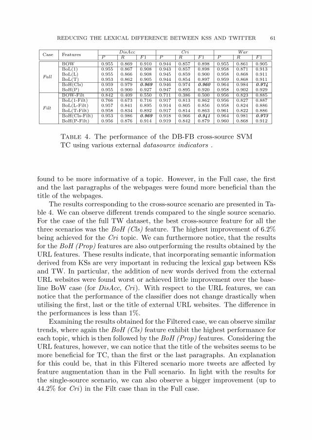
REDUCING THE LEXICAL DIFFERENCE BETWEEN KSS AND TWITTER 61
Case FeaturesDisAcc Cri War
P R F1 P R F1 P R F1
Full
BOW 0.955 0.869 0.910 0.944 0.857 0.898 0.955 0.861 0.905BoL(1) 0.955 0.867 0.908 0.943 0.857 0.898 0.958 0.871 0.913BoL(L) 0.955 0.866 0.908 0.945 0.859 0.900 0.958 0.868 0.911BoL(T) 0.953 0.862 0.905 0.944 0.854 0.897 0.959 0.868 0.911BoH(Cls) 0.959 0.979 0.969 0.946 0.974 0.960 0.964 0.984 0.974BoH(P) 0.955 0.900 0.927 0.947 0.895 0.920 0.958 0.902 0.929
Filt
BOW-Filt 0.842 0.409 0.550 0.711 0.386 0.500 0.956 0.823 0.885BoL(1-Filt) 0.766 0.673 0.716 0.917 0.813 0.862 0.956 0.827 0.887BoL(L-Filt) 0.957 0.841 0.895 0.914 0.805 0.856 0.958 0.824 0.886BoL(T-Filt) 0.958 0.834 0.892 0.917 0.814 0.863 0.961 0.822 0.886BoH(Cls-Filt) 0.953 0.986 0.969 0.918 0.966 0.941 0.964 0.981 0.973BoH(P-Filt) 0.956 0.876 0.914 0.919 0.842 0.879 0.960 0.868 0.912
Table 4. The performance of the DB-FB cross-source SVMTC using various external datasource indicators .
found to be more informative of a topic. However, in the Full case, the firstand the last paragraphs of the webpages were found more beneficial than thetitle of the webpages.
The results corresponding to the cross-source scenario are presented in Ta-ble 4. We can observe different trends compared to the single source scenario.For the case of the full TW dataset, the best cross-source feature for all thethree scenarios was the BoH (Cls) feature. The highest improvement of 6.2%being achieved for the Cri topic. We can furthermore notice, that the resultsfor the BoH (Prop) features are also outperforming the results obtained by theURL features. These results indicate, that incorporating semantic informationderived from KSs are very important in reducing the lexical gap between KSsand TW. In particular, the addition of new words derived from the externalURL websites were found worst or achieved little improvement over the base-line BoW case (for DisAcc, Cri). With respect to the URL features, we cannotice that the performance of the classifier does not change drastically whenutilising the first, last or the title of external URL websites. The difference inthe performances is less than 1%.
Examining the results obtained for the Filtered case, we can observe similartrends, where again the BoH (Cls) feature exhibit the highest performance foreach topic, which is then followed by the BoH (Prop) features. Considering theURL features, however, we can notice that the title of the websites seems to bemore beneficial for TC, than the first or the last paragraphs. An explanationfor this could be, that in this Filtered scenario more tweets are affected byfeature augmentation than in the Full scenario. In light with the results forthe single-source scenario, we can also observe a bigger improvement (up to44.2% for Cri) in the Filt case than in the Full case.

62 ANDREA VARGA, AMPARO CANO, FABIO CIRAVEGNA, AND YULAN HE
5. Challenges and Limitations
In this work we enriched the representation of short text messages withinformation from external websites with the goal of reducing the lexical dif-ferences between KSs and Twitter.
One of such external link indicators were the hashtags from a Tweet,for which we assigned a DBpedia and Freebase URI using a simple wordmatching approach. We encountered various challenges, given that hash-tags can often contain: (1) abbreviations (e.g. #nkorea http://dbpedia.
org/resource/North_Korea); (2) contain compound words (e.g. #flightdelayhttp://dbpedia.org/resource/Flight_delay); and (3) some of the hastagsmay contain new abbreviations not present in KSs (e.g. #emfrmf) . For thosecases no semantic meaning was assigned to them. In addition, one hashtag asany other word (#beirut) may have multiple meanings (e.g. the capital city ofLebanon; or a Lebanese governorate), and thus in order to assign the correctDB and FB URI one may apply a word sense disambiguation algorithm ([15])first, which takes into account not only the lexical form of a hashtag but alsothe context of the hashtag.
The automatic extraction of sentences and paragraphs from external web-sites also poses challenges. One of the main problems considering this taskis the accurate identification of boundaries on a page, since different websitesemploy different formats for describing the content of their pages. Particularlyin pages where users can add comments (e.g. newswire articles and forum-likepages) the identification of the last paragraphs becomes challenging. In ourwork we parsed a full webpage as a whole, independently of whether the lastpart of the page referred to users’ comments or not.
6. Conclusion and Future work
This study presented an approach for incorporating various backgroundinformation into cross-source TCs built on multiple linked KSs. The goalof our study was to investigate whether incorporating such information canfurthermore reduce the lexical differences between KSs and Twitter -imposedby the short length nature of Tweet messages-, thus allowing the creation ofmore accurate TC of Tweets.
We looked at two Twitter specific indicators including hashtags and URLs,for which we derived additional lexical and semantic features for training cross-source TCs. Our results on both sole Twitter and cross-source settings revealthat the indicator which provides a better feature enrichment, and thereforebetter classification performance was the hashtags.
Our future effort will consist on investigating alternative ways for bridgingthe gap between KSs and Twitter. One possible future direction could be to

REDUCING THE LEXICAL DIFFERENCE BETWEEN KSS AND TWITTER 63
investigate the impact of tweet normalisation approaches for cross-source TC,aiming at resolving the abbreviation, misspelling to standard English words([4])3
7. References
[1] Amparo Elizabeth Cano, Andrea Varga, Matthew Rowe, Fabio Ciravegna, and YulanHe. Harnessing linked knowledge sources for topic classification in social media. In 24thACM Conference on Hypertext and Social Media, HT ’13. ACM, 2013.
[2] A. Garcia-Silva, Oscar Corcho, and J. Gracia. Associating semantics to multilingualtags in folksonomies, 2010.
[3] Yegin Genc, Yasuaki Sakamoto, and Jeffrey V. Nickerson. Discovering context: classify-ing tweets through a semantic transform based on wikipedia. In Proceedings of the 6thinternational conference on Foundations of augmented cognition: directing the future ofadaptive systems, FAC’11, pages 484–492, Berlin, Heidelberg, 2011. Springer-Verlag.
[4] Bo Han and Timothy Baldwin. Lexical normalisation of short text messages: makn sensa #twitter. In Proceedings of the 49th Annual Meeting of the Association for Computa-tional Linguistics: Human Language Technologies - Volume 1, HLT ’11, pages 368–378,Stroudsburg, PA, USA, 2011. Association for Computational Linguistics.
[5] Stephanie Husby and Denilson Barbosa. Topic classification of blog posts using distantsupervision. In Proceedings of the Workshop on Semantic Analysis in Social Media,pages 28–36, Avignon, France, April 2012. Association for Computational Linguistics.
[6] Baichuan Li, Xiance Si, Michael R. Lyu, Irwin King, and Edward Y. Chang. Questionidentification on twitter. In Proceedings of the 20th ACM international conference onInformation and knowledge management, CIKM ’11, pages 2477–2480, New York, NY,USA, 2011. ACM.
[7] Edgar Meij, Wouter Weerkamp, and Maarten de Rijke. Adding semantics to microblogposts. In Proceedings of the fifth ACM international conference on Web search and datamining, WSDM ’12.
[8] Matthew Michelson and Sofus A. Macskassy. Discovering users’ topics of interest ontwitter: a first look. In Proceedings of the fourth workshop on Analytics for noisy un-structured text data, AND ’10, New York, NY, USA, 2010.
[9] D. Milne and I. H. Witten., editors. Learning to link with Wikipedia. 2008.
[10] Oscar Munoz Garcıa, Andres Garcıa-Silva, Oscar Corcho, Manuel de laHiguera Hernandez, and Carlos Navarro. Identifying Topics in Social Media Posts usingDBpedia. In Meunier Jean-Dominique, Halid Hrasnica, and Florent Genoux, editors,Proceedings of the NEM Summit, pages 81–86. NEM Initiative, Eurescom ? the Eu-ropean Institute for Research and Strategic Studies in Telecommunications ? GmbH,September 2011.
3In this work, we performed some initial experiments applying a dictionary based ap-proach for Tweet normalisation. We built a lexicon from http://www.noslang.com/ website,consisting of 5,407 abbreviation word pairs, and replaced all abbreviations found in tweetswith standard English terms. Our initial results, however, showed no improvement upon thebaseline model without normalisation. Our future work will thus aim to investigate othertweet normalisation approaches too.

64 ANDREA VARGA, AMPARO CANO, FABIO CIRAVEGNA, AND YULAN HE
[11] Takeshi Sakaki, Makoto Okazaki, and Yutaka Matsuo. Earthquake shakes twitter users:real-time event detection by social sensors. In Proceedings of the 19th internationalconference on World wide web, WWW ’10, pages 851–860, New York, NY, USA, 2010.ACM.
[12] Beaux Sharifi, Hutton, Mark-Anthony, and Jugal Kalita. Summarizing microblogs auto-matically. In Human Language Technologies: The 2010 Annual Conference of the NorthAmerican Chapter of the Association for Computational Linguistics, HLT ’10, pages685–688, Stroudsburg, PA, USA, 2010. Association for Computational Linguistics.
[13] Yangqiu Song, Haixun Wang, Zhongyuan Wang, Hongsong Li, and Weizhu Chen. Shorttext conceptualization using a probabilistic knowledgebase. In IJCAI, pages 2330–2336,2011.
[14] Ke Tao, Fabian Abel, Claudia Hauff, and Geert-Jan Houben. What makes a tweetrelevant for a topic? In Making Sense of Microposts (#MSM2012), pages 49–56, 2012.
[15] Doina Tatar. Word sense disambiguation by machine learning approach: A short survey.Fundam. Inf., July 2004.
[16] Irina Temnikova, Dogan Biyikli, and Francis Boon. First steps towards implementing asahana eden social media dashboard. In Proceedings of the conference Social Media andSemantic Technologies in Emergency Response (SMERST 2013), Coventry, UK, 2013.
[17] Andrea Varga, Amparo Elizabeth Cano, and Fabio Ciravegna. Exploring the similaritybetween social knowledge sources and twitter for cross-domain topic classification. InProceedings of the Knowledge Extraction and Consolidation from Social Media, 11thInternational Semantic Web Conference (ISWC2012), 2012.
[18] Daniele Vitale, Paolo Ferragina, and Ugo Scaiella. Classification of short texts by de-ploying topical annotations. In ECIR, pages 376–387, 2012.
[19] Tan Xu and Douglas W. Oard. Wikipedia-based topic clustering for microblogs. Proc.Am. Soc. Info. Sci. Tech., 48(1):1–10, 2011.
(1) The Organisations, Information and Knowledge (OAK) Group, Depart-ment of Computer Science, University of Sheffield, UK
E-mail address: [email protected]
(2) School of Engineering and Applied Science, Aston University, UKE-mail address: [email protected]
E-mail address: [email protected]
E-mail address: [email protected]

STUDIA UNIV. BABES–BOLYAI, INFORMATICA, Volume LVIII, Number 2, 2013
WEIGHTED MAJORITY RULE FOR HYBRID CELLULAR
AUTOMATA TOPOLOGY AND NEIGHBORHOOD
ANCA ANDREICA(1) AND CAMELIA CHIRA(1)
Abstract. Evolution rules for Cellular Automata (CAs) able to performcomputational tasks which require global coordination highlight an inter-esting emergent behavior. CAs can generate this complex behavior startingfrom a simple initial configuration based on the local interaction of simplecomponents that evolve according to some state change rule. However, thedetection of rules that exhibit coordinated global information processing isa very challenging task highly important in the study of complex systems.In this paper, we propose a new weighted rule for a cellular automaton withhybrid topology and neighborhood in which the state of a cell changes ac-cording to the cell itself and both local and long-distance cells. In theproposed approach, each cell in the neighborhood has a different weight(determined using an evolutionary algorithm) in the decision of changingthe state for the current cell. Computational experiments focus on thewell-known density classification task for the one-dimensional binary-stateCA. Results support a better performance of the proposed weighted rulecompared to the standard majority rule applied to the same CA topology.
1. Introduction
Cellular Automata (CAs) represent useful and important tools in the studyof complex systems and interactions. A cellular automaton is a system evolv-ing in discrete time steps with a discrete spatial geometry (usually a regularlattice). The CA is specified in terms of rules that define how it changes andevolves in time. A global coordinated behavior results from the local interac-tion of simple components [25, 15]. The emergent behavior and computational
Received by the editors: March 30, 2013.2010 Mathematics Subject Classification. 68-02.1998 CR Categories and Descriptors. I.2.8 Computing Methodologies [Artificial Intel-
ligence]: Problem Solving, Control Methods, and Search – Heuristic methods.Key words and phrases. evolutionary algorithms, density classification task, cellular
automata.This paper has been presented at the International Conference KEPT2013: Knowledge
Engineering Principles and Techniques, organized by Babes-Bolyai University, Cluj-Napoca,July 5-7 2013.
65

66 ANCA ANDREICA AND CAMELIA CHIRA
complexity of a system can be analyzed and better understood based on CAdynamics [2].
One of the most widely studied CA problems is the density classificationtask (DCT) [10, 21, 16, 18, 2]. This is a prototypical distributed computationaltask with the objective of finding the density most present in the initial cellularstate. The discovery of rules exhibiting a high degree of global self-organizationis not easily achieved. DCT is not a trivial task since coordinated globalinformation processing must rise from the interactions of components withlocal information and communication.
Most existing studies [6, 3, 15, 9, 16, 20, 14, 11, 18] focus on developingalgorithms able to find high performant rules for one-dimensional CAs withfixed neighborhood size. Each iteration, the change of a cell state dependson the cell itself and r local cells neighbors on each side. In this case, theneighborhood size is fixed to 2 ∗ r + 1 and the method searches for the bestrule able to correctly classify potentially any initial configuration. Network-based CAs have also been investigated in the context of DCT [23, 24, 4, 5, 22].The topology of the CA is given by a general graph and the neighborhood ofeach cell varies with the number of connecting nodes in the graph while the ruleremains fixed (i.e. the majority rule). For network-based CAs, algorithms aredesigned to search for the graph topology that triggers the best neighborhoodto be used in connection with a fixed rule for the DCT. Another topologyproposed in [1] is a hybrid one in which the state change of a cell is allowed tobe influenced by long-distance cells. Besides the cell itself and the cells in thelocal neighborhood, fixed distant cells contribute to the way in which the cellstate is changed over time. This hybrid neighborhood has a fixed structurecombining local and, to a certain extent, global information.
In this paper, we propose a new weighted rule that can be applied for thehybrid topology mentioned above. In the proposed approach, the local neigh-bors and the long-distance neighbors have different weights when computingthe next state of a current cell. An evolutionary algorithm is developed tosearch for the best performing weighted rule for DCT based on the hybridneighborhood structure. Computational experiments indicate a better per-formance obtained by the proposed weighted rule compared to the standardmajority rule for hybrid CA topology and neighborhood.
The rest of the paper is structured as follows: section 2 briefly presents thedensity classification problem, section 3 describes the relevant lattice, network-based and hybrid CA topologies, section 4 presents the proposed weightedmajority rule, section 5 includes the computational experiments and results,and section 6 contains the conclusions of the paper and directions for futurework.

WEIGHTED MAJORITY RULE FOR HYBRID CELLULAR AUTOMATA 67
2. The Density Classification Problem
DCT is a challenging problem extensively studied due to its simple de-scription and potential to generate a variety of complex behaviors.
The aim of DCT is to find a binary one-dimensional CA able to classifythe density of 1s (denoted by ρ0) in the initial configuration. If ρ0 > 0.5 (1 isdominant in the initial configuration) then the CA must reach a fixed pointconfiguration of 1s otherwise it must reach a fixed-point configuration of 0swithin a certain number of timesteps. Most studies consider the CA length ofN = 149 and the CA radius of r = 3 (which gives a neighborhood size of 7).
The CA lattice starts with a given binary string called the initial configu-ration (IC). After a maximum number of iterations (usually set as twice thesize of CA), the CA will reach a certain configuration. If this is formed ofhomogeneous states of all 1s or 0s, it means that the IC has been classified asdensity class 1, respectively 0. Otherwise, the CA makes by definition a mis-classification [20]. It has been shown that there is no rule that can correctlyclassify all possible ICs [13].
The performance of a rule measures the classification accuracy of a CAbased on the fraction of correct classifications over ICs selected from an unbi-ased distribution (ρ0 is centered around 0.5).
3. CA Topologies and Results for DCT
This section describes some relevant CA topologies, i.e. lattice, networkand hybrid, and presents related existing rule detection methods and theirresults for DCT.
3.1. Regular Lattice Topology. A one-dimensional lattice of N two-statecells is used to represent the CA. The state of each cell changes according toa function depending on the current states in the neighborhood. The neigh-borhood of a cell is given by the cell itself and its r neighbors on both sidesof the cell, where r represents the radius of the CA. The initial configurationof cell states (0s and 1s) for the lattice evolves in discrete time steps updatingcells simultaneously according to the CA rule.
The regular lattice topology is engaged in most studies tackling DCTfor 1D binary-state CA. Packard [19] developed the first evolutionary ap-proach to detect rules for one dimensional binary state CA with a radiusof 3. The potential of genetic algorithms for computational emergence in thedensity classification task has been extensively investigated by Mitchell et al[6, 3, 15, 9, 16, 20, 14]. The evolutionary approach to DCT proposed byMitchell et al sets the fitness of a rule table as the fraction of correct classifi-cations made over 100 randomly chosen initial configurations with uniformly

68 ANCA ANDREICA AND CAMELIA CHIRA
distributed density. The three main strategies discovered are default, block-expanding (a refinement of the default strategy) and particle revealing increas-ing computational complexity [3]. The best particle rule found by Mitchell etal [15] has a performance of 0.769.
Juille and Polack [11] used coevolutionary learning for the density clas-sification task reporting good results for this problem (performance of 0.86).Oliveira et al [17] present a multiobjective evolutionary approach to DCTbased on the non-dominated sorting genetic algorithm (NSGA). The algo-rithm is implemented in a distributed cooperative computational environmentand is able to discover new rules with a performance of 0.8616. Wolz andOliveira [26] proposed a two-tier evolutionary framework able to detect ruleswith a performance of 0.889. The approach integrates a basic evolutionaryalgorithm in a parallel multi-population search algorithm. To the best of ourknowledge, the DCT rules presented in [26] are the ones with best performancediscovered to date [18].
3.2. Network Topology. Some studies [23, 24, 4, 5, 22] consider a network-based topology for the CA where the cells can be connected in any way whilethe rule is the same for all cells.
Watts [24] studied the small-world graph version of the DCT: the ruleis fixed and the performance of different small-world networks for DCT isevaluated. A small-world graph is constructed starting from a regular ringof nodes in which each node has k neighbors followed by a random rewiringprocedure [23, 24]. The rule used for small-world network DCT is simple:at each time step, each node takes the state of the majority of its neighbornodes in the graph (if the number of state 1s equals the number of state 0sin the neighbors list then the node is randomly assigned a state with equalprobability between 0 and 1). Small-world networks have a performance ofaround 0.8 for the DCT with this fixed majority rule for 149 cells CA.
Tomassini et al [4, 5, 22] investigated network-based CAs for the densityand synchronization problems. Spatially structured evolutionary algorithmsare used to find the best performant network topology for DCT when the ruleis fixed to the majority rule. An individual represents a network structure andthe fitness is computed based on the fraction of ICs (out of 100 ICs generatedanew for each individual) correctly classified by the majority rule based onthe neighborhood given by the network. The best evolved network startingfrom initial regular rings has a performance of 0.823 (for 149 cells) whilethe result for random graphs as initial population is similar (performance of0.821 of the best network). Similar results have been obtained by [8] with asimple evolutionary algorithm able to produce network topologies with highperformance for DCT based on the majority rule.

WEIGHTED MAJORITY RULE FOR HYBRID CELLULAR AUTOMATA 69
3.3. Hybrid Topology. A hybrid topology has been proposed in [1] where amixed induced neighborhood keeps invariable the number of neighbors. Thistopology works on a lattice based on the CA radius r and a parameter nreferring to the number of long-distance cells allowed to contribute to thecurrent hybrid neighborhood. In order to create the new topology of radius r,we start with a regular ring lattice of radius r−n. The other 2 ∗n nodes thatare part of the hybrid neighborhood of a node i are long distance neighborsrandomly chosen from the rest of the nodes, but following some rules thatensure the equilibrium of the neighborhood. This means that i always remainsthe central node of the neighborhood and the distance between node i and thelong distance neighbors places half of them (n nodes) on the left hand sideand the other half (n nodes) on the right hand side of i. Using this approach,a new topology which resembles a network topology but it is still very closeto a regular ring lattice is obtained. This allows us to consider the samemajority understanding as in the classical case of regular ring lattice topology.A detailed description of the proposed hybrid topology can be found in [1].
The potential of this topology with the corresponding notion of hybridneighborhood is shown by the significantly better performance obtained infewer CA iterations, compared to the classical approach that uses the regu-lar ring lattice as topology. We should also note that the best performanceobtained with the hybrid topology (0.79) is considerably higher than the per-formance obtained for regular lattice topology (0.64) and is very close to theperformance obtained by CA based on small-world topologies (0.82).
4. New Weighted Rule for Cellular Automata with HybridNeighborhood
As already mentioned, the state of each cell in CA changes according to afunction depending on the current states in the neighborhood. The neighbor-hood of a cell is given by the cell itself and its r neighbors on both sides of thecell. The initial configuration of cell states (0s and 1s) for the lattice evolvesin discrete time steps updating cells simultaneously according to the CA rule.
In current existing approaches, each neighbor (including the cell itself) hasthe same vote weight when deciding which is the next state of the current cell.Indeed, whether we consider the regular lattice ring or the network topologyfor CAs, we can not differentiate between neighbors - the vote of each neighborhas the same weight. The hybrid topology described in the previous sectionallows us to introduce a new concept of majority rule, where different neighborshave different vote weights when deciding the next state of the current cell.
The hybrid topology involves the presence of two kinds of neighbors: localand far neighbors. The proposed rule gives different vote weights to local

70 ANCA ANDREICA AND CAMELIA CHIRA
neighbors and to far neighbors. Let us denote by wl the weight assigned tolocal neighbors and by wf the weight assigned to far neighbors. We identifytwo different scenarios that can be applied in this approach:
(i)0 ≤ wl ≤ 1, wf = 1− wl
(ii)0 ≤ wl ≤ 1, 0 ≤ wf ≤ 1
In the first scenario, the increase of one weight leads to the decrease ofthe other one, while in the second scenario, there is no relation between theweights of the two kinds of neighbors. In both scenarios, we compute themaximum weighted sum that can be obtained when each neighbor has thevalue 1. Let us denote by wmax the obtained value:
wmax = nl ∗ wl + nf ∗ wf ,
where nl represents the number of local neighbors and nf represents the num-ber of far neighbors.
Let sti denote the state of cell i at timestep t. Let ij , where j = 1, 2r + 1,represent the neighbors of cell i. The number of neighbors of a cell is 2∗ r+1,out of which nl = 2∗(r−n) are local neighbors and nf = 2∗n are far neighbors,according to the hybrid topology.
For each cell i, the weighted sum of the neighbors states at timestep t,denoted by σt
i , is defined as follows:
σti =
2r+1∑j=1
stij ∗ wij
As indicated above, stij represents the state of cell ij in the hybrid neigh-
borhood at timestep t and wij is the weight of neighbor ij :
wij =
{wl, if ij is a local neighbor
wf , if ij is a far neighbor
The next state of a cell i is 1 if the weighted sum σi exceeds half of themaximum weighted sum:

WEIGHTED MAJORITY RULE FOR HYBRID CELLULAR AUTOMATA 71
st+1i =
{1, if σt
i ≥ wmax/2
0, otherwise
The proposed weighted rule is a very realistic model with many appli-cations in real-world problems where different entities have different votingweights when deciding a next state in a system that could be modeled as aCA.
5. Experimental Results
Computational experiments consider a well studied version of the DCTproblem: the one-dimensional binary-state CA of size 149 based on the radiusof 3. For the hybrid topology we set r = 3 and n = 1 (i.e. 2 local neighborson each side and 1 distant neighbor). The neighborhood size is 7 cells whichleads to a rule size of 27 = 128.
A simple evolutionary algorithm has been developed to detect rules for theDCT. A potential solution of the problem is encoded as a one-dimensional ar-ray of weights (one weight for the first proposed scenario and two weightsfor the second one). The initial population is randomly generated. Thepotential solutions are evaluated by means of a real-valued fitness functionf : X → [0, 1], where X denotes the search space of the problem. The fitnessfunction represents the fraction of correct classification over 100 randomlygenerated initial configurations. A relative fitness is used, as the set of initialconfigurations is generated anew for each generation of the algorithm. Thisway, solutions with high fitness in one generation and which survive in thenext generation will be evaluated again using another set of 100 initial con-figurations. While the fitness is evaluated by using 100 uniformly distributedinitial configurations, the performance of a rule is computed as the fraction ofcorrect classifications for 104 randomly generated initial configurations. Theinitial configurations are generated in such a way that each cell has the sameprobability 1
2 of being 0 or 1. The CA is iterated until it reaches a fixed-pointconfiguration of 1s or 0s but for no more than M ≈ 2N time steps.
The individual resulted after each recombination will be mutated at ex-actly two randomly chosen positions. A weak mutation is considered, theprobability of obtaining a different value for the chosen position being equalto the probability of obtaining the very same value. The algorithm is appliedfor 100 generations with a population size of 100, roulette selection, one pointcrossover with probability of 0.8, weak mutation with probability 0.2 and elitesize of 10%.

72 ANCA ANDREICA AND CAMELIA CHIRA
Table 1. Performance obtained in 10 runs for HybCA,W1HybCA and W2HybCA
HybCA W1HybCA W2HybCA
Best 0.7902 0.8202 0.8083
Average 0.74847 0.79475 0.76573
Std Dev 0.034297815 0.017707202 0.0374052
T-test p-value 0.001870 0.364680
The performance obtained with the new weighted majority rule (both sce-narios) is compared to the performance obtained when using the classical ruletable. It should be noted that the same evolutionary algorithm with the sameparameters is used to evolve both standard and weighted rules in order toallow a direct comparison of results. Both standard and weighted rules usethe same hybrid CA topology and neighborhood. The case of standard rulescan be viewed as a simplification of weighted rules evolution where no weightsneed to be determined.
Table 1 presents the results obtained after 10 runs of the algorithm todetect a classical rule (HybCA) and for evolving a weighted rule (W1HybCAfor first scenario and W2HybCA for the second scenario considered). Theweighted rule triggers an improvement of performance from 0.7902 (HybCA)to 0.8202 for W1HybCA and 0.8083 for W2HybCA. The results are comparedusing the paired t-test with a 95% confidence interval. For the first scenario,the p-value is significantly smaller than 0.05, which indicates that the meanperformance obtained when using the proposed weighted rule is notably bet-ter than that obtained when using a classical rule. The mean performanceobtained based on the second scenario is higher compared to the classical rulebut not significantly (according also to the p-value which is higher than 0.05 asshown in Table 1). The best performance obtained in 10 runs of the evolution-ary algorithm is indeed more significantly improved when using the weightedrule in the first scenario (the evolved weight for local neighbors was 0.16 whenthe best performance was obtained). Therefore, we further consider this firstscenario to perform a further analysis and report results.
A comparison that shows the efficiency of the proposed weighted rule is thenumber of iterations needed to correctly classify the initial configurations (forexample, for a performance of 0.82, there are 8200 correctly classified initial
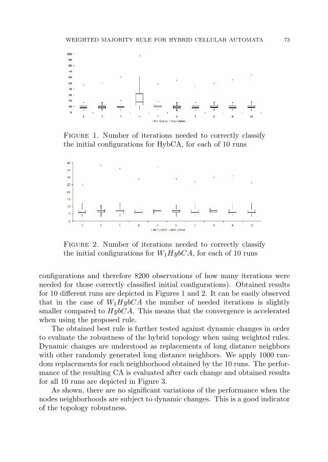
WEIGHTED MAJORITY RULE FOR HYBRID CELLULAR AUTOMATA 73
Figure 1. Number of iterations needed to correctly classifythe initial configurations for HybCA, for each of 10 runs
Figure 2. Number of iterations needed to correctly classifythe initial configurations for W1HybCA, for each of 10 runs
configurations and therefore 8200 observations of how many iterations wereneeded for those correctly classified initial configurations). Obtained resultsfor 10 different runs are depicted in Figures 1 and 2. It can be easily observedthat in the case of W1HybCA the number of needed iterations is slightlysmaller compared to HybCA. This means that the convergence is acceleratedwhen using the proposed rule.
The obtained best rule is further tested against dynamic changes in orderto evaluate the robustness of the hybrid topology when using weighted rules.Dynamic changes are understood as replacements of long distance neighborswith other randomly generated long distance neighbors. We apply 1000 ran-dom replacements for each neighborhood obtained by the 10 runs. The perfor-mance of the resulting CA is evaluated after each change and obtained resultsfor all 10 runs are depicted in Figure 3.
As shown, there are no significant variations of the performance when thenodes neighborhoods are subject to dynamic changes. This is a good indicatorof the topology robustness.

74 ANCA ANDREICA AND CAMELIA CHIRA
Figure 3. Performance obtained in 1000 dynamic steps for 10runs of the algorithm
Figure 4. Performance obtained in 1000 dynamic steps forone run of the algorithm
Figure 4 presents the results obtained by a typical run of the algorithm(from the considered 10 runs). The original performance of the obtained rulebefore the topology being subject to dynamic changes was 0.8202. It can benoticed that the performance does not go below 0.7545, we even obtain betterperformances (the best one is 0.8362) and an average performance of 0.7977.
6. Conclusions and Future Work
A new weighted rule for a hybrid CA topology and neighborhood has beenproposed. The cells in the hybrid neighborhood are allowed to have differ-ent weights (according to their local or far association to the current cell)in the decision of changing the current cell state. This approach enables aweighted rule application to the hybrid CA topology which has been inves-tigated for the DCT in one-dimensional binary state CAs. Computationalexperiments emphasize that the weighted rules detected by an evolutionaryalgorithm have a good performance shown to improve that of standard rules

WEIGHTED MAJORITY RULE FOR HYBRID CELLULAR AUTOMATA 75
evolved for the same CA topology. The CA performance remains stable whendynamic changes are introduced in the neighborhood structure.
Future work focuses on investigating weighted schemes in connection withother CA rules and topologies, particularly for network-based CAs whereweights associated with edges connecting two cells can be easily used in aweighted majority rule for graph topologies.
Acknowledgment
This research is supported by Grant PN II TE 320, Emergence, auto-organization and evolution: New computational models in the study of com-plex systems, funded by CNCSIS, Romania.
References
[1] Andreica, A., Chira, C., Using a Hybrid Cellular Automata Topology and Neighborhoodin Rule Discovery, submitted to IEEE Congress on Evolutionary Computation (CEC2013).
[2] Chira, C., Gog, A., Lung, R. I., Iclanzan, D., Complex Systems and Cellular AutomataModels in the Study of Complexity, Studia Informatica series, Vol. LV, No. 4, pp. 33-49(2010)
[3] Crutchfield, J.P., Mitchell, M., The evolution of emergent computation, Proceedings ofthe National Academy of Sciences, USA 92 (23), (1995), pp.10742-10746.
[4] Darabos, C., Giacobini, M., Tomassini, M., Performance and Robustness of CellularAutomata Computation on Irregular Networks. Advances in Complex Systems 10: 85-110 (2007)
[5] Darabos, C., Tomassini, M., Di Cunto, F., Provero, P., Moore, J.H., Giacobini, M.,Toward robust network based complex systems: from evolutionary cellular automata tobiological models, Intelligenza Artificiale 5(1): 37-47 (2011)
[6] Das, R., Mitchell, M., Crutchfield, J.P., A genetic algorithm discovers particle-basedcomputation in cellular automata, Parallel Problem Solving from Nature Conference(PPSN-III), Springer-Verlag (1994) pp.344-353.
[7] Ferreira, C., Gene Expression Programming: A New Adaptive Algorithm for SolvingProblems, Complex Systems, Vol. 13, No. 2 (2001), pp.87-129.
[8] Gog, A., Chira, C., Dynamics of Networks Evolved for Cellular Automata Computation,Proceedings of the 7th International Workshop on Hybrid Artificial Intelligence Systems(HAIS 2012), Salamanca, Spain, Hybrid Artificial Intelligent Systems, Springer-Verlag,vol. 7208-7209 (2012) pp. 359-368.
[9] Hordijk, W., Crutchfield, J.P., Mitchell, M., Mechanisms of Emergent Computation inCellular Automata, Parallel Problem Solving from Nature-V, Springer-Verlag (1998)pp.613-622.
[10] Juille, H., Pollack, J.B.: Coevolving the ’ideal’ trainer: Application to the discovery ofcellular automata rules. Genetic Programming 1998: Proceedings of the Third AnnualConference (1998)
[11] Juille, H., Pollack, J.B., Coevolutionary learning and the design of complex systems,Advances in Complex Systems, Vol. 2, No. 4 (2000), pp. 371-394.

76 ANCA ANDREICA AND CAMELIA CHIRA
[12] Koza, J.R., Genetic Programming: On the Programming of Computers by Means ofNatural Selection, MIT Press, Cambridge (1992).
[13] Land, M., Belew, R. K., No perfect two-state cellular automata for density classificationexists, Physical Review Letters, 74:25 (1995), pp. 5148-5150.
[14] Marques-Pita, M., Mitchell, M., Rocha, L., The role of conceptual structure in designingcellular automata to perform collective computation, Proceedings of the Conference onUnconventional Computation, UC 2008, Springer (Lecture Notes in Computer Science),2008.
[15] Mitchell, M., Crutchfield, J.P., Das, R., Evolving cellular automata with genetic algo-rithms: A review of recent work, In Proceedings of the First International Conferenceon Evolutionary Computation and Its Applications (EvCA’96). Russian Academy ofSciences (1996)
[16] Mitchell, M., Thomure, M. D., Williams, N. L.: The role of space in the Success of Co-evolutionary Learning. Proceedings of ALIFE X - The Tenth International Conferenceon the Simulation and Synthesis of Living Systems (2006)
[17] de Oliveira, P.P.B., Bortot, J.C., Oliveira, G., The best currently known class of dy-namically equivalent cellular automata rules for density classification, Neurocomputing,70:1-3 (2006), pp. 35-43.
[18] Oliveira, G.M.B., Martins, L.G.A., de Carvalho, L.B., Fynn, E., Some investigationsabout synchronization and density classification tasks in one-dimensional and two-dimensional cellular automata rule spaces, Electron. Notes Theor. Comput. Sci., 252(2009), pp. 121-142.
[19] Packard, N.H., Adaptation toward the edge of chaos, Dynamic Patterns in ComplexSystems, World Scientific (1988), pp. 293-301.
[20] Pagie, L., Mitchell, M.: A comparison of evolutionary and coevolutionary search. Int.J. Comput. Intell. Appl., 2, 1, 53-69 (2002)
[21] Tomassini, M., Venzi, M.: Evolution of Asynchronous Cellular Automata for the DensityTask. Parallel Problem Solving from Nature - PPSN VII, Lecture Notes in ComputerScience, Springer Berlin / Heidelberg, 2439, 934-943 (2002)
[22] Tomassini, M., Giacobini, M., Darabos, C., Evolution and dynamics of small-worldcellular automata, Complex Systems 15 (2005), pp. 261-284.
[23] Watts, D.J., Strogatz, S.H., Collective dynamics of ’smallworld’ networks, Nature 393(1998), pp. 440-442.
[24] Watts, D.J., Small Worlds: The Dynamics of Networks Between Order and Randomness,Princeton University Press, Princeton, NJ (1999)
[25] Wolfram, S., Theory and Applications of Cellular Automata, Advanced series on com-plex systems, World Scientific Publishing, 9128 (1986)
[26] Wolz, D., de Oliveira, P.P.B., Very effective evolutionary techniques for searching cel-lular automata rule spaces, Journal of Cellular Automata 3 (2008), pp. 289-312.
(1) Babes-Bolyai University, Department of Computer Science, Cluj-Napoca,Romania
E-mail address: [anca,cchira]@cs.ubbcluj.ro

STUDIA UNIV. BABES–BOLYAI, INFORMATICA, Volume LVIII, Number 2, 2013
PEDESTRIAN RECOGNITION BY USING KERNEL
DESCRIPTORS
ANCA ANDREICA, LAURA DIOSAN, RADU GACEANU, AND ADELA SIRBU(1)
Abstract. Recognition of people in images is important for many appli-cations in computer vision. This paper presents an experimental studyon pedestrian classification. We investigate the recently developed kernel-based features in order to represent an image and two learning algorithms:the popular Support Vector Machine (SVM) and Genetic Programming(GP). Numerical experiments are performed on a benchmark dataset con-sisting of pedestrian and non-pedestrian (labeled) images captured in out-door urban environments and indicate that the evolutionary classifier isable to perform better over SVM.
1. Introduction
Pedestrian safety is an important problem of global dimensions. A WorldHealth Organization 2010 report describes traffic accidents as one of the majorcause of death and injuries around the world, accounting for an estimated 1.2million fatalities and 50 million injuries. Enhancing comfort and safety forthe driver and the occupants of an automobile has been a major motivatorin innovations associated with Intelligent Vehicles and Intelligent Transporta-tion Systems. The European Union has been conducting several projects incollaboration with auto industry and research institutes for intelligent vehiclesystems in general and pedestrian safety in particular.
One approach for pedestrian safety improvement is to develop performantrecognition systems. In this paper we propose an evolutionary-based modelfor the learning phase of such a system. The input data for this classifier is
Received by the editors: March 25, 2013.2010 Mathematics Subject Classification. 68T05,91E45.1998 CR Categories and Descriptors. code I.2.6 [Learning]: – Concept learning .Key words and phrases. Object recognition, Kernel descriptors, Support Vector Machines,
Kernel selection.This paper has been presented at the International Conference KEPT2013: Knowledge
Engineering Principles and Techniques, organized by Babes-Bolyai University, Cluj-Napoca,July 5-7 2013.
77

78 A. ANDREICA, L. DIOSAN, R. GACEANU, A. SIRBU
represented by features extracted from images by using different kernel de-scriptors.
Pedestrian detection has been an intensively studied problem, especiallyin the last years. There is a variety of classifiers in literature trained on differ-ent combinations of features like HOG [7], SURF [2], CSS [23], Haar walvetrepresentation [22] and tested on datasets like INRIA, Daimler or Caltech. In[23] is performed a comparison of the existing datasets and an evaluation ofseveral classifiers (AdaBoost, linear SVM, HIK SVM and latent SVM) basedon HOG and Haar walvet representation. One of the most efficient featureextraction methods is represented by kernel descriptors [4]. In addition, thesefeatures have not been used in the case of pedestrian recognition yet, to thebest of our knowledge. We, therefore, investigate their usage for this problem.
For solving the classification task, there are several approaches like Boost-ing [17] and statistical classification: Artificial Neural Networks (ANN) [24]and Support Vector Machines (SVM) [1]. It is known that the SVM performsbetter as it can avoid over-learning problem that appears in ANN training anda deficiency of a slow training speed that appears in Adaboost.
In our approach we involve a GP-based learning, as evolutionary methodsare able to identify a large spectrum of decision functions (linear or non-linear). Furthermore, there are no evolutionary models for solving the pedes-trian recognition problem, as far as we know.
The paper is organised as follows: Section 2 reviews the most efficientimage representations and Section 3 gives a brief description of two learningalgorithms (SVM and GP). The proposed framework is presented in Section4 and followed by numerical experiments (detailed in Section 5). Finally,conclusions and ideas for future work can be found in Section 6.
2. Image representation
A highly challenging problem in computer vision is how to extract relevantimage features. The features that characterise an image can be classified frommany points of view. An important criterion is the area from that the feature isextracted: if the entire image is used, then some global features are computed,while if one or more image regions (patches) are utilised, then local featuresare determined. Another important criterion is the complexity of extraction.Image features can be extracted from scratch that means the features areextracted directly from the image (and in this case we discuss about low-levelfeatures) or can be computed based on some previously extracted features (inthis case high-level features are obtained). The most popular (due to theirsuccess) low-level image descriptors are orientation and gradient histograms,

PEDESTRIAN RECOGNITION BY USING KERNEL DESCRIPTORS 79
while one of the best high-level descriptor is the kernel view of orientationhistograms [4]. More details about these features are given in the following.
2.1. Histogram of Oriented Gradient (HOG) descriptors. The firststep in human detection in images is represented by feature extraction. Forthis stage in the recognition process, Dalal et al [7] proposed the Histogramof Oriented Gradient (HOG) descriptors, which show superior performancecompaired to previously existing approaches (eg. SIFT [14], SURF [2], etc).HOG descriptors are briefly described in what follows.
Firstly, there is a normalization stage intended to reduce the influence ofillumination effects. Power low compression is used on this purpose. There isa second stage for computing first order image gradients for detecting contour,silhouette and some texture information. The image is then divided into smallregions called cells, for each of them accumulating a local 1-D histogram ofgradient or edge orientations over all the pixels. The combined histograms givethe image representation. A contrast-normalization follows in order to inducea better invariance to illumination, shadowing and edge contrast. Local groupsof cells form blocks that might overlap and the normalised block descriptorsare referred to as HOG descriptors. The descriptors from all blocks are thencollected into a combined feature vector.
Static version of HOG descriptors are obtained by following the stagesdescribed above. The authors also proposed motion HOG descriptors whichuse oriented histograms of differential optical flow. The gradient computationis therefore replaced by flow computation and differential flow estimation [8].
2.2. Kernel Descriptors (KD). Kernel descriptors [4] can be seen as ageneralization of orientation histograms (including HOG), which are a par-ticular type of match kernels over patches (viewed as a collection of blocks).Moreover, kernel descriptors overcome some disadvantages of histograms basedtechniques, where similarity between different regions of images is computedbased on their histogram. By using this approach, some quantization errorsmight be introduced, as individual pixel attribute values are discretized intobins and then a histogram is computed over the discrete attribute values withina patch.
Some of the kernel descriptors are the gradient match kernel (able to cap-ture image variations) – based on a kernel of magnitudes, an orientation kerneland a position kernel –, the colour kernel (able to describe image appearance)– based on a colour kernel and a position kernel – and the local binary pat-tern kernel (able to capture local shape more effectively) – based on a kernelof standard deviations of neighbour pixels, a kernel of binarized pixel valuedifferences in a local window and a position kernel.

80 A. ANDREICA, L. DIOSAN, R. GACEANU, A. SIRBU
The advantage of kernel descriptors is that they do not discretize pixelattribute values, being able to convert pixel attributes into rich patch-levelfeatures. The similarity between different images regions is therefore com-puted based on a match kernel function. For computation efficiency reasons,approximate, low dimensional match kernels are computed.
Kernel descriptors can be applied not only over sets of pixels, but oversets of kernel descriptors as well. In this hierarchical approach [3], kerneldescriptors are recursively applied until the image features are obtained.
3. Learning algorithm
Another aspect that must be considered when the problem of object recog-nition has to be solved is the classification algorithm. Since the classificationmust be performed in an automatically manner, a machine learning algorithmcan be utilised. The general problem of machine learning is to search a, usu-ally very large, space of potential hypotheses to determine the one that willbest fit the data and any prior knowledge. In supervised image classification,we are given a training set of images and their corresponding labels. The goalis to learn (based on the training set) a classifier to label unseen images. Twoof the most performant algorithms are SVM and GP-based classifiers and, inwhat follows, we will briefly describe them.
3.1. SVM. SVMs are a group of supervised learning methods that can beapplied to classification or regression. They use a technique known as the“kernel trick” to apply linear classification techniques to non-linear classifica-tion problems. Using a Kernel function [20], the data points from the inputspace are mapped into a higher dimensional space. Constructing (via the Ker-nel function) a separating hyperplane with maximum margin in the higherdimensional space yields a non-linear decision boundary in the input spaceseparating the tuples of one class from another.
Suppose the training data has the following form: D = (xi, yi)i=1,m, where
xi ∈ <d represents an input vector and each yi, yi ∈ {−1,+1}, the output labelassociated to the item xi. SVM algorithm maps the input vectors to a higherdimensional space where a maximal separating hyper-plane is constructed [20].In order to construct a maximal margin classifier one has to solve the followingconvex quadratic programming problem, which is the primal formulation ofit:
(1)minimisew,b,ξ
12w
Tw + C∑m
i=1 ξisubject to: yi(w
Tφ(xi) + b) ≥ 1− ξi,ξi ≥ 0,∀i ∈ {1, 2, . . . ,m}.

PEDESTRIAN RECOGNITION BY USING KERNEL DESCRIPTORS 81
The coefficient C (usually called penalty error or regularization parameter) isa tuning parameter that controls the trade off between maximizing the marginand classifying without error. Larger values of C might lead to linear functionswith smaller margin, allowing to classify more examples correctly with strongconfidence. A proper choice of this parameter is crucial for SVM to achievegood classification performance.
The original optimal hyper-plane algorithm proposed by Vapnik in 1963was a linear classifier [20]. However, in 1992, Boser, Guyon and Vapnik [5] havesuggested a way to create non-linear classifiers by applying the kernel trick.Kernel methods work by mapping the data items into a high-dimensionalvector space F , called feature space, where the separating hyper-plane has tobe found [5]. This mapping is implicitly defined by specifying an inner productfor the feature space via a positive semi-definite kernel function: K(x, z) =φ(x)Tφ(z), where φ(x) and φ(z) are the transformed data items x and z [19].Note that all we required is the result of such an inner product. Thereforewe neither need to have an explicit representation of the mapping φ, nor dowe need to know the nature of the feature space. The only requirement is tobe able to evaluate the kernel function on all the pairs of data items, whichis much easier than computing the coordinates of those items in the featurespace.
There is a wide choice for a positive definite and symmetric kernel K. Theselection of a kernel has to be guided by the problem that must be solved.Choosing a suitable kernel function for SVMs is a very important step for thelearning process.
While SVM classifiers intrinsically account for a trade off between modelcomplexity and classification accuracy [21], the generalization performance isstill highly dependent on appropriate selection of the penalty error C andkernel parameters.
3.2. GP. Genetic programming (GP) is a form of evolutionary computationin which the individuals in the population are computer programs, instead ofbit strings [12]. GP starts from a high-level statement of what needs to bedone and creates a computer program to solve the problem [12]. While ge-netic algorithms (GA) want to evolve only solutions for particular problems,GP evolves complex computer programs. GP individuals are represented andmanipulated as nonlinear entities, usually trees in the standard approach. Anyexpression can be represented as a tree of functions and terminals. Dependingon the problem to solve, a GP chromosome can be the syntax of an arith-metic expression, formulas in first order predicate logic or code written in aprogramming language [11].

82 A. ANDREICA, L. DIOSAN, R. GACEANU, A. SIRBU
The skeleton of a GP algorithm is similar to GA. It uses a population ofindividuals on which the standard evolutionary operators are applied. Initiallya population of hierarchically arranged programs is generated by randomlycombining functions and terminals. A fitness function may be applied on theseprograms and the best individuals are selected for reproduction. Crossover isachieved by swapping subtrees among the parents starting at two randomlyselected nodes. Mutation may occur by replacing the subtree starting at arandomly selected node in the chromosome by a randomly generated subtree[12].
Flexibility is one of the main advantages of GP, and this feature allows GPto be applied for classification in many different ways. The nature of GP in-dividuals, which include terminals (variables and constants) and nonterminals(operators and functions), gives them the ability not only to represent knowl-edge but also to perform computations, so that GP can be used in almost anyclassification-related task, not only in the core task of classifier induction, butalso for preprocessing and post-processing purposes [10]. GP can be easilyapplied to decision tree evolution considering that chromosomes are usuallyrepresented as trees and thus they could each be regarded as decision tree clas-sifiers. Along the same line, GP individuals can encode classification rules. Aclassification rule consists of two parts: the antecedent and the consequent.The antecedent states a condition over the data while the consequent con-tains the class label. The conditional part is usually composed of relationaloperators applied on various attribute data, i.e., an expression which can berepresented as a tree of functions and terminals.
4. Proposed framework
Our aim is to investigate how two different learning algorithms can solvean important classification problem: the pedestrian recognition. Since the per-formance of a classification algorithm is strongly influenced by two ingredients(first, a suitable representation of the objects to be categorized and second,a powerful decision maker algorithm on top of this representation), we havedecided to extract relevant features from images through kernel descriptorsthat must be analysed and processed by two classification methods: SVM andGP.
4.1. Arguments. Why Kernels? Because, by definition, they catch the sim-ilarity between arbitrary inputs, being able, in the same time, to integrateinvariance (that is present in the case of image processing), to capture depen-dencies and to perform an efficient computation and storage.
Why SVM? It is well known that linear SVMs are currently the mostfrequently used classifiers in Computer Vision [13] since its training time is

PEDESTRIAN RECOGNITION BY USING KERNEL DESCRIPTORS 83
approximately linear in data dimensionality and, also, approximately linearin number of training examples. Furthermore, the evaluation time (per testexample) is linear in data dimensionality and is independent of number oftraining examples. According to [13] SVMs with non-linear kernel are com-monly used for small to medium sized Computer Vision problems becausetheir training time is typically cubic in number of training examples, whiletheir evaluation time is typically linear in number of training examples. Fur-thermore, the classification accuracy is typically higher compared to linearSVMs. Shortly, linear SVMs are very fast in training and evaluation, whilenon-linear kernel SVMs give better results, but do not scale well (with respectto number of training examples).
Why GP? There are several arguments that sustain the utility of GP-basedmethods in solving classification problems, in general, and object recognition,in particular. Firstly, a GP-based method is able to perform an implicit andautomatic transformation of data (the original features can be pre-processedby different methods: selection of a subset of original attributes, weightingthe original attributes, construction of new features as functional expressionsinvolving the original attributes). The feature selection is part of the evo-lutionary process of GP that involves individuals encoded as variable-lengthchromosomes, while the feature construction benefits of the GP individual’sability to combine the attributes trough different operations. Secondly, GP isable to extract various models (like classification rules or discriminant func-tions) from data. Furthermore, due to its capability to evolve complex dis-criminant functions, GP is able to solve both linear classification problems andnon-linear classification problems without apriori specifying the problem type(linear or non-linear). When a linear classifier can not solve the problem, twosolutions can be considered:
• a combination of several linear classifiers (as in the case of ANN orBoosting which actually encode decision functions which depend non-linearly on input data) or• a data pre-processing step, when the original input data is transformed
form the original space of representation (non-linear) into a new spacethat is, in general, a higher dimensional one and where the data be-comes linearly separable. Usually this step is performed through thekernel functions (as in the case of SVMs). For instance a set of pointscan be non-linearly separable in Cartesian coordinates, but linearlyseparable in Polar coordinates.
Unlike other Machine Learning (ML) algorithms, GP automatically combinesthese two solutions during the evolution process, its individuals being able

84 A. ANDREICA, L. DIOSAN, R. GACEANU, A. SIRBU
to automatically encode both type of classifiers (linear and non-linear). Re-lated to how GP can solve Computer Vision tasks, the discriminant func-tions evolved by the GP algorithm are very akin to the kind of mathematicaloperations and transformations usually applied to image processing. GP isflexible. It is well known that GP individuals are able to represent a greatvariety of learning formalisms (eg. decision trees, classification rules, discrim-inant functions), but also learning mechanisms (like those involved in ANNsor SVMs). Flexibility also concerns the adaptability of GP techniques to var-ious tasks through its elements (fitness function, genetic operation, evolvingmechanisms). GP ensures interpretability of the evolved classifiers since thesize of GP individuals influences the comprehensibility of the model; the big-ger the classifier, the harder to interpret for humans. GP is able to ensure acompetitive performance.
Therefore, we study a GP-based classifier that is able to solve the givenproblem, obtaining improvements that concern several aspects:
• performance of the classification – a better classifier in terms of accu-racy• human-independent models – GP individuals are able to automatically
decide in two very important aspects: knowledge and model represen-tation. Instead of performing a distinct pre-processing step, the GPmethod is able to automatically and simultaneously select the mostrelevant features and construct a relevant model.• less complex models – GP is able to automatically apply the principles
of Occam’s razor: if two models have the same performance (in ourcase if two decision algorithms ensure the same classification accuracy)the less complex model should be preferred.
Taking into account all these aspects, we have used in our numerical ex-periments the following methodology: several features are extracted directlyfrom images through kernel descriptors and, afterwards, two algorithms (anSVM and a GP-based classifier) are considered in order to learn the decisionmodel. In both cases, the learning takes place in a cross-validation framework.In k-fold cross-validation, the training data is randomly split into k mutuallyexclusive subsets (or folds) of approximately equal size. The decision is ob-tained by using k − 1 subsets on training data and then tested on the subsetleft out. This procedure is repeated k times and in this manner each subset isused for testing once. Averaging the test error over the k trials gives a betterestimate of the expected generalization error.
4.2. Feature extraction by using kernel descriptors. We considered theframework proposed by L. Bo [4] for image classification and we test different
PEDESTRIAN RECOGNITION BY USING KERNEL DESCRIPTORS 85
kernel functions. We have already established that the selection of the kernelfunction is very important for kernel descriptor [9].
At the first step, based on the available code of Kernel descriptors devel-oped by Xiaofeng Ren (http : //www.cs.washington.edu/ai/MobileRobotics/projects/kdes/), we have tested different kernels when extracting local features froman image. Because we work only with gray images, we investigate only thekernel descriptors able to capture image variations (gradient match kernels[4]). As presented in Section 2, the Bo’s gradient match kernel is composedof three kernels: a kernel of magnitudes, an orientation kernel and a positionkernel.
The magnitude kernel is a linear one and its role is to measure the similarityof gradient magnitudes of two pixels. The magnitude kernel type cannot bechanged since it must be an equivalent of the histogram of gradients in thefeature map (a pixel has an associated feature vector obtained by multiplyingthe magnitude and the orientation of the pixel over all considered orientationbins).
The other two kernels involved in Ren’s computation of the gradient matchkernel, the orientation kernel (for computing the similarity of gradient orien-tations) and the position kernel (for measuring the spatial closeness of twopixels), are actually Gaussian kernels. Therefore, we have changed the imple-mentation and we have involved more possible orientation and position kernels(Exponential, Laplacian, Euclidean) in the feature extraction process.
4.3. SVM. Regarding the SVM, we have considered the LibSVM tool [6] sinceit shines above the other tools in terms of ease of use, choice of options andfeatures.
The dual version of the optimisation problem which arises during the SVMtraining was solved by Sequential Minimal Optimization (SMO) algorithm[18], since it is able to quickly solve the quadratic programming optimisationproblem of SVM. We have chosen this formulation of SVM since the dualitytheory provides a convenient way to deal with the constraints and, in this form,the optimisation problem can be solved in terms of dot products, that allowsusing the kernel trick. Furthermore, SMO requires an amount of memory thatincreases only linearly with the training set size, being able to handle very largetraining sets - as in the image classification case. These aspects are differentfrom Bo’s framework [4] that is based on primal formulation of SVM and onconjugate gradient optimisation methods (in fact, Newton optimisation).
We have tried to use several kernels with different parameters during theSVM learning process in order to identify the best one: the Linear kernel,the Polynomial kernel, the Gaussian kernel and the Normalised Polynomialkernel. For the Polynomial kernel several exponents have been tested (2, 3),

86 A. ANDREICA, L. DIOSAN, R. GACEANU, A. SIRBU
for parameter 12σ2 of Gaussian kernel the following values have been checked:
0.1, 0.01, 0.001, 0.0001 and for Normalised Polynomial kernel the exponentwas 2.
4.4. GP. For the evolutionary classifier a linear and efficient GP version isactually utilized: Multi Expression Programming (MEP)[16]. MEP uses alinear representation of chromosomes and a mechanism to select the best genefor providing the output of the chromosome. This is different from other GPtechniques which use a fixed gene for output. Furthermore, no extra processingfor repairing newly obtained individuals is needed.
The dynamic-output chromosome has some advantages over the fixed-output chromosome especially when the complexity of the target expressionis not known. Variable-length expressions can be implicitly provided, whileother techniques (such as Grammatical Evolution or Linear GP) employ spe-cial genetic operators (which insert or remove chromosome parts) in order toachieve such a complex functionality. The expression encoded in a MEP chro-mosome may have exponential length when the chromosome has polynomiallength due to code reuse [16].
5. Numerical experiments
Several numerical experiments about how the discussed learning algo-rithms (an SVM and a GP-based classifier) are able to solve a particular imageclassification task (pedestrian recognition) are presented in this section. Toevaluate the performance of the considered classifiers, the Daimler-Chrysler(DC) crop wise data sets (18 × 36 pixels image size) have been used as pro-vided in [15]. For all datasets a binary classification problem was actuallysolved: separate the images that contain pedestrians from the images that donot. 4480 images are considered: the decision model is trained on 2240 ofthem, while 2240 of images are used for testing.
In order to measure the classification performance, the accuracy rate wasactually computed. The accuracy rate represents the number of correctly clas-sified items over the total number of items from a given data set. However,the accuracy rate reflects the classification performance of the learning al-gorithm in a confidence interval. The confidence intervals associated to theperformances of the systems must be computed in order to decide if a systemoutperforms another system. If these intervals are disjoint, then one systemoutperforms the other one. A confidence interval of 95% is used in order toperform a statistical examination of our results. Therefore, the probabilitythat the accuracy estimations are not in the confidence interval is 5% (seeEquation (2)):
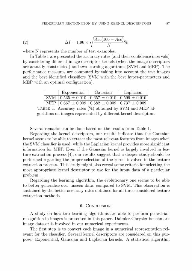
PEDESTRIAN RECOGNITION BY USING KERNEL DESCRIPTORS 87
(2) ∆I = 1.96×√Acc(100−Acc)
N%
where N represents the number of test examples.In Table 1 are presented the accuracy rates (and their confidence intervals)
by considering different image descriptor kernels (when the image descriptorsare actually constructed) and two learning algorithms (SVM and MEP). Theperformance measures are computed by taking into account the test imagesand the best identified classifiers (SVM with the best hyper-parameters andMEP with an optimal configuration).
Exponential Gaussian LaplacianSVM 0.535 ± 0.010 0.657 ± 0.010 0.599 ± 0.010MEP 0.667 ± 0.009 0.682 ± 0.009 0.737 ± 0.009
Table 1. Accuracy rates (%) obtained by SVM and MEP al-gorithms on images represented by different kernel descriptors.
Several remarks can be done based on the results from Table 1.Regarding the kernel descriptors, our results indicate that the Gaussian
kernel seems to be able to extract the most relevant features from images whenthe SVM classifier is used, while the Laplacian kernel provides more significantinformation for MEP. Even if the Gaussian kernel is largely involved in fea-ture extraction process [4], our results suggest that a deeper study should beperformed regarding the proper selection of the kernel involved in the featureextraction process. This study might also reveal some criteria for selecting themost appropriate kernel descriptor to use for the input data of a particularproblem.
Regarding the learning algorithm, the evolutionary one seems to be ableto better generalise over unseen data, compared to SVM. This observation issustained by the better accuracy rates obtained for all three considered featureextraction methods.
6. Conclusions
A study on how two learning algorithms are able to perform pedestrianrecognition in images is presented in this paper. Daimler-Chrysler benchmarkimage dataset is involved in our numerical experiments.
The first step is to convert each image in a numerical representation rel-evant for the classifier. Several kernel descriptors are considered on this pur-pose: Exponential, Gaussian and Laplacian kernels. A statistical algorithm

88 A. ANDREICA, L. DIOSAN, R. GACEANU, A. SIRBU
— SVM — and an evolutionary approach — MEP — are used for the learn-ing phase for which the input data is represented by the previously extractedfeatures.
Better accuracy rates are obtained when using the evolutionary model forall considered kernel descriptors. This might be considered an indicator of thesuperiority of the evolutionary approach over SVM for the considered problem.
Regarding the kernel descriptors used, SVM learning indicates that theGaussian is the best one, while MEP achieves the best results by using theLaplacian kernel. Therefore, we can not conclude which is the most efficientkernel descriptor and we intend to perform a further study of how the kernelselection influences the quality of recognition.
Our future work will also include a validation of the obtained results byconsidering other datasets like Caltech or INRIA.
References
[1] Alonso, I. P., Llorca, D. F., Sotelo, M. A., Bergasa, L. M., de Toro, P. R.,Nuevo, J., Ocana, M., and Garrido, M. A. G. Combination of feature extractionmethods for SVM pedestrian detection. IEEE Trans. Intelligent Transportation Systems8, 2 (Apr. 2007), 292–307.
[2] Bay, H., Tuytelaars, T., and Gool, L. J. V. SURF: Speeded up robust features.In ECCV (2006), pp. I: 404–417.
[3] Bo, L., Lai, K., Ren, X., and Fox, D. Object recognition with hierarchical kerneldescriptors. In CVPR (2011), IEEE, pp. 1729–1736.
[4] Bo, L., Ren, X., and Fox, D. Kernel descriptors for visual recognition. In NIPS(2010), J. D. Lafferty, C. K. I. Williams, J. Shawe-Taylor, R. S. Zemel, and A. Culotta,Eds., Curran Associates, Inc, pp. 244–252.
[5] Boser, B. E., Guyon, I., and Vapnik, V. A training algorithm for optimal marginclassifiers. In COLT (1992), D. Haussler, Ed., ACM Press, pp. 144–152.
[6] Chang, C.-C., and Lin, C.-J. LIBSVM: a library for support vector machines, 2001.Software available at http://www.csie.ntu.edu.tw/~cjlin/libsvm.
[7] Dalal, N., and Triggs, B. Histograms of Oriented Gradients for human detection.In CVPR (2005), C. Schmid, S. Soatto, and C. Tomasi, Eds., vol. 2, pp. 886–893.
[8] Dalal, N., Triggs, B., and Schmid, C. Human detection using oriented histogramsof flow and appearance. In ECCV (2006), pp. II: 428–441.
[9] Diosan, L., and Rogozan, A. How the kernels can influence image classificationperformance. Studia Universitatis Babes-Bolyai : Series Informatica LVII, 4 (2012),97–109.
[10] Espejo, P., Ventura, S., and Herrera, F. A survey on the application of geneticprogramming to classification. Transactions on Systems, Man ans Cybernetic, Part C40 (2010), 121–144.
[11] Grosan, C., and Abraham, A. Intelligent systems: A modern approach. New York,Springer, 2011.
[12] Koza, J. R. Genetic Programming: On the Programming of Computers by Means ofNatural Selection. MIT Press, 1992.

PEDESTRIAN RECOGNITION BY USING KERNEL DESCRIPTORS 89
[13] Lampert, C. Kernel methods in computer vision. presentation during Computer Visionand Sports Summer School, Prague, 2012, 2012.
[14] Lowe, D. G. Distinctive image features from scale-invariant keypoints. InternationalJournal of Computer Vision 60, 2 (2004), 91–110.
[15] Munder, S., and Gavrila, D. M. An experimental study on pedestrian classification.IEEE Trans. Pattern Analysis and Machine Intelligence 28, 11 (Nov. 2006), 1863–1868.
[16] Oltean, M. Improving the search by encoding multiple solutions in a chromosome.In Evolutionary Machine Design: Methodology and Applications, N. Nedjah and L. deMacedo Mourelle, Eds. Nova Publishers, 2005, ch. 4, pp. 85–110.
[17] Paisitkriangkrai, S., Shen, C. H., and Zhang, J. Fast pedestrian detection usinga cascade of boosted covariance features. IEEE Trans. Circuits and Systems for VideoTechnology 18, 8 (Aug. 2008), 1140–1151.
[18] Platt, J. Fast training of Support Vector Machines using Sequential Minimal Opti-mization. In Advances in Kernel Methods — Support Vector Learning (Cambridge, MA,1999), B. Scholkopf, C. J. C. Burges, and A. J. Smola, Eds., MIT Press, pp. 185–208.
[19] Scholkopf, B. The kernel trick for distances. In NIPS (Cambridge, MA, 2000), T. K.Leen, T. G. Dietterich, and V. Tresp, Eds., MIT Press, pp. 301–307.
[20] Vapnik, V. The Nature of Statistical Learning Theory. Springer, 1995.[21] Vapnik, V. Statistical Learning Theory. Wiley, 1998.[22] Viola, P., and Jones, M. Rapid object detection using a boosted cascade of simple
features. Proc. CVPR 1 (2001), 511–518.[23] Walk, S., Majer, N., Schindler, K., and Schiele, B. New features and insights
for pedestrian detection. In CVPR (2010), IEEE, pp. 1030–1037.[24] Zhao, L., and Thorpe, C. E. Stereo- and neural network-based pedestrian detection.
IEEE Transactions on Intelligent Transportation Systems 1, 3 (2000), 148–154.
(1) Babes-Bolyai University, Department of Computer Science, Cluj-Napoca,Romania
E-mail address: {anca,lauras,radu,adela}@cs.ubbcluj.ro
STUDIA UNIV. BABES–BOLYAI, INFORMATICA, Volume LVIII, Number 2, 2013
A COMPARISON OF REINFORCEMENT LEARNING BASED
MODELS FOR THE DNA FRAGMENT ASSEMBLY
PROBLEM
GABRIELA CZIBULA, ISTVAN-GERGELY CZIBULA, AND IULIANA M. BOCICOR(1)
Abstract. The DNA fragment assembly is a very complex optimiza-tion problem important within many fields, such as bioinformatics, com-putational biology or medicine. The problem is NP-hard, that is whymany computational techniques, including computational intelligence al-gorithms, were designed to find good solutions for this problem. Thispaper is intended to present and investigate two reinforcement learningbased models for solving the DNA fragment assembly problem. We pro-vide an experimental comparison of these two models, that will study theobtained performances of the reinforcement learning based approaches, byusing different action selection policies, with variable parameters.
1. Introduction
Determining the order of nucleotide bases, or the process of DNA sequenc-ing, has nowadays become of great importance in basic biology research, aswell as in various fields such as medicine, biotechnology or forensic biology.The main problem with the current sequencing technology is that it cannotread an entire genome at once, not even more than 1000 nucleobases.
The DNA fragment assembly (FA) refers to reconstructing the originalDNA sequence from a large number of fragments, each several hundred nucle-obases long, based on common subsequences of fragments. It is an NP-hardcombinatorial optimization problem, growing in importance and complexityas more research centers become involved in sequencing new genomes [5].
Received by the editors: April 12, 2013.2010 Mathematics Subject Classification. 68P15, 68T05.1998 CR Categories and Descriptors. I.2.6[Computing Methodologies]: Artificial In-
telligence – Learning ; I.2.8[Computing Methodologies]: Problem Solving, Control Meth-ods, and Search – Heuristic methods.
Key words and phrases. Bioinformatics, DNA fragment assembly, reinforcement learning,Q-learning.
This paper has been presented at the International Conference KEPT2013: KnowledgeEngineering Principles and Techniques, organized by Babes-Bolyai University, Cluj-Napoca,July 5-7 2013.
90

A COMPARISON OF RL MODELS FOR THE FRAGMENT ASSEMBLY PROBLEM 91
Reinforcement Learning (RL) [14] is an approach to machine intelligencein which an agent [13] can learn to behave in a certain way by receivingpunishments or rewards for its chosen actions. The learner is not told whichactions to take, as in most forms of machine learning, but instead must discoverwhich actions yield the highest reward by trying them.
In this paper we aim at investigating two reinforcement learning basedmodels for solving the problem of DNA fragment assembly. One of these mod-els, which was previously proposed in [2], is improved in this study. Moreover,this paper introduces a second reinforcement learning based model for thesame problem and compares the two approaches.
The rest of the paper is organized as follows. Section 2 introduces theDNA fragment assembly problem as well as some main aspects related to re-inforcement learning. The reinforcement learning models that we propose forsolving the FA problem are detailed in Section 3. Experimental evaluations,analysis and comparisons of the algorithms are given in Section 4. Section 5outlines some conclusions of the paper and indicates future research directions.
2. Background
This section briefly presents the DNA FA problem as well as some funda-mental aspects related to reinforcement learning.
2.1. The DNA Fragment Assembly Problem. Determining the order ofnucleotide bases (molecules composing the DNA), or the process of DNA se-quencing, has nowadays become of great importance in basic biology research,as well as in fields such as medicine, biotechnology or forensic biology. Themain problem with the current sequencing technology is that it cannot read anentire genome at once, not even more than 1000 bases. As even the simplestorganisms (such as viruses or bacteria) have much longer genomes, the needto develop methods that would overcome this limitation arose. One of these,called shotgun sequencing was introduced in 1982, by Fred Sanger [11] and itconsists of the next steps: first, several copies of the DNA molecule are cre-ated; then each of the copies is cut at random sites in order to obtain moleculesshort enough to be sequenced directly - fragments; the last and most difficultstep involves assembling these molecules back into the original DNA, based oncommon subsequences of fragments. The DNA FA problem specifically refersto this last step. For more details, we refer the reader to [2].
2.2. Reinforcement Learning. Background. Reinforcement Learning [8]is an approach to machine intelligence that combines two disciplines to solvesuccessfully problems that neither discipline can address individually: Dy-namic programming and Supervised learning. RL is a synonym of learning by

92 GABRIELA CZIBULA, JSTVAN-GERGELY CZIBULA AND IULIANA M. BOCICOR
interaction [10]. During learning, the adaptive system tries some actions (i.e.,output values) on its environment, then, it is reinforced by receiving a scalarevaluation (the reward) of its actions. The reinforcement learning algorithmsselectively retain the outputs that maximize the received reward over time.Reinforcement learning tasks are generally treated in discrete time steps. InRL, the computer is simply given a goal to achieve. The computer then learnshow to achieve that goal by trial-and-error interactions with its environment.
An important aspect in reinforcement learning is maintaining an equilib-rium between exploitation and exploration [15]. The agent should accumulatea lot of reward, by choosing the best experienced actions, but at the sametime it must explore its environment, by trying new actions. In this study weuse three policies for selecting actions: the ε-greedy policy [14], the softmaxpolicy [14] and an intelligent ε-Greedy based action selection mechanism, thatwe have introduced in [3], which uses a one step look-ahead procedure in orderto better guide the exploration of the agent through the search space.
3. Reinforcement Learning Based Models for the DNAFragment Assembly Problem
In this section we introduce the two reinforcement learning models pro-posed for solving the DNA FA problem. First, we present some concepts andnotations that will apply to both models.
A general reinforcement learning task is characterized by four components:a state space S specifying all possible configurations of the system; an actionspace A listing all available actions for the learning agent; a transition functionδ specifying the possibly stochastic outcomes of taking each action in any state;a reward function defining the possible reward of taking each of the actions.
Let us consider that Seq is a DNA sequence and F1, F2, . . . , Fn is a set offragments. As indicated in Subsection 2.1, the FA problem consists of deter-mining the order in which these fragments have to be assembled back into theoriginal DNA molecule, based on common subsequences of fragments. Conse-quently, the FA problem can be viewed, from a computational perspective, asthe problem of generating a permutation σ of {1, 2, . . . , n} that optimizes theperformance of the alignment Fσ = (Fσ1 , Fσ2 , . . . , Fσn) (n > 1). The perfor-mance measure PM we consider in this paper is one of the fitness functionsdefined in [9], which sums the overlap scores over all adjacent fragments andhas to be maximized. According to [9], the performance measure PM for thesequence of fragments Fσ = (Fσ1 , Fσ2 , . . . , Fσn) is defined as in Equation (1):
(1) PM(Fσ) =
n−1∑i=1
w(Fσi , Fσi+1)

A COMPARISON OF RL MODELS FOR THE FRAGMENT ASSEMBLY PROBLEM 93
where w(a, b) denotes the similarity measure between sequences a and b.
3.1. Path Finding Model. We have previously introduced a reinforcementlearning based model for the FA problem [2]. In the rest of the paper, it willbe referred to as the path finding model. The RL task associated to the FAproblem consists in training the agent to find a path from the initial to a finalstate having the maximum associated overall similarity. During the trainingstep of the learning process the learning agent determines its optimal policy inthe environment, i.e. the mapping from states to actions that maximizes thesum of the received rewards. The equivalent action configuration is viewed asa permutation that gives the optimal alignment of the DNA fragments. As thegoal is to find a path having the maximum value of the performance measure,the reinforcement function rewards the agent with a small value (e.g. 0.1) foreach transition to an non terminal state and with the performance measure ofthe found alignment, after a transition to a final state [2]. For training the FAagent [2] we used a Q-learning approach [14], in conjunction with an ε-Greedyaction selection policy. For more details about the definitions of the state andaction spaces or reward and transition functions, we refer the reader to [2].
Here we propose a modification of the reward function for this model, inorder to better guide the agent towards good solutions. The reward function,as defined in [2], illustrates situations when feedback is given at the end of eachtrial episode. It will be modified so as to give feedback to the agent after eachtransition to a new state, even if the state is not final. The moment of reward-ing is important in the learning process, as learning happens faster if feedbackis being given after each transition from one state to another. If we denote byπ a path from the initial to a final state, π = (π0π1π2 . . . πn), where π0 = s1(s1 is the initial state), by aπ = (aπ0aπ1aπ2 . . . aπn−1) - the sequence of actionsobtained following the transitions between the successive states from the pathπ, which gives the alignment of fragments Faπ = (Faπ0 , Faπ1 , . . . , Faπn−1
) (see
[2]), then the new definition of the reward function is given in Formula 2:
(2) r(πk|s1, π1, π2, . . . , πk−1) =
{0 if k = 1w(Faπk−1
, Faπk−2) otherwise
where by r(πk|s1, π1, π2, . . . , πk−1) we denote the reward received by the agentin state πk, after its history in the environment is π = (π0 = s1, π1, π2, . . . , πk−1).
Therefore, after each transition to a new state, the FA agent receives asreward the value of the similarity measure between the fragment correspondingto the current action and the fragment corresponding to the previously takenaction. As the learning goal is to maximize the total amount of rewardsreceived on a path from the initial to a final state, the FA agent is actually

94 GABRIELA CZIBULA, JSTVAN-GERGELY CZIBULA AND IULIANA M. BOCICOR
trained to find a path π that maximizes the overall similarity of the associatedalignment.
3.2. Permutation Model. In the following, we introduce a second reinforce-ment learning based model for the DNA FA problem, considering the generalaspects introduced at the beginning of this section. In the rest of the paper,this model will be referred to as the permutation model.
The components of the reinforcement learning task are:
• The state space S (the agent’s environment) will consist of n! states,i.e S = {s1, s2, . . . , sn!}. Each state si, i = 1, n! in the environmentwill represent a permutation of all the elements from the fragment set{F1, F2, . . . , Fn} : Fσi = (Fσi1
, Fσi2, . . . , Fσin). The initial state will be
represented by the identical permutation s0 = (F1, F2, . . . , Fn). A states reached by the agent at a given moment will be considered a terminal(final) state if the associated performance measure is sufficiently closeto a goal value. However, in order to be able to define a final state,apriori knowledge is needed to determine an upper bound of the set ofvalues for the performance measure of all possible permutations.
• The action space consists of(n2
)= n(n−1)
2 actions available to the prob-
lem solving agent. Let us denote byNa = n(n−1)2 the number of actions.
An action will be a pair of distinct indices (i, j), i, j ∈ {1, · · · , n}, i 6= jspecifying that the fragments located at indices i and j in the cur-rent state will be interchanged in order to make a transition to thefollowing state. Therefore, the action space may be represented asA = {a1, a2, . . . , aNa}, where ak ∈ {(i, j)|i, j ∈ {1, · · · , n}, i 6= j}, ∀1 ≤k ≤ Na.• The transition function δ : S → P(S) between the states is defined as:
(3) δ(sj) =
Na⋃k=1
∆(sj , ak) ∀j ∈ {1, · · · , n!},
where ∆(sj , ak) = sl, ∀j, l ∈ {1, · · · , n!}, l 6= j and sl is the stateresulted from sj , by interchanging the elements on the positions spec-ified by ak. This means that, at a given moment, from a state s ∈ Sthe agent can move in Na successor states, by executing one of the Na
possible actions. The transitions between the states are equiprobable,the transition probability P (s, s′) between a state s and each neighborstate s′ of s is equal to 1/Na.• The reward function will also be based on the performance measure for
a sequence of fragments, as defined in Formula (1). In this case, the
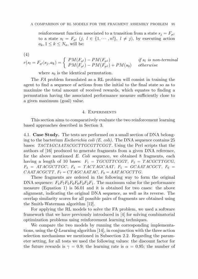
A COMPARISON OF RL MODELS FOR THE FRAGMENT ASSEMBLY PROBLEM 95
reinforcement function associated to a transition from a state sj = Fσjto a state sl = Fσl (j, l ∈ {1, · · · , n!}, l 6= j), by executing actionak, 1 ≤ k ≤ Na, will be:
(4)
r(sl = Fσl |sj , ak) =
{PM(Fσl)− PM(Fσj ) if sl is non-terminalPM(Fσl)− PM(Fσj ) + PM(s0) otherwise
where s0 is the identical permutation.
The FA problem formulated as a RL problem will consist in training theagent to find a sequence of actions from the initial to the final state so as tomaximize the total amount of received rewards, which equates to finding apermutation having the associated performance measure sufficiently close toa given maximum (goal) value.
4. Experiments
This section aims to comparatively evaluate the two reinforcement learningbased approaches described in Section 3.
4.1. Case Study. The tests are performed on a small section of DNA belong-ing to the bacterium Escherichia coli (E. coli). The DNA sequence contains 25bases: TACTAGCAATACGCTTGCGTTCGGT . Using the Perl scripts that theauthors of [16] produced to generate fragments from a given DNA reference,for the above mentioned E. Coli sequence, we obtained 8 fragments, eachhaving a length of 10 bases: F1 = TGCGTTCGGT , F2 = TACGCTTGCG,
F3 = ATACGCTTGC, F4 = TACTAGCAAT , F5 = GCAATACGCT , F6 =
CAATACGCTT , F7 = CTAGCAATAC, F8 = AATACGCTTG.These fragments are ordered in the following way to form the original
DNA sequence: F4F7F5F6F8F3F2F1. The maximum value for the performancemeasure (Equation 1) is 56.01 and it is obtained for two cases: the abovealignment, indicating the original DNA sequence, as well as its reverse. Theoverlap similarity scores for all possible pairs of fragments are obtained usingthe Smith-Waterman algorithm [12].
For applying the RL models to solve the FA problem, we used a softwareframework that we have previously introduced in [4] for solving combinatorialoptimization problems using reinforcement learning techniques.
We compare the two models by running the corresponding implementa-tions, using theQ-Learning algorithm [14], in conjunction with the three actionselection mechanisms we mentioned in Subsection 2.2. Regarding the param-eter setting, for all tests we used the following values: the discount factor forthe future rewards is γ = 0.9; the learning rate is α = 0.95; the number of

96 GABRIELA CZIBULA, JSTVAN-GERGELY CZIBULA AND IULIANA M. BOCICOR
training episodes is 4 · 105. In the case of the permutation model, the maxi-mum value of the performance measure was defined to be 57 and a state wasconsidered final if its performance measure was at most 1 unit away from thismaximum. For each of the three action selection policies, tests were made fordifferent values of the policy parameter (ε - in the case of ε-greedy and the onestep look-ahead procedure and τ - in the case of softmax): {0.2, 0.4, 0.6, 0.8}.Each algorithm was run five times, for each case of selection policy and eachvalue of the policy parameter and the shown results are averaged over theseruns. We mention that the experiments were carried out on a PC with anIntel Core i3 Processor at 2.4 GHz, with 3 GB of RAM.
4.2. Comparative Results. Below we present the results obtained by theQ-learning based algorithms implementing the models described in Section 3.
The path finding model proves to obtain the correct alignment of frag-ments with all three action selection mechanisms, the difference being thenumber of training epochs needed to converge to the optimal solution. Theleft-hand side of Figure 1 illustrates the performance measure of the solutionsobtained during the training process. For all three action selection policies,the algorithm converges to the optimal solution, the one having a performancemeasure of 56.01. We note that the algorithm using the one step look-aheadprocedure achieves the fastest convergence, reaching the correct solution afteronly 103 training epochs, for ε = 0.8. The next best, in terms of trainingepochs until convergence, is the algorithm using the softmax policy, the lastone being the ε-greedy algorithm. In all three cases, as the values of the policyparameter increase, thus leading to more exploration of the states space, theconvergence is achieved more rapidly: on average, for ε = 0.2 and τ = 0.2, thealgorithm converges (to the optimal or near-optimal solution) after 153 · 103
epochs, while for ε = 0.8 and τ = 0.8, the maximum performance measure isreached, on average, after only 25 · 103 epochs.
In terms of accuracy, the permutation model performs equally well, deter-mining the correct alignment for all the tests. In what concerns the number oftraining epochs, this second approach outperforms the first, for the case studywe considered. As can be seen on the right-hand side of Figure 1, the permu-tation model needs fewer epochs to reach the right solution: on average, for allthree action selection policies, convergence is reached after ∼ 6 ·103 epochs, asopposed to ∼ 84 ·103 epochs, which are needed on average for the path findingmodel. In this case, all three action selection policies find the solution equallyfast, but for different values of the policy parameter. Generally, as the valueof the policy parameter increases, the convergence is achieved sooner.
In the following, we will also offer an analysis of the computational timeneeded for the proposed RL algorithms in order to reach the correct solution.
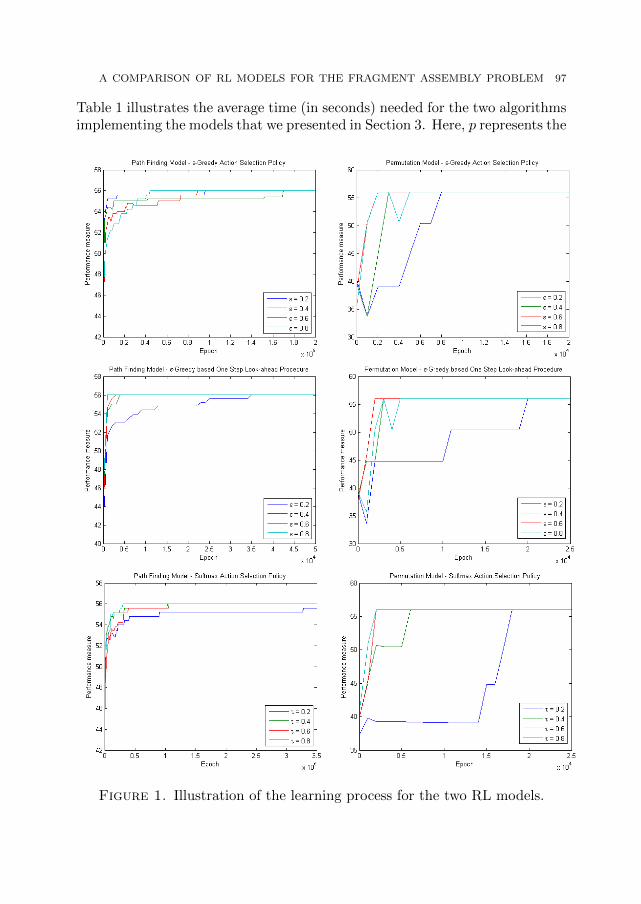
A COMPARISON OF RL MODELS FOR THE FRAGMENT ASSEMBLY PROBLEM 97
Table 1 illustrates the average time (in seconds) needed for the two algorithmsimplementing the models that we presented in Section 3. Here, p represents the
Figure 1. Illustration of the learning process for the two RL models.

98 GABRIELA CZIBULA, JSTVAN-GERGELY CZIBULA AND IULIANA M. BOCICOR
Path Finding Model Permutation Modelp = 0.2 p = 0.4 p = 0.6 p = 0.8 p = 0.2 p = 0.4 p = 0.6 p = 0.8
ε-Greedy policy 2.8 9.2 14.8 11.4 < 2 < 2 < 2 < 2
Look-ahead procedure 2.2 < 2 < 2 < 2 4 < 2 < 2 < 2
Softmax policy 29.6 17.4 40.6 10.2 705.8 44.6 35.6 26.8
Table 1. Average computational time (in seconds) needed foreach of the presented algorithms to reach the correct solution.
policy parameter, referring to ε, in the case of the ε-greedy based mechanismsand to τ , for the softmax action selection policy.
Even though intuitively the time is directly correlated with the numberof training epochs, between the two models there are some major differences,which lead to different durations for epochs. For instance, in the case of thepath finding model, the agent executes exactly 8 actions, to reach a finalconfiguration. For the permutation model, however, the number of actions isdifferent in each epoch, as the agent keeps trying actions until it reaches a statehaving a performance measure as close as possible to the maximum definedvalue. Hence, according to the way the agent explores the search space and theway it exploits existing knowledge, an epoch in the permutation model couldlast less or longer than one in the path finding model. From Table 1 we noticethat for the ε-greedy mechanism, the solution is reached in less time usingthe permutation model. Even if an epoch in the permutation model wouldlast longer, the number of epochs needed until convergence is more than 26times less than the number of epochs until convergence in the path findingapproach. Another important observation concerns the softmax policy. Anagent guiding its search by softmax must rank all the possible actions from astate, which requires extra computations that are not necessary for the othertwo policies. Therefore, as shown in Table 1, the algorithms using softmaxneed more time for each epoch, consequently more time, in total. Futhermore,regarding the permutation model, from any given state, there are 28 possibleactions (compared to only 8, for the other model) and then the computationsneeded for softmax take even longer, as can be seen from Table 1.
4.3. Discussion and Comparison to Related Work. We have experi-mented with two reinforcement learning based models, proposed for the prob-lem of DNA fragment assembly, used in conjuction with three different actionselection mechanisms: ε-greedy [14], an intelligent ε-Greedy based look-aheadaction selection mechanism that we have previously introduced [3] and thesoftmax selection policy [14]. The path finding model was introduced in adifferent study [2] and uses a Q-learning algorithm, with an ε-greedy action

A COMPARISON OF RL MODELS FOR THE FRAGMENT ASSEMBLY PROBLEM 99
selection policy. In this paper we have improved the path finding model andwe have introduced the permutation model, which is also based on Q-learning.
Both algorithms demonstrated to find the correct alignment of fragments,for the DNA sequence that we considered for the experiments. The differencebetween them lies in the number of training epochs and the computationaltime each one needs to achieve convergence.
For the considered case study and parameter setting, the permutationmodel proved to outperform the path finding approach, in all cases, wheninspecting the number of epochs. In what concerns the computational time,the situation is the same, for the ε-greedy policy, when the permutation basedalgorithm finds the correct solution in less than 2 seconds. Still, for the soft-max action selection policy, the required time is considerably higher. Weremark that in both cases, the algorithms using the intelligent action selectionprocedure [3] converge, on average, in less epochs than those using ε-greedyor softmax, as this procedure efficiently guides the exploration of the searchspace. We will further investigate how an intelligent action selection mecha-nism, based on softmax instead of ε-Greedy, could influence the outcome.
Regarding the permutation model, we note the following. As it is difficultto determine a final state, we need apriori information about the possiblevalues of the performance measure for permutations. Another option wouldbe to consider a state terminal if the number of actions that were performedfrom the initial state equals a given maximum number of steps. However, theproblem with this course of action could be the fact that the agent would notaim to maximize the total sum of rewards, but the sum of rewards obtainedafter the given number of maximum steps. A second observation concerns theaction space. In this study we use a fairly simple definition of an action, butfurther work will be done to investigate new types of actions, such as operatorsinspired from the field of genetic algorithms (e.g. crossover, mutation).
We remark that for the permutation model the number of states of theenvironment is smaller than for the path finding approach. However, an im-portant drawback of the permutation model is the fact that apriori knowledgeabout the problem is needed in order to define a final state and this infor-mation is not available in all types of situations. Therefore, the path findingapproach is more general and, as the results it obtains are good both in termsof accuracy and in terms of computational time, we conclude that it is better.
In the following, we will briefly compare our models with other approachesexisting in the literature for the FA problem. Since the used data sets are dif-ferent from one study to another, we cannot offer a very detailed comparison.
Kikuchi and Chakraborty [6] present an improved genetic algorithm toapproach the FA problem. To improve the efficiency of the simple geneticalgorithm (regarding both speed and solution quality), the authors introduce

100 GABRIELA CZIBULA, JSTVAN-GERGELY CZIBULA AND IULIANA M. BOCICOR
two new ideas, one of which implies manually combining fragments at certaingenerations. Compared to the approach from [6], our RL based methods donot need user intervention during the training process of the agent.
A comparison of four heuristic DNA FA algorithms is provided by Li andKhuri in [7]: a genetic algorithm, a greedy algorithm, a clustering heuristicalgorithm and one using structured pattern matching. All algorithms areexperimentally evaluated on several data sets, with the number of fragmentsranging from 39 to 773. The authors determined that the running times ofall four algorithms ranged from a few seconds to several hours. Even thoughthe data set we use contains a smaller number of fragments, the maximumamount of time needed by the RL approaches is less than 12 minutes, whilethe minimum is less than 2 seconds. Therefore, we believe that even for largerinstances it is likely that the necessary time for the RL models to converge tothe correct solution is of the order of minutes, rather than hours.
Angeleri et al. [1] introduce a supervised approach, based on a recurrentneural network to solve the FA problem. In the case of supervised models,a set of inputs with their target outputs is required. The advantage of ourRL methods is that the learning process needs no external supervision, as inour approach the solution is learned from the rewards obtained by the agentduring its training. Still, as mentioned before, the permutation model requiresapriori knowledge about the problem.
5. Conclusions and Further Work
In the present study we investigated two reinforcement learning basedmodels (the permutation model and the path finding model) for an importantproblem in bioinformatics, namely the DNA fragment assembly problem. Thealgorithms implementing both approaches, using three different action selec-tion policies, have been experimentally evaluated and compared.
We plan to extend the evaluation of both Q-learning based algorithmsfor larger DNA sequences, and implicitly greater number of fragments, tofurther develop the analysis. We will also investigate possible improvementsof these models by adding various local search mechanisms, by combining thesoftmax policy with the intelligent action selection procedure introduced in [3],by decreasing the action selection parameters (ε and τ) during the trainingprocess or by extending the permutation model to a distributed RL approach.
ACKNOWLEDGEMENT
This work was partially supported by the Sectoral Operational Programmefor Human Resources Development 2007-2013, co-financed by the European

A COMPARISON OF RL MODELS FOR THE FRAGMENT ASSEMBLY PROBLEM 101
Social Fund, under the project number POSDRU/107/1.5/S/76841 with thetitle Modern Doctoral Studies: Internationalization and Interdisciplinarity.
References
[1] E. Angeleri, B. Apolloni, D. de Falco, and L. Grandi. DNA fragment assemblyusing neural prediction techniques. Int. J. Neural Syst., 9(6):523–544, 1999.
[2] M. Bocicor, G. Czibula, and I. G. Czibula. A Reinforcement Learning Approachfor Solving the Fragment Assembly Problem. In Proceedings of the 3th Interna-tional Symposium on Symbolic and Numeric Algorithms for Scientific Computing(SYNASC ’11), pages 191–198. IEEE Computer Society, 2011.
[3] G. Czibula, I. M. Bocicor, and I. G. Czibula. Temporal Ordering of Cancer Mi-croarray Data through a Reinforcement Learning Based Approach. PLoS ONE,8(4):e60883, 2013.
[4] I. G. Czibula, G. Czibula, and M. I. Bocicor. A Software Framework for SolvingCombinatorial Optimization Tasks. Studia Universitatis “Babes-Bolyai”, Infor-matica, Special Issue, LVI(3):3–8, 2011.
[5] A. E. Hassanien, M. G. Milanova, T. G. Smolinski, and A. Abraham. Compu-tational intelligence in solving bioinformatics problems: Reviews, perspectives,and challenges. In Computational Intelligence in Biomedicine and Bioinformat-ics, pages 3–47. 2008.
[6] S. Kikuchi and G. Chakraborty. Heuristically tuned GA to solve genome fragmentassembly problem. IEEE CEC, pages 1491–1498, 2006.
[7] L. Li and S. Khuri. A comparison of DNA fragment assembly algorithms. In Proc.of the Int?l Conf. on Mathematics and Engineering Techniques in Medicine andBiological Sciences, pages 329–335. CSREA Press, 2004.
[8] L. J. Lin. Self-Improving Reactive Agents Based On Reinforcement Learning,Planning and Teaching. Machine Learning, 8:293–321, 1992.
[9] R. J. Parsons, S. Forrest, and C. Burks. Genetic algorithms, operators, and DNAfragment assembly. In Machine Learning, pages 11–33. Kluwer Academic Pub-lishers, 1995.
[10] A. Perez-Uribe. Introduction to reinforcement learning, 1998.http://lslwww.epfl.ch/∼anperez/RL/RL.html.
[11] F. Sanger, A. Coulson, G. Hong, l. D. Hil, and G. Petersen. Nucleotide sequenceof bacteriophage Lambda DNA. J. Molecular Biology, 162(4):729–773, 1982.
[12] T. Smith and M. Waterman. Identification of Common Molecular Subsequences.Journal of Molecular Biology, 147(1):195–197, 1981.
[13] I. Susnea, G. Vasiliu, A. Filipescu, and A. Radaschin. Virtual pheromones forreal-time control of autonomous mobile robots. Studies in Informatics and Con-trol, 18(3):233–240, 2009.
[14] R. S. Sutton and A. G. Barto. Reinforcement Learning: An Introduction. MITPress, 1998.
[15] S. Thrun. The Role of Exploration in Learning Control. In Handbook for Intelli-gent Control: Neural, Fuzzy and Adaptive Approaches. Van Nostrand Reinhold,Florence, Kentucky, 1992.
[16] W. Zhang, J. Chen, Y. Yang, Y. Tang, J. Shang, B. Shen, and I. K. Jordan.A practical comparison of de novo genome assembly software tools for next-generation sequencing technologies. PLoS ONE, 6(3):e17915, 2011.

102 GABRIELA CZIBULA, JSTVAN-GERGELY CZIBULA AND IULIANA M. BOCICOR
(1) Babes-Bolyai University, Department of Computer Science, Cluj-Napoca,Romania
E-mail address: {gabis, istvanc, iuliana}@cs.ubbcluj.ro

STUDIA UNIV. BABES–BOLYAI, INFORMATICA, Volume LVIII, Number 2, 2013
BUSINESS PROCESS MINING USING ITERATED LOCAL
SEARCH
DIANA CHINCES(1) AND IOAN SALOMIE(1)
Abstract. This paper introduces ILS Miner, a novel method for dis-covering process models from event logs using iterated local search. Acomparison between ILS Miner, GLS Miner and HeuristicMiner is pre-sented in this paper. GLS Miner was chosen because applies Guided LocalSearch for discovering process models from event logs, HeuristicMiner[10]being a legacy method in business process discovery. It is shown that ILSMiner can discover process models that correctly map to the event log.ILS Miner works with business processes represented as graphs, and thefinal discovered process is represented as a BPMN diagram.
1. Introduction
The work efficiency in large organizations is given by optimal process flowsthat are followed in the company. In some cases, these process flows are justdefined and followed by employees, but in most of the cases the process flows(models) need to be discovered. Nowadays, organizations use different man-agement systems that keep track of all the work being done, generating socalled event logs. The process model that is being followed in the organizationcan be discovered from these event logs using process mining algorithms.Figure 1 shows an overview of process mining. The event logs are generated bythe information system used in the company and are the input for the processdiscovery algorithms. Not all the information from the database is included inthe event logs. In [3] the following assumptions are defined: each event refersto an activity (well-defined step in the process), each event refers to a case (the
Received by the editors: April 13, 2013.2010 Mathematics Subject Classification. 68-00, 68M14, 68M01, 68N01, 68P10 .1998 CR Categories and Descriptors. K.4.3 [Organizational Impacts]: Reengineer-
ing ; K.4.3 [Organizational Impacts]: Automation; K.4.3 [Organizational Impacts]:Computer-supported collaborative work .
Key words and phrases. Guided Local Search, GLS Miner, Iterated Local Search, busi-ness process mining, event log, BPMN .
This paper has been presented at the International Conference KEPT2013: KnowledgeEngineering Principles and Techniques, organized by Babes-Bolyai University, Cluj-Napoca,July 5-7 2013.
103

104 DIANA CHINCES AND IOAN SALOMIE
process instance), each event has a performer, and events have a timestampand are totally ordered. Knowing this, an event can be defined as a tuple (c,a, p), where c is the case, a the activity and p the performer. The events beingordered in time, causal relations can be defined between the activities and theactors. Given two tuples (c, a1, p1) and (c, a2, p2) from the event logs, itresults that activity a1 that is performed by person p1 is followed by activitya2, which is performed by person p2. For applying Guided Local Search forprocess discovery the performer is not needed, the algorithm only makes useof the cases, the activities and their order.Three different perspectives of process mining were identified in [4]: the pro-
Figure 1. Overview of process mining[2]
cess perspective, the organizational perspective and the case perspective. Theprocess perspective deals with discovering the process models from the eventlogs. Areas of applicability of the process perspective include IT managementprocesses governing the operations of services and infrastructure as well asscientific computing workflows. This process model can be further used asinput for applying optimization algorithms for improving the workflows in theorganization. The organization perspective focuses on the relations betweenthe individuals in the company and the case perspective mines the propertiesof the cases in the process. An important property of a case is the data at-tached to it. For example, if a case represents submitting an order it wouldbe interesting to have knowledge of the products ordered, the quantity, pricespaid, discounts etc.This paper aims at presenting a novel method for discovering process modelsfrom event logs using Iterated Local Search, focusing on the process perspec-tive.The remainder of the paper is organized as follows. Section 2 presents thebackground of process mining and related work. Section 3 explains the Iter-ated Local Search algorithm. Section 4 describes how Iterated Local Searchis used for process discovery, followed by Section 5 where the experiments

BUSINESS PROCESS MINING USING ITERATED LOCAL SEACH 105
of applying ILS Miner in process discovery are presented. In Section 6 theconclusions of this paper are stated.
2. Background and related work
This section reviews the state of the art in business process discovery anddescribes a common structure used for storing event logs for process mining.The information systems presented in Figure 1 use different data structuresto store the data. In [5] a generic framework for process discovery algorithmsand a common structure to be used were introduced. The ProM frameworkallows the creation of plugins for the process mining algorithms. The inputfor a plugin is an XML file in the MXML format [5]. Tools like Open Xes [6]allow the mapping and conversion between different log storing structures andMXML files.
Process mining algorithms, such as the Alpha algorithm [8] assume thatit is possible to sequentially order events, such that each event refers to a caseand an activity. The Alpha algorithm does not take into consideration thetimestamp of events. This information is used to automatically construct aprocess model, which in the Alpha algorithm is represented as a Petri Netdescribing the event logs.
Figure 2. The event log and the process model discovered byAlpha algorithm [9]
In Figure 2 a simple event log and the Petri-Net that was generated byapplying the Alpha algorithm can be observed. It can be noted from the figurethat the event log is easily reproduced from the discovered model.
The GLS Miner[14] is the first algorithm in which local search is appliedin the business process domain. It is shown in [14] that the GLS Miner cancorrectly discover heterogenous types of business processes. The search spacefor applying guided local search is a set of processes, represented as graphs.A process model is represented as a graph. The nodes of the graph representthe existent activities in the process model and the edges the flows betweenthe activities. The features necessary for guided local search were defined as

106 DIANA CHINCES AND IOAN SALOMIE
all possible edges in the graph. Thus, a solution has a feature available if andonly if the specific edge is available in the solution. The algorithm starts witha random graph and can either add or remove edges in order to move from asolution to another.
The HeuristicMiner [10] is a heuristic driven process mining algorithm,being considered one of the most relevant process discovery algorithms. It is apractical applicable mining algorithm that can deal with noise (e.g. exceptionsfrom the usual workflow that appear in the event log) and can be used toexpress the main behavior registered in an event log. The HeuristicMiner onlyconsiders the order of the events within a case by using the timestamp of theactivities. A log is defined in the same way as for the Alpha algorithm [9].The following log will be used for explaining the HeuristicMiner, W = [ABCD,ABCD, ACBD, ACBD, AED].
HeuristicMiner builds a dependency graph [10]. A frequency based metricis used to indicate how certain we are that there is truly a dependency relationbetween two events A and B:
a⇒W b =
(|a >W b| − |b >W a||a >W b|+ |b >W a|+ 1
)A high value of the ⇒W relation between a and b determines that there
is dependency relationship between a and b. Applying the heuristics to theevent log in Table 1 takes us to the results in Figure 3.
Figure 3. Dependency graph [10]
3. Iterated Local Search
Iterated local search can be easily explained as [12]: one iteratively buildsa sequence of solutions generated by the embedded heuristic, leading to better

BUSINESS PROCESS MINING USING ITERATED LOCAL SEACH 107
solutions than if one were to use repeated random trials of that heuristic.There are two main points that make an algorithm an iterated local search: (i)there must be a single chain that is being followed (thus excluding population-based algorithms); (ii) the search for better solutions occurs in a reduced spacedefined by the output of a blackbox heuristic.
A local search is a problem specific heuristic optimization algorithm. Inmost cases this algorithm can be improved iteratively, resulting in a iteratedlocal search algorithm. Algorithm 1 shows the generic iterated local searchalgorithm.
begins0 ← GenerateInitialSolution;
s∗ ← LocalSearch(s0);
while not termination criterion dos′ ← perturbation(s∗, history);
s′∗ ← LocalSearch(s′);
s∗ ← AcceptanceCriterion(s∗, s∗′, history);
end
endAlgorithm 1: Iterated Local Search Algorithm [12]
Iterated local search runs for each problem until the termination criteria ismet. The termination criteria has to be created for each particular problem.The iterated local search walk is not reversible. First, an initial solution isgenerated on which the search algorithm is applied. Until the terminationcriterion is met, the current best solution is perturbated and if it meets theacceptance criterion it may be used as the next best solution. A history ofperturbations can be included in the algorithm, so that the same perturbationis not applied several times on the same solution.
4. Iterated Local Search Miner
From the previous section presenting the general Iterated Local Searchalgorithm, we can conclude that for applying this for a specific problem, thefollowing items need to be defined:
• a termination criterion• a method for perturbation• an acceptance criterion

108 DIANA CHINCES AND IOAN SALOMIE
The search space for applying iterated local search is a set of processes,represented as graphs. The nodes of the graph represent the existing activ-ities in the process model while the edges the flows between the activities.Algorithm 2 shows the Iterated Local Search Miner (ILS Miner).
input : event log, maxIterationsoutput: process model mapped on the event logbegin
solution← random(log);
currentCost← computeCost(solution);
neighbor ← findNeighbor(solution);
k ← 0;
while neighbor 6= null and k < maxIterations dosolution← neighbor;
perturb(solution);
second← findNeighbor(solution);
currentCost← computeCost(solution);
secondCost← computeCost(second);
if secondCost ¡ currentCost thensolution← second
end
k ← k + 1;
end
returnsolution;
endAlgorithm 2: ILS Miner
We considered the termination criterion being the fact that the algorithmcannot find a better neighbor and the number of maximum iterations havebeen executed. Algorithm 3 shows the perturbation procedure.
input : graphoutput: graph’begin
edge← randomEdge();
graph.add(edge);return graph
endAlgorithm 3: Perturbation algorithm

BUSINESS PROCESS MINING USING ITERATED LOCAL SEACH 109
In the perturbation algorithm the graph is randomly modified. The algo-rithm perturbes the graph by adding a random edge to it. The perturbatedsolution and its neighbor is considered to pass the acceptance criterion if ithas a lower cost than the previous best solution. We have chosen to computehe cost as the sum of the frequency of edges in the graph. The frequency ofan edge (k,s) is computed based on the event log given as input to the miningalgorithm. The frequency of the occurrence (k,s) is computed as
(1)(number of occurrences of (k, s))
(number of occurences of (s, k) + 1)
5. Experiments and results
The Iterated Local Search BP Miner was implemented as a ProM Frame-work[5] plugin. This plugin was created for proof of concept of the algorithmdescribed in the previous section.
The results are presented as a comparison between the proposed Iter-ated Local Search BP Miner, the Guided Local Search BP Miner[14] and theHeuristic Miner[10]. This comparison is done considering the discovered pro-cess models and the errors encountered by each of the algorithms. Processmodels P1 (Figure 4), P2 (Figure 5) and P4 (Figure 6) were considered forthis comparison. P1 is a simple process model, having just a few flows fromthe start to the end activity. P2 is more complex, having alternative flowsfrom the start to the end activity. P3 has the most complexity as it containsloops. We considered for the experiments these three basic types of processesfor prove of concept. In the future, we plan to run scalability tests on thealgorithm using event logs from real data. Table 1 shows the event logs thatwere used for each process. The regularization value used for the experimentswas 0.6, however this is easily customizable in the ProM Framework plugin.
Figure 4. P1 - simple process model
Table 2 shows the comparison of the discovered process models by applyingthe ILS BP Miner and the GLS BP Miner. For process model P1 the ILS BPMiner, as well as the GLS Miner, have correctly discovered the model fromthe given event logs. We can observe that the Guided Local Search Miner hasdiscovered a process model that correctly maps to the event log, even if this

110 DIANA CHINCES AND IOAN SALOMIE
Figure 5. P2 - simple process model with alternative paths
Figure 6. P2 - process model with loops
is not the same with the initial process model. Applying a process miningalgorithm in an organization might end up with this kind of results, that theprocess model that is discovered from the event logs is not exactly the samewith the process model that was initially defined in the organization. Forprocess model P2 the both algorithms have correctly discovered the initialmodel, as shown from the error graph as well. For the last process model,the GLS Miner did not discover the entire model, but managed to obtain anearly correct process model. ILS Miner however discovered the a model whichcontains less errors than the model discovered by the GLS Miner.
Table 3 shows the comparison of the discovered process models by applyingthe ILS BP Miner and the Heuristic Miner[10]. For process model P1 the ILSBP Miner, as well as the GLS BP Miner, have correctly discovered the modelfrom te given event log. We can observe that for process model P2, ILS BPMiner has correctly discovered the process model, but the Heuristic Miner ismissing the edge from D to E. For the last process model, ILS BP Minerhas managed to obtain once again a model that is better than the HeuristicMiner. This can be observed also from Figure 6, showing the number of errorsencountered by each of the algorithms.
Figure 7 shows the number of errors encountered by each of the threealgorithms that were experimented.

BUSINESS PROCESS MINING USING ITERATED LOCAL SEACH 111
Traces for P1 Traces for P3Case Activity Time 1 A 19:00:00
1 A 19:00:00 B 19:01:00B 19:01:00 D 19:02:00D 19:02:00 F 19:03:00E 19:03:00 2 A 19:00:00
2 A 19:00:00 B 19:01:00C 19:01:00 E 19:02:00E 19:02:00 F 19:03:00
3 A 19:00:00 3 A 19:00:00B 19:01:00 C 19:01:00D 19:02:00 B 19:02:00E 19:03:00 E 19:03:00
Traces for P2 F 19:04:001 A 19:00:00 4 A 19:00:00
B 19:02:00 C 19:01:00C 19:03:00 E 19:02:00E 19:04:00 F 19:03:00
2 A 19:00:00 5 A 19:01:00B 19:01:00 B 19:02:00D 19:02:00 E 19:03:00C 19:03:00 A 19:04:00E 19:04:00 B 19:05:00
3 A 19:00:00 D 19:06:00B 19:01:00 F 19:07:00D 19:02:00 6 A 19:01:01E 19:03:00 C 19:02:00
B 19:03:00E 19:04:00F 19:05:00
Table 1. Traces considered for experiments
6. Conclusion
This paper introduced ILS Miner, a new algorithm for discovering processmodels from event logs. The experiments were done on heterogenous types ofprocesses and the results were compared with GLS Miner[14], another algo-rithm that applies local search for process discovery and HeuristicMiner[10],a legacy algorithm in process discovery. This paper shows that ILS Miner has

112 DIANA CHINCES AND IOAN SALOMIE
Processmodel
Initial process (known) ILS BP Miner GLS BP Miner
P1
P2
P3
Table 2. The initial (known) process model and the discov-ered models using ILS Miner and GLS Miner
Processmodel
Initial process (known) ILS BP Miner Heuristic Miner
P1
P2
P3
Table 3. The initial (known) process model and the discov-ered models using ILS Miner and Heuristic Miner
managed to correctly discover the process models from the event logs, showingthat the results are better than the ones obtained by both of GLS Miner andHeuristicMiner. In the future, we plan to apply our methods on more complexprocess models and on real data, comparing the results by the performance ofthe algorithms.

BUSINESS PROCESS MINING USING ITERATED LOCAL SEACH 113
Figure 7. Number of errors encountered by the algorithms
References
[1] Chris Voudouris, Edward Tsang, Guided Local search, Technical Report CSM–247, De-partament of Computer Science, University of Essex, August 1995
[2] A.K. Alves de Medeiros, A.J.M.M. Weijters and W.M.P. van der Aalst, Genetic ProcessMining An Experimental Approach, Data Mining and Knowledge Discovery Volume 14Number 2 (2007), pages 245-304
[3] W.M.P. van der Aalst, A.K.A. de Medeiros, Process Mining and Security: DetectingAnomalous Process Executions and Checking Process Conformance, Second InternationalWorkshop on Security Issues with Petri Nets and other Computational Models (WISP2004), pages 6984
[4] W.M.P van der Aalst, Business Alignment: Using Process Mining as a Tool for DeltaAnalysis and Conformance Testing, Requirements Engineering Volume 10 Number 3(2005), pages 198-211
[5] B.F. van Dongen and W.M.P. van der Aalst, A Generic Import Framework for ProcessEvent Logs, J. Eder and S. DUstdar, editors, Business Process Management Workshops,Workshop on Business Process Intelligence (BPI 2006), volume 4103 of Lecture Notes inComputer Science, pages 81-92
[6] Open Xes Homepage, http://xes-standard.org/openxes/start[7] Christos Voudouris, Edward Tsang, Guided Local Search and its application to the trav-
eling salesman problem, European Journal of Operational Research 113 (1999), pages469-499
[8] W.M.P. van der Aalst, A.J.M.M. Weijters, and L. Maruster. Workflow Mining: Dis-covering Process Models from Event Logs. IEEE Transactions on Knowledgeand DataEngineering, 16(9):11281142, 2004
[9] W.M.P. van der Aalst, V. Rubin, B.F. van Dongen, E. Kindler, and C.W. Gunther,Process Mining : A Two-Step Approach using Transition Systems and Regions, Softwareand System Modeling Volume 9 Number 1 (2010) pages 87-111

114 DIANA CHINCES AND IOAN SALOMIE
[10] A.J.M.M. Weijters, W.M.P. van der Aalst, and A.K. Alves de Medeiros, Process Miningwith the HeuristicsMiner Algorithm, BETA Working Paper Series, WP 166, EindhovenUniversity of Technology, Eindhoven
[11] W.M.P van der Aalst, Business Alignment: Using Process Mining as a Tool for DeltaAnalysis and Conformance Testing, Requirements Engineering Volume 10 Number 32005, pages 198-211
[12] Iterated Local Search, http://ideas.repec.org/p/upf/upfgen/513.html[13] Helena R. Lourenco, Olivier C. Martin, Thomas Stutzle, Iterated Local Search, Hand-
book of Metaheuristics, F. Glover and G. Kochenberger, Eds. International Series inOperations Research & Management Science, vol. 57. Kluwer Academic Publishers, Nor-well, MA, 321353
[14] Diana Chinces, Ioan Salomie, Business Process Mining using Guided Local Search, The12th International Symposium on Parallel and Distributed Computing - ISPDC 2013(accepted)
(1) Technical University Of Cluj-NapocaE-mail address: [email protected]
E-mail address: [email protected]

STUDIA UNIV. BABES–BOLYAI, INFORMATICA, Volume LVIII, Number 2, 2013
PLAYERS WITH UNEXPECTED BEHAVIOR: t-IMMUNE
STRATEGIES. AN EVOLUTIONARY APPROACH.
NOEMI GASKO(1), MIHAI SUCIU(1), RODICA IOANA LUNG(1),TUDOR DAN MIHOC(1), AND D. DUMITRESCU (1)
Abstract. An evolutionary detection method based on generative rela-tions for detecting the t-immune strategies of a non-cooperative game isintroduced. Numerical experiments on an economic game show the poten-tial of our approach.
1. Introduction
Game Theory (GT) offers proper models to characterize interactions be-tween agents with conflicting behaviours. The situations where divergent in-terests interact are modelled as mathematical games. Each player has a set ofstrategies (”moves”) that define his possible actions within the game. Manytypes of games have been proposed since the concept was first introduced:games with complete information (players have complete information on theentire game), cooperative or non-cooperative games (depending on the players’disposition to build unions or not), one shot games (players play one roundonly in the same time), etc.
One of GT’s main aim was to find patterns and solutions that will al-low scholars to accurate anticipate game’s outcomes and the behaviour of realplayers. An equilibrium concept designed for pure rational players, was intro-duced by Nash [8] and depicts that state where no individual player can gainmore by modifying his option within the game (his strategy) while the otherskeep theirs unchanged. Even if it is one of the central solution concepts in GT,Nash equilibrium was also criticized mostly because of the hard assumptionson players rationality [6]. Experiments conducted with real people lead to the
Received by the editors: April 15, 2013.2010 Mathematics Subject Classification. 91A10.1998 CR Categories and Descriptors. I.2.8 [Heuristic methods]: Artificial intelligence;Key words and phrases. non-cooperative games, t-immune strategy, evolutionary
detection.This paper has been presented at the International Conference KEPT2013: Knowledge
Engineering Principles and Techniques, organized by Babes-Bolyai University, Cluj-Napoca,July 5-7 2013.
115

116 GASKO, SUCIU, LUNG, MIHOC, AND DUMITRESCU
conclusion that Nash equilibrium is seldom the output for games with realplayers.
The search for more realistic models for real players leaded to entire classesof equilibria. The scholars tried to incorporate the ”human” factor in thesemodels but, even if at some point they succeeded at this task, the proper toolsto solve them were missing. Evolutionary computation can offer a solution forthis. The recent development of fitness solutions for game equilibria detection[5], [4] allows specialized techniques on strategic games to be developed.
In this study we present a tool, based on evolutionary computation, de-signed to detect a good approximation of a game t-immune equilibria. Thisequilibria attempts to capture the situations where agents are acting in anunpredictable manner, an irrational behaviour outlined by most of the exper-iments with real people.
The paper is organized in four sections: an introduction that presentsthe domain and emphasise the importance of the approached problem; in thesecond section the proposed technique is presented; the conducted numericalexperiments that validate the method are depicted in section three followedby the conclusions and further work section.
2. Evolutionary equilibrium detection for t-immune equilibriamodels
In order to detect the t-immune equilibrium for noncooperative gamesin strategic form a generative relation is introduced. Using this relation afitness measure is constructed and two evolutionary methods are modifiedand adapted to detect t-immune equilibria.
2.1. Prerequisites. A finite strategic game is a system G = ((N,Si, ui), i =1, ..., n), where:
• N represents a set of players, and n is the number of players;• for each player i ∈ N , Si is the set of actions available,
S = S1 × S2 × ...× Sn
is the set of all possible situations of the game.Each s ∈ S is a strategy (or strategy profile) of the game;
• for each player i ∈ N , ui : S → R represents the payoff function of i.
The most used solution concept in Game Theory is the Nash equilibrium[8]. Playing in Nash sense means that no one from the players can changeher/his strategy in order to increase her/his payoff while the others keep theirsunchanged.
t-immune equilibrium [1] models situations where players act unpredictable,not in a rational or expected way. A strategy is t-immune when less than t

t-IMMUNE STRATEGIES. AN EVOLUTIONARY APPROACH. 117
players change their strategy, but without affecting the payoffs for the otherplayers.
Definition 1. A strategy s∗ ∈ S is t-immune if, for all T ⊆ N , with card(T ) ≤t, all sT ∈ ST , and all i ∈ T :
ui(s∗−T , sT ) ≥ ui(s
∗).
t-immune equilibria models the tolerance threshold of players, how manyplayers can behave unpredictable without affecting the other players payoffs.
2.2. Generative relations. In order to compute equilibria we characterizethem with adequate relations on the strategy set. Such relations are calledgenerative relations of the equilibrium.
We have the quality measure:
Q : S × S → N,where S is the set of the strategy profiles.Let s and s∗ be two strategy profiles, s, s∗ ∈ S.In this case Q(s, s∗) measures the quality of strategy s with respect to the
strategy s∗.The quality Q is used to define the relation ≺Q:
s ≺Q s∗, if and only if Q(s, s∗) ≤ Q(s∗, s).
The first generative relation for the Nash equilibrium has been introducedin [7].
2.2.1. Generative relation for t-immune strategies. Consider a quality measuret(s∗, s), which denotes the number of players who gain by switching from onestrategy to the other strategies:
t(s∗, s) = card[i ∈ N − T, ui(sT , s∗−T ) ≤ ui(s
∗), sT = s∗T , card(T ) = t, T ⊆ N ],
where card[M ] represents the cardinality of the set M .
Definition 2. Let s∗, s ∈ S. We say the strategy s∗ is better than strategy swith respect to t-immunity, and we write s∗ ≺T s, if the following inequalityholds:
t(s∗, s) < t(s, s∗).
Definition 3. The strategy profile s∗ ∈ S is called t-immune non-dominated,if and only if there is no strategy s ∈ S, s = s∗ such that
s ≺T s∗.

118 GASKO, SUCIU, LUNG, MIHOC, AND DUMITRESCU
Table 1. Parameter settings for t-DE
Parameter ValuePop size 100Max no FFE 5000-2 players; 200000-3 playersCr 0.8F 0.3
The relation ≺T can be considered as the generative relation for t-immuneequilibrium, i.e. the set of non-dominated strategies, with respect to ≺T ,induces the t-immune strategies.
2.3. Evolutionary detection method. Two evolutionary algorithms areadapted for detecting t-immune equilibrium: NSGA-II (Non-dominated Sort-ing Genetic Algorithm II)[9] and DE (Differential Evolution) [10].
In both algorithms the Pareto dominance relation is replaced with thegenerative relation ≺T and two new evolutionary methods for t-immune equi-librium detection, called t-NSGA-II, respectively t-DE are obtained.
3. Numerical experiments - the Cournot game
In the normal Cournot model [3] n companies produce qi, i = 1, ..., nquantities of a homogeneous product.
Q =∑
i=1,n qi is the aggregate quantity on the market, a is a constant,
and the market clearing price is P (Q) = a−Q if Q < a and 0 otherwise.The total cost for company i for producing quantity qi is Ci(qi) = cqi. The
marginal cost c is constant, and c < a.The payoff for the company i can described as follows:
ui(q) = qiP (Q)− Ciqi,
where q = (q1, ..., qn). The final form of the payoff function can be describedas:
ui(q) = qi[a−∑j=1,n
qj − c], i = 1, ..., n.
In our experiments we consider a = 50, c = 10, qi ∈ [0, 10], i = 1, ..., n andthe two- and three player version of the Cournot game.
Parameter settings for t-DE are presented in Table 1. Parameter settingsfor t-NSGA-II are presented in Table 2. Ten different runs are considered, andthe mean and standard deviation is reported.
Result for the two players variant of the Cournot game are presented inTable 3. Table 4 depicts the three player version of the Cournot game, fort = {1, 2}.

t-IMMUNE STRATEGIES. AN EVOLUTIONARY APPROACH. 119
20
40
60
80
100
120
140
160
180
200
player 1 Payoff player 1 Strategy player 2 Payoff player 2 Strategy
Figure 1. Strategies and payoffs for the two player version ofthe Cournot game
10
20
30
40
50
60
70
80
90
100
p_1 Payoff p_1 Strategy p_2 Payoff p_2 Strategy p_3 Payoff p_3 Strategy
Figure 2. Detected 1-immune strategies and payoffs for thethree player version of the Cournot game

120 GASKO, SUCIU, LUNG, MIHOC, AND DUMITRESCU
Table 2. Parameter settings for t-NSGA-II
Parameter ValuePop size 100Max no FFE 5000-2 players; 185108-3 playersprob. of crossover 0.2prob. of mutation 0.2
Table 3. Results for 2 player Cournot game for 1-immuneequilibrium (mean values for 10 different runs).
Algorithm timmuneStrategy Payoffs1 s2 u1 u2
t-DE 1 10 10 200 200t-NSGA2 1 10 10 200 200
Table 4. Results for 3 player Cournot game for timmune ∈{1, 2} (mean values for 10 different runs).
Algorithm timmuneStrategy Payoff
s1 s2 s3 u1 u2 u3
t-DE1 10 10 10 100 100 1002 10 10 10 100 100 100
t-NSGA21 10 10 10 100 100 1002 10 10 10 100 100 100
Figures 1, 2 and 3 depict the t-immune equilibria for two and three players.Numerical experiments indicate that the players’ threshold is minimal in
both cases. The firms need to produce maximal quantity of products in orderto avoid the unexpected behavior of some firms.
4. Conclusions and further work
In this study a generative relation for the t-immune equilibrium is pro-posed. This generative relation is used in two different evolutionary algorithmsto guide the search towards desired equilibria. The Cournot oligopoly model -an economic game, is considered for numerical experiments. Results underlinethe stability and the potential of the proposed method.
Further experiments will focus on large games.

t-IMMUNE STRATEGIES. AN EVOLUTIONARY APPROACH. 121
10
20
30
40
50
60
70
80
90
100
p_1 Payoff p_1 Strategy p_2 Payoff p_2 Strategy p_3 Payoff p_3 Strategy
Figure 3. Detected 2-immune strategies and payoffs for thethree player version of the Cournot game
5. Acknowledgment
This project was supported by the national project code TE 252 and320 financed by the Romanian Ministry of Education and Research CNCSIS-UEFISCSU.
References
[1] Abraham, I., Dolev, D. Gonen, R., Halpern, J.: Distributed computing meets game theory:robust mechanisms for rational secret sharing and multiparty computation, Proceedings ofthe twenty-fifth annual ACM symposium on Principles of distributed computing, 53-62,2006.
[2] Basu, K.: The Traveler’s Dilemma: Paradoxes of Rationality in Game Theory, AmericanEconomic Review, 84:2, 391-395, 1994.
[3] Cournot, A.: Researches into the Mathematical Principles of the Theory of Wealth, NewYork: Macmillan, 1897.
[4] Dumitrescu, D., Lung, R. I., Mihoc, T. D.: Evolutionary Equilibria Detection in Non-cooperative Games, EvoStar2009, Applications of Evolutionary Computing, LectureNotes in Computer Science, Springer Berlin / Heidelberg, vol. 5484, 253-262, 2009.
[5] Dumitrescu, D., Lung, R. I., Mihoc, T. D.: Generative Relations for Evolutionary Equi-libria Detection, Proceedings of the 11th Annual conference on Genetic and EvolutionaryComputation, 1507-1512, 2009.
[6] Halpern, J.Y., Beyond Nash Equilibrium: Solutions Concepts for the 21th Century, Pro-ceedings of the twenty-seventh ACM symposium on Principles of distributed computing,1-10, 2008.

122 GASKO, SUCIU, LUNG, MIHOC, AND DUMITRESCU
[7] Lung, R. I., Dumitrescu, D.: Computing Nash Equilibria by Means of Evolutionary Com-putation, International Journal of Computers, Communications & Control, 3:364-368,2008.
[8] Nash, J. F.: Non-cooperative games, Annals of Mathematics, 54:286-295, 1951.[9] Deb, K. and Pratap, A. and Agarwal, S. and Meyarivan, T.: A fast and elitist multiob-
jective genetic algorithm: NSGA-II, IEEE Transactions on Evolutionary Computation,6(2): 182-197, 2002.
[10] Storn, R., Price, K.V., Differential evolution-A simple and Efficient Heuristic for GlobalOptimization over Continuous Spaces, Journal of Global Optimization, 11:341-359, 1997.
(1) Babes-Bolyai University, Department of Computer Science, Cluj-Napoca,Romania
E-mail address: [email protected]
E-mail address: [email protected]
E-mail address: [email protected]
E-mail address: [email protected]
E-mail address: [email protected]

STUDIA UNIV. BABES–BOLYAI, INFORMATICA, Volume LVIII, Number 2, 2013
COMPUTATIONAL TOOLS FOR RISK MANAGEMENT
TUDOR DAN MIHOC(1), RODICA IOANA LUNG(1), AND D. DUMITRESCU (1)
Abstract. A risk management tool based on forecasting using artificialneural networks is presented in this paper. The system is composed bytwo modules, each containing a sparsely connected feed forward networktrained using a back propagation algorithm. The method is tested on realdata from the BVB stock market. The presented results emphasise thehigh potential of using such a system in helping investors to detect theproper moments to exit the market in order to preserve their investments.
1. Introduction
Dealing with unexpected situations on financial markets is a certitude foreconomists. Access to proper tools for guiding the agents in the process ofdecision making can make the difference between bankruptcy and salvation.
The efficient market hypothesis (EMH) stipulates that price movementson stock market are completely random and hence unpredictable, and thusmaking any attempt of forecasting them is impossible [5]. However the directparticipants to the financial markets regard EMH with suspicion. Tradition-ally there are three methods for predicting the market prices: fundamentalanalysis, technical analysis and traditional time series forecasting.
Fundamental analysis models the market as what was initially supposeto be: an instrument for companies to attract capital by selling a share oftheir business. The main assumption is that shares have the value related tothe investments returns and to the company value. On the long term basis,fundamental analysis is a very efficient tool, however on short term basis fails
Received by the editors: April 15, 2013.2010 Mathematics Subject Classification. 68T10, 68T05.1998 CR Categories and Descriptors. I.2.6 [ARTIFICIAL INTELLIGENCE ]:
Subtopic – I.2.6 Learning ; I.2.8 [ARTIFICIAL INTELLIGENCE]: Subtopic – I.2.8Problem Solving, Control Methods, and Search.
Key words and phrases. forecasting, stock market, artificial neural networks.This paper has been presented at the International Conference KEPT2013: Knowledge
Engineering Principles and Techniques, organized by Babes-Bolyai University, Cluj-Napoca,July 5-7 2013.
123

124 MIHOC, LUNG, AND DUMITRESCU
to give good results. Also is a subjective view to the market therefore isdifficult to construct an automatic decision support system on it.
Technical analysis is another approach referring to the methods that useinformations from past transactions (prices, volumes, indices) in order to pre-dict future. Patterns and trends in variations are detected and the forecastis made in assuming that these patterns repeat themselves in a sort of cyclicmanner. As Caulson observed in [7] many methods from this category fail tohave even a rational explanation for their use. However technical analysis isthe most employed method in forecasting the financial markets.
The third class of methods is time series forecasting. Using statistic tech-niques (such as auto-regression integrated moving average or multivariate re-gression) a non linear function is constructed in order to model the pricefluctuations. Time series is very well suited for short time forecasting only.The main disadvantage of this method is the amount of highly accurate datanecessary for processing.
Artificial Neural Networks (ANN) become in recent years a useful toolin predicting markets behavior. Their property to approximate any functionmapping between inputs and outputs allows (under the premises of technicalanalysis) an ANN to detect automatic the market’s fluctuation patterns.
In this paper we present a Risk Management Tool based on feed forwardANNs (RMT-NN), trained using a back-propagation algorithm.
2. Methodology
Our aim is to give a fair and accurate prediction of the main index onBucharest stock exchange market (BVB). The market agents will be able thento take more informed decisions when they need to identify the proper momentto exit the market. The system was implemented using the widely used FastArtificial Neural Network Library (FANN) – a C library that supports sparselyconnected networks [4].
The system is fetching the daily value for the stock indexes from an outsideserver at the end of a trading day, is ”learning” the new data, and makes anew prediction for the next period.
The core of the application has two modules each containing a ANN withthe same architecture, same input but different outputs.
2.1. Input selection. We consider for this model a selection of normalizeddata from BVB indexes [3]:
i BET – Bucharest Exchange Trading index (a free float weighted cap-italization index of the most liquid 10 companies listed on the BVBregulated market),

COMPUTATIONAL TOOLS FOR RISK MANAGEMENT 125
Figure 1. The adopted model for each of RMT-NN’s modulesfor this study: 7 inputs nodes, two hidden layers each of 11nodes and the exit layer with one node
ii ROTX – Romanian Traded index (a free float weighted capitalizationindex that reflects in real time the price movement of ”blue chip”companies traded on the BVB market),
iii BETC – Bucharest Exchange Trading - Composite Index (reflects theprice movement of all the companies listed on the BVB regulated mar-ket),
and a selection of averages on the past 5 or 20 days of these indexes:
iv the average for the last 5 days for the BET index,v the average for the last 5 days for the ROTX index,vi the average for the last 20 days for the BET index.
2.2. Output. Each module of the RMT-NN will give out a single outputrepresenting the predicted BET index for the next day (the first module) anda prediction of the average BET index for the next 10 days.
2.3. Model. In order to build an efficient ANN capable to inform the finan-cial market agent about the trends a prediction model is proposed. We willconsider valid the main hypothesis of technical analysis: patterns and trendsrepeat themselves within the market fluctuations.
The selected model for solving this problem was a fixed sparse 7:11:11:1structure with the connective density 0.6.

126 MIHOC, LUNG, AND DUMITRESCU
MSE MSE(first module) (second module)
Average 0.000110 0.000726St. Dev 0.000537 0.002100
Table 1. Average and Standard deviation of the Mean SquareErrors for each module of the RMT-NN system.
A back propagation algorithm was used with delta rule and the sigmoidfunction selected for the training. The default learning rate was 0.7 and amomentum of 0.1 was imposed.
Each new training was done on up to 20 days old information (approxi-mative the length of a working month). For one day data there were up to5∗106 epochs or until the error was below 10−6 – error that would correspondto less than 0.1% error from the real value for that day.
2.4. Dataset. The data set used for training and testing the developed modelis composed with pre-processed informations from the Romanian stock marketfrom the period 1/1/2009 to 31/12/2009.
3. Results
The presented results are from a 90 days period. In Table 1 the averageand the standard deviation is presented for the Mean Square Errors for eachmodule. The worst error on the test period was up to 10% from the correctvalue. However that occurred in the first 10 days since the system begun theprediction, so it didn’t have time learn the market’s pattern. In Figures 2 and3 we can see the poor prediction values in comparison with the real ones forbeginning of the test period and how the predictions become more and moreaccurate as time passes.
3.1. Discussion. The implemented ANN shows that a system is able to pre-dict with a high degree of accuracy the BVB markets movements. The naturalquestion that rises, as always with such predicting systems, is: Can this be areal decision support? Can someone make profits using such systems? Sev-eral researchers conclude in their works that such method to transaction wouldbring profit only if there are no commissions for the buying and selling process(an unrealistic assumption). Considering that Romanian brokers have com-missions sometimes even up to 2% such instrument for forecasting would beuseless for market gamblers. However our aim was to build a risk managementtool based on forecasting and not a buy/sell transaction alert system.

COMPUTATIONAL TOOLS FOR RISK MANAGEMENT 127
Figure 2. Normalized BET index (full line) and predictedvalues (dot line) of RMT-NN system’s first module for the testand training period.
Figure 3. Average of normalized BET index (full line) andthe predicted values for the average of normalized BET index(dot line) of RMT-NN system’s second module for the test andtraining period.
4. Conclusion
In this paper we present a support system for BVB trade agents. Thesystem provides forecasting assisting market players to decide when to bailout and exit the market with the least possible losses .

128 MIHOC, LUNG, AND DUMITRESCU
The system is composed from two modules, each one containing a sparselyconnected artificial neural network. Both ANNs were trained using a standardpropagation algorithm.
The system was trained and tested with the day-by-day values from pre-processed informations from the BVB.
A comparison between the predicted values and the real ones for the testperiod underline the high potential of the method. A fairly good predictioncan be reached without an extensive market knowledge.
Further work will consist in combining this model with integrated pitch-fork analysis by adding several pre-process modules that can identify specificpatterns on the market in order to increase the accuracy of the predictions.
References
[1] Brabazon, A., and O’Neill, M.Biologically Inspired Algorithms for Financial Mod-elling,Series: Natural Computing Series, XVI, 2006.
[2] P.. M. Tsang, Paul Kwok, S.O. Choy, Reggie Kwan, S.C. Ng, Jacky Mak, JonathanTsang, Kai Koong, Tak-Lam Wong, Design and implementation of NN5 for Hong Kongstock price forecasting, Engineering Applications of Artificial Intelligence, Vol. 20, No. 4(June 2007), pp. 453-461.
[3] Pop, C., and Dumbrava, P., Bucharet Stock Exchange Evolution November 1995 – No-vember 2005. Interdisciplinary Research Management, 2, 349-367, 2006.
[4] Nissen, Steffen, Implementation of a fast artificial neural network library (fann). Report,Department of Computer Science University of Copenhagen (DIKU), 2003, 31.
[5] Eugene F. Fama. The Behavior of Stock-Market Prices, The Journal of Business, Vol.38, No. 1. (Jan., 1965), pp. 34-105
[6] Frank, R. J., Neil Davey, and S. P. Hunt. Time series prediction and neural networks.Journal of Intelligent & Robotic Systems 31.1 (2001): 91-103.
[7] Coulson, D. Robert. The intelligent investor’s guide to profiting from stock market inef-ficiencies. Probus, 1987.
(1) Babes-Bolyai University, Department of Computer Science, Cluj-Napoca,Romania
E-mail address: [email protected]
E-mail address: [email protected]
E-mail address: [email protected]