Working Paper SeriesDocument de travail de la serie

INFLUENZA PANDEMICS AND MACROECONOMICFLUCTUATIONS IN RECENT ECONOMIC HISTORY

Fraser Summerfield, Livio Di Matteo

Working Paper No: 210002

www.canadiancentreforhealtheconomics.ca

March, 2021

Canadian Centre for Health EconomicsCentre canadien en economie de la sante

155 College StreetToronto, Ontario

CCHE/CCES Working Paper No. 210002March, 2021

Influenza Pandemics and Macroeconomic Fluctuations in Recent Economic History⇤

Fraser Summerfield†, Livio Di Matteo‡

Abstract

COVID-19 and the associated economic disruption is not a unique pairing. Catastrophic healthevents including the Black Death and the Spanish Flu also featured major economic disruptions.This paper focuses on significant health shocks during 1870-2016 from a singular virus: influenza.Our analysis builds on a literature dominated by long-run analyses by documenting the causal im-pact of influenza pandemics on short-run macroeconomic fluctuations. We examine 16 developedeconomies combining the Jorda-Schularick-Taylor Macro History Database with the Human Mor-tality Database. Our results reveal important negative impacts. Further, we illustrate that thesee↵ects operate through di↵erent channels over time. Prior to vaccines, pandemic-induced mortalitywas responsible for economic contractions while modern flu-induced cycles appear to arise becauseof pandemic-induced consumption decreases.

JEL Classification: E32; I18

Keywords: Pandemics; Business Cycles; Mortality; Consumption; GDP Fluctuations

⇤The Authors have no conflicts of interest to declare. No ethics approval was required for this study.

†Corresponding Author. Department of Economics, St Francis Xavier University, Antigonish NS, B2G 2W5,

Canada, and Rimini Centre for Economic Analysis, Waterloo Canada. t: (902) 867-2480; e: fsummerf@stfx.ca.‡Department of Economics, Lakehead University, 955 Oliver Road, Thunder Bay ON P7B5E1, Canada. t: (807)

343-8545; e: livio.dimatteo@lakeheadu.ca.

1 Introduction

COVID-19 and the accompanying international economic disruption appear unprecedented to current ob-servers. Yet, similar shocks have happened before and they will happen again. The short and long-run im-pacts of other considerable health shocks are well documented in historical case studies. The Black Death(1347-1352) was paired with a considerable economic disruption (Jedwab et al., 2021) and the Spanish Flucaused economic disaster in many developed countries (Barro et al., 2020; Barro and Ursua, 2008).

For the past 150 years influenza has been a recurring source of disruption among developed economies.Yet, many influenza pandemics have received comparatively less attention in the literature even if they werecharacterized as serious health shocks. The careful observer will note that along with the Spanish Flu, mostinfluenza pandemics appear to coincide with economic downturns. The Asian Flu (1957�58), for example,coincides with a major downturn in April of 1958 and the comparatively recent H1N1 flu accompanied aparticularly slow recovery from the 2008 financial crisis. Because influenza eradication remains a distantgoal, identifying the systematic economic impacts of influenza pandemics is an important empirical exercise.Rapid technological change and medical advancements since the nineteenth suggest scope for analysis ofthese relatively recent health shocks to inform macroeconomic stabilization policy

The current analysis examines influenza pandemic impacts on business cycle fluctuations in 16 devel-oped countries from 1871-2016. Our contribution to the rapidly evolving pandemic literature1 is two-fold.First, our analysis builds on a strong record of pandemic case studies by providing systematic cross-countryevidence specific to the influenza virus. Our sample spans the most recent 150 years and thus, includesseveral less-studied health shocks. In focusing on influenza pandemics, we extend the analysis of Barroet al. (2020); Karlsson et al. (2014) and others who document macroeconomic impacts from the Spanish flu.Because we examine panel data, we also account for the unmeasured contextual factors described by Alfani(2021) that mediate pandemic effects. Second, whereas the majority of the literature examines long-termoutcomes, such as economic growth, our emphasis is short-term macro-economic performance. The mecha-nisms whereby disease affects the economy are laid out in Bloom et al. (2021): short-run behavioural effectsdecrease consumption and reduce labour supply partly due to mortality. Our analysis follows directly fromthese insights.2

Identifying the economic effects of pandemics in historical data is challenging. Historical data are gran-ular relative to modern data, being available annually rather than quarterly or monthly. Furthermore, pan-demic severity varies across countries and by pandemic event. Alfani (2013) demonstrates the magnitudeof a health shock is particularly important and may reveal economic consequences not evident in studiesof pandemic timing alone. Understanding the underlying mechanisms is therefore important. Advance-ments in medical technology and living standards may have allowed pandemics to propagate differentlyover time. One might expect less excess mortality but stronger disruptions to consumer behaviour in more

1See the recent symposium on epidemic diseases in economic history forthcoming in the Journal of Economic Literature,available at: https://www.aeaweb.org/journals/jel/forthcoming.

2Specific to Influenza, Bloom et al. (2021) write that “. . . major outbreaks are likely to trigger strong behavioural policy-inducedreductions in labour supply and consumption.”

2

modern pandemics, for example. The data support this intuition, suggesting an important shift in the roleof consumerism overlapping the discovery of vaccines circa 1946. Our analysis exploits this information toidentify separate pandemic impacts before and after this turning point.

We estimate a simple model of short-term GDP fluctuations based on an augmented national accountingidentity especially suitable for the aggregate data at hand.3 Our results show that pandemics have importantimpacts on year-over-year GDP changes via effects on mortality and consumption expenditure. Two StageLeast Squares (2SLS) estimates identify pandemic impacts through their effects on these intermediaries,enabling our results to account for differential pandemic severity across countries and events. Our approachadditionally addresses any endogeneity in the relationships between economic performance and mortality orconsumption. This is an important consideration in any pandemic study since wealth may be a determinantof public health and thus mortality. Also, the circular nature of the economy means that consumptionexpenditure is also endogenous with respect to GDP.

2 Literature Review

A substantial literature details the contribution of both health and historical pandemics to economic events.Our focus on short-run effects situates the current analysis in a more sparse literature. Alfani and Murphy(2017), Alfani and Percoco (2019) and Jedwab et al. (2021) note that major pre-industrial events includingthe Black Death caused asymmetric economic shocks across European countries because of differences inpopulation density and economic development. Results for the current COVID-19 pandemic also suggestimportant immediate effects (Baker et al., 2020). Our empirical approach is most similar to Barro et al.(2020), where the Spanish Flu mortality is shown to have decreased short-run real GDP per capita by 3%in regressions featuring health shock variables. In a review of empirical approaches, Bloom et al. (2021)argue that these growth-type regressions may be a suitable strategy when panel data are available. Barro andUrsua (2008) use similar data to study economic crises and draw important distinctions between wartimeand non-wartime contractions. Their results suggest that the Spanish Flu was the fourth-worst contractionin recent history.4

The Spanish Flu receives particular attention in the literature. Karlsson et al. (2014) find little dis-cernible effect on earnings but increased poorhouse rates and a reduced return to capital across Swedishregions. Garrett (2008, 2009) find that mortalities from this pandemic decreased the supply of manufactur-ing workers, increased the marginal products of labour and capital per worker and increased real wages inthe US. Brainerd and Siegler (2003) argue US states with higher influenza mortality during the Spanish Fluera subsequently experienced higher per capita income growth rates. Beach et al. (2021) revisits the SpanishFlu’s impact to provide lessons for COVID-19, noting deeper recessions in countries with higher influenzamortality in 1918.

3Alternative approaches using microeconomic data in a production function framework may be more suitable when the aimis estimating long-run growth, given the important complementarities between investments in health, fertility and other long-termoutcomes (Bloom et al., 2019, 2021; Shastry and Weil, 2003; Weil, 2007).

4The two World Wars and the Great Depression are found to be more severe.

3

Our focus on short-run or business cycle effects differs from the larger literature on long-run impacts ofhealth shocks (Acemoglu and Johnson, 2007; Barro, 2013; Bloom et al., 2004, for example). Pamuk (2007)argues that the great divergence in the economic growth of western economies may be rooted in the effectsof the Black Death. Arora (2001) finds that long-term health measures including stature and life expectancyappear to have permanently altered the slope of growth paths for ten major industrialized countries overthe course of 100 to 125 years. Jorda et al. (2020) link pandemics and the natural rate of interest since the14th century, finding that interest rate fall by about 1.5 percent for as much as twenty years afterwards sincepandemics reduce labour relative to capital.

Pandemic effects on the macroeconomy manifest through several channels. Following the insights fromBloom et al. (2021) our approach will examine the two channels associated with short-run impacts: con-sumption and mortality. Baker et al. (2020) find these channels to be important for the COVID-19 pandemicand Eichenbaum et al. (2020) also consider consumption in their model of the interaction between economicdecisions and rates of infection. They find that decisions to reduce work and consumption increase recessionseverity but reduce deaths. Grimm (2010) notes that mortality shocks induce expenses and income loss butalso reduce the number of household consumption units. Given that flu pandemics effects differ across agecohorts, this latter point would particularly apply to the Spanish Flu which had high mortality amongst primeworking age adults. The 2009 pandemic had short-run hospitalization costs exceeding 20 million GBP inthe UK (Lau et al., 2019) and decreased labour supply considerably in Chile (Duarte et al., 2017).

An important factor in the economic effects of a flu pandemic is the potential interplay between healthstatus or health spending and economic growth. The literature demonstrates countercyclical mortality inthe US and Europe (Ruhm, 2000; Toffolutti and Suhrcke, 2014), with persistent decreases in some health-negative behaviours such as binge drinking (Asgeirsdottir et al., 2016).The Preston curve illustrates bi-directional causality in any relationship between health status and economic growth. Fogel (1994) noted thepositive long-run relationship between nutrition improvements, human health capital and economic growth,suggesting that health affects a nation’s GDP. Ye and Zhang (2018) examine 15 OECD countries and 5developing countries from 1971 to 2015 and find a range of results from no causality to a unidirectional re-lationship in either direction to bi-directional causality using Granger tests. Bloom et al. (2018) also considerbi-directional causality between health status and per capita GDP as well as the presence of confoundingfactors noted by Deaton (2013) including education, technological progress and institutional quality. Fur-ther nuances include whether specific diseases are communicable (eg. Flu pandemics) or non-communicable(eg. Cardiovascular, diabetes) and whether longer term effects on health will arise through life expectancyor infant mortality. (Bloom et al., 2018; Suhrcke and Urban, 2010).

Our identification strategy adopts these lessons and accounts for reverse causality. We use the exogenoustiming of pandemics as instruments for changes in mortality and consumption expenditure. Since pandemictiming is arguably exogenous in annual data, our estimates should capture causal effects from pandemicinduced changes to mortality and consumption. Our instrumental variables account for supply-side effectsthrough mortality of the labour force and for demand-side effects through reduced consumption. Thus, ourestimation strategy addresses concerns noted by Bazzi and Clemens (2013) that many instrumental variablesfor health status in macroeconomic data often have difficulty fulfilling exclusion restrictions. Indeed, it is

4

difficult to imagine how pandemics affect short-run GDP fluctuations aside from these two channels whenholding constant other standard macroeconomic variables.

3 Data

3.1 Economic Panel Data

The economic data used are from the Jorda-Schularick-Taylor Macrohistory Database, a comprehensivemacro-financial panel dataset including 16 developed countries spanning the period 1870 to 2016 (Jordaet al., 2017). Countries are: Australia, Belgium, Canada, Denmark, Finland, France, Italy, Japan, Nether-lands, Norway, Portugal, Spain, Sweden, Switzerland, the UK, and the US.5 These 16 countries are relativelysimilar in their development during the period of analysis and Deaton (2003) shows that all are found on therelatively flat portion of the Preston (1975) Curve. This homogeneity is important for our analysis because itsuggests that our estimates will not be confounded by a systematic cross-country relationship between GDPand mortality.

Our analysis examines the year-over-year change in the index of real Gross Domestic Product per capita.Because the outcome variable �GDP is a difference, the analysis sidesteps concerns about unit roots com-mon in macroeconomic series.6 Further, the simple difference in GDP is a straightforward way to examineshort-term fluctuations in GDP that might be expected following health shocks such as pandemics.

Consumption is the most important single component of GDP, accounting for close to two thirds ofGDP in most developed countries (Attanasio, 1999). Short-term GDP fluctuations then, should dependheavily on consumer behaviour. Indeed, pandemics can be expected to affect consumption. Prior to on-line shopping, incapacitation or quarantine would invariably reduce the ability to spend disposable income.Further, concerns about employment stability would likely lead individuals to defer consumption in theshort-run. A prominent example is the loss of 2.8 Billion USD by the Mexican tourism sector duringH1N1 (Rassy and Smith, 2013). Thus, our analysis considers consumption expenditure to be one importantmechanism by which a pandemic could affect year-over-year GDP fluctuations.

The data contain measures of real consumption expenditure per-capita, normalized to 100 during theyear 2006. This line of expenditure differs considerably in our data, falling from an average of 46.3 duringnon-pandemic years to 37.7 in pandemic years. Examining the trends in this line of expenditure suggests aconsiderable change in behaviour around the time of the first influenza vaccine in 1946.7 Figure 1 illustrates

5Macroeconomic data also available for Germany but are excluded due to unavailable mortality data throughout most of theseries.

6Unit root tests, available upon request, confirm that �GDP is stationary. Our data series effectively start in 1871 because�GDP is not defined for 1870. GDP per-capita index = 100 in 2005.

7The influenza virus was isolated in the United States in 1933 and the first vaccine developed in 1938 and approved for militaryuse in the United States in 1945 and civilian use in 1946 citepNVIC:20,CPP:20. It was not until 1960 that the US Surgeon General,in response to substantial morbidity and mortality during the 1957�58 pandemic, recommended annual influenza vaccination forpeople with chronic debilitating disease, people aged 65 years or older, and pregnant women (Centre for Disease Control andPrevention, 2020).

5

Figure 1: Real consumption per capita over time (pre and post-vaccine)

050

100

150

Rea

l Con

sum

ptio

n pe

r-cap

ita In

dex(

2006

=100

)

1850 1900 1950 2000 2050

pre-vaccinepost-vaccine

Data Source: Jorda et al. (2017). Vaccine date is 1946. Linear fit overlaid separately pre and post vaccine.

consumption patterns for these two separate periods. After years of very low growth, consumption trendsupwards sharply starting in the mid 1940s. This apparent change suggests that the pandemic effects on GDPthrough consumption may be more salient in the post-WW2 and/or post-vaccine era. Indeed, evidence fromeconomic history suggests that mass consumption expenditure becomes more important as an economicdriver during the course of the twentieth century.

3.2 Pandemic Timing

Data on major influenza pandemics worldwide since 1870 is collected from Mamelund (2008) and is listed inTable 1. In the post-war period, pandemic declaration by the WHO can be considered particularly definitive.The flu pandemic over the period 1873 to 1875 was preceded by equine influenza in the United Statesand Canada that sickened horses (Judson, 1873). The loss of working animals in the 19th century hadserious economic consequences in addition to any animal to human transmission. The 1889-92 Russianflu pandemic had an estimated global death toll of 1 million people and its spread was facilitated by therapid population growth and urbanization of the 19th century.8 The 1918-20 Spanish Flu pandemic is themost famous and devastating pandemic event of recent history infecting nearly one-third of the world’spopulation and killing an estimated 50 to 100 million people (Mamelund, 2008, p601). All these pandemicsspread globally given the improvements in transportation over the course of the 19th and early 20th century.

8For a listing of serious pandemics see MPHOnline (2020).

6

Table 1: List of Major Influenza Events 1870 to 2016Date Event1873-75 Equine Influenza & Possible Pandemic1889-92 Flu Pandemic (Russian Flu)1899-1900 Possible Pandemic1918-1920 Spanish Flu1946 Possible Pandemic1957-58 Asian flu (H2N2 virus)1968-70 Hong Kong Flu (H3N2 virus)1977-78* Possible pandemic (H1N1 virus)2009-10 H1N1 Swine Flu

Sources: Judson (1873); Mamelund (2008); Centre for Disease Control and Prevention (2020). ⇤Mamelund (2008) notes there issome debate over whether this was a pandemic. The CDC in the United States does note the outbreak and a vaccination program

was implemented that prevented a pandemic.

In the post-World War II period, the spread of air travel made the rapid spread of pandemics an even greaterconcern. The 1957-58 Asian Flu and the 1968-70 Hong Kong flu were major events with global death tollsestimated at 2 million and 1 million respectively.

Differences in GDP fluctuations across pandemic timing are visible in the raw data. Table 2 presentsthe average change in real GDP in our 16 countries of analysis for flu pandemic and non-pandemic years.Fluctuations were generally more positive during non-pandemic years. This difference is statistically sig-nificant in the United States, United Kingdom, Norway, Canada, Spain and Finland. Only for Switzerlandand Belgium is this difference meaningfully negative. This may reflect WWI effects that coincided with theSpanish Flu, which we address through various robustness checks.9

3.3 Mortality Data

Examining pandemic effects through mortality allows us to have an imperfect measure of the intensityof a pandemic as determined, in part, by improvements in public health and medical technologies whichhave reduced mortality due to infectious diseases during the years 1870-2016 (see Cutler et al. (2006) fora discussion of mortality determinants). Our mortality data come from the Human Mortality Database(HMD), where annual death rates are available by sex and age for most of the time series (Human MortalityDatabase, 2020).

We construct a Death Rate among Working Age Males (DRWAM ) for all 16 countries (j) using deathsfor males (MD) by age and male population (MPOP ) by age (a):

DRWAMjt =

65X

a=16

MDjt(a)

!� 65X

a=16

MPOPjt(a)

!(1)

9Switzerland, which remained neutral, likely experienced post-war boom differently than other European nations. A similarexplanation does not automatically extend to Belgium, which was occupied during both conflicts.

7

Table 2: Average Annual change in GDP, 1870 to 2016Pandemic Non-PandemicYears Years Difference

Australia 0.31 0.74 0.43**Belgium 1.06 0.60 -0.47Canada -0.09 0.80 0.89***Denmark 0.53 0.66 0.13Finland 0.17 0.73 0.56*France 0.64 0.65 0.01Italy 0.23 0.64 0.4Japan 0.50 0.74 0.24Netherlands 0.70 0.66 -0.04Norway 0.13 0.75 0.61***Portugal 0.40 0.69 0.29Spain 0.19 0.72 0.53Sweden 0.52 0.77 0.25Switzerland 0.83 0.62 -0.21UK -0.22 0.76 0.98***USA -0.16 0.82 0.97***Total 0.36 0.71 0.35***

Data Source: Jorda et al. (2017). Difference is Non-pandemic year average minus Pandemic year average. t-Test for difference ofmeans with H0: Difference> 0. *** p<0.01, ** p<0.05, * p<0.1

DRWAM captures mortality among men ages 16�65 providing a measure that should capture effectson the population most directly responsible for labour supply during the period of analysis. This age groupis also less affected by considerable medical advances during the first half of the 1900s that prolongedthe lives of elderly or decreased infant mortality. Indeed, the average value of DRWAM over our entiretime series varies considerably with the onset of a pandemic, rising from 6.9 to 8.2 per 1,000 persons.We present scatterplots of DRWAM against real GDP per capita in Appendix Figure A1, revealing theexpected negative relationship in all countries.

Mortality data are not available for all countries in all years, although several countries do have fullcoverage. Sweden, France, Belgium, Denmark the Netherlands and Norway start from 1870, whereas Italy,Switzerland and Spain start from 1872, 1876, and 1908, respectively. The macroeconomic series also havebreaks. Several European countries are missing war years, and there are several occasional years wherecovariates in our main specification are no available. Our main estimates employ the full unbalanced panelof 1599 observations described in Appendix Table A1. However, it will turn out that the results are robust tonumerous restrictions, including estimation on only the 9 European countries with unbroken series spanning1908-2016 and to estimation on a more comprehensive unbalanced panel of 1881 observations without themacroeconomic covariates that often limit available observations.

Another important consideration for the mortality data is the coinciding events of WW1 and the SpanishFlu. Barro and Ursua (2008)) note that war contractions during our period of analysis are more than twiceas large as non-wartime contractions among OECD countries. Thus, it is important to ensure our estimatesare not unduly influenced by WW1. We provide additional estimates using mortality series that are adjusted

8

by the ratio of pandemic to war deaths reported in Barro et al. (2020). It will turn out that our results arelargely unchanged.

4 Model and Estimates

Our model supposes that the short-run growth in GDP depends on several factors. Country-specific fixedfactors including geography, political institutions and endowed natural resource wealth, J , as well as partic-ularities of the period in time T , both contribute to differences in national income across countries and overtime, respectively. Further, GDP fluctuations in the short-run depend on expenditure and on production, assuggested by the standard national accounting identity. Expenditure, all of which may vary in the short-run,is decomposed into Consumption expenditure C, the largest component, and other components includinggovernment expenditure contained in the vector Y . Production in the short-run depends only on LabourL,10 which can be measured as the size of the labour force if we assume homogeneous workers and contracthours.

Equation (2) illustrates our model of short-run changes in GDP:

�GDPjt = f(T ,J ,Y , C, L) (2)

The model suggests that, conditional on Y , T and J , pandemics can be expected to have their impacton the economy solely through their effects on production via the available labour supply and on expen-diture through consumption behaviour. These two channels are precisely those outlined the recent reviewof empirical approaches to measuring macro-effects of disease in Bloom et al. (2021). Short-run impactsare expected to manifest in reduced labour supply and consumption expenditure through mortality throughchanges in consumer behaviour.11 The latter effect can arise through curtailment of social freedoms as wellas through precautionary saving by consumers. The raw data at hand suggest these two channels are indeedimportant and further supports our modeling decisions. Appendix Figure A2 illustrates that, on average,sudden drops in GDP coincide with drops in consumption and spikes in mortality at the onset of pandemics.

The model equations (3) and (4) illustrate the former channel. The labour supply available, L, to con-tribute to economic output depends on the working age population, events in time such as the world warsand country-specific fixed factors including institutional environment and so forth. Thus, the working agepopulation is modelled as function of mortality rates, D, which are directly influenced by some flu pan-demics, PO. Modelling the working age population as a function of mortality may imperfectly reflect theextent of associated labour supply reductions from morbidity, with its associated quarantine and recoveryperiods. Our empirical approach measures the local average treatment effect of mortality rates, suggesting

10The assumption that capital is fixed in the short-run is standard in basic models of the macroeconomy.11Bloom et al. (2021) notes that uncertainty in the short-run will also manifest itself through these two channels.

9

that our estimates of the overall possible effects are, if anything, conservative estimates.

Ljt =h(D,T ,J) (3)

Djt =g(PO,T ,J) (4)

Cjt =k(PN,T ,J) (5)

In equation (5), the model accounts for the possibility that some pandemic events, PN , affect consump-tion by decreasing shopping behaviour, and/or because of imposed changes to consumption possibilitiesincluding quarantine and retail closures.

We propose a just-identified two-stage empirical model based on the equations above. The struc-tural equation, (6), estimates the impact of pandemic-induced mortality rates among working-age males(DRWAM ) on short-run GDP fluctuations with the parameter � and the impact of pandemic-induced de-creases in real consumption per capita (rCONSpc) on short-run GDP changes, ✓.

�GDPjt = ↵j + �DRWAMjt + ✓rCONSpcjt + Y 0jt� + �Wjt + t+ ujt (6)

Covariates are chosen to reflect the basic model above. These include country-specific fixed effects (↵j)and important time-series controls. The former is expected to address institutional differences across coun-tries and the latter, which include linear and quadratic time variables and binary war variables, will capturetrends in macroeconomic growth and consumption and the non-linear effects of the two world-wars Wjt.12

Non-consumption expenditure components of GDP from the national accounting identity are included inthe vector Y jt, along with the real short-term interest rate. Investment, for example, enters our model asa control variable. Thus, we account for its effects on GDP, though we do not identify pandemic impactsthat propagate through investment fluctuations as capital investment is unlikely to vary significantly in theshort-run. Bloom et al. (2021) suggest that impacts on physical capital, human capital through education,and structural changes comprise long-run impacts that would be captured only through a multisector growthmodel similar to Kuhn and Prettner (2016). The empirical record supports this modeling decision: short-runstock market effects of the Spanish Flu were relatively inconsequential in the US and UK (Beach et al.,2021; Velde, 2020).

Death rates and consumption, which may each be partly endogenous, are instrumented with separateindicators for major flu pandemics in the first stage equation. To address technological changes over timewe separately examine pandemic effects for two broad eras. Older pandemics (PO) provide exogenousvariation in death rates prior to 1946, an era prior to influenza vaccines when mortality effects of pandemicswere likely to be particularly strong. For example, this era captures the Spanish Flu, which was notedfor its high death rate. Newer pandemics (PN ) comprise exogenous health shocks post 1946, the era inwhich consumption trends upward and thus when pandemics may have more substantial effects on consumerbehaviour. First stage equations (7) and (8) are detailed below.

12It should also be noted that investment spending is affected by expectations and investment plans can be dramatically affectedby a pandemic. However, given that ultimately consumption is the ultimate end of economic activity and requires productiveinvestment and labour supply is an input into both consumption and investment activities, we believe that all the channels wherebya pandemic affects the economy is accounted for in our framework.

10

DRWAMjt =⇡j + ⇢OP

O

jt + ⇢NP

N

jt + Y 0jt� + �Wjt + t+ ujt (7)

rCONSpcjt =⇡j + ⇢OP

O

jt + ⇢NP

N

jt + Y 0jt� + �Wjt + t+ ujt (8)

Because both instruments are binary, our estimates amount to Wald estimates which identify the effectof the flu pandemic on GDP by comparing the correlation of �GDPjt and mortality in periods with ex-ogenous flu-induced mortality rates to periods without this shock. One limitation of pandemics as a sourceof exogenous variation is that they do not differ cross-sectionally reflecting the reality of a pandemic. Bytheir nature, pandemics proliferate world-wide quickly and generally within the same calendar year, andeven quarter. Thus, while we will be unable to examine the robustness of our estimates to year or decadedummies, we are nonetheless capturing pandemic variation in a suitable way.

Because our dependent variable is differenced, the error term can be expected to auto-correlate. Thus,we estimate all models with conservative standard errors that are clustered by country. This approach toinference is robust to within-country serial correlation

5 Results

We examine the reduced-form relationship relating exogenous pandemic timing directly to fluctuations inreal GDP per capita to see the realized pandemic-GDP relationship over the historical period. As expected,the relationship is negative. Estimates suggest that fluctuations in Real GDP per capita fluctuations areon average 0.4 to 0.45 percentage points lower during pandemics since 1870,13 a considerable effect sincethe mean year-over-year fluctuation is about 0.67 percentage points. Table 3 presents separate reduced formestimates with and without indicators for the two world wars in order to evaluate the importance of consider-ing the overlap of WW1 with the particularly significant Spanish Flu pandemic during 1918. The similarityof the pandemic coefficients suggests a meaningful pandemic effect, even conditional on these wars. Incolumn 3 we restrict the data to match our structural estimation sample by excluding observations withmissing mortality rates. This strengthens the pandemic coefficient, however not by a statistically significantamount. Finally, in column 4 we deconstruct pandemics into two parts, reflecting the pre and post-influenzavaccine eras. Both point estimates remain negative, although only post-vaccine pandemics are statisticallysignificant with our (conservative) cluster-robust inference. The smaller estimate for pre-1946 pandemicscan be understood by appealing to the interpretation of reduced form coefficients as Intent To Treat (ITT)effects. These coefficients include the meaningful effects where pandemics manifested and the non-effectswhere they did not. Some pre-1946 pandemics, occurring in a less-globalized society, did not manifest asstrongly in some countries.14 Thus, while it appears that pandemic timing may be a somewhat more robustdeterminant of pandemic-induced economic fluctuations from 1946 onward, our 2SLS approach will

13Real GDP per capita is an index, with value 100 in the year 2005.14Antras et al. (2020) note that more global integration can either increase or decrease the range of parameters for which a

pandemic occurs generating multiple waves of infection as opposed to a single wave in a closed economy.

11

Table 3: Reduced-form Estimates, Pandemics and real GDP fluctuations(1) (2) (3) (4)

� rGDPpc � rGDPpc � rGDPpc � rGDPpc

Pandemic (All) -0.399*** -0.394*** -0.445***(0.111) (0.104) (0.125)

Pandemic� 1946 -0.623***(0.148)

Pandemic < 1946 -0.040(0.085)

INV/GDP 6.138*** 6.022*** 5.462*** 6.213***(1.401) (1.354) (1.379) (1.327)

EXPORT/GDP 0.206 0.224 0.268 0.148(0.329) (0.341) (0.414) (0.316)

rSTIR 0.004 0.004 0.005 0.004(0.002) (0.002) (0.004) (0.002)

DEBT/GDP -0.301*** -0.316*** -0.464*** -0.311***(0.099) (0.101) (0.137) (0.101)

EXPEND/GDP 1.210** 1.225* 1.470* 1.175*(0.541) (0.615) (0.705) (0.591)

WW1 -0.310** -0.462*** -0.342**(0.137) (0.152) (0.141)

WW2 0.037 -0.038 0.055(0.373) (0.351) (0.375)

Trend 0.002 0.002 0.001 0.003(0.002) (0.002) (0.002) (0.002)

Constant -4.657 -4.521 -2.218 -5.905(3.454) (3.720) (3.799) (3.688)

Country FE YES YES YES YESN 1,796 1,796 1,599 1,796R

2 0.143 0.144 0.116 0.149Data Sources: Jorda et al. (2017) and Human Mortality Database (2020). OLS estimates of the reduced

form model. Clustered standard errors in parentheses are robust to arbitrary serial correlation by country.rSTIR is the short-term real interest rate, coefficient scaled ⇥100. Time trend is linear. *** p<0.01, **

p<0.05, * p<0.1.

12

identify pandemic effects where they occurred by accounting for their differential influence on mortality andconsumption.

We now consider the full empirical model examining the pandemic effects on year-over-year changesin GDP via effects on consumption and mortality � the two primary channels by which disease can beexpected to have short-run macroeconomic impacts Bloom et al. (2021). By examining effects throughthese two channels we are identifying causal effects that result from the differential strength of pandemicsaccording to their ability to propagate through various economies. The results of this model show the effectof pandemic-induced economic influences and thus are applicable to policymakers interested in mitigatingthe adverse economic effects of pandemics. Put another way, since our instruments are binary indicators forpandemic timing, the coefficients measure Local Average Treatment Effects (LATEs) specific to pandemic-induced mortality and pandemic-induced decreases in consumption expenditure.

Model (1) in Table 4 presents 2SLS estimates of equations (6�8). Measured effects in the secondstage equation show that Pandemics have significant effects on GDP through mortality and consumptionbehaviour. Increases in working-age male death rates have a negative impact. The coefficient suggeststhat each percentage point increase in the working age male death rate has a causal negative impact theyear-over-year change in real GDP per capita of about 0.84 percentage points.15 The positive coefficient onconsumption suggests that consumption decreases also have a negative causal impact on short-run real GDPchanges. Each percentage point increase in the consumption per-capita index generates a change of about0.16 percentage points. Thus, pandemics may be important contributors to business cycles through thesetwo economic channels. Standard t-tests using our cluster-robust standard errors suggest that the coefficientsare statistically significant (at the 5% level).

Our confidence in the effects measured above is justified only if instruments are strong. Fortunately,our instruments seem strong enough with first-stage estimates suggesting that neither instrument is weak.16

However, in light of the leniency of the F > 10 rule noted by Lee et al. (2020) we employ additional teststo support the strength of our instruments.17 We conduct underidentification tests for each of the first-stageregressions and for the structural model using Sanderson and Windmeijer (2016) F -statistics for and theKleibergen and Paap (2006) robust rk statistic, respectively. We reject underidentification at the 1% levelin all cases. Further, we report the corresponding Sanderson Windmeijer F -statistics and Kleibergen andPaap F -statistics for weak instruments. The robust first-stage F -statistics are moderate in size (26 and27). However, critical values suitable for formal hypothesis testing in our case remain an ongoing area ofresearch. We follow the literature (Baum et al., 2007) and employ the Stock et al. (2005) critical valueswith full acknowledgment that they are, at best, suggestive in the absence of iid errors. Bazzi and Clemens(2013) further suggest computing p-values to reject the null hypothesis of actual t-test sizes due to instrumentstrength that are associated with a nominal 5% t-test. We implement this suggestion using replication files

15DRWAM is measured from 0 to 100 so that the raw coefficient represents a 1% change in death rates.

16The signs of the coefficients for exogenous pandemic indicators are also as expected: pandemics correlate negatively withde-trended real consumption per capita and positively with the mortality rates among working-age males. Post-vaccine pandemicsdo not have a measurable relationship with mortality, which is sensible given that broad flu vaccination programs have reduced thelikelihood of severe pandemics.

17Lee et al. (2020) provide suggested practice for inference in the case of just-identified models with a single instrument and asingle endogenous variable, which is not the case for the current analysis.

13

Tabl

e4:

Pand

emic

san

dre

alG

DP

fluct

uatio

nsin

16A

dvan

ced

Econ

omie

s(1

)(2

)(3

)(4

)2S

LSO

LS2S

LSO

LSVA

RIA

BLE

S�

rGD

P pc

DRW

AM

rCO

Npc

�rG

DP p

c�

rGD

P pc

DRW

AM

rCO

Npc

�rG

DP p

c

DRW

AM

-0.8

38**

-0.0

41**

*-0

.895

**-0

.041

***

(0.3

38)

(0.0

15)

(0.3

55)

(0.0

15)

rCO

Npc

15.8

72**

*0.

020

16.8

96**

*0.

029

(5.6

39)

(0.3

74)

(6.0

17)

(0.3

76)

INV

EST/

GD

P13

.093

***

-4.9

36*

-0.7

27**

*5.

168*

**13

.535

***

-4.9

40*

-0.7

27**

*5.

153*

**(4

.217

)(2

.732

)(0

.228

)(1

.479

)(4

.586

)(2

.734

)(0

.228

)(1

.490

)EX

PORT

/GD

P-4

.088

*0.

250

0.28

3***

0.31

3-4

.351

*0.

251

0.28

3***

0.32

0(2

.192

)(0

.536

)(0

.098

)(0

.480

)(2

.354

)(0

.535

)(0

.098

)(0

.480

)rS

TIR

0.00

8*-0

.000

-0.0

00*

0.00

50.

008*

-0.0

00-0

.000

*0.

005

(0.0

05)

(0.0

02)

(0.0

00)

(0.0

04)

(0.0

05)

(0.0

02)

(0.0

00)

(0.0

04)

DEB

T/G

DP

-1.2

73**

-0.0

530.

049

-0.4

49**

*-1

.332

**-0

.054

0.04

9-0

.452

***

(0.6

17)

(0.4

22)

(0.0

39)

(0.1

23)

(0.6

56)

(0.4

22)

(0.0

39)

(0.1

23)

EXPE

ND

/GD

P11

.963

**8.

232*

**-0

.229

*1.

728*

*12

.727

**8.

241*

**-0

.230

*1.

760*

*(4

.877

)(3

.111

)(0

.136

)(0

.784

)(5

.275

)(3

.118

)(0

.137

)(0

.783

)W

W1

3.06

4**

3.60

7***

-0.0

35-0

.336

**3.

257*

*3.

601*

**-0

.034

-0.3

55**

(1.3

61)

(1.2

05)

(0.0

29)

(0.1

48)

(1.4

59)

(1.2

04)

(0.0

29)

(0.1

48)

WW

22.

453*

*0.

642

-0.1

21**

*0.

043

2.63

0**

0.64

4-0

.122

***

0.05

3(1

.042

)(0

.935

)(0

.025

)(0

.337

)(1

.121

)(0

.935

)(0

.025

)(0

.338

)TR

END

-0.2

09**

*-0

.083

***

0.00

9***

-0.0

02-0

.195

***

-0.0

79**

*0.

009*

**0.

011

(0.0

73)

(0.0

07)

(0.0

00)

(0.0

05)

(0.0

73)

(0.0

06)

(0.0

00)

(0.0

09)

TREN

D2

-0.2

81**

-0.0

370.

002

-0.1

30(0

.116

)(0

.054

)(0

.003

)(0

.083

)Pa

ndem

ic<

1946

2.04

1***

0.11

1***

2.04

1***

0.11

1***

(0.7

04)

(0.0

18)

(0.7

03)

(0.0

18)

Pand

emic�

1946

0.07

1-0

.037

***

0.06

5-0

.037

***

(0.0

69)

(0.0

07)

(0.0

70)

(0.0

07)

Cou

ntry

FEY

ESY

ESY

ESY

ESY

ESY

ESY

ESY

ESN

1,59

91,

599

1,59

91,

599

1,59

91,

599

1,59

91,

599

KP

rkSt

ats

SWst

ats

KP

rkSt

ats

SWst

ats

FU

nder

ID10

.01*

**28

.94*

**28

.08*

**9.

804*

**27

.15*

**26

.21*

**F

Wea

kIV

13.0

926

.98

26.1

812

.33

25.2

924

.42

(p-v

alue

):t-t

ests

ize>

10%

0.33

10.

0036

0.00

500.

388

0.00

720.

0101

(p-v

alue

):t-t

ests

ize>

15%

0.02

55<

0.00

01<

0.00

010.

0361

<0.

0001

<0.

0001

(p-v

alue

):t-t

ests

ize>

20%

0.00

47<

0.00

01<

0.00

010.

0073

<0.

0001

<0.

0001

(p-v

alue

):t-t

ests

ize>

25%

0.00

14<

0.00

01<

0.00

010.

0023

<0.

0001

<0.

0001

Dat

aSo

urce

s:Jo

rda

etal

.(20

17)a

ndH

uman

Mor

talit

yD

atab

ase

(202

0).C

ount

ries

incl

ude

Aus

tralia

,Bel

gium

,Can

ada,

Den

mar

k,Fi

nlan

d,Fr

ance

,Ita

ly,J

apan

,Net

herla

nds,

Nor

way

,Po

rtuga

l,Sp

ain,

Swed

en,S

witz

erla

nd,t

heU

nite

dK

ingd

om,a

ndth

eU

nite

dSt

ates

.2SL

Ses

timat

esof

equa

tions

(6�

8).C

lust

ered

stan

dard

erro

rsin

pare

nthe

ses

are

robu

stto

arbi

trary

seria

lcor

rela

tion

byco

untry

.DRW

AM

isth

ean

nual

deat

hra

tepe

r1,0

00po

pula

tion

amon

gm

ales

age

16-6

5.rCONpc

isan

inde

xof

real

cons

umpt

ion

perc

apita

l,no

rmal

ized

to10

0in

the

year

2006

.rSTIR

isth

esh

ort-t

erm

real

inte

rest

rate

,coe

ffici

ents

cale

d⇥

100.

F-s

tatis

tics

forU

nder

iden

fitic

atio

nan

dW

eak

Inst

rum

ents

inse

cond

-sta

geco

lum

nsar

eK

leib

erge

nan

dPa

ap(2

006)

robu

strk

stat

istic

sfo

rthe

full

mod

el.F

-sta

tistic

sfo

rUnd

erid

enfit

icat

ion

and

Wea

kIn

stru

men

tsin

first

-sta

geco

lum

nsar

eSa

nder

son

and

Win

dmei

jer(

2016

)m

ultiv

aria

test

atis

tics

fori

ndiv

idua

lreg

ress

ors.

Und

erid

entifi

catio

nte

stst

atis

tics

are

dist

ribut

ed�2.F

orth

ese

and

forc

oeffi

cien

tt-te

sts,p<

0.01

⇤⇤⇤;p

<0.05

⇤⇤;p

<0.1⇤

.p-V

alue

sfo

rwea

kin

stru

men

ttes

tsw

ithno

n-i.i

.d.e

rror

sar

eth

esu

bjec

tofo

ngoi

ngre

sear

chan

dar

epr

esen

tlyun

avai

labl

eto

the

rese

arch

com

mun

ity.W

efo

llow

Baz

zian

dC

lem

ens

(201

3)an

dco

mpu

tep

-val

ues

form

axim

alte

stsi

zes

base

don

Stoc

ket

al.(

2005

)crit

ical

valu

es,a

ckno

wle

dgin

gth

elim

itsof

the

conc

lusi

ons

draw

nfr

omth

ese.

14

provided by the authors and find that we can reject the null hypothesis of actual t-test sizes exceeding 10%at the 1% level. Thus, we are confident that our estimates are significant at the 10% level, and likely at the5% level.

Model (2) in Table 4 presents OLS estimates for comparison. These results suggest much weaker cor-relation between mortality and GDP when not isolating pandemic-induced changes. A weaker measuredrelationship is expected given the potential endogeneity of mortality. Other factors present in the error term,such as public health expenditure, likely correlate positively with GDP and death rates positively biasingthe OLS estimates. For example, countries experiencing short-run GDP growth and countries experiencinghigher mortality rates may spend differently on public health or pandemic countermeasures. Further, thereis essentially no correlation observed in the OLS estimates between the short-run GDP fluctuations and con-sumption. Since these estimates do not isolate pandemic-induced consumption changes, the covariates arefree to correlate. Decreases in GDP may not necessarily affect consumer spending when holding constantinvestment, interest rates and exports. It is also true that, in the absence of pandemic-induced constraints onthe retail sector, a considerable portion of consumption spending is income inelastic (food, shelter, clothing).

We also provide estimates conditional on a quadratic trend in light of Figure 1, which suggests that thetrend in real consumption per capita is not linear when considering the entire series. 2SLS estimates arepresented in model (3) of Table 4. Results are very similar, and if anything, the measured effects are slightlystronger. Model (4) presents a comparable OLS estimation, which again is similar to OLS estimates ofModel (2) that has a linear trend.

Our findings are robust to several important data-related considerations. First, we consider more care-fully the 1918 overlap of WW1 overlaps with the Spanish Flu. WW1 was among the most significantcontractions in the period of analysis and the Spanish Flu was arguably the largest mortality event. Al-though we control for WW1 timing in all our specifications, we cannot be certain that we are accountingfor these separate sources of mortality during this crucial year. Fortunately, Barro et al. (2020) producesseparate death rates for the Spanish flu and for WW1 during this year for all countries in our data exceptfor Finland. We generate adjusted 1918 data using the ratio of these flu to war mortality rates and presentestimates using this adjusted mortality instrument in the first three columns of Table 5. The point estimateincreases considerably in size.

We also address missing data considerations with two additional robustness checks. In the middle threecolumns we restrict our analysis to a set of 9 countries for which mortality data are available prior to 1908,all of which are European. This change results in a much smaller sample but returns a causal estimate quiteclose to those in table 4, if not slightly larger. Finally, we present results without covariates in the final threecolumns. In light of the exogenous nature of pandemic timing, covariates may not be strictly necessaryfor identification. The primary effect in our case is the inclusion of an additional 290 observations that arelost due to missing covariates in the JST data. Including these years decreases the size of both � and ✓

considerably. The likely reason is that many missing datapoints coincide with war years in Europe and otherperiods of instability, when macroeconomic conditions may have been poor for reasons other than influenzapandemics. Nevertheless, all specifications we estimated found robust negative effects of pandemic-induced

15

Tabl

e5:

Rob

ustn

ess

Che

cks

forP

ande

mic

san

dre

alG

DP

fluct

uatio

nsA

djus

ted

1918

Dea

thR

ates

9N

atio

nsw

ithD

ata<

1908

No

Con

trolV

aria

bles

�rG

DP p

cD

RWA

MrC

ONpc

�rG

DP p

cD

RWA

MrC

ONpc

�rG

DP p

cD

RWA

MrC

ONpc

DRW

AM

-1.1

77**

-0.9

19**

*-0

.321

**(0

.464

)(0

.296

)(0

.160

)rC

ONpc

15.9

32**

*21

.584

***

7.00

2***

(5.7

56)

(7.7

74)

(2.7

16)

INV

/GD

P11

.872

***

-4.5

77*

-0.7

28**

*13

.225

*-8

.216

***

-0.7

22**

(4.3

12)

(2.7

01)

(0.2

28)

(6.8

00)

(2.8

01)

(0.3

15)

EXPO

RT/G

DP

-3.6

54*

0.55

0*0.

282*

**-5

.072

0.28

30.

253*

(2.0

39)

(0.3

32)

(0.0

98)

(3.2

47)

(0.4

65)

(0.1

31)

rSTI

R0.

008*

-0.0

00-0

.000

*0.

008*

0.00

1-0

.000

(0.0

05)

(0.0

01)

(0.0

00)

(0.0

04)

(0.0

03)

(0.0

00)

DEB

S/G

DP

-1.2

75**

-0.0

380.

049

-1.6

15-0

.036

0.05

0(0

.612

)(0

.414

)(0

.039

)(1

.050

)(0

.710

)(0

.044

)EX

PEN

D/G

DP

14.4

41**

7.92

6***

-0.2

29*

18.1

46**

14.2

08**

*-0

.169

(6.8

04)

(2.8

94)

(0.1

36)

(8.1

88)

(4.0

26)

(0.1

53)

Pand

emic<

1946

1.46

8***

0.11

3***

1.89

2***

0.08

0***

1.93

0***

0.09

6***

(0.3

49)

(0.0

19)

(0.7

19)

(0.0

12)

(0.4

12)

(0.0

17)

Pand

emic�

1946

0.08

0-0

.037

***

0.07

8-0

.029

***

0.01

3-0

.065

***

(0.0

65)

(0.0

07)

(0.1

02)

(0.0

09)

(0.0

94)

(0.0

07)

Cou

ntry

FEY

ESY

ESY

ESY

ESY

ESY

ESY

ESY

ESY

ESQ

uad.

Tren

dY

ESY

ESY

ESY

ESY

ESY

ESY

ESY

ESY

ESW

ardu

mm

ies

YES

YES

YES

YES

YES

YES

YES

YES

YES

N1,

599

1,59

91,

599

1,03

91,

039

1,03

91,

881

1,88

11,

881

KP

rkSt

ats

SWst

ats

KP

rkSt

ats

SWst

ats

FU

nder

ID8.

966*

**21

.87*

**22

.25*

**5.

268*

*16

.18*

**14

.08*

**10

.42*

**43

.94*

**66

.19*

**F

Wea

kIV

9.90

620

.37

20.7

36.

215

14.2

412

.40

14.3

341

.08

61.8

8(p

-val

ue):

t-tes

tsiz

e>10

%0.

594

0.04

30.

038

0.88

00.

255

0.38

30.

249

0.00

00.

000

(p-v

alue

):t-t

ests

ize>

15%

0.10

10.

001

0.00

10.

370

0.01

50.

035

0.01

40.

000

0.00

0(p

-val

ue):

t-tes

tsiz

e>20

%0.

028

0.00

00.

000

0.16

60.

002

0.00

70.

002

0.00

00.

000

(p-v

alue

):t-t

ests

ize>

25%

0.01

10.

000

0.00

00.

088

0.00

10.

002

0.00

10.

000

0.00

0

Dat

aSo

urce

s:Jo

rda

etal

.(20

17)a

ndH

uman

Mor

talit

yD

atab

ase

(202

0).2

SLS

estim

ates

ofeq

uatio

ns(6�

8).C

lust

ered

stan

dard

erro

rsin

pare

nthe

ses

are

robu

stto

arbi

trary

seria

lco

rrel

atio

nby

coun

try.A

djus

ted

1918

deat

hra

tes

rem

ove

WW

1-re

late

dde

aths

byad

just

ing

HM

Dda

tafo

rthe

ratio

ofw

w1

topa

ndem

icde

aths

repo

rted

byB

arro

etal

.(20

20).

9N

atio

nsw

ithda

ta<

1908

rest

ricts

the

sam

ple

toC

H,D

K,E

S,FI

,FR

,IT,

NL,

NO

and

SE.D

RW

AM

isth

ean

nual

deat

hra

tepe

r1,0

00po

pula

tion

amon

gm

ales

age

16-6

5.rCONpc

isan

inde

xof

real

cons

umpt

ion

perc

apita

l,no

rmal

ized

to10

0in

the

year

2006

.rSTIR

isth

esh

ort-t

erm

real

inte

rest

rate

,coe

ffici

ents

cale

d⇥

100.

F-s

tatis

tics

forU

nder

iden

fitic

atio

nan

dW

eak

Inst

rum

ents

inse

cond

-sta

geco

lum

nsar

eK

leib

erge

nan

dPa

ap(2

006)

robu

strk

stat

istic

sfo

rthe

full

mod

el.F

-sta

tistic

sfo

rUnd

erid

enfit

icat

ion

and

Wea

kIn

stru

men

tsin

first

-sta

geco

lum

nsar

eSa

nder

son

and

Win

dmei

jer(

2016

)mul

tivar

iate

stat

istic

sfo

rind

ivid

ualr

egre

ssor

s.U

nder

iden

tifica

tion

test

stat

istic

sar

edi

strib

uted

�2.F

orth

ese

and

for

coef

ficie

ntt-te

sts,p<

0.01

⇤⇤⇤;p

<0.05

⇤⇤;p

<0.1⇤

.p-V

alue

sfo

rwea

kin

stru

men

ttes

tsw

ithno

n-i.i

.d.e

rror

sar

eth

esu

bjec

tofo

ngoi

ngre

sear

chan

dar

epr

esen

tlyun

avai

labl

eto

the

rese

arch

com

mun

ity.W

efo

llow

Baz

zian

dC

lem

ens

(201

3)an

dco

mpu

tep

-val

ues

form

axim

alte

stsi

zes

base

don

Stoc

ket

al.(

2005

)crit

ical

valu

es,a

ckno

wle

dgin

gth

elim

itsof

the

conc

lusi

ons

draw

nfr

omth

ese.

16

consumption decreases and pandemic-induced mortality rates on year-over-year changes in real GDP.

6 Discussion and Conclusion

Our results suggest that influenza pandemics have indeed had non-trivial effects on GDP fluctuations overthe last 150 years. These effects have occurred via supply-side mortality effects reducing labour supplyof working age males as well as demand-side effects on consumption expenditure as consumer activitycontracts. However, these two effects differ in their intensity based on time. In the late nineteenth centuryand early twentieth century, given the absence of influenza vaccines, it would appear that the mortalityeffects were predominant. Coming forward into the twentieth century and into the post-world War II era,the increasing importance of consumption activity as well as the presence of influenza vaccines appears tohave reduced the supply-side impact of pandemics but amplified the demand-side effects via consumption.

Stronger impacts in more recent history are worth further consideration. One might argue that informa-tion travels faster in the post-World War II period resulting in more drastic changes in expectations regardingboth investment and consumption. However, the speed of communication in the 19th century approachesthat of the twentieth century after the laying of a reliable transatlantic cable in 1865. By 1900 there wasinstantaneous communication via submarine cables around the world. It is more likely that virus transmis-sion during a pandemic was more rapid after 1945 given increasing population density as well as the ageof jet travel. Since these changes coincide roughly with the advent of broad-based vaccine programs, ourpre- and post- vaccine era is best interpreted in light of broader technological change that includes medicalinnovation. In any case, the data suggest this period as an important break in consumer behaviour.

One may also argue that part of the stronger impact may be partly due to the fact that with economicgrowth, later twentieth and early 21st century societies and economies are much wealthier and more com-plicated and more prone to economic disruption. Modern economies have relatively larger service sectors,which certainly appear to have taken a major blow during the COVID-19 pandemic. As well, Bloom et al.(2021) notes that pandemic shocks induce saving in lieu of consumption and savings effects may simply bemore significant in wealthier modern societies.

The results presented here may help explain three factors behind the growing severity of the COVID-19 pandemic. First, at the time of writing there was no vaccine widely available, making this pandemicsomewhat more similar to those of the mid twentieth century. As of February 1st, 2021, the pandemichas resulted in nearly 105 million infections worldwide and about 2.3 million deaths Worldometer (2021).Second, government-imposed lockdowns have led to major supply-side disruptions including shocks tothe integrated global production chain. Third, consumption patterns characterizing modern economies aredominated by services that have been particularly prone to disruption, including food, accommodation, retailand travel. The corresponding macroeconomic decline has been considerable. In the United States, secondquarter GDP fell by 9.1 percent with an annualized second quarter contraction equivalent to 32.9 percent(Casselman, 2020). The Eurozone saw a second quarter drop of 12.1 percent. These six-month contractionsare record drops not seen since the Great Depression, where similar sized contractions of real occurred over

17

a three to four-year period. Placing global economies back on track will require countering each of thesethree disruptive forces and the linchpin will have likely be an effective vaccine or treatment.

The effects we measure represent those manifesting through two channels that the literature has foundmost relevant to macroeconomic cycles. Yet, other forms of manifestation are possible. Measuring themedium and long-term impacts, including the public health responses to these pandemics, likely require theestimation of structural macro-epidemiological models using microdata not currently at-hand. This remainsan important avenue for future research, as does the ongoing analysis of the COVID-19 pandemic that isgathering steam in the literature.

References

Acemoglu, D. and Johnson, S. (2007). Disease and development: the effect of life expectancy on economicgrowth. Journal of political Economy, 115(6):925–985.

Alfani, G. (2013). Plague in seventeenth-century Europe and the decline of Italy: an epidemiological hy-pothesis. European Review of Economic History, 17(4):408–430.

Alfani, G. (2021). Epidemics, inequality and poverty in preindustrial and early industrial times. Journal ofEconomic Literature, forthcoming.

Alfani, G. and Murphy, T. E. (2017). Plague and lethal epidemics in the pre-industrial world. Journal ofEconomic History, 77(1):314–343.

Alfani, G. and Percoco, M. (2019). Plague and long-term development: the lasting effects of the 1629�30epidemic on the Italian cities. The Economic History Review, 72(4):1175–1201.

Antras, P., Redding, S. J., and Rossi-Hansberg, E. (2020). Globalization and pandemics. working paper27840, National Bureau of Economic Research.

Arora, S. (2001). Health, human productivity, and long-term economic growth. The Journal of EconomicHistory, 61(3):699–749.

Asgeirsdottir, T. L., Corman, H., Noonan, K., and Reichman, N. E. (2016). Lifecycle effects of a recessionon health behaviors: Boom, bust, and recovery in Iceland. Economics & Human Biology, 20:90–107.

Attanasio, O. P. (1999). Consumption. In Taylor, J. and Woodford, M., editors, Handbook of Macroeco-nomics, volume 1, part B, pages 741–812. Amsterdam: Elsevier Science.

Baker, S. R., Bloom, N., Davis, S. J., and Terry, S. J. (2020). Covid-induced economic uncertainty. workingpaper 26983, National Bureau of Economic Research.

Barro, R. J. (2013). Health and economic growth. Annals of Economics and Finance, 14(2):329–366.

Barro, R. J. and Ursua, J. F. (2008). Macroeconomic crises since 1870. Brookings Papers on EconomicActivity, 39(Spring):255–350.

18

Barro, R. J., Ursua, J. F., and Weng, J. (2020). The coronavirus and the great influenza pandemic: Lessonsfrom the ‘Spanish flu’ for the coronavirus’s potential effects on mortality and economic activity. workingpaper 26866, National Bureau of Economic Research.

Baum, C. F., Schaffer, M. E., and Stillman, S. (2007). Enhanced routines for instrumental vari-ables/generalized method of moments estimation and testing. The Stata Journal, 7(4):465–506.

Bazzi, S. and Clemens, M. A. (2013). Blunt instruments: Avoiding common pitfalls in identifying the causesof economic growth. American Economic Journal: Macroeconomics, 5(2):152–86.

Beach, B., Clay, K., and Saavedra, M. H. (2021). The 1918 influenza pandemic and its lessons for covid-19.Journal of Economic Literature, forthcoming.

Bloom, D. E., Canning, D., Kotschy, R., Prettner, K., and Schunemann, J. J. (2019). Health and economicgrowth: reconciling the micro and macro evidence. working paper 26003, National Bureau of EconomicResearch.

Bloom, D. E., Canning, D., and Sevilla, J. (2004). The effect of health on economic growth: a productionfunction approach. World development, 32(1):1–13.

Bloom, D. E., Kuhn, M., and Prettner, K. (2018). Health and economic growth. discussion paper 11939,IZA Institute of Labor Economics.

Bloom, D. E., Kuhn, M., and Prettner, K. (2021). Modern infectious diseases: macroeconomic impacts andpolicy responses. Journal of Economic Literature, forthcoming.

Brainerd, E. and Siegler, M. V. (2003). The economic effects of the 1918 influenza epidemic. discussionpaper 3791, Centre for Economic Policy Research.

Casselman, B. (2020). A collapse that wiped out 5 years of growth, with no bounce in sight. New YorkTimes.

Centre for Disease Control and Prevention (2020). Influenza historical timeline. https://www.cdc.

gov/flu/pandemic-resources/pandemic-timeline-1930-and-beyond.htm. Ac-cessed August 1, 2020.

Cutler, D., Deaton, A., and Lleras-Muney, A. (2006). The determinants of mortality. Journal of EconomicPerspectives, 20(3):97–120.

Deaton, A. (2003). Health, inequality, and economic development. Journal of Economic Literature,41(1):113–158.

Deaton, A. (2013). The great escape: health, wealth, and the origins of inequality. Princeton UniversityPress: New Jersey.

Duarte, F., Kadiyala, S., Masters, S. H., and Powell, D. (2017). The effect of the 2009 influenza pandemicon absence from work. Health economics, 26(12):1682–1695.

19

Eichenbaum, M. S., Rebelo, S., and Trabandt, M. (2020). The macroeconomics of epidemics. WorkingPaper 26882, National Bureau of Economic Research.

Fogel, R. W. (1994). Economic growth, population theory, and physiology: The bearing of long-termprocesses on the making of economic policy. The American Economic Review, 84(3):369–395.

Garrett, T. A. (2008). Pandemic economics: The 1918 influenza and its modern-day implications. FederalReserve Bank of St. Louis Review, 90(2).

Garrett, T. A. (2009). War and pestilence as labor market shocks: US manufacturing wage growth 1914–1919. Economic Inquiry, 47(4):711–725.

Grimm, M. (2010). Mortality shocks and survivors’ consumption growth. Oxford Bulletin of Economicsand Statistics, 72(2):146–171.

Human Mortality Database (2020). University of California, Berkeley (USA), and Max PlanckInstitute for Demographic Research (Germany). Available at www.mortality.orgorwww.

humanmortality.de. Data downloaded on July 1, 2020.

Jedwab, R., Johnson, N., and Koyama, M. (2021). The economic impact of the black death. Journal ofEconomic Literature, forthcoming.

Jorda, O., Schularick, M., and Taylor, A. M. (2017). Macrofinancial history and the new business cyclefacts. NBER macroeconomics annual, 31(1):213–263.

Jorda, O., Singh, S. R., and Taylor, A. M. (2020). Longer-run economic consequences of pandemics.Working paper, National Bureau of Economic Research.

Judson, A. B. (1873). History and course of the epizootic among horses upon the North American continentin 1872-73. Public health papers and reports, 1:88.

Karlsson, M., Nilsson, T., and Pichler, S. (2014). The impact of the 1918 Spanish flu epidemic on economicperformance in Sweden: An investigation into the consequences of an extraordinary mortality shock.Journal of health economics, 36:1–19.

Kleibergen, F. and Paap, R. (2006). Generalized reduced rank tests using the singular value decomposition.Journal of econometrics, 133(1):97–126.

Kuhn, M. and Prettner, K. (2016). Growth and welfare effects of health care in knowledge-based economies.Journal of Health Economics, 46:100–119.

Lau, K., Hauck, K., and Miraldo, M. (2019). Excess influenza hospital admissions and costs due to the 2009H1N1 pandemic in England. Health economics, 28(2):175–188.

Lee, D. L., McCrary, J., Moreira, M. J., and Porter, J. (2020). Valid t-ratio inference for iv. Technical report,arXiv preprint.

Mamelund, S.-E. (2008). Influenza, historical. Medicine, 54:361–371.

20

MPHOnline (2020). Outbreak: 10 of the worst pandemics in history. https://www.mphonline.

org/worst-pandemics-in-history/. Accessed August 1, 2020.

Pamuk, S. (2007). The black death and the origins of the ‘Great Divergence’ across Europe, 1300–1600.European Review of Economic History, 11(3):289–317.

Preston, S. H. (1975). The changing relation between mortality and level of economic development. Popu-lation studies, 29(2):231–248.

Rassy, D. and Smith, R. D. (2013). The economic impact of H1N1 on Mexico’s tourist and pork sectors.Health economics, 22(7):824–834.

Ruhm, C. J. (2000). Are Recessions Good for Your Health? The Quarterly Journal of Economics,115(2):617–650.

Sanderson, E. and Windmeijer, F. (2016). A weak instrument f-test in linear iv models with multiple en-dogenous variables. Journal of econometrics, 190(2):212–221.

Shastry, G. K. and Weil, D. N. (2003). How much of cross-country income variation is explained by health?Journal of the European Economic Association, 1(2-3):387–396.

Stock, J. H., Yogo, M., et al. (2005). Testing for weak instruments in linear IV regression, pages 80–108.New York: Cambridge University Press.

Suhrcke, M. and Urban, D. (2010). Are cardiovascular diseases bad for economic growth? Health eco-nomics, 19(12):1478–1496.

Toffolutti, V. and Suhrcke, M. (2014). Assessing the short term health impact of the Great Recession in theEuropean Union: A cross-country panel analysis. Preventive Medicine, 64:54–62.

Velde, F. R. (2020). What happened to the US economy during the 1918 influenza pandemic? a viewthrough high-frequency data. Working Paper WP-2020-11, Federal Reserve Bank of Chicago.

Weil, D. N. (2007). Accounting for the effect of health on economic growth. The quarterly journal ofeconomics, 122(3):1265–1306.

Worldometer (2021). Coronavirus updates. https://www.worldometers.info/coronavirus/.Accessed February 3, 2021.

Ye, L. and Zhang, X. (2018). Nonlinear Granger causality between health care expenditure and economicgrowth in the OECD and major developing countries. International journal of environmental researchand public health, 15(9):1953.

21

A Appendix

Table A1: Available Data by CountryCountry Macro Variables Mortality RatesAustralia 1902-2016 1921-2016Belgium 1919-2016 1870-1913 1919-2016Canada 1934-2016 1921-2016Denmark 1880-1946 1953-1956 1960-2016 1870-2016Finland 1914-2016 1878-2016France 1880-1913 1920-1938 1949-2016 1870-2016Italy 1886-1914 1922-2016 1872-2016Japan 1885-1838 1957-2016 1946-2016Netherlands 1870-1914 1921-1939 1948-2016 1870-2016Norway 1880-1939 1947-2016 1870-2016Portugal 1953-2016 1940-2016Spain 1880-1935 1940-2016 1908-2016Sweden 1870-2016 1870-2016Switzerland 1885-1913 1948-2016 1876-2016UK 1870-2016 1922-2016US 1870-2016 1933-2016

Data Sources: Jorda et al. (2017) and Human Mortality Database (2020).

i

Table A2: Major Economic Contractions, United States EconomyPeak Trough MonthsMonth Month ContractionOctober 1873 March 1879 65March 1882 May 1885 38March 1887 April 1888 13July 1890 May 1891 10January 1893 June 1894 17December 1895 June 1897 18June 1899 December 1900 18September 1902 August 1904 23May 1907 June 1908 13January 1910 January 1912 24January 1913 December 1914 23August 1918 March 1919 7January 1920 July 1921 18May 1923 July 1924 14October 1926 November 1927 13August 1929 March 1933 43May 1937 June 1938 13February 1945 October 1945 8November 1948 October 1949 11July 1953 May 1954 10August 1957 April 1958 8April 1960 February 1961 10December 1969 November 1970 11November 1973 March 1975 16January 1980 July 1980 6July 1981 November 1982 16July 1990 March 1991 8March 2001 November 2001 8December 2007 June 2009 18

Source: NBER https://www.nber.org/cycles.html

ii

Figure A1: Working age Male Mortality and real GDP per capita

050

100

150

050

100

150

050

100

150

050

100

150

0 1 2 3 4 5 0 1 2 3 4 5 0 1 2 3 4 5 0 1 2 3 4 5

Australia Belgium Canada Denmark

Finland France Italy Japan

Netherlands Norway Portugal Spain

Sweden Switzerland UK USA

Rea

l GD

P pc

Death Rate, Males aged 16-68

Data Source: Jorda et al. (2017) and Human Mortality Database (2020). Real GDP per capita is an index normalized to 100 in theyear 2005. Working-age male Death rate (DRWAM ) calculated as in equation (1).

iii

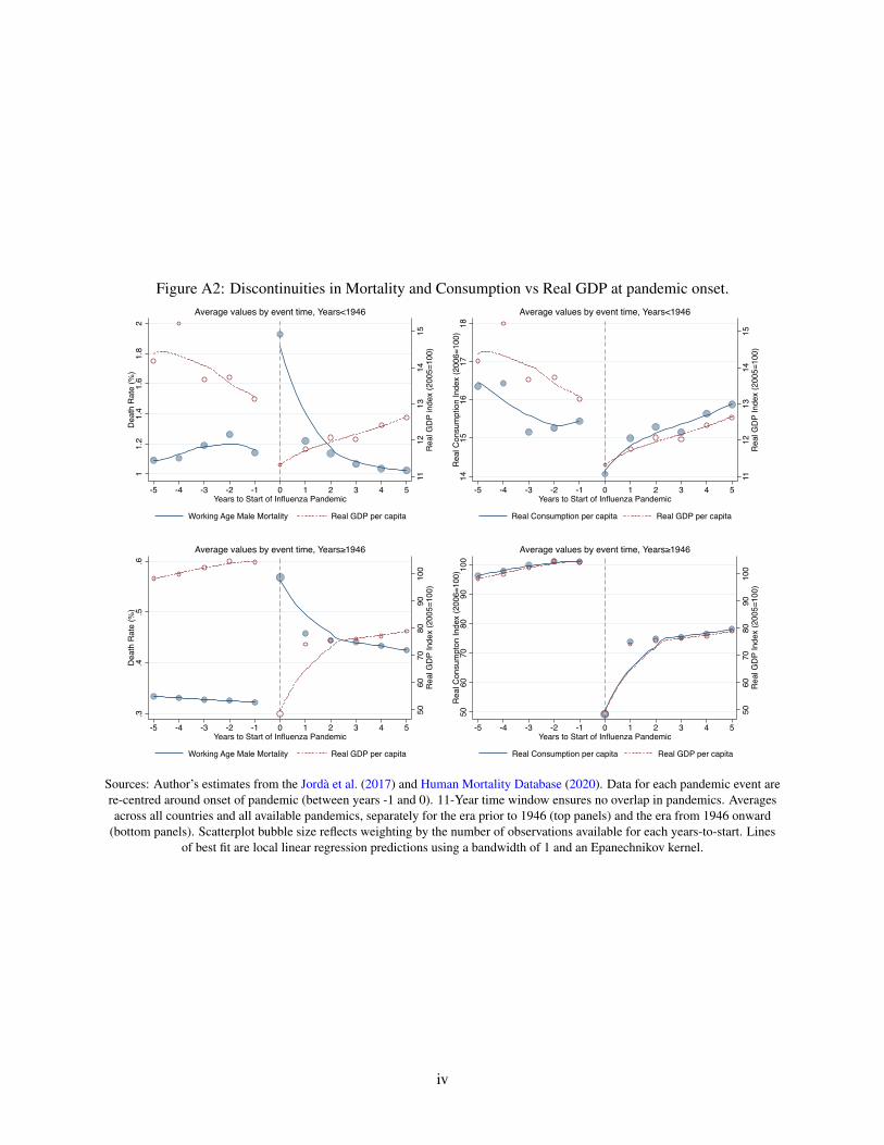
Figure A2: Discontinuities in Mortality and Consumption vs Real GDP at pandemic onset.

1112

1314

15R

eal G

DP

inde

x (2

005=

100)

11.

21.

41.

61.

82

Dea

th R

ate

(%)

-5 -4 -3 -2 -1 0 1 2 3 4 5Years to Start of Influenza Pandemic

Working Age Male Mortality Real GDP per capita

Average values by event time, Years<1946

1112

1314

15R

eal G

DP

Inde

x (2

005=

100)

1415

1617

18R

eal C

onsu

mpt

ion

Inde

x (2

006=

100)

-5 -4 -3 -2 -1 0 1 2 3 4 5Years to Start of Influenza Pandemic

Real Consumption per capita Real GDP per capita

Average values by event time, Years<1946

5060

7080

9010

0R

eal G

DP

Inde

x (2

005=

100)

.3.4

.5.6

Dea

th R

ate

(%)

-5 -4 -3 -2 -1 0 1 2 3 4 5Years to Start of Influenza Pandemic

Working Age Male Mortality Real GDP per capita

Average values by event time, Years≥1946

5060

7080

9010

0R

eal G

DP

Inde

x (2

005=

100)

5060

7080

9010

0R

eal C

onsu

mpt

on In

dex

(200

6=10

0)

-5 -4 -3 -2 -1 0 1 2 3 4 5Years to Start of Influenza Pandemic

Real Consumption per capita Real GDP per capita

Average values by event time, Years≥1946

Sources: Author’s estimates from the Jorda et al. (2017) and Human Mortality Database (2020). Data for each pandemic event arere-centred around onset of pandemic (between years -1 and 0). 11-Year time window ensures no overlap in pandemics. Averagesacross all countries and all available pandemics, separately for the era prior to 1946 (top panels) and the era from 1946 onward

(bottom panels). Scatterplot bubble size reflects weighting by the number of observations available for each years-to-start. Linesof best fit are local linear regression predictions using a bandwidth of 1 and an Epanechnikov kernel.

iv