WORKING PAPERS IN ECONOMICS

No 301

Executive Compensation and Macroeconomic

Fluctuations

Lars Oxelheim, Clas Wihlborg, and Jianhua Zhang

April, 2008

ISSN 1403-2473 (print) ISSN 1403-2465 (online)

SCHOOL OF BUSINESS, ECONOMICS AND LAW, UNIVERSITY OF GOTHENBURG Department of Economics Visiting adress Vasagatan 1, Postal adress P.O.Box 640, SE 405 30 Göteborg, Sweden Phone + 46 (0)31 786 0000

Executive Compensation and Macroeconomic Fluctuations

Lars Oxelheim

Lund University and Research Institute of Industrial Economics

Clas Wihlborg Chapman University and Copenhagen Business School

Jianhua Zhang

University of Göteborg

April 18, 2008

Forthcoming in Oxelheim, L. and C. Wihlborg (2008), Markets and Compensation for Executives in Europe, Emerald Publishing, Oxford.

Abstract Macroeconomic fluctuations affect corporations’ performance through demand and cost conditions. Incentive effects of performance-based compensation schemes for management may be weakened or biased by macroeconomic influences if management is unable to forecast macroeconomic fluctuations or unable to adjust operations in response to changes in macroeconomic conditions. In this paper we analyze the impact of macroeconomic, industry and firm-specific factors on salaries and bonus of CEOs in 131 Swedish corporations during the period 2001-2006. A distinction is made between anticipated and unanticipated macroeconomic fluctuations. The macroeconomic influences on performance and compensation can be expected to vary from firm to firm in terms of magnitude of effects, as well as in terms of relevant macroeconomic variables. The estimates obtained in this paper refer to the average impact across the sample of firms. We find that the average Swedish CEOs’ compensation is explained to a substantial extent by macroeconomic factors; less so by unanticipated factors alone. Key words: executive compensation, macroeconomic factors, cash compensation JEL: L14, L16, M14, M21, M52

1

1. Introduction

Executive compensation is under scrutiny on both sides of the Atlantic. Although the

level of compensation in Europe is below that in the US, European compensation levels

have been catching up and increased rapidly during the last five years. It is not only the

level of compensation that causes debate but also the timing of large payments to

executives relative to earnings of firms, and relative to increases in labor costs and real

income in a country. There are times when the public perceives large payments to

executives as particularly controversial. One possible source of such perceptions is

developments in the macro economy. If, for example, performance linked compensation

increases substantially as a result of domestic or international macroeconomic

developments, these increases may be considered a windfall for management. If this

happens during a period when unemployment is high and wage increases low, a high

compensation level may be considered particularly undeserved. In other scenarios, the

contribution of the macro economy to changes in compensation could be negative. One

objective of this paper is to estimate what share of changes in executive compensation is

explained by macroeconomic developments during the period 2001-2006.

The economic motivation for analyzing the impact of macroeconomic

fluctuations on executive compensation is that changes in performance-based

compensation caused by macroeconomic events may weaken or distort incentives of

management to focus their efforts on enhancing the firm’s competitiveness and

shareholder value. A large share of changes in compensation will be based on factors

entirely beyond executives’ control, if macroeconomic drivers of performance cannot be

forecast, or if production and sales efforts cannot be adjusted to take advantage of

macroeconomic developments.

Macroeconomic fluctuations can be expected to have a substantial impact on the

performance of most firms and, thereby, on performance-linked compensation. The

impact on the performance of any particular firm depends on the macroeconomic

sensitivity of each firm’s particular business, and on what aspect of performance we are

concerned about. Cash flows and earnings can be expected to be more sensitive to

macroeconomic shocks than sales for most firms, since costs are netted out to obtain the

former performance measures. The macroeconomic impact on stock market returns

should be smaller than the impact on cash flows and earnings, since stock returns reflect

2

expectations for relatively long periods over which macroeconomic fluctuations tend to

cancel out. Thus, the effects of macroeconomic fluctuations on the time pattern of

executive compensation payments will depend on the link between compensation and

the different aspects of performance, as well as on the sensitivity of relevant

performance measures to macroeconomic events.

In Oxelheim and Wihlborg (2003) the case of Electrolux was used to illustrate

how changes in performance can be decomposed into one “intrinsic” component and

one component caused by macroeconomic developments. They used a set of domestic

and foreign macroeconomic price variables (exchange rates, interest rates, price levels)

to filter out the macroeconomic component from total changes in performance from

quarter to quarter. The reason for using price variables is that they can be observed

without a long lag. Therefore, they can be used to decompose very recent changes in

performance and, thereby, to adjust compensation. The particular price variables

employed in the decomposition could vary from firm to firm depending on product and

market characteristics.

In this paper we decompose changes in compensation rather than in a

performance measure in order to analyze what share of compensation-changes were

caused by anticipated and unanticipated macroeconomic developments for the average

Swedish publicly traded firms during the period 2001-2006. Presumably, changes in

compensation net of these factors represent compensation for changes in firms’

“intrinsic” competitiveness. We control for industry factors as well. One set of

macroeconomic variables are used in the decomposition for all firms. Thereby, the

macroeconomic influences on performance in many firms could be underestimated,

since the appropriate set of variables is likely to be firm-specific.

Macroeconomic effects on compensation can occur through a number of

channels depending on what aspects of performance affect salaries and bonus of CEOs.

We distinguish between effects on salaries and on bonus and we analyze the extent to

which the macroeconomic effects depend on their impact on common performance

measures like sales and market values versus influences on salaries and bonus through

aspects of performance that we cannot identify. Boards in some firms may have stable

salaries and predetermined rules for bonus payments based on a particular performance

measure. Other boards may set the CEO salary based on a number of criteria that can

3

vary from period to period but, nevertheless, create a systematic relation between

macroeconomic factors and compensation.

Some early studies of executive compensation across firms focused on the

relation between CEO compensation and firm performance (Coughlan and Schmidt,

1985; Murphy, 1985, 1986; Jensen and Murphy, 1990; Abowd, 1990; Leonard, 1990),

while other studies analyzed whether CEOs are rewarded for performance relative to the

market or relative to industry factors (Antle and Smith, 1986; Gibbons and Murphy,

1990; Bebchuk and Grinstein 2005). Whether CEO compensation is more closely tied to

firm size or firm profits is controversial due to a multicolinearity problem among the

independent variables in the regressions (Ciscel and Carroll, 1980; Rosen, 1992).

We focus on the impact of macroeconomic and industry factors, as well as firm-

specific factors, on salaries and bonus of CEOs in Swedish firms during the period

2001-2006. After estimating the impact of macroeconomic factors along with firm and

industry factors for the period 2001-2005, we ask how salaries and bonus would have

developed for the average firm during the estimation period had they been independent

of total and unanticipated macroeconomic fluctuations. Using the same coefficients we

also calculate the impact of macroeconomic factors on compensation in 2006 for a

smaller set of firms.

In Section 2, we discuss in more detail how managerial incentives are influenced

by macroeconomic influences on compensation. The data set for compensation in the

form of salary and bonus is described in Section 3. Firm-specific and industry factors

explaining compensation are analyzed in Section 4. The contribution of macroeconomic

factors to compensation and performance measures is estimated in Section 5 using

cross-section and panel analyses. In Section 6 we decompose compensation each year

into an “intrinsic” component and a component caused by macroeconomic factors

distinguishing between the total impact of the macro economy and the unanticipated

impact. In section 7 we test whether there is simultaneity between performance and

compensation, and we ask whether the results hold across industries and size groups.

Concluding comments follow in Section 8.

4

2. Macroeconomic Fluctuations and Managerial Incentives

Macroeconomic factors, as well as industry wide factors, are beyond managerial

influence and control. To the extent these factors cannot be forecast, while influencing

performance linked compensation, macroeconomic fluctuations create noise in the

relation between compensation and the performance that can actually be influenced by

management. Such noise weakens the incentive-effects of performance-based

compensation schemes if managers are risk-averse (see e.g. Milgrom and Roberts,

1992).

Management is able to reduce the impact of macroeconomic fluctuations on

performance measures and, thereby, on compensation by means of risk management

techniques and investments in flexibility (real options). A risk averse manager, whose

compensation depends on macroeconomic fluctuations, has the incentive to employ risk

management techniques excessively, if shareholder value does not increase with

reduced performance-variance (Smith and Stulz, 1985). Thus, to the extent

compensation can be made independent of unanticipated macroeconomic fluctuations,

managers’ incentives with respect to risk management would be more closely aligned

with shareholders’ objectives.

Management may have some control over the impact of anticipated

macroeconomic fluctuations on performance. For example, production capacity can be

raised in response to a forecast of an increase in aggregate demand in the economy, or

shifted towards countries with cost advantages in response to a forecast of changes in

real exchange rates. Such changes in the production capacity and in other aspects of

operations are likely to require some lead time. In some firms the lead time may exceed

the time horizon for which macroeconomic developments can be forecast.

The ability to adjust capacity and operations in response to changes in

expectations about macroeconomic conditions varies across firms. If there is little

adjustability within the time horizon for macroeconomic forecasting, then management

cannot influence performance effectively in response to expected macroeconomic

developments. Accordingly, if compensation were based on performance that depends

on macroeconomic developments, managers could form expectations about increases or

decreases in compensation based on expected macroeconomic developments. These

expectations could bias managers’ incentives to exert effort effectively. Specifically, an

5

expected decrease in compensation could induce managers to try to compensate in the

short term by measures that enhance short-term performance but not necessarily

shareholder value. For example, they may be induced to speculate on changes in interest

rates and exchange rates. An expected increase in compensation could induce

management to relax their efforts to enhance performance in other ways, as well as

induce them to speculate in financial markets. If compensation instead were based on

performance net of macroeconomic influences, managers’ incentives would be to exert

effort in areas where they would be able to increase shareholder value.

There exist firms where capacity and operations can be adjusted relatively fast

and effectively in response to expectations about macroeconomic developments. In this

case, managers should have the incentive to make these adjustments. Compensation

based on performance including expected macroeconomic influences, but excluding

unanticipated macroeconomic influences, would provide appropriate incentives in these

firms.

Compensation based on total performance including all macroeconomic

influences would provide appropriate incentives for management only if value-

enhancing adjustment of capacity and operations can be made immediately in response

to changes in the macroeconomic environment. Such firms are most likely rare with

possible exceptions in the service sector.

Investments in flexibility (real options) increase shareholder value in many firms

and they reduce the impact of relatively large changes in macroeconomic factors on

performance measures. In other words, flexibility tends to introduce a non-linear

relation between performance and risk-factors. Compensation schemes should be

designed in such a way that they provide incentives to invest in flexibility to respond to

macroeconomic events. Oxelheim and Wihlborg (2003) argue that if compensation is

adjusted for macroeconomic fluctuations based on a fixed linear relation between these

fluctuations and performance, then the incentives to invest in flexibility (real options)

are retained.

3. The Compensation Data

Our dataset covers compensation for CEOs as well as Board Chairmen. Data have been

collected from annual reports for all Swedish firms listed on the stock exchange as

6

Large-Cap, Mid-Cap, and Small-Cap 1 firms during the period 2001-2006. Only

compensation in the form of cash disbursements, i.e. salaries and bonus, are included,

while stock option awards are not included. Since the compensation to Board chairmen

do not show much variation over time and many data-points are missing, we limit the

analysis to CEOs.

The firm’s specific factors are collected from DataStream, while the

macroeconomic factors are obtained from EcoWin (Reuters) database.

Table 1 reports mean and median compensation levels in million SEK for the

CEOs in Swedish firms from the different lists on the Stockholm Stock Exchange

during the period 2001-2006. There are 131 firms during the period 2001-2005, but only

83 firms for 2006. Therefore, the estimations below will be carried out using the sample

2001-2005. The 2006 data will be used for “out of sample” prediction of

macroeconomic influences based on estimates for the earlier years.

The index for average CEO compensation for each year is displayed both in

Table 1 (Index=100 in 2001) and in Figure 1. We can see that the compensation levels

increased during the period 2001-2005 in all the firms as well as in different sub-groups

of firms. On average, the compensation increased 42 percent. In the Large-cap firms it

increased 36 percent. The largest increase, 63 percent, occurred in the Mid-cap firms

while the increase in the Small-cap firms was 40 percent. Based on our smaller sample

for 2006, the increase in compensation continued to an average index of 158 in this year.

For Large-cap, Mid-cap and Small-cap firms the 2006 index figures reached 140, 169

and 141, respectively.

(Insert Table 1 and Figure 1 Here)

In Table 2 a distinction is made between salary and bonus for the years 2002-

2006. The firms included in Table 2 are the same as in Table 1. The year 2001 is

excluded here because we could not separate the bonus from the salary for this year.

Some firms did not pay bonus at all during the period while others may have paid bonus

only in some years. It would seem to be reasonable to assume that when a firm starts to

pay bonus it continues. A few firms stopped paying bonus during this period. In all 21 1 It is grouped according to the market capitalization of the firm. Large-Cap > 1 billion Euro; 150 mil Euro < Mid-Cap < 1 billion Euro; Small-Cap < 150 million Euro.

7

out of the 131 firms stopped bonus payments during the period but many more began

paying bonus. In 2001, 68 firms did not pay bonus while in 2005 this figure had shrunk

to 33. Table 2 shows that bonus payments increased much faster than salary payments.

Bonus payments increased 165 percent, while salaries increased only 14 percent. The

former figure takes into account both that average bonus payments increased and that

the number of firms paying bonus increased.

(Insert Table 2 Here)

4. Explaining Compensation without Macroeconomic Factors

In order to first identify the most important firm-specific factors explaining CEO-

compensation, the above compensation sample is matched with firm performance

variables. After eliminating the missing values in the firm performance sample, our final

sample contains different numbers of firms in different years. Thus, the panel is

unbalanced with a maximum of 126 firms and a minimum of 122 firms in the period

2001-2005. The 2006 sample is not used in panel regressions since it contains only 83

firms.

We begin by analyzing how the cross-section variation of compensation levels

(salary plus bonus) for the CEOs depends on a number of firm-and industry specific

performance measures, and we ask whether the cross section pattern is stable over the

data period. The following regression is estimated in cross-section for each year, as well

as pooled:

tiii

i

tititi

dummiesIndustry

ePerformancLogSalesLogonCompensatiLog

,

8

3

,2,10, )()()(

εα

ααα

++

++=

∑=

(1)

In order to minimize the multicolinearity problem, we focus on variables and

ratios that exhibit relatively little correlation with each other. The firm’s total sale is

used as a proxy for firm size. A number of performance variables were tested in

equation (1) to find which one(s) explains compensation the best. The variables were

return on assets, return on equity, and Tobin’s Q. We found that Tobin’s Q (measured as

8

market value relative to book value) had the most explanatory power and the least

correlation with non-performance variables. Therefore, Tobin’s Q is used as the

performance proxy from now on. Seven industry dummies are used to control for the

industry factors.2

All the variables in the regressions in this study are in logarithms. Therefore, the

regression coefficients are interpreted as “compensation-performance elasticities” rather

than “compensation-performance sensitivities”. One of the advantages of the elasticity

approach is that it produces a better “fit” in terms of marginal effects. Another

advantage is that the elasticity is relatively invariant to firm size while sensitivities vary

monotonically with firm size (larger firms having smaller betas) (Gibbons and Murphy,

1992; Murphy 1998).

Table 3 shows the results for equation (1) for each year and for pooled data. It

can be seen that the elasticity with respect to sales remains fairly constant from year to

year while the elasticity with respect to Tobin’s Q seems to have increased year by year

from 2002. The elasticity coefficients for 2006 based on a smaller sample are very close

to the coefficients in the pooled regression for 2001-2005. Nevertheless, we exclude

2006 in the regressions below.

The only industries showing a significant difference from the average are

industry 4 (health care) and, to a lesser extent, industry 3 (financials). Compensation

levels in these industries have increased relatively fast.

(Insert Table 3 Here)

Using the above firm specific factors, we estimate two random effects models

with industry dummy variables in one and time dummy variables in the other. The

results are reported in Table 4. The results for the random effects Model 1 with industry

factors is very similar to the results for pooled data in Table 3 except that the dummy

for industry 3 is not significant. Thus, competitive conditions in particular industries do

not seem to influence compensation much.

2 The industries are: 1) consumer goods, 2) energy, 3) financials, 4) health care, 5) industrials, 6) information technology and telecommunication services, and 7) materials.

9

The time dummy variables are highly significant in the second column of Table

4. The coefficients increase each year from 2001-2005. The time pattern could be

caused by macroeconomic influences. We return to this issue below.

(Insert Table 4 Here)

Are the patterns for salary and bonus different? It can be expected that the bonus

component of compensation is more sensitive than the salary component to

performance-variation over time and across firms. Therefore the model with industry

dummies is also tested for Salary and Bonus separately. The results are shown in Table

5. There are fewer observations for Salary and Bonus separately than for the sum of

these components, because all observations of zero Bonus are excluded. The Salary

component is explained mainly by sales, while Tobin’s Q has a strong effect on Bonus

but no effect on Salary. Clearly and not surprisingly, compensation in the form of bonus

is much more sensitive to performance from a shareholder perspective than salary

compensation. The table also shows that the results for Salary plus Bonus are similar to

the results for Bonus alone, although the coefficients for the total are generally smaller.

Since the results are so similar, and since we have twice as many observations for total

compensation as for Bonus alone, we focus on total compensation in the following

analysis of macro-factors.

(Insert Table 5 Here)

5. CEO-Compensation and Macroeconomic Factors

In this section we turn to an analysis of the macroeconomic influences on CEO-

compensation. These influences can occur through the performance variables in

equation (1) or through other variables influencing compensation. We investigate

whether macroeconomic variables affect compensation independently of variation in Q

and Sales, and we analyze macroeconomic influences on Q and Sales. The total

macroeconomic influence on compensation is the sum of these effects.

Macroeconomic conditions can be described using either quantity variables like

GDP, GDP growth, investments and employment, or using price variables like interest

10

rates, inflation and exchange rates. Although the former group of variables describes

macroeconomic conditions, they are typically observed with a substantial lag. Price

variables, on the other hand, can be seen as easily observable signals of underlying

macroeconomic shocks and developments. A shock would have a certain effect on a

group of price variables as well as on GDP, employment, etc. but only the former would

be observable at the time a shock occurs. Therefore, these signals can be useful tools for

decomposing compensation and performance into “intrinsic factors” and

macroeconomic factors. Another advantage of using price variables like interest rates

and exchange rates in the decomposition is that they adjust rapidly to both domestic and

foreign conditions affecting a firm’s performance. For these reason we prefer to use

only price variables as proxies for macroeconomic conditions in the following. 3

Specifically, we use exchange rates, interest rates, inflation and the market return in the

stock market.

It is likely that each firm’s performance is sensitive to its specific set of variables

but here we employ one set to explain changes in compensation across firms and time.

Thus, we obtain estimates for the macroeconomic impact on compensation for the

average firm. Dummy variables for firm characteristics could be introduced in the

analysis but we restrict the use of dummies to distinguish between industries as above,

and to separate relatively export dependent firms from others.

The following random effects model is specified to determine macroeconomic

influences on compensation independently of variation in Q-values and sales:4

3 An alternative formulation including GDP as well as price variables were tested as mentioned below. 4 The random effects model is estimated directly because of the inclusion of industry dummy variables, which are invariant across time for each firm.

11

tiiii

i

ti

titi

ti

ti

ti

ti

tititi

udummiesIndustry

rateinterestdAnticipateLogdummyExportdummyExportCPItedUnanticipaLogCPIdAnticipateLog

rateexchangedUnticipateLograteexchangedAnticipateLog

rateinterestdUnticipateLograteinterestdAnticipateLog

QsTobinLogSalesLogonCompensatiLog

,

16

11

,109

,8,7

,6

,5

,4

,3

,2,10,

)1()1()1(

)1()1(

)1()1(

)'()()(

εα

αααα

αααα

ααα

+++

+×++

Δ++Δ++

Δ++

Δ++

++

++

++=

∑=

(2a)

The assumptions about expectation formation are described below. Given those

assumptions the unanticipated exchange rate and the anticipated inflation dropped from

the model due to multicolinearity. Model 1 in Table 7 shows the results without these

variables. The unanticipated interest rate turned out to be insignificant. The correlations

in Table 6 reveal that the correlation between the anticipated and the unanticipated

exchange rate change is -0.95. Thus, we cannot identify whether anticipated or

unanticipated exchange rate effects are the most important. For this reason we include

the total exchange rate change in the following equation:

tiiii

i

ti

titi

tititi

udummiesIndustry

dummyExportCPItedUnanticipaLograteexchangeLograteinterestdAnticipateLog

QsTobinLogSalesLogonCompensatiLog

,

12

7

6,5

,4,3

,2,10,

)1()1()1(

)'()()(

εα

αααα

ααα

+++

+Δ++

Δ++++

++=

∑=

(2b)

The results of the estimation of equation (2b) are presented as Model 5 in Table

7. Before arriving at the formulations in equations (2a) and (2b) the market return in the

stock market was included as another macro price variable that could serve as a signal

of macroeconomic conditions. Neither the anticipated nor the unanticipated component

of this variable was significant, however. Furthermore, an alternative specification of

macroeconomic factors including GDP, the market return and the exchange rate change

12

was tested. The explanatory value of this formulation including GDP was much lower

than the present formulation. This result supports the idea that price variables serve as

useful signals of macroeconomic conditions.

The construction of anticipated and unanticipated changes in price variables can

be described using the following time line. The average yearly observations of interest

rates, exchange rates, and consumer prices are observed in each period. On the time line

period t is 2002.

The following assumptions are made with respect to the formation of

expectations: The expected interest rate in the next period is equal to the current interest

rate. Thus,

1−= tt irateinterestdAnticipate

1−−= ttt iirateinteresttedUnanticipa

The return on the 1-year Government bond is used as the interest rate.

The expected exchange rate change over the next year is reflected in the current

one-year interest rate differential (uncovered interest rate parity). Thus,

11 −− −=Δ tUSD

tSEK

t iirateexchangedAnticipate

[ ] [ ]111)/()/( −−− −−−=Δ tUSD

tSEK

ttt iiUSDSEKUSDSEKrateexchangetedUnanticipa

The exchange rate is SEK/US Dollars. All the changes are in percent.

The expected inflation over the next year is equal to the inflation last year. Thus,

21 −− −=Δ ttt cpicpiinflationdAnticipate

[ ] [ ]211 −−− −−−=Δ ttttt cpicpicpicpiinflationtedUnanticipa

The correlations between variables we have in cross-section and all other

variables are reported in Table 6. Among the price variables for which we have only

five observations, the market return is highly correlated with several other price

Year 2001 t-1

Year 2002 t

Year 2003 t+1

Year 2000 t-2

13

variables. This correlation explains why the market return is not significant in the

regressions.

(Insert Table 6 Here)

Table 7 shows the results when equation (2) is tested using the random effects

model.5 When macroeconomic variables are included in the random effects model with

firm specific and industry factors, the time dummies must be dropped. There are some

differences among the five models presented. In Model 1, both anticipated and

unanticipated interest rates are included. As noted, the latter is insignificant and dropped

to arrive at Model 2 in the table. In Model 3, a dummy for relatively export oriented

firms has been added on its own and interactively with the exchange rate. The

interactive term is insignificant and dropped in Model 4. Finally in Model 5, the full

exchange rate change is substituted for the anticipated exchange rate change, since the

correlation between the variables is almost perfect (and negative).

(Insert Table 7 Here)

The results in Table 7 show that CEO salaries and bonuses are positively and

significantly related to firm size and firm performance after controlling for

macroeconomic influences. The coefficients for both Sales and the Q-values are smaller

when macroeconomic influences are included explicitly in Table 7 in comparison with

Tables 3 and 4. Thus, it seems that macroeconomic influences occur through Sales and

Q, as well as through other channels. These other channels could be earnings or other

firm-specific performance measures. The particular variables used by corporate boards

to determine CEO compensation may even change from year to year. The fact that Sales

and Q are the performance variables with the greatest explanatory value indicates that

5 The robustness of the random effects model, Model 5, is further tested by using two alternative specifications, i.e. pooled, and fixed effects. Based on Breusch and Pagan Lagrangian Multiplier test and Hausman test, the pooled and fixed effects models can be rejected, yet the random effects model cannot be rejected. In addition, in order to detect multicolinearity among all the factors, the variance inflation factors (VIF) are estimated by using the pooled regression. The average VIF is 2.38, and the individual VIF is within the range 1.26-4.44. Therefore, multicolinearity does not seem a problem in the model.

14

much of the variation in compensation is linked to a time-varying set of performance

indicators.

CEO compensation changes by about 2.4% for each 10% change in firm size,

and it changes about 0.8% for each 10% change in firm performance as measured by Q.

The former finding is consistent with some findings from the US markets. Bebchuk and

Grinstein (2005) find in a US sample for the period 1993-2003 that a 10% change in the

firm size results in a 2.14% change in CEO compensation. They also find that a 10%

change in performance leads to a 2.11% change in compensation. Our results before

controlling for macroeconomic factors in Table 3 are consistent with these figures, but

when we control for macroeconomic factors the compensation effect of a change in

performance in Table 7 is less than a third of the effect in Table 3. In Section 7 below

we ask whether this result is robust when we allow for simultaneity between

performance and compensation.

Turning to the results for macroeconomic factors in Table 7, the anticipated

interest rate is negatively related to compensation. CEO compensation increases by

about 12% for each 1% point decline in the interest rate (approximately equal to 1% of

1+Anti. interest rate).

The results for exchange rate effects are harder to interpret as a result of the high

negative correlation between the proxies for anticipated and unanticipated exchange rate

changes. The proxy for anticipated exchange rate changes is positively correlated with

changes in compensation meaning that a depreciation of the SEK relative to the USD

raises compensation, while the proxy for unanticipated changes indicates the opposite.

As noted, the anticipated changes are almost perfectly correlated with unanticipated

changes and, therefore, with total exchange rate changes. We can simply not identify

whether effects of exchange rates are due to anticipated or unanticipated changes

although the variation in floating exchange rates tends to be dominated by unanticipated

changes. In Model 5, where the total exchange rate change is included, a depreciation of

the SEK has a negative effect on compensation. This sign is hard to explain for export-

oriented industries. It makes more sense for multinational firms with large parts of their

production abroad.

15

The export dummy interacting with the exchange rate change is insignificant in

Model 5. Exporting firms seems to have had a faster growth of compensation, however,

as shown by the significant export intercept dummy.6

We turn now to the impact of macroeconomic factors on the performance

measures, Sales and Q that systematically affect compensation. The following equation

is estimated for the Q-value:

tiiii

i

ti

titi

titi

udummiesIndustry

dummyExportCPIUnantiLograteexchangeLograteinterestAntiLog

SalesLogQsTobinLog

,

11

6

5,4

,3,2

,10,

).1()1().1(

)()'(

εα

αααα

αα

+++

+Δ++

Δ++++

+=

∑=

(3)

The Q-value is made a function of Sales, the macroeconomic variables identified above,

and dummy variables in equation (3). The regression for Sales includes the Q-value, as

well as the same macroeconomic and dummy variables.

Table 8 shows that Sales has a small negative impact on Q when controlling for

macroeconomic factors. This result indicates that sales generally are higher than what

value maximization would call for. The anticipated interest rate has a strong negative

effect on both variables. The exchange rate change affects Sales but not Q-values. A

depreciation increases Sales as can be expected. The export dummy variable is also

positive and significant indicating that the sales from export oriented firms are larger

than sales from other firms. Unanticipated inflation is positively related to Q, but there

is no significant relation with Sales.

(Insert Table 8 Here)

In the next section the estimates of macroeconomic influences on Sales, Q-

values, and on compensation at constant levels of Sales and Q will be used to

6 The compensation for the CEOs in the export firms is about 30% (which is (e0.206-1)*100) higher than in the non-export firms.

16

decompose compensation into one component explained by “intrinsic factors” and one

component explained by macroeconomic factors.

6. Filtering out Macroeconomic Influences on Compensation

How would compensation have developed if the impact on compensation of macro-

factors would have been filtered out? Table 9a shows the impact on compensation of the

total change in the macro variables for the period 2001-2005, while Table 9b displays

the impact of unanticipated changes in macro variables. In Table 10 the coefficients

above are used out of sample to analyze the impact of macro variables on compensation

in a smaller sample of firms for 2006.

In each of the tables 9a-10 column (1) shows the percent of salary plus bonus

caused by macroeconomic variables each year at constant levels of Q and Sales.

Columns (2) and (3) show the percent of Q and sales explained by the same variables.

Column (4) presents the sum of the effects in columns (1)-(3) using the coefficients in

Table 7 Model 5 as weights. Thus, column (4) shows the percent of salary plus bonus

explained by macroeconomic factors each year. In columns (5) and (6) we show the

macroeconomic effects as percent of bonus payments only. The macroeconomic effects

included in Tables 9b and 10b are caused by unanticipated changes alone.

Macroeconomic effects are calculated based on deviations from mean levels of

the macro variables during the period times the coefficients in Table 7, Model 5. The

procedure for calculating macroeconomic effects on Q and Sales is the same, but the

coefficients are obtained from Table 8. The mean levels of unanticipated changes are

zero.

Column (4) in Table 9a reveals that the macroeconomic factors through all three

channels had a large negative effect on compensation in 2001 (-16.6%). Thereafter the

macroeconomic factors had an increasingly positive effect on compensation each year

through 2005. In 2005 macroeconomic factors explained 21% of the compensation.

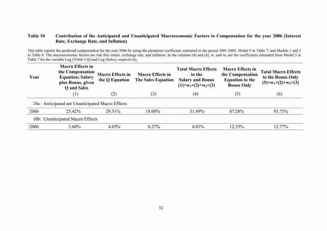
Table 10a shows that the trend continued in 2006. The average share of compensation

explained by macroeconomic factors is only around two percent. This small average

effect is the result of our assumption that macroeconomic effects occur when the

variables deviate from their mean values.

The total macro effects in column (4) are dominated by the independent effects

17

in column (1) although the macro effects on both Q and Sales are substantial.

The total macroeconomic effects each year as percent of bonus payments only

are presented in columns (6). Since bonus is only a part of total compensation the

macroeconomic effects here are larger. Table 10a shows that in 2006 macroeconomic

factors contributed to compensation an amount nearly equal (93.75%) the bonus

payments.

(Insert Table 9a, 9b and 10 Here)

The contribution of unanticipated macroeconomic effects are shown in Table 9b

for the period 2002-2005 and in 10b for 2006 under the assumption that the regression

coefficients based on the period 2001-2005 are valid for 2006 as well. The unanticipated

changes in macro variables include effects of exchange rate changes and inflation, and it

is assumed that all exchange rate changes are unanticipated.

The contribution of unanticipated macroeconomic factors to compensation is

smaller than the total effects in the previous table. The time pattern is also very different.

Table 9a Column (4) shows that the largest positive impact of unanticipated macro

factors on compensation between 2001 and 2005 occurred in 2003 (9%). The lowest

effect occurred the year after (-3%). Clearly, it would make a large difference whether

compensation levels would be adjusted for total macroeconomic influences or only

unanticipated influences.

The unanticipated macroeconomic effects on compensation are quite large

relative to bonus payments some years as shown in column (6). In 2003 compensation

explained by unanticipated macroeconomic variables amounted to more than half of the

bonus payments (58.53%). In 2006 the figure declined to 13% as shown in table 10b.

The effect of macroeconomic variables on changes in compensation is

sometimes even larger than the figures mentioned so far. Considering that the total

macroeconomic effect goes from negative 17% in 2001 to positive 32% in 2006, the

macroeconomic variables explain 59% ((132-83)/83) of the increase in CEO

compensation during the period 2001-2006. The effects can be even larger for

individual firms, since the estimates presented here represent the average across the

sample of firms.

18

7. Robustness to Size, Industry and Simultaneity

Compensation schemes vary across firms and the relevant macroeconomic variables, as

well as their impacts, vary across firms. For example, international firms are likely to be

sensitive to macroeconomic conditions abroad. We do not have the data to conduct

firm-level studies here but we can distinguish between size groups and industries.

Beginning with firms belonging to different levels of capitalization we run the

regressions in Table 7 for Large-Cap firms separately. The results are very similar to the

results presented for all firms in Table 7 in terms of coefficients as well as significance.

Therefore we do not show the results for Large-Cap firms here.

Turning to industries, the dummy for industry four (health care) was significant

in most of the regressions so it would be of interest to investigate this industry further.

However, there are only 5 firms with 40 observations in this industry. There are even

fewer firms in Industry 3 for which the industry dummy was significant in several

regressions. Financial institutions in general are different from corporations so we

ignore this sector as well.

Finally, we take into account that performance could depend on compensation.

After all, performance related compensation schemes are implemented with the

objective of enhancing managerial effort on behalf of shareholders. If compensation

schemes are successful, we expect the intercept term representing a constant rate of

growth of compensation to be larger for firms with high sensitivity to performance. We

cannot observe firm differences in this respect, however. It is also possible that firms

with a stronger performance-compensation link will have relatively strong performance

during periods when compensation is high as a result of manager’s greater effort on

behalf of shareholders. If so, there is a potential simultaneity problem between Tobin’s

Q, in particular, and compensation in the above regressions.

Table 11 shows the results of regressions using a two stage procedure to explain

compensation in comparison with the results of Model 5 in Table 7. The results for this

model are also reproduced in Table 11. Instrumental variables, including sales and all

anticipated and unanticipated macro variables in our data set, were used to estimate

Tobin’s Q in the first stage. The results in Table 11 show that the coefficient for Tobin’s

Q becomes almost three times as large as in the previous regressions and significant.

19

Thus, it is possible that there is some mutual dependence between performance and

compensation. All other coefficients remain nearly unchanged, however.

(Insert Table 11 Here)

In order to further investigate the endogeneity of the Q, the Hausman Test,

which tests the random effects model (REM) against the random effects model with

instrumental variables (IVREM), is reported in Table 11. Based on the Hausman test,

the random effects model with instrumental variables in the last column of the table is

rejected. Thus, the exercise performed in the previous sections with respect to the role

of macroeconomic factors should not be seriously affected by simultaneity.

8. Conclusions

We have argued that managerial incentives to maximize shareholder value can become

distorted or weakened by macroeconomic influences on performance and compensation.

In particular, if macroeconomic conditions cannot be forecast for a period that allows

production capacity and other aspects of corporate operations to be adjusted, then

compensation should be made independent of macroeconomic influences. If substantial

adjustment is feasible in response to expectations about the macroeconomy,

compensation should be made independent of unanticipated macroeconomic influences.

Firms differ with respect to adjustability of structure, capacity and operations,

and they differ in terms of their sensitivity to macroeconomic fluctuations. Analysis of

the dependence of a particular firm’s performance and CEO-compensation on

macroeconomic conditions requires data for performance, compensation, and relevant

macroeconomic data for a substantial period. Lacking such data we are restricted to

analyze macroeconomic influences on CEO compensation in 131 Swedish firms for the

period 2001-2005 using the same set of macroeconomic factors for all firms. A smaller

sample of firms for 2006 is analyzed as well. Using pooled data we identify the average

impact of macroeconomic factors on Swedish firms. Industry level analysis is also

constrained by an insufficient number of firms within each industry.

Three channels of macroeconomic influences on compensation are identified.

Macroeconomic factors affect sales and Q-values, and they affect compensation through

20

other variables that affect compensation in a less systematic way than sales and Q. The

macroeconomic factors we identify as important for the aggregate performance and

compensation in the Swedish firms are the exchange rate, the interest rate and the

inflation rate. These macroeconomic price variables are viewed as signals of underlying

macroeconomic shocks. As such, they are easily observable and useful for decomposing

performance and compensation into an “intrinsic” component and a macroeconomic

component.

After estimation of the sensitivities of performance variables and compensation

to the macroeconomic factors we use the coefficients in combination with

macroeconomic developments each year to calculate how compensation would have

developed had macroeconomic influences been filtered out each of the years 2001

through 2006. The calculations show that compensation would have developed very

differently had compensation been made independent of macroeconomic fluctuations.

Macroeconomic factors explain a 60 percent increase in compensation during the period.

Looking at the effects of macroeconomic variables on compensation as percent

of bonus payments we observe even larger effects. In 2006 the macroeconomic

contribution to compensation was as large as the bonus payments.

Unanticipated factors explain a smaller part of compensation. In 2003 these

factors explained 9 percent of compensation, while in 2004 the same factors reduced

compensation by 3 percent. As percent of bonus payments the corresponding figures

were larger; 59 percent and -7 percent, respectively. These figures may underestimate

the impact of unanticipated macroeconomic developments on the average Swedish firm

since they are based on the assumption that the average impact over the period is zero.

References Abowd, J. (1990), “Does Performance-Based Managerial Compensation Affect Corporate Performance?” Industrial and Labor Relations Review, 43(3), 52-73. Antle, R. and A. Smith (1986), “An Empirical Investigation of the Relative Performance Evaluation of Corporate Executives”, Journal of Accounting Research, 24(1), 1-39. Bebchuk, L. and Y. Grinstein (2005), “The Growth of Executive Pay”, Oxford Review of Economic Policy, 21, 283-303.

21

Ciscel, D. and T. Carroll (1980), “The Determinants of Executive Salaries: An Econometric Survey”, Review of Economics and Statistics, 62(1), 7-13. Coughlan, A. and R. Schmidt (1985), “Executive Compensation, Management Turnover, and Firm Performance: An Empirical Investigation”, Journal of Accounting and Economics, 7(1-3), 43-66. Gibbons, R. and K. J. Murphy (1990), “Relative Performance Evaluation for Chief Executive Officers”, Industrial and Labor Relations Review, 43(3), 30-51. Leonard, J. (1990), “Executive Pay and Firm Performance”, Industrial and Labor Relations Review, 43(3), 13-29. Mehran, H. (1995), “Executive Compensation Structure, Ownership, and Firm Performance”, Journal of Financial Economics, 38(2), 163-84. Milgrom, P. and J. Roberts (1992), Economics of Organization and Management, Prentice Hall. Murphy, K. J. (1985), “Corporate Performance and Managerial Remuneration: An Empirical Analysis”, Journal of Accounting and Economics, 7(1-3), 11-42. Murphy, K. J. (1986), “Incentives, Learning, and Compensation: A Theoretical and Empirical Investigation of Managerial Labor Contracts”, Rand Journal of Economics, 17(1), 59-76. Murphy, K. J. (1999), “Executive Compensation”, in Handbook of Labor Economics, 3, edited by Ashenfelter, O. and D. Card, North-Holland, Amsterdam, 2485-2563. Oxelheim, L. and C. Wihlborg (2003), “Recognizing Macroeconomic Fluctuations in Value Based Management”, Journal of Applied Corporate Finance, 15(4), 104-110. Oxelheim, L. and C. Wihlborg (2005), Corporate Performance and Exposure to Macroeconomic Fluctuations, Norstedts Academic Publishers, Stockholm. Rosen, S. (1992), “Contracts and the Market for Executives”, in Contract Economics, edited by Werin, L. and H. Wijkander, Blackwell Publishers. Smith, W., and R. Stulz (1985), “The Determinants of Firms’ Hedging Policies”, Journal of Financial and Quantitative Analysis, 20(4), 391-405.

22

Table 1 Mean and Median Compensation Levels: Salary and Bonus 2001-2006 This table displays mean and median compensation levels (Million SEK) for the CEOs in Swedish firms during the period 2001-2005 plus 2006. Compensation in any given year is defined as the sum of salary and bonus.

Year 2001

Year 2002

Year 2003

Year 2004

Year 2005 Year

2006

Panel A: All-Cap (n=131) (n=83) Mean 3.954 4.027 4.418 4.934 5.596 6.259 Index 100 102 112 125 142 - Median 2.500 2.600 2.914 3.300 5.082 4.510 Standard Deviation 4.010 3.708 4.111 4.381 5.082 4.966 Panel B: Large-Cap (n=48) (n=35) Mean 7.250 7.377 8.010 8.807 9.896 10.164 Index 100 102 110 121 136 - Median 5.796 6.328 6.567 7.441 8.702 8.400 Standard Deviation 5.020 4.299 4.861 4.898 5.992 5.318 Panel C: Mid-Cap (n=37) (n=29) Mean 2.359 2.471 2.949 3.367 3.854 3.981 Index 100 105 125 143 163 - Median 2.340 2.427 2.914 3.262 3.648 3.794 Standard Deviation 0.934 1.010 1.327 2.076 2.059 1.873 Panel D: Small-Cap (n=46) (n=19) Mean 1.799 1.782 1.852 2.152 2.511 2.543 Index 100 99 103 120 140 - Median 1.618 1.789 1.886 2.160 2.256 2.469 Standard Deviation 1.005 0.698 0.682 0.999 1.332 0.949

23

Table 2 Mean and Median Compensation Levels: Salary and Bonus 2002-2006 This table displays mean and median compensation levels (Million SEK) for the CEOs in Swedish firms during the period 2002-2005 plus 2006. Compensation in any given year is defined as salary or bonus. The firms included in this sample are the same as in Table 1.

Year 2002

Year 2003

Year 2004

Year 2005 Year

2006

Panel A: Salary (n=131) (n=83) Mean 3.350 3.569 3.628 3.803 4.443 Index 100 107 108 114 - Median 2.400 2.528 2.561 2.745 3.442 Standard Deviation 2.808 3.098 2.755 2.921 3.054 Panel B: Bonus (n=131) (n=83) Mean 0.677 0.849 1.305 1.794 1.823 Index 100 126 193 265 - Median 0.001 0.150 0.436 0.700 0.852 Standard Deviation 1.507 1.678 2.172 2.868 2.769 Number of the Firms without Paying Bonus 68 57 41 33 23

24

Table 3 Pooled and Cross-Sectional Regressions 2001-2006 without Macro Variables This table reports the parameter estimations from both pooled and cross-sectional regressions from equation (1). The dependent variable is Log (Compensation). The industries are: 1) consumer goods, 2) energy, 3) financials, 4) health care, 5) industrials, 6) information technology and telecommunication services, and 7) materials. The dummy 7 is dropped in the model.

Year 2001-2005

Year 2001

Year 2002

Year 2003

Year 2004

Year 2005

Year 2006

Log (Sales) 0.277*** 0.291*** 0.268*** 0.238*** 0.292*** 0.302*** 0.264*** (26.22) (12.66) (12.02) (9.93) (11.98) (11.75) (8.34) Log (Tobin’s Q) 0.199*** 0.093 0.065 0.189* 0.266*** 0.294*** 0.161* (5.23) (1.14) (0.77) (1.81) (2.72) (3.15) (1.58) Industry Dummy 1 0.090 0.235 0.066 0.094 0.057 0.044 -0.038 (0.84) (0.98) (0.30) (0.36) (0.23) (0.17) (-0.14) Industry Dummy 2 0.183 0.236 0.111 0.123 0.069 0.372 0.493 (0.84) (0.57) (0.28) (0.27) (0.17) (0.85) (1.11) Industry Dummy 3 0.260*** 0.320 0.077 0.243 0.351 0.300 0.335 (2.64) (1.44) (0.38) (1.04) (1.63) (1.32) (1.27) Industry Dummy 4 0.576*** 0.759*** 0.561** 0.590* 0.464 0.612** 0.335 (4.49) (2.65) (2.13) (1.88) (1.62) (2.07) (0.94) Industry Dummy 5 0.120 0.277 0.089 0.096 0.103 0.043 0.170 (1.29) (1.32) (0.47) (0.43) (0.50) (0.20) (0.70) Industry Dummy 6 0.117 0.314 0.067 -0.001 0.103 0.111 0.220 (1.17) (1.39) (0.33) (-0.00) (0.46) (0.48) (0.84) Constant 10.703*** 10.257*** 10.880*** 11.319*** 10.488*** 10.385*** 11.071*** (56.76) (24.77) (27.67) (26.25) (24.18) (22.46) (19.12) Observations 626 122 126 126 126 126 83 Adjusted R2 56% 59% 58% 48% 56% 54% 48% 1. t-values are in round parentheses. 2. *, **, *** denotes significance at the 0.10, 0.05 and 0.01 level or better.

25

Table 4 Random Effects Model with either Industry or Time Dummy Variables This table reports the parameter estimations from two random effects models for the period 2001-2005. The dependent variable is Log (Compensation). In the first model the industry dummies are used, while in the second model the time dummies are used. The industries are: 1) consumer goods, 2) energy, 3) financials, 4) health care, 5) industrials, 6) information technology and telecommunication services, and 7) materials. The time dummies are the years 2001-2005. The industry dummy variable 7 is dropped in the first model, while the time dummy variable for the year 2001 is dropped in the second model.

Model 1 Model 2

Log (Sales) 0.263*** 0.235*** (15.02) (13.98) Log (Tobin’s Q) 0.166*** 0.057* (4.77) (1.54) Industry Dummy 1 0.111 - (0.55) Industry Dummy 2 0.153 - (0.43) Industry Dummy 3 0.252 - (1.35) Industry Dummy 4 0.569** - (2.42) Industry Dummy 5 0.132 - (0.75) Industry Dummy 6 0.101 - (0.54) Year Dummy 2002 - 0.076** (2.11) Year Dummy 2003 - 0.172*** (4.98) Year Dummy 2004 - 0.221*** (6.36) Year Dummy 2005 - 0.305*** (8.56) Constant 10.925*** 11.379*** (33.98) (45.01) Observations 626 626

Log likelihood-ratio test -277.54*** [0.000]

-243.56*** [0.000]

1. t-values are in round parentheses, and p-values are in square parentheses. 2. *, **, *** denotes significance at the 0.10, 0.05 and 0.01 level or better.

26

Table 5 Random Effects Model using Salary, Bonus or Salary plus Bonus as Dependent Variable This table reports the parameter estimations from three random effects models. The dependent variable is Log (Salary), Log (Bonus), or Log (Salary plus Bonus). The industries are: 1) consumer goods, 2) energy, 3) financials, 4) health care, 5) industrials, 6) information technology and telecommunication services, and 7) materials. The industry dummy variable 7 is dropped in the models. The time period is 2002-2005. The regressions are based on the sample that firm pays bonus for the year.

Log (Salary)

Log (Bonus)

Log (Salary plus Bonus)

Log (Sales) 0.260*** 0.385*** 0.293*** (16.73) (8.76) (15.89) Log (Tobin’s Q) -0.006 0.484*** 0.128*** (-0.16) (3.61) (2.94) Industry Dummy 1 0.203 0.213 0.209 (1.37) (0.51) (1.15) Industry Dummy 2 0.219 0.242 0.295 (0.83) (0.31) (0.92) Industry Dummy 3 0.270* 1.390*** 0.586*** (1.94) (3.59) (3.42) Industry Dummy 4 0.733*** 1.182** 0.870*** (3.77) (2.21) (3.62) Industry Dummy 5 0.022 0.345 0.137 (0.17) (0.96) (0.86) Industry Dummy 6 0.210 0.477 0.313* (1.50) (1.22) (1.83) Constant 10.874*** 7.006*** 10.498*** (39.71) (9.02) (32.12) Observations 310 310 310 Overall R2 71% 36% 67% 1. t-values are in round parentheses, and p-values are in square parentheses. 2. *, **, *** denotes significance at the 0.10, 0.05 and 0.01 level or better.

27

Table 6 Correlations for the Variables 2001-2005

Log

(Salary andBonus)

Log (Sales) Log (Q)

Log (1+Marke

return)

Log (1+Anti.

int. rate)

Log (1+Unati.int. rate)

Log (1+Anti. Δex. rate)

Log (1+Unanti.Δex. rate)

Log (1+Anti.ΔCPI)

Log (1+Unanti. ΔCPI)

Log (Salary and Bonus) 1 Log (Sales) 0.7162 1 Log (Tobin’s Q) 0.0262 -0.1973 1 Log (1+Market return) 0.0960 0.0012 -0.0022 1 Log (1+Anti. interest rate) -0.1541 -0.0404 -0.1751 -0.4951 1 Log (1+Unanti. interest rate) -0.0361 0.0169 -0.1498 0.0180 -0.0832 1 Log (1+Anti. Δexchange rate) 0.0733 -0.0149 0.0279 0.7996 -0.2569 -0.4271 1 Log (1+Unanti. Δexchange rate) -0.0260 0.0276 0.0447 -0.7244 -0.0392 0.3784 -0.9498 1 Log (1+Anti. ΔCPI) -0.0751 -0.0367 -0.1858 0.3001 0.4972 0.0574 0.5368 -0.7367 1 Log (1+Unanti. ΔCPI) -0.0798 -0.0005 -0.0316 -0.6661 0.4605 0.0997 -0.8416 0.7277 -0.4957 1

28

Table 7 Random Effects Model with Firm Specific Factors and Interest Rate, Exchange Rate and Inflation as Macroeconomic Factors This table reports the parameter estimations from five random effects models. The dependent variable is Log (Compensation). The industry dummy variables are: 1) consumer goods, 2) energy, 3) financials, 4) health care, 5) industrials, 6) information technology and telecommunication services, and 7) materials. The industry dummy variable 7 is dropped in the models. The time period is 2001-2005.

Model 1 Model 2 Model 3 Model 4 Model 5

Log (Sales) 0.245*** 0.246*** 0.235*** 0.235*** 0.236*** (13.74) (13.83) (12.90) (12.91) (12.93) Log (Tobin’s Q) 0.048 0.063* 0.062** 0.062* 0.076** (1.25) (1.78) (1.75) (1.76) (2.15) Log (1+Anti. interest rate) -12.163*** -11.947*** -12.092*** -12.092*** -15.009*** (-7.01) (-6.93) (-7.02) (-7.02) (-7.15) Log (1+Unanti. interest rate) -3.072 - - - - (-1.02) Log (1+Anti. Δexchange rate) 4.657*** 5.654*** 5.664*** 5.608*** - (2.57) (4.17) (3.68) (4.14) Log (1+Δexchange rate) - - - - -0.728*** (-3.82) Log (1+Unanti. ΔCPI) 4.657* 6.007** 5.997*** 5.996*** 5.149*** (1.69) (2.48) (2.48) (2.48) (2.16) Industry Dummy 1 0.185 0.176 0.282 0.282 0.273 (0.90) (0.86) (1.36) (1.36) (1.32) Industry Dummy 2 0.099 0.104 0.059 0.059 0.063 (0.27) (0.29) (0.17) (0.16) (0.18) Industry Dummy 3 0.222 0.224 0.339* 0.339* 0.340** (1.17) (1.19) (1.75) (1.75) (1.76) Industry Dummy 4 0.640** 0.628*** 0.673*** 0.673*** 0.660*** (2.67) (2.63) (2.85) (2.85) (2.80) Industry Dummy 5 0.155 0.151 0.165 0.165 0.161 (0.86) (0.85) (0.93) (0.93) (0.91) Industry Dummy 6 0.128 0.121 0.204 0.204 0.197 (0.68) (0.65) (1.08) (1.08) (1.04) Export Dummy - - 0.207** 0.206** 0.206** (2.17) (2.17) (2.17) Export Dummy× Log (1+Anti. Δexchange rate) - - -0.107 - - (-0.08) Constant 11.647*** 11.633*** 11.622*** 11.623*** 11.725*** (33.89) (33.94) (34.35) (34.38) (34.61) Observations 626 626 626 626 626 Log likelihood-ratio test -238.96***

[0.000] -239.48***

[0.000] -237.15***

[0.000] -237.15***

[0.000] -238.38***

[0.000] 1. t-values are in round parentheses, and p-values are in square parentheses. 2. *, **, *** denotes significance at the 0.10, 0.05 and 0.01 level or better.

29

Table 8 Random Effects Model with Tobin’s Q or Sales as Depended Variable and Interest Rate, Exchange Rate and Inflation as Macroeconomic Factors This table reports the parameter estimations from two random effects models. The industry dummy variables are: 1) consumer goods, 2) energy, 3) financials, 4) health care, 5) industrials, 6) information technology and telecommunication services, and 7) materials. The industry dummy variable 7 is dropped in the models. The time period is 2001-2005.

Q Equation Sales Equation

Log (Sales) -0.038*** - (-2.03) Log (Tobin’s Q) - -0.079 (-1.57) Log (1+Anti. interest rate) -17.531*** -11.454*** (-7.46) (-4.06) Log (1+Δexchange rate) -0.101 0.629*** (-0.45) (2.46) Log (1+Unanti. ΔCPI) 5.418*** -0.653 (1.95) (-0.20) Industry Dummy 1 0.639*** 0.627 (3.07) (0.749 Industry Dummy 2 -0.298 -2.029 (-0.82) (-1.37) Industry Dummy 3 -0.079 -0.487 (-0.40) (-0.61) Industry Dummy 4 0.939*** -2.532*** (3.99) (-2.689 Industry Dummy 5 0.241 -0.586 (1.36) (-0.81) Industry Dummy 6 0.526*** -1.823*** (2.76) (-2.38) Export Dummy 0.058 1.460*** (0.60) (3.88) Constant 1.384*** 15.119*** (3.98) (20.28) Observations 626 626 Log likelihood-ratio test -319.11***

[0.000] -565.56***

[0.000] 1. t-values are in round parentheses, and p-values are in square parentheses. 2. *, **, *** denotes significance at the 0.10, 0.05 and 0.01 level or better.

30

Table 9a Contribution of the Anticipated and Unanticipated Macroeconomic Factors to Compensation (Interest Rate, Exchange

Rate, and Inflation) This table reports the predicted anticipated and unanticipated macro effects in different years as well as the whole period 2001-2005 using Model 5 in Table 7, and the models in Table 8. The macroeconomic factors are risk free return, exchange rate, and inflation. In the column (4) and column (6), w1 and w2 are the coefficients for the variables Log (Tobin’s Q), and Log (Sales) in Table 7, Model 5. The average total macro effect to the bonus in the period 2002-2005 is 20.22%.

Year

Macro Effects in the Compensation Equation; Salary plus Bonus, given

Q and Sales

Macro Effects in the Q Equation

Macro Effects in the Sales Equation

Total Macro Effects to

Salary and Bonus (1)+w1×(2)+w2×(3)

Macro Effects in the Compensation

Equation to the Bonus Only

Total Macro Effects to the Bonus Only (5)+w1×(2)+w2×(3)

(1) (2) (3) (4) (5) (6)

2001 -15.14% -8.83% -3.36% -16.60% - - 2002 -1.29% -7.88% -9.31% -4.09% -7.69% -10.49% 2003 2.79% -11.32% -21.16% -3.07% 14.49% 8.63% 2004 7.25% 2.67% 1.73% 7.86% 27.39% 28.00% 2005 15.91% 20.00% 14.99% 20.97% 49.65% 54.71% 2001-2005 2.54% -0.27% -2.72% 1.88% - -

31

Table 9b Contribution of the Unanticipated Macroeconomic Factors to Compensation (Exchange Rate, and Inflation) This table reports the predicted anticipated and unanticipated macro effects in different years as well as the whole period 2001-2005 using Model 5 in Table 7, and the Models in Table 8. The macroeconomic factors are exchange rate, and inflation. In the compensation and sales equations, the predicted figures are the values in million SEK, while in the Q equation they are the ratios. In the columns (4) and (6), w1 and w2 are the coefficients estimated from Model 5 in Table 7 for the variable Log (Tobin’s Q) and Log (Sales), respectively. The average total macro effect to the bonus in the period 2002-2005 is 21.69%.

Year

Unanticipated Macro Effects in

the Compensation Equation; Salary plus Bonus, given

Q and Sales

Unanticipated Macro Effects in the Q Equation

Unanticipated Macro Effects in

the Sales Equation

Total Unanticipated Macro Effects to the

Salary and Bonus (1)+w1×(2)+w2×(3)

Unanticipated Macro Effects in

the Compensation Equation to the

Bonus Only

Total Unanticipated Macro Effects to the Bonus Only

(5)+w1×(2)+w2×(3)

(1) (2) (3) (4) (5) (6)

2001 -1.26% 6.34% 6.30% 0.71% - - 2002 6.82% -0.76% -4.83% 5.62% 40.59% 39.40% 2003 11.81% 0.67% -12.47% 8.92% 61.43% 58.53% 2004 -1.20% -7.79% -5.03% -2.98% -4.55% -6.33% 2005 -1.69% 0.13% 1.72% -1.27% -5.27% -4.86% 2001-2005 2.54% -0.27% -2.72% 1.88% - -

32

Table 10 Contribution of the Anticipated and Unanticipated Macroeconomic Factors to Compensation for the year 2006 (Interest Rate, Exchange Rate, and Inflation)

This table reports the predicted compensation for the year 2006 by using the parameter coefficient estimated in the period 2001-2005, Model 5 in Table 7, and Models 1 and 2 in Table 8. The macroeconomic factors are risk free return, exchange rate, and inflation. In the columns (4) and (6), w1 and w2 are the coefficients estimated from Model 5 in Table 7 for the variable Log (Tobin’s Q) and Log (Sales), respectively.

Year

Macro Effects in the Compensation Equation; Salary plus Bonus, given

Q and Sales

Macro Effects in the Q Equation

Macro Effects in The Sales Equation

Total Macro Effects to the

Salary and Bonus (1)+w1×(2)+w2×(3)

Macro Effects in the Compensation

Equation to the Bonus Only

Total Macro Effects to the Bonus Only (5)+w1×(2)+w2×(3)

(1) (2) (3) (4) (5) (6)

10a: Anticipated ant Unanticipated Macro Effects

2006 25.42% 29.31% 18.00% 31.89% 87.28% 93.75%

10b: Unanticipated Macro Effects

2006 3.60% 4.65% 0.27% 4.01% 12.35% 12.77%

33

Table 11 Instrumental Variables Estimation of Performance Variables in Model with Firm Specific Factors and Interest Rate, Exchange Rate, and Inflation as Macroeconomic Factors This table compares the parameter estimations from the random effects model with and without instrumental variables. The dependent variable is Log (Compensation). The industry dummy variables are: 1) consumer goods, 2) energy, 3) financials, 4) health care, 5) industrials, 6) information technology and telecommunication services, and 7) materials. The industry dummy variable 7 is dropped in the models. The time period is 2001-2005.

Model 5 as in Table 7

Model 5 as in Table 7

IV Log (Sales) 0.235*** 0.227*** (12.68) (9.93) Log (Tobin’s Q) 0.074** 0.229*** (2.10) (2.67) Log (1+Anti. interest rate) -15.039*** -12.463*** (-7.13) (-5.06) Log (1+Δexchange rate) -0.727*** -0.703*** (-3.80) (-3.80) Log (1+Unanti. ΔCPI) 5.155*** 4.301*** (2.39) (1.84) Industry Dummy 1 0.274 0.182 (1.28) (0.59) Industry Dummy 2 0.061 0.079 (0.16) (0.15) Industry Dummy 3 0.340** 0.344 (1.70) (1.21) Industry Dummy 4 0.660*** 0.476 (2.43) (1.36) Industry Dummy 5 0.161 0.117 (0.88) (0.45) Industry Dummy 6 0.196 0.087 (1.00) (0.31) Export Dummy 0.207** 0.215** (2.12) (1.56) Constant 11.741* 11.737*** (34.01) (25.91) Observations 626 626 R-squared 58.4% 58.2%

Hausman test: Chi-squared (11) = 5.22 Prob> Chi-squared = 0.951

1. t-values are in round parentheses, and p-values are in square parentheses. 2. *, **, *** denotes significance at the 0.10, 0.05 and 0.01 level or better.

34

Figure 1 Changes in Average CEO Compensation 2001-2005 The figure displays the changes in average CEO Compensation in different sizes of firms: Large-Cap, Mid-Cap, and Small-Cap. The year 2001 is the reference point (100%).

All-Cap

0%

20%

40%

60%

80%

100%

120%

140%

160%

2001 2002 2003 2004 2005

Large-Cap

0%

20%

40%

60%

80%

100%

120%

140%

160%

2001 2002 2003 2004 2005

Middle-Cap

0%

20%

40%

60%

80%

100%

120%

140%

160%

180%

2001 2002 2003 2004 2005

Small-Cap

0%

20%

40%

60%

80%

100%

120%

140%

160%

2001 2002 2003 2004 2005