DI

SC

US

SI

ON

P

AP

ER

S

ER

IE

S

Forschungsinstitut zur Zukunft der ArbeitInstitute for the Study of Labor

Inference for Shared-Frailty Survival Modelswith Left-Truncated Data

IZA DP No. 6031

October 2011

Gerard J. van den BergBettina Drepper

Inference for Shared-Frailty Survival

Models with Left-Truncated Data

Gerard J. van den Berg University of Mannheim, VU University Amsterdam,

IFAU-Uppsala and IZA

Bettina Drepper University of Mannheim

Discussion Paper No. 6031 October 2011

IZA

P.O. Box 7240 53072 Bonn

Germany

Phone: +49-228-3894-0 Fax: +49-228-3894-180

E-mail: iza@iza.org

Any opinions expressed here are those of the author(s) and not those of IZA. Research published in this series may include views on policy, but the institute itself takes no institutional policy positions. The Institute for the Study of Labor (IZA) in Bonn is a local and virtual international research center and a place of communication between science, politics and business. IZA is an independent nonprofit organization supported by Deutsche Post Foundation. The center is associated with the University of Bonn and offers a stimulating research environment through its international network, workshops and conferences, data service, project support, research visits and doctoral program. IZA engages in (i) original and internationally competitive research in all fields of labor economics, (ii) development of policy concepts, and (iii) dissemination of research results and concepts to the interested public. IZA Discussion Papers often represent preliminary work and are circulated to encourage discussion. Citation of such a paper should account for its provisional character. A revised version may be available directly from the author.

IZA Discussion Paper No. 6031 October 2011

ABSTRACT

Inference for Shared-Frailty Survival Models with Left-Truncated Data*

Shared-frailty survival models specify that systematic unobserved determinants of duration outcomes are identical within groups of individuals. We consider random-effects likelihood-based statistical inference if the duration data are subject to left-truncation. Such inference with left-truncated data can be performed in the Stata software package. We show that with left-truncated data, the commands ignore the weeding-out process before the left-truncation points, affecting the distribution of unobserved determinants among group members in the data, that is, among the group members who survive until their truncation points. We critically examine studies in the statistical literature on this issue as well as published empirical studies that use the commands. Simulations illustrate the size of the (asymptotic) bias and its dependence on the degree of truncation. We provide a Stata command file that maximizes the likelihood function that properly takes account of the interplay between truncation and dynamic selection. JEL Classification: C41, C34 Keywords: stata, duration analysis, left-truncation, likelihood function, dynamic selection,

hazard rate, unobserved heterogeneity, twin data Corresponding author: Gerard J. van den Berg Department of Economics University of Mannheim L7, 3-5 68131 Mannheim Germany E-mail: gerard@uni-mannheim.de

* We thank Arne Uhlendorff for helpful comments. Stata is a registered trademark of StataCorp LP.

1 Introduction

In this paper we consider inference for shared-frailty survival models. These are

Mixed Proportional Hazard (MPH) models in which systematic unobserved deter-

minants of duration outcomes are identical within units or groups of individuals.

We allow the spell durations to be subject to left-truncation, meaning that the

duration outcome is only observed if it exceeds a certain threshold value, and we

focus on random-effects likelihood-based inference. We show that the Stata soft-

ware package command to estimate shared-frailty survival models in the presence

of left-truncated duration data should not be applied, since it maximizes a like-

lihood function that does not properly take account of dynamic selection before

the truncation points.

In order to explain this and to motivate the relevance of our contribution, we

start with an introduction into the survival models with unobserved heterogeneity

(or frailty terms) that are included in Stata for statistical inference. Shared-frailty

models are an important class of such models.

Empirical survival studies or studies in duration analysis commonly adopt

some version of the Mixed Proportional Hazard (MPH) model for the hazard

rate. The MPH model stipulates that the individual hazard rate (or exit rate

out of the current state) θ depends on the elapsed duration t, on explanatory

variables x and on unobserved determinants v such that

θ(t|x, v) = λ(t)φ(x)v

at all t, x, v for some functions λ and φ (see Lancaster, 1990, and Van den Berg,

2001, for surveys). Here, φ is the function of interest although sometimes λ is also

of interest. Typically, at least some elements of the vector x are time-varying, but

for ease of exposition we ignore this in this paper. Notice that without loss of

generality v can be seen as the joint multiplicative effect of a vector of unobserved

determinants on the individual hazard rate. The term v is often called the frailty

term. It is not directly estimated from the data, as it varies across individuals.

Moreover, in contrast to linear regression analysis, ignoring unobserved hetero-

geneity leads to biased estimates of λ and φ. This is because individuals with a

high v leave the state of interest on average earlier than individuals with low v.

This phenomenon is called “weeding out” or “sorting”. It may occur at differ-

ent speeds for different x, causing the composition of survivors in terms of v to

change over time. In general, ignoring this leads to a negative bias in the estimate

of λ(t) and a bias in the estimated covariate effects (Lancaster, 1990, Van den

Berg, 2001). The most common approach for inference is to assume that v has a

2

distribution G in the population and to estimate its parameters along with (the

parameters of) λ and φ using Maximum Likelihood Estimation, where the likeli-

hood contribution of an individual spell integrates over G. In econometrics, this is

called random-effects estimation. To ensure that identification is not fully driven

by functional form assumptions, it is assumed that x and v are independently

distributed in the population and that E(v) = 1. The population constitutes the

inflow into the state of interest (although this may be modified; see below). By

far the most common functional form for G is the gamma distribution. This can

be justified as an approximation to a wide class of frailty distributions (Abbring

and Van den Berg, 2007). The approximation improves with left-truncation of the

durations. An alternative frailty distribution is the Inverse-Gaussian distribution.

Often it is natural to assume that small subsets of different individuals or

spell durations share the same value of v. For example, different unemployment

spells of the same person may share the same unobserved determinant v. Or the

mortality rates of identical twins may assumed to depend on identical unobserved

determinants v. In general, the data may identify groups or units or strata such

that different spells within a group or unit or stratum share the same v. Data with

this feature are often called multi-spell duration data. To keep the terminology

simple, consider the case where for each unit in the sample we observe at most two

spells. The unit has a given value of v, and we assume that its spell durations

are independent drawings from the univariate duration distribution of t given

x, v, where, of course, v is unobserved, so that the durations given x are not

independent. It depends on the context whether x is also identical across spells

or individuals within a unit. For ease of exposition, we take the data to consist

of a random sample of units. We return to this below.

The multi-spell MPH model was first proposed by Clayton (1978) and is nowa-

days known under the name “shared-frailty model”. Notice that it has the same

unknown functions as the single-spell MPH model, namely λ, φ and G. The em-

pirical analysis of shared-frailty models is widespread (see e.g. Hougaard, 2000,

and Van den Berg, 2001, for surveys). If the underlying modeling assumptions are

correct, multi-spell data enable identification of the MPH model under weaker as-

sumptions than single-spell data, and the estimation results are more robust with

respect to functional-form assumptions (Van den Berg, 2001). By straightforward

extension of the estimation with single-spell data, the most common estimation

methods are random-effect procedures where each unit or group provides a like-

lihood contribution that integrates over the distribution G of v across the units

and where λ, φ and G are parameterized.1

1If different individuals within a unit or group have different values of x then Stratified

3

The Stata software package offers a large number of pre-programmed estima-

tion routines for survival analysis. In this sense Stata is unique among the avail-

able software packages covering survival analysis, and indeed it has become pop-

ular among empirical researchers. The main survival model estimation command

streg also captures the shared-frailty model, by invoking the option shared()

to indicate which individuals share the same value of v. Gutierrez (2002) gives

an overview of parametric shared-frailty models in Stata. See Hirsch and Wienke

(2011) for an overview of software packages with estimation routines for shared-

frailty models.

Sampling schemes where durations are left-truncated are common in single-

spell as well as in multi-spell survival analysis (Guo, 1993). For example, unem-

ployment duration spells are often only recorded in register data if the duration

exceeds one month. Population register data typically follow individuals from a

given point in calendar time onwards, where the starting points of the spells that

are ongoing at the beginning of the register’s observation window are often ob-

served as well. The spells that started say t0 time units before the beginning of the

observation window are then only observed if the duration exceeds t0. With the

increasing availability of such register data in socio-economic and health research,

the usage of left-truncated duration data has increased. This also applies to multi-

spell data. For example, death causes of Danish twins were only systematically

recorded as of January 1, 1943, so to study death causes among those born before

1943, it makes sense to restrict attention to both twin members being alive on

January 1, 1943.2 If the duration from birth until death due to a specific death

cause is the relevant duration variable then this variable is left-truncated at the

age attained on January 1, 1943. Hence, the left-truncation points as measured in

the age dimension differ across twin pairs. In studies with hospital patients, only

the patients are observed who survive up to the point when the trial period at

the hospital starts. If the patient subsequently experiences remission and relapse

then subsequent illness spells may not be left-truncated.

Stata allows for left-truncation of the duration data, through the enter()

option when declaring the data as duration data by the stset command. Impor-

tantly, the value t0 of the truncation threshold may differ across individuals (as

Partial Likelihood Estimation can be used as an alternative (fixed effects) method (Kalbfleischand Prentice, 1980, Chamberlain, 1985, Ridder and Tunalı, 1999). In the present paper we arenot concerned with that method.

2After all, if a twin member is observed to have died before 1943 then it is not knownwhether this was due to the cause of interest or due to another cause. In the latter case, themoment of death due to the cause of interest is right-censored by an event with an unknowndistribution, and inference would include the estimation of this distribution.

4

well as across spells for a given unit in the case of the shared-frailty model).

Notice that left-truncation gives rise to a second selection issue, on top of

the selection generated by the dynamic weeding-out. After all, surviving up to

some threshold value is more likely if the frailty term is small. The Stata routine

for shared-frailty models3 ignores the fact that the second selection impacts on

the first selection. Restricting the outcome to exceed a lower threshold implies

that the frailty distribution in the sample systematically differs from that in

the population upon inflow into the state of interest.4 If the former distribution

is nevertheless assumed to equal the latter, then, as we shall see, the resulting

estimators of β and λ are inconsistent. One may redefine the population to be

the survivors at t0 but this only makes sense if t0 is identical across all units and

spells.

The interplay between left-truncation and dynamic selection has always been

recognized in the single-spell survival analysis literature. As we discuss below,

with multiple spells the role of this interplay has been obscured. However, we are

not the first to point out the importance of dealing with the above interplay and

its implication for the frailty distribution in the sample, in shared frailty models.

Jensen et al. (2004) provide a lucid account. They contrast the correct likelihood

function to the likelihood function where the interplay is ignored for the case of

gamma-distributed frailties, and they discuss the bias when using the latter. They

point out that Nielsen et al. (1992), which is a seminal paper in survival analysis,

used the latter likelihood in the case of left-truncated data in the shared frailty

model. Elsewhere in the literature, Rondeau and Gonzalez (2005) use the correct

likelihood for their semi-parametric estimator of the shared frailty model in the

case of left-truncated data, whereas Do and Ma (2010) use the other likelihood

function for their semi-parametric estimator in the same setting.

The remainder of the paper is structured as follows. In Section 2 we discuss

left-truncation in multiple spell duration data in more detail. We show under

which conditions the likelihood function of the streg,shared() command is mis-

specified for left-truncated data, and we present the correct likelihood function.

We also discuss the analogous problem with the stcox command in Stata for the

semi-parametric estimation of the shared gamma frailty model. We list a number

of empirical studies that have used this stcox command to estimate shared-frailty

models with left-truncated data. In Section 3 we demonstrate in a short simu-

lation study how the magnitude of the bias resulting from the misspecification

3This routine is available since Version 7, up to and including the current Version 12.4See Ridder (1984) for an account of the differences between frailty distributions in different

types of single-spell samples.

5

depends on the level of truncation and the variance of the frailty distribution. We

also examine the performance of the stcox command in this setting, and we list

published articles that use this Stata command to semi-parametrically estimate

the shared gamma frailty model with left-truncated data. Section 4 concludes. In

the Appendix we introduce a corrected Stata command called stregshared.

2 Likelihood specification with left-truncated du-

ration data and shared frailties

Consider a random sample of single spells, if the MPH model applies. The ran-

dom sample consists of independent draws from the distribution of T |X for var-

ious values x of X, where T denotes the random duration variable. We consider

likelihood-based inference, and for the moment we take λ, φ and G to be para-

metric functions. The spell durations may be independently right-censored but

we are not concerned with that here. Consequently, the likelihood contribution

of a single spell is the probability density function fu(t|x) of T |X evaluated at

the observation (t, x), with

fu(t|x) = Ev(fc(t|x, v)) =

∫

v

λ(t)φ(x)v exp(−Λ(t)φ(x)v)dG(v)

in which Λ(t) :=∫ t

0λ(u)du denotes the so-called integrated baseline hazard and

fc is the probability density function of T |X,V .

Next, consider a random sample of units each with j = 1, 2 spells that share

their frailty term v. Throughout the paper we assume that conditional on v, the

spells are independent. The likelihood contribution of a unit with non-truncated

uncensored duration outcomes t1|x1 and t2|x2 then equals∫

vfc(t1|x1, v)fc(t2|x2, v)dG(v).

Left-truncation of a single-spell duration outcome variable means that the

variable is only observed if its value exceeds a lower threshold, say t0. Throughout

the paper we are only concerned with deterministic t0. In a random sample of left-

truncated single spells, the individual likelihood contribution equals fu(t|x)/(1−Fu(t0|x)) with Fu being the distribution function associated with the density fu.

With multiple spells per unit (or group or stratum), left-truncation of a spell

duration outcome can be defined analogously, regardless of whether other spells

are observed for this unit where the outcome exceeds its lower threshold. However,

sometimes none of the duration outcomes of a unit is observed or used if at least

one of them is left-truncated. The study of cause-specific mortality with twin data

mentioned in Section 1 is such an example. For expositional reasons it is useful to

6

consider this case first. If the number of spells (observed or not observed) of a unit

is known then the model can be used to derive the likelihood function. Suppose

that each unit consists of two spells j = 1, 2 and that the spells are observed

conditional on both spell durations surviving up to their truncation points t01

and t02, respectively. This might be called “strong left-truncation”. In the simple

case of no censoring, the likelihood contribution L of the unit is now given by the

density function of t1, t2|T1 > t01, T2 > t02, x, which can be expressed as

L =

∫ ∞

0

fc(t1|T1 > t01, x1, v)fc(t2|T2 > t02, x2, v) dG(v|T1 > t01, T2 > t02, x) (1)

with x = (x1, x2) and Tj denoting the random duration variables. We thus av-

erage over the conditional frailty distribution G(v|T1 > t01, T2 > t02, x) in units

where both spells survive up to their truncation points t0j (and given x). This is

distribution of v in the sample of observed spells. It can be expressed in terms of

the model primitives through

dG(v|T1 > t01, T2 > t02, x) =(1− Fc(t01|x1, v))(1− Fc(t02|x2, v))dG(v)∫∞

0(1− Fc(t01|x1, w))(1− Fc(t02|x2, w))dG(w)

where

1− Fc(t0j|xj, v) = exp(−Λ(t0j)φ(xj)v)

Note that even if only one of the spells j within a unit has t0j > 0, the distribution

G(v|T1 > t01, T2 > t02, x) differs from G(v).

Assuming a gamma-distributed frailty with E(v) = 1 and V ar(v) = σ2 yields5

L = φ(x1)λ(t1)φ(x2)λ(t2)(σ2 + 1)(1 + σ2M(t01, t02))

1/σ2

(1 + σ2M(t1, t2))−(1/σ2+2),

(2)

where M(t1, t2) = φ(x1)Λ(t1) + φ(x2)Λ(t2). Note that for ease of exposition we

omit the dependence of M on x1, x2.

Instead of the above type of left-truncation, we may consider sampling schemes

with different types of reduced observability of low spell durations in a shared-

frailty model. If only one spell per unit is not left-truncated then one may never-

theless include it in the data used for inference. However, given that the number of

spells per unit equals two, we directly infer that the other spell duration tj satis-

fies tj ≤ t0j. In other words, tj is left-censored instead of left-truncated. The unit

then provides a likelihood contribution equal to∫

vf(t1|x1, v)F (t2|x2, v)dG(v),

5See Appendix 1 for details.

7

where we took j = 2 and where Fc denotes the cumulative distribution function

of t2|x2, v.

Alternatively, the number of spells per unit may not be fixed and may increase

with the sample size. Jensen et al. (2004) provide a detailed formal likelihood

derivation in a rather general dynamic sampling framework where the number of

(possibly simultaneously occurring) spells per unit may increase with the time

that units are followed, and where all observed spells per unit are used for the

statistical inference. Under some assumptions, the likelihood contributions are

identical to equation (1). In particular, if two spells are observed for some unit,

then the distribution of the frailty term of this unit, conditional on the two

spell durations exceeding t01 and t02, respectively, equals G(v|T1 > t01, T2 >

t02, x).6 Equation (2) replicates likelihood equations in e.g. Jensen et al. (2004)

and Rondeau and Gonzalez (2005) for the shared gamma frailty model with left-

truncated data.

We now turn to the likelihood function used in Stata. The Stata Manual (e.g.

Stata, 2009, p. 383) gives a likelihood contribution for the case of two possibly

left-truncated spells and a shared gamma frailty model. This is used in the streg

command with the options frailty(gamma) and shared(). In the absence of

right-censoring, the likelihood contribution states that7

LStata = φ(x1)λ(t1)φ(x2)λ(t2)(σ2+1)(1+σ2(M(t1, t2)−M(t01, t02)))

−(1/σ2+2). (3)

which obviously differs from equation (2). In Appendix 2 it is shown that the

right hand side of equation (3) can be rewritten as

LStata =

∫ ∞

0

fc(t1|T1 > t01, x1, v)fc(t2|T2 > t02, x2, v) dG(v) (4)

where G(v) is a gamma distribution. This expression corresponds to the likelihood

contribution presented in Gutierrez (2002, p.34) for general frailty distributions.

By comparing equations (4) and (1) it is clear under which conditions equations

(3) and (2) differ, and also what is the underlying reason for them to differ. First,

6Because of the dynamically evolving sampling scheme, where new spells per unit may startduring the observation window, they need to make an approximation to deal with changes in thecomposition of the inflow during the observation window. This is an additional complicationthat does not affect the issues we focus on but which does not allow us to draw on theirsimulation results to assess the bias due to ignoring the interplay between left-truncation anddynamic selection.

7We translate the notation of the Stata Manual, as follows: Sij(tij) = e−φ(xij)Λ(tij) andhij(tij) = φ(xij)λ(tij), where we omit the index i.

8

they differ if and only if Var(v) > 0 and at the same time at least one of the

following inequalities applies: t01 > 0, t02 > 0. Secondly, they differ because the

conditional densities in equation (4) are averaged over the inflow distribution

G(v) instead of the frailty distribution G(v|T1 > t01, T2 > t02, x) conditional on

the spell durations being left-truncated. The critical issue is that the likelihood

in (3) treats the data as if no sorting had taken place prior to the beginning of

the observation window. So it is implicitly assumed that the inflow distribution

of frailties at t = 0 does not change until the point of truncation. But since the

subjects are at risk from t = 0 onwards, this assumption cannot hold.

The above problem carries over to the case where the frailty is assumed to

follow an Inverse-Gaussian frailty distribution in the streg command. The like-

lihood function for a shared frailty model with shared Inverse-Gaussian frailties

and left-truncated duration data is derived in Appendix 3. This may be contrasted

to the function given in the Stata Manual (Stata, 2009, p. 383).

An ad-hoc approach to deal with the discrepancy between the likelihood func-

tion and the Stata routine is to simply assume from the outset that the frailty

distribution in the sample does not depend on x and on the truncation points.

This effectively amounts to a redefinition of the population, as the inflow into

the state of interest at the moment of left-truncation, with the assumption that

in this newly defined population, v is independent of x and of the elapsed time

spent in the state of interest at the truncation point. Under this assumption,

the Stata likelihood is correct. If the truncation points are not dispersed in the

original population then such an approach may make sense. It replaces the as-

sumption that v and x are independent in the inflow into the state of interest

by the assumption that they are independent at the moment of truncation. If an

MPH model guides the exit rate between the inflow and the truncation point,

then the latter assumption in general entails that x and v are dependent in the

original population that constitutes the inflow into the state of interest.

However, if the truncation points t0j are dispersed then this approach does

not make much sense. For example, consider two units i, i′ each with two spells

j. The units have identical systematic duration determinants including identical

x within and across units, but their left-truncation points differ. We take, in

obvious notation, 0 < t0i1 = t0i2 < t0i′1 = t0i′2 < ∞, so that within each unit

there is no dispersion of truncation points. The ad-hoc approach would require

the distribution of v in the first unit at t0i1 to equal the distribution of v in the

second unit at t0i′1. But in the first unit, in between t0i1 and t0i′1, the frailty

distribution evolves dynamically over time in accordance to the shared frailty

model, leading to a different distribution at t0i′1 than at t0i1. By implication, the

9

distributions of v at t0i′1 would differ across units, not because the units behave

differently, but because of the way in which they have been sampled.

So far, the Stata issues we discussed refer to the use of the options shared

and frailty() in the streg command, in conjunction with the use of the option

enter() in the command stset. The streg command with the options shared

and frailty() corresponds to parametric shared-frailty models. However, Stata

also offers a routine for the semi-parametric estimation of shared-frailty models,

and this routine can also be applied in the case of left-truncated data. Specifi-

cally, the stcox command with the options shared allows for the semi-parametric

estimation of a shared-frailty model where G(v) is assumed to be a gamma dis-

tribution, φ(x) = exp(x′β), and λ(t) is an unspecified function (Cleves, Gould

and Gutierrez, 2004). This command can be used in conjunction with the left-

truncation option enter() in the command stset.

The semi-parametric estimation method is developed by Therneau and Gramb-

sch (2000) who do not discuss left-truncation of the duration data. It maximizes

a penalized partial likelihood function, where the penalty function penalizes the

distance between the fitted gamma distribution and the estimated frailty terms.

Therneau and Grambsch (2000) show that with a particular choice of penalty

function, this estimation method is equivalent to maximization of a full likeli-

hood using an EM algorithm.

The Stata Manuals do not give likelihood expressions for the shared (gamma)

frailty model in stcox if the data are left-truncated. This means that we do

not know with certainty whether the command suffers from the same issue as

the streg command. However, we can assess the performance of the command

with simulated data. In the next section we show by way of simulations that

most likely the stcox command does suffer from the same issue as the streg

command. We should point out that, apart from the above, the stcox command

with the shared option has the disadvantage that the reported standard errors of

the estimated β coefficients are under-estimated in that they are obtained under

the assumption that the true variance of the gamma frailty distribution equals

the estimated variance (Cleves, Gould and Gutierrez, 2004).

We finish this section by revisiting the cases where the Stata likelihood func-

tion and our own likelihood function coincide. Recall that if none of the spells is

left-truncated then they coincide, and if there is no systematic unobserved het-

erogeneity (so Var(v) = 0) then they coincide as well. If a unit or group always

consists of one single spell, then the Stata likelihood and our likelihood do not

coincide, but our likelihood should then coincide to the likelihood of the MLE

estimator for a single-spell MPH setting with left-truncated data. We know that

10

the latter is correctly specified in Stata. By implication, with left-truncated data,

the Stata estimator for the shared frailty model with a single spell per unit does

not equal the Stata estimator for the corresponding MPH model with single-spell

data. This is readily verified. In the latter case the frailty distribution conditions

on survival until the truncation point whereas in the former case it does not.

According to Hirsch and Wienke (2011), none of the other software packages

with estimation routines for shared-frailty models allows for left- truncation, with

the exception of an R package called Frailtypack. This uses the semi-parametric

Rondeau and Gonzales (2005) estimator which uses a full likelihood function that

does take account of the interplay between dynamic selection and left-truncation

(their estimator penalizes non-smoothness of the baseline hazard function λ(t)).

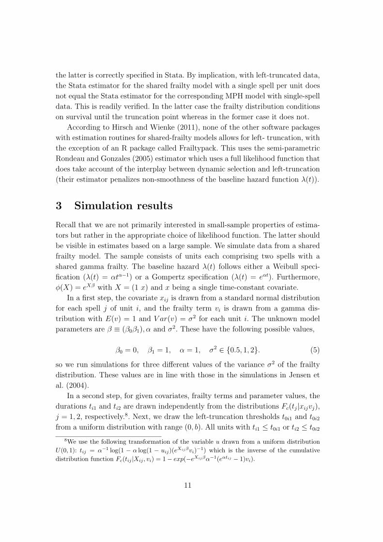
3 Simulation results

Recall that we are not primarily interested in small-sample properties of estima-

tors but rather in the appropriate choice of likelihood function. The latter should

be visible in estimates based on a large sample. We simulate data from a shared

frailty model. The sample consists of units each comprising two spells with a

shared gamma frailty. The baseline hazard λ(t) follows either a Weibull speci-

fication (λ(t) = αtα−1) or a Gompertz specification (λ(t) = eαt). Furthermore,

φ(X) = eXβ with X = (1 x) and x being a single time-constant covariate.

In a first step, the covariate xij is drawn from a standard normal distribution

for each spell j of unit i, and the frailty term vi is drawn from a gamma dis-

tribution with E(v) = 1 and V ar(v) = σ2 for each unit i. The unknown model

parameters are β ≡ (β0β1), α and σ2. These have the following possible values,

β0 = 0, β1 = 1, α = 1, σ2 ∈ {0.5, 1, 2}. (5)

so we run simulations for three different values of the variance σ2 of the frailty

distribution. These values are in line with those in the simulations in Jensen et

al. (2004).

In a second step, for given covariates, frailty terms and parameter values, the

durations ti1 and ti2 are drawn independently from the distributions Fc(tj|xijvj),

j = 1, 2, respectively.8. Next, we draw the left-truncation thresholds t0i1 and t0i2

from a uniform distribution with range (0, b). All units with ti1 ≤ t0i1 or ti2 ≤ t0i2

8We use the following transformation of the variable u drawn from a uniform distributionU(0, 1): tij = α−1 log(1 − α log(1 − uij)(eXijβvi)−1) which is the inverse of the cumulativedistribution function Fc(tij |Xij , vi) = 1− exp(−eXijβα−1(eαtij − 1)vi).

11

are dropped. This way the sample only contains those units for which both spell

durations exceed their left-truncation points. The fraction c ∈ [0, 1] of data that

are dropped due to left-truncation can be fine-tuned by modifying b. Effectively,

the sample size of 50,000 units is determined by the requirement that each of the

spells of these units has a duration exceeding a left-truncation point. In fact, if

the data are sampled from the model with the Weibull specification with α = 1

and if σ2 is large, then the estimation of the parameters β0, α is numerically

cumbersome.9 This suggests that a larger sample is needed for reliable inference,

but in the light of the computational burden we opt for the alternative of assuming

that the researcher knows that β0 = 0.

In the last step of the simulation procedure we use the stset and streg

commands to estimate a shared frailty model in Stata,

. stset duration, failure(cens==0) enter(t0)

. streg x , distribution(gompertz) frailty(gamma) shared(id) nohr

The results are summarized in Figures 1 and 2. The panels show the estimates of

the constant β0 (in the case of the Gompertz specification), the covariate effect

β1, the Gompertz duration dependence parameter α, and the variance σ2 of the

gamma frailty distribution. We performed separate simulations with 30 different

truncation rates c ∈ [0, 1), and we connect the resulting points to obtain the

displayed curves.

All estimates move away from their true value as the truncation rate c in-

creases from zero. In particular, at any positive truncation rate, the covariate

effect and the level of the hazard rate are under-estimated.

In general this is to be expected. As c increases, the simulated distributions

of t0i1 and t0i2 move to the right, so the difference between G(v) and G(v|Ti1 >

t0i1, Ti2 > t0i2, x) increases. Recall that E(v) = 1, whereas with truncation, units

with large v will have exited the state relatively often before having reached

the truncation point, so the mean of v|Ti1 > t0i1, Ti2 > t0i2, x decreases in t0ij.

The over-estimation of the mean frailty among the survivors at the truncation

points is then compensated by an under-estimation of the magnitude of the other

determinants of the level of the individual hazard rate (which by themselves have

increasing effects on the individual hazard rate).

The bias towards zero of the estimate β1 can be explained analogously. The

true frailty distribution after truncation G(v|Ti1 > t0i1, Ti2 > t0i2, x) depends

9More precisely, the estimation routine suffers from occasional numerical problems. Thiseven occurs in the absence of left-truncation (c = 0) if σ2 ≥ 4.

12

.2.4

.6.8

1

0 .2 .4 .6 .8 1

Truncation rate

Var(v)=0.5 Var(v)=1

Var(v)=2

Covariate

.2.4

.6.8

1

0 .2 .4 .6 .8 1

Truncation rate

Var(v)=0.5 Var(v)=1

Var(v)=2

Duration dependence

0.5

11.

52

2.5

0 .2 .4 .6 .8 1

Truncation rate

Var(v)=0.5 Var(v)=1

Var(v)=2

Variance of frailty

Figure 1: Simulation results of a shared gamma frailty model with Weibull du-

ration dependence and left-truncated data using the Stata command streg with

the option shared()

on the covariates x. Spells with a large value of exp(Xijβ as well as a large vi

terminate on average earlier than other spells. So in the case of a positive β1, an

observation in the truncated sample with a large x is more likely to have a small

vi than observations with low x. The association between x and the observed

hazard rates right after the truncation point is therefore smaller than β1. If one

ignores this, by ignoring the dynamic selection before the truncation point, then

the resulting estimate of β1 will be biased towards zero.

It may be instructive to consider some corresponding model expressions in the

case of single-spell duration data. The correct expression for the observed hazard

rate θ(t|T ≥ t0, x) at t ≥ t0 equals

θ(t|T ≥ t0, x) =λ(t) exp(x′β)

1 + σ2 exp(x′β)Λ(t)(6)

13

−2.

5−

2−

1.5

−1

−.5

0

0 .2 .4 .6 .8 1

Truncation rate

Var(v)=0.5 Var(v)=1

Var(v)=2

Constant

.6.7

.8.9

1

0 .2 .4 .6 .8 1

Truncation rate

Var(v)=0.5 Var(v)=1

Var(v)=2

Covariate

.6.7

.8.9

1

0 .2 .4 .6 .8 1

Truncation rate

Var(v)=0.5 Var(v)=1

Var(v)=2

Duration dependence

.51

1.5

22.

5

0 .2 .4 .6 .8 1

Truncation rate

Var(v)=0.5 Var(v)=1

Var(v)=2

Variance of frailty

Figure 2: Simulation results of a shared gamma frailty model with Gompertz

duration dependence and left-truncated data using the Stata command streg

with the option shared()

This does not depend on t0 because the hazard by definition conditions on T ≥ t,

which implies T ≥ t0. The expression for observed hazard assuming that there is

no dynamic selection before t0 is equal to

λ(t) exp(x′β)

1 + σ2 exp(x′β)(Λ(t)− Λ(t0))(7)

The estimates that follow from the latter approach lead to an estimated observed

hazard at t = t0 that fits the corresponding expression of (6) evaluated at the

true parameter values. Hence,

λ̂(t0) exp(x′β̂) = λ(t0) exp(x′β)(1 + σ2 exp(x′β)Λ(t0))−1

For t0 > 0, σ > 0, this leads to the bias implications discussed above.

14

Figures 1 and 2 also show that the bias of the estimates depends on the

variance of the frailty distribution. As the latter increases, the estimates of the

hazard level and the covariate effect move further away from their true values.

Again, this is what would be expected. Notice that none of the biases vanishes

for the sample size n →∞ for a given truncation rate.

It should be kept in mind that the simulation results in Figures 1 and 2 depend

on the choice of baseline hazard and on the gamma frailty distribution as well as

on the choice of the parameter values. For different models the magnitude of the

bias may differ from the presented results.

For Stata users who wish to avoid misspecification of the likelihood function

when estimating shared frailty models with left-truncated duration data, we pro-

grammed the Stata command stregshared, implementing the changes to the

likelihood discussed in Section 2. In the appendix we give a short description

of this new command. Simulations using stregshared confirm that the estima-

tor is correct and that the estimates converge to their true values as n → ∞independent of the level of truncation.

As noted in the previous section, the Stata stcox command allows for semi-

parametric estimation of the shared gamma frailty model with left-truncated

data. We use this routine to estimate this model with the simulated data. This

does not impose the Weibull or Gompertz functional form for the duration de-

pendence λ, and hence standard errors are larger than above. However, with our

sample size, point estimates should be close to their asymptotic values. Instead,

it turns out that the estimates are similar to those obtained with the appropri-

ate streg command, for all values of c considered. This confirms our conjecture

that the stcox command in the case of the shared gamma frailty model with

left-truncated data is programmed on the basis of the LStata likelihood as defined

in the previous section.

This result is of particular interest as the Stata stcox model has been fre-

quently used in the empirical literature to estimate shared gamma frailty models,

and sometimes the data are left-truncated. Gottard and Rampichini (2006) study

the effects of poverty on time to childbirth among young women in Bolivia. In

their data, individuals within a region are assumed to share their frailty term, and

individuals are only included in their sample if they have reached at least the age

of 14 at the time of the survey in 1998. Hence, left-truncation points vary across

individuals. They state that they use the stcox, shared command in their em-

pirical analysis. Studenski et al. (2011), who study the effect of gait speed on

survival among elderly individuals, provide another example. They use data from

9 different cohort studies, and in a sensitivity analysis of their main results, they

15

estimate shared gamma frailty models with Stata, where the frailty is taken to be

cohort-study-specific. The individual lifetime durations are left-truncated by the

entry age into the study. Hemmelgarn et al. (2007) study multidisciplinary care

for elderly patients with chronic kidney disease and its effect on survival. They

assume shared frailties for matched treated and untreated individuals, and they

estimate shared frailty models with Stata and/or SAS. Their data are subject to

left-truncation. Matching on age ensures that both lifetimes durations need to

exceed a left-truncation point in order for the pair to be included in the sample.

4 Conclusion

This paper analyzes the implications of ignoring the effect of left-truncation of

duration data on the distribution of unit-specific unobserved determinants in the

sample, if multiple durations are observed per unit. In the presence of unobserved

heterogeneity, it is vital to correctly account for the truncation that influences

the composition of survivors in the sample, especially if the truncation thresholds

vary across units.

Stata users estimating shared frailty models with the streg or stcox com-

mand need to be aware that with left-truncated data, the estimators of the covari-

ate effects, the duration dependence and the variance of the frailty distribution

may be inconsistent. The magnitude of the bias depends on the level of trunca-

tion and also on the variance of the frailty distribution of the data generating

process. The good news is the fact that the parameter estimates for the covariate

effects are typically biased towards zero. So in the worst case, effects have been

underestimated by Stata.

16

References

Abbring, J.H. and G.J. van den Berg (2007), “The unobserved heterogeneity

distribution in duration analysis”, Biometrika, 94, 87–99.

Chamberlain, G. (1985), “Heterogeneity, omitted variable bias, and duration de-

pendence”, in J.J. Heckman and B. Singer, editors, Longitudinal analysis of

labor market data, Cambridge University Press, Cambridge.

Clayton, D. (1978), “A model for association in bivariate life tables and its ap-

plication in epidemiological studies of familial tendency in chronic disease in-

cidence”, Biometrika, 65, 141–151.

Cleves, M.A., W.W. Gould and RG. Gutierrez (2004), An Introduction to Survival

Analysis Using Stata, Stata Press, College Station.

Do, P. and S. Ma (2010), “Frailty model with spline estimated nonparametric

hazard function”, Statistica Sinica, 20, 561–580.

Gottard, A. and C. Rampichini (2006), “Shared frailty graphical survival mod-

els”, Conference paper, International Conference on Statistical Latent Vari-

ables Models in the Health Sciences.

Guo, G. (1993), “Event-history analysis for left-truncated data”, Sociological

Methodology, 23, 217–243.

Gutierrez, R.G. (2002), “Parametric frailty and shared frailty survival models”,

The Stata Journal, 2, 22–44.

Hemmelgarn, B.R., B.J. Manns, J. Zhang, M. Tonelli, S. Klarenbach, M. Walsh et

al. (2007), “Association between multidisciplinary care and survival for elderly

patients with chronic kidney disease”, Journal of the American Society of

Nephrology, 18, 993–999.

Hirsch, K. and A. Wienke (2011), “Software for semiparametric shared gamma

and log-normal frailty models: An overview”, Computer Methods and Programs

in Biomedicine, forthcoming.

Hougaard, P. (2000) Analysis of Multivariate Survival Data, Springer, Heidelberg.

Jensen, H., R. Brookmeyer, P. Aaby and P.K. Andersen (2004), “Shared frailty

model for left-truncated multivariate survival data”, Working paper, Univer-

sity of Copenhagen.

Kalbfleisch, J.D. and R.L. Prentice (1980), The Statistical Analysis of Failure

Time Data, Wiley, New York.

17

Lancaster, T. (1990), The Econometric Analysis of Transition Data, Cambridge

University Press, Cambridge.

Nielsen, G.G., R.D. Gill, P.K. Andersen, and T.I.A. Sørensen (1992), “A count-

ing process approach to maximum likelihood estimation in frailty models”,

Scandinavian Journal of Statistics, 19, 25–43.

Ridder, G. (1984), “The distribution of single-spell duration data”, in G.R. Neu-

mann and N. Westerg̊ard-Nielsen, editors, Studies in Labor Market Dynamics,

Springer-Verlag, Heidelberg.

Ridder, G. and I. Tunalı (1999), “Stratified partial likelihood estimation”, Journal

of Econometrics, 92, 193–232.

Rondeau, V. and J.R. Gonzalez (2005), “Frailtypack: a computer program for the

analysis of correlated failure time data using penalized likelihood estimation”,

Computational Methods and Programs in Biomedicine, 80, 154–164.

Stata (2009), Stata Survival Analysis and Epidemiological Tables, Reference Man-

ual Release 11, Stata Press, College Station.

Studenski, S., S. Perera, K. Patel, C. Rosano, K. Faulkner, M. Inzitari et al.

(2011), “Gait speed and survival in older adults”, Journal of the American

Medical Association, 305, 50–58.

Therneau, T.M. and P.M. Grambsch (2000), Modeling Survival Data, Springer,

New York.

Van den Berg, G.J. (2001), “Duration models: specification, identification, and

multiple durations”, in: J.J. Heckman and E. Leamer (eds.), Handbook of

Econometrics, Volume V, North-Holland, Amsterdam.

18

Appendix

First, note that the gamma and Inverse-Gaussian distributions are both special

cases of the non-negative exponential family with density

f(v) = vδe−λvm(v)φ(δ, λ)−1. (8)

A shared frailty model with a frailty distribution of this family has the following

survival function (see Hougaard, 2000):

S(t1, t2|x) =

∫ ∞

0

vδe−(λ+M(t1,t2))vm(v) dv1

φ(δ, λ)

=φ(δ, λ + M(t1, t2))

φ(δ, λ), (9)

with M(t1, t2) = φ(x1)Λ(t1) + φ(x2)Λ(t2). The second equality follows from the

fact that (8) is equivalent to φ(δ, λ) =∫∞0

vδe−λvm(v) dv and therefore φ(δ, λ +

M(t1, t2)) =∫∞0

vδe−(λ+M(t1,t2))vm(v) dv.

A Gamma frailty

Let us assume a gamma distributed frailty with E(v) = 1 and V ar(v) = σ2. This

implies the following restrictions on the density function in (8)

δ = 1/σ2 − 1, λ = 1/σ2, m(v) = 1, φ(δ, λ) = λ−(δ+1)Γ(δ + 1), (10)

where Γ(σ2) is the gamma function. Substituting the expression for φ(δ, λ) into

the right hand side of equation (9) leads to

S(t1, t2|x) =(1/σ2 + M(t1, t2))

−1/σ2Γ(1/σ2)

1/σ2−1/σ2

Γ(1/σ2)

= (1 + σ2M(t1, t2))−1/σ2

. (11)

Since f(t1, t2|x) = ∂2(1−S(t1,t2|x))∂t1∂t2

it follows

f(t1, t2|x) =∂M(t1, t2)

∂t1

∂M(t1, t2)

∂t2(σ2 + 1)(1 + σ2M(t1, t2))

−(1/σ2+2). (12)

Finally, let us consider the likelihood contribution of a group i comprising two

subjects with truncation points t01 and t02 and no censoring. Combining the

results from equation (11) and (12) leads to

f(t1, t2|T1 > t01, T2 > t02, x) =f(t1, t2|x)

S(t01, t02|x)

= φ(x1)λ(t1)φ(x2)λ(t2)(σ2 + 1)(1 + σ2M(t01, t02))

1/σ2

(1 + σ2M(t1, t2))−(1/σ2+2)

which is equation (2) from section 2.

19

B Likelihood in the Stata Manual

The Stata Manual (Stata, 2009, p. 383) presents the following likelihood contri-

bution for a group i of a shared frailty model with a gamma frailty in the case of

no censoring

L = φ(x1)λ(t1)φ(x2)λ(t2)(σ2 + 1)(1 + σ2(M(t1, t2)−M(t01, t02)))

−(1/σ2+2).

Rearranging and choosing δ = 1/σ2 − 1 and λ = 1/σ2 according to (10) yields

L = φ(x1)λ(t1)φ(x2)λ(t2)(λ + M(t1, t2)−M(t01, t02))

−(δ+3)Γ(δ + 3)

(λ)−(δ+1)Γ(δ + 1).

Since we know that φ(δ + 2, λ + x) = (λ + x)−(δ+3)Γ(δ + 3) from (10) and that

φ(δ + 2, λ + x) =∫∞0

vδ+2e−(λ+x)vm(v) dv from equation (9) it follows

L = φ(x1)λ(t1)φ(x2)λ(t2)

∫ ∞

0

v2e−(M(t1,t2)−M(t01,t02))vvδe−λvm(v)

λ−(δ+1)Γ(δ + 1)dv

and once the restrictions (10) for the gamma distribution are imposed again

L =

∫ ∞

0

f(t1, t2|T1 > t01, T2 > t02, x, v) dG(v).

C Inverse-Gaussian frailty

Let us assume Inverse-Gaussian distributed frailty terms. Like with the gamma

frailty, this imposes restrictions on the density in (8)

δ = −1/2, m(v) = ψ1/2π−1/2e−ψv v−1, φ(−1/2, λ) = e−(4ψλ)1/2

.

Assuming ψ = λ gives a mean frailty of 1 and choosing σ2 = 1/(2λ) yields

V ar(v) = σ2. Substituting the expression for φ(δ, λ) into the right hand side of

equation (9) leads to

S(t1, t2|x) =exp(−(4( 1

2σ2 )(1

2σ2 + M(t1, t2)))1/2)

exp(−(4( 12σ2 )2)

12 )

= exp(1/σ2 − 1/σ2(1 + 2σ2M(t1, t2))1/2). (13)

Since f(t1, t2|x) = ∂2(1−S(t1,t2|x))∂t1∂t2

it follows

f(t1, t2|x) =∂M(t1, t2)

∂t1

∂M(t1, t2)

∂t2

(1 + σ2(1 + 2σ2M(t1, t2))− 1

2 )S(t1, t2|x)

1 + 2σ2M(t1, t2). (14)

20

Finally, let us consider the likelihood contribution of a group i comprising two

subjects with truncation points t01 and t02 and no censoring. Combining the

results from equation (13) and (14) leads to

f(t1, t2|T1 > t01, T2 > t02, x) =f(t1, t2|x)

S(t01, t02|x)

= φ(x1)λ(t1)φ(x2)λ(t2)(1 + σ2(1 + 2σ2M(t1, t2))

− 12 ) exp(1/σ2 − 1/σ2(1 + 2σ2M(t1, t2))

1/2)

(1 + 2σ2M(t1, t2)) exp(1/σ2 − 1/σ2(1 + 2σ2M(t01, t02))1/2)

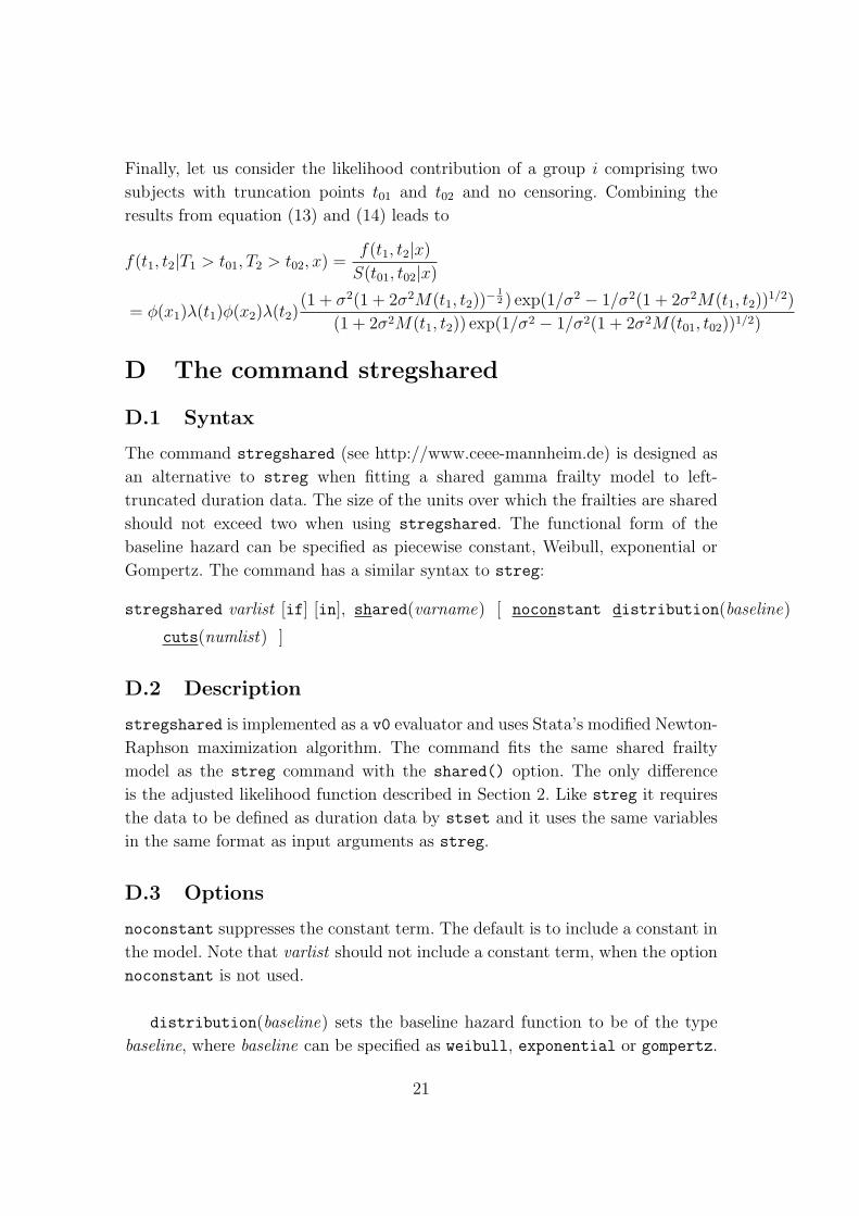
D The command stregshared

D.1 Syntax

The command stregshared (see http://www.ceee-mannheim.de) is designed as

an alternative to streg when fitting a shared gamma frailty model to left-

truncated duration data. The size of the units over which the frailties are shared

should not exceed two when using stregshared. The functional form of the

baseline hazard can be specified as piecewise constant, Weibull, exponential or

Gompertz. The command has a similar syntax to streg:

stregshared varlist [if] [in], shared(varname) [ noconstant distribution(baseline)

cuts(numlist) ]

D.2 Description

stregshared is implemented as a v0 evaluator and uses Stata’s modified Newton-

Raphson maximization algorithm. The command fits the same shared frailty

model as the streg command with the shared() option. The only difference

is the adjusted likelihood function described in Section 2. Like streg it requires

the data to be defined as duration data by stset and it uses the same variables

in the same format as input arguments as streg.

D.3 Options

noconstant suppresses the constant term. The default is to include a constant in

the model. Note that varlist should not include a constant term, when the option

noconstant is not used.

distribution(baseline) sets the baseline hazard function to be of the type

baseline, where baseline can be specified as weibull, exponential or gompertz.

21

If this option is not used, a Weibull model is estimated. Note that the piecewise

constant model requires this option to be specified as d(exponential).

cuts(numlist) specifies the cutoff points of a piecewise constant baseline haz-

ard. When the options noconstant and d(exponential) are used, the option

cuts(numlist ) allows to estimate a piecewise constant model. Here, numlist

holds the list of cutoff points, where the numbers have to be in strictly ascending

order. For example, if the baseline function should be piecewise constant on the

intervals [0, 5.5), [5.5, 10) and [10,∞] use: nocon d(exponential) cuts(5.5,10).

The option cuts() can not be used with d(weibull) or d(gompertz).

shared(varname) specifies a variable defining the units within which the

frailty is shared. The variable in varname is the same variable used in the option

shared of streg. Recall that stregshared can only deal with a unit size of one

or two spells. It is not a problem for the command if some (but not all) of the

units have only one spell and others have two. But it cannot deal with units

holding more than two spells. The shared() option has to be specified.

D.4 Comparison to streg

Since the stregshared command was designed as an alternative to streg, it is

intended to work in a very similar way. So if one uses the original streg Stata

command after stset to estimate a shared gamma-frailty model with a Weibull

distribution

. stset duration, failure(fail == 1) enter(truncation)

. streg x1 x2 x3, shared(id) d(weibull) frailty(gamma) nohr

the same arguments can be used with the stregshared command in order to

estimate the same model with the adjustment in the likelihood function from

Section 2:

. stset duration, failure(fail == 1) enter(truncation)

. stregshared x1 x2 x3, shared(id) d(weibull)

Here, id is the variable that identifies the unit. The same variable is used in the

option shared() in streg. Note that the option nohr which causes streg to

display the estimated parameter values instead of the hazard ratios is not used

in our command. stregshared will display the parameter values as well as the

22

hazard ratios in the estimation results.

In this example the data are left-truncated and therefore the enter(truncation)

option in stset is used, where truncation is the variable that holds the left-

truncation points for each spell. If the enter() option is not used in stset,

stregshared and streg will yield the same estimation results.

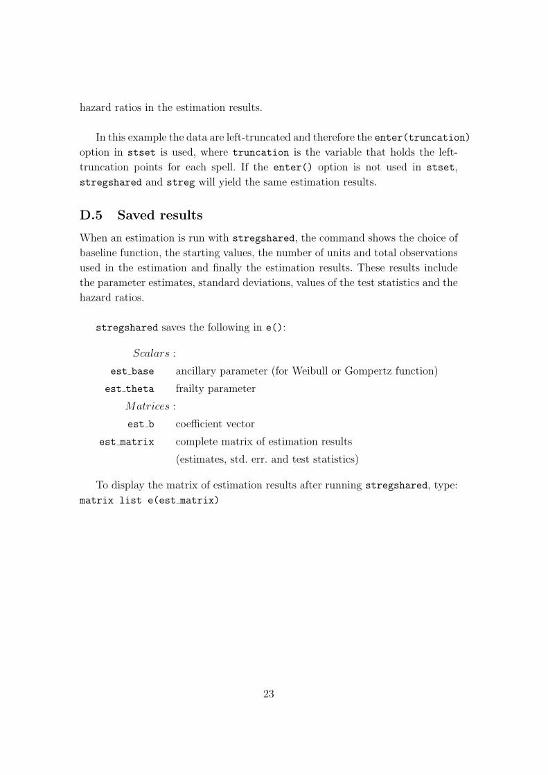
D.5 Saved results

When an estimation is run with stregshared, the command shows the choice of

baseline function, the starting values, the number of units and total observations

used in the estimation and finally the estimation results. These results include

the parameter estimates, standard deviations, values of the test statistics and the

hazard ratios.

stregshared saves the following in e():

Scalars :

est base ancillary parameter (for Weibull or Gompertz function)

est theta frailty parameter

Matrices :

est b coefficient vector

est matrix complete matrix of estimation results

(estimates, std. err. and test statistics)

To display the matrix of estimation results after running stregshared, type:

matrix list e(est matrix)

23