Simultaneous Inference

in General Parametric Models✯

Torsten Hothorn

Institut fur StatistikLudwig-Maximilians-Universitat Munchen

Ludwigstraße 33, D–80539 Munchen, Germany

Frank Bretz

Statistical Methodology, Clinical Information SciencesNovartis Pharma AG

CH-4002 Basel, Switzerland

Peter Westfall

Texas Tech UniversityLubbock, TX 79409, U.S.A

March 4, 2019

Abstract

Simultaneous inference is a common problem in many areas of application. If

multiple null hypotheses are tested simultaneously, the probability of rejecting er-

roneously at least one of them increases beyond the pre-specified significance level.

Simultaneous inference procedures have to be used which adjust for multiplicity and

thus control the overall type I error rate. In this paper we describe simultaneous infer-

ence procedures in general parametric models, where the experimental questions are

specified through a linear combination of elemental model parameters. The frame-

work described here is quite general and extends the canonical theory of multiple

comparison procedures in ANOVA models to linear regression problems, generalized

linear models, linear mixed effects models, the Cox model, robust linear models, etc.

Several examples using a variety of different statistical models illustrate the breadth

✯This is a preprint of an article published in Biometrical Journal, Volume 50, Number 3, 346–363.

Copyright ➞ 2008 WILEY-VCH Verlag GmbH & Co. KGaA, Weinheim; available online http://www.

biometrical-journal.com.

1

of the results. For the analyses we use the R add-on package multcomp, which pro-

vides a convenient interface to the general approach adopted here.

Key words: multiple tests, multiple comparisons, simultaneous confidence intervals,adjusted p-values, multivariate normal distribution, robust statistics.

1 Introduction

Multiplicity is an intrinsic problem of any simultaneous inference. If each of k, say, nullhypotheses is tested at nominal level α, the overall type I error rate can be substantiallylarger than α. That is, the probability of at least one erroneous rejection is larger thanα for k ≥ 2. Common multiple comparison procedures adjust for multiplicity and thusensure that the overall type I error remains below the pre-specified significance level α.Examples of such multiple comparison procedures include Dunnett’s many-to-one compar-isons, Tukey’s all-pairwise comparisons, sequential pairwise contrasts, comparisons withthe average, changepoint analyses, dose-response contrasts, etc. These procedures are allwell established for classical regression and ANOVA models allowing for covariates and/orfactorial treatment structures with i.i.d. normal errors and constant variance, see Bretzet al. (2008) and the references therein. For a general reading on multiple comparisonprocedures we refer to Hochberg and Tamhane (1987) and Hsu (1996).

In this paper we aim at a unified description of simultaneous inference procedures in para-metric models with generally correlated parameter estimates. Each individual null hypothe-sis is specified through a linear combination of elemental model parameters and we allow fork of such null hypotheses to be tested simultaneously, regardless of the number of elementalmodel parameters p. The general framework described here extends the current canoni-cal theory with respect to the following aspects: (i) model assumptions such as normalityand homoscedasticity are relaxed, thus allowing for simultaneous inference in generalizedlinear models, mixed effects models, survival models, etc.; (ii) arbitrary linear functions ofthe elemental parameters are allowed, not just contrasts of means in AN(C)OVA models;(iii) computing the reference distribution is feasible for arbitrary designs, especially forunbalanced designs; and (iv) a unified implementation is provided which allows for a fasttransition of the theoretical results to the desks of data analysts interested in simultaneousinferences for multiple hypotheses.

Accordingly, the paper is organized as follows. Section 2 defines the general model andobtains the asymptotic or exact distribution of linear functions of elemental model parame-ters under rather weak conditions. In Section 3 we describe the framework for simultaneousinference procedures in general parametric models. An overview about important applica-tions of the methodology is given in Section 4 followed by a short discussion of the softwareimplementation in Section 5. Most interesting from a practical point of view is Section 6where we analyze four rather challenging problems with the tools developed in this paper.

2 Model and Parameters

In this section we introduce the underlying model assumptions and derive some asymptoticresults necessary in the subsequent sections. The results from this section form the basisfor the simultaneous inference procedures described in Section 3.

Let M((Z1, . . . ,Zn), θ, η) denote a semi-parametric statistical model. The set of n obser-vations is described by (Z1, . . . ,Zn). The model contains fixed but unknown elementalparameters θ ∈ R

p and other (random or nuisance) parameters η. We are primarily in-terested in the linear functions ϑ := Kθ of the parameter vector θ as specified throughthe constant matrix K ∈ R

k,p. In what follows we describe the underlying model assump-tions, the limiting distribution of estimates of our parameters of interest ϑ, as well as thecorresponding test statistics for hypotheses about ϑ and their limiting joint distribution.

Suppose θn ∈ Rp is an estimate of θ and Sn ∈ R

p,p is an estimate of cov(θn) with

anSnP

−→ Σ ∈ Rp,p (1)

for some positive, nondecreasing sequence an. Furthermore, we assume that a multivariatecentral limit theorem holds, i.e.,

a1/2n (θn − θ)d

−→ Np(0,Σ). (2)

If both (1) and (2) are fulfilled we write θna∼ Np(θ, Sn). Then, by Theorem 3.3.A in Serfling

(1980), the linear function ϑn = Kθn, i.e., an estimate of our parameters of interest, alsofollows an approximate multivariate normal distribution

ϑn = Kθna∼ Nk(ϑ, S

⋆n)

with covariance matrix S⋆n := KSnK

⊤ for any fixed matrix K ∈ Rk,p. Thus we need not

to distinguish between elemental parameters θ or derived parameters ϑ = Kθ that are ofinterest to the researcher. Instead we simply assume for the moment that we have (inanalogy to (1) and (2))

ϑna∼ Nk(ϑ, S

⋆n) with anS

⋆n

P−→ Σ⋆ := KΣK⊤ ∈ R

k,k (3)

and that the k parameters in ϑ are themselves the parameters of interest to the researcher.It is assumed that the diagonal elements of the covariance matrix are positive, i.e., Σ⋆

jj > 0for j = 1, . . . , k.

Then, the standardized estimator ϑn is again asymptotically normally distributed

Tn := D−1/2n (ϑn − ϑ)

a∼ Nk(0,Rn) (4)

where Dn = diag(S⋆n) is the diagonal matrix given by the diagonal elements of S⋆

n and

Rn = D−1/2n S

⋆nD

−1/2n ∈ R

k,k

1

is the correlation matrix of the k-dimensional statistic Tn. To demonstrate (4), note that

with (3) we have anS⋆n

P−→ Σ⋆ and anDn

P−→ diag(Σ⋆). Define the sequence an needed to

establish a-convergence in (4) by an ≡ 1. Then we have

anRn = D−1/2n S

⋆nD

−1/2n

= (anDn)−1/2(anS

⋆n)(anDn)

−1/2

P−→ diag(Σ⋆)−1/2 Σ⋆ diag(Σ⋆)−1/2 =: R ∈ R

k,k

where the convergence in probability to a constant follows from Slutzky’s Theorem (The-orem 1.5.4, Serfling, 1980) and therefore (4) holds. To finish note that

Tn = D−1/2n (ϑn − ϑ) = (anDn)

−1/2a1/2n (ϑn − ϑ)d

−→ Nk(0,R).

For the purposes of multiple comparisons, we need convergence of multivariate probabilitiescalculated for the vector Tn when Tn is assumed normally distributed with Rn treatedas if it were the true correlation matrix. However, such probabilities P(max(|Tn| ≤ t)

are continuous functions of Rn (and a critical value t) which converge by RnP

−→ R asa consequence of Theorem 1.7 in Serfling (1980). In cases where Tn is assumed multi-variate t distributed with Rn treated as the estimated correlation matrix, we have similarconvergence as the degrees of freedom approach infinity.

Since we only assume that the parameter estimates are asymptotically normally distributedwith a consistent estimate of the associated covariance matrix being available, our frame-work covers a large class of statistical models, including linear regression and ANOVAmodels, generalized linear models, linear mixed effects models, the Cox model, robust lin-ear models, etc. Standard software packages can be used to fit such models and obtainthe estimates θn and Sn which are essentially the only two quantities that are needed forwhat follows in Section 3. It should be noted that the elemental parameters θ are notnecessarily means or differences of means in AN(C)OVA models. Also, we do not restrictour attention to contrasts of such means, but allow for any set of constants leading to thelinear functions ϑ = Kθ of interest. Specific examples for K and θ will be given later inSections 4 and 6.

3 Global and Simultaneous Inference

Based on the results from Section 2, we now focus on the derivation of suitable inferenceprocedures. We start considering the general linear hypothesis (Searle, 1971) formulatedin terms of our parameters of interest ϑ

H0 : ϑ := Kθ = m.

2

Under the conditions of H0 it follows from Section 2 that

Tn = D−1/2n (ϑn −m)

a∼ Nk(0,Rn).

This approximating distribution will now be used as the reference distribution when con-structing the inference procedures. The global hypothesis H0 can be tested using standardglobal tests, such as the F - or the χ2-test. An alternative approach is to use maximumtests, as explained in Subsection 3.1. Note that a small global p-value (obtained from oneof these procedures) leading to a rejection of H0 does not give further indication aboutthe nature of the significant result. Therefore, one is often interested in the individual nullhypotheses

Hj0 : ϑj = mj.

Testing the hypotheses set {H10 , . . . , H

k0 } simultaneously thus requires the individual as-

sessments while maintaining the familywise error rate, as discussed in Subsection 3.2

At this point it is worth considering two special cases. A stronger assumption than asymp-totic normality of θn in (2) is exact normality, i.e., θn ∼ Np(θ,Σ). If the covariance matrixΣ is known, it follows by standard arguments that Tn ∼ Nk(0,R), when Tn is normalizedusing fixed, known variances. Otherwise, in the typical situation of linear models withnormal i.i.d. errors, Σ = σ2A, where σ2 is unknown but A is fixed and known, the exactdistribution of Tn is a k-dimensional multivariate tk(ν,R) distribution with ν degrees offreedom (ν = n− p− 1 for linear models), see Tong (1990).

3.1 Global Inference

The F - and the χ2-test are classical approaches to assess the global null hypothesis H0.Standard results (such as Theorem 3.5, Serfling, 1980) ensure that

X2 = T⊤

nR+nTn

d−→ χ2(Rank(R)) when θn

a∼ Np(θ, Sn)

F =T⊤

nR+Tn

Rank(R)∼ F(Rank(R), ν) when θn ∼ Np(θ, σ

2A),

where Rank(R) and ν are the corresponding degrees of freedom of the χ2 and F distri-bution, respectively. Furthermore, Rank(Rn)

+ denotes the Moore-Penrose inverse of thecorrelation matrix Rank(R).

Another suitable scalar test statistic for testing the global hypothesis H0 is to considerthe maximum of the individual test statistics T1,n, . . . , Tk,n of the multivariate statisticTn = (T1,n, . . . , Tk,n), leading to a max-t type test statistic max(|Tn|). The distributionof this statistic under the conditions of H0 can be handled through the k-dimensionaldistribution

P(max(|Tn|) ≤ t) ∼=

t∫

−t

· · ·

t∫

−t

ϕk(x1, . . . , xk;R, ν) dx1 · · · dxk =: gν(R, t) (5)

3

for some t ∈ R, where ϕk is the density function of either the limiting k-dimensionalmultivariate normal (with ν = ∞ and the ‘≈’ operator) or the exact multivariate tk(ν,R)-distribution (with ν < ∞ and the ‘=’ operator). Since R is usually unknown, we plug-inthe consistent estimate Rn as discussed in Section 2. The resulting global p-value (exactor approximate, depending on context) for H0 is 1 − gν(Rn,max |t|) when T = t hasbeen observed. Efficient methods for approximating the above multivariate normal andt integrals are described in Genz (1992); Genz and Bretz (1999); Bretz et al. (2001) andGenz and Bretz (2002).

In contrast to the global F - or χ2-test, the max-t test based on the test statistic max(|Tn|)also provides information, which of the k individual null hypotheses H

j0 , j = 1, . . . , k is

significant, as well as simultaneous confidence intervals, as shown in the next subsection.

3.2 Simultaneous Inference

We now consider testing the k null hypotheses H10 , . . . , H

k0 individually and require that

the familywise error rate, i.e., the probability of falsely rejecting at least one true nullhypothesis, is bounded by the nominal significance level α ∈ (0, 1). In what follows weuse adjusted p-values to describe the decision rules. Adjusted p-values are defined as thesmallest significance level for which one still rejects an individual hypothesis H

j0 , given a

particular multiple test procedure. In the present context of single-step tests, the (at leastasymptotic) adjusted p-value for the jth individual two-sided hypothesis Hj

0 : ϑj = mj, j =1, . . . , k, is given by

pj = 1− gν(Rn, |tj|),

where t1, . . . , tk denote the observed test statistics. By construction, we can reject anindividual null hypothesis H

j0 , j = 1, . . . , k, whenever the associated adjusted p-value is

less than or equal to the pre-specified significance level α, i.e., pj ≤ α. The adjustedp-values are calculated from expression (5).

Similar results also hold for one-sided testing problems. The adjusted p-values for one-sided cases are defined analogously, using one-sided multidimensional integrals instead ofthe two-sided integrals (5). Again, we refer to Genz (1992); Genz and Bretz (1999); Bretzet al. (2001) and Genz and Bretz (2002) for the numerical details.

In addition to a simultaneous test procedure, a (at least approximate) simultaneous (1 −2α)× 100% confidence interval for ϑ is given by

ϑn ± qαD1/2n

where qα is the 1 − α quantile of the distribution (asymptotic, if necessary) of Tn. Thisquantile can be calculated or approximated via (5), i.e., qα is chosen such that gν(Rn, qα) =1− α. The corresponding one-sided versions are defined analogously.

4

It should be noted that the simultaneous inference procedures described so far belong tothe class of single-step procedures, since a common critical value qα is used for the indi-vidual tests. Single-step procedures have the advantage that corresponding simultaneousconfidence intervals are easily available, as previously noted. However, single-step proce-dures can always be improved by stepwise extensions based on the closed test procedure.That is, for a given family of null hypotheses H1

0 , . . . , Hk0 , an individual hypothesis Hj

0 isrejected only if all intersection hypotheses HJ =

⋂

i∈J Hi0 with j ∈ J ⊆ {1, . . . , k} are

rejected (Marcus et al., 1976). Such stepwise extensions can thus be applied to any of themethods discussed in this paper, see for example Westfall (1997) and Westfall and Tobias(2007).

4 Applications

The methodological framework described in Sections 2 and 3 is very general and thusapplicable to a wide range of statistical models. Many estimation techniques, such as(restricted) maximum likelihood and M-estimation, provide at least asymptotically normalestimates of the elemental parameters together with consistent estimates of their covariancematrix. In this section we illustrate the generality of the methodology by reviewing somepotential applications. Detailed numerical examples are discussed in Section 6. In whatfollows, we assume m = 0 only for the sake of simplicity. The next paragraphs highlight asubjective selection of some special cases of practical importance.

Multiple Linear Regression. In standard regression models the observations Zi ofsubject i = 1, . . . , n consist of a response variable Yi and a vector of covariates Xi =(Xi1, . . . , Xiq), such that Zi = (Yi,Xi) and p = q+1. The response is modelled by a linearcombination of the covariates with normal error εi and constant variance σ2,

Yi = β0 +

q∑

j=1

βjXij + σεi,

where ε = (ε1, . . . , εn)⊤ ∼ Nn(0, In). The elemental parameter vector is θ = (β0, β1, . . . , βq),

which is usually estimated by

θn =(

X⊤X)−1

X⊤Y ∼ Nq+1

(

θ, σ2(

X⊤X)−1

)

,

where Y = (Y1, . . . , Yn) denotes the response vector and X = (1, (Xij))ij denotes thedesign matrix, i = 1, . . . , n, j = 1, . . . , q. Thus, for every matrix K ∈ R

k,q+1 of constantsdetermining the experimental questions of interest we have

ϑn = Kθn ∼ Nk(Kθ, σ2K(

X⊤X)−1

K⊤).

5

Under the null hypothesis ϑ = 0 the standardized test statistic follows a multivariate t

distribution

Tn = D−1/2n ϑn ∼ tq+1(n− q,R),

where Dn = σ2diag(K(

X⊤X)−1

K⊤) is the diagonal matrix of the estimated variances of

Kθ and R is the correlation matrix as given in Section 3. The body fat prediction examplepresented in Subsection 6.2 illustrates the application of simultaneous inference proceduresin the context of variable selection in linear regression models.

One-way ANOVA. Consider a one-way ANOVA model for a factor measured at q levelswith a continuous response

Yij = µ+ γj + εij (6)

and independent normal errors εij ∼ N1(0, σ2), j = 1, . . . , q, i = 1, . . . , nj. Note that

the model description in (6) is overparameterized. A standard approach is to consider asuitable re-parametrization. The so-called ”treatment contrast” vector θ = (µ, γ2− γ1, γ3−γ1, . . . , γq−γ1) is, for example, the default re-parametrization used as elemental parametersin the R-system for statistical computing (R Development Core Team, 2008).

Many classical multiple comparison procedures can be embedded into this framework,including Dunnett’s many-to-one comparisons and Tukey’s all-pairwise comparisons. ForDunnett’s procedure, the differences γj−γ1 are tested for all j = 2, . . . , q, where γ1 denotesthe mean treatment effect of a control group. In the notation from Section 2 we thus have

KDunnett = (0, diag(q))

resulting in the parameters of interest

ϑDunnett = KDunnettθ = (γ2 − γ1, γ3 − γ1, . . . , γq − γ1)

of interest. For Tukey’s procedure, the interest is in all-pairwise comparisons of the pa-rameters γ1, . . . , γq. For q = 3, for example, we have

KTukey =

0 1 00 0 10 1 −1

with parameters of interest

ϑTukey = KTukeyθ = (γ2 − γ1, γ3 − γ1, γ2 − γ3).

Many further multiple comparison procedures have been investigated in the past, whichall fit into this framework. We refer to Bretz et al. (2001) for a related comprehensive list.

6

Note that under the standard ANOVA assumptions of i.i.d. normal errors with constantvariance the vector of test statistics Tn follows a multivariate t distribution. Thus, relatedsimultaneous tests and confidence intervals do not rely on asymptotics and can be computedanalytically instead, as shown in Section 3. To illustrate simultaneous inference proceduresin one-way ANOVA models, we consider all pairwise comparisons of expression levels forvarious genetic conditions of alcoholism in Subsection 6.1.

Further parametric models. In generalized linear models, the exact distribution of theparameter estimates is usually unknown and thus the asymptotic normal distribution is thebasis for all inference procedures. When we are interested in inference about model param-eters corresponding to levels of a certain factor, the same multiple comparison proceduresas sketched above are available.

Linear and non-linear mixed effects models fitted by restricted maximum-likelihood pro-vide the data analyst with asymptotically normal estimates and a consistent covariancematrix as well so that all assumptions of our framework are met and one can set up simul-taneous inference procedures for these models as well. The same is true for the Cox model

or other parametric survival models such as the Weibull model.

We use logistic regression models to estimated the probability of suffering from Alzheimer’sdisease in Subsection 6.3, compare several risk factors for survival of leukemia patientsby means of a Weibull model in Subsection 6.4 and obtain probability estimates of deerbrowsing for various tree species from mixed models in Subsection 6.5.

Robust simultaneous inference. Yet another application is to use robust variantsof the previously discussed statistical models. One possibility is to consider the use ofsandwich estimators Sn for the covariance matrix cov(θn) when, for example, the vari-ance homogeneity assumption is violated. An alternative is to apply robust estimationtechniques in linear models, for example S-, M- or MM-estimation (see Rousseeuw andLeroy, 2003; Stefanski and Boos, 2002; Yohai, 1987, for example), which again provide uswith asymptotically normal estimates. The reader is referred to Subsection 6.2 for somenumerical examples illustrating these ideas.

5 Implementation

The multcomp package (Hothorn et al., 2008) in R (R Development Core Team, 2008)provides a general implementation of the framework for simultaneous inference in semi-parametric models described in Sections 2 and 3. The numerical examples in Section 6 willall be analyzed using the multcomp package. In this section we briefly introduce the user-interface and refer the reader to the online documentation of the package for the technicaldetails.

7

Estimated model coefficients θn and their estimated covariance matrix Sn are accessible inR via coef() and vcov()methods available for most statistical models in R, such as objectsof class lm, glm, coxph, nlme, mer or survreg. Having this information at hand, the glht()function sets up the general linear hypothesis for a model ‘model’ and a representation ofthe matrix K (via its linfct argument):

glht(model, linfct, alternative = c("two.sided", "less", "greater"),

rhs = 0, ...)

The two remaining arguments alternative and rhs define the direction of the alternative(see Section 3) and m, respectively.

The matrix K can be described in three different ways:

❼ by a matrix with length(coef(model)) columns, or

❼ by an expression or character vector giving a symbolic description of the linear func-tions of interest, or

❼ by an object of class mcp (for multiple comparison procedure).

The last alternative is convenient when contrasts of factor levels are to be compared andthe model contrasts used to define the design matrix of the model have to be taken intoaccount. The mcp() function takes the name of the factor to be tested as an argument aswell as a character defining the type of comparisons as its value. For example, mcp(treat= "Tukey") sets up a matrix K for Tukey’s all-pairwise comparisons among the levels ofthe factor treat, which has to appear on right hand side of the model formula of model. Inthis particular case, we need to assume that model.frame() and model.matrix() methodsfor model are available as well.

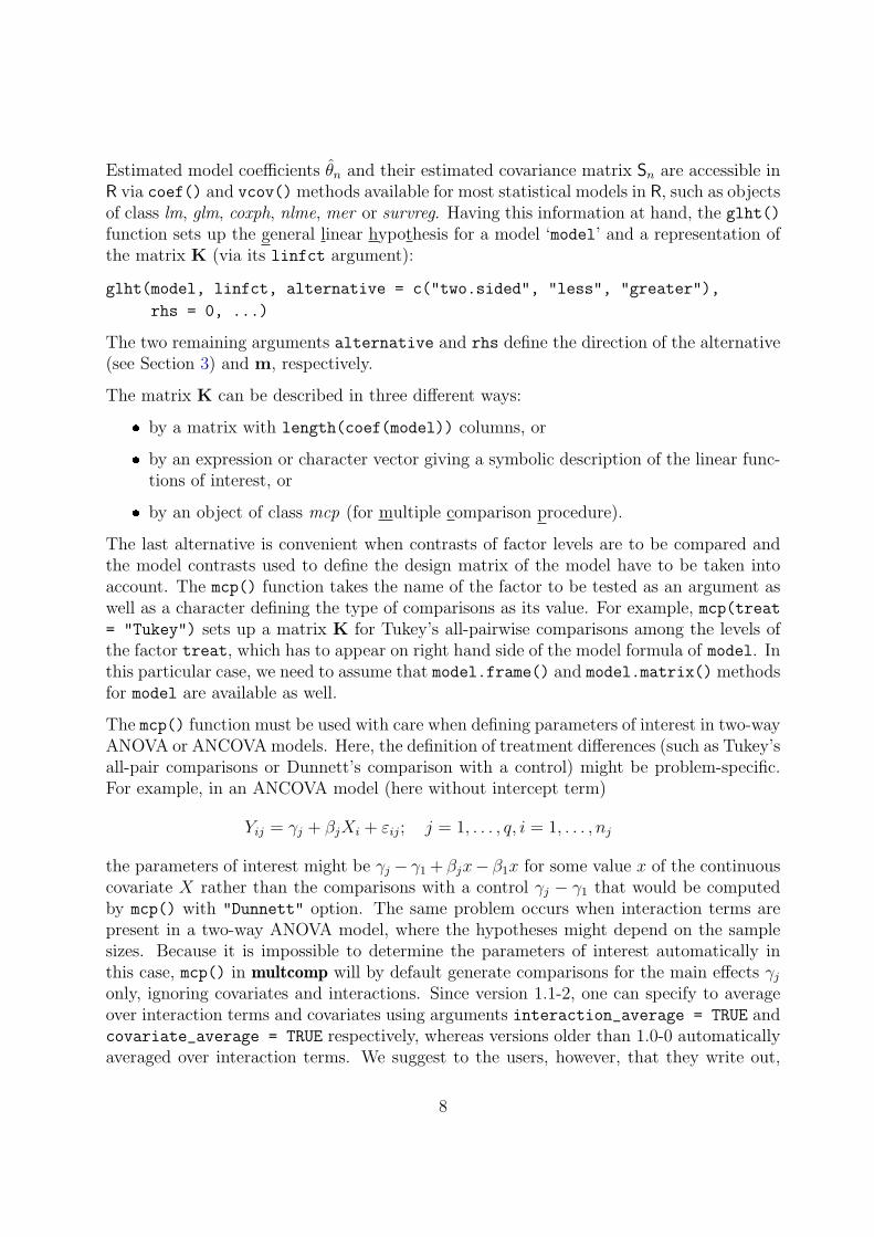
The mcp() function must be used with care when defining parameters of interest in two-wayANOVA or ANCOVA models. Here, the definition of treatment differences (such as Tukey’sall-pair comparisons or Dunnett’s comparison with a control) might be problem-specific.For example, in an ANCOVA model (here without intercept term)

Yij = γj + βjXi + εij; j = 1, . . . , q, i = 1, . . . , nj

the parameters of interest might be γj − γ1 + βjx− β1x for some value x of the continuouscovariate X rather than the comparisons with a control γj − γ1 that would be computedby mcp() with "Dunnett" option. The same problem occurs when interaction terms arepresent in a two-way ANOVA model, where the hypotheses might depend on the samplesizes. Because it is impossible to determine the parameters of interest automatically inthis case, mcp() in multcomp will by default generate comparisons for the main effects γjonly, ignoring covariates and interactions. Since version 1.1-2, one can specify to averageover interaction terms and covariates using arguments interaction_average = TRUE andcovariate_average = TRUE respectively, whereas versions older than 1.0-0 automaticallyaveraged over interaction terms. We suggest to the users, however, that they write out,

8

manually, the set of contrasts they want. One should do this whenever there is doubt aboutwhat the default contrasts measure, which typically happens in models with higher orderinteraction terms. We refer to Hsu (1996), Chapter 7, and Searle (1971), Chapter 7.3, forfurther discussions and examples on this issue.

Objects of class glht returned by glht() include coef() and vcov() methods to computeϑn and S

⋆n. Furthermore, a summary() method is available to perform different tests (max

t, χ2 and F -tests) and p-value adjustments, including those taking logical constraints intoaccount (Shaffer, 1986; Westfall, 1997). In addition, the confint() method applied toobjects of class glht returns simultaneous confidence intervals and allows for a graphicalrepresentation of the results. The numerical accuracy of adjusted p-values and simultane-ous confidence intervals implemented in multcomp is continuously checked against resultsreported by Westfall et al. (1999).

6 Illustrations

6.1 Genetic Components of Alcoholism

Various studies have linked alcohol dependence phenotypes to chromosome 4. One can-didate gene is NACP (non-amyloid component of plaques), coding for alpha synuclein.Bonsch et al. (2005) found longer alleles of NACP -REP1 in alcohol-dependent patientscompared with healthy controls and report that the allele lengths show some associationwith levels of expressed alpha synuclein mRNA in alcohol-dependent subjects (see Fig-ure 1). Allele length is measured as a sum score built from additive dinucleotide repeatlength and categorized into three groups: short (0 − 4, n = 24), intermediate (5 − 9,n = 58), and long (10 − 12, n = 15). The data are available from package coin. Here,we are interested in comparing the distribution of the expression level of alpha synucleinmRNA in three groups of subjects defined by the allele length.

Thus, we fit a simple one-way ANOVA model to the data and define K such that Kθ

contains all three group differences (Tukey’s all-pairwise comparisons):

R> data("alpha", package = "coin")

R> amod <- aov(elevel ~ alength, data = alpha)

R> amod_glht <- glht(amod, linfct = mcp(alength = "Tukey"))

R> amod_glht$linfct

(Intercept) alengthintermediate alengthlong

intermediate - short 0 1 0

long - short 0 0 1

long - intermediate 0 -1 1

attr(,"type")

[1] "Tukey"

9

●

●●

●

●●

short intermediate long

−2

02

46

NACP−REP1 Allele Length

Exp

ressio

n L

eve

l

n = 24 n = 58 n = 15

Figure 1: alpha data: Distribution of levels of expressed alpha synuclein mRNA in threegroups defined by the NACP -REP1 allele lengths.

The amod_glht object now contains information about the estimated linear function ϑn

and their covariance matrix S⋆n which can be inspected via the coef() and vcov()methods:

R> coef(amod_glht)

intermediate - short long - short long - intermediate

0.4341523 1.1887500 0.7545977

R> vcov(amod_glht)

intermediate - short long - short long - intermediate

intermediate - short 0.14717604 0.1041001 -0.04307591

long - short 0.10410012 0.2706603 0.16656020

long - intermediate -0.04307591 0.1665602 0.20963611

The summary() and confint() methods can be used to compute a summary statisticincluding adjusted p-values and simultaneous confidence intervals, respectively:

R> confint(amod_glht)

Simultaneous Confidence Intervals

Multiple Comparisons of Means: Tukey Contrasts

Fit: aov(formula = elevel ~ alength, data = alpha)

Quantile = 2.3717

95% family-wise confidence level

10

Linear Hypotheses:

Estimate lwr upr

intermediate - short == 0 0.43415 -0.47572 1.34402

long - short == 0 1.18875 -0.04513 2.42263

long - intermediate == 0 0.75460 -0.33132 1.84051

R> summary(amod_glht)

Simultaneous Tests for General Linear Hypotheses

Multiple Comparisons of Means: Tukey Contrasts

Fit: aov(formula = elevel ~ alength, data = alpha)

Linear Hypotheses:

Estimate Std. Error t value Pr(>|t|)

intermediate - short == 0 0.4342 0.3836 1.132 0.4924

long - short == 0 1.1888 0.5203 2.285 0.0614 .

long - intermediate == 0 0.7546 0.4579 1.648 0.2270

---

Signif. codes: 0 ‘***’ 0.001 ‘**’ 0.01 ‘*’ 0.05 ‘.’ 0.1 ‘ ’ 1

(Adjusted p values reported -- single-step method)

Because of the variance heterogeneity that can be observed in Figure 1, one might beconcerned with the validity of the above results stating that there is no difference betweenany combination of the three allele lengths. A sandwich estimator Sn might be moreappropriate in this situation, and the vcov argument can be used to specify a function tocompute some alternative covariance estimator Sn as follows:

R> amod_glht_sw <- glht(amod, linfct = mcp(alength = "Tukey"),

+ vcov = sandwich)

R> summary(amod_glht_sw)

Simultaneous Tests for General Linear Hypotheses

Multiple Comparisons of Means: Tukey Contrasts

Fit: aov(formula = elevel ~ alength, data = alpha)

Linear Hypotheses:

Estimate Std. Error t value Pr(>|t|)

intermediate - short == 0 0.4342 0.4239 1.024 0.5594

long - short == 0 1.1888 0.4432 2.682 0.0227 *

long - intermediate == 0 0.7546 0.3184 2.370 0.0502 .

---

Signif. codes: 0 ‘***’ 0.001 ‘**’ 0.01 ‘*’ 0.05 ‘.’ 0.1 ‘ ’ 1

11

(Adjusted p values reported -- single-step method)

We used the sandwich() function from package sandwich (Zeileis, 2004, 2006) which pro-vides us with a heteroscedasticity-consistent estimator of the covariance matrix. Thisresult is more in line with previously published findings for this study obtained from non-parametric test procedures such as the Kruskal-Wallis test. A comparison of the simul-taneous confidence intervals calculated based on the ordinary and sandwich estimator isgiven in Figure 2.

Tukey (ordinary Sn)

−0.5 0.5 1.5 2.5

long − intermediate

long − short

intermediate − short (

(

(

)

)

)

●

●

●

Difference

Tukey (sandwich Sn)

−0.5 0.5 1.5 2.5

long − intermediate

long − short

intermediate − short (

(

(

)

)

)

●

●

●

Difference

Figure 2: alpha data: Simultaneous confidence intervals based on the ordinary covariancematrix (left) and a sandwich estimator (right).

6.2 Prediction of Total Body Fat

Garcia et al. (2005) report on the development of predictive regression equations for bodyfat content by means of p = 9 common anthropometric measurements which were obtainedfor n = 71 healthy German women. In addition, the women’s body composition wasmeasured by Dual Energy X-Ray Absorptiometry (DXA). This reference method is veryaccurate in measuring body fat but finds little applicability in practical environments,mainly because of high costs and the methodological efforts needed. Therefore, a simpleregression equation for predicting DXA measurements of body fat is of special interestfor the practitioner. Backward-elimination was applied to select important variables fromthe available anthropometrical measurements and Garcia et al. (2005) report a final linearmodel utilizing hip circumference, knee breadth and a compound covariate which is definedas the sum of log chin skinfold, log triceps skinfold and log subscapular skinfold. Here,we fit the saturated model to the data and use the max-t test over all t-statistics to selectimportant variables based on adjusted p-values. The linear model including all covariatesand the classical unadjusted p-values are given by

12

R> data("bodyfat", package = "TH.data")

R> summary(lmod <- lm(DEXfat ~ ., data = bodyfat))

Call:

lm(formula = DEXfat ~ ., data = bodyfat)

Residuals:

Min 1Q Median 3Q Max

-6.954 -1.949 -0.219 1.169 10.812

Coefficients:

Estimate Std. Error t value Pr(>|t|)

(Intercept) -69.02828 7.51686 -9.183 4.18e-13 ***

age 0.01996 0.03221 0.620 0.53777

waistcirc 0.21049 0.06714 3.135 0.00264 **

hipcirc 0.34351 0.08037 4.274 6.85e-05 ***

elbowbreadth -0.41237 1.02291 -0.403 0.68826

kneebreadth 1.75798 0.72495 2.425 0.01829 *

anthro3a 5.74230 5.20752 1.103 0.27449

anthro3b 9.86643 5.65786 1.744 0.08622 .

anthro3c 0.38743 2.08746 0.186 0.85338

anthro4 -6.57439 6.48918 -1.013 0.31500

---

Signif. codes: 0 ‘***’ 0.001 ‘**’ 0.01 ‘*’ 0.05 ‘.’ 0.1 ‘ ’ 1

Residual standard error: 3.281 on 61 degrees of freedom

Multiple R-squared: 0.9231, Adjusted R-squared: 0.9117

F-statistic: 81.35 on 9 and 61 DF, p-value: < 2.2e-16

The marix of linear functions K is basically the identity matrix, except for the interceptwhich is omitted. Once the matrix K has been defined, it can be used to set up the generallinear hypotheses:

R> K <- cbind(0, diag(length(coef(lmod)) - 1))

R> rownames(K) <- names(coef(lmod))[-1]

R> lmod_glht <- glht(lmod, linfct = K)

Classically, one would perform an F -test to check if any of the regression coefficients isnon-zero:

R> summary(lmod_glht, test = Ftest())

General Linear Hypotheses

Linear Hypotheses:

Estimate

age == 0 0.01996

waistcirc == 0 0.21049

hipcirc == 0 0.34351

elbowbreadth == 0 -0.41237

13

kneebreadth == 0 1.75798

anthro3a == 0 5.74230

anthro3b == 0 9.86643

anthro3c == 0 0.38743

anthro4 == 0 -6.57439

Global Test:

F DF1 DF2 Pr(>F)

1 81.35 9 61 1.387e-30

but the source of the deviation from the global null hypothesis can only be inspected bythe corresponding max-t test, i.e., via

R> summary(lmod_glht)

Simultaneous Tests for General Linear Hypotheses

Fit: lm(formula = DEXfat ~ ., data = bodyfat)

Linear Hypotheses:

Estimate Std. Error t value Pr(>|t|)

age == 0 0.01996 0.03221 0.620 0.9959

waistcirc == 0 0.21049 0.06714 3.135 0.0212 *

hipcirc == 0 0.34351 0.08037 4.274 <0.01 ***

elbowbreadth == 0 -0.41237 1.02291 -0.403 0.9998

kneebreadth == 0 1.75798 0.72495 2.425 0.1321

anthro3a == 0 5.74230 5.20752 1.103 0.8945

anthro3b == 0 9.86643 5.65786 1.744 0.4785

anthro3c == 0 0.38743 2.08746 0.186 1.0000

anthro4 == 0 -6.57439 6.48918 -1.013 0.9297

---

Signif. codes: 0 ‘***’ 0.001 ‘**’ 0.01 ‘*’ 0.05 ‘.’ 0.1 ‘ ’ 1

(Adjusted p values reported -- single-step method)

Only two covariates, waist and hip circumference, seem to be important and caused therejection of H0. Alternatively, an MM-estimator (Yohai, 1987) as implemented by lmrob()

from package lmrob (Todorov et al., 2007) can be used to fit a robust version of the abovelinear model, the results coincide rather nicely (note that the control arguments to lmrob()were changed in multcomp version 1.2-6 and thus the results have slightly changed):

R> summary(glht(lmrob(DEXfat ~ ., data = bodyfat,

+ control = lmrob.control(setting = "KS2011")), linfct = K))

Simultaneous Tests for General Linear Hypotheses

Fit: lmrob(formula = DEXfat ~ ., data = bodyfat, control = lmrob.control(setting = "KS2011"))

Linear Hypotheses:

Estimate Std. Error z value Pr(>|z|)

age == 0 0.02402 0.02503 0.960 0.949

14

waistcirc == 0 0.23332 0.05251 4.443 <0.001 ***

hipcirc == 0 0.32704 0.06284 5.204 <0.001 ***

elbowbreadth == 0 -0.18365 0.80605 -0.228 1.000

kneebreadth == 0 0.93920 0.58119 1.616 0.564

anthro3a == 0 2.39804 4.06965 0.589 0.997

anthro3b == 0 10.43153 4.46856 2.334 0.144

anthro3c == 0 1.51367 1.62734 0.930 0.957

anthro4 == 0 -5.77695 5.11925 -1.128 0.887

---

Signif. codes: 0 ‘***’ 0.001 ‘**’ 0.01 ‘*’ 0.05 ‘.’ 0.1 ‘ ’ 1

(Adjusted p values reported -- single-step method)

and the result reported above holds under very mild model assumptions.

6.3 Smoking and Alzheimer’s Disease

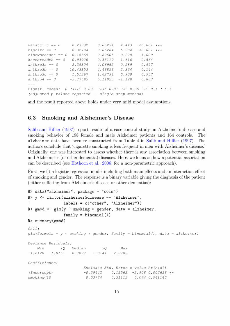
Salib and Hillier (1997) report results of a case-control study on Alzheimer’s disease andsmoking behavior of 198 female and male Alzheimer patients and 164 controls. Thealzheimer data have been re-constructed from Table 4 in Salib and Hillier (1997). Theauthors conclude that ‘cigarette smoking is less frequent in men with Alzheimer’s disease.’Originally, one was interested to assess whether there is any association between smokingand Alzheimer’s (or other dementia) diseases. Here, we focus on how a potential associationcan be described (see Hothorn et al., 2006, for a non-parametric approach).

First, we fit a logistic regression model including both main effects and an interaction effectof smoking and gender. The response is a binary variable giving the diagnosis of the patient(either suffering from Alzheimer’s disease or other dementias):

R> data("alzheimer", package = "coin")

R> y <- factor(alzheimer$disease == "Alzheimer",

+ labels = c("other", "Alzheimer"))

R> gmod <- glm(y ~ smoking * gender, data = alzheimer,

+ family = binomial())

R> summary(gmod)

Call:

glm(formula = y ~ smoking * gender, family = binomial(), data = alzheimer)

Deviance Residuals:

Min 1Q Median 3Q Max

-1.6120 -1.0151 -0.7897 1.3141 2.0782

Coefficients:

Estimate Std. Error z value Pr(>|z|)

(Intercept) -0.39442 0.13563 -2.908 0.003638 **

smoking<10 0.03774 0.51113 0.074 0.941140

15

smoking10-20 -0.61111 0.33084 -1.847 0.064725 .

smoking>20 0.54857 0.34867 1.573 0.115647

genderMale 0.07856 0.26039 0.302 0.762870

smoking<10:genderMale 1.25894 0.87692 1.436 0.151105

smoking10-20:genderMale -0.02855 0.50116 -0.057 0.954568

smoking>20:genderMale -2.26959 0.59948 -3.786 0.000153 ***

---

Signif. codes: 0 ‘***’ 0.001 ‘**’ 0.01 ‘*’ 0.05 ‘.’ 0.1 ‘ ’ 1

(Dispersion parameter for binomial family taken to be 1)

Null deviance: 707.90 on 537 degrees of freedom

Residual deviance: 673.55 on 530 degrees of freedom

AIC: 689.55

Number of Fisher Scoring iterations: 4

The negative regression coefficient for heavy smoking males indicates that Alzheimer’sdisease might be less frequent in this group, but the model is still difficult to interpretbased on the coefficients and corresponding p-values only. Therefore, confidence intervalson the probability scale for the different ‘risk groups’ are interesting and can be computed asfollows. For each combination of gender and smoking behavior, the probability of sufferingfrom Alzheimer’s disease can be estimated by computing the logit function of the linearpredictor from model gmod. Using the predict() method for generalized linear modelsis a convenient way to compute these probability estimates. Alternatively, we can set up

K such that(

1 + exp(−ϑn))−1

is the vector of estimated probabilities with simultaneous

confidence intervals(

(

1 + exp(

−(

ϑn − qαD1/2n

)))−1

,(

1 + exp(

−(

ϑn + qαD1/2n

)))−1)

.

For our model, K is given by the following matrix (essentially the design matrix of gmodfor eight persons with different smoking behavior from both genders)

R> K

(Icpt) s<10 s10-20 s>20 gMale s<10:gMale s10-20:gMale s>20:gMale

None:Female 1 0 0 0 0 0 0 0

<10:Female 1 1 0 0 0 0 0 0

10-20:Female 1 0 1 0 0 0 0 0

>20:Female 1 0 0 1 0 0 0 0

None:Male 1 0 0 0 1 0 0 0

<10:Male 1 1 0 0 1 1 0 0

10-20:Male 1 0 1 0 1 0 1 0

>20:Male 1 0 0 1 1 0 0 1

and can easily be used to compute the confidence intervals described above

16

R> gmod_ci <- confint(glht(gmod, linfct = K))

R> gmod_ci$confint <- apply(gmod_ci$confint, 2, binomial()$linkinv)

R> plot(gmod_ci, xlab = "Probability of Developing Alzheimer",

+ xlim = c(0, 1))

The simultaneous confidence intervals are depicted in Figure 3. Using this representationof the results, it is obvious that Alzheimer’s disease is less frequent in heavy smoking mencompared to all other configurations of the two covariates.

0.0 0.2 0.4 0.6 0.8 1.0

>20:Male

10−20:Male

<10:Male

None:Male

>20:Female

10−20:Female

<10:Female

None:Female (

(

(

(

(

(

(

(

)

)

)

)

)

)

)

)

●

●

●

●

●

●

●

●

Probability of Developing Alzheimer

Figure 3: alzheimer data: Simultaneous confidence intervals for the probability to sufferfrom Alzheimer’s disease.

6.4 Acute Myeloid Leukemia Survival

The treatment of patients suffering from acute myeloid leukemia (AML) is determinedby a tumor classification scheme taking the status of various cytogenetic aberrations intoaccount. Bullinger et al. (2004) investigate an extended tumor classification scheme incor-porating molecular subgroups of the disease obtained by gene expression profiling. Theanalyses reported here are based on clinical data only (thus omitting available gene ex-pression data) published online at http://www.ncbi.nlm.nih.gov/geo, accession numberGSE425. The overall survival time and censoring indicator as well as the clinical variablesage, sex, lactic dehydrogenase level (LDH), white blood cell count (WBC), and treatmentgroup are taken from Supplementary Table 1 in Bullinger et al. (2004). In addition, this

17

table provides two molecular markers, the fms-like tyrosine kinase 3 (FLT3) and the mixed-lineage leukemia (MLL) gene, as well as cytogenetic information helpful to define a riskscore (‘low’: karyotype t(8;21), t(15;17) and inv(16); ‘intermediate’: normal karyotype andt(9;11); and ‘high’: all other forms). One interesting question might be the usefulnessof this risk score. Here, we fit a Weibull survival model to the data including all abovementioned covariates. Tukey’s all-pairwise comparisons highlight that there seems to be adifference between ‘high’ scores and both ‘low’ and ‘intermediate’ ones but the latter twoaren’t distinguishable:

R> smod <- survreg(Surv(time, event) ~ Sex + Age + WBC + LDH + FLT3 + risk,

+ data = clinical)

R> summary(glht(smod, linfct = mcp(risk = "Tukey")))

Simultaneous Tests for General Linear Hypotheses

Multiple Comparisons of Means: Tukey Contrasts

Fit: survreg(formula = Surv(time, event) ~ Sex + Age + WBC + LDH +

FLT3 + risk, data = clinical)

Linear Hypotheses:

Estimate Std. Error z value Pr(>|z|)

intermediate - high == 0 1.1101 0.3851 2.882 0.01079 *

low - high == 0 1.4769 0.4583 3.223 0.00357 **

low - intermediate == 0 0.3668 0.4303 0.852 0.66918

---

Signif. codes: 0 ‘***’ 0.001 ‘**’ 0.01 ‘*’ 0.05 ‘.’ 0.1 ‘ ’ 1

(Adjusted p values reported -- single-step method)

Again, a sandwich estimator of the covariance matrix Sn can be plugged-in but the resultsstay very much the same in this case.

6.5 Forest Regeneration

In most parts of Germany, the natural or artificial regeneration of forests is difficult dueto a high browsing intensity. Young trees suffer from browsing damage, mostly by roeand red deer. In order to estimate the browsing intensity for several tree species, theBavarian State Ministry of Agriculture and Forestry conducts a survey every three years.Based on the estimated percentage of damaged trees, suggestions for the implementation ormodification of deer management plans are made. The survey takes place in all 756 gamemanagement districts (‘Hegegemeinschaften’) in Bavaria. Here, we focus on the 2006 dataof the game management district number 513 ‘Unterer Aischgrund’ (located in Frankoniabetween Erlangen and Hochstadt). The data of 2700 trees include the species and a binaryvariable indicating whether or not the tree suffers from damage caused by deer browsing.

18

We fit a mixed logistic regression model (using package lme4, Bates, 2005, 2007) withoutintercept and with random effects accounting for the spatial variation of the trees. Foreach plot nested within a set of five plots orientated on a 100m transect (the location ofthe transect is determined by a pre-defined equally spaced lattice of the area under test), arandom intercept is included in the model. We are interested in probability estimates andconfidence intervals for each tree species. Each of the six fixed parameters of the modelcorresponds to one species, therefore, K = diag(6) is the linear function we are interestedin:

R> mmod <- lmer(damage ~ species - 1 + (1 | lattice / plot),

+ data = trees513, family = binomial())

R> K <- diag(length(fixef(mmod)))

Based onK, we first compute simultaneous confidence intervals forKθ and transform theseinto probabilities:

R> ci <- confint(glht(mmod, linfct = K))

R> ci$confint <- 1 - binomial()$linkinv(ci$confint)

R> ci$confint[,2:3] <- ci$confint[,3:2]

The result is shown in Figure 4. Browsing is less frequent in hardwood but especially smalloak trees are severely at risk. Consequently, the local authorities increased the numberof roe deers to be harvested in the following years. The large confidence interval for ash,maple, elm and lime trees is caused by the small sample size.

7 Conclusion

Multiple comparisons in linear models have been in use for a long time, see Hochberg andTamhane (1987), Hsu (1996), and Bretz et al. (2008). In this paper we have extendedthe theory to a broader class of parametric and semi-parametric statistical models, whichallows for a unified treatment of multiple comparisons and other simultaneous inferenceprocedures in generalized linear models, mixed models, models for censored data, robustmodels, etc. In essence, all that is required is a parameter estimate θn following an asymp-totic multivariate normal distribution, and a consistent estimate of its covariance matrix.Standard software packages can be used to compute these quantities. As shown in thispaper, these quantities are sufficient to derive powerful simultaneous inference procedures,which are tailored to the experimental questions under investigation. Therefore, honest de-cisions based on simultaneous inference procedures maintaining a pre-specified familywiseerror rate (at least asymptotically) can now be based on almost all classical and modernstatistical models.

The examples given in Section 6 illustrate two facts. At first, the presented approach helpsto formulate simultaneous inference procedures in situations that were previously hard to

19

0.0 0.2 0.4 0.6 0.8 1.0

ood (other) (191)

ash/maple/elm/lime (30)

oak (1258)

beech (266)

pine (823)

spruce (119) (

(

(

(

(

(

)

)

)

)

)

)

●

●

●

●

●

●

Probability of Damage Caused by Browsing

Figure 4: trees513 data: Probability of damage caused by roe deer browsing for six treespecies. Sample sizes are given in brackets.

deal with and, at second, a flexible open-source implementation offers tools to actuallyperform such procedures rather easily. With the multcomp package, freely available fromhttp://CRAN.R-project.org, honest simultaneous inference is only two simple R com-mands away. The analyses shown in Section 6 are reproducible via the multcomp packagevignette “generalsiminf”.

References

Douglas Bates. Fitting linear mixed models in R. R News, 5(1):27–30, May 2005. URLhttp://CRAN.R-project.org/doc/Rnews/.

Douglas Bates. lme4: Linear mixed-effects models using S4 classes, 2007. URL http:

//CRAN.R-project.org. R package version 0.99875-9.

Domenikus Bonsch, Thomas Lederer, Udo Reulbach, Torsten Hothorn, Johannes Korn-huber, and Stefan Bleich. Joint analysis of the NACP-REP1 marker within the alphasynuclein gene concludes association with alcohol dependence. Human Molecular Genet-

ics, 14(7):967–971, 2005.

Frank Bretz, Alan Genz, and Ludwig A. Hothorn. On the numerical availability of multiplecomparison procedures. Biometrical Journal, 43(5):645–656, 2001.

20

Frank Bretz, Torsten Hothorn, and Peter Westfall. Multiple comparison procedures inlinear models. In International Conference on Computational Statistics, 2008. submitted.

Lars Bullinger, Konstanze Dohner, Eric Bair, Stefan Frohlich, Richard F. Schlenk, RobertTibshirani, Hartmut Dohner, and Jonathan R. Pollack. Use of gene-expression profilingto identify prognostic subclasses in adult acute myloid leukemia. New England Journal

of Medicine, 350(16):1605–1616, 2004.

Ada L. Garcia, Karen Wagner, Torsten Hothorn, Corinna Koebnick, Hans-Joachim F.Zunft, and Ulrike Trippo. Improved prediction of body fat by measuring skinfold thick-ness, circumferences, and bone breadths. Obesity Research, 13(3):626–634, 2005.

Alan Genz. Numerical computation of multivariate normal probabilities. Journal of Com-

putational and Graphical Statistics, 1:141–149, 1992.

Alan Genz and Frank Bretz. Numerical computation of multivariate t-probabilities withapplication to power calculation of multiple contrasts. Journal of Statistical Computation

and Simulation, 63:361–378, 1999.

Alan Genz and Frank Bretz. Methods for the computation of multivariate t-probabilities.Journal of Computational and Graphical Statistics, 11:950–971, 2002.

Yosef Hochberg and Ajit C. Tıtulo Tamhane. Multiple Comparison Procedures. John Wiley& Sons, New York, 1987.

Torsten Hothorn, Kurt Hornik, Mark A. van de Wiel, and Achim Zeileis. A Lego systemfor conditional inference. The American Statistician, 60(3):257–263, 2006.

Torsten Hothorn, Frank Bretz, Peter Westfall, and Richard M. Heiberger. multcomp:

Simultaneous Inference in General Parametric Models, 2008. URL http://CRAN.

R-project.org. R package version 1.0-0.

Jason C. Hsu. Multiple Comparisons: Theory and Methods. CRC Press, Chapman & Hall,London, 1996.

Ruth Marcus, Peritz Eric, and K. Ruben Gabriel. On closed testing procedures with specialreference to ordered analysis of variance. Biometrika, 63:655–660, 1976.

R Development Core Team. R: A Language and Environment for Statistical Computing.R Foundation for Statistical Computing, Vienna, Austria, 2008. URL http://www.

R-project.org. ISBN 3-900051-07-0.

Peter J. Rousseeuw and Annick M. Leroy. Robust Regression and Outlier Detection. JohnWiley & Sons, New York, 2nd edition, 2003.

Emad Salib and Valerie Hillier. A case-control study of smoking and Alzheimer’s disease.International Journal of Geriatric Psychiatry, 12:295–300, 1997.

Shayle R. Searle. Linear Models. John Wiley & Sons, New York, 1971.

21

Robert J. Serfling. Approximation Theorems of Mathematical Statistics. John Wiley &Sons, New York, 1980.

Juliet P. Shaffer. Modified sequentially rejective multiple test procedures. Journal of the

American Statistical Association, 81:826–831, 1986.

Leonard A. Stefanski and Dennis D. Boos. The calculus of M-estimation. The American

Statistician, 56:29–38, 2002.

Valentin Todorov, Andreas Ruckstuhl, Matias Salibian-Barrera, Martin Maechler, and oth-ers. robustbase: Basic Robust Statistics, 2007. URL http://CRAN.R-project.org. Rpackage version 0.2-8.

Yung Liang Tong. The Multivariate Normal Distribution. Springer-Verlag, New York,Berlin, 1990.

Peter H. Westfall. Multiple testing of general contrasts using logical constraints and cor-relations. Journal of the American Statistical Association, 92(437):299–306, 1997.

Peter H. Westfall and Randall D. Tobias. Multiple testing of general contrasts: Truncatedclosure and the extended Shaffer-Royen method. Journal of the American Statistical

Association, 102:487–494, 2007.

Peter H. Westfall, Randall D. Tobias, Dror Rom, Russell D. Wolfinger, and Yosef Hochberg.Multiple Comparisons and Multiple Tests Using the SAS System. SAS Institute Inc.,Cary, NC, 1999.

Victor J. Yohai. High breakdown-point and high efficiency estimates for regression. The

Annals of Statistics, 15:642–65, 1987.

Achim Zeileis. Econometric computing with HC and HAC covariance matrix estimators.Journal of Statistical Software, 11(10):1–17, 2004. URL http://www.jstatsoft.org/

v11/i10/.

Achim Zeileis. Object-oriented computation of sandwich estimators. Journal of StatisticalSoftware, 16(9):1–16, 2006. URL http://www.jstatsoft.org/v16/i09/.

22