India's GDP Mis-estimation: Likelihood, Magnitudes, Mechanisms, and Implications

CitationSubramanian, Arvind. “India’s GDP Mis-estimation: Likelihood, Magnitudes, Mechanisms, and Implications.” CID Working Paper Series 2019.354, Harvard University, Cambridge, MA, June 2019.

Published Versionhttps://www.hks.harvard.edu/centers/cid/publications

Permanent linkhttps://nrs.harvard.edu/URN-3:HUL.INSTREPOS:37366391

Terms of UseThis article was downloaded from Harvard University’s DASH repository, and is made available under the terms and conditions applicable to Other Posted Material, as set forth at http://nrs.harvard.edu/urn-3:HUL.InstRepos:dash.current.terms-of-use#LAA

Share Your StoryThe Harvard community has made this article openly available.Please share how this access benefits you. Submit a story .

Accessibility

India’s GDP Mis-estimation: Likelihood, Magnitudes, Mechanisms, and Implications

Arvind Subramanian

CID Faculty Working Paper No. 354

June 2019

© Copyright 2019 Subramanian, Arvind; and the President and Fellows of Harvard College

at Harvard University Center for International Development

Working Papers

1

India’s GDP Mis-estimation: Likelihood, Magnitudes,

Mechanisms, and Implications

Arvind Subramanian

Harvard University and Peterson Institute for International Economics

June 2019

Abstract

India changed its data sources and methodology for estimating real gross domestic product (GDP) for

the period since 2011-12. This paper shows that this change has led to a significant overestimation of

growth. Official estimates place annual average GDP growth between 2011-12 and 2016-17 at

about 7 percent. We estimate that actual growth may have been about 4½ percent with a 95 percent

confidence interval of 3 ½ -5 ½ percent. The evidence, based on disaggregated data from India and

cross-sectional/panel regressions, is robust. Lending further credence to the evidence, part of the over-

estimation can be related to a key methodological change, which affected the measurement of the formal

manufacturing sector. These findings alter our understanding of India’s growth performance after the

Global Financial Crisis, from spectacular to solid. Two important policy implications follow: the

entire national income accounts estimation should be revisited, harnessing new opportunities created by

the Goods and Services Tax to significantly improve it; and restoring growth should be the urgent

priority for the new government.

Keywords: India, GDP growth, measurement. JEL Codes: O47, O53 This is a paper that has evolved over the last many months thanks to the inputs of numerous colleagues and friends. For discussions, reactions and suggestions, I am grateful to Shoumitro Chatterjee, Martin Chorzempa, Jeff Frankel, Siddharth George, Devesh Kapur, Ananya Kotia, Nick Lardy, Navneeraj Sharma, Dev Patel, Carmen Reinhart, Dani Rodrik, Justin Sandefur, M.R. Sharan, Nicolas Veron, Steve Weisman, Jeromin Zettelmeyer and participants at seminars at the Harvard Kennedy School and Peterson Institute for International Economics (PIIE). Shoumitro Chatterjee’s detailed and incisive suggestions improved the analytics considerably as did Justin Sandefur’s. T.V. Somanathan’s insightful comments clarified the presentation greatly. During my time as Chief Economic Adviser, I benefited from discussions on national income accounts estimation with Aakanksha Arora, Anthony Cyriac, Josh Felman, Rangeet Ghosh, (the super-human) Kapil Patidar, T. Rajeshwari, Arvinder Sachdeva, and Pronab Sen. Michael Greenstone kindly provided cross-country data on electricity, Mahesh Vyas data for India, and Vedant Bahl rendered valuable help with the research. For first alerting me to the issues, and for helping at every stage, I am immeasurably indebted to Josh Felman. Errors remain mine alone.

2

I.Introduction

A Descartes of today’s data-addled era might well say, “As we measure, so we are.”

For every economy, accurate measurement of key indicators, especially GDP growth and its

constituents, is critical for credibility and investor and consumer confidence, for sound policy

navigation, and for the impetus and incentives it creates for the urgency and nature of reform. And

for modern, fast-moving, technology-driven economies, such as India, measurement also needs to

be periodically updated to maintain data quality and integrity.

In India, methodological changes were introduced as part of the periodic base revisions to

estimating the National Income Accounts (NIA) by using the Ministry of Corporate Affairs’ (MCA)

financial accounts for hundreds of thousands of companies. This effort was desirable in principle,

both to expand the data that went into the NIA estimates and to move from predominantly volume-

based estimates of gross value added (GVA) to value-based estimates that potentially better capture

the quality and technology changes of a modern, dynamic economy.

Much recent commentary has seen these methodological changes as political, since results of the

new methodology were released after the NDA-2 government came into power in 2014-15. But I

want to stress the technical, not political, origins of these changes, and underline that this paper

focusses on the former. A chronology might be helpful to understand this distinction.

The change in GDP estimation methodology was initiated by—and most of the technical work done

under—the UPA-2 government, as part of the changes that routinely occur with base revisions to

GDP estimates. They were completed by the statisticians and technocrats in late 2014, a few months

after the NDA-2 government came into power. But since they affected GDP estimates beginning in

2011-12, the revised numbers spanned the period of both governments.1 The non-partisan nature of

the exercise is suggested by the fact that the new estimates bumped up significantly the growth

numbers for 2013-14, the last year of the UPA-2 government.

Today these changes are being seen as political because of other controversies that have arisen that,

in principle, must be distinguished from the methodological change. In December 2018, estimates

were produced for the years before 2011-12, a back-casting exercise based on the new methodology,

which revised downwards previous estimates of GDP growth for the period of the UPA

government. Earlier this year, there were also substantial upward revisions to estimates for 2016-17

and 2017-18 which seemed surprising given that they were years when the short-term impact of two

major policy actions—demonetization and GST--would have been most severe.

The political perspective on the GDP estimates was reinforced by controversies in other areas, for

example, the government’s decision to shelve new estimates on employment. A number of

academics wrote to the government seeking the restoration of integrity to economic estimates and

data-generating institutions (Kazmin, 2019).

Recently, Pramit Bhattacharya (2019) documented problems in the MCA data used in the

construction of the GDP estimates under the new methodology. Serious as these are, it has not been

1 The Indian fiscal and measurement year runs from April to March. Throughout the paper, 2001 will refer to the period

April 2001-March 2002, 2011 to the period April 2011-March 2012 and so on.

3

clear if these problems lead to systematic mis-estimation of GDP levels and/or growth rates, as

Pronab Sen, the former Chairman of the National Statistical Commission has argued.

This paper does not address these questions relating to back-casting, the new upward revisions for

the latest years, or the MCA database. It focusses instead on the important technical and

methodological changes that affected the post-2011-12 (hereafter simply 2011) estimates introduced

by the statisticians and technocrats.

Specifically, it addresses three questions: prima facie, is there a problem of mis-estimation of GDP

growth after 2011? What is the likely magnitude? What is its potential cause, and in particular, how

might the revisions in methodology have contributed to the over-estimation?

A number of very important contributions have been made to the India GDP debate, including on:

the revisions to the GDP data (Sapre and Sengupta, 2017); the inappropriateness of the Annual

Survey of Industries (ASI) as a proxy for the informal sector (Manna, 2017); the consequences of the

double deflation method (Dholakia, 2015); the inappropriateness of the WPI as a deflator for

services (Sengupta, 2016); the contrast between ASI and value added in manufacturing (Dholakia,

Nagraj and Pandya, 2018); and an overall evaluation of the new methodology (Nagraj and

Srinivasan, 2016). This paper adds to that literature but also differs in a number of ways that

subsequent sections will make clear.

Before we proceed, and given the infinite scope for confusion, we clarify in the Box below which

GDP series we are measuring for which period. This also helps clarify the distinction between the

original technical changes and the more recent political controversies.

Box. Which GDP Growth? The period covered in this paper is 2001-2016 for the cross-country statistical analysis in Sections III and IV,

and 2001-2017 for the descriptive India-focused analysis in Section II.2 The different GDP growth estimates

for this period are shown in the table below.

For the period 2005-2011, there are now two sets of estimates. The first set is constructed using 2004 as the

base year (column 1 in the table), while the second set, released in December 2018—the so-called back-casted

series—uses 2011 as the base year and also uses the new methodology (column 2). The differences in the two

series are highlighted in red. (For the period prior to 2005, there is only one set of estimates using the 2004

base).

For the period 2012 onwards, there are again two sets of estimates: the advanced estimates for the years

2015-2017 (column 3) and the first revised estimates for these years (column 4) which were released in early

2019. Again, the differences are highlighted in red.

22 Technically, 2001-2016 correspond to the fiscal years 2001-02 to 2016-17. So growth for say 2002 will refer to growth in 2002-03 relative to 2002-01.

4

GDP Growth Estimates

Year

2004-05 Base (old

methodology) (1)

Back-cast Series (2011-12 base; new methodology)

(2)

First Revised Estimates for 2016-17 & Second Advanced Estimates for

2017-18 (2011-12 base; new methodology)

(3)

First Revised Estimates for

2017-18 (2011-12 base; new methodology)

(4)

Estimates used in this

paper (1)+(3)

2001 4.8 4.8 4.8 2002 3.8 3.8 3.8 2003 7.9 7.9 7.9 2004 7.9 7.9 7.9 2005 9.3 7.9 9.3 2006 9.3 8.1 9.3 2007 9.8 7.7 9.8 2008 3.9 3.1 3.9 2009 8.5 7.9 8.5 2010 10.3 8.5 10.3 2011 6.6 5.2 6.6 2012 5.5 5.5 5.5 2013 6.4 6.4 6.4 2014 7.4 7.4 7.4 2015 8.2 8.0 8.2 2016 7.1 8.2 7.1 2017 6.6 7.2 6.6

Source: Ministry of Statistics and Policy Implementation (MOSPI)

The growth estimates used in this paper are shown in the last column. For the pre-2011 period, we use the

estimates based on the old base and old methodology (column 1) because this is the benchmark against which

we want to compare the new methodology. The estimates in column 2 are now the official Government of

India series and are also the ones reported in the World Bank’s World Development Indicators (WDI)

database. However, the IMF in its latest World Economic Outlook (WEO) database is still reporting the

numbers in column 1.3

For the post-2011 period, we use the estimates produced last year. We do not use the latest estimates which

revised significantly upwards GDP growth for 2016 and 2017, the years when the adverse impacts of

demonetization and GST were greatest.

We do not use this new series because we want to focus on the methodological changes and estimates that

predated the controversies of 2018 and 2019. It is worth emphasizing that should these latest estimates be

used, the magnitude of over-estimation of GDP growth for the post-2011 would be even greater than

described below.

To summarize: the thought experiment in this paper is to compare 2 different methodologies, namely those

used pre- and post-2011. To isolate the impact of these purely technical/methodological changes, we use the

estimates that predate the controversies of 2018 and 2019; that requires use to reject the backcasted series for

3 All the data used from the WDI were downloaded in late-February 2019 when this research was begun. At that point,

the WDI was reporting, for the pre-2011 period, the estimates in column 1.

5

the pre-2011 period because it is based on the new methodology; that also requires us to reject the more

recent estimates for the post-2011 period because they may not simply reflect the technical changes.

The main findings of this paper are the following. First, a variety of evidence—within India and

across countries—suggests that India’s GDP growth has been over-stated by about 2 ½ percentage

points per year in the post-2011 period, with a 95 percent confidence band of 1 percentage point.

That is, instead of the reported average growth of 6.9 percent between 2011 and 2016, actual growth

was more likely to have been between 3 ½ and 5 ½ percent. Cumulatively, over five years, the level

of GDP might have been overstated by about 9-21 percent.

This finding relates to averages over the 2011-2016 period, which encompasses both the UPA-2 and

NDA-2 governments. They do not speak to how this average over-estimation may have varied over

time within the post-2011 period. At this stage, the data are not adequate to answer such granular

questions.

While the precise magnitude of the over-estimation cannot be definitive, our confidence bands

indicate that they are likely sizeable. Hence, our overall results warrant serious policy consideration.

Second, we are able to identify at least one potential explanation for the over-estimation which

relates to the impact of the methodology revisions on the estimation of the formal manufacturing

sector.

In particular, we show that formal manufacturing growth moves plausibly with other indicators of

manufacturing such as the index of industrial production in the pre-2011 period, but diverges starkly

thereafter. Similarly, formal manufacturing growth is positive correlated with manufacturing exports

in the pre-2011 period but puzzlingly becomes negatively correlated thereafter.

The results in the paper suggest that the heady narrative of a guns-blazing India must cede to a more

realistic one of an economy growing solidly but not spectacularly.

The rest of the paper is structured as follows. Section II provides prima facie evidence of mis-

estimation in the post-2011 period. Section III tests for mis-estimation and establishes the

robustness of the statistical analysis. Section IV summarizes the magnitude of GDP growth over-

estimation post-2011. Section V then delves deeper into the potential causes of over-estimation that

stem from the methodology changes, focusing on estimates of the formal manufacturing sector.

Section VI briefly discusses some unresolved issues and avenues for further research. Section VII

offers some policy conclusions.

II. Prima facie, is there a problem?

Controversy, even on technical grounds, has swirled around the GDP estimates. Indeed, when the

first results were announced, I expressed doubts about the estimates for 2013-14 which showed,

surprisingly, a high and rising GDP growth in a year that experienced a mini-crisis (see Table in the

Box).4

4 https://www.business-standard.com/budget/article/new-gdp-numbers-uncertainties-puzzles-and-statistics-says-

subramanian-115022701008_1.html ; https://www.business-standard.com/article/economy-policy/don-t-rush-in-using-new-gdp-data-for-policies-arvind-subramanian-115020300026_1.html.

6

In an early attempt to highlight the problem, the Economic Survey of July 2017 (Government of India,

2017) discussed India’s growth performance relative to other indicators that tend to be associated

with growth.5 In the period 2015-2017, India had posted average real GDP growth of 7.5 percent,

even as real investment growth averaged just 4.5 percent, export volume growth 2 percent, while the

credit-GDP ratio fell by 2 percentage points. The Survey then asked the following question: in the

period 1991-2015, how many emerging market countries had attained 7.5 percent growth with

India’s combination of investment, export and credit growth? The answer was zero. Indeed,

countries with performance on those indicators similar to India’s had not even managed average real

GDP growth of 5 percent.

This result suggested there may have been a measurement problem. Still, it was suggestive, not

conclusive. One issue with that approach was the use of the investment indicator, which is as prone

to mismeasurement as GDP itself because it is derived as part of the national income accounts

estimation.

As a start to a more thorough investigation, we first turn to the evidence within India. Before we do

that it is worth highlighting one or two important facts about GDP measurement in India. GDP is

measured from the production side. Essentially, gross value added (GVA) of a number of different

sectors is computed using a variety of data: financial accounts, proxies, tax data etc. In some cases,

nominal valued added is computed with deflators then used to convert nominal into real values. In

others, real value added is directly computed using volume indicators.

The other important point to note is that GDP is not independently measured on the expenditure

side. Some constituents of GDP such as government expenditure, exports, imports, and some

elements of investment are independently measured. But the GVA-side estimates are then used to

ensure that expenditure and production side estimates add up.

Since we are focusing on the technical changes and their impact on NIA estimates, the relevant

dividing line 2011-12. Is there something unusual about the GDP data since?

To test this question, we compile 17 standard “real” indicators that are strongly correlated with

GDP growth for the period 2001-2017. These are: electricity consumption, 2-wheeler sales,

commercial vehicle sales, tractor sales, airline passenger traffic, foreign tourist arrivals, railway freight

traffic, index of industrial production, index of industrial production (manufacturing), index of

industrial production (consumer goods), petroleum consumption, cement, steel, overall real credit,

real credit to industry, exports of goods and services, and imports of goods and services.6 These

indicators are also chosen because they are produced independently of the CSO.7 We do not use tax

indicators because of the major changes in direct and indirect taxes in the post-2011 period which

render the tax-to-GDP relationship different and unstable, and hence make the indicators unreliable

proxies for GDP growth.

5 The Mid-Year Economic Analysis of December 2015 had a discussion of possible under-estimation of GDP estimates

stemming from price deflator issues, which are discussed in greater detail below (Government of India, 2015). 6 Petroleum is simply the sum (in ‘000 tonnes) of LPG, Kerosene, ATF, Motor spirit, High-speed diesel oil, Light diesel

oil, Naphtha, Furnace oil/LSHS, Petroleum coke, Bitumen, Lubricating oil, and Other petro-products. 7 The IIP is largely produced by the Ministry of Industry. Exports and imports are produced by the CSO but they can be

verified using partner country data and have been reliable.

7

In Figure 1, for each indicator, the correlation between its annual growth and GDP growth is

computed for the two periods, 2001-2011 and 2012-2018: for the former on the horizontal-axis and

for the latter on the vertical-axis.

Figure 1. Correlation Between Selected Indicators and GDP Growth, 2001-2011 and 2012-2017

For. Tourist: Foreign tourist arrivals; IIP: Index of industrial production; Exp. GS: Exports of goods and non-factor services; IMP. GS: Imports of goods and non-factor services; Rlwy. Frt.: Railway freight; Airline: Airline passenger traffic; Mfg.: Manufacturing; Cons.: Consumer goods; GVA: Gross value added’ Comm. Vhcl.: Commercial vehicles; IIP-GVA (Mfg.) refers to the correlation between manufacturing growth in IIP and GVA.

A few striking facts stand out in both figures. First, in Figure 1, 16 out of 17 indicators are positively

correlated with GDP growth before 2011 (they fall to the right of the purple, vertical line). However,

post-2011, 11 out of 17 indicators are negatively correlated with GDP (they fall below the green,

horizontal line).

Second, all the correlations should be distributed around the 45 degree line of equal correlation in

the 2-periods; that is, each indicator might have a different structural relationship with GDP growth

(and so might be more or less correlated with GDP growth), but the correlation should not vary

substantially before vs after 2011-12 unless structural changes have occurred at the same time as the

GDP methodology revisions. Instead, we find that 5 out of the 17 indicators are indeed close to the

line but 11 out of 16 are below the line, indicating a different correlation between the 2 periods with

a substantially lower (or negative) one in the second. In other words, the correlations between most

indicators and GDP growth broke down in the post-2011 period.

In Figure 2, instead of measuring the correlation of each of the 17 indicators with growth, we simply

plot the annual average growth rate for each of the indicators for the two time periods: for the 2001-

2011 period on the horizontal-axis and the 2012-2017 period on the vertical-axis.

Recall that measured overall real GDP growth in the two periods is very similar (7.5% vs. 6.9%, and

close to the 45-degree line). So, we would expect that the average growth for all the other indicators

too would be close to the 45-degree line. In fact, though, all the points (except two) lie below the

line and in many cases (14) substantially below it. This implies that all the normal indicators that

2-wheeler

Comm Vhcl.

Tractor

Airline

SteelCement

For. Tourist

Petroleum

Rlwy. Frt.

Exp. GS

Imp. GS

Credit

Electricity

Credit (Ind.)

IIP (Cons.)

IIP

IIP (Mfg.)

IIP-GVA (Mfg.)

-1.0

-0.8

-0.6

-0.4

-0.2

0.0

0.2

0.4

0.6

0.8

1.0

-1.0 -0.8 -0.6 -0.4 -0.2 0.0 0.2 0.4 0.6 0.8 1.0

2012

-13 t

o 2

017

-18

2001-02 to 2011-12

45 degree line of equal correlation in both periods

8

determine or move with growth are substantially lower in the post-2011 period than before despite

overall GDP growth being about the same in the two periods.

Figure 2. Annual Average Growth, Selected Indicators and GDP, 2001-2011 & 2012-2017 (%)

The contrasts between the two periods are striking. For example:

● export (goods and services) growth is 14.5 percent before 2011 and 3.4 percent thereafter;

● for imports (goods and services), the corresponding numbers are 15.6 percent and 2.5

percent, respectively; the behavior of imports in itself provides compelling evidence of mis-

measurement because such staggering declines are simply incompatible with stable

underlying GDP growth;

● production of commercial vehicles grew at 19.1 percent before 2011 and minus 0.1 percent

after 2011; and

● only petroleum consumption and electricity grew marginally faster post-2011 than pre-2011. The evidence in Figures 1 and 2, specifically the lower average values for nearly all the indicators and the negative correlations post-2011, is consistent with the hypothesis that GDP growth was substantially over-estimated in this period. III.Testing Mis-Estimation

Having established a prima facie case for concern, we turn to testing and quantifying mis-estimation in

GDP growth. GDP estimates are highly constructed artefacts of methodology, data, and

assumptions. Rigorously verifying them would require going into the details of all these dimensions

for India. But in the absence of access to all the disaggregated data that went into constructing the

GDP estimates, there are only indirect ways of ascertaining the plausibility or reliability of India’s

GDP estimates after the 2011-12 methodology revisions.

2-wheeler

Comm Vhcl.

Tractor

Airline

Steel

Cement

For. Tourist

Petroleum

Rlwy. Frt.

Exp. GS

Imp. GS

Credit Electricity

Credit (Ind.)

IIP (Cons.)IIP

IIP (Mfg.) Exp. (Mfg.)

GDP

-1

2

5

8

11

14

17

20

-1 2 5 8 11 14 17 20

45 degree line of equal growth in both periods

2001-02 to 2011-12

20

12

-13

to

20

17

-18

9

The spirit of what we do below is the following. Suppose we could identify indicators that co-move

with growth, that are easy to produce, and that are generally measured independent of the authority

that produces the NIA estimates. Suppose that we could then relate these indicators to GDP growth

for a broad and comparable set of countries. Suppose this relationship is reasonable and robust in

that the indicators can explain a fair amount of the variation in GDP growth. Then we could fit this

relationship for two time periods, pre-2011 and post-2011 and ask whether India was a normal

country, falling into the broad pattern of the relationship or whether it is an outlier in this

relationship in one or both periods.8

There could be several such indicators that co-move with growth but for the sake of tractability we

restrict ourselves to four:9 Credit (C), Exports (X), Imports (M), and Electricity consumption (E).

These are available for a large sample of countries. They are all not difficult to produce. They are

typically produced independently of the statistical agency. For example, credit data is produced by

Central Banks, trade data by customs authorities, and electricity data by regulators. And the trade

data can typically be cross-checked with data from partner countries.

a.Cross-sectional analysis

A simple way of illustrating the spirit of our analysis is the following.

We divide the sample into two periods, pre-and post-2011. For each period we estimate the following

cross-country regression:

𝐺𝐷𝑃 𝐺𝑟𝑜𝑤𝑡ℎ𝑖 = 𝛽0 + 𝛽1𝐶𝑟𝑒𝑑𝑖𝑡 𝐺𝑟𝑜𝑤𝑡ℎ𝑖 + 𝛽2𝐸𝑙𝑒𝑐𝑡𝑟𝑖𝑐𝑖𝑡𝑦 𝐺𝑟𝑜𝑤𝑡ℎ𝑖 + 𝛽3𝐸𝑥𝑝𝑜𝑟𝑡 𝐺𝑟𝑜𝑤𝑡ℎ𝑖 +

𝛽4𝐼𝑚𝑝𝑜𝑟𝑡 𝐺𝑟𝑜𝑤𝑡ℎ𝑖 + 𝛽5𝐼𝑛𝑑𝑖𝑎 + 휀𝑖 -------------(1)

Where i suffixes countries. Equation 1 is estimated separately for two time periods, 2002-2011 and

2012-2016.

We obtain data on real GDP growth, credit to the private sector, exports and imports of both goods

and goods and non-factor services from the World Bank’s World Development Indicators (WDI)

database. We obtain data on electricity consumption from the University of Chicago’s Energy Policy

Institute (EPIC). To ensure cross-country comparability, we exclude from the core sample “atypical”

countries which we define as oil exporters, small economies (population of less than 1 million), and

fragile countries, experiencing conflict or other serious breakdowns/disruptions.

Statistically speaking we are deploying the spirit of a “difference-in-differences” technique. Here the

treatment is the methodology change in India; the treatment period is post-2011. We are then testing

whether the treatment had a differential impact on the relationship between the indicators and GDP

8 This is the spirit of the exercise undertaken recently by Chen, Chen, Hsieh and Song, 2019 in their testing of China’s

GDP estimates. The difference is that they apply this methodology across provinces in China while we do it across countries (https://www.brookings.edu/wp-content/uploads/2019/03/bpea_2019_conference-1.pdf). 9 These days there is increasing use of night lights as a reliable proxy for economic activity but consistent night lights

data are available only up to 2013. We do not use investment as an indicator because it is as constructed and as assumptions-dependent as GDP estimates. We also do not use tax data because during the post-2011 period, especially in 2016 and 2017, India implemented major tax reforms that contaminate the tax revenue-GDP relationship.

10

growth in the post-2011 period: put differently, was India differentially affected in the post-2011

period compared to countries.

This is a pure cross-sectional regression because all the values for each country are averages across the

entire pre- or post-periods.

Our main interest is in the India dummy, in particular how it behaves in the second period relative to

the first. If it is significantly positive in the post-2011 period but not in the pre-2011 period, that

suggests that indeed there has been some change which could be consistent with the hypothesis that

the change is related to the methodology revisions.

To convert equation 1 into a specification where we can more strictly interpret the India coefficient

as a difference-on-difference coefficient, we also estimate a variant of equation 1:

𝐺𝐷𝑃 𝐺𝑟𝑜𝑤𝑡ℎ𝑖𝑡 = 𝛽0 + 𝛽1𝐶𝑟𝑒𝑑𝑖𝑡 𝐺𝑟𝑜𝑤𝑡ℎ𝑖𝑡 + 𝛽2𝐸𝑙𝑒𝑐𝑡𝑟𝑖𝑐𝑖𝑡𝑦 𝐺𝑟𝑜𝑤𝑡ℎ𝑖𝑡 + 𝛽3𝐸𝑥𝑝𝑜𝑟𝑡 𝐺𝑟𝑜𝑤𝑡ℎ𝑖𝑡 +

𝛽4𝐼𝑚𝑝𝑜𝑟𝑡 𝐺𝑟𝑜𝑤𝑡ℎ𝑖𝑡 + 𝛽5𝐼𝑛𝑑𝑖𝑎 ∗ 𝑇 + 𝛽6𝐼𝑛𝑑𝑖𝑎 + 𝛽7𝑇 + 𝛽8𝐶𝑟𝑒𝑑𝑖𝑡 𝐺𝑟𝑜𝑤𝑡ℎ𝑖𝑡 ∗ 𝑇 +

𝛽9𝐸𝑙𝑒𝑐𝑡𝑟𝑖𝑐𝑖𝑡𝑦 𝐺𝑟𝑜𝑤𝑡ℎ𝑖𝑡 ∗ 𝑇 + 𝛽10𝐸𝑥𝑝𝑜𝑟𝑡 𝐺𝑟𝑜𝑤𝑡ℎ𝑖𝑡 ∗ 𝑇 + 𝛽11𝐼𝑚𝑝𝑜𝑟𝑡 𝐺𝑟𝑜𝑤𝑡ℎ𝑖𝑡 ∗ 𝑇 + 휀𝑖𝑡

--------- (1)’

This is a pooled cross-section regression, where the pooling occurs over the two time periods, t, which

are 2002-2011 and 2012-2016. This has an India and a time fixed effect for the second period T. The

relationship between the indicators and growth is allowed to vary across the two period reflected in

the interaction of each of these indicators with the second period time dummy T. The coefficient of

interest is 𝛽5, namely, whether Indian growth is over-estimated in the second period relative to the

first.

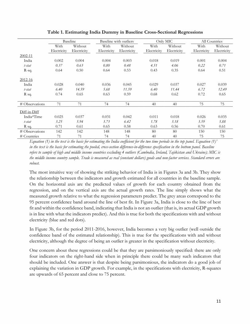
Our main results are shown in Table 1. The specification in equation (1) is estimated for the baseline

sample, comprising high income and middle income countries. We treat this as the baseline because

we want to focus on a group where statistical quality is relatively good so that India can be compared

to similar countries. Since we have the maximum data until 2016, the second period in our regressions

goes from 2012 to 2016.

In all the specifications shown in Table 1, the India dummy is statistically insignificant for the 2002-

2011 period and significant at the 1 percent confidence level for the 2012-2016 period. And in all

cases, the strict difference-in-difference dummy (bottom panel of Table 1) is significant at the 1

percent confidence level (we will return to these coefficients in the discussion of magnitudes below).

We show all the specifications with and without electricity consumption. There has been conscious

government policy to achieve 100 percent electrification started by the UPA government and

vigorously pursued by the previous BJP government. Such policy-induced electricity catch-up makes

electricity a less reliable indicator of GDP growth. As a result, the inclusion of electricity loads the

results against finding India to be an outlier in the second period. Despite this bias, India turns out to

be a consistent outlier.

Columns 1 and 2 are for the baseline sample, excluding four outliers (Cambodia, Tajikistan, Ireland

and Ukraine). In columns 3 and 4 we retain the outliers and the results remain unchanged. We then

estimate it for the sample of just middle income countries (columns 5 and 6) and for all countries

(including low income countries) in columns 7 and 8.

11

Table 1. Estimating India Dummy in Baseline Cross-Sectional Regressions

Baseline Baseline with outliers Only MIC All Countries

With

Electricity Without

Electricity With

Electricity Without

Electricity With

Electricity Without

Electricity With

Electricity Without

Electricity

2002-11

India 0.002 0.004 0.004 0.003 0.018 0.019 0.001 0.004

t-stat 0.37 0.63 0.80 0.48 4.51 4.06 0.22 0.71

R-sq. 0.64 0.50 0.64 0.53 0.43 0.35 0.64 0.51

2012-16

India 0.028 0.040 0.036 0.045 0.029 0.037 0.027 0.039

t-stat 6.40 14.59 5.68 11.59 6.40 11.44 6.72 12.49

R sq. 0.74 0.65 0.63 0.59 0.68 0.62 0.72 0.65

# Observations 71 71 74 74 40 40 75 75

Diff-in-Diff

India*Time 0.025 0.037 0.031 0.042 0.011 0.018 0.026 0.035

t-stat 3.25 5.94 3.73 6.42 1.78 3.18 3.59 5.88

R sq. 0.71 0.61 0.65 0.58 0.63 0.56 0.70 0.61

# Observations 142 142 148 148 80 80 150 150

# Countries 71 71 74 74 40 40 75 75

Equation (1) in the text is the basis for estimating the India coefficient for the two time periods in the top panel. Equation (1)’

in the text is the basis for estimating the pooled, cross-section difference-in-difference specification in the bottom panel. Baseline

refers to sample of high and middle income countries excluding 4 outliers (Cambodia, Ireland, Tajikistan and Ukraine); MIC is

the middle income country sample. Trade is measured as real (constant dollars) goods and non-factor services. Standard errors are

robust.

The most intuitive way of showing the striking behavior of India is in Figures 3a and 3b. They show

the relationship between the indicators and growth estimated for all countries in the baseline sample.

On the horizontal axis are the predicted values of growth for each country obtained from the

regression, and on the vertical axis are the actual growth rates. The line simply shows what the

measured growth relative to what the regression parameters predict. The grey areas correspond to the

95 percent confidence band around the line of best fit. In Figure 3a, India is close to the line of best

fit and within the confidence band, indicating that India is not an outlier (that is, its actual GDP growth

is in line with what the indicators predict). And this is true for both the specifications with and without

electricity (blue and red dots).

In Figure 3b, for the period 2011-2016, however, India becomes a very big outlier (well outside the

confidence band of the estimated relationship). This is true for the specifications with and without

electricity, although the degree of being an outlier is greater in the specification without electricity.

One concern about these regressions could be that they are parsimoniously specified: there are only

four indicators on the right-hand side when in principle there could be many such indicators that

should be included. One answer is that despite being parsimonious, the indicators do a good job of

explaining the variation in GDP growth. For example, in the specifications with electricity, R-squares

are upwards of 65 percent and close to 75 percent.

12

Figure 3a. Baseline Cross-Sectional Regression, 2002-2011

Figure 3b. Baseline Cross-Sectional Regression, 2012-2016

Figures 3a and 3b correspond to the specification in Columns 1 and 2 of Table 1 without the India fixed effect. The horizontal-axis shows the GDP growth predicted for each country by the regression parameters. The dots show India in relation to the cross-sectional relationship, with the blue (red) dot corresponding to the regression without (with) electricity consumption. The grey areas correspond to the 95 percent confidence band.

b.Panel estimation We can complement the cross-sectional analysis with a more demanding econometric specification

using the same difference-in-difference methodology, exploiting this time the variation within India.

13

The specification we estimate then is:

𝐿𝑛 𝐺𝐷𝑃𝑖𝑡 = 𝛽0 + 𝛽1𝐿𝑛 𝐶𝑟𝑒𝑑𝑖𝑡𝑖𝑡 + 𝛽2𝐿𝑛 𝐸𝑙𝑒𝑐𝑡𝑟𝑖𝑐𝑖𝑡𝑦𝑖𝑡 + 𝛽3𝐿𝑛 𝐸𝑥𝑝𝑜𝑟𝑡𝑠𝑖𝑡 +

𝛽4𝐿𝑛 𝐼𝑚𝑝𝑜𝑟𝑡𝑠𝑖𝑡 + 𝛽5𝐿𝑛 𝐶𝑟𝑒𝑑𝑖𝑡𝑖𝑡 ∗ 𝑃𝑜𝑠𝑡 + 𝛽6𝐿𝑛 𝐸𝑙𝑒𝑐𝑡𝑟𝑖𝑐𝑖𝑡𝑦𝑖𝑡 ∗ 𝑃𝑜𝑠𝑡 + 𝛽7𝐿𝑛 𝐸𝑥𝑝𝑜𝑟𝑡𝑠𝑖𝑡 ∗

𝑃𝑜𝑠𝑡 + 𝛽8𝐿𝑛 𝐼𝑚𝑝𝑜𝑟𝑡𝑠𝑖𝑡 ∗ 𝑃𝑜𝑠𝑡 + 𝛽9 𝐼𝑛𝑑𝑖𝑎 ∗ 𝑃𝑜𝑠𝑡 + 𝜂𝑡 + 𝛾𝑖 + 𝑢𝑖𝑡 ---------(2)

where Post takes on a value = 1 for years 2011-2016 and 0 otherwise.

Here the unit of observation is annual: to reduce the noise in annual data and also as a cross-check to

the growth specifications in the cross-section we measure all the variables in log levels. Post is the

treatment period after 2011 so that the value of Post is zero in the pre-2011 period and 1 in the post-

2011 period. Note that in this specification, we allow the relationship between the indicators and

growth to be different in the post-2011 period (captured in the interaction between each of the

indicators and the Post variable).

Our coefficient of interest is 𝛽9 which captures whether India’s level of GDP is overstated

differentially in the post-2011 period. Since GDP is measured in logs, the level over-estimation is given

by exp (𝛽9) − 1. As before, we run this specification for all the samples.

A more general version which is going to be the baseline panel specification is to augment equation

2 by adding country-specific dummies for the 2 financial crisis years because measurement in those

years would have been thrown off kilter by the extreme movements in the indicators on the right

hand side, especially trade:

𝐿𝑛 𝐺𝐷𝑃𝑖𝑡 = 𝛽0 + 𝛽1𝐿𝑛 𝐶𝑟𝑒𝑑𝑖𝑡𝑖𝑡 + 𝛽2𝐿𝑛 𝐸𝑙𝑒𝑐𝑡𝑟𝑖𝑐𝑖𝑡𝑦𝑖𝑡 + 𝛽3𝐿𝑛 𝐸𝑥𝑝𝑜𝑟𝑡𝑠𝑖𝑡 +

𝛽4𝐿𝑛 𝐼𝑚𝑝𝑜𝑟𝑡𝑠𝑖𝑡 + 𝛽5𝐿𝑛 𝐶𝑟𝑒𝑑𝑖𝑡𝑖𝑡 ∗ 𝑃𝑜𝑠𝑡 + 𝛽6𝐿𝑛 𝐸𝑙𝑒𝑐𝑡𝑟𝑖𝑐𝑖𝑡𝑦𝑖𝑡 ∗ 𝑃𝑜𝑠𝑡 + 𝛽7𝐿𝑛 𝐸𝑥𝑝𝑜𝑟𝑡𝑠𝑖𝑡 ∗

𝑃𝑜𝑠𝑡 + 𝛽8𝐿𝑛 𝐼𝑚𝑝𝑜𝑟𝑡𝑠𝑖𝑡 ∗ 𝑃𝑜𝑠𝑡 + 𝛽9 𝐼𝑛𝑑𝑖𝑎 ∗ 𝑃𝑜𝑠𝑡 + ∑ 𝛿𝑗𝑛−1𝑗=1 𝛾𝑖 ∗ 2008 + ∑ 𝜃𝑗

𝑛−1𝑗=1 𝛾𝑖 ∗

2009 + 𝜂𝑡 + 𝛾𝑖 + 𝑢𝑖𝑡 ---------(2)’

The baseline specification has 74 countries, so there are 73 dummies for each of the two financial

crisis years (2008 and 2009).10

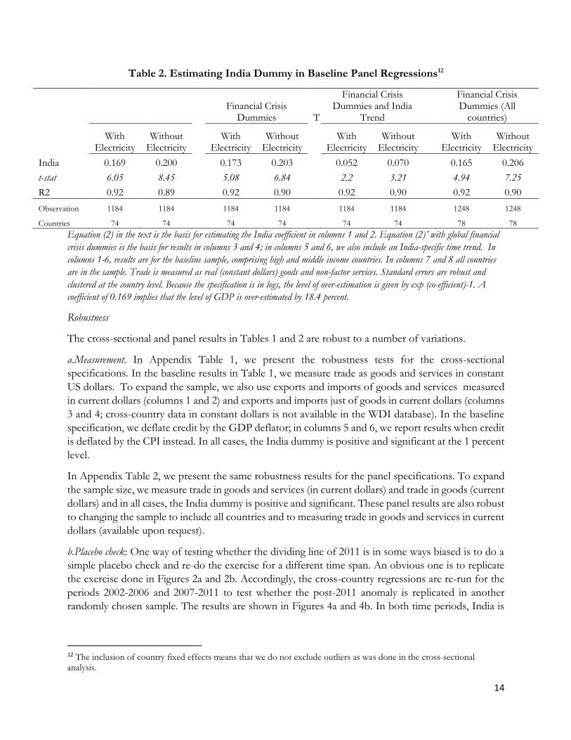
The results are displayed in Table 2. In columns 1 and 2, we estimate the treatment effect without the

financial crisis dummies; in columns 3-4 and 7-8 we add the financial crisis dummies. And in columns

5 and 6, we add in addition an India-specific time trend. In all cases, we find the India*post interaction

dummy—measuring the differential mis-estimation of the level of GDP—to be positive and

statistically significant at the 99 percent confidence interval.11

10 The pattern of sharp decline in 2008 and sharp recovery in 2009 suggests that mismeasurement could be very different

in the 2 crisis years and hence separate dummies for the two years. 11 As part of the base revisions, the level of GDP was increased in 2011-12. We account for this by splicing the level series backwards from 2011-12 so that both growth and level series are consistent.

14

Table 2. Estimating India Dummy in Baseline Panel Regressions12

Financial Crisis

Dummies T

Financial Crisis Dummies and India

Trend

Financial Crisis Dummies (All

countries)

With

Electricity Without

Electricity With

Electricity Without

Electricity With

Electricity Without

Electricity

With

Electricity Without

Electricity

India 0.169 0.200 0.173 0.203 0.052 0.070 0.165 0.206

t-stat 6.05 8.45 5.08 6.84 2.2 3.21 4.94 7.25

R2 0.92 0.89 0.92 0.90 0.92 0.90 0.92 0.90

Observation 1184 1184 1184 1184 1184 1184

1248 1248

Countries 74 74 74 74 74 74

78 78

Equation (2) in the text is the basis for estimating the India coefficient in columns 1 and 2. Equation (2)’ with global financial

crisis dummies is the basis for results in columns 3 and 4; in columns 5 and 6, we also include an India-specific time trend. In

columns 1-6, results are for the baseline sample, comprising high and middle income countries. In columns 7 and 8 all countries

are in the sample. Trade is measured as real (constant dollars) goods and non-factor services. Standard errors are robust and

clustered at the country level. Because the specification is in logs, the level of over-estimation is given by exp (co-efficient)-1. A

coefficient of 0.169 implies that the level of GDP is over-estimated by 18.4 percent.

Robustness

The cross-sectional and panel results in Tables 1 and 2 are robust to a number of variations.

a.Measurement. In Appendix Table 1, we present the robustness tests for the cross-sectional

specifications. In the baseline results in Table 1, we measure trade as goods and services in constant

US dollars. To expand the sample, we also use exports and imports of goods and services measured

in current dollars (columns 1 and 2) and exports and imports just of goods in current dollars (columns

3 and 4; cross-country data in constant dollars is not available in the WDI database). In the baseline

specification, we deflate credit by the GDP deflator; in columns 5 and 6, we report results when credit

is deflated by the CPI instead. In all cases, the India dummy is positive and significant at the 1 percent

level.

In Appendix Table 2, we present the same robustness results for the panel specifications. To expand

the sample size, we measure trade in goods and services (in current dollars) and trade in goods (current

dollars) and in all cases, the India dummy is positive and significant. These panel results are also robust

to changing the sample to include all countries and to measuring trade in goods and services in current

dollars (available upon request).

b.Placebo check: One way of testing whether the dividing line of 2011 is in some ways biased is to do a

simple placebo check and re-do the exercise for a different time span. An obvious one is to replicate

the exercise done in Figures 2a and 2b. Accordingly, the cross-country regressions are re-run for the

periods 2002-2006 and 2007-2011 to test whether the post-2011 anomaly is replicated in another

randomly chosen sample. The results are shown in Figures 4a and 4b. In both time periods, India is

12 The inclusion of country fixed effects means that we do not exclude outliers as was done in the cross-sectional analysis.

15

not an outlier (the India data point is within the confidence band), suggesting that measured GDP

growth is consistent with that in the other indicators.

Figure 4a. Placebo Check. Cross-Sectional Regression, 2002-2006

Figure 4b. Placebo Check. Cross-Sectional Regression, 2007-2011

Figures 4a and 4b are identical to Figures 2a and 2b, with the only difference that they are estimated for different time periods:

2002-2006 and 2007-2011. They correspond to the baseline regression specification with electricity included as an explanatory

variable.

16

c. Smell test: One smell test for these cross-sectional regressions is to see which other countries show

up as outliers in the cross-sectional regressions. Figures 5a and 5b show the results for baseline sample

(but with the trade variable confined to goods and measured in current dollars).13

Two prominent outliers are Ireland and China (there are others too) but the difference with India is

that their GDP growth is over-estimated in both time periods and by more than in the case of India.

These seem plausible. Allegations of GDP growth over-estimation have dogged the Chinese economy

in part because provinces have had an incentive to over-estimate GDP growth (Chen. et. al. 2019). In

the case of Ireland, the serious problem relates to the artificial booking of profits to that jurisdiction

especially by US companies (Torslov, Wier and Zucman, 2018) that leads to potential GDP over-

measurement as well.

Figure 5a: Cross-Sectional Regression, “Smell Test,” 2002-2011

13 This choice of the trade variable is forced by the non-availability of data for real goods and services for China in the

WDI database.

17

Figure 5b: Cross-Sectional Regression, “Smell Test,” 2012-2016

IV. Magnitude of GDP Growth Over-estimation

What do all these results mean for the magnitudes of over-estimation of GDP growth?

We have done the statistical analysis in many ways, with the main results displayed in Tables 1 and 2

(and the Appendix Tables). All the results robustly and consistently point to over-estimation of

GDP growth in the cross-sectional analysis and over-estimation of the level of GDP in the panel

analysis. But there is some variation in the magnitudes.

In the cross-section, in the baseline estimations (Table 1, columns 1 and 2), the magnitude of the

growth over-estimation measured in strict difference in difference terms varies from 2.5 percentage

points per year (without electricity) to 3.7 percentage points per year (with electricity) as shown in

the bottom panel.

In the panel estimation, the level of GDP is over-estimated on average by between 17 and 20

percentage points (Table 2, columns 3 and 4).

Over a 5-year period (2012-2016), an annual average growth over-estimation of 2.5 percent

translates into a cumulative level over-estimation of 15 percent and hence an average level over-

estimation of about 7-8 percent which is lower than the implied growth over-estimation from the

baseline panel specification.

It is difficult to be too precise beyond a point, but a plausible and conservative estimate that would

be consistent with the panel and cross-sectional estimates would be a growth over-estimation

between 2011 and 2016 of about 2 ½ percent per year. These are of course subject to statistical

error. The standard errors in the cross-section and panel are tightly estimated. The central estimate

of 2 ½ percent comes with a 95 percent confidence band of about 1 percent. So, instead of the

18

reported headline growth of about 7 percent between 2011 and 2016, the results in this paper

suggest a range for actual growth of between 3 ½ and 5 ½ percent.

There is one final cross-check we can do on the likely magnitudes of over-estimation. Recall that

annual average growth of imports of goods and services was 15.7 percent between 2001 and 2011.

Between 2011 and 2018, this declined dramatically to 2.5 percent despite the real effective exchange

rate having appreciated mildly over this period which should have increased import growth. GDP

growth between these two periods declined by only 0.6 percentage points.

Now, to see how unusual this is, consider that this implies a crude import elasticity of demand of 22

(13.2/0.6)! Normal estimates of this long run elasticity tend to be around 1. Even allowing for big

secular changes in the import-intensity of growth and other one-off factors, such sharp declines in

import growth are probably only consistent with large declines of annual real GDP growth. They are

more than consistent with the relatively modest declines of real GDP growth of about 2 ½ percent

which is what our central over-estimation estimates suggest; consistent because this still implies an

exceptionally high import elasticity of demand of about 4 ½.

V. In Search of Causes: Methodology plus Circumstance

Having suggested that there could have been some substantial over-estimation of GDP growth after

2011, we now turn to possible causes.

Potential Cause 1: Moving from volume to value-based estimates in manufacturing One of the key methodological changes was the move from establishment-based data from the Annual Survey of Industries (ASI) and Index of Industrial Production (IIP) to financial accounts-based data compiled by the Ministry of Corporate Affairs (MCA). This move was desirable because it apparently enlarged the scope of economic activity that was covered: more than 600,000 companies file MCA data, which could be used for NIA estimates. This move was also desirable in replacing predominantly volume-based estimates of gross value added (GVA) to value-based estimates that in principle better capture the quality and technology changes of a modern, dynamic economy. There were always doubts about the quality of some of the MCA data relating to shell companies

especially in the services sector, as the recent report by Pramit Bhattacharya (2019) highlighted. But

it is also not obvious whether these problems necessarily affect the GDP estimates. This is because

the quarterly growth estimates and their first (two) revisions are based on a much smaller set

(roughly in the range of 3000-5000) of relatively large companies. And it is not clear that the shell

company problem relates to these more critical companies. Moreover, more analysis is necessary to

see if the MCA data issues affect estimation of GDP levels or growth rates and whether it is nominal

and/or real estimates that are impacted.

But the move to financial accounts combined with a change in the external environment during the

post-2011 period might still have had significant consequences. In particular, oil prices declined

substantially. Under the old, establishment-based GDP estimates, price changes mattered less

because real growth numbers were largely based on volumes not values. Under the new system,

however, values had to be deflated by prices to get real magnitudes. And this mattered crucially for

19

the manufacturing sector where the often-dramatic changes in oil prices can heavily influence input

costs (See also Dholakia, Nagraj and Pandya, 2018).

Ideally, if output values are deflated by output prices and input values by input prices (what is called

“double deflation”), real value added can be properly estimated. But the methodology did not also

involve a move to such double deflation; the methodology involved deflating both output and input

values by output prices.14 This immediately induces a bias as the example below shows.

The example compares real growth rates of value added in three scenarios: volume extrapolation (as

under the old system), value estimation combined with double deflation, and value estimation

combined with single (output price) deflation. In the top panel input and output quantities and prices

are assumed. To keep it simple, the only variable that changes in the second period is a decline in input

prices from Rs. 10 to Rs. 5. In this example, true real growth is zero because input and output

quantities do not change by construction.

Under double deflation, growth is zero percent because input cost changes are deflated away by lower

input prices so that real input costs and hence real value added remain unchanged. But under single

deflation, lower nominal input values are taken as a sign that real inputs have declined (because the

deflator used is the output price, which doesn’t change), thereby increasing real value added. In the

example, real value-added growth in period 2 under single deflation is 21 percent.

Table 3: Impact of Changes in Relative Prices of Outputs and Inputs on Real Value Added

Measurement: An Illustrative Example

In other words, the inappropriate use of single deflation can artificially inflate growth figures by

significant amounts when oil prices fall sharply, as they did in the post-2011 period, especially the

post-2014 period, as Figure 6 shows.

If this analysis is correct, it has three testable propositions. First, formal manufacturing value added,

which is particularly oil-intensive, should be significantly affected in the post-2011 period. Second,

manufacturing value added growth should be over-estimated post-2011. Third, manufacturing value

added should be more sensitive to the output-input price wedge post-2011 than pre-2011 because in

the earlier period estimation was more volume based.

14 The impact of not using double deflation will not only vary over time but also across countries, depending on whether they are net exporters or importers and the magnitude of their oil dependence.

20

We find evidence in favour of all three propositions. And a rough calculation suggests that the mis-

estimation of formal manufacturing can itself explain about 1 percentage point of the overall GDP

growth over-estimation of 2 ½ percentage points.

Figure 6. Oil Price (Brent; $/barrel), 2009-2018

Proposition 1. Formal manufacturing value-added significantly affected. Two independent sources are

available for measuring the performance of the formal manufacturing sector on a quarterly basis: the

IIP (Manufacturing) and manufacturing exports.

The NIA estimates real GVA growth for the formal manufacturing sector using company data and

proxies informal sector manufacturing growth using the IIP even though the latter is (a) based on a

sample of formal sector establishments and (b) is mostly a volume metric. In principle, the volume and

value added metrics should not diverge unless the technological efficiency of the economy—defined

as the relationship between intermediate inputs and output—changes (efficiency includes

improvements in product quality). If an economy becomes more efficient at using inputs, then volume

indicators will underestimate true value-added growth. A corollary—and a source of deep confusion—

is that if prices of outputs or intermediates change without any change in the technological efficiency,

volume growth and real GVA growth should not diverge. The fact that manufacturing companies

make more profit because, say, oil prices decline should not alter the relationship between volume and

value-added estimates, and does not signify higher real value added even though nominal value added

may have increased.

That manufacturing value added is particularly distorted in the second period is revealed in Figure 1

above. Pre-2011, the correlation between formal manufacturing value added growth and IIP

manufacturing growth, which are both measuring the same scope of real activity (formal

manufacturing), is high and positive (0.7); post-2011, it turns negative (-0.1). This is bizarre.15

15 Similarly, the correlation between manufacturing value added and real credit growth to industry drops from 0.47

before 2011 to 0.15 after.

21

Another measure of the distortion is suggested by comparing the correlation between real GVA

growth and growth in manufacturing exports (in dollars). Normally, higher manufacturing growth

should be associated with higher growth in manufacturing exports. Since manufacturing production

precedes manufacturing exports, we look at the correlation between manufacturing and exports a

quarter later. During Q3 2008-09 to Q4 2012-13 (old series), this correlation was expectedly positive

at 0.4. But for the period covered by the new GVA series, this correlation becomes negative at -0.3,

which is very unusual (Figures 7a and 7b below). So, again, the old real GVA growth series yields

reasonably plausible relationships with other related series, but the new series yields counter-intuitive

results.

Figure 7: Growth of formal manufacturing sector GVA and manufacturing exports (in %,

exports are for one-quarter ahead)16

7a. Pre-2011

16 Manufacturing exports cover HS chapters 28-96. Manufacturing exports are in current dollars.

09Q1

09Q2

09Q3

09Q4

10Q1

10Q2

10Q3

10Q4

11Q1

11Q211Q3

11Q4 12Q1

12Q2

12Q312Q4

-30%

-20%

-10%

0%

10%

20%

30%

40%

50%

60%

70%

-5% 0% 5% 10% 15% 20% 25% 30%

Man

ufa

cturi

ng

Exp

ort

s G

row

th

Real GVA Formal Manufacturing Growth

Correlation = 0.4

22

7b. Post-2011

The old series begins in 2009 Q1 because that is when disaggregated quarterly data for manufacturing exports becomes available. New series

spans the period 2012-13 to second quarter of 2018-19.

Proposition 2. Formal manufacturing value-added growth over-estimated: Figure 8 below plots the

wedge between quarterly real GVA growth for the two measures of formal manufacturing sector,

from the NIA and manufacturing volume growth from the IIP, from 2001 to 2017.

Pre-2011, the relationship was as one might expect. Real GVA growth in the formal manufacturing

sector and IIP manufacturing growth diverged but in both directions so that the average difference

was just 0.9 percentage points (going back to 2005) or 0.5 percentage points (going back to 2001).

However, post-2011, under the new series, the divergence is almost entirely one way, with real GVA

growth consistently exceeding IIP growth by about 5.9 percentage points on average. Under the new

series, formal manufacturing real GVA has grown by 9.5 percent per annum between 2011-12 Q1 and

2018-19 Q3. For the same period average IIP growth has been 3.6 percent.

With reasonable quality and efficiency growth, the GVA number should probably exceed the IIP

number and the excess in the first period of 0.9 percentage points seems reasonable. But the sudden

jump to 5.9 percentage points in the post-2011 period seems baffling.

In fact, if we assumed that the relationship between IIP manufacturing and GVA manufacturing

should have been similar before and after 2011, we can crudely say that the latter should have been

about 4.6 percent (3.6 percent IIP manufacturing growth plus 1 percent for technical improvements

suggested by the pre-2011 estimates) instead of 9.5 percent. This difference when multiplied by the

share of manufacturing in GVA (about 17 percent) yields an over-estimation of nearly 0.9

percentage points, roughly one-third of the over-estimation of total GDP growth.

13Q1

13Q2

13Q3

13Q4

14Q1

14Q2

14Q3

14Q4

15Q1

15Q2

15Q3 15Q4

16Q1

16Q2

16Q3

16Q417Q1

17Q2

17Q3

17Q418Q1 18Q2

18Q3

18Q4 19Q1

-15%

-10%

-5%

0%

5%

10%

15%

20%

-5% 0% 5% 10% 15% 20% 25%

Rea

l G

VA

Fo

rmal

Man

ufa

cturi

ng

Gro

wth

Manufacturing Exports Growth

Correlation = -

23

Figure 8. Wedge Between Real Formal Manufacturing Growth in GVA and IIP (percentage

points)

Proposition 3. Over-estimation of formal manufacturing related to output-input price wedge: The

final piece of evidence relates to the relationship between the divergence and the output-input price

wedge. Output prices are proxied by the CPI, and input prices by the WPI, because the WPI is heavily

weighted toward commodities, which are typically used as inputs.

Figure 9 plots the CPI-WPI wedge and the GVA-IIP wedge for both the old (top) and new series

(bottom). Under the old series, the correlation was not high indicating that real GVA measurements

were less susceptible to price changes, as they should be.17 But under the new series, the correlation

increases to 0.62 and the wedge becomes more vulnerable to relative price changes. In effect, the

lower the WPI inflation (proxying the cost of inputs) relative to CPI inflation, the more GVA growth

is relative to IIP growth. And this positive correlation (0.6) is exactly what Figure 9 shows for the new

series.

17 Another possible explanation for the IIP-GVA wedge in manufacturing is the differences in the sample of companies

being tracked under IIP and the MCA quarterly filings. But when the revised IIP, rebased to 2011-12, was introduced, the

sample covered more than 80 percent of the formal industrial sector and hence the wedge attributable to this difference

should now be minor. In addition, the difference between the establishment-focussed approach followed in the IIP and

the company-focussed approach followed in the company data can also explain part of the IIP-GVA wedge, but only a

small part.

-15

-12

-9

-6

-3

0

3

6

9

12

15

18

2000-0

1

2001-0

2

2002-0

3

2003-0

4

2004-0

5

2005-0

6

2006-0

7

2007-0

8

2008-0

9

2009-1

0

2010-1

1

2011-1

2

2012-1

3

2013-1

4

2014-1

5

2015-1

6

2016-1

7

2017-1

8

2018-1

9

Old Methodology (average wedge: 0.5 percentage points)

New Methodology (average wedge: 5.9 percentage points)

24

Figure 9: Correlation between: (a) wedge between formal manufacturing growth and

manufacturing growth from IIP, and, (b) wedge between CPI and WPI

9a. Pre-2011

9b. Post-2011

The old series spans the period 2006-07 Q4 to 2011-12 Q4 and does not extend back because consistent price data are not

available. The new series spans the period 2013-14Q4 to 2018-19 Q4; it therefore excludes seven quarters of data because for

that period (2012-13Q1-2013-14Q3) CPI and WPI data are not in the same base.

Potential Cause 2: Deflating Services by Manufacturing Deflators

The Mid-Year Economic Analysis of December 2015 discussed the deflators used in converting

nominal value estimates in services to real estimates. In particular, while consumer services values

07Q4

08Q1

08Q208Q3

08Q4

09Q109Q2

09Q3 09Q4

10Q110Q210Q3

10Q4

11Q111Q211Q311Q4

12Q1 12Q2

12Q3 12Q4

-12

-10

-8

-6

-4

-2

0

2

4

6

8

10

-4 -2 0 2 4 6 8 10 12

GV

A-I

IP (

Mfg

.) W

edge

CPI-WPI (Inflation) Wedge

Correlation = 0.36

14Q1

14Q2

14Q3

14Q4

15Q115Q2

15Q3

15Q4

16Q116Q2

16Q3

16Q4

17Q117Q2

17Q317Q4

18Q1

18Q2

18Q318Q4

19Q1

19Q219Q3

-6

-4

-2

0

2

4

6

8

10

12

14

-4 -2 0 2 4 6 8 10 12

GV

A-I

IP(M

fg) W

edge

CPI-WPI (Inflation) Wedge

Correlation = 0.6

25

are deflated by the relevant CPI-services index, producer services (including trade and repair;

storage; information and computer-related; professional, scientific and technical activities, including

R & D; real estate), which account for about 20 percent of overall GVA are deflated by the

aggregate WPI manufacturing index.

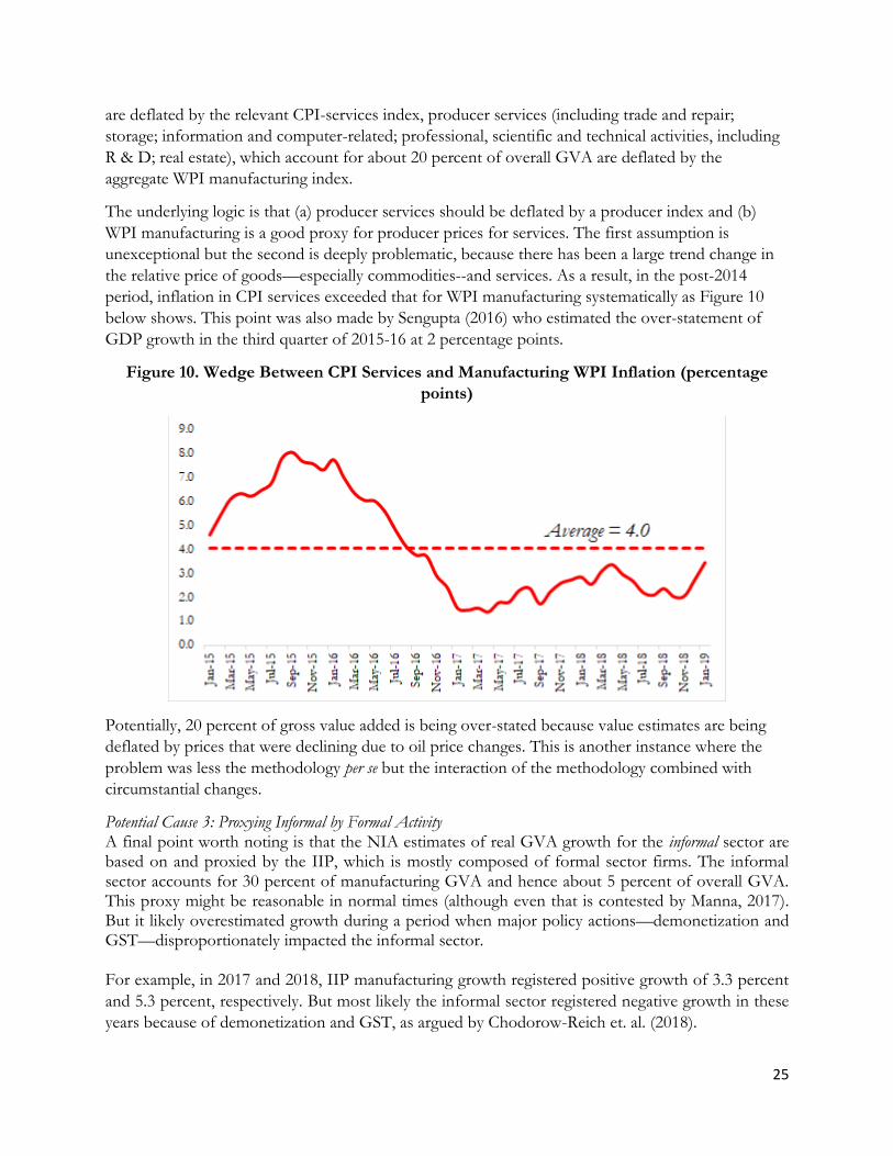
The underlying logic is that (a) producer services should be deflated by a producer index and (b)

WPI manufacturing is a good proxy for producer prices for services. The first assumption is

unexceptional but the second is deeply problematic, because there has been a large trend change in

the relative price of goods—especially commodities--and services. As a result, in the post-2014

period, inflation in CPI services exceeded that for WPI manufacturing systematically as Figure 10

below shows. This point was also made by Sengupta (2016) who estimated the over-statement of

GDP growth in the third quarter of 2015-16 at 2 percentage points.

Figure 10. Wedge Between CPI Services and Manufacturing WPI Inflation (percentage

points)

Potentially, 20 percent of gross value added is being over-stated because value estimates are being

deflated by prices that were declining due to oil price changes. This is another instance where the

problem was less the methodology per se but the interaction of the methodology combined with

circumstantial changes.

Potential Cause 3: Proxying Informal by Formal Activity A final point worth noting is that the NIA estimates of real GVA growth for the informal sector are based on and proxied by the IIP, which is mostly composed of formal sector firms. The informal sector accounts for 30 percent of manufacturing GVA and hence about 5 percent of overall GVA. This proxy might be reasonable in normal times (although even that is contested by Manna, 2017). But it likely overestimated growth during a period when major policy actions—demonetization and GST—disproportionately impacted the informal sector. For example, in 2017 and 2018, IIP manufacturing growth registered positive growth of 3.3 percent

and 5.3 percent, respectively. But most likely the informal sector registered negative growth in these

years because of demonetization and GST, as argued by Chodorow-Reich et. al. (2018).

26

This, however, is not an explanation for our results because our baseline results do not cover the

period beyond March 2017 when the impacts of demonetization, and especially the GST, would have

been most severe.

VI. Issues for Further Research

This paper should be seen as the beginning of a research agenda focusing on India’s National

Income Accounts estimates. A number of issues still need to be addressed. For example, this paper

has focused only on the real GDP estimates. One natural question is whether, similar problems

afflict the measurement of nominal GDP growth. Future work should investigate this.

If nominal GDP growth is also over-estimated, then of course it has other implications. For

example, it would mean that India’s tax performance (including the new GST) has been more

impressive than currently believed. On the other hand, it would also mean that many important

fiscal ratios (deficit/GDP and debt/GDP) are worse than currently believed, because the

denominator in these ratios is nominal GDP, which could be lower than currently measured. It

would also mean that the decline in financial savings that has caused much alarm is smaller than

feared. Another implication would be that the source of the mismeasurement cannot just relate to

the measurement of price deflators.

On the other hand, if only real GDP growth were mismeasured, it would have other implications. It

would imply that the mismeasurement of real GDP is largely related to mismeasurement of price

deflators, which are higher than currently believed.

If, in fact the mismeasurement stems from deflator issues which in turn stems from the particular

configuration of output and input prices, then should we not see mismeasurement in the other

direction: in particular, when oil prices rise as in 2018, should we not see an under-estimation of

GDP growth? In this paper, the data in Figures 1 and 2 extend through 2018 but the data in the

regression analysis extend only through 2016.

Another unresolved issue relates to the adding-up constraint. If GVA is over-estimated from the

production side, what is the counterpart over-estimation on the expenditure side – consumption,

investment, or both?

VII. Conclusions

A variety of evidence suggests that the methodology changes introduced for the post-2011 GDP

estimates led to an over-estimation of GDP growth. Given the nature of the data, and the

impossibility for researchers to reproduce the detailed methodology underlying the GDP estimates,

the results in the paper are by no means the final word. Further research, building on the results in

the paper—which itself builds on preliminary work done in the Economic Survey—will surely uncover

further insights. Accordingly, the data and codes underlying this paper will soon be made public for

scrutiny and further analysis.

That said, the evidence is too broad and robust, the anomalies and puzzles too numerous, the

magnitudes of over-estimation too large, and the stakes for the economy and country too high for

this evidence not to be debated seriously.

27

Growth over-estimates matter not just for reputational reasons but critically for internal policy-

making. If the new evidence is right, it would imply that both monetary and fiscal policies over the

last years were overly tight from a cyclical perspective. Consider this. Real policy interest rates in the

last few years have been at about 2.5 percent, well above the RBI’s own estimate of the neutral rate

of about 1.25-1.5 percent. Now, if real activity is weak, the policy rate should be below the neutral

rate instead of exceeding it: the net difference could have been rates about 150 basis points higher

than necessary. The Indian policy automobile has been navigated with a faulty or even broken

speedometer.

In addition, if statistics are potentially misleading about the overall health of the economy, they

influence the impetus for reform in serious and perverse ways. For example, if India’s GDP growth

had been appropriately measured, the urgency to act on the banking system challenges or agriculture

or unemployment could have been very different. It is understandable when policy makers favour

the status quo if that status quo is apparently delivering the fastest growth rate of any major

economy in the world. But if growth is actually 4.5 percent instead of 7 percent, attitudes to policy

action should and would be very different.

These findings have two major policy implications going forward.

First, growth must be restored as a key policy objective. Policy discourse in India in recent years has

focused on employment, agriculture and redistribution more broadly. It has also sought to explain

the apparent puzzles of ongoing and intensifying corporate and financial system stress, weak new

project announcements, and persistently low capacity utilization in manufacturing. In all these cases,

there has been a sense that all of these weakness were anomalies, existing despite good growth,

captured in the popular narrative of “jobless growth.” In reality, all these weaknesses may have

partly stemmed from weaker-than-believed growth. Going forward, there must be both the urgency

from the new knowledge that growth is weaker-than-believed and the re-embrace of growth as

necessary to accomplish other objectives.

Second, the quality and integrity of data needs to be improved. The methodological changes begun

in 2012 and were completed in 2014, affecting growth numbers for both the Congress- and BJP-led

governments. Accordingly, the statisticians and technocrats who were involved in making the

methodology changes need to reflect on the implications of this evidence.

India must restore the reputational damage suffered to data generation in India across the board—

from GDP to employment to government accounts—not just by conferring statutory independence

on the National Statistical Commission, but also appointing people with stellar technical and

personal reputations. At the same time, the entire methodology and implementation for GDP

estimation must be revisited by an independent task force, comprising both national and

international experts, with impeccable technical credentials and demonstrable stature. And it must

include not just statisticians but also macro-economists and policy practitioners. Indeed, the

revisiting of NIA estimation will throw up exciting, new opportunities, for example using the large

amounts of transactions-level GST data to estimate—for the first time in India—expenditure-based

estimates of GDP.

28

If statistics are sacred enough to require insulation from political pressures, they are perhaps also too

important to be left to the statisticians alone. Nothing less than the future of the Indian economy

and the lives of 1.4 billion citizens rides on getting numbers and measurement right.

As we measure, so India will go.

29

References

Bhattacharya, Pramit, 2019, “New GDP series faces fresh questions after NSSO discovers holes, “

(https://www.livemint.com/news/india/new-gdp-series-faces-fresh-questions-after-nsso-discovers-

holes-1557250830351.html).

Chen, Wei, Xilu Chen, Chang-Tai Hsieh, Zheng (Michael) Song, 2019, “A Forensic Examination of

China’s National Accounts,” Brookings Papers on Economic Activity, March 7–8, 2019Chodorow-Reich,

Dholakia, Ravindra, 2015, “Double Deflation Method and Growth of Manufacturing,” Economic and

Political Weekly, Vol. 50, Issue No. 41, 10.

Dholakia, Ravindra, R. Nagaraj, and Manish Pandya, 2018, “Manufacturing Output in New GDP

Series,” Economic and Political Weekly, Vol. 53, Issue No. 35, 01 Sep, 2018

Chodorow-Reich, Gabriel, Gita Gopinath, Prachi Mishra, and Abhinav Narayanan 2018, “Cash and

the Economy: Evidence from India's Demonetization,” NBER Working Paper 25370.

Government of India, 2015, “Mid-Year Economic Analysis,”

https://dea.gov.in/sites/default/files/MYR201516English.pdf, pp. 6-8

Government of India, 2017, “Economic Survey, 2016-17, Volume 2”,

https://www.indiabudget.gov.in/es2016-17/echapter_vol2.pdf, pp. 27-28.

Manna, G.C., 2017, “An Investigation into some contentious issues in GDP estimation,” ISPE

Journal.

Kazmin, Amy, 2019, “Economists condemn politicization of Modi government data, Financial

Times, March 15, 2019 (https://www.ft.com/content/38b9d94c-46d4-11e9-b168-96a37d002cd3)

Nagaraj, R and T N Srinivasan, 2016, “Measuring India’s GDP Growth: Unpacking the Analytics & Data Issues behind a Controversy that Refuses to Go Away,” India Policy Forum. Sapre, Amey and Rajeshwari Sengupta, 2017, “An analysis of revisions in Indian GDP data',”

National Institute of Public Finance and Policy Working Paper, 213.

Sengupta, R, 2016, “Real GDP is growing at 5%, not 7.1%,”

https://www.livemint.com/Opinion/58qihTaOIRd3rPyf1eK09L/Real-GDP-is-growing-at-5-not-

71.html

Tørsløv, Thomas, Ludvig S. Wier and Gabriel Zucman, 2018, “The Missing profits of Nations,”

NBER Working Paper, 24701.

30

Appendix Table 1. Cross-Sectional Results, Robustness

In columns 1 and 2, the trade variable—goods and services--is measured in current dollars; in columns 3 and 4, the trade variable—goods only—is measured in current dollars; in columns 5 and 6, the nominal credit variable is deflated by the CPI instead of the GDP deflator. In all columns, the sample comprises high and middle income countries.

Appendix Table 2: Panel Regression Results, Robustness

Goods and Services Goods Only Credit Deflated by

CPI

With Electricit

y

Without Electricit

y

With Electricit

y

Without Electricit

y

With Electricit

y

Without Electricit

y

India 0.123 0.150 0.124 0.148 0.183 0.214

t-stat 2.74 3.58 2.45 3.18 5.44 7.14

R-square 0.93 0.90 0.92 0.90 0.92 0.89 Observations 1312 1312 1296 1296 1120 1120

Countries 82 82 81 81 70 70

In columns 1 and 2, the trade variable—goods and services--is measured in current dollars; in columns 3 and 4, the trade variable—goods only—is measured in current dollars; in columns 5 and 6, the credit variable is deflated by the consumer price index. In all columns, the sample comprises high and middle income countries and is based on the baseline specification in equation 2’ in the text.

31

Appendix Table 3: Details of Cross-Sectional Results in Baseline Specifications

(1) (2) (3) (4)

VARIABLES GDP Growth

2002-11

GDP Growth

2012-16

GDP Growth

2002-11

GDP Growth

2012-16

India 0.002 0.028*** 0.004 0.040***

[0.006] [0.004] [0.006] [0.003]

Credit 0.064* 0.149*** 0.054 0.250***

[0.033] [0.031] [0.034] [0.028]

Electricity 0.279*** 0.324***

[0.066] [0.084]

Import 0.207*** 0.109* 0.299*** 0.109*

[0.072] [0.055] [0.082] [0.056]

Exports -0.000 0.038 0.020 0.019

[0.065] [0.048] [0.073] [0.055]

Constant 0.010** 0.010*** 0.013*** 0.013***

[0.004] [0.003] [0.004] [0.003]

Observations 71 71 71 71

R-squared 0.638 0.741 0.496 0.655

Model OLS OLS OLS OLS

Std. Errors Robust Robust Robust Robust

Regressions correspond to the baseline specification in columns 1-4 of Table 1, respectively. Robust

standard errors in brackets; *** p<0.01, ** p<0.05, * p<0.1

32

Appendix Table 4: Details of Panel Results in Baseline Specifications

(1) (2)

VARIABLES GDP GDP

India*Post 0.173*** 0.203***

[0.034] [0.030]

Credit*Post -0.001 0.006

[0.004] [0.005]

Electricity*Post -0.017

[0.017]

Import*Post 0.081* 0.023

[0.045] [0.054]

Export*Post -0.076* -0.052

[0.039] [0.052]

Credit 0.050** 0.069***

[0.025] [0.022]

Electricity 0.251***

[0.064]

Import 0.224*** 0.297***

[0.054] [0.054]

Export 0.002 0.031

[0.043] [0.049]

Constant 8.389*** 9.642***

[0.798] [0.573]

Observations 1,184 1,184

R-squared 0.922 0.898

Number of Countries 74 74

Country-Specific Global

Financial Crisis Dummy

YES YES

Country Fixed Effects YES YES

Time Fixed Effects YES YES

Std. Errors Cluster Country level Cluster Country level

The results correspond to equation 2’ in the text and to the results in columns 3 and 4 of Table 2. Robust

standard errors in brackets; *** p<0.01, ** p<0.05, * p<0.1; Post= Post 2011; Trade is measured as export

and import of goods and services in real local currency units

33

Data Appendix

Figure Variable Source

Figures 1, 2a and 2b

Two-Wheeler, Foreign Tourist, Airline Passenger, Commercial Vehicle, Cement, Petroleum, Steel, Tractor

Center for the Monitoring of the Indian Economy (CMIE)

Domestic Credit to Private Sector (Credit), Import of Goods and Services, Export of Goods and Services

World Development Indicators (WDI, World Bank)

Credit Industry RBI

Electricity Michael Greenstone

Index of Industrial Production (IIP), Gross Value Added (GVA)

Ministry of Statistics and Program Implementation (MOSPI)

Figures 3a, 3b, 4a, and 4b

GDP Constant LCU, Export and Import of Goods and Services at Constant USD, Real Credit (Deflated by GDP Deflators)

WDI

Electricity Michael Greenstone

Figures 5a and 5b

Same as Figure 4a and 4b except for Trade Indicators. Export and Import of Goods at Current USD

WDI

Figure 6 Oil Price (Brent; USD/barrel) https://www.macrotrends.net/2480/brent-crude-oil-prices-10-year-daily-chart

Figure 7 Formal Manufacturing GVA and Manufacturing Exports

MOSPI and Ministry of Commerce and Industry

Figure 8 Formal Manufacturing GVA and IIP Manufacturing

Ministry of Statistics and Program Implementation (MOSPI)

Figures 9 and 10

Formal Manufacturing, IIP Manufacturing and Consumer Price Index (CPI)

Ministry of Statistics and Program Implementation (MOSPI)

Wholesale Price Index (WPI) Ministry of Commerce and Industry

Table Variable Source

Tables 1 and 2

GDP Constant LCU, Export and Import of Goods and Services at Constant USD, Real Credit (Deflated by GDP Deflators)

WDI

Electricity EPIC

Table 3 Illustrative Example Own Calculations