1

Increasing the structure Increasing the structure determination success ratedetermination success rate

1 Screening infrastructurea) offline targeting and unattended execution

b) Room temperature tray screening

2 Crystal triage technologya) Simulate the experiment to discover minimum

required data quality

b) Geometric strategy for unpredictable damage

2

CHL conveyor

Cryogenic sample conveyor labyrinth installed in beamline 8.3.1. Samples can be inserted into the external port of the conveyor (right) and moved into the robot-accessible internal port (left) without ever turning off the x-rays and disrupting ongoing data collection.

3

Pepper Screening

Samples that have not been pre-targeted may be subjected to “pepper screening”. Here the silouhette of the loop is taken as a collection of potential targets. First, the centroid of the silouhette is selected as a target and the pixels corresponding to the exposed area are eliminated as potential targets. Next, the new centroid is taken as the next target. This process is repeated until no pixels are left. The result is a self-avoiding series of targets that acheives maximum coverage of the loop in the least amount of shots.

4

Plate goniometers

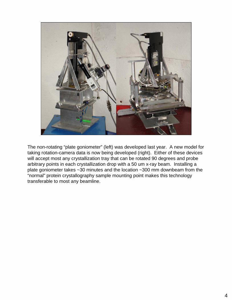
The non-rotating “plate goniometer” (left) was developed last year. A new model for taking rotation-camera data is now being developed (right). Either of these devices will accept most any crystallization tray that can be rotated 90 degrees and probe arbitrary points in each crystallization drop with a 50 um x-ray beam. Installing a plate goniometer takes ~30 minutes and the location ~300 mm downbeam from the “normal” protein crystallography sample mounting point makes this technology transferable to most any beamline.

5

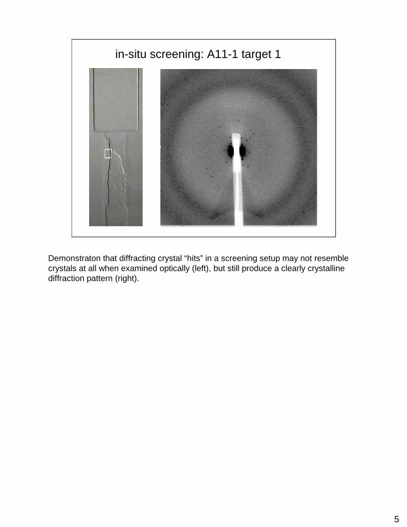
in-situ screening: A11-1 target 1

Demonstraton that diffracting crystal “hits” in a screening setup may not resemble crystals at all when examined optically (left), but still produce a clearly crystalline diffraction pattern (right).

6

realreal

Simulated diffraction imageSimulated diffraction imagesimulatedsimulated

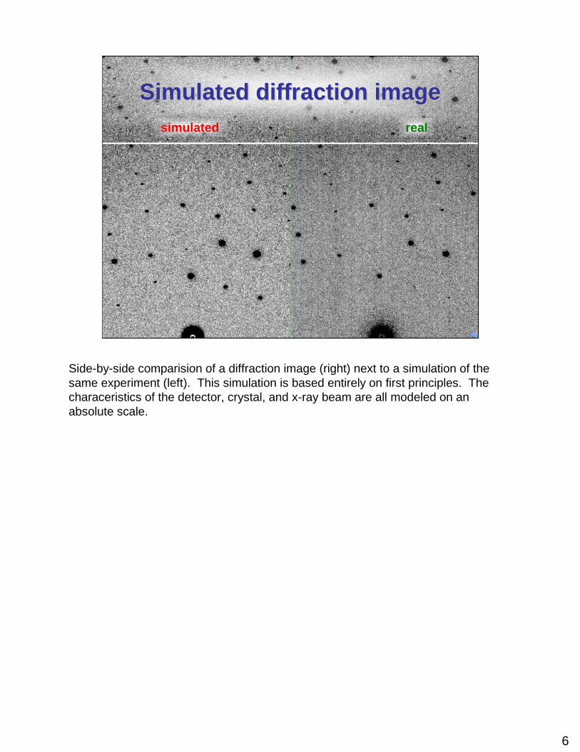
Side-by-side comparision of a diffraction image (right) next to a simulation of the same experiment (left). This simulation is based entirely on first principles. The characeristics of the detector, crystal, and x-ray beam are all modeled on an absolute scale.

7

1.6I/sd (1.4 Ǻ)1.9

0.231Rfree0.205

0.184Rcryst0.170

0.6090CC(1H87)0.6270

0.664FOMDM0.545

0.192FOM0.178

3.476mlphare f”3.871

31.46PADFPH36.8

1.0 2.2 0.065SDCORR1.7 4.0 0.020

16.2I/sd18.9

6.2%Rmerge5.4%

RealstatisticSimulated

Results of processing the images from the simulation next to the results of processing data collected from the real-world experiment that was modeled in the simulation. The simulation produces slightly better data than reality, but most of the statistics are remarkably close. SDCORR is the optimised error model derived in the program SCALA. PADFPH is the maximum phased anomalous difference Fourier peak height. FOM is the figure of merit from MLPHARE. FOMDM is the figure of merit from the program DM. CC(1H87) is the correlation coefficient of the map from DM to the published model (PDB id 1H87).

8

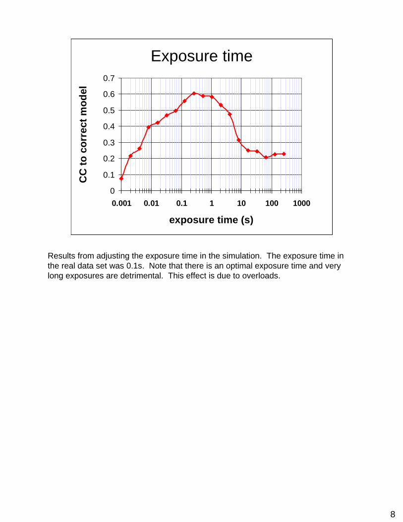
Exposure time

0

0.1

0.2

0.3

0.4

0.5

0.6

0.7

0.001 0.01 0.1 1 10 100 1000

exposure time (s)

CC

to c

orre

ct m

odel

Results from adjusting the exposure time in the simulation. The exposure time in the real data set was 0.1s. Note that there is an optimal exposure time and very long exposures are detrimental. This effect is due to overloads.

9

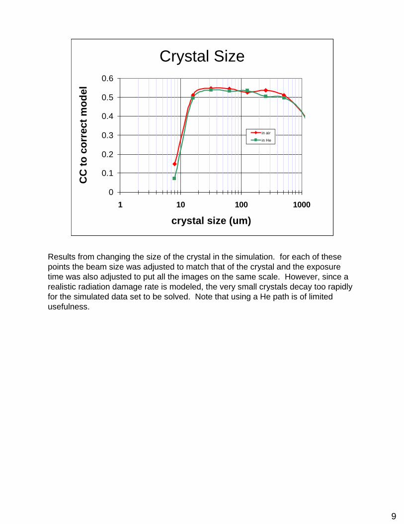
Crystal Size

0

0.1

0.2

0.3

0.4

0.5

0.6

1 10 100 1000

in air

in He

crystal size (um)

CC

to c

orre

ct m

odel

Results from changing the size of the crystal in the simulation. for each of these points the beam size was adjusted to match that of the crystal and the exposure time was also adjusted to put all the images on the same scale. However, since a realistic radiation damage rate is modeled, the very small crystals decay too rapidly for the simulated data set to be solved. Note that using a He path is of limited usefulness.

10

Shutter Jitter

0

0.1

0.2

0.3

0.4

0.5

0.6

0.7

0.8

0.9

0.01 0.1 1 10 100

rms timing error (% exposure)

CC

to c

orre

ct m

odel

Sources of noise in the beamline can be dertrimental to MAD/SAD. In this case, the Bijvoet ratio <delta-F>/<F> was 3.5%. Notice that the “crossover” point of this curve occurrs when the noise from the shutter amounts to 3.5%. Note also that shutter noise of less than 1% error has the same final structure quality as no shutter noise at all. This sigmoidal behavior is typical of these simulations and illustrates how small signals are expected to interact with noise.

11

Site Occupancy

0

0.1

0.2

0.3

0.4

0.5

0.6

0.01 0.1 1 10

Gd site occupancy

CC

to c

orre

ct m

odel

Increasing the signal strength is not always beneficial. In this simulation, using an occupancy for the Gd sites above unity simulates using a more powerful anomalous scatterer. In this case, the map correlation declines because this is a SAD experiment and the estimation of FH becomes less accurate as the FH vector becomes large. For a MAD experiment, the curve is flat at occupancy = 1 or higher.

12

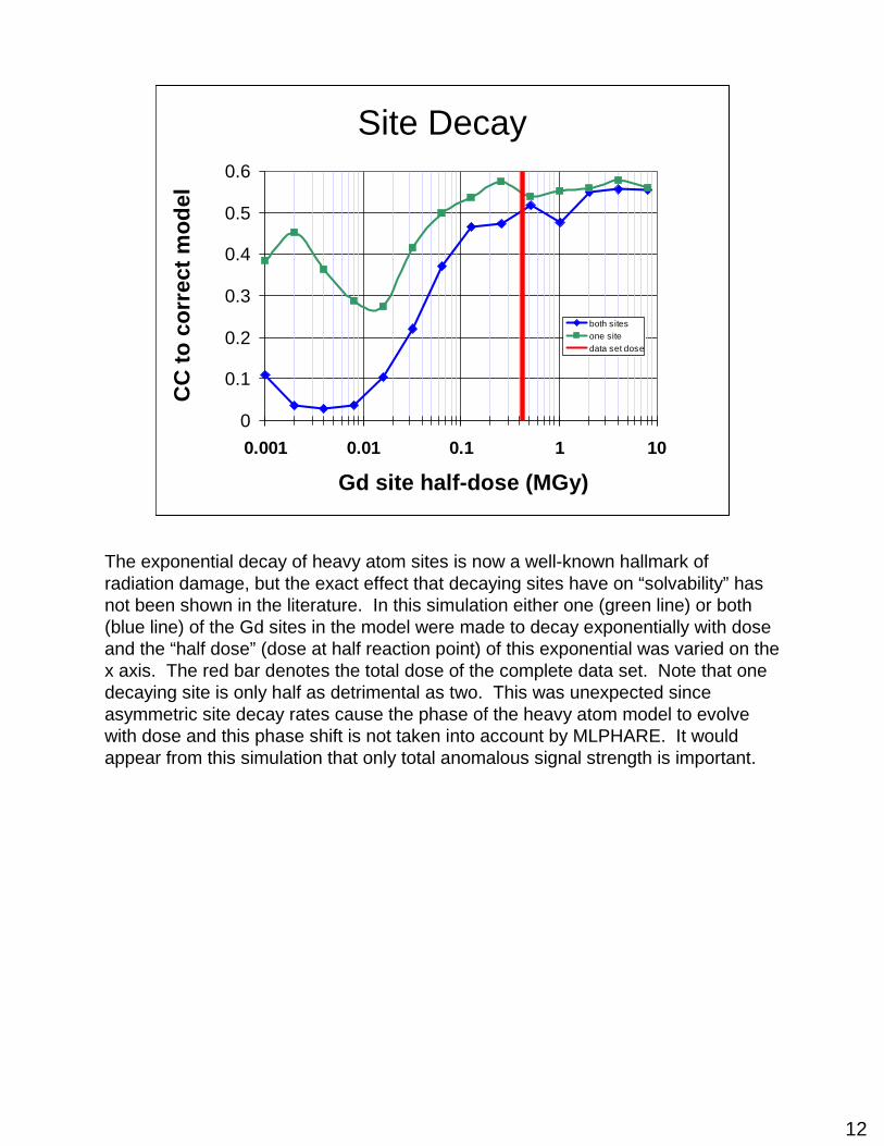
Site Decay

0

0.1

0.2

0.3

0.4

0.5

0.6

0.001 0.01 0.1 1 10

both sitesone sitedata set dose

Gd site half-dose (MGy)

CC

to c

orre

ct m

odel

The exponential decay of heavy atom sites is now a well-known hallmark of radiation damage, but the exact effect that decaying sites have on “solvability” has not been shown in the literature. In this simulation either one (green line) or both (blue line) of the Gd sites in the model were made to decay exponentially with dose and the “half dose” (dose at half reaction point) of this exponential was varied on the x axis. The red bar denotes the total dose of the complete data set. Note that one decaying site is only half as detrimental as two. This was unexpected since asymmetric site decay rates cause the phase of the heavy atom model to evolve with dose and this phase shift is not taken into account by MLPHARE. It would appear from this simulation that only total anomalous signal strength is important.

13

Detective Quantum Efficiency

0

0.1

0.2

0.3

0.4

0.5

0.6

0 0.2 0.4 0.6 0.8 1

fraction of photons “detected”

CC

to c

orre

ct m

odel

Detective quantum efficiency (DQE) is a highly prized feature of new detectors. The “DQE” varied in this simulation is the fraction of incident photons that contribute to the “counting noise” step. Fewer “detected” photons means that the signal/noise drops accordingly. Not that the simulation is highly insensitive to this DQE. The reason for this is that the DQE is highly related to exposure time (explored on an earlier slide). The “turnover point” on this graph corresponds to an effective exposure time of 0.01s, which is also the turnover point on the exposure time graph. It would appear from this simulation that a DQE close to unity is desirable, but a fractional drop in DQE from unity can be effectively compensated by increasing the exposure time by that same fraction.

14

Read-out noise

0

0.2

0.4

0.6

0.8

1

1E-1 1E+0 1E+1 1E+2 1E+3 1E+4 1E+5 1E+6

myoglobin (Fe)

lysozyme (Gd)

effective redundancy

norm

aliz

ed p

eak

heig

ht

Q315r Q315Mar325HE

0.1 1 10 100 103 104 105 106

Pilatus

Modern detector developers are endeavoring to push the contribution of intrinsic noise (read-out noise in the case of a CCD) to zero. One way to interpret read-out noise is as an “effective redundancy” since the detrimental effect of increasing redundancy with the same total exposure is to increase the total amount of read-out noise that contributes to the data. In this graph the effective redundancy was modeled by adding excess read-out noise to the images. Note that the “turnover points” occur when the read-out noise is made to be several orders of magnitude higher than is seen with modern detectors. As with most of these simulations, the “turnover point” occurs when the total noise added approaches the Bijvoet ratio. The Bijvoet ratio of the myoglobin data (1%) is lower than that of the lysozyme data (3.5%), which means that a higher level of read-out noise is required for that noise level to approach the scale of 1% of the mean value of F. The counterintuitive conclusion is that weaker anomalous signals are less sensitive to read-out noise than strong anomalous signals because weak anomalous signal measurments are dominated by photon-counting error, and not read-out noise.

15

0.4920.711

0.343

37.11

75.7

29.643.44.7%

11.2%100 x 10

0.1s

2-11

0.418

0.698

0.342

36.69

7.6

23.3

29.5

4.8%

5.6%

100

1.0s

1

4.7%Rmerge

0.468CC(1H87)

0.726FOMDM

0.366FOM

37.93PADFPH

7.6redundancy

25.8I/sd (2.0 Ǻ)

33.3I/sd

4.7%Ranom

100frames

1.0sexposure

12dataset

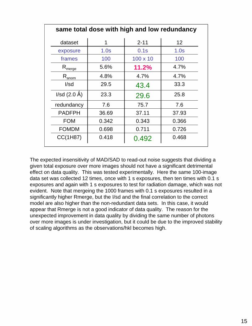
same total dose with high and low redundancy

The expected insensitivity of MAD/SAD to read-out noise suggests that dividing a given total exposure over more images should not have a significant detrimental effect on data quality. This was tested experimentally. Here the same 100-image data set was collected 12 times, once with 1 s exposures, then ten times with 0.1 s exposures and again with 1 s exposures to test for radiation damage, which was not evident. Note that mergeing the 1000 frames with 0.1 s exposures resulted in a significantly higher Rmerge, but the I/sd and the final correlation to the correct model are also higher than the non-redundant data sets. In this case, it would appear that Rmerge is not a good indicator of data quality. The reason for the unexpected improvement in data quality by dividing the same number of photons over more images is under investigation, but it could be due to the improved stability of scaling algorithms as the observations/hkl becomes high.